EXPERIMENT 3a

HEAT TRANSFER IN NATURAL CONVECTION CONTENT:

1. Aim

2. Objective

3. Introduction

4. Theory/Background

5. Apparatus

6. Experimental Procedure

7. Precautions

8. Calculations

9. Uncertainty and Error analysis

10. Result & Discussion

11. References

12. Data Sheet

Note: 1. At least one complete calculation process with equation must be shown in

the beginning of result and discussion part. 2. Students are requested to write their own conclusion in the lab report. 3. Lab report should be submitted within given time.

HEAT TRANSFER IN NATURAL CONVECTION AIM: To determine the natural convection heat transfer coefficient for the vertical cylindrical tube which is exposed to the atmospheric air and losing heat by natural convection.

OBJECTIVE: The purpose of this experiment is to study experimentally the natural convection pipe flows at different heating level.

INTRODUCTION: There are certain situations in which the fluid motion is produced due to change in density resulting from temperature gradients, which is the heat transfer mechanism called as free or natural convection. Natural convection is the principal mode of heat transfer from pipes, refrigerating coils, hot radiators etc. The movement of fluid in free convection is due to the fact that the fluid particles in the immediate vicinity of the hot object become warmer than the surrounding fluid resulting in a local change of density. The warmer fluid would be replaced by the colder fluid creating convection currents. These currents originate when a body force (gravitational, centrifugal, electrostatic etc.) acts on a fluid in which there are density gradients. The force which induces these convection currents is called a buoyancy force which is due to the presence of a density gradient within the fluid and a body force. Grashoff number (Gr) plays a very important role in natural convection.

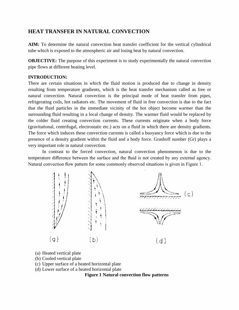
In contrast to the forced convection, natural convection phenomenon is due to the temperature difference between the surface and the fluid is not created by any external agency. Natural convection flow pattern for some commonly observed situations is given in Figure 1.

(a) Heated vertical plate (b) Cooled vertical plate (c) Upper surface of a heated horizontal plate (d) Lower surface of a heated horizontal plate

Figure 1 Natural convection flow patterns

The test section is a vertical, open ended cylindrical pipe dissipating heat from the internal surface. The test section is electrically heated imposing the circumferentially and axially constant wall heat flux. As a result of the heat transfer to air from the internal surface of the pipe, the temperature of the air increases. The resulting density non-uniformity causes the air in the pipe to rise. The present experimental setup is designed and fabricated to study the natural convection phenomenon from a vertical cylinder in terms of the variation of the local heat transfer coefficient and its comparison with the value which is obtained by using an appropriate correlation. THEORY/BACKGROUND: When a hot body is kept in a still atmosphere, heat is transferred to the surrounding fluid by natural convection. The fluid layer in contact with the hot body gets heated, rises up due to the decrease in its density and the cold surrounding fluid rushes in to take its place. The process is continuous and heat transfer takes place due to the relative motion of hot and cold particles. The heat transfer coefficient is given by:

( )s s a

qhA T T

=−

(1)

Here, h = Average surface heat transfer coefficient. q = Heat transfer rate. As = Area of heat transferring surface Ts = Average surface temperature (°C), where,

1 2 3 4 5 6 7

7sT T T T T T TT + + + + + +

= (2)

Ta = Ambient temperature in the duct (°C) = T8

The surface heat transfer coefficient of a system transferring heat by natural convection depends on the shape, dimensions and orientation of the body, the temperature difference between the hot body and the surrounding fluid and fluid properties like κ, µ, ρ etc. The dependence of ‘h’ on all the above mentioned parameters is generally expressed in terms of non-dimensional groups, as follows:

3

2

npChL gL TA

k kµβ

ν ∆

=

(3)

Here,

hLk

is called the Nusselt Number (Nu),

3

2

gL Tβν∆ is called the Grashoff Number (Gr) and,

pCk

µ is called the Prandtl Number

A and n are constants depending on the shape and orientation of the heat transferring surface. L is a characteristic dimension of the surface, κ is the thermal conductivity of the fluid, ν is the kinematic viscosity of the fluid, µ is the dynamic viscosity of the fluid, Cp is the specific heat of the fluid, β is the coefficient of volumetric expansion of the fluid, g is the acceleration due to gravity at the place of experiment, ΔT = Ts -Ta

For gases, 11273f

KT

β −=+

where, Tf = mean film temperature = 2

s aT T+

For a vertical cylinder losing heat by natural convection, the constants A and n of equation (3) have been determined and the following empirical correlations have been obtained:

Nu = thh Lk

= 0.59(Gr.P r)0.25

, for104

< Gr.P r < 109

(4)

Nu = thh Lk

= 0.59(Gr.P r)1/3

, for109

< Gr.P r < 1012

(5)

Here L is the length of cylinder and hth is theoretical heat transfer coefficient. All the properties of the fluid are evaluated at the mean film temperature (Tf ) APPARATUS: The apparatus consists of a stainless steel tube fitted in a rectangular duct in a vertical fashion. The control panel for the natural convection apparatus is shown in figure 2. The heat input to the heater is measured by an ammeter and a voltmeter and is varied by a dimmerstat. The temperatures of the vertical tube are measured by seven thermocouples (1 to 7) and are marked on the Temperature Indicator Switch of the instrument panel as shown in Figure 2. One more thermocouple is used to measure ambient temperature. The schematic of the natural convection apparatus is shown in figure 3.

Figure 2 Control panel for natural convection apparatus

Figure 3. Schematic diagram of natural convection apparatus

The duct is open at the top and the bottom forms an enclosure which serves the purpose of undisturbed surroundings. One side of the duct is made up of perspex for visualization. An electric heating element is kept in the vertical tube which internally heats the tube surface. The heat is lost from the tube to the surrounding air by natural convection. The vertical cylinder with the thermocouple positions is shown in Figure 4.

Figure 4. Thermocouple positions in the vertical cylinder

. While the possible flow pattern and the expected variation of local heat transfer

coefficient are shown in Figure 3. The tube has been polished to minimize the radiation losses.

Figure 5. Variation of the heat transfer coefficient along the height of the tube in free air

flow and dependence of this variation on the nature of flow Specifications:

1. Outer Diameter of the tube (d) = 38 mm 2. Length of the tube (L) = 500 mm 3. Duct size = 20cm × 20cm × 1m length 4. Number of the thermocouples = 8 5. Thermocouple number 8 reads the Ambient Temperature and is kept in the duct.

6. Temperature Indicator 0-300oC. Multi-channel type calibrated from iron constantan

thermocouples with compensation of ambient from 0-50oC.

7. Ammeter 8. Voltmeter 9. Dimmerstat

EXPERIMENTAL PROCEDURE:

1. Switch on the supply and adjust the dimmerstat to obtain the required heat input (say 40 W, 60 W, 70 W).

2. Monitor the temperature T1 to T8 every five minutes till steady state is reached. 3. Wait till the steady state is reached. This is confirmed from temperature readings (T1 to

T7). If they remain steady and do not register a change of more than 1oC per hour.

4. Measure the surface temperature at various points (T1 to T7). 5. Note the ambient temperature, T8. 6. Repeat the experiment for different heat inputs (say 40 W, 60 W, 70 W) by varying

dimmerstat position. PRECAUTIONS:

1. Switch off the ceiling fan before giving supply to set-up. This is to ensure the natural convection heat transfer environment.

2. Adjust the temperature indicator to ambient level by using compensation screw before starting the experiment (if needed).

3. Keep dimmerstat to zero volt position and increase it slowly. 4. Use proper range of Ammeter and Voltmeter. 5. Operate the change over switch of temperature indicator gently from one position to

other, i.e. from position 1 to 8 position. 6. Never exceed 80 W power.

CALCULATIONS:

1. Calculate the value of average surface heat transfer coefficient neglecting radiation losses by experimental method.

Average heat transfer coefficient, ( )avg

s s a

qhA T T

=−

where, q = rate of heating = V I× (watts) As = surface area of vertical cylinder rod = d lπ × × (m2)

Ts = Average surface temperature 1 2 3 4 5 6 7

7T T T T T T T+ + + + + +

= (°C)

Ta = ambient temperature = T8 (°C)

2. Calculate and plot (Figure 4) the variation of the local heat transfer coefficient along the height of the tube using temperature T = T1 to T7 and equation (1).

3. Compare the experimentally obtained values with the theoretically predictions of the cor-relations (4) and (5). All the fluid properties are to be evaluated at mean film temperature.

UNCERTAINTY AND ERROR ANALYSIS: The uncertainty analysis is a long and iterative process that takes the errors in the measured quantities to determine the uncertainty in the computed quantities. For this experiment all the temperatures represent the measured values. The thermocouples had a resolution of 0.1 °C.

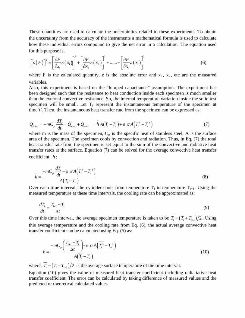
These quantities are used to calculate the uncertainties related to these experiments. To obtain the uncertainty from the accuracy of the instruments a mathematical formula is used to calculate how these individual errors compound to give the net error in a calculation. The equation used for this purpose is,

( ) ( ) ( ) ( )22 2

21 2

1 2

...... ii

F F FF x x xx x x

ε ε ε ε ∂ ∂ ∂

= + + + ∂ ∂ ∂ (6)

where F is the calculated quantity, ε is the absolute error and x1, x2, etc are the measured variables. Also, this experiment is based on the “lumped capacitance” assumption. The experiment has been designed such that the resistance to heat conduction inside each specimen is much smaller than the external convective resistance. So, the internal temperature variation inside the solid test specimen will be small. Let Ti represent the instantaneous temperature of the specimen at time‘t’. Then, the instantaneous heat transfer rate from the specimen can be expressed as:

. . .i

ptotal conv raddTQ mC Q Qdt

= − = + ( ) ( )4 4i a i ah A T T A T Tσ

−

= − +∈ − (7)

where m is the mass of the specimen, Cp is the specific heat of stainless steel, A is the surface area of the specimen. The specimen cools by convection and radiation. Thus, in Eq. (7) the total heat transfer rate from the specimen is set equal to the sum of the convective and radiative heat transfer rates at the surface. Equation (7) can be solved for the average convective heat transfer coefficient, h :

( )

( )

4 4ip i a

i a

dTmC A T Tdth

A T T

σ− −∈ −=

− (8)

Over each time interval, the cylinder cools from temperature Ti to temperature Ti+1. Using the measured temperature at these time intervals, the cooling rate can be approximated as:

1i i idT T Tdt t

+ −=

∆ (9)

Over this time interval, the average specimen temperature is taken to be ( )1 2i i iT T T += + . Using this average temperature and the cooling rate from Eq. (6), the actual average convective heat transfer coefficient can be calculated using Eq. (5) as:

( )

( )

4 41i ip i a

i a

T TmC A T TthA T T

σ+ − − −∈ − ∆ =−

(10)

where, ( )1 2i i iT T T += + is the average surface temperature of the time interval. Equation (10) gives the value of measured heat transfer coefficient including radiatiative heat transfer coefficient. The error can be calculated by taking difference of measured values and the predicted or theoretical calculated values.

RESULTS AND DISCUSSION: Some typical experimental results are shown in Figure 4 for two different heater inputs.

Figure 6. Some typical experimental results

The heat transfer coefficient is having a maximum value at the bottom of the vertical cylinder as expected because of the just starting of the building of the boundary layer and it decreases as expected in the upward direction due to thickening of the boundary layer which is a laminar one. This trend is maintained up to half the height of the cylinder and beyond that there is little variation in the value of the local heat transfer coefficient because of the formation of transition and turbulent boundary layers. The last point shows somewhat increase in the value of ‘h’ which is attributed to end-loss causing a temperature drop.

The comparison of average heat transfer coefficient is also made with predicted values by using correlation (4) and (5). It is found that the predicted values are somewhat less than the experimental values due to heat loss by radiation.

Transfer of energy can occur by three different modes: conduction, convection and radiation. Furthermore, there are two subtypes of convection: forced and natural convection. Forced convection refers to convection in a system with bulk flow while natural convection describes a system where the motion of the fluid arises primarily from naturally occurring density gradients. The rate of heat transfer between a solid surface and the fluid in convection is given by the Newton’s rate equation: qconv = h × A × ((Theater − Ta) (11)

where ‘qconv ’ is the rate of convective heat transfer, ‘A’ is the area normal to direction of heat flow, ’h’ is the convective heat transfer coefficient. Radiation heat transfer is the transfer of heat by electromagnetic radiation. Radiant heat transfer differs from conduction and convection in that no medium is required for its propagation. Energy transfer by radiation is at a maximum when the two surfaces exchanging energy are separated by a vacuum. The basic equation for heat transfer by radiation is:

qrad = A × ε × σ × T 4

(12) where ‘qrad ’ is the rate of radiant heat transfer, ‘A’ is the area of the radiant body, ‘σ’ is

the Stefan-Boltzmann constant which is 5.676×10−8

W/m2K, ‘ε’ is the emissivity, and ‘T’ is the

temperature of the heat absorbing body. When thermal radiation falls upon a body, part is absorbed by the body in the form of

heat, part is reflected back into space, and part may be transmitted through the body. A black body is defined as an object that absorbs all radiant energy and reflects none. The ratio of the emissive power of a surface to that of a black body is called emissivity and for black body, ε =1.0. A radiation heat transfer coefficient, ‘hr ’ is analogous to the convective heat transfer coefficient, is given as: qrad = h1 × A1 × (T1 − T2) (13)

where ‘qrad’ is the rate of heat transfer by radiation,‘A1’ is the surface area of the radiant body, ‘T1’ is the temperature of the radiant body and ‘T2’ is the temperature of the heat absorbing body. To obtain an expression for ‘hr ’ we equate equations, and obtain the following equation:

( )4 4

1 2

1 2r

T Th

T Tε × −

=−

(14)

q = qconv + qrad (15)

The convective heat transfer coefficient is generally between 0-25 W/m2K and for forced

convection 25-500 W/m2K. In calculating the convective heat transfer coefficient, the average

temperature was used, but the air temperature varies in the tube. As a result, the convective heat transfer coefficient calculated is artificially too low. A better approach would be to take the log-mean temperature r to integrate along the length of the tube to find the convective heat transfer coefficient. REFERENCES:

1. Sukhatme, Dr. S.P., A textbook of Heat Transfer, Universities Press 2. Holman, J.P., Heat transfer, McGraw Hill publication 3. Cengel, Y.A., Heat transfer a practical approach, McGraw Hill publication

4. Incropera, F.P., and Dewitt., D. P., Fundamentals of Heat and Mass Transfer, John Wiley & Sons, Inc.

DATA SHEET

OBSERVATIONS:

1. Outer diameter of the cylinder (d) = 38 mm. 2. Length of the cylinder (l) = 500 mm. 3. Voltage = V = (Volts), Current = I = (Amperes) 4. Input to the heater (q) = V × I

Date of Experiment: Name and Roll no. of students: Set#1 V = I = q = Time(min)

Surface Temperature (°C) Ambient Temp (°C)

T1 T2 T3 T4 T5 T6 T7 T8

Set#2 V = I = q =

Time(min)

Surface Temperature (°C) Ambient Temp (°C)

T1 T2 T3 T4 T5 T6 T7 T8

Set#3 V = I = q = Time(min)

Surface Temperature (°C) Ambient Temp (°C)

T1 T2 T3 T4 T5 T6 T7 T8 Summary of results:

Time step

Measured Average Heat Transfer Coeff.

Predicted Average Heat Transfer Coeff.

Difference between measured & predicted h

i h (W/m2K) h (W/m2K) (%)

UNSTEADY STATE HEAT TRANSFER EXPERIMENT 3B

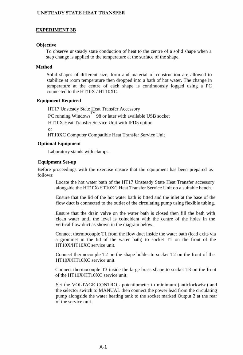
Objective To observe unsteady state conduction of heat to the centre of a solid shape when a step change is applied to the temperature at the surface of the shape.

Method Solid shapes of different size, form and material of construction are allowed to stabilize at room temperature then dropped into a bath of hot water. The change in temperature at the centre of each shape is continuously logged using a PC connected to the HT10X / HT10XC.

Equipment Required

HT17 Unsteady State Heat Transfer Accessory PC running Windows

TM 98 or later with available USB socket

HT10X Heat Transfer Service Unit with IFD5 option or HT10XC Computer Compatible Heat Transfer Service Unit

Optional Equipment Laboratory stands with clamps.

Equipment Set-up Before proceedings with the exercise ensure that the equipment has been prepared as follows:

Locate the hot water bath of the HT17 Unsteady State Heat Transfer accessory alongside the HT10X/HT10XC Heat Transfer Service Unit on a suitable bench.

Ensure that the lid of the hot water bath is fitted and the inlet at the base of the flow duct is connected to the outlet of the circulating pump using flexible tubing.

Ensure that the drain valve on the water bath is closed then fill the bath with clean water until the level is coincident with the centre of the holes in the vertical flow duct as shown in the diagram below.

Connect thermocouple T1 from the flow duct inside the water bath (lead exits via a grommet in the lid of the water bath) to socket T1 on the front of the HT10X/HT10XC service unit.

Connect thermocouple T2 on the shape holder to socket T2 on the front of the HT10X/HT10XC service unit.

Connect thermocouple T3 inside the large brass shape to socket T3 on the front of the HT10X/HT10XC service unit.

Set the VOLTAGE CONTROL potentiometer to minimum (anticlockwise) and the selector switch to MANUAL then connect the power lead from the circulating pump alongside the water heating tank to the socket marked Output 2 at the rear of the service unit. A-1

UNSTEADY STATE HEAT TRANSFER

Note: The voltage control potentiometer is used to set the speed of the circulating pump on this equipment NOT the power to the heating element.

Connect the power lead from the water bath (terminated at the connection box alongside the heating tank) to an electrical supply.

Ensure that the service unit is connected to an electrical supply. Connect the HT10X/HT10XC service unit to the PC using the USB cable provided, and run the HT17 software. Select Exercise A.

Click on the ‘Sample’ menu from the top toolbar, and select ‘Configure…’

In the Sample Configuration menu that appears, check that Sampling Operation is set to Automatic with a Sample Interval of 1 secs and Continuous duration. Change the settings if required. Close the Sample Configuration window by selecting ‘OK’.

Place the various shapes in a suitable location where the metal bodies can stabilize at room temperature. If laboratory stands/clamps are available then the shapes can be suspended from the stands via the insulated rod attached to each shape.

Always pick up the metal shapes via the insulated rod. Heat transferred to the shape by holding in the hand will delay the stabilization of the shape at a uniform temperature.

Note: Since the water bath will take approximately 40 minute to heat to the required temperature it is suggested that this is switched on immediately as described in the Procedure section.

A-2

UNSTEADY STATE HEAT TRANSFER Theory/Background

This exercise is qualitative only and intended to show the transient/time-dependent behaviour of a system where temperature varies with time and position. This condition, referred to as unsteady-state, exists when a solid shape is immersed in the hot water and continues until the whole of the shape reaches equilibrium with the temperature of the water.

When the step change is applied a temperature gradient exists between the surface of the shape at the water temperature and the centre of the shape which is at ambient temperature. Heat flows by conduction through the shape until the whole of the shape is at the same temperature as the water.

Note: The plots of temperature versus time obtained in this exercise can be used in later exercises to perform a quantitative analysis of the unsteady state heat transfer related to the size, form and conductivity of the solid shape.

Procedure

Refer to the Operation section if you need details of the instrumentation and how to operate it. Switch on the front Mains switch (if the panel meters do not illuminate check the RCD and any other circuit breakers at the rear of the service unit, all switches at the rear should be up).

Check that the water heater is filled with water then switch on the electrical supply to the water heater (switch on the RCD which is located on the connection box adjacent to the water heater).

Ensure that the red light is illuminated on the water heater, indicating that electrical power is connected to the unit. Adjust the thermostat on the water heater to setting '4' and check that the red light is illuminated indicating that power is connected to the heating element.

Set the voltage to the circulating pump to 12 Volts, using the control box on the mimic diagram software screen.

Allow the temperature of the water to stabilize (monitor the changing temperature T1 on the software screen). The water must be in the range 80 - 90

oC for satisfactory operation. If outside this

range adjust the thermostat and monitor T1 until the temperature is satisfactory.

Attach the large brass cylinder to the shape holder (insert the insulated rod into the holder and secure using the transverse pin) but do not hold the metal shape or subject it to a change in temperature. Check that the thermocouple attached to the shape is connected to T3 on the HT10X/HT10XC. Check that the thermocouple wire is located in the slot at the top of the shape holder.

Check that the temperature of the shape has stabilized (same as air temperature T2).

Switch off the electrical supply to the water bath (switch off the RCD on the connection box) to minimize fluctuations in temperature if the thermostat switches on/off. A-3

UNSTEADY STATE HEAT TRANSFER

Start continuous data logging by selecting the icon on the software toolbar.

Allow the temperature of the shape to stabilise at the hot water temperature (monitor the changing temperature T3 on the mimic diagram software screen).

When temperature T3 has stabilized, select the icon to end data logging.

Select the icon to create a new results sheet.

Switch on the electrical supply to the water bath to allow the thermostat to maintain the water temperature.

Remove the large brass cylinder from the shape holder then fit the stainless steel cylinder.

Repeat the above procedure to obtain the transient response for the stainless steel cylinder. Remember to create a new results sheet at the end, ready for the next set of results.

Remove the stainless steel cylinder from the shape holder then fit the small brass cylinder. Remember to create a new results sheet at the end, ready for the next set of results.

Repeat the above procedure to obtain the transient response for the small brass cylinder. Remember to create a new results sheet at the end, ready for the next set of results.

If time permits the response of the other shapes can be determined using the same procedure as above.

Results and Calculations The transient behavior of the various shapes is best analysed graphically using graphs of temperature versus time which you have obtained. Graphs can be plotted from the Graph screen of the software. Select the graph screen using the

icon, then select the icon to open the graph configuration screen. The available results are listed on the left. Highlight the first required series (the temperature T3 for the large brass cylinder) and use the red arrow button to transfer it to ‘Series on Primary Axis’, then select ‘OK’. The graph may be printed to a printer (if one is available) by selecting the icon . To print the graph from the next set of results, first highlight the first set and use the red arrow button to transfer it back to ‘Available Series’ before selecting the next set as before.

You should observe the following features on the graphs obtained:

The instantaneous change in temperature T3 corresponds to the instant at which the shape is immersed in the hot water and can be taken as time = 0 seconds for each shape.

Using the large brass cylinder as a reference, the small brass cylinder stabilizes faster because the distance between the centre and the surface of the cylinder is considerably reduced. A-4

UNSTEADY STATE HEAT TRANSFER Because the stainless steel cylinder has a lower conductivity and lower diffusivity than the brass cylinder it takes much longer to stabilize than the brass cylinder of equivalent size. These findings are repeated if the spheres or slabs of different material are compared.

Conclusion

You have observed how, in a solid shape, temperature changes with time and position while heat flows from the hot boundary to heat the cooler material inside of the shape.

This condition of unsteady-state heat transfer exists until the temperature is constant throughout the shape; no temperature gradient exists within the shape when a condition of steady-state is achieved. The time taken for the temperature to stabilise at the centre of the shape depends on the size, form and the material of the solid shape.

A-5

UNSTEADY STATE HEAT TRANSFER

Objective Using analytical transient-temperature/heat flow charts to determine the conductivity of a solid cylinder from the measurements taken on a similar cylinder but having a different conductivity.

Method Cylinders of the same size but different material are allowed to stabilise at room temperature then dropped into a bath of hot water. The change in temperature at the centre of one cylinder is used to determine the heat transfer coefficient for both of the cylinders. This result may then be used to determine the conductivity of the second cylinder.

Note: If results are available from Exercise A then this exercise can be completed using those results. Refer to the Theory section of this exercise followed by the Results and Calculations.

Equipment Required

HT17 Unsteady State Heat Transfer Accessory

PC running WindowsTM

98 or later with available USB socket

HT10X Heat Transfer Service Unit with IFD5 option or HT10XC Computer Compatible Heat Transfer Service Unit

Optional Equipment

Laboratory stands with clamps.

Equipment Setup

Before proceedings with the exercise ensure that the equipment has been prepared as follows:

Locate the hot water bath of the HT17 Unsteady State Heat Transfer accessory alongside the HT10X/HT10XC Heat Transfer Service Unit on a suitable bench.

Ensure that the lid of the hot water bath is fitted and the inlet at the base of the flow duct is connected to the outlet of the circulating pump using flexible tubing.

Ensure that the drain valve on the water bath is closed then fill the bath with clean water until the level is coincident with the centre of the holes in the vertical flow duct as shown in the diagram below. Connect thermocouple T1 from the flow duct inside the water bath (lead exits via a grommet in the lid of the water bath) to socket T1 on the front of the HT10X/HT10XC service unit. B-1

Connect thermocouple T2 on the shape holder to socket T2 on the front of the HT10X/HT10XC service unit.

Connect thermocouple T3 inside the large brass shape to socket T3 on the front of the HT10X/HT10XC service unit.

Set the VOLTAGE CONTROL potentiometer to minimum (anticlockwise) and the selector switch to MANUAL then connect the power lead from the circulating pump alongside the water heating tank to the socket marked Output 2 at the rear of the service unit.

Note: The voltage control potentiometer is used to set the speed of the circulating pump on this equipment NOT the power to the heating element.

Connect the power lead from the water bath (terminated at the connection box alongside the heating tank) to an electrical supply.

Ensure that the service unit is connected to an electrical supply.

Connect the HT10XC service unit to the PC using the USB cable provided, and run the HT17 software. Select Exercise B.

Click on the ‘Sample’ menu from the top toolbar, and select ‘Configure…’

In the Sample Configuration menu that appears, check that Sampling Operation is set to Automatic with a Sample Interval of 1 secs and Continuous duration. Change the settings if required. Close the Sample Configuration window by selecting ‘OK’. B-2

UNSTEADY STATE HEAT TRANSFER

Place the various shapes in a suitable location where the metal bodies can stabilise at room temperature. If laboratory stands/clamps are available then the shapes can be suspended from the stands via the insulated rod attached to each shape.

Always pick up the metal shapes via the insulated rod. Heat transferred to the shape by holding in the hand will delay the stabilisation of the shape at a uniform temperature.

Note: Since the water bath will take approximately 40 minute to heat to the required temperature it is suggested that this is switched on immediately as described in the Procedure.

Theory/Background Analytical solutions are available for temperature distribution and heat flow as a function of time and position for simple solid shapes which are suddenly subjected to convection with a fluid at a constant temperature. A typical chart is included below which is constructed for a long cylinder of radius b where the whole of the surface is suddenly subjected to a change in temperature (the effect of the end faces is considered to be negligible).

To use the charts it is necessary to evaluate appropriate dimensionless parameters as follows:

( ),

i

T r t TT T

θ ∞

∞

−=

−= dimensionless temperature

hbBik

= = Biot number

2

tbατ = = dimensionless time or Fourier number

Where α = Thermal diffusivity of the cylinder (m

2s

-1)

h = Heat transfer coefficient (Wm-2 o

C-1

) k = Thermal conductivity of the cylinder (Wm

-1 oC

-1)

t = Time since step change (seconds) T(0,t) = Temperature at centre of cylinder (=T3 at time t) (

oC)

Ti = Initial temperature of cylinder (T3 at t=0) (oC)

T ∞ = Temperature of water bath (T1) (oC)

b = Radius of cylinder (m) r = Radial position within the cylinder (at axis r = 0) (m) Since the flow of water vertically upwards through the duct is constant for all of the measurements, the heat transfer coefficient h will remain constant for each shape. B-3

Chart for Long Cylinder

B-4

UNSTEADY STATE HEAT TRANSFER

Procedure

Refer to the Operation section in the HT17 instruction manual if you need details of the instrumentation and how to operate it.

Switch on the front Mains switch (if the panel meters do not illuminate check the RCD and any other circuit breakers at the rear of the service unit, all switches at the rear should be up). Check that the water heater is filled with water then switch on the electrical supply to the water heater (switch on the RCD which is located on the connection box adjacent to the water heater).

Ensure that the red light is illuminated on the water heater indicating that electrical power is connected to the unit.

Adjust the thermostat on the water heater to setting '4' and check that the red light is illuminated indicating that power is connected to the heating element.

Set the voltage to the circulating pump to 12 Volts using the voltage control box on the mimic diagram software display.

Allow the temperature of the water to stabilise (monitor the changing temperature T1).

The water must be in the range 80 - 90oC for satisfactory operation. If outside this

range adjust the thermostat and monitor T1 until the temperature is satisfactory.

Attach the large brass shape to the holder (insert the insulated rod into the holder and secure using the transverse pin) but do not hold the metal shape or subject it to a change in temperature. Check that the thermocouple attached to the shape is connected to T3 on the HT10X/HT10XC. Check that the thermocouple wire is located in the slot at the top of the shape holder.

Check that the temperature of the shape has stabilised (same as air temperature T2).

Switch off the electrical supply to the water bath (switch off the RCD on the connection box) to minimise fluctuations in temperature if the thermostat switches on/off).

Start continuous data logging by selecting the icon on the software toolbar.

Allow the temperature of the shape to stabilise at the hot water temperature (monitor the changing temperature T3 on the mimic diagram software screen).

When temperature T3 has stabilised, select the icon to end data logging.

Select the icon to create a new results sheet. Switch on the electrical supply to the water bath to allow the thermostat to maintain the water temperature.

Remove the large brass cylinder from the shape holder then fit the stainless steel cylinder. B-5

UNSTEADY STATE HEAT TRANSFER Repeat the above procedure to obtain the transient response for the stainless steel cylinder.

Remember to create a new results sheet afterwards ready for the next set of results.

Remove the stainless steel cylinder from the shape holder then fit the small brass cylinder.

Repeat the above procedure to obtain the transient response for the small brass cylinder.

If time permits the response of the other shapes can be determined using the same procedure as above. These additional results can be used in exercise HT17C.

Results and Calculations

Determine the value for h using the result obtained for the brass cylinder as follows:

Plot the first graph using the Graph screen of the software. Select the graph screen using

the icon, then select the icon to open the graph configuration screen. The available results are listed on the left. Highlight the first required series (the temperatures T2 and T3 for the large brass cylinder) and use the red arrow button to transfer them to ‘Series on Primary Axis’, then select ‘OK’. The graph may be printed to a printer (if available) by selecting the icon. Establish where t = 0 (i.e. T2 step changes from room temperature to T∞

Choose a point on the temperature/time plot for the brass cylinder and measure the corresponding values of temperature T3 and time t. (the point should be close to the final temperature e.g. 2 or 3 degrees away from the final temperature).

Calculate θ knowing Ti (T3 at t=0), T∞ , and T3 ie. T(r=0, t)

Calculate τ knowing α, t and b (assume α = 3.7 x 10-5

m2s

-1 for brass)

Read value for 1/Bi on chart using the calculated values for θ and τ

Calculate h knowing Bi, b and k (assume k = 121 Wm-1 o

C-1

for brass)

This value of h will be the same for the stainless steel cylinder since the size, shape, surface finish and water velocity are constant.

Plot the graph for the stainless steel cylinder: first highlight the results for the brass cylinder and use the red arrow button to transfer them back to ‘Available Series’. Then select the results for the stainless steel cylinder from the available series, and transfer them to the primary Y-axis. Select ‘OK’, then print the graph (if a printer is available).

Choose a point on the temperature/time plot for the stainless steel cylinder and measure the corresponding values of temperature T at time t. (the point should be close to the final temperature e.g. 2 or 3 degrees away from he final temperature).

Calculate θ knowing Ti (T3 at t=0), T∞ , and T3 i.e. T(r=0, t)

Calculate τ knowing α, t and b (assume α = 0.6 x 10-5

m2s

-1 for stainless steel)

Read value for 1/Bi on chart using the calculated values for θ and τ B-6

UNSTEADY STATE HEAT TRANSFER

Calculate k knowing Bi, b and h (use the calculated value for h obtained using results from the brass cylinder. The typical value of k for stainless steel is 25Wm

-1 oC

-1)

Conclusion

You have experienced the use of analytical transient-temperature/heat flow charts to analyse the temperature changes between the surface and the centre of a solid cylinder.

Relevant dimensionless parameters are used to effect the analysis.

Note: The use of charts, as demonstrated in this exercise, is restricted to simple regular shapes with constant thermal properties. Where bodies have an irregular shape or the surface is not maintained at a uniform temperature then the problems must be solved using a numerical approach such as finite-difference or finite element methods.

B-7