ME 566 Computational Fluid Dynamics for Fluids...

ME 566Computational Fluid Dynamics for

Fluids Engineering DesignANSYS CFX STUDENT USER

MANUAL

Gordon D. StubleyDepartment of Mechanical Engineering, University of

Waterloo

c©G.D. Stubley 2004 - 2006

2007

Contents

1 Getting Started 21.1 Windows XP/NEXUS 21.2 Introduction to Workbench 2

1.2.1 Introduction to DesignModeler/CFX-Mesh GUI 31.2.2 Introduction to the CFX-Post GUI 4

2 The Problem 72.1 The CFD Model Specification 7

3 Geometry and Mesh Specification 103.1 Basic Concepts and Definitions 103.2 Geometry Creation 113.3 CFX-Mesh: Mesh Generation 12

3.3.1 Regions 133.3.2 Mesh Features 13

4 CFX-Pre: Physical Modelling 174.1 Domain 18

4.1.1 Fluids List 184.1.2 Boundary 184.1.3 Domain Models 204.1.4 Fluid Models 20

4.2 Initialization 214.3 Output Control 214.4 Simulation Type 214.5 Solver Control 22

5 CFX Solver Manager: Solver Operation 235.1 Monitoring the Solver Run 23

6 CFX-Post: Visualization and Analysis of Results 266.1 Objects 266.2 Tools 276.3 Controls 28

7 Commands for Duct Bend Example 297.1 Geometry Model 297.2 Mesh Generation 337.3 Pre-processing 357.4 Solver Manager 40

v

vi CONTENTS

7.5 Post-processing 407.6 Clean Up 42

In these notes the basic steps in a CFD solution will be illustrated usingthe professional software ANSYS Workbench Version 10.0 Service Pack 1 whichincludes the components DesignModeler, CFX-Mesh, and CFX (all trademarksof ANSYS). These notes include an introductory tutorial and a mini user’s guide.They are not meant to replace a detailed user’s guide. For full information onthese components refer to the on-line help documentation provided with thesoftware1.

These notes include sections on:Getting Started: Instructions for a short computer session in which the soft-

ware graphical user interfaces, GUIs, are introduced;The Problem: A description of the example problem;The CFD Specification: A complete description of the CFD model imple-

mented in the software;Software Components: A description of the concepts and operation involved

in the five software components: DesignModeler, CFX-Mesh, CFX-Pre, CFX-Solver, and CFX-Post; and

Commands for the Example Problem: A complete step-by-step list of in-structions for solving the model problem.

The following font/format conventions are used to indicate the various com-mands that should be invoked:

Menu/Sub-Menu/Sub-Sub-Menu Item chosen from the menu hierarchy at thetop of a main panel or window,

Button/Tab Command Option activated by clicking on a button or tab,

Link description Click on the description to move by a link to the next step/page;

Name value Enter the value in the named box,

Name H selection Choose the selection(s) from the named list,Name Panel or window name,� Name On/off switch box, and© Name On/off switch circle (radio button).

1Many of the features available in these software components will not be explored in intro-ductory CFD courses.

1

Getting Started

This working session has two purposes:1. to ensure that your Windows XP/NEXUS operating system is operational,

and2. to introduce the look and feel of the software.

1.1 Windows XP/NEXUS

The CFD software is available on the workstations in the Engineering Computinglabs, Fulcrum (E2-1313), Wedge (E2-1302B), Helix (RCH-108), and WEEF (E2-1310), and the Mechanical Engineering 4th year computing room, E2-2354. Theworkstations use the Windows XP operating system on Waterloo NEXUS. Youshould be familiar with techniques to create new folders (or directories), to deletefiles, to move through the folder (directory) system with Windows Explorer, toopen programs through the Start menu on the Desktop toolbar, to move, resize,and close windows, and to manage disk space usage with tools like WinZip.

1.2 Introduction to Workbench

The ANSYS Workbench environment provides an interface to manage the filesand databases associated with the individual software components. These filesand databases are organized into a particular project. To get a feel for thisenvironment and the GUIs associated with the software components, we willlook at a pre-prepared project on flow through a pipe bend.

1. Create a working directory called CFDTest on your N drive.2. Use a web browser to visit the UW-ACE ME 566 course page (uwace.uwaterloo.ca).

Under the Lessons tab and open the Student User Manual folder. Click onthe link to PipeBend.zip and follow the instructions to download the archivecontaining the working files.

3. Use WinZip to extract the files in the PipeBend archive into your workingdirectory.

4. Open ANSYS Workbench fromStart/Programs/Engineering/ANSYS 10.0/ANSYS Workbench.

5. Open the project file. Check that Open: H Workbench Project is selected

before using the Browse button below the Open: Workbench Projects

2

INTRODUCTION TO WORKBENCH 3

panel area to find and selecting the file PipeBend.wbdb from your workingdirectory.

6. There are three main areas on the screen: command menus, buttons, andtabs at the top, a list of potential Project Tasks on the left, and a list of thefiles linked to the project.

7. On-line help for Workbench, DesignModeler, and CFX-Mesh is available inweb-page format similar to other Windows programs. Choose Help/ANSYSWorkbench Help to open the ANSYS Workbench Documentation. Searchfor keyword Tutorials and select CFX-Mesh Help. Follow the Tutorials linkto see the list of available tutorials.

1.2.1 Introduction to DesignModeler/CFX-Mesh GUI

1. In the Workbench file area click on the item name PipeBend just to theright of the DesignModeler button ( DM ). Notice that the Project Tasksarea at the left adjusts to reflect your choice. Under DesignModeler Taskschoose Open to open the geometry file.

2. A new page for DesignModeler will open. Go back to the Project page byclicking on the PipeBend [Project] tab at the top left of the screen. Click

on the PipeBend [DesignModeler] tab to return to the DesignModelerpage.

3. There are four major areas on the page: command menus and buttons atthe top, a Tree View and Sketch Toolbox on the left, a Details View at thebottom left, and a Model View window. Place the mouse cursor over oneof the command buttons in the top row. A brief description of the button’saction should appear (you may need to click in the window once to make itactive). Visit each button with the mouse cursor to see its action.

4. One method of controlling the view is with the coordinate system triad inthe lower right corner of Model View. Click on the Z axis of the triad tosee a back view of the pipe bend. Click on the cyan sphere to select theisometric view.

5. Another method of controlling the view is with the mouse left button inconjunction with a mouse action selection. From the upper row of buttons,select the Pan action. Holding the left mouse button down, drag the mouseover the Model View to translate the view. Select the Zoom action andrepeat the mouse action to change the size of the view.

6. Select the Rotate action. The rotate action is context sensitive in thatit depends upon the position of the mouse cursor. With the mouse cursorclose to the pipe bend, press the left mouse button to get free 3D rotation.The point of rotation can be changed by clicking the left button while thecursor is on the pipe bend surface (this may take some experimentation).With the mouse cursor in a corner of the Model View, press and hold theleft mouse button to get a roll action in which there is 2D rotation aboutan axis perpendicular to the Model View window. Move the cursor to either

4 GETTING STARTED

the left or right of the Model View and hold the left button to get a yawaction in which there is 2D rotation about the vertical axis. Move the cursorto either the top or bottom of the Model View and hold the left button toget a pitch action in which there is 2D rotation about the horizontal axis.

7. Rotate, zoom, and pan actions can be achieved directly by pressing themiddle mouse key alone, with the Shift key, and with the Ctrl key, respec-tively.

8. The Tree View on the left shows the geometric entities that were used togenerate the cylinder. Expand the 1 Part, 1 Body entity and click on Solidto see some properties of the cylinder in the Details View. The pipe bendwas generated from two entities:(a) Sketch1: which can be found in the Plane4 entity. Click on Sketch1 to

highlight the circle that the pipe bend is based upon with yellow.(b) Sketch2:. which can be found in the YZPlane entity. Click on the

Sketch2 to highlight the path that is swept out by Sketch1 to gener-ate the pipe bend.

9. In the help page search for keywords rotation modes and select CFX-MeshHelp to find more information on changing the view.

10. Click the X button on the PipeBend [DesignModeler] tab to close theDesignModeler page. You can click No to quit without saving changes.

1.2.2 Introduction to the CFX-Post GUI

The tasks associated with CFD simulation in Workbench are referred to as Ad-vanced CFD Tasks. For historical reasons, there are differences in the GUI andHelp files for the three CFX components. We will use CFX-Post to look at thecompleted simulation of flow through a pipe bend to get a feel for these interfaces.

1. In the Workbench file area click on the item name PipeBend 001. UnderAdvanced CFD Tasks, choose Open in CFX-Post to open the results file(PipeBend 001.res). All of the pertinent CFD model data (mesh, flow at-tributes, and boundary condition information) for this problem is stored inthis file.

2. A new page for CFX-Post will open.3. There are three major areas on the screen: Command menus and buttons at

the top, selector and edit panels on the left, and Viewer window. Wireframemodels of the pipe inlet and outlet should be in the Viewer. To see the pipebend click the � Domain 1 Default object on in the Objects panel.

4. The mouse button action for controlling the view is similar to that in De-signModeler. There is a significant difference in that the rotation action isnot context sensitive. 2D rotation about an axis perpindicular to the screenis achieved by pressing the Ctrl key with the left button while in rotationmode.

5. The coordinate system triad is shown in the lower right corner. Unlike inDesignModeler, the triad cannot be used to change the view. The view can

INTRODUCTION TO WORKBENCH 5

be changed with the view buttons at the top of the Viewer window. Use the-X to select an orthographic view towards -x along the x axis.

6. Now look at some results. Each visualization is created by defining a newvisualization object and then editing the properties of the object. To makea vector plot along the centre plane of the pipe bend:(a) Choose Create/Location/Plane from the top menu row (or click on

the Location H Plane rolldown menu. In the New Plane panel acceptName Plane 1 , and click Ok to open a Plane edit panel in the lowerleft. In the edit panel set:• Domains H All Domains (the default),• Method H YZ Plane , X 0 , � Visibility on

and click Apply . To see this plane, click the � Domain 1 Default

object off in the Objects panel.(b) Choose Create/Vector from the top menu row (or use the corresponding

button on the second row). In the New Vector panel accept Name

Vector 1 , and click OK to open a Vector edit panel. In the editpanel set:• Locations H Plane 1 ,• Variable H Velocity ,• © Hybrid on,• Projection H None ,• Reduction Reduction Factor ,• Factor 10 ,• � Visibility on

and click Apply . The vector plot should appear in the Viewer windowand the vector object should be listed in the Object database panel.Open the the View Control branch in the Object tree and turn �DEFAULT LEGEND off and back on to remove and then replace thescale legend.

7. To visualize the pressure field, create a contour plot. Remove the vectorplot, click � Vector 1 and � Plane 1 off in the Object tree. Choose Cre-ate/Contour from the top menu row. In the New Contour panel acceptName Contour 1 , and click OK . In the Contour - Contour 1 edit panelset:• Locations H Plane 1 ,

• Variable H Pressure ,• © Hybrid on,• Colour Scale H Linear ,

• Colour Map H Rainbow ,• # of Contours 10 ,• � Visibility on

6 GETTING STARTED

and click Apply . The fringe plot should appear in the Viewer window. Go

to the Render tab in the Contour edit panel , turn � Draw Faces off,and click Apply to see a line contour plot of the pressure field. Does thispressure field make sense to you?

8. On-line help is available in Java html file format, Help. Open the main tableof contents, Help/Master Contents. Context-sensitive help is also available.Position the mouse pointer in the Object Selector panel and press <F1> tobring up the help page for that panel.

9. This should give a sense of the operation of the CFX GUI. Feel free toexperiment with other object types and scalar fields. When you have fin-ished, return to the Workbench Project page. Exit by File/Close Projectand choose No: do not save any items.

10. Clean up by deleting the CFXTest directory.

2

The Problem

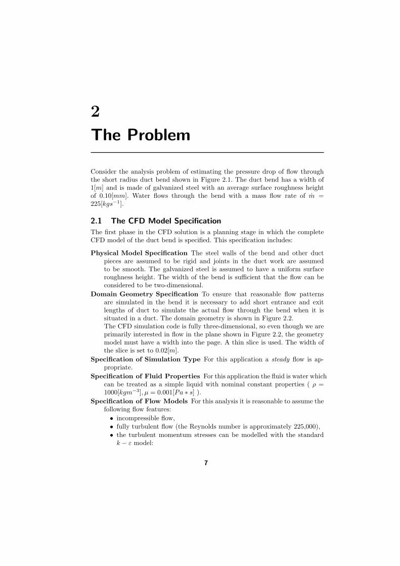
Consider the analysis problem of estimating the pressure drop of flow throughthe short radius duct bend shown in Figure 2.1. The duct bend has a width of1[m] and is made of galvanized steel with an average surface roughness heightof 0.10[mm]. Water flows through the bend with a mass flow rate of m =225[kgs−1].

2.1 The CFD Model Specification

The first phase in the CFD solution is a planning stage in which the completeCFD model of the duct bend is specified. This specification includes:

Physical Model Specification The steel walls of the bend and other ductpieces are assumed to be rigid and joints in the duct work are assumedto be smooth. The galvanized steel is assumed to have a uniform surfaceroughness height. The width of the bend is sufficient that the flow can beconsidered to be two-dimensional.

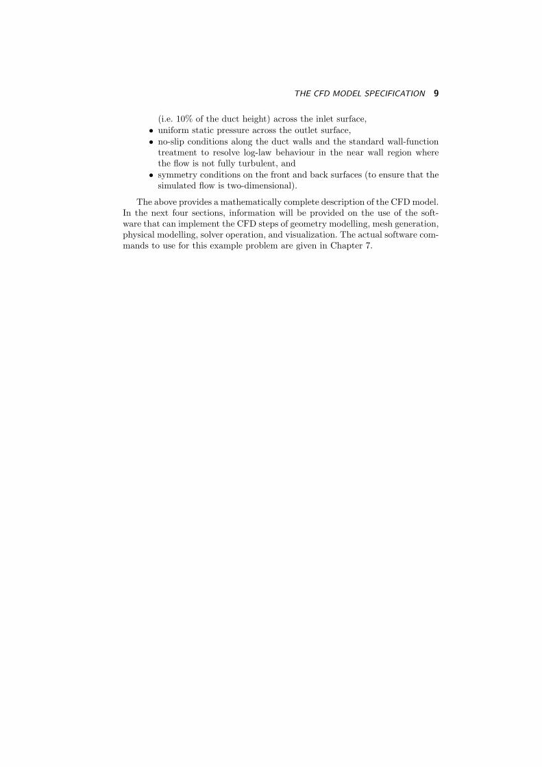
Domain Geometry Specification To ensure that reasonable flow patternsare simulated in the bend it is necessary to add short entrance and exitlengths of duct to simulate the actual flow through the bend when it issituated in a duct. The domain geometry is shown in Figure 2.2.The CFD simulation code is fully three-dimensional, so even though we areprimarily interested in flow in the plane shown in Figure 2.2, the geometrymodel must have a width into the page. A thin slice is used. The width ofthe slice is set to 0.02[m].

Specification of Simulation Type For this application a steady flow is ap-propriate.

Specification of Fluid Properties For this application the fluid is water whichcan be treated as a simple liquid with nominal constant properties ( ρ =1000[kgm−3], µ = 0.001[Pa ∗ s] ).

Specification of Flow Models For this analysis it is reasonable to assume thefollowing flow features:• incompressible flow,• fully turbulent flow (the Reynolds number is approximately 225,000),• the turbulent momentum stresses can be modelled with the standard

k − ε model:

7

8 THE PROBLEM

��PP� ��NJ�V�

��P

��P

Fig. 2.1 Geometry of short radius duct bend

��P

��P

Fig. 2.2 Geometry of the duct bend model

τij = µt

(∂Uj

∂xi+

∂Ui

∂xj

)(1)

where the turbulent viscosity, µt, is proportional to the fluid density,the velocity scale of the turbulent eddies and the length scale of theeddies. The scales of the turbulent eddying motion are estimated fromtwo field variables which are calculated as part of the model: k, theturbulent kinetic energy, and ε, the rate at which k is dissipated bymolecular viscous action.

Specification of the Boundary Conditions The boundary conditions thatmodel the interaction of the surroundings with the solution domain are:• uniform velocity of 3[ms−1] and uniform turbulence properties of tur-

bulence intensity of 5% and turbulence eddy length scales of 0.0075[m]

THE CFD MODEL SPECIFICATION 9

(i.e. 10% of the duct height) across the inlet surface,• uniform static pressure across the outlet surface,• no-slip conditions along the duct walls and the standard wall-function

treatment to resolve log-law behaviour in the near wall region wherethe flow is not fully turbulent, and

• symmetry conditions on the front and back surfaces (to ensure that thesimulated flow is two-dimensional).

The above provides a mathematically complete description of the CFD model.In the next four sections, information will be provided on the use of the soft-ware that can implement the CFD steps of geometry modelling, mesh generation,physical modelling, solver operation, and visualization. The actual software com-mands to use for this example problem are given in Chapter 7.

3

Geometry and MeshSpecification

In the first steps of the CFD computer modelling, the solution domain is cre-ated in a digital form and then subdivided into a large number of small finiteelements or volumes. Common finite element types (shapes) include: tetrahedral,prismatic, and hexahedral. These notes present a basic methodology for develop-ing simple geometries for tetrahedral meshes.

3.1 Basic Concepts and Definitions

Vertex: Occupies a point in space. Often other geometric entities like edgesconnect at vertices.

Edge: A curve in space. An open edge has beginning and end vertices at distinctpoints in space. A straight line segment is an open edge. A closed edge hasbeginning and end vertices at the same point is space. A circle is a closededge.

Face: An enclosed surface. The surface area inside a circle is a planar face andthe outer shell of a sphere is a non-planar face. An open face has all ofits edges at different locations in space. A rectangle makes an open face.A closed face has two edges at the same location in space. The cylindricalsurface of a pipe is a closed face.

Solid: The basic unit of three dimensional geometry modelling:• is a space completely enclosed in three dimensions by a set of faces

(volume);• the surface faces of the solid are the the external surface of the flow

domain; and• holes in the solid represent physical solid bodies in the flow domain such

as airfoils.Part: One or more solids that form a flow domain.Multiple Solids: May be used in each part:

• the solid volumes cannot overlap;• the solids must join at common surfaces or faces; and• the faces where two solids join can be thin surfaces

10

GEOMETRY CREATION 11

Thin Surface: A thin solid body in a flow like a guide vane or baffle can bemodelled as an infinitely thin surface with no-slip walls on both sides.

Units: To keep things simple and to minimize errors, use metric units through-out.

Advanced Concepts: See the Geometry section of the CFX-Mesh Help for fur-ther information on geometry modelling requirements. To develop improvedskill follow the tutorials given in CFX-Mesh Help/Tutorials.

3.2 Geometry Creation

The basic procedure for creating a three dimensional solid geometry is to make a2D sketch of an enclosed area (possibly with holes) on a flat plane. The resulting2D sketch is a profile which is swept through space to create a 3D solid feature.This process can be repeated to either remove portions of the 3D solid or to addportions to the solid.

Each sketch is made on a Plane:• There are three default planes, XYPlane, XZPlane, and YZPlane, which

coincide with the three planes of the Cartesian coordinate system;• Each plane has a local X-Y coordinate system and normal vector (the plane’s

local Z axis);• New planes can be defined based on: existing planes, faces, point and edge,

point and normal direction, three points: origin, local X axis, and anotherpoint in plane, and coordinates of the origin and normal; and

• Plane transforms such as translations and rotations can be used to modifythe base definition of the plane.

The creation of a sketch is similar to the creation of a drawing with moderncomputer drawing software:• A sketch is a set of edges on a plane. A plane can contain more than one

sketch;• The sketching toolbox contains tools for drawing a variety of common two

dimensional shapes;• Dimensions are used to set the lengths and angles of edges;• Constraints are used to control how points and shapes are related in a

sketch. Common constraints include:Coincident (C): The selected point (or end of edge) is coincident with

another shape. For example, the end point of a new line segment can beconstrained to lie on the line extending from an existing line segment.Note that the two line segments need not touch;

Coincident Point (P): The selected points are coincident in space;Vertical (V): The line is parallel to the local plane’s Y axis;Horizontal (H): The line is parallel to the local plane’s X axis;Tangent (T): The line or arc is locally tangent to the existing line or arc;Perpendicular (⊥): The line is perpendicular to the existing line; andParallel (‖): The line is parallel to the existing line.

12 GEOMETRY AND MESH SPECIFICATION

As a sketch is drawn the symbols for each relevant constraint will appear. Ifthe mouse button is clicked while a constraint symbol is on the sketch thenthe constraint will be applied. Note that near the X and Y axes it is oftendifficult to distinguish between coincident and coincident point constraints;and

• Auto-Constraints are used to automatically connect points and edges. Forexample, if one edge of a square is increased in length the opposite edgelength is also increased so that the shape remains rectangular.

Features are created from sketches by one of the following operations:

Extrude: Sweep the sketch in a particular direction (i.e. to make a bar);Revolve: Sweep the sketch through a revolution about a particular axis of ro-

tation (i.e. to make a wedge shape);Sweep: Sweep the sketch along a sketched path (i.e. to make a curved bar); andSkin/Loft: Join up a series of sketches or profiles to form the 3D feature (like

putting a skin over the frame of a wing).

Features are integrated into the existing active solid with one of the followingBoolean operations:

Add Material: Merge the new feature with the active solid;Cut Material: Remove the material of the new feature from the active solid;Slice Material: Remove a section from an active solid; andImprint Face: Break a face into two parts. For example, this will open a hole

on a cylindrical pipe wall.

Sometimes it is necessary to use multiple solids in a single part. These solidsmust share at least one common face. This common face might be used to modela thin surface in the flow solver. In this case:

1. Select active solid with the body selection filter turned on;2. Freeze the solid body to stop the Boolean merge or remove operations

(Tools/Freeze). This will form a new solid body as a component of a newpart; and

3. Select all solids and choose Tools/Form New Part.

When the solid model is completed an .agdb file is created and saved in orderto store the geometry database.

3.3 CFX-Mesh: Mesh Generation

The mesh generation phase can be broken down into the following steps:

1. Read in or update the .agdb file with the solid body geometry database;2. Set the properties of the mesh;3. Cover the surfaces of the solid body with a surface mesh of triangular or

quadrilateral elements; and4. Fill the interior of the solid body with a volume mesh of tetrahedral, hex-

ahedral, or prism elements that are based on the surface meshes and that

CFX-MESH: MESH GENERATION 13

�� !��"�

#$��%�&�'��(��)�*��%�+�,��(�%�-�.�� /�+�"�

�0�1��2,��34��-�1��%�� 5��"� ��%��,�4� �%�4��6��%�" ��%�� 5��"�

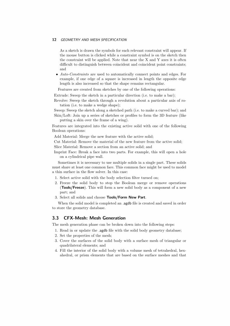
Fig. 3.1 Shapes of common two and three dimensional elements.

grow inwards from each surface mesh. A .gtm file containing all of the meshinformation and region information is written at the end of this step.

The following comments and guidelines are for generating tetrahedral mesheswith surface inflation for two-dimensional flow simulation in relatively simplerectangular geometries.

3.3.1 Regions

The geometry database contains a list of primitive faces and edges that areformed in the generation processes. It is often cumbersome to work directly withthese primitive entities. Therefore, there is a facility for creating and namingcomposite 2D surface regions. When the mesher is initialized all of the primitive2D surfaces are assigned to the Default 2D Region. As surfaces are assigned tonew user defined regions they are removed from the Default 2D Region. However,the Default 2D Region must contain at least one surface. These region namesand their corresponding surface meshes are passed on to CFX-Pre.

3.3.2 Mesh Features

The mesh is composed of two dimensional triangular elements on the surfacesand tetrahedral and prism elements in the body of the solid. Figure 3.1 showsthe element shapes.

The properties of the mesh are controlled by the settings of the followingfeatures:

Default Body Spacing: Set the maximum length scale of the tetrahedral ele-ments throughout the volume of the body. Some of the actual tetrahedralelements may be smaller due to the action of other mesh features or in orderto fit the tetrahedral elements into the body shape.

Default Face Spacing: Set the length scale of the triangular elements on thesurfaces.


• For simple meshes it is sufficient to set Face Spacing Type H Volume Spacing .• For surfaces such as an airfoil in a large flow domain, it might be desir-

able to set the triangular mesh length scale smaller than the defaultbody spacing. In this case a new Face Spacing can be defined andassigned to the airfoil surface. Besides setting the triangular elementlength scale, the following properties must be set for the new face spac-ing:Radius of Influence: The distance from the region that has a tetra-

hedral mesh length scale equal to that of the surface triangularelements;

Expansion Factor: The rate at which the tetrahedral mesh length scaleincreases outside the radius of influence. This value controls howsmoothly the mesh length scale increases from the face region tothe default body spacing far from from the face.

• For complex surfaces the face spacing type should set so that the ge-ometry of the surface is well represented by the mesh: relative error orangular resolution.

Controls: are used to locally decrease the mesh length scale in the region arounda point, line, or triangular plane surface. The spacing in the vicinity of acontrol is set by three factors:Length Scale: fixes the size of the tetrahedral mesh elements;Radius of Influence: sets the distance from the control that has a mesh of

the specified length scale; andExpansion Factor: controls how smoothly the mesh length scale increases

to the default body spacing far from the control.For line and triangle controls, the spacing can be varied over the control(i.e. from one end point of the line to the other end point).

Extruded Periodic Pair: In cases where the flow is two dimensional, it is desir-able to have a single mesh element in the cross-stream direction. In thesecases the surface meshes on two surfaces will need to be identical (i.e. the facemesh on the first surface can be uniquely mapped onto the second surface).In other cases where the flow is three dimensional, it may still be desirableto have identical face meshes on two bounding surfaces. For example, thisis useful in periodically repeating geometries.Each Periodic Pair is defined by two surfaces and a two dimensional pla-nar (Periodic Type H Translational ) or axisymmetric (Periodic Type H

Rotational ) mapping.Inflation: In boundary layer regions adjacent to solid walls it is often desirable

to make a very small mesh size in the direction normal to the wall in orderto resolve the large velocity shear strain rates. If tetrahedral meshes are usedin this region there will either be a large number of very small elements withequal spacing in all directions (i.e. isotropic elements with vertex angles closeto 60◦) or very thin squashed elements. These choices are either inefficientor inaccurate. A better element shape in this region is a triangular prism,

CFX-MESH: MESH GENERATION 15

Figure 3.1, based on the surface triangular mesh. The basic shape of theprism element is independent of the height of the prism (mesh length scalenormal to the wall). The layer of prism elements is an inflated boundarywith:Maximum Thickness: that is often approximately the same as the default

body mesh spacing; orFirst Layer Thickness: that is often set by the properties of the local tur-

bulent boundary layer. Other properties include:Number of Inflated Layers: specifies the number of prism elements across

the thickness of the inflated layer; andExpansion Factor: specifies how the prism height increases with each in-

flated layer above the wall surface. This factor must be between 1.05and 1.35.

Stretch: The default body mesh length scale is isotropic. The vertex angles inthe isotropic tetrahedral elements are close to 60◦. In geometries that arenot roughly square in extent, it may be desirable make the mesh length scalelonger or shorter in one particular direction. This is achieved by stretchingthe geometry in a given direction, meshing the modified geometry with anisotropic mesh, and then returning the geometry (along with the mesh) toits original size. This means that if the y direction is stretched by a factor of0.25 without stretching in the other two directions then the mesh size in they direction will be roughly 4 times that of the other directions. Take care toensure that the resulting tetrahedral elements do not get too squashed. Forthis reason the stretch factors should be between 0.2 and 5 at the very most(more moderate stretch factors are desirable). Note: stretch parameters areignored in extruded meshes.

Proximity: flags set the behaviour of the mesh spacing when edges and sur-faces become close together. For simple rectangular geometries set Edge

Proximity H No and Surface Proximity H No .Options: are used for setting the output filename and for setting the algorithms

used for generating the volume and surface meshes:

Surface Meshing H Delaunay is a fast algorithm for creating isotropicsurface meshes. Suited to complex surface geometries with small meshspacing.

Surface Meshing H Advancing Front starts at the edges of the surface andis a similar algorithm to the volume meshing algorithm described above.Since it creates regular meshes on simple rectangular type surfaces, itis the recommended algorithm.

Meshing Strategy H Extruded 2D Mesh is an algorithm for generatingmeshes in geometries that are effectively 2D. A surface mesh is ex-truded through space by either translation or rotation from one face toa matching face in the periodic pair. This option is useful for simulatingtwo dimensional flows and flows in long constant area ducts. The num-


ber of elements (often 1) and mesh spacing distribution in the extrudeddirection can be specified.

Meshing Strategy H Advancing Front and Inflation 3D is the primary al-gorithm for generating meshes in 3D geometries. The algorithm startswith a surface mesh and then builds a layer of tetrahedral elements overthe surface based on the surface triangular elements. This creates a newsurface. The process is repeated advancing the layers of tetrahedral el-ements into the interior of the volume.

Volume Meshing H Advancing Front does the calculations with a singlecomputer. An option for generating the volume mesh in parallel on anetwork of computers exists.

4

CFX-Pre: Physical Modelling

CFX-Pre is a program that builds up a database for storing all of the informa-tion (geometry, mesh, physics, and numerical methods) that is required by theequation solver. The contents of the database is written to a def (definition) fileat the end of the CFX-Pre session.

The database is organized as a hierarchy of objects. Each object in the hier-archy is composed of sub-objects and parameters. There are two main objects:Flow and Library. The Flow object holds all of the data on the flow modeland the Library object holds the property data for the fluids.

The major components of the Flow object are organized in the followinghierarchy:

• Flow

∗ Domain◦ Fluids List (not explicitly shown in the Physics panel)◦ Boundary◦ Domain Models

– Domain Motion– Reference Pressure

◦ Fluid Models– Heat Transfer Model– Turbulence Model– Turbulent Wall Functions

∗ Initialization∗ Output Control∗ Simulation Type∗ Solver Control

◦ Advection Scheme◦ Convergence Control◦ Convergence Criteria

CFX-Pre has functions to create new objects in the hierarchy and to editexisting objects through edit panels. For most objects, the edit panel providesguidance on the possible parameter settings.

17

18 CFX-PRE: PHYSICAL MODELLING

4.1 Domain

4.1.1 Fluids List

A fluid (or mixture of fluids in more complex multi-phase flows) has to be asso-ciated with each domain. The fluid for a particular domain can be selected fromthe fluid library which has many common fluids. The Materials panel managesthe fluid library. There are provisions for selecting pre-defined fluids, definingnew fluids, and creating duplicates or copies of existing fluids.

The properties of fluids can be general functions of temperature and pressurefor liquids or gases. The CFX Expression Language, CEL is used to input for-mulae for specifying equations of state and other applications such as boundaryvariable profiles, initialization, and post-processing. CEL allows expressions withstandard arithmetic operators, mathematical functions, standard CFX variables,and user-defined variables. All values must have consistent units and variablesin CEL expressions must result in consistent units. Full details of CEL, includ-ing the names of the standard CFX variables, are included in the ANSYS CFXReference Guide.

For low speed flows of gases and liquids it is adequate to use constant propertyfluids. It is easiest to build up a new constant property fluid from a comparablefluid from the existing CFX fluid library as a template. For example, to defineconstant property air at 20 ◦C, make a duplicate copy of air at 25 ◦C and thenedit this copy.

4.1.2 Boundary

Throughout each domain, mass and momentum conservation balances are ap-plied over each element. These are universal relationships which will not distin-guish one flow field from another. To a large extent, a particular flow field for aparticular geometry is established by the boundary conditions on the surfaces ofthe domain.

A standard boundary condition object includes a name, a type, a set ofsurfaces, and a set of parameter values. In CFX-Post the boundary conditionobject name is used to refer to the set of surfaces on which the boundary conditionis applied. For this reason the habit of naming each boundary condition by thename of its surfaces (as defined in CFX-Mesh) is often followed.

Boundary condition types include:Inlet: an inlet region is a surface over which mass enters the flow domain. For

each element face on an inlet region, one of the following must be specified:• fluid speed and direction (either normal to the inflow face or in a par-

ticular direction in Cartesian coordinates),• mass flow rate and flow direction, or• the total pressure -

Ptotal ≡ P +12ρV 2 = Ptotalspec (1)

and flow direction

DOMAIN 19

If the flow is turbulent then it is necessary to specify two properties of theturbulence. Most commonly, the intensity of the turbulence -

I ≡ Average of speed fluctuations

Mean speed(2)

and one additional property of the turbulence: the length scale of the turbu-lence (a representative average size of the turbulent eddies), or eddy viscos-ity ratio (turbulent to molecular viscosity ratio, µt/µ) are specified. Typicalturbulence length scales are 5% to 10% of the width of the domain throughwhich the mass flow occurs.

Outlet: an outlet region is a surface over which mass leaves the flow domain.For each element face on an outlet region, one of the following must bespecified:• fluid velocity (speed and direction),• mass flow rate, or• static pressure

A specified static pressure value can be set to a specific face, applied as aconstant over the outflow region, or treated as the average over the outflowregion. No information is required to model the turbulence in the fluid flowat an outflow.

Opening: a region where fluid can enter or leave the flow domain. Pressure andflow direction must be specified for an opening region. If the opening regionwill have fluid entering/leaving close to normal to the faces (i.e. a windowopening) then the specified pressure value is the total pressure on inflowfaces and the static pressure on outflow faces (a mixed type of pressure). Ifthe opening region will have fluid flow nearly tangent to the faces (i.e. thefar field flow over an airfoil surface) then the specified pressure is a constantstatic pressure over the faces. For turbulent flows, the turbulence intensitymust also be set.

Wall: a solid wall through which no mass can flow. The wall can be stationary,translating (sliding), or rotating. If the flow field is turbulent then the wallcan be either smooth or rough. Depending upon which of these optionsare chosen, suitable values must be input (i.e. the size of the roughnesselements).

Symmetry: a region with no mass flow through the faces and with negligibleshear stresses (and negligible heat fluxes). This condition is often used tosimulate a two-dimensional flow field with a three-dimensional flow solverand to minimize mesh size requirements by taking advantage of naturalsymmetry planes in the flow domain.

Since it is crucial that each surface element face have a boundary conditionattached to it, CFX-Pre automatically provides a default boundary condition foreach domain. Once all boundary surfaces have been attached to explicit boundaryconditions, the default boundary condition object is deleted. This allows the userto identify surfaces which still require explict boundary conditions.


Inlet Sets Outlet Sets Solution Predictsvelocity static pressure inflow static pressuretotal pressure velocity outflow pressure

inflow velocitytotal pressure static pressure system mass flow

Table 4.1 Common boundary condition combinations

For the flow solver to successfully provide a simulated flow field, the spec-ified boundary conditions should be realizable (i.e. they should correspond toconditions in a laboratory setup). In particular, ensure that the inlet and outletboundary conditions are consistent and that they take advantage of the knowninformation. Table (4.1) lists several common inlet/outlet condition combinationsalong with the global flow quantity which is estimated as part of the solution foreach combination.

4.1.3 Domain Models

In incompressible flow fields, the actual pressure level does not play any rolein establishing the flow field - it is pressure differences which are important.The solver calculates these pressure differences with respect to a reference pres-sure. Solution fields are in relative pressure terms but absolute pressure (relativepressure plus reference pressure) is used for equation of state calculations.

In turbomachinery applications it is convenient to analyse the flow in a ro-tating reference frame. In this case, the domain is in a rotating reference frameand its axis of rotation and rotation rate must be specified.

4.1.4 Fluid Models

Heat Transfer Model: options include:None: no temperature field is computed (not an applicable option for ideal

gases),Isothermal: a constant temperature field is used,Thermal Energy: a low speed (neglecting kinetic energy effects) form of

the enthalpy conservation equation is computed to provide a tempera-ture field, and

Total Energy: a high speed form for conservation of energy including ki-netic energy effects is computed.

Turbulence Model: options include:None: laminar flow simulation,k-Epsilon: the accepted state-of-the-art turbulence model involves the so-

lution of two transport equations,Shear Stress Transport: a variant of the k-Epsilon model that provides

a higher resolution solution in near wall regions, andBSL and SSG Reynolds Stress: two variants of second moment closure

models that explicitly solve transport equations for all six components

INITIALIZATION 21

of the turbulent stress tensor and that require significantly more com-puting resources than the two equation variations.

Turbulent Wall Functions: are required to treat the transition to laminarlike flow close to solid walls. The wall treatments are tied to the turbulencemodel choice. The scalable wall function method used with the k-Epsilonturbulence model is a variant of the standard wall function method. Thescalable wall function method automatically adjusts the near wall treatmentwith mesh spacing in the near wall region.

4.2 Initialization

The algebraic equation set that must be solved to find the velocity and pressureat each mesh point is composed of nonlinear equations. All strategies for solvingnonlinear equation sets involve iteration which requiring an initial guess for allsolution variables. For a turbulent flow, sufficient information must be providedso that the following field values can be set (initialized) at each mesh point:

• velocity vector (3 components),• fluid pressure,• turbulent kinetic energy, and• dissipation rate of turbulent kinetic energy.

CFX-Pre provides a default algorithm for calculating initial values based oninterpolating boundary condition information into the interior of the domain.This default algorithm is adequate for many simulations.

The initial conditions can significantly impact the efficiency of the iterativesolution algorithm. If there are condition difficulties then values or expressions(with CEL) can be used to provide intial conditions that:

• match the initial conditions to the dominant inlet boundary conditions, and• align the flow roughly with the major flow paths from inlet regions to outlet

regions.

4.3 Output Control

For many simulation cases, especially those with a strong emphasis on fluid me-chanics, it is necessary to output additional fields to the res output data file.For example, it is often worthwhile to output the turbulent stress fields through-out the flow domain, wall shear stresses on all boundary walls, and gradientoperations applied to all primary solution variables.

4.4 Simulation Type

The numerical formulations for steady and transient flows differ slightly. Thefocus is on steady flow simulations, however transient evolution, with no transientaccuracy, is used in the iterative solution algorithm. Each iteration is treated asa step forward in time.


4.5 Solver Control

The numerical methods operation used in the equation set solver are largelyfixed, however some aspects of the numerical methods must be explicitly set bythe user:

1. the choice of discretization scheme,2. the time step size for the flow evolution, and3. the criteria for stopping the iterative process.

The variation of velocity, pressure, etc. between the mesh points (elementnodes) has to be approximated to form the discrete equations. These approxi-mations are classified as the discretization scheme. The discretization scheme forapproximating advective transport flows (listed in order of increasing accuracy)options are:• Upwind - a constant profile between nodes,• Specified Blend Factor - a blend of upwind and high resolution, and• High Resolution - a linear profile between nodes.

In choosing a discretization scheme, accuracy is obviously an important con-sideration. Increasing the accuracy of the discretization may slow convergence:sometimes to the extent that the solution algorithm does not converge.

The choice of time step size for the flow evolution plays a big role in establish-ing the rate of convergence. Good results are usually obtained when the physicaltime step size is set to approximately 30% of the average residence time (or cycletime) of a fluid parcel in the flow domain. This residence time is referred to asthe global time scale.

The initial guesses for the velocity, pressure, turbulent kinetic energy, anddissipation rate nodal values will not necessarily satisfy the discrete algebraicequations for each node. If the initial nodal values are substituted into the dis-crete equations there will be an imbalance in each equation which is known asthe equation residual. As the nodal values change to approach the final solution,the residuals for each nodal equation should decrease.

The iterative algorithm will stop when either the maximum number of itera-tions is reached or when the convergence criterion is reached (whichever occursfirst). The convergence criterion is a convergence goal for either the maximumnormalized residuals or the root mean square (RMS) of the normalized residuals.Note that the residuals are normalized to have values near one at the start ofthe iterative process.

5

CFX Solver Manager: SolverOperation

A solver run requires a definition file to define and initialize the run. Table (5.1)shows how def and res files can be used to define different runs.

Definition File Initial File Usedef Start from simple initial fieldsres Continue solution for further convergencedef res Restart from existing solution with new flow model

Table 5.1 Input file combinations

5.1 Monitoring the Solver RunThe solution of the algebraic equation set is the component of the code operationwhich takes the most computer time. Fortunately, because it operates in a batchmode, it does not take much of the user’s time. The operation of the solvershould, however, be monitored and facilities are provided for this.

Table (5.2) shows typical solver diagnostic output listing the residual reduc-tion properties for the first few time steps (iterations) of a solver run.

For each field variable equation set, the following information is output eachtime step:Rate the convergence rate

Rate =RMS res. current time step

RMS res. previous time step

which should typically be 0.95 or less,RMS Res the root mean square of the nodal normalized residuals,Max Res the maximum nodal normalized residual in the flow domain, andLinear Solution after each equation set is linearized, an estimate of the solu-

tion of the resulting linear equation set is obtained and statistics on thissolution are reported:Work Units a measure of the effort required to obtain the solution esti-

mate,

23

24 CFX SOLVER MANAGER: SOLVER OPERATION

======================================================================OUTER LOOP ITERATION = 1 CPU SECONDS = 1.79E+00----------------------------------------------------------------------| Equation | Rate | RMS Res | Max Res | Linear Solution |+----------------------+------+---------+---------+------------------+| U-Mom | 0.00 | 2.2E-02 | 1.5E-01 | 2.4E-02 OK|| V-Mom | 0.00 | 3.6E-08 | 1.2E-07 | 9.7E+03 ok|| W-Mom | 0.00 | 9.5E-20 | 4.7E-19 | 1.4E+12 ok|| P-Mass | 0.00 | 2.8E-03 | 4.6E-02 | 10.2 4.9E-02 OK|+----------------------+------+---------+---------+------------------+| K-TurbKE | 0.00 | 1.8E-01 | 6.0E-01 | 5.7 6.0E-05 OK|| E-Diss.K | 0.00 | 1.6E-01 | 1.0E+00 | 7.1 1.5E-06 OK|+----------------------+------+---------+---------+------------------+

======================================================================OUTER LOOP ITERATION = 2 CPU SECONDS = 2.81E+00----------------------------------------------------------------------| Equation | Rate | RMS Res | Max Res | Linear Solution |+----------------------+------+---------+---------+------------------+| U-Mom | 6.37 | 1.4E-01 | 5.0E-01 | 8.5E-04 OK|| V-Mom |99.99 | 9.1E-03 | 1.0E-01 | 2.8E-02 OK|| W-Mom |99.99 | 2.8E-11 | 3.2E-10 | 6.6E+03 ok|| P-Mass | 0.82 | 2.3E-03 | 3.4E-02 | 10.2 6.8E-02 OK|+----------------------+------+---------+---------+------------------+| K-TurbKE | 0.21 | 3.7E-02 | 1.7E-01 | 5.8 2.1E-04 OK|| E-Diss.K | 0.24 | 3.8E-02 | 3.4E-01 | 7.1 1.1E-05 OK|+----------------------+------+---------+---------+------------------+

Table 5.2 Typical convergence diagnostics

Residual Reduction the amount that the linear solver has reduced theRMS residual of the linear equation set, and

Status an indicator of the linear solver performance:OK residual reduction criteria met,ok residual reduction criteria not met but converging,F solution diverging,* residual increased dramatically and solver terminates due to floating

point number overflow error.

Some of the above information is also displayed graphically in the monitor win-dow so that the solver execution can be monitored.

When execution is complete the final results are written to the res file. Inaddition, all of the information pertinent to the operation of the solver is outputto the out file, including:

• the CPU memory or storage requirements,• the physical flow model,• grid summary,• estimate of the global length, speed, and time scales based on the initial

fields,• the convergence diagnostics,

MONITORING THE SOLVER RUN 25

• estimate of the global length, speed, and time scales based on the final fields,• the fluxes of all conserved quantities through the boundary surfaces (these

should balance to 0.01% of the maximum fluxes), and• the computational time required to obtain the solution.

6

CFX-Post: Visualization andAnalysis of Results

To the typical user of CFD, the generation of the velocity and pressure fieldsis not the most exciting part. It is the ability to view the flow field that makesCFD such a powerful design tool. CFX-Post has capabilities for visualizing theresults in graphics objects, for using calculation tools, and for controlling thepost-processing state.

6.1 Objects

Three types of objects can be created: geometrical, flow visualization, and vieweraugmentations. Geometrical objects include:Point: a point in the domain. Often used to probe flow properties within the

domain;Line: a straight line between two points on the line. Intermediate points on the

line can be set at intesections with mesh faces, referred to as a cut line, oruniformly spread along the line, referred to as a sample line;

Plane: a flat plane in the domain. Like a line object, a plane object can beeither a cut plane or a sample plane;

Isosurface: the surface along which some scalar field property has a constantvalue;

Polyline: a piecewise continuous straight line between a series of points. Theline can be derived from the intersection of a boundary and another geo-metrical object or as a contour line; and

User Surface: a surface derived in a manner similar to a polyline object.The definition of each of these objects involves choosing from a range of optionsfor each atttribute including: location, line colour, etc. The object edit panelsoutline the possible options for each attribute of the object. See the on-line helpfor further information on each of these objects and their generation.

Flow visualization objects allows exploration of the velocity, pressure, tem-perature fields. For each flow property calculated at a node there are two fields:hybrid and conservative. At interior nodes the two fields are identical. For nodeson the wall there are two values for every flow property: the value implied bythe boundary condition and the average value in the sub-element region around

26

TOOLS 27

the node. The first value is the hybrid value and the second value is the conser-vative value. For a node on a solid wall, the hybrid velocity will be zero and theconservative velocity will typically be non-zero.

Common flow visualization objects include:

Wireframe: a singleton object automatically created to show the surface meshon the flow domain. The edge angle controls how much of the surface meshis drawn. An element edge is drawn if the angle between the two adjacentelement faces is bigger than the edge angle. For rectangular geometries andmeshes an edge angle of 30◦ ensures that the outside edges of the domainare drawn and an edge angle of 0◦ ensures that all mesh edges are drawn;

Contour: lines of a constant scalar value on a specified surface (like elevationlines on a topological map). The appearance of the plot is controlled by therendering options. For example, with the smooth shading option turned ona fringe plot (areas between contour lines are filled with colour) is drawnand with no shading only the contour lines are drawn;

Vector: the field of vectors in a region;Streamline: lines that are parallel to the local velocity vectors. Typically stream-

lines are started on an inlet surface and will extend to an outlet surface; andParticle Tracks: If particle paths (an advanced feature) were calculated as part

of the simulation then these paths can be drawn.

Again, see the on-line help for further information on each of these objects andtheir generation.

Common Viewer augmentation objects include:

Legend: a scale legend to associate property values with colours;Text: a piece of text;Clip Plane: a flat plane that is used to reduce the portion of the domain shown

in the viewer; andInstancing Transformation: for repeating views to show full geometries when

periodic or symmetry conditions have been used to model a portion of adomain.

6.2 Tools

Common post-processing tools include:

File/Export ...: allows the export of portions of the results in a space-separatedtabular form. This is useful for exporting data to programs like Excel forgraphing, etc.;

File/Print ...: allows the export and printing of the graphical image in the viewerwindow. Images saved in encapsulated postscript (eps) or portable networkgraphics (png) formats can be easily inserted into reports and presentations;

Tools/Function Calculator: is a powerful tool for carrying out a wide range ofmathematical calculations including a range of integration and averagingcalculations;

28 CFX-POST: VISUALIZATION AND ANALYSIS OF RESULTS

Tools/Probe: shows the values of a flow property on a point specified by themouse cursor in the Viewer window;

Create/Expression: allows the input of CEL expressions. To learn the expres-sion syntax right, mouse click in the Definition box within the ExpressionEditor panel to get a list of possible variables, expressions, locators, functionsand constants that can be input into a new expression. There are two typeof functions: Functions/CFX- Post functions for performing operations onscalar fields and Functions/CEL functions for conventional mathematicaloperations; and

Create/Variable: allows the calculation of new field variables. New variables canbe defined in terms of defined expressions or by entering new expressionsdirectly into the variable definition. For example, calculating local pressurecoefficients based on the maximum speed in the domain, backstep (i.e. Cp ≡(p−pref )12 ρV 2

max) can be done with the expression:

(Pressure - 0 [Pa])/(0.5*Density*maxVal(sqrt(Velocity u^2 + Velocity v^2))@backstep^2)

for a variable called Cp

6.3 Controls

A set of controls can be used to save a particular post-processing setup or stateso that it can be repeated. This is useful when comparing different simulations tosee the impact of a design change on flow properties. Common controls include:Camera: The image size, orientation, perspective, etc. in the Viewer window

is associated with a Camera viewer (imagine that the user moves a cameraaround in space to create a two-dimensional image of a three-dimensionalobject in the camera’s viewer). Camera views can be saved, deleted, andrefreshed with the buttons on the right top of the Viewer window. Notethat the camera does not determine which graphics objects are visible;

Session: Provides a mechanism for recording and saving a series of operations.This is useful for users interested in learning power programming of CFX-Post (see on-line help for more information);

State: Saves all information (views, graphical objects, expressions and variable)in a cst state file. Loading a state file will automatically re-generate allviews, objects, expressions, and variables from a previous CFX-Post session.

7

Commands for Duct BendExample

As indicated in the opening of this manual, the following conventions will beused to indicate the various commands that should be invoked:

Menu/Sub-Menu/Sub-Sub-Menu Item chosen from the menu hierarchy at thetop of a main panel or window,

Button/Tab Command Option activated by clicking on a button or tab,

Link description Click on the description to move by a link to the next step/page,

Name value Enter the value in the named box,

Name H selection Choose the selection(s) from the named list,Name Panel or window name,� Name On/off switch box, and© Name On/off switch circle (radio button).

7.1 Geometry Model

The first phase uses DesignModeler. The commands listed below will create asolid body geometry that will represent the flow domain:• set up the project directory and page;• set up a plane for sketching on;• sketch in the flow path through the duct, Figure 7.1;• generate the solid body geometry;To begin:• Create a new folder N:/Ductbend1 to be the working directory for the

project files.• Open ANSYS Workbench from

Start/Programs/Engineering/ANSYS 10.0/ANSYS Workbench. To opena new project:1. In the Start window, select Empty Project in the New panel,

1When NEXUS network traffic is high, it is better to make the working directory on yourlocal machine, i.e. C:/Temp/Ductbend.

29

30 COMMANDS FOR DUCT BEND EXAMPLE

��

��

��

��! �� "#��

�$��!�%�!

&'��$� ()��* * �+��-,

�/.�� (0��* * �+�� ,

&��1�* 2435�+��

�6.��'1%* 2�37�8��

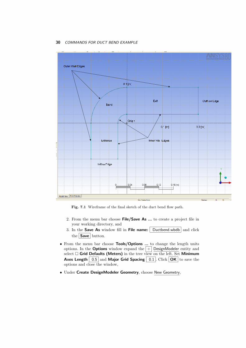
Fig. 7.1 Wireframe of the final sketch of the duct bend flow path.

2. From the menu bar choose File/Save As ... to create a project file inyour working directory, and

3. In the Save As window fill in File name: Ductbend.wbdb and clickthe Save button.

• From the menu bar choose Tools/Options ... to change the length unitsoptions. In the Options window expand the + DesignModeler entity andselect � Grid Defaults (Meters) in the tree view on the left. Set Minimum

Axes Length 0.5 and Major Grid Spacing 0.1 . Click OK to save theoptions and close the window,

• Under Create DesignModeler Geometry, choose New Geometry,

GEOMETRY MODEL 31

• Check that the desired length unit is © Meter is selected and click Ok inthe units window that appears,

• In the Tree View, select the XYPlane entity and then click the New Sketchicon to create the Sketch1 entity as a component of the XYPlane.

• To start the sketching , select the Sketching tab

• To draw in the 2D sketch of the duct flow path (Figure 7.1)

1. Select the Sketching tab; and2. Click on the Z coordinate of the triad in the lower right corner of the

Model View.• Select the Draw toolbox and:

1. With the Arc by Center tool sketch the inner wall bend shape:(a) Place the cursor over the origin (watch for the P constraint symbol)

and left mouse button click.(b) Move the cursor to the left along the X axis. With the C constraint

visible click the left mouse button to put the start point of the arcon the X axis.

(c) Sweep the cursor clockwise until the C constraint appears at the Yaxis. Click the left mouse button.2

2. Switch to the Dimensions toolbox to size the inner wall bend radius:(a) Select the Radius tool;(b) Select a point on the arc. Then move the cursor to the inside of the

arc near the origin. Click to complete a dimension which is labelledR1.

(c) In the Details View notice that R1 is shown under the Dimensionstitle.

(d) Change the value of R1 to 0.025 [m]. Notice the arc radius changesautomatically. If the dimension is poorly placed on your sketch youcan use the Move tool to correct the placement.

3. Switch back to the Draw toolbox to sketch the inner entrance wall:(a) With the Line tool selected, place the cursor in the lower left

quadrant of the XY plane near the arc. Click the left mouse button.Move the mouse cursor down to create a vertical line. Look for theV constraint symbol and click the left mouse button;

(b) Switch to the Dimensions toolbox to size the inner entrance walllength:i. Select the General tool;ii. Select a point near the centre of the line. Click and drag the cursor

to the right to form the dimension lines. Release the mouse buttonwhere the label, V2, is to be placed.

iii. In the Details View change the value of V2 to 0.10 [m].

2Notice that the drawing instruction steps are provided in the lower left corner.


(c) To join the inner entrance wall and the inner wall bend switch tothe Constraints toolbox;i. Select the Coincident tool;ii. Select the upper end of the entrance inner wall with a left mouse

button click. The square end marker should be yellow;iii. Select the square end marker of the arc that lies on the X axis

with a left mouse button click. The inner entrance wall shouldjoin the inner wall bend.

4. To draw a line across the inflow (entrance):(a) Use the Line tool in the Draw toolbox;(b) Place the cursor over the bottom end point of the entrance inner

wall and notice that a P constraint symbol appears. Left mousebutton click to select this point and then move the cursor to theleft and click while the H constraint symbol is visible.

(c) Use the General tool in the Dimensions toolbox:(d) Select a point near the centre of the line. Click and drag the cursor

to the bottom to form the dimension lines. Release the mouse buttonwhere the label, H3, is to be placed.

(e) In the Details View change the value of H3 to 0.075 [m].5. Repeat the procedure used for the entrance inner wall to draw the exit

inner wall:(a) Draw a horizontal line in the upper right XY quadrant near the end

point of the inner wall bend;(b) Set the length of the line to 0.20 [m] with the General tool from

the Dimensions toolbox;(c) Join the exit inner wall to the inner wall bend with the Coincident

tool from the Constraints toolbox.

6. Draw the outer entrance wall with the Line tool. Start at the outer(left) end point of the inflow edge (look for the P constraint symbol)and draw a vertical line that is coincident (C) with the X axis;

7. Draw the outer bend wall with the Arc by Center tool. Put the centreat the origin, make the start point at approximately 20◦ above the Xaxis in the upper left quadrant, and make the end point coincident (C)with the Y axis. Use the Coincident constraint tool to join the startpoint of the arc to the end point of the outer entrance wall;

8. Draw the outer exit wall with the Line tool. Draw a horizontal (H)line coincident (C) with the Y axis above its final desired location. Usethe Coincident constraint tool to join this line to the end of the outerbend wall. Use the Equal Length constraint tool to make the outerexit wall the same length as the inner exit wall; and

9. Draw a line from the end of the outer exit wall to the end of the innerexit wall to form the outflow edge. Make sure that the end points are

MESH GENERATION 33

coincident (P).The sketch should now be an enclosed contour on the XYPlane.

• To create the three dimensional solid body:1. Switch to the Tree View by selecting the Modeling tab;

2. Click on the Extrude button to create the Extrude1 feature . In theDetails View:∗ Check Base Object Sketch1 ,∗ Select Operation H Add Material ,

∗ Select Direction Vector H None (Normal) ,

∗ Set FD1, Depth (> 0) 0.02 ,∗ Select As Thin/Surface? H No , and∗ Select Merge Topology? H Yes .

3. Click on the Generate button to create a Solid. Use the isometric viewin the Model View to check that you have a three dimensional solid greybody.

• Choose File/Save As ... and set File name: Ductbend.agdb in the Save

As window. Click Save to close window.

• Return to the Project page by clicking on the Ductbend [Project] tab atthe top left corner of the window.

7.2 Mesh GenerationThe second phase uses CFX-Mesh. The commands listed below will generate adiscrete mesh in the flow domain:• name the surfaces (faces) of the solid geometry to ease boundary condition

specification;• specify the properties of the mesh in the interior of the flow domain and

close to solid walls;• preview the surface mesh to check for anomalies; and• create the geometry file with volume mesh information.

• Choose the Generate CFX Mesh DesignModeler Tasks; Notice the three pri-mary areas: Graphics View, Tree View, and Details View.

• The surfaces (faces) of the solid are labeled as regions for ease of attach-ing the boundary conditions . To attach a region entity at the inflow (seeFigure 7.1):1. Right mouse click over Regions in the Tree View and select Insert H

Composite 2D Region to create a new region entity;2. Left click over the new entity’s name, Composite 2D Region 1, and edit

the region name to inflow surface;3. In the Graphics View put the mouse cursor over the inlet surface area

and left mouse click. The inlet surface area should turn green; and


4. In the Details View click on Location H Apply ;

• Repeat to create a region entity called outflow surface. Notice that if youleft mouse button click on inflow surface or the outflow surface in the TreeView that the resulting region in the Graphics View turns green.

• Create a region entity called inner wall. This region is composed of threeprimitive surfaces. To select a set of surfaces or faces hold the ”Ctrl” keydown while clicking on the component surfaces in the Graphics View;

• Repeat to create an entity called outer wall;• For a region called front surface use the Z view of the Graphics View when

selecting the surface. Notice that there are two parallel planes in the lowerleft corner of the Graphics View. The front most of these planes should beoutlined in red.

• Do not set up a region for the back surface. It will remain as the singlesurface in the Default 2D Region.

• In the Tree View, select Options to see the mesh options in the Details View:

∗ Set Surface Meshing H Advancing Front ,

∗ Set Meshing Strategy H Extruded 2D Mesh ,

∗ Set 2D Extrusion Option H Full , and∗ Set Number of Layers H 1 ;

• In the Tree View, expand the + Spacing entity;• Select the Default Body Spacing entity to open the Body Spacing Details

View. Set Maximum Spacing [m] 0.0075 .• Left mouse click on the Extruded Periodic Pair entity;

∗ In the Graphics View select the front surface and then click Location

1 Apply in the Details View;∗ In the Graphics View select the back surface (remember to use the

location planes in the lower left corner of the Graphics View) and thenclick Location 2 Apply in the Details View; and

∗ Set Periodic Type H Translational ;• In the Tree View, right mouse click on Inflation and select Insert/Inflated

Boundary to create an Inflated Boundary entity. Select the three surfacesof the inner wall in the Graphics View for the Location and set MaximumThickness [m] 0.0075 ;

• Repeat to create an Inflated Boundary of Maximum Thickness [m] 0.0075on the outer wall;

• In the Tree View expand the + Preview entity. Right mouse click onDefault Preview Group and select Generate This Surface Mesh. Progressis shown in the lower left corner. After a short time you should see a meshof triangles and rectangles on the surfaces of the solid;

PRE-PROCESSING 35

• Click the Generate the volume mesh for the current problem icon on the

top row of icons/buttons. In the Windows file window set File name: Ductbend.gtm .Again, progress is shown in the lower left corner. When this process is com-pleted, go to the Tree View and select Errors to ensure that no errors arereported in the Details View.

• To close this phase, select File/Save As ... and set File name: Ductbend.cmdb .

• Return to the Project page by clicking on the Ductbend [Project] tab atthe top left corner of the window.

7.3 Pre-processingThe first CFD phase is preprocessing. In this phase the complete CFD model(mesh, fluids, flow processes, boundary conditions, etc.) is defined and saved ina hierarchical database. After opening CFX-Pre, the commands listed below willaccomplish the following steps:• link the mesh gtm file to a CFX flow project,• set simulation type to steady state,• establish a fluid with nominal properties of water,• specify the region through which the fluid will flow, the fluid (nominally

water), and the physical models (fluid flow, no heat transfer, turbulence,standard k − ε model with scalable wall functions),

• set up and attach the rough wall boundary condition, the inlet boundarycondition, the outlet boundary condition, and the symmetry boundary con-ditions,

• set the global initial conditions,• set the solver controls for discretization scheme, time step type, and conver-

gence criteria,• set the output variable list, and• write the complete CFD model definition to a def file.To accomplish these steps execute the following commands:• Highlight the mesh file, Ductbend.gtm, in the Project page and double click;• After a short wait the CFX-Pre page will open. This page is similar to

the CFX-Post page. There are three main areas: the menus and commandbuttons at the top, the Viewer window at the right, and the database panelsat the left;

• Select the Regions tab to see the region database:∗ Check that � Assembly entity under the Mesh Assemblies tree is on.

Click on the name of the entity, Assembly, to see the mesh on the ductwireframe model;

∗ To see the mesh on an individual region click the named regions in theComposite Regions tree. Click through each region in the tree;

∗ Expand + the inner wall and + the Union regions to see the threeprimitive faces that make up the region. Each primitive face has a name


of the form Fx.By - face x of body y where only the leading letter (For B) is shown.

∗ The (back surface was imported into CFX-Pre attached to the De-fault 2D Region. If you would like to correct this naming anomaly clickCreate New Object icon on the right of the Region panel. A small

New Region panel will open. Fill in Name back surface (assumingthat this is the missing surface) and click OK to open the RegionEditor panel will open up where you set:◦ Combination Alias

◦ Dimension H All◦ Select Default 2D Region to put into the Region List panel list; and◦ Click Ok to close panel.

• Click Materials tab in the database panel to open up a list of availablematerials. To define a new material click the Create New Object icon. In

the Create Material panel, fill in Name Water nominal and click OK toopen a panel with two tabs:∗ Click the Basic Settings tab and set:

∗ Option H Pure Substance ,

∗ Material Group H Constant Property Liquids ,∗ � Material Description off,∗ � Thermodynamic State on and Thermodynamic State H Liquid .

∗ Click the Material Properties tab and set:

∗ Option H General Material ,∗ expand Equation of State + ,

∗ Option H Value ,

∗ Density 1000 H kgm−3 ,

∗ expand Transport Properties + ,

∗ � Dynamic Viscosity on and Dynamic Viscosity 0.001 H Pa · s ,

and then click Ok .

• On the row of menu buttons, click the Define the Simulation Type button

to open the Simulation Type panel. Check that Option H Steady State is

set and then click Ok .

• Click the Create a Domain button. A small Create Domain definitionpanel will open. Fill in Name Ductbend and click OK to define thedomain object. An Edit Domain: Ductbend panel will open with severaltabbed sub-panels.∗ On the General Options sub-panel, set:

PRE-PROCESSING 37

◦ Location H Assembly ,

◦ Domain Type H Fluid Domain ,◦ Fluids List H Water nominal ,◦ � Particle Tracking off,◦ Reference Pressure 1 H atm ,◦ Buoyancy Option H Non Buoyant , and

◦ Domain Motion Option H Stationary .

∗ on the Fluid Models sub-panel set:◦ Heat Transfer Model Option H None ,◦ Turbulence Model Option H k-Epsilon ,

◦ Turbulent Wall Functions Option H Scalable ,◦ Reaction or Combustion Model Option H None , and◦ Thermal Radiation Model Option H None ,

∗ on the Initialization sub-panel ensure that � Domain Initialization

is off and then click Ok to close the panel. Notice that the Domain:

Ductbend is now listed in the Physics database tree. If you double-clickon this object in the list then the Edit panel will reappear.

• Click the Create a Boundary Condition button to open a definition panel.

Fill in Name INFLOW SURFACE and click OK . In the Edit Boundary:Inflow surface in Domain: Ductbend panel:

∗ under the Basic Settings tab set:

◦ Boundary Type H Inlet , and◦ Location H inflow surface ,

∗ and under the Boundary Details tab set:

◦ Flow Regime Option H Subsonic ,◦ Mass and Momentum Option H Normal Speed ,

◦ Normal Speed H 3 H ms−1 ,◦ Turbulence Option H Intensity and Length Scale ,

◦ Value 0.05 ,◦ Eddy Length Scale 0.0075 H m ,

and then click Ok to close the panel and create the new boundary ob-ject. Notice that incoming arrows appear on the inlet surface in the Viewer

window and the boundary object is listed in the Physics database tree.

Clicking on Boundary: INFLOW SURFACE object in the Physics

database causes the inflow surface mesh to be outlined with green in theViewer window.


• Click the Create a Boundary Condition button to open the definition

panel. Fill in Name OUTFLOW SURFACE and click OK . In the EditBoundary: Outflow surface in Domain: Ductbend panel:


◦ Boundary Type H Outlet , and◦ Location H outflow surface ,


◦ Flow Regime Option H Subsonic ,◦ Mass and Momentum Option H Average Static Pressure ,

◦ Relative Pressure 0 H Pa ,

and then click Ok to close the panel and create the new boundary object.


panel. Fill in Name FRONT SURFACE and click OK . In the Edit Bound-ary: Front Surface in Domain: Ductbend panel:


◦ Boundary Type H Symmetry , and

◦ Location H front surface ,



panel. Fill in Name BACK SURFACE and click OK . In the Edit Bound-ary: Back surface in Domain: Ductbend panel:


◦ Boundary Type H Symmetry , and

◦ Location H back surface ,



panel. Fill in Name INNER WALL and click OK . In the Edit Bound-ary: Inner wall in Domain: Ductbend panel:


◦ Boundary Type H Wall , and◦ Location H inner wall ,


◦ Wall Influence on Flow Option H No Slip ,◦ � Wall Velocity off,◦ Wall Roughness Option H Rough Wall ,

PRE-PROCESSING 39

◦ Roughness Height 0.0001 H m ,



panel. Fill in Name OUTER WALL and click OK . In the Edit Boundary:Outer wall in Domain: Ductbend panel:∗ under the Basic Settings tab set:

◦ Boundary Type H Wall , and◦ Location H outer wall ,


◦ Wall Influence on Flow Option H No Slip ,◦ � Wall Velocity off,◦ Wall Roughness Option H Rough Wall ,

◦ Roughness Height 0.0001 H m ,


• Click on the Define the Global Initial Conditions button to open the ini-tialization panel. Make sure that � Turbulence Eddy Dissipation is on. Youcan accept H Automatic initialization for all properties and click Ok .

• Click on the Define the Solver Control Criteria button to open the panel.Under the Basic Settings tab set:

∗ Advection Scheme Option H Upwind ,

∗ Timescale Control H Physical Timescale ,

∗ Physical Timescale 0.04 H s (30% of the average residence time ofa fluid parcel inside the flow domain),

∗ Max No. Iterations 50 ,

∗ Residual Type H MAX ,∗ Residual Target 1.0e-3 ,

and then click Ok .

• Click the Create Output Files and Monitor Points button to open the

panel. In the Results tab panel set:

∗ Option H Standard ,

∗ � Output Variable Operators on and choose H All , and

∗ � Output Boundary Flows on and choose H All ,

and then click Ok .

• Click the Write Solver File to open the panel. Accept the default filename,Ductbend.def and Operation H Start Solver Manager .


7.4 Solver ManagerThe CFX-Solver window will open after CFX-Pre closes. In the Define Runpanel set:

• Definition File ductbend.def (NOTE: If restarting a partially convergedrun, you would enter the name of the most current results file),

• Type of Run H Full , and

• Run Mode H Serial ,

and then click Start Run .After a few minutes execution should begin. Diagnostics will scroll on the ter-

minal output panel and the equation RMS residuals will be plotted as a functionof time step. After the first few time steps, the residuals should fall monotoni-cally. Execution should stop within 40 time steps. In the CFX-5 Solver Finished

Normally window click OK .

7.5 Post-processingThe most interesting step is the analysis of the results. To illustrate this step thecommands listed in the next paragraph step through the following tasks:• load the results from the res file for post-processing,• create a vector plot on one of the symmetry boundary planes,• save an image of the plot,• create a vorticity variable,• create a fringe plot of the vorticity field,• create a line and export the velocity data along the line,• export the inner wall pressure and wall shear stress distribution,• probe the velocity field, and• save the visualization state.To accomplish these tasks click the CFX-Post tab in bottom left corner and

then:• Choose File/Load Results, and select the Ductbend 001.res results file.• Choose Create/Vector, accept Name Vector 1 , and click OK to define

a vector object and open an edit panel. In the panel set:∗ Locations H FRONT SURFACE ,

∗ Reduction Reduction Factor ,∗ Factor 1 (plots vector at every mesh point),

∗ Variable H Velocity ,∗ © Hybrid on,∗ Projection H None ,∗ � Visibility on

and click Apply . The vector plot should appear in the Viewer window andthe vector object is listed in the Object database panel. Under the View

POST-PROCESSING 41

Control branch in the Object tree, turn � DEFAULT LEGEND off andback on to remove and then replace the scale legend. Under the Regionsbranch turn � Wireframe on. Orthographic projection will work best fortwo-dimensional views. Notice that if you double-click on an object in theObject tree then an edit panel opens up for that object.

• Choose File/Print ... and in the Print panel set:

∗ File vectorplot.png , and

∗ Format H PNG

followed by Print . The plot will printed to the file vectorplot.png in yourworking directory. You can import this file into other documents.

• Choose Create/Variable and in the New Variable definition window setName Vorticity and click OK . In Vorticity edit panel (lower left):

∗ set Method H Expression ,∗ set © Scalar on,∗ fill in Expression Velocity v.Gradient X - Velocity u.Gradient Y , and

∗ click Apply .

• Choose Create/Contour, accept Name Contour 1 , and click OK to de-fine a fringe/contour plot object and open an edit panel. In the panel set:

∗ Locations H FRONT SURFACE ,

∗ Variable H Vorticity ,∗ � Visibility on

and click Apply . The fringe plot should appear in the Viewer window.

• Choose Create/Location/Line, accept Name Line 1 , and click OK todefine a line object and open an edit panel. Use Method H Two Points ,set Point 1 to (0.0,0.1,0.0), set Point 2 to (0.0,0.025,0.0), set the number ofsamples to 25, and click Apply to see the line (make sure that the visibilityof the contour plot, etc. is turned off).

• Choose File/Export ... to open the Export panel where you can:

∗ set File velocity.csv ,∗ select Line 1 from the Locations list,∗ set � Export Geometry Information on,∗ select (Ctrl key plus click) Velocity u and Velocity v from the Select

Variable(s) list, and∗ click Save to write the data to a file in a comma-separated format that

can be imported into a conventional spreadsheet program for plottingor further analysis. Notice that this file includes x, y, and z values.

• Choose Create/Location/Plane, accept Name Plane 1 , and click OK

to define a plane object and open an edit panel. Use Method H XY Plane


with Z = 0[m] and click Apply (set � Visibility off to avoid clutter in theview).

• Choose Create/Location/Polyline, accept Name Polyline 1 , and click OK

to define a polyline object. In the edit panel use Method H Boundary Intersection

with Boundary List H INNER WALL and Intersect With H Plane 1 andthen click Apply . This creates a line that follows the inner wall. You canfollow the steps for export along a line to export the values of the pres-sure, total pressure, and wall shear (stress) along this line into the data filewall.csv.

• Choose Create/Location/Point, accept Name Point 1 , and click OK

to define a point object. Use Method H XYZ and initialize the point to(0.10,0.04,0) before clicking Apply . Choose Tools/Function Calculator to

open the Function Calculator panel. Use Function H probe , Location H

Point 1 , Variable H Velocity u.Gradient X (Note: Use the ... to get a

list of all possible variables.) before clicking on the Calculate button. Theresult with units appears in the Result box. Move the point around to probeother regions in the flow.

• Choose File/Save State and enter tutorial1.cst for the file name to saveall of the information associated with the visualization and post-processingobjects you have created in this session. You can load this state file (File/LoadState) to recreate these objects and images in later sessions. This facilityallows easy comparison of results between simulations.

• Return to the Project page and choose File/Exit. Select Yes to save high-lighted files.

7.6 Clean Up

The last step is to remove unnecessary files created by CFX-5. This step isnecessary to ensure that you do not exceed your disk quota. At the end of eachsession3 delete all files except:• *.agdb, *.cmdat, *.cmdb, *.wbdb, *.def and * *.res files.If you no longer need your results but would like to be able to replicate them

then you should delete all files except:• *.def files.After removing all unnecessary files, use the WinZip utility to compress the

contents of your directory.

3If you have used a local temp drive, remember to copy your work to your N: drive

ME 566 Computational Fluid Dynamics for Fluids...

Documents

Transcript of ME 566 Computational Fluid Dynamics for Fluids...