mclust Version 4 for R: Normal Mixture Modeling for …...mclust Version 4 for R: Normal Mixture...

mclust Version 4 for R: Normal Mixture Modeling forModel-Based Clustering, Classification, and Density Estimation

Chris Fraley, Adrian E. RafteryUniversity of Washington, USA

T. Brendan MurphyUniversity College Dublin, Ireland

Luca ScruccaUniversita degli Studi di Perugia, Italy

Technical Report No. 597

Department of StatisticsUniversity of Washington

Box 354322Seattle, WA 98195-4322 USA

June 2012

mclust is a contributed R package for model-based clustering, classification, and density estima-tion based on finite normal mixture modeling. It provides functions for parameter estimation viathe EM algorithm for normal mixture models with a variety of covariance structures, and func-tions for simulation from these models. Also included are functions that combine model-basedhierarchical clustering, EM for mixture estimation and the Bayesian Information Criterion (BIC)in comprehensive strategies for clustering, density estimation and discriminant analysis. Thereis additional functionality for displaying and visualizing the models along with clustering, clas-sification, and density estimation results. Several features of the software have been changed inthis version, in particular the functionality for discriminant analysis and density estimation hasbeen largely expanded. mclust is licensed under the GPL and distributed through CRAN; seehttp://cran.r-project.org/web/packages/mclust/index.html.

1

http://cran.r-project.org/web/packages/mclust/index.html

Contents

1 Overview 4

2 Model-Based Cluster Analysis 42.1 Basic Cluster Analysis Example using Mclust . . . . . . . . . . . . . . . . . . . . . . . . . . . . . . . . 42.2 mclustBIC and its summary function . . . . . . . . . . . . . . . . . . . . . . . . . . . . . . . . . . . . . 72.3 Extended Cluster Analysis Example . . . . . . . . . . . . . . . . . . . . . . . . . . . . . . . . . . . . . 92.4 Clustering Univariate Data . . . . . . . . . . . . . . . . . . . . . . . . . . . . . . . . . . . . . . . . . . 112.5 Regularizing with a Prior . . . . . . . . . . . . . . . . . . . . . . . . . . . . . . . . . . . . . . . . . . . 122.6 Clustering with Noise and Outliers . . . . . . . . . . . . . . . . . . . . . . . . . . . . . . . . . . . . . . 152.7 Further Considerations in Cluster Analysis . . . . . . . . . . . . . . . . . . . . . . . . . . . . . . . . . 16

3 EM for Mixture Models 173.1 Individual E and M Steps . . . . . . . . . . . . . . . . . . . . . . . . . . . . . . . . . . . . . . . . . . . 173.2 Uncertainty . . . . . . . . . . . . . . . . . . . . . . . . . . . . . . . . . . . . . . . . . . . . . . . . . . . 173.3 Control Parameters . . . . . . . . . . . . . . . . . . . . . . . . . . . . . . . . . . . . . . . . . . . . . . . 18

4 Bayesian Information Criterion 19

5 Model-Based Hierarchical Clustering 19

6 Density Estimation 21

7 Discriminant Analysis 237.1 Discriminant Analysis Through Eigenvalue Decomposition . . . . . . . . . . . . . . . . . . . . . . . . . 247.2 Model-based Discriminant Analysis via MclustDA . . . . . . . . . . . . . . . . . . . . . . . . . . . . . 287.3 Plotting methods . . . . . . . . . . . . . . . . . . . . . . . . . . . . . . . . . . . . . . . . . . . . . . . . 307.4 Classification of univariate data . . . . . . . . . . . . . . . . . . . . . . . . . . . . . . . . . . . . . . . . 31

8 Displays for Multidimensional Data 358.1 Displays for Bivariate Data . . . . . . . . . . . . . . . . . . . . . . . . . . . . . . . . . . . . . . . . . . 358.2 Displays for Higher Dimensional Data . . . . . . . . . . . . . . . . . . . . . . . . . . . . . . . . . . . . 37

8.2.1 Coordinate Projections . . . . . . . . . . . . . . . . . . . . . . . . . . . . . . . . . . . . . . . . 378.2.2 Random Projections . . . . . . . . . . . . . . . . . . . . . . . . . . . . . . . . . . . . . . . . . . 38

8.3 Dimension reduction for model-based clustering and classification . . . . . . . . . . . . . . . . . . . . . 398.3.1 Clustering . . . . . . . . . . . . . . . . . . . . . . . . . . . . . . . . . . . . . . . . . . . . . . . . 398.3.2 Classification . . . . . . . . . . . . . . . . . . . . . . . . . . . . . . . . . . . . . . . . . . . . . . 40

9 Combining Gaussian Mixture Components for Clustering 43

10 Simulation from Mixture Densities 47

11 Extensions 4711.1 Large Datasets . . . . . . . . . . . . . . . . . . . . . . . . . . . . . . . . . . . . . . . . . . . . . . . . . 4711.2 High-Dimensional Data . . . . . . . . . . . . . . . . . . . . . . . . . . . . . . . . . . . . . . . . . . . . 4811.3 Missing Data . . . . . . . . . . . . . . . . . . . . . . . . . . . . . . . . . . . . . . . . . . . . . . . . . . 48

12 Function Summary 4912.1 Hierarchical Clustering . . . . . . . . . . . . . . . . . . . . . . . . . . . . . . . . . . . . . . . . . . . . . 4912.2 Parameterized Gaussian Mixture Models . . . . . . . . . . . . . . . . . . . . . . . . . . . . . . . . . . . 4912.3 Density Computation for Parameterized Gaussian Mixtures . . . . . . . . . . . . . . . . . . . . . . . . 4912.4 Model-based Clustering . . . . . . . . . . . . . . . . . . . . . . . . . . . . . . . . . . . . . . . . . . . . 5112.5 Model-based Density Estimation . . . . . . . . . . . . . . . . . . . . . . . . . . . . . . . . . . . . . . . 5112.6 Discriminant Analysis . . . . . . . . . . . . . . . . . . . . . . . . . . . . . . . . . . . . . . . . . . . . . 5112.7 Bayesian Regularization . . . . . . . . . . . . . . . . . . . . . . . . . . . . . . . . . . . . . . . . . . . . 5112.8 Support for Modeling and Classification . . . . . . . . . . . . . . . . . . . . . . . . . . . . . . . . . . . 5112.9 Plotting Functions . . . . . . . . . . . . . . . . . . . . . . . . . . . . . . . . . . . . . . . . . . . . . . . 52

12.9.1 Other Plotting Functions . . . . . . . . . . . . . . . . . . . . . . . . . . . . . . . . . . . . . . . 52

2

A Appendix 53A.1 Clustering Models . . . . . . . . . . . . . . . . . . . . . . . . . . . . . . . . . . . . . . . . . . . . . . . 53A.2 Modeling Noise and Outliers . . . . . . . . . . . . . . . . . . . . . . . . . . . . . . . . . . . . . . . . . . 54A.3 Model Selection via BIC . . . . . . . . . . . . . . . . . . . . . . . . . . . . . . . . . . . . . . . . . . . . 54A.4 Adding a Prior to the Model . . . . . . . . . . . . . . . . . . . . . . . . . . . . . . . . . . . . . . . . . 54

List of Tables

1 Parameterizations of Σk currently available in mclust for multidimensional data. . . . . . . . . . . . . . 8

List of Figures

1 The bivariate faithful dataset. . . . . . . . . . . . . . . . . . . . . . . . . . . . . . . . . . . . . . . . . 52 Plots associated with Mclust for the faithful dataset. . . . . . . . . . . . . . . . . . . . . . . . . . . . 73 Maximum BIC values for the faithful dataset. . . . . . . . . . . . . . . . . . . . . . . . . . . . . . . . 94 The wreath dataset. . . . . . . . . . . . . . . . . . . . . . . . . . . . . . . . . . . . . . . . . . . . . . . 105 BIC for the wreath dataset. . . . . . . . . . . . . . . . . . . . . . . . . . . . . . . . . . . . . . . . . . . 116 Model for the wreath dataset. . . . . . . . . . . . . . . . . . . . . . . . . . . . . . . . . . . . . . . . . . 127 Model-based clustering for univariate data. . . . . . . . . . . . . . . . . . . . . . . . . . . . . . . . . . 138 Pairs plot of the trees dataset. . . . . . . . . . . . . . . . . . . . . . . . . . . . . . . . . . . . . . . . . 149 BIC with and without the prior. . . . . . . . . . . . . . . . . . . . . . . . . . . . . . . . . . . . . . . . 1510 Cluster analysis with noise. . . . . . . . . . . . . . . . . . . . . . . . . . . . . . . . . . . . . . . . . . . 1611 Uncertainty plot of the 3-cluster mixture model fit for the iris dataset. . . . . . . . . . . . . . . . . . 1812 Pairs plot of the iris dataset showing species. . . . . . . . . . . . . . . . . . . . . . . . . . . . . . . . 2013 Density estimate for the waiting time to next eruption from faithful dataset. . . . . . . . . . . . . . 2214 Density estimate diagnostics . . . . . . . . . . . . . . . . . . . . . . . . . . . . . . . . . . . . . . . . . . 2215 Density estimation for the faithful dataset. . . . . . . . . . . . . . . . . . . . . . . . . . . . . . . . . 2316 Scatterplot matrix with mixture components ellipses from MclustDA for the iris dataset. . . . . . . . 3117 Classification plots for pair of variables from MclustDA for the iris dataset. . . . . . . . . . . . . . . . 3218 Discriminant analysis for univariate simulated data. . . . . . . . . . . . . . . . . . . . . . . . . . . . . 3419 Classification and uncertainty plots for the faithful dataset. . . . . . . . . . . . . . . . . . . . . . . . 3520 Density and uncertainty surfaces for the Lansing Woods maples. . . . . . . . . . . . . . . . . . . . . . 3621 Coordinate projections for the iris dataset. . . . . . . . . . . . . . . . . . . . . . . . . . . . . . . . . . 3722 Random projections for the iris dataset. . . . . . . . . . . . . . . . . . . . . . . . . . . . . . . . . . . 3823 Plot of eigenvalues from MclustDR applied to a clustering model for the iris dataset. . . . . . . . . . . 4024 Scatterplot of clustering structure from MclustDR for the iris dataset. . . . . . . . . . . . . . . . . . . 4125 Contour plot of mixture densities (left) and uncertainty boundaries (right) from MclustDR for the iris

dataset. . . . . . . . . . . . . . . . . . . . . . . . . . . . . . . . . . . . . . . . . . . . . . . . . . . . . . 4226 Marginal mixture densities for the first two directions from MclustDR for the iris dataset. . . . . . . . 4227 Pairs plot for the first three dimensions from MclustDR for the banknote dataset. . . . . . . . . . . . . 4328 Contour plot of mixture densities for each class (left) and classification boundaries (right) from MclustDR

for the banknote dataset. . . . . . . . . . . . . . . . . . . . . . . . . . . . . . . . . . . . . . . . . . . . 4429 Solutions from combining mixture components for the ex4.1 dataset. . . . . . . . . . . . . . . . . . . . 4530 Entropy plots for combining mixture components for the ex4.1 dataset. . . . . . . . . . . . . . . . . . 4631 Data simulated from a model of the faithful dataset. . . . . . . . . . . . . . . . . . . . . . . . . . . . 4832 Missing data imputations. . . . . . . . . . . . . . . . . . . . . . . . . . . . . . . . . . . . . . . . . . . . 50

3

1 Overview

The mclust software [12, 14] currently includes the following features:

• Normal mixture modeling via EM for ten parameterized covariance structures;

• Simulation from parameterized Gaussian mixtures;

• Model-based clustering (covariance parameterization and number of clusters selected via BIC);

• Model-based hierarchical clustering for four covariance structures;

• Discriminant analysis based on finite mixture modeling (EDDA, MclustDA);

• Density estimation;

• Displays, including uncertainty plots, random projections, contour and perspective plots,classification plots, density curves in one and two dimensions;

• Combining Gaussian mixture components for clustering;

• Dimension reduction methods for model-based clustering and classification.

This manuscript describes Version 4 of mclust for R, with added functionality for displaying and vi-sualizing the models along with clustering, classification, and density estimation results. A numberof other aspects of the software have been changed as well, to reflect evolution in its use, in partic-ular the functionality for discriminant analysis and density estimation has been largely expanded.A comprehensive treatment of the methods used in mclust can be found in [13, 17, 31, 3].

mclust is licensed under the GPL and is available as the contributed package for the R language.It can be obtained from CRAN at http://cran.r-project.org/web/packages/mclust/index.html.Follow the instructions for installing R packages on your machine, and then do

> library(mclust)

inside the R console to use the software. Throughout this manual it will be assumed that thesesteps have been taken before running the examples.

Several contributed R packages have functions that require mclust including clustvarsel, fpc,prabclus, msir, and the Bioconductor package spotSegmentation [15]. A couple of tutorials onmclust have also been published [16, 18].

2 Model-Based Cluster Analysis

mclust provides functionality for cluster analysis combining model-based hierarchical clustering(section 5), EM for Gaussian mixture models (section 3), and BIC (section 4).

2.1 Basic Cluster Analysis Example using Mclust

As an illustration, consider the bivariate faithful dataset (included in the R language distribution)shown in Figure 1.

The following command performs a cluster analysis of the faithful dataset, and prints asummary of the results:

4

●

●

●

●

●

●

●

●

●

●

●

●

●

●

●

●

●

●

●

●

●

●

●

●

●

●

●

●

●●

●

●

●

●

●

●

●

●

●

●

●

●

●

●

●

●

●

●

●

●

●

●

●

●

●

●

●

●

●

●

●

●

●

●

●

●

● ●

●

●

●

●

●

●

●

●

●

●

●

●

●

●

●

●

●

●

●

●

●

●

●

●

●

●

●

●

●

●

●

●

●

●

●

●

●

●

●

●

●

●

●

●

●

●

●

●

●

●

●

●

●

●

●

●

●

●

●

●

●

●

●

●

●

●

●

●

●

●

●

●

●

●

●

●●

●

●

●

●

●

●●

●

●

●●

●

●

●

●

●

●

●

●

●

●

●

●

●

●

●

●

●

●

● ●

●

●

●

●

●

●

●●

●

●

●

●

●

●

●

●

●

●

●

●

●

●

●

●

●

●

●

●

●

●

●

●

●

●

●

●

●

●

●

●

●

●

●

●

●

●

●

●

●●● ●

●

●

●

●

●

●

●

●●

●

●

●

●

●

●

●

●

●

●

●

●

●

●

●

● ●

●

●

●

●

●

●●

●

●

●

●

●

●

●

●

●

●

●

1.5 2.0 2.5 3.0 3.5 4.0 4.5 5.0

5060

7080

90

eruptions

waiting

Figure 1: The bivariate faithful dataset.

> faithfulMclust <- Mclust(faithful)> summary(faithfulMclust)

----------------------------------------------------Gaussian finite mixture model fitted by EM algorithm----------------------------------------------------

Mclust EEE (elliposidal, equal volume, shape and orientation) model with 3 components:

log.likelihood n df BIC-1126.4 272 11 -2314.4

Clustering table:1 2 3

130 97 45

In this case, the best model according to BIC is an equal-covariance model with 3 components orclusters. A more detailed summary including the estimated parameters can be obtained with thefollowing code:

> summary(faithfulMclust, parameters = TRUE)


Mclust EEE (elliposidal, equal volume, shape and orientation) model with 3 components:

log.likelihood n df BIC

5

-1126.4 272 11 -2314.4


130 97 45

Mixing probabilities:1 2 3

0.46190 0.35646 0.18164

Means:[,1] [,2] [,3]

eruptions 4.4761 2.0378 3.8199waiting 80.8922 54.4935 77.6711

Variances:[,,1]

eruptions waitingeruptions 0.07728 0.4765waiting 0.47650 33.7485[,,2]

eruptions waitingeruptions 0.07728 0.4765waiting 0.47650 33.7485[,,3]

eruptions waitingeruptions 0.07728 0.4765waiting 0.47650 33.7485

The clustering results can be displayed as follows:

> plot(faithfulMclust)

The corresponding plots are shown in Figure 2.The covariance structures defining the models available in mclust are summarized in Table 1;

these models are explained in more detail in appendix A.1.The input to function Mclust includes the number of mixture components and the covariance

structures to consider. By default, Mclust compares BIC values for parameters optimized for up tonine components and all ten covariance structures currently available in the mclust software. Theoutput includes the parameters of the maximum-BIC model (where the maximum is taken over allof the models and numbers of components considered), and the corresponding classification anduncertainty.

The object produced by Mclust is a list with a components describing the estimated model.The names of these components can be displayed as follows:

> names(faithfulMclust)

[1] "call" "modelName" "n" "d"[5] "G" "BIC" "bic" "loglik"[9] "df" "parameters" "classification" "uncertainty"[13] "z"

and they are described in detail in the Mclust help file.

6

2 4 6 8

−400

0−3

500

−300

0−2

500

Number of components

BIC

●

●● ● ● ● ● ● ●

●

● ● ● ● ● ●

●

● ● ● ● ● ● ● ●

●

● ● ●● ● ●

●

●

●

●EIIVIIEEIVEIEVI

VVIEEEEEVVEVVVV

1.5 2.0 2.5 3.0 3.5 4.0 4.5 5.0

5060

7080

90

eruptionswa

iting

●

●

●

●

●●

●

●

●

●

●

●

●

●

●

●

●

●

●

●

●

●

●

●

●

●

●

● ●

●

●

●

●

●

●

●

●

●

●

●

●

●

●

●

●

●

●

●

●

●

●

●

●

●

●

●

●

●

●

●

●

●

●

●

●●

●●

●

●

●

●●

●

●

●

●

●

●

● ●

●●

●

●

●

●●

●

●

●

●

●●

●

●

●●

●

●

●

●

●

●

●

●● ●

●

●

●

●

●

●

●●

●

●

●

●

●

●

●●

●●

●

●

●

●

Classification

1.5 2.0 2.5 3.0 3.5 4.0 4.5 5.0

5060

7080

90

eruptions

waiti

ng

Classification Uncertainty

●

●

●

●

●

●

●

●

●

●

●

●

●

●

●

●

●

●

●

●

●

●

●

●

●

●

●

●

●

●

●

●

●

●

●

●

●

●

●

●

●

●

●

●

●

●

●

●

●

●

●

●

●

●

●

●

●

●

●

●

●

●

●

●

●

●

●

●

●

●

●

●

●

●

●

●

●

●

●

●

●

●

●

●

●

●

●

●

●

●

●

●

●

●

●

●

●

●

●

●

●

●

●

●

●

●

●

●

●

●

●

●

●

●

●

●

●

●

●

●

●

●

●

●

●

●

●

●

●

●

●

●

●

●

●

●

●

●

●

●

●

●

●

●

●

●

●

●

●

●

●

●

●

●

●

●

●

●

●

●

●

●

●

●

●

●

●

●

●

●

●

●

●

●

●

●

●

●●

●

●

●

●

●

●

●

●

●

●

●

● ●

●

●

●

●

●

●

●

●

●

●

●

●

●

●●

●

●●

●

●

●

●●

●

●

●

●

●

●

●

●

●

●

●

●

●

●

●

●

●

●

●

●●

●

●

●

●●●

●

●●

● ●

●

●

●

●

●

●

●

●

●

●

●

●

●●

●●

●

●

●

●

●●

●

●●

eruptions

waiti

ng

−30

−30

−25

−25

−20

−20

−15

−15

−10

−10

−5

−5

1.5 2.0 2.5 3.0 3.5 4.0 4.5 5.0

5060

7080

90log Density Contour Plot

Figure 2: Plots associated with the function Mclust for the faithful dataset with the default argu-ments. Clockwise from upper left: BIC, classification, uncertainty, density. The ellipses superimposed onthe classification and uncertainty plots correspond to the covariances of the components.

2.2 mclustBIC and its summary function

To do further analysis on the same dataset, for example to see the results for a different set ofmodels and/or different numbers of components, Mclust could be rerun. However this approachcould involve unnecessary repetition of computations and could also take considerable time whenthe dataset is large or the process is to be repeated many times. An alternative approach is to splitthe analysis into several parts using function mclustBIC.

For the faithful dataset, the following sequence of commands produces the same clusteringresult as the call to Mclust.

> faithfulBIC <- mclustBIC(faithful)> faithfulSummary <- summary(faithfulBIC, data = faithful)> faithfulSummary

7

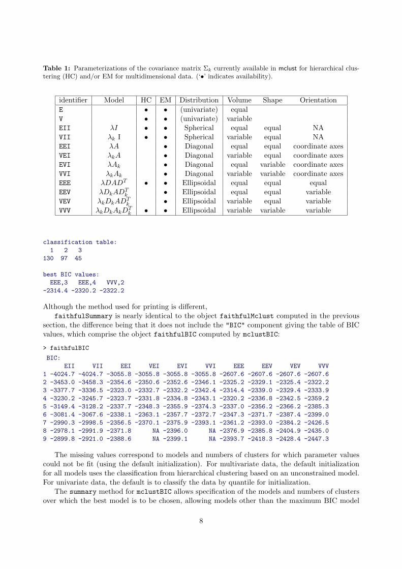
Table 1: Parameterizations of the covariance matrix Σk currently available in mclust for hierarchical clus-tering (HC) and/or EM for multidimensional data. (‘•’ indicates availability).

identifier Model HC EM Distribution Volume Shape OrientationE • • (univariate) equalV • • (univariate) variableEII λI • • Spherical equal equal NAVII λk I • • Spherical variable equal NAEEI λA • Diagonal equal equal coordinate axesVEI λkA • Diagonal variable equal coordinate axesEVI λAk • Diagonal equal variable coordinate axesVVI λkAk • Diagonal variable variable coordinate axesEEE λDADT • • Ellipsoidal equal equal equalEEV λDkADT

k • Ellipsoidal equal equal variableVEV λkDkADT

k • Ellipsoidal variable equal variableVVV λkDkAkDT

k • • Ellipsoidal variable variable variable

classification table:1 2 3

130 97 45

best BIC values:EEE,3 EEE,4 VVV,2

-2314.4 -2320.2 -2322.2

Although the method used for printing is different,faithfulSummary is nearly identical to the object faithfulMclust computed in the previous

section, the difference being that it does not include the "BIC" component giving the table of BICvalues, which comprise the object faithfulBIC computed by mclustBIC:

> faithfulBIC

BIC:EII VII EEI VEI EVI VVI EEE EEV VEV VVV

1 -4024.7 -4024.7 -3055.8 -3055.8 -3055.8 -3055.8 -2607.6 -2607.6 -2607.6 -2607.62 -3453.0 -3458.3 -2354.6 -2350.6 -2352.6 -2346.1 -2325.2 -2329.1 -2325.4 -2322.23 -3377.7 -3336.5 -2323.0 -2332.7 -2332.2 -2342.4 -2314.4 -2339.0 -2329.4 -2333.94 -3230.2 -3245.7 -2323.7 -2331.8 -2334.8 -2343.1 -2320.2 -2336.8 -2342.5 -2359.25 -3149.4 -3128.2 -2337.7 -2348.3 -2355.9 -2374.3 -2337.0 -2356.2 -2366.2 -2385.36 -3081.4 -3067.6 -2338.1 -2363.1 -2357.7 -2372.7 -2347.3 -2371.7 -2387.4 -2399.07 -2990.3 -2998.5 -2356.5 -2370.1 -2375.9 -2393.1 -2361.2 -2393.0 -2384.2 -2426.58 -2978.1 -2991.9 -2371.8 NA -2396.0 NA -2376.9 -2385.8 -2404.9 -2435.09 -2899.8 -2921.0 -2388.6 NA -2399.1 NA -2393.7 -2418.3 -2428.4 -2447.3

The missing values correspond to models and numbers of clusters for which parameter valuescould not be fit (using the default initialization). For multivariate data, the default initializationfor all models uses the classification from hierarchical clustering based on an unconstrained model.For univariate data, the default is to classify the data by quantile for initialization.

The summary method for mclustBIC allows specification of the models and numbers of clustersover which the best model is to be chosen, allowing models other than the maximum BIC model

8

to be extracted and analyzed.The plot method for mclustBIC allows specification of the models and numbers of clusters,

arguments to the legend function, as well as setting limits on the vertical axis. For example, thefollowing shows the maximum BIC values in more detail than the default:

> plot(faithfulBIC, G = 1:7, ylim = c(-2500,-2300), legendArgs = list(x = "bottomright", ncol = 5))

The resulting plot is shown in Figure 3.

1 2 3 4 5 6 7

−250

0−2

450

−240

0−2

350

−230

0


BIC

●

● ●

● ●

●

●

● ●

●

●

●

●

●●

● ●

●

●● ●

● ●

●

●

●

●

●

EIIVII

EEIVEI

EVIVVI

EEEEEV

VEVVVV

Figure 3: BIC plot for the faithful dataset, with vertical axes adjusted to display the maximum values.

2.3 Extended Cluster Analysis Example

As an example of an extended analysis, consider the wreath data shown in Figure 4. There are 1000bivariate observations simulated from a 14-component model in which the component covariancematrices are of equal size and shape, but differ in orientation.

> data(wreath)> plot(wreath, pch = 20, cex = 0.5)

The BIC values can be obtained with a call to mclustBIC and then plotted:

> wreathBIC <- mclustBIC(wreath)> plot(wreathBIC, legendArgs = list(x = "topleft"))

Refering to the BIC plot (shown on the left in Figure 5), the maximum BIC appears to be outsidethe range of the default values for the number of components in mclustBIC (and Mclust).

More components (for example, up to 20) can be considered in the analysis without recomputingprevious results:

> wreathBIC <- mclustBIC(wreath, G = 1:20, x = wreathBIC)> plot(wreathBIC, G = 10:20, legendArgs = list(x = "bottomright"))> summary(wreathBIC, wreath)

9

●

●

●

●

●

●

●

●

●

●

●

●

●

●

●

●

●

●

●

●●

●

●

●

●

●

●

●

●

●

●

●

●

●

●

●

●

●

●

●

●

●

●

●

●

●

●

●

●

●

●

●

●

●

●

●

●

●

●

●

●

●

●

●

●

●

●

●

●

●

●

●

●

●

●

●

●

●

●

●

●

●

●

●

●

●

●

●

●

●

●

●●

●

●

●

●

●

●

●

●

●

●

●

●●

●

●

●

●

●

●

●

●

●

●

●

●

●

●

●

●●

●

●

●

●

●

●

●

●

●

●

●

●

●

●

●

●

●

●

●

●

●

●

●

●

●

●

●

●

●

●

●

●

●

●

●

●

●

●

●

●

●

●

●

●

●

●

●

●

●

●

●

●

●

●

●

●

●

●

●

●●

●

●

●

●

●

●

●

●

●

●

●

●

●

●

●

●●

●

●

●

●

●

●

●

●

●

●

●

●

●

●

●

●

●

●

●

●

●

●

●

●

●

●

●

●

●

●

●

●

●

●

●

●

●

●

● ●

●

●

●

●

●

●

●

●

●

●

●

●

●

●

●

●

●

●

●

●

●

●

●

●

●

●

●

●

●

●

●

●

●

●

●

●

●

●

●

●

●

●

●

●

●

●

●

●

●

●

●

●

●

●

●

●

●

●

●

●

●

●

●

●

●

●

●

●

●

●

●

●

●

●

●

●

●

●

●

●

●

●

●

●

●

●

●

●

●

●

●

●

●

●

●

● ●

●

●

●

●

●

●

●

●

●

●

●

●

●

●●

●

●

●

●

●

●

●

●

●

●

●

●

●

●

●

●

●

●

●

●

●

●

●

●

● ●

●

●

●

●

●

●

●

●

●

●

●

●●

●

●

●

●

●

●

●

●

●

●

●

●

●

●

●

●

●

●

●

●

●

●●

●

●

●

●

●

●

●

●

●

●

●

●

●

●

●

●

●●

●

●

●

●

●

●

●

●

●

●

●

●

●

●

●

●

●

●

●

●

●

●

●

●

●

●

●●

●

●

●

●

●

●

●

●

●

●

●

●

●

●

●

●

●

●

●

●

●

●

●

●

●

●

●

●

●

●

●

●

●

●

●

●

●

●

●

●

●

●

●

●

●

●

●

●

●

●

●

●

●

●

●

●

●

●

●

●

●

●

●

●

●

●

●

●

●

●

●

●

●

●

●

●

●

●

●

●

●

●

●

●

●●

●

●

●

●

●

●

●

●

●

● ●

●

●

●●

●

●

●

●

●

●

●

●

●

●

●

●

●

●

●

●

●

●

●

●

●

●

●

●

●

●

●

●

●

●

●

●

●

●

●

●

●

●

●

●

●

●

●

●●

●

●

●

●

●

●

●

●

●

●

●

●

●

●

●

●

●

●

●

●

●

●

●

●

●

●

●

●

●●

●

●

●

●

●

●

●

●

●

●

●

●

●

●

●

●

●

●

●

●

●

●

●

●

●

●

●

●

●

●

●

●

●

●

●

●

●

●

●

●

●

●

●

●●

●

●

●

●

●

●

●

●

●

●

●

●

●

●

●

●

●

●

●

●

●

●

●

●

●

●

●

●

●

●

●

●

●

●

●

●

●

●

●

●

●

●

●

●

●

●

●●

●

●

●

●

●

●

●

●

●

●

●

●

●

●

●

●

●

●

●

●

●

●

●

●

●

●

●

●

●

●

●

●

●

●●

●

●

●

●

●

●

●

●

●

●

●

●

●

●

●●

●

●

●

●

●

●

●

●

●

●

●

●

●

●

●

●

●

●

●

●

●

●

●

●

●

●

●

●

●

●

●

●

●

●

●

●

●

●

●

●

●●

●

●

●

●

●

●

●

●

●

●

●

●

●

●

●

●

●

●

●

●

●

● ●

●

●

●

●●

●

●

●

●

●

●

●

●

●●

●

●

●

●

●

●

●

●

●

●

●

●

●

●

●

●

●

●

●

●

●

●

●

●

●

●

●

●

●

●

●

●

●

●

●

●

●

●

●

●

●

●

●

●

●

●

●

●

●

●

●

●

●

● ●

●

●

●

●

●

●

●

●

●

●

●

●

●

●

●

●

●

●

●

●

●

●

●

●

●

●

●

●

●

●

●

●

●

●

●

●

●

●

●

●

●

●

●

●

●

●

●

●

●

●

●

●

●

●

●

●

●

●

●

●

●

●

●

●

●

●

●

●

●

●

●

●

●

●

●

●

●

●●

●

●

●

●

●

−15 −10 −5 0 5 10 15

−10

010

wreath[,1]

wreath[,2]

Figure 4: The bivariate wreath dataset, which consists of 1000 observations simulated from a 14-componentnormal mixture in which the component covariance matrices are of equal size and shape, but differ inorientation.

classification table:1 2 3 4 5 6 7 8 9 10 11 12 13 1474 69 63 74 68 70 71 66 83 77 66 77 61 81

best BIC values:EEV,14 EEV,15 EEV,16-10903 -10926 -10953

The BIC plot is shown on the right in Figure 5. Using summary to obtain the best model according toBIC, a 14-component EEV model is chosen, which is in agreement with how the data was simulated.

> wreathModel <- summary(wreathBIC, data = wreath)> wreathModel


best BIC values:EEV,14 EEV,15 EEV,16-10903 -10926 -10953

The model for the wreath dataset is shown in Figure 6.The summary function can also be used to restrict the set of models and/or numbers of clusters

over which the best model is chosen according to BIC. For example, the following commands

10

2 4 6 8

−145

00−1

3500

−125

00


BIC

●

● ●

●

●●

● ●

●

●

●

●

●

●

●

● ●

●

●

●

●

●●

●

●

●

●

●

●

●

●

●

●

●

●

●

●

●

●

●

EIIVIIEEIVEIEVIVVIEEEEEVVEVVVV

10 12 14 16 18 20−150

00−1

4000

−130

00−1

2000

−110

00

Number of componentsBI

C

●

● ●

●

●●

● ●

●●

●

●

●

● ● ● ● ● ● ●

●

●

●●

●

●

● ●

●

●

●

●

●

● ● ● ●

●

●

●

●●

●

●

●

● ● ●●

●

● ● ● ●

●

●

●

●●

●

●

●

●

●

●

●

●

● ● ●

●

●

●

●

EIIVIIEEIVEIEVIVVIEEEEEVVEVVVV

Figure 5: BIC for wreath dataset. LEFT: BIC for all models and up to 9 components (the default inmclustBIC and Mclust). RIGHT: BIC for 10:20 components, all models. There is a clear peak for all modelsat 14 components.

produce the best spherical model for the wreath data:

> wreathSphericalModel <- summary(wreathBIC, data = wreath,modelNames = c("EII", "VII"))

> wreathSphericalModel


best BIC values:EII,14 EII,15 EII,16-11176 -11197 -11207

2.4 Clustering Univariate Data

Cluster analysis for univariate data can be carried out as for two and higher dimensions. As anexample, we use the precip dataset (included in the R language distribution):

> precipMclust <- Mclust(precip)> summary(precipMclust, parameters = TRUE)


Mclust V (univariate, unequal variance) model with 2 components:


Clustering table:

11

−15 −10 −5 0 5 10 15

−10

010

●

●

●●

● ●●

●●

●

●

●

●

●

●

●

●●

●●●

●●●●

●●●

●●

●●

●

●

●●

●●

● ●

●

●

●●

●●

●●●●

●

● ●●

●

●

●

●

●

●

●

●●

●●

●

●●

●

●

●●

●●

●●

●

●

●

●

●●

●

● ●

●

●

●●

●● ●

●

●

●●

●

●●

●

●

● ●●

●

●

●

●

●

●

●

●

●

●

●●●

●

●

●●●●

●

●

●

●

●

●

●

●

●

●

●●

●

●●

●

●

●

●●●

●

●●

●●

●●

●●

●●

●

●

●●

●

●

●

●

●

●

●

●●

●

●

●

●

●

●

●

●●●

●

●

●

●

●

●●

●

●

●

●

●

●●

●

●●

●

●

●

●●

●

●

●●

●

●

●

●●●●

●

●●

●

●●

●

● ●

●●

●●

● ●

●

●

●

●●

●

●

●

●

●●

●

●

●

●

●

●

●

●

●

●

●●

●

●

●●

●

●

●

●●

●

●

●●

●

●

●

●●

●

●●●●

●●

● ●

●

●

●

● ●●

●

●●

●

●●

●●

●

●●

●

●

●

●

●

●

●

●●

●

●●

●

●●●

●

●●

●

●● ●●

●

●●

●

●

●

●●

●

●

●● ●

● ●●●

●

●

●

●

●

●

●

●●●

●

●●● ●

● ●●● ●

●

●

● ●

●●

●

●

●● ●

●●

● ●●●

●

●●

●

●

●

●

●

●● ●

●

●

●●

●●

●●●

●

●

●●●●

●

●●

●

●

● ●●

●

●

●●● ●

●

●● ●●●

●

●

●

●

●

●

●

●

●●

●

●

●●●

●●●●

●●

●●

●

●●

●●

●●

●●●

● ●

●

●●●

●●

●●

●

●

●

●

●

●

●

●

●●

●

●●

●● ●

●

●●●

●

● ●●

●●

● ●●

●

●

●

●●

●●● ●

●

●●●

●

●●

●

●●●

●

●

●

●

● ●

●

●

●●

●

●

●

●

●

●

●

●

●

●

●●

●

●

●

●

●

●●●●

●●

●

●

●

●●

●●

●●

●

●

●

●●

●

●

●

●

●

●

●

●● ●●●

●

●

●

●

●●

●

●●●

●

●

● ●

●●

●

●

●

●

●●

●

●

●

● ●

●●

●●●

●

●

● ●●●

●

●●

●

●

●●

●

●●

●

●●

●●

●

●

● ●●

●

●

●

●●

●

●●

●

●●●●

●

●

●

●

●

●

●

●

●

●

●

●

●●●

●●

●●● ●

●

●

●

●●

●●

●●

●

●

●

●

● ●

●●

●

● ●●

●

●●

●●

●

●

●

●

●●

●

●● ●●

●

●●

●

●

●

●

●●●

●●

●

●●

●

●

●●

●

●

●

●

●●●●

●

●

●

●

●

●

●●

●

●

●

●

●

●●

●

●

●●

●

●

●

● ●●

●●

●● ●

●

●●

●

●

●

●

●●

●

●● ●●●

●

● ●

●

●

●●

●

●

●

●

●●

● ●

●●

●●●●●

●

●●

● ●●

●

●

●●●

●

●

●

●

●●

●●●

●

●

●●

●

●●

●

●●

●●

●

●

●

●

●

●

●

●

●●● ●

●

●

●

●●

●

●

●

●

●

●

●●

●●

●

●●●

●●

●●

●

●

●●●

●

● ●

●●

●

●

●

●

●

●● ●

●●

●

●

●

●

● ●●

●

●

●

●

●

●

●

●

●

●

●

●

●

● ●

●

●●

●

●

● ●

●

●

●

●

●

●●

●

●●

●

●

●

●

●●

●●

●

● ●

●

●

●

●

●●

●

●●

●

●

●

●

● ●

●

●● ●

●●

●

●

●

●●

●

●

●

●

●

●●

●

●

●

●

●

●

●

●●

● ●

●

●

●

●

●

●

●

●

●

●

●

●

●

●

●●

●● ●

●

●

●

●

●

●

● ●

●

Figure 6: The 14-component EEV (equal size and shape) model obtained for the wreath dataset.The ellipsessuperimposed on the plot correspond to the covariances of the components.

1 213 57

Mixing probabilities:1 2

0.18181 0.81819

Means:1 2

12.806 39.792

Variances:1 2

16.891 90.189

> plot(precipMclust, legendArgs = list(x = "bottomleft"))

Figure 7 shows the BIC, classification, uncertainty, and density for this example.

2.5 Regularizing with a Prior

mclust allows to specify a prior distribution to regularize the fit to the data [17]. We illustrate theuse of a prior on the trees dataset (included in the R language distribution), for which a pairs plot

12

2 4 6 8

−640

−630

−620

−610

−600

−590

−580

−570


BIC

EV

10 20 30 40 50 60

precip

12

Classification

| | ||| ||| || | ||

| | ||| ||| || | ||

|||| ||| | ||| || ||| | || |||||| |||| | || | | |||| || | || | || ||| || ||| || |

|||| ||| | ||| || ||| | || |||||| |||| | || | | |||| || | || | || ||| || ||| || |

10 20 30 40 50 60

0.0

0.2

0.4

0.6

0.8

1.0

precip

unce

rtain

ty

Uncertainty

10 20 30 40 50 60

0.00

00.

010

0.02

00.

030

precip

dens

ity

Density

Figure 7: Model-based clustering of the univariate R dataset precip. Clockwise from upper left: BIC,classification, uncertainty, and density from Mclust applied to the simulated univariate example. In theclassification plot, all of the data is displayed at the bottom, with the separated classes shown on differentlevels above.

is shown in Figure 8.The following commands compute and plot the BIC curves for the trees dataset provided in R

with and without a prior:

> treesBIC <- mclustBIC(trees) # default (no prior)> plot(treesBIC, legendArgs = list(x = "bottom", ncol = 2, cex = .75))> treesBICprior <- mclustBIC(trees, prior = priorControl())> plot(treesBICprior, legendArgs = list(x = "bottom", ncol = 2, cex = .75))

Without the prior, the BIC plot shows a number of jagged peaks, and many BIC values aremissing for some models due to failure in the EM computations caused by singularity and/orshrinking components. With the prior, the BICs are smoother and there are fewer failures inestimation. See Figure 9.

A function priorControl is provided in mclust for specifying the prior and its parameters.When called with its defaults, it invokes another function called defaultPrior which can serve asa template for specifying alternative priors. An example of the result of a call to defaultPrior isshown below.

> defaultPrior(trees, G=2, modelName = "VVV")

13

Girth

65 70 75 80 85

●●●

● ● ●● ● ●● ●●●●

●

● ●●

●● ● ●●

●●

● ●●●●

●

810

1214

1618

20

●●●

● ●●● ● ●● ●●●

●●

● ●●

●●●●●

●●

●●●●●

●

6570

7580

85

●

●

●

●

●

●

●

●

●

●

●

●●

●

●●

●●

●

●

●

●

●

●

●

●●

●●●

●

Height●

●

●

●

●

●

●

●

●

●

●

●●

●

●●

●●

●

●

●

●

●

●

●

●●

●●●

●

8 10 12 14 16 18 20

●●●

●●●

●●

●●

●

●●●●

●

●

●●●

●●

●●

●

●●●

●●

●

●●●

●● ●

●●

●●

●

●●●●

●

●

●●●

●●

●●

●

● ●●

●●

●

10 20 30 40 50 60 70

1020

3040

5060

70

Volume

Figure 8: Pairs plot of trees dataset.

$shrinkage[1] 0.01

$meanGirth Height Volume13.248 76.000 30.171

$dof[1] 5

$scaleGirth Height Volume

Girth 6.2038 6.5411 31.428Height 6.5411 25.5764 39.473Volume 31.4275 39.4733 170.217

For more detail on the prior and its specification, see Section A.4.

14

2 4 6 8

−700

−650

−600

−550


BIC

●

●●

●● ●

●

●●

●

●

●

●

●

●●

●

●●

● ●

●●

●

●

●

●

●

●

●

●

●

●

●EIIVIIEEIVEIEVI

VVIEEEEEVVEVVVV

2 4 6 8

−700

−650

−600

−550


BIC

●

●● ●

● ●

●

●

●

●

●●

●

●

●

●

●

●

●

●●

●

●

●

●●

●

●

●

●

●

●

●

●●

●

●

●

●

●EIIVIIEEIVEIEVI

VVIEEEEEVVEVVVV

Figure 9: BIC without (left) and with the prior (right) for the trees dataset.

2.6 Clustering with Noise and Outliers

mclust allows model-based clustering with noise, namely outlying observations that do not belongto any cluster. To include noise in the modeling, an initial guess of the noise observations must besupplied via the noise component of the initialization argument in Mclust or mclustBIC. Themodel for noise used in mclust is discussed in more detail in Section A.2 of the appendix, alongwith some some strategies for obtaining an initial noise estimate.

In the following example, Poisson noise is added to the faithful dataset. A random initialestimate was used for noise for the purposes of illustration. This happens to work well in thisinstance, although we don’t recommend this as a general strategy.

> b <- apply( faithful, 2, range)> nNoise <- 500> set.seed(0)> poissonNoise <- apply(b, 2, function(x, n)

runif(n, min = min(x)-.1, max = max(x)+.1), n = nNoise)> faithfulNdata <- rbind(faithful, poissonNoise)> set.seed(0)> faithfulNoiseInit <- sample(c(TRUE,FALSE),size=nrow(faithful)+nNoise,

replace=TRUE,prob=c(3,1))> faithfulNbic <- mclustBIC(faithfulNdata,

initialization = list(noise = faithfulNoiseInit))> faithfulNsummary <- summary(faithfulNbic, faithfulNdata)> faithfulNsummary

classification table:0 1 2

532 141 99

best BIC values:EVI,2 VVI,2 EEI,2

-7982.0 -7982.9 -7992.8

The results are shown in Figure 10. The classification and BIC plots were obtained with thefollowing commands.

15

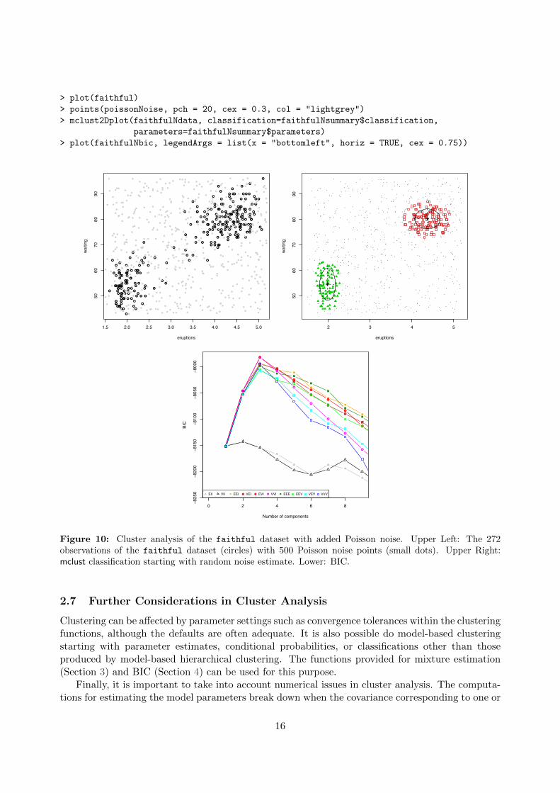
> plot(faithful)> points(poissonNoise, pch = 20, cex = 0.3, col = "lightgrey")> mclust2Dplot(faithfulNdata, classification=faithfulNsummary$classification,

parameters=faithfulNsummary$parameters)> plot(faithfulNbic, legendArgs = list(x = "bottomleft", horiz = TRUE, cex = 0.75))

●

●

●

●

●

●

●

●

●

●

●

●

●

●

●

●

●

●

●

●

●

●

●

●

●

●

●

●

●●

●

●

●

●

●

●

●

●

●

●

●

●

●

●

●

●

●

●

●

●

●

●

●

●

●

●

●

●

●

●

●

●

●

●

●

●

● ●

●

●

●

●

●

●

●

●

●

●

●

●

●

●

●

●

●

●

●

●

●

●

●

●

●

●

●

●

●

●

●

●

●

●

●

●

●

●

●

●

●

●

●

●

●

●

●

●

●

●

●

●

●

●

●

●

●

●

●

●

●

●

●

●

●

●

●

●

●

●

●

●

●

●

●

●●

●

●

●

●

●

●●

●

●

●●

●

●

●

●

●

●

●

●

●

●

●

●

●

●

●

●

●

●

● ●

●

●

●

●

●

●

●●

●

●

●

●

●

●

●

●

●

●

●

●

●

●

●

●

●

●

●

●

●

●

●

●

●

●

●

●

●

●

●

●

●

●

●

●

●

●

●

●

●●

● ●

●

●

●

●

●

●

●

●●

●

●

●

●

●

●

●

●

●

●

●

●

●

●

●

● ●

●

●

●

●

●

●●

●

●

●

●

●

●

●

●

●

●

●

1.5 2.0 2.5 3.0 3.5 4.0 4.5 5.0

5060

7080

90

eruptions

waiti

ng

●

●

●

●●

●

●

●

●

●

●

●

●

●

●●

●

●

●

●

●

●

●

●

●

●

●

●

●

●

●

●

●

●

●

●

●

●

●

●

●

●

●

●

●

●

●

●

●

●

●

●

●

●

●

●

●

●

●

●●

●

●

●

●

●

●

●

●

●

●

●

●

●

●

●

●

●

●

●

●

●

●

●

●

●

●

●

●

●

●

●

●

●

●

●

●

●

●

●

●

●

●

●

●

●●

●

●

●

●

●

●

●●

●

●

●

●

●

●

●

●

●

●

●

●

●

●

●

●

●

●

●

●

●

●

●

●

●

●

●

●

●

●

●

●

●

●

●

●

●

●

●

●

●

●

●

●

●

●

●

●

●

●

●

●

●

●

●

●

●

●

●

●

●

●

●

●

●

●

●

●

●

●

●

●

●

●

●

●

●

●

●

●

●

●

●

●

●

●

●

●

●

●

●

●

●

●

●

●●

●

●

●

●●

●

●

●

●

●

●

●

●

●

●

●

●

●

●

●

●

●

●

●

●

●

●

●

●

●

●

●

●

●

●

●

●

●

●

●

●

●

●

●

●

●

●

●

●

●

●

●

●

●

●

●

●

●

●

●

●

●

●

●

●

●

●

●

●

●

●

●

●

●

●

●

●

●

●

●

●

●

●

●

●

●

●

●

●

●

●

●

●

●

●

●

●

●

●

●

●

●

●

●

●

●●

●

●

●

●

●

●

●

●

●

●

●

●

●

●

●

●

●

●

●

●

●

●

●

●

●

●

●

●

●

●

●

●

●

●

●

●

●

●

●

●

●

●

●

●

●

●

●

●

●

●

●

●

●

●

●

●

●

●

●

●

●

●

●

●

●

●

●

●

●

●

●

●

●

●

●

●

●

●

●

●

●

●

●

●

●

●

●

●●

●

●

●

●

●

●

●

●

●

●

●

●

●

●

●

●

●

●

●

●

●

●

●

●

●

●

●

●

●

●

●

●

●

●

●

●

●

●

●

●

●

●

●

●

●

●

●

●

●

●

●

●

●

●

●

●

●

●

●

●

●

●

●

●

●

●

●

●

●

●

●

●

●

●

●

●

●

●

●

●

●

●

●

●

●

●

●

●

●

●

●

●

2 3 4 5

5060

7080

90

eruptions

waiti

ng

●

●

●

●

●

●

●

●

●

●

●

●

●

●

●

●

●

●

●

●

●

●

●

●

●

●

●

●●

●

●

●

●

●

●

●

●

●

●

●

●

●

●

●

●

●

●

●

●

●

●

●

●

●

●

●

●

●

●

●

●

●

●

●

●

●

●

●

●

●

●

●

●

●

●

●

●

●

●

● ●

●

●

●

●

●

●

●

● ●

●

●

●

●

●

●

●

●

●

●

●

●

●

●

●

●

●

●

●

●

●

●

●

●

●

●

●

●

●

●

●

●

●

●

●

●

●

●

●

●

●

●

●

●

●

●

●

●

●

●

●

●

●

●

●

●

●

●

●

●

●

●

●

●

●

●

●

●

●

●

●

●

●

●

●

●

●

●

●

●

●

●

●

●

●

●

●

●

●

●

●

●●

●

●

●

●

●

●●

●

●

●

●

●

●

●

●

●

●

●

●

●

●

●

●

●

●

●

●

●

●

●

●

●

●

●

●

●

●

●

●

●

●

●

●

●

●

●

●

●

●

●

●

●

●

●

●

●

●

●

●

●

●

●

●

●

●

●

●

●

●

●

●

●

●

●

●

●

●

●

●

●

●

●

●

●

●

●

●

●

●

●

●

●

●

●

●

●

●

●

●

●

●

●

●

●

●

●

●

●

●

●

●

●

●

●

●

●

●

●

●

●

●

●

●

●

●

●

●

●

●

●

●

●

●

●

●

●

●

●

●

●

●

●

●

●

●

●

●

●

●

●

●

●

●

●

●

●

●

●

●

●

●

●

●

●

●

●

●

●

●

●

●

●●

●

●

●

●

●

●

●

●

●

●

●

●

●

●

●

●

●

●

●

●

●

●

●

●

●

●

●

●

●

●

●

●

●

●

●

●

●

●

●

●

●

●

●

●

●

●

●

●

●

●

●

●

●

●

●

●

●

●

●

●

●

●

●

●

●

●

●

●

●

●

●

●

●

●

●

●

●

●

●

●

●

●

●

●

●

●

●

●

●

●

●

●

●●

●

●

●

●

●

●

●

●

●

●

●

●

●

●

●

●

●

●

●

●

●

●

●

●

●

●

●

●

●

●

●

●

●

●

●

●

●

●

●

●

●

●

●

●

●

●

●

●

●

●

●

●

●

●

●

●

●●

●

●

●

●

●

●

●

●

●

●

●

●

●

●

●

●

●

●

●

●

●

●

●

●

0 2 4 6 8

−825

0−8

200

−815

0−8

100

−805

0−8

000


BIC

●

●

●

●●

●

●

●

●

●

●

●

●

●

●

●

●

●

●

●

●

●

●

●

●

●

●

●

●

●

●

●

●

●

●

●

●

●

●

●

● ● ● ●EII VII EEI VEI EVI VVI EEE EEV VEV VVV

Figure 10: Cluster analysis of the faithful dataset with added Poisson noise. Upper Left: The 272observations of the faithful dataset (circles) with 500 Poisson noise points (small dots). Upper Right:mclust classification starting with random noise estimate. Lower: BIC.

2.7 Further Considerations in Cluster Analysis

Clustering can be affected by parameter settings such as convergence tolerances within the clusteringfunctions, although the defaults are often adequate. It is also possible do model-based clusteringstarting with parameter estimates, conditional probabilities, or classifications other than thoseproduced by model-based hierarchical clustering. The functions provided for mixture estimation(Section 3) and BIC (Section 4) can be used for this purpose.

Finally, it is important to take into account numerical issues in cluster analysis. The computa-tions for estimating the model parameters break down when the covariance corresponding to one or

16

more components becomes ill-conditioned (singular or nearly singular). Including a prior (SectionA.4) is often helpful in such situations. In general the modeling computations cannot proceed ifclusters contain only a few observations or if the observations they contain are very nearly colinear.Computations may also fail when one or more mixing proportions shrink to negligible values. TheEM functions in mclust compute and monitor the conditioning of the covariances, and an errorcondition is issued (unless such warnings are turned off) when the associated covariance appears tobe nearly singular, as determined by a threshold with the default value emControl()$eps.

3 EM for Mixture Models

mclust provides iterative EM (Expectation-Maximization) methods for maximum-likelihood estima-tion in parameterized Gaussian mixture models. In the models considered here, an iteration of EMconsists of an ‘E’-step, which computes a matrix z such that zik is an estimate of the conditionalprobability that observation i belongs to group k given the current parameter estimates, and an‘M’-step, which computes parameter estimates given z.

mclust functions em and me implement the EM algorithm for parameterized Gaussian mixtures.Function em starts with the E-step; besides the data and model specification, the model parameters(means, covariances, and mixing proportions) proportions must be provided. Function me startswith the M-step; besides the data and model specification, the conditional probabilities z must beprovided. The output for both are the maximum-likelihood estimates of the model parameters andz.

3.1 Individual E and M Steps

Functions estep and mstep implement the individual steps of the EM iteration. Conditionalprobabilities z and the log likelihood can be recovered from parameters via estep, while parameterscan be recovered from conditional probabilities z using mstep. Below we apply mstep and estep

to the iris dataset(included in the R language distribution).

> ms <- mstep(modelName = "VVV", data = iris[,-5], z = unmap(iris[,5]))> names(ms)

[1] "modelName" "prior" "n" "d" "G" "z"[7] "parameters"

> es <- estep(modelName = "VVV", data = iris[,-5], parameters = ms$parameters)> names(es)

[1] "modelName" "n" "d" "G" "z" "parameters"[7] "loglik"

In this example, the initial estimate of z for the M-step is a matrix of indicator variables correspond-ing to a discrete classification (iris[,5]). The function unmap converts a discrete classificationinto the corresponding indicator variables. mclust allows specification of a prior, for which the EMalgorithm will compute a posterior mode. See Sections 2.5 and A.4 for more details.

3.2 Uncertainty

The uncertainty in the classification associated with conditional probabilities z can be obtained bysubtracting the probability of the most likely group for each observation from 1:

> meVVViris <- me(modelName = "VVV", data = iris[,-5], z = unmap(iris[,5]))> uncer <- 1 - apply( meVVViris$z, 1, max)

17

The R function quantile applied to the uncertainty gives a measure of the quality of the classifi-cation:

> quantile(uncer)

0% 25% 50% 75% 100%0.0000e+00 0.0000e+00 1.9070e-08 1.3921e-03 3.3619e-01

In this case the indication is that the majority of observations are well classified. Note, however,that when groups intersect, uncertain classifications would be expected in the overlapping regions.

When a true classification is known, the relative uncertainty of misclassified observations canbe displayed by function uncerPlot, as is done below for the iris example (see Figure 11):

> uncerPlot(z = meVVViris$z, truth = iris[,5])

It is also possible to plot an uncertainty curve for one-dimensional data (see Section 2.4) or anuncertainty surface for bivariate data (see Section 8.1).

0.00

0.05

0.10

0.15

0.20

0.25

0.30

0.35

observations in order of increasing uncertainty

unce

rtain

ty

Figure 11: Uncertainty plot for the 3-cluster mixture model fit of the iris dataset via EM based onunconstrained Gaussian mixtures. The vertical lines indicate misclassified observations. The plot was createdwith function uncerPlot, and shows the relative uncertainty of misclassified observations.

3.3 Control Parameters

Besides the initial values and the prior, other parameters can influence the outcome of em or me.These include:

tol Iteration convergence tolerance. The default is emControl()$tol=c(1.e-5,√�M), where �M

is the relative machine precision, which has the value 2.220446e-16 on IEEE compliant

18

machines. The first value is the tolerance for relative convergence of the loglikelihood in theEM algorithm, and the second value is the relative parameter convergence tolerance for theM-step for those models that have an iterative M-step ("VEI", "VEV").

eps A tolerance for terminating iterations due to ill-conditioning, such as near singularity incovariance matrices. The default is emControl()$eps which is set to the relative machineprecision �M .

A function emControl is provided in mclust for setting these parameters and supplying defaultvalues. Although these control settings are in a sense hidden by the defaults, they may have asignificant effect on results in some instances and should be taken into consideration in analysis.

4 Bayesian Information Criterion

mclust provides a function bic to compute the Bayesian Information Criterion (BIC) [29] giventhe maximized loglikelihood for model, the data dimensions, and the number of components inthe model. The BIC is the value of the maximized log-likelihood with a penalty on the numberof model parameters, and allows comparison of models with differing parameterizations and/ordiffering numbers of clusters. In general the larger the value of the BIC, the stronger the evidencefor the model and number of clusters (see, e.g. [13]). The following shows the BIC calculation inmclust for the 3-cluster classification the iris dataset with the unconstrained variance model:

> meVVViris <- me(modelName = "VVV", data = iris[,-5], z = unmap(iris[,5]))> bic(modelName = "VVV", loglik = meVVViris$loglik,

n = nrow(iris), d = ncol(iris[,-5]), G = 3)

[1] -580.84

5 Model-Based Hierarchical Clustering

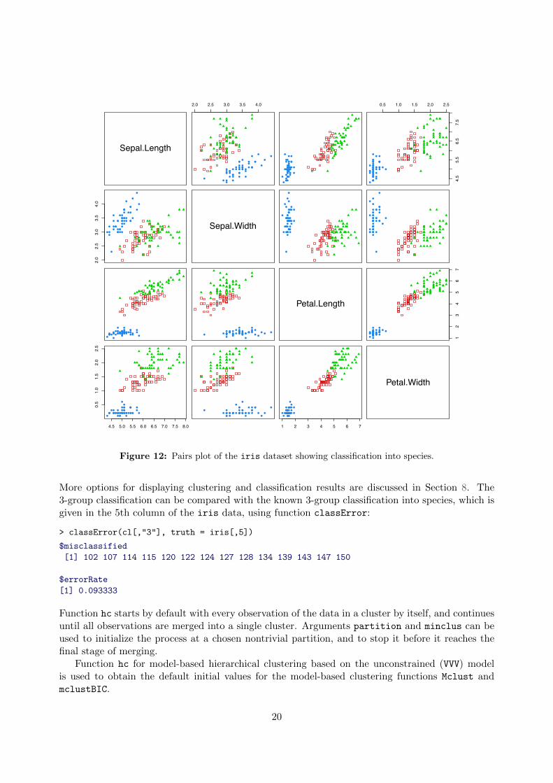
mclust provides functions hc for model-based hierarchical agglomeration, and hclass for determin-ing the resulting classifications. Function hc implements fast methods based on the multivariatenormal classification likelihood [10]. We use the iris dataset distributed with R in our example.Figure 12 is a pairs plot of the iris dataset in which the three species are differentiated by symbol,obtained by the following command:

> clPairs(data = iris[,-5], classification = iris[,5])

Below we apply the hierarchical clustering algorithm for unconstrained covariances (VVV) to theiris dataset:

> hcVVViris <- hc(modelName = "VVV", data = iris[,-5])

The classification produced by hc for various numbers of clusters can be obtained with hclass. Forexample, for the classifications corresponding to 2 and 3 clusters:

> cl <- hclass(hcVVViris, 2:3)

The classifications can be displayed with the data using clPairs:

> clPairs(data = iris[,-5], classification = cl[,"2"])> clPairs(data = iris[,-5], classification = cl[,"3"])

19

Sepal.Length

2.0 2.5 3.0 3.5 4.0

●

●

●●

●

●

●

●

●

●

●

●●

●

●●

●

●

●

●

●

●

●

●

●

● ●

●●

●●

●

●

●

●●

●

●

●

●●

●●

●●

●

●

●

●

●●

●

●●

●

●

●

●

●

●

●

●●

●

●●

●

●

●

●

●

●

●

●

●

●●

●●

●●

●

●

●

●●

●

●

●

●●

●●

●●

●

●

●

●

●

0.5 1.0 1.5 2.0 2.5

4.5

5.5

6.5

7.5

●

●

●●

●

●

●

●

●

●

●

●●

●

●●

●

●

●

●

●

●

●

●

●

● ●

●●

●●

●

●

●

●●

●

●

●

●●

●●

●●

●

●

●

●

●

2.0

2.5

3.0

3.5

4.0

●

●

●●

●

●

● ●

●

●

●

●

●●

●

●

●

●

●●

●

●●

●●

●

●●●

●●

●

●●

●●

●●

●

●●

●

●

●

●

●

●

●

●

● Sepal.Width●

●

●●

●

●

●●

●

●

●

●

●●

●

●

●

●

●●

●

●●

●●

●

●●●

●●

●

●●

●●

●●

●

●●

●

●

●

●

●

●

●

●

●

●

●

●●

●

●

●●

●

●

●

●

●●

●

●

●

●

●●

●

●●

●●

●

●●●

●●

●

●●

●●

●●

●

●●

●

●

●

●

●

●

●

●

●

●●●● ●

●

● ●● ● ●●●

● ●

●●●

●●

●●

●

●●

●● ●●●● ●● ●●

● ●●●●

●●●

●

●

●●

● ●● ●● ●● ●

●

●●● ● ●●●

● ●

●●●

●●

●●

●

●●

● ● ●●●● ● ● ●●

● ● ●●●

●● ●

●

●

●●

● ●●

Petal.Length

12

34

56

7

●●●●●

●

●●●● ●●●

● ●

●●●

●●

●●

●

●●

● ●●●●● ●● ●●

●●● ●

●●●●

●

●

●●●●●

4.5 5.0 5.5 6.0 6.5 7.0 7.5 8.0

0.5

1.0

1.5

2.0

2.5

●●●● ●

●●

●●●

●●●●

●

●●● ●●

●

●

●

●

● ●

●

●●●●

●

●●●● ●

●● ●

●●●

●

●●

●● ●● ●● ●● ●

●●●●

●●●

●●●

●●● ●●

●

●

●

●

●●

●

●●●●

●

●●● ● ●

●● ●

●●●

●

●●

●● ●●

1 2 3 4 5 6 7

●●●●●

●●●●●●●●●

●

●●● ●●

●

●

●

●

●●

●

●●●●

●

●●●●●●●●●●●

●

●●●●●●

Petal.Width

Figure 12: Pairs plot of the iris dataset showing classification into species.

More options for displaying clustering and classification results are discussed in Section 8. The3-group classification can be compared with the known 3-group classification into species, which isgiven in the 5th column of the iris data, using function classError:

> classError(cl[,"3"], truth = iris[,5])

$misclassified[1] 102 107 114 115 120 122 124 127 128 134 139 143 147 150

$errorRate[1] 0.093333

Function hc starts by default with every observation of the data in a cluster by itself, and continuesuntil all observations are merged into a single cluster. Arguments partition and minclus can beused to initialize the process at a chosen nontrivial partition, and to stop it before it reaches thefinal stage of merging.

Function hc for model-based hierarchical clustering based on the unconstrained (VVV) modelis used to obtain the default initial values for the model-based clustering functions Mclust andmclustBIC.

20

6 Density Estimation

The finite mixture estimation capabilities of mclust can also be viewed as a general strategy fordensity estimation.

Consider the following one-dimensional case:

> densWaiting <- densityMclust(faithful$waiting)> summary(densWaiting, parameters = TRUE)

-------------------------------------------------------Density estimation via Gaussian finite mixture modeling-------------------------------------------------------

Mclust E (univariate, equal variance) model with 2 components:

log.likelihood n df BIC-1034 272 4 -2090.4


Mixing probabilities:1 2

0.36102 0.63898

Means:1 2

54.619 80.094

Variances:1 2

34.439 34.439

A two-components mixture of Gaussian variables with the same variance is selected by BIC. Theparameter estimates can be read from the summary output.

A plot of density estimate can be obtained using the corresponding plot method:

> plot(densWaiting)

The density can also be plotted together with a histogram of the observed data by using the optionalargument data:

> plot(densWaiting, data = faithful$waiting)

In the one-dimensional case two diagnostic plots [24, pp. 87–90] for density estimation areavailable. The first plot is a graph of the estimated CDF vs the empirical distribution function(see left panel of Figure 14). The estimated CDF is computed by the function cdfMclust, whichnumerically integrate the density estimate over a grid of points. The second graph is a Q-Q plotof the sample quantiles vs the quantiles computed from the estimated density (see right panel ofFigure 14). Both graphs can be obtained as follows:

> plot(densWaiting, what = "diagnostic")

A plot of BIC values as discussed in Section 2 is also available by setting what = "BIC".Moving to higher dimensions, we may consider the bivariate faithful dataset:

21

40 50 60 70 80 90 100

0.00

0.01

0.02

0.03

0.04

faithful$waiting

Density

faithful$waiting

Density

40 50 60 70 80 90 100

0.00

0.01

0.02

0.03

0.04

Figure 13: Density estimate (left) and density estimate with histogram of data (right) for the waiting timeto next eruption from faithful dataset.

40 50 60 70 80 90 100

0.0

0.2

0.4

0.6

0.8

1.0

CDF plot

faithful$waiting

Cum

ulat

ive D

istri

butio

n Fu

nctio

n

Est.CDF Emp.CDF●●

●●●●●●●●●●●●●●●●●●●●●●●●●●●●●●●●●●●●●●●●●●●●●●●●●

●●●●●●●●●●●●●●●●●●●●●●●●

●●●●●●

●●●●●●●●●●●

●●●●●●●●●●●●●

●●●●●●●●●●●●●●●●●●●●●●●●●●●●●●●●●●●●●●●●●●●●●●●●●●●●●●●●●●●●●●●

●●●●●●●●●●●●●●●●●●●●●●●●●●●●●●●●●●●●●●●●●●●●●●●●●●●●●●●●●

●●●●●●●●●●●●●●●●●●●●●●●●●●●●●●●●●●●●●●●

●●●●

●

50 60 70 80 90

5060

7080

90

Q−Q plot

Quantiles from estimated density

Sam

ple

Qua

ntile

s

Figure 14: Density estimate diagnostics: plot of estimated CDF and empirical distribution function (left);Q-Q plot of sample quantiles vs quantiles from density estimation.

> faithfulDens <- densityMclust(faithful)

For two-dimensional data the default plot produces a contour plot of density estimates:

> plot(faithfulDens)> plot(faithfulDens, faithful, col = "grey", nlevels = 10, drawlabels = FALSE)

The two plots are shown in the top panels of Figure 15. In the second contour plot we added thesample data and we customize some parameters. A bivariate density estimate may also be plottedusing an image plot or a perspective plot as follows:

> plot(faithfulDens, type = "image", col = topo.colors(50))> plot(faithfulDens, type = "persp", col = grey(0.8))

The graphs are reported in the bottom panels of Figure 15.

22

eruptions

waiti

ng

0.005 0.005

0.01

0.01

0.015

0.015

0.02

0.02

0.025

0.025

0.03

0.03

0.03

5

0.04

1.5 2.0 2.5 3.0 3.5 4.0 4.5 5.0

5060

7080

90

eruptions

waiti

ng

1.5 2.0 2.5 3.0 3.5 4.0 4.5 5.0

5060

7080

90

●

●

●

●

●

●

●

●

●

●

●

●

●

●

●

●

●

●

●

●

●

●

●

●

●

●

●

●

●●

●

●

●

●

●

●

●

●

●

●

●

●

●

●

●

●

●

●

●

●

●

●

●

●

●

●

●

●

●

●

●

●

●

●

●

●

● ●

●

●

●

●

●

●

●

●

●

●

●

●

●

●

●

●

●

●

●

●

●

●

●

●

●

●

●

●

●

●

●

●

●

●

●

●

●

●

●

●

●

●

●

●

●

●

●

●

●

●

●

●

●

●

●

●

●

●

●

●

●

●

●

●

●

●

●

●

●

●

●

●

●

●

●

●●

●

●

●

●

●

●●

●

●

●●

●

●

●

●

●

●

●

●

●

●

●

●

●

●

●

●

●

●

● ●

●

●

●

●

●

●

●●

●

●

●

●

●

●

●

●

●

●

●

●

●

●

●

●

●

●

●

●

●

●

●

●

●

●

●

●

●

●

●

●

●

●

●

●

●

●

●

●

●●● ●

●

●

●

●

●

●

●

●●

●

●

●

●

●

●

●

●

●

●

●

●

●

●

●

● ●

●

●

●

●

●

●●

●

●

●

●

●

●

●

●

●

●

●

2.0 2.5 3.0 3.5 4.0 4.5 5.0

5060

7080

90

eruptions

waiti

ng

eruptions

waiting

Density

Figure 15: Contour, image and perspective plots of an mclust density estimate for the bivariate faithfuldataset.

Density estimation on more than two dimensions is straightforward with mclust. The onlydifficulty is found when we want to plot the estimated density. mclust takes a simple route, i.e.,it provides density (countour, image, and perspective) plots for all pairs of variables arranged in amatrix.

Finally, we note that the function dens is provided to easily get the density of a given set ofpoints relative to an estimated model. See help(dens) and the examples therein.

7 Discriminant Analysis

In discriminant analysis, observations of known classification are used to classify others. mclustprovides the function MclustDA which allows several approaches to discriminant analysis. Wedemonstrate some possible methods applied to the well-known iris dataset split into a trainingset and test set:

> odd <- seq(from=1, to=nrow(iris), by=2)> trainData <- iris[odd,1:4]

23

> trainClass <- iris$Species[odd]> testData <- iris[-odd,1:4]> testClass <- iris$Species[-odd]

7.1 Discriminant Analysis Through Eigenvalue Decomposition

Bensmail and Celeux [4] proposed the use of Gaussian finite mixture modeling for discriminantanalysis in which each known class is modeled by a single Gaussian term with the same covari-ance structure among classes. They named this procedure Eigenvalue Decomposition DiscriminantAnalysis or EDDA. This method for discriminant analysis is available as an option (named EDDA)in function MclustDA.

Consider the following model:

> irisEEE <- MclustDA(trainData, trainClass, modelType = "EDDA", modelNames = "EEE")> summary(irisEEE, parameters = TRUE)

------------------------------------------------Gaussian finite mixture model for classification------------------------------------------------

EDDA model summary:


Classes n Model Gsetosa 25 EEE 1versicolor 25 EEE 1virginica 25 EEE 1

Estimated parameters:

Class = setosa

Mixing probabilities: 1

Means:[,1]

Sepal.Length 5.024Sepal.Width 3.480Petal.Length 1.456Petal.Width 0.228

Variances:[,,1]

Sepal.Length Sepal.Width Petal.Length Petal.WidthSepal.Length 0.264181 0.062448 0.159355 0.031413Sepal.Width 0.062448 0.096309 0.033269 0.032224Petal.Length 0.159355 0.033269 0.182368 0.040917Petal.Width 0.031413 0.032224 0.040917 0.038912

Class = versicolor


24

Means:[,1]


Variances:[,,1]


Class = virginica


Means:[,1]


Variances:[,,1]


Training classification summary:

PredictedClass setosa versicolor virginicasetosa 25 0 0versicolor 0 24 1virginica 0 1 24

Training error = 0.026667

The above model fits a separate mean vector for each class, but the same ellipsoidal covariancematrix, which is essentially equivalent to linear discriminant analysis.

If we want to allow for different within-class covariance matrices (which is essentially equivalentto quadratic discriminant analysis) we can use:

> irisVVV <- MclustDA(trainData, trainClass, modelType = "EDDA", modelNames = "VVV")> summary(irisVVV, parameters = TRUE)

------------------------------------------------Gaussian finite mixture model for classification

25

------------------------------------------------

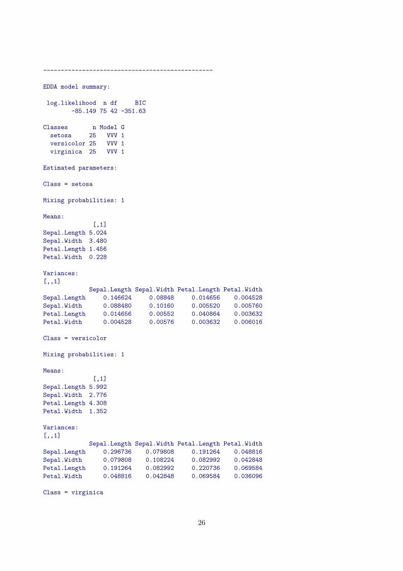
EDDA model summary:


Classes n Model Gsetosa 25 VVV 1versicolor 25 VVV 1virginica 25 VVV 1

Estimated parameters:

Class = setosa


Means:[,1]


Variances:[,,1]


Class = versicolor


Means:[,1]


Variances:[,,1]


Class = virginica

26


Means:[,1]


Variances:[,,1]





Other possible parameterization of the covariance matrix are reported in Table 1. If the ar-gument modelNames is not provided, the best model is chosen from among all available param-eterizations using the BIC. Most commonly in classification problems, model selection would bedone by computing the classification error using cross-validation or, if available, a test set. mclustprovides the function cv.MclustDA for computing k-fold cross-validation error, and the functionpredict.MclustDA for classifying new observations. With the above example data, we may com-pute the three statistics and compare the results as follows:

> models <- mclust.options()$emModelNames> tab <- matrix(NA, nrow = length(models), ncol = 3)> rownames(tab) <- models> colnames(tab) <- c("BIC", "10-fold CV", "Test error")> for(i in seq(models))

{mod <- MclustDA(trainData, trainClass,

modelType = "EDDA", modelNames = models[i])tab[i,1] <- mod$bictab[i,2] <- cv.MclustDA(mod, nfold = 10, verbose = FALSE)$errorpred <- predict(mod, testData)tab[i,3] <- classError(pred$classification, testClass)$errorRate

}> tab

BIC 10-fold CV Test errorEII -462.26 0.053333 0.066667VII -450.76 0.053333 0.066667EEI -417.16 0.053333 0.040000

27

VEI -401.31 0.040000 0.040000EVI -424.79 0.040000 0.040000VVI -398.00 0.040000 0.040000EEE -345.87 0.026667 0.040000EEV -347.45 0.026667 0.053333VEV -331.30 0.040000 0.040000VVV -351.63 0.026667 0.040000

The largest BIC is achieved by the VEV model, which is also one of the models with both thesmallest cross-validation error and test errror. Although in this case cross-validation, test error,and BIC happen to choose the same model, for other datasets the models selected, and hence thediscriminant results, could be different.

7.2 Model-based Discriminant Analysis via MclustDA

In Section 7.1, discriminant analysis was accomplished by modeling the training data with a mixturedensity having a single Gaussian component for each class. A more flexible alternative is to usemodel-based clustering to fit a Gaussian mixture model as a density estimate for each class in thetraining set [13].

In mclust this model can be fitted as follows:

> irisMCLUSTDA <- MclustDA(trainData, trainClass, modelType = "MclustDA")

For clarity of exposition we specified modelType = "MclustDA", but this argument can be omittedsince it is the default. Other arguments that could have been given are G, for the number ofmixture components, and modelNames, for the parameterization of class covariance matrix. If Gis not provided up to 5 components are fit for each class. If modelNames is not provided the bestmodel for each class is chosen from among all available parameterizations using the BIC. If providedas single vector of values, for example

> MclustDA(trainData, trainClass, modelType = "MclustDA",G = 1:2, modelNames = c("EII", "EEE"))

the search for the largest BIC values within each class is performed among the models EII and EEE,with one or two mixture components. Such arguments could also be supplied as lists, for example

> MclustDA(trainData, trainClass, modelType = "MclustDA",G = list(1:3, 1:2, 1), modelNames = list("EII", "EEE", c("EEE", "VVV")))

In this case, each pair of (i) number of mixture components and (ii) model name is used in fittingthe corresponding mixture model within each class. Thus, the first class is fitted with model EIIhaving from one to three components, the second class with model EEE having from one to twocomponents, and the last class with a single component mixture chosen between models EEE andVVV.

A fitted model can be summarized as follows:

> summary(irisMCLUSTDA)


MclustDA model summary:

28


Classes n Model Gsetosa 25 VEI 2versicolor 25 EEV 2virginica 25 XXX 1



Training error = 0

In this case BIC selects the VEI model with two components for the setosa Irises, the EEV modelwith two components for the versicolor Irises, and the single component with full covariance matrixfor the virginica Irises. The summary method prints also the confusion table and the error for thetraining data. The latter turns out to be zero, but a more realistic estimate of the classificationerror requires the evaluation of the fitted model in a cross-validated or test set.

The function cv.MclustDA can be used to obtain the k-fold cross-validation classification, errorrate, and standard error of classification:

> cv = cv.MclustDA(irisMCLUSTDA, nfold = 10, verbose = FALSE)> str(cv)

List of 3$ classification: Factor w/ 3 levels "setosa","versicolor",..: 1 1 1 1 1 1 1 1 1 1 ...$ error : num 0.04$ se : num 0.0194

Given a test data set and the corresponding classes for the observations in the test set, the testerror rate is obtained as follows:

> pred <- predict(irisMCLUSTDA, testData)> classError(pred$classification, testClass)$errorRate

[1] 0.013333

Alternatively, the summary method could be used to obtain the test error rate:

> summary(irisMCLUSTDA, newdata = testData, newclass = testClass)




Classes n Model G

29

setosa 25 VEI 2versicolor 25 EEV 2virginica 25 XXX 1



Training error = 0

Test classification summary:


Test error = 0.013333

7.3 Plotting methods

Several plots for discriminant analysis objects are available throught the plot method. Here weillustrate a subset of them, inviting the interested reader to consult help(plot.MclustDA) for amore comprehensive list and examples.

The default plot, corresponding to the omitted argument what = "scatterplot", is obtainedas:

> plot(irisMCLUSTDA)

and it is shown in Figure 16. This produces a scatterplot matrix for pairs of variables with pointsmarked according to the corresponding class, and mixture components ellipses superimposed. Asubset of variables can be selected with the argument dimens, for instance:

> plot(irisMCLUSTDA, dimens = 3:4)

A plot of data points, either from train set and from test set, marked according the known orestimated classification is easily obtained as:

> plot(irisMCLUSTDA, what = "classification", dimens = 3:4)> plot(irisMCLUSTDA, what = "classification", newdata = testData, dimens = 3:4)

where we selected only the third and fourth variable to plot. The resulting graphs are shown in toppanels of Figure 17.

Two other available displays are:

> plot(irisMCLUSTDA, what = "train&test", newdata = testData, dimens = 3:4)> plot(irisMCLUSTDA, what = "error", newdata = testData, newclass = testClass, dimens = 3:4)

30

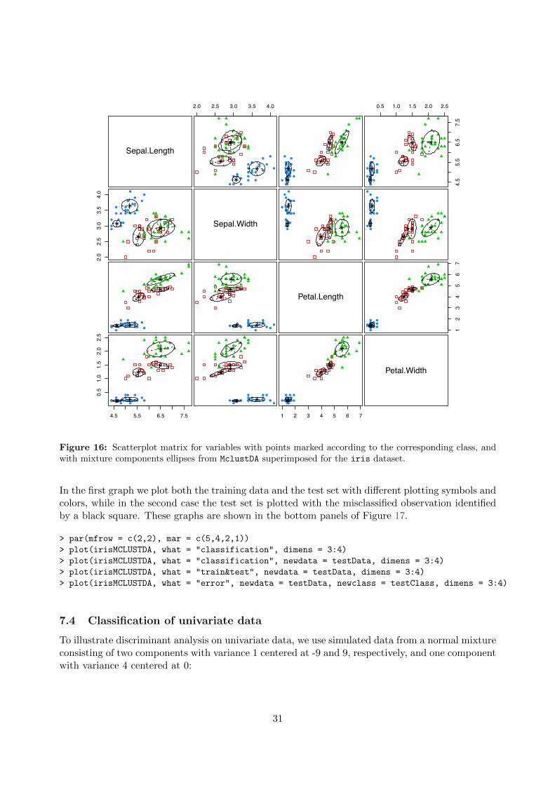
Sepal.Length

Sepal.Width

Sepal.Length

●

●

●

●●

●

●

●

●

●

●

●●●●

●

●

●

●

●

●

●

●●●

2.0 2.5 3.0 3.5 4.0

Petal.Length

Sepal.Length

●

●

●

●●

●

●

●

●

●

●

●●

●●

●

●

●

●

●

●

●

●●●

Petal.Width

Sepal.Length

●

●

●

●●

●

●

●

●

●

●

●●

●●

●

●

●

●

●

●

●

●●●

0.5 1.0 1.5 2.0 2.5

4.5

5.5

6.5

7.5

Sepal.Length

Sepal.W

idth ●

●

●

●

●

●

●

●●

●

●

●

● ● ●

●

●

●

●

●

●

●

●●●

2.0

2.5

3.0

3.5

4.0

Sepal.Width

Petal.Length

Sepal.W

idth ●

●

●

●

●

●

●

●●

●

●

●

●●●

●

●

●

●

●

●

●

●●●

Petal.Width

Sepal.W

idth ●

●

●

●

●

●

●

●●

●

●

●

● ●●

●

●

●

●

●

●

●

●●●

Sepal.Length

Petal.Length

●● ●●● ●●●●

●●

●

●●

●● ●●

●● ●●

●● ●

Sepal.Width

Petal.Length

●● ●●● ●●●●

●●

●

●●●

● ●●●● ●●

●●●

Petal.Length

Petal.Width

Petal.Length

●●●●●●●● ●

●●

●

●●

●●●●●●●●

●●●

12

34

56

7

Sepal.Length

Petal.W

idth

●● ●●

● ●●

●

●●

●● ●

●

●●●

● ●●●

●

●

● ●

4.5 5.5 6.5 7.5

0.5

1.0

1.5

2.0

2.5

Sepal.Width

Petal.W

idth

●● ●●

● ●●

●

●●

● ●●

●

●●●

● ●●●

●

●

●●

Petal.Length

Petal.W

idth

●●●●●●●

●

●●●● ●

●

●●●●●●

●●

●

●●

1 2 3 4 5 6 7

Petal.Width

Figure 16: Scatterplot matrix for variables with points marked according to the corresponding class, andwith mixture components ellipses from MclustDA superimposed for the iris dataset.

In the first graph we plot both the training data and the test set with different plotting symbols andcolors, while in the second case the test set is plotted with the misclassified observation identifiedby a black square. These graphs are shown in the bottom panels of Figure 17.

> par(mfrow = c(2,2), mar = c(5,4,2,1))> plot(irisMCLUSTDA, what = "classification", dimens = 3:4)> plot(irisMCLUSTDA, what = "classification", newdata = testData, dimens = 3:4)> plot(irisMCLUSTDA, what = "train&test", newdata = testData, dimens = 3:4)> plot(irisMCLUSTDA, what = "error", newdata = testData, newclass = testClass, dimens = 3:4)

7.4 Classification of univariate data

To illustrate discriminant analysis on univariate data, we use simulated data from a normal mixtureconsisting of two components with variance 1 centered at -9 and 9, respectively, and one componentwith variance 4 centered at 0:

31

1 2 3 4 5 6 7

0.5

1.0

1.5

2.0

2.5

Petal.Length

Petal.W

idth

●●●

●

●●

●

●

●

●

●● ●

●

● ●

●

●●●

●

●

●

●●

Training Data: known classification

1 2 3 4 5 6

0.5

1.0

1.5

2.0

2.5

Petal.LengthPetal.W

idth

●●

●

●

●

●

●

●

●●

●

●

●●●

●

●●

●

●

●

●

●

●●

Test Data: MclustDA classification

1 2 3 4 5 6 7

0.5

1.0

1.5

2.0

2.5

Petal.Length

Petal.W

idth

●●●

●

●●

●

●

●

●

●● ●

●

● ●

●

●●●

●

●

●

●●

●

●●

●

●

● ●

●

●●

●

●

●

●

●

●

●

● ●

●

●●

●●

●

●

●

●

●

●

●

●

●

●

●●

●

●

●

●

●

●

●

●

●

●

●

●

●

●

Training and Test Data

1 2 3 4 5 6

0.5

1.0

1.5

2.0

2.5

Petal.Length

Petal.W

idth

●

●

●

●

●

●

●

●

●

●

●

● ●●

●

●

●

●

●

●

● ●●

●

●

Test Error

Figure 17: Classification plots for a selected pair of variables with points marked according to the knownor estimated classification from MclustDA for the iris dataset.

> set.seed(0)> x <- c(rnorm(300, -9), rnorm(400, 0, sd = 2), rnorm(300, 9))> xClass <- rep(1:3, times = c(300,400,300))

We use the following simulated data as a test set:

> set.seed(1)> y <- c(rnorm(100, -9), rnorm(100, 0, sd = 2), rnorm(100, 9))> yClass <- rep(1:3, each = 100)

In both cases we set the seed of the random number generator so the exact example can be repro-duced.

In discriminant analysis with EDDA (Section 7.1) we assume that each component constitutesa separate group. We may use either leave-one-out crossvalidation or BIC for choosing between theonly two possible models for univariate data:

32

> cv1EMtrain(x,labels=xClass)

E V0.006 0.002

> bicEMtrain(x,labels=xClass)

E V-5786.7 -5607.2

The varying variance model V was selected as the optimal model for the training set under bothcriteria. The training and test errors for the data with this model are as follows:

> modV <- MclustDA(x, xClass, modelType = "EDDA", modelName = "V")> summary(modV, newdata = y, newclass = yClass)


EDDA model summary:

log.likelihood n df BIC-2776 1000 6 -5593.4

Classes n Model G1 300 V 12 400 V 13 300 V 1


PredictedClass 1 2 3

1 300 0 02 0 399 13 0 1 299


Test classification summary:

PredictedClass 1 2 3

1 100 0 02 0 100 03 0 0 100

Test error = 0

The classification and classification errors for the training data are shown in Figure 18 and havebeen obtained with the following code:

> par(mfrow = c(1,3), mar = c(4,4,2,1))> plot(modV)> plot(modV, what = "classification")> plot(modV, what = "error")

33

−10 −5 0 5 10

0.0

0.1

0.2

0.3

0.4

x

Density

−10 −5 0 5 10

x1

23

|| |||| | || |||| ||| || || | || || | ||| ||||| | ||| || ||||||| ||| || || || ||| | ||| || || |||||| | | ||||| | ||||| || || || || ||| || |||| || || || ||| ||| || |||||||| |||| | || || |||||| ||||||| | || || | |||| ||| || ||||| ||| || ||| || ||| ||| ||||| | ||| || | || ||||| ||| || ||| ||| | ||| | || || || || || | || || || | ||| | || ||| | || ||| || |||| || |||| || || || | | ||| | || ||| || ||| ||| || | || || || |||

|| |||| | || |||| ||| || || | || || | ||| ||||| | ||| || ||||||| ||| || || || ||| | ||| || || |||||| | | ||||| | ||||| || || || || ||| || |||| || || || ||| ||| || |||||||| |||| | || || |||||| ||||||| | || || | |||| ||| || ||||| ||| || ||| || ||| ||| ||||| | ||| || | || ||||| ||| || ||| ||| | ||| | || || || || || | || || || | ||| | || ||| | || ||| || |||| || |||| || || || | | ||| | || ||| || ||| ||| || | || || || |||

| || ||| | |||| || || || ||| |||| | |||| | ||||| ||||| | |||| || ||| | ||| | || ||| || | ||| || | || || | || || || || || || | || |||| ||| | |||| || || | || ||| || | | ||| ||| || || | || |||| | || ||| | |||||||| || | ||| || || | | | || || | || ||| ||| | || |||| | || ||| || | || | || ||| ||| | || | || |||| |||| || || ||| ||| || || || || || || | || ||| || | || || ||| ||| ||| |||| |||| || |||| |||| ||| |||||| ||| || ||| || || ||| || ||||| ||| | || | ||| || ||| | || | || || ||| || | || | || || || ||||| | ||||| | || || | || ||| | ||||| | || | || ||| || || | | |||| | ||| || | |

| || ||| | |||| || || || ||| |||| | |||| | ||||| ||||| | |||| || ||| | ||| | || ||| || | ||| || | || || | || || || || || || | || |||| ||| | |||| || || | || ||| || | | ||| ||| || || | || |||| | || ||| | |||||||| || | ||| || || | | | || || | || ||| ||| | || |||| | || ||| || | || | || ||| ||| | || | || |||| |||| || || ||| ||| || || || || || || | || ||| || | || || ||| ||| ||| |||| |||| || |||| |||| ||| |||||| ||| || ||| || || ||| || ||||| ||| | || | ||| || ||| | || | || || ||| || | || | || || || ||||| | ||||| | || || | || ||| | ||||| | || | || ||| || || | | |||| | ||| || | |

| ||| || | | |||| ||| | |||| || | ||| || ||| |||| || || || || || | || || || ||| ||| |||| | ||| |||| ||| ||| || | | |||| ||| | | || |||||| ||| ||| || || || || ||| ||||| ||| |||| || | ||| || ||| || | || | || | |||| || ||| |||| || || || ||| |||| ||| || ||| | |||||||||| ||||| ||||||| || |||| | || |||| | ||||| | || ||| || ||| || | || ||| | ||||| || || || || ||||| || ||| ||| | || | ||| ||| |||| | ||| ||| | ||||| || |||

| ||| || | | |||| ||| | |||| || | ||| || ||| |||| || || || || || | || || || ||| ||| |||| | ||| |||| ||| ||| || | | |||| ||| | | || |||||| ||| ||| || || || || ||| ||||| ||| |||| || | ||| || ||| || | || | || | |||| || ||| |||| || || || ||| |||| ||| || ||| | |||||||||| ||||| ||||||| || |||| | || |||| | ||||| | || ||| || ||| || | || ||| | ||||| || || || || ||||| || ||| ||| | || | ||| ||| |||| | ||| ||| | ||||| || |||Training Data: known classification

−10 −5 0 5 10

x

12

3

|| |||| | || |||| ||| || || | || || | ||| ||||| | ||| || ||||||| ||| || || || ||| | ||| || || |||||| | | ||||| | ||||| || || || || ||| || |||| || || || ||| ||| || |||||||| |||| | || || |||||| ||||||| | || || | |||| ||| || ||||| ||| || ||| || ||| ||| ||||| | ||| || | || ||||| ||| || ||| ||| | ||| | || || || || || | || || || | ||| | || ||| | || ||| || |||| || |||| || || || | | ||| | || ||| || ||| ||| || | || || || ||| | || ||| | |||| || || || ||| |||| | |||| | ||||| ||||| | |||| || ||| | ||| | || ||| || | ||| || | || || | || || || || || || | || |||| ||| | |||| || || | || ||| || | | ||| ||| || || | || |||| | || ||| | |||||||| || | ||| || || | | | || || | || ||| ||| | || |||| | || ||| || | || | || ||| ||| | || | || |||| |||| || || ||| ||| || || || || || || | || ||| || | || || ||| ||| ||| |||| |||| || |||| |||| ||| |||||| ||| || ||| || || ||| || ||||| ||| | || | ||| || ||| | || | || || ||| || | || | || || || ||||| | ||||| | || || | || ||| | ||||| | || | || ||| || || | | |||| | ||| || |

|

||| || | | |||| ||| | |||| || | ||| || ||| |||| || || || || || | || || || ||| ||| |||| | ||| |||| ||| ||| || | | |||| ||| | | || |||||| ||| ||| || || || || ||| ||||| ||| |||| || | ||| || ||| || | || | || | |||| || ||| |||| || || || ||| |||| ||| || ||| | |||||||||| ||||| ||||||| || |||| | || |||| | ||||| | || ||| || ||| || | || ||| | ||||| || || || || ||||| || ||| ||| | || | ||| ||| |||| | ||| ||| | ||||| || |||

|Train Error

Figure 18: LEFT: Densities for the univariate simulation data. There are two components with variance1 centered at -9 and 9, respectively, and one component with variance 4 centered at 0. CENTER: Trainingstep classification. RIGHT: Misclassified training observations.

To illustrate the discriminant analysis via the MclustDA methodology (see Section 7.2) weuse the same simulated univariate data as above but assume that observations are grouped bycomponent variance:

> xClass <- rep(c(1,2,1), times = c(300,400,300))> yClass <- rep(c(1,2,1), each = 100)

The training stage fits a two component equal-variance model to one group, and a one-componentmodel to the other:

> modMCLUSTDA <- MclustDA(x, xClass)> summary(modMCLUSTDA)




Classes n Model G1 600 E 22 400 X 1


PredictedClass 1 2

1 599 12 1 399


The classification error rates are the same as we obtained for discriminant analysis via EM withthe 3-class grouping.

34

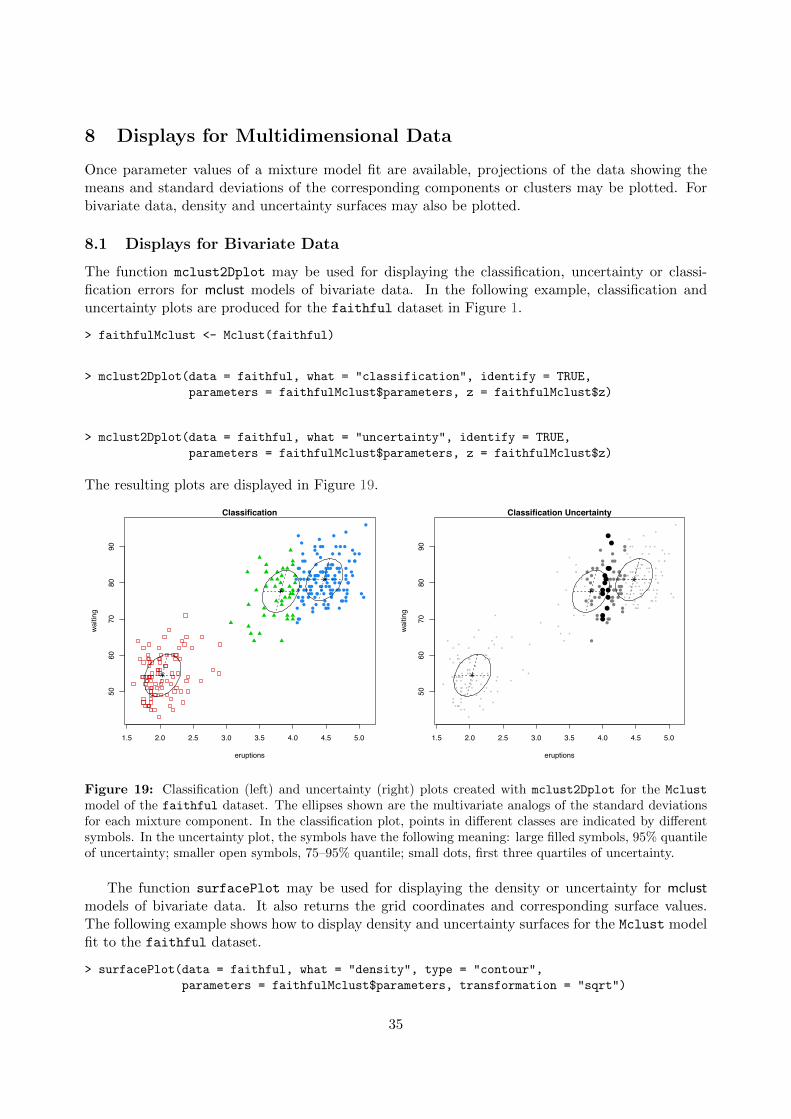
8 Displays for Multidimensional Data

Once parameter values of a mixture model fit are available, projections of the data showing themeans and standard deviations of the corresponding components or clusters may be plotted. Forbivariate data, density and uncertainty surfaces may also be plotted.

8.1 Displays for Bivariate Data

The function mclust2Dplot may be used for displaying the classification, uncertainty or classi-fication errors for mclust models of bivariate data. In the following example, classification anduncertainty plots are produced for the faithful dataset in Figure 1.

> faithfulMclust <- Mclust(faithful)

> mclust2Dplot(data = faithful, what = "classification", identify = TRUE,parameters = faithfulMclust$parameters, z = faithfulMclust$z)

> mclust2Dplot(data = faithful, what = "uncertainty", identify = TRUE,parameters = faithfulMclust$parameters, z = faithfulMclust$z)

The resulting plots are displayed in Figure 19.

1.5 2.0 2.5 3.0 3.5 4.0 4.5 5.0

5060

7080

90

eruptions

waiting

Classification

●

●

●

●

●●

●

●

●

●

●

●

●

●

●

●

●

●

●

●

●

●

●

●

●

●

●

● ●

●

●

●

●

●

●

●

●

●

●

●

●

●

●

●

●

●

●

●

●

●

●

●

●

●

●

●

●

●

●

●

●

●

●

●

●●

●●

●

●

●

●●

●

●

●

●

●

●

● ●

●●

●

●

●

●●

●

●

●

●

●●

●

●

●●

●

●

●

●

●

●

●

●● ●

●

●

●

●

●

●

●●

●

●

●

●

●

●

●●

●●

●

●

●

●

1.5 2.0 2.5 3.0 3.5 4.0 4.5 5.0

5060

7080

90

eruptions

waiting

Classification Uncertainty

●

●

●

●

●

●

●

●

●

●

●

●

●

●

●

●

●

●

●

●

●

●

●

●

●

●

●

●

●

●

●

●

●

●

●

●

●

●

●

●

●

●

●

●

●

●

●

●

●

●

●

●

●

●

●

●

●

●

●

●

●

●

●

●

●

●

●

●

●

●

●

●

●

●

●

●

●

●

●

●

●

●

●

●

●

●

●

●

●

●

●

●

●

●

●

●

●

●

●

●

●

●

●

●

●

●

●

●

●

●

●

●

●

●

●

●

●

●

●

●

●

●

●

●

●

●

●

●

●

●

●

●

●

●

●

●

●

●

●

●

●

●

●

●

●

●

●

●

●

●

●

●

●

●

●

●

●

●

●

●

●

●

●

●

●

●

●

●

●

●

●

●

●

●

●

●

●

●●

●

●

●

●

●

●

●

●

●

●

●

● ●

●

●

●

●

●

●

●

●

●

●

●

●

●

●●

●

●●

●

●

●

●●

●

●

●

●

●

●

●

●

●

●

●

●

●

●

●

●

●

●

●

●●

●

●

●

●●●

●

●●

● ●

●

●

●

●

●

●

●

●

●

●

●

●

●●

●●

●

●

●

●

●●

●

●●

Figure 19: Classification (left) and uncertainty (right) plots created with mclust2Dplot for the Mclustmodel of the faithful dataset. The ellipses shown are the multivariate analogs of the standard deviationsfor each mixture component. In the classification plot, points in different classes are indicated by differentsymbols. In the uncertainty plot, the symbols have the following meaning: large filled symbols, 95% quantileof uncertainty; smaller open symbols, 75–95% quantile; small dots, first three quartiles of uncertainty.

The function surfacePlot may be used for displaying the density or uncertainty for mclustmodels of bivariate data. It also returns the grid coordinates and corresponding surface values.The following example shows how to display density and uncertainty surfaces for the Mclust modelfit to the faithful dataset.

> surfacePlot(data = faithful, what = "density", type = "contour",parameters = faithfulMclust$parameters, transformation = "sqrt")

35

> surfacePlot(data = faithful, what = "uncertainty", type = "image",parameters = faithfulMclust$parameters, transformation = "log")

The resulting plots are displayed in Figure 20.

Density Uncertainty

eruptions

waiti

ng 0.02

0.02

0.04

0.04

0.04

0.06 0.06

0.08

0.08

0.1

0.1

0.12

0.12

0.14

0.14

0.16

0.16

0.18

0.18

0.2

1.5 2.0 2.5 3.0 3.5 4.0 4.5 5.0

5060

7080

90

2.0 2.5 3.0 3.5 4.0 4.5 5.0

5060

7080

90

eruptions

waiting

Figure 20: Density (left column) and uncertainty (right column) surfaces for the faithful dataset. Asquare root transformation was used for the density plot, which is plotted as a contour surface. A logarithmictransformation was used for the uncertainty plot, which is plotted as an image surface.

36

8.2 Displays for Higher Dimensional Data

8.2.1 Coordinate Projections

To plot coordinate projections in mclust use the function coordProj. The example we consider isa 3-group model for the iris dataset:

> irisBIC <- mclustBIC(iris[,-5])> irisSummary3 <- summary(irisBIC, data = iris[,-5], G = 3)

> coordProj(data = iris[,-5], dimens = c(2,4), what = "classification",parameters = irisSummary3$parameters, z = irisSummary3$z)

> coordProj(data = iris[,-5], dimens = c(2,4), what = "uncertainty",parameters = irisSummary3$parameters, z = irisSummary3$z)

> coordProj(data = iris[,-5], dimens = c(2,4), what = "errors",parameters = irisSummary3$parameters, z = irisSummary3$z, truth = iris[,5])

2.0 2.5 3.0 3.5 4.0

0.5

1.0

1.5

2.0

2.5

Sepal.Width

Petal.W

idth

●● ●● ●

●

●

●●

●

●●

●●

●

●●

● ●●

●

●

●

●

●●

●

●●●●

●

●

●● ● ●

●

● ●

●●

●

●

●

●

●● ●●

2.0 2.5 3.0 3.5 4.0

0.5

1.0

1.5

2.0

2.5

Sepal.Width

Petal.W

idth

●● ●● ●

●

●

●●

●

●●

●●

●

●●

● ●●

●

●

●

●

●●

●

●●●●

●

●

●● ● ●

●

● ●

●●

●

●

●

●

●● ●●

●

●

●

●

●

● ●

●

●

●

●

●

●

●

●

●

●

●

●

●

●

●

●

●

●

●●

●

●

●

●

●

●

●

●

●

●

●

●

●●

●

●

●

●

●

●

●

●

●

●

●

●

●

●

●

●

●

●

●

●

●

●

●●●

●

●

●

●

●

●

●

●

●

●

●

●

● ●

●

●

●

●

● ●●

● ● ●●●

●

●●

●

●

●

●

●

2.0 2.5 3.0 3.5 4.0

0.5

1.0

1.5

2.0

2.5

Sepal.Width

Petal.W

idth

●

●

●

●

●

●

●

●●

●

●

●

●

●

●

●

●

●

●

●

●

●●

●

●

●● ●

●

●

●

●

●

●

●

●

●

●●

●

●

●

●

●

●

●

●

●

●

●

Figure 21: A coordinate projection of the iris dataset created with coordProj. Plots show the 3-group model-based classification (top) with associated uncertainty (bottom, left) and classification errors(bottom,right).

These plots are displayed in Figure 21.

37

8.2.2 Random Projections

To plot random projections in mclust use the function randProj. Again we consider is a 3-groupmodel for the iris dataset:

> randProj(data = iris[,-5], seed = 43, what = "classification",parameters = irisSummary3$parameters, z = irisSummary3$z)



These plots are displayed in Figure 22.

−5.0 −4.5 −4.0 −3.5 −3.0 −2.5

−5.0

−4.5

−4.0

−3.5

−3.0

●

●

●

●

●

●

●

●

●

●

●

● ●

●

●

●

●

●

●

●

●

●

●

●

●

●

●

●●

●

●

●

●

●

●

●

●

●

●

●●

●●

●●

●

●

●

●

●

4.5 5.0 5.5 6.0 6.5 7.0

−4.0

−3.5

−3.0

−2.5

−2.0

−1.5

●

●

●●

●

●

●

●

●●

●●

●●

●

●

●

●

●

●

●

●

●●

●

●

●●

●●

●

●

● ●

●●

●

●

●

●●

●

●

●

●

●

●

●

●

●

−1.0 −0.8 −0.6 −0.4 −0.2 0.0 0.2 0.4

−6.5

−6.0

−5.5

−5.0

−4.5

−4.0

●

●

●

●

●

●

●

●

●

●

●

● ●

●

●

●

●

●

●

●

●

●

●

●

●

●●

●●

●

●

●

●

●

●

●

●

●

●

●●

●●

●●

●

●

●

●

●

Figure 22: Some random projections of the iris dataset created with randProj. Plots show the 3-groupclassification from model-based clustering with three different seeds.

38

8.3 Dimension reduction for model-based clustering and classification

New functionality has been added to mclust package for data projection on a dimension reducedsubspace [31]. This dimension reduction method allows the visualization of the clustering or clas-sification structure obtained from a Gaussian finite mixture model.

8.3.1 Clustering

Consider the following clustering scenario:

> MCLUST = Mclust(iris[,1:4])> MCLUST

'Mclust' model object:best model: ellipsoidal, equal shape (VEV) with 2 components

Once a mixture model has been fitted, we may want to look at a plot in a reduced subspace whichcapture most of the clustering structure contained in the data. The function MclustDR allows toestimate the basis of such subspace:

> DR = MclustDR(MCLUST)> summary(DR)

-----------------------------------------------------------------Dimension reduction for model-based clustering and classification-----------------------------------------------------------------

Mixture model type: Mclust

Estimated basis vectors:Dir1 Dir2 Dir3 Dir4

Sepal.Length 0.18224 -0.23497 0.53649 0.030665Sepal.Width 0.73764 0.16437 -0.36366 0.902191Petal.Length -0.60349 -0.27048 -0.49512 0.274447Petal.Width -0.24183 0.91903 0.57861 -0.331346

Dir1 Dir2 Dir3 Dir4Eigenvalues 0.85068 0.34586 0.064915 0.030269Cum. % 65.85600 92.63125 97.656678 100.000000

The directions which span the reduced subspace are defined as a set of linear combinations ofthe original features, ordered by importance as quantified by the associated eigenvalues. In theexample, the first two directions account for most of the clustering structure as shown in Figure 23.The graph is obtained with the following code:

> plot(DR, what = "evalues")

The main contribution to the first direction is from differences in cluster means, while for the seconddirection is from differences in cluster variances.

A scatterplot matrix of data projected onto the estimated subspace is shown in Figure 24 andit is obtained as follows:

> plot(DR)

Figure 25 contains examples of bivariate plots. The left graph is a bivariate contour plot ofmixture components densities:

39

●

●

●●

0.0

0.2

0.4

0.6

0.8

MclustDR directions

Eige

nval

ues

1 2 3 4

● EigenvaluesMeans contrib.Vars contrib.

Figure 23: Plot of eigenvalues from MclustDR applied to a clustering model for the iris dataset.

> plot(DR, what = "contour")

while the graph on the right is a scatterplot with uncertainty boundaries:

> plot(DR, what = "boundaries")

where the uncertainty is shown using a greyscale with darker regions indicating higher uncertainty.Both plot projects the data onto the first two directions, i.e., using the default argument dimens= c(1,2). Setting this argument to any other pair of values produces a projection along differentdirections.

Marginal distributions along selected directions can be obtained as follows:

> plot(DR, what = "density", dimens = 1)> plot(DR, what = "density", dimens = 2)

and they are shown in Figure 26.Many other graphs can be obtained by specifying the argument what. The interested reader

may consult help(plot.MclustDR) for a comprehensive list and examples.

8.3.2 Classification

The method illustrated for clustering can also be applied to a classification scenario, except thatnow we must take into account that known classes can be made of one or more mixture components.For example, consider the banknote dataset contained in mclust:

> data(banknote)> MCLUSTDA = MclustDA(data = banknote[,-1], class = banknote$Status)> summary(MCLUSTDA)

------------------------------------------------Gaussian finite mixture model for classification

40

●

●

●

●●

●

●

●

●

●

●

●

●

●

●

●

●

●

●

●

●

●

●

●

●●

●

●●●

●

●

●

●

●

●

●

●

●

●

●

●

●

●

●●

●

●

●●

−2 −1 0 1 2

−0.4

−0.2

0.0

0.2

0.4

0.6

Dir1

Dir2

Figure 24: Scatterplot of clustering structure from MclustDR for the iris dataset.

------------------------------------------------



Classes n Model Gcounterfeit 100 EEE 3genuine 100 XXX 1


PredictedClass counterfeit genuinecounterfeit 100 0genuine 0 100

Training error = 0

> DR = MclustDR(MCLUSTDA)> summary(DR)

-----------------------------------------------------------------Dimension reduction for model-based clustering and classification-----------------------------------------------------------------

Mixture model type: MclustDA

41

−2 −1 0 1 2

−0.4

−0.2

0.0

0.2

0.4

0.6

Dir1

Dir2

●●

●

● ●

●

●

●

●

●

●

●

●

●

●

●●

●

●

●

●

●

●

●

●●

●

●●●●

●

●

●

●

●

●●

●

●

●

●

●

●

●●

●

●

●●

−2 −1 0 1 2

−0.4

−0.2

0.0

0.2

0.4

0.6

Dir1Dir2

●●

●

● ●

●

●

●

●

●

●

●

●

●

●

●●

●

●

●

●

●

●

●

●●

●

●●●●

●

●

●

●

●

●●

●

●

●

●

●

●

●●

●

●

●●

Figure 25: Contour plot of mixture densities (left) and uncertainty boundaries (right) from MclustDR forthe iris dataset.

0.0

0.2

0.4

0.6

0.8

1.0

1.2

Dir1

Density

−2 −1 0 1 2

Dir1

1

2

01

23

4

Dir2

Density

−0.4 −0.2 0.0 0.2 0.4 0.6

Dir2

1

2

Figure 26: Marginal mixture densities for the first two directions from MclustDR for the iris dataset.

Estimated basis vectors:Dir1 Dir2 Dir3 Dir4 Dir5 Dir6

Length -0.094293 -0.32902 -0.0043289 -0.385202 0.703088 0.551233Left -0.318248 -0.40252 -0.8638528 0.700590 0.492784 -0.036375Right 0.223543 -0.12154 0.2911526 -0.587057 0.018105 -0.811847Bottom 0.621442 0.47022 -0.0486602 -0.010436 0.111424 0.093691Top 0.553684 0.28743 -0.2984504 -0.116710 -0.496313 0.153537Diagonal -0.383536 0.64127 -0.2784408 -0.049267 -0.061325 -0.058068

Dir1 Dir2 Dir3 Dir4 Dir5 Dir6Eigenvalues 0.87532 0.60038 0.17223 0.066972 0.02501 1.8745e-03Cum. % 50.25411 84.72339 94.61147 98.456517 99.89238 1.0000e+02

42

A pairs plot of the data projected along the first three directions is obtained with code:

> plot(DR, what = "pairs", dim = 1:3)

Dir1

−2.0 −1.5 −1.0 −0.5 0.0 0.5 1.0

●

●

●

●

●

●

●

●

●

●

●

●

●●

●

●

●

●

●

●

●

●●

●●

●●

●

●●

●●

● ● ●

●●

●

●●

●

● ●

●

−2−1

01

2

●

●

●

●

●

●

●

●

●

●

●

●

●●

●

●

●

●

●

●

●

●●

●●

●●

●

●●

●●

● ●●

●●

●

● ●

●

● ●

●

−2.0

−1.5

−1.0

−0.5

0.0

0.5

1.0

●●

●

●

●

●●

●

●

●

●●

●●

●

●●

●

● ●

● ●●

●

●●

●●

●●●●

●

●

●

●

●

●

●●●

●

●

●

Dir2

●●

●

●

●

●●

●

●

●

●●

●●

●

●●

●

●●

●●●

●

● ●

●●

●● ●●

●

●

●

●

●

●

●●●

●

●

●

−2 −1 0 1 2

●

●●

●

●

●

●

●

●

●

●

●

●

●●

●

●

●

●

●

● ●

●

●

●

●

●

●

●

●

●

●

●

●

●

●

●

●

●

●

●

●

●

●

●

●●

●

●

●

●

●

●

●

●

●

●

● ●

●

●

●

●

●

●●

●

●

●

●

●

●

●

●

●

●

●

●

●

●

●

●

●

●

●

●

●

●

−0.5 0.0 0.5−0.5

0.0

0.5

Dir3

Figure 27: Pairs plot for the first three dimensions from MclustDR for the banknote dataset.

A bivariate contour plot of mixture components densities for each class and the classificationboundaries are given by:

> plot(DR, what = "contour")> plot(DR, what = "boundaries")

9 Combining Gaussian Mixture Components for Clustering

In traditional model-based clustering, each cluster corresponds to a single mixture component.However, it may be desirable in some situations to model a single cluster using several mixturecomponents. The function clustCombi provides a means for obtaining models with clusters repre-sented by multiple mixture components.

Consider the following simulated dataset from a bivariate Gaussian mixture distribution:

> data(Baudry_etal_2010_JCGS_examples)> MCLUST <- Mclust(ex4.1)> MCLUST

43

−2 −1 0 1 2

−2.0

−1.5

−1.0

−0.5

0.0

0.5

1.0

Dir1

Dir2

●●

●

●

●

●●

●

●

●

●●

●●

●

●●

●

● ●

● ●●●

●●

●●

●●●●

●

●●

●

●

●

●●●

●

●

●

−2 −1 0 1 2

−2.0

−1.5

−1.0

−0.5

0.0

0.5

1.0

Dir1Dir2

●●

●

●

●

●●

●

●

●

●●

●●

●

●●

●

● ●

● ●●●

●●

●●

●●●●

●

●●

●

●

●

●●●

●

●

●

Figure 28: Contour plot of mixture densities for each class (left) and classification boundaries (right) fromMclustDR for the banknote dataset.

'Mclust' model object:best model: ellipsoidal, equal volume and shape (EEV) with 6 components

The function clustCombi combines the mixture components hierarchically according to an entropycriterion, following the methodology in [3]. The solutions with numbers of classes between thenumber of components selected by BIC and one are returned:

> CLUSTCOMBI <- clustCombi(ex4.1, MCLUST)> CLUSTCOMBI

EM/BIC Solution---------------

Number of components: 6Model name: EEV

Component num.1:proportion: 0.12mean: 7.92 -0.02

Component num.2:proportion: 0.20mean: 8.07 4.98



Component num.5:proportion: 0.22mean: -0.02 0.06

Component num.6:proportion: 0.08

44

mean: 8.10 0.17

Combining steps---------------

Step | Classes combined at this step | Classes labels after this step-------|-------------------------------|-------------------------------

0 | --- | 1 2 3 4 5 61 | 3 & 4 | 1 2 3 5 62 | 1 & 6 | 1 2 3 53 | 3 & 5 | 1 2 34 | 1 & 2 | 1 35 | 1 & 3 | 1

Classification for K classes: output$classification[[K]]Combining matrix (K classes -> (K-1) classes): output$combiM[[K]]

The output shows the the components proportions and means of the fitted Gaussian mixture model,followed by the informations about the combining steps.

−2 0 2 4 6 8 10

−20

24

6

X1

X2

●● ●

●● ●●●●

●

●●

●● ●

●● ●●

●●●●

● ● ●

● ●●●●

●●

●

●●●

●

●●

●●

● ●

●

●●

●●

●●

●●●

●●●●●

●●●●

●●

●●●●

●●

●●●●●

●●

●

BIC solution ( 6 clusters)

−2 0 2 4 6 8 10

−20

24

6

X1

X2

●● ●

●● ●●●●

●

●●

●● ●

●● ●●

●●●●

● ● ●

● ●●●●

●●

●

●●●

●

●●

●●

● ●

●

●●

●●

●●

●●●

●●●●●

●●●●

●●

●●●●

●●

●●●●●

●●

●

Combined solution with 5 clusters

−2 0 2 4 6 8 10

−20

24

6

X1

X2

●

●

●

●●

●

●

●●

●

●

●

●

●

●

●

●

●

●

●

●

●●● ●

● ●●

●

●●●

●●●●

● ● ●

● ●

●●

●

●

●

●

●●●

●

●

●

●●

●

●●

●

●

●

●

● ●

●●●

●●

●●

●

●●

●●●

●

●

●

●

●●●

●

●

●●

●

●

●

●●

●

●

●●

●

●

●

●●

●

●●●

●●

●●●●

●●

●●●

●


−2 0 2 4 6 8 10

−20

24

6

X1

X2

●

●

●

●●

●

●

●●

●

●

●

●

●

●

●

●

●

●

●

●

●●● ●

● ●●

●

●●●

●●●●

● ● ●

● ●

●●

●

●

●

●

●●●

●

●

●

●●

●

●●

●

●

●

●

● ●

●●●

●●

●●

●

●●

●●●

●

●

●

●

●●●

●

●

●●

●

●

●

●●

●

●

●●

●

●

●

●●

●

●●●

●●

●●●●

●●

●●●

●


−2 0 2 4 6 8 10

−20

24

6

X1

X2

●

●

●

●●●

●

●

●

●

●

●

●

●

●

●

●

●

●●

●

●

●

●

●●

●

●

●

●

●

●

●

●

●

●

●

●

●

●

●

●

●

●

●● ●

●

●

●

●

●

●

●

●

●

● ●

●

●

●

●

●

●●

●

●

●●●

● ● ●

●

● ●

●

●

●

●

●

●

●

●

●

●

●

●

●

●●

●

●●

●

●

●●

●

●

●

●

●

●

●

●

●

●

●

●

●

●

●

●

●

●

●

●

●

●

●

●

●

●

●

●

● ●

●

●

●

●

●

●

●

●

●

●

●

●

●●

●

●

●●

●

●

●

●

●

●●

●

●

●

●

●

●

●

●

●●

●

●

●

●

●

●

●

●

●

●

●

●

●

●

●

●

●

●

●

●

●

●

●

●

●

●●●

●

●

●

●

●

●

●

●

●

●

●

●●

●

●

●

●●

●

●●

●

●

●

●

●

●

●

●●

●

●

●

●

●

●

●

●

●

●●●

●

●●●

●

●

●


−2 0 2 4 6 8 10

−20

24

6

X1

X2

●

●

●●

●

●

●

● ●

●●●

●

● ●

●

●●

●●

●

●

●

●●

●

●

●

●

●

●

●

●

●

●

●

●

●

●

●

●

●

●

●

●

●

●

●

●●●●

●

●

●

●

●

●

● ●

●

●

●

●

● ●

●

●●

●●

●

●

●

●●

●

●●

●●

●

●

●

●

●

●

●

●

●

●

●

●

●

●

●

●

●●

●

●

●●●

●

●

●

●

●

●

●

●

●

●

●

●

●

●

●

●●

●

●

●

●

●

●

●

●

●

●

●

●

●

●

●

●

●

●

●

●

●●

●

●

● ●

●

● ●

●

●●

●

●

●

● ●

●

●

●

●

●

●

●

●

●

● ●

●

●

●

●

●

●

●

●

●

●

●

●

●

●

●

●

●

●

●

●●

●●

●

●●

●

●

●

● ●

●

●

●

●●

●

●

● ●

● ●

●

● ●

●

●

●

●

●

●

●

●

●

●

●

●

●

●

●

●

●

●

●

●

●

●●●

●

●

●●

●

●

● ●

●●

●●

●●

●

●

●

●

●

●

●●

●

●

●

●

●

●

●

●

●

●

●●

●●

●●

●

●

●

●

●

●

●

●

●

●

●

●

●

●

●

●

●●

●●●

●

●

●

●

●

●●

●

●

●

●

●

●

●

●

●

●

●

●

●

●●

●●●

●

●

●

● ●

●

●

● ●

●●

●

●

●

●

●

●

●

●

●

●

●

●

●

● ●●

●

●

●

●

●

●

●●

●

●

●

●

●

●

● ●●

●

●

●

●

●

●

●

●

● ●

●

●

●

●

●

●

●

●

●

●

●

●

●

●

●

●

●

●

●

●

●

●

●

●

●

●

●

●

●

●

●

●

●

●

●

●

●●

●

●●

●

●

●

●

●

●

●

●

●

●

●

●

●

●●

●

●

●

●

●

●

●

●

●

●

●

●●

●

●

●

●

●

●

●

●

●

● ●

●

●

●

●

●

●

●

●

●

●

●

●

●

●

●

●

●

●●

●

●

●

●●

●

●

●

●

●

●

●

●

●

●

●●

●

●

●

●

●

●

●

●

●

●

●

●

●● ●

●

●

●

●

●

●

●

●●

●

●

●●

●

●

●

●

●

●●

● ●

●

●

●

● ●●

●

●

●

●

●

●

●

●

●

●

●

●●

●

●

●

●

●

●

●

●

●

●●

●

●

●

●

●

●

●

●

●

●

●

●

●

●

●

●

●

●

●

●

●

●

●

●

●

●

●

●

●

●

●

●

●

●

●

●

●

●

●

●

●


Figure 29: Solutions from combining mixture components for the ex4.1 dataset.

The plot method displays the hierarchy of combined solutions and then some “entropy plots”which may help a user to select the optimal number of clusters:

> plot(CLUSTCOMBI, ex4.1)

45

The graphs are shown in Figure 29 and 30, with the entropy plots which suggests a four-clusterssolution.

● ● ●●

●

●

1 2 3 4 5 6

020

4060

8010

012

0

Number of clusters

Entro

py

● ●●

●

●

1 2 3 4 5

020

4060

80Number of clusters

Diff

eren

ce in

ent

ropy

Entropy plot

● ● ●●

●

●

0 500 1000 1500

020

4060

8010

012

0

Cumul. count of merged obs.

Entro

py

● ●●

●●

1 2 3 4 5

0.0

0.1

0.2

0.3

Number of clusters

Nor

mal

ized

diffe

renc

e in

ent

ropy

Normalized entropy plot

Figure 30: Entropy plots for combining mixture components for the ex4.1 dataset.

46

10 Simulation from Mixture Densities

Given the parameters for a mixture model, data can be simulated from that model for evaluationand verification. The function sim allows simulation from mixture models generated by mclustfunctions. Besides the model, sim allows a seed as input for reproducibility. As an example,below we simulate two different datasets of the same size as the faithful dataset from the modelproduced by Mclust for the faithful dataset:

> faithfulMclust <- Mclust(faithful)> sim0 <- sim( modelName = faithfulMclust$modelName,

parameters = faithfulMclust$parameters,n = nrow(faithful), seed = 0)

> sim1 <- sim(modelName = faithfulMclust$modelName,parameters = faithfulMclust$parameters,n = nrow(faithful), seed = 1)

The results can be plotted as follows:

> xlim <- range(c(faithful[,1],sim0[,2],sim1[,2]))> ylim <- range(c(faithful[,2],sim0[,3],sim1[,3]))> mclust2Dplot(data=faithful, parameters = faithfulMclust$parameters,

classification = faithfulMclust$classification, xlim = xlim, ylim = ylim)> mclust2Dplot(data=sim0[,-1], parameters = faithfulMclust$parameters,

classification = sim0[,1], xlim = xlim, ylim = ylim)> mclust2Dplot(data=sim1[,-1], parameters = faithfulMclust$parameters,

classification = sim1[,1], xlim = xlim, ylim = ylim)

The plots are shown in Figure 31. Note that sim produces a dataset in which the first column isthe classification.

11 Extensions

11.1 Large Datasets

Mclust and mclustBIC include a provision for using a subsample of the data in the hierarchicalclustering phase before applying EM to the full data set, in order to extend the method to largerdatasets. Some other methods for handling such cases are discussed in [34, 19]. The followingexample uses a random sample of size 100 in the initial hierarchical clustering phase of EMclustapplied to the iris data:

> nrow(iris)

[1] 150

> S <- sample(1:nrow(iris), size = 100)> Mclust(iris[,-5], initialization = list(subset = S))

'Mclust' model object:best model: ellipsoidal, equal shape (VEV) with 3 components

For very large data sets, the capabilities of mclust can be easily used for classification. First,a discriminant analysis with the methodology implemented in MclustDA can be performed on asubset of the data. Then the remaining data points can then be classified (in reasonable sizedblocks) using the predict method as described in section 7.

47

2 3 4 5

4050

6070

8090

eruptions

waiting

●

●

●

●

●●

●

●

●

●

●

●

●

●

●

●

●

●

●

●

●

●

●

●

●

●

●

● ●

●

●

●

●

●

●

●

●

●

●

●

●

●

●

●

●

●

●

●

●

●

●

●

●

●

●

●

●

●

●

●

●

●

●

●

●●

●●

●

●

●

●●

●

●

●

●

●

●

● ●

●●

●

●

●

●●

●

●

●

●

●●

●

●

●●

●

●

●

●

●

●

●

●● ●

●

●

●

●

●

●

●●

●

●

●

●

●

●

●●

●●

●

●

●

●

2 3 4 5

4050

6070

8090

1

2

●

●

●

●

●

●

●

●

●

●

●

●

●

●

●

●

●

●

●

●

●

●

●●

●

●●

●

●

●

●

●

●●

●

●

●●

●

●

●

●

●

●

●

●

●●

●

●

●

●

●

●

●

●

●

●

●

●

● ●●

●

●

●

●

●

●

●

●●

●

●

●

●

● ●

●

●

●●

●

●

●

●

●●

●●

●

●

●

●

●●

●

●

●

● ●

●

●

●

●

●

●

●

●

●

●

●

●

●

●

●

●

●●

●

●

●

●

●●

2 3 4 5

4050

6070

8090

1

2

●

●

●

●

●●●

●

●

●

●

●

●

●

●

●

●

●

●

●

●

●●

●●

●●

●

●

●

●

●

●

●

●

●

●

●

●

●

●

●

●●

●

●

●

●

●

● ●

●

●

●

●

●

●

●●● ●

●

●

●

●

●

●

●

●●

●

●

●

●●

●

●

●

●

●

●

●

●

●

●

●

●

●

●●

●

●

●

●

●

●

●

●

●

●

●

●

●

●

● ●

●

●

●

●

●

●

●

●●

●●

●

●

●

●

●

●

●

●

●

Figure 31: Data simulated from a model of the faithful dataset. The top hand figure is the faithfuldataset, and the bottom figures are datasets of the same size simulated from the Mclust model for thefaithful dataset. The ellipse defined by the covariance matrices of the model is shown on all of the plots.

11.2 High-Dimensional Data

Models in which the orientation is allowed to vary between clusters (EEV, VEV, EVV, VVV), have O(d2)parameters per cluster, where d is the dimension of the data. For this reason, mclust may not workwell or may otherwise be inefficient for these models when applied to high-dimensional data. It maystill be possible to analyze such data with mclust by restriction to models with fewer parameters(e.g. spherical or diagonal models), or else by applying a dimension-reduction technique such asprincipal components.

Some of the more parsimonious models (e.g. spherical, diagonal, or fixed covariance) can beapplied to datasets in which the number of observations is smaller than the data dimension.

11.3 Missing Data

At present, mclust has no direct provision for handling missing values in data. However, a functionimputeData has been added to the mclust package for creating datasets with missing data imputa-tions using the mix package. Here we illustrate the use of the imputeData to fill in missing values

48

in the continuous portion of the stlouis dataset provided with the mix package (we remove thefirst 3 categorical variables, since mclust is intended for continuous variables).

> library(mix)> data(stlouis)> dim(stlouis)

[1] 69 7

> head(stlouis)

G D1 D2 R1 V1 R2 V24001 1 NA 1 110 NA NA 1504004 1 1 2 118 165 NA 1304005 1 2 NA 116 145 114 1254006 1 NA NA NA NA 126 NA4008 1 1 NA 118 140 118 1234009 1 NA NA NA 120 105 138

> stlimp <- imputeData( stlouis[,-(1:3)])

Steps of EM:1...2...3...4...5...6...7...8...9...10...11...12...13...14...15...16...17...18...19...20...21...22...23...24...25...Steps of Data Augmentation:1...2...3...4...5...6...7...8...9...10...11...12...13...14...15...16...17...18...19...20...21...22...23...24...25...26...27...28...29...30...31...32...33...34...35...36...37...38...39...40...41...42...43...44...45...46...47...48...49...50...51...52...53...54...55...56...57...58...59...60...61...62...63...64...65...66...67...68...69...70...71...72...73...74...75...76...77...78...79...80...81...82...83...84...85...86...87...88...89...90...91...92...93...94...95...96...97...98...99...100...

Note that the values obtained for the missing entries will vary depending on the random numberseed set in function imputeData, chosen randomly by default. It is usually desirable to combinemultiple imputations in analyses involving missing data. See [23] for details and references onmultiple imputation.

Another function imputePairs has been added to the mclust package for visualizing missingdata imputations:

> imputePairs(stlouis[,-(1:3)], stlimp)

A pairs plot showing the imputed values is displayed in Figure 32.

12 Function Summary

12.1 Hierarchical Clustering

hc Merge sequences for model-based hierarchical clustering.hclass Classifications corresponding to hc results.

12.2 Parameterized Gaussian Mixture Models

em EM algorithm (starting with E-step).me EM algorithm (starting with M-step).

me.weighted EM algorithm with weights (starting with M-step)estep E-step of the EM algorithm.mstep M-step of the EM algorithm.mvn One-component fit.

12.3 Density Computation for Parameterized Gaussian Mixtures

cdens Component density (without mixing proportions).dens Mixture density.

49

R1

50 100 150 200

●

●●

●●

●

●

●

●

●

●

●

●

●

●●

●

●

●

●

●

●

●●

●

●●●

●

●

●

●

●

●●

●

●

●

●●●

●

●

●

●

●

●

●

●

●

●

●

●

●

●

●

●

●

●

●

●●

●

●

●

●

●

●

●

●

●●

●●

●

●

●

●

●

●

●

●

●

●●

●

●

●

●

●

●

●●

●

●●●

●

●

●

●

●

●●

●

●

●

●●●

●

●

●

●

●

●

●

●

●

●

●

●

●

●

●

●

●

●

●

●●

●

●

●

●

●

●

●

60 80 100 140 180

6080

100

120

140

●

●●

●●

●

●

●

●

●

●

●

●

●

●●

●

●

●

●

●

●

●●

●

●● ●

●

●

●

●

●

●●

●

●

●

●●●

●

●

●

●

●

●

●

●

●

●

●

●

●

●

●

●

●

●

●

●●

●

●

●

●

●

●

●

50100

150

200

● ●

●

●

●

●●

●

●

●●

●

●

●

●

●

●

●

●

●

●

●

●

●

●●

●●

●●

●

●

●

●

●

●

●

●

●

●

●

●

●

●

●

●

●

●

●

●

●●

●

●

●

●

●

●

●

●

●

●

●

●

●

●

●

●

● V1

●●

●

●

●

●●

●

●

●●

●

●

●

●

●

●

●

●

●

●

●

●

●

●●

●●

●●

●

●

●

●

●

●

●

●

●

●

●

●

●

●

●

●

●

●

●

●

●●

●

●

●

●

●

●

●

●

●

●

●

●

●

●

●

●

●

●●

●

●

●

●●

●

●

●●

●

●

●

●

●

●

●

●

●

●

●

●

●

●●

●●

●●

●

●

●

●

●

●

●

●

●

●

●

●

●

●

●

●

●

●

●

●

●●

●

●

●

●

●

●

●

●

●

●

●

●

●

●

●

●

●

●

●

●

●

●

●

●

●

●

●

●

●

●

●

●

●

●

●

●

●

●

●

●

●

●

●

●

●

●

●

●●

●

●

●

●

●●

●

●

●

●

●● ●

●

●

●

●

●

●

●

●●

●

●

●

●

● ●

●

●

●

●

●

●

●

●

●

●

●

●

●

●

●

●

●

●

●

●

●

●

●

●

●

●

●

●

●

●

●

●

●

●

●

●

●

●

●

●●

●

●

●

●

●●

●

●

●

●

●● ●

●

●

●

●

●

●

●

●●

●

●

●

●

● ●

●

●

●

●

●

●

●

●

●

R2

8090

100

120

140

●

●

●

●

●

●

●

●

●

●

●

●

●

●

●

●

●

●

●

●

●

●

●

●

●

●

●

●

●

●

●●

●

●

●

●

●●

●

●

●

●

●● ●

●

●

●

●

●

●

●

●●

●

●

●

●

●●

●

●

●

●

●

●

●

●

●

60 80 100 120 140

6080

120

160

200

●

●●

●

●

●

●

●●

●

●

●

●

●●

●

●

●

●

●

●

●

●

●

●

●

●

●

●

●

●

●

●

●

●

●

●●

●

●

●

●

●

●

●

●●

●

●

●

●

●

●

●

●

●

●

●

●●

●

●

●

●

●

●

●

●

●

●

●●

●

●

●

●

●●

●

●

●

●

●●

●

●

●

●

●

●

●

●

●

●

●

●

●

●

●

●

●

●

●

●

●

●●

●

●

●

●

●

●

●

●●

●

●

●

●

●

●

●

●

●

●

●

●●

●

●

●

●

●

●

●

●

●

80 90 100 110 120 130 140

●

●●

●

●

●

●

●●

●

●

●

●

●●

●

●

●

●

●

●

●

●

●

●

●

●

●

●

●

●

●

●

●

●

●

●●

●

●

●

●

●

●

●

● ●

●

●

●

●

●

●

●

●

●

●

●

●●

●

●

●

●

●

●

●

●

●

V2

Figure 32: Example of missing data imputations obtained via the mix package for the continuous variablesin the stlouis dataset. The closed black circles correspond to nonmissing data, while the open red circlescorrespond to imputed missing values.

50

12.4 Model-based Clustering

mclustBIC BIC computation; clusters and models through summary.Mclust Model-based clustering.

clustCombi Combining Gaussian mixture components for clustering.

12.5 Model-based Density Estimation

densityMclust Density estimation via Mclust.

12.6 Discriminant Analysis

Class Densities as Mixture Components:

cv1EMtrain Training via leave-one-out crossvalidation.bicEMtrain Training via BIC.

estep E-step of the EM algorithm.mstep M-step of the EM algorithm.

MclustDA Model-based classification using modelType = "EDDA".

Parameterized Gaussian Mixture for Class Densities (MclustDA):

MclustDA Model-based classification using default argument modelType = "MclustDA".predict.MclustDA MclustDA classification.

cv.MclustDA k-fold cross-validation for MclustDA.

12.7 Bayesian Regularization

priorControl specify a prior distribution.defaultPrior default prior distribution.

12.8 Support for Modeling and Classification

mclust.options set or retrieve mclust options.mclustModel specify an mclust model.

mclustModelNames description for an mclust model.mclustVariance template for (co)variance specification of an mclust model.

emControl specify parameters affecting EM.map Convert conditional probabilities to a classification.

unmap Convert a classification to indicator variables.bic BIC for parameterized Gaussian mixture models.sim Simulate data from a parameterized Gaussian mixture model.

mapClass Mapping between two classifications.classError Classification error.

adjustedRandIndex Adjusted Rand Index.sigma2decomp Convert mixture covariances to decomposition form.decomp2sigma Convert decomposition form to mixture covariances.nVarParams Number of variance parameters.imputeData Missing data imputation using the mix package.

51

12.9 Plotting Functions

Univariate Data

mclust1Dplot Classification, uncertainty, density and/or classification errors.plot.densityMclust Plot method associated with the densityMclust function.

Bivariate Data

mclust2Dplot Classification, uncertainty, and/or classification errors.surfacePlot Contour, image, or perspective plot of either density or uncertainty.

More than Two Dimensions

Classification, uncertainty, and/or classification errors:

coordProj Coordinate projections.randProj Random projections.MclustDR Dimension reduction for model-based clustering and classification.

12.9.1 Other Plotting Functions

clPairs Pairs plot showing classification.imputePairs Pairs plot to show missing data imputations.uncerPlot Relative uncertainty of misclassified observations.

plot.Mclust Plots associated with Mclust results.plot.mclustBIC BIC plot associated with mclustBIC results.plot.mclustDA Plots associated with mclustDA results.plot.mclustDR Plots associated with mclustDR results.

plot.clustCombi Plots associated with clustCombi results.

52

A Appendix

A.1 Clustering Models

mclust usually assumes a normal or Gaussian mixture model

n�

i=1

G�

k=1

τk φk(xi | µk,Σk),

where where x represents the data, G is the number of components, τk is the probabilty that anobservation belongs to the kth component (τk ≥ 0;

�Gk=1 τk = 1) , and

φk(x | µk,Σk) = (2π)−p2 |Σk|

− 12 exp

�−1

2(xi − µk)

TΣ−1k (xi − µk)

�. (1)

The exception is for model-based hierarchical clustering, for which the model used is the classifica-tion likelihood with a parameterized normal distribution assumed for each class:

n�

i=1

φ�i(xi | µ�i ,Σ�i),

where the �i are labels indicating a unique classification of each observation: �i = k if xi belongsto the kth component.

The components or clusters in both these models are ellipsoidal, centered at the means µk. Thecovariances Σk determine their other geometric features. Each covariance matrix is parameterizedby eigenvalue decomposition in the form

Σk = λkDkAkDTk ,

where Dk is the orthogonal matrix of eigenvectors, Ak is a diagonal matrix whose elements areproportional to the eigenvalues of Σk, and λk is a scalar (Banfield and Raftery 1993). The orien-tation of the principal components of Σk is determined by Dk, while Ak determines the shape ofthe density contours; λk specifies the volume of the corresponding ellipsoid, which is proportionalto λd

k |Ak|, where d is the data dimension. Characteristics (orientation, volume and shape) of dis-tributions are usually estimated from the data, and can be allowed to vary between clusters, orconstrained to be the same for all clusters [27, 2, 8]. This parameterization includes but is notrestricted to well-known variance models that are associated with various criterion for hierarchicalclustering, such as equal-volume spherical variance (Σk = λI) for the sum of squares criterion [33],constant variance [20], and unconstrained variance [30].

In one dimension, there are just two models: E for equal variance and V for varying variance.In more than one dimension, the model identifiers code geometric characteristics of the model.For example, EVI denotes a model in which the volumes of all clusters are equal (E), the shapesof the clusters may vary (V), and the orientation is the identity (I). Clusters in this model havediagonal covariances with orientation parallel to the coordinate axes. Parameters associated withcharacteristics designated by E or V are determined from the data. Table 1 shows the variousmultivariate model options currently available in mclust for hierarchical clustering (denoted HC)and EM. These are a subset of the parameterizations discussed in [8], which gives details of the EMalgorithm for maximum likelihood estimation for these models.

53

A.2 Modeling Noise and Outliers

mclust uses a mixture model which has a single term representing noise as a first order Poissonprocess to handle noisy data:

n�

i=1

�τ0V

+G�

k=1

τkφk(xi | θk)

�, (2)

in which V is the hypervolume of the data region, and τk ≥ 0;�G

k=0 τk = 1. This model has beenused successfully in a number of applications [2, 9, 6, 7].

The basic model-based clustering method needs to be modified when the data contains noise.First, a good initial noise estimate must be obtained. Some possible methods for denoising include aVoronoı method [1], a nearest-neighbor method [5], and robust covariance estimation [32]. The func-tion NNclean in the contributed R package prabclus is an implementation of the nearest-neighbormethod. The function cov.nnve in the contributed R package covRobust is an implementation ofrobust covariance estimation. Next, hierarchical clustering is applied to the denoised data. Finally,EM based on the Gaussian model with the added noise term (2) is applied to the entire data set,with the data removed in the denoising process as the initial noise estimate.

A.3 Model Selection via BIC

Several measures have been proposed for choosing the clustering model (parameterization andnumber of clusters); see, e.g., Chapter 6 of [26]. We use the Bayesian Information Criterion (BIC)approximation to the Bayes factor [29], which adds a penalty to the loglikelihood based on thenumber of parameters, and has performed well in a number of applications (e.g. [11, 13]). The BIChas the form

BIC ≡ 2 loglikM(x, θ∗k)− (# params)M log(n), (3)

where loglikM(x, θ∗k) is the maximized loglikelihood for the model and data, (# params)M is thenumber of independent parameters to be estimated in the model M, and n is the number ofobservations in the data.

A.4 Adding a Prior to the Model

By default, mclust does not use a prior for modeling. However, users can optionally specify aconjugate prior of the type described in this section. For univariate data, we use a normal prior onthe mean (conditional on the variance):

µ | σ2 ∼ N (µP ,σ2/κP)

∝�σ2

�− 12 exp

�−

κP

2σ2(µ− µP)

2� (4)

and an inverse gamma prior on the variance:

σ2 ∼ inverseGamma(νP/2, ς2P/2)

∝�σ2

�− νP+22 exp

�−

ς2P2σ2

�.

(5)

For multivariate data, we use a normal prior on the mean (conditional on the covariance matrix):

µ | Σ ∼ N (µP ,Σ/κP)

∝ |Σ|−12 exp

�−κP

2trace

�(µ− µP)

T Σ−1 (µ− µP)��

,(6)

54

and an inverse Wishart prior on the covariance matrix:

Σ ∼ inverseWishart(νP ,ΛP)

∝ |Σ|−νP+d+1

2 exp

�−1

2trace

�Σ−1Λ−1

P

��.

(7)

The hyperparameters µP , κP , and νP are called the mean, shrinkage and degrees of freedom, re-spectively. Parameters ς2P (a scalar) and ΛP (a matrix) are the scale of the prior distribution inthe univariate and multivariate cases, respectively. These priors are called conjugate priors for thenormal distribution because the posterior can be expressed as the product of a normal distributionand an inverse gamma or Wishart distribution. With the prior, a modified version of the BIC,in which the MLE is replaced by the MAP, is used to choose the number of clusters. Details onmodel-based clustering with a prior can be found in [17].

Functions priorControl and defaultPrior are provided in mclust for specifying a prior. Whencalled with defaults, the following choices are made for the prior hyperparameters:

µP = the mean of the data.

κP = .01

The posterior meannkyk + κPµP

κP + nkcan be viewed as adding κP observations with value µP to

each group in the data. The value we used was determined by experimentation; values closeto and bigger than 1 caused large perturbations in the modeling in cases where there were nomissing BIC values without the prior. The value .01 resulted in BIC curves that appeared tobe smooth extensions of their counterparts without the prior.

νP = d+ 2Analogously to the univariate case, the marginal prior distribution of µ is a t distributioncentered at µP with νP − d + 1 degrees of freedom. The mean of this distribution is µP

provided that νP > d, and it has a finite covariance matrix provided νP > d + 1 (see, e. g.Schafer 1997). We chose the smallest integer value for the degrees of freedom that gives afinite covariance matrix.

ς2P =sum(diag(var(data)))/d

G2/d (for univariate models, and multivariate spherical or diagonal mod-els)The average of the diagonal elements of the empirical covariance matrix of the data dividedby the square of the number of components to the 1/d power. This is roughly equivalent topartitioning the range of the data into G intervals of fairly equal size.

ΛP =var(data)

G2/d (for multivariate ellipsoidal models)The empirical covariance matrix of the data divided by the square of the number of compo-nents to the 1/d power.

55

References

[1] D. Allard and C. Fraley. Nonparametric maximum likelihood estimation of features in spatialpoint processes using Voronoı tessellation. Journal of the American Statistical Association,92:1485–1493, 1997.

[2] J. D. Banfield and A. E. Raftery. Model-based Gaussian and non-Gaussian clustering. Bio-metrics, 49:803–821, 1993.

[3] J.-P. Baudry, A. E. Raftery, G. Celeux, K. Lo and R. Gottardo. Combining mixture componentsfor clustering. Journal of Computational and Graphical Statistics, 19(2):332-353, 2010.

[4] H. Bensmail, and G. Celeux. Regularized Gaussian Discriminant Analysis Through EigenvalueDecomposition. Journal of the American Statistical Association, 91:1743–1748, 1996.

[5] S. D. Byers and A. E. Raftery. Nearest neighbor clutter removal for estimating features inspatial point processes. Journal of the American Statistical Association, 93:577–584, 1998.

[6] J. G. Campbell, C. Fraley, F. Murtagh, and A. E. Raftery. Linear flaw detection in woventextiles using model-based clustering. Pattern Recognition Letters, 18:1539–1548, 1997.

[7] J. G. Campbell, C. Fraley, D. Stanford, F. Murtagh, and A. E. Raftery. Model-based methodsfor real-time textile fault detection. International Journal of Imaging Systems and Technology,10:339–346, 1999.

[8] G. Celeux and G. Govaert. Gaussian parsimonious clustering models. Pattern Recognition,28:781–793, 1995.

[9] A. Dasgupta and A. E. Raftery. Detecting features in spatial point processes with clutter viamodel-based clustering. Journal of the American Statistical Association, 93:294–302, 1998.

[10] C. Fraley. Algorithms for model-based Gaussian hierarchical clustering. SIAM Journal onScientific Computing, 20:270–281, 1998.

[11] C. Fraley and A. E. Raftery. How many clusters? Which clustering method? - Answers viamodel-based cluster analysis. The Computer Journal, 41:578–588, 1998.

[12] C. Fraley and A. E. Raftery. MCLUST: Software for model-based cluster analysis. Journal ofClassification, 16:297–306, 1999.

[13] C. Fraley and A. E. Raftery. Model-based clustering, discriminant analysis and density esti-mation. Journal of the American Statistical Association, 97:611–631, 2002.

[14] C. Fraley and A. E. Raftery. Enhanced software for model-based clustering, density estimation,and discriminant analysis: MCLUST. Journal of Classification, 20:263–286, 2003.

[15] C. Fraley and A. E. Raftery. Model-based microarray image analysis. R News, 6:60–63, 2006.

[16] C. Fraley and A. E. Raftery. Some applications of model-based clustering in chemistry. RNews, 6:17–23, 2006.

[17] C. Fraley and A. E. Raftery. Bayesian regularization for normal mixture estimation and model-based clustering. Journal of Classification, 24:155–181, 2007.

56

[18] C. Fraley and A. E. Raftery. Model-based methods of classification: using the mclust softwarein chemometrics. Journal of Statistical Software, 18(6), January 2007.

[19] C. Fraley, A. E. Raftery, and R. Wehrens. Incremental model-based clustering for large datasetswith small clusters. Journal of Computational and Graphical Statistics, 14:1–18, 2005.

[20] H. P. Friedman and J. Rubin. On some invariant criteria for grouping data. Journal of theAmerican Statistical Association, 62:1159–1178, 1967.

[21] G. H. Golub and C. F. Van Loan. Matrix Computations. Johns Hopkins, 3rd edition, 1996.

[22] L. Hubert and P. Arabie. Comparing partitions. Journal of Classification, 2:193–218, 1985.

[23] R. J. A. Little and D. B. Rubin. Statistical Analysis with Missing Data. Wiley, 2nd edition,2002.

[24] C. Loader. Local Regression and Likelihood. Springer, New York, 1999.

[25] K. V. Mardia, J. T. Kent, and J. M. Bibby. Multivariate Analysis. Academic Press, 1979.

[26] G. J. McLachlan and D. Peel. Finite Mixture Models. Wiley, 2000.

[27] F. Murtagh and A. E. Raftery. Fitting straight lines to point patterns. Pattern Recognition,17:479–483, 1984.

[28] J. L. Schafer. Analysis of Incomplete Multivariate Data by Simulation. Chapman and Hall,1997.

[29] G. Schwarz. Estimating the dimension of a model. The Annals of Statistics, 6:461–464, 1978.

[30] A. J. Scott and M. J. Symons. Clustering methods based on likelihood ratio criteria. Biomet-rics, 27:387–397, 1971.

[31] L. Scrucca. Dimension reduction for model-based clustering. Statistics and Computing,20(4):471–484, 2010.

[32] N. Wang and A. E. Raftery. Nearest neighbor variance estimation (NNVE): Robust covarianceestimation via nearest neighbor cleaning (with discussion). Journal of the American StatisticalAssociation, 97:994–1019, 2002.

[33] J. H. Ward. Hierarchical groupings to optimize an objective function. Journal of the AmericanStatistical Association, 58:234–244, 1963.

[34] R. Wehrens, L. Buydens, C. Fraley, and A. Raftery. Model-based clustering for image segmen-tation and large datasets via sampling. Journal of Classification, 21:231–253, 2004.

57

mclust Version 4 for R: Normal Mixture Modeling for …...mclust Version 4 for R: Normal Mixture...

Documents

Transcript of mclust Version 4 for R: Normal Mixture Modeling for …...mclust Version 4 for R: Normal Mixture...