McClelland and Vallabha 2/26/2007 Page - Stanford...

McClelland and Vallabha 2/26/2007

Connectionist Models of Development:

Mechanistic Dynamical Models with Emergent Dynamical Properties

James L. McClelland and Gautam Vallabha

The symbolic paradigm of cognitive modeling, championed by Minsky and Papert,

Newell and Simon, and other pioneers of the 1950’s and 1960’s, remains very much alive and

well today. Yet an alternative paradigm, first championed in the 1950’s by Rosenblatt, in which

cognitive processes are viewed as emergent functions of a complex stochastic dynamical system,

has continued to have adherents. A cooling of interest in such approaches in the 1960’s did not

deter Grossberg (1976, 1978a) or James Anderson (1973), and the approach emerged again full

force in the 1980’s. Thereafter, many others begun to explore the implications of this paradigm

for development (Elman et al., 1996; McClelland, 1989; Plunkett and Marchman, 1993; Schulz,

Mareschal & Schmidt, 1994). A parallel and closely related movement, emerging from the

physical sciences, also began to gain adherents during the same decade (Schöner & Kelso, 1988)

and began to attract the interest of developmental psychologists in the early 1990s (Thelen &

Smith, 1994).

The present chapter represents our attempt to underscore the common ground between

connectionist and dynamical systems approaches. Central to both is the emergent nature of

system-level behavior and changes to such behavior through development.

1. Mechanistic and Emergent Dynamics


We first make a key distinction between mechanistic and emergent dynamics, which

parallels one made by Schöner and Kelso (1988) in their seminal article. We consider a

mechanism to be a set of rules or equations that stipulate certain microscopic behaviors in a

system. For example, the Hodgkin-Huxley equations stipulate certain relations between the

membrane potentials and neurotransmitter concentrations; these relations are considered to be

causal (and hence mechanistic) because of the underlying biology and chemistry. When the

stipulations are in the form of differential equations, the resulting system behavior is its

"mechanistic dynamics". Such behavior is usually unsurprising since it has been stipulated to be

just so. When several mechanistic subsystems interact, however, there is the possibility of

surprising behavior. We term such behavior "emergent", and it is typically at a different level of

description than the mechanistic dynamics. For example, lateral inhibition may lead to sharper

tuning curves and heightened contrast, but the terminology of "tuning curve" and "contrast" is a

step removed from the mechanistic level of membrane potentials and neurotransmitters. Such

emergent properties may have their own (non-stipulated) temporal evolutions, and we term such

evolutions the "emergent dynamics".

The above terminology allows a crisp characterization of connectionism and dynamical

systems theory. Both approaches assume that (a) mechanistic dynamics are best described by

differential equations that are rooted in biology, and that (b) psychological phenomena such as

categorization and selection reflect the emergent dynamics of the system. The key theoretical

issue is not just to describe the emergent dynamics, but also to explain how it arises from the

underlying mechanistic dynamics. This last point is crucial, since it distinguishes both

approaches from others in which the focus is on a descriptive characterization of the emergent

dynamics.


A further characteristic of connectionist systems is a graded notion of emergent

dynamics. Before elaborating on this, it is helpful to consider the four parts of a generic

connectionist system. These are schematically depicted in Figure 1, and consist of (1) a set of

differential equations stipulating how the inputs to units are related to their activations, (2) a set

of differential equations stipulating how the connection weights between the units are to be

updated, (3) the environment of the system, which provides the input stimulation, and (4) the

mismatch between the system's behavior and the target behavior, aka. the error. The "units" are

akin to pools of neurons and the activations are akin to the population activity of these neurons.

Consequently, the activations are influenced by the current weights and the environment; the

weight changes are influenced by the activations and the mismatch; and the mismatch itself is

influenced by the environment and the activations (which constitute the ongoing "behavior" of

the system).

[Insert Figure 1 about here]

There are several things to note about the generic system. First, its "mechanistic

dynamics" are simply those that result from the differential equations. These mechanistic

dynamics can give rise to emergent dynamics. Examples include the tuning curves and contrast

that emerge from lateral inhibition, or the spatial organization that emerges from competitive

topographic maps (e.g., Kohonen, 1982). Second, the weights can change over a variety of

timescales but the activations are assumed to only change over a fast time scale. This difference

in timescale for the mechanistic dynamics leads to a difference in timescale for the emergent

dynamics. Thus, there can be short-term emergent dynamics (in the range of milliseconds to

seconds) that coexist with long-term emergent dynamics (in the range of minutes to years). The

former are used to model activation processes that are assumed to be complete in the range of a


second, such as the process involved in settling on a perceptual interpretation of a visual input,

like a line drawing or a word. The latter are assumed to operate over a developmental timescale,

and may therefore also be termed developmental dynamics.

Since the focus of many connectionist models has been on change over developmental

time, their emphasis tends to fall on the time-evolution of the connections. Within multi-layer

connectionist networks, this time evolution can have complex dynamical properties, undergoing

both accelerations and decelerations, even though the weight-change mechanism itself does not

undergo any change. We shall consider such issues in detail later, but for now the essential point

is this: Connectionist systems are dynamical systems, and like other dynamical systems they can

have complex emergent properties which themselves may be described by dynamical variables

(rates of change with respect to time) and dynamical structures (attractors, transitions, and

instabilities).

Now we can elaborate the earlier observation that connectionist systems have a graded

notion of emergent dynamics. On a short time scale, connection weights can be treated as fixed,

contributing (along with the architecture of the system and the mechanistic dynamics of the

activations) to the emergent time-course and outcome of a single act of information processing

and/or behavior, such as reaching to one of two locations. Over a longer time scale (measured in

months or years), changes in the connection weights lead to changes in the short-term emergent

dynamics and may make possible new kinds of behavior (i.e., an 20-month old infant may

remember and reach differently than a 10-month old). Consequently, "emergence" is not sharply

demarcated in time or scale -- it occurs gradually and concurrently at different time scales, with

long-term emergence shaping the short-term emergent behaviors and vice versa. Both the short-

and long-term behaviors exhibit properties congruent with those postulated by Dynamical


Systems Theory (DST), as articulated by Schöner and Kelso (1988, Schöner, this volume). What

connectionism adds over and above this is an explanation of how the different scales of

emergence are related.

2. Examples of Activation and Weight-change Dynamics

The system in Figure 1 is very abstract, so it is helpful to consider a few concrete cases.

One example of activation dynamics is the cascade model (McClelland, 1979), which describes

the time-evolution of activation across the units in a linear, feed-forward network.

( )iii anetdta −=Δ λ

∑=s sisi awnet

(1) (2)

Here, ai is the activation of the ith unit, neti is its net input, and wis is the weight of the

connection from unit s to unit i. Essentially, the activation of a unit tends to change slowly

toward its instantaneous net input. While some units receive direct stimulation from the outside

world, most units receive their input from other units, and thus, what determines their activation

is the matrix of values of their incoming connection weights. The model showed that changes in

the parameters of Equation 1 (the mechanistic dynamics) modulated the overall system behavior

(the short-term emergent dynamics). For example, changes in the rate constants at two different

layers of the cascaded, feedforward network had additive effects on reaction time at the system

level.

More complex equations are often used in other models (e.g., Grossberg, 1978b):

( ) ( ) ( )ramaIaMEdta iiii −−−+−=Δ γβα (3) Grossberg’s formulation separates the excitatory input E and the inhibitory input I (where

E ≥ 0 and I ≤ 0) and lets each drive the activation up or down by an amount proportional to the

distance from the current activation to the maximum M or minimum m. Also operating is a


restoring force driving the activation of units back toward rest r; each force has its own strength

parameter (α, β, and γ). A similar function was used in the interactive activation model

(McClelland and Rumelhart, 1981). Analogous to Equation 2, E and I are essentially the sum of

the excitatory inputs (mediated by excitatory connections) and inhibitory inputs (mediated by

inhibitory connections). In his pioneering work in the 1970’s Grossberg examined in detail the

conditions under which these mechanistic dynamics gave rise to stable emergent behaviors such

as attractors and various other important emergent structures (Grossberg, 1978b).

In the above two examples, short-term emergent behavior arises from the mechanistic

dynamics of the activation updates. However, weight update dynamics may also lead to

emergent behavior. For example, Linsker (1986) suggested that the update of the connection

weight from a sending neuron s to a receiving neuron r might obey a Hebbian-type learning rule:

( )( ) rsssrrrs waadtdw βε −Θ−Θ−= (4) Here ar and as are the activations of the receiving and sending units, β is a constant

regulating a tendency for weights to decay toward 0, ε is the learning rate, and Θr and Θs are

critical values that can have their own mechanistic dynamics. Linsker (1986) showed that

Equation 4 can lead to receptive fields with surprisingly complex structure, such as center-

surround and orientation selectivity. In other words, the weight-update dynamics stipulated in

Equation 4 regulate the long-term emergent behavior of the system.

As with activation functions, many variations have been proposed for connectionist

learning rules. What is crucial for the moment is that the time-evolution of the connections in the

system -- the parameters which determine the emergent dynamics and outcome of the short-term

processing -- are themselves defined in terms of differential equations. The results of these

connection dynamics are emergent cognitive structures such as feature detectors, phonetic and


other types of categories, and behavioral abilities, as well as emergent dynamical trajectories of

change in such properties.

3. Simplified mechanisms

The discussion thus far has sidestepped a crucial issue. Equations 1-4, while relatively

close to the neurophysiology, are still highly abstract. For example, Equation 4 assumes that the

receiving and sending units' activity is exactly synchronized, though recent work suggests a

complex role for asynchrony (Roberts & Bell, 2002). So at what level should the mechanistic

dynamics be stipulated?

The pragmatic answer is that it depends on the research problem at hand. In some cases,

the focus is on the short-term emergent dynamics so the mechanics of the weight-change get

simplified. In a Hopfield net (Hopfield, 1982), for example, the weights may be calculated

beforehand from the training ensemble and thus there are no weight-change dynamics at all.

Likewise, in the interactive activation model (McClelland & Rumelhart, 1981) or the model of

the Stroop effect (Cohen, Dunbar & McClelland, 1990), the weights are directly stipulated by the

modeler so as to yield particular activation dynamics. The converse – where activation dynamics

are simplified so as to focus on the long-term emergent dynamics -- can also happen. In the

Kohonen (1982) map, the activation dynamics are simplified so that the input unit with the

maximum input is stipulated to be the winner and assigned an activation of 1.0. This allows the

modeler to focus on the weight change mechanisms and the developmental emergence of the

topographic map. (Kohonen, 1993, examines how this simplification may be reconciled with

more realistic activation dynamics.) Likewise, Carpenter and Grossberg's (1987) ART1 model,


and Rumelhart and Zipser (1985) use binary inputs and simplified activation in order to focus on

the unsupervised competitive learning.

Simplification of the activation dynamics sometimes goes hand in hand with a simplified

weight-change dynamics. This is the case when a network is trained using backpropagation,

which updates each weight in proportion to its influence on the overall error (Rumelhart, Hinton

and Williams, 1986). Backpropagation as numerically implemented is biologically implausible,

and the mechanics of the weight update may be much more complex (e.g., the LEABRA

algorithm; O'Reilly and Munakata, 2000). However, backpropagation is a useful simplification

that allows one to study how network architecture, statistical structure of the input, and

experience history interact to produce particular patterns of emergent long-term behavior.

It is important to note that many connectionist models simplify the activation dynamics in

ways that may mislead those unfamiliar with the framework about the underlying theory. For

example, in most connectionist models of past-tense verb inflection or single word reading, an

input pattern is propagated forward through one or more layers of connection weights to an

output layer. Furthermore, learning and performance variability is usually introduced through

initial randomization of the weights and the schedule of training but not in the propagation of

activity during a single trial. Such models may lead to the misconception that connectionist

theories advocate non-dynamic and non-stochastic processing. However, this is not the case. The

final output of the network represents an asymptotic (i.e., stable or settled) state that would be

achieved in an identical cascaded feedforward network or even a recurrent network (see Plaut et

al, 1996, for an explicit comparison of one-pass feedforward and recurrent versions of a network

for single-word reading). Likewise, while intrinsic variability (such as due to neural noise) is

often left out of specific models for simplicity, it is assumed to always to be at work in


processing (McClelland, 1991, 1993). Similar simplifications are often made in simple recurrent

networks (Elman, 1990), which can be viewed as chunking time into relatively large-scale,

discrete units, and setting the state for the next discrete unit based on the state of the one before.

While the networks look discrete, this is to be understood as an approximation that increases the

computational feasibility of a simulation, since allowing a network to settle over many time steps

multiplicatively scales the time it takes to run the simulation. For example, if there are 10 time

steps per simulated time unit, the simulation can take 10 times as much memory and take 10

times as long to run (Williams & Zipser, 1995).

Another simplification often found in connectionist systems concerns the input

representation, specifically, whether it is localist or distributed. In a localist input representation,

only one input unit is active at a given time, whereas in a distributed representation several units

may concurrently active. Distributed representations are more plausible from both a

computational and biological point of view: they allow many more stimuli to be represented (an

N-unit distributed representation can potentially represent 2N patterns, whereas a localist

representation can only represent N patterns), they can capture the similarity structure between

the input stimuli (due to the overlap between the distributed representations), and they are more

in line with what is known about neural representations (e.g., Haxby et al., 2001). Hence, a

localist representation is often a simplification of an underlying distributed representation. Such

a simplification has some theoretical support. For example, Kawamoto and Anderson (1985)

examined the competition between distributed representations in an attractor network, and found

that the dynamics of the competition mimicked those between two units. That is, in certain cases

the interaction between distributed patterns (between different spatial “modes”) may be recast as

an interaction between localist units.


In summary, then, connectionist systems are dynamical systems that can have both short-

and long-term emergent behavior. These emergent behaviors may themselves be described by

dynamical variables such as attractors and transitions, and are therefore similar in spirit to the

models postulated in Dynamical Systems Theory. In what follows, the points above will be

elaborated through the presentation of a series of models.

We begin with the recent model of activation dynamics proposed by Usher and

McClelland (2001), showing how a simple architecture can give rise to interesting emergent

dynamical properties (including attractors and path-dependence) which we will treat collectively

as the emergent response dynamics of the connectionist system. We will then consider a more

complex model proposed by Vallabha and McClelland (in press) which embeds the Usher-

McClelland activation dynamics within a network with simple weight-change dynamics, thereby

allowing it to learn in response to experience and exhibit interesting developmental dynamics in

the domain of acquisition of phonological distinctions. Further emergent dynamic properties will

be explored within this context. Finally we will consider a model by Rogers and McClelland

(2004) which addresses the time evolution of conceptual category representations. This model

simplifies both the activation and weight-change dynamics (as in the past-tense verb inflection

and reading models mentioned above) to address the gradual evolution of semantic category

representations over the first ten years of life. Once again, simple learning rules give rise to

complex emergent dynamical properties, now seen at a developmental time scale. Overall we

hope to bring out how these models instantiate many of the properties of the dynamical models

that have been proposed by many of the other contributors to this volume.


4. Short-term Emergent Dynamics in Perceptual Classification

We begin with Usher and McClelland's (2001) model of the time-course and accuracy of

responding in speeded perceptual classification tasks. The goal of this model was to provide an

account of classification responses, including time-accuracy tradeoffs and reaction-time

distributions, as a function primarily of the difficulty of the classification. Its architecture is very

similar to that used in PDP models of reading (McClelland and Rumelhart, 1981) and speech

perception (McClelland & Elman, 1986; McClelland, 1991), and incorporates the basic

principles of graded, interactive and stochastic processing. At its simplest level, the model

consists of a layer of units, in which each unit corresponds to one response (Figure 2a). Each unit

i receives excitatory activity ρi from an input layer that represents the external evidence or

"support" for that particular response. In addition, each unit has an excitatory connection to itself

and inhibitory connections to all other units in that layer. The key premise of the model is that

each unit takes up the external evidence in a cumulative and noisy manner while competing with

the other units. It is important to keep in mind that this is an abstract description of a system of

mutual constraints that does not impose a specific division between perceptual and motor

processing. For example, each "unit" may be instantiated as a spatially dispersed pattern of

neural activity that encompasses both perceptual and motor systems.


The dynamics of this system are governed by a set of stochastic nonlinear differential

equations:

dtdtffxdx iji jiiii ξβαλρ +⋅−+−= ∑ ≠][ (5)

where ρi is the external input to unit i, xi is the unit's instantaneous net input (its

"current"), fi is the instantaneous output (its "firing rate"; fj is likewise the output of unit j), α is


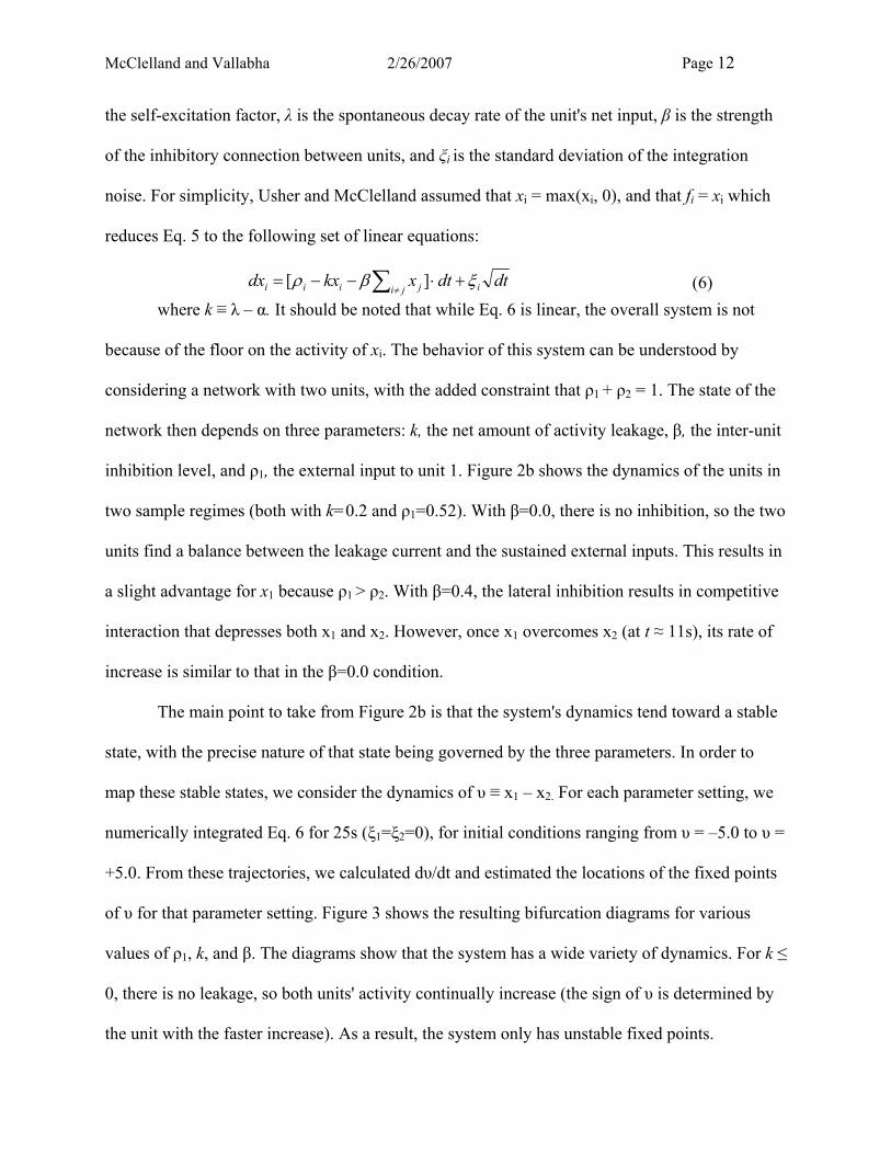
the self-excitation factor, λ is the spontaneous decay rate of the unit's net input, β is the strength

of the inhibitory connection between units, and ξi is the standard deviation of the integration

noise. For simplicity, Usher and McClelland assumed that xi = max(xi, 0), and that fi = xi which

reduces Eq. 5 to the following set of linear equations:

dtdtxkxdx iji jiii ξβρ +⋅−−= ∑ ≠][ (6)

where k ≡ λ – α. It should be noted that while Eq. 6 is linear, the overall system is not

because of the floor on the activity of xi. The behavior of this system can be understood by

considering a network with two units, with the added constraint that ρ1 + ρ2 = 1. The state of the

network then depends on three parameters: k, the net amount of activity leakage, β, the inter-unit

inhibition level, and ρ1, the external input to unit 1. Figure 2b shows the dynamics of the units in

two sample regimes (both with k=0.2 and ρ1=0.52). With β=0.0, there is no inhibition, so the two

units find a balance between the leakage current and the sustained external inputs. This results in

a slight advantage for x1 because ρ1 > ρ2. With β=0.4, the lateral inhibition results in competitive

interaction that depresses both x1 and x2. However, once x1 overcomes x2 (at t ≈ 11s), its rate of

increase is similar to that in the β=0.0 condition.

The main point to take from Figure 2b is that the system's dynamics tend toward a stable

state, with the precise nature of that state being governed by the three parameters. In order to

map these stable states, we consider the dynamics of υ ≡ x1 – x2. For each parameter setting, we

numerically integrated Eq. 6 for 25s (ξ1=ξ2=0), for initial conditions ranging from υ = –5.0 to υ =

+5.0. From these trajectories, we calculated dυ/dt and estimated the locations of the fixed points

of υ for that parameter setting. Figure 3 shows the resulting bifurcation diagrams for various

values of ρ1, k, and β. The diagrams show that the system has a wide variety of dynamics. For k ≤

0, there is no leakage, so both units' activity continually increase (the sign of υ is determined by

the unit with the faster increase). As a result, the system only has unstable fixed points.


Once k > 0, however, the net leakage dominates the external inputs and restricts the

overall levels of υ. Furthermore, the final state of the system is sensitive to the initial condition

υ0. If inhibition is weak, the input ρ1 allows one unit to quickly overwhelm the other, even if the

other unit has a slight initial advantage (see, for example, k = 0.2, β ≤ 0.2). If the inhibition is

strong, however, the initial state υ0 allows a unit to establish a decisive early advantage. For

example, let k=0.2, β ≥ 0.4, ρ1 = 0.6, and υ0 = –2. Unit 1 has a slight input advantage, but the υ0

allows unit 2 to suppress unit 1’s activity and win the competition. On the other hand, if the υ0 ≥

0 (or some critical value υ*) then obviously Unit 1 will win the competition. Thus, there is

bistability in the dynamics. If the inhibition is even greater (e.g., β=0.6), the early advantage is

established more rapidly, i.e., an input ρ1 is more likely to be overcome by an initial bias υ0.

Consequently, the bistable regime becomes wider as the inhibition β increases. The bistability

also implies that the system is capable of hysteresis. Say ρ1 is initially 0.0, so that system settles

at υ–. If ρ1 is then gradually ramped up, the system will stay at υ– until the end of the bistable

regime, at which point it will snap to υ+. If ρ1 is then gradually decreased, the system will stay at

υ+ during the bistable regime, indicating path dependence in the system dynamics.

A key point to keep in mind here is that the U-M model was not designed to produce the

dynamics in Figure 3. Its purpose was to account for ensemble statistics of categorization

performance using the principles of interactive, stochastic and graded processing (Usher &

McClelland, 2001), and the dynamical properties fell out as one consequence of these principles.

Furthermore, if Eq (2) is augmented with an additional depression term (so that a unit is less able

to compete if it has recently been active), its dynamics become remarkably similar to those of an

explicitly dynamical model of categorization (Tuller et al., 1994; Ditzinger et al., 1997). This

kinship suggests that the PDP approach (as instantiated in the U-M model) and the dynamical


approach (as instantiated through the dynamic field or synergetic approaches, see Schöner, this

volume) are in fact closely related approaches to the characterization of response dynamics.


5. Developmental Emergent Dynamics I: Perceptual Learning

There are two broad ways in which developmental dynamics have been explored within

the connectionist approach, one based on supervised error-driven training and the other based on

unsupervised Hebbian learning. The power of the former method is that it can re-represent the

input in sophisticated ways to match the task at hand (for example, a network may assign finer-

grain representations to salient inputs and coarser-grain ones to unimportant or rare inputs).

However, in many cases it is not plausible to assume that outcome information is consistently

available, and unsupervised learning based on Hebbian learning can provide insight into such

problems (Rumelhart & Zipser, 1985; Petrov et al., 2005). In addition, there is substantial

evidence for the biological plausibility of Hebbian learning (Ahissar, 1998; Syka, 2002). Finally,

Hebbian learning with bidirectional weights typically results in symmetric connections that

facilitate interactive attractor dynamics (Grossberg, 1988).

The relation between Hebbian learning and developmental dynamics was explored in a

model proposed by Vallabha and McClelland (in press). The motive for the model was to

provide an account for the initial acquisition of speech categories in infancy, the establishment of

such categories as attractors, the role of such attractors in creating difficulty in learning new

speech categories in adulthood, and how acquisition is affected by different training conditions.

Here we present a simplified version of this model that focuses on the emergence of a

"perceptual magnet effect" (Kuhl, 1991) as a result of perceptual experience. The effect is


marked by a decrease in discriminability between adjacent stimuli as they get closer to the

category prototype, and it is developmental in that it only shows up for sound categories that are

distinguished in the native language (Iverson et al., 2003). We will focus on how exposure to

native like sound structure results in the formation of perceptual categories, and how these in

turn affect discrimination, producing a perceptual magnet effect. Below we describe how the

Vallabha-McClelland model addresses this issue.

The model consists of two layers of units: L1 and L2 (Figure 4), with 80 units in L1 and 2

units in L2. Each unit has excitatory connections with every unit in the other layer, and inhibitory

connections with all other units in its layer. The pattern of activity over L1 is taken to be the

"perceptual representation", and the activity in L2 is taken to be the "category representation",

with each unit standing for a distinct response category. The dynamics for the units are similar to

those for the U-M model:

( ))tanh(,0min

][

actii

j jijijiii

gainxf

dtdtfwwscalexdx

⋅=

+⋅⋅+−= ∑ ξρ (7)

(8) where wij are the incoming weights to unit i, gainact is the gain of the activation function,

and wscalekj is a “weight scaling” parameter set to 5.0 for L2→L1 weights and to 1.0 for all

other weights (it simulates the effect of a group of similarly-wired L2 units that act in concert).


Each external input consisted of a Gaussian bump of activity over the L1 units, specified

by ρi ≡ 0.8 · exp(– (i – x)2 / 17). The center of the bump, x, was designated as the location of that

particular input, and it can range from 1 to 80 (the number of units in L1). For current purposes,

the input locations were drawn from two Gaussian distributions, N(29,3) and N(51,3), with 400

samples from each distribution. On each trial, one input location was chosen at random from the

800 samples and the corresponding bump of activity was presented to L1. The network was then


allowed to settle for 30 time steps with dt = 0.2, ξ = 0.04, and gainact = 0.5, with the inputs being

presented the entire time. Once the settling was completed, the weights between L1 and L2 were

updated using a Hebbian rule, Δwij = η·fi·fj. Following the update, the magnitude of the weight

vectors was adjusted. Let W be the vector of weights from L1 to a particular unit in L2. At the

start of training |W| was allowed to grow freely; as |W| increased, the increases in |W| became

smaller so that |W| asymptoted toward a limiting value of 1.0. This "gradual normalization"

allowed the network to start with small random weights and gradually discover a good solution

while limiting the growth of the individual connection weights. In order to ensure that the

L1→L2 and L2→L1 weights are approximately symmetric, the normalization was done over

incoming weights for L1→L2 projections, and over outgoing weights for L2→L1 projections

(Grossberg, 1988).

The above dynamics resulted in competitive learning between the units in L2 (cf.

Rumelhart & Zipser, 1985; Carpenter & Grossberg, 1987). For example, one L2 unit developed

strong connections to L1 units around input location 29 (the center of one of the input

distributions), with input locations that are active more often getting higher connection strengths

than locations that are only occasionally active. In doing so, it inhibited the other L2 unit from

becoming sensitive to those same input locations. Now consider what happens when an input

stimulus is presented to the network. The stimulus causes a small bump of activity on L1. Due to

the within-L1 interactions, this bump coalesces and becomes more prominent. Concurrently, it

activates the L2 unit that is sensitized to that input location. The L2 unit recurrently excites the

input locations that are most-frequently active for that category, i.e., it excites the "prototypical"

L1 representation for that category. As a result, the L1 activity becomes skewed towards the

category prototype. Thus, the categorization ability of the network (reflected in L2 activity)


changes the perceptual representations (reflected in L1 activity), and shapes the discrimination of

input stimuli.

Figure 5 illustrates the above process by showing the evolution of L1 activity at different

stages of training or ‘development’. The key point to note is the skew of the L1 activity at the

final time step of the settling. Before training, the skew is negligible. After 1500 weight updates,

the final activities are noticeably skewed toward the center of the category. A consequence of

this skew is that the final L1 activities for adjacent input stimuli (e.g., at input locations 25 and

27) become more similar to each other. If this similarity, as measured by overlap or by Euclidean

distance, is used as a measure of discriminability, then we get the "perceptual magnet effect":

after extensive exposure to exemplars of a category, more prototypical stimuli are harder to

distinguish than less prototypical ones (because the amount of skew is greater with the former

than with the latter).


The developmental dynamics of the learning may be visualized through the relation

between the input location and the "amount of skew". We calculated the skew as follows. For

each input location k, we presented an input centered at k and ran the network for 30 timesteps.

Then we took the final L1 activity vector y(k) and calculated its "center of mass" ck:

( )∑ =Σ⋅=

80

1)()(

ik

jjk

ik yyic (9) The amount and direction of skew are indexed by ck – k (rightward and leftward skews

are indicated by positive and negative values, respectively). Figure 6a shows the skew over the

input space at different stages of training. It can be seen that the centers of the distributions

(locations 29 and 51) function like a dynamical attractor and the center of the space (input

location 40) functions like an unstable fixed point. In fact, if we treat the number of updates as a

“control variable”, then we see that it induces a pitchfork bifurcation over the representational


space. Furthermore, if we calculate the skew in L1 representation at each timestep (rather than

just the final timestep), an interesting pattern emerges. Figure 6b shows the skew for input

location 26 as a function of processing stage (the number of timesteps) and the developmental

stage (the number of weight updates). The effect of training is to accelerate the response

dynamics: a skew of 0.5 took 16 timesteps to develop after 1500 updates, 13 timesteps after 2000

updates, and only 10 timesteps after 4000 updates.


Figure 6b suggests how the response and developmental dynamics may be linked. A

system without learning (such as the Usher-McClelland model) displays a rich variety of short-

term emergent dynamics (Figure 3). Some of these dynamics, and correspondingly some values

of k and β (the net amount of leakage and the inter-unit inhibition), may be particularly relevant

for accomplishing a task such as categorizing an input stimulus. The subsequent Hebbian

learning facilitates just those task-relevant dynamics by entrenching the current values of the

parameters. These entrenched parameters influence the outcome of future trials (e.g., by

determining the dominant attractor for a particular input), which shapes the subsequent learning,

and so on forth. Thus, response and developmental dynamics are different timescales of

emergent activity that can coexist in the same system. Furthermore, the linkage between the two

scales -- the developmental effects facilitate certain response dynamics, which in turn shape

further development -- lead to a kind of reciprocal causality. One consequence of this linkage is

that the developmental changes need not be imposed on the system (by stipulating a change in

learning rate or in the lateral-interaction process, for example), but can rather emerge from the

operation of the system.


6. Developmental Emergent Dynamics II: Semantic Learning

We now turn to a model of conceptual knowledge acquisition introduced by Rumelhart

(1990; Rumelhart & Todd, 1993) and studied in detail by Rogers and McClelland (2004). This

model simplifies the activation dynamics down to a single deterministic pass through a feed-

forward network, and also uses the backpropagation algorithm to adjust the connection weights.

Models such as these do have limitations that have perhaps impeded their acceptance by some

dynamical systems theorists, who see them as failing to incorporate certain key principles.

However, we regard these limitations as simplifications that allow one to explore two abilities of

such models: (1) learning structured representations that are sensitive to the structure of the

training environment, and (2) demonstrating interesting dynamical properties as they move from

an initially naïve unstructured state toward a state fully sensitive to the experiential structure.


Rogers and McClelland (2004) explored these issues in a domain initially explored by

Rumelhart's (1990). Rumelhart’s initial was to study how a conceptual hierarchy like that in

Figure 7 may be acquired through graded and distributed representations. The figure specifies a

set of three-part propositions, for example, “living-thing can grow” and “living-thing is living.”

An animal has all the properties of a living thing (“animal can grow” and “animal is living”) and

some more properties besides: “animal can move” and “animal has skin.” Note that widely

different objects can have similar properties, e.g., “sunfish is yellow” and “daisy is yellow”. The

model only gets experience with the bottommost layers of this conceptual tree, with concrete

facts like “sunfish is yellow” and “oak is tall”. Yet Rumelhart was able to show that the

hierarchical relations between the encountered objects could be acquired in quite a simplified


multi-layer network. Here we focus primarily on the developmental course of these changes, as

explored by Rogers and McClelland (2004).

The network consists of a series of nonlinear processing units, organized into layers, and

connected in a feed-forward manner as shown in Figure 8. It may be taken as a simplified model

of experience with objects in the world and spoken statements about these objects. The Item

layer is a simplified proxy for an input representation of an object as encountered in experience;

the Relation layer is a simplified specification of the context in which the item is encountered,

e.g., the can relation corresponds to a context in which the behaviors of the object might be

observed; and the Attribute layer may be thought as representing the consequences following

from the occurrence of the object in the given context. When presented with a particular Item and

Relation pair in the input, the network’s task is to turn on the Attribute units in the output that

correspond to valid completions of the proposition. For example, when the units corresponding

to canary and can are activated in the input, the network must learn to activate the output units

move, grow, fly and sing. Patterns are presented by activating one unit in each of the Item and

Relation layers (i.e., these activations are set to 1 and activations of all other input units are set to

0). Activation then feeds forward through the network, layer by layer. To update the activation of

a unit, its net input is calculated (Equation 2) and transformed into an activation by the logistic

function. Each target state consists of a pattern of 1s and 0s like the one shown for the input

canary can in Figure 8 — the target values for the black units are 1 and for all other units they

are 0.


Initially, the connection weights in the network have small random values, so that the

activations produced by a given input are weak and random in relation to the target output


values. To find an appropriate set of weights, the model is trained with the back propagation

algorithm (Rumelhart et al., 1986). Training consisted of a set of epochs, each encompassing the

presentation of every three-part proposition in the training set. On each trial, the item and

relation were presented to the network as inputs, the resulting output states were compared to the

target values, and the error information is “propagated” backward through the network. Each

weight is adjusted slightly to reduce the error, with weights responsible for more error receiving

larger adjustments. Overall the weights adapt slowly, yielding gradual evolution of the patterns

of activation at each level of the network and gradual reduction of error. Crucially, the procedure

also adjusts the weights from the Item to the Representation layer. Hence each item is mapped to

an internal representation which is a distributed pattern of activity, and which changes gradually

over the course of learning. The manner and direction of this change provides an index of how

the semantic knowledge is being acquired, and is therefore of central importance.

As the training progresses, the network gradually adjusts its weights to capture the

semantic similarity relations that exist among the items in the training environment. Figure 9

shows the representation for the eight item inputs at three points in learning. Initially, the

patterns representing the items are all very similar, with activations hovering around 0.5. At

epoch 100, the patterns corresponding to various animal instances are similar to one another, but

are distinct from the plants. At epoch 150, items from the same intermediate cluster, such as rose

and daisy, have similar but distinguishable patterns, and are now easily differentiated from their

nearest neighbors (e.g. pine and oak). Thus, each item develops a unique representation, but

semantic relations are preserved in the similarity structure across representations.



In order to visualize the conceptual differentiation, Rogers and McClelland performed a

multidimensional scaling of the representations for all items at 10 equally-spaced points during

the first 1500 epochs of training in a replication of the above simulation. Specifically, the

Representation vector for each item at each point in training was treated as a vector in an 8-

dimensional space, and the Euclidean distances were calculated between all vectors at all points

over development. Each vector was then assigned a 2-d coordinate such that the pairwise

distances in the 2-d space were as similar as possible to the distances in the original 8-d space.

The solution is plotted in Figure 10. Note that the trajectories are not straight lines. The items,

which initially are bunched together in the middle of the space, first divide into two global

clusters, one containing the plants and the other containing the animals. Next, the global

categories split into smaller intermediate clusters, and finally the individual items are pulled

apart. Thus, the differentiation happens in relatively discrete stages, first occurring at the most

general level before progressing to successively fine-grained levels.


Three aspects of the acquisition are pertinent to the issue of developmental emergence:

the differentiation itself, the stage-like nature of the differentiation, and the relation between the

differentiation and the statistical structure of the inputs. We consider each in turn.

Why does the differentiation happen at all? Consider how the network starts to learn

about the following four objects: oak, pine, daisy, and salmon. Early in learning, when the

weights are small and random, all of these inputs produce a similar meaningless pattern of

activity throughout the network (in particular, they will produce similar representations, with

only slight random differences). Since oaks and pines share many output properties, this pattern

results in a similar error signal for the two items, and the weights leaving the oak and pine units


move in similar directions. Because salmon shares few properties with oak and pine, the same

initial pattern of output activations produces a different error signal, and the weights leaving the

salmon input unit move in a different direction. What about the daisy? It shares more properties

with oak and pine than it does with salmon, and so it tends to move in a similar direction as the

other plants. Similarly, the other animals tend to be pushed in the same direction as salmon. As a

consequence, on the next pass, the pattern of activity across the representation units will remain

similar for all the plants, but will tend to differ between the plants and the animals.

This initial similarity of representations facilitates the subsequent learning. In particular,

any weight change that captures shared attributes for one item will produce a benefit in capturing

these attributes for other, related, items. For example, weight changes that allow the network to

better predict that a canary has skin and can move will improve the network’s predictions for

robin, sunfish and salmon. On the other hand, weight changes that capture an idiosyncratic item

attribute will tend to be detrimental for the other items. For example, two of the animals (canary

and robin) can fly but not swim, and the other two (salmon and sunfish) can swim but not fly. If

the four animals all have the same representation, what is right for half of the animals is wrong

for the other half, and the weight changes across different patterns will tend to cancel each other

out. In short, coherent covariation of attributes across items tends to accelerate learning (and

change representations in the same direction), while idiosyncratic variation tends to hamper

learning.

Why does the differentiation exhibit stages? The above description of differentiation

suggests why the differentiation follows the category hierarchy -- the attributes that distinguish

higher-level categories such as animal vary more consistently and are learned more quickly, than

attributes that distinguish lower-level categories such as fish and bird. But this does not quite


explain the stage-like learning, where long periods of very gradual change are interleaved with

sudden bursts of rapid change (Figure 10). The key reason is that error back-propagates much

more strongly through weights that are already structured to perform useful forward-mappings.

This point is illustrated in Figure 11, which shows the network’s output activity over the entire

training, along with the magnitude of the error information reaching the Representation layer.

Initially, there is little difference between the representations (Figure 11(c)). The network

first reduces error by modifying the Hidden→Attribute weights and hence little error information

percolates down to the Representation layer (Figure 11(b)). Furthermore, since the

representations are initially all alike, the error information is not useful for developing fine

distinctions, e.g., the error for the attribute fly is likely to change the representations for pine and

daisy as well. This situation is not a complete impasse, since the error information about the

largest distinction -- plants versus animals -- does percolate through and accumulate at the

Representation layer (as noted above, this distinction is picked up first because of the coherent

covariation of the attributes with plant and animal). By around 800 epochs, the representations

start to differentiate plants and animals, which allows them to better predict the plant vs. animal

attributes, which allows more error information to percolate down, which encourages further

differentiation. Thus, there is an accelerated differentiation of the plant vs. animal

representations, leading to an increase in distance (Figure 11(c)). After this re-organization, the

error for the swim and fly attributes is usefully applied to modifying animal representations.

Hence, the entire process (slow percolation of error to the Representation layer, followed by an

accelerated differentiation) repeats for finer distinctions such as bird vs. fish.



Figure 11 also indicates that the rapid learning of coherently covarying properties is not

solely driven by frequency of occurrence. In this training corpus, the attribute yellow is true of

three objects (canary, daisy, and sunfish), whereas the attribute wings is true of only two (robin

and canary). Nevertheless, the network learns that the canary has wings more rapidly than it

learns that the canary is yellow. The reason is that wings varies coherently with several other

attributes (bird, fly, feathers), which allows learning about the robin to generalize to the canary

(and vice versa), whereas yellow is more idiosyncratic.

The relation between the differentiation and the statistical structure of the input. The

timing of the developmental changes noted above are not “built into” the model, but are rather

shaped by the higher-order covariation amongst the attributes of items in its environment. This

pattern of covariation is indicated in Figure 12, which shows three eigenvectors of the property

covariance matrix. The first eigenvector weights attributes, such as roots and move, which

covary most robustly and discriminate plant versus animal. The second vector weights attributes

that covary less robustly and distinguish fish versus bird, and the third vector picks out attributes

that distinguish tree versus flower. Thus, the properties to which the model first becomes

sensitive, and which organize its nascent conceptual distinctions, are precisely those that

consistently vary together across contexts. Furthermore, each level of covariation only maps

systematically to the system’s internal representations after the prior stage of differentiation has

occurred. Consequently, the timing of different waves of differentiation, and the particular

groupings of internal representations that result, are governed by statistical structure of the

training environment.



Some of the dynamical properties of the Rogers and McClelland simulation that we have

reviewed above are also observable in other simulations, including McClelland’s (1989)

simulation of the time course of learning the roles of weight and distance from the fulcrum as

factors affecting the functioning of a balance scale. In that simulation, connections also exhibited

a tendency to adapt very gradually at first, then to undergo a rapid acceleration, then to stop

changing as error was finally eliminated. As with the Rogers and McClelland model, the

connection weights in the network had to be already partially organized in order to benefit from

experience. This aspect of the network led to an account of differences in readiness to learn seen

in children of different ages; the partial organization of the weights in a slightly older network

still classified as falling in the same developmental stage allowed the network to progress

quickly from experience with difficult conflict problems, which the younger network just

entering the stage showed regression from the same experiences instead of progress. Thus,

changes in the connection weights change both the processing and the learning dynamics within

the system.

7. Discussion

In the preceding sections we reviewed three types of connectionist models. The first

model shows instabilities and attractors emerging from a simple connectivity pattern (viz.,

interactive activation), and demonstrates the short-term emergent dynamics implicit in such

networks. The second model incorporates Hebbian learning into the above scheme, and

demonstrates that long-term developmental dynamics emerge naturally in such a system. These

long-term dynamics are difficult to characterize analytically since they are shaped by the

particular training history of the network; even so, they exhibit characteristics of dynamical


systems (Figure 6). The third model shows that error-correcting learning also leads to emergent

developmental patterns. Specifically, the error-correction does not lead to gradual and uniform

changes in the representations but rather results in waves of differentiation intimately tied to the

statistical structure of the input (Figures 11 and 12). Based on these results, how should one

conceive of the relation between connectionist models and those proposed by dynamical systems

theorists?

A first point to note is that we regard models of the above sort as explorations --

examinations of the implications of certain sets of assumptions rather than statements of belief.

For example, the Usher-McClelland model explored how interactive activation may account for

reaction time phenomena and the Vallabha-McClelland model explored how Hebbian learning

may account for auditory learning. However, these explorations do not preclude the possibility

that other mechanistic assumptions can give rise to similar system-level behavior.

With the above caveat firmly in place, we suggest that connectionist and other dynamical

theories may be clustered into three overlapping classes. One class of theories, which may be

exemplified by the work of van Geert (this volume?), directly model cognitive phenomena using

dynamical equations. Such theories do not show how the emergent dynamics arise from the

mechanistic dynamics, and in fact may leave out the mechanistic dynamics entirely.

Consequently, they may be seen as a compact dynamical description of the phenomena. A

second class of theories seek to explain how complex phenomena such as stability and

entrainment arise from simple nonlinear interactions. However, this emergence is characterized

at a short-term time scale, and developmental changes (if any) are imposed by the modeler rather

arising from within the system. In particular, there is no account of the interaction between the

short-term and developmental dynamics. Examples of such models include the work of Schöner


and Kelso (1988), the dynamic field model of Schutte et al. (2003), and the reaction-time model

by Usher and McClelland (2001). It is worth emphasizing that the focus on short-term dynamics

is usually due to modeling expediency, and should not be taken as a theoretical claim that

developmental dynamics are outside the scope of a dynamical theory (see, Kelso, Jirsa and

Fuchs, 1999, for an instance of a more integrated dynamical account).

The third class of theories attempt to show how the mechanistic, short-term, and

developmental dynamics interact with and influence each other. Many connectionist models,

such as Vallabha and McClelland (in press) and the LEABRA model (O’Reilly and Munakata,

2000), are conceptually in this class. However, such an explicit linkage of levels is not present in

every connectionist model; as noted earlier, some connectionist models simplify the mechanistic

activation dynamics while others simplify the weight-change dynamics. One reason for the

simplification is computational feasibility. Doing a continuous recurrent backpropagation (as in

Plaut et al., 1996, Simulation 3) is computationally very expensive, and training proceeds much

more slowly than in a non-recurrent network of comparable size. A second and more important

reason is that a detailed model of micro-dynamics can sometimes obscure the key characteristics

of the problem. For example, a neurotransmitter-level model with several timescales of learning

can obscure the point that stage-like learning does not require fluctuations in the learning rates,

but can result from the error-based learning itself. In other words, the level of the model has to be

pitched to the problem under study. The key is to get the right dynamics in the simplification,

and theoretical analyses are crucial in this regard. For example, Wong and Wang (2006) were

able to analytically reduce the dynamics of 2000 spiking neurons in the monkey lateral

intraparietal cortex to a simple two variable model similar to that depicted in Figure 2a. It is


worth noting that such reductions can also be done for dynamical theories (e.g., Jirsa & Haken,

1997).

The use of simplifications to illustrate some points may limit their ability to address some

fine-grained aspects of the phenomena under consideration even while they are able to address

them at a coarser time grain. For example, McClelland (1989) and Rogers and McClelland

(2004) used a one-pass, feedforward network trained by backpropagation to simulate stage-like

patterns (accelerations and plateaus) seen on a long-term, developmental time scale. However,

these networks failed to exhibit some of the hallmarks of stage transitions, namely increased

variability in the region during the transitional period. We suggest that models of this type

would naturally exhibit these characteristics if they used a continuous, stochastic activation as

well as recurrent connectivity, as in the models of Usher and McClelland (2001) and Vallabha

and McClelland (in press). As we showed in our simulations of these models, they can exhibit

considerable variability especially with weak stimuli and weak connectivity supporting newly

emerging attractors. The larger point here is that connectionist simplifications sometimes make

it more difficult to capture the behavioral regularities that are treated as central in dynamical

accounts. Showing how the replacement of these simplifications with models that capture the

mechanistic dynamics in more detail would be a useful step toward integrating connectionist

models with explicitly dynamical accounts of cognition, and might address some of the

criticisms that have been leveled at certain models of development (e.g. von der Maas, this

volume).

In conclusion, we see connectionist and dynamical approaches as addressing a similar

question: How do varied forms of cognitive organization emerge from the underlying physical

substrate? The terminology and the emphasis is different -- for example, dynamical systems


researchers tend to take more note of the mechanical constraints imposed by the organism’s

body, while connectionists tend to focus on the constraints among the physical elements within

the nervous system (neurons and connections, or at least abstractions of their properties).

Likewise, explicitly dynamical models address the constraint satisfaction using dynamical

metaphors such as coupling and stability, while connectionist models address it using neuronal

metaphors such as propagation of unit activity and weight change. However, these are

differences of emphasis that should be seen as complementary rather than competing. For

example, within connectionist approaches dynamics at many scales is essential since it allows for

gradual integration over constraints at various spatial and temporal scales (McClelland and

Rumelhart, 1981; Spivey and Dale, 2005). Thus, we see the two approaches as converging on the

same problem from different sides, and hope that the insights of each will continue to inform the

ongoing development of the other.


References

Ahissar, E., Abeles, M., Ahissar, M., Haidarliu, S., & Vaadia, E. (1998). Hebbian-like functional

plasticity in the auditory cortex of the behaving monkey. Neuropharmacology, 37, 633-655.

Anderson, J. A. (1973). A theory for the recognition of items from short memorized lists.

Psychological Review, 80, 417-438.

Carpenter, G. A., & Grossberg, S. (1987). A massively parallel architecture for a self-organizing

neural pattern recognition machine. Computer Vision, Graphics, and Image Processing, 37,

54-115.

Cohen, J. D., Dunbar, K., & McClelland, J. L. (1990). On the Control of automatic processes: A

parallel distributed processing account of the Stroop effect. Psychological Review, 97, 332-

361.

Ditzinger, T., Tuller, B., Haken, H., & Kelso, J. A. S. (1997). A synergetic model for the verbal

transformation effect. Biological Cybernetics, 77(1), 31-40.

Elman, J. L. (1990). Finding structure in time. Cognitive Science, 14, 179-211.

Elman, J. L., Bates, E. A., Johnson, M. H., Karmiloff-Smith, A., Parisi, D., & Plunkett, K. (1996).

Rethinking Innateness: A Connectionist Perspective on Development. Cambridge, MA:

MIT Press.

Grossberg, S. (1978a). A theory of human memory: Self-organization and performance of

sensory-motor codes, maps, and plans. Progress in Theoretical Biology, 5, 233-374.

Grossberg, S. (1978b). A theory of visual coding, memory, and development. In E. L. J.

Leeuwenberg & H. F. J. M. Buffart (Eds.), Formal Theories of Visual Perception . New

York: John Wiley & Sons.


Grossberg, S. (1988). Nonlinear neural networks: Principles, mechanisms, and architectures.

Neural Networks, 1, 17-61.

Haxby, J. V., Gobbini, M. I., Furey, M. L., Ishai, A., Schouten, J. L., & Pietrini, P. (2001).

Distributed and overlapping representations of faces and objects in ventral temporal cortex.

Science, 293, 2425-2430.

Hopfield, J. J. (1982). Neural networks and physical systems with emergent collective

computational abilities. Processings of the National Academy of Sciences USA, 79, 2554-

2558.

Iverson, P., Kuhl, P. K., Akahane-Yamada, R., Diesch, E., Tohkura, Y., Kettermann, A., &

Siebert, C. (2003). A perceptual interference account of acquisition difficulties for non-

native phonemes. Cognition, 87, B47-B57.

Jirsa, V. K., & Haken, H. (1997). A derivation of a macroscopic field theory of the brain from the

quasi-microscopic neural dynamics. Physica D, 503-526(99).

Kawamoto, A., & Anderson, J. (1985). A neural network model of multistable perception. Acta

Psychologica, 59, 35-65.

Kelso, J. A. S., Fuchs, A., & Jirsa, V. K. (1999). Traversing scales of brain and behavioral

organization I. Concepts and experiments. In C. Uhl (Ed.), Analysis of neurophysiological

brain functioning (pp. 73-89). Berlin: Springer-Verlag.

Kohonen, T. (1982). Self-organized formation of topologically correct feature maps. Biological

Cybernetics, 43, 59-69.

Kohonen, T. (1993). Physiological interpretation of the self-organizing map algorithm. Neural

Networks, 6, 895-905.


Kuhl, P. K. (1991). Human adults and human infants show a "perceptual magnet effect" for the

prototypes of speech categories, monkeys do not. Perception & Psychophysics, 50(2), 93-

107.

Linsker, R. (1986). From basic network principles to neural architecture: Emergence of spatial-

opponent cells. Proceedings of the National Academy of Sciences USA, 83, 7508-7512.

McClelland, J. L. (1979). On the time relations of mental processes: An examination of systems

of processes in cascade. Psychological Review, 86, 287-330.

McClelland, J. L., & Rumelhart, D. E. (1981). An interactive activation model of context effects

in letter perception: Part 1. An account of basic findings. Psychological Review, 88, 375-

407.

McClelland, J. L., & Elman, J. L. (1986). The TRACE model of speech perception. Cognitive

Psychology, 18, 1-86.

McClelland, J. L. (1989). Parallel distributed processing: Implications for cognition and

development. In R. G. M. Morris (Ed.), Parallel distributed processing: Implications for

psychology and neurobiology (pp. 8-45). New York: Oxford University Press.

McClelland, J. L. (1991). Stochastic interactive processes and the effect of context on perception.

Cognitive Psychology, 23, 1-44.

McClelland, J. L. (1993). Toward a theory of information processing in graded, random, and

interactive networks. In D. E. Meyer & S. Kornblum (Eds.), Attention and performance

XIV: Synergies in experimental psychology, artificial intelligence, and cognitive

neuroscience (pp. 655-688). Cambridge, MA: MIT Press.

O'Reilly, R. C., & Munakata, Y. (2000). Computational Explorations in Cognitive Neuroscience.

Cambridge, MA: MIT Press.


Petrov, A., Dosher, B. A., & Liu, Z.-L. (2005). The dynamics of perceptual learning: An

incremental reweighting model. Psychological Review, 112(4), 715-743.

Plaut, D. C., McClelland, J. L., Seidenberg, M. S., & Patterson, K. E. (1996). Understanding

normal and impaired

word reading: Computational principles in quasi-regular domains. Psychological Review, 103, 56-

115.

Plunkett, K., & Marchman, V. A. (1993). From rote learning to system building: Acquiring verb

morphology in children and connectionist nets. Cognition, 48(1), 21-69.

Roberts, P. D., & Bell, C. C. (2002). Spike-timing dependant synaptic plasticity: Mechanisms and

implications. Biological Cybernetics, 87, 392-403.

Rogers, T. T., & McClelland, J. L. (2004). Semantic Cognition: A Parallel Distributed Processing

Approach. Cambridge, MA: MIT Press.

Rumelhart, D. E., & Zipser, D. (1985). Feature discovery by competitive learning. Cognitive

Science, 9, 75-112.

Rumelhart, D. E., Hinton, G. E., & Williams, R. J. (1986). Learning internal representations by

error propagation. In D. E. Rumelhart, J. L. McClelland, & t. P. R. Group (Eds.), Parallel

distributed processing: Explorations in the microstructure of cognition (Vol. 1, pp. 318-

362). Cambridge, MA: MIT Press.

Rumelhart, D. E. (1990). Brain style computation: Learning and generalization. In S. F.

Zornetzer, J. L. Davis, & C. Lau (Eds.), An introduction to neural and electronic networks

(pp. 405-420). San Diego, CA: Academic Press.

Rumelhart, D. E., & Todd, P. M. (1993). Learning and connectionist representations. In D. E.

Meyer & S. Kornblum (Eds.), Attention and performance XIV: Synergies in experimental


psychology, artificial intelligence, and cognitive neuroscience (pp. 3-30). Cambridge, MA:

MIT Press.

Schöner, G., & Kelso, J. A. S. (1988). Dynamic pattern generation in behavioral and neural

systems. Science, 239, 1513-1520.

Schutte, A. R., Spencer, J. P., & Schöner, G. (2003). Testing the Dynamic Field Theory: Working

memory for locations becomes more spatially precise over development. Child

Development, 74(5), 1393-1417.

Shultz, T. R., Mareschal, D., & Schmidt, W. C. (1994). Modeling cognitive development of

balance scale phenomena. Machine Learning, 16, 57-86.

Spivey, M. J., & Dale, R. (2005). The continuity of mind: Toward a dynamical account of

cognition. In B. Ross (Ed.), Psychology of Learning and Motivation (Vol. 45, pp. 85-142):

Elsevier Academic Press.

Syka, J. (2002). Plastic changes in the central auditory system after hearing loss, restoration of

function, and during learning. Physiological Reviews, 82, 601-636.

Thelen, E., & Smith, L. B. (1994). A Dynamic Systems approach to the development of cognition

and action. Cambridge, MA: MIT Press.

Tuller, B., Case, P., Ding, M., & Kelso, J. A. S. (1994). The nonlinear dynamics of speech

categorization. Journal of Experimental Psychology: Human Perception and Performance,

20(1), 3-16.

Usher, M., & McClelland, J. L. (2001). The time course of perceptual choice: The leaky,

competing accumulator model. Psychological Review, 108(3), 550-592.


Vallabha, G. K., & McClelland, J. L. (in press). Success and failure of new speech category

learning in adulthood: Consequences of learned Hebbian attractors in topographic maps.

Cognitive, Affective, & Behavioral Neuroscience.

Williams, R. J., & Zipser, D. (1995). Gradient-based learning algorithms for recurrent networks

and their computational complexity. In Y. Chauvin & D. E. Rumelhart (Eds.),

Backpropagation: Theory, Architectures and Applications (pp. 433-486). Hillsdale, NJ:

Lawrence Erlbaum.

Wong, K.-F., & Wang, X.-J. (2006). A recurrent network mechanism of time integration in

perceptual decisions. Journal of Neuroscience, 26(4), 1314-1328.


Acknowledgments

Supported by Program Project Grant MH 64445 (J. McClelland, Program Director). We

thank the participants in the Meeting on Dynamical Systems and Connectionism at the

University of Iowa in July 2005 for useful discussions of the version of this work presented in

spoken form at the meeting.


Figure Captions

Figure 1. A schematic overview of a connectionist system. The activation and weight changes

are specified in mechanistic terms (typically, differential equations). The arrows indicate

direction of influence.

Figure 2. (a) The architecture of the Usher-McClelland network. α and β are the self-excitation

and inhibition weights, respectively, and ρi is the external input to unit i. For clarity, the

inhibitory connections are only shown for a single unit. (b) The unit activities x1 and x2 (○ and Δ,

respectively) when β=0.0 (solid lines) and β=0.4 (dotted line). In all cases, k=0.2, ρ1=0.52,

ξ1=ξ2=0, and dt=0.1.

Figure 3. Bifurcation diagrams showing the stable and unstable fixed points (● and x

respectively) for the dynamics of υ (≡ x1 – x2) in the Usher-McClelland network. In all cases

ξ1=ξ2=0, and dt=0.1. When there are two stable fixed points for a parameter setting, they are

referred to as υ– and υ+. The solid line for k=+0.2, β= 0.6 shows the system state as ρ1 is ramped

from 0 to 1 and then ramped back down to 0. The state at ρ1 = 0.5 is υ– on the upward ramp and

υ+ on the downward ramp, indicating hysteresis.

Figure 4. Architecture of Vallabha-McClelland model. L1 and L2 are fully connected to each

other, with the L1→L2 weights initialized from Uniform(0, 0.03) and the L2→L1 weights from

Uniform(0, 0.0005). Each unit has a self-connection with a weight of +1.0. The within-layer

inhibitory connections have a weight of –0.2 for L1 units and –2.0 for L2 units.

Figure 5. L1 activity at different stages of training in the Vallabha-McClelland model. Each pane

shows the evolution of L1 activity for one input location. "Inp = x" indicates that the input is


centered over L1 unit x (the vertical dotted line). The vertical solid line indicates the center of the

category (input location 29).

Figure 6. (a) The developmental "phase plot" for the Vallabha-McClelland model. For each input

location k, the skew (≡ x – center of mass at final timestep ck) is shown at different stages of

training. See text for details. (b) The development of skew as a function of processing time and

training for input location 26. The horizontal dotted line shows that a particular level of skew is

achieved more rapidly after training.

Figure 7. The training data for the Rumelhart network. Each line indicates a relation (e.g.,

"living-thing can grow"), and ISA relations indicate that the child node has all the relational

attributes of the parent. Thus, "animal can grow", "bird can grow", and "bird can move".

Figure 8. The Rumelhart Model (see text for details). A similar model was used for the

simulations in Rogers and McClelland (2004).

Figure 9. Differentiation of the representations at three points in learning. Each pane shows the

activations of the representation units for each of the eight item inputs. Each pattern of activation

at each time point is shown using eight bars, with each bar representing the activation of one of

the representation units.

Figure 10. Progress of differentiation during training. The 2-d space is the projection of the 8-

dimensional space of the Representation units, and the lines trace the trajectory of each item

through learning. The labeled end points of the lines represent the internal representations

learned after 1500 epochs of training.


Figure 11. Details of the differentiation process. (a) the activation of the output units for sing, fly

and move for the input item canary (b) the mean error reaching the Representation layer from

output units that reliably distinguish plants vs. animals, and likewise birds vs. fish, and robin vs.

canary. (c) distance between the two bird representations, between the birds and the fish, and

between the animals and the plants.

Figure 12. Eigenvectors of the property covariance matrix (formed by calculating the correlation

of attributes across the different items in the model’s training environment). Each column is one

eigenvector. All eigenvectors are normalized to span the same range, and ordered left-to-right by

amount of variance explained (most to least). The 1st eigenvector distinguishes plants from

animals, the 2nd fish from birds, and the 3rd trees from flowers.

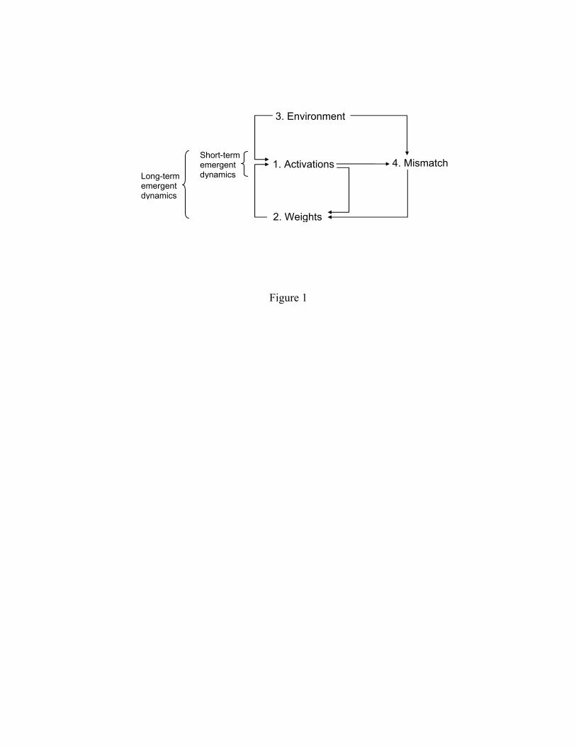
Figure 1

1. Activations

3. Environment

2. Weights

4. Mismatch Short-term emergent dynamicsLong-term

emergent dynamics

0 5 10 15 20 250

0.5

1

1.5

2

2.5

time (sec)

Uni

t Act

ivity

Figure 2

ρ1 ρ2 ρ3 ρn

. . . β

α

β β

(a) (b)

0 0.5 1−5

0

5

0 0.5 1−5

0

5

0 0.5 1−5

0

5

0 0.5 1−5

0

5

0 0.5 1−5

0

5

0 0.5 1−5

0

5

0 0.5 1−5

0

5

0 0.5 1−5

0

5

0 0.5 1−5

0

5

0 0.5 1−5

0

5

0 0.5 1−5

0

5

0 0.5 1−5

0

5

Figure 3

k= –0.2

k= +0.2

k= +0.4

β= 0 β= 0.2 β= 0.4 β= 0.6

ρ1

υ

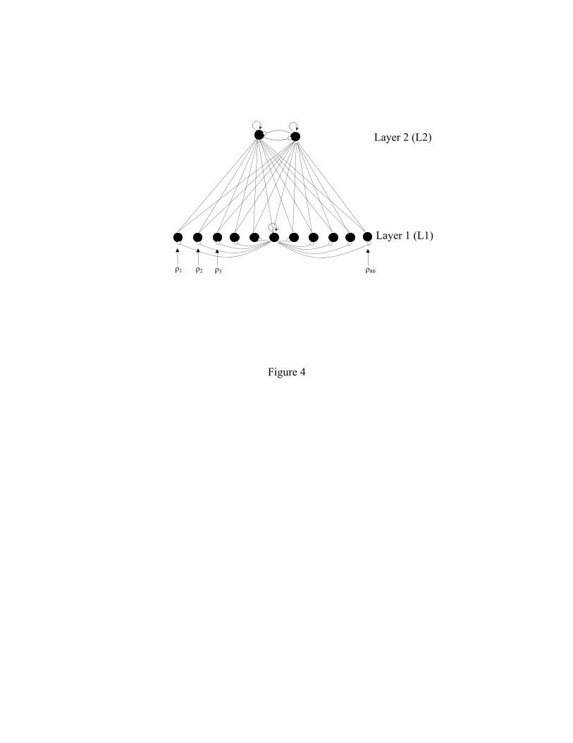
Figure 4

Layer 1 (L1)

Layer 2 (L2)

ρ1 ρ2 ρ3 ρ80

21 25 29 33 370

0.2

0.4

0.6

0.821 25 29 33 37

0

0.2

0.4

0.6

0.821 25 29 33 37

0

0.2

0.4

0.6

0.821 25 29 33 37

0

0.2

0.4

0.6

0.821 25 29 33 37

0

0.2

0.4

0.6

0.8

21 25 29 33 370

0.2

0.4

0.6

0.821 25 29 33 37

0

0.2

0.4

0.6

0.821 25 29 33 37

0

0.2

0.4

0.6

0.821 25 29 33 37

0

0.2

0.4

0.6

0.821 25 29 33 37

0

0.2

0.4

0.6

0.8

21 25 29 33 370

0.2

0.4

0.6

0.821 25 29 33 37

0

0.2

0.4

0.6

0.821 25 29 33 37

0

0.2

0.4

0.6

0.821 25 29 33 37

0

0.2

0.4

0.6

0.821 25 29 33 37

0

0.2

0.4

0.6

0.8

Figure 5

Before training After 1500 updates After 4000 updates

Inp = 25

Activity at firsttime step

Activity at final time step

Inp = 27

Inp = 29

Inp = 31

Inp = 33

L1 units

20 25 30 35 40 45 50 55 60

−2

−1

0

1

2

Input location

Ske

w

5 10 15 20 25 300

0.5

1

1.5

2

Number of timesteps

Ske

w

05001000150020004000

# of updates

Figure 6

(a)

(b)

Figure 7

fish

living thing

plant

tree flower bird

animal

ISA

ISA

ISA

ISA

ISAISAISAISAISA

ISAISAISA

pine oak rosedaisy canary

robinsunfish salmon

ISA ISA

is is is is is is is is

green tall red yellow red sing yellow yellow red

can

bark

big

roots

petalsfeathers

fly

wings

swim

gills

scales

skin

move

living

growcan

is

is

has

has

is

pretty

has has

can

has

can

has

has

has

can

salmon

sunfish

canary

robin

daisy

rose

oak

pine

skin

roots

gills

scales

feathers

wings

petals

bark

sing

yellow

fly

swim

move

grow

red

green

tall

living

pretty

salmon

sunfish

canary

robin

daisy

rose

oak

pine

flower

bird

flower

tree

animal

living thing

plant

Relation

HiddenRepresentation

Attribute

Item

ISA

is

can

has

Figure 8

pine

oak

rose

daisy

robin

canary

sunfish

salmon

Epoch 50 Epoch 100 Epoch 150

Figure 9

Fish

Bird

ANIMAL

PLANT

Tree

Flower

pine

sunfish

salmon

canary

robin

daisy

rose

oak

Figure 10

Epochs

0 500 1000 1500 2000 2500

00.

250.

50.

751

00.

250.

50

0.25

0.5

0.75

Dis

tanc

eEr

ror d

iffer

entia

lA

ctiv

atio

ncan movehas wingscan sing

Plants vs AnimalsBirds vs FishRobin vs Canary

Plants vs AnimalsBirds vs FishRobin vs Canary

Canary

is yellow

Figure 11

(a)

(b)

(c)

1st 2nd 3rd 4th 5th 6th 7th 8th

PlantRootsLeavesBranchesTreeBigBarkFlowerPrettyPetalsOakGreenPineRoseDaisyLTLivingGrowRedYellowSunfishSalmonRobinCanarySingGillsScalesFishSwimBirdFlyWingsFeathersSkinAnimalMove

Eigen Vectors

Strong negativeweighting

Strong positiveweighting

Figure 12

McClelland and Vallabha 2/26/2007 Page - Stanford...

Documents

Transcript of McClelland and Vallabha 2/26/2007 Page - Stanford...