Transportation, Assignment and

Transshipment Problems

Course: MBASubject: Quantitative

TechniquesUnit: 1.2

ApplicationsPhysical analog

of nodes Physical analog

of arcsFlow

Communicationsystems

phone exchanges, computers, transmission

facilities, satellites

Cables, fiber optic links, microwave

relay links

Voice messages, Data,

Video transmissions

Hydraulic systemsPumping stationsReservoirs, Lakes

PipelinesWater, Gas, Oil,Hydraulic fluids

Integrated computer circuits

Gates, registers,processors

Wires Electrical current

Mechanical systems JointsRods, Beams,

SpringsHeat, Energy

Transportationsystems

Intersections, Airports,Rail yards

Highways,Airline routes

Railbeds

Passengers, freight,

vehicles, operators

Applications of Network Optimization

Description

A transportation problem basically deals with the problem, which aims to find the best way to fulfill the demand of n demand points using the capacities of m supply points. While trying to find the best way, generally a variable cost of shipping the product from one supply point to a demand point or a similar constraint should be taken into consideration.

7.1 Formulating Transportation Problems

Example 1: Powerco has three electric power plants that supply the electric needs of four cities.

•The associated supply of each plant and demand of each city is given in the table 1.

•The cost of sending 1 million kwh of electricity from a plant to a city depends on the distance the electricity must travel.

Transportation tableau

A transportation problem is specified by the supply, the demand, and the shipping costs. So the relevant data can be summarized in a transportation tableau. The transportation tableau implicitly expresses the supply and demand constraints and the shipping cost between each demand and supply point.

Table 1. Shipping costs, Supply, and Demand for Powerco Example

From To

City 1 City 2 City 3 City 4 Supply

(Million kwh)

Plant 1 $8 $6 $10 $9 35

Plant 2 $9 $12 $13 $7 50

Plant 3 $14 $9 $16 $5 40

Demand

(Million kwh)

45 20 30 30

Transportation Tableau

Solution

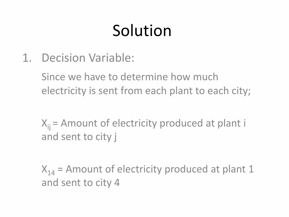
1. Decision Variable:

Since we have to determine how much electricity is sent from each plant to each city;

Xij = Amount of electricity produced at plant i and sent to city j

X14 = Amount of electricity produced at plant 1 and sent to city 4

2. Objective function

Since we want to minimize the total cost of shipping from plants to cities;

Minimize Z = 8X11+6X12+10X13+9X14

+9X21+12X22+13X23+7X24

+14X31+9X32+16X33+5X34

3. Supply Constraints

Since each supply point has a limited production capacity;

X11+X12+X13+X14 <= 35

X21+X22+X23+X24 <= 50

X31+X32+X33+X34 <= 40

4. Demand Constraints

Since each supply point has a limited production capacity;

X11+X21+X31 >= 45

X12+X22+X32 >= 20

X13+X23+X33 >= 30

X14+X24+X34 >= 30

5. Sign Constraints

Since a negative amount of electricity can not be shipped all Xij’s must be non negative;

Xij >= 0 (i= 1,2,3; j= 1,2,3,4)

LP Formulation of Powerco’s Problem

Min Z = 8X11+6X12+10X13+9X14+9X21+12X22+13X23+7X24

+14X31+9X32+16X33+5X34

S.T.: X11+X12+X13+X14 <= 35 (Supply Constraints)

X21+X22+X23+X24 <= 50

X31+X32+X33+X34 <= 40

X11+X21+X31 >= 45 (Demand Constraints)

X12+X22+X32 >= 20

X13+X23+X33 >= 30

X14+X24+X34 >= 30

Xij >= 0 (i= 1,2,3; j= 1,2,3,4)

General Description of a Transportation Problem

1. A set of m supply points from which a good is shipped. Supply point i can supply at most si

units.

2. A set of n demand points to which the good is shipped. Demand point j must receive at least di

units of the shipped good.

3. Each unit produced at supply point i and shipped to demand point j incurs a variable costof cij.

Xij = number of units shipped from supply point i to demand point j

),...,2,1;,...,2,1(0

),...,2,1(

),...,2,1(..

min

1

1

1 1

njmiX

njdX

misXts

Xc

ij

mi

i

jij

nj

j

iij

mi

i

nj

j

ijij

Balanced Transportation Problem

If Total supply equals to total demand, the problem is said to be a balanced transportation problem:

nj

j

j

mi

i

i ds11

Balancing a TP if total supply exceeds total demand

If total supply exceeds total demand, we can balance the problem by adding dummy demand point. Since shipments to the dummy demand point are not real, they are assigned a cost of zero.

Balancing a transportation problem if total supply is less than total demand

If a transportation problem has a total supply that is strictly less than total demand the problem has no feasible solution. There is no doubt that in such a case one or more of the demand will be left unmet. Generally in such situations a penalty cost is often associated with unmet demand and as one can guess this time the total penalty cost is desired to be minimum

7.2 Finding Basic Feasible Solution for TP

Unlike other Linear Programmingproblems, a balanced TP with m supplypoints and n demand points is easier tosolve, although it has m + n equalityconstraints. The reason for that is, if a setof decision variables (xij’s) satisfy all butone constraint, the values for xij’s willsatisfy that remaining constraintautomatically.

Methods to find the bfs for a balanced TP

There are three basic methods:

1. Northwest Corner Method

2. Minimum Cost Method

3. Vogel’s Method

1. Northwest Corner Method

To find the bfs by the NWC method:

Begin in the upper left (northwest) corner of thetransportation tableau and set x11 as large aspossible (here the limitations for setting x11 to alarger number, will be the demand of demandpoint 1 and the supply of supply point 1. Yourx11 value can not be greater than minimum ofthis 2 values).

According to the explanations in the previous slide we can set x11=3 (meaning demand of demand point 1 is satisfied by supply point 1).

5

6

2

3 5 2 3

3 2

6

2

X 5 2 3

After we check the east and south cells, we saw that we can go east (meaning supply point 1 still has capacity to fulfill some demand).

3 2 X

6

2

X 3 2 3

3 2 X

3 3

2

X X 2 3

After applying the same procedure, we saw that we can go south this time (meaning demand point 2 needs more supply by supply point 2).

3 2 X

3 2 1

2

X X X 3

3 2 X

3 2 1 X

2

X X X 2

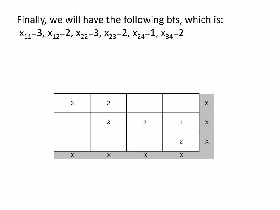
Finally, we will have the following bfs, which is:x11=3, x12=2, x22=3, x23=2, x24=1, x34=2

3 2 X

3 2 1 X

2 X

X X X X

2. Minimum Cost Method

The Northwest Corner Method dos not utilizeshipping costs. It can yield an initial bfs easily but thetotal shipping cost may be very high. The minimumcost method uses shipping costs in order come upwith a bfs that has a lower cost. To begin theminimum cost method, first we find the decisionvariable with the smallest shipping cost (Xij). Thenassign Xij its largest possible value, which is theminimum of si and dj

After that, as in the Northwest Corner Method weshould cross out row i and column j and reduce thesupply or demand of the non crossed-out row orcolumn by the value of Xij. Then we will choose thecell with the minimum cost of shipping from thecells that do not lie in a crossed-out row or columnand we will repeat the procedure.

An example for Minimum Cost MethodStep 1: Select the cell with minimum cost.

2 3 5 6

2 1 3 5

3 8 4 6

5

10

15

12 8 4 6

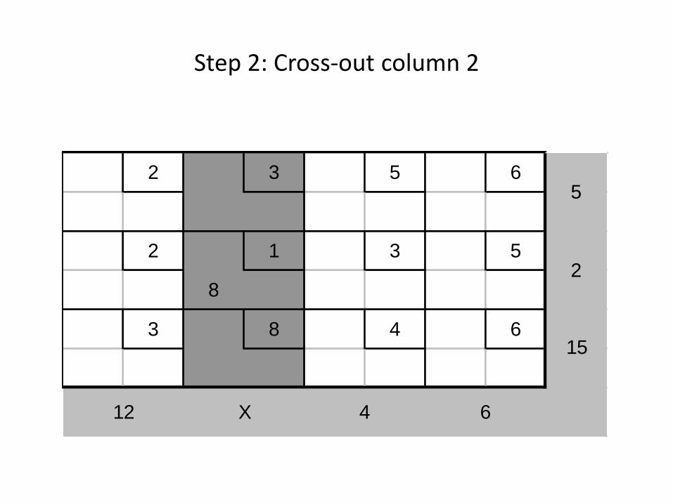
Step 2: Cross-out column 2

2 3 5 6

2 1 3 5

8

3 8 4 6

12 X 4 6

5

2

15

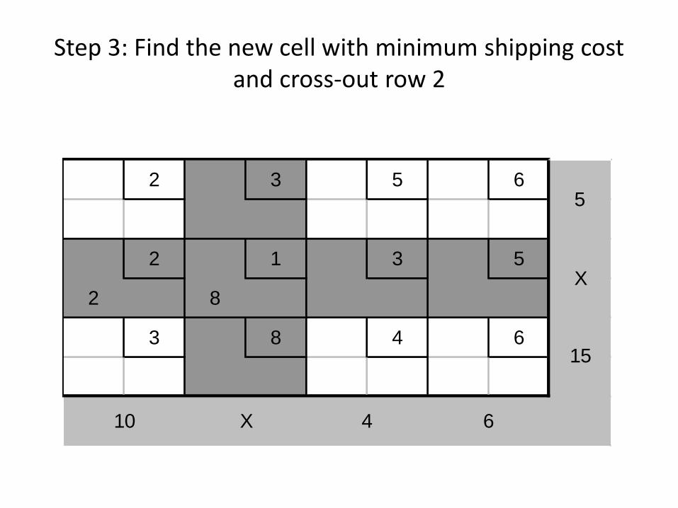
Step 3: Find the new cell with minimum shipping cost and cross-out row 2

2 3 5 6

2 1 3 5

2 8

3 8 4 6

5

X

15

10 X 4 6

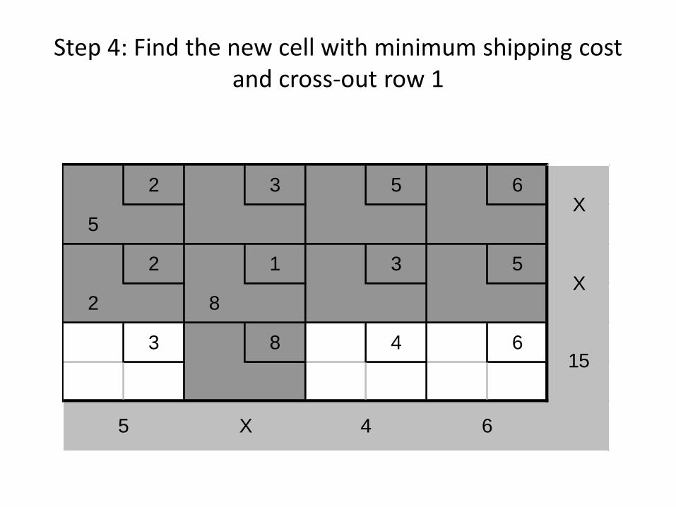
Step 4: Find the new cell with minimum shipping cost and cross-out row 1

2 3 5 6

5

2 1 3 5

2 8

3 8 4 6

X

X

15

5 X 4 6

Step 5: Find the new cell with minimum shipping cost and cross-out column 1

2 3 5 6

5

2 1 3 5

2 8

3 8 4 6

5

X

X

10

X X 4 6

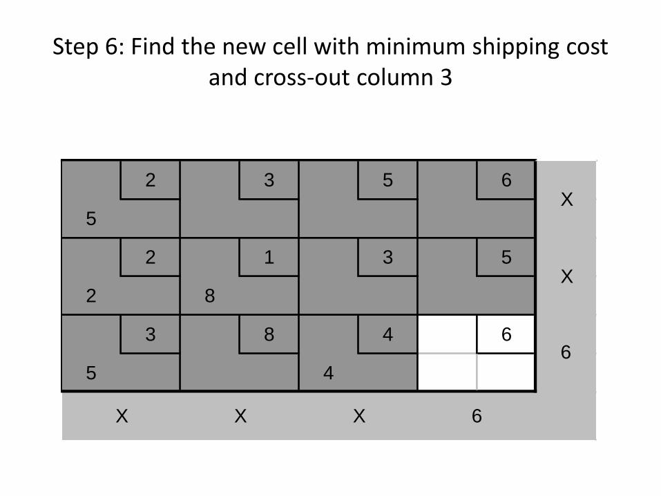
Step 6: Find the new cell with minimum shipping cost and cross-out column 3

2 3 5 6

5

2 1 3 5

2 8

3 8 4 6

5 4

X

X

6

X X X 6

Step 7: Finally assign 6 to last cell. The bfs is found as: X11=5, X21=2, X22=8, X31=5, X33=4 and X34=6

2 3 5 6

5

2 1 3 5

2 8

3 8 4 6

5 4 6

X

X

X

X X X X

3. Vogel’s Method

Begin with computing each row and column a penalty. The penalty will be equal to the difference between the two smallest shipping costs in the row or column. Identify the row or column with the largest penalty. Find the first basic variable which has the smallest shipping cost in that row or column. Then assign the highest possible value to that variable, and cross-out the row or column as in the previous methods. Compute new penalties and use the same procedure.

An example for Vogel’s MethodStep 1: Compute the penalties.

Supply Row Penalty

6 7 8

15 80 78

Demand

Column Penalty 15-6=9 80-7=73 78-8=70

7-6=1

78-15=63

15 5 5

10

15

Step 2: Identify the largest penalty and assign the highest possible value to the variable.

Supply Row Penalty

6 7 8

5

15 80 78

Demand

Column Penalty 15-6=9 _ 78-8=70

8-6=2

78-15=63

15 X 5

5

15

Step 3: Identify the largest penalty and assign the highest possible value to the variable.

Supply Row Penalty

6 7 8

5 5

15 80 78

Demand

Column Penalty 15-6=9 _ _

_

_

15 X X

0

15

Step 4: Identify the largest penalty and assign the highest possible value to the variable.

Supply Row Penalty

6 7 8

0 5 5

15 80 78

Demand

Column Penalty _ _ _

_

_

15 X X

X

15

Step 5: Finally the bfs is found as X11=0, X12=5, X13=5, and X21=15

Supply Row Penalty

6 7 8

0 5 5

15 80 78

15

Demand

Column Penalty _ _ _

_

_

X X X

X

X

7.3 The Transportation Simplex Method

In this section we will explain how the simplex algorithm is used to solve a transportation problem.

How to Pivot a Transportation Problem

Based on the transportation tableau, the following steps should be performed.

Step 1. Determine (by a criterion to be developed shortly, for example northwest corner method) the variable that should enter the basis.

Step 2. Find the loop (it can be shown that there is only one loop) involving the entering variable and some of the basic variables.

Step 3. Counting the cells in the loop, label them as even cells or odd cells.

Step 4. Find the odd cells whose variable assumes the smallest value. Call this value θ. The variable corresponding to this odd cell will leave the basis. To perform the pivot, decrease the value of each odd cell by θ and increase the value of each even cell by θ. The variables that are not in the loop remain unchanged. The pivot is now complete. If θ=0, the entering variable will equal 0, and an odd variable that has a current value of 0 will leave the basis. In this case a degenerate bfs existed before and will result after the pivot. If more than one odd cell in the loop equals θ, you may arbitrarily choose one of these odd cells to leave the basis; again a degenerate bfs will result

7.5. Assignment Problems

Example: Machine co has four jobs to be completed.Each machine must be assigned to complete one job.The time required to setup each machine forcompleting each job is shown in the table below.Machinco wants to minimize the total setup timeneeded to complete the four jobs.

Hungarian Assignment Method (HAM)• For a typical balanced assignment problem involving a certain number of

persons and an equal number of jobs, and with an objective function of

the minimization type, the method is applied as listed in the following

steps:

1. Locate the smallest cost element in each row of the cost table. Now

subtract this smallest element from each element in that row. As a

result, there shall be at least one zero in each row of this new table,

called the reduced cost table.

2. In the reduced cost table obtained, consider each column and locate

the smallest element in it. Subtract the smallest value from every other

entry in the column. As a consequence of this action, there would be at

least one zero in each of the rows and column of the second reduced

cost table.

3. Draw minimum number of horizontal and vertical line that are required

to cover all the ‘zero’ elements.

Conti…4. Select the smallest uncovered cost element. Subtract these element

from all uncovered elements including itself and add this element

to each value located at the intersection of any two lines. The cost

element through which only one line passes remain unaltered.

5. Repeat step 3 and 4 until an optimal solution is obtained.

6. Give an optimal solution, make the job assignments as indicated by the zero element.

Setup times

(Also called the cost matrix)

Time (Hours)

Job1 Job2 Job3 Job4

Machine 1 14 5 8 7

Machine 2 2 12 6 5

Machine 3 7 8 3 9

Machine 4 2 4 6 10

References

• Quantitative Techniques, by CR Kothari, Vikaspublication

• Fundamentals of Statistics by SC GutaPublisher Sultan Chand

• Quantitative Techniques in management by N.D. Vohra Publisher: Tata Mcgraw hill