Maya 2010 Getting Started
1048
Getting Started with Maya
-
Upload
codewarrior-congrejo -
Category
Documents
-
view
4.482 -
download
16
Transcript of Maya 2010 Getting Started

Getting Started with Maya
Copyright NoticeAutodesk® Maya® 2010 Software© 2009 Autodesk, Inc. All rights reserved. Except as otherwise permitted by Autodesk, Inc., this publication, or parts thereof, may not bereproduced in any form, by any method, for any purpose.Certain materials included in this publication are reprinted with the permission of the copyright holder.The following are registered trademarks or trademarks of Autodesk, Inc., and/or its subsidiaries and/or affiliates in the USA and other countries:3DEC (design/logo), 3December, 3December.com, 3ds Max, ADI, Algor, Alias, Alias (swirl design/logo), AliasStudio, Alias|Wavefront (design/logo),ATC, AUGI, AutoCAD, AutoCAD Learning Assistance, AutoCAD LT, AutoCAD Simulator, AutoCAD SQL Extension, AutoCAD SQL Interface,Autodesk, Autodesk Envision, Autodesk Intent, Autodesk Inventor, Autodesk Map, Autodesk MapGuide, Autodesk Streamline, AutoLISP, AutoSnap,AutoSketch, AutoTrack, Backburner, Backdraft, Built with ObjectARX (logo), Burn, Buzzsaw, CAiCE, Can You Imagine, Character Studio, Cinestream,Civil 3D, Cleaner, Cleaner Central, ClearScale, Colour Warper, Combustion, Communication Specification, Constructware, Content Explorer,Create>what's>Next> (design/logo), Dancing Baby (image), DesignCenter, Design Doctor, Designer's Toolkit, DesignKids, DesignProf, DesignServer,DesignStudio, Design|Studio (design/logo), Design Web Format, Discreet, DWF, DWG, DWG (logo), DWG Extreme, DWG TrueConvert, DWGTrueView, DXF, Ecotect, Exposure, Extending the Design Team, Face Robot, FBX, Fempro, Filmbox, Fire, Flame, Flint, FMDesktop, Freewheel,Frost, GDX Driver, Gmax, Green Building Studio, Heads-up Design, Heidi, HumanIK, IDEA Server, i-drop, ImageModeler, iMOUT, Incinerator,Inferno, Inventor, Inventor LT, Kaydara, Kaydara (design/logo), Kynapse, Kynogon, LandXplorer, Lustre, MatchMover, Maya, Mechanical Desktop,Moldflow, Moonbox, MotionBuilder, Movimento, MPA, MPA (design/logo), Moldflow Plastics Advisers, MPI, Moldflow Plastics Insight, MPX,MPX (design/logo), Moldflow Plastics Xpert, Mudbox, Multi-Master Editing, NavisWorks, ObjectARX, ObjectDBX, Open Reality, Opticore,Opticore Opus, Pipeplus, PolarSnap, PortfolioWall, Powered with Autodesk Technology, Productstream, ProjectPoint, ProMaterials, RasterDWG,Reactor, RealDWG, Real-time Roto, REALVIZ, Recognize, Render Queue, Retimer,Reveal, Revit, Showcase, ShowMotion, SketchBook, Smoke,Softimage, Softimage|XSI (design/logo), Sparks, SteeringWheels, Stitcher, Stone, StudioTools, Topobase, Toxik, TrustedDWG, ViewCube, Visual,Visual Construction, Visual Drainage, Visual Landscape, Visual Survey, Visual Toolbox, Visual LISP, Voice Reality, Volo, Vtour, Wire, Wiretap,WiretapCentral, XSI, and XSI (design/logo).mental ray is a registered trademark of mental images GmbH licensed for use by Autodesk, Inc. Python is a registered trademark of PythonSoftware Foundation. Adobe, Illustrator and Photoshop are either registered trademarks or trademarks of Adobe Systems Incorporated in theUnited States and/or other countries. The Ravix logo is a trademark of Electric Rain, Inc. All other brand names, product names or trademarksbelong to their respective holders.DisclaimerTHIS PUBLICATION AND THE INFORMATION CONTAINED HEREIN IS MADE AVAILABLE BY AUTODESK, INC. "AS IS." AUTODESK, INC. DISCLAIMSALL WARRANTIES, EITHER EXPRESS OR IMPLIED, INCLUDING BUT NOT LIMITED TO ANY IMPLIED WARRANTIES OF MERCHANTABILITY ORFITNESS FOR A PARTICULAR PURPOSE REGARDING THESE MATERIALS.

Contents
Chapter 1 Overview . . . . . . . . . . . . . . . . . . . . . . . . . . . . . . 1Introduction . . . . . . . . . . . . . . . . . . . . . . . . . . . . . . . . 1About the Getting Started lessons . . . . . . . . . . . . . . . . . . . . . 2Before you begin . . . . . . . . . . . . . . . . . . . . . . . . . . . . . . 3Installing Maya . . . . . . . . . . . . . . . . . . . . . . . . . . . . . . . 3Conventions used in the lessons . . . . . . . . . . . . . . . . . . . . . . 4Using the lesson files . . . . . . . . . . . . . . . . . . . . . . . . . . . . 5Using the Maya Help . . . . . . . . . . . . . . . . . . . . . . . . . . . . 5Additional learning resources . . . . . . . . . . . . . . . . . . . . . . . 10Restoring default user settings . . . . . . . . . . . . . . . . . . . . . . 11
Chapter 2 Maya Basics . . . . . . . . . . . . . . . . . . . . . . . . . . . . 13Introduction . . . . . . . . . . . . . . . . . . . . . . . . . . . . . . . . 13Preparing for the lessons . . . . . . . . . . . . . . . . . . . . . . . . . 14Lesson 1: The Maya user interface . . . . . . . . . . . . . . . . . . . . 15
Introduction . . . . . . . . . . . . . . . . . . . . . . . . . . . . . 15Starting Maya . . . . . . . . . . . . . . . . . . . . . . . . . . . . 15The Maya interface . . . . . . . . . . . . . . . . . . . . . . . . . 16Copying and setting the Maya project . . . . . . . . . . . . . . . 25Saving your work . . . . . . . . . . . . . . . . . . . . . . . . . . 26Exiting Maya . . . . . . . . . . . . . . . . . . . . . . . . . . . . 27Beyond the lesson . . . . . . . . . . . . . . . . . . . . . . . . . . 28
Lesson 2: Creating, manipulating, and viewing objects . . . . . . . . . 29
iii

Introduction . . . . . . . . . . . . . . . . . . . . . . . . . . . . . 29Creating a new scene . . . . . . . . . . . . . . . . . . . . . . . . 30Primitive objects . . . . . . . . . . . . . . . . . . . . . . . . . . . 30The Toolbox: Layout shortcuts . . . . . . . . . . . . . . . . . . . 32The Toolbox: Transformation tools . . . . . . . . . . . . . . . . . 34The Channel Box . . . . . . . . . . . . . . . . . . . . . . . . . . 37Duplicating objects . . . . . . . . . . . . . . . . . . . . . . . . . 39Save your work . . . . . . . . . . . . . . . . . . . . . . . . . . . 40Beyond the lesson . . . . . . . . . . . . . . . . . . . . . . . . . . 41
Lesson 3: Viewing the Maya 3D scene . . . . . . . . . . . . . . . . . . 42Introduction . . . . . . . . . . . . . . . . . . . . . . . . . . . . . 42Camera tools . . . . . . . . . . . . . . . . . . . . . . . . . . . . 43Workflow overview . . . . . . . . . . . . . . . . . . . . . . . . . 46Viewing objects in shaded mode . . . . . . . . . . . . . . . . . . 51Grouping objects . . . . . . . . . . . . . . . . . . . . . . . . . . 52The Hypergraph . . . . . . . . . . . . . . . . . . . . . . . . . . . 53Selection modes and masks . . . . . . . . . . . . . . . . . . . . . 56Pivot points . . . . . . . . . . . . . . . . . . . . . . . . . . . . . 57Save your work . . . . . . . . . . . . . . . . . . . . . . . . . . . 59Beyond the lesson . . . . . . . . . . . . . . . . . . . . . . . . . . 59
Lesson 4: Components and attributes . . . . . . . . . . . . . . . . . . 60Introduction . . . . . . . . . . . . . . . . . . . . . . . . . . . . . 60Template display . . . . . . . . . . . . . . . . . . . . . . . . . . 60Components . . . . . . . . . . . . . . . . . . . . . . . . . . . . . 62The Attribute Editor . . . . . . . . . . . . . . . . . . . . . . . . . 65Surface materials . . . . . . . . . . . . . . . . . . . . . . . . . . 67Save your work . . . . . . . . . . . . . . . . . . . . . . . . . . . 69Beyond the lesson . . . . . . . . . . . . . . . . . . . . . . . . . . 70
Chapter 3 Polygonal Modeling . . . . . . . . . . . . . . . . . . . . . . . . 71Introduction . . . . . . . . . . . . . . . . . . . . . . . . . . . . . . . . 71Preparing for the lesson . . . . . . . . . . . . . . . . . . . . . . . . . . 72Lesson 1: Modeling a polygonal mesh . . . . . . . . . . . . . . . . . . 73
Introduction . . . . . . . . . . . . . . . . . . . . . . . . . . . . . 73Setting modeling preferences . . . . . . . . . . . . . . . . . . . . 74Using 2D reference images . . . . . . . . . . . . . . . . . . . . . 75Creating a polygon primitive . . . . . . . . . . . . . . . . . . . . 78Modeling in shaded mode . . . . . . . . . . . . . . . . . . . . . 80Model symmetry . . . . . . . . . . . . . . . . . . . . . . . . . . 82Selecting components by painting . . . . . . . . . . . . . . . . . 83Selecting edge loops . . . . . . . . . . . . . . . . . . . . . . . . . 84Editing components in the orthographic views . . . . . . . . . . 86Editing components in the perspective view . . . . . . . . . . . . 93Drawing a polygon . . . . . . . . . . . . . . . . . . . . . . . . . 95Extruding polygon components . . . . . . . . . . . . . . . . . . 97Bridging between edges . . . . . . . . . . . . . . . . . . . . . . 102
iv | Contents
Adding polygons to a mesh . . . . . . . . . . . . . . . . . . . . 105Splitting polygon faces . . . . . . . . . . . . . . . . . . . . . . . 107Terminating edge loops . . . . . . . . . . . . . . . . . . . . . . 115Deleting construction history . . . . . . . . . . . . . . . . . . . 117Mirror copying a mesh . . . . . . . . . . . . . . . . . . . . . . . 119Working with a smoothed mesh . . . . . . . . . . . . . . . . . . 121Creasing and hardening edges on a mesh . . . . . . . . . . . . . 123Beyond the lesson . . . . . . . . . . . . . . . . . . . . . . . . . 129
Lesson 2: Sculpting a polygon mesh . . . . . . . . . . . . . . . . . . . 130Introduction . . . . . . . . . . . . . . . . . . . . . . . . . . . . 130Open the scene for the lesson . . . . . . . . . . . . . . . . . . . 131Using Soft Select . . . . . . . . . . . . . . . . . . . . . . . . . . 131Selecting with Camera based selection . . . . . . . . . . . . . . 135Sculpting with symmetry . . . . . . . . . . . . . . . . . . . . . 137Sculpting with Surface based falloff . . . . . . . . . . . . . . . . 141Selecting with Drag select . . . . . . . . . . . . . . . . . . . . . 143Adjusting the Seam tolerance . . . . . . . . . . . . . . . . . . . 146Beyond the lesson . . . . . . . . . . . . . . . . . . . . . . . . . 147
Chapter 4 NURBS Modeling . . . . . . . . . . . . . . . . . . . . . . . . . 149Introduction . . . . . . . . . . . . . . . . . . . . . . . . . . . . . . . 149Preparing for the lessons . . . . . . . . . . . . . . . . . . . . . . . . . 149Lesson 1: Revolving a curve to create a surface . . . . . . . . . . . . . 150
Introduction . . . . . . . . . . . . . . . . . . . . . . . . . . . . 150Creating a profile curve . . . . . . . . . . . . . . . . . . . . . . 151Creating a revolve surface . . . . . . . . . . . . . . . . . . . . . 153Editing a revolve surface . . . . . . . . . . . . . . . . . . . . . . 153Beyond the lesson . . . . . . . . . . . . . . . . . . . . . . . . . 155
Lesson 2: Sculpting a NURBS surface . . . . . . . . . . . . . . . . . . 156Introduction . . . . . . . . . . . . . . . . . . . . . . . . . . . . 156Preparing a surface for sculpting . . . . . . . . . . . . . . . . . . 157Basic sculpting techniques . . . . . . . . . . . . . . . . . . . . . 159Additional sculpting techniques . . . . . . . . . . . . . . . . . . 162Sculpting a nose . . . . . . . . . . . . . . . . . . . . . . . . . . 164Sculpting eye sockets . . . . . . . . . . . . . . . . . . . . . . . 165Sculpting eyebrows . . . . . . . . . . . . . . . . . . . . . . . . 166Sculpting a mouth . . . . . . . . . . . . . . . . . . . . . . . . . 167Sculpting other facial features . . . . . . . . . . . . . . . . . . . 169Beyond the lesson . . . . . . . . . . . . . . . . . . . . . . . . . 170
Lesson 3: Lofting curves to create a surface . . . . . . . . . . . . . . . 171Introduction . . . . . . . . . . . . . . . . . . . . . . . . . . . . 171Creating profile curves for a surface . . . . . . . . . . . . . . . . 172Duplicating curves . . . . . . . . . . . . . . . . . . . . . . . . . 174Lofting a surface . . . . . . . . . . . . . . . . . . . . . . . . . . 175Modifying a primitive object . . . . . . . . . . . . . . . . . . . 176Using the Outliner to parent objects . . . . . . . . . . . . . . . 178
Contents | v
Beyond the lesson . . . . . . . . . . . . . . . . . . . . . . . . . 179
Chapter 5 Subdivision Surfaces . . . . . . . . . . . . . . . . . . . . . . . 181Introduction . . . . . . . . . . . . . . . . . . . . . . . . . . . . . . . 181Preparing for the lesson . . . . . . . . . . . . . . . . . . . . . . . . . 181Lesson 1: Modeling a subdivision surface . . . . . . . . . . . . . . . . 182
Introduction . . . . . . . . . . . . . . . . . . . . . . . . . . . . 182Creating a subdivision surface . . . . . . . . . . . . . . . . . . . 183Splitting a surface in polygon proxy mode . . . . . . . . . . . . 185Extruding polygon faces . . . . . . . . . . . . . . . . . . . . . . 187Deleting polygon faces . . . . . . . . . . . . . . . . . . . . . . . 190Subdivision surface levels . . . . . . . . . . . . . . . . . . . . . 191Refining surface components . . . . . . . . . . . . . . . . . . . 193Creating a crease in a subdivision surface . . . . . . . . . . . . . 195Beyond the lesson . . . . . . . . . . . . . . . . . . . . . . . . . 197
Chapter 6 Animation . . . . . . . . . . . . . . . . . . . . . . . . . . . . 199Introduction . . . . . . . . . . . . . . . . . . . . . . . . . . . . . . . 199Preparing for the lessons . . . . . . . . . . . . . . . . . . . . . . . . . 199Lesson 1: Keyframes and the Graph Editor . . . . . . . . . . . . . . . 200
Introduction . . . . . . . . . . . . . . . . . . . . . . . . . . . . 200Setting the playback range . . . . . . . . . . . . . . . . . . . . . 201Setting keyframes . . . . . . . . . . . . . . . . . . . . . . . . . 202Using the Graph Editor . . . . . . . . . . . . . . . . . . . . . . 205Changing the timing of an attribute . . . . . . . . . . . . . . . 209Fine tuning an animation . . . . . . . . . . . . . . . . . . . . . 210Deleting extra keyframes and static channels . . . . . . . . . . . 212Using Playblast to playback an animation . . . . . . . . . . . . 213Beyond the lesson . . . . . . . . . . . . . . . . . . . . . . . . . 213
Lesson 2: Set Driven Key . . . . . . . . . . . . . . . . . . . . . . . . . 215Introduction . . . . . . . . . . . . . . . . . . . . . . . . . . . . 215Lesson setup . . . . . . . . . . . . . . . . . . . . . . . . . . . . 215Using Set Driven Key to link attributes . . . . . . . . . . . . . . 216Viewing the results in the Graph Editor . . . . . . . . . . . . . . 219Beyond the lesson . . . . . . . . . . . . . . . . . . . . . . . . . 219
Lesson 3: Path animation . . . . . . . . . . . . . . . . . . . . . . . . 220Introduction . . . . . . . . . . . . . . . . . . . . . . . . . . . . 220Open the scene for the lesson . . . . . . . . . . . . . . . . . . . 221Animating an object along a motion path . . . . . . . . . . . . 222Changing the timing of an object along a motion path . . . . . 224Rotating an object along a motion path . . . . . . . . . . . . . 230Blending keyframe and motion path animation . . . . . . . . . 231Using Playblast to playback an animation . . . . . . . . . . . . 237Beyond the lesson . . . . . . . . . . . . . . . . . . . . . . . . . 238
Lesson 4: Nonlinear animation with Trax . . . . . . . . . . . . . . . . 239
vi | Contents
Introduction . . . . . . . . . . . . . . . . . . . . . . . . . . . . 239Open the first scene for the lesson . . . . . . . . . . . . . . . . 240Creating clips with Trax . . . . . . . . . . . . . . . . . . . . . . 242Changing the position of clips with Trax . . . . . . . . . . . . . 249Editing the animation of clips . . . . . . . . . . . . . . . . . . . 251Reusing clips within Trax . . . . . . . . . . . . . . . . . . . . . 253Soloing and muting tracks . . . . . . . . . . . . . . . . . . . . . 256Scaling clips within Trax . . . . . . . . . . . . . . . . . . . . . . 257Open the second scene for the lesson . . . . . . . . . . . . . . . 259Creating clips from motion capture data . . . . . . . . . . . . . 260Extending the length of motion capture data . . . . . . . . . . . 261Redirecting the motion within a clip . . . . . . . . . . . . . . . 266Beyond the lesson . . . . . . . . . . . . . . . . . . . . . . . . . 273
Lesson 5: Inverse kinematics . . . . . . . . . . . . . . . . . . . . . . . 276Introduction . . . . . . . . . . . . . . . . . . . . . . . . . . . . 276Open the scene for the lesson . . . . . . . . . . . . . . . . . . . 277Understanding hierarchies . . . . . . . . . . . . . . . . . . . . . 278Viewing hierarchies using the Hypergraph . . . . . . . . . . . . 279Creating a skeleton hierarchy . . . . . . . . . . . . . . . . . . . 281Parenting a model into a skeleton hierarchy . . . . . . . . . . . 285Applying IK to a skeleton hierarchy . . . . . . . . . . . . . . . . 288Creating a control object for an IK system . . . . . . . . . . . . 290Constraining an IK system . . . . . . . . . . . . . . . . . . . . . 294Limiting the range of motion of an IK system . . . . . . . . . . 298Simplifying the display of a hierarchy . . . . . . . . . . . . . . . 304Applying parent constraints on an IK system . . . . . . . . . . . 305Planning an animation for an IK system . . . . . . . . . . . . . 308Animating an IK system . . . . . . . . . . . . . . . . . . . . . . 311Beyond the lesson . . . . . . . . . . . . . . . . . . . . . . . . . 315
Chapter 7 Character Setup . . . . . . . . . . . . . . . . . . . . . . . . . 317Introduction . . . . . . . . . . . . . . . . . . . . . . . . . . . . . . . 317Preparing for the lessons . . . . . . . . . . . . . . . . . . . . . . . . . 318Lesson 1: Skeletons and kinematics . . . . . . . . . . . . . . . . . . . 318
Introduction . . . . . . . . . . . . . . . . . . . . . . . . . . . . 318Open the scene for the lesson . . . . . . . . . . . . . . . . . . . 319Creating joints . . . . . . . . . . . . . . . . . . . . . . . . . . . 319Adding joints to a skeleton . . . . . . . . . . . . . . . . . . . . 325Creating a skeleton hierarchy . . . . . . . . . . . . . . . . . . . 327Forward and inverse kinematics . . . . . . . . . . . . . . . . . . 327Posing and animating using inverse kinematics . . . . . . . . . 328Posing and animating using forward kinematics . . . . . . . . . 332Beyond the lesson . . . . . . . . . . . . . . . . . . . . . . . . . 332
Lesson 2: Smooth skinning . . . . . . . . . . . . . . . . . . . . . . . 333Introduction . . . . . . . . . . . . . . . . . . . . . . . . . . . . 333Open the scene for the lesson . . . . . . . . . . . . . . . . . . . 334
Contents | vii

Smooth binding a skeleton . . . . . . . . . . . . . . . . . . . . 334Skin weighting and deformations . . . . . . . . . . . . . . . . . 336Modifying skin weights . . . . . . . . . . . . . . . . . . . . . . 338Influence objects . . . . . . . . . . . . . . . . . . . . . . . . . . 340Beyond the lesson . . . . . . . . . . . . . . . . . . . . . . . . . 343
Lesson 3: Cluster and blend shape deformers . . . . . . . . . . . . . . 344Introduction . . . . . . . . . . . . . . . . . . . . . . . . . . . . 344Open the scene for the lesson . . . . . . . . . . . . . . . . . . . 344Creating a target object for a blend shape . . . . . . . . . . . . . 345Creating a cluster deformer on a target object . . . . . . . . . . 346Editing cluster weights . . . . . . . . . . . . . . . . . . . . . . . 348Creating a blend shape . . . . . . . . . . . . . . . . . . . . . . 352Refining deformation effects . . . . . . . . . . . . . . . . . . . 354Adding target objects to an existing blend shape . . . . . . . . . 355Beyond the lesson . . . . . . . . . . . . . . . . . . . . . . . . . 359
Chapter 8 Polygon Texturing . . . . . . . . . . . . . . . . . . . . . . . . 361Introduction . . . . . . . . . . . . . . . . . . . . . . . . . . . . . . . 361Preparing for the lesson . . . . . . . . . . . . . . . . . . . . . . . . . 362Lesson 1: UV texture mapping . . . . . . . . . . . . . . . . . . . . . . 363
Introduction . . . . . . . . . . . . . . . . . . . . . . . . . . . . 363Creating a cracker box model . . . . . . . . . . . . . . . . . . . 364Applying a texture map to a polygon mesh . . . . . . . . . . . . 365Viewing UVs in the UV Texture Editor . . . . . . . . . . . . . . 371Mapping UV texture coordinates . . . . . . . . . . . . . . . . . 375Working with UVs in the UV Texture Editor . . . . . . . . . . . 379Beyond the lesson . . . . . . . . . . . . . . . . . . . . . . . . . 387
Lesson 2: UV unfolding . . . . . . . . . . . . . . . . . . . . . . . . . 389Introduction . . . . . . . . . . . . . . . . . . . . . . . . . . . . 389Lesson Setup . . . . . . . . . . . . . . . . . . . . . . . . . . . . 390Dividing the mesh . . . . . . . . . . . . . . . . . . . . . . . . . 391Creating a planar mapping . . . . . . . . . . . . . . . . . . . . 395Unfolding a UV mesh . . . . . . . . . . . . . . . . . . . . . . . 397Adjusting the checker pattern . . . . . . . . . . . . . . . . . . . 401Outputting UVs . . . . . . . . . . . . . . . . . . . . . . . . . . 402Unfolding with constraints . . . . . . . . . . . . . . . . . . . . 404Sewing UV Edges . . . . . . . . . . . . . . . . . . . . . . . . . . 411Smoothing/Relaxing a mesh interactively . . . . . . . . . . . . . 416Fixing problem areas . . . . . . . . . . . . . . . . . . . . . . . . 417Applying Textures . . . . . . . . . . . . . . . . . . . . . . . . . 423Beyond the lesson . . . . . . . . . . . . . . . . . . . . . . . . . 427
Lesson 3: Normal mapping . . . . . . . . . . . . . . . . . . . . . . . 428Introduction . . . . . . . . . . . . . . . . . . . . . . . . . . . . 428Lesson setup . . . . . . . . . . . . . . . . . . . . . . . . . . . . 429Open the scene for the lesson . . . . . . . . . . . . . . . . . . . 430Creating a Normal Map . . . . . . . . . . . . . . . . . . . . . . 432
viii | Contents
Viewing a normal map . . . . . . . . . . . . . . . . . . . . . . . 435Beyond the lesson . . . . . . . . . . . . . . . . . . . . . . . . . 436
Chapter 9 Rendering . . . . . . . . . . . . . . . . . . . . . . . . . . . . 437Introduction . . . . . . . . . . . . . . . . . . . . . . . . . . . . . . . 437Preparing for the lessons . . . . . . . . . . . . . . . . . . . . . . . . . 439Lesson 1: Rendering a scene . . . . . . . . . . . . . . . . . . . . . . . 439
Introduction . . . . . . . . . . . . . . . . . . . . . . . . . . . . 439Open the scene for the lesson . . . . . . . . . . . . . . . . . . . 440Creating shading materials for objects . . . . . . . . . . . . . . 441Refining shading materials for objects . . . . . . . . . . . . . . 445Maya renderers . . . . . . . . . . . . . . . . . . . . . . . . . . . 450Rendering a single frame using IPR . . . . . . . . . . . . . . . . 452Rendering using the Maya software renderer . . . . . . . . . . . 457Batch rendering a sequence of animation frames . . . . . . . . . 459Viewing a sequence of rendered frames . . . . . . . . . . . . . . 462Beyond the lesson . . . . . . . . . . . . . . . . . . . . . . . . . 463
Lesson 2: Shading surfaces . . . . . . . . . . . . . . . . . . . . . . . . 465Introduction . . . . . . . . . . . . . . . . . . . . . . . . . . . . 465Open the scene for the lesson . . . . . . . . . . . . . . . . . . . 466Assigning a shading material . . . . . . . . . . . . . . . . . . . 467Modifying surface specularity . . . . . . . . . . . . . . . . . . . 469Material types . . . . . . . . . . . . . . . . . . . . . . . . . . . 470Assigning textures . . . . . . . . . . . . . . . . . . . . . . . . . 471Using the Hypershade editor . . . . . . . . . . . . . . . . . . . 474Creating a texture within the Hypershade editor . . . . . . . . . 477Modifying a bump texture . . . . . . . . . . . . . . . . . . . . . 480Beyond the lesson . . . . . . . . . . . . . . . . . . . . . . . . . 482
Lesson 3: Lights, shadows, and cameras . . . . . . . . . . . . . . . . . 484Introduction . . . . . . . . . . . . . . . . . . . . . . . . . . . . 484Open the scene for the lesson . . . . . . . . . . . . . . . . . . . 485Directional lights . . . . . . . . . . . . . . . . . . . . . . . . . . 486Spotlights . . . . . . . . . . . . . . . . . . . . . . . . . . . . . 488Editing light attributes . . . . . . . . . . . . . . . . . . . . . . . 491Shadows . . . . . . . . . . . . . . . . . . . . . . . . . . . . . . 494Creating additional cameras in a scene . . . . . . . . . . . . . . 496Animating camera moves . . . . . . . . . . . . . . . . . . . . . 498Beyond the lesson . . . . . . . . . . . . . . . . . . . . . . . . . 499
Lesson 4: Global Illumination . . . . . . . . . . . . . . . . . . . . . . 501Introduction . . . . . . . . . . . . . . . . . . . . . . . . . . . . 501Open the scene for the lesson . . . . . . . . . . . . . . . . . . . 502Render the scene using raytracing . . . . . . . . . . . . . . . . . 503Render the scene using Global Illumination . . . . . . . . . . . 508Beyond the Lesson . . . . . . . . . . . . . . . . . . . . . . . . . 517
Lesson 5: Caustics . . . . . . . . . . . . . . . . . . . . . . . . . . . . 519Introduction . . . . . . . . . . . . . . . . . . . . . . . . . . . . 519
Contents | ix
Open the scene for the lesson . . . . . . . . . . . . . . . . . . . 520Render the scene using raytracing . . . . . . . . . . . . . . . . . 521Render the scene using caustics . . . . . . . . . . . . . . . . . . 526Beyond the Lesson . . . . . . . . . . . . . . . . . . . . . . . . . 532
Chapter 10 Dynamics . . . . . . . . . . . . . . . . . . . . . . . . . . . . . 535Introduction . . . . . . . . . . . . . . . . . . . . . . . . . . . . . . . 535Preparing for the lessons . . . . . . . . . . . . . . . . . . . . . . . . . 535Lesson 1: Particles, emitters, and fields . . . . . . . . . . . . . . . . . 536
Introduction . . . . . . . . . . . . . . . . . . . . . . . . . . . . 536Creating an emitter . . . . . . . . . . . . . . . . . . . . . . . . 537Creating volume axis fields . . . . . . . . . . . . . . . . . . . . 539Adjusting the velocity of moving particles . . . . . . . . . . . . 545Setting the particle render type . . . . . . . . . . . . . . . . . . 545Adding dynamic attributes . . . . . . . . . . . . . . . . . . . . 546Adding per particle attributes . . . . . . . . . . . . . . . . . . . 548Adding color to particles with a color ramp . . . . . . . . . . . 549Hardware rendering particles . . . . . . . . . . . . . . . . . . . 551Beyond the lesson . . . . . . . . . . . . . . . . . . . . . . . . . 553
Lesson 2: Rigid bodies and constraints . . . . . . . . . . . . . . . . . 554Introduction . . . . . . . . . . . . . . . . . . . . . . . . . . . . 554Lesson setup . . . . . . . . . . . . . . . . . . . . . . . . . . . . 554Creating hinge constraints . . . . . . . . . . . . . . . . . . . . . 556Running a dynamics simulation . . . . . . . . . . . . . . . . . . 557Changing an active rigid body to passive . . . . . . . . . . . . . 558Beyond the lesson . . . . . . . . . . . . . . . . . . . . . . . . . 559
Chapter 11 Painting . . . . . . . . . . . . . . . . . . . . . . . . . . . . . 561Introduction . . . . . . . . . . . . . . . . . . . . . . . . . . . . . . . 561Preparing for the lessons . . . . . . . . . . . . . . . . . . . . . . . . . 562Lesson 1: Painting in 2D using Paint Effects . . . . . . . . . . . . . . 563
Introduction . . . . . . . . . . . . . . . . . . . . . . . . . . . . 563Painting strokes . . . . . . . . . . . . . . . . . . . . . . . . . . 564Modifying the default brush settings . . . . . . . . . . . . . . . 566Modifying the canvas . . . . . . . . . . . . . . . . . . . . . . . 568Modifying the colors of a preset brush . . . . . . . . . . . . . . 568Editing strokes with tubes attributes . . . . . . . . . . . . . . . 570Saving brush settings for future use . . . . . . . . . . . . . . . . 571Blending brushes . . . . . . . . . . . . . . . . . . . . . . . . . . 572Smearing, blurring, and erasing paint . . . . . . . . . . . . . . . 573Beyond the lesson . . . . . . . . . . . . . . . . . . . . . . . . . 574
Lesson 2: Painting in 3D using Paint Effects . . . . . . . . . . . . . . 575Introduction . . . . . . . . . . . . . . . . . . . . . . . . . . . . 575Preparing for the lessons . . . . . . . . . . . . . . . . . . . . . . 576Brushes and strokes . . . . . . . . . . . . . . . . . . . . . . . . 577
x | Contents

Rendering Paint Effects strokes . . . . . . . . . . . . . . . . . . 584Paint Effects on 3D objects . . . . . . . . . . . . . . . . . . . . 589Creating a surface to paint on . . . . . . . . . . . . . . . . . . . 590Painting on objects . . . . . . . . . . . . . . . . . . . . . . . . 593Using turbulence with brush stroke tubes . . . . . . . . . . . . . 595Using additional preset brushes . . . . . . . . . . . . . . . . . . 596Mesh brushes . . . . . . . . . . . . . . . . . . . . . . . . . . . . 598Converting mesh strokes to polygons . . . . . . . . . . . . . . . 600Modifying a converted polygonal mesh . . . . . . . . . . . . . . 602Beyond the lesson . . . . . . . . . . . . . . . . . . . . . . . . . 606
Lesson 3: Painting textures on surfaces . . . . . . . . . . . . . . . . . 608Introduction . . . . . . . . . . . . . . . . . . . . . . . . . . . . 608Open the scene for the lesson . . . . . . . . . . . . . . . . . . . 608Preparing for painting . . . . . . . . . . . . . . . . . . . . . . . 609Painting with an Artisan brush . . . . . . . . . . . . . . . . . . 611Painting symmetrical strokes . . . . . . . . . . . . . . . . . . . 612Using Flood All to apply a single color . . . . . . . . . . . . . . 613Brush shapes . . . . . . . . . . . . . . . . . . . . . . . . . . . . 613Painting with a Paint Effects brush . . . . . . . . . . . . . . . . 615Smearing and blurring . . . . . . . . . . . . . . . . . . . . . . . 617Painting a bump map texture . . . . . . . . . . . . . . . . . . . 618Beyond the lesson . . . . . . . . . . . . . . . . . . . . . . . . . 621
Chapter 12 Expressions . . . . . . . . . . . . . . . . . . . . . . . . . . . . 625Introduction . . . . . . . . . . . . . . . . . . . . . . . . . . . . . . . 625Preparing for the lessons . . . . . . . . . . . . . . . . . . . . . . . . . 626Lesson 1: Creating a simple expression . . . . . . . . . . . . . . . . . 627
Introduction . . . . . . . . . . . . . . . . . . . . . . . . . . . . 627Creating expressions to control a single attribute . . . . . . . . . 627Editing expressions . . . . . . . . . . . . . . . . . . . . . . . . 630Using expressions to control multiple attributes . . . . . . . . . 631Linking multiple attributes on the same object . . . . . . . . . . 631Controlling attributes in two objects . . . . . . . . . . . . . . . 632Beyond the lesson . . . . . . . . . . . . . . . . . . . . . . . . . 632
Lesson 2: Conditional expressions . . . . . . . . . . . . . . . . . . . . 634Introduction . . . . . . . . . . . . . . . . . . . . . . . . . . . . 634Creating a conditional expression . . . . . . . . . . . . . . . . . 634Other conditional statement options . . . . . . . . . . . . . . . 637Fixing a problem in an expression . . . . . . . . . . . . . . . . . 639Using else statements . . . . . . . . . . . . . . . . . . . . . . . 639Simplifying expressions . . . . . . . . . . . . . . . . . . . . . . 640Editing expressions to refine an animation . . . . . . . . . . . . 641Beyond the lesson . . . . . . . . . . . . . . . . . . . . . . . . . 643
Lesson 3: Controlling particle attributes . . . . . . . . . . . . . . . . 643Introduction . . . . . . . . . . . . . . . . . . . . . . . . . . . . 643Creating particle objects . . . . . . . . . . . . . . . . . . . . . . 644
Contents | xi

Using creation expressions to set a constant color . . . . . . . . 645Using runtime expressions . . . . . . . . . . . . . . . . . . . . . 646Modifying runtime expressions . . . . . . . . . . . . . . . . . . 648Beyond the lesson . . . . . . . . . . . . . . . . . . . . . . . . . 649
Chapter 13 Scripting in Maya . . . . . . . . . . . . . . . . . . . . . . . . 651Introduction . . . . . . . . . . . . . . . . . . . . . . . . . . . . . . . 651Some basic concepts . . . . . . . . . . . . . . . . . . . . . . . . . . . 652Preparing for the lessons . . . . . . . . . . . . . . . . . . . . . . . . . 655Lesson 1: Commands in MEL . . . . . . . . . . . . . . . . . . . . . . 656
Introduction . . . . . . . . . . . . . . . . . . . . . . . . . . . . 656Entering MEL commands . . . . . . . . . . . . . . . . . . . . . 657Observing script history . . . . . . . . . . . . . . . . . . . . . . 658Modifying object attributes . . . . . . . . . . . . . . . . . . . . 661Editing Objects . . . . . . . . . . . . . . . . . . . . . . . . . . . 664Beyond the lesson . . . . . . . . . . . . . . . . . . . . . . . . . 665
Lesson 2: Saving scripts to the Shelf . . . . . . . . . . . . . . . . . . . 666Introduction . . . . . . . . . . . . . . . . . . . . . . . . . . . . 666Setting up the scene . . . . . . . . . . . . . . . . . . . . . . . . 667Recording the script history . . . . . . . . . . . . . . . . . . . . 668Compare the rendered images . . . . . . . . . . . . . . . . . . 670Saving the history as a button . . . . . . . . . . . . . . . . . . . 671Beyond the Lesson . . . . . . . . . . . . . . . . . . . . . . . . . 673
Lesson 3: Using Variables in MEL . . . . . . . . . . . . . . . . . . . . 674Introduction . . . . . . . . . . . . . . . . . . . . . . . . . . . . 674Setting up the scene . . . . . . . . . . . . . . . . . . . . . . . . 674Storing scene information . . . . . . . . . . . . . . . . . . . . . 675Create a row of barrels . . . . . . . . . . . . . . . . . . . . . . . 677Stacking the row of barrels . . . . . . . . . . . . . . . . . . . . . 678Using MEL built-in functions to calculate the Y offset . . . . . . 679Creating dynamics with MEL commands . . . . . . . . . . . . . 681Beyond the lesson . . . . . . . . . . . . . . . . . . . . . . . . . 683
Lesson 4: User interface creation and procedures . . . . . . . . . . . . 683Introduction . . . . . . . . . . . . . . . . . . . . . . . . . . . . 683Creating a window . . . . . . . . . . . . . . . . . . . . . . . . . 684Window naming . . . . . . . . . . . . . . . . . . . . . . . . . . 686Introduction to procedures . . . . . . . . . . . . . . . . . . . . 689Loading a script file . . . . . . . . . . . . . . . . . . . . . . . . 691Linking the user interface . . . . . . . . . . . . . . . . . . . . . 695Saving the script . . . . . . . . . . . . . . . . . . . . . . . . . . 700Using the saved script file . . . . . . . . . . . . . . . . . . . . . 701Beyond the lesson . . . . . . . . . . . . . . . . . . . . . . . . . 702
Lesson 5: Using Python in Maya . . . . . . . . . . . . . . . . . . . . 703Introduction . . . . . . . . . . . . . . . . . . . . . . . . . . . . 703Entering Python commands . . . . . . . . . . . . . . . . . . . . 704Using flags in Python . . . . . . . . . . . . . . . . . . . . . . . 707
xii | Contents

Using the edit flag in Python . . . . . . . . . . . . . . . . . . . 711Communicating between Python and MEL . . . . . . . . . . . . 713Beyond the lesson . . . . . . . . . . . . . . . . . . . . . . . . . 715
Chapter 14 Assets . . . . . . . . . . . . . . . . . . . . . . . . . . . . . . . 717Introduction . . . . . . . . . . . . . . . . . . . . . . . . . . . . . . . 717Preparing for the lessons . . . . . . . . . . . . . . . . . . . . . . . . . 717Lesson 1: Setting up an asset . . . . . . . . . . . . . . . . . . . . . . . 718
Introduction . . . . . . . . . . . . . . . . . . . . . . . . . . . . 718Lesson setup . . . . . . . . . . . . . . . . . . . . . . . . . . . . 718Creating a container . . . . . . . . . . . . . . . . . . . . . . . . 719Publishing attributes . . . . . . . . . . . . . . . . . . . . . . . . 720Publishing multiple attributes to a single published name . . . . 722Open the second scene for the lesson . . . . . . . . . . . . . . . 725Creating a template . . . . . . . . . . . . . . . . . . . . . . . . 725Creating Views . . . . . . . . . . . . . . . . . . . . . . . . . . . 727Assigning a custom icon . . . . . . . . . . . . . . . . . . . . . . 730Setting Black Box mode . . . . . . . . . . . . . . . . . . . . . . 731Beyond the lesson . . . . . . . . . . . . . . . . . . . . . . . . . 732
Lesson 2: Using assets in a scene . . . . . . . . . . . . . . . . . . . . . 732Introduction . . . . . . . . . . . . . . . . . . . . . . . . . . . . 732Lesson setup . . . . . . . . . . . . . . . . . . . . . . . . . . . . 733Importing assets to dress a scene . . . . . . . . . . . . . . . . . 734Assigning an existing template to a container . . . . . . . . . . 735Binding attributes . . . . . . . . . . . . . . . . . . . . . . . . . 738Swapping assets . . . . . . . . . . . . . . . . . . . . . . . . . . 740Referencing assets in a scene . . . . . . . . . . . . . . . . . . . . 742Creating a proxy container . . . . . . . . . . . . . . . . . . . . 745Modifying a proxy container . . . . . . . . . . . . . . . . . . . 747Dressing the rest of the scene with assets . . . . . . . . . . . . . 749Beyond the lesson . . . . . . . . . . . . . . . . . . . . . . . . . 751
Chapter 15 Hair . . . . . . . . . . . . . . . . . . . . . . . . . . . . . . . . 753Introduction . . . . . . . . . . . . . . . . . . . . . . . . . . . . . . . 753About hair simulation . . . . . . . . . . . . . . . . . . . . . . . . . . 755Preparing for the lessons . . . . . . . . . . . . . . . . . . . . . . . . . 755Lesson 1: Creating a basic hairstyle . . . . . . . . . . . . . . . . . . . 756
Introduction . . . . . . . . . . . . . . . . . . . . . . . . . . . . 756Lesson setup . . . . . . . . . . . . . . . . . . . . . . . . . . . . 757Creating hair on a surface . . . . . . . . . . . . . . . . . . . . . 758Styling the hair . . . . . . . . . . . . . . . . . . . . . . . . . . . 762Setting up hair collisions . . . . . . . . . . . . . . . . . . . . . 767Rendering the hair . . . . . . . . . . . . . . . . . . . . . . . . . 771Modifying hair attributes . . . . . . . . . . . . . . . . . . . . . 772Setting up shadowing on hair . . . . . . . . . . . . . . . . . . . 774
Contents | xiii

Beyond the lesson . . . . . . . . . . . . . . . . . . . . . . . . . 776Lesson 2: Creating a dynamic non-hair simulation . . . . . . . . . . . 777
Introduction . . . . . . . . . . . . . . . . . . . . . . . . . . . . 777Lesson setup . . . . . . . . . . . . . . . . . . . . . . . . . . . . 778Setting up the curtain scene . . . . . . . . . . . . . . . . . . . . 778Making the hair collide with another object . . . . . . . . . . . 782Assigning a Paint Effects brush to the hair . . . . . . . . . . . . 782Setting up constraints . . . . . . . . . . . . . . . . . . . . . . . 784Rendering the curtain scene . . . . . . . . . . . . . . . . . . . . 786Beyond the lesson . . . . . . . . . . . . . . . . . . . . . . . . . 787
Chapter 16 Fluid Effects . . . . . . . . . . . . . . . . . . . . . . . . . . . 789Introduction . . . . . . . . . . . . . . . . . . . . . . . . . . . . . . . 789Preparing for the lessons . . . . . . . . . . . . . . . . . . . . . . . . . 790Lesson 1: Creating a dynamic 2D fluid effect . . . . . . . . . . . . . . 791
Introduction . . . . . . . . . . . . . . . . . . . . . . . . . . . . 791Creating a two-dimensional fluid container . . . . . . . . . . . 792Adding a fluid emitter to a container . . . . . . . . . . . . . . . 792Changing the behavior of a fluid . . . . . . . . . . . . . . . . . 794Combining colors in a fluid . . . . . . . . . . . . . . . . . . . . 797Colliding a fluid with an object . . . . . . . . . . . . . . . . . . 798Beyond the lesson . . . . . . . . . . . . . . . . . . . . . . . . . 800
Lesson 2: Creating a non-dynamic 3D fluid effect . . . . . . . . . . . 801Introduction . . . . . . . . . . . . . . . . . . . . . . . . . . . . 801Creating a 3D fluid container . . . . . . . . . . . . . . . . . . . 801Adding fluid to a container . . . . . . . . . . . . . . . . . . . . 803Defining shader attributes for a fluid . . . . . . . . . . . . . . . 803Texturing the contents of a fluid container . . . . . . . . . . . . 804Adding self shadowing to texture density . . . . . . . . . . . . . 808Beyond the lesson . . . . . . . . . . . . . . . . . . . . . . . . . 809
Lesson 3: Creating a dynamic 3D effect . . . . . . . . . . . . . . . . . 810Introduction . . . . . . . . . . . . . . . . . . . . . . . . . . . . 810Creating a 3D container . . . . . . . . . . . . . . . . . . . . . . 810Painting Fuel and Density into a container . . . . . . . . . . . . 811Painting Temperature values into a container . . . . . . . . . . . 816Adding color to Density and Temperature . . . . . . . . . . . . 817Beyond the lesson . . . . . . . . . . . . . . . . . . . . . . . . . 819
Lesson 4: Creating an ocean effect . . . . . . . . . . . . . . . . . . . . 819Introduction . . . . . . . . . . . . . . . . . . . . . . . . . . . . 819Creating an ocean plane and shader . . . . . . . . . . . . . . . 820Adding a preview plane to an ocean . . . . . . . . . . . . . . . 821Modifying ocean attributes . . . . . . . . . . . . . . . . . . . . 822Floating objects . . . . . . . . . . . . . . . . . . . . . . . . . . 825Beyond the lesson . . . . . . . . . . . . . . . . . . . . . . . . . 826
xiv | Contents

Chapter 17 Fur . . . . . . . . . . . . . . . . . . . . . . . . . . . . . . . . 829Introduction . . . . . . . . . . . . . . . . . . . . . . . . . . . . . . . 829Preparing for the lessons . . . . . . . . . . . . . . . . . . . . . . . . . 830Lesson 1: Assigning a fur description . . . . . . . . . . . . . . . . . . 830
Introduction . . . . . . . . . . . . . . . . . . . . . . . . . . . . 830Lesson setup . . . . . . . . . . . . . . . . . . . . . . . . . . . . 831Duplicating objects across an axis of symmetry . . . . . . . . . . 831Renaming surfaces on a model . . . . . . . . . . . . . . . . . . 833Assigning objects to a reference layer . . . . . . . . . . . . . . . 834Assigning a fur description preset to a model . . . . . . . . . . . 836Reversing surface normals . . . . . . . . . . . . . . . . . . . . . 838Modifying the fur direction . . . . . . . . . . . . . . . . . . . . 840Painting fur attributes . . . . . . . . . . . . . . . . . . . . . . . 843Modifying the color of a fur description . . . . . . . . . . . . . 850Creating a new fur description . . . . . . . . . . . . . . . . . . 851Beyond the lesson . . . . . . . . . . . . . . . . . . . . . . . . . 853
Lesson 2: Rendering fur . . . . . . . . . . . . . . . . . . . . . . . . . 855Introduction . . . . . . . . . . . . . . . . . . . . . . . . . . . . 855Lesson setup . . . . . . . . . . . . . . . . . . . . . . . . . . . . 855Creating lights in a scene . . . . . . . . . . . . . . . . . . . . . 856Adding fur shadowing attributes to lights . . . . . . . . . . . . . 858Rendering the scene . . . . . . . . . . . . . . . . . . . . . . . . 860Beyond the lesson . . . . . . . . . . . . . . . . . . . . . . . . . 861
Chapter 18 nCloth . . . . . . . . . . . . . . . . . . . . . . . . . . . . . . 863Introduction . . . . . . . . . . . . . . . . . . . . . . . . . . . . . . . 863Preparing for the lessons . . . . . . . . . . . . . . . . . . . . . . . . . 864Lesson 1: Creating nCloth collisions . . . . . . . . . . . . . . . . . . 865
Introduction . . . . . . . . . . . . . . . . . . . . . . . . . . . . 865Lesson setup . . . . . . . . . . . . . . . . . . . . . . . . . . . . 865Creating an nCloth object . . . . . . . . . . . . . . . . . . . . . 866Making an nCloth collide with its environment . . . . . . . . . 868Adjusting the accuracy of nCloth collisions . . . . . . . . . . . . 870Beyond the lesson . . . . . . . . . . . . . . . . . . . . . . . . . 879
Lesson 2: Creating nCloth constraints . . . . . . . . . . . . . . . . . 880Introduction . . . . . . . . . . . . . . . . . . . . . . . . . . . . 880Lesson setup . . . . . . . . . . . . . . . . . . . . . . . . . . . . 880Constraining an nCloth to a passive object . . . . . . . . . . . . 881Changing which nCloth points are constrained . . . . . . . . . 886Making nCloth flap in dynamic wind . . . . . . . . . . . . . . . 892Beyond the lesson . . . . . . . . . . . . . . . . . . . . . . . . . 895
Lesson 3: Creating nCloth Clothing . . . . . . . . . . . . . . . . . . . 895Introduction . . . . . . . . . . . . . . . . . . . . . . . . . . . . 895Lesson setup . . . . . . . . . . . . . . . . . . . . . . . . . . . . 896Making the dress into an nCloth object . . . . . . . . . . . . . . 896
Contents | xv

Making the character wear the dress . . . . . . . . . . . . . . . 897Caching nCloth to speed up playback . . . . . . . . . . . . . . 898Adjusting the fit of the dress . . . . . . . . . . . . . . . . . . . . 899Defining the behavior of nCloth clothing . . . . . . . . . . . . 900Painting nCloth properties . . . . . . . . . . . . . . . . . . . . 902Open the second scene for the lesson . . . . . . . . . . . . . . . 905Setting the initial state . . . . . . . . . . . . . . . . . . . . . . . 905Constraining nCloth clothing . . . . . . . . . . . . . . . . . . . 907Improving the quality of the nCloth simulation . . . . . . . . . 909Smoothing nCloth clothing . . . . . . . . . . . . . . . . . . . . 912Beyond the lesson . . . . . . . . . . . . . . . . . . . . . . . . . 913
Chapter 19 nParticles . . . . . . . . . . . . . . . . . . . . . . . . . . . . . 915Introduction . . . . . . . . . . . . . . . . . . . . . . . . . . . . . . . 915Preparing for the tutorials . . . . . . . . . . . . . . . . . . . . . . . . 916Lesson 1: Creating nParticles . . . . . . . . . . . . . . . . . . . . . . 917
Introduction . . . . . . . . . . . . . . . . . . . . . . . . . . . . 917Lesson setup . . . . . . . . . . . . . . . . . . . . . . . . . . . . 918Creating an nParticle system . . . . . . . . . . . . . . . . . . . 918Making nParticles collide with their environment . . . . . . . . 920Setting Nucleus Space Scale . . . . . . . . . . . . . . . . . . . . 922Adjusting nParticle size and color . . . . . . . . . . . . . . . . . 923Adjusting nParticle collision attributes . . . . . . . . . . . . . . 925Beyond the lesson . . . . . . . . . . . . . . . . . . . . . . . . . 929
Lesson 2: Creating a smoke simulation with nParticles . . . . . . . . . 930Introduction . . . . . . . . . . . . . . . . . . . . . . . . . . . . 930Lesson setup . . . . . . . . . . . . . . . . . . . . . . . . . . . . 930Creating an nParticle system . . . . . . . . . . . . . . . . . . . 931Editing nParticle Lifespan and Radius . . . . . . . . . . . . . . . 935Open the second scene for the lesson . . . . . . . . . . . . . . . 939Adding a Volume Axis field . . . . . . . . . . . . . . . . . . . . 940Adjusting nParticle velocity . . . . . . . . . . . . . . . . . . . . 942Adjusting nParticle Shading attributes . . . . . . . . . . . . . . 943Open the third scene for the lesson . . . . . . . . . . . . . . . . 949Fine tuning your smoke effect . . . . . . . . . . . . . . . . . . . 949Beyond the lesson . . . . . . . . . . . . . . . . . . . . . . . . . 952
Lesson 3: Creating a liquid simulation with nParticles . . . . . . . . . 953Introduction . . . . . . . . . . . . . . . . . . . . . . . . . . . . 953Lesson setup . . . . . . . . . . . . . . . . . . . . . . . . . . . . 954Creating a Water style nParticle object . . . . . . . . . . . . . . 954Adjusting Liquid Simulation attributes . . . . . . . . . . . . . . 958Adding fluidity to the nParticles . . . . . . . . . . . . . . . . . . 960Open the second scene for the lesson . . . . . . . . . . . . . . . 963Convert nParticles to a polygon mesh . . . . . . . . . . . . . . 963Cache your nParticle simulation . . . . . . . . . . . . . . . . . 967Adding Motion Streak . . . . . . . . . . . . . . . . . . . . . . . 968
xvi | Contents

Open the third scene for the lesson . . . . . . . . . . . . . . . . 970Render your liquid simulation . . . . . . . . . . . . . . . . . . . 971Assigning material shaders . . . . . . . . . . . . . . . . . . . . . 972Rendering a simulated frame . . . . . . . . . . . . . . . . . . . 974Beyond the lesson . . . . . . . . . . . . . . . . . . . . . . . . . 976
Chapter 20 Live . . . . . . . . . . . . . . . . . . . . . . . . . . . . . . . . 979Introduction . . . . . . . . . . . . . . . . . . . . . . . . . . . . . . . 979About Live . . . . . . . . . . . . . . . . . . . . . . . . . . . . . . . . 979Preparing for the lessons . . . . . . . . . . . . . . . . . . . . . . . . . 981Lesson setup . . . . . . . . . . . . . . . . . . . . . . . . . . . . . . . 983Lesson 1: Track and solve . . . . . . . . . . . . . . . . . . . . . . . . 983
Introduction . . . . . . . . . . . . . . . . . . . . . . . . . . . . 983Tracking preparation . . . . . . . . . . . . . . . . . . . . . . . . 984Tracking object points in a shot . . . . . . . . . . . . . . . . . . 986Evaluating the tracking of a point . . . . . . . . . . . . . . . . . 989Tracking additional points . . . . . . . . . . . . . . . . . . . . 990Deleting tracking data . . . . . . . . . . . . . . . . . . . . . . . 992Importing tracking data . . . . . . . . . . . . . . . . . . . . . . 994Preparing to solve . . . . . . . . . . . . . . . . . . . . . . . . . 994Solving the shot . . . . . . . . . . . . . . . . . . . . . . . . . . 996Evaluating a solved solution . . . . . . . . . . . . . . . . . . . 997Importing additional tracking data . . . . . . . . . . . . . . . . 999Beyond the lesson . . . . . . . . . . . . . . . . . . . . . . . . 1001
Lesson 2: Solving with survey data . . . . . . . . . . . . . . . . . . . 1002Introduction . . . . . . . . . . . . . . . . . . . . . . . . . . . 1002Creating a Distance constraint . . . . . . . . . . . . . . . . . . 1003Creating a Plane constraint . . . . . . . . . . . . . . . . . . . . 1004Registering a solution . . . . . . . . . . . . . . . . . . . . . . . 1005Creating additional Plane constraints . . . . . . . . . . . . . . 1006Evaluating the solution with imported geometry . . . . . . . . 1008Beyond the lesson . . . . . . . . . . . . . . . . . . . . . . . . 1010
Index . . . . . . . . . . . . . . . . . . . . . . . . . . . . . . 1011
Contents | xvii

xviii

Overview
IntroductionWelcome to Autodesk® Maya®, one of the world’s leading software applicationsfor 3D digital animation and visual effects. Maya provides a comprehensivesuite of tools for your 3D content creation work ranging from modeling,animation, and dynamics through to painting and rendering to name but afew.
With Maya, you can create and edit 3D models in a variety of modeling formatsand animate your models using Maya’s suite of animation tools. Maya alsoprovides a range of tools to allow you to render your animated 3D scenes toachieve photo realistic imagery and animated visual effects.
You can create convincing visual simulations using Maya dynamics andnDynamics tools. Using Maya® Fluid EffectsTM, you can simulate and renderviscous fluids, atmospheric, pyrotechnic, and ocean effects. Maya® nClothTM
lets you create simulations of fabric and clothing, while Maya® nParticlesTM
can be used to simulate a wide range of effects including liquids, clouds, smoke,spray, and dust. Other Maya dynamic simulation tools include Maya® FurTM,Maya® HairTM, and Maya® ArtisanTM brush tools.
The Maya software interface is fully customizable for those users who requirethe ability to maximize their productivity. Maya allows users to extend theirfunctionality within Maya by providing access to MELTM (Maya EmbeddedLanguage). With MEL, you can customize the user interface and write scriptsand macros. In addition, a full Application Programmers Interface (API) isavailable to enhance the power and functionality of Maya. Maya also providesa Python-based Maya API for those users wishing to use it.
The content creation power of Maya is provided to users in an integrated softwareapplication that is designed to enhance user productivity and ease of use.
1
1

This section provides the following information:
■ About the Getting Started lessons–Information about the lessons, whereto begin, and the order in which you should complete the lessons.
■ Before you begin–Prerequisite knowledge and skills you should possessbefore beginning the Getting Started with Maya lessons.
■ Installing Maya–Information on installing Maya.
■ Using the lesson files–How to access and use the lesson files for the GettingStarted with Maya lessons.
■ Conventions used in the lessons–Describes the various conventions usedthroughout the Getting Started with Maya lessons.
■ Using the Maya Help–Outlines the various help resources provided withyour Maya software.
■ Additional learning resources–Outlines learning resources beyond what isincluded with your Maya software.
■ Restoring default user settings–Describes how to reset Maya to its defaultsettings before you begin the lessons.
About the Getting Started lessonsGetting Started with Maya introduces the different areas of Maya in a set of brieflessons. The lessons are designed to let you learn these modules at your ownpace.
If you are new to Maya, this guide gets you started on your learning path. Ifyou are an existing user or are transitioning from another 3D softwareapplication, Getting Started with Maya provides a starting point forunderstanding features you haven’t yet had time to learn.
Getting Started with Maya is not meant to replace the documentation that comeswith the Maya software. Only the commands and options used in the lessonsare explained in this manual. You will find the Maya Help provides an excellentcompanion reference to the lessons and much more.
Many of the lessons in Getting Started with Maya contain one or more separatelessons that provide step-by-step instructions for creating or accomplishingspecific tasks within Maya. You can follow the lessons in this guide from startto finish or complete only the lessons that correspond to your interests andneeds.
2 | Chapter 1 Overview

We recommend that any new Maya user begin by completing the following:
■ Viewing the Essential Skills Movies that are available when you first startMaya.
■ Completing the Maya Basics lessons (Chapter 2) which introduce manyfundamental concepts and skills related to the Maya user interface.
The version of Getting Started with Maya within the Maya Help also containsApple® QuickTime® movies for some of the lessons.
To use the lessons from the Maya Help
1 In Maya, select Help > Tutorials.
The Maya Help window displays the Getting Started with Maya lessons.
2 Click the tutorial you want to work through.
The Maya Help displays the associated lessons for that tutorial.
Before you beginBefore beginning Getting Started with Maya, you should have a workingknowledge of your computer’s operating system. You should know how touse a mouse, select menus, and enter text and commands from your keyboard.You should also know how to open and save files, copy files from a DVD toyour hard drive, and be able to navigate your computer operating system’sfile browser.
If you require an overview or review of these techniques, we recommend thatyou refer to the documentation that came with your particular computer andoperating system.
If you are new to 3D computer graphics and animation, you might want toobtain The Art of Maya (ISBN: 978-1-8971-7747-1). It explains many conceptsand techniques that are unique to the world of 3D computer graphics as theyrelate to Maya.
Installing MayaYou must have Maya installed and licensed on your computer system tosuccessfully complete the lessons in this guide. To operate Maya on yourcomputer you must be running a qualified Microsoft® Windows®, Linux®, or
Before you begin | 3

Apple® Mac OS® X operating system with the recommended minimummemory and storage requirements. Maya requires a three button mouse toaccess its full functionality for menus, commands, and 3D viewing.
For complete instructions on qualified hardware and operating systems, aswell as installation and licensing of the Maya software, please refer to theInstallation and Licensing manual that came with your Maya software or checkthe Maya Features and Specification link at http://www.autodesk.com/maya.
Conventions used in the lessonsSome important conventions used throughout Getting Started with Maya areexplained here.
Maya is available for use on a wide range of operating systems. Any differencesbetween operating systems when operating Maya are identified throughoutthis book in the following ways:
(Windows), (Mac OS X), (Linux)
The screen illustrations and examples within Getting Started with Maya varyamong the Windows, Mac OS X, and Linux operating systems. Maya’s interfaceis generally consistent across these systems.
When instructed to select a menu within Maya we use the followingconvention:
■ Menu > Command (For example, File > New Scene)
When you are instructed to select the option box for a particular menu itemwithin Maya, we use the following convention:
■ Menu > Command > Option (for example, Create > NURBS Primitives>
Sphere > ).
4 | Chapter 1 Overview
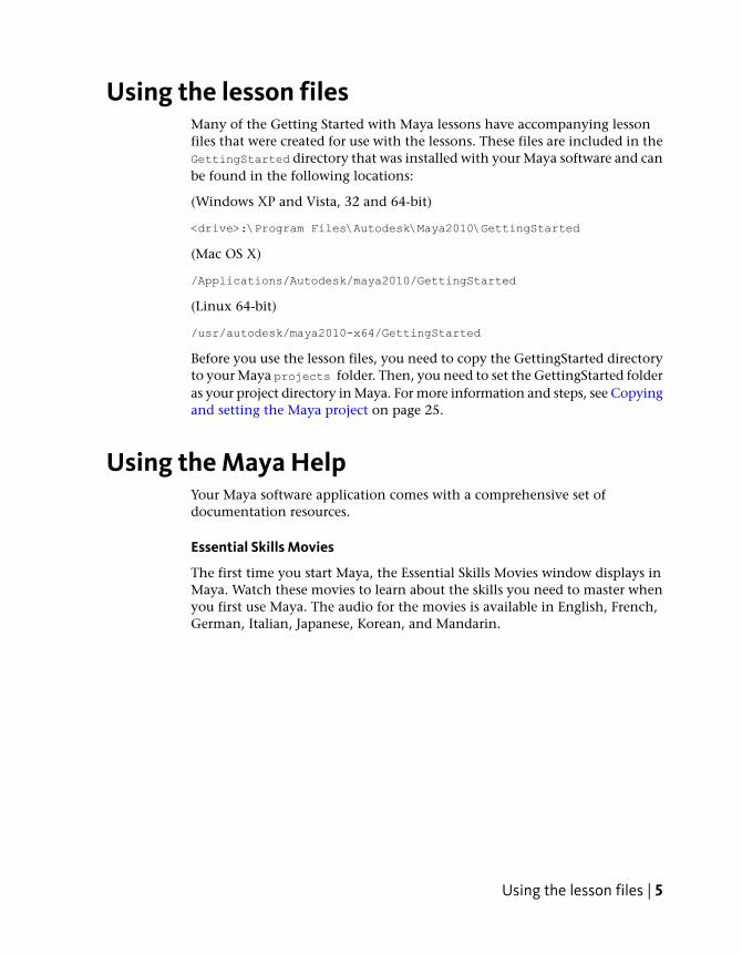
Using the lesson filesMany of the Getting Started with Maya lessons have accompanying lessonfiles that were created for use with the lessons. These files are included in theGettingStarted directory that was installed with your Maya software and canbe found in the following locations:
(Windows XP and Vista, 32 and 64-bit)
<drive>:\Program Files\Autodesk\Maya2010\GettingStarted
(Mac OS X)
/Applications/Autodesk/maya2010/GettingStarted
(Linux 64-bit)
/usr/autodesk/maya2010-x64/GettingStarted
Before you use the lesson files, you need to copy the GettingStarted directoryto your Maya projects folder. Then, you need to set the GettingStarted folderas your project directory in Maya. For more information and steps, see Copyingand setting the Maya project on page 25.
Using the Maya HelpYour Maya software application comes with a comprehensive set ofdocumentation resources.
Essential Skills Movies
The first time you start Maya, the Essential Skills Movies window displays inMaya. Watch these movies to learn about the skills you need to master whenyou first use Maya. The audio for the movies is available in English, French,German, Italian, Japanese, Korean, and Mandarin.
Using the lesson files | 5

To play the Essential Skills Movies
1 In the Essential Skills Movies window, click the buttons to play a movie.
Your computer launches the necessary multimedia player and your chosenmovie begins to play.
2 Click your multimedia player’s controls to start, stop, and pause themovie.
To close the Essential Skills Movies window or the multimedia player
1 To close the Essential Skills Movies window, click the close box in theupper right corner of the window.
If you do not want to have this dialog box automatically display whenyou start Maya, turn on the Don’t show this at startup check box.
2 To close the multimedia player, select File > Exit or click the close box inthe upper right corner of the window. (This instruction might varydepending upon which multimedia player is used)
If you want to watch the movies in the future
➤ In Maya, select Help > Learning Movies.
The Learning Movies window appears.
6 | Chapter 1 Overview

Maya Help
Your Maya software application comes installed with Maya technicaldocumentation that assists you in learning the Maya software. The Maya Helpis HTML-based, structured by module, fully searchable, and is displayed usingyour computer’s web browser.
The Maya Help is topic based and displays the major functionality categoriesfor Maya. The Maya Help can assist you in finding reference information aboutparticular topics, how to perform specific tasks, and MELTM commandreferences.
To launch the Maya Help
➤ Select Help > Maya Help.
The Maya Help appears in a separate web browser window (dependingon your user preference settings). The left hand pane of the Maya Helplets you navigate to various Maya topics.
To obtain help on a particular Maya topic
➤ In the Maya Help navigation pane, click the name of the Maya topic youwant information about (for example, Modeling, Animation, Dynamics,MEL commands, and so on).
The Maya Help displays the associated sub-topics and categories associatedwith the name you selected.
Maya Index and search
You can search the Maya Help directly using the index and search capabilities.With these tools you find the Maya topic you’re looking for by searching thetopic word in an alphabetic list or by directly typing the topic word(s) intothe search field and having the search tool find the documentation entriesassociated with it.
To use the Maya Index
1 In Maya, select Help > Maya Help.
The Maya Help appears in a separate window (depending on your userpreferences). The Maya Index button appears at the top of the leftnavigation pane.
2 Click the Index button.
Using the Maya Help | 7

The navigation pane updates to display an alphabetic list at the top ofthe pane with the first index items listed.
3 Click an item/letter in the alphabetic list.
The information related to that topic appears in the right pane.
To use the Maya Help search
1 Select Help > Maya Help.
The Maya Help appears in a separate window (depending on your userpreferences). The Maya Search button appears at the top of the leftnavigation pane.
2 Click the Search button.
The navigation pane updates to display the available search methods andoptions. You search a topic by typing in a word(s) that best represent theinformation you require.
3 In the text box, type a word that best represents your search topic.
By default, all of the content in the Maya Help is searched. You cannarrow the search results by selecting a specific user guide from the dropdown list below the text box.
4 Click the Search button to begin.
The search results appear in the left navigation pane, in order of relevancy.
5 Click the desired topic from the search results list.
The information related to that entry appears in the right pane of theMaya Help.
Popup Help
Popup Help provides you with a quick method of identifying a particular toolor icon in the Maya user interface.
8 | Chapter 1 Overview

To use Popup Help
➤ Move your mouse cursor over an icon or button.
The name or description of it appears in a popup window directly overit.
To turn on the Popup Help if it does not appear
1 If you’re operating Maya on a Windows or Linux operating system:
■ Select Window > Settings/Preferences > Preferences.
■ In the Preferences window, click the Help category and set the Tooltipsbox to Enable in the Popup Help section so a check mark appears.
■ Click the Save button to close the Preferences window.
2 If you’re operating Maya on a Mac OS X operating system:
■ Select Maya > Preferences.
■ In the Preferences window, click the Help category and click theTooltips Enable box in the Popup Help section so a check markappears.
■ Click the Save button to close the Preferences window.
Help Line
The Help Line at the bottom of Maya's window shows information abouttools, menus, and objects. Like the Popup help, it displays descriptions whenyou move the mouse over icons and menu items. It also displays instructionswhen you select a tool. This is useful if you don’t know or forget how to usea particular tool.
Using the Maya Help | 9
To use the Help Line
➤ Move your mouse cursor over an icon or button.
The icon or button name and instructions about how to use that toolappear in the Help Line.
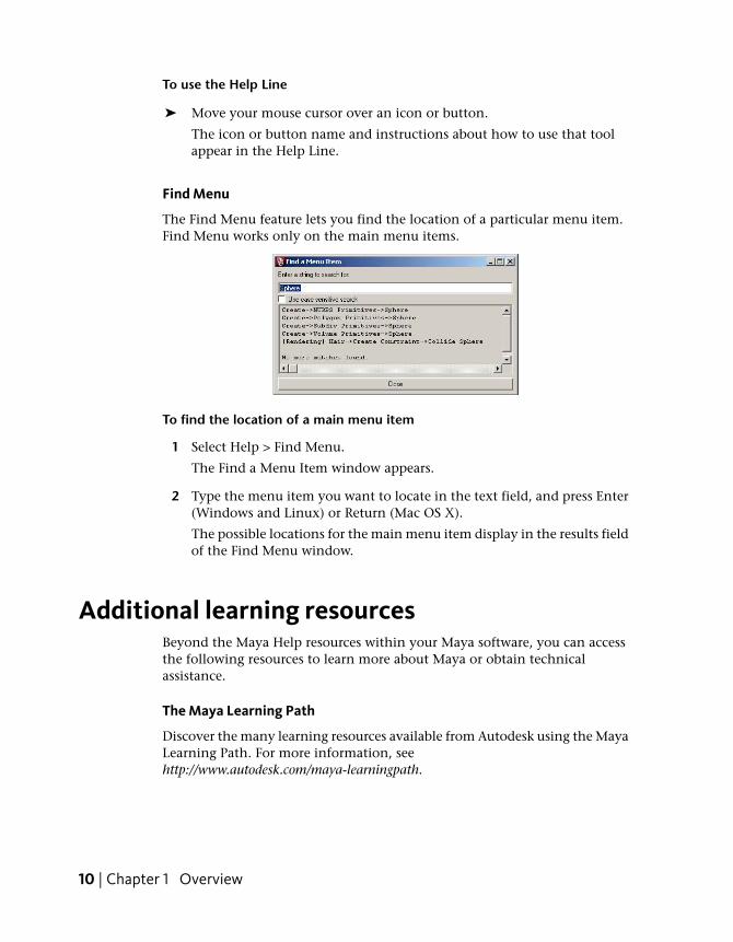
Find Menu
The Find Menu feature lets you find the location of a particular menu item.Find Menu works only on the main menu items.
To find the location of a main menu item
1 Select Help > Find Menu.
The Find a Menu Item window appears.
2 Type the menu item you want to locate in the text field, and press Enter(Windows and Linux) or Return (Mac OS X).
The possible locations for the main menu item display in the results fieldof the Find Menu window.
Additional learning resourcesBeyond the Maya Help resources within your Maya software, you can accessthe following resources to learn more about Maya or obtain technicalassistance.
The Maya Learning Path
Discover the many learning resources available from Autodesk using the MayaLearning Path. For more information, seehttp://www.autodesk.com/maya-learningpath.
10 | Chapter 1 Overview
The Maya Web site
The Maya Web site contains a wealth of resources related to your Maya softwareand many other related products and services. You can view the Maya Website athttp://www.autodesk.com/maya using your web browser.
Autodesk Training
Autodesk provides a range of products and services to help you get the mostfrom your Maya software. You can purchase additional self-paced learningmaterials or attend certified instructor led training courses at Autodesksanctioned training facilities. For more information, seehttp://www.autodesk.com/maya-training.
Technical Support
Autodesk delivers technical support services for Maya globally throughtelephone and email services, as well as online eSupport services. For moreinformation, click the Support Center link from the Maya Help menu or clickthe Services and Support link on the Maya Web site.
Events and Seminars
Autodesk also runs Maya seminars and short format training courses at majorcomputing events and trade shows. For more information, seehttp://www.autodesk.com/maya-events-seminars.
Restoring default user settingsIf you have already used Maya or have a prior version of Maya installed, youshould restore the default settings for Maya before you begin the lessons. Thisensures that Maya appears and operates exactly as the lessons describe.
If you are an existing user of Maya we recommend that you save your existingpreferences for later use prior to restoring the default user settings.
To save your existing custom user preferences
1 Ensure Maya is not running.
Each time you exit Maya it saves the configuration of most componentsof your user interface so it appears the same when you start it the nexttime. It writes the preferences to a directory called prefs. If you renamethe prefs directory, your original preferences will be maintained and Mayawill create a new prefs directory the next time it is run.
Restoring default user settings | 11
2 Rename your existing user preferences file to a different name; forexample, myprefs. The prefs directory path is:
Windows
(Windows XP)
\Documents and Settings\<username>\My Documents\maya\
2010\en_US\prefs
(Windows XP 64bit)
\Documents and Settings\<username>\My Documents\maya\ 2010-
x64\en_US\prefs
(Windows Vista)
\Users\<username>\Documents\maya\2010\en_US\prefs
(Windows Vista 64-bit)
\Users\<username>\Documents\maya\2010-x64\en_US\prefs
Mac OS X
/Users/<username>/Library/Prefer
ences/Autodesk/maya/en_US/2010/prefs
Linux (64-bit)
~<username>/maya/2010-x64/prefs
NOTE If you are running the Japanese version of Maya, change en_US in theabove directory paths to ja_JP.
If you have a previous version of Maya installed, also rename that prefsdirectory to a new name such as myprefs. Maya will load older preferencesif they exist from a previous version.
3 Start Maya and begin the Getting Started with Maya lessons.
To restore your custom user preferences after doing the lessons
1 Ensure Maya is not running.
2 Rename the previously changed preferences back to prefs.
12 | Chapter 1 Overview
Maya Basics
Introduction
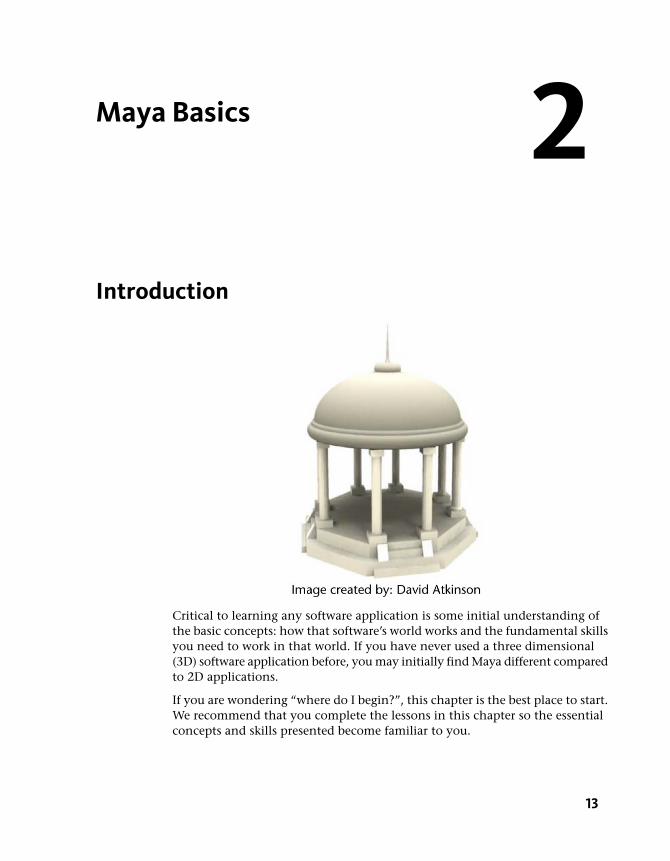
Critical to learning any software application is some initial understanding ofthe basic concepts: how that software’s world works and the fundamental skillsyou need to work in that world. If you have never used a three dimensional(3D) software application before, you may initially find Maya different comparedto 2D applications.
If you are wondering “where do I begin?”, this chapter is the best place to start.We recommend that you complete the lessons in this chapter so the essentialconcepts and skills presented become familiar to you.
2
13

This chapter covers some of the fundamental concepts and skills for Maya infour lessons:
■ Lesson 1 The Maya user interface: Introduction on page 15
■ Lesson 2 Creating, manipulating, and viewing objects: Introduction onpage 29
■ Lesson 3 Viewing the Maya 3D scene: Introduction on page 42
■ Lesson 4 Components and attributes: Introduction on page 60
Preparing for the lessonsTo ensure the lessons work as described:
■ Ensure Maya is installed and licensed on your computer.If you have not installed Maya yet, refer to the Installation and Licensingmanual that accompanies your Maya software package. It outlines therequirements for installing Maya and procedures for installation andlicensing Maya on supported hardware platforms.
■ If you have never started Maya on your computer before, it will start forthe first time using the default preference settings.
■ If you have run Maya before, you should ensure that your Maya userpreferences are reset to their default setting. This ensures that the lessonsappear and work as described.Refer to Restoring default user settings on page 11 for instructions onresetting user preferences to the default setting.
■ Unless otherwise indicated, the directions in this chapter for making menuselections assume you’re working from the Polygons menu set.
NOTE Before you perform the lessons in this book, ensure that the InteractiveCreation option for primitives is turned off by selecting Create > PolygonPrimitives > Interactive Creation and Create > NURBS Primitives > InteractiveCreation. That is, ensure a check mark does not appear beside these menuitems.
14 | Chapter 2 Maya Basics

Lesson 1: The Maya user interface
IntroductionJust as the driver of an automobile is familiar with the dashboard of theirvehicle, it is important for you to become familiar with the Maya “dashboard.”
The Maya user interface refers to everything that the Maya user sees and operateswithin Maya. The menus, icons, scene views, windows, and panels comprisethe user interface.
Through the Maya user interface you access the features and operate the toolsand editors that allow you to create, animate, and render your threedimensional objects, scenes, and effects within Maya.
As you spend time learning and working with Maya, your knowledge of andfamiliarity with the user interface will increase until it becomes second nature.
In this lesson you learn how to:
■ Start Maya on your computer.
■ Use the Maya interface so that you can begin to understand where andhow to access the critical tools to get started with Maya.
■ Select the menu and icon sets within Maya.
■ Learn the names of tools related to the icons in Maya.
■ Create a new scene view.
This first lesson contains additional explanations of the tools and conceptscompared to many of the lessons later in this manual. We suggest you takesome time to review these explanations as they lay the foundation forunderstanding where things are in Maya.
Starting Maya
To start Maya on Windows
➤ Do one of the following:
■ Double-click the Maya icon on your desktop.
Lesson 1: The Maya user interface | 15

■ From the Windows Start menu, select All Programs > Autodesk >Autodesk Maya 2010 > Maya 2010.
To start Maya on Mac OS X
➤ Do one of the following:
■ Double-click the Maya icon on your desktop.
■ Click the Maya icon in the Dock.
■ From the Apple Finder menu, select Go > Applications and then browsefor the Maya icon and double-click it to start Maya.
To start Maya on Linux
➤ Do one of the following:
■ Double-click the Maya icon on your desktop.
■ In a shell window, type: maya.
The Maya interfaceNow that Maya is running, you first need to understand what you are seeing.There are a lot of items displayed in the Maya user interface.
The best way to begin is to learn the fundamental tools and then learnadditional tools as you need them. Begin by learning some of the main tools.
16 | Chapter 2 Maya Basics

The Maya workspace
The Maya workspace is where you conduct most of your work within Maya.The workspace is the central window where your objects and most editorpanels appear.
The Maya interface | 17
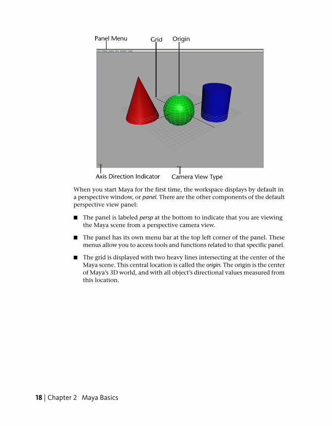
When you start Maya for the first time, the workspace displays by default ina perspective window, or panel. There are the other components of the defaultperspective view panel:
■ The panel is labeled persp at the bottom to indicate that you are viewingthe Maya scene from a perspective camera view.
■ The panel has its own menu bar at the top left corner of the panel. Thesemenus allow you to access tools and functions related to that specific panel.
■ The grid is displayed with two heavy lines intersecting at the center of theMaya scene. This central location is called the origin. The origin is the centerof Maya’s 3D world, and with all object’s directional values measured fromthis location.
18 | Chapter 2 Maya Basics
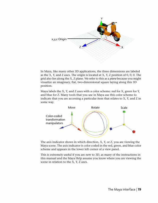
In Maya, like many other 3D applications, the three dimensions are labeledas the X, Y, and Z axes. The origin is located at X, Y, Z position of 0, 0, 0. Thegrid also lies along the X, Z plane. We refer to this as a plane because you mightvisualize an imaginary, flat, two-dimensional square laying along this 3Dposition.
Maya labels the X, Y, and Z axes with a color scheme: red for X, green for Y,and blue for Z. Many tools that you use in Maya use this color scheme toindicate that you are accessing a particular item that relates to X, Y, and Z insome way.
The axis indicator shows in which direction, X, Y, or Z, you are viewing theMaya scene. The axis indicator is color coded in the red, green, and blue colorscheme and appears in the lower left corner of a view panel.
This is extremely useful if you are new to 3D, as many of the instructions inthis manual and the Maya Help assume you know where you are viewing thescene in relation to the X, Y, Z axes.
The Maya interface | 19

Main Menu bar
Tools and items are accessible from pull down menus located at the top ofthe user interface. In Maya, menus are grouped into menu sets. These menusets are accessible from the Main Menu bar.
The Main Menu bar appears at the top of the Maya interface directly belowthe Maya title bar and displays the chosen menu set. Each menu setcorresponds to a module within Maya: Animation, Polygons, Surfaces,Rendering, and Dynamics. Modules are a method for grouping related featuresand tools.
You switch between menu sets by choosing the appropriate module from themenu selector on the Status Line (located directly below the File and Editmenus). As you switch between menu sets, the right-hand portion of themenus change, but the left-hand portion remains the same; the left-handmenus are common menus to all menu sets. The left-hand menus containFile, Edit, Modify, Create, Display, and Window.
To select a specific menu set
1 On the Status line, select Animation from the drop-down menu.
The Main Menu changes to display the menu set that relates to theAnimation module. In particular, menu titles such as Animate, Deform,Skeleton, Skin, and so on, appear.
2 Using the menu selector, choose Polygons from the drop-down menu.
20 | Chapter 2 Maya Basics

The main menu changes to display the menu set for Polygons. Menutitles such as Select, Mesh, Edit Mesh, and so on, appear.
For now, leave the menu set at Polygons. You will use this set in the nextstep.
To create a primitive 3D object from the Polygons menu set
1 Select Create > Polygon Primitives > Interactive Creation and ensure thata check mark does not appear beside this item.
For this lesson, you won’t use this option.
2 From the Main Menu Bar, select Create > Polygon Primitives > Cube >.
Maya creates a 3D cube primitive object and places it at the center (origin)of the Maya workspace.
Status Line
The Status Line, located directly below the Main Menu bar, contains a varietyof items, most of which are used while modeling or working with objectswithin Maya. Many of the Status Line items are represented by a graphicalicon. The icons save space in the Maya interface and allow for quick access totools used most often.
In this lesson, you learn about some of the Status Line areas.
You’ve already learned the first item on the Status line: the Menu Selectorused to select between menu sets.
The Maya interface | 21
The second group of circled icons relate to the scene and are used to create,open, and save your Maya scenes.
The third and fourth group of buttons are used to control how you can selectobjects and components of objects. You will learn more about selection ofobjects in later lessons.
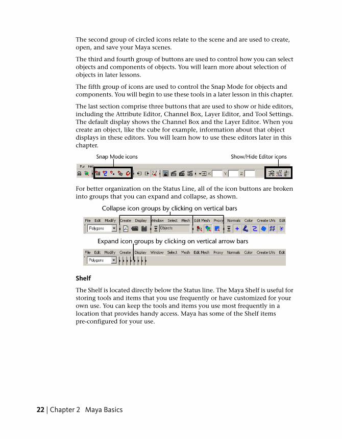
The fifth group of icons are used to control the Snap Mode for objects andcomponents. You will begin to use these tools in a later lesson in this chapter.
The last section comprise three buttons that are used to show or hide editors,including the Attribute Editor, Channel Box, Layer Editor, and Tool Settings.The default display shows the Channel Box and the Layer Editor. When youcreate an object, like the cube for example, information about that objectdisplays in these editors. You will learn how to use these editors later in thischapter.
For better organization on the Status Line, all of the icon buttons are brokeninto groups that you can expand and collapse, as shown.
Shelf
The Shelf is located directly below the Status line. The Maya Shelf is useful forstoring tools and items that you use frequently or have customized for yourown use. You can keep the tools and items you use most frequently in alocation that provides handy access. Maya has some of the Shelf itemspre-configured for your use.
22 | Chapter 2 Maya Basics

To create an object using a tool from the Shelf
1 From the Shelf, select the Surfaces tab in order to view the tools locatedon that shelf.
2 Select Create > NURBS Primitives > Interactive Creation to ensure that acheck mark does not appear beside the item.
For this lesson, you won’t use this option
3 From the Shelf, select the NURBS sphere icon located at the left end byclicking on it.
Maya creates a sphere primitive object and places it at the center of theMaya workspace in the same position as the cube.
TIP You can determine if this is the correct tool prior to choosing it by firstplacing your mouse cursor over the icon, the name or description of it appearsin a popup window directly over it.
The Maya interface | 23

In your scene view the wireframe outline of the cube you created earlier inthe lesson has changed color to navy blue, and the sphere is displayed in abright green color. The sphere is now the selected object and the cube is nolonger selected. In Maya, when the object displays like this, we refer to it asbeing selected or active.
Selection of objects and components is a way of indicating to Maya that thisparticular item is to be affected by the tool or action you will subsequentlychoose. As you work with Maya, you will be selecting and deselecting itemsa lot. You will learn how to select and deselect objects later in this chapter.
Some numerical information appears in the Channel Box editor on the righthand side of the user interface. This information relates to X, Y, and Z,translation, rotation, and scaling for the active object. The X, Y, and Z Translatenumerical values are currently set to 0. This indicates that the sphere’s locationis at the origin. The Channel Box is useful for viewing and editing this typeof basic information. You will use the Channel Box later in this chapter.
24 | Chapter 2 Maya Basics

To hide or show the Channel Box
1 To hide the Channel Box, click the Show/Hide Channel Box icon fromthe right end of the Status line.
The Channel Box disappears, and the perspective scene view expandsslightly. With the Channel Box hidden, you have more working area inyour scene view.
2 To show the Channel Box, click the Show/Hide Channel Box icon onthe Status line. The Channel Box appears in the scene view.
Copying and setting the Maya projectBefore you can save your work, you need to set a project in Maya.
A project is a file directory that stores and organizes all of the files (scenes,images, materials, textures, etc.) related to a particular scene. In Maya, youcreate and work with a variety of file types and formats. The project directoryallows you to keep these different file types in their unique subdirectorylocations within the project directory.
You can create a new project directory by choosing File > Project > New.Alternatively, you can choose an existing folder to act as the project directoryif you have prepared a folder in advance.
For these lessons, the project directory will be the GettingStarted folder thatwe have created for you. Here, you will find all the template files that youneed for the lessons, and you will save your work as you learn. You need tocopy the GettingStarted folder to your Maya projects folder, and then youneed to set the GettingStarted folder as the project directory in Maya.
To copy and set the GettingStarted folder as your Maya project
1 Navigate to the GettingStarted folder that was installed with your Mayasoftware. The location of this folder depends on the operating systemthat you are using.
Copying and setting the Maya project | 25

(Windows XP and Vista, 32 or 64-bit)
<drive>:\Program Files\Autodesk\Maya2010\GettingStarted
(Mac OS X)
/Applications/Autodesk/maya2010/GettingStarted
(Linux 64-bit)
/usr/autodesk/maya2010-x64/GettingStarted
2 Copy the GettingStarted folder.
3 Paste the GettingStarted folder in one of the following locations,depending on the operating system that you are using:
(Windows XP, 32 or 64-bit)
<drive>:\Documents and Settings\<username>\My Documents\maya\pro
jects
(Windows Vista, 32 or 64-bit)
<drive>:\Users\<username>\My Documents\maya\projects
(Mac OS X)
/Users/<username>/Documents/maya/projects
(Linux 64-bit)
<home directory>/maya/projects
4 In Maya, choose File > Project > Set.
5 Browse for the GettingStarted folder that you pasted in your Mayaprojects directory in step 3.
6 Select the folder and click OK.
Saving your workMake it a habit to save your work often when working on your Maya projects.In that way, you can always open an earlier version of your work should youmake a mistake.
Maya refers to everything you’ve created in your workspace as the scene. Thisincludes any objects, lights, cameras and materials associated with yourworking session.
26 | Chapter 2 Maya Basics

To save your Maya scene
1 Select File > Save Scene.
A file browser appears, listing the GettingStarted project directory whereyou can save your scene.
If the GettingStarted directory does not appear, you need to copy theGettingStarted folder and set it as your Maya project. See Copying andsetting the Maya project on page 25.
2 Within the GettingStarted directory, double-click the scenes folder toopen it.
3 Type: Lesson1 in the file name text box.
4 Click Save.
Maya saves your file to the scenes directory within your GettingStartedproject directory. Maya automatically saves the file with a .mb fileextension. The .mb file extension indicates that the scene was saved as aMaya binary file: the default file type for a Maya scene.
Exiting MayaBefore you exit Maya, ensure you save any work that you want to retrieve andcontinue with at a later time.
To exit Maya
➤ Select File > Exit from the main menu.
Maya does one of the two following actions:
■ If you have saved your scene immediately preceding the Exit command,Maya exits.
■ If you have not recently saved your scene, a message prompt appears onthe screen asking if you want to save your changes. Click either Save, Don’tSave, or Cancel.
Exiting Maya | 27

Beyond the lessonIn this lesson you began your orientation to Maya by learning:
■ How to start Maya on your computer.
■ The Maya workspace, and how it shows three dimensional space (X, Y, Z).
■ How Maya color-codes items and tools related to X, Y, Z.
■ The location of the main menus for the various modules within Maya.
■ How to create a three-dimensional object from the Polygons menu.
■ The location of the Status Line and how items are displayed as icons.
■ About the Shelf how to create a three dimensional object from the Shelf.
■ How to hide and show the Channel Box and that basic transformation,scaling, and rotational information for an object can viewed in the ChannelBox.
■ How to save your work.
■ How to exit Maya.
As you proceed through Getting Started with Maya you should be familiarwith the fundamental concepts and skills covered in this first chapter.
If you want to learn more about a particular tool or feature that has beenpresented in this lesson, refer to the Maya Help.
28 | Chapter 2 Maya Basics

Lesson 2: Creating, manipulating, and viewingobjects
Introduction
Using primitive objects to model 3D forms is a great place to continue learningabout Maya. You can create many types of 3D objects using Maya and thenmove, scale, and rotate them to create more complex forms in your scene.
In this lesson, you begin to construct a classic temple using the primitiveobject creation tools in Maya. The project is not very complex and providesyou with experience in using some of the important object manipulation andviewing tools.
As you continue to work with Maya, you’ll learn how to visualize morecomplex forms using these basic objects. Maya has many advanced tools andoptions for modeling complex forms, as you will learn in later chapters.
In this lesson, you learn how to:
■ Create 3D primitive objects.
■ Select objects for manipulation and editing purposes.
■ Move and rotate objects using your mouse.
■ Move, rotate, and scale objects using numeric input.
■ Duplicate objects.
■ Change the viewing panels in Maya using a variety of methods so you canview your objects from different points of view.
■ Undo actions when you need to undo a particular task or step.
Lesson 2: Creating, manipulating, and viewing objects | 29

Creating a new sceneYou begin your temple project by creating a new empty scene.
To create a new scene
1 Start Maya (if it is not already running).
When Maya starts, it automatically creates a new scene.
If Maya was previously running, follow steps 2 and 3.
2 From the main menu, select File > New Scene.
Maya displays the following prompt.
3 Click No.
Maya creates a new scene and delete everything that was in the previousscene.
Primitive objectsMaya provides many types of primitive types and shapes such cubes, spheres,cylinders, and planes.
Primitive objects can be used as a starting point for a wide variety of shapesand forms. The most common workflow when using primitive objects is:
■ Set the construction options for the primitive when you initially create itso that it appears in the Maya scene roughly in the size and shape thatyou require.
■ Move, scale, and rotate the primitive object into its final position eitherby direct manipulation (the move, scale, and rotate tools), or by enteringnumeric values through an editor.
30 | Chapter 2 Maya Basics

■ Duplicate the primitive objects to create multiple copies of the original orcreate different variations from your original primitive object.
In this section, you construct the base for the temple using a polygonal cylinderprimitive. The octagonal shape is created by modifying the creation optionsfor the cylinder tool before you create the object. If you did not modify thecylinder options you would create a round cylinder.
To create a polygonal cylinder for the base
1 Select the Polygons menu set.
NOTE Unless otherwise indicated, the directions in this lesson for makingmenu selections assume you’ve already selected the Polygons menu set.
You should also ensure that the Interactive Creation option for primitives isfirst turned off by selecting Create > Polygon Primitives > Interactive Creationto ensure the check mark does not appear beside the item.
2 From the main menu, select Create > Polygon Primitives > Cylinder >.
An option window appears.
3 In the Polygon Cylinder Options window, select Edit > Reset Settings andthen set the following options:
■ Radius: 10
■ Height: 1
■ Axis divisions: 8
■ Height divisions: 1
■ Cap divisions: 1
■ Axis: Y
4 In the Polygon Cylinder Options window, click Create.
Maya creates a cylinder primitive object that is octagonal in shape andpositioned at the center of the Maya workspace. This cylinder is 20 unitswide by one unit high, and has eight faceted sides.
Primitive objects | 31
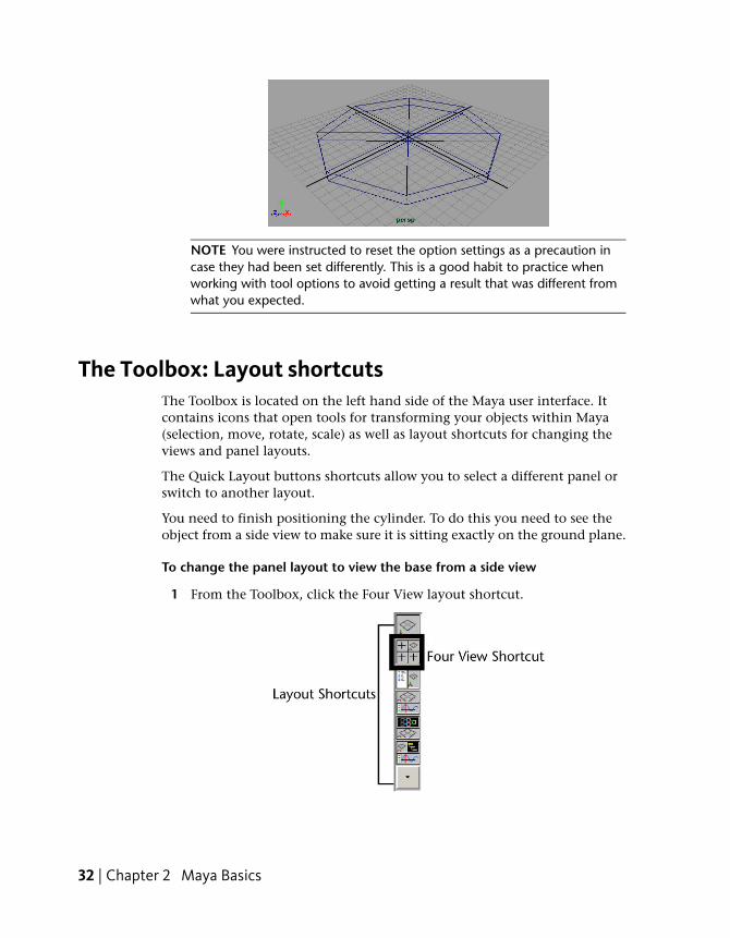
NOTE You were instructed to reset the option settings as a precaution incase they had been set differently. This is a good habit to practice whenworking with tool options to avoid getting a result that was different fromwhat you expected.
The Toolbox: Layout shortcutsThe Toolbox is located on the left hand side of the Maya user interface. Itcontains icons that open tools for transforming your objects within Maya(selection, move, rotate, scale) as well as layout shortcuts for changing theviews and panel layouts.
The Quick Layout buttons shortcuts allow you to select a different panel orswitch to another layout.
You need to finish positioning the cylinder. To do this you need to see theobject from a side view to make sure it is sitting exactly on the ground plane.
To change the panel layout to view the base from a side view
1 From the Toolbox, click the Four View layout shortcut.
32 | Chapter 2 Maya Basics
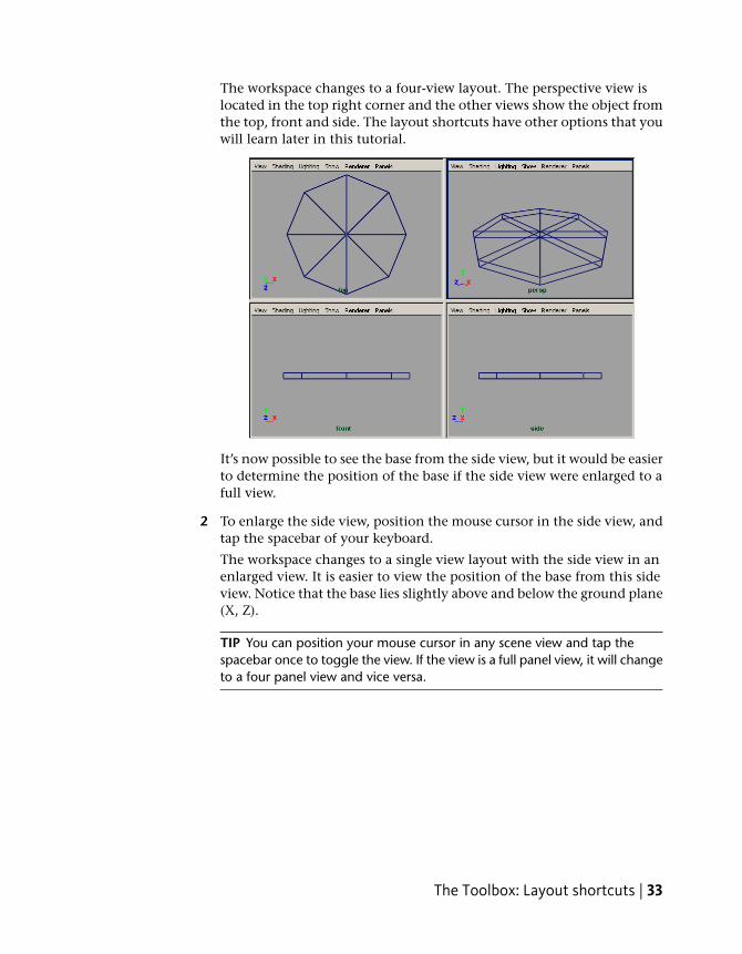
The workspace changes to a four-view layout. The perspective view islocated in the top right corner and the other views show the object fromthe top, front and side. The layout shortcuts have other options that youwill learn later in this tutorial.
It’s now possible to see the base from the side view, but it would be easierto determine the position of the base if the side view were enlarged to afull view.
2 To enlarge the side view, position the mouse cursor in the side view, andtap the spacebar of your keyboard.
The workspace changes to a single view layout with the side view in anenlarged view. It is easier to view the position of the base from this sideview. Notice that the base lies slightly above and below the ground plane(X, Z).
TIP You can position your mouse cursor in any scene view and tap thespacebar once to toggle the view. If the view is a full panel view, it will changeto a four panel view and vice versa.
The Toolbox: Layout shortcuts | 33

The Toolbox: Transformation toolsYou need to move the base slightly upwards in the Y direction so it ispositioned on the X, Z plane. To do this you use the Move transformationtool located in the Toolbox.
The upper half of the Toolbox contains the tools for transforming objects(selection, move, rotate, scale) within Maya. When you move your mousecursor over any transformation tool icon you see the name of the tool appearnext to the mouse cursor.
The tool’s name also appears in the Help Line at the bottom of the Mayawindow. The Help Line has an additional purpose: it displays summaryinstructions as you use tools that require several steps.
Selection and de-selection of objects
Before you can transform an object, you must ensure it is selected. You canselect objects by clicking them directly, or by dragging a rectangular boundingbox around some portion of the object to indicate what you want selected.To deselect an object, you simply click somewhere off of the selected object.
34 | Chapter 2 Maya Basics
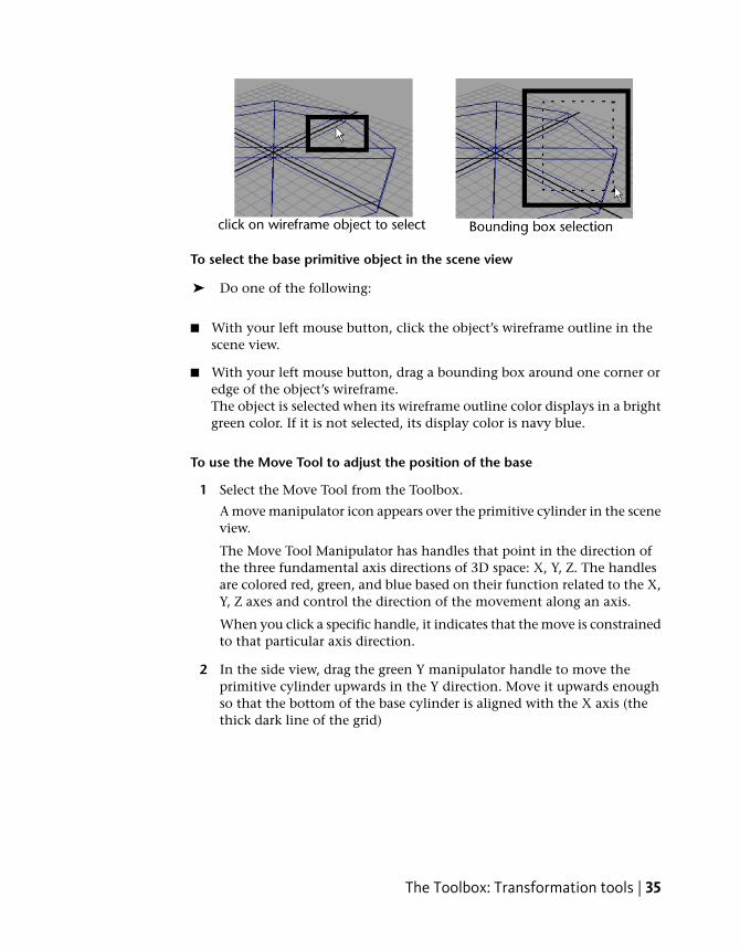
To select the base primitive object in the scene view
➤ Do one of the following:
■ With your left mouse button, click the object’s wireframe outline in thescene view.
■ With your left mouse button, drag a bounding box around one corner oredge of the object’s wireframe.The object is selected when its wireframe outline color displays in a brightgreen color. If it is not selected, its display color is navy blue.
To use the Move Tool to adjust the position of the base
1 Select the Move Tool from the Toolbox.
A move manipulator icon appears over the primitive cylinder in the sceneview.
The Move Tool Manipulator has handles that point in the direction ofthe three fundamental axis directions of 3D space: X, Y, Z. The handlesare colored red, green, and blue based on their function related to the X,Y, Z axes and control the direction of the movement along an axis.
When you click a specific handle, it indicates that the move is constrainedto that particular axis direction.
2 In the side view, drag the green Y manipulator handle to move theprimitive cylinder upwards in the Y direction. Move it upwards enoughso that the bottom of the base cylinder is aligned with the X axis (thethick dark line of the grid)
The Toolbox: Transformation tools | 35
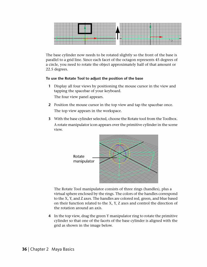
The base cylinder now needs to be rotated slightly so the front of the base isparallel to a grid line. Since each facet of the octagon represents 45 degrees ofa circle, you need to rotate the object approximately half of that amount or22.5 degrees.
To use the Rotate Tool to adjust the position of the base
1 Display all four views by positioning the mouse cursor in the view andtapping the spacebar of your keyboard.
The four view panel appears.
2 Position the mouse cursor in the top view and tap the spacebar once.
The top view appears in the workspace.
3 With the base cylinder selected, choose the Rotate tool from the Toolbox.
A rotate manipulator icon appears over the primitive cylinder in the sceneview.
The Rotate Tool manipulator consists of three rings (handles), plus avirtual sphere enclosed by the rings. The colors of the handles correspondto the X, Y, and Z axes. The handles are colored red, green, and blue basedon their function related to the X, Y, Z axes and control the direction ofthe rotation around an axis.
4 In the top view, drag the green Y manipulator ring to rotate the primitivecylinder so that one of the facets of the base cylinder is aligned with thegrid as shown in the image below.
36 | Chapter 2 Maya Basics
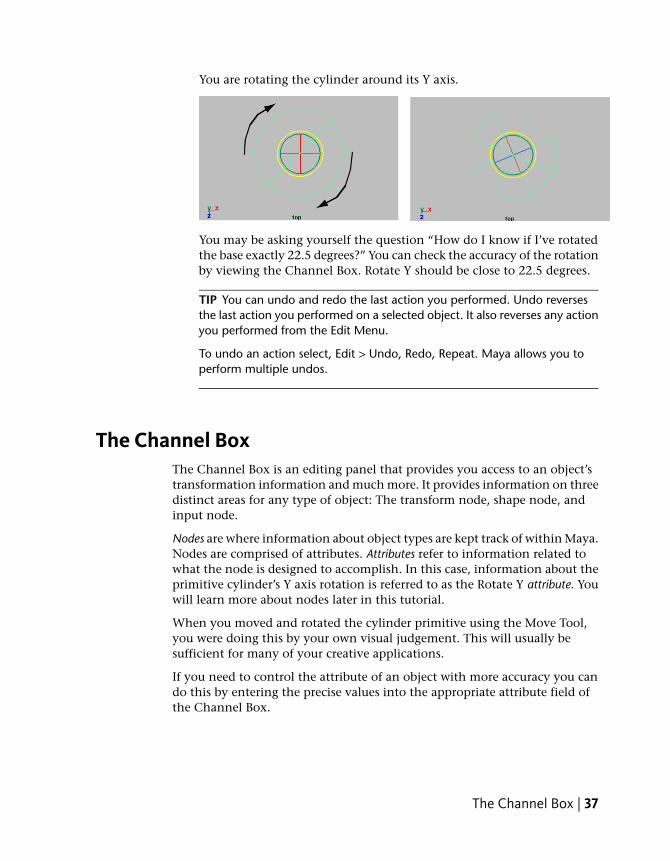
You are rotating the cylinder around its Y axis.
You may be asking yourself the question “How do I know if I’ve rotatedthe base exactly 22.5 degrees?” You can check the accuracy of the rotationby viewing the Channel Box. Rotate Y should be close to 22.5 degrees.
TIP You can undo and redo the last action you performed. Undo reversesthe last action you performed on a selected object. It also reverses any actionyou performed from the Edit Menu.
To undo an action select, Edit > Undo, Redo, Repeat. Maya allows you toperform multiple undos.
The Channel BoxThe Channel Box is an editing panel that provides you access to an object’stransformation information and much more. It provides information on threedistinct areas for any type of object: The transform node, shape node, andinput node.
Nodes are where information about object types are kept track of within Maya.Nodes are comprised of attributes. Attributes refer to information related towhat the node is designed to accomplish. In this case, information about theprimitive cylinder’s Y axis rotation is referred to as the Rotate Y attribute. Youwill learn more about nodes later in this tutorial.
When you moved and rotated the cylinder primitive using the Move Tool,you were doing this by your own visual judgement. This will usually besufficient for many of your creative applications.
If you need to control the attribute of an object with more accuracy you cando this by entering the precise values into the appropriate attribute field ofthe Channel Box.
The Channel Box | 37

To move and rotate the base using the Channel Box
1 With the base cylinder selected, view the Transformation attributes inthe Channel Box. Specifically, view the values for Translate Y, and RotateY.
2 In the Channel Box, adjust the attribute values so they match the aboveimage by clicking in the field and entering the correct numerical values.
This accurately positions the base in your Maya scene.
Maya named the cylinder primitive when it was first created. Renamethe cylinder to something more meaningful to your project.
To rename the cylinder primitive using the Channel Box
1 In the Channel Box, click in the field with the name pCylinder1.
2 Rename the primitive object by typing the new name: templeBase andthen pressing Enter.
38 | Chapter 2 Maya Basics
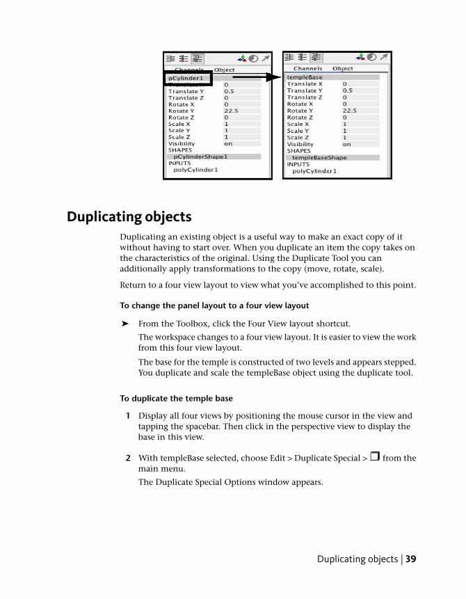
Duplicating objectsDuplicating an existing object is a useful way to make an exact copy of itwithout having to start over. When you duplicate an item the copy takes onthe characteristics of the original. Using the Duplicate Tool you canadditionally apply transformations to the copy (move, rotate, scale).
Return to a four view layout to view what you’ve accomplished to this point.
To change the panel layout to a four view layout
➤ From the Toolbox, click the Four View layout shortcut.
The workspace changes to a four view layout. It is easier to view the workfrom this four view layout.
The base for the temple is constructed of two levels and appears stepped.You duplicate and scale the templeBase object using the duplicate tool.
To duplicate the temple base
1 Display all four views by positioning the mouse cursor in the view andtapping the spacebar. Then click in the perspective view to display thebase in this view.
2 With templeBase selected, choose Edit > Duplicate Special > from themain menu.
The Duplicate Special Options window appears.
Duplicating objects | 39

3 In the Duplicate Special Options window, select Edit > Reset Settings andthen set the following options:
■ Translate: 0 1.0 0
■ Rotate: 0 0 0
■ Scale: 0.9 1.0 0.9
■ Geometry Type: Copy
■ Group under: Parent
4 In the Duplicate Options window, click Duplicate Special.
Maya creates a duplicate of the templeBase object that is scaled to 0.9 ofthe original in the X, Z axes, and is one unit above templeBase. As a resultof the scale operation, the base for the temple now appears stepped.
Maya keeps track of the name of the duplicated object based on the nameof original and renames the duplicated object templeBase1.
Save your workIn the last lesson we recommended that you save your work at regular intervals.An example of this is when you have just completed a major task such asconstructing the base for the temple. With this strategy, if you ever make amistake, you can always open the previously saved version of your work andbegin from there.
To save your Maya scene
1 Select File > Save Scene.
A file browser appears showing the GettingStarted project directorywhere you can save your scene.
40 | Chapter 2 Maya Basics

If you do not see the GettingStarted project directory, you have not yetcopied the GettingStarted folder and set it as your Maya project. Formore information, see Copying and setting the Maya project on page 25.
2 Within the GettingStarted project directory, ensure that you are savingin the scenes sub-directory.
3 Type Lesson2Base in the file name text box.
4 Click Save.
Beyond the lessonIn this lesson you continued with the fundamental tools and skills tosuccessfully learn:
■ An overall workflow for constructing forms using primitive objects.
■ Where the primitive object tools are located in the main menu.
■ How to create a primitive object as well as reset and edit its creationoptions.
■ How to change between a single view and four view panel layout usinglayout shortcuts and by tapping the spacebar of your keyboard.
■ How to select objects by clicking them with your mouse.
■ How to move and rotate objects using the transformation tools in theToolbox.
■ That tool manipulators can constrain a transformation to the X, Y, or Zaxes.
■ How to edit an object’s transformation node attributes (move, rotate, scale)accurately using the Channel Box.
■ How to rename objects using the Channel Box.
■ How to duplicate objects and apply transformations while doing so.
We suggest you additionally practice the following tasks on your own:
■ Creating other primitive object types, with various options so that youcan understand the variations that are possible.
Beyond the lesson | 41

■ Try using the ViewCube™ located in the upper-right corner of the activescene view to change the camera’s viewing angle in relation to the objectsin the scene.
■ Practice moving, rotating, and scaling objects, and changing between thevarious scene views (single perspective, four view, single side, single topetc.)
Lesson 3: Viewing the Maya 3D scene
Introduction
In the previous lesson you learned how to view your 3D scene by changingbetween single and four view layouts. It is important for you to learn how tochange your views in a more interactive manner so that you can: view yourobjects close up or far away, select objects more accurately, or view objectsfrom different angles in your perspective view.
In this lesson you learn how to:
■ Understand the difference between moving objects in the scene and movingthe point of view on the scene.
■ Use the dolly, track, and tumble camera tools to change the view of yourscene in both the orthographic and perspective views.
■ Rotate objects using the transformation tools in the Toolbox.
■ Select objects using a variety of techniques.
■ Group objects together so they can be transformed as a unit.
■ Display objects in both wireframe and shaded modes.
42 | Chapter 2 Maya Basics

■ Use additional primitive objects and options.
Camera toolsIn the lessons so far, when you looked at an object from the top, front, or sideviews you have been viewing the scene through an orthographic view.Orthographic views appear two-dimensional because the object is displayedusing parallel projections of only two axes at a time. (Scooter images courtesyof The Art of Maya)
When you view the scene through the perspective view, you are viewing thescene in a three-dimensional manner. The perspective view simulates whatyour scene would look like from a camera’s point of view.
In Maya, you view the scene through a set of virtual cameras. These camerasare either orthographic or perspective in nature. You can adjust how thesecameras view the scene using the Camera Tools.
The three primary methods for manipulating the camera view are dolly, tumble,and track.
Camera tools | 43

Dolly Tool
The Dolly Tool gets its name from filmmaking where a camera, mounted ona wheeled tripod, is moved towards or away from the scene. In Maya, dollyingallows you to view the items in your scene either close up or from furtherback.
To dolly the perspective view
1 Enlarge the scene view to a single perspective view.
2 Do one of the following:
■ (Windows & Linux) Press the Alt key and drag the mouse to the rightwhile holding down the right button on your mouse.
■ (Mac OS X) Press the Option key and drag the mouse to the rightwhile holding down the right button on your mouse.
3 To dolly the camera outwards from the subject in the scene you canperform the same key and mouse combinations as described above butdrag the mouse to the left.
Dolly works in both the perspective and orthographic views.
TIP If you make an error when adjusting your camera view of the scene, youcan reset the camera to its default home setting.
To reset the camera view for a particular orthographic or perspective view:
From the panel menu, select View > Default Home.
44 | Chapter 2 Maya Basics

Tumble Tool
The Tumble Tool allows you to tumble or rotate the camera’s view around aparticular center of interest to achieve either a higher or lower vantage point,or a different side angle.
To tumble the perspective view
➤ Press the Alt key (Windows & Linux) or the Option key (Mac OS X) anddrag the mouse either left or right, or up or down, while holding downthe left button on your mouse.
Tumbling the view revolves the camera around the center of the sceneview, in whichever direction you drag (left, right, up or down). TheTumble Tool does not work in the orthographic views.
Track Tool
The Track Tool allows you to move the camera up, down, or sideways inrelation to the scene.
Camera tools | 45
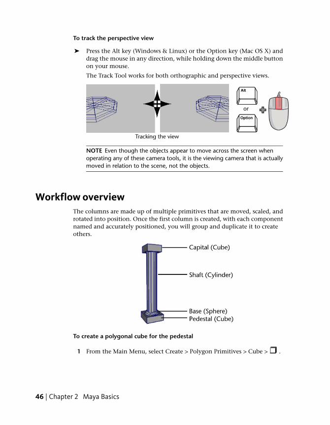
To track the perspective view
➤ Press the Alt key (Windows & Linux) or the Option key (Mac OS X) anddrag the mouse in any direction, while holding down the middle buttonon your mouse.
The Track Tool works for both orthographic and perspective views.
NOTE Even though the objects appear to move across the screen whenoperating any of these camera tools, it is the viewing camera that is actuallymoved in relation to the scene, not the objects.
Workflow overviewThe columns are made up of multiple primitives that are moved, scaled, androtated into position. Once the first column is created, with each componentnamed and accurately positioned, you will group and duplicate it to createothers.
To create a polygonal cube for the pedestal
1 From the Main Menu, select Create > Polygon Primitives > Cube > .
46 | Chapter 2 Maya Basics

2 In the Polygon Cube Options window, select Edit > Reset Settings andthen set the following options:
■ Width: 1.75
■ Height: 0.6
■ Depth: 1.75
Leave the other options at their default settings.
NOTE If the Polygon Cube Options window does not appear, ensure thatthe Interactive Creation option for primitives is turned off by first selectingCreate > Polygon Primitives > Interactive Creation so that a check mark doesnot appear beside this menu item.
3 In the Polygon Cube Options window, click Create.
Maya creates a cube primitive and positions it at the origin.
4 In the side view, move the cube upwards (Y axis) so it rests on the topsurface of the temple base.
You can do this using the Move Tool or with the Channel Box. If youuse the Channel Box, enter a Translate Y value of 2.3.
You may find it useful to dolly or tumble the scene view to obtain a betterviewpoint.
5 In the Channel Box, rename the cube columnPedestal.
To create a polygonal cylinder for the shaft
1 From the main menu, select Create > Polygon Primitives > Cylinder >.
Workflow overview | 47

2 In the Polygon Cylinder Options window, select Edit > Reset Settings andthen set the following options:
■ Radius: 0.5
■ Height: 6
■ Axis divisions: 12
Leave the other options at their default settings
3 In the Polygon Cylinder Options window, click Create.
Maya creates the cylinder primitive at the origin.
4 In side view, move the cylinder upwards (Y axis) so it rests on the topsurface of columnPedestal.
You can do this using the Move Tool or with the Channel Box. If youuse the Channel Box, enter a Translate Y value of 5.6.
5 In the Channel Box, rename the cylinder columnShaft.
The capital for the column rests on top of the column and is very similar tothe pedestal. You duplicate the pedestal and position the duplicate at the topof the column.
To duplicate the pedestal to create the capital
1 With only columnPedestal selected, select Edit > Duplicate Special >from the main menu.
The Duplicate Special Options window appears.
2 In the Duplicate Special Options window, select Edit > Reset Settings andthen set the following options:
■ Translate: 0 6.6 0
48 | Chapter 2 Maya Basics

■ Scale: 0.8 1.0 0.8
Leave the other options at their default settings.
3 In the Duplicate Special Options window, click Duplicate Special.
Maya creates a duplicate of the columnPedestal object and moves andscales it based on the options you set.
NOTE If you positioned the geometry for the column using the TransformTools and your mouse, the Y translate values may be incorrect for yourparticular model. You may want to continue positioning the objects by visualreference using your mouse.
Using the duplicate options is an alternate method for positioning andscaling duplicated objects when you can anticipate its final location.
4 In the Channel Box, rename the duplicated cube columnCapital.
The base for the column rests on top of the pedestal. You will create the baseusing one half of a NURBS sphere primitive and then move and rotate it intoposition. You will do this by modifying the creation options for the sphereprimitive.
To create a NURBS sphere for the column base
1 Select Create > NURBS Primitives > Sphere > .
2 In the NURBS Sphere Options window, select Edit > Reset Settings andthen set the following options:
■ Start Sweep Angle: 0
■ End Sweep Angle: 180
■ Radius: 0.75
Workflow overview | 49
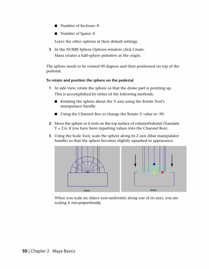
■ Number of Sections: 8
■ Number of Spans: 4
Leave the other options at their default settings.
3 In the NURBS Sphere Options window, click Create.
Maya creates a half-sphere primitive at the origin.
The sphere needs to be rotated 90 degrees and then positioned on top of thepedestal.
To rotate and position the sphere on the pedestal
1 In side view, rotate the sphere so that the dome part is pointing up.
This is accomplished by either of the following methods:
■ Rotating the sphere about the X axis using the Rotate Tool’smanipulator handle.
■ Using the Channel Box to change the Rotate X value to -90.
2 Move the sphere so it rests on the top surface of columnPedestal (TranslateY = 2.6, if you have been inputting values into the Channel Box).
3 Using the Scale Tool, scale the sphere along its Z axis (blue manipulatorhandle) so that the sphere becomes slightly squashed in appearance.
When you scale an object non-uniformly along one of its axes, you arescaling it non-proportionally.
50 | Chapter 2 Maya Basics
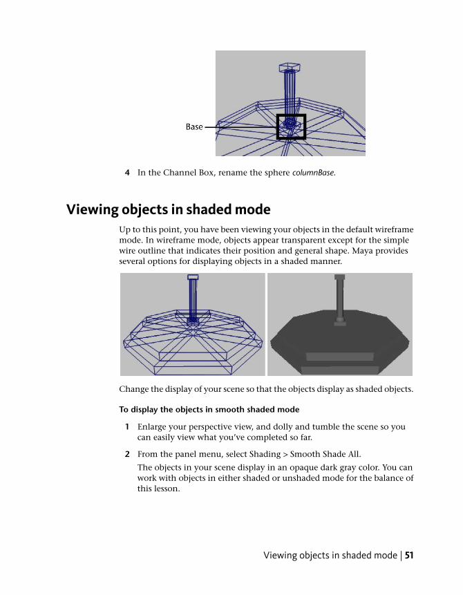
4 In the Channel Box, rename the sphere columnBase.
Viewing objects in shaded modeUp to this point, you have been viewing your objects in the default wireframemode. In wireframe mode, objects appear transparent except for the simplewire outline that indicates their position and general shape. Maya providesseveral options for displaying objects in a shaded manner.
Change the display of your scene so that the objects display as shaded objects.
To display the objects in smooth shaded mode
1 Enlarge your perspective view, and dolly and tumble the scene so youcan easily view what you’ve completed so far.
2 From the panel menu, select Shading > Smooth Shade All.
The objects in your scene display in an opaque dark gray color. You canwork with objects in either shaded or unshaded mode for the balance ofthis lesson.
Viewing objects in shaded mode | 51
Grouping objectsWhen you need to move, scale or rotate multiple objects as one unit it is easierif they have been grouped together so that they transform as one unit.
Many primitive objects in Maya are grouped objects. For example, the NURBScube primitive is comprised of 6 flat squares or planes that have been groupedtogether as one unit. When the plane objects are grouped together they createa hierarchy.
A hierarchy is a collection of nodes or objects that are connected together toform a unit for some purpose. Hierarchies are useful for describing how theobjects within them share similar characteristics or attributes; move, scale,rotate for example.
To group the objects for the column
1 Select the four objects that comprise the column simultaneously by doingone of the following:
■ With your left mouse button, shift-click each object in turn until thefour objects are selected in the scene view.
■ With your left mouse button, drag one large bounding box aroundthe column objects in an orthographic view.
It is important that you do not select any of the templeBase objects aspart of your selection. If you accidentally select any of the base objects,deselect them.
2 From the main menu, select Edit > Group > .
3 In the Group Options window, select Edit > Reset Settings and then setthe following options:
■ Group Under: Parent
Leave the other options at their default settings
4 In the Group Options window, click Group.
Maya groups the objects together in a hierarchy. You will learn more abouthierarchies in the steps that follow.
52 | Chapter 2 Maya Basics

The HypergraphThe Hypergraph is a window that shows how the nodes and their connectionsare organized in your scene. You view object hierarchies and dependencies inthe Hypergraph. Use the Hypergraph to view what happens when you groupan object.
To view the Hypergraph
1 From the view menu, select Panels > Layouts > Two Panes Stacked.
The scene view splits into two viewing panels - each has their own separateview menu. You will set these to view the scene in the upper view andthe Hypergraph in the other.
2 From the lower pane menu, select Panels > Hypergraph Panel >Hypergraph Hierarchy.
The Hypergraph panel will display below the scene view panel.
3 At the top of the Hypergraph panel, select the Scene Hierarchy icon toensure the Hypergraph is displaying the scene hierarchy.
4 In the Hypergraph panel, select View > Frame All.
The Hypergraph displays the hierarchy for all of the objects in the scene.This approach to viewing the entities in the scene provides a verygraphical approach to viewing all of the various nodes in your scene.
In the Hypergraph, each node is represented as a rectangle labelled withan icon that denotes the type of information it represents (for example,surface, shading, and so on). Each node has a unique name assigned toit when it is first created. When you rename your objects, you are actuallyrenaming the node associated with that object.
The Hypergraph | 53

Some nodes display with a line connecting them. This denotes that theyare in a hierarchy and have a dependency structure based on how theywere originally grouped.
For the temple’s column objects, the hierarchy displays each of the namedobjects under a node labelled group1. Group1 is the parent node for thishierarchy of objects.
In Maya, when the parent node (sometimes referred to as the root node)is moved, rotated, or scaled in any way, the child nodes (sometimesreferred to as the leaf nodes) underneath are also affected.
When you select objects at the top level of a hierarchy and move them,the objects within the hierarchy or group follow.
NOTE This system of nodes, attributes, and hierarchies may initially appearsomewhat complex, but it is one of the most powerful features of Maya. Thenode based architecture provides flexibility and power to create complexmodels, shaders, and animations.
To rename the parent node in the Hypergraph
1 In the Hypergraph, click on the group1 node so it becomes active.
In the scene view, all of the objects in the column group become selectedas a result of selecting the group at the top (parent) level of the hierarchy.
2 In the Hypergraph, right-click the top node representing group1 and selectRename from the pop-up menu.
A small text box appears in the node.
3 Enter Column as the new name.
Now that the column is grouped, you need to position it at one corner of thetemple base.
To position the column on the temple base
1 Change the display of objects to wireframe mode by tapping the 4 keyon your keyboard.
This is a keyboard shortcut. Instead of selecting the item from the menuyou can use a single key to implement the command.
54 | Chapter 2 Maya Basics
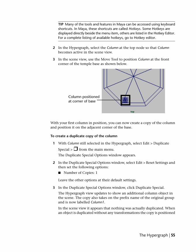
TIP Many of the tools and features in Maya can be accessed using keyboardshortcuts. In Maya, these shortcuts are called Hotkeys. Some Hotkeys aredisplayed directly beside the menu item, others are listed in the Hotkey Editor.For a complete listing of available hotkeys, go to Hotkey editor.
2 In the Hypergraph, select the Column at the top node so that Columnbecomes active in the scene view.
3 In the scene view, use the Move Tool to position Column at the frontcorner of the temple base as shown below.
With your first column in position, you can now create a copy of the columnand position it on the adjacent corner of the base.
To create a duplicate copy of the column
1 With Column still selected in the Hypergraph, select Edit > Duplicate
Special > from the main menu.
The Duplicate Special Options window appears.
2 In the Duplicate Special Options window, select Edit > Reset Settings andthen set the following options:
■ Number of Copies: 1
Leave the other options at their default settings.
3 In the Duplicate Special Options window, click Duplicate Special.
The Hypergraph view updates to show an additional column object inthe scene. The copy also takes on the prefix name of the original groupand is now labelled Column1.
In the scene view it appears that nothing was actually duplicated. Whenan object is duplicated without any transformations the copy is positioned
The Hypergraph | 55
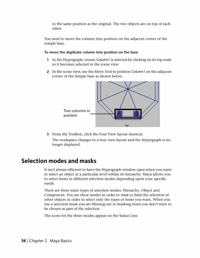
in the same position as the original. The two objects are on top of eachother.
You need to move the column into position on the adjacent corner of thetemple base.
To move the duplicate column into position on the base
1 In the Hypergraph, ensure Column1 is selected by clicking on its top nodeso it becomes selected in the scene view.
2 In the scene view, use the Move Tool to position Column1 on the adjacentcorner of the temple base as shown below.
3 From the Toolbox, click the Four View layout shortcut.
The workspace changes to a four view layout and the Hypergraph is nolonger displayed.
Selection modes and masksIt isn’t always efficient to have the Hypergraph window open when you wantto select an object at a particular level within its hierarchy. Maya allows youto select items in different selection modes depending upon your specificneeds.
There are three main types of selection modes: Hierarchy, Object andComponent. You use these modes in order to mask or limit the selection ofother objects in order to select only the types of items you want. When youuse a selection mask you are filtering out or masking items you don’t want tobe chosen as part of the selection.
The icons for the three modes appear on the Status Line.
56 | Chapter 2 Maya Basics

When you first start Maya, the default selection mode is set to Objects. Thisis useful for much of your selection work with Maya, with a few exceptions.When you want to select items that have been grouped, set the selection modeto Hierarchy.
TIP If you set the selection mask, it will remain that way until you change it again.If an item won’t select for you in Maya, you should check the selection mask settingto see if it is set correctly.
To use the Hierarchy and Combinations selection mask
1 On the Status Line, choose the Select by Hierarchy and Combinationsicon
The Selection Mask icons update to display the three selection choices.
2 On the Status Line, choose the Select by hierarchy icon.
Select by hierarchy ensures that when you select items they are selectedat their parent or root node.
3 In the scene view, shift-click Column and Column1 so they are selectedsimultaneously. (Do not be concerned that they highlight in differentcolors.)
Pivot pointsA pivot point is a specific position in 3D space that is used as a reference forthe transformations of objects. All objects (curves, surfaces, groups) have pivotpoints.
When you group objects in Maya, a new node called a parent node is createdfor the group of objects. The pivot point for the group’s parent node is placedat the origin (0, 0, 0). This is useful if you later want to duplicate and rotatethe objects radially (that is, in a circular fashion around the pivot).
Pivot points | 57

To group the two columns
1 Ensure Column and Column1 are selected.
2 From the main menu, select Edit > Group > .
3 In the Group Options window, select Edit > Reset Settings. Set thefollowing options:
■ Group Under: Parent
4 In the Group Options window, click Group.
Maya groups the objects together in a hierarchy and the pivot point ispositioned at the origin. (When the pivot point is relocated to the originthe Move Tool manipulator for the selected group appears at the origin.)
With the two columns grouped, you then duplicate the columns with arotation option, the groups will duplicate and rotate around the pivot pointat the origin (0, 0, 0).
To duplicate and rotate the group
1 With column group selected, select Edit > Duplicate Special > fromthe main menu.
2 In the Duplicate Special Options window, select Edit > Reset Settings andthen set the following options:
■ Rotate: 0 90 0
■ Number of Copies: 3
3 In the Duplicate Special Options window, click Duplicate Special.
The columns are duplicated and rotated by 90 degrees with each copy.
58 | Chapter 2 Maya Basics

Save your workYour temple is taking shape! Save your work before proceeding to the nextlesson.
To save your Maya scene
1 To save your Maya scene, select File > Save Scene As.
2 Type Lesson3Columns in the file browser area reserved for file names.
3 Click Save.
Beyond the lessonIn this lesson, you explored additional tools and skills within Maya as youcontinued with the construction of the classic temple. In this lesson youlearned how to:
■ Use your mouse to change the view of your scene using the dolly, track,and tumble camera tools in both the orthographic and perspective views.
■ Rotate objects using the transformation tools in the Toolbox and theChannel Box.
■ Group objects so they can be transformed as a unit.
■ Display objects in both wire frame and shaded modes.
■ Access the Hypergraph to view nodes and hierarchies. You are also learningthat many tasks in Maya can be completed or approached using multipletechniques.
■ Rename nodes within the Hypergraph.
■ Select objects in your scene using the Hypergraph.
■ Use the group pivot point to your advantage when duplicating objects.
Before proceeding with the next lesson you may want to review the materialpresented in this lesson so you are familiar with the concepts and skillsassociated with them. Some suggested tasks you can try on your own include:
■ Practice using the view camera tools (dolly, track, and tumble) so you cannavigate within the scene views efficiently.
Save your work | 59
■ Practice moving and rotating objects, and changing between the variousscene views (single perspective, four view, single side, single top, and soon).
■ View objects in the Hypergraph so you can understand their relationshipsand hierarchy.
Lesson 4: Components and attributes
IntroductionWorking with components is an important part of the workflow when workingin Maya. Components describe objects at a more detailed level. As you editthe components of your classic temple, you will learn more about what ispossible in Maya.
In this lesson you learn how to:
■ Template objects in the scene.
■ Understand the difference between objects and components.
■ Edit objects at their component level.
■ Assign surface material attributes
■ Access the Attribute editor
Template displayWhen your scene becomes complex, templating the display of some of theobjects in your scene allows you to more easily select only the objects youwant. When you template the display of an object, its wireframe changes toa gray color. The object(s) can still be seen, but not easily selected. This helpsto prevent you from selecting or modifying it accidentally. You can changethe display of objects to a template and use them as a modeling reference (theway a grid is used).
You need to change the display of the base and columns to template modeso that you can more easily work on the temple roof.
60 | Chapter 2 Maya Basics

To template the base and columns
1 In the side view, with the Selection Mask set to Hierarchy, select all theobjects in your scene.
2 From the main menu, select Display > Object Display > Template.
The selected objects become templated.
For your classic temple, you need to create the entablature using a torusprimitive. An entablature is a structure that lies horizontally upon the columnsof a temple and supports the roof.
To create and position a torus primitive for the entablature
1 From the main menu, select Create > NURBS Primitives > Torus > .
2 In the NURBS Torus Options window, select Edit > Reset Settings andthen set the following options:
■ Radius: 8.5
■ Minor Radius: 0.5
■ Number of Sections: 24
3 In the NURBS Torus option window, click Create.
NOTE If the NURBS Primitives Options window does not appear, ensure thata check mark does not appear beside the Interactive Creation menu item
before selecting Create > NURBS Primitives > Torus > by first selectingCreate > NURBS Primitives > Interactive Creation.
4 In the Channel Box, rename the torus primitive Entablature.
5 Move the entablature vertically in the scene so it rests on top of thecolumns (Translate Y = 9.7).
Template display | 61

ComponentsAll objects in Maya have a transform and a shape node. Geometric shapes,like the primitives in this tutorial, have smaller parts called components. A fewexamples of components in Maya are control vertices, faces, and hulls.Components allow you to work with objects at a finer level and allow you toedit them in creative ways.
In order to change the shape of the entablature beyond the basic scaletransformations, you need to modify its component information.
To select components of the entablature
1 In the side view, dolly in for a closer view of Entablature.
2 Set the Selection Mode to Component mode.
3 Right-click the wireframe of Entablature and select Control Vertex fromthe pop-up menu.
62 | Chapter 2 Maya Basics
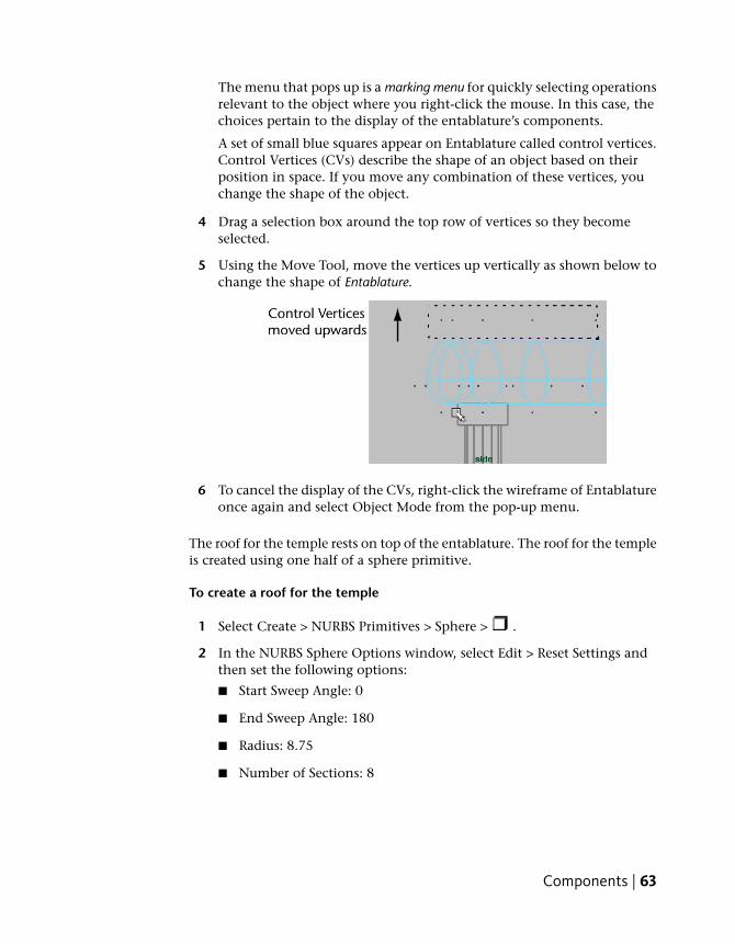
The menu that pops up is a marking menu for quickly selecting operationsrelevant to the object where you right-click the mouse. In this case, thechoices pertain to the display of the entablature’s components.
A set of small blue squares appear on Entablature called control vertices.Control Vertices (CVs) describe the shape of an object based on theirposition in space. If you move any combination of these vertices, youchange the shape of the object.
4 Drag a selection box around the top row of vertices so they becomeselected.
5 Using the Move Tool, move the vertices up vertically as shown below tochange the shape of Entablature.
6 To cancel the display of the CVs, right-click the wireframe of Entablatureonce again and select Object Mode from the pop-up menu.
The roof for the temple rests on top of the entablature. The roof for the templeis created using one half of a sphere primitive.
To create a roof for the temple
1 Select Create > NURBS Primitives > Sphere > .
2 In the NURBS Sphere Options window, select Edit > Reset Settings andthen set the following options:
■ Start Sweep Angle: 0
■ End Sweep Angle: 180
■ Radius: 8.75
■ Number of Sections: 8
Components | 63
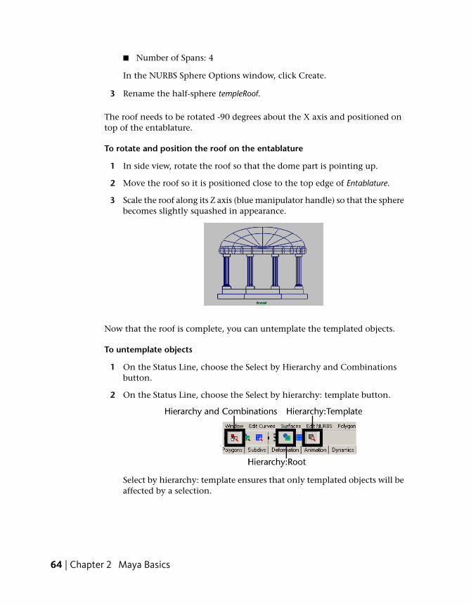
■ Number of Spans: 4
In the NURBS Sphere Options window, click Create.
3 Rename the half-sphere templeRoof.
The roof needs to be rotated -90 degrees about the X axis and positioned ontop of the entablature.
To rotate and position the roof on the entablature
1 In side view, rotate the roof so that the dome part is pointing up.
2 Move the roof so it is positioned close to the top edge of Entablature.
3 Scale the roof along its Z axis (blue manipulator handle) so that the spherebecomes slightly squashed in appearance.
Now that the roof is complete, you can untemplate the templated objects.
To untemplate objects
1 On the Status Line, choose the Select by Hierarchy and Combinationsbutton.
2 On the Status Line, choose the Select by hierarchy: template button.
Select by hierarchy: template ensures that only templated objects will beaffected by a selection.
64 | Chapter 2 Maya Basics

3 In the scene view, drag a selection box around all the objects in the sceneso that the templated objects are selected simultaneously.
4 From the main menu, select Display > Object Display > Untemplate.
5 On the Status Line, choose the Select by hierarchy: root button.
The Attribute EditorThe Attribute Editor provides information about the various nodes andattributes for the objects and materials in your scene. Like the Channel Box,you can view and edit the basic transform information and many other keyableattributes. However, the Attribute Editor provides a more detailed display ofall attributes for a selected object.
To view object attributes using the Attribute Editor
1 In the scene view, select templeRoof so it becomes the selected object.
2 To view the Attribute Editor, click the Show/Hide icon on the Status Line.
The Attribute Editor displays the attributes for templeRoof. The variousattributes for the templeRoof object appear under various tabs. Each tabrepresents a node.
The Attribute Editor | 65
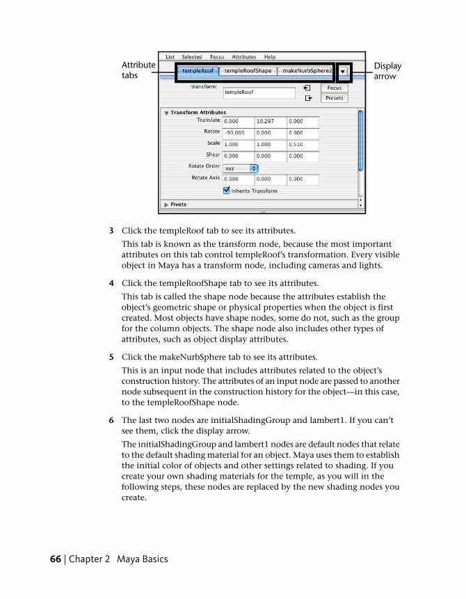
3 Click the templeRoof tab to see its attributes.
This tab is known as the transform node, because the most importantattributes on this tab control templeRoof’s transformation. Every visibleobject in Maya has a transform node, including cameras and lights.
4 Click the templeRoofShape tab to see its attributes.
This tab is called the shape node because the attributes establish theobject’s geometric shape or physical properties when the object is firstcreated. Most objects have shape nodes, some do not, such as the groupfor the column objects. The shape node also includes other types ofattributes, such as object display attributes.
5 Click the makeNurbSphere tab to see its attributes.
This is an input node that includes attributes related to the object’sconstruction history. The attributes of an input node are passed to anothernode subsequent in the construction history for the object—in this case,to the templeRoofShape node.
6 The last two nodes are initialShadingGroup and lambert1. If you can’tsee them, click the display arrow.
The initialShadingGroup and lambert1 nodes are default nodes that relateto the default shading material for an object. Maya uses them to establishthe initial color of objects and other settings related to shading. If youcreate your own shading materials for the temple, as you will in thefollowing steps, these nodes are replaced by the new shading nodes youcreate.
66 | Chapter 2 Maya Basics

Surface materialsThe color, shininess, and reflectivity attributes of an object are controlled byits surface material (sometimes referred to as a shader, or shading material).Material attributes relate to how the object simulates a natural reaction tolight in Maya’s 3D computer world.
Maya assigns a default shading material to all objects when they are firstcreated. In this section, you learn how to assign a new material to your objects.
To assign a new material to the temple objects
1 Right-click the wireframe of Entablature and select Object Mode fromthe pop-up menu.
This changes the selection mask back to objects so you can select objectsin the scene. It is a shortcut to access this feature.
2 Drag a selection box around all the objects in your scene to select them.
TIP If objects won’t select in the Maya scene, check that your selection maskis set correctly on the Status Line.
3 From the Status Line, select the Rendering menu set using the menuselector.
The main menu changes to display the menu set for Rendering.
4 From the main menu, select Lighting/Shading > Assign New Material >Blinn.
A Blinn shading material is assigned to all the objects in the scene andthe Attribute Editor updates. Blinn shading materials (named after the
Surface materials | 67
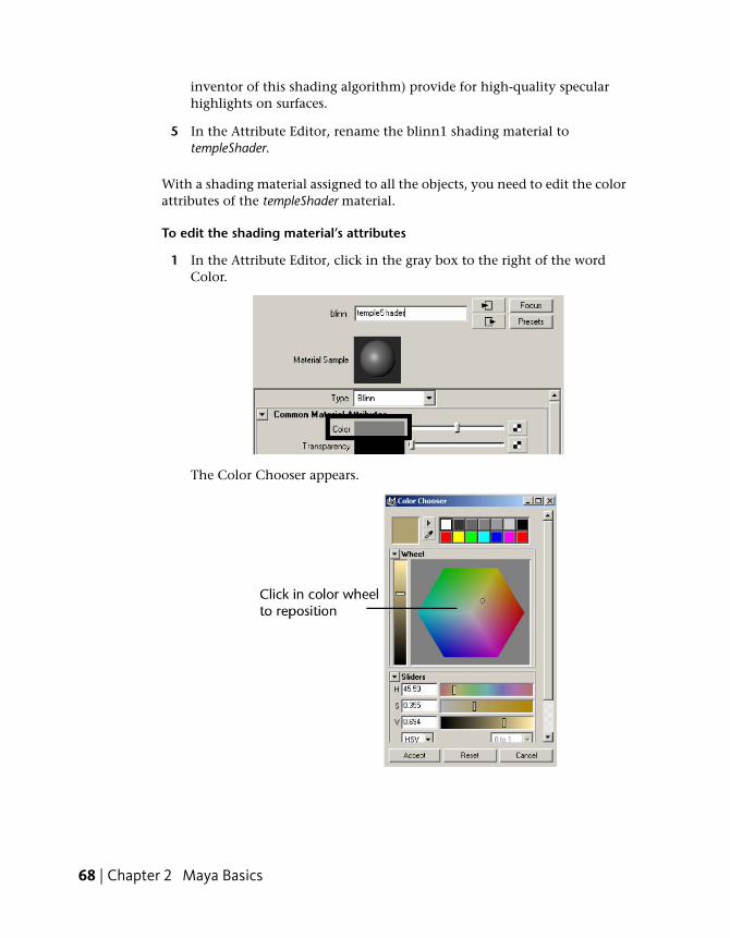
inventor of this shading algorithm) provide for high-quality specularhighlights on surfaces.
5 In the Attribute Editor, rename the blinn1 shading material totempleShader.
With a shading material assigned to all the objects, you need to edit the colorattributes of the templeShader material.
To edit the shading material’s attributes
1 In the Attribute Editor, click in the gray box to the right of the wordColor.
The Color Chooser appears.
68 | Chapter 2 Maya Basics
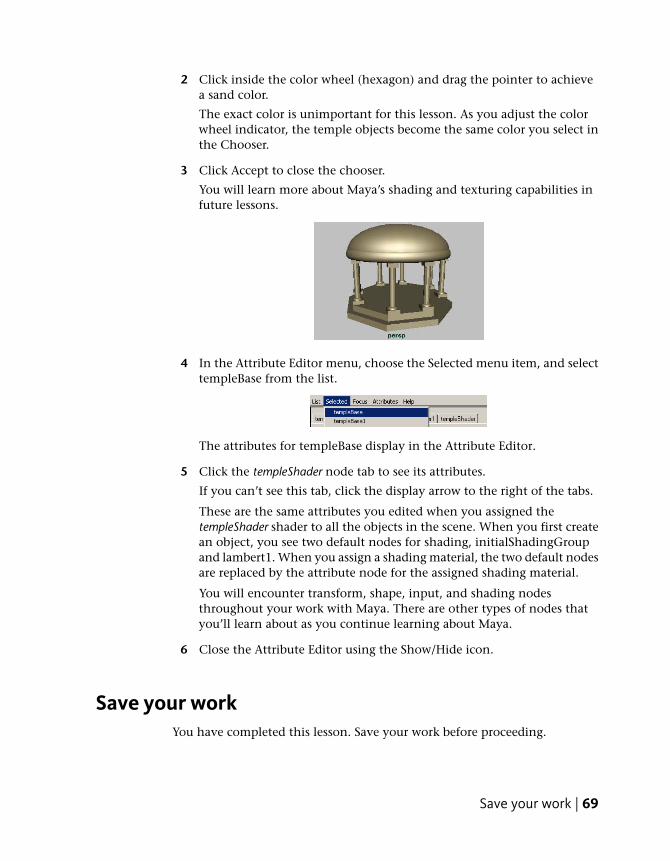
2 Click inside the color wheel (hexagon) and drag the pointer to achievea sand color.
The exact color is unimportant for this lesson. As you adjust the colorwheel indicator, the temple objects become the same color you select inthe Chooser.
3 Click Accept to close the chooser.
You will learn more about Maya’s shading and texturing capabilities infuture lessons.
4 In the Attribute Editor menu, choose the Selected menu item, and selecttempleBase from the list.
The attributes for templeBase display in the Attribute Editor.
5 Click the templeShader node tab to see its attributes.
If you can’t see this tab, click the display arrow to the right of the tabs.
These are the same attributes you edited when you assigned thetempleShader shader to all the objects in the scene. When you first createan object, you see two default nodes for shading, initialShadingGroupand lambert1. When you assign a shading material, the two default nodesare replaced by the attribute node for the assigned shading material.
You will encounter transform, shape, input, and shading nodesthroughout your work with Maya. There are other types of nodes thatyou’ll learn about as you continue learning about Maya.
6 Close the Attribute Editor using the Show/Hide icon.
Save your workYou have completed this lesson. Save your work before proceeding.
Save your work | 69

To save your Maya scene
1 Select File > Save Scene As.
2 Type Lesson4Final in the file browser area reserved for file names, andthen click Save.
Beyond the lessonIn this lesson, you completed the construction of the classic temple and learnedhow to:
■ Display objects in template mode.
■ Select objects at their component level using selection masks and the rightmouse button.
■ Assign and edit shading materials for your objects in the scene.
■ Access the Attribute editor and view the various node types for objects.
As you proceed through Getting Started with Maya, we assume you are familiarwith the fundamental concepts and skills covered in this first chapter.
Before proceeding to the next chapter you may want to review the materialpresented in this lesson so you are familiar with the concepts and skillsassociated with them. Some suggested tasks you may want to do on your own:
■ Practice construction of additional forms using primitive shapes by creating.additional details for your temple scene (stairs, roof details, etc.).
■ Learn more about the tools and options that have been presented in thislesson, by referring to the Maya Help. To view the Maya Help, select Help> Maya Help.
70 | Chapter 2 Maya Basics

Polygonal Modeling
Introduction
In Maya, modeling refers to the process of creating virtual 3D surfaces for thecharacters and objects in the Maya scene. Surfaces are vital for creating aconvincing 3D image.
Modeling is a process requiring keen visual skills and mastery of the modelingtools. The more accurate you are when modeling your forms in terms of size,shape, detail, and proportion, the more convincing your final scene will be.
There are three modeling surface types in Maya:
■ Polygons
■ NURBS
■ Subdivision surfaces.
Each surface type has particular characteristics and benefits.
3
71

Polygon surfaces are a network of three-or-more sided flat surfaces called facesthat get connected together to create a poly mesh. Polygon meshes arecomprised of vertices, faces, and edges.
The wireframe lines on the mesh represent the edges of each face. The regionsbounded by the edges are faces. Where the edges intersect each other is thelocation of a point called a vertex.
When a polygon mesh is rendered, its edges can be set to appear hard orsmooth. As a result, polygons can easily represent both flat as well as curved3D forms. You’ll work with these component types continuously whenmodeling with polygons.
Polygonal surfaces have a wide range of applications and are the preferredsurface type for many 3D applications including interactive games and webdevelopment applications.
Polygonal surfaces can be described with the smallest amount of data of allthe 3D surface types, and therefore, can be rendered quickly, deliveringincreased speed and interactive performance to the end user in games andother applications.
Preparing for the lessonTo ensure the lesson works as described, do these steps before beginning:
1 Select File > New Scene.
2 Make sure Construction History (below the menu bar) is on: . (If itis turned off, the icon has a large X across it).
3 Select the Polygons menu set.
Unless otherwise noted, the directions in this chapter for making menuselections assume you’ve already selected the Polygons menu set.
4 Make sure Display > UI Elements > Help Line is turned on.
You will use the Help Line while modeling.
5 If you have not already done so, copy the GettingStarted folder fromits installation location to your projects directory. Then, set theGettingStarted directory as your Maya project. For more information,see Copying and setting the Maya project on page 25.
72 | Chapter 3 Polygonal Modeling

6 As you work through this lesson, remember to save your work frequentlyand increment the name of the file every so often (filename1, filename2,and so on).
In this way you’ll have earlier versions of your work to return to shouldthe need arise.
7 Make sure that Soft Selection is turned off by opening the Tool SettingsEditor with the Select Tool active and unchecking the box marked SoftSelect.
Lesson 1: Modeling a polygonal mesh
Introduction
In this lesson, you model a helmet for an interactive game character, usingpolygonal surface modeling techniques.
In this lesson you’ll be introduced to some of the polygon modeling toolsMaya provides by learning how to:
■ Use 2D image planes as a reference for constructing 3D models
■ Use 3D primitives as the basis for creating more complex models
■ Work with the components of a polygon mesh (faces, edges, and vertices)
■ Smooth a polygon mesh
■ Select the faces, edges, and vertices of polygonal meshes
Lesson 1: Modeling a polygonal mesh | 73

■ Create polygon faces by placing vertices
■ Scale and extrude faces on a polygon mesh
■ Move and rotate extruded polygonal meshes
■ Split vertices and subdivide polygonal faces
■ Combine separate meshes into one mesh
■ Bridge between meshes
■ Add faces to an existing mesh
■ Use Snap to Grid
■ Preview a smoothed high resolution version of a polygon mesh
■ Harden and soften polygon edges
Setting modeling preferencesBefore you create your polygon model change some of the default settings tobetter work through this lesson.
1 Select Window > Settings/Preferences > Preferences.
The Maya user preferences window appears.
In the Categories section of the Preferences window select Polygons.
2 In the Polygon Display settings, set the following:
■ Border Edges: On
■ Edge Width: 4
This displays border edges prominently on polygon meshes. Displayingborder edges distinctively lets you differentiate them from other edgeson your models and troubleshoot issues.
3 In the Categories section of the Preferences window, choose Selection.
4 In the Polygon Selection settings, set the following:
■ Select faces with: Whole face
The Whole face setting lets you select polygon faces by clicking anywhereon the face (the Center setting requires you to click on the face’s center
74 | Chapter 3 Polygonal Modeling
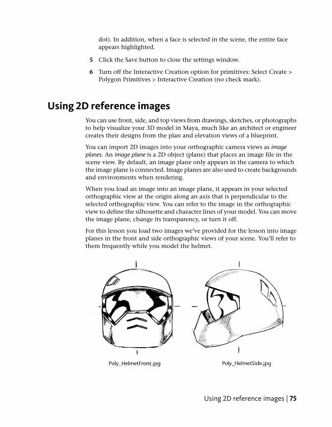
dot). In addition, when a face is selected in the scene, the entire faceappears highlighted.
5 Click the Save button to close the settings window.
6 Turn off the Interactive Creation option for primitives: Select Create >Polygon Primitives > Interactive Creation (no check mark).
Using 2D reference imagesYou can use front, side, and top views from drawings, sketches, or photographsto help visualize your 3D model in Maya, much like an architect or engineercreates their designs from the plan and elevation views of a blueprint.
You can import 2D images into your orthographic camera views as imageplanes. An image plane is a 2D object (plane) that places an image file in thescene view. By default, an image plane only appears in the camera to whichthe image plane is connected. Image planes are also used to create backgroundsand environments when rendering.
When you load an image into an image plane, it appears in your selectedorthographic view at the origin along an axis that is perpendicular to theselected orthographic view. You can refer to the image in the orthographicview to define the silhouette and character lines of your model. You can movethe image plane, change its transparency, or turn it off.
For this lesson you load two images we’ve provided for the lesson into imageplanes in the front and side orthographic views of your scene. You’ll refer tothem frequently while you model the helmet.
Using 2D reference images | 75
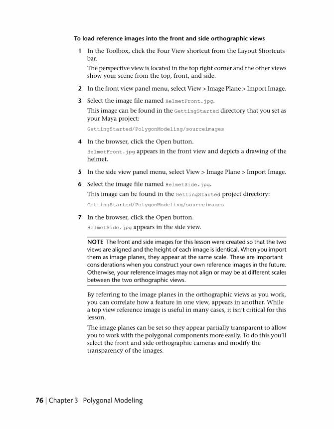
To load reference images into the front and side orthographic views
1 In the Toolbox, click the Four View shortcut from the Layout Shortcutsbar.
The perspective view is located in the top right corner and the other viewsshow your scene from the top, front, and side.
2 In the front view panel menu, select View > Image Plane > Import Image.
3 Select the image file named HelmetFront.jpg.
This image can be found in the GettingStarted directory that you set asyour Maya project:
GettingStarted/PolygonModeling/sourceimages
4 In the browser, click the Open button.
HelmetFront.jpg appears in the front view and depicts a drawing of thehelmet.
5 In the side view panel menu, select View > Image Plane > Import Image.
6 Select the image file named HelmetSide.jpg.
This image can be found in the GettingStarted project directory:
GettingStarted/PolygonModeling/sourceimages
7 In the browser, click the Open button.
HelmetSide.jpg appears in the side view.
NOTE The front and side images for this lesson were created so that the twoviews are aligned and the height of each image is identical. When you importthem as image planes, they appear at the same scale. These are importantconsiderations when you construct your own reference images in the future.Otherwise, your reference images may not align or may be at different scalesbetween the two orthographic views.
By referring to the image planes in the orthographic views as you work,you can correlate how a feature in one view, appears in another. Whilea top view reference image is useful in many cases, it isn’t critical for thislesson.
The image planes can be set so they appear partially transparent to allowyou to work with the polygonal components more easily. To do this you’llselect the front and side orthographic cameras and modify thetransparency of the images.
76 | Chapter 3 Polygonal Modeling
To modify the transparency of the reference images
1 In the front view panel menu, select View > Select Camera.
The camera for the front orthographic view is selected.
2 Display the Channel Box by clicking the Show/Hide Channel Box iconon the Status Line.
The Channel Box displays the keyable attributes for the Frontorthographic camera.
3 In the Inputs section, click the ImagePlane1 name to display the attributesfor the image plane.
4 Set the Alpha Gain attribute to a value of 0.25.
The image appears partially transparent.
5 In the side view panel menu, select the camera and change the AlphaGain setting for the side view image plane exactly as you changed thefront view image plane.
TIP You can change the Alpha Gain at any time if you want the image planesto appear more or less transparent.
6 In the perspective view’s panel menu, select Show > Cameras totemporarily turn off the display of the image planes in the perspectiveview.
Using 2D reference images | 77

Creating a polygon primitiveYou’ll create the top portion of the helmet mesh from a cube primitive usingthe image planes as a reference. Primitive objects are one method for starting3D meshes because they can be modified to create other forms.
To create a cube primitive for the helmet mesh
1 Ensure you are working in the perspective view.
2 Select Create > Polygon Primitives > Cube > .
3 In the options window, select Edit > Reset Settings, and then set thefollowing:
■ Width: 14
■ Height: 14
■ Depth: 14
■ Width divisions: 1
■ Height divisions: 2
■ Depth divisions: 1
4 Click the Create button.
A cube primitive is created at the origin with the dimensions you specifiedand one subdivision around the middle. This cube primitive is comprisedof four-sided polygon faces called quads. Quad polygons are usedfrequently with 3D character models as they are easily smoothed anddeform well when bound into a skeleton.
You can smooth the cube so it appears more rounded on the corners andsubdivide it into smaller faces using the Smooth feature.
78 | Chapter 3 Polygonal Modeling

To smooth and subdivide the cube primitive
1 With the cube still selected in the scene view, select Mesh > Smooth >
, and set the following options in the window that appears:
■ Add divisions: Exponentially
■ Division levels: 2
2 Click the Smooth button
The cube primitive is smoothed and is rounded at its corners. The cubehas also been subdivided into smaller faces.
The polygon faces are still four-sided even though their shape and positionhave been modified by the smooth operation.
NOTE If the top, domed portion of the smoothed cube doesn’t roughlymatch the helmet sketches as indicated in the image below, scale the cubewith the Scale Tool to make it match.
Creating a polygon primitive | 79

To rename the polygon mesh
➤ With the cube still selected, rename the cube primitive using the ChannelBox from pCube1 to helmetmesh.
Modeling in shaded modeModeling a polygon mesh in shaded mode gives you a better sense of the 3Dvolume that the model occupies as well as how any surface details appear.
You can control the shading of an object separately in each view. For example,you can display the object as shaded in the perspective view only, and set theorthographic views to display objects in wireframe mode. You can also set thedisplay settings to show both a shaded and wireframe display simultaneously.
To display the helmet mesh in Wireframe on Shaded mode
1 In the perspective view, right-click on the helmet mesh and select ObjectMode from the marking menu that appears.
This changes the selection mode to Objects.
2 Select the helmet mesh.
3 In the perspective view, select Shading > Smooth Shade All from the panelmenu.
The helmet mesh displays in smooth shaded mode.
4 From the panel menu, select Shading > Wireframe on Shaded.
80 | Chapter 3 Polygonal Modeling
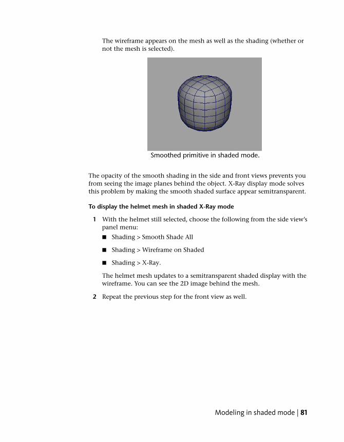
The wireframe appears on the mesh as well as the shading (whether ornot the mesh is selected).
The opacity of the smooth shading in the side and front views prevents youfrom seeing the image planes behind the object. X-Ray display mode solvesthis problem by making the smooth shaded surface appear semitransparent.
To display the helmet mesh in shaded X-Ray mode
1 With the helmet still selected, choose the following from the side view’spanel menu:
■ Shading > Smooth Shade All
■ Shading > Wireframe on Shaded
■ Shading > X-Ray.
The helmet mesh updates to a semitransparent shaded display with thewireframe. You can see the 2D image behind the mesh.
2 Repeat the previous step for the front view as well.
Modeling in shaded mode | 81
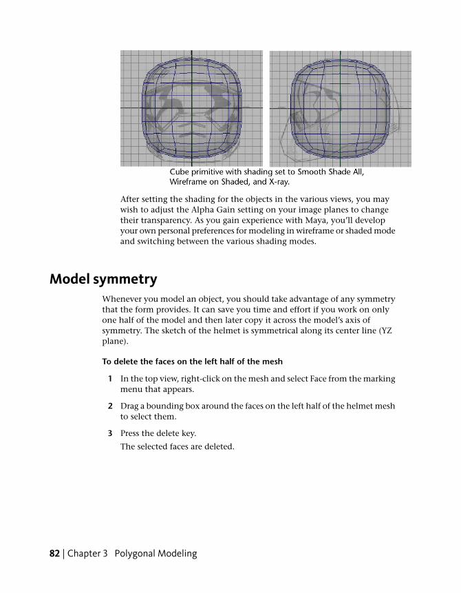
After setting the shading for the objects in the various views, you maywish to adjust the Alpha Gain setting on your image planes to changetheir transparency. As you gain experience with Maya, you’ll developyour own personal preferences for modeling in wireframe or shaded modeand switching between the various shading modes.
Model symmetryWhenever you model an object, you should take advantage of any symmetrythat the form provides. It can save you time and effort if you work on onlyone half of the model and then later copy it across the model’s axis ofsymmetry. The sketch of the helmet is symmetrical along its center line (YZplane).
To delete the faces on the left half of the mesh
1 In the top view, right-click on the mesh and select Face from the markingmenu that appears.
2 Drag a bounding box around the faces on the left half of the helmet meshto select them.
3 Press the delete key.
The selected faces are deleted.
82 | Chapter 3 Polygonal Modeling
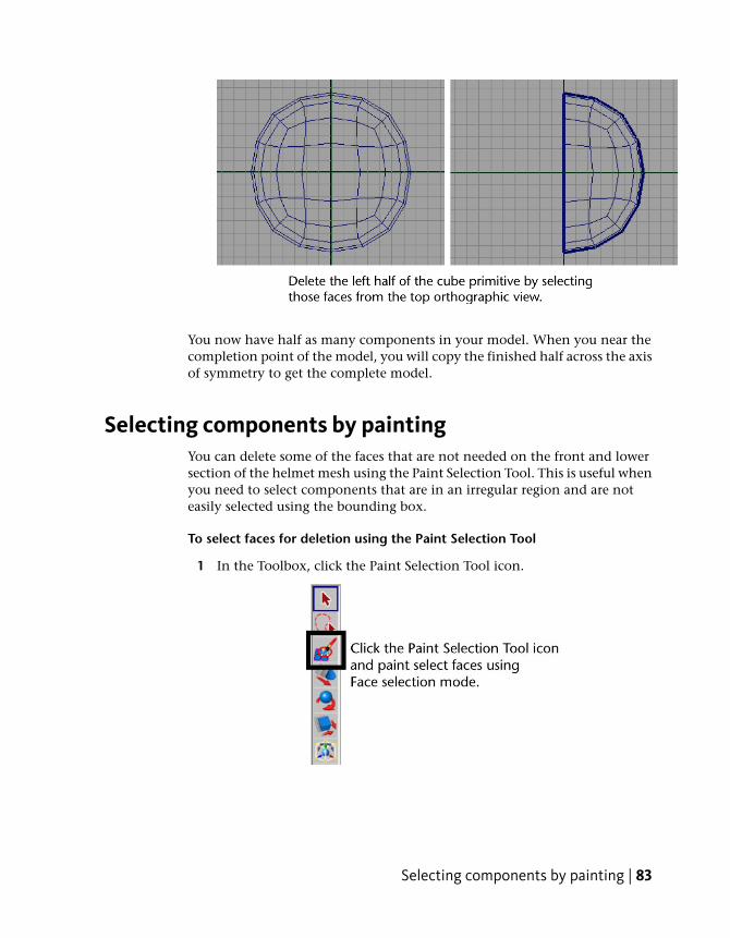
You now have half as many components in your model. When you near thecompletion point of the model, you will copy the finished half across the axisof symmetry to get the complete model.
Selecting components by paintingYou can delete some of the faces that are not needed on the front and lowersection of the helmet mesh using the Paint Selection Tool. This is useful whenyou need to select components that are in an irregular region and are noteasily selected using the bounding box.
To select faces for deletion using the Paint Selection Tool
1 In the Toolbox, click the Paint Selection Tool icon.
Selecting components by painting | 83

2 In the side view, right-click the helmet mesh and select Face from themarking menu that appears.
3 In the side view, paint select the faces that appear along the front andlower areas of the mesh (see image) by dragging the mouse over the faces.
NOTE The Paint Selection Tool only selects components on the mesh thatface towards the camera.
4 Press the delete key to delete the selected faces.
5 Tumble the perspective view to review your work so far.
The edges that reside along the outside perimeter of a polygon mesh,called border edges, are displayed with a thicker line than the interioredges on the mesh. You set this display setting early in the lesson so youcould differentiate this edge type from other edges.
Selecting edge loopsIn the top view, the rows of edges immediately above and below the X axis,and the row to the right of the Z axis are not straight. You’ll want to align theedges in these rows (referred to as edge loops) by snapping them to the gridusing the Move Tool. An edge loop is a path of polygon edges that are connectedin sequence by their shared vertices. Edge loop selections are very useful whenyou model using polygons.
84 | Chapter 3 Polygonal Modeling
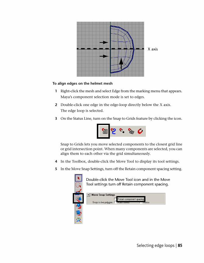
To align edges on the helmet mesh
1 Right-click the mesh and select Edge from the marking menu that appears.
Maya’s component selection mode is set to edges.
2 Double-click one edge in the edge-loop directly below the X axis.
The edge loop is selected.
3 On the Status Line, turn on the Snap to Grids feature by clicking the icon.
Snap to Grids lets you move selected components to the closest grid lineor grid intersection point. When many components are selected, you canalign them to each other via the grid simultaneously.
4 In the Toolbox, double-click the Move Tool to display its tool settings.
5 In the Move Snap Settings, turn off the Retain component spacing setting.
Selecting edge loops | 85

6 In the top view, click-drag the blue arrow on the Move Tool manipulatordownwards a small distance.
The edge loop immediately snaps to a lower grid line. It is not positionedat the location you want, but all of the edges in the loop you selected arenow aligned to each other.
7 On the Status Line, turn off the Snap to Grids feature by clicking its icon.
8 With the Move Tool still active in the top view, drag the manipulatorarrow upwards a short distance so the edge loop is positioned roughly atits original location (which should be at the second grid line below theX axis).
9 Using the steps described above, align the other edge loop that appearsabove the X axis and then align the edge loop directly to the right of theZ axis. (Remember to turn on and off Snap to Grids as required.)
When you have finished, the edge loops nearest the X and Z axes arealigned. (see image below)
Editing components in the orthographic viewsComponent selection and transformation is one fundamental method forediting the shape of a polygon mesh. As you model, you’ll find yourselffrequently examining and then refining the position of the polygoncomponents (vertices, edges, and faces) while working in the various sceneviews so they match the reference images on the image planes.
86 | Chapter 3 Polygonal Modeling

To manually reposition the vertices on the rear of the helmet
1 Right-click the helmet and select Vertex from the marking menu thatappears.
2 In the side view, select the pair of vertices at the rear lower edge (seeimage) by dragging a bounding box around them.
3 In the Toolbox, click the Move Tool.
4 In the side view, click-drag the blue arrow on the Move Tool manipulatortowards the right until the vertices are repositioned so that your helmetmatches the reference sketch on the image plane.
By moving the vertex as well as the vertex adjacent to it along the axisof symmetry, you ensure that the symmetrical shape of the helmet ismaintained. If you move one vertex independently of the other it mayresult in an unwanted bump or valley in the mesh. These types ofanomalies will become more apparent when you copy the completedhalf of the mesh across the axis of symmetry.
5 Repeat steps 2 through 4 for the other pairs of vertices on the rear of thehelmet. Ensure that the edge loops appear smooth in relation to eachother.
When you have finished, the back region of the helmet should closelymatch the reference image on your image plane.
Editing components in the orthographic views | 87

6 In the side view, select other pairs of vertices along the top and front ofthe helmet and move them in a similar fashion so they match thereference image. Do not reposition the vertices for the top of the faceshield yet.
TIP You can click in the center of the Move Tool manipulator to drag a vertexselection freely.
Next, you’ll reposition the border edges that lie along the bottom edge of themesh. You can select these edge types using the Select Border Edge Tool.
To reposition the lower border edges on the helmet
1 In the side view, select the lowest horizontal edge loop on the helmet bychoosing Select > Select Border Edge Toolfrom the main menu, and then
88 | Chapter 3 Polygonal Modeling

clicking the first and then the last edge on the loop as indicated in theimage below.
2 Using the Move Tool, drag the selected edge loop downwards until theleft hand vertex roughly matches the lower edge indicated in the referencesketch.
3 In the side view, select and reposition the remaining vertices individuallyon the edge loop using the Move Tool so they match the reference sketch.
NOTE Up to this point in the lesson, you’ve been instructed to repositionthe vertices on the helmet mesh only within the side view (Y, Z plane). Onceyou achieve the shape you want in the side view you will then concentrateon how the model appears when viewed from the front and perspectiveviews.
Editing components in the orthographic views | 89

To edit the border edges on the upper edge of the face shield
1 From the Select menu, choose Select Border Edge Tool.
2 In the side view, click the first border edge that will be used as the upperedge of the face shield, then click the last border edge (see image).
The border edges in between are selected.
3 In the Toolbox, select the Rotate Tool by clicking its icon.
4 In the side view, click-drag the rotate manipulator in a clockwise directionuntil the border edges are rotated at roughly the same angle as thecorresponding edge in the reference sketch.
5 With the border edges still selected, click the Move Tool again and dragthe green manipulator upwards to match the location of the border edgesin the reference sketch.
90 | Chapter 3 Polygonal Modeling

6 Reposition the pairs of vertices on the upper front of the helmet to matchthe reference sketch.
At this point in the lesson, the outline of your helmet should roughly matchthe helmet in the side view reference image. If it doesn’t, review the earliersteps in this lesson and make any adjustments to your polygonal mesh asrequired.
If you view your helmet in the front orthographic view, you’ll notice that thehelmet shows a wider profile from this view than the reference sketch. In thenext steps you’ll correct this using the front and top orthographic views ofthe helmet for reference.
To reposition vertices on the side of the helmet to match the sketch
1 Display the front view.
Editing components in the orthographic views | 91

2 In the front view, select the vertices that extend beyond the outline ofthe helmet as shown in the reference sketch (see image).
3 In the front view, move these vertices to the left until they match thewidest area of the helmet in the reference sketch (see image).
When you view your helmet from the top orthographic view the regionbetween the side and rear of the helmet appears a bit flat in relation to theother areas. To correct this you can move the other vertices in this regionoutwards in a similar fashion so the curvature in this area appears fuller andmore rounded. However, viewing only from the orthographic views can belimiting, and you should also use the perspective view to examine the mesh.
92 | Chapter 3 Polygonal Modeling
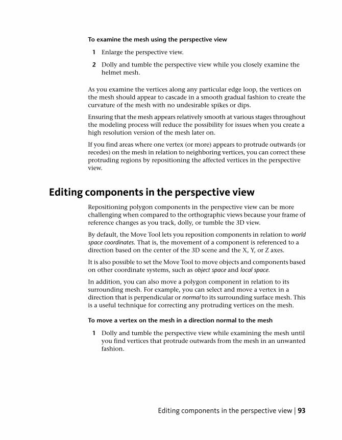
To examine the mesh using the perspective view
1 Enlarge the perspective view.
2 Dolly and tumble the perspective view while you closely examine thehelmet mesh.
As you examine the vertices along any particular edge loop, the vertices onthe mesh should appear to cascade in a smooth gradual fashion to create thecurvature of the mesh with no undesirable spikes or dips.
Ensuring that the mesh appears relatively smooth at various stages throughoutthe modeling process will reduce the possibility for issues when you create ahigh resolution version of the mesh later on.
If you find areas where one vertex (or more) appears to protrude outwards (orrecedes) on the mesh in relation to neighboring vertices, you can correct theseprotruding regions by repositioning the affected vertices in the perspectiveview.
Editing components in the perspective viewRepositioning polygon components in the perspective view can be morechallenging when compared to the orthographic views because your frame ofreference changes as you track, dolly, or tumble the 3D view.
By default, the Move Tool lets you reposition components in relation to worldspace coordinates. That is, the movement of a component is referenced to adirection based on the center of the 3D scene and the X, Y, or Z axes.
It is also possible to set the Move Tool to move objects and components basedon other coordinate systems, such as object space and local space.
In addition, you can also move a polygon component in relation to itssurrounding mesh. For example, you can select and move a vertex in adirection that is perpendicular or normal to its surrounding surface mesh. Thisis a useful technique for correcting any protruding vertices on the mesh.
To move a vertex on the mesh in a direction normal to the mesh
1 Dolly and tumble the perspective view while examining the mesh untilyou find vertices that protrude outwards from the mesh in an unwantedfashion.
Editing components in the perspective view | 93

2 In the Toolbox, double-click the Move Tool to display the Move Settingseditor.
3 In the Move Settings editor, in the Move section, turn on the Normaloption.
4 In the perspective view, click the vertex you wish to reposition.
The vertex highlights and the Move manipulator appears to indicate thethree directions of movement that are possible in this mode.
The U and V handles slide the vertex in relation to its associated edges,while the N handle moves the vertex either away or towards the meshdepending on the direction you move your mouse.
94 | Chapter 3 Polygonal Modeling
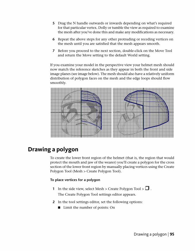
5 Drag the N handle outwards or inwards depending on what’s requiredfor that particular vertex. Dolly or tumble the view as required to examinethe mesh after you’ve done this and make any modifications as necessary.
6 Repeat the above steps for any other protruding or receding vertices onthe mesh until you are satisfied that the mesh appears smooth.
7 Before you proceed to the next section, double-click on the Move Tooland return the Move setting to the default World setting.
If you examine your model in the perspective view your helmet mesh shouldnow match the reference sketches as they appear in both the front and sideimage planes (see image below). The mesh should also have a relatively uniformdistribution of polygon faces on the mesh and the edge loops should flowsmoothly.
Drawing a polygonTo create the lower front region of the helmet (that is, the region that wouldprotect the mouth and jaw of the wearer) you’ll create a polygon for the crosssection of the lower front region by manually placing vertices using the CreatePolygon Tool (Mesh > Create Polygon Tool).
To place vertices for a polygon
1 In the side view, select Mesh > Create Polygon Tool > .
The Create Polygon Tool settings editor appears.
2 In the tool settings editor, set the following options:
■ Limit the number of points: On
Drawing a polygon | 95

■ Limit points to: 6
These settings specify that a closed polygon face will be created once youhave placed six vertices in the scene.
3 In the side view, place six points for the profile as it appears in crosssection of the lower front region of the helmet (see image below). Ensurethat you place the vertices in a counter-clockwise direction for this step.
The new polygon face is created along the YZ plane (the axis of symmetryfor the model).
4 Press the q key to quit the Create Polygon Tool when the polygon faceis complete.
The new polygon component remains selected in Object Mode.
NOTE If the polygon face doesn’t appear shaded in the side view but doesappear shaded in the perspective view, it means that the polygon face andthe image plane lie on exactly the same plane. You can correct this by movingthe image plane backwards in the side view so it doesn’t lie directly on theYZ plane, but this step is not critical to the success of the steps that follow.
You’ll extrude this polygon face to create the remainder of the lower frontregion of the helmet. Before you can extrude the new face it needs to beselected in Face mode. You can do this quickly by converting the existingselection to Faces.
To convert the object selection to face selection
➤ With the face still active in Object Mode, choose Select > ConvertSelection > To Faces.
96 | Chapter 3 Polygonal Modeling

The selection is converted to a face selection.
TIP You can also press Ctrl + F11 or Ctrl + right-click on the selected objectand choose To Faces > To Faces from the marking menu that appears.
Extruding polygon componentsYou can create new polygon components from existing ones using the Extrudefeature (Edit Mesh > Extrude). When you extrude a polygon component (forexample, a face, edge, or vertex), you create additional polygon componentsfrom the ones you selected. Using the Extrude feature you will:
■ Create the lower front region of the helmet by extruding the polygon faceyou created in the last section of the lesson.
■ Extrude edges around the face shield and along the lower bottom edge.
To extrude the polygon face for the lower front region
1 Enlarge the scene view to a single perspective view.
2 With the polygon face still selected, choose Edit Mesh > Extrude.
The extrude manipulator appears on the selected face.
3 In the perspective view, drag the blue arrow on the manipulator to extrudea section of mesh out from the face (positive X) a distance ofapproximately one half a grid unit (see image).
4 Press the g key to extrude again.
Extruding polygon components | 97

5 Click the large circle that surrounds the manipulator to display the rotatemanipulators and then drag the green circular manipulator to rotate theangle of the extrusion to match the angle in the reference sketch (seeimage) and then drag the arrow manipulator a second time to extrude asecond section of mesh.
TIP As you change the angle of rotation and extrude the mesh you can alsomomentarily switch between the move or scale manipulators to fine tunethe position and scale of each section as you extrude it.
6 Press the g key once again and create a third extruded region using themanipulator to move, rotate, or scale the extruded segment of the meshso you position it correctly when compared to the reference sketch (seeimage). You may also want to view the extrusion from either the top orfront view to ensure your extrusion doesn’t extend outwards more thanthe side region.
7 Save your work.
98 | Chapter 3 Polygonal Modeling

To delete unwanted faces on the extruded mesh
1 Tumble the perspective view until you can view the inside of the lowerfront region (see image below).
2 Select the faces that appear on the inside of the mesh you just extruded,including the faces on either end of the extrusion.
These faces were required for creating the extruded portions of the lowerregion but are not needed beyond this point.
3 Press the Delete key to delete the selected faces.
When you are finished, a gap will exist between the last extruded segmentof the lower region and the helmet mesh.
You’ll combine these separate meshes together and then create a mesh thatbridges between them in the next section of the lesson. To prepare for the
Extruding polygon components | 99

bridge, you need to extrude more edges on the helmet mesh so that the numberof edges match when you create the bridge.
To extrude the bottom edges of the helmet mesh
1 In the perspective view, select the lower edges of the helmet mesh usingSelect > Select Border Edge Tool.
2 Select Edit Mesh > Extrude, then drag the blue arrow manipulator in adirection towards the inside of the helmet to create a row of edges thatare perpendicular to the selected bottom edges. Extrude these edges adistance that is approximately one grid unit in depth (see image below).
To extrude top and side edges for the face shield
1 In the perspective view, select the upper and side edges on the helmetmesh using Select > Select Border Edge Tool (see image below).
2 Select Edit Mesh > Extrude and then drag the blue arrow on the extrudemanipulator in a direction towards the inside of the helmet to createedges that are perpendicular to the top and side edges of the face shield.Extrude these edges a distance that is approximately one grid unit indepth (see image below).
100 | Chapter 3 Polygonal Modeling
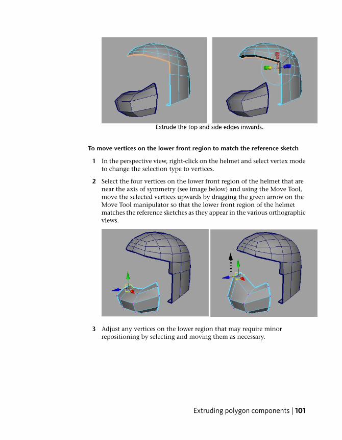
To move vertices on the lower front region to match the reference sketch
1 In the perspective view, right-click on the helmet and select vertex modeto change the selection type to vertices.
2 Select the four vertices on the lower front region of the helmet that arenear the axis of symmetry (see image below) and using the Move Tool,move the selected vertices upwards by dragging the green arrow on theMove Tool manipulator so that the lower front region of the helmetmatches the reference sketches as they appear in the various orthographicviews.
3 Adjust any vertices on the lower region that may require minorrepositioning by selecting and moving them as necessary.
Extruding polygon components | 101

Bridging between edgesNext you’ll connect the lower front region to the helmet mesh. You can createmeshes that bridge between one or more border edges of a mesh using theBridge feature (Edit Mesh > Bridge).
When using the bridge feature you must ensure that:
■ the edges to be bridged are in the same polygon mesh. That is, you mustcombine the two meshes into one using the Combine feature, before youperform the bridge.
■ you select an equal number of border edges on either side of the region tobe bridged.
To combine the two meshes into one
1 In the perspective view, right-click the mesh and select Object Mode fromthe marking menu that appears.
2 Select the helmet mesh, and then shift-select the lower front mesh, soboth meshes are selected.
3 Select Mesh > Combine.
The two meshes are combined into one. When you select either objectnow, the other is also selected because they are in the same mesh.
The edge of the mesh on the lower front region of the helmet is comprisedof five edges. The corresponding region on the side region of the helmet onlyhas three. You can increase the number of edges on the lower side region by
102 | Chapter 3 Polygonal Modeling
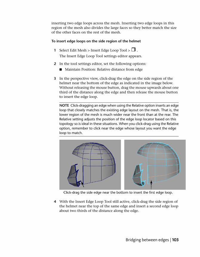
inserting two edge loops across the mesh. Inserting two edge loops in thisregion of the mesh also divides the large faces so they better match the sizeof the other faces on the rest of the mesh.
To insert edge loops on the side region of the helmet
1 Select Edit Mesh > Insert Edge Loop Tool > .
The Insert Edge Loop Tool settings editor appears.
2 In the tool settings editor, set the following options:
■ Maintain Position: Relative distance from edge
3 In the perspective view, click-drag the edge on the side region of thehelmet near the bottom of the edge as indicated in the image below.Without releasing the mouse button, drag the mouse upwards about onethird of the distance along the edge and then release the mouse buttonto insert the edge loop.
NOTE Click-dragging an edge when using the Relative option inserts an edgeloop that closely matches the existing edge layout on the mesh. That is, thelower region of the mesh is much wider near the front than at the rear. TheRelative setting adjusts the position of the edge loop locator based on thistopology so is ideal in these situations. When you click-drag using the Relativeoption, remember to click near the edge whose layout you want the edgeloop to match.
4 With the Insert Edge Loop Tool still active, click-drag the side region ofthe helmet near the top of the same edge and insert a second edge loopabout two thirds of the distance along the edge.
Bridging between edges | 103

5 Press the q key to return to selection mode, and click anywhere off themesh to unselect the edges.
Now that you’ve inserted the necessary edges, you can proceed withcreating the bridge.
To bridge between the lower front and side region of the helmet
1 Choose Select > Select Border Edge Tool and then click the border edgeson both the lower front as well as the side region of the mesh where youwant the bridging mesh to be constructed. (You should have five edgesselected on either side).
TIP When you select border edges using the Select Border Edge Tool youcan click on the first and last edge in a series on one side of the bridge andthe tool will select the edges in between.
104 | Chapter 3 Polygonal Modeling

2 Select Edit Mesh > Bridge > .
3 In the Bridge Options window, set the Divisions to 0, then click the Bridgebutton to create the bridge.
4 Press the q key to return to select mode, and click anywhere off the meshto unselect the edges.
NOTE If your bridge appears to twist or cross over itself it indicates that thetwo meshes have their surface normals mismatched. In this particular case itlikely indicates that you did not create the original profile shape for the lowerfront by placing the six vertices in a counter-clockwise direction.
If this occurs you must undo your steps to the point immediately before youcombined the two meshes and then reverse the surface normals on only thelower front section by selecting it and then selecting Normals > Reverse. Youcan then redo the instructions in this section as required.
Adding polygons to a meshFor the protective face shield on the helmet, you'll create one large multi-sidedpolygon using the Append to Polygon Tool and then split it into multiplefour-sided polygons (quads) so that the new polygons match the existingfour-sided topology of the helmet mesh.
To create the face shield using the Append to Polygon Tool
1 Tumble the perspective view so you can see all of the edges surroundingthe area for the face shield.
Adding polygons to a mesh | 105

2 Select Edit Mesh > Append to Polygon Tool > .
3 In the Append to Polygon Tool settings window, set the following:
■ Keep new faces planar: Off
If the planar option is on, the Append to Polygon Tool will not create amulti-sided polygon as the edges you’ll select do not form a planar region.
4 In the perspective view, click once on the top inner border edge of thehelmet mesh to indicate which mesh you are appending to, and thenclick the same edge a second time to begin the append operation (seeimage below).
5 Click the bottom edge of the face shield that is opposite the first edgeyou just clicked.
A polygon appears that spans the two edges.
6 Continue to click the remaining border edges in a counter-clockwisedirection around the opening for the face shield (see image above) untilyou reach the last edge.
7 When you are finished clicking the perimeter border edges for the faceshield, press the q key to quit the tool.
The multi-sided polygon is completed and added to the existing mesh.Multi-sided polygons are also referred to as n-gons.
106 | Chapter 3 Polygonal Modeling

Ideally, all faces should be four-sided to match the other faces on the helmetmesh. In the next section, you'll split the n-gon vertically and horizontallyinto several smaller four-sided polygons using the Split Polygon Tool.
Splitting polygon facesEarlier in the lesson you split the helmet mesh by inserting edge loops acrossthe mesh. You can split localized areas of a mesh using the Split Polygon Tool.When using the tool you draw a line across the faces to indicate the locationfor the split. You'll begin by vertically splitting the face shield.
To split the face shield vertically
1 Select Edit Mesh > Split Polygon Tool > .
The Split Polygon Tool settings editor appears.
2 Set the following options:
■ Split only from edges: On
■ Use snapping points along the edge: On
■ Snapping tolerance: 100
These settings let you begin and end your split at a location thatcorresponds exactly with an edge and lets you snap to the midpoint andends of the edge you select. (The number of points setting of 1 ensuresthis). These settings will help to ensure that the faces you split alignexactly and that the four-sided topology of the mesh is maintained.
Splitting polygon faces | 107

3 Tumble the camera in the perspective view so you can view both theupper inner edges of the face shield as well as the lower inner edges.
4 Click-drag the top inner edge of the face shield to indicate the start ofthe split (see image below). Drag the mouse to position the vertex untilit stops at the right side of the edge.
5 Click-drag on the lower inner edge of the helmet mesh to indicate theend of the split (see image). Drag the mouse to the right until the vertexstops at the right side of the edge.
6 Press the y key to split the face.
7 Press the g key to select the Split Polygon Tool again, and then continueto split the face shield vertically at the other locations specified in theimage below. Remember to press the y key after each split and then theg key to select the tool again.
When you are finished the n-gon for the face shield will be split into fouror five new polygons (depending on how you've constructed your mesh).
One polygon on the side of the face shield will still be five-sided. To correctthis, you'll also split the face shield horizontally. Splitting the face shieldhorizontally will also let you modify its shape afterwards.
108 | Chapter 3 Polygonal Modeling
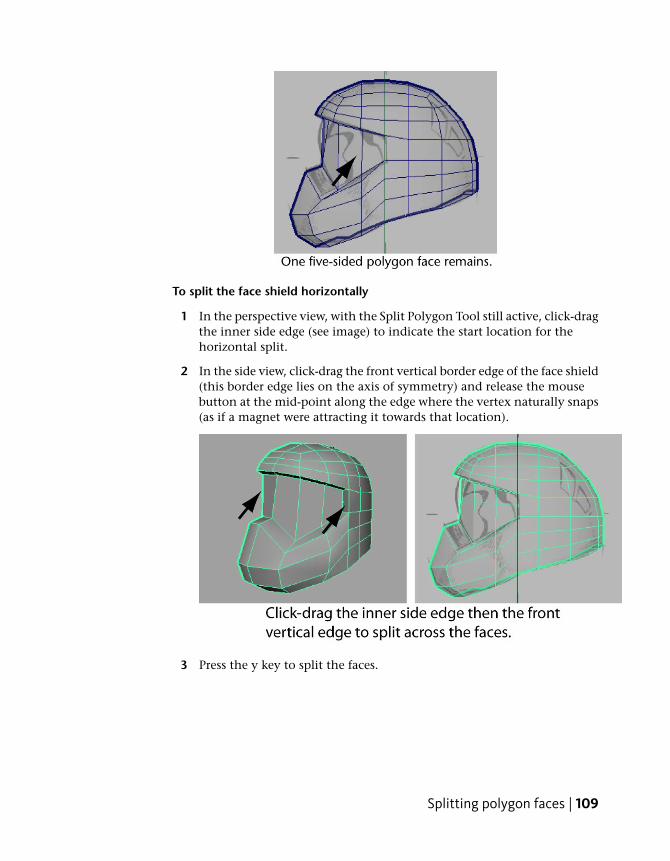
To split the face shield horizontally
1 In the perspective view, with the Split Polygon Tool still active, click-dragthe inner side edge (see image) to indicate the start location for thehorizontal split.
2 In the side view, click-drag the front vertical border edge of the face shield(this border edge lies on the axis of symmetry) and release the mousebutton at the mid-point along the edge where the vertex naturally snaps(as if a magnet were attracting it towards that location).
3 Press the y key to split the faces.
Splitting polygon faces | 109

NOTE When you split across multiple faces at the same time you only needto click an edge to indicate the start point for the split and on a second edgeto indicate the end point. The Split Polygon Tool automatically splits theedges in between.
4 Press the q key to quit the Split Polygon Tool.
In the next steps you'll reposition some of the vertices along the horizontalsplit to make the face shield protrude outwards a small amount.
To adjust the shape of the face shield
1 In the side view, select the middle two vertices at the front of the faceshield and use the Move Tool to move the vertices outwards (+Z) a smallamount (see image).
2 In the perspective view, select the remaining middle vertices on the faceshield one at a time and reposition them outwards a small distance usingthe Move Tool with the Move Setting option set to Normal.
110 | Chapter 3 Polygonal Modeling
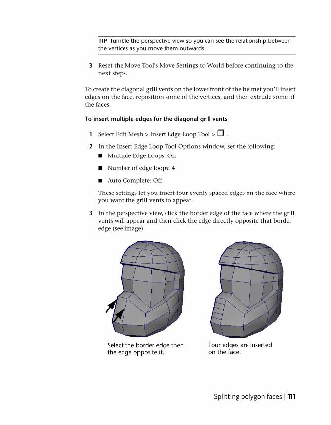
TIP Tumble the perspective view so you can see the relationship betweenthe vertices as you move them outwards.
3 Reset the Move Tool's Move Settings to World before continuing to thenext steps.
To create the diagonal grill vents on the lower front of the helmet you’ll insertedges on the face, reposition some of the vertices, and then extrude some ofthe faces.
To insert multiple edges for the diagonal grill vents
1 Select Edit Mesh > Insert Edge Loop Tool > .
2 In the Insert Edge Loop Tool Options window, set the following:
■ Multiple Edge Loops: On
■ Number of edge loops: 4
■ Auto Complete: Off
These settings let you insert four evenly spaced edges on the face whereyou want the grill vents to appear.
3 In the perspective view, click the border edge of the face where the grillvents will appear and then click the edge directly opposite that borderedge (see image).
Splitting polygon faces | 111
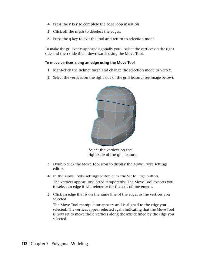
4 Press the y key to complete the edge loop insertion
5 Click off the mesh to deselect the edges.
6 Press the q key to exit the tool and return to selection mode.
To make the grill vents appear diagonally you’ll select the vertices on the rightside and then slide them downwards using the Move Tool.
To move vertices along an edge using the Move Tool
1 Right-click the helmet mesh and change the selection mode to Vertex.
2 Select the vertices on the right side of the grill feature (see image below).
3 Double-click the Move Tool icon to display the Move Tool’s settingseditor.
4 In the Move Tools’ settings editor, click the Set to Edge button.
The vertices appear unselected temporarily. The Move Tool expects youto select an edge it will reference for the axis of movement.
5 Click an edge that is on the same line of the edges as the vertices youselected.
The Move Tool manipulator appears and is aligned to the edge youselected. The vertices appear selected again indicating that the Move Toolis now set to move those vertices along the axis defined by the edge youselected.
112 | Chapter 3 Polygonal Modeling

6 Drag the red arrow on the Move manipulator downwards to move thevertices so that the shape of the faces for the grill are more diagonal (seeimage).
NOTE Make sure you do not move the vertices so that the lowest vertextouches the corner vertices or you’ll create an edge that has zero length.
7 Click off the mesh to deselect the vertices.
8 Before proceeding to the next section, double-click the Move Tool andreset the tool settings by clicking the Reset Tool button.
To make the grill vents three-dimensional, you’ll extrude some of the thindiagonal faces inwards.
To extrude the faces for the grill feature
1 Right-click the helmet mesh and change the selection mode to Face.
2 Beginning at the bottom of the grill feature, shift-select the two diagonalfaces as indicated in the image below.
Splitting polygon faces | 113
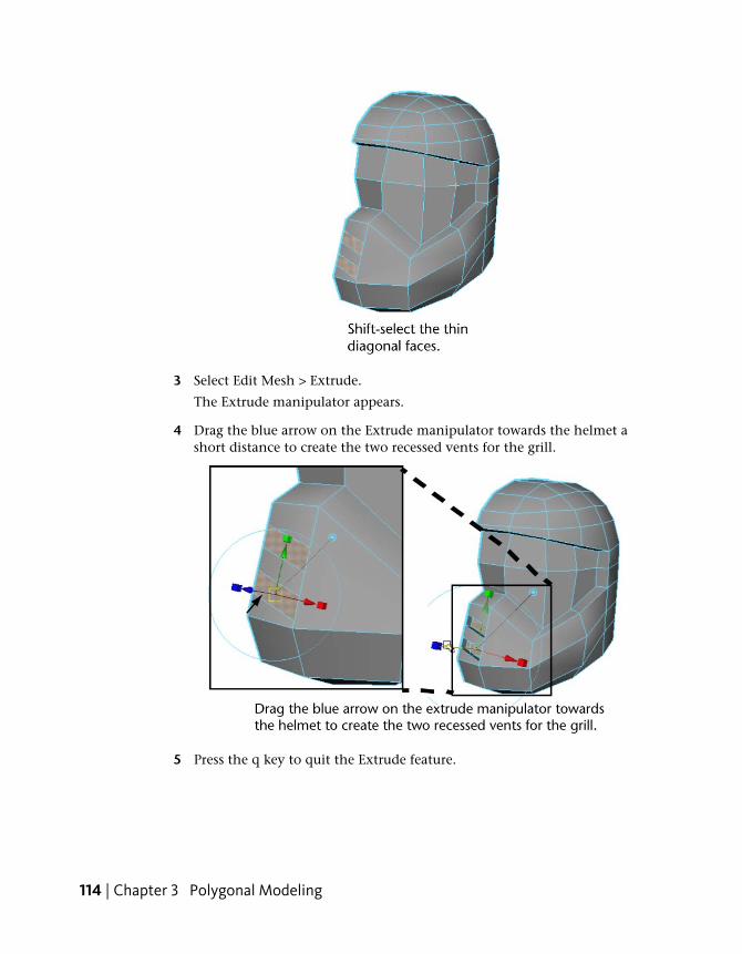
3 Select Edit Mesh > Extrude.
The Extrude manipulator appears.
4 Drag the blue arrow on the Extrude manipulator towards the helmet ashort distance to create the two recessed vents for the grill.
5 Press the q key to quit the Extrude feature.
114 | Chapter 3 Polygonal Modeling
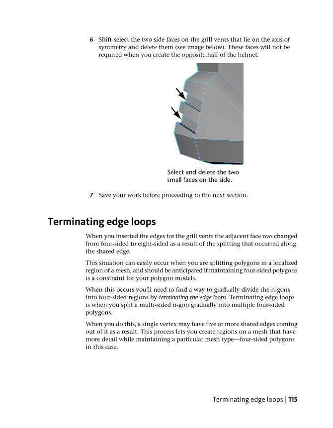
6 Shift-select the two side faces on the grill vents that lie on the axis ofsymmetry and delete them (see image below). These faces will not berequired when you create the opposite half of the helmet.
7 Save your work before proceeding to the next section.
Terminating edge loopsWhen you inserted the edges for the grill vents the adjacent face was changedfrom four-sided to eight-sided as a result of the splitting that occurred alongthe shared edge.
This situation can easily occur when you are splitting polygons in a localizedregion of a mesh, and should be anticipated if maintaining four-sided polygonsis a constraint for your polygon models.
When this occurs you’ll need to find a way to gradually divide the n-gonsinto four-sided regions by terminating the edge loops. Terminating edge loopsis when you split a multi-sided n-gon gradually into multiple four-sidedpolygons.
When you do this, a single vertex may have five or more shared edges comingout of it as a result. This process lets you create regions on a mesh that havemore detail while maintaining a particular mesh type—four-sided polygonsin this case.
Terminating edge loops | 115

To manually split the multi-sided polygon into three four-sided polygons
1 Select Edit Mesh > Split Polygon Tool.
2 In the perspective view, click-drag on the top side edge of the top grillvent. Drag your mouse so the vertex is positioned at the bottom of theedge (see image).
3 Click-drag on the top edge of the multi-sided polygon and slide the vertexto the right end of the edge (see image).
4 Press the y key to split the face.
The region above the split edge appears like a polygon but is actuallyfour-sided because of the edges on the grill vent.
5 Split the side edge on the bottom grill vent in a similar fashion byclick-dragging your mouse so the vertex is positioned at the top of theedge (see image below).
116 | Chapter 3 Polygonal Modeling

6 Click-drag the bottom edge of the multi-sided polygon and slide thevertex to the right end of the edge (see image).
7 Press the y key to split the face.
Your multi-sided face is now split into three four-sided faces, maintainingthe overall quad topology on the helmet mesh.
8 Press the q key to exit the Split Polygon Tool.
Deleting construction historyMaya keeps track of the options, attribute settings, and transformations madeto an object via its construction history. Construction history is useful whenyou’re working on a surface and want to edit an attribute from an earlier stageof the model’s development.
The simplest way to access the construction history for an object is via itsvarious input nodes in the Channel Box or via the Attribute Editor. Selectingan input node displays the attributes associated with that particularmodification to the object. You then edit the attributes on that node asrequired and the surface updates.
For example, the input nodes for the helmet mesh include: polyCreateFace,polyCube, polyExtrudeFace, polySmoothFace, polyMoveVertex, polyUnite,and so on. You can associate the steps in creating the helmet mesh with nodesthat are related to a particular stage of its construction history.
Deleting construction history | 117
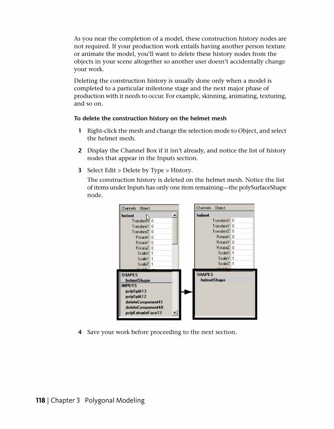
As you near the completion of a model, these construction history nodes arenot required. If your production work entails having another person textureor animate the model, you’ll want to delete these history nodes from theobjects in your scene altogether so another user doesn’t accidentally changeyour work.
Deleting the construction history is usually done only when a model iscompleted to a particular milestone stage and the next major phase ofproduction with it needs to occur. For example, skinning, animating, texturing,and so on.
To delete the construction history on the helmet mesh
1 Right-click the mesh and change the selection mode to Object, and selectthe helmet mesh.
2 Display the Channel Box if it isn’t already, and notice the list of historynodes that appear in the Inputs section.
3 Select Edit > Delete by Type > History.
The construction history is deleted on the helmet mesh. Notice the listof items under Inputs has only one item remaining—the polySurfaceShapenode.
4 Save your work before proceeding to the next section.
118 | Chapter 3 Polygonal Modeling

Mirror copying a meshOnce you’ve finalized one half of your polygon model (and deleted itsconstruction history) you’ll want to create the opposite half by copying itacross the axis of symmetry so you have the complete model. You can producea mirrored copy of a polygon mesh using Mirror Geometry (Mesh > MirrorGeometry).
Before copying one half across the axis of symmetry, you should check thatall of the border edges lie along the axis of symmetry. If any edges do not liealong this axis, the original half will be copied based on the vertices that createthe widest point and a gap between the two halves may result.
To ensure that the border vertices lie along the axis of symmetry
1 Enlarge the front view so you can view the vertices that lie along the axisof symmetry.
If any vertices on the mesh protrude across the Y axis, you’ll need to snapthese to the Y axis using the Move Tool in combination with the Snapto grids feature.
NOTE Any vertices that protrude across the Y axis likely occurred as a resultof an earlier extrude operation. Because the extrude feature extrudescomponents based on the face normal, a few vertices may have moved acrossthe axis of symmetry.
2 In the front view, select all of the vertices that should lie along the axisof symmetry (Y axis) using a bounding box selection.
3 On the Status Line, turn on Snap to Grids.
4 In the Toolbox, double-click the Move Tool to display its tool settingsand ensure that the Retain component spacing setting is turned off.
5 In the front view, click-drag the red arrow on the Move Tool manipulatorto the right a small distance.
The vertices immediately snap to the grid line to the right. They initiallywill not be positioned at the location you want, but you’ll notice that allof the vertices you selected are now aligned to each other.
6 Drag the manipulator towards the left until the vertices snap to the Yaxis.
Mirror copying a mesh | 119
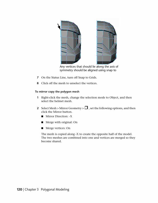
7 On the Status Line, turn off Snap to Grids.
8 Click off the mesh to unselect the vertices.
To mirror copy the polygon mesh
1 Right-click the mesh, change the selection mode to Object, and thenselect the helmet mesh.
2 Select Mesh > Mirror Geometry > , set the following options, and thenclick the Mirror button.
■ Mirror Direction: -X
■ Merge with original: On
■ Merge vertices: On
The mesh is copied along -X to create the opposite half of the model.The two meshes are combined into one and vertices are merged so theybecome shared.
120 | Chapter 3 Polygonal Modeling

3 Save your work before proceeding to the next section.
At this point, the low resolution version of the helmet model is complete. Inthe next section you’ll preview how the model appears at a higher resolutionusing the subdiv proxy feature.
Working with a smoothed meshDepending on the intended use of your polygonal model, you may want alow resolution version, a high resolution version, or both. In Maya, its easyto increase the resolution of a model using the Smooth feature (Mesh >Smooth).
In addition, you can preview a higher resolution version of the mesh usingeither Smooth Mesh Preview or the Proxy > Subdiv Proxy feature. You canthen view and edit the low resolution and high resolution smoothed versionof the mesh separately or simultaneously.
Smooth Mesh Preview lets you quickly preview how your mesh will appearwhen smoothed.
The Subdiv Proxy feature links the original and the high resolution smoothedversions via construction history, you can make changes to the low resolutionversion and immediately see the effect on the high resolution smoothedversion.
In this lesson, you’ll use Subdiv Proxy to work with your smoothed mesh.
Working with a smoothed mesh | 121

To create a high resolution smoothed model using Subdiv Proxy
1 Right-click the mesh, change the selection mode to Object, and thenselect the helmet mesh.
2 Select Proxy > Subdiv Proxy > , and set the following:
■ Division Levels: 2
■ Mirror Behavior: None
■ Subdiv Proxy Shader: Keep
3 Click the Smooth button.
A higher resolution, smoothed copy of the helmet mesh is created in thesame position as the original mesh. It is possible to see the two versionsin this position (and you can toggle the display to show either or both)but in this lesson you’ll select the high resolution version and move itslightly to the left.
NOTE The two versions of the model are also grouped into the same nodehierarchy when the Subdiv Proxy operation is performed.
4 Select both the low and high resolution versions of the mesh in ObjectMode.
122 | Chapter 3 Polygonal Modeling

5 Press the ‘ key (located to the left of the 1 key) to toggle the displaybetween the low and high resolution versions.
Toggling the display between the two versions is useful when you wantto view one or the other.
6 Press the ~ key to toggle the display so that both are visible again.
NOTE The Toggle Proxy Display (‘) and the Both Proxy and Subdiv Display(~) display items are also available from within the Proxy menu.
7 Select only the smoothed version of the mesh in Object Mode and moveit to the left about 25 units (X = -25).
As you edit the low resolution version of the helmet mesh you’ll see theresulting updates on the smoothed version beside it.
Creasing and hardening edges on a meshYou can crease or harden the edges on your polygon meshes. Hardening orcreasing the edges sets how the mesh transitions between faces enhancingthe realism of your model.
When you harden an edge on a polygon mesh, you change the direction ofthe normals associated with the shared edge, which in turn affects the shadingalong those edges. When you crease an edge of a mesh that has an associatedsubdiv proxy, the edges on the smoothed high resolution version are creasedby physically modifying the polygon smoothing surrounding those edges.
Creasing and hardening edges on a mesh | 123

In this lesson, you’ll try both methods on your helmet mesh.
To display hard and soft edges on a mesh
1 Right-click the low resolution mesh, set the selection type to Object Mode,and then select the helmet mesh.
2 Select Soft/Hard Edges.
The wireframe mesh on the helmet updates to display both dashed andsolid lines. The dashed lines indicate edges that are set to display as softshaded. The solid lines indicate edges that are set to display as hardshaded. The reason some of the edges are hard and some are soft relatesto the particular settings for some polygon tools.
To soften the edges on the mesh
➤ With the low resolution version of the helmet still selected, select Normals> Soften Edge.
All of the edges on the helmet mesh are set to be shaded in a softened fashion.The wireframe mesh updates to display as dashed lines indicating that all ofthe edges are set to be soft shaded. You may not notice any immediate effecton the smoothed high resolution version, but its important that you performthis step before you proceed to harden specific edges on this model.
124 | Chapter 3 Polygonal Modeling

To harden the edges surrounding the face shield
1 Right-click the low resolution mesh and set the selection mode to Edge.
2 Select the inner edges that surround the perimeter of the face shield (seeimage below).
TIP You can quickly select the inner edges surrounding the perimeter of theface shield using the Select Edge Loop Tool. You may need to double-clickin a couple of areas to complete the selection.
3 Select Normals > Harden Edge.
The selected edges are hardened on the low resolution mesh.
Creasing and hardening edges on a mesh | 125
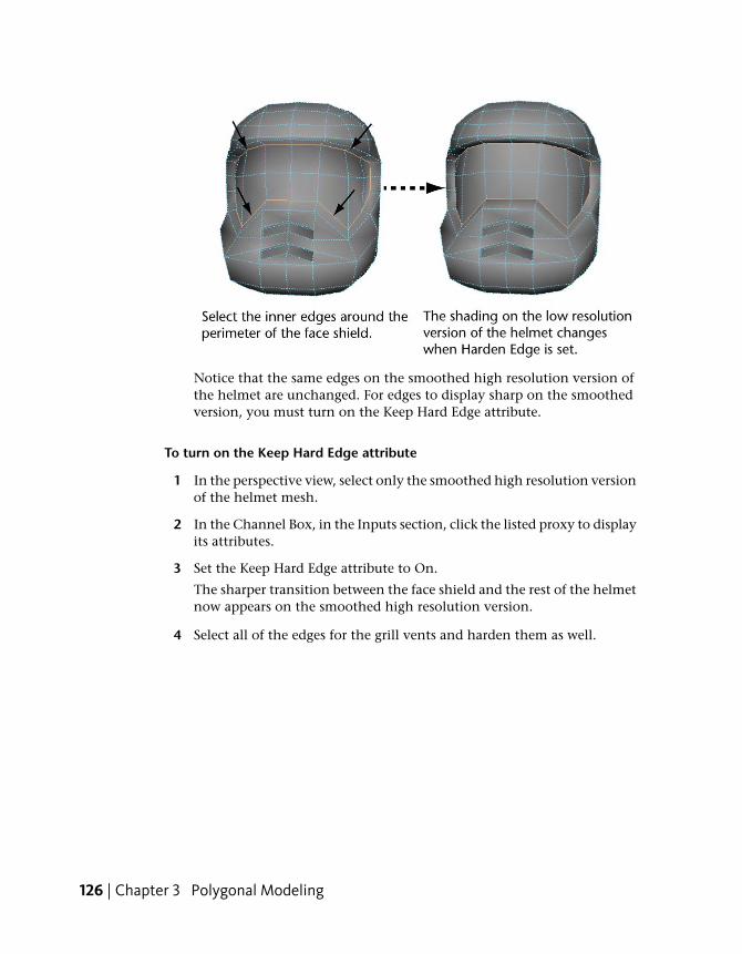
Notice that the same edges on the smoothed high resolution version ofthe helmet are unchanged. For edges to display sharp on the smoothedversion, you must turn on the Keep Hard Edge attribute.
To turn on the Keep Hard Edge attribute
1 In the perspective view, select only the smoothed high resolution versionof the helmet mesh.
2 In the Channel Box, in the Inputs section, click the listed proxy to displayits attributes.
3 Set the Keep Hard Edge attribute to On.
The sharper transition between the face shield and the rest of the helmetnow appears on the smoothed high resolution version.
4 Select all of the edges for the grill vents and harden them as well.
126 | Chapter 3 Polygonal Modeling
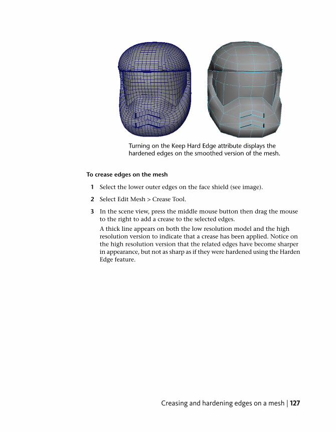
To crease edges on the mesh
1 Select the lower outer edges on the face shield (see image).
2 Select Edit Mesh > Crease Tool.
3 In the scene view, press the middle mouse button then drag the mouseto the right to add a crease to the selected edges.
A thick line appears on both the low resolution model and the highresolution version to indicate that a crease has been applied. Notice onthe high resolution version that the related edges have become sharperin appearance, but not as sharp as if they were hardened using the HardenEdge feature.
Creasing and hardening edges on a mesh | 127

4 Save your work.
NOTE You can toggle the creased edge display (thick lines) by selectingCrease Edges.
Your model is now complete. Depending on your requirements you can deletethe construction history on both the low resolution and high resolutionversions.
Refine any regions on the helmet as required to gain more experience withthe tools presented in this lesson.
If you need to work with either version of the model separately you canungroup the two meshes by selecting the top node of their hierarchy in the
128 | Chapter 3 Polygonal Modeling
Hypergraph window (Window > Hypergraph: Hierarchy) and selecting Edit >Ungroup.
Beyond the lessonIn this lesson you learned some basic techniques of polygonal modeling:
■ You can create complex polygonal models with surprisingly few techniques.
■ Starting from a primitive surface such as a cube, you can smooth, scale,move, extrude, split, and rotate components of the primitive to create alow resolution version of the model you want to create.
■ You must frequently adjust vertices to fine-tune the shape, and finallysmooth the edges between faces where desired in order to produce thefinal version of your model.
■ Another method for previewing a smoothed version of the mesh before itis smoothed is via Smooth Mesh Preview. Press the 2 or 3 key while themesh is selected to preview it in a smoothed state. Press the 1 key to returnit to the unsmoothed state.
Polygonal modeling has many timesaving features not covered in this lesson:
■ For example, Boolean operations (union, difference, and intersection) area common way to create a new object from the interaction of two existingobjects.
■ If you’re planning to use your polygonal surfaces where the poly count isconstrained, such as with interactive games, Maya has a number of toolsfor minimizing the number of polygonal faces of an object such as theReduce Tool. Fewer faces means simpler geometry. This is critical whenfewer polygons means increased interactive performance with gamesapplications. You can view the polygon count on your mesh by selectingthe mesh and then choosing Poly Count.
■ Maya also has a category of tools called Deformers. Deformers let you bend,twist, and scale your objects by enveloping the object in a cage-likemanipulator called a lattice deformer that you can manipulate.
■ The NURBS chapter in this guide describes how to use the Sculpt GeometryTool to modify a surface by pushing, pulling, and smoothing a surfacewithout first selecting vertices. Though the lesson shows how to shape aNURBS surface, you can apply many of the same techniques when sculptingpolygonal surfaces.
Beyond the lesson | 129
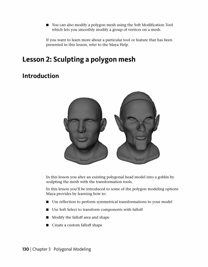
■ You can also modify a polygon mesh using the Soft Modification Toolwhich lets you smoothly modify a group of vertices on a mesh.
If you want to learn more about a particular tool or feature that has beenpresented in this lesson, refer to the Maya Help.
Lesson 2: Sculpting a polygon mesh
Introduction
In this lesson you alter an existing polygonal head model into a goblin bysculpting the mesh with the transformation tools.
In this lesson you’ll be introduced to some of the polygon modeling optionsMaya provides by learning how to:
■ Use reflection to perform symmetrical transformations to your model
■ Use Soft Select to transform components with falloff
■ Modify the falloff area and shape
■ Create a custom falloff shape
130 | Chapter 3 Polygonal Modeling

■ Select components using Marquee select and Drag select
■ Use Camera based selection to limit the components you select
■ Use the Split Edge Tool to separate edge rings
Open the scene for the lessonIn this lesson, you’ll work with a scene that we created for your use. The scenecontains a human head. In the remainder of the lesson, you’ll alter this intoa goblin head.
To open the scene
1 Make sure you’ve done the steps in Preparing for the lesson on page 72.
2 Open the scene file named Poly_head.mb.
This file can be found in the Getting Started directory that you set asyour Maya project:
Getting Started/PolygonModeling/Poly_head.mb
The scene contains a human head in a visible layer with a hat and glasseson hidden layers.
Using Soft SelectYou can use Soft Select to select components with falloff on a polygon orNURBS surface. Falloff is an area around the selected components that isaffected by a transformation according to a weighting. Transformingcomponents with falloff allows you to perform a smooth transformation overmultiple components without having to adjust each component individually.
For this lesson you use Soft Select to make a number of adjustments to thehead model, starting with the nose.
To stretch the nose
1 Select the Move Tool by clicking the icon on the Toolbox.
2 Right-click the head model and select Vertex from the marking menu.
The vertices appear on the mesh.
3 Select a vertex on the tip of the nose.
Open the scene for the lesson | 131
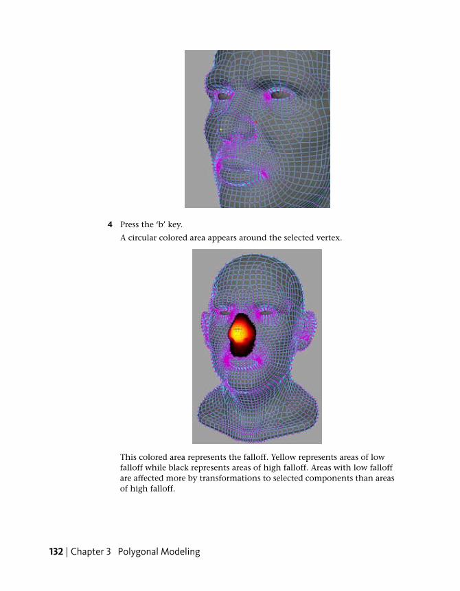
4 Press the ‘b’ key.
A circular colored area appears around the selected vertex.
This colored area represents the falloff. Yellow represents areas of lowfalloff while black represents areas of high falloff. Areas with low falloffare affected more by transformations to selected components than areasof high falloff.
132 | Chapter 3 Polygonal Modeling

Next you need to adjust the Falloff radius.
5 Hold the b key and drag the left mouse button left or right.
The falloff area grows and shrinks as you move the mouse. Adjust thesize so that it encompasses as much of the nose as possible withouttouching the face.
6 Drag the z axis manipulator away from the face.
As you drag the vertex away, the rest of the nose is smoothly stretchedwith it.
Using Soft Select | 133
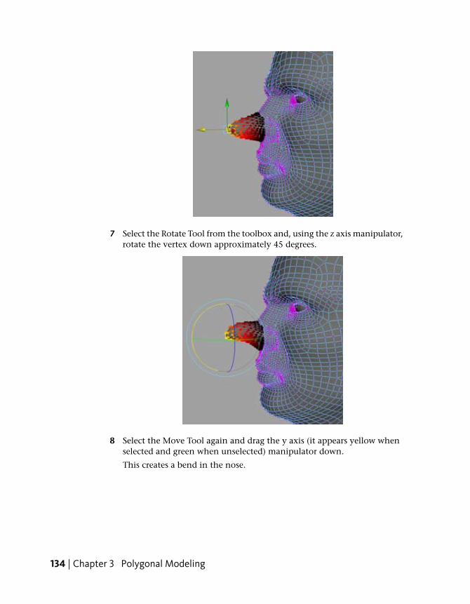
7 Select the Rotate Tool from the toolbox and, using the z axis manipulator,rotate the vertex down approximately 45 degrees.
8 Select the Move Tool again and drag the y axis (it appears yellow whenselected and green when unselected) manipulator down.
This creates a bend in the nose.
134 | Chapter 3 Polygonal Modeling

9 Turn off Soft Select by pressing the b key on your keyboard.
Selecting with Camera based selectionWhen selecting components on a model you often only want to select thecomponents you can see and not the components behind them. You can useCamera based selection to limit your marquee select to only what the cameracan see.
To pull out the chin
1 Double-click the Select Tool icon in the toolbox.
The Tool Settings editor appears.
2 In the Common Selection Options section, underneath Marquee, turnon Camera based selection.
3 Right-click the head and select Vertex from the marking menu.
The vertices appear on the mesh.
Selecting with Camera based selection | 135

4 While looking at the front of the head, select the five vertices on thesame vertex loop at the front of the chin by holding the left mouse buttonat one corner of them dragging a marquee selection over them.
Only the five vertices in the front are selected.
5 Turn on Soft Select by pressing the ‘b’ key on your keyboard.
A colored falloff appears on the surface of the face.
6 Hold the ‘b’ key on your keyboard and drag the the left mouse buttonleft or right to adjust the Falloff radius so that it encompasses only thechin.
7 Select the Move Tool and drag the chin down and away from the face sothat it becomes longer and more angular.
136 | Chapter 3 Polygonal Modeling

Now you have a longer chin without affecting any of the geometry on theneck, which may have occurred accidentally if Camera based selection hadbeen off.
Sculpting with symmetryTo give the head a more goblin-like appearance, you need to make the cheeksand eyebrows more boney. However, to do this, you need to adjust both cheeksequally. You can do this with the transformation tools’ Reflection settings.
To modify both cheeks simultaneously
1 Double-click the Move Tool in the Toolbox.
2 In the Reflection section, turn on Reflection and set the Reflection axisto X.
3 Right-click the head and select Vertex from the marking menu.
The vertices appear on the mesh.
Sculpting with symmetry | 137

4 With the camera positioned in front of the head, select a set of verticeson the left cheek.
A colored falloff appears on both cheeks.
5 Pull the x axis manipulator to the left so that the cheeks are pulled closertogether.
Both cheeks are transformed identically and appear more boney.
138 | Chapter 3 Polygonal Modeling

Now you can adjust the eyebrows to make the goblin angrier.
To rotate the eyebrows
1 Press the ‘b’ key on your keyboard to disable Soft Select.
2 Click the outermost vertex on the left eyebrow.
3 Shift + double-click the innermost vertex on the left eyebrow.
All the vertices on the same loop are selected between and including thetwo vertices.
Sculpting with symmetry | 139

NOTE The selection of vertices on the other side of the reflection seam donot appear complete after this step. This is normal and is rectified in step 4.
4 Press the ‘b’ key on your keyboard to enable Soft Select.
5 Hold the ‘b’ key on your keyboard and drag the mouse left and right toadjust the Falloff radius so that it only affects the eyebrow.
6 Double-click the Rotate Tool from the Toolbox.
The Tool Settings editor appears.
7 Drag the Z (dark blue) rotate manipulator in the scene to rotate theeyebrows inward.
140 | Chapter 3 Polygonal Modeling
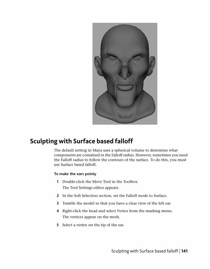
Sculpting with Surface based falloffThe default setting in Maya uses a spherical volume to determine whatcomponents are contained in the Falloff radius. However, sometimes you needthe Falloff radius to follow the contours of the surface. To do this, you mustuse Surface based falloff.
To make the ears pointy
1 Double-click the Move Tool in the Toolbox.
The Tool Settings editor appears.
2 In the Soft Selection section, set the Falloff mode to Surface.
3 Tumble the model so that you have a clear view of the left ear.
4 Right-click the head and select Vertex from the marking menu.
The vertices appear on the mesh.
5 Select a vertex on the tip of the ear.
Sculpting with Surface based falloff | 141

6 Hold the ‘b’ key on your keyboard and drag the mouse left or right toadjust the Falloff radius so that it encompasses the top half of the ear.
7 Use the manipulators to pull the ear until it’s pointed.
Surface based falloff ensures that only the ear is affected by yourtransformation. If you were using Volume based falloff, parts of the headwould also be moved along with the ear.
142 | Chapter 3 Polygonal Modeling

8 Select the Scale Tool and scale the ears along the x axis so they becomethinner.
9 Select the Move Tool again and pull the pointy end of the ears away fromthe head.
Selecting with Drag selectIn addition to marquee selecting sets of components, you can also select themby dragging over them with the mouse. This is similar to the way that thePaint Selection Tool works.
To make the eyes sockets more pronounced
1 Double-click the Select Tool in the Toolbox.
The Tool Settings editor appears.
2 In the Common Selection Options section, turn on Drag.
The mouse cursor turns into a brush cursor.
3 Beneath the Drag option, turn on Camera based selection.
4 Right-click the head and select Vertex from the marking menu.
Selecting with Drag select | 143

The vertices appear on the mesh.
5 On one side of the mesh, drag the mouse around the eye socket, beneaththe eyebrow until you’ve covered a small area around the eye.
You may find it easier to temporarily disable Soft Select to get a betterview of what you are selecting. You can quickly toggle Soft Select on andoff by pressing the ‘b’ key on your keyboard.
6 With Soft Select on, hold the ‘b’ key and drag the mouse to resize thefalloff area so it covers only the eye sockets.
7 Select the Move Tool in the Toolbox and pull the z axis manipulatortoward the head.
144 | Chapter 3 Polygonal Modeling
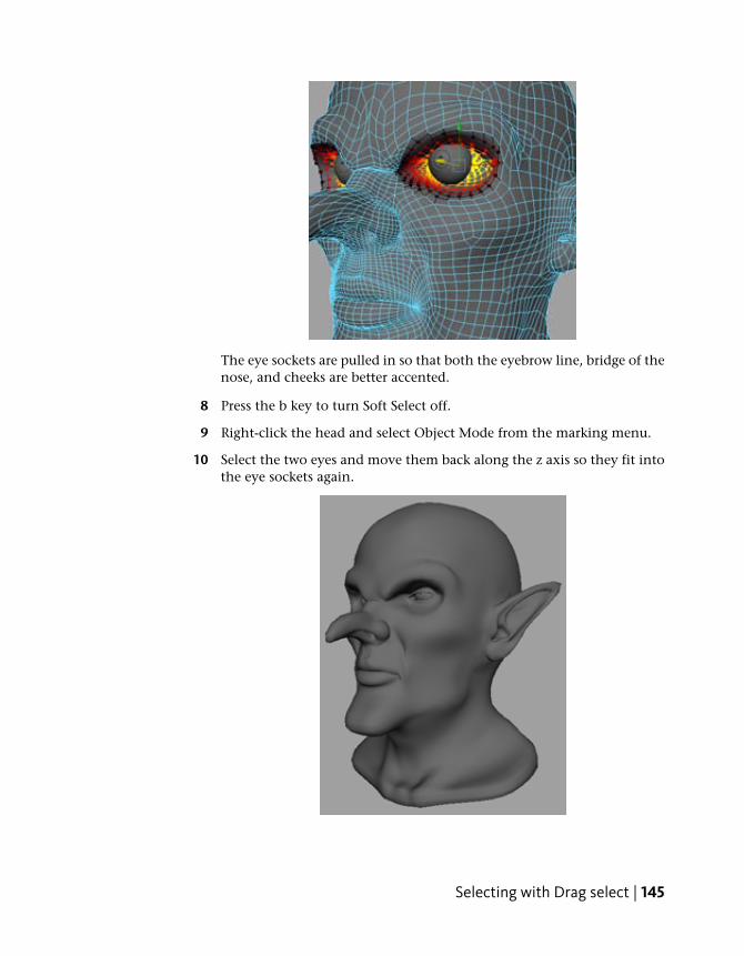
The eye sockets are pulled in so that both the eyebrow line, bridge of thenose, and cheeks are better accented.
8 Press the b key to turn Soft Select off.
9 Right-click the head and select Object Mode from the marking menu.
10 Select the two eyes and move them back along the z axis so they fit intothe eye sockets again.
Selecting with Drag select | 145

11 Set the selection mode back to Marquee.
Adjusting the Seam toleranceYou can use the seam tolerance to fatten the nose at the end.
1 Right-click the head and select Vertex from the marking menu.
The vertices appear on the mesh.
2 Select a vertex on the left side of the tip of the nose.
3 Press the ‘b’ key to turn Soft Select on.
4 Hold the ‘b’ key and move the mouse left or right to resize the Falloffradius so it only encompasses the tip of the nose.
5 Select the Move Tool by double-clicking it in the Toolbox.
6 In the Tool Settings Editor, in the Reflection Settings section, click theReset button.
7 Set the Seam Tolerance to 5.
The Seam Tolerance controls the falloff around the seam. By increasingthe number, you ensure that the vertices at the tip of the nose spreadevenly.
8 Move the vertex away from the reflection line along the x axis to widenthe end of the nose.
Now you can unhide the hat layer to finish off the goblin.
146 | Chapter 3 Polygonal Modeling

To unhide the hat
➤ Open the Channel Box and click the first empty box in the hat layer.
Beyond the lessonIn this lesson, you learned how to:
■ Activate Soft Select and adjust the Falloff radius.
■ Transform components with Soft Selection.
■ Use Camera based selection.
■ Select components using reflection.
■ Use both surface based and volume based falloff.
■ Use Drag select.
■ Adjust the Seam tolerance.
Beyond the lesson | 147
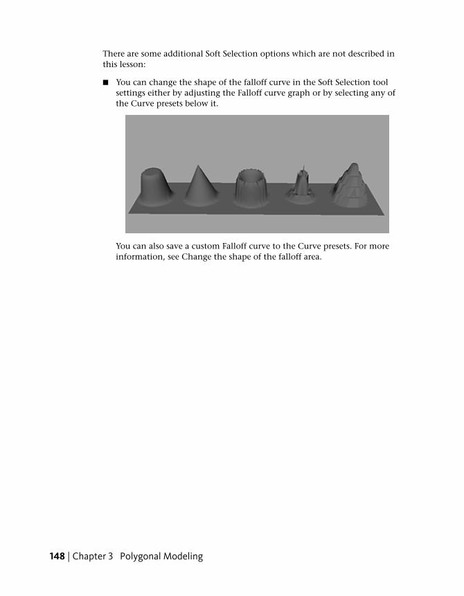
There are some additional Soft Selection options which are not described inthis lesson:
■ You can change the shape of the falloff curve in the Soft Selection toolsettings either by adjusting the Falloff curve graph or by selecting any ofthe Curve presets below it.
You can also save a custom Falloff curve to the Curve presets. For moreinformation, see Change the shape of the falloff area.
148 | Chapter 3 Polygonal Modeling

NURBS Modeling
IntroductionNURBS (Non-Uniform Rational B-splines) use a method of mathematicallydescribing curves and surfaces that are well suited to 3D applications. NURBSare characterized by the smooth organic forms they produce.
NURBS surfaces can be quickly modeled and edited using a variety of techniques.NURBS surfaces are created using one or more NURBS curves that define theprofile of the shape that you want for a surface, and then using a specificconstruction method to create the finished surface.
NURBS curves and surfaces have many applications and are the preferred surfacetype for industrial and automotive designers where smooth forms with minimaldata are required to define a particular form. NURBS curves are ideal for defininga smooth motion path for an animated object. With NURBS, a surface can bemodeled and then converted to a poly mesh.
In this chapter, you will learn some basic techniques for working with NURBScurves and surfaces in Maya. This chapter includes these lessons:
■ Lesson 1 Revolving a curve to create a surface: Introduction on page 150
■ Lesson 2 Sculpting a NURBS surface: Introduction on page 156
■ Lesson 3 Lofting curves to create a surface: Introduction on page 171
Preparing for the lessonsTo ensure the lessons work as described, do these steps before beginning:
1 Select File > New Scene to create a new scene before starting each lesson.
4
149

2 Make sure the Construction History icon (below the menu bar) is on:
. (If it is turned off, it has a large X across it.)
3 If you have not already done so, copy the GettingStarted folder fromits installation location to your projects directory. Then, set theGettingStarted directory as your Maya project. For more information,see Copying and setting the Maya project on page 25.
4 Select the Surfaces menu set. Unless otherwise noted, the directions inthis chapter for making menu selections assume you’ve already selectedthe Surfaces menu set.
NOTE Before you perform the lessons in this book, ensure that the InteractiveCreation option for primitives is turned off by selecting Create > NURBSPrimitives > Interactive Creation. That is, ensure a check mark does not appearbeside the menu item.
5 Make sure that Soft Selection is turned off by opening the Attribute Editorwith the Select Tool active and unchecking the box marked Soft Select.
Lesson 1: Revolving a curve to create a surface
Introduction
A simple technique for creating NURBS surfaces is to create a curve for theprofile of your desired form and then create a surface using one of the variousNURBS surfacing tools available in Maya. In this lesson, you create an eggholder using NURBS curves and the Revolve Tool.
150 | Chapter 4 NURBS Modeling
In this lesson you learn how to:
■ Create a NURBS curve using the control vertices (CV) creation technique.
■ Use the grid for visual reference when modeling.
■ Determine the start and end points for a NURBS curve and its direction.
■ Create a revolved NURBS surface using the Revolve tool.
■ Change the display shading smoothness for a NURBS surface.
■ Edit a NURBS surface by editing its initial profile curve when it is linkedto the surface by construction history.
Creating a profile curveRevolve is a common modeling technique similar to shaping a vase on aspinning potter’s wheel. You must first create a profile curve in an orthographicview and use the Revolve Tool to create a surface.
To create a profile curve
1 Make sure you’ve done the steps in Preparing for the lessons on page 149.
2 Select Panels > Layouts > Four Panes so you can see multiple views of thescene.
3 Select Create > CV Curve Tool.
This is the most commonly used tool for drawing curves.
Creating a profile curve | 151

4 In the front view, click the numbered positions as shown in the figure.Make sure the first and last positions are on the grid’s Y-axis (the thickestvertical line of the front view’s grid).
Also, click three times in the same spot for positions 9, 10, and 11. Thisis necessary to create a sharp point or corner in the curve.
To change the position of the most recent point clicked, you canmiddle-mouse drag it.
5 (Windows and Linux) After you click position 13, press Enter to completethe curve’s creation.
(Mac OS X) Press Return to complete the curve’s creation.
The points you clicked in the scene view become the control vertices(CVs) of the completed curve. CVs are points you manipulate to alter theshape of a curve (or surface). These points often lie away from the curve.
It takes a little practice to be able to predict exactly where a curve will bepositioned when you click CV positions with the CV Curve Tool. Onceyou’ve learned the technique, you’ll be able to create and edit curves withgraceful symmetry. By default, you must click at least four points to createa curve with the CV Curve Tool.
For some advanced operations in Maya, you need to know the meaningof the start of a curve and the curve direction. The start of a curve is the firstCV you create when you draw the curve. It is indicated by a small hollow
152 | Chapter 4 NURBS Modeling
box at the first CV, visible as you create the curve. Curve direction isshown on the second CV after the start of the curve, indicated by a smallu icon as you create the curve.
Creating a revolve surfaceWith the Revolve surface tool, a curve is rotated about an axis to create asurface. The user can define the axis of revolution.
To create a revolve surface
1 With the curve selected, select Surfaces > Revolve. This creates the eggholder surface from the revolved profile curve. Examine the results inthe perspective view.
Maya does not delete the profile curve. In a subsequent step, you’ll editthe profile curve to alter the shape of the surface.
2 Select the surface and rename it Eggholder in the Channel Box.
3 With the pointer in the perspective view, press 5 (for Shading > SmoothShade All).
This displays the egg holder as a shaded surface rather than a wireframein the perspective view.
Press 1, 2, and 3 to switch between the different degrees of displaysmoothness. (These hotkeys correspond to the menu items under Display> NURBS menu item (Rough/Medium/Fine).
The finer the smoothness, the greater the impact is on interactiveperformance when you work with complex models.
The smoothness display only affects the scene view. Rendered imagesdisplay with high quality smoothness regardless of this setting.
Editing a revolve surfaceAfter you create a surface from a revolved curve, you can reshape the originalcreation curve to reshape the surface. This is possible because Maya’sConstruction History feature was turned on before you did the revolveoperation.
Selecting the original creation curve can be challenging when it is situatedamongst other existing curves and surfaces. The Outliner is an editor that is
Creating a revolve surface | 153
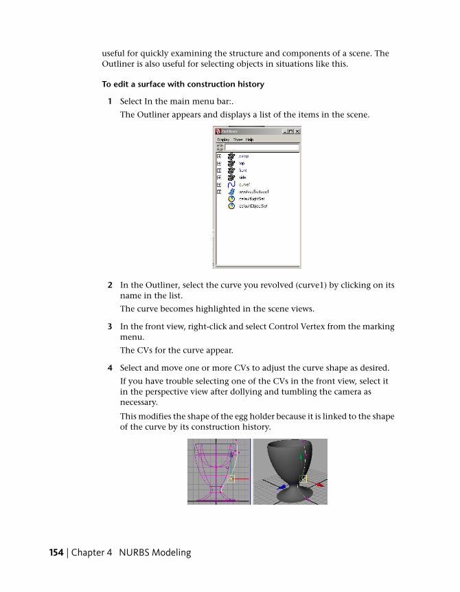
useful for quickly examining the structure and components of a scene. TheOutliner is also useful for selecting objects in situations like this.
To edit a surface with construction history
1 Select In the main menu bar:.
The Outliner appears and displays a list of the items in the scene.
2 In the Outliner, select the curve you revolved (curve1) by clicking on itsname in the list.
The curve becomes highlighted in the scene views.
3 In the front view, right-click and select Control Vertex from the markingmenu.
The CVs for the curve appear.
4 Select and move one or more CVs to adjust the curve shape as desired.
If you have trouble selecting one of the CVs in the front view, select itin the perspective view after dollying and tumbling the camera asnecessary.
This modifies the shape of the egg holder because it is linked to the shapeof the curve by its construction history.
154 | Chapter 4 NURBS Modeling

5 If desired, save the scene for future review.
6 Close the Outliner window.
Beyond the lessonIn this lesson you were introduced to a few basic techniques related to NURBSmodeling:
■ Revolving a curve is the easiest way to create surfaces with radiallysymmetrical forms— wheels, vases, glasses, pillars, and so on.
■ NURBS surfaces are webs of interconnected curves. The creation curves areused to create and subsequently modify the surfaces if required.
■ Proficiency at drawing and editing curves is an important part of NURBSmodeling.
■ The grid is a useful aid for constructing and modifying curves.
Some additional points you should know are:
■ You cannot render curves, so your work with them is always an adjunctto creating and editing surfaces.
■ Besides moving a curve’s CVs to alter its shape, you can cut, attach, extend,close, and smooth curves.
■ After you create a surface from a revolved curve, you can edit the surfaceat a component level by moving CVs or scaling groups of CVs on thatsurface to customize the shape of the surface. (You will need to turn offconstruction history in order to do this.)
Beyond the lesson | 155
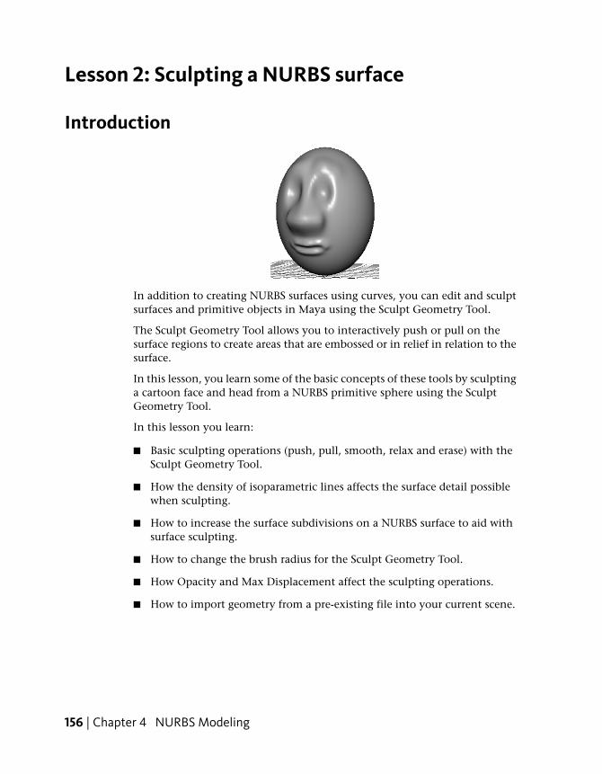
Lesson 2: Sculpting a NURBS surface
Introduction
In addition to creating NURBS surfaces using curves, you can edit and sculptsurfaces and primitive objects in Maya using the Sculpt Geometry Tool.
The Sculpt Geometry Tool allows you to interactively push or pull on thesurface regions to create areas that are embossed or in relief in relation to thesurface.
In this lesson, you learn some of the basic concepts of these tools by sculptinga cartoon face and head from a NURBS primitive sphere using the SculptGeometry Tool.
In this lesson you learn:
■ Basic sculpting operations (push, pull, smooth, relax and erase) with theSculpt Geometry Tool.
■ How the density of isoparametric lines affects the surface detail possiblewhen sculpting.
■ How to increase the surface subdivisions on a NURBS surface to aid withsurface sculpting.
■ How to change the brush radius for the Sculpt Geometry Tool.
■ How Opacity and Max Displacement affect the sculpting operations.
■ How to import geometry from a pre-existing file into your current scene.
156 | Chapter 4 NURBS Modeling
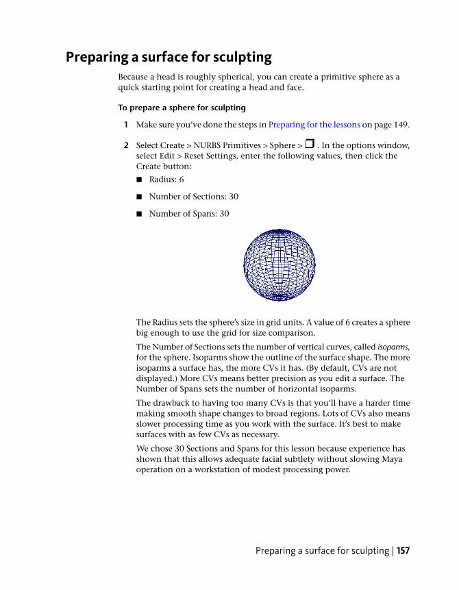
Preparing a surface for sculptingBecause a head is roughly spherical, you can create a primitive sphere as aquick starting point for creating a head and face.
To prepare a sphere for sculpting
1 Make sure you’ve done the steps in Preparing for the lessons on page 149.
2 Select Create > NURBS Primitives > Sphere > . In the options window,select Edit > Reset Settings, enter the following values, then click theCreate button:
■ Radius: 6
■ Number of Sections: 30
■ Number of Spans: 30
The Radius sets the sphere’s size in grid units. A value of 6 creates a spherebig enough to use the grid for size comparison.
The Number of Sections sets the number of vertical curves, called isoparms,for the sphere. Isoparms show the outline of the surface shape. The moreisoparms a surface has, the more CVs it has. (By default, CVs are notdisplayed.) More CVs means better precision as you edit a surface. TheNumber of Spans sets the number of horizontal isoparms.
The drawback to having too many CVs is that you’ll have a harder timemaking smooth shape changes to broad regions. Lots of CVs also meansslower processing time as you work with the surface. It’s best to makesurfaces with as few CVs as necessary.
We chose 30 Sections and Spans for this lesson because experience hasshown that this allows adequate facial subtlety without slowing Mayaoperation on a workstation of modest processing power.
Preparing a surface for sculpting | 157

NOTE In wireframe display mode, if you select Display > NURBS > Fine orMedium, more isoparms appear than there are actual spans and sections.The surface is visually displayed with extra precision, but the extra isoparmshave no CVs and cannot be edited.
3 Name the sphere Egghead.
4 Rotate the sphere 90 degrees on its side (Rotate Z: 90). This positions thesphere’s CVs well for modeling a simple head and face. You’ll learn whylater in this lesson.
5 To give Egghead an oval shape, set the ScaleX for the sphere to 1.3 or so.Optionally, you can move Egghead above the grid so the grid doesn’tinterfere with your view of Egghead. Also, position the perspective viewso the Z-axis of the View Axis points toward you.
Modifying the surface material for easier viewing
Because you will do subtle surface modeling in this lesson, it’s helpful todisplay Egghead with bright highlights so you can clearly see the effects ofthe changes you make. In the next steps, you’ll assign a Blinn material toEgghead to give its surface bright highlights. The steps have no explanations,as the shading subject matter is the focus of a later lesson.
To assign a Blinn surface material
1 With Egghead selected, press 5 to display the surface with smooth shading.
2 Right-click Egghead and select Assign New Material > Blinn.
The Attribute Editor will immediately be displayed for the Blinn material.
3 Drag the Color attribute slider roughly 3/4 of the way to the right, setEccentricity to 0, and close the window.
158 | Chapter 4 NURBS Modeling

Basic sculpting techniquesIn the next steps, you’ll become familiar with features of the Sculpt GeometryTool. With this tool, you use your mouse or stylus to push, pull, or smooth asurface’s shape without selecting or displaying CVs. After you practice sculptingthe surface, you’ll erase your practice strokes then begin sculpting Egghead’sfeatures.
To practice sculpting using basic sculpting operations
1 With Egghead selected, select Edit NURBS > Sculpt Geometry Tool > . In the Tool Settings window, click Reset Tool, and make sure the Sculptparameters are displayed.
In the Sculpt Parameters section, there are four operations for sculptinga surface. Each affects the region of the surface where you drag (stroke)your mouse or stylus relative to the surface normals:
■ The Push operation depresses the surface in the region of the stroke.
■ The Pull operation raises the surface in the region of the stroke.
■ The Smooth operation diminishes bumps or ridges where you drag.
Smoothing works by averaging the position of all features within thebrush radius with all other nearby features.
■ The Relax operation paints over bumps to relax most of the out ofplace surface features.
Basic sculpting techniques | 159
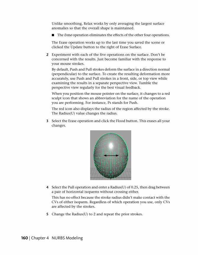
Unlike smoothing, Relax works by only averaging the largest surfaceanomalies so that the overall shape is maintained.
■ The Erase operation eliminates the effects of the other four operations.
The Erase operation works up to the last time you saved the scene orclicked the Update button to the right of Erase Surface.
2 Experiment with each of the five operations on the surface. Don’t beconcerned with the results. Just become familiar with the response toyour mouse strokes.
By default, Push and Pull strokes deform the surface in a direction normal(perpendicular) to the surface. To create the resulting deformation moreaccurately, use Push and Pull strokes in a front, side, or top view whileexamining the results in a separate perspective view. Tumble theperspective view regularly for the best visual feedback.
When you position the mouse pointer on the surface, it changes to a redsculpt icon that shows an abbreviation for the name of the operationyou are performing. For instance, Ps stands for Push.
The red icon also displays the radius of the region affected by the stroke.The Radius(U) value changes the radius.
3 Select the Erase operation and click the Flood button. This erases all yourchanges.
4 Select the Pull operation and enter a Radius(U) of 0.25, then drag betweena pair of horizontal isoparms without crossing either.
This has no effect because the stroke radius didn’t make contact with theCVs of either isoparm. Regardless of which operation you use, only CVsare affected by the strokes.
5 Change the Radius(U) to 2 and repeat the prior strokes.
160 | Chapter 4 NURBS Modeling
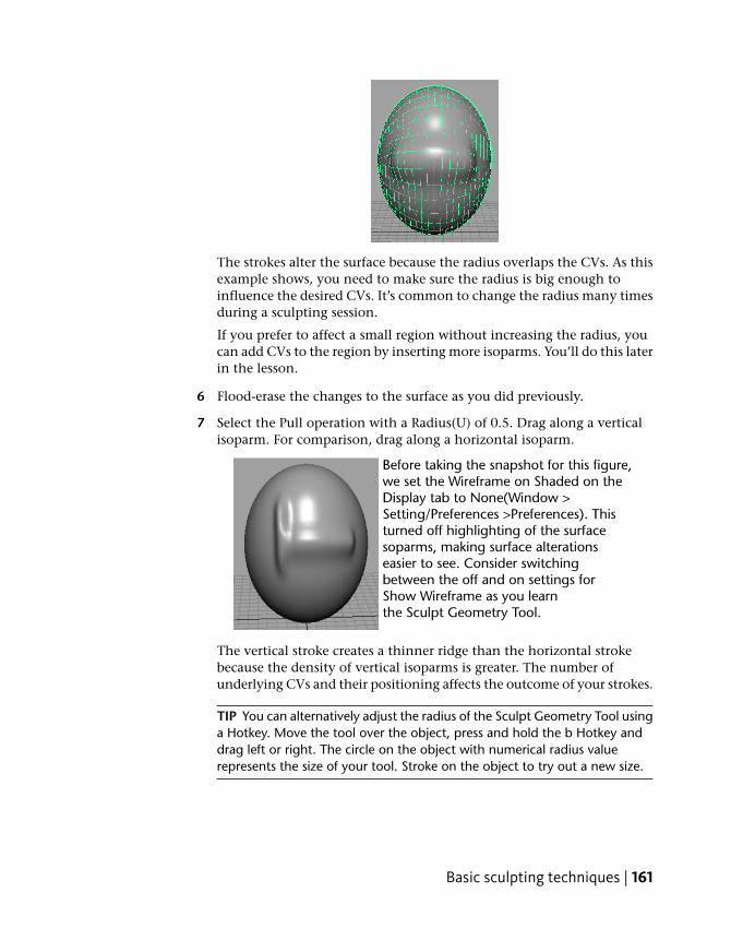
The strokes alter the surface because the radius overlaps the CVs. As thisexample shows, you need to make sure the radius is big enough toinfluence the desired CVs. It’s common to change the radius many timesduring a sculpting session.
If you prefer to affect a small region without increasing the radius, youcan add CVs to the region by inserting more isoparms. You’ll do this laterin the lesson.
6 Flood-erase the changes to the surface as you did previously.
7 Select the Pull operation with a Radius(U) of 0.5. Drag along a verticalisoparm. For comparison, drag along a horizontal isoparm.
The vertical stroke creates a thinner ridge than the horizontal strokebecause the density of vertical isoparms is greater. The number ofunderlying CVs and their positioning affects the outcome of your strokes.
TIP You can alternatively adjust the radius of the Sculpt Geometry Tool usinga Hotkey. Move the tool over the object, press and hold the b Hotkey anddrag left or right. The circle on the object with numerical radius valuerepresents the size of your tool. Stroke on the object to try out a new size.
Basic sculpting techniques | 161
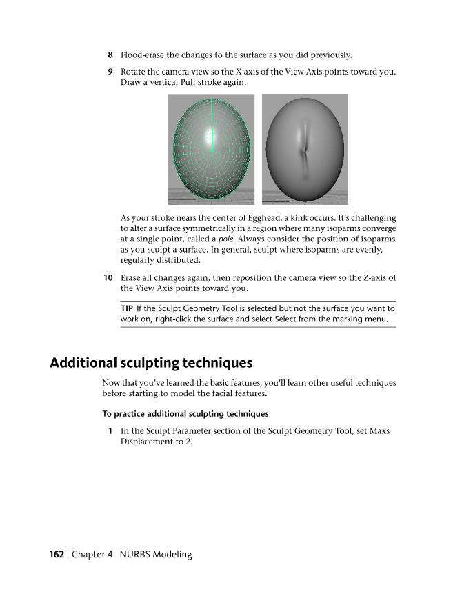
8 Flood-erase the changes to the surface as you did previously.
9 Rotate the camera view so the X axis of the View Axis points toward you.Draw a vertical Pull stroke again.
As your stroke nears the center of Egghead, a kink occurs. It’s challengingto alter a surface symmetrically in a region where many isoparms convergeat a single point, called a pole. Always consider the position of isoparmsas you sculpt a surface. In general, sculpt where isoparms are evenly,regularly distributed.
10 Erase all changes again, then reposition the camera view so the Z-axis ofthe View Axis points toward you.
TIP If the Sculpt Geometry Tool is selected but not the surface you want towork on, right-click the surface and select Select from the marking menu.
Additional sculpting techniquesNow that you’ve learned the basic features, you’ll learn other useful techniquesbefore starting to model the facial features.
To practice additional sculpting techniques
1 In the Sculpt Parameter section of the Sculpt Geometry Tool, set MaxsDisplacement to 2.
162 | Chapter 4 NURBS Modeling
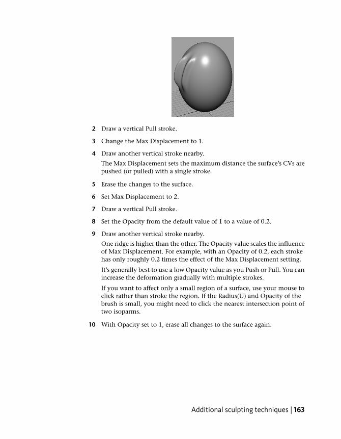
2 Draw a vertical Pull stroke.
3 Change the Max Displacement to 1.
4 Draw another vertical stroke nearby.
The Max Displacement sets the maximum distance the surface’s CVs arepushed (or pulled) with a single stroke.
5 Erase the changes to the surface.
6 Set Max Displacement to 2.
7 Draw a vertical Pull stroke.
8 Set the Opacity from the default value of 1 to a value of 0.2.
9 Draw another vertical stroke nearby.
One ridge is higher than the other. The Opacity value scales the influenceof Max Displacement. For example, with an Opacity of 0.2, each strokehas only roughly 0.2 times the effect of the Max Displacement setting.
It’s generally best to use a low Opacity value as you Push or Pull. You canincrease the deformation gradually with multiple strokes.
If you want to affect only a small region of a surface, use your mouse toclick rather than stroke the region. If the Radius(U) and Opacity of thebrush is small, you might need to click the nearest intersection point oftwo isoparms.
10 With Opacity set to 1, erase all changes to the surface again.
Additional sculpting techniques | 163
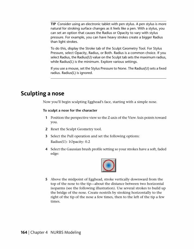
TIP Consider using an electronic tablet with pen stylus. A pen stylus is morenatural for stroking surface changes as it feels like a pen. With a stylus, youcan set an option that causes the Radius or Opacity to vary with styluspressure. For example, you can have heavy strokes create a bigger Radiusthan light strokes.
To do this, display the Stroke tab of the Sculpt Geometry Tool. For StylusPressure, select Opacity, Radius, or Both. Radius is a common choice. If youselect Radius, the Radius(U) value on the Sculpt tab sets the maximum radius,while Radius(L) is the minimum. Explore various settings.
If you use a mouse, set the Stylus Pressure to None. The Radius(U) sets a fixedradius. Radius(L) is ignored.
Sculpting a noseNow you’ll begin sculpting Egghead’s face, starting with a simple nose.
To sculpt a nose for the character
1 Position the perspective view so the Z-axis of the View Axis points towardyou.
2 Reset the Sculpt Geometry tool.
3 Select the Pull operation and set the following options:
Radius(U): 1Opacity: 0.2
4 Select the Gaussian brush profile setting so your strokes have a soft, fadededge:
5 Above the midpoint of Egghead, stroke vertically downward from thetop of the nose to the tip—about the distance between two horizontalisoparms (see the following illustration). Use several strokes to build upthe bridge of the nose. Create nostrils by stroking horizontally to theright of the tip of the nose a few times, then to the left of the tip a fewtimes.
164 | Chapter 4 NURBS Modeling
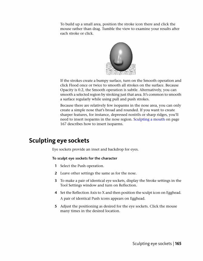
To build up a small area, position the stroke icon there and click themouse rather than drag. Tumble the view to examine your results aftereach stroke or click.
If the strokes create a bumpy surface, turn on the Smooth operation andclick Flood once or twice to smooth all strokes on the surface. BecauseOpacity is 0.2, the Smooth operation is subtle. Alternatively, you cansmooth a selected region by stroking just that area. It’s common to smootha surface regularly while using pull and push strokes.
Because there are relatively few isoparms in the nose area, you can onlycreate a simple nose that’s broad and rounded. If you want to createsharper features, for instance, depressed nostrils or sharp ridges, you’llneed to insert isoparms in the nose region. Sculpting a mouth on page167 describes how to insert isoparms.
Sculpting eye socketsEye sockets provide an inset and backdrop for eyes.
To sculpt eye sockets for the character
1 Select the Push operation.
2 Leave other settings the same as for the nose.
3 To make a pair of identical eye sockets, display the Stroke settings in theTool Settings window and turn on Reflection.
4 Set the Reflection Axis to X and then position the sculpt icon on Egghead.
A pair of identical Push icons appears on Egghead.
5 Adjust the positioning as desired for the eye sockets. Click the mousemany times in the desired location.
Sculpting eye sockets | 165

NOTE If the Reflection setting does not push or pull in the same directionon either side of a NURBS surface you can adjust the Reference Vector to alterthe direction of these operations. In the Sculpt Parameters section select UVVector and turn on Enable UV Vector Adjustment. Click and drag the mouseleft or right to adjust the direction of the U and V reference vectors.
Sculpting eyebrowsEyebrows help define how stern or pleasant a face appears.
To sculpt eyebrows for the character
1 Select the Pull operation. Use the same option settings as for the eyesockets, including Reflection.
2 Position the sculpt icons above the eyes and draw horizontal strokes. Ifnecessary, click positions where you need to build up the eyebrows.Smooth the eyebrows as necessary.
166 | Chapter 4 NURBS Modeling

Sculpting a mouthWith the 30 Sections and 30 Spans specified for the original sphere in thislesson, the large space between isoparms in the mouth region makes itimpossible to create a subtle shape for the lips.
To overcome this problem, you must insert isoparms in the mouth regionbefore sculpting.
To insert additional isoparms
1 Right-click Egghead and select Isoparm from the marking menu.
2 From the Toolbox, choose the Select Tool.
3 Click the horizontal isoparm below the nose and shift-click the next twobelow it so they become yellow.
Sculpting a mouth | 167

4 Select Edit NURBS > Insert Isoparms > . In the options window, turnon Between Selections, enter a value of 2 for # Isoparms to Insert, thenclick Insert.
This inserts two extra isoparms between each pair of selected isoparms,for a total of four extra isoparms. This provides enough CVs to createsubtlety in the mouth.
You might want to add vertical isoparms at the lips in a similar way. Theextra isoparms would also be useful if you were to later enhance the shapeof the nose. Insert isoparms only where needed. More isoparms meansslower processing speed.
In any case, do not change the number of isoparms by editing the originalnumber of Sections and Spans in the makeNurbSphere history node. Thiswill reshape your sculpted surface undesirably.
To sculpt a mouth for the character
1 Select the Sculpt Geometry Tool again.
2 Select the Push operation. Enter 0.2 for Radius(U). In the Stroke tab, makesure Reflection is turned on.
3 Starting at the center of the area appropriate for the indentation betweenthe lips, stroke outward from the center. It’s best to start the stroke withthe dual icons on top of one another (in other words, only one icon isdisplayed).
4 Select the Pull operation and set the Radius(U) to 0.3. Using a similartechnique as for the prior step, stroke the upper lip. Repeat for the lowerlip.
168 | Chapter 4 NURBS Modeling

NOTE It might be easier to push or pull the lips with the Ref. Vector set toZ Axis. This moves the region you stroke in the world Z-Axis direction. Thedefault Normal setting moves the region in a direction normal (perpendicular)to the surface. Because the normal direction on a lip might be up, down, orstraight out, depending on the part of the lip you stroke, there’s morepossibility of undesired results when you use the Normal setting.
Sculpting other facial featuresYou can now optionally add other facial features. Consider these tips:
■ For facial features such as the chin, cheeks, and forehead, use a Radius(U)larger than 1 and start with a Maximum Displacement between 0.5 and1.
■ Insert isoparms wherever you want to add extra detail with the SculptGeometry Tool.
■ To create eyeballs for the sockets, create a sphere and scale it as necessaryto fit the socket. You might want to increase the eyeball’s Scale X value tomake it oblong. To duplicate the eyeball, and make a mirrored copy of theoriginal you’ll first need to set the pivot point for the eyeball to be at theorigin 0, 0, 0 using the following steps. With the sphere selected, press theInsert (Windows and Linux) or Home (Mac OS X) key so that the sphere’spivot point is displayed. Next move the pivot point to the origin using theX hotkey so that the pivot snaps to the grid at 0, 0, 0. Select Insert (Home)to turn off the pivot point display. Finally, use Edit > Duplicate Special >
and set the Scale setting to -1, 1, 1. This makes the new eyeball amirrored duplicate of the original on the opposite side of Egghead’s face.Position the eyeballs in the sockets. Parent the eyeballs to Egghead.
Sculpting other facial features | 169
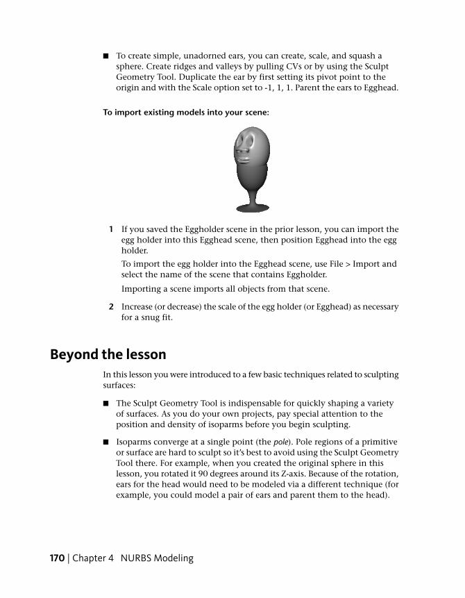
■ To create simple, unadorned ears, you can create, scale, and squash asphere. Create ridges and valleys by pulling CVs or by using the SculptGeometry Tool. Duplicate the ear by first setting its pivot point to theorigin and with the Scale option set to -1, 1, 1. Parent the ears to Egghead.
To import existing models into your scene:
1 If you saved the Eggholder scene in the prior lesson, you can import theegg holder into this Egghead scene, then position Egghead into the eggholder.
To import the egg holder into the Egghead scene, use File > Import andselect the name of the scene that contains Eggholder.
Importing a scene imports all objects from that scene.
2 Increase (or decrease) the scale of the egg holder (or Egghead) as necessaryfor a snug fit.
Beyond the lessonIn this lesson you were introduced to a few basic techniques related to sculptingsurfaces:
■ The Sculpt Geometry Tool is indispensable for quickly shaping a varietyof surfaces. As you do your own projects, pay special attention to theposition and density of isoparms before you begin sculpting.
■ Isoparms converge at a single point (the pole). Pole regions of a primitiveor surface are hard to sculpt so it’s best to avoid using the Sculpt GeometryTool there. For example, when you created the original sphere in thislesson, you rotated it 90 degrees around its Z-axis. Because of the rotation,ears for the head would need to be modeled via a different technique (forexample, you could model a pair of ears and parent them to the head).
170 | Chapter 4 NURBS Modeling
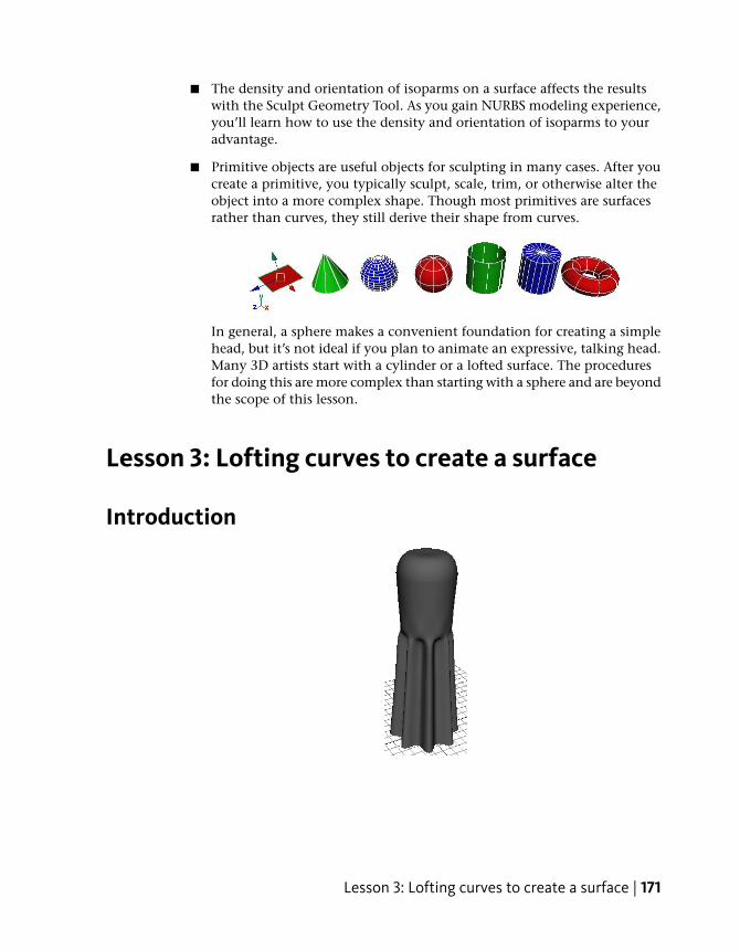
■ The density and orientation of isoparms on a surface affects the resultswith the Sculpt Geometry Tool. As you gain NURBS modeling experience,you’ll learn how to use the density and orientation of isoparms to youradvantage.
■ Primitive objects are useful objects for sculpting in many cases. After youcreate a primitive, you typically sculpt, scale, trim, or otherwise alter theobject into a more complex shape. Though most primitives are surfacesrather than curves, they still derive their shape from curves.
In general, a sphere makes a convenient foundation for creating a simplehead, but it’s not ideal if you plan to animate an expressive, talking head.Many 3D artists start with a cylinder or a lofted surface. The proceduresfor doing this are more complex than starting with a sphere and are beyondthe scope of this lesson.
Lesson 3: Lofting curves to create a surface
Introduction
Lesson 3: Lofting curves to create a surface | 171

Another method for creating NURBS surfaces is to loft a series of curves thatdefine the cross section of your desired surface form. Lofting a surface workslike stretching a skin over each of the cross sections to create the final surface.
In this lesson, you learn additional NURBS surfacing techniques by using theLoft tool to create the body of a salt shaker. You will also create the cap forthe salt shaker by modifying the shape of a primitive sphere.
In this lesson you learn how to:
■ Modify the outline of a circle primitive by editing the position of its CVs.
■ Use the magnet snap feature.
■ Loft cross section curves to create a NURBS surface using the Loft tool.
■ Edit the form of an existing primitive object by moving its CVs.
■ Parent one object to another using the Outliner.
Creating profile curves for a surfaceYou begin the lesson by creating a pair of profile curves. You then createseveral copies of these curves to form the skeletal contours of the salt shaker’ssurface.
To create profile curves for the salt shaker’s body
1 Make sure you’ve done the steps in Preparing for the lessons on page 149.
2 Select Create > NURBS Primitives > Circle > . In the options window,select Edit > Reset Settings, enter the following values, then click theApply button:
■ Radius: 4
■ Number of Sections: 24
The Radius sets the size of the circle in grid units. A value of 4 creates acircle with enough size so that you can use the grid for convenient sizecomparison.
The Number of Sections sets the number of CVs in the circle. By using24 CVs, you can create a circle with the subtle contours required in thislesson. Display the CVs of the circle to see the 24 CVs.
172 | Chapter 4 NURBS Modeling
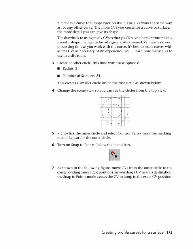
A circle is a curve that loops back on itself. The CVs work the same wayas for any other curve. The more CVs you create for a curve or surface,the more detail you can give its shape.
The drawback to using many CVs is that you’ll have a harder time makingsmooth shape changes to broad regions. Also, more CVs means slowerprocessing time as you work with the curve. It’s best to make curves withas few CVs as necessary. With experience, you’ll learn how many CVs touse in a situation.
3 Create another circle, this time with these options:
■ Radius: 2
■ Number of Sections: 24
This creates a smaller circle inside the first circle as shown below.
4 Change the scene view so you can see the circles from the top view.
5 Right-click the inner circle and select Control Vertex from the markingmenu. Repeat for the outer circle.
6 Turn on Snap to Points (below the menu bar).
7 As shown in the following figure, move CVs from the outer circle to thecorresponding inner circle positions. As you drag a CV near its destination,the Snap to Points mode causes the CV to jump to the exact CV position.
Creating profile curves for a surface | 173

8 Turn off Snap to Points. Turn off the display of CVs for both circles byright-clicking on the circles and selecting Object Mode from the markingmenu.
Duplicating curvesIn the next steps, you’ll create several copies of the previously created circles(also called curves) to form the skeletal contours of the salt shaker’s surface.
To duplicate curves for the lofted surface
1 Right-click the outer curve and choose Select from the marking menu.
2 Select Edit > Duplicate Special > . In the options window, select Edit> Reset Settings, enter the following values, then click Duplicate Special:
■ Translate: 0 3 0
■ Scale: 0.93 1 0.93
■ Number of Copies: 4
174 | Chapter 4 NURBS Modeling

This creates four copies of the original curve, each translated three unitsabove the last, and each scaled smaller than the last.
3 Select the inner circle and then move it to 0, 13, 0 by entering thesetranslate values in the Channel Box. Increase its Scale attributes to 1.33,1.33, 1.33..
4 Use Edit > Duplicate Special > with the following options:
■ Translate: 0 2 0
■ Scale: 1.05 1 1.05
■ Number of Copies: 3
This creates three copies of the circle, each translated two units abovethe last, and each bigger than the last.
Lofting a surfaceYou’ve created a total of nine curves. In the next steps, you loft these curvesinto a surface that matches the contours of their perimeters. Above themidpoint of the surface, the shape will change from a flower-shaped perimeterto a circular perimeter.
To loft a surface for the salt shaker’s body
1 Starting from the bottom circle, and working towards the top, shift-selectall the circles, one at a time.
The order of selection is important when shift-selecting for a loftoperation. You must start with the bottom flower-shaped circle and endwith the top circular-shaped circle. Alternatively, you can drag a selectionbox around the circles. The surface to be lofted will be based on theselection order of the curves.
Lofting a surface | 175
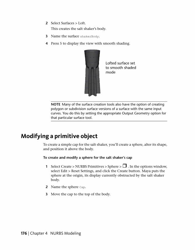
2 Select Surfaces > Loft.
This creates the salt shaker’s body.
3 Name the surface shakerBody.
4 Press 5 to display the view with smooth shading.
NOTE Many of the surface creation tools also have the option of creatingpolygon or subdivision surface versions of a surface with the same inputcurves. You do this by setting the appropriate Output Geometry option forthat particular surface tool.
Modifying a primitive objectTo create a simple cap for the salt shaker, you’ll create a sphere, alter its shape,and position it above the body.
To create and modify a sphere for the salt shaker’s cap
1 Select Create > NURBS Primitives > Sphere > . In the options window,select Edit > Reset Settings, and click the Create button. Maya puts thesphere at the origin, its display currently obstructed by the salt shakerbody.
2 Name the sphere Cap.
3 Move the cap to the top of the body.
176 | Chapter 4 NURBS Modeling
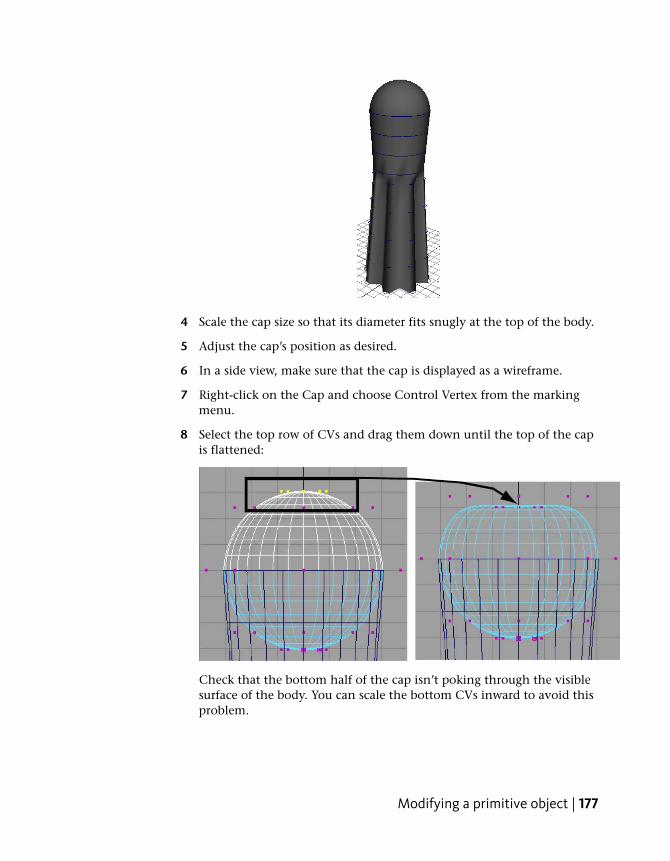
4 Scale the cap size so that its diameter fits snugly at the top of the body.
5 Adjust the cap’s position as desired.
6 In a side view, make sure that the cap is displayed as a wireframe.
7 Right-click on the Cap and choose Control Vertex from the markingmenu.
8 Select the top row of CVs and drag them down until the top of the capis flattened:
Check that the bottom half of the cap isn’t poking through the visiblesurface of the body. You can scale the bottom CVs inward to avoid thisproblem.
Modifying a primitive object | 177

Using the Outliner to parent objectsThe Outliner is an editor that is useful for quickly examining the structureand components of a scene. You can use the Outliner to quickly parent objectsto create an object hierarchy.
To parent an object using the Outliner
1 From the main menu, select In the main menu bar:.
The Outliner window is displayed. A list of the scene’s components islisted in the Outliner.
2 In the Outliner, click on the word Cap to select it.
3 Parent the cap to the body by middle-mouse dragging Cap ontoshakerBody1 in the Outliner.
178 | Chapter 4 NURBS Modeling

By parenting the objects, you can move, rotate, or scale the cap and thebody as a single entity by selecting only the body.
Notice that the salt shaker displays horizontal curves that wrap aroundthe body. The curves are the original circles you used to loft the surface.Because these curves are part of the surface’s construction history, youcan alter their shape if you decide you want to alter the shape of the bodyand the body will update based on the construction history.
If you prefer not to see the curves in the scene view, select the curves andselect Hide Selection. The curves won’t appear when you render an imageof the scene. Maya displays only surfaces, not curves, in rendered images.
Beyond the lessonIn this lesson you were introduced to the basic techniques related to loftingcurves to create NURBS surfaces:
■ You made a salt shaker with two surfaces: a body made from lofted curvesand a cap made from an altered sphere. An advantage of creating a separatesurface for the cap and base is that you can easily give each a differentcolor or texture, for example, one chrome and the other marble. Anotheradvantage of creating a separate cap is that you can animate the objectseparately. For example, you could choose to animate the cap unscrewingfrom the shakerBody.
■ You used a Loft operation rather than a Revolve operation to create thebody. The vertical corrugations on the surface would be impossible tocreate by revolving a curve.
■ You can alter the position of the profile curves and the shape of the shakerwill update because of the construction history. If you’re certain you won’tchange the body’s shape by editing the shape of the lofted curves, you candelete the body’s construction history to quicken Maya’s processing ofyour interaction with the surface. (For a surface as simple as the salt shaker,deleting the history won’t boost processing much.)
■ There are many other useful tools for creating and editing surfaces. For aglimpse of the possibilities, take a look at the Surfaces menu and the EditNURBS menu.
If you want to learn more about a particular tool or feature that has beenpresented in this lesson, please refer to the Maya Help.
Beyond the lesson | 179

180
Subdivision Surfaces
IntroductionSubdivision surfaces are a hybrid surface type that possess characteristics of bothNURBS and polygonal surfaces as well as other features not offered by the othersurface types. Like NURBS, subdivision surfaces are capable of producing smoothorganic forms and can be shaped using relatively few control vertices. Likepolygonal surfaces, subdivision surfaces let you extrude specific areas and createadditional detail in your surfaces. You do this by working at different levels ofdetail on the subdivision surface and switching between the levels whennecessary. With a subdivision surface you can build a smooth organic objectfrom a single primitive and not be concerned about attaching or stitching thevarious surfaces together as you would for a NURBS surface.
Preparing for the lessonTo ensure the lesson works as described, do these steps before beginning:
1 Review the Polygon Modeling lesson in this guide. Knowledge of polygonalmodeling tools is essential to becoming proficient in subdivision surfacemodeling.
2 If you have not already done so, copy the GettingStarted folder from itsinstallation location to your projects directory. Then, set theGettingStarted directory as your Maya project. For more information, seeCopying and setting the Maya project on page 25.
3 Create a new scene.
4 Select the Surfaces menu set.
5
181
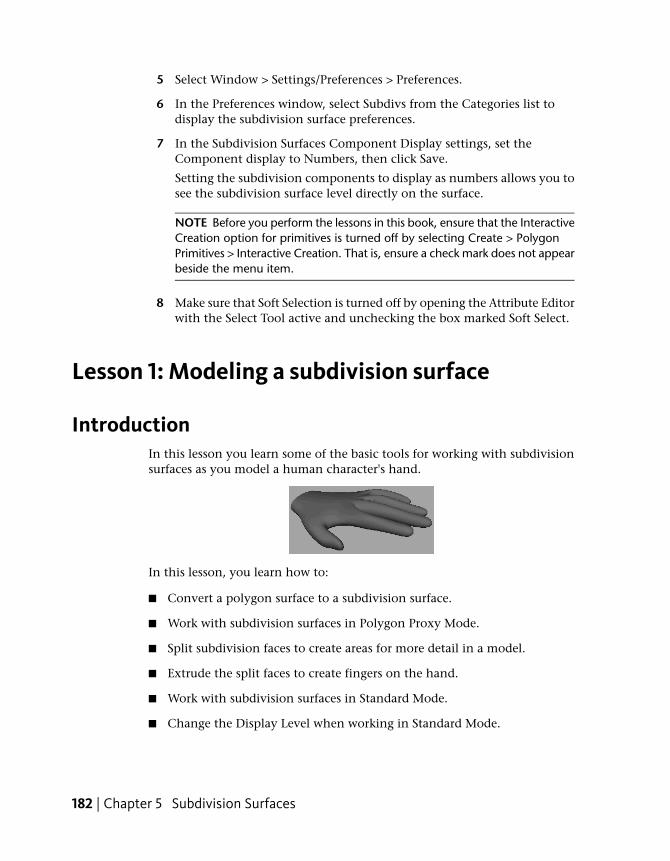
5 Select Window > Settings/Preferences > Preferences.
6 In the Preferences window, select Subdivs from the Categories list todisplay the subdivision surface preferences.
7 In the Subdivision Surfaces Component Display settings, set theComponent display to Numbers, then click Save.
Setting the subdivision components to display as numbers allows you tosee the subdivision surface level directly on the surface.
NOTE Before you perform the lessons in this book, ensure that the InteractiveCreation option for primitives is turned off by selecting Create > PolygonPrimitives > Interactive Creation. That is, ensure a check mark does not appearbeside the menu item.
8 Make sure that Soft Selection is turned off by opening the Attribute Editorwith the Select Tool active and unchecking the box marked Soft Select.
Lesson 1: Modeling a subdivision surface
IntroductionIn this lesson you learn some of the basic tools for working with subdivisionsurfaces as you model a human character's hand.
In this lesson, you learn how to:
■ Convert a polygon surface to a subdivision surface.
■ Work with subdivision surfaces in Polygon Proxy Mode.
■ Split subdivision faces to create areas for more detail in a model.
■ Extrude the split faces to create fingers on the hand.
■ Work with subdivision surfaces in Standard Mode.
■ Change the Display Level when working in Standard Mode.
182 | Chapter 5 Subdivision Surfaces

■ Add more detail to subdivision surface models using Refine SelectedComponents.
■ Create a crease along a vertex edge.
Creating a subdivision surfaceYou begin the lesson by creating a polygonal cube. You’ll convert this cubeto a subdivision surface that will be the foundation of the hand. The reasonfor starting with a polygonal surface and converting it to a subdivision surfaceis that you can thereafter edit the object’s shape with more versatility: youcan edit with subdivision surface tools and polygonal tools.
To create a polygon cube
➤ Select Create > Polygon Primitives > Cube > . In the options window,select Edit > Reset Settings. Then enter the following values and click theCreate button.
■ Width: 8
■ Height: 2.5
■ Depth: 8
The resulting polygonal cube is roughly proportional to the palm of ahand.
To convert a polygonal cube to a subdivision surface
1 To convert the polygonal cube to a subdivision surface, select Modify >Convert > NURBS to Subdiv, Polygons to Subdiv.
Creating a subdivision surface | 183

2 Press 3 on your keyboard (to select Display > Subdiv Surfaces > Fine).
3 Press 5 (to select Shading > Smooth Shade All).
With the smoothness set to Fine, you can see that the conversion to asubdivision surface creates a rounded, smooth shape. By pressing 3, thesubdivision surface is displayed more precisely in the scene view. Thisgives a closer approximation of what the surface will look like when youcreate a rendered image of the scene.
As an alternative, you could have chosen a Rough smoothness (press 1)so that Maya processes your editing changes in the scene view morequickly. Regardless of the smoothness in the scene view, surfaces alwaysare displayed precisely in rendered images of the scene.
To display a subdivision surface in polygon proxy mode
➤ Select Subdiv Surfaces > Polygon Proxy Mode.
184 | Chapter 5 Subdivision Surfaces
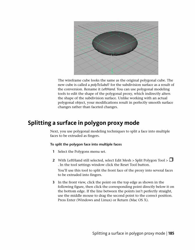
The wireframe cube looks the same as the original polygonal cube. Thenew cube is called a polyToSubd1 for the subdivision surface as a result ofthe conversion. Rename it LeftHand. You can use polygonal modelingtools to edit the shape of the polygonal proxy, which indirectly altersthe shape of the subdivision surface. Unlike working with an actualpolygonal object, your modifications result in perfectly smooth surfacechanges rather than faceted changes.
Splitting a surface in polygon proxy modeNext, you use polygonal modeling techniques to split a face into multiplefaces to be extruded as fingers.
To split the polygon face into multiple faces
1 Select the Polygons menu set.
2 With LeftHand still selected, select Edit Mesh > Split Polygon Tool >. In the tool settings window click the Reset Tool button.
You’ll use this tool to split the front face of the proxy into several facesto be extruded into fingers.
3 In the front view, click the point on the top edge as shown in thefollowing figure, then click the corresponding point directly below it onthe bottom edge. If the line between the points isn’t perfectly straight,use the middle mouse to drag the second point to the correct position.Press Enter (Windows and Linux) or Return (Mac OS X).
Splitting a surface in polygon proxy mode | 185

This splits the face into two faces. You’ll extrude the left face into a fingerlater.
4 Repeat the preceding two steps as necessary to split the face as follows:
Notice how splitting the face into multiple faces alters the shape of thesubdivision surface. The front part of the subdivision surface nowresembles the proxy shape more. If you were to split the front face severalmore times, especially near the outer edges, the subdivision surface wouldsharpen and resemble the proxy shape even more. More faces means finercontrol, often at the expense of making the surface harder to work with.
With the added faces, the subdivision surface looks a bit like the palm ofa hand. You’ll build upon this shape to create a left hand with palm facingdownward and fingers extruded outward. You’ll extrude the wide facesinto fingers, and you’ll leave the narrow faces as webbing between thefingers.
186 | Chapter 5 Subdivision Surfaces
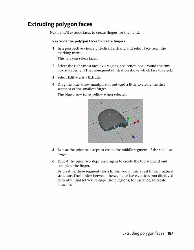
Extruding polygon facesNext, you’ll extrude faces to create fingers for the hand.
To extrude the polygon faces to create fingers
1 In a perspective view, right-click LeftHand and select Face from themarking menu.
This lets you select faces.
2 Select the right-most face by dragging a selection box around the tinybox at its center. (The subsequent illustration shows which face to select.)
3 Select Edit Mesh > Extrude.
4 Drag the blue arrow manipulator outward a little to create the firstsegment of the smallest finger.
The blue arrow turns yellow when selected.
5 Repeat the prior two steps to create the middle segment of the smallestfinger.
6 Repeat the prior two steps once again to create the top segment andcomplete the finger.
By creating three segments for a finger, you mimic a real finger’s naturalstructure. The borders between the segments have vertices (not displayedcurrently) that let you reshape those regions, for instance, to createknuckles.
Extruding polygon faces | 187
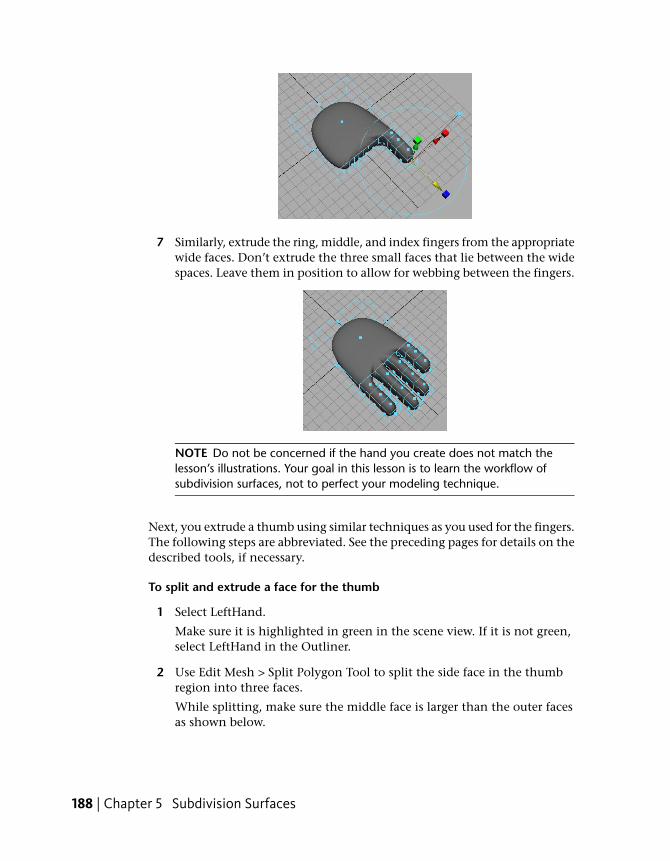
7 Similarly, extrude the ring, middle, and index fingers from the appropriatewide faces. Don’t extrude the three small faces that lie between the widespaces. Leave them in position to allow for webbing between the fingers.
NOTE Do not be concerned if the hand you create does not match thelesson’s illustrations. Your goal in this lesson is to learn the workflow ofsubdivision surfaces, not to perfect your modeling technique.
Next, you extrude a thumb using similar techniques as you used for the fingers.The following steps are abbreviated. See the preceding pages for details on thedescribed tools, if necessary.
To split and extrude a face for the thumb
1 Select LeftHand.
Make sure it is highlighted in green in the scene view. If it is not green,select LeftHand in the Outliner.
2 Use Edit Mesh > Split Polygon Tool to split the side face in the thumbregion into three faces.
While splitting, make sure the middle face is larger than the outer facesas shown below.
188 | Chapter 5 Subdivision Surfaces

3 Extrude the middle face and drag it directly outward.
4 Click the surrounding blue circle and use the rotate manipulator to aimit in a direction appropriate for a thumb.
5 Extrude three times more to create each segment of the thumb. Use theextrusion manipulator to rotate, move, and scale each extrusion to createthe desired shape of a thumb. Use the following figure as a guideline.Again, it’s unnecessary to match the illustration or create a realistic thumbfor this lesson.
The extrusion manipulator is easy to figure out by clicking and draggingits various elements. If necessary, you can also use the conventional Move,Scale, and Rotate Tools to reshape the faces that control the thumb’sshape.
6 fIn the scene view, right-click LeftHand and select Vertex from themarking menu. The purple vertices at the corners of the faces control theadjacent region of the hand.
Extruding polygon faces | 189

7 Make coarse adjustments to various parts of the hand by repositioningthe vertices with the Move, Scale, and Rotate Tools.
The Move Tool works on individual vertices or groups of vertices. Rotateand Scale works on two or more vertices. Undo any changes you don’tlike using Ctrl-Z (Windows and Linux) or Control-z (Mac OS X).
Try to create the approximate thickness, length, and curvature of a cartooncharacter’s hand and fingers. There’s no need for perfection. You’ll refinethe fingers later.
Deleting polygon facesIn the next steps, you delete a face in order to create a hole in the wrist whereyou might choose to attach an arm. Though you won’t create and attach anarm in this lesson, it’s useful to learn the technique for future use.
To create a hole at the wrist by deleting a face
1 In the scene view, right-click LeftHand and select Face from the markingmenu.
2 Select the face at the wrist and press Delete to create a hole where youcould attach an arm.
190 | Chapter 5 Subdivision Surfaces

3 Scale the four vertices that surround the hole and scale them inward tonarrow the wrist region of the hand.
Subdivision surface levelsNext, you refine the shape of the fingers by working in Standard Mode. InStandard Mode, you can make edits to mesh vertices, edges, or faces at differentlevels of refinement, that are not possible in Polygon Proxy mode. The differentlevels of refinement are referred to as subdivision surface levels.
To refine the fingers using subdivision surface levels
1 Select LeftHand.
2 Select the Surfaces menu set.
3 Select Subdiv Surfaces > Standard Mode. This switches to a mode thatlets you modify the surface at various levels of detail to suit your needs.
4 In the scene view, right-click LeftHand and select Vertex from the markingmenu.
Subdivision surface levels | 191

This displays 0s on the surface in the same positions as the vertices inPolygon Proxy mode. In fact, the 0s are vertices.
The number 0 refers to the level of detail you are capable of editing. The0 level is identical to the coarse control possible in Polygon Proxy modeby manipulating the vertices. You can move, rotate, and scale the 0s toalter the shape of the surface just as you did for vertices in Polygon Proxymode.
5 Right-click the surface and select Display Level > 1.
Though the 1s are displayed in the same regions as the 0s were previously,there are many more 1s displayed. The 1s are also vertices, and theirincreased presence means you can refine the shape with more subtlety.
6 Refine the shape of the fingers, thumb, and hand as desired by selectingvarious level 1 vertices and moving, scaling, and rotating them with thetransformation tools. (Scaling and rotating has effect only if you selecttwo or more vertices.)
It’s essential to tumble the camera from various perspectives to make sureyou’ve selected only the desired vertices.
To return to level 0 to alter the shape with fewer vertices, right-click thesurface and select Display Level > 0. Each level has advantages. Level 1allows finer control because there are more vertices. Level 0 allows controlof broader regions, and it’s often easier to select the desired vertices since
192 | Chapter 5 Subdivision Surfaces
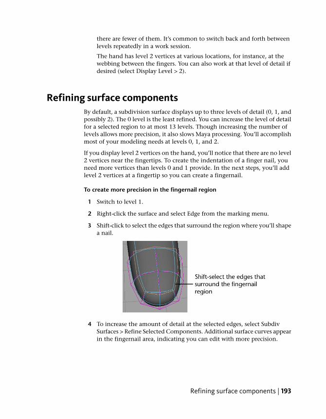
there are fewer of them. It’s common to switch back and forth betweenlevels repeatedly in a work session.
The hand has level 2 vertices at various locations, for instance, at thewebbing between the fingers. You can also work at that level of detail ifdesired (select Display Level > 2).
Refining surface componentsBy default, a subdivision surface displays up to three levels of detail (0, 1, andpossibly 2). The 0 level is the least refined. You can increase the level of detailfor a selected region to at most 13 levels. Though increasing the number oflevels allows more precision, it also slows Maya processing. You’ll accomplishmost of your modeling needs at levels 0, 1, and 2.
If you display level 2 vertices on the hand, you’ll notice that there are no level2 vertices near the fingertips. To create the indentation of a finger nail, youneed more vertices than levels 0 and 1 provide. In the next steps, you’ll addlevel 2 vertices at a fingertip so you can create a fingernail.
To create more precision in the fingernail region
1 Switch to level 1.
2 Right-click the surface and select Edge from the marking menu.
3 Shift-click to select the edges that surround the region where you’ll shapea nail.
4 To increase the amount of detail at the selected edges, select SubdivSurfaces > Refine Selected Components. Additional surface curves appearin the fingernail area, indicating you can edit with more precision.
Refining surface components | 193

5 In the scene view, right-click LeftHand and select Vertex from the markingmenu. This displays additional level 2 vertices in the fingertip region.
6 Select Modify > Transformation Tools > Move Tool, Rotate Tool, Scale
Tool, Show Manipulator Tool > . In the Tool Settings window, turnon Normal, then close the window. You can thereafter use the Move Toolmanipulator to move vertices in a direction normal (perpendicular) tothe surface.
7 Select the vertices in the nail region.
NOTE Be careful to select only those vertices in the nail region. You mayneed to tumble the camera to ensure that all extra vertices are de-selected.
8 Drag the Move Tool’s N manipulator down slightly to form the depressionof a fingernail bed.
194 | Chapter 5 Subdivision Surfaces

Creating a crease in a subdivision surfaceOne of the unique features of subdivision surfaces is that it’s easy to create acrease or ridge on a smooth surface. You’ll do this in the next steps.
To crease the edge of the fingernail
1 Switch to Edge selection mode and shift-click the edges around the nailto select them. (It might be easier to see the desired edges by first selectingShading > Wireframe.)
2 After you select the edges, select Subdiv Surfaces > Full Crease Edge/Vertex.
Once you crease an edge, it displays with a dashed line as a visualreminder that the edge has been creased. If you change your mind, youcan remove the crease using Subdiv Surfaces > Uncrease Edge/Vertex.
3 To create a ridge at the edge of the nail, switch to Vertex selection modeand select the level 2 vertices on the skin at the perimeter of the previouslyselected edges. Move them up so that the skin’s juncture with the nailforms a slight ridge.
Creating a crease in a subdivision surface | 195
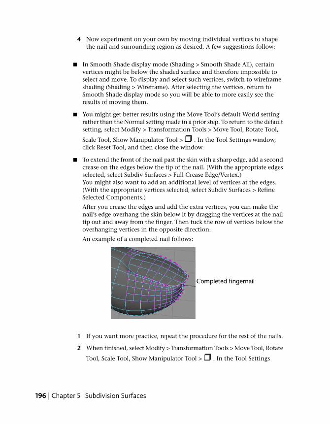
4 Now experiment on your own by moving individual vertices to shapethe nail and surrounding region as desired. A few suggestions follow:
■ In Smooth Shade display mode (Shading > Smooth Shade All), certainvertices might be below the shaded surface and therefore impossible toselect and move. To display and select such vertices, switch to wireframeshading (Shading > Wireframe). After selecting the vertices, return toSmooth Shade display mode so you will be able to more easily see theresults of moving them.
■ You might get better results using the Move Tool’s default World settingrather than the Normal setting made in a prior step. To return to the defaultsetting, select Modify > Transformation Tools > Move Tool, Rotate Tool,
Scale Tool, Show Manipulator Tool > . In the Tool Settings window,click Reset Tool, and then close the window.
■ To extend the front of the nail past the skin with a sharp edge, add a secondcrease on the edges below the tip of the nail. (With the appropriate edgesselected, select Subdiv Surfaces > Full Crease Edge/Vertex.)You might also want to add an additional level of vertices at the edges.(With the appropriate vertices selected, select Subdiv Surfaces > RefineSelected Components.)
After you crease the edges and add the extra vertices, you can make thenail’s edge overhang the skin below it by dragging the vertices at the nailtip out and away from the finger. Then tuck the row of vertices below theoverhanging vertices in the opposite direction.
An example of a completed nail follows:
1 If you want more practice, repeat the procedure for the rest of the nails.
2 When finished, select Modify > Transformation Tools > Move Tool, Rotate
Tool, Scale Tool, Show Manipulator Tool > . In the Tool Settings
196 | Chapter 5 Subdivision Surfaces

window, click Reset Tool, and then close the window. This returns theMove Tool to its default settings. This will avoid confusion in futurelessons.
Beyond the lessonIn this lesson, you were introduced to some basic techniques related tosubdivision surface modeling:
■ Modeling with subdivision surfaces is an easy way to create intricate,smooth objects such as human hands and faces. The ability to createextrusions, subtle surface alterations, and sharp edges means there areinnumerable types of objects you can model.
■ Many of the techniques used in modeling polygonal surfaces are applicableto subdivision surfaces.
There are many other features related to subdivision surfaces not covered inthis lesson. These include the ability to:
■ Convert a NURBS surface to subdivision surface.
■ Convert a subdivision surface to a polygonal or NURBS surface.
■ Create subdivision surface primitive shapes from the Create > SubdivPrimitives menu: Sphere, Cube, Cylinder, Cone, Plane, and Torus. Withthese shapes, you can quickly start your subdivision surface model withoutconverting from polygons or NURBS surfaces.
■ Attach two subdivision surfaces to form a single surface, for instance, tomerge a hand and an arm.
■ Create a mirrored copy of a subdivision surface.
■ You can sculpt subdivision surfaces using the Sculpt Geometry Tool.If you want to learn more about a particular tool or feature that has beenpresented in this lesson, refer to the Maya Help.
Beyond the lesson | 197

198

Animation
IntroductionMaya lets you apply action to the objects in your 3D scene. In Maya, when anobject or attribute changes in relation to time, it is referred to as being animated.
Maya provides a large selection of tools to help you animate the objects in yourscene. You may decide to use a combination of several techniques to achieveyour desired results.
In this chapter, you learn some common techniques and features that highlightMaya’s computer animation technology:
■ Lesson 1 Keyframes and the Graph Editor: Introduction on page 200
■ Lesson 2 Set Driven Key: Introduction on page 215
■ Lesson 3 Path animation: Introduction on page 220
■ Lesson 4 Nonlinear animation with Trax: Introduction on page 239
■ Lesson 5 Inverse kinematics: Introduction on page 276
Preparing for the lessonsTo ensure the lessons work as described, do these steps before beginning:
1 Select Window > Settings/Preferences > Preferences. Click the Settingscategory and set the Time option to Film (24 fps) so your animation playsat the rate of 24 frames per second. Click the Save button.
6
199
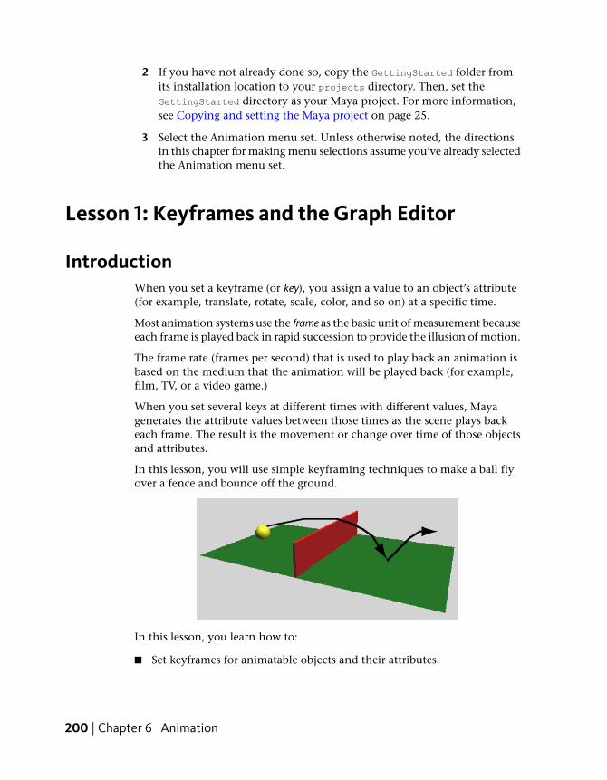
2 If you have not already done so, copy the GettingStarted folder fromits installation location to your projects directory. Then, set theGettingStarted directory as your Maya project. For more information,see Copying and setting the Maya project on page 25.
3 Select the Animation menu set. Unless otherwise noted, the directionsin this chapter for making menu selections assume you’ve already selectedthe Animation menu set.
Lesson 1: Keyframes and the Graph Editor
IntroductionWhen you set a keyframe (or key), you assign a value to an object’s attribute(for example, translate, rotate, scale, color, and so on) at a specific time.
Most animation systems use the frame as the basic unit of measurement becauseeach frame is played back in rapid succession to provide the illusion of motion.
The frame rate (frames per second) that is used to play back an animation isbased on the medium that the animation will be played back (for example,film, TV, or a video game.)
When you set several keys at different times with different values, Mayagenerates the attribute values between those times as the scene plays backeach frame. The result is the movement or change over time of those objectsand attributes.
In this lesson, you will use simple keyframing techniques to make a ball flyover a fence and bounce off the ground.
In this lesson, you learn how to:
■ Set keyframes for animatable objects and their attributes.
200 | Chapter 6 Animation
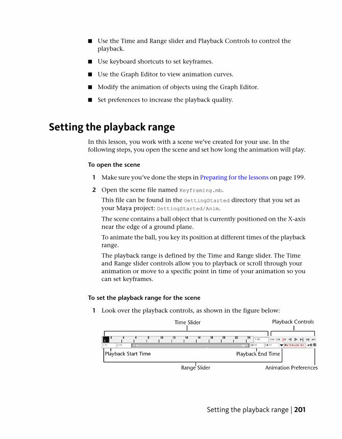
■ Use the Time and Range slider and Playback Controls to control theplayback.
■ Use keyboard shortcuts to set keyframes.
■ Use the Graph Editor to view animation curves.
■ Modify the animation of objects using the Graph Editor.
■ Set preferences to increase the playback quality.
Setting the playback rangeIn this lesson, you work with a scene we’ve created for your use. In thefollowing steps, you open the scene and set how long the animation will play.
To open the scene
1 Make sure you’ve done the steps in Preparing for the lessons on page 199.
2 Open the scene file named Keyframing.mb.
This file can be found in the GettingStarted directory that you set asyour Maya project: GettingStarted/Anim.
The scene contains a ball object that is currently positioned on the X-axisnear the edge of a ground plane.
To animate the ball, you key its position at different times of the playbackrange.
The playback range is defined by the Time and Range slider. The Timeand Range slider controls allow you to playback or scroll through youranimation or move to a specific point in time of your animation so youcan set keyframes.
To set the playback range for the scene
1 Look over the playback controls, as shown in the figure below:
Setting the playback range | 201

The Time Slider displays the playback range and keys you’ve set for aselected object. Keys are displayed as red lines. The box at the right ofthe Time Slider lets you set the current frame (time) of the animation.
The Playback Controls control animation playback. You may recognizethe conventional buttons for play and rewind (return to the start time).The stop button appears only when the animation is playing. To findout which operation a button represents, hold the mouse pointer overit.
The Animation Preferences button displays a window for settinganimation preference settings such as the playback speed.
The Range Slider controls the range of frames that play when you clickthe play button.
The above items will have more relevance as you work through this lesson.After you complete this lesson, experiment with these items to learn morewhat they do.
The playback range is currently set at a range of 1 to 24. At a defaultplayback rate of 24 frames per second, the scene can play for one second.Because you’ll animate the ball for a few more seconds than this, youneed to lengthen the playback range.
2 In the Playback End Time box (see above), enter 72.
A frame rate of 24 frames per second (fps) is the frame rate used for motionpicture film. For video, the frame rate can be 30 fps (NTSC) or 25 fps(PAL) depending on the format being used.
With a playback range of 1 to 72, you’ll be able to create three secondsof animation. (72 frames divided by 24 frames per second = 3 seconds.)This is enough time for the short animation you’ll create in this lesson.
Setting keyframesIn the following steps, you use keyframes to set the starting and endingpositions of the ball’s movement.
To set beginning and ending keyframes
1 Click the rewind button to go to the start of the playback range. Thischanges the current frame to 1.
2 Select the ball, then select Animate > Set Key. (Keyboard shortcut: s).
202 | Chapter 6 Animation

This sets a key at frame 1 for all transform attributes of the ball. Transformattributes are the X, Y, Z move attributes. Although you animate onlythe translate X and Y attributes of the ball in this lesson, keying alltransform attributes saves you time having to choose specific attributesto be keyed.
In the Time Slider, notice the red marker at frame 1, known as a tick.This tick appeared when you set the key for frame 1. With the ballselected, ticks in the Time Slider indicate where you’ve set keys.
3 Go to frame 72. A convenient way to do this is to click the desired positionin the Time Slider.
4 With the Move Tool, drag the ball’s X-axis handle to position the ball atthe right edge of the ground as shown in the image below.
5 Set a key at frame 72. (Press s.)
6 Go to the start time and play the animation.
From the two keys you’ve set, Maya creates motion between the positions.By default, the animation plays in a loop from frame 1 to 72. The balltravels through the fence at this stage.
7 Press the Stop button on the playback control to stop the animation afteryou view a few repetitions.
You can drag the mouse back and forth (scrub) in the Time Slider to seethe animation play back and forth at the speed you drag the mouse.
If you were to display the scene with Panels > Layouts > Four Panes, onlythe active panel would show the ball moving.
To make the ball fly over the fence rather than pass through it, you need toposition the ball above the fence and set a key there.
To set intermediate keyframes
1 Go to frame 33 or so—at the moment where the ball sits in the middleof the fence.
Setting keyframes | 203

2 With the Move tool, drag the Y-axis handle of the ball until it sits slightlyabove the fence.
TIP Throughout this lesson, tumble the perspective view or examine a frontview to make sure the positioning is correct.
3 Set a key. (Press s.)
4 Play the animation.
The ball now flies off the ground, over the fence, and back to the groundin a smooth arc between the keyed start, middle, and end positions.
5 Press the stop button to end the playback.
In subsequent steps, play the animation after each key you set. It’sgenerally useful to check your work in progress after each key, especiallywhen you are learning.
In the next steps, you’ll set keys to bounce the ball in the middle of the righthalf of the ground.
To set keyframes to make the ball bounce
1 Go to frame 50. At this moment, the ball sits in a position above themiddle section of the right half of the ground.
2 Move the ball so it sits on the ground.
3 Set a key.
4 Go to frame 60.
204 | Chapter 6 Animation

5 Move the ball up again, but not as high as its peak height above the fence.
6 Set a key. When you play the animation, the ball travels over the fenceand bounces on the other side.
If you have a fast computer, you might notice that the animation playstoo fast. By default, Maya plays the animation as fast as it can beprocessed. Because this scene is simple, the animation might play fasterthan the default film rate (24 frames per second).
Do not be concerned that the animation plays with a halting or jerkymotion. When you render all the frames of your animation for finalproduction, the animation will be smooth. If you want to preview theanimation at the smooth production speed (or nearly so), use Window> Playblast.
Using the Graph EditorFor a more convincing animation, you need to bounce the ball more sharplyoff the ground and speed up the ball’s horizontal movement. You’ll use theGraph Editor to make both modifications.
The Graph Editor is an editor that graphically represents the various animatedattributes in your scene. The animated attributes are represented by curvescalled animation curves. You edit animation curves in the Graph Editor.
To edit animation curves using the Graph Editor
1 With the ball selected, select Window > Animation Editors > Graph Editor.
Using the Graph Editor | 205

The Graph Editor displays several animation curves, one for each keyedattribute of the ball. The animatable attributes for the ball are listed inthe left column. Specifically, it displays the attributes of the selectedtransform node of the ball.
Each curve graphs how an attribute changes value during the animation.The column of numbers at the left represents attribute values that canbe animated, while the row of numbers at the bottom represents time(frame) values. At each point on the curve, you can see the value of anattribute at a particular time. The small black squares on the curvesrepresent points where you’ve set keys.
2 Shift-Select only the Translate X and Translate Y attributes in the leftcolumn of the Graph Editor.
Now only the animation curves for Translate X and Translate Y appearin the Graph Editor.
This simplifies the display. With too many curves present, it’s hard tosee specific curves. When you use the Graph Editor, you usually focus onone or a few curves.
3 To center the display of the animation curves, select View > FrameSelection (in the Graph Editor window). If you want to see more detailin the graph, use your mouse to dolly and track the graph view.
206 | Chapter 6 Animation

The green curve represents Translate Y, while the red represents TranslateX. The color of each curve matches its attribute name. This color schemeis consistent throughout Maya for X, Y, and Z (red, green, blue).
If you’ve never used a graph editor before, the relationship between acurve’s shape and the animation it represents might be hard tounderstand. With experience, you’ll quickly recognize how curve shapeaffects animation.
In the above graph, the straight curve of Translate X indicates that theball moves horizontally across the ground at a constant rate over time.
The wavy curve of Translate Y indicates that the ball increases its heightsteadily until frame 33, dips more quickly until frame 50, then rises anddips again until frame 72.
When the ball first bounces off the ground at frame 50, it seems to floatand slip rather than rebound. The shape of the Translate Y curve illustrateswhy. Near frame 60, the curve is soft and rounded. The Translate Y valuesgradually decrease to the low point then gradually increase. The transitionfrom decreasing to increasing values is smooth.
The Graph Editor’s usefulness lies in the fact that you can edit the shapeof the animation curves to edit the animation of any keyed attribute. Tocreate a sharp bounce, you can edit the curve so that the transition fromdecreasing to increasing values is abrupt at frame 50. Specifically, you’llcreate a corner at that key point rather than a rounded curve.
4 Select the point on the Translate Y (green) curve at frame 50. This causesa pair of tangent handles to appear at the point. Each end point of thenewly displayed straight line is a tangent handle. The handles let youcontrol the curvature near the key point.
Animation curves have a few control structures for curve editing. Youcan do any of these operations:
■ Use the Move tool and middle mouse button to move a key point.You can alternatively use your keyboard to enter precise values for aselected key’s frame and value in the boxes above the graph area.
■ Use the Move tool and middle mouse button to drag the tangenthandles and change the adjacent curvature.(You can shift-drag with the Move tool to constrain a move operationto a single direction.)
■ Use the Scale tool and middle mouse button to scale selected keypoints closer together or further apart.
Using the Graph Editor | 207

■ Use the Graph Editor’s Tangents menu items to change the adjacentcurvature. This is the operation you’ll use in the next step.
5 In the Graph Editor, select Tangents > Linear.
This changes the curvature around the key point from rounded tocornered. Specifically, the setting you select specifies how the key pointtangent handles lie at this key point. This affects the type of interpolationbetween key points.
6 Play the animation and you’ll see the ball bounce more sharply.
To sharpen the bounce more, you need to edit the positioning of thetangent handles to steepen the curvature approaching the key point.
7 Select one of the tangent handles.
8 Use the Move Tool and the middle mouse button to drag it upwards alittle so you can see the how the curvature at the key point changes.
By default, when a pair of tangent handles share a key point, they workas a unit. Move one and you move the other in an opposing direction.This is often desirable in an animation curve, because it ensures thecurvature at that point stays symmetrical. Symmetrical curvature oftenhelps prevent unusual animation shifts.
In this case, however, you want to steepen the curvature’s approachtoward the curve point in the same direction on both sides. You thereforeneed to break the symmetrical interdependency between the two tangents.
9 Undo your previous move of the tangent handle.
10 Select the key point at frame 50 (not a tangent handle).
11 In the Graph Editor, select Keys > Break Tangents.
This lets you move each tangent handle independently.
208 | Chapter 6 Animation

12 Select the right tangent handle and use the Move Tool to move it up alittle. Do the same for the left tangent handle. Be careful not to select thekey point.
This sharpens the bounce to simulate the effect of gravity and elasticity.
Changing the timing of an attributeThe ball seems to move too slowly in its journey. In the following steps, you’lluse the Graph Editor to hasten its movement. Specifically, you’ll cause theball’s animation to finish its journey in two seconds (48 frames) rather thanthree (72 frames).
To speed up the animation of the ball’s movement
1 Drag a selection box around all key points of both curves.
2 Select the Scale tool.
3 Click and hold the middle mouse button anywhere in the graph at frame1 (slightly to the right of 0).
Notice the question mark icon. The location of this icon indicates thepoint from which scaling occurs. (Because you need to scale the animationinward toward frame 1, you need to start your drag operation at frame1.)
4 Without releasing the mouse button, drag to the left until the right-mostkey points on both curves are positioned roughly at frame 48. (Whenselected, the right-most key points are yellow.)
Changing the timing of an attribute | 209

This scales the curves symmetrically towards frame 1. The animation ofthe ball now plays from frame 1 to 48 rather than 1 to 72. The balltraverses the scene in less time, which, of course, means it moves faster.
If you had started your drag operation from the middle of the framerange, the scale operation would have pulled the curves toward the middleof the frame range. You can snap the keypoints to whole values to keepthe keyframes on a consistent timing.
5 Widen the Graph Editor window as necessary to see the graph clearly.Also, dolly the view or select View > Frame Selection (in the Graph Editorwindow).
Fine tuning an animationNow you can improvise adjustments to the animation on your own. Forexample, you might choose to speed the ball’s horizontal movement up tothe first bounce but not thereafter. You might also decide to raise the peakheight of the ball’s motion so that it doesn’t seem to hover over the fenceunrealistically.
Whatever you choose to do, you’ll likely need to edit both the Translate Xand Translate Y curves, not just one of them. Play the animation after eachadjustment.
The following two figures show examples of curves after modification. Thetwo graphs are identical, except the curve points are selected in the secondfigure. The second graph shows the position of the tangent handles.
210 | Chapter 6 Animation

If you want your curves to match the shape of the curves in the above figure,here’s what you would need to do:
To adjust the animation curves to match the above images
1 On the Translate X curve, delete the three key points between the twokey points at the end. To delete keys, select the key points and pressDelete. (The preceding figures show the curve after the points weredeleted.) To delete the points, drag a selection box around them and pressDelete.
With fewer key points on the curve, it’s easier to maintain the curve’ssmoothness for larger distances as you edit its shape. Small kinks in ananimation curve can ruin an otherwise perfect animation, so it’s usefulto remove key points that you aren’t using.
2 On the Translate X curve, select the left-most key point and move itsright tangent handle down slightly. (Remember to use the middle mousebutton when moving a handle or point.) Select the right-most key pointand move its left tangent handle up slightly.
Notice that the slope of the Translate X curve increases slightly in theearly part of the animation, then tapers off toward the end. This causesthe ball to accelerate slightly at the beginning of the animation, thendecelerate after its first bounce.
3 On the Translate Y curve, remove the key point at frame 22. (Thepreceding figures show the curve after the point was removed.) This pointwasn’t essential to the curve shape.
Fine tuning an animation | 211
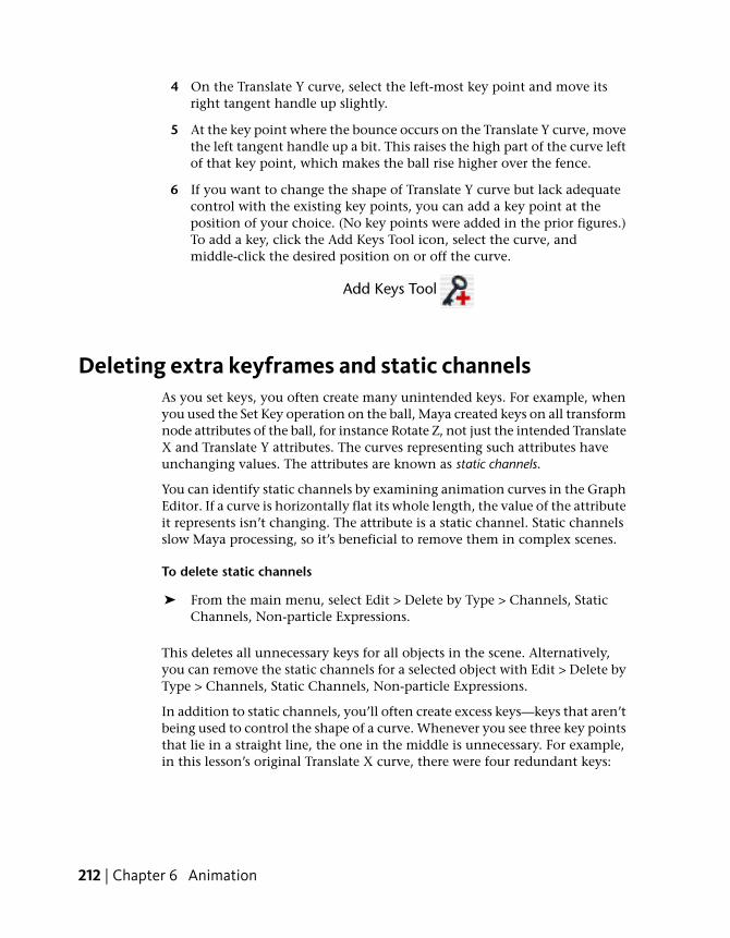
4 On the Translate Y curve, select the left-most key point and move itsright tangent handle up slightly.
5 At the key point where the bounce occurs on the Translate Y curve, movethe left tangent handle up a bit. This raises the high part of the curve leftof that key point, which makes the ball rise higher over the fence.
6 If you want to change the shape of Translate Y curve but lack adequatecontrol with the existing key points, you can add a key point at theposition of your choice. (No key points were added in the prior figures.)To add a key, click the Add Keys Tool icon, select the curve, andmiddle-click the desired position on or off the curve.
Deleting extra keyframes and static channelsAs you set keys, you often create many unintended keys. For example, whenyou used the Set Key operation on the ball, Maya created keys on all transformnode attributes of the ball, for instance Rotate Z, not just the intended TranslateX and Translate Y attributes. The curves representing such attributes haveunchanging values. The attributes are known as static channels.
You can identify static channels by examining animation curves in the GraphEditor. If a curve is horizontally flat its whole length, the value of the attributeit represents isn’t changing. The attribute is a static channel. Static channelsslow Maya processing, so it’s beneficial to remove them in complex scenes.
To delete static channels
➤ From the main menu, select Edit > Delete by Type > Channels, StaticChannels, Non-particle Expressions.
This deletes all unnecessary keys for all objects in the scene. Alternatively,you can remove the static channels for a selected object with Edit > Delete byType > Channels, Static Channels, Non-particle Expressions.
In addition to static channels, you’ll often create excess keys—keys that aren’tbeing used to control the shape of a curve. Whenever you see three key pointsthat lie in a straight line, the one in the middle is unnecessary. For example,in this lesson’s original Translate X curve, there were four redundant keys:
212 | Chapter 6 Animation
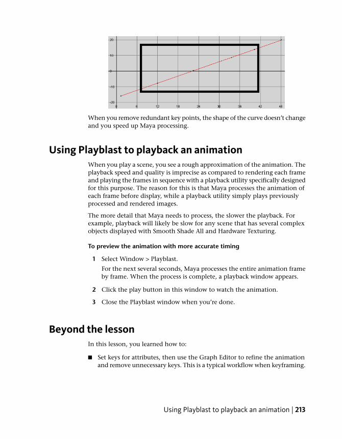
When you remove redundant key points, the shape of the curve doesn’t changeand you speed up Maya processing.
Using Playblast to playback an animationWhen you play a scene, you see a rough approximation of the animation. Theplayback speed and quality is imprecise as compared to rendering each frameand playing the frames in sequence with a playback utility specifically designedfor this purpose. The reason for this is that Maya processes the animation ofeach frame before display, while a playback utility simply plays previouslyprocessed and rendered images.
The more detail that Maya needs to process, the slower the playback. Forexample, playback will likely be slow for any scene that has several complexobjects displayed with Smooth Shade All and Hardware Texturing.
To preview the animation with more accurate timing
1 Select Window > Playblast.
For the next several seconds, Maya processes the entire animation frameby frame. When the process is complete, a playback window appears.
2 Click the play button in this window to watch the animation.
3 Close the Playblast window when you’re done.
Beyond the lessonIn this lesson, you learned how to:
■ Set keys for attributes, then use the Graph Editor to refine the animationand remove unnecessary keys. This is a typical workflow when keyframing.
Using Playblast to playback an animation | 213

You can animate most any attribute in Maya, not just the Translate, Rotate,and Scale attributes of a surface. For example, you can animate the intensityof a light, the transparency of a surface, the rotation of a camera view, orthe position of CVs.
■ Work with the Graph Editor to adjust the animation attributes animationcurves directly.The Graph Editor is the best tool for editing keyed animation by reshapinganimation curves. You can use it to change key positions, add or removekeys, and alter the fluidity and symmetry of animation.
Each key point on an animation curve has a Tangent setting that specifiesthe curvature leading into that point. The default Tangent setting (Spline)creates rounded curvature—useful for animating attributes that changesmoothly over time. The Linear setting creates angular curvature, usefulfor a bounce effect or any other abrupt change in attribute value. OtherTangent settings are available for different animation effects. For example,a Stepped setting lets you make an instantaneous leap in value, usefulwhen you want to flash a light off and on.
■ Use the Time and Range slider to play back your animation.Although the Graph Editor is a popular animation tool, you can also cut,copy, paste, and delete keys directly in the Time Slider to edit animation.Select a key position in the Time Slider, then right-click to select the desiredoperation from a pop-up menu.
You may find the following techniques useful when keyframing youranimations:
■ There are alternative object display modes that quicken the display ofanimation in the scene view. When you select Shading > Bounding Box(from the panel menu in the scene view), Maya displays simple box-shapedgeometry in place of the actual objects in your scene. The simpler shapesenable Maya to respond to any camera and object movement faster. Thedrawback is that you cannot edit the shape of the objects in this displaymode.
■ It is generally a recommended practice to animate a parent (group) noderather than objects themselves. By animating a parent node, you can avoidproblems that occur when the animation of one object in a hierarchyconflicts with the animation in another part of the hierarchy.
214 | Chapter 6 Animation

Lesson 2: Set Driven Key
IntroductionWith keyframe animation, you key an attribute value to a time in the TimeSlider. You repeat this process with different values at different times to animatethe object.
When you must animate multiple objects or attributes that interrelate, settingkeyframes can quickly become a complex task. Set Driven Key is a techniquefor driving one object’s or attribute’s animation from another attribute.
With driven keys, you relate an attribute value to the value of another attribute.You repeat this with different values to create a dependent link between a pairof attributes. A change in the driver attribute alters the value of the drivenattribute. In this way the animation of the driven attribute doesn’t need tobe manually set; it occurs automatically once the relationship betweenattributes has been established. This makes setting up some types of animationsmuch more efficient. For example, you can use driven keys to make a dooropen when a character walks in front of it.
In this lesson, you will learn how to use Set Driven Key in order to animate adoor rising upwards when a ball approaches it.
In this lesson you learn how to:
■ Link the object attribute behavior between two objects which will link themovement of one keyframed object to another with no keyframes assigned.
■ Use the Graph Editor to adjust the animation for the driven object.
Lesson setupIn the following steps, you set a playback range that’s long enough to see theanimation clearly. You also create the ball and the door, and position themin the scene view in preparation for the animation.
Lesson 2: Set Driven Key | 215
1 Make sure you’ve done the steps in Preparing for the lessons on page 199.
2 Create a new scene.
3 Go to the start frame.
4 Create a polygonal cube and name it Door.
5 Scale and position it roughly as shown in the previous figure. Have thebottom edge of the door lie roughly along the X-axis.
6 With the pointer in the perspective view, press 5 (for Shading > SmoothShade All).
7 Create a small polygonal sphere and name it Ball. Scale and position itroughly as shown in the prior figure in the introduction. Have it sitroughly at 0, 1, 10 (X, Y, Z).
Use the default color for the door and the ball.
Using Set Driven Key to link attributesThe following steps link the door’s movement to the ball’s movement usingSet Driven Key.
To link the door’s movement to the ball’s movement
1 Select the door and choose Animate > Set Driven Key > Set.
The Set Driven Key window appears with the door in the Driven list.
216 | Chapter 6 Animation

2 Click translateY in the Driven list.
This is the attribute to be driven by the ball’s movement.
3 Select the ball in the scene view.
4 In the Set Driven Key window, click the Load Driver button.
The ball appears in the Driver list.
5 In the Set Driven Key window, click translateZ in the Driver list.
This is the attribute that will drive the door’s movement.
You can set a driven key only after you select an attribute in the Driverlist and in the Driven list.
6 In the Set Driven Key window, click Key.
This sets a driven key relationship that links the current Translate Z valueof the ball to the current Translate Y value of the door. Whenever theball’s Translate Z is at this position, the door’s Translate Y will be at itscurrent position.
Using Set Driven Key to link attributes | 217

The Time Slider is not involved in a driven key relationship and displaysno red markers for keys.
7 Move the ball to the door’s position and then move the door above theball.
8 In the Set Driven Key window, click Key.
This sets another driven key that links the current Translate Z value ofthe ball to the Translate Y value of the door.
9 Move the ball to the right of the door and then lower the door to itsprevious position as shown in the following figure.
10 In the Set Driven Key window, click Key.
This sets another driven key that links the attributes.
You’ve set three driven keys that link the attribute values at differentpositions. Maya interpolates the linked values to generate the valuesbetween the keys.
If you drag the ball toward the door from either side, the door risessmoothly.
Playing back the animation from the Time Slider doesn’t move the ballor the door. Driven keys link one attribute to another. They don’t linkattributes to times in the Time Slider. However, if you were to animatethe movement of the ball, the door would move based on the driven keyrelationship that has been set.
218 | Chapter 6 Animation

Viewing the results in the Graph EditorIn the next steps you’ll examine the animation curve resulting from the drivenkeys you’ve set. If you are unfamiliar with animation curves and the GraphEditor, see Lesson 1: Keyframes and the Graph Editor on page 200.
To view the set driven key results in the Graph Editor
1 Select the door. To display the animation curve for a driven key in theGraph Editor, you must select the object containing the driven attribute,not the object containing the driving attribute.
2 Select Window > Animation Editors > Graph Editor.
3 From the Graph Editor, select View > Frame All. The Graph Editor showsthe driven keys that link the door’s TranslateY value to the ball’s TranslateZ value. An example follows:
The column of numbers on the left lists the driven attribute values. Therow at the bottom lists driver attribute values. The animation curve showsthe relationship between the values—the door’s Translate Y value risesas the ball’s Translate Z value approaches 0.
You can use the Graph Editor to edit the shape of the curve to make thedoor rise faster, slower, and higher as the ball approaches it.
Beyond the lessonIn this lesson you learned how to:
■ Set driven keys to link one attribute’s values to another.A driven attribute is not directly affected when you play the animation.It is linked to a driving attribute’s value, not animation time. However,you can use regular animation keys, expressions, motion paths, or other
Viewing the results in the Graph Editor | 219
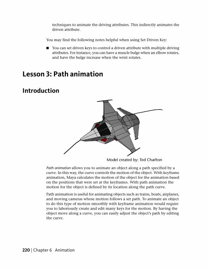
techniques to animate the driving attributes. This indirectly animates thedriven attribute.
You may find the following notes helpful when using Set Driven Key:
■ You can set driven keys to control a driven attribute with multiple drivingattributes. For instance, you can have a muscle bulge when an elbow rotates,and have the bulge increase when the wrist rotates.
Lesson 3: Path animation
Introduction
Path animation allows you to animate an object along a path specified by acurve. In this way, the curve controls the motion of the object. With keyframeanimation, Maya calculates the motion of the object for the animation basedon the positions that were set at the keyframes. With path animation themotion for the object is defined by its location along the path curve.
Path animation is useful for animating objects such as trains, boats, airplanes,and moving cameras whose motion follows a set path. To animate an objectto do this type of motion smoothly with keyframe animation would requireyou to laboriously create and edit many keys for the motion. By having theobject move along a curve, you can easily adjust the object’s path by editingthe curve.
220 | Chapter 6 Animation
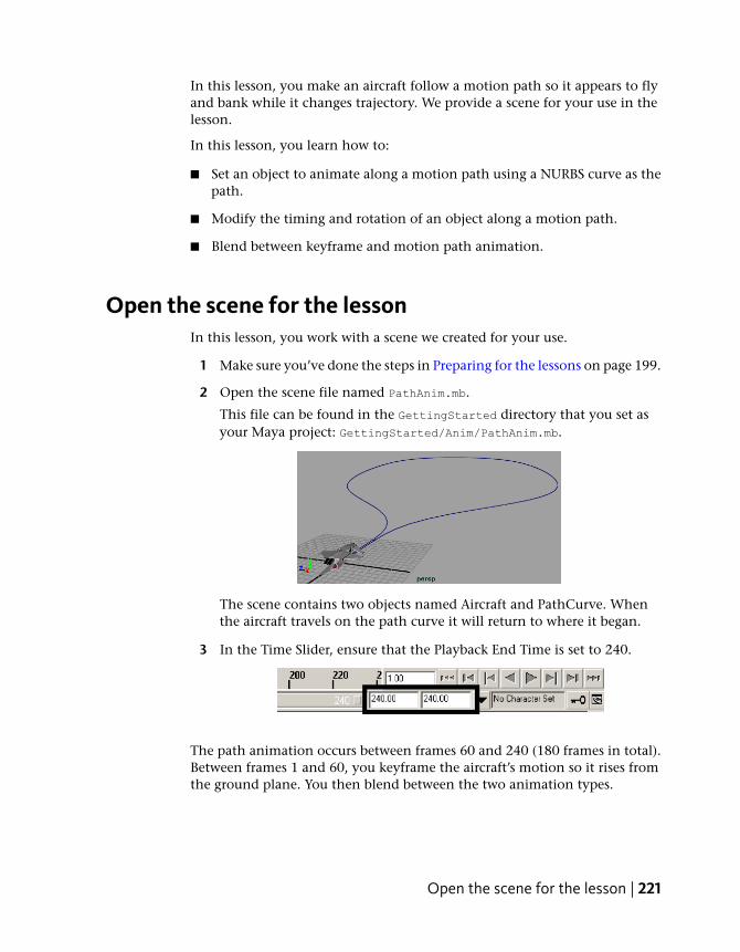
In this lesson, you make an aircraft follow a motion path so it appears to flyand bank while it changes trajectory. We provide a scene for your use in thelesson.
In this lesson, you learn how to:
■ Set an object to animate along a motion path using a NURBS curve as thepath.
■ Modify the timing and rotation of an object along a motion path.
■ Blend between keyframe and motion path animation.
Open the scene for the lessonIn this lesson, you work with a scene we created for your use.
1 Make sure you’ve done the steps in Preparing for the lessons on page 199.
2 Open the scene file named PathAnim.mb.
This file can be found in the GettingStarted directory that you set asyour Maya project: GettingStarted/Anim/PathAnim.mb.
The scene contains two objects named Aircraft and PathCurve. Whenthe aircraft travels on the path curve it will return to where it began.
3 In the Time Slider, ensure that the Playback End Time is set to 240.
The path animation occurs between frames 60 and 240 (180 frames in total).Between frames 1 and 60, you keyframe the aircraft’s motion so it rises fromthe ground plane. You then blend between the two animation types.
Open the scene for the lesson | 221

Animating an object along a motion pathTo animate the aircraft along the path curve, first select the aircraft and thepath curve and then set appropriate options for the motion path animation.In the options window, you need to set the required time range for the pathanimation. You also need to ensure that the aircraft is oriented facing towardsthe direction of travel. The Follow, Front, and Up axis option settingsdetermine the aircraft’s orientation along the path.
To attach the aircraft to the motion path
1 Set the Time Slider to frame 1.
2 Select the aircraft and then shift-select the path curve.
3 In the main menu, select Animate > Motion Paths > Attach to Motion
Path > .
The Attach to Motion Path Options window appears.
4 In the options window, ensure the options are set as follows, then clickAttach:
■ Time Range: Start/End
■ Start Time: 60
■ End Time: 240
■ Follow: On
■ Front Axis: X
■ Up Axis: Y
■ World Up Type: Scene Up
■ Leave all other settings off
222 | Chapter 6 Animation
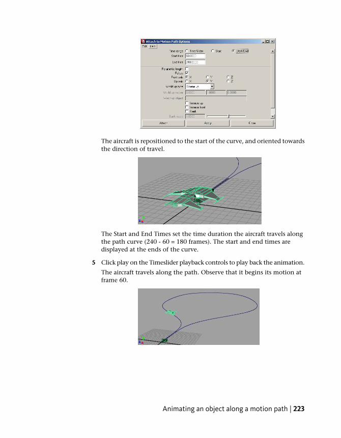
The aircraft is repositioned to the start of the curve, and oriented towardsthe direction of travel.
The Start and End Times set the time duration the aircraft travels alongthe path curve (240 - 60 = 180 frames). The start and end times aredisplayed at the ends of the curve.
5 Click play on the Timeslider playback controls to play back the animation.
The aircraft travels along the path. Observe that it begins its motion atframe 60.
Animating an object along a motion path | 223

Changing the timing of an object along a motion pathWhen you first assign an object to a motion path, by default, the object travelsalong the path at a constant speed. In this lesson, you want the aircraft toinitially travel along the path slowly, accelerate, and then finally move moreslowly when it nears the end of the motion path.
You can change the rate of travel for the aircraft by keyframing attributes thataffect where the aircraft is positioned on the curve at a given time.
To view the attributes for the motion path
1 Set the Time Slider to frame 1.
2 Select the aircraft.
3 Open the Channel Box by clicking the Show/Hide Channel Box icon onthe Status Line.
4 In the Channel Box, click on the word motionPath1 that appears in theAircraft’s Inputs list.
The attributes for motionPath1 appear at the bottom of the Inputs list.(Scroll the Channel Box window if the MotionPath1 attributes are notfully visible).
The UValue attribute controls where the aircraft gets positioned along thecurve. The UValue refers to the curves parameterization. Parameterization is amethod used by Maya to divide a curve into increments of known amountsso that a location along the curve can be determined.
224 | Chapter 6 Animation
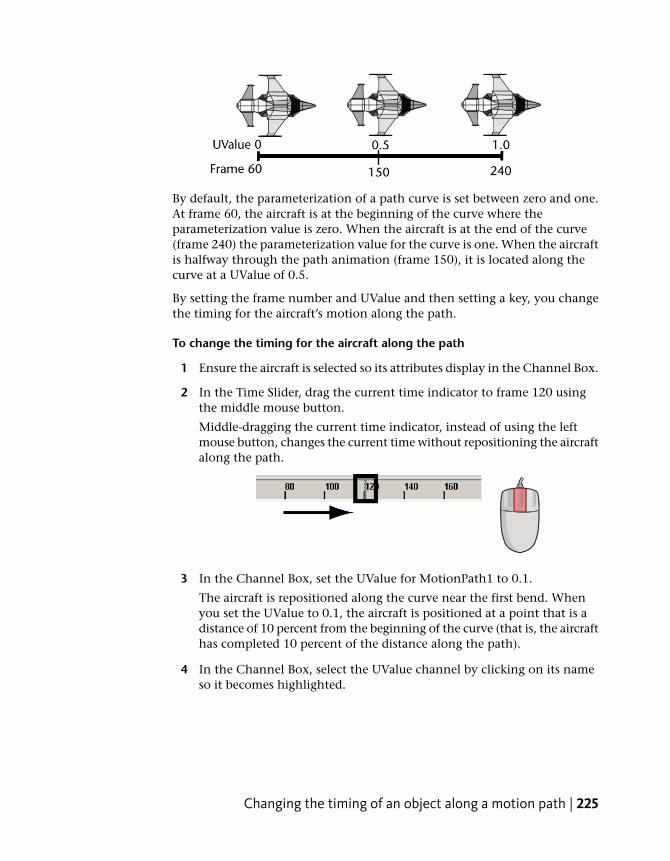
By default, the parameterization of a path curve is set between zero and one.At frame 60, the aircraft is at the beginning of the curve where theparameterization value is zero. When the aircraft is at the end of the curve(frame 240) the parameterization value for the curve is one. When the aircraftis halfway through the path animation (frame 150), it is located along thecurve at a UValue of 0.5.
By setting the frame number and UValue and then setting a key, you changethe timing for the aircraft’s motion along the path.
To change the timing for the aircraft along the path
1 Ensure the aircraft is selected so its attributes display in the Channel Box.
2 In the Time Slider, drag the current time indicator to frame 120 usingthe middle mouse button.
Middle-dragging the current time indicator, instead of using the leftmouse button, changes the current time without repositioning the aircraftalong the path.
3 In the Channel Box, set the UValue for MotionPath1 to 0.1.
The aircraft is repositioned along the curve near the first bend. Whenyou set the UValue to 0.1, the aircraft is positioned at a point that is adistance of 10 percent from the beginning of the curve (that is, the aircrafthas completed 10 percent of the distance along the path).
4 In the Channel Box, select the UValue channel by clicking on its nameso it becomes highlighted.
Changing the timing of an object along a motion path | 225
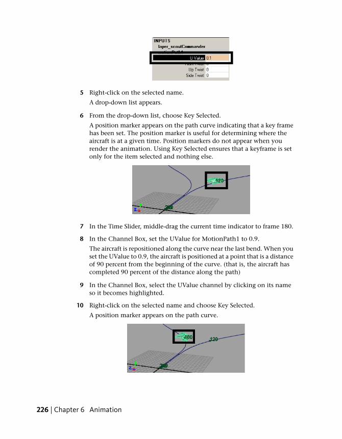
5 Right-click on the selected name.
A drop-down list appears.
6 From the drop-down list, choose Key Selected.
A position marker appears on the path curve indicating that a key framehas been set. The position marker is useful for determining where theaircraft is at a given time. Position markers do not appear when yourender the animation. Using Key Selected ensures that a keyframe is setonly for the item selected and nothing else.
7 In the Time Slider, middle-drag the current time indicator to frame 180.
8 In the Channel Box, set the UValue for MotionPath1 to 0.9.
The aircraft is repositioned along the curve near the last bend. When youset the UValue to 0.9, the aircraft is positioned at a point that is a distanceof 90 percent from the beginning of the curve. (that is, the aircraft hascompleted 90 percent of the distance along the path)
9 In the Channel Box, select the UValue channel by clicking on its nameso it becomes highlighted.
10 Right-click on the selected name and choose Key Selected.
A position marker appears on the path curve.
226 | Chapter 6 Animation

11 Click play on the Time Slider’s playback control to play back theanimation.
The motion of the aircraft is not smooth as it travels along the path. Itinitially moves forwards and backwards a bit at the beginning and endof the path. This indicates that some adjustment of the animation isrequired. You adjust the animation using the Graph Editor.
To view the Graph Editor
1 From the main menu, select Window > Animation Editors > Graph Editor.
The Graph Editor appears.
2 In the Graph Editor, select View > Frame All.
The Graph Editor updates to display the animation curve for the motionpath animation.
The shape of the animation curve provides some clues as to why the motionof the aircraft is not smooth. Between frames 60 and 84 the curve rises andthen drops slightly. Because the animation curve represents translation alongthe curve, a drop in the curve indicates that the object travels backwards. Asimilar occurrence happens at the end of the curve as well. To correct this,you need to modify the tangents for the keys in the Graph Editor.
To edit the tangents for the keys in the Graph Editor
1 In the Graph Editor, press the shift key, then double click on theanimation curve to select the four keys (frames 60, 120, 180 & 240)
2 In the Graph Editor menu, select Tangents > Linear.
Changing the timing of an object along a motion path | 227
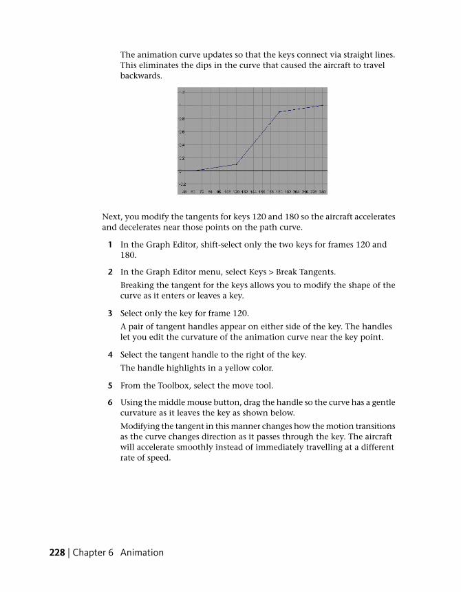
The animation curve updates so that the keys connect via straight lines.This eliminates the dips in the curve that caused the aircraft to travelbackwards.
Next, you modify the tangents for keys 120 and 180 so the aircraft acceleratesand decelerates near those points on the path curve.
1 In the Graph Editor, shift-select only the two keys for frames 120 and180.
2 In the Graph Editor menu, select Keys > Break Tangents.
Breaking the tangent for the keys allows you to modify the shape of thecurve as it enters or leaves a key.
3 Select only the key for frame 120.
A pair of tangent handles appear on either side of the key. The handleslet you edit the curvature of the animation curve near the key point.
4 Select the tangent handle to the right of the key.
The handle highlights in a yellow color.
5 From the Toolbox, select the move tool.
6 Using the middle mouse button, drag the handle so the curve has a gentlecurvature as it leaves the key as shown below.
Modifying the tangent in this manner changes how the motion transitionsas the curve changes direction as it passes through the key. The aircraftwill accelerate smoothly instead of immediately travelling at a differentrate of speed.
228 | Chapter 6 Animation

7 Select the key for frame 180.
8 Select the handle to the left of the key.
The handle highlights in blue.
9 Using the middle mouse button, drag the handle so the curve has a gentlecurvature as it enters the key as shown below.
Modifying this tangent for this key will cause the aircraft to deceleratesmoothly near the end of its travel.
The modified animation curve appears as shown below.
10 Close the Graph Editor.
11 Click play on the Time Slider’s playback control to play back theanimation.
Changing the timing of an object along a motion path | 229
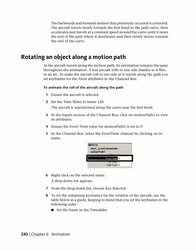
The backwards and forwards motion that previously occurred is corrected.The aircraft travels slowly towards the first bend in the path curve, thenaccelerates and travels at a constant speed around the curve until it nearsthe end of the path where it decelerates and then slowly moves towardsthe end of the curve.
Rotating an object along a motion pathAs the aircraft travels along the motion path, its orientation remains the samethroughout the animation. A real aircraft rolls to one side (banks) as it fliesin an arc. To make the aircraft roll to one side as it travels along the path youset keyframes for the Twist attributes in the Channel Box.
To animate the roll of the aircraft along the path
1 Ensure the aircraft is selected.
2 Set the Time Slider to frame 120.
The aircraft is repositioned along the curve near the first bend.
3 In the Inputs section of the Channel Box, click on motionPath1 to viewits attributes.
4 Ensure the Front Twist value for motionPath1 is set to 0.
5 In the Channel Box, select the FrontTwist channel by clicking on itsname.
6 Right-click on the selected name.
A drop-down list appears.
7 From the drop-down list, choose Key Selected.
8 To set the remaining keyframes for the rotation of the aircraft, use thetable below as a guide, keeping in mind that you set the keyframes in thefollowing order:
■ Set the frame in the Timeslider
230 | Chapter 6 Animation
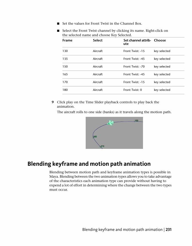
■ Set the values for Front Twist in the Channel Box.
■ Select the Front Twist channel by clicking its name. Right-click onthe selected name and choose Key Selected.
ChooseSet channel attrib-ute
SelectFrame
key selectedFront Twist: -15Aircraft130
key selectedFront Twist: -45Aircraft135
key selectedFront Twist: -70Aircraft150
key selectedFront Twist: -45Aircraft165
key selectedFront Twist: -15Aircraft170
key selectedFront Twist: 0Aircraft180
9 Click play on the Time Slider playback controls to play back theanimation.
The aircraft rolls to one side (banks) as it travels along the motion path.
Blending keyframe and motion path animationBlending between motion path and keyframe animation types is possible inMaya. Blending between the two animation types allows you to take advantageof the characteristics each animation type can provide without having toexpend a lot of effort in determining where the change between the two typesmust occur.
Blending keyframe and motion path animation | 231

In the steps that follow, you keyframe the aircraft to rise vertically from thefloor surface and then travel along the motion path by blending between thetwo animation types. To accomplish this, you do the following:
■ Move the motion path up above the ground plane.
■ Keyframe the aircraft so it rises vertically above the ground plane.
■ Blend between the keyframe and motion path animations.
To move the motion path
1 In the scene view, select only the path curve.
2 In the Channel Box, set Translate Y to 5 for PathCurve.
The path curve is repositioned above the ground plane in the scene view.The aircraft moves with the path curve because it is attached to the motionpath.
To keyframe the motion for the aircraft
1 Select only the aircraft.
2 Set the Timeslider to frame 1.
3 In the Channel Box, set the following for the aircraft:
■ Translate Y: 0
The aircraft is repositioned so it rests on the ground plane.
4 Select the Translate X, Y, and Z channels as well as the Rotate X, Y, andZ channels by click-dragging on their names so they become highlighted.
232 | Chapter 6 Animation
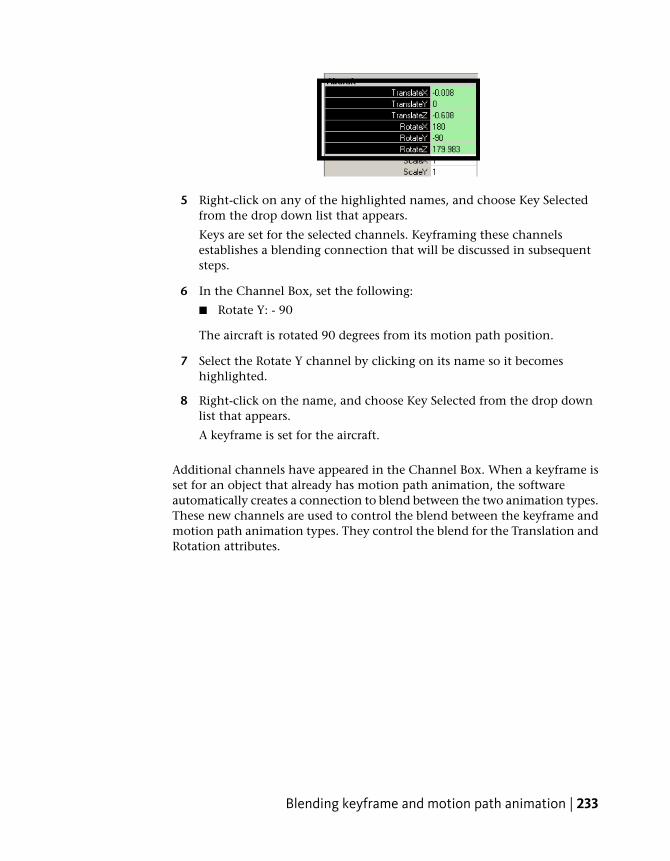
5 Right-click on any of the highlighted names, and choose Key Selectedfrom the drop down list that appears.
Keys are set for the selected channels. Keyframing these channelsestablishes a blending connection that will be discussed in subsequentsteps.
6 In the Channel Box, set the following:
■ Rotate Y: - 90
The aircraft is rotated 90 degrees from its motion path position.
7 Select the Rotate Y channel by clicking on its name so it becomeshighlighted.
8 Right-click on the name, and choose Key Selected from the drop downlist that appears.
A keyframe is set for the aircraft.
Additional channels have appeared in the Channel Box. When a keyframe isset for an object that already has motion path animation, the softwareautomatically creates a connection to blend between the two animation types.These new channels are used to control the blend between the keyframe andmotion path animation types. They control the blend for the Translation andRotation attributes.
Blending keyframe and motion path animation | 233

1 To set the remaining keyframes for the keyframe motion of the aircraft,use the table below as a guide, keeping in mind that you set the keyframesin the following order:
■ Set the frame in the Time Slider.
■ Set the Translate and Rotate values in the Channel Box.
■ Select only the channels for those values. Right-click on the selectedname and choose Key Selected.
ChooseSet channel attrib-ute
SelectFrame
key selectedTranslate Y: 1Aircraft20
key selectedTranslate Y: 2Aircraft30
key selectedRotate Z: 170Aircraft30
key selectedTranslate Y: 3Aircraft40
key selectedRotate Z: 170Aircraft40
2 Click play on the Timeslider playback controls to play back the animation.
The aircraft rises above the ground plane and then stops at frame 40.
234 | Chapter 6 Animation
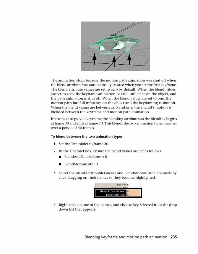
The animation stops because the motion path animation was shut off whenthe blend attribute was automatically created when you set the first keyframe.The blend attribute values are set to zero by default. When the blend valuesare set to zero, the keyframe animation has full influence on the object, andthe path animation is shut off. When the blend values are set to one, themotion path has full influence on the object and the keyframing is shut off.When the blend values are between zero and one, the aircraft’s motion isblended between the keyframe and motion path animation.
In the next steps, you keyframe the blending attributes so the blending beginsat frame 30 and ends at frame 70. This blends the two animation types togetherover a period of 40 frames.
To blend between the two animation types
1 Set the Timeslider to frame 30.
2 In the Channel Box, ensure the blend values are set as follows:
■ BlendAddDoubleLinear: 0
■ BlendMotionPath: 0
3 Select the BlendAddDoubleLinear1 and BlendMotionPath1 channels byclick-dragging on their names so they become highlighted.
4 Right-click on one of the names, and choose Key Selected from the dropdown list that appears.
Blending keyframe and motion path animation | 235
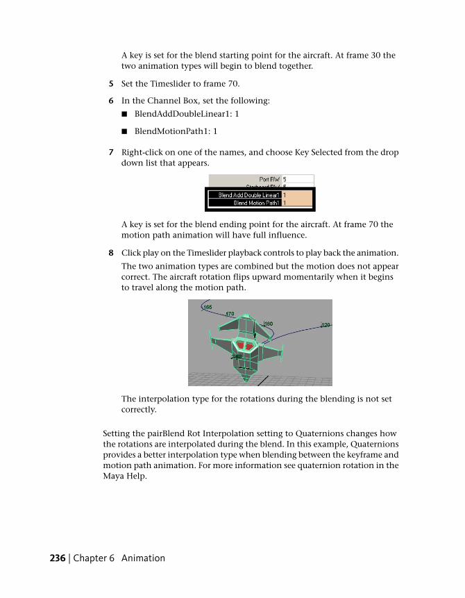
A key is set for the blend starting point for the aircraft. At frame 30 thetwo animation types will begin to blend together.
5 Set the Timeslider to frame 70.
6 In the Channel Box, set the following:
■ BlendAddDoubleLinear1: 1
■ BlendMotionPath1: 1
7 Right-click on one of the names, and choose Key Selected from the dropdown list that appears.
A key is set for the blend ending point for the aircraft. At frame 70 themotion path animation will have full influence.
8 Click play on the Timeslider playback controls to play back the animation.
The two animation types are combined but the motion does not appearcorrect. The aircraft rotation flips upward momentarily when it beginsto travel along the motion path.
The interpolation type for the rotations during the blending is not setcorrectly.
Setting the pairBlend Rot Interpolation setting to Quaternions changes howthe rotations are interpolated during the blend. In this example, Quaternionsprovides a better interpolation type when blending between the keyframe andmotion path animation. For more information see quaternion rotation in theMaya Help.
236 | Chapter 6 Animation
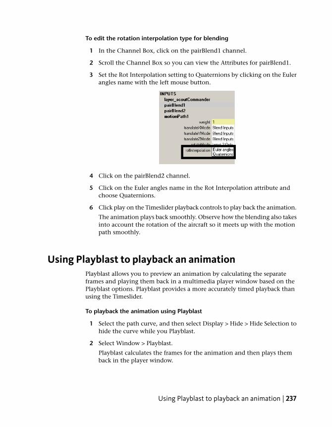
To edit the rotation interpolation type for blending
1 In the Channel Box, click on the pairBlend1 channel.
2 Scroll the Channel Box so you can view the Attributes for pairBlend1.
3 Set the Rot Interpolation setting to Quaternions by clicking on the Eulerangles name with the left mouse button.
4 Click on the pairBlend2 channel.
5 Click on the Euler angles name in the Rot Interpolation attribute andchoose Quaternions.
6 Click play on the Timeslider playback controls to play back the animation.
The animation plays back smoothly. Observe how the blending also takesinto account the rotation of the aircraft so it meets up with the motionpath smoothly.
Using Playblast to playback an animationPlayblast allows you to preview an animation by calculating the separateframes and playing them back in a multimedia player window based on thePlayblast options. Playblast provides a more accurately timed playback thanusing the Timeslider.
To playback the animation using Playblast
1 Select the path curve, and then select Display > Hide > Hide Selection tohide the curve while you Playblast.
2 Select Window > Playblast.
Playblast calculates the frames for the animation and then plays themback in the player window.
Using Playblast to playback an animation | 237

You have completed this lesson.
Beyond the lessonIn this lesson you learned how to:
■ Create a motion path animation using a NURBS curve as the motion path.When you draw your own curves remember that a curve has a definedstart and an end point based on how you create it. If your object is initiallypositioned at the wrong end of the curve, you can reverse the direction ofthe curve by setting the Menu Set to Modeling and then selecting EditCurves > Reverse Curve Direction.
If your objects are not oriented correctly on the path initially, you canchange the options in the Attach to Motion Path Options window. SeeAnimate > Motion Paths > Attach to Motion Path in the Maya Help.
■ Adjust the timing and rotation of an object when it travels along themotion path.In this lesson you were shown how to keyframe the roll (bank) of theaircraft. The Attach to Motion Path Options window provides an optioncalled Bank. The Bank option rotates an object as it travels around curvedportions of a motion path. It is useful for simple motion path animation.
■ Blend between keyframe and motion path animation types on the sameobject.For more information on how this works, see pairBlend in the Maya Help.
238 | Chapter 6 Animation

Lesson 4: Nonlinear animation with Trax
Introduction
Nonlinear animation allows you to create and edit an animation sequence byarranging smaller animation sequences (known as clips) on a timeline. A clipis a time-independent sequence of animation that you create from an existinganimation (keyframe animation, expressions, constraints, and motion capturedata - except motion path animation).
Nonlinear animation tools in Maya® TraxTM give you the ability to experimentwith your animation sequences and character animations without having toredo all of your work when you want to modify or construct a differentanimation.
Nonlinear animation is a non-destructive process. You can modify a particularclip’s attributes without affecting the source animation: the source materialremains untouched. This makes nonlinear animation useful when you wantto experiment, iterate, or change a particular animation sequence.
The primary tool for working with nonlinear animation is the Trax Editor.You can also store your clips for future use by creating a library of clips.
In this lesson you learn how to:
■ Key animation sequences for use as nonlinear clips in Trax.
Lesson 4: Nonlinear animation with Trax | 239

■ Create clips from your animation sequences for use in the Trax Editor.
■ Use the Trax editor to position, modify, and arrange clips in order to createand modify animation sequences in the scene.
■ Scale clips to modify the timing of an animation sequence.
■ Trim clips to remove unwanted motion.
■ Cycle clips to create motion that repeats.
■ Use the Graph Editor to modify the animation of a clip.
■ Use the Trax Editor to work with motion capture data.
■ Reuse clips using the Outliner and the Visor.
Open the first scene for the lessonThis lesson is presented in two parts. You work with two separate scene fileswe’ve created for your use. In the first part of this lesson, you learn some ofthe fundamental techniques for working with clips in the Trax Editor byanimating an aircraft taking off and landing.
1 Make sure you’ve done the steps in Preparing for the lessons on page 199.
2 Open the scene file named Trax_Lesson1.mb.
This file can be found in the GettingStarted directory that you set asyour Maya project: GettingStarted/Anim/Trax_Lesson1.mb.
The scene contains a model of an aircraft. For the first part of this lesson,you create and work with animation clips to control the motion of theaircraft.
3 In the Time Slider, set the Playback range as follows:
■ Playback Start Time: 1
240 | Chapter 6 Animation

■ Playback End Time: 240
To work more efficiently with the scene and the Trax Editor, you need to seta panel layout.
To set a panel layout for use with the Trax Editor
➤ From the perspective view’s menu, select Panels > Saved Layouts >Persp/Trax/Outliner.
The panel layout updates to display the Perspective view, Outliner, andTrax Editor simultaneously. This allows you to easily work with thesewindows without having to open and close them repeatedly.
Next, set the Outliner so it displays clips. The Outliner allows you to managethe various clips that get created with Trax.
To set the Outliner to display clips
1 In the Outliner menu, make sure that Display > DAG Objects Only isunchecked.
2 In the Outliner menu, select Show > Objects > Clips.
The Outliner displays an empty list until you create your first clip.
Open the first scene for the lesson | 241
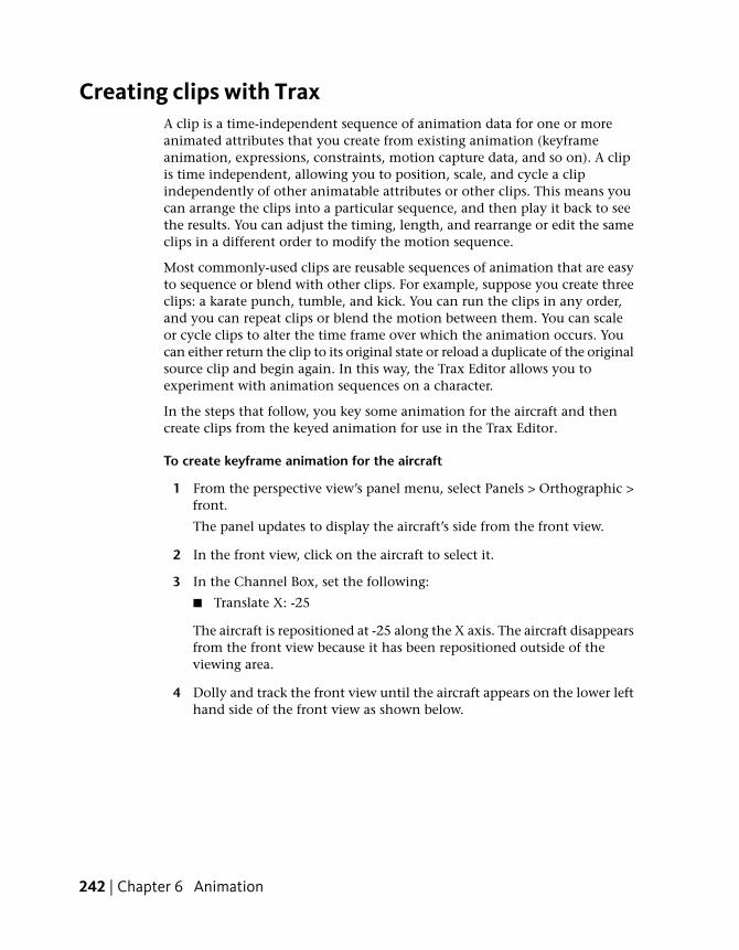
Creating clips with TraxA clip is a time-independent sequence of animation data for one or moreanimated attributes that you create from existing animation (keyframeanimation, expressions, constraints, motion capture data, and so on). A clipis time independent, allowing you to position, scale, and cycle a clipindependently of other animatable attributes or other clips. This means youcan arrange the clips into a particular sequence, and then play it back to seethe results. You can adjust the timing, length, and rearrange or edit the sameclips in a different order to modify the motion sequence.
Most commonly-used clips are reusable sequences of animation that are easyto sequence or blend with other clips. For example, suppose you create threeclips: a karate punch, tumble, and kick. You can run the clips in any order,and you can repeat clips or blend the motion between them. You can scaleor cycle clips to alter the time frame over which the animation occurs. Youcan either return the clip to its original state or reload a duplicate of the originalsource clip and begin again. In this way, the Trax Editor allows you toexperiment with animation sequences on a character.
In the steps that follow, you key some animation for the aircraft and thencreate clips from the keyed animation for use in the Trax Editor.
To create keyframe animation for the aircraft
1 From the perspective view’s panel menu, select Panels > Orthographic >front.
The panel updates to display the aircraft’s side from the front view.
2 In the front view, click on the aircraft to select it.
3 In the Channel Box, set the following:
■ Translate X: -25
The aircraft is repositioned at -25 along the X axis. The aircraft disappearsfrom the front view because it has been repositioned outside of theviewing area.
4 Dolly and track the front view until the aircraft appears on the lower lefthand side of the front view as shown below.
242 | Chapter 6 Animation

5 Press s to set a keyframe.
In the Channel Box, the channels display in a different color. The colorchange indicates that the channels now have animation applied to them.
NOTE If you normally use the Auto Keyframe function, you must shut it offfor this lesson. For more information see Auto Key in the Maya Help.
6 In the Time Slider, set the current time indicator to frame 240.
7 In the Channel Box, set the following:
■ Translate X: 25
The aircraft is repositioned at 25 along the X axis (the right hand side ofthe current front view).
8 In the Channel Box, select the Translate X channel by clicking on thename.
The Translate X name becomes highlighted.
9 Right-click on the selected name and choose Key Selected from thedrop-down list that appears.
Key Selected sets a keyframe for only the selected attribute.
Confirm that the animation sequence works as expected in the steps thatfollow.
To playback the animation using the playback controls
1 Click play on the Time Slider’s playback control to play back theanimation.
Creating clips with Trax | 243

The aircraft travels from left to right in the front view.
2 Click stop on the Time Slider’s playback control.
Now that you have keyframed an animation sequence and confirmed that itworks, you can create an animation clip.
To create an animation clip of the keyframe animation
1 In the Trax Editor menu, with the aircraft still selected, select Create >
Animation Clip > .
2 In the Create Clip Options window, select Edit > Reset Settings, and thenclick on the Create Clip button.
The Outliner updates and lists two items: clip1 and clip1Source. If theclips do not display refer to To set the Outliner to display clips on page241
When you created the clip, two clips were generated: a regular clip and asource clip. The source clip contains the animation curves for the character(based on the keyed attributes that the clip was created from). The sourceclip is stored with the file and can only be accessed from the Visor orOutliner. Maya saves the source clip outside of the Trax Editor to protectthe original animation curves from being accidentally modified andensures you have an unmodified clip to revert back to.
A regular clip (referred to simply as a clip) contains the same informationas the source clip, and is placed in a track in the Trax timeline. It is thisregular clip that you work with and modify in Trax.
244 | Chapter 6 Animation
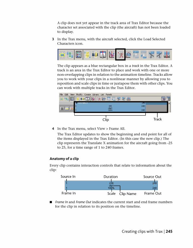
A clip does not yet appear in the track area of Trax Editor because thecharacter set associated with the clip (the aircraft) has not been loadedto display.
3 In the Trax menu, with the aircraft selected, click the Load SelectedCharacters icon.
The clip appears as a blue rectangular box in a track in the Trax Editor. Atrack is an area in the Trax Editor to place and work with one or morenon-overlapping clips in relation to the animation timeline. Tracks allowyou to work with your clips in a nonlinear manner by allowing you toreposition and scale clips in time or juxtapose them with other clips. Youcan work with multiple tracks in the Trax Editor.
4 In the Trax menu, select View > Frame All.
The Trax Editor updates to show the beginning and end point for all ofthe items displayed in the Trax Editor. (In this case the new clip.) Theclip represents the Translate X animation for the aircraft going from -25to 25, for a time range of 1 to 240 frames.
Anatomy of a clip
Every clip contains interaction controls that relate to information about theclip:
■ Frame In and Frame Out indicates the current start and end frame numbersfor the clip in relation to its position on the timeline.
Creating clips with Trax | 245
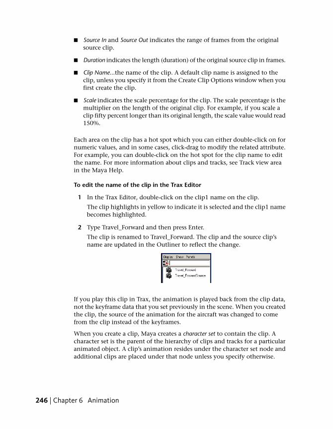
■ Source In and Source Out indicates the range of frames from the originalsource clip.
■ Duration indicates the length (duration) of the original source clip in frames.
■ Clip Name...the name of the clip. A default clip name is assigned to theclip, unless you specify it from the Create Clip Options window when youfirst create the clip.
■ Scale indicates the scale percentage for the clip. The scale percentage is themultiplier on the length of the original clip. For example, if you scale aclip fifty percent longer than its original length, the scale value would read150%.
Each area on the clip has a hot spot which you can either double-click on fornumeric values, and in some cases, click-drag to modify the related attribute.For example, you can double-click on the hot spot for the clip name to editthe name. For more information about clips and tracks, see Track view areain the Maya Help.
To edit the name of the clip in the Trax Editor
1 In the Trax Editor, double-click on the clip1 name on the clip.
The clip highlights in yellow to indicate it is selected and the clip1 namebecomes highlighted.
2 Type Travel_Forward and then press Enter.
The clip is renamed to Travel_Forward. The clip and the source clip’sname are updated in the Outliner to reflect the change.
If you play this clip in Trax, the animation is played back from the clip data,not the keyframe data that you set previously in the scene. When you createdthe clip, the source of the animation for the aircraft was changed to comefrom the clip instead of the keyframes.
When you create a clip, Maya creates a character set to contain the clip. Acharacter set is the parent of the hierarchy of clips and tracks for a particularanimated object. A clip’s animation resides under the character set node andadditional clips are placed under that node unless you specify otherwise.
246 | Chapter 6 Animation
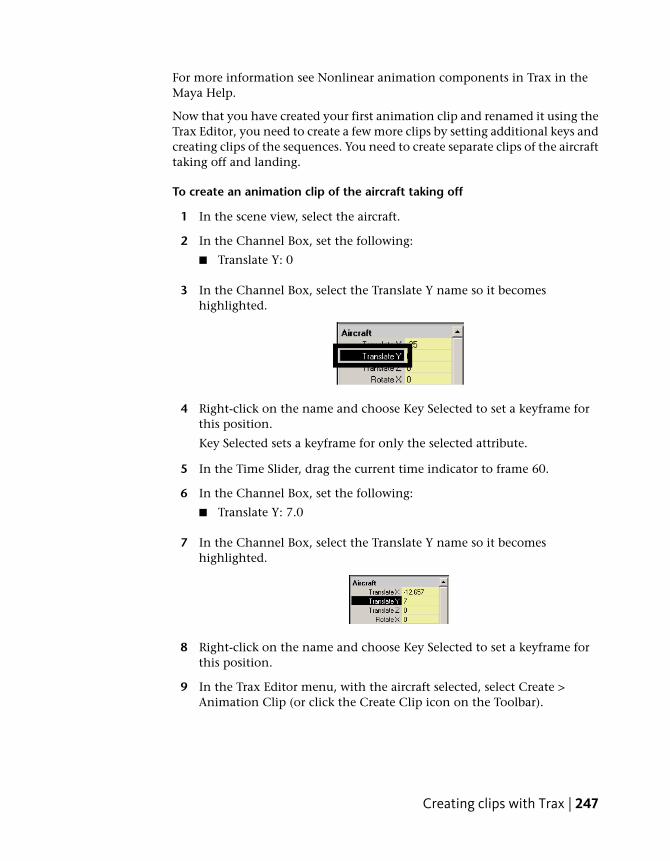
For more information see Nonlinear animation components in Trax in theMaya Help.
Now that you have created your first animation clip and renamed it using theTrax Editor, you need to create a few more clips by setting additional keys andcreating clips of the sequences. You need to create separate clips of the aircrafttaking off and landing.
To create an animation clip of the aircraft taking off
1 In the scene view, select the aircraft.
2 In the Channel Box, set the following:
■ Translate Y: 0
3 In the Channel Box, select the Translate Y name so it becomeshighlighted.
4 Right-click on the name and choose Key Selected to set a keyframe forthis position.
Key Selected sets a keyframe for only the selected attribute.
5 In the Time Slider, drag the current time indicator to frame 60.
6 In the Channel Box, set the following:
■ Translate Y: 7.0
7 In the Channel Box, select the Translate Y name so it becomeshighlighted.
8 Right-click on the name and choose Key Selected to set a keyframe forthis position.
9 In the Trax Editor menu, with the aircraft selected, select Create >Animation Clip (or click the Create Clip icon on the Toolbar).
Creating clips with Trax | 247

The Trax Editor updates to create an additional track and places the newclip on the new track. The Outliner updates to list the new clip and sourceclip.
10 In the Trax Editor, double-click on the new clip and rename it toAircraft_Rise.
11 Click play on the Time Slider’s playback control to play back theanimation.
The aircraft rises as it travels forward.
12 Click stop on the Time Slider’s playback control.
To create an animation clip of the aircraft landing
1 In the Timeslider, set the current time indicator to frame 180.
2 In the Channel Box, with the aircraft still selected, set Translate Y to 7.
3 In the Channel Box, select the Translate Y name so it becomeshighlighted.
4 Right-click on the name and choose Key Selected to set a keyframe forthis position.
5 In the Time Slider, set the current time indicator to frame 240.
6 In the Channel Box, set the Translate Y to 0.
248 | Chapter 6 Animation

7 In the Channel Box, select the Translate Y name so it becomeshighlighted.
8 Right-click on the name and choose Key Selected to set a keyframe forthis position.
9 Click play on the Time Slider playback controls to play back theanimation.
The aircraft travels forward and then lands as it nears the end of its travel.
10 Click stop on the Time Slider’s playback control.
11 In the Trax Editor menu, with the aircraft selected, select Create >Animation Clip.
The Trax Editor and Outliner update to show the new clip.
12 In the Trax Editor, double-click on the new clip and rename it toAircraft_Lower.
Changing the position of clips with TraxIt’s easy to alter the start time of clips to synchronize the action between clips.For example, the aircraft rises as it travels forward because the Travel_Forwardand Aircraft_Rise clips overlap in time. If you position the clips on theirrespective tracks so that one clip’s action occurs in the Trax timeline beforeor after the other, the motion occurs separately.
In this section, you learn how to reposition the clips so that the aircraft takesoff before it travels forward in X, and then have the aircraft land at the endof the sequence.
Changing the position of clips with Trax | 249

To change the position of a clip in a track
1 In the Trax Editor, move the mouse cursor over top of the Travel_Forwardclip.
When the mouse cursor is over top of a clip in the Trax Editor, the cursoricon changes to a pointer indicating that you can drag the clip to eitherside or up and down between tracks.
2 Click-drag the Travel_Forward clip horizontally to the right in its trackuntil the Frame In reads 60 as shown below.
3 Click play on the Time Slider playback controls to play back theanimation.
The aircraft takes off vertically, then travels to the right, and lands whileit is still travelling to the right. Because the two clips (Travel_Forwardand Aircraft_Rise) are positioned one after the other, the actions occurin a series versus simultaneously.
4 Click stop on the Time Slider’s playback control.
5 Click-drag the Aircraft_Lower clip horizontally to the right until thebeginning of the clip matches the end of the Travel_Forward clip on thetrack above it. (Frame In = 299)
If the view of the clips appears limited, select View > Frame All in theTrax Editor to resize the view to encompass the clips.
250 | Chapter 6 Animation

You also need to modify the Playback End Time because the animation timelineis longer as a result of repositioning the clips.
1 In the Time Slider, edit the Playback range as follows:
■ Playback End Time: 360
2 Click play on the Time Slider playback controls to play back theanimation.
The aircraft takes off vertically, then travels to the right, and then landsvertically once the Travel_Forward clip’s motion is complete. Because thethree clips are positioned end to end in relation to the timeline, theanimation occurs as a series of separate events.
3 Click stop on the Time Slider’s playback control.
Editing the animation of clipsYou can modify the animation of a clip using the Graph Editor in the sameway that you would modify any other type of animation. Because you areworking with the clip, and not the original animation, you won’t change theoriginal source clip animation.
In this section, you use the Graph Editor to modify the animation for eachclip so the aircraft’s motion accelerates and decelerates at the beginning andend of each clip.
To use the Graph Editor to modify a clip in Trax
1 Click on the Aircraft_Rise clip to select it.
Editing the animation of clips | 251

The selected clip highlights in yellow.
2 From the Trax menu, select View > Graph Anim Curves.
The Graph Editor appears.
3 In the Graph Editor, shift-select the two keys on the animation curve asshown below.
4 In the Graph Editor, select Tangents > Flat.
The shape of the animation curve updates to a gentle S-shape. Settingthe tangents for the animation curve in this manner modifies the clip’sanimation to cause the aircraft to accelerate when it first rises, anddecelerate when it nears the end of its vertical travel.
5 Repeat steps 1 through 4 to set the animation curve tangents in a similarmanner for the two remaining clips: Travel_Forward and Aircraft_Lower.
The shape of the animation curve for Aircraft_Lower will be reversed fromthe other clip curves because the motion is occurring in the oppositedirection.
6 Close the Graph Editor window.
7 Set the Time Slider’s current time indicator to frame 1.
8 Click play on the Time Slider’s playback control to play back theanimation.
The motion accelerates and decelerates at the beginning and end of eachclip. As a result, the motion appears more natural. It’s important to notethat the modified tangents for each clip are independent from the otheranimation clips and do not affect any other motion.
9 Click stop on the Time Slider’s playback control.
252 | Chapter 6 Animation

Reusing clips within TraxYou can save and reuse clips for future use. You can key specific types ofmotion or attribute effects, save them as clips, and reuse the clips for othercharacters.
When you reuse a clip created for one character and apply it to another, theclip attributes must be mapped to correspond between the two characters. Formore information, see Mapping animation between characters in the MayaHelp.
In this lesson, you work with clips created for this aircraft animation. Theclips contain animation to make the aircraft shift to the left and right andbank left and right.
To load a clip from disk
1 From the Trax menu, select File > Import Animation Clip.
The File Browser appears. When importing a clip, the File Browser defaultsto the clip directory of your current project.
2 Find the clip file named Bank_Left.ma in the GettingStarted/Anim/clipsdirectory.
3 Select the file named Bank_Left.ma and click the Import button.
The clip is imported and appears in the Outliner named asBank_LeftSource to indicate it is a source clip.
4 Repeat steps 1 and 2 to import the clips Bank_Right, Shift_Left andShift_Right.
When you have finished, four new clips appear in the Outliner as sourceclips. In the steps that follow, you place and position the clips on tracksin the Trax Editor.
NOTE When you import clips they also appear in, and can be accessed from,the Visor (Window > General Editors > Visor). The Visor is a graphical interfacethat allows you to import items that reside on disk or in your current file (such as files, textures, clips, or poses). Clips that are assigned to a characterin Trax will appear listed under the Character Clips tab in the Visor. Clips thathave not yet been placed on a track will appear listed in the Visor under theUnused Clips tab.
Reusing clips within Trax | 253

To place clips into a track from the Outliner
1 In the Outliner, using the middle mouse button drag the clip namedBank_LeftSource into the same track as the Rise and Lower clips. Ensureyou drag into an open area on the track that the clip will fit into.
2 Position the Bank_Left clip on the track so its Frame In number matchesthe Frame Out number on the Aircraft_Rise clip, as shown below.
3 Using the middle mouse button drag the clip named Bank_RightSourcefrom the Outliner into the same track as the Rise and Lower clips. Ensureyou drag into an open area on the track that the clip will fit into.
4 Position the Bank_Right clip on the track so its Frame In number matchesthe Frame Out number on the Bank_Left clip, as shown below.
You can also drag clips from the Outliner or Visor into the Trax Editor andcreate a new track for them to be placed in.
1 Drag the clip named Shift_Left1Source from the Outliner using the middlemouse button, but this time, drag to the narrow blue area above the tracksbefore releasing your middle mouse button.
254 | Chapter 6 Animation

A new track appears in the Trax Editor and the clip is placed on the newtrack.
The narrow blue box is the summary track for the character set (in thiscase the Aircraft) The summary track represents all of the clips under acharacter, subcharacter, or group. When you import a clip onto thesummary area by dragging it from the Outliner or Visor, the Trax Editorcreates a new track for the clip.
2 Click-drag the Shift_Left clip so it lies directly below the Bank_Left clipon the track above it.
Because the Shift_Left clip is positioned directly below the Bank_Left clip,the actions will occur simultaneously when the animation is played back.
3 Using the middle mouse button drag the clip named Shift_Right1Sourcefrom the Outliner into the same track as the Shift_Left clip . Ensure youdrag into an open area on the track.
4 Position the Shift_Right clip on the track so its Frame In number matchesthe Frame Out number on the Shift_Left clip, as shown below.
5 In the front view menu, select Panels > Perspective > persp.
The view updates to display the aircraft from a perspective view.
Reusing clips within Trax | 255
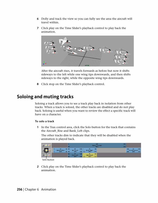
6 Dolly and track the view so you can fully see the area the aircraft willtravel within.
7 Click play on the Time Slider’s playback control to play back theanimation.
After the aircraft rises, it travels forwards as before but now it shiftssideways to the left while one wing tips downwards, and then shiftssideways to the right, while the opposite wing tips downwards.
8 Click stop on the Time Slider’s playback control.
Soloing and muting tracksSoloing a track allows you to see a track play back in isolation from othertracks. When a track is soloed, the other tracks are disabled and do not playback. Soloing is useful when you want to review the effect a specific track willhave on a character.
To solo a track
1 In the Trax control area, click the Solo button for the track that containsthe Aircraft_Rise and Bank_Left clips.
The other tracks dim to indicate that they will be disabled when theanimation is played back.
2 Click play on the Time Slider’s playback control to play back theanimation.
256 | Chapter 6 Animation

The aircraft rises, tilts left and right, and then lowers, without movingforward. Because the other tracks have been shut off temporarily, theaircraft’s motion is controlled by only one track.
3 Click stop on the Time Slider’s playback control.
4 Click the Solo button again to enable all the tracks.
The dimmed tracks become active again.
Muting a track disables only the selected track so it does not play back. Mutingis useful when you want to review the animation on one or more trackstogether without specific tracks being activated. You can mute one or moretracks.
To mute a track
1 In the Trax control area, click the Mute button for the track that containsthe Shift_Left and Shift_Right clips.
The muted track dims to indicate it is disabled.
2 Click play on the Time Slider’s playback control to play back theanimation.
The aircraft rises and tilts left and right as it travels forward, and thenlowers. Because the Shift_Left and Shift_Right track is temporarily muted,only the two remaining tracks affect the animation playback.
3 Click stop on the Time Slider’s playback control.
4 Unmute the track by clicking its mute button before proceeding to thenext section.
Scaling clips within TraxYou can scale single or multiple clips within the Trax Editor. Scaling a clipeither compresses or expands the animation of a clip so it occurs over a shorteror longer period of time. The resulting animation occurs faster or slower as aresult.
Scaling clips within Trax | 257

In the next steps, you select the four clips you imported to Trax, and scalethem together so they occur over the same time frame as the Travel_Forwardclip.
To scale multiple clips in the Trax Editor
1 In the Trax Editor, shift-click on the clips: Bank_Left, Bank_Right,Shift_Left1, and Shift_Right1.
The clip manipulator appears. The clip manipulator appears as a white boxthat encompasses the four clips with handles (triangles) on either endand a circle handle in the center. The clip manipulator allows you tomove or scale multiple clips.
2 Using the clip manipulator, click-drag the right-hand scale handle to theright until the Frame Out numbers on the Bank_Right and Shift_Rightclips match the Travel_Forward clip (Frame 299).
3 Click play on the Time Slider playback controls to play back theanimation.
When the aircraft travels, the sideways and banking motions occur overthe entire length of the Travel_Forward clip.
4 Click the stop button on the playback controls to stop the playback.
This completes the first half of the Trax lesson. In the second half of this lessonyou work with motion capture data in Trax.
258 | Chapter 6 Animation
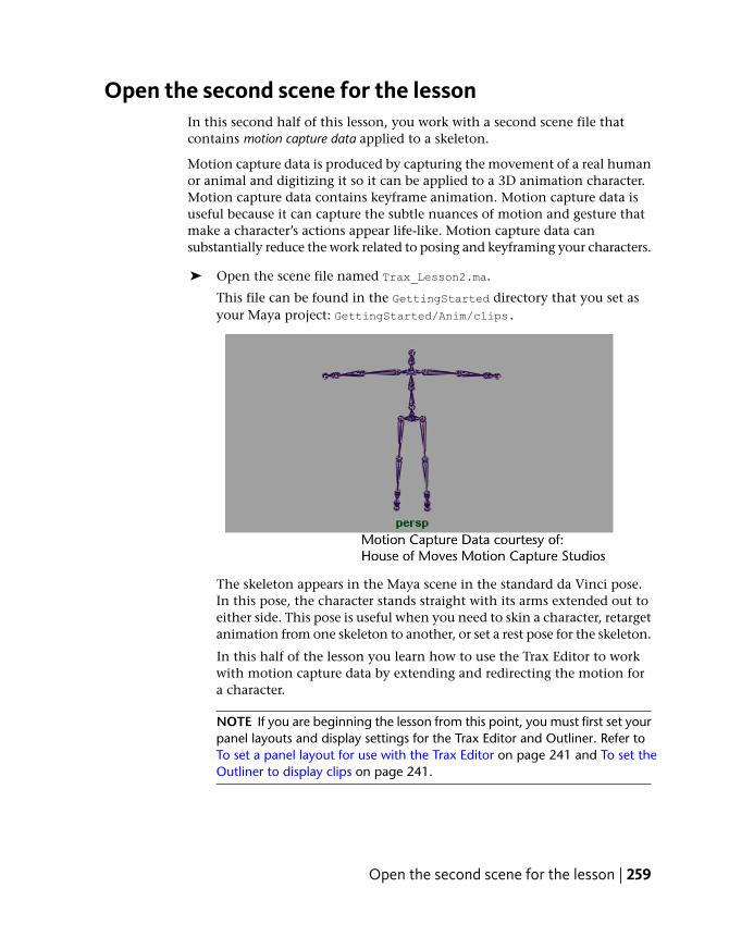
Open the second scene for the lessonIn this second half of this lesson, you work with a second scene file thatcontains motion capture data applied to a skeleton.
Motion capture data is produced by capturing the movement of a real humanor animal and digitizing it so it can be applied to a 3D animation character.Motion capture data contains keyframe animation. Motion capture data isuseful because it can capture the subtle nuances of motion and gesture thatmake a character’s actions appear life-like. Motion capture data cansubstantially reduce the work related to posing and keyframing your characters.
➤ Open the scene file named Trax_Lesson2.ma.
This file can be found in the GettingStarted directory that you set asyour Maya project: GettingStarted/Anim/clips.
The skeleton appears in the Maya scene in the standard da Vinci pose.In this pose, the character stands straight with its arms extended out toeither side. This pose is useful when you need to skin a character, retargetanimation from one skeleton to another, or set a rest pose for the skeleton.
In this half of the lesson you learn how to use the Trax Editor to workwith motion capture data by extending and redirecting the motion fora character.
NOTE If you are beginning the lesson from this point, you must first set yourpanel layouts and display settings for the Trax Editor and Outliner. Refer toTo set a panel layout for use with the Trax Editor on page 241 and To set theOutliner to display clips on page 241.
Open the second scene for the lesson | 259
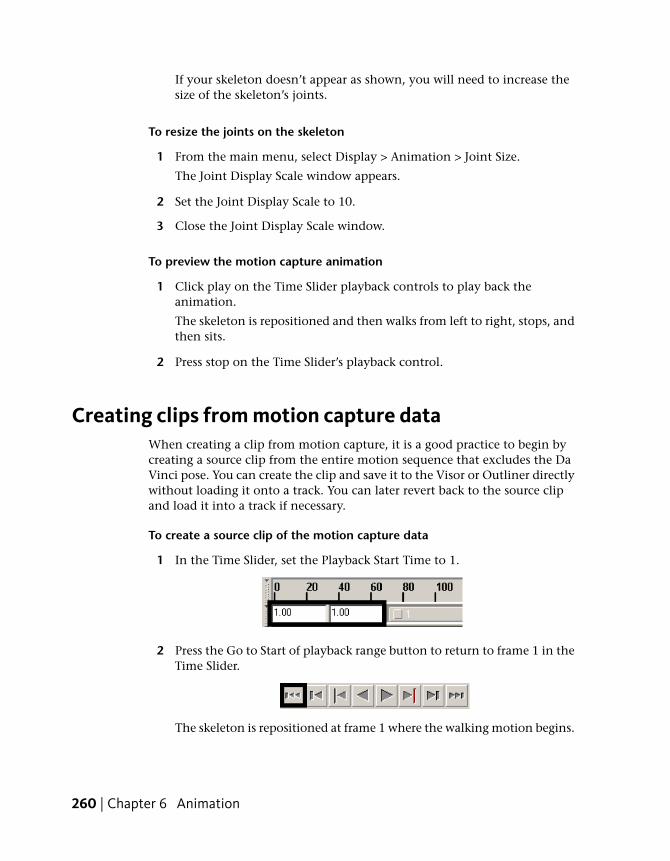
If your skeleton doesn’t appear as shown, you will need to increase thesize of the skeleton’s joints.
To resize the joints on the skeleton
1 From the main menu, select Display > Animation > Joint Size.
The Joint Display Scale window appears.
2 Set the Joint Display Scale to 10.
3 Close the Joint Display Scale window.
To preview the motion capture animation
1 Click play on the Time Slider playback controls to play back theanimation.
The skeleton is repositioned and then walks from left to right, stops, andthen sits.
2 Press stop on the Time Slider’s playback control.
Creating clips from motion capture dataWhen creating a clip from motion capture, it is a good practice to begin bycreating a source clip from the entire motion sequence that excludes the DaVinci pose. You can create the clip and save it to the Visor or Outliner directlywithout loading it onto a track. You can later revert back to the source clipand load it into a track if necessary.
To create a source clip of the motion capture data
1 In the Time Slider, set the Playback Start Time to 1.
2 Press the Go to Start of playback range button to return to frame 1 in theTime Slider.
The skeleton is repositioned at frame 1 where the walking motion begins.
260 | Chapter 6 Animation

3 In the persp view, select the skeleton by click-dragging a bounding boxaround the skeleton.
The skeleton is highlighted. When the skeleton is selected, many redticks appear in the Time Slider. The red ticks represent keyframes fromthe motion capture data.
4 In the Trax Editor menu, select Create > Animation Clip > .
The Create Clip Options window appears.
5 In the Create Clip Options window, click Edit > Reset Settings to set thetool to its default settings, and then set the following:
■ Type WalkSit in the Name field.
■ Keys - Leave Keys in Timeline: On
■ Put Clip in Visor Only: On
■ Click Create Clip.
The source clip appears in the Outliner named as WalkSitSource. (If youuse the Visor, the clip appears under the Character Clips tab.)
Extending the length of motion capture dataYou often need more animation of a motion sequence than is provided in themotion capture data. For example, you may need to have a walk cycle that issubstantially longer than what was provided in the original file. You can usethe Trax Editor to edit the motion capture data and create clips that can be
Extending the length of motion capture data | 261

cycled to make longer animation sequences. When you cycle a clip, the clip isextended in length with duplicate animation from the original clip over adefined interval of time.
If you want to cycle a clip, you must first determine areas within the animationsequence where the clip repeats seamlessly. For example, if you want to createa walk cycle from the motion capture data, you need to determine the time(frame) where the right foot is planted on the ground, and then move forwardin the Time Slider, frame by frame, until you find the next frame where theright foot is planted on the ground in exactly the same (or very similar)manner, and then create a clip. The resulting clip will contain two steps ofthe walking motion. The clip can then be cycled to produce a motion thatrepeats. How seamlessly it cycles depends on the original motion capture data.
In the steps that follow you create a walk cycle from the motion capture databy:
■ Creating a clip from the walking portion of the motion capture sequencethat can be repeated.
■ Cycle the clip to create a longer walk sequence.
To create a clip that can be cycled
1 In the Time Slider, drag the current time indicator to frame 6.
The skeleton updates in the scene to a walking pose where the right footis planted on the ground.
2 Drag the current time indicator forward in the Time Slider until you reachframe 45.
At frame 45, the skeleton is posed in a similar manner as it appeared atframe 6. If you use this range of frames (6 to 45), you can create a clipthat can be cycled.
3 In the persp view ensure the skeleton is selected.
4 In the Trax Editor menu, select Create > Animation Clip > .
The Create Clip Options window appears.
5 In the Create Clip Options window, click Edit > Reset Settings to set thetool to its default settings, and then set the following:
■ Type WalkCycle in the Name field.
■ Put Clip in Trax Editor and Visor: On
262 | Chapter 6 Animation
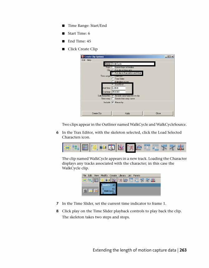
■ Time Range: Start/End
■ Start Time: 6
■ End Time: 45
■ Click Create Clip
Two clips appear in the Outliner named WalkCycle and WalkCycleSource.
6 In the Trax Editor, with the skeleton selected, click the Load SelectedCharacters icon.
The clip named WalkCycle appears in a new track. Loading the Characterdisplays any tracks associated with the character; in this case theWalkCycle clip.
7 In the Time Slider, set the current time indicator to frame 1.
8 Click play on the Time Slider playback controls to play back the clip.
The skeleton takes two steps and stops.
Extending the length of motion capture data | 263

9 Press stop on the playback controls to stop the playback and reset thecurrent time indicator to frame 1.
10 In the Trax Editor, drag the clip to the left in its track until the Frame Innumber reads 1.
This sets the clip to begin at frame 1 in the Time Slider.
In the steps that follow, you cycle the clip to extend the animation so theskeleton repeats the two step motion and travels farther in the scene.
To cycle the motion for the walk clip
1 In the Trax Editor, shift-drag the lower right corner of the Walk clip tothe right until a C2.0 number appears in the new region of the clip.
When you shift-drag over the Frame Out area, the mouse cursor changesto a circular pointing arrow to indicate you are cycling the clip.
2 Double-click on the cycled clip in the C2 region.
The region is highlighted to indicate you can edit the values in the region.The number will likely not be exactly 2.0. This means that the cycle willnot repeat exactly twice.
3 Type 2.0 to modify the clip so it cycles exactly twice.
264 | Chapter 6 Animation

4 With the clip selected in the Trax Editor, open the Attribute Editor. Openthe Channel Offsets menu and ensure that the WalkCycle clip’s root.scaleand root.translate offset attributes are set to Relative and root.rotate offsetattributes are set to Absolute.
Setting the offset attributes for the clip to Relative ensures that each cyclebegins at the position where the last sequence left off. This ensures thatthe skeleton doesn’t jump back to its start point after each cycle.
5 Click play on the Time Slider playback controls to play back the clip.
The skeleton takes six steps and then stops.
When the clip is cycled twice, the two-step walking motion occurs threetimes in total.
6 Press stop on the playback controls to stop the playback and reset thecurrent time indicator to frame 1.
Extending the length of motion capture data | 265

Redirecting the motion within a clipMotion capture data can be used in a variety of ways. You can redirect themotion of a character using the same motion capture data. The Redirect toolallows you to alter the original animation for a character by modifying itspath or orientation at any time during its animation. The Redirect tool doesthis by offsetting the translation and rotation attributes for the selectedcharacter.
For example, you can change the start or end point of a character’s animationby redirecting the character’s starting position or by redirecting its motionduring the animation. You can redirect a character in an existing animationsequence in the scene or a character associated with a clip within the TraxEditor.
In the steps that follow, you redirect the skeleton to turn to the right whilewalking. The workflow for the redirection is as follows:
■ Scrub forward in the animation to determine a location in the clip whereyou want the character to turn. A realistic choice is where the ball of theskeleton’s right foot is planted on the ground plane because this accuratelysimulates how a real person might turn.
■ Select the entire skeleton. In this example, selecting the entire skeletonselects it at the root joint (the top node of the skeleton’s hierarchy)Selecting at the root joint ensures that the entire skeleton gets redirectedwhen the redirection control is applied.
■ Create and position a rotation redirection control using the Redirect tool.
■ Keyframe an initial starting rotation for the redirection control.
■ Rotate the redirection control so the skeleton faces the new direction oftravel.
■ Keyframe the second rotation for the redirection control.
To create a redirection control for the skeleton
1 In the Time Slider, drag the current time indicator to frame 36.
This frame is where the ball of the skeleton’s right foot is planted on theground plane. Use this frame as the location where the skeleton will turnto the right.
2 Select the skeleton in the scene view by click-dragging a bounding boxaround it.
266 | Chapter 6 Animation

3 In the main menu, select Character > Redirect > .
4 In the Character Redirection Options Window set the Redirection Typeto Rotation only and then click the Redirect button.
A Rotation redirection control appears between the hips of the skeleton,where the root joint for the skeleton’s hierarchy is.
You want the skeleton to pivot (rotate) while standing on the ball of its rightfoot. To do this, you need to move the redirection control to the ball of theright foot of the skeleton.
To move the redirection control to the ball of the foot
1 From the Toolbox, select the Move tool.
The Move tool manipulator appears on the redirect manipulator.
2 Press the v key and click-drag the redirection control until it is locatedon the ball of the right foot as shown below.
Pressing the v key while using the Move Tool momentarily enables theSnap to Points tool.
Redirecting the motion within a clip | 267

The redirection control is now positioned to redirect the skeleton’s walkingmotion. To complete the redirection process, you need to set keyframes whilesetting the redirection control so the redirection of the skeleton can occur.
To keyframe the redirection control
1 With the redirection control selected, press s to set a keyframe.
A red tick appears in the Time Slider at frame 36 indicating the keyframe.Setting a keyframe establishes the starting rotation for the redirectionrotation of the skeleton.
2 In the Time Slider, drag the current time indicator to frame 57.
The skeleton updates to a position where its left foot is planted on theground plane. This is the location where you want the skeleton to berotated to its new direction of travel.
3 In the Channel Box, with the redirection control still selected, set theRotate Y attribute to -45.
4 Rotate the redirection control approximately -45 degrees about the Y axisuntil the skeleton is facing in the direction shown below. (You can usethe Channel Box values as a guide.)
268 | Chapter 6 Animation
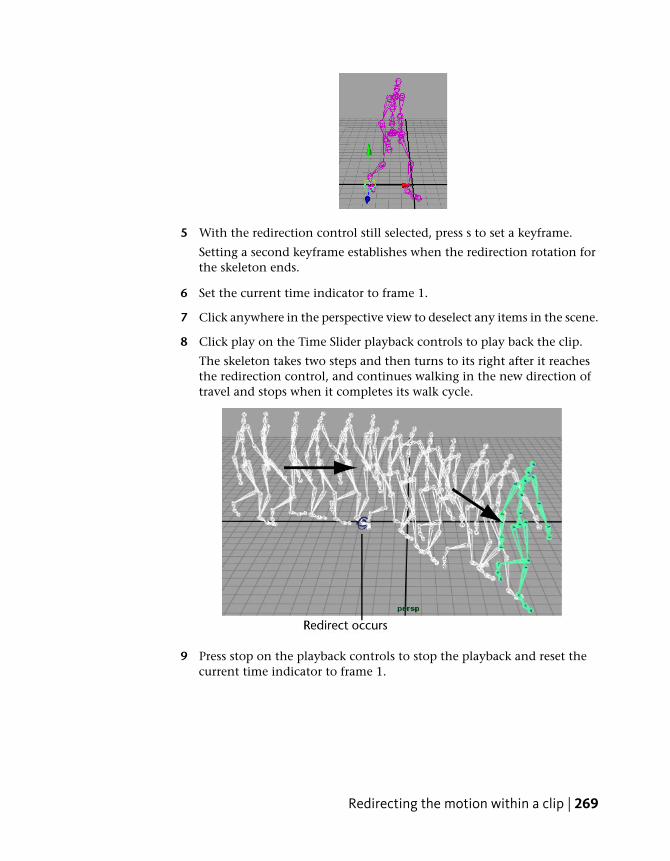
5 With the redirection control still selected, press s to set a keyframe.
Setting a second keyframe establishes when the redirection rotation forthe skeleton ends.
6 Set the current time indicator to frame 1.
7 Click anywhere in the perspective view to deselect any items in the scene.
8 Click play on the Time Slider playback controls to play back the clip.
The skeleton takes two steps and then turns to its right after it reachesthe redirection control, and continues walking in the new direction oftravel and stops when it completes its walk cycle.
9 Press stop on the playback controls to stop the playback and reset thecurrent time indicator to frame 1.
Redirecting the motion within a clip | 269
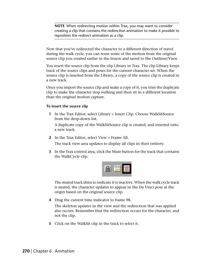
NOTE When redirecting motion within Trax, you may want to considercreating a clip that contains the redirection animation to make it possible toreposition the redirect animation as a clip.
Now that you’ve redirected the character to a different direction of travelduring the walk cycle, you can reuse some of the motion from the originalsource clip you created earlier in the lesson and saved to the Outliner/Visor.
You insert the source clip from the clip Library in Trax. The clip Library keepstrack of the source clips and poses for the current character set. When thesource clip is inserted from the Library, a copy of the source clip is created ina new track.
Once you import the source clip and make a copy of it, you trim the duplicateclip to make the character stop walking and then sit in a different locationthan the original motion capture.
To insert the source clip
1 In the Trax Editor, select Library > Insert Clip. Choose WalkSitSourcefrom the drop-down list.
A duplicate copy of the WalkSitSource clip is created, and inserted ontoa new track.
2 In the Trax Editor, select View > Frame All.
The track view area updates to display all clips in their entirety.
3 In the Trax control area, click the Mute button for the track that containsthe WalkCycle clip.
The muted track dims to indicate it is inactive. When the walk cycle trackis muted, the character updates to appear in the Da Vinci pose at theorigin based on the original source clip.
4 Drag the current time indicator to frame 98.
The skeleton updates in the view and the redirection that was appliedalso occurs. Remember that the redirection occurs for the character, andnot the clip.
5 Click on the WalkSit clip in the track to select it.
270 | Chapter 6 Animation

6 In the Trax tool bar, click the Trim Clip Before Current Time icon to trimthe section of the clip that occurs before frame 98.
The WalkSit clip is trimmed and the portion of the clip before frame 98is discarded.
7 Click the Mute button again for the track containing the WalkCycle clipto reactivate the track.
The dimmed track becomes active again. The skeleton however hasupdated to an incorrect pose near its previous position. This occursbecause the two active clips overlap, and the character is receivingconflicting positional information as a result. (That is, double translationand rotation information.)
8 Drag the WalkSit clip to the right in its track until its Frame In numbermatches the Frame Out for the WalkCycle clip.
The pose for the skeleton is updated to the correct position.
9 Reset the current time indicator to frame 1.
10 Click play on the Time Slider playback controls to play back theanimation.
The skeleton takes two steps and then turns to its right after it reachesthe redirection control, and continues walking in the new direction oftravel, stops, and then sits.
Redirecting the motion within a clip | 271

11 Press stop on the playback controls to stop the playback and reset thecurrent time indicator to frame 1.
A small jump cut occurs during the transition between the two clips. The jumpcut occurs because the poses for the skeleton do not match from the end ofthe first clip and the beginning of the second. In your own work, try toanticipate how motion will blend between clips when working in Trax. Youcan correct the jump cut in this particular example by extending the WalkCycleclip.
To extend the WalkCycle clip to correct the jump cut
1 In the Trax Editor, double-click on the WalkCycle clip in the C2 region.
The number becomes highlighted indicating you can edit the number.
2 Type 2.2 to edit the clip so it cycles 2.2 times.
The new Frame Out number for the WalkCycle clip becomes 126. It nowoverlaps in time with the WalkSit clip.
3 Drag the WalkSit clip to the right until its Frame In number becomes126.
272 | Chapter 6 Animation

4 Click play on the Time Slider’s playback control to play back theanimation.
The jump cut is less noticeable than before.
5 Press stop on the Time Slider’s playback control.
You have completed this lesson. Before leaving this lesson, reset the jointsize back to its default setting.
To reset the joint size
1 From the main menu, select Display > Animation.
The Joint Display Scale window appears.
2 Set the Joint Display Scale to 1.
3 Close the Joint Display Scale window.
Beyond the lessonIn this lesson, you learned some fundamental techniques for using thenonlinear animation tools in Trax. You learned how to:
■ Key animation sequences for use as nonlinear clips in Trax.Clips can contain minimal or many animated attributes. You can createclips from existing animation or key animation specifically for use in clips.You should consider what attributes you need represented in a clip whenyou key the animation before you decide to use nonlinear animation inyour work. In this way, a clip can be used to control a specific attribute.
■ Create clips from your animation sequences for use in the Trax Editor.
Beyond the lesson | 273

When you create a clip, a character set is created if one does not alreadyexist. You can load and work with multiple character sets in the Trax Editor.To select different character sets when working in Trax you can use theSelect Current Character drop-down menu. Clips can also be arranged,scaled, and moved as groups. For more information see Move clips andTrack view area in the Maya Help.
■ Use the Trax editor to position, re-arrange, cycle, and scale clips in orderto create and modify animation sequences in the scene.If a character animates or scales in a manner you had not expected whenworking in Trax, you may want to check to see if the clips overlap or arearranged in a manner that doesn’t provide the expected results. In addition,a clip containing motion that is intended to be appended to another clip’smotion must have its Offset attribute set to Relative, and Absolute Rotationsset to On (in most instances). There are many other tasks you can performwith clips in the Trax Editor that are beyond the scope of this lesson. Formore information see Nonlinear animation components in Trax in theMaya Help.
■ Use the Trax Editor to work with motion capture data.The Trax Editor is useful when working with motion capture data. Sincemotion capture data usually contains a lot of keyframe information, theTrax Editor can be useful for creating, modify, and extending the motiondata provided. Cycling and redirecting motion are two methods that canbe used to get more from your motion capture data. For more informationsee the section on Motion Capture Animation in the Maya Help.
■ Redirect the motion for a character using the Redirect tool.You can use redirection controls to redirect any type of motion in Maya(Keyframe, motion capture, expressions, dynamics, and so on). For moreinformation and additional examples on redirection see Redirect the motionof an animated character in the Maya Help.
■ Trim clips in the Trax Editor.You can trim a clip either before or after the current time indicatordiscarding the remainder of the clip in the process. You can also split aclip into two parts. The original source clip is not affected. For moreinformation see Split clips in the Maya Help.
Blending clips
You can blend the animation between clips. Blends allow you to create smoothtransitions and mixes between different motions. A blend can be appliedbetween any two clips that overlap entirely, partially, or not at all. The bestresults are obtained when blending between similar motions. In some
274 | Chapter 6 Animation
situations, a blend can be used to correct jump cuts. For more informationsee Create and edit blends in the Maya Help.
Key into clip
You can set keyframes to alter the animation within a clip. This process iscalled Keying into a clip. When you key into a clip, keyframes are placed atthe current time on all the animation curves in the selected clip. For moreinformation see Key into a clip in the Maya Help.
Time Warps
Time Warps let you change the timing of a clip without modifying the clip'sanimation curves. You modify the Time Warp by editing the animation curvethat controls the warp. Time Warps can also be used to reverse the animationin a clip. For more information see Create and edit time warps in the MayaHelp.
Visor and Outliner
Both the Visor and Outliner can be used to access clips. The Visor provides agraphical interface to access other resources (such as clips, poses, shaders,textures, and brushes) in your scene. The Outliner displays clips in a textualmanner, and is a bit more compact.
Audio clips
You can display and play multiple audio files in Trax allowing you tosynchronize your motion clips to specific audio events (sound effects, musicalnotes, drum beats) in the audio file. Once you import an audio file into Trax,you can then move and rename the audio clip. For more information seeWork with audio in the Maya Help.
Beyond the lesson | 275

Lesson 5: Inverse kinematics
Introduction
Inverse Kinematics (IK) allows you to efficiently pose your models andcharacters for animation. You pose the skeleton by positioning IK handles,usually located at the end of an IK joint chain (for example at the hand). Therotations for the other joints are calculated automatically by an IK solver. AnIK solver calculates the rotations of each joint back up the hierarchy of thejoint chain based on the position of the IK handle. See Creating a skeletonhierarchy on page 281 for more information on skeletons and joints.
By contrast, Forward Kinematics (FK) requires you to rotate each joint in turnuntil you have the desired pose for a keyframe. This can be a tedious processwhen posing a complex skeleton. When using Inverse Kinematics, it’s fasterto pose a character because the joint rotations further up the hierarchy arecalculated automatically based on the placement of the IK Handle. Using bothFK and IK techniques on the same skeleton is called FK/IK blending.
IK is obviously useful for posing animated characters that have a skeleton andhas other applications, such as posing skeletons within mechanical-like models.
The goal of this lesson is to animate a mechanical arm so that it extends intoa position over a cargo box, picks up and moves the cargo box to anotherlocation, and then sets it down.
As you work through the lesson, you’ll learn about many of the basic featuresrelated to skeleton hierarchies, IK, and parent constraints. Some initial setup
276 | Chapter 6 Animation
of the model and IK is required so that it can be posed and keyframed toprovide a convincing animation.
In this lesson you learn how to:
■ Create and use hierarchies to define logical relationships betweenanimatable objects.
■ Combine the components of a 3D mechanical arm model into ahierarchical grouping.
■ Construct a skeleton for use with IK.
■ Combine the skeleton with the mechanical arm model by parenting thecomponents into a hierarchy.
■ Create an IK system to allow the skeleton hierarchy to be posed.
■ Create a control object to manipulate the IK system.
■ Use constraints to control the position and orientation of componentswithin the IK system.
■ Limit the range of movement on the IK system.
■ Pose and set keyframes for the IK system.
■ Animate an object by constraining its motion to two or more objects.
Open the scene for the lessonIn this lesson, you work with a scene we created for your use. In the first stepsof this lesson, you open the scene and view the various elements that havebeen created for your use.
1 Make sure you’ve done the steps in Preparing for the lessons on page 199.
2 Open the scene file named IK_MechArm.mb.
This file can be found in the GettingStarted directory that you set asyour Maya project: GettingStarted/Anim.
The scene contains a model of a mechanical arm and a cargo box to bemoved by the arm. The components of the mechanical arm include:
■ A cargo magnet cup on the end
■ Three arm segments
Open the scene for the lesson | 277

■ A base for the arm to swivel about
■ A four-legged base for the assembly
To work with this model using IK you must create a hierarchy for it.
Understanding hierarchiesInverse Kinematics relies on hierarchical relationships between the componentsof a model and the IK system to pose and animate the components. Beforeusing Inverse Kinematics it is important to understand hierarchies in Maya.
A hierarchy is composed of a series of nodes that are combined for somepurposeful relationship. Individual nodes may represent the surfaces of amodel, a network of textures that describe a shading material, or series ofjoints in a skeleton. Hierarchies are structured in a top-down manner, withone node at the top (the parent node or root node) and other nodes (child nodesor leaf nodes) attached and interconnected beneath the top node.
Selecting the parent node at the top of the hierarchy also selects the itemscontained in the hierarchy below. Selecting a child node lower in the hierarchyselects any child nodes that are lower in the hierarchy.
Hierarchies allow you to create complex structures with relationships betweencomponents. For example, when you animate a hierarchical model, you simply
278 | Chapter 6 Animation

need to select and move the parent node of the hierarchy and the rest of themodel (child nodes) also moves.
Regardless of whether you decide to animate the mechanical arm using FK orIK, or a combination of both methods on the same model, the best approachinvolves making the mechanical arm model into a hierarchical structure.
Creating a hierarchy for the mechanical arm ensures that:
■ Components of the hierarchy can be rotated as if they were one unit. Acommon pivot point is created at the parent node level. This allows theseparate components to rotate as one unit based on their membership inthe hierarchy. For example, if the mechanical arm’s base (parent node) isrotated, anything lower down the hierarchy, for example, the mechanicalarm which is constructed of child nodes, will also rotate because of itsmembership and position in the hierarchy.
■ When a particular segment of the model is posed and keyframed, thecomponents that are lower in the hierarchy are also posed and keyframed.
Viewing hierarchies using the HypergraphIn the following steps, you use the Hypergraph to view the hierarchy for themechanical arm. The Hypergraph is a scene management editor that presentsa graphical view of the scene hierarchy. It allows you to more easily create,understand, and manage the hierarchy of objects and nodes in your scene.
To view hierarchies using the Hypergraph
1 From the perspective view’s panel menu, select Panels > Layouts > TwoPanes Stacked.
The workspace displays two panels stacked on top of each other with anidentical perspective view of the scene.
2 In the lower panel, select Panels > Hypergraph Panel > HypergraphHierarchy.
The lower panel displays the Hypergraph.
Viewing hierarchies using the Hypergraph | 279
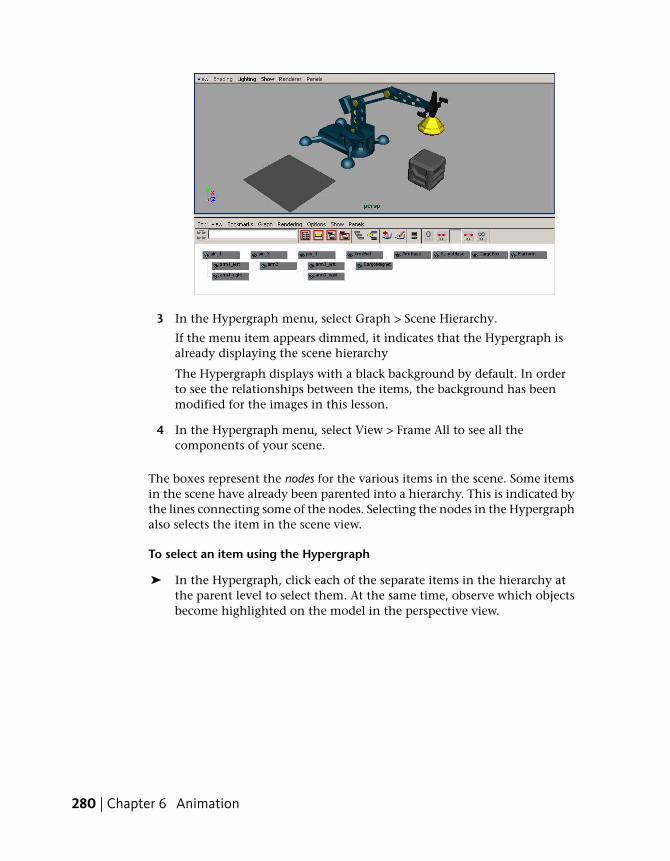
3 In the Hypergraph menu, select Graph > Scene Hierarchy.
If the menu item appears dimmed, it indicates that the Hypergraph isalready displaying the scene hierarchy
The Hypergraph displays with a black background by default. In orderto see the relationships between the items, the background has beenmodified for the images in this lesson.
4 In the Hypergraph menu, select View > Frame All to see all thecomponents of your scene.
The boxes represent the nodes for the various items in the scene. Some itemsin the scene have already been parented into a hierarchy. This is indicated bythe lines connecting some of the nodes. Selecting the nodes in the Hypergraphalso selects the item in the scene view.
To select an item using the Hypergraph
➤ In the Hypergraph, click each of the separate items in the hierarchy atthe parent level to select them. At the same time, observe which objectsbecome highlighted on the model in the perspective view.
280 | Chapter 6 Animation
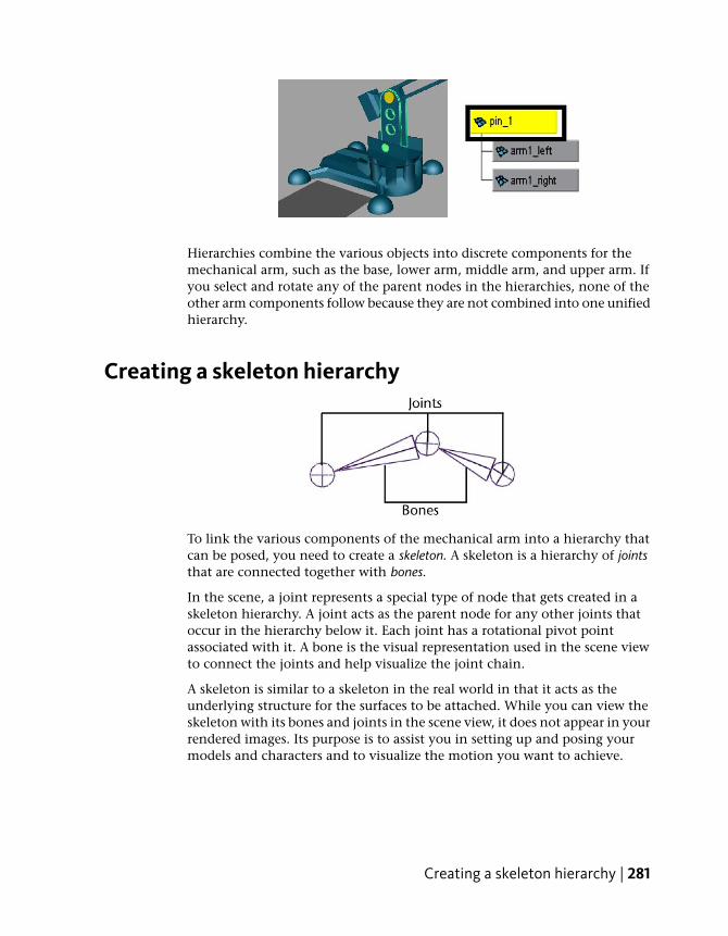
Hierarchies combine the various objects into discrete components for themechanical arm, such as the base, lower arm, middle arm, and upper arm. Ifyou select and rotate any of the parent nodes in the hierarchies, none of theother arm components follow because they are not combined into one unifiedhierarchy.
Creating a skeleton hierarchy
To link the various components of the mechanical arm into a hierarchy thatcan be posed, you need to create a skeleton. A skeleton is a hierarchy of jointsthat are connected together with bones.
In the scene, a joint represents a special type of node that gets created in askeleton hierarchy. A joint acts as the parent node for any other joints thatoccur in the hierarchy below it. Each joint has a rotational pivot pointassociated with it. A bone is the visual representation used in the scene viewto connect the joints and help visualize the joint chain.
A skeleton is similar to a skeleton in the real world in that it acts as theunderlying structure for the surfaces to be attached. While you can view theskeleton with its bones and joints in the scene view, it does not appear in yourrendered images. Its purpose is to assist you in setting up and posing yourmodels and characters and to visualize the motion you want to achieve.
Creating a skeleton hierarchy | 281

Skeletons are integral to the animation of any character or hierarchical model.Examples of characters that use skeletons are two and four legged animals.Skeletons are also useful for animating other organic components such as thetail of an animal, a tentacle of an octopus, or a snake.
In the following steps, you create a simple skeleton consisting of four jointsthat you combine with the mechanical arm model into a skeleton hierarchy,allowing you to pose and animate the model.
To create a skeleton for the mechanical arm
1 In the perspective view menu, select Panels > Orthographic > side.
The view updates to display the side view.
You need to view the components of the mechanical arm fully in theside view so you can draw the joints for the skeleton.
2 Resize the side view to a larger size by dragging the border between theside and Hypergraph panel views downwards.
3 In the side view menu, select Shading > Wireframe (Hotkey 4).
282 | Chapter 6 Animation
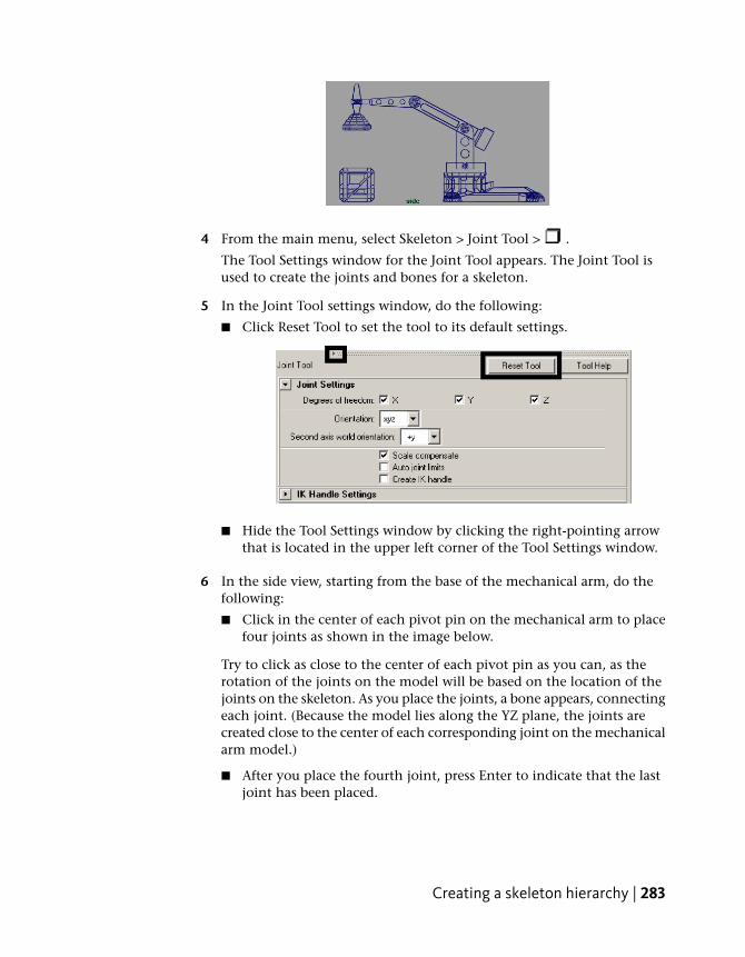
4 From the main menu, select Skeleton > Joint Tool > .
The Tool Settings window for the Joint Tool appears. The Joint Tool isused to create the joints and bones for a skeleton.
5 In the Joint Tool settings window, do the following:
■ Click Reset Tool to set the tool to its default settings.
■ Hide the Tool Settings window by clicking the right-pointing arrowthat is located in the upper left corner of the Tool Settings window.
6 In the side view, starting from the base of the mechanical arm, do thefollowing:
■ Click in the center of each pivot pin on the mechanical arm to placefour joints as shown in the image below.
Try to click as close to the center of each pivot pin as you can, as therotation of the joints on the model will be based on the location of thejoints on the skeleton. As you place the joints, a bone appears, connectingeach joint. (Because the model lies along the YZ plane, the joints arecreated close to the center of each corresponding joint on the mechanicalarm model.)
■ After you place the fourth joint, press Enter to indicate that the lastjoint has been placed.
Creating a skeleton hierarchy | 283

7 In the Hypergraph, dolly the view to see the skeleton node hierarchy youjust created. (It appears at the right side of the view.)
8 In the Hypergraph, select the joint1 node.
The entire skeleton becomes selected. Any rotations on this node alsoaffect anything lower down the hierarchy.
9 Select joint2 (You can also press the down arrow on your keyboard toselect further down the hierarchy).
The skeleton is selected from joint2 downwards in the hierarchy. Anyrotations that you make on this node affect only joint2 and nodes belowjoint2.
284 | Chapter 6 Animation

Once a skeletal hierarchy is created, the various surface components can beadded to the hierarchy.
Parenting a model into a skeleton hierarchyParenting is the term used when placing a node beneath another in a hierarchyso it becomes the child of the node above it (its parent) in the hierarchy.
In the following steps, you add the surfaces of the mechanical arm model intothe skeleton hierarchy. This process links the models’ surfaces to the skeletonhierarchy making it possible to pose and animate the model like a realmechanical arm. Using the Hypergraph to select the nodes allows you to bettervisualize the process and the hierarchical relationships that result.
NOTE The following parenting procedure works well for the mechanical arm (noorganic bending or deformation occurs) and provides one technique for addingmodeled objects to a skeletal hierarchy.
A more common technique for combining a character model into a skeletonhierarchy is referred to as skinning or binding. The Bind Skin tool combines thesurface components and joints together into a hierarchy and also takes into accountany deformations that may occur when a character bends or flexes (such as at theknees, waist, neck, or elbows). Maya provides a few methods for skinning. Formore information see Skeletons and skinning in the Maya Help. For a tutorial onskinning see the Smooth Skinning lesson in the Character Setup chapter in thisguide.
To parent the mechanical arm into the skeleton
1 In the Hypergraph menu, select View > Frame All.
The Hypergraph displays all the nodes for the scene.
2 In the Hypergraph, select the node named ArmEnd and then shift-selectthe node named joint4.
The order of selection is important. You want to select the child nodefirst, and then shift-select the item that will become the parent nodesecond.
3 In the main menu, select Edit > Parent (Hotkey p).
In the Hypergraph, joint4 is now the parent node for the Arm_end nodein the skeleton hierarchy.
Parenting a model into a skeleton hierarchy | 285
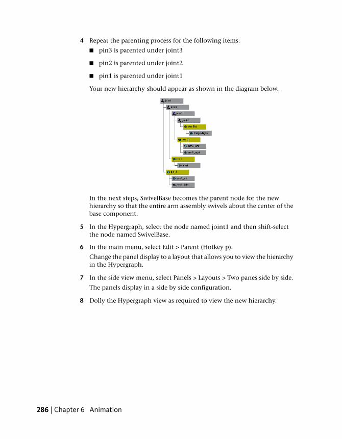
4 Repeat the parenting process for the following items:
■ pin3 is parented under joint3
■ pin2 is parented under joint2
■ pin1 is parented under joint1
Your new hierarchy should appear as shown in the diagram below.
In the next steps, SwivelBase becomes the parent node for the newhierarchy so that the entire arm assembly swivels about the center of thebase component.
5 In the Hypergraph, select the node named joint1 and then shift-selectthe node named SwivelBase.
6 In the main menu, select Edit > Parent (Hotkey p).
Change the panel display to a layout that allows you to view the hierarchyin the Hypergraph.
7 In the side view menu, select Panels > Layouts > Two panes side by side.
The panels display in a side by side configuration.
8 Dolly the Hypergraph view as required to view the new hierarchy.
286 | Chapter 6 Animation
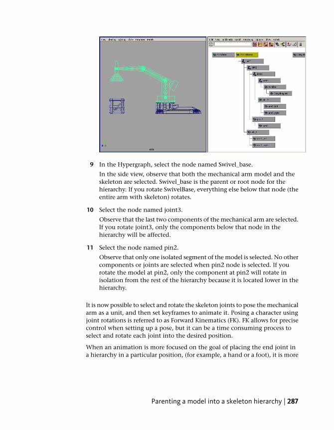
9 In the Hypergraph, select the node named Swivel_base.
In the side view, observe that both the mechanical arm model and theskeleton are selected. Swivel_base is the parent or root node for thehierarchy. If you rotate SwivelBase, everything else below that node (theentire arm with skeleton) rotates.
10 Select the node named joint3.
Observe that the last two components of the mechanical arm are selected.If you rotate joint3, only the components below that node in thehierarchy will be affected.
11 Select the node named pin2.
Observe that only one isolated segment of the model is selected. No othercomponents or joints are selected when pin2 node is selected. If yourotate the model at pin2, only the component at pin2 will rotate inisolation from the rest of the hierarchy because it is located lower in thehierarchy.
It is now possible to select and rotate the skeleton joints to pose the mechanicalarm as a unit, and then set keyframes to animate it. Posing a character usingjoint rotations is referred to as Forward Kinematics (FK). FK allows for precisecontrol when setting up a pose, but it can be a time consuming process toselect and rotate each joint into the desired position.
When an animation is more focused on the goal of placing the end joint ina hierarchy in a particular position, (for example, a hand or a foot), it is more
Parenting a model into a skeleton hierarchy | 287

efficient to use Inverse Kinematics to pose the skeleton. For more informationon forward and inverse kinematics, see Posing skeletons in the Maya Help.
NOTE It’s not a simple matter to state that one technique or another is the onlyapproach to achieving a desired result when animating in Maya. You must decidewhether a particular technique works for a particular scenario based on the optionsit provides. A combination of animation techniques can be creatively used in avariety of ways.
Applying IK to a skeleton hierarchyIK allows you to control the joint rotations in a skeleton using an IK handle.You pose the skeleton by positioning the IK handle (usually located at theend extremity of the skeleton) and having the rotations for the other jointscalculated automatically by the IK solver. In the steps that follow, you applyIK to the skeletal hierarchy.
To create an IK handle for the mechanical arm
1 From the main menu, select Skeleton > IK Handle Tool > .
The IK Handle Tool Settings window for the Joint Tool appears. Whenthe mouse pointer is in the orthographic view its appearance changes tothe tool's cross hair cursor.
2 In the IK Handle Tool Settings window, do the following:
■ Click Reset Tool to set the tool to its default settings.
■ Set the IK Handle Settings: Current Solver - ikSCsolver.
288 | Chapter 6 Animation

■ Hide the Tool Settings window by clicking the right-pointing arrowthat is located in the upper left corner of the Tool Settings window.
The ikSCsolver setting selects the IK Single Chain Solver. This solverensures that the joints in the skeleton will lie along a single plane. Thissolver is well suited for the mechanical arm, because the arm doesn’tneed to twist, unlike a real arm.
3 Working in the side view, starting from the base of the mechanical arm,do the following:
■ Click on the skeleton joint at the base of the mechanical arm.
■ Click on the skeleton joint at the tip of the mechanical arm. (The IKTool is designed to attach to the joints closest to your selection point.)
In the side view, the IK handle is drawn as a line from the start and endjoints of the IK chain.
4 In the Hypergraph menu, select View > Frame All.
In the Hypergraph, two new nodes appear in the hierarchy that representthe IK chain: an IK Handle node and an end effector node.
Applying IK to a skeleton hierarchy | 289

5 In the Hypergraph, select the node named ikHandle1.
The IK Handle (in combination with the end effector) is used by the IKsolver to calculate the rotation of the joints in the IK chain. By default,the IK Handle is located at the last joint of the IK chain in the scene view.
6 Select the Move Tool from the Toolbox, and drag the Move Tool’s Z axismanipulator (blue arrow) to reposition the mechanical arm.
When you drag the manipulator, the skeleton and mechanical arm modelare repositioned.
7 Reset the mechanical arm to its previous position by selecting Edit >Undo, Redo, Repeat until the mechanical arm is positioned into itsprevious orientation.
NOTE When using the Undo feature, do not undo so many times youinadvertently undo the IK handle you’ve just created.
The next steps describe how to manipulate the IK Handle using a controlobject.
Creating a control object for an IK systemUsing the IK Handle to pose an IK chain is generally not a good practice. TheIK Handle can be challenging to select in the scene view, especially when it’sgrouped into a hierarchy that includes a skeleton and other surfacecomponents. A better practice is to create a control object.
290 | Chapter 6 Animation
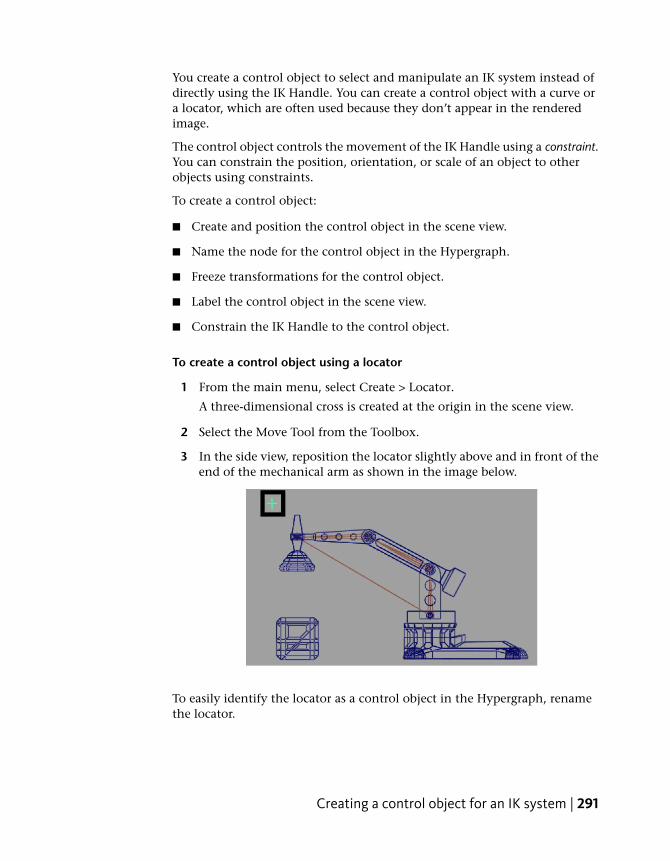
You create a control object to select and manipulate an IK system instead ofdirectly using the IK Handle. You can create a control object with a curve ora locator, which are often used because they don’t appear in the renderedimage.
The control object controls the movement of the IK Handle using a constraint.You can constrain the position, orientation, or scale of an object to otherobjects using constraints.
To create a control object:
■ Create and position the control object in the scene view.
■ Name the node for the control object in the Hypergraph.
■ Freeze transformations for the control object.
■ Label the control object in the scene view.
■ Constrain the IK Handle to the control object.
To create a control object using a locator
1 From the main menu, select Create > Locator.
A three-dimensional cross is created at the origin in the scene view.
2 Select the Move Tool from the Toolbox.
3 In the side view, reposition the locator slightly above and in front of theend of the mechanical arm as shown in the image below.
To easily identify the locator as a control object in the Hypergraph, renamethe locator.
Creating a control object for an IK system | 291

To rename the control object using the Hypergraph
1 In the Hypergraph, right-click the node named locator1. Choose Renamefrom the pop-up menu that appears.
The locator1 name is highlighted on the node.
2 Type the name ArmControl and press Enter to save the name for thelocator.
Before you constrain the IK handle to the control object, you need to freezethe transformations for the control object. Freeze Transformations zeros thetransformations for an object without changing the position of the object.This is another good practice; If it becomes necessary to reset the arm to itsdefault position, you can set the transformation on the control object to zero,and the arm will return to this default pose.
To freeze the transformations for the control object
1 In the Hypergraph, select the node named ArmControl.
The control object is selected in the scene view.
2 In the main menu, select Modify > Reset Transformations, Freeze
Transformations > .
3 In the Freeze Transformation Options window do the following:
■ Select Edit > Reset Settings to set the tool to its default settings.
■ Click the Freeze Transform button.
The transformations for ArmControl are set to zero. From this pointonwards, you can reset its position to this location by zeroing itstranslations in the Channel Box.
292 | Chapter 6 Animation
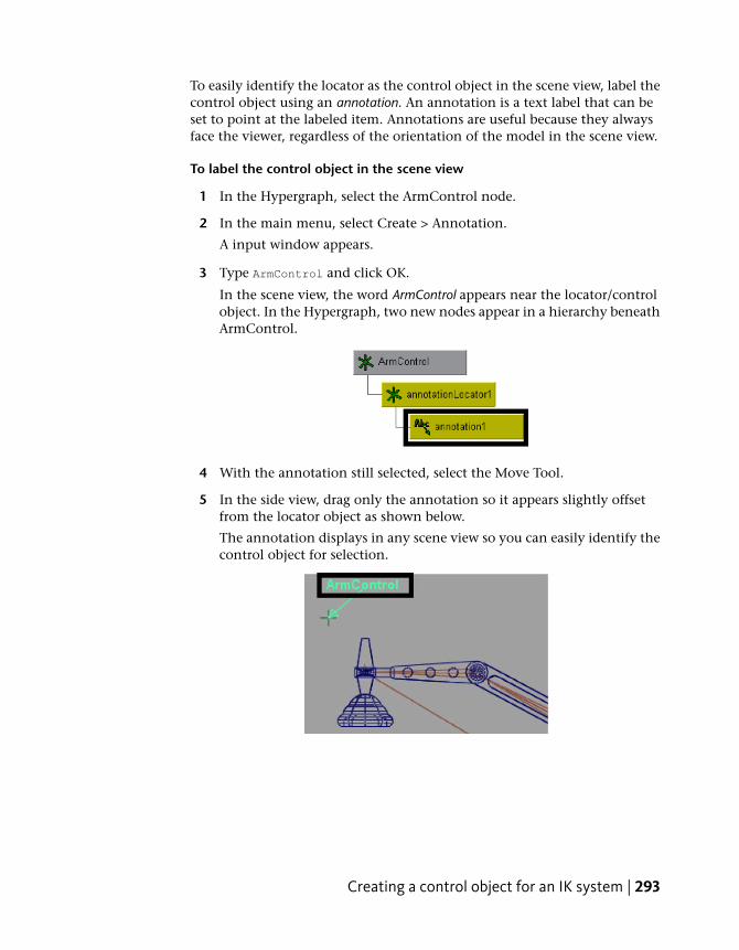
To easily identify the locator as the control object in the scene view, label thecontrol object using an annotation. An annotation is a text label that can beset to point at the labeled item. Annotations are useful because they alwaysface the viewer, regardless of the orientation of the model in the scene view.
To label the control object in the scene view
1 In the Hypergraph, select the ArmControl node.
2 In the main menu, select Create > Annotation.
A input window appears.
3 Type ArmControl and click OK.
In the scene view, the word ArmControl appears near the locator/controlobject. In the Hypergraph, two new nodes appear in a hierarchy beneathArmControl.
4 With the annotation still selected, select the Move Tool.
5 In the side view, drag only the annotation so it appears slightly offsetfrom the locator object as shown below.
The annotation displays in any scene view so you can easily identify thecontrol object for selection.
Creating a control object for an IK system | 293

To simplify the display of the Arm Control node
➤ In the Hypergraph, right-click the ArmControl node. Choose Collapsefrom the pop-up menu. (You can also double-click a node to collapse orexpand the hierarchy below it.)
The ArmControl node appears as a single node instead of the previousthree node hierarchy. The small arrowhead on the lower left-hand cornerof the node indicates that the node is collapsed.
The control object must be linked to the IK Handle to control the IK Handle.
Constraining an IK systemYou can constrain the IK Handle to the control object (ArmControl) using apoint constraint. A point constraint allows the transformation attributes of oneobject to be controlled by the transformations of another object. For example,you select and position ArmControl without having to touch the IK Handle.You also set the constraint so ArmControl maintains the current distance(offset) from the IK Handle. The offset ensures that the constrained IK handledoesn’t move to the same position as the control object.
To constrain the IK Handle to the control object
1 In the Hypergraph, select the ArmControl node and then shift select theikHandle1 node.
The order of selection when applying a constraint is important: you mustselect the constraining object first, and the item to be constrained second.
2 In the main menu, select Constrain > Point > .
The Point Constraint Options window appears.
3 In the Point Constraint Options window, do the following:
■ Select Edit > Reset Settings to set the tool to its default settings.
■ Turn on the Maintain Offset setting.
■ Click the Add button.
294 | Chapter 6 Animation

The IK handle is constrained to the control object. In the Hypergraph, aconstraint node is created beneath the ikHandle1 node.
4 In the Hypergraph, select only the ArmControl node.
5 In the Toolbox, select the Move Tool.
6 In the side view, drag the manipulator to reposition the control object.(Experiment with a few different positions in the side view only.)
When you drag the manipulator, the control object moves, which in turnmoves the IKHandle. Because the IK handle controls the skeleton andthe mechanical arm model, they also move. The offset between the controlobject and the IK Handle is maintained.
The Cargo Magnet does not continuously point downwards when rotated. Itsorientation is based on the rotation it had in its original position.
The mechanical arm will be easier to pose if you set Cargo Magnet to beoriented downwards towards the floor of the scene regardless of the orientationof the other components of the arm.
Constraining an IK system | 295

You make CargoMagnet point downwards using an orient constraint. An orientconstraint constrains the orientation (rotation) of the X, Y, and Z axes of oneobject to match those of the constraining (target) object.
In the next steps, you reset the position of the mechanical arm to its defaultposition, and then apply an orient constraint to the last joint in the IK systemso that its orientation matches the control object. The effect is thatCargoMagnet points downwards regardless of any other movement in thescene.
To set the IK system to its default position
1 In the Hypergraph, select the ArmControl node.
2 Open the Channel Box by clicking the Show/Hide Channel Box icon.
3 In the Channel Box, set the X, Y, and Z transformations for ArmControlto 0.
Zeroing the transformations on ArmControl resets the mechanical armto its home position because of the freeze transformations step youperformed in the previous section.
4 Close the Channel Box by clicking the Show/Hide Channel Box icon.
To apply an orient constraint for the IK system
1 In the Hypergraph menu, select View > Frame All.
The Hypergraph displays all the nodes in the scene.
296 | Chapter 6 Animation
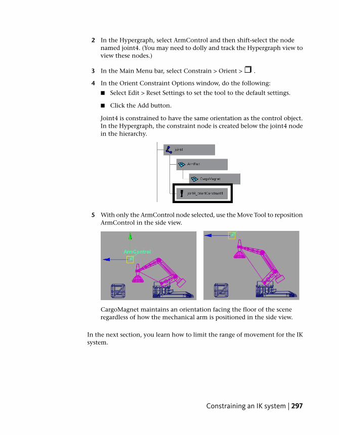
2 In the Hypergraph, select ArmControl and then shift-select the nodenamed joint4. (You may need to dolly and track the Hypergraph view toview these nodes.)
3 In the Main Menu bar, select Constrain > Orient > .
4 In the Orient Constraint Options window, do the following:
■ Select Edit > Reset Settings to set the tool to the default settings.
■ Click the Add button.
Joint4 is constrained to have the same orientation as the control object.In the Hypergraph, the constraint node is created below the joint4 nodein the hierarchy.
5 With only the ArmControl node selected, use the Move Tool to repositionArmControl in the side view.
CargoMagnet maintains an orientation facing the floor of the sceneregardless of how the mechanical arm is positioned in the side view.
In the next section, you learn how to limit the range of movement for the IKsystem.
Constraining an IK system | 297

Limiting the range of motion of an IK systemIt’s possible to move ArmControl so that the mechanical arm fully extendsto a straight position or orients itself to other positions that you don’tnecessarily want.
You can limit the range of motion of the arm to ensure that the IK systemposes in a predictable manner. In the following section, you limit the motionfor the IK system as follows:
■ Lock the translation of the control object (ArmControl) so that it can onlymove in Y and Z. By locking the X channel so it cannot be selected ormodified, the arm will not be able to move from side to side.
■ Lock the rotations on the swiveling base for the arm so it only rotatesabout its Y axis, and not about its X or Z axes.
■ Limit the translations for the Arm Control so the mechanical arm cannotfully extend to a straightened position.
To lock the Translate X channel for ArmControl
1 In the Hypergraph, select the ArmControl node.
2 Open the Channel Box to view the transform channels for ArmControl.
3 Set all Translate or Rotate channels to 0, if they are not already.
4 In the Channel Box, select the Translate X channel by clicking on itsname.
5 Right click on the word Translate X.
A drop-down menu appears.
6 From the drop-down menu, choose Lock Selected.
298 | Chapter 6 Animation

The numerical field for Translate X is dimmed indicating that the channelis locked. If you try to move ArmControl in X, it will not be possibleunless you unlock the Translate X channel.
To lock the Rotate X and Z channels for SwivelBase
1 In the Hypergraph, select only the SwivelBase node.
2 Open the Channel Box to view the rotation channels for SwivelBase.
3 Set all Translate or Rotate channels to 0, if they are not already.
4 In the Channel Box, select the Rotate X and Rotate Z channels bycontrol-clicking on their names.
5 Right click on either of the selected names.
A drop-down menu appears.
6 From the drop-down menu, select Lock Selected.
To confirm that the Rotate X & Z channels are locked
1 In the Hypergraph, ensure only the SwivelBase node is selected.
2 In the view, select Panels > Orthographic > top.
3 In the view, select Shading > Smooth Shade All.
4 Dolly the top view so you can fully view the mechanical arm as shownbelow.
5 Using the Channel Box, rotate SwivelBase by typing 45 in the Rotate Ychannel and pressing Enter.
Limiting the range of motion of an IK system | 299

SwivelBase rotates in the view but the mechanical arm does not rotate.You first might think something is wrong because SwivelBase and all ofthe arm’s skeletons and surfaces are parented into the same hierarchy.
NOTE You may sometimes discover that something doesn’t work in themanner you originally anticipated when setting up an IK system. When thisoccurs, it’s useful to stop and diagnose why something is working the wayit is (or not working the way it should). In that way you can retrace youractions to determine where the problem resides.
ArmControl and IK Handle are not parented into the SwivelBase hierarchy.Because ArmControl and IK Handle control the movements of the mechanicalarm, they must be parented into the SwivelBase hierarchy in order for the armto rotate when SwivelBase is rotated.
To parent the IK Handle into the skeleton hierarchy
1 In the Hypergraph, select the SwivelBase node.
2 In the Channel Box, reset the Rotate Y channel for SwivelBase to 0.
Setting any previous transformations to zero is necessary before parentingthe IK Handle beneath SwivelBase in the hierarchy.
3 Unselect the SwivelBase node before performing the following steps.
4 In the Hypergraph menu, select View > Frame All.
The Hypergraph displays all the nodes for the scene.
5 In the Hypergraph, shift-select the nodes named ikHandle1, ArmControl,and SwivelBase.
300 | Chapter 6 Animation

The order of selection is important. You want to shift-select the itemsthat will be the child nodes first, and then shift-select the item that willbe the parent node last.
6 In the main menu, select Edit > Parent (Hotkey p).
In the Hypergraph, IKHandle and ArmControl are now child nodes forthe SwivelBase node in the skeleton hierarchy.
7 In the Hypergraph, select only SwivelBase.
8 Using the Channel Box, set Rotate Y for SwivelBase to 45.
When SwivelBase is rotated, the mechanical arm rotates because of itsrelationship within the hierarchy.
9 Reset the Rotate Y value for SwivelBase back to 0.
Finally, you want to limit how far Arm Control can translate away from thebase of the model so the arm does not extend to a fully straightened position.
To determine the settings for the translation limits you need to examine theposition of the mechanical arm in various positions while simultaneouslyviewing the translation values in the Channel Box.
Limiting the range of motion of an IK system | 301
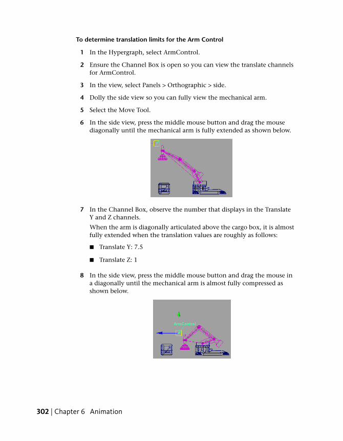
To determine translation limits for the Arm Control
1 In the Hypergraph, select ArmControl.
2 Ensure the Channel Box is open so you can view the translate channelsfor ArmControl.
3 In the view, select Panels > Orthographic > side.
4 Dolly the side view so you can fully view the mechanical arm.
5 Select the Move Tool.
6 In the side view, press the middle mouse button and drag the mousediagonally until the mechanical arm is fully extended as shown below.
7 In the Channel Box, observe the number that displays in the TranslateY and Z channels.
When the arm is diagonally articulated above the cargo box, it is almostfully extended when the translation values are roughly as follows:
■ Translate Y: 7.5
■ Translate Z: 1
8 In the side view, press the middle mouse button and drag the mouse ina diagonally until the mechanical arm is almost fully compressed asshown below.
302 | Chapter 6 Animation
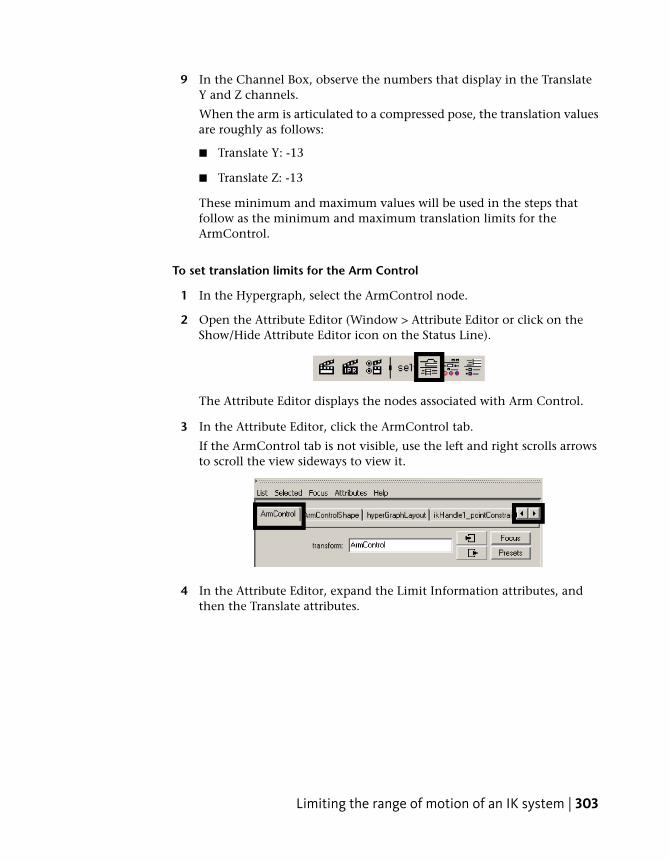
9 In the Channel Box, observe the numbers that display in the TranslateY and Z channels.
When the arm is articulated to a compressed pose, the translation valuesare roughly as follows:
■ Translate Y: -13
■ Translate Z: -13
These minimum and maximum values will be used in the steps thatfollow as the minimum and maximum translation limits for theArmControl.
To set translation limits for the Arm Control
1 In the Hypergraph, select the ArmControl node.
2 Open the Attribute Editor (Window > Attribute Editor or click on theShow/Hide Attribute Editor icon on the Status Line).
The Attribute Editor displays the nodes associated with Arm Control.
3 In the Attribute Editor, click the ArmControl tab.
If the ArmControl tab is not visible, use the left and right scrolls arrowsto scroll the view sideways to view it.
4 In the Attribute Editor, expand the Limit Information attributes, andthen the Translate attributes.
Limiting the range of motion of an IK system | 303
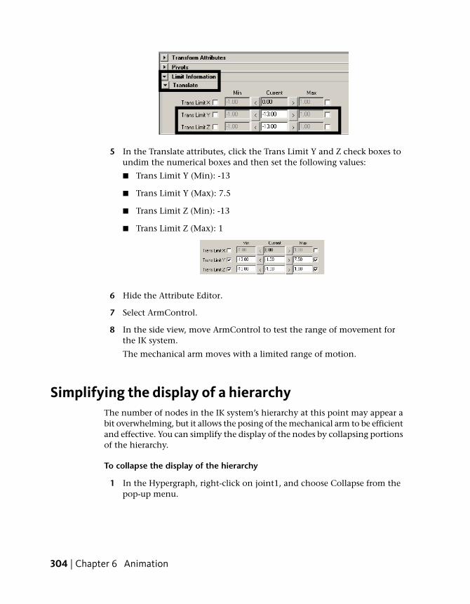
5 In the Translate attributes, click the Trans Limit Y and Z check boxes toundim the numerical boxes and then set the following values:
■ Trans Limit Y (Min): -13
■ Trans Limit Y (Max): 7.5
■ Trans Limit Z (Min): -13
■ Trans Limit Z (Max): 1
6 Hide the Attribute Editor.
7 Select ArmControl.
8 In the side view, move ArmControl to test the range of movement forthe IK system.
The mechanical arm moves with a limited range of motion.
Simplifying the display of a hierarchyThe number of nodes in the IK system’s hierarchy at this point may appear abit overwhelming, but it allows the posing of the mechanical arm to be efficientand effective. You can simplify the display of the nodes by collapsing portionsof the hierarchy.
To collapse the display of the hierarchy
1 In the Hypergraph, right-click on joint1, and choose Collapse from thepop-up menu.
304 | Chapter 6 Animation

The child nodes below joint1 disappear, simplifying the display of thehierarchy. The small arrowhead on the corner of the joint1 node indicatesthat a hierarchy exists below joint1. If you later need to view or selectthese nodes you can expand them again.
2 Collapse the ArmControl and IKHandle nodes.
The display of the hierarchy is simplified as shown below.
The IK system is now rigged and ready for animation.
Applying parent constraints on an IK systemTo animate the cargo box so that it is picked up by the mechanical arm youneed a method of constraining the cargo box to the mechanical arm so thatit moves with the arm at specific times in the animation. This is accomplishedusing a parent constraint.
When a parent constraint is applied to an object, the constrained objectbehaves as if it were a child node of the constraining object.
An object can have multiple constraints applied to it. The influence eachconstraint has on the object can be changed by modifying the weight attributefor the parent constraint. The weight attribute is an animatable parameterand can be set to be on or off at specific frames.
In this lesson, the cargo box is constrained to both the ArmControl and thePlatform on the floor. By animating the weight attributes for these two parentconstraints, the cargo box will move from one location to another dependingon which constraint is influencing it at specific times in the animation.
To set up the parent constraints you need to position the constrained objectat the locations where the influence will begin or end, and then set the parentconstraints.
To set parent constraints for the cargo box
1 In the side view menu, select Shading > Smooth Shade All.
2 In the side view menu, select Panels > Perspective > persp.
3 In the Hypergraph, select ArmControl.
Applying parent constraints on an IK system | 305
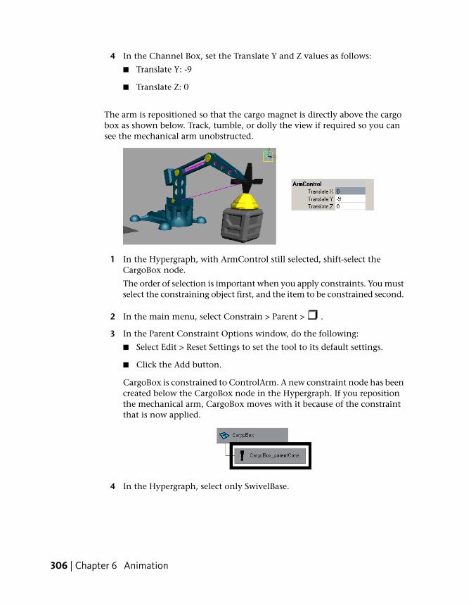
4 In the Channel Box, set the Translate Y and Z values as follows:
■ Translate Y: -9
■ Translate Z: 0
The arm is repositioned so that the cargo magnet is directly above the cargobox as shown below. Track, tumble, or dolly the view if required so you cansee the mechanical arm unobstructed.
1 In the Hypergraph, with ArmControl still selected, shift-select theCargoBox node.
The order of selection is important when you apply constraints. You mustselect the constraining object first, and the item to be constrained second.
2 In the main menu, select Constrain > Parent > .
3 In the Parent Constraint Options window, do the following:
■ Select Edit > Reset Settings to set the tool to its default settings.
■ Click the Add button.
CargoBox is constrained to ControlArm. A new constraint node has beencreated below the CargoBox node in the Hypergraph. If you repositionthe mechanical arm, CargoBox moves with it because of the constraintthat is now applied.
4 In the Hypergraph, select only SwivelBase.
306 | Chapter 6 Animation

5 In the Channel Box, set the Rotate Y value for SwivelBase as follows:
■ Rotate Y: -100
The mechanical arm and the cargo box are positioned as shown below.
6 In the Hypergraph, select Platform and then shift-select the CargoBoxnode.
7 In the main menu, select Constrain > Parent.
CargoBox is constrained to Platform. This is the second constraint forthe CargoBox.
8 In the Hypergraph, select only CargoBox.
9 In the Channel Box, view the parent constraints for CargoBox.
CargoBox has two parent constraints applied to it: Arm Control andPlatform. In the Channel Box, the numerical settings beside ArmControlW0 and Platform W1 represent the influence weight each parentconstraint has on CargoBox. At this point, each influence weight is set
Applying parent constraints on an IK system | 307
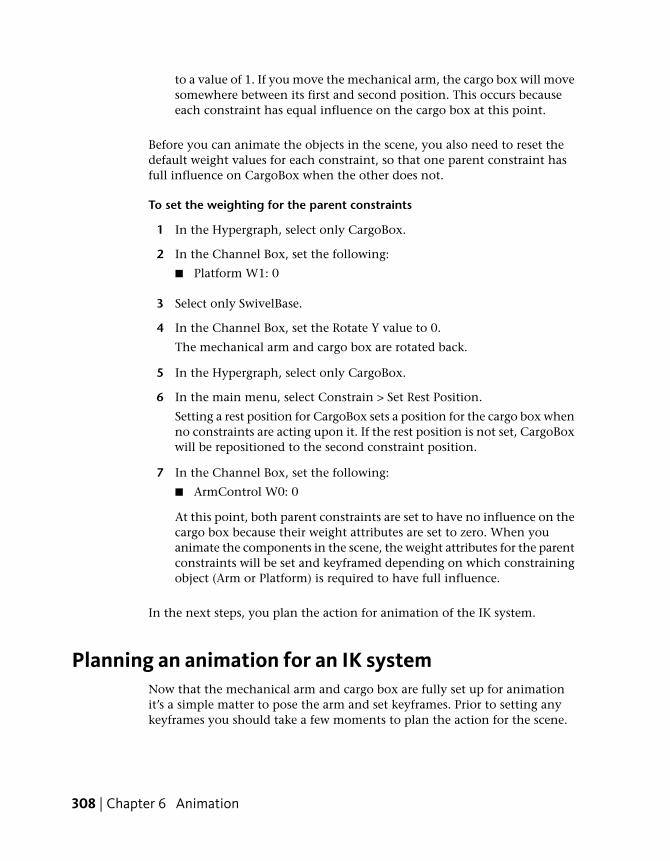
to a value of 1. If you move the mechanical arm, the cargo box will movesomewhere between its first and second position. This occurs becauseeach constraint has equal influence on the cargo box at this point.
Before you can animate the objects in the scene, you also need to reset thedefault weight values for each constraint, so that one parent constraint hasfull influence on CargoBox when the other does not.
To set the weighting for the parent constraints
1 In the Hypergraph, select only CargoBox.
2 In the Channel Box, set the following:
■ Platform W1: 0
3 Select only SwivelBase.
4 In the Channel Box, set the Rotate Y value to 0.
The mechanical arm and cargo box are rotated back.
5 In the Hypergraph, select only CargoBox.
6 In the main menu, select Constrain > Set Rest Position.
Setting a rest position for CargoBox sets a position for the cargo box whenno constraints are acting upon it. If the rest position is not set, CargoBoxwill be repositioned to the second constraint position.
7 In the Channel Box, set the following:
■ ArmControl W0: 0
At this point, both parent constraints are set to have no influence on thecargo box because their weight attributes are set to zero. When youanimate the components in the scene, the weight attributes for the parentconstraints will be set and keyframed depending on which constrainingobject (Arm or Platform) is required to have full influence.
In the next steps, you plan the action for animation of the IK system.
Planning an animation for an IK systemNow that the mechanical arm and cargo box are fully set up for animationit’s a simple matter to pose the arm and set keyframes. Prior to setting anykeyframes you should take a few moments to plan the action for the scene.
308 | Chapter 6 Animation
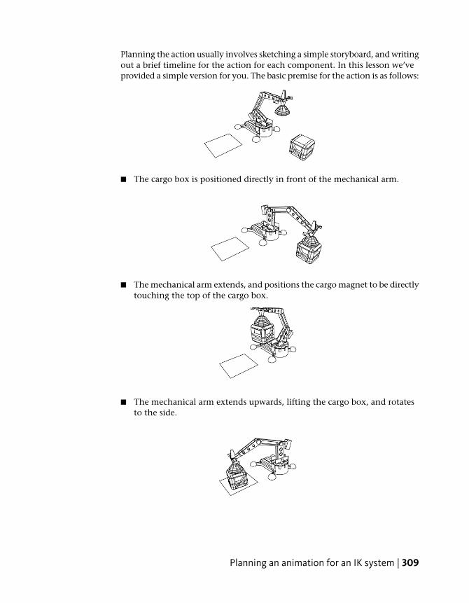
Planning the action usually involves sketching a simple storyboard, and writingout a brief timeline for the action for each component. In this lesson we’veprovided a simple version for you. The basic premise for the action is as follows:
■ The cargo box is positioned directly in front of the mechanical arm.
■ The mechanical arm extends, and positions the cargo magnet to be directlytouching the top of the cargo box.
■ The mechanical arm extends upwards, lifting the cargo box, and rotatesto the side.
Planning an animation for an IK system | 309

■ The mechanical arm lowers the box, placing it in a new position.
■ The mechanical arm extends upwards, leaves the cargo box in the newlocation, and rotates back to its original position.
The table below breaks down the action indicating what action occurs foreach object at the specified keyframes.
Cargo BoxMechanical ArmFrame
Initial positionCollapsed position1
Initial positionVertically extended position30
Initial positionVertically lowered so thatcargo magnet is positionedon top of cargo box
60
Cargo box lifted withmechanical arm
Vertically lifted to extendedposition with cargo box
80
Cargo box repositionedalong with mechanical arm
SwivelBase rotated alongwith arm to side
100
Cargo box is lowered alongwith mechanical arm tosecond position
Vertically lowered alongwith cargo box to secondposition above surface
120
Second positionVertically lifted to extendedposition
140
Second positionSwivelBase rotated witharm to original position
160
Second positionCollapsed position180
310 | Chapter 6 Animation

To pose the mechanical arm you select either the ArmControl or SwivelBasenodes and set a keyframe depending on which component you want to pose:
■ ArmControl controls the movement of the mechanical arm.
■ SwivelBase controls the rotation of the arm.
■ CargoBox’s position is based on the parent constraint weights.
Animating an IK systemThe animation sequence occurs over a 180 frame period. Before you begin toset keyframes you set the playback range in the Animation Timeline/Slider.
To set the playback range in the Time Slider
➤ In the Animation Time and Range Slider, set the following start and endtimes for the animation:
■ Playback Start Time: 1
■ Playback End Time: 180
To simplify the keyframe workflow, you first set keyframes for the mechanicalarm, and then set keyframes for the weight attributes of each parent constraintfor the cargo box.
To set keyframes for the mechanical arm
1 In the Timeline, set the Time Slider to frame 1.
2 Select only ArmControl.
3 In the Channel Box, set the following values:
■ Translate Y: 0
■ Translate Z: -13
4 From the main menu, select Animate > Set Key.
Animating an IK system | 311
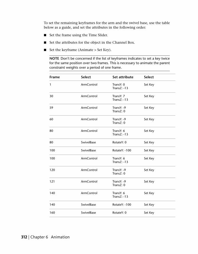
To set the remaining keyframes for the arm and the swivel base, use the tablebelow as a guide, and set the attributes in the following order:
■ Set the frame using the Time Slider.
■ Set the attributes for the object in the Channel Box.
■ Set the keyframe (Animate > Set Key).
NOTE Don’t be concerned if the list of keyframes indicates to set a key twicefor the same position over two frames. This is necessary to animate the parentconstraint weights over a period of one frame.
SelectSet attributeSelectFrame
Set KeyTransY: 0ArmControl1TransZ: -13
Set KeyTransY: 7ArmControl30TransZ: -13
Set KeyTransY: -9ArmControl59TransZ: 0
Set KeyTransY: -9ArmControl60TransZ: 0
Set KeyTransY: 6ArmControl80TransZ: -13
Set KeyRotateY: 0SwivelBase80
Set KeyRotateY: -100SwivelBase100
Set KeyTransY: 6ArmControl100TransZ: -13
Set KeyTransY: -9ArmControl120TransZ: 0
Set KeyTransY: -9ArmControl121TransZ: 0
Set KeyTransY: 6ArmControl140TransZ: -13
Set KeyRotateY: -100SwivelBase140
Set KeyRotateY: 0SwivelBase160
312 | Chapter 6 Animation

SelectSet attributeSelectFrame
Set KeyTransY: 6ArmControl160TransZ: -13
Set KeyTransY: 0ArmControl180TransZ: -13
Once the keyframes for the mechanical arm are set you can use the playbackcontrols to playback the motion for the mechanical arm.
To playback the animation using the playback controls
1 Click play on the TimeSlider playback controls to play the animation.
The mechanical arm animates over 180 frames. The cargo box does notmove because the weight attributes for the parent constraints are set tozero and have not yet been set for the animation.
2 Click stop on the TimeSlider playback controls to stop the playback.
In the next steps, you set keyframes for the parent constraint weight attributesso the cargo box is lifted, moved, and placed in the second location. You setkeys for the weight attributes on the parent constraint node.
To set keyframes for the parent constraint weights
1 In the Timeline, set the Time Slider to frame 1.
2 In the Hypergraph, select the node for the parent constraint directlybelow CargoBox.
3 In the Channel Box, set the following values (if they are not set already):
■ ArmControl W0: 0
■ Platform W1: 0
4 In the Channel Box, select the ArmControl and Platform channels byshift-clicking on the names.
Animating an IK system | 313
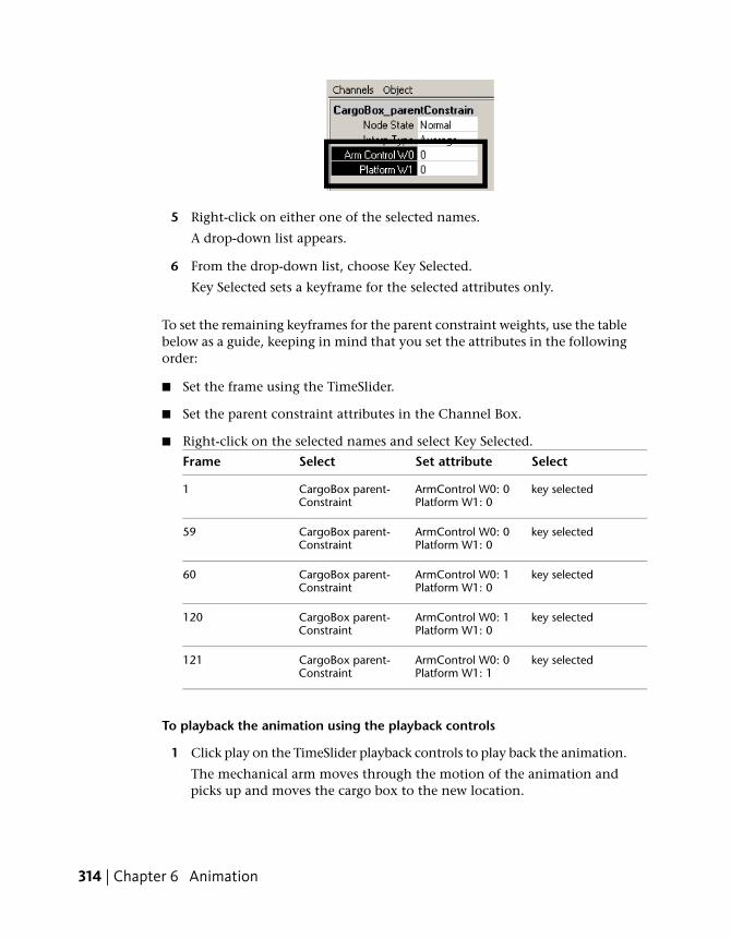
5 Right-click on either one of the selected names.
A drop-down list appears.
6 From the drop-down list, choose Key Selected.
Key Selected sets a keyframe for the selected attributes only.
To set the remaining keyframes for the parent constraint weights, use the tablebelow as a guide, keeping in mind that you set the attributes in the followingorder:
■ Set the frame using the TimeSlider.
■ Set the parent constraint attributes in the Channel Box.
■ Right-click on the selected names and select Key Selected.
SelectSet attributeSelectFrame
key selectedArmControl W0: 0CargoBox parent-Constraint
1Platform W1: 0
key selectedArmControl W0: 0CargoBox parent-Constraint
59Platform W1: 0
key selectedArmControl W0: 1CargoBox parent-Constraint
60Platform W1: 0
key selectedArmControl W0: 1CargoBox parent-Constraint
120Platform W1: 0
key selectedArmControl W0: 0CargoBox parent-Constraint
121Platform W1: 1
To playback the animation using the playback controls
1 Click play on the TimeSlider playback controls to play back the animation.
The mechanical arm moves through the motion of the animation andpicks up and moves the cargo box to the new location.
314 | Chapter 6 Animation

2 Click stop on the TimeSlider playback controls to stop the playback.
You have completed this lesson.
Beyond the lessonIn this lesson, you completed the animation of a mechanical arm model thatpicked up and moved a cargo box. You learned how to:
■ Construct a model hierarchy to provide relationships between thecomponents for posing and keyframing.
■ Construct a single chain skeleton to pose the arm model using InverseKinematics.It is common to create characters with multiple joint chains. For example,two and four-legged characters would use multiple joint chain skeletonsto assist with posing their hierarchical structure. See Skeleton hierarchy inthe Maya Help. For a tutorial on creating a multiple chain skeleton seeLesson 1: Skeletons and Kinematics (Introduction on page 318).
■ Parent the components of the mechanical arm model into the skeletonhierarchy.Parenting is one method for combining a model into a skeleton hierarchy.When using characters that have bending or deforming features a morecommon technique is to use Skin > Bind Skin. For more information seeSkeletons and skinning in the Maya Help. For a tutorial on smooth skinningsee Lesson 2: Smooth Skinning (Introduction on page 318).
An easy method to parent one node to another using the Hypergraph isto drag one node over top of the other using your middle mouse button.
■ Create an IK system with a control object for manipulation.It is very common to create characters with multiple joint chains andmultiple IK handles to control them. Control objects simplify the selectionand posing of the character.
■ Use three types of constraints (Point, Orient, Parent) to control componentsof the IK system and other components in the scene.Constraints are useful for animating the attributes of one object based onthe attributes of another. Other types of constraints not covered in thislesson include aim and scale constraints. See Aim constraints and Scaleconstraints in the Maya Help.
Using the parent constraint, the platform could also be animated to movethe cargo box as if it were on an elevator, or a conveyor belt.
Beyond the lesson | 315

■ Apply limits to the movement of the IK system.In this lesson, you constrained the translation of the control object inorder to constrain the movement of the IK. It is not recommended thatyou set limits on the rotation of an IK system as it limits how the solvercalculates the position of the joints. See Setting up joints for posing andanimation in the Maya Help.
Although not covered in this lesson, it is possible to simplify the displayof attributes in the Channel Box so that only the animatable attributesassociated with a character are displayed.
■ Pose and set keyframes for an IK system.
316 | Chapter 6 Animation

Character Setup
IntroductionA typical 3D character can be made up of many surfaces and components. Toensure that the character animates in the way that you want, it is important tocarefully plan the process of character setup.
Character setup or rigging is the general term used for the preparation of 3Dmodels with their accompanying joints and skeletons for animation.
Depending on the model to be animated, character setup can involve thefollowing techniques:
■ Creating a skeleton with joints that acts as a framework for the 3D charactermodel. You set limits on the joints so they rotate in a convincing manner.When you animate the character, you will be posing the character via itsjoints using either forward or inverse kinematic techniques (FK or IK).
■ Binding the 3D surfaces to the skeleton so that they move together. Theprocess of binding may also include defining how the character’s joints bendor how the skin surfaces bulge to simulate muscles.
■ Defining and setting constraints for particular animated attributes in orderto restrict the range of motion or to control an attribute based on themovement of another.
■ Grouping surface components such as CVs into sets called clusters so thatparts of the character can be animated at a more detailed level.
This chapter introduces you to the most common character setup features:
■ Lesson 1 Skeletons and kinematics: Introduction on page 318
7
317
■ Lesson 2 Smooth skinning: Introduction on page 333
■ Lesson 3 Cluster and blend shape deformers: Introduction on page 344
Preparing for the lessons1 To ensure the lessons work as described, select the Animation menu set.
Unless otherwise noted, the procedures in this chapter assume theAnimation menu set is selected.
2 If you have not already done so, copy the GettingStarted folder fromits installation location to your projects directory. Then, set theGettingStarted directory as your Maya project. For more information,see Copying and setting the Maya project on page 25.
3 Make sure that Soft Selection is turned off by opening the Attribute Editorwith the Select Tool active and unchecking the box marked Soft Select.
Lesson 1: Skeletons and kinematics
IntroductionAfter you model the surfaces that make up a human, animal, or other character,you create a skeleton and bind it to the character’s surface (called skin).
A skeleton provides a structure for animating the character. When you createa skeleton in Maya, you create a series of bones with joints in the skeletallocations where you want the character to bend or twist. (You can animate askeleton without having a skinned character.)
In this lesson, you learn the techniques for creating a simple skeleton for ahuman character. You will learn how to:
■ Create joints for a character.
■ Name joints in the Hypergraph.
■ Use symmetry when creating a character.
■ Parent joints into an existing skeleton.
■ Use Inverse Kinematics (IK) techniques to pose a skeleton.
318 | Chapter 7 Character Setup

Learning how to bind a character to a skeleton is described in the next lesson.
Open the scene for the lesson
In this lesson, you’ll work with a scene that we created for your use. The scenecontains a human character. In the remainder of the lesson, you’ll create andanimate a skeleton for the character.
To open the scene
1 Make sure you’ve done the steps in Preparing for the lessons on page 318.
2 Open the scene file named Skeleton.mb.
This file can be found in the GettingStarted directory that you set asyour Maya project: GettingStarted/CharSetup.
The character displayed in the scene, Jackie, is a template, so you cannotunintentionally select it during the lesson. Jackie was modeled in the DaVinci pose, the position that’s easiest for creating a skeleton.
Creating jointsA skeleton is made of bones and joints. When you create a skeleton in Maya,you create a series of joints in the skeletal locations where you want thecharacter to bend or twist.
A common technique for creating a skeleton is to create several independentjoint chains—one for each arm, one for each leg, one for the spine/head—thengroup the chains together to create a single skeletal hierarchy. In the stepsthat follow, you create the joints for the legs.
Open the scene for the lesson | 319
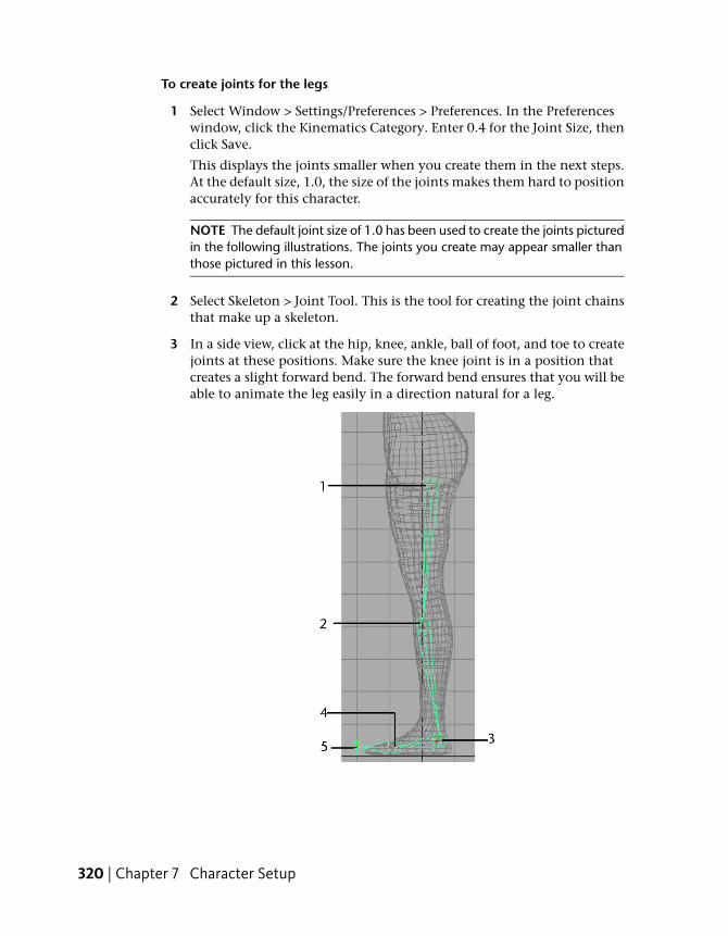
To create joints for the legs
1 Select Window > Settings/Preferences > Preferences. In the Preferenceswindow, click the Kinematics Category. Enter 0.4 for the Joint Size, thenclick Save.
This displays the joints smaller when you create them in the next steps.At the default size, 1.0, the size of the joints makes them hard to positionaccurately for this character.
NOTE The default joint size of 1.0 has been used to create the joints picturedin the following illustrations. The joints you create may appear smaller thanthose pictured in this lesson.
2 Select Skeleton > Joint Tool. This is the tool for creating the joint chainsthat make up a skeleton.
3 In a side view, click at the hip, knee, ankle, ball of foot, and toe to createjoints at these positions. Make sure the knee joint is in a position thatcreates a slight forward bend. The forward bend ensures that you will beable to animate the leg easily in a direction natural for a leg.
320 | Chapter 7 Character Setup
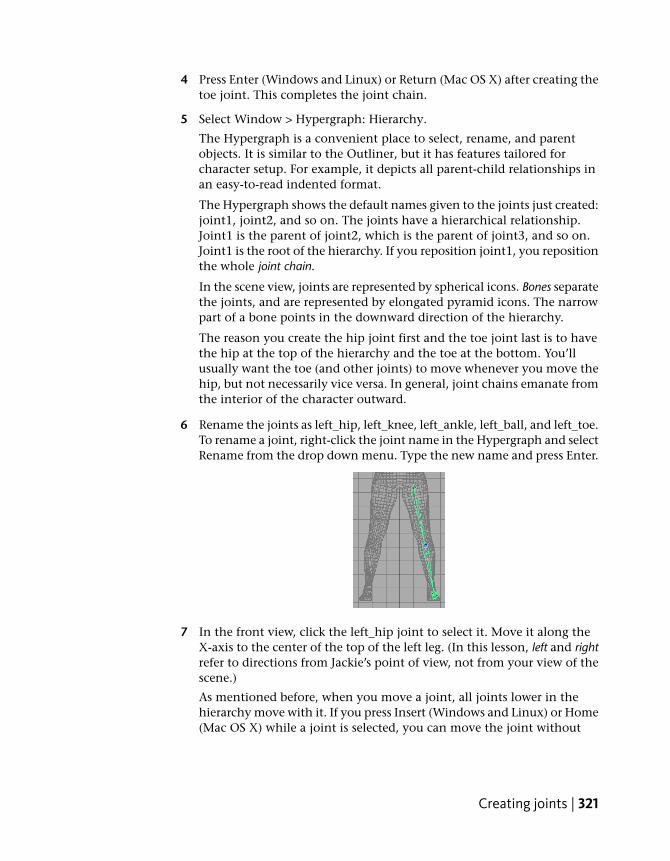
4 Press Enter (Windows and Linux) or Return (Mac OS X) after creating thetoe joint. This completes the joint chain.
5 Select Window > Hypergraph: Hierarchy.
The Hypergraph is a convenient place to select, rename, and parentobjects. It is similar to the Outliner, but it has features tailored forcharacter setup. For example, it depicts all parent-child relationships inan easy-to-read indented format.
The Hypergraph shows the default names given to the joints just created:joint1, joint2, and so on. The joints have a hierarchical relationship.Joint1 is the parent of joint2, which is the parent of joint3, and so on.Joint1 is the root of the hierarchy. If you reposition joint1, you repositionthe whole joint chain.
In the scene view, joints are represented by spherical icons. Bones separatethe joints, and are represented by elongated pyramid icons. The narrowpart of a bone points in the downward direction of the hierarchy.
The reason you create the hip joint first and the toe joint last is to havethe hip at the top of the hierarchy and the toe at the bottom. You’llusually want the toe (and other joints) to move whenever you move thehip, but not necessarily vice versa. In general, joint chains emanate fromthe interior of the character outward.
6 Rename the joints as left_hip, left_knee, left_ankle, left_ball, and left_toe.To rename a joint, right-click the joint name in the Hypergraph and selectRename from the drop down menu. Type the new name and press Enter.
7 In the front view, click the left_hip joint to select it. Move it along theX-axis to the center of the top of the left leg. (In this lesson, left and rightrefer to directions from Jackie’s point of view, not from your view of thescene.)
As mentioned before, when you move a joint, all joints lower in thehierarchy move with it. If you press Insert (Windows and Linux) or Home(Mac OS X) while a joint is selected, you can move the joint without
Creating joints | 321
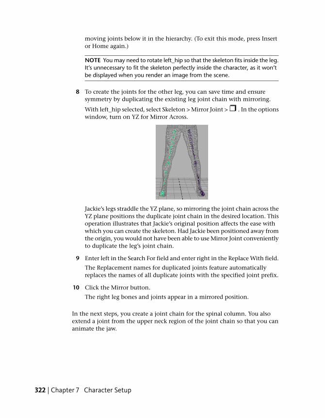
moving joints below it in the hierarchy. (To exit this mode, press Insertor Home again.)
NOTE You may need to rotate left_hip so that the skeleton fits inside the leg.It’s unnecessary to fit the skeleton perfectly inside the character, as it won’tbe displayed when you render an image from the scene.
8 To create the joints for the other leg, you can save time and ensuresymmetry by duplicating the existing leg joint chain with mirroring.
With left_hip selected, select Skeleton > Mirror Joint > . In the optionswindow, turn on YZ for Mirror Across.
Jackie’s legs straddle the YZ plane, so mirroring the joint chain across theYZ plane positions the duplicate joint chain in the desired location. Thisoperation illustrates that Jackie’s original position affects the ease withwhich you can create the skeleton. Had Jackie been positioned away fromthe origin, you would not have been able to use Mirror Joint convenientlyto duplicate the leg’s joint chain.
9 Enter left in the Search For field and enter right in the Replace With field.
The Replacement names for duplicated joints feature automaticallyreplaces the names of all duplicate joints with the specified joint prefix.
10 Click the Mirror button.
The right leg bones and joints appear in a mirrored position.
In the next steps, you create a joint chain for the spinal column. You alsoextend a joint from the upper neck region of the joint chain so that you cananimate the jaw.
322 | Chapter 7 Character Setup
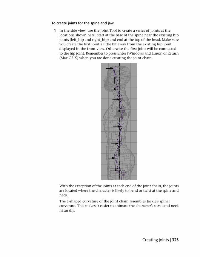
To create joints for the spine and jaw
1 In the side view, use the Joint Tool to create a series of joints at thelocations shown here. Start at the base of the spine near the existing hipjoints (left_hip and right_hip) and end at the top of the head. Make sureyou create the first joint a little bit away from the existing hip jointdisplayed in the front view. Otherwise the first joint will be connectedto the hip joint. Remember to press Enter (Windows and Linux) or Return(Mac OS X) when you are done creating the joint chain.
With the exception of the joints at each end of the joint chain, the jointsare located where the character is likely to bend or twist at the spine andneck.
The S-shaped curvature of the joint chain resembles Jackie’s spinalcurvature. This makes it easier to animate the character’s torso and necknaturally.
Creating joints | 323

2 Starting at the base of the spine, name the joints back_root, pelvis,lower_back, mid_back, upper_back, lower_neck, upper_neck, and crown.
3 To set up the skeleton for jaw movement, extend a joint from theupper_neck joint. With the Joint Tool selected, click the upper_neck jointin the Hypergraph to select it, then click to create a new joint near thelips, and press Enter or Return. Name the new joint as jaw.
Creating joints for the arms is similar to creating joints for the legs.
To create joints for the arms
1 In the front view, create a series of joints at the locations shown in thefigure. Start at the pectoral region (near the upper_back joint) and endat the wrist.
2 Name the joints left_arm_root, left_shoulder, left_elbow, and left_wrist.
3 In the top view, select the left_elbow joint, select the Move tool, pressInsert (Windows and Linux) or Home (Mac OS X), then move the jointto the back of the arm. Press Insert or Home again.
324 | Chapter 7 Character Setup

Moving the joint to the back of the arm creates a bend at the elbow. Thiswill make it easier to animate the character’s arm in the direction an armnaturally bends.
4 In the perspective view, select left_arm_root. Select Skeleton > MirrorJoint. This creates a copy of the left arm’s joint chain for the right armand renames them in the process.
The right arm bones and joints appear in a mirrored position.
Adding joints to a skeletonWhen you bind a character to a skeleton (described in the next lesson), theskeleton provides a structure for the character’s skin and prevents the skinfrom collapsing as you pose the skeleton.
It’s useful to add extra joints in areas of the character where you want thesurface to keep its volume upon deformation. In the next steps, you’ll addribs to Jackie’s skeleton. Although you will not bind the character in thislesson, the technique of adding ribs is important to learn so that when youdo bind a character, the skin in the torso area will not collapse as you pose
Adding joints to a skeleton | 325
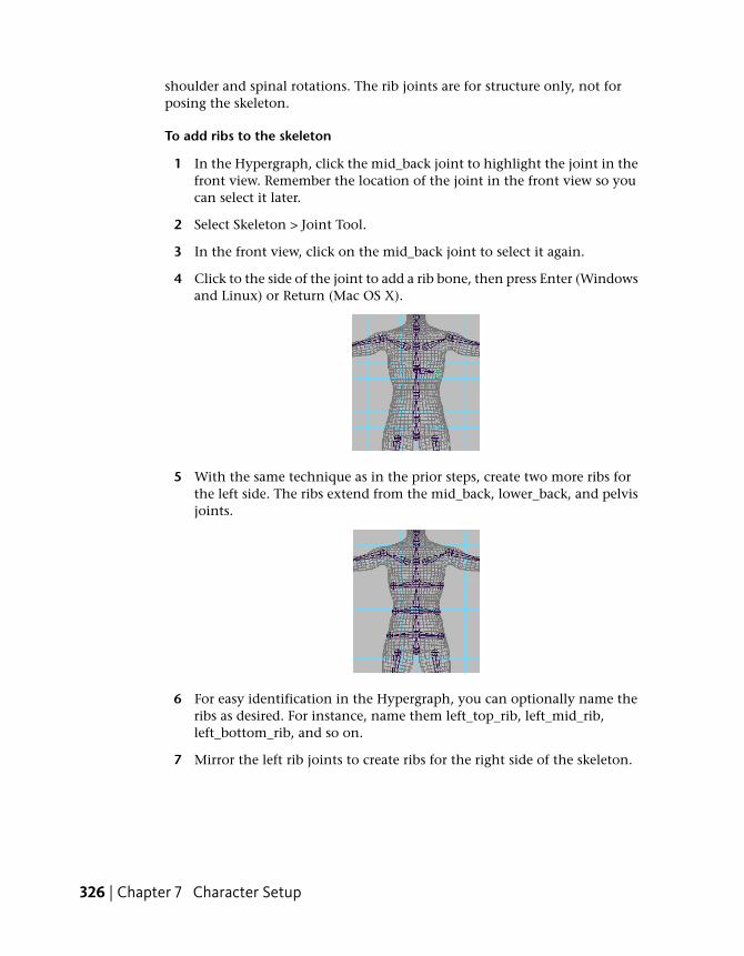
shoulder and spinal rotations. The rib joints are for structure only, not forposing the skeleton.
To add ribs to the skeleton
1 In the Hypergraph, click the mid_back joint to highlight the joint in thefront view. Remember the location of the joint in the front view so youcan select it later.
2 Select Skeleton > Joint Tool.
3 In the front view, click on the mid_back joint to select it again.
4 Click to the side of the joint to add a rib bone, then press Enter (Windowsand Linux) or Return (Mac OS X).
5 With the same technique as in the prior steps, create two more ribs forthe left side. The ribs extend from the mid_back, lower_back, and pelvisjoints.
6 For easy identification in the Hypergraph, you can optionally name theribs as desired. For instance, name them left_top_rib, left_mid_rib,left_bottom_rib, and so on.
7 Mirror the left rib joints to create ribs for the right side of the skeleton.
326 | Chapter 7 Character Setup

Creating a skeleton hierarchySo far you have created five separate joint chains: one for the spine, and onefor each arm and each leg. You need to create a single hierarchy from the fivejoint chains so you can move all of them as a single unit. To create the singlehierarchy, you parent the arms and legs to the nearest joint in the spine.
To parent the arm and leg joint chains to the spine
1 In the Hypergraph, use the middle mouse button to drag left_arm_rootto upper_back.
When you parent one joint to another, Maya creates a bone that connectsthe parent to the child. In this case, the bone connects upper_back toleft_arm_root.
2 Use the middle mouse button to drag right_arm_root to upper_back.
3 Use the middle mouse button to drag left_hip to back_root.
4 Use the middle mouse button to drag right_hip to back_root.
Now if you need to move the entire skeleton, you can moveback_root—the root of the hierarchy. The completed skeleton is shownin the following figure (with Jackie hidden):
Forward and inverse kinematicsThere are two techniques for posing a skeleton: forward kinematics and inversekinematics.
Creating a skeleton hierarchy | 327

Forward kinematics (FK)
To pose a character with forward kinematics, you rotate each joint individuallyuntil you get the desired positioning. For example, to move a hand to somelocation, you must rotate several arm joints to reach the location.
When you animate a skeleton posed with forward kinematics, Mayainterpolates the joint rotations starting with the root joint, then the root’schild joints, and so on down through the skeleton’s action hierarchy. Mayaproceeds forward through the action hierarchy, starting at the root joint.
Forward kinematics is intuitive for creating simple arc motions, but it’s tediousif you are animating a complex skeleton. It’s also not intuitive for specifyinggoal-directed motion. For example, to move a hand to some location, it’s notobvious how to rotate the joints in an arm.
Inverse kinematics (IK)
With IK, you create an extra control structure, an IK handle, for certain jointchains such as arms and legs. An IK handle lets you pose and animate an entirejoint chain by moving a single manipulator.
As you pose the IK handle, it automatically rotates all the joints in the jointchain. For example, if you move a hand to a doorknob, the other joints in thearm rotate to accommodate the hand’s new positioning.
IK is more intuitive than forward kinematics for goal-directed motion becauseyou can focus on the goal rather than on how you need to rotate each jointto achieve that goal.
Posing and animating using inverse kinematicsNext, you create IK handles that you’ll later use to pose the arms and legs.The next steps describe some initial setup you should perform before creatingthe IK handles.
To set up the character prior to creating IK handles
1 Select the root of the hierarchy, back_root, and then select Skeleton > SetPreferred Angle.
This sets the current joint angles throughout the skeleton as the preferredangles. This is a useful step after you complete a skeleton. Maya thereafteruses the current bend in the knees and elbows as the preferred initialrotation direction of these joints during inverse kinematics (IK) posing.
328 | Chapter 7 Character Setup
This makes it easier to pose the character with motion that is natural fora human character.
2 Select Jackie in the Outliner and, from the main menu, select Display >Hide > Hide Selection. (You must select Jackie from the Outliner becauseJackie is a template object.) By hiding Jackie, you’ll lessen scene clutteras you pose the skeleton in the following steps.
To create, pose, and animate IK handles for the legs
1 Select Skeleton > IK Handle Tool > .
2 In the Tool Settings window, make sure Current Solver is set to ikRPsolver.
This type of IK solver has characteristics that work well for thisapplication.
3 In the perspective view, click left_hip and left_ankle.
This creates an IK handle that lets you control all joints from left_hipthrough left_ankle. The handle’s main manipulator is at the left_ankle.
The IK handle is the selected object after you create it. If youunintentionally cancel the selection of the handle, you can select it againby clicking the left_ankle—the last joint you clicked after using the IKHandle Tool. Whenever you select a handle, make sure you do not selectjoints or other objects along with the handle. You can check the Outlinerto confirm your selection.
4 Go to the start of the playback range.
5 With the IK handle selected, select Animate > Set Key to key the leg’scurrent position at the first frame.
6 Go to frame 12.
7 In the side view, use the Move tool to drag the IK handle up and to theleft, as if Jackie were stepping up a staircase. The foot and knee movewhile the hip stays in place.
Posing and animating using inverse kinematics | 329
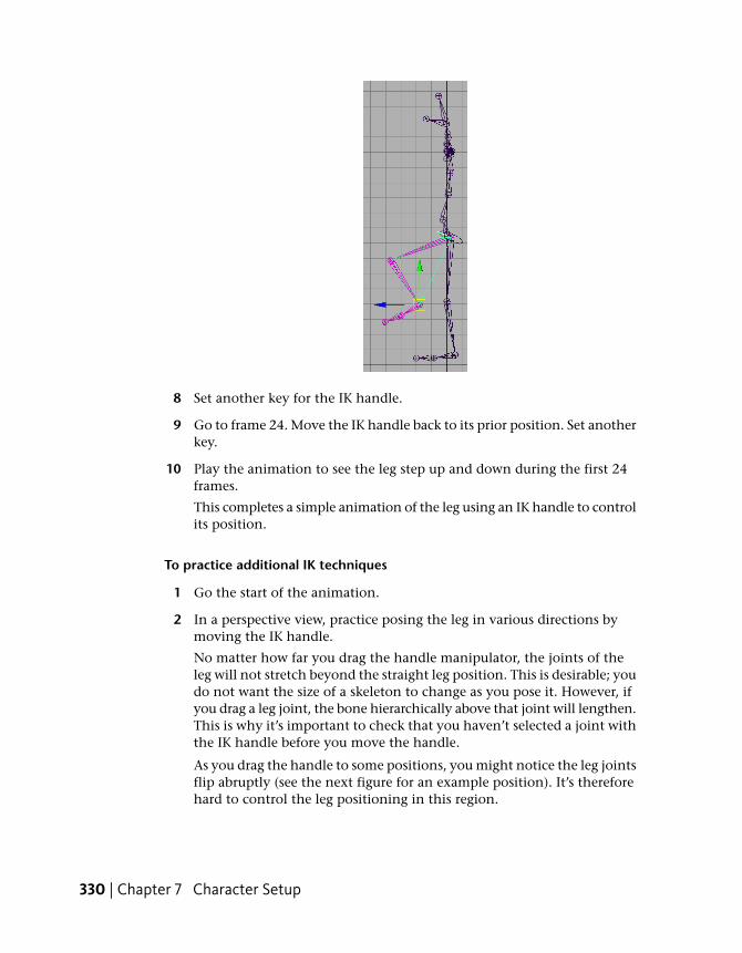
8 Set another key for the IK handle.
9 Go to frame 24. Move the IK handle back to its prior position. Set anotherkey.
10 Play the animation to see the leg step up and down during the first 24frames.
This completes a simple animation of the leg using an IK handle to controlits position.
To practice additional IK techniques
1 Go the start of the animation.
2 In a perspective view, practice posing the leg in various directions bymoving the IK handle.
No matter how far you drag the handle manipulator, the joints of theleg will not stretch beyond the straight leg position. This is desirable; youdo not want the size of a skeleton to change as you pose it. However, ifyou drag a leg joint, the bone hierarchically above that joint will lengthen.This is why it’s important to check that you haven’t selected a joint withthe IK handle before you move the handle.
As you drag the handle to some positions, you might notice the leg jointsflip abruptly (see the next figure for an example position). It’s thereforehard to control the leg positioning in this region.
330 | Chapter 7 Character Setup
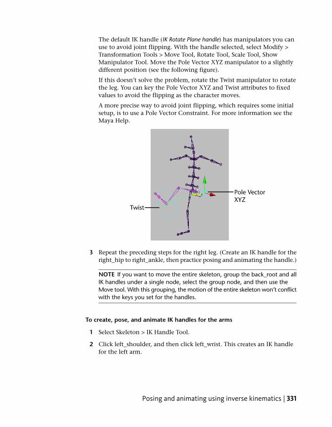
The default IK handle (IK Rotate Plane handle) has manipulators you canuse to avoid joint flipping. With the handle selected, select Modify >Transformation Tools > Move Tool, Rotate Tool, Scale Tool, ShowManipulator Tool. Move the Pole Vector XYZ manipulator to a slightlydifferent position (see the following figure).
If this doesn’t solve the problem, rotate the Twist manipulator to rotatethe leg. You can key the Pole Vector XYZ and Twist attributes to fixedvalues to avoid the flipping as the character moves.
A more precise way to avoid joint flipping, which requires some initialsetup, is to use a Pole Vector Constraint. For more information see theMaya Help.
3 Repeat the preceding steps for the right leg. (Create an IK handle for theright_hip to right_ankle, then practice posing and animating the handle.)
NOTE If you want to move the entire skeleton, group the back_root and allIK handles under a single node, select the group node, and then use theMove tool. With this grouping, the motion of the entire skeleton won’t conflictwith the keys you set for the handles.
To create, pose, and animate IK handles for the arms
1 Select Skeleton > IK Handle Tool.
2 Click left_shoulder, and then click left_wrist. This creates an IK handlefor the left arm.
Posing and animating using inverse kinematics | 331

3 Select Skeleton > IK Handle Tool.
4 Click right_shoulder, then click right_wrist. This creates an IK handle forthe right arm.
5 Practice posing and animating the handles.
Posing and animating using forward kinematicsAs the last part of the lesson, you can optionally practice posing and animatingthe character by rotating joints that are not controlled by IK handles—theball joints of the feet, and joints from the back_root through the upper_neck.Rotating such joints is forward kinematics.
With the exception of the back_root, you’ll invariably rotate rather than movethe joints that aren’t part of an IK handle. If you move the joints, the boneslengthen. This deforms bound skin undesirably unless you are creatingcartoon-like distortions.
Because you’ve already set keys for IK handles, some joint rotations on non-IKhandle joints will be restrained by the IK handle positioning. If this interfereswith the intended poses, you can remove all prior animation from an IK handleby selecting Edit > Keys > Delete Keys. You can also use Delete Keys to removeall animation from keys you’ve set with forward kinematics.
Beyond the lessonIn this lesson you learned how to:
■ Create a skeleton with bones and joints.
■ Pose the skeleton using Inverse Kinematics.
Additional things to consider when working with skeletons:
■ The appropriate number of joints in a skeleton depends on the anatomicalparts of the character you want to manipulate. More joints means finercontrol at the expense of greater complexity.
■ As you created the skeleton in this lesson, you ended the arm’s joint chainat the wrist. This prevents you from animating hand motion. If you needto animate hand motion or even finger motion, you would need to makeadditional joints and IK handles. The same applies to foot and toe motion.
332 | Chapter 7 Character Setup
■ When you create a skeleton, you can animate a character bound to it toproduce natural skin deformations. Although you animated an unskinnedskeleton in this lesson, it’s more common to animate a skinned skeleton.Binding a character is the topic of the next lesson.
■ It’s typically best to animate the entire skeleton from pose to pose at desiredframes. It’s hard to get desired results by animating one limb for a framerange, another limb for a frame range, and so on.
There are many other ways to work with skeletons not described in this lesson:
■ You can blend or switch between IK and forward kinematics on jointscontrolled by an IK handle.
■ There are other types of IK handles that provide different controls formanipulating parts of a skeleton. Especially noteworthy is the IK splinehandle, which makes it easy to animate the twisting, wavy motion in tails,necks, spines, snakes, and so on.
For more details on these and other features, please refer to the Maya Help.
Lesson 2: Smooth skinning
IntroductionAfter you create a skeleton, you bind it with the character’s surface so that thesurfaces move with the skeleton during animation. Binding is also calledskinning, and a character’s surface after binding is called a skin.
It is important that the character’s skin deforms naturally as the skeletonmoves. Near joints, the skin bulges or indents when you rotate the joints.
In Maya, the skin deforms because the surface’s vertices (or CVs) move inresponse to the rotation of adjacent joints. The vertices are known as skinpoints. This is useful for animating elbows, shoulders, necks, and so on.
By default, the influence a joint has on a skin point’s movement depends onhow close it is to that joint. You can edit skin point weighting to change thedefault movement.
In this lesson you learn how to:
■ Bind a skeleton using a smooth bind technique.
Lesson 2: Smooth skinning | 333

■ View and modify skin weights using the Skin Weights Tool.
■ Use influence objects to enhance the skin deformation of a character.
Open the scene for the lesson
In this lesson, you work with a scene we created for your use. The scenecontains a human character and skeleton. Each leg and arm of the skeletonhas an IK handle that lets you pose the limbs conveniently. If you completedthe prior lesson, the character, skeleton, and IK handles will be familiar.
1 Make sure you’ve done the steps in Preparing for the lessons on page 318.
2 Open the scene file named SmoothSkin.mb.
This file can be found in the GettingStarted directory that you set asyour Maya project: GettingStarted/CharSetup.mb.
The character in the scene, Jackie, is displayed in a transparent fashionso you can see the skeleton beneath the surface.
Smooth binding a skeletonYou use Jackie as the surface to be bound to the skeleton.
To bind the skeleton using smooth skinning
1 Select Jackie.
2 Shift-select the back_root joint.
334 | Chapter 7 Character Setup
The back_root joint is at the base of Jackie’s spine. If you are not surewhich joint it is, select it in the Hypergraph (Window > Hypergraph:Hierarchy).
3 Select Skin > Bind Skin > Smooth Bind > .
The Smooth Bind Options window appears.
4 In the Smooth Bind Options window, set Max Influences to 3, then clickBind Skin.
A Max Influences value of 3 specifies that three joints influence each skinpoint. By default, the joint closest to the point has the most influence.The second most influential joint is that joint’s parent or child joint,whichever is closest to the point. The third most influential joint is thenearest parent or child of the second joint. The influence drops with thedistance from the joints. The amount of influence each joint has on anyskin point is the skin weight.
The default skin weights create smooth deformations of the skin at elbows,knees, and elsewhere as the nearby joints rotate.
5 Select and move any or all of the four IK handles to pose the arms andlegs in various positions in order to get used to posing with the IK handles.
To select an IK handle, drag a selection box around a wrist or ankle joint.To move a handle, use the Move tool to drag the handle in the desireddirection.
Note that you can also select the IK handles in the Hypergraph. Thehandles are indented under jackieSkeleton. Each is named for a leg orarm, for example, ikHandleLeftLeg. For more details on IK handles, seeLesson 1: Skeletons and kinematics on page 318.
6 If you prefer to turn off the skin’s transparency so you can see the skinmore clearly, turn off Shading > X-Ray. Do not be concerned that theskeleton pokes through the skin, as the skeleton is not displayed in arendered image.
As you pose the arms and legs, examine the skin in the regions wherejoints bend. For many poses, the skin looks natural. For others, the skinfolds, compresses, or bulges unnaturally. The pelvis, shoulders, and torsoare common problem areas for various poses. For example, if you movean arm straight up, the shoulder compresses as in the following figure.
Smooth binding a skeleton | 335

There are two ways to improve the smooth skin deformations:
■ Add an influence object to eliminate collapsing regions or to create musclebulge. For example, you can use an influence object to make the shoulderregion look more natural in the prior pose.
■ Edit skin weights—to remove minor lumps or indented regions. Forexample, you can fill out an undesirable concave region at the chest thatappears when you move the arm to certain poses.The following procedures explain the techniques.
Skin weighting and deformationsIn the next steps, you’ll learn how joints and skin weights influencedeformations at Jackie’s chest. In a subsequent section, you’ll improve unevendeformations.
To see how skin weights affect a skin’s deformation
1 Pose the left arm similar to the following figure. The left breast becomesirregularly shaped.
336 | Chapter 7 Character Setup

2 Select Jackie.
3 Select Skin > Edit Smooth Skin > Paint Skin Weights Tool > .
4 In the Influence list of the Tool Settings window, select any joint, forinstance, pelvis. The grayscale color of Jackie’s skin indicates how muchinfluence that joint has on the skin’s deformation.
White means the skin is maximally influenced by the joint. Black meansthe skin is not influenced by the joint. Gray means the influence is partial.The lighter the gray, the more the influence.
Each point on the surface is influenced by three joints, as specified bythe Max Influence setting in a prior step. However, one or two of thethree joints might have so little influence as to be insignificant.
In general, a white region of skin is influenced nearly entirely by the jointselected in the Influence section of the Tool Settings window. A grayregion is influenced significantly by one or two additional joints.
The reason the left breast becomes irregularly shaped as you pose the armis that some joint is exerting too much or too little influence on thebreast.
5 Select each entry in the Influence list to determine which joints areinfluencing the irregular region of the breast. The region will be a shadeof gray (or white) when you select the appropriate joints. Theleft_arm_root is the main influence. The upper_back, mid_back, andleft_top_rib also have influence, though not exactly in the same region.
Skin weighting and deformations | 337

Modifying skin weightsYou can modify the skin weights for any of the influencing joints to alter theirregular region. If you don’t get the desired results when you change the skinweights of one of the influencing joints, you can undo your changes and tryanother influencing joint.
In general, it’s best to modify the skin weights of the most influential jointfirst, then work with less influential joints if you don’t get the desired results.Modifying skin weights requires experimentation.
In the next steps, you’ll modify the skin weights for the left_arm_root joint.
To modify skin weights using the Paint Skin Weights Tool
1 Select left_arm_root in the Influence list.
2 In the Paint Weights Menu section of the window, set Value to 0.1 andturn on Add.
3 Drag the mouse pointer to paint the irregular region of the breast. Eachstroke adds 0.1 (10%) to the skin weight. The weight for a skin point hasa maximum value of 1 (fully white).
TIP Painting skin weights using a tablet with stylus allows you to takeadvantage of pressure sensitivity.
Repeat the strokes several times until the irregular region becomessmoother. The jagged, asymmetrical wireframe at the breast becomesmore symmetrical as the skin becomes smoother. The region whitens,which indicates increased influence from the left_arm_root joint. Notethat increasing the influence of one joint lessens the influence of theother influencing joints.
4 To check the shape with full-color shading, click the Select Tool. (Youmight also prefer to cancel the selection of Jackie to eliminate the displayof the highlighted wireframe.)
338 | Chapter 7 Character Setup
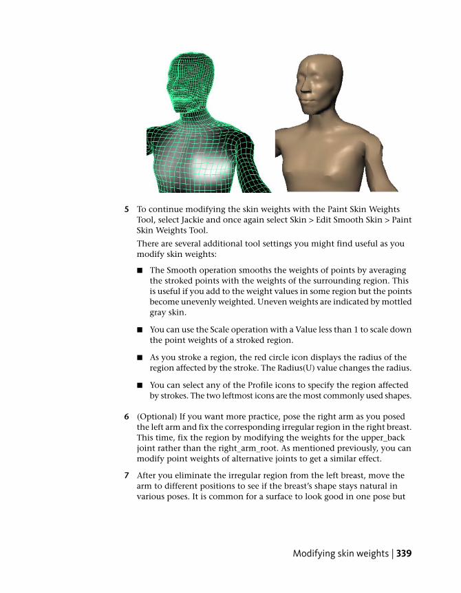
5 To continue modifying the skin weights with the Paint Skin WeightsTool, select Jackie and once again select Skin > Edit Smooth Skin > PaintSkin Weights Tool.
There are several additional tool settings you might find useful as youmodify skin weights:
■ The Smooth operation smooths the weights of points by averagingthe stroked points with the weights of the surrounding region. Thisis useful if you add to the weight values in some region but the pointsbecome unevenly weighted. Uneven weights are indicated by mottledgray skin.
■ You can use the Scale operation with a Value less than 1 to scale downthe point weights of a stroked region.
■ As you stroke a region, the red circle icon displays the radius of theregion affected by the stroke. The Radius(U) value changes the radius.
■ You can select any of the Profile icons to specify the region affectedby strokes. The two leftmost icons are the most commonly used shapes.
6 (Optional) If you want more practice, pose the right arm as you posedthe left arm and fix the corresponding irregular region in the right breast.This time, fix the region by modifying the weights for the upper_backjoint rather than the right_arm_root. As mentioned previously, you canmodify point weights of alternative joints to get a similar effect.
7 After you eliminate the irregular region from the left breast, move thearm to different positions to see if the breast’s shape stays natural invarious poses. It is common for a surface to look good in one pose but
Modifying skin weights | 339

not in another. Strive to make the surface look good in the poses thatyou are likely to use during animation.
Influence objectsYou can create an object and use it to influence the shape of smooth skin.The object, called an influence object, acts like a surgical implant againstwhich the skin deforms. For example, you can create a sphere and use it tosimulate a muscle or bone that bulges as you pose the character in certainpositions. You can also use an influence object to smooth deformation andmaintain volume in regions that collapse while bending.
In the next steps, you’ll use a sphere as an influence object to simulate anelbow jutting out as Jackie’s arm bends. To use an influence object, the skeletonmust be in the bind pose—the original pose at which the skin was bound toJackie.
To return the skeleton to the bind pose
1 Click the Select Tool and cancel the selection of Jackie.
2 Turn off Modify > Evaluate Nodes > IK Solvers.
After you use an IK handle to pose a character, you must do this stepbefore you can return the skeleton to the bind pose.
3 Select back_root, the root of the skeleton.
4 Select Skin > Go To Bind Pose.
5 Select the ikHandleLeftArm in the Hypergraph. Use the Move Tool tomove the handle manipulator slightly in any direction. When you releasethe mouse, note that the arm does not move and that the IK handlemanipulator snaps back to the desired position at the end of the jointchain. Repeat this step for any other IK handles you posed previously.
340 | Chapter 7 Character Setup

6 Turn on Modify > Evaluate Nodes.
You must do this step to enable the IK solvers so you can manipulate IKhandles in the scene again.
To position a sphere to be used as an influence object
1 Right-click Jackie’s surface (anywhere but on the skeleton) and selectActions > Template from the marking menu.
By making Jackie a template, you won’t accidentally select Jackie insubsequent steps.
2 Create a sphere (select Create > Polygon Primitives > Sphere >) and nameit elbow_influence.
3 Scale the sphere to be slightly smaller than any of Jackie’s joints (seeillustration below).
4 Move the sphere so that its surface is positioned where the elbow wouldjut out, but still within the skin. You can optionally reshape the sphere’scurvature to resemble the tip of an elbow jutting out from a bent arm.For example, you can scale the sphere in one dimension to squash itsshape or you can move individual vertices. A top view of the sphere’sshape and position follows:
The exact position and scale of the sphere is unimportant. You can makeslight position and scale adjustments later to enhance the deformationsthat result from its use.
To make the sphere an influence object
1 In the Hypergraph, select Jackie and Shift-select elbow_influence.
2 Select Skin > Edit Smooth Skin > Add Influence > . In the Add InfluenceOptions, select Edit > Reset Settings, and then click the Add button.
Maya completes the operation within a few moments. To ensure theinfluence object stays in the correct position at the elbow, you will parentit to the left_shoulder joint.
Influence objects | 341

3 In the Hypergraph, Shift-select elbow_influence, elbow_influenceBase,and left_shoulder joint, in that order.
The order of selection is important. The parent object should be selectedlast.
4 Press p to parent the elbow nodes under the left_shoulder joint.
The elbow_influence nodes appear in the skeleton hierarchy below theleft_shoulder joint.
The elbow_influenceBase is known as a base object. It stores vertexposition information for the influence object. The reason for parentingthe base object to the left_shoulder joint is so that the influence object’svertices stay in the correct position at the elbow whenever the elbowmoves to a new position. Other than this step, you do not work with thebase object.
5 Right-click Jackie and select Actions > Untemplate. It is easier to seesubsequent skin deformations when Jackie is displayed with smoothshading rather than as a template.
6 From the menus at the top of the top view, turn off Show > Joints toavoid having the joints obstruct your view of the skin.
7 Use each arm’s IK handle (ikHandle1 and ikHandle2) to pose the armsin the following position.
The left elbow looks more natural than the right elbow. To tune theelbow’s deformation during bending, change the position, scale, androtation of elbow_influence.
Do not be concerned if the influence object pokes through the skin. Itwon’t be displayed when you render the animation.
342 | Chapter 7 Character Setup

Beyond the lessonIn this lesson you learned how to:
■ Bind a skeleton to a single surface.You can bind a skeleton to multiple surfaces or even to a selection ofpolygonal vertices or NURBS CVs or subdivision surfaces.
■ Use the Paint Skin Weights Tool to prevent a region from collapsing upondeformation.To control skin weights with more precision than shown in the lesson,you can modify skin weights numerically with the Window > GeneralEditors > Component Editor. If you smooth skin multiple surfaces whichhave been seamed together, there are many tool settings for the Paint SkinWeights Tool that make the task easier.
■ Use an influence object to make an elbow stick out upon bending.Another common use of an influence object is to simulate a muscle bulgingduring joint rotation. The technique requires use of Set Driven Key to linkthe bulging influence object’s scale values to the rotation of the appropriatejoint. A brief example of this technique is in the Maya Help for SmoothSkin.
Skin weights and influence objects cannot overcome all modeling problems.For instance, if you further separate Jackie’s legs sideways, you will see anundesirable fold at the hips. This occurs because of the asymmetricalarrangement of polygonal edges in the hip region of the original model. Tofix the problem, you would need to detach the skin, alter the original model,then smooth bind the model again.
Maya has an alternative skinning method, rigid skinning, which gives resultssimilar to smooth skinning but requires use of different enhancement tools:flexor and lattice deformers. In general, smooth skinning gives more naturaldeformations with less effort than rigid skinning. If you skin multiple seamedsurfaces, however, processing is faster with rigid skinning than with smoothskinning.
Smooth skinning is just one of the techniques for perfecting a character’sdeformations during animation. You can use Maya’s other deformers aloneor in addition to smooth skinning to achieve the results you want.
For more information, please refer to Smooth skinning in the Maya Help.
Beyond the lesson | 343

Lesson 3: Cluster and blend shape deformers
IntroductionFacial animation is an integral component of character animation. The faceof a character can be animated to impart a range of emotions and expressions.Maya has two deformation tools that ease character setup for facial animation:cluster deformers and blend shape.
Cluster deformers enable you to control a set of an object's points (CVs,vertices, or lattice points) with varying amounts of influence to create a targetshape for an animation.
A Blend Shape deformer provides an interface for blending between varioustarget shapes, to control the range of movement for the cluster on an objector face.
In this lesson, you will be introduced to cluster deformers in order to shapea characters mouth into a smile pose. You will learn to use the Blend Shapefeature so you can animate the face from a neutral pose to a smile. In thislesson, you learn how to:
■ Select CVs in a region and create a cluster deformer.
■ Use the cluster deformer handle to adjust the position of a cluster deformer.
■ Use the Paint Cluster Weights Tool to refine the cluster weight values.
■ Create a Blend Shape deformer to control the blending between targetshapes.
Open the scene for the lessonIn this lesson, you’ll work with a scene we created for your use.
1 Make sure you’ve done the steps in Preparing for the lessons on page 318.
2 Open the scene file named ClusterBS.mb.
This file can be found in the GettingStarted directory that you set asyour Maya project: GettingStarted/CharSetup.
344 | Chapter 7 Character Setup
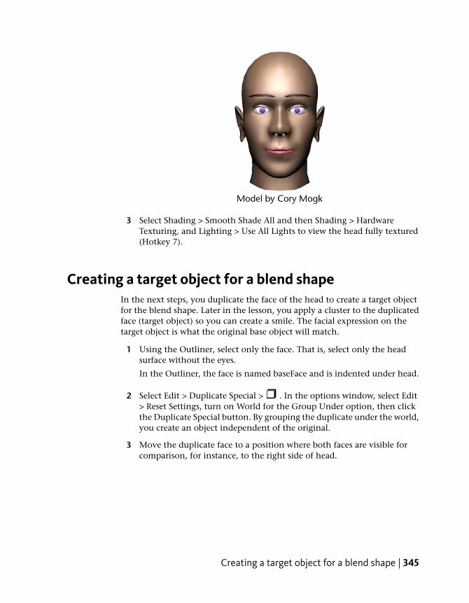
3 Select Shading > Smooth Shade All and then Shading > HardwareTexturing, and Lighting > Use All Lights to view the head fully textured(Hotkey 7).
Creating a target object for a blend shapeIn the next steps, you duplicate the face of the head to create a target objectfor the blend shape. Later in the lesson, you apply a cluster to the duplicatedface (target object) so you can create a smile. The facial expression on thetarget object is what the original base object will match.
1 Using the Outliner, select only the face. That is, select only the headsurface without the eyes.
In the Outliner, the face is named baseFace and is indented under head.
2 Select Edit > Duplicate Special > . In the options window, select Edit> Reset Settings, turn on World for the Group Under option, then clickthe Duplicate Special button. By grouping the duplicate under the world,you create an object independent of the original.
3 Move the duplicate face to a position where both faces are visible forcomparison, for instance, to the right side of head.
Creating a target object for a blend shape | 345
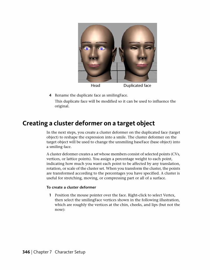
4 Rename the duplicate face as smilingFace.
This duplicate face will be modified so it can be used to influence theoriginal.
Creating a cluster deformer on a target objectIn the next steps, you create a cluster deformer on the duplicated face (targetobject) to reshape the expression into a smile. The cluster deformer on thetarget object will be used to change the unsmiling baseFace (base object) intoa smiling face.
A cluster deformer creates a set whose members consist of selected points (CVs,vertices, or lattice points). You assign a percentage weight to each point,indicating how much you want each point to be affected by any translation,rotation, or scale of the cluster set. When you transform the cluster, the pointsare transformed according to the percentages you have specified. A cluster isuseful for stretching, moving, or compressing part or all of a surface.
To create a cluster deformer
1 Position the mouse pointer over the face. Right-click to select Vertex,then select the smilingFace vertices shown in the following illustration,which are roughly the vertices at the chin, cheeks, and lips (but not thenose):
346 | Chapter 7 Character Setup
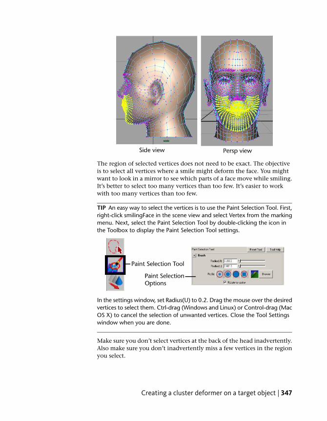
The region of selected vertices does not need to be exact. The objectiveis to select all vertices where a smile might deform the face. You mightwant to look in a mirror to see which parts of a face move while smiling.It’s better to select too many vertices than too few. It’s easier to workwith too many vertices than too few.
TIP An easy way to select the vertices is to use the Paint Selection Tool. First,right-click smilingFace in the scene view and select Vertex from the markingmenu. Next, select the Paint Selection Tool by double-clicking the icon inthe Toolbox to display the Paint Selection Tool settings.
In the settings window, set Radius(U) to 0.2. Drag the mouse over the desiredvertices to select them. Ctrl-drag (Windows and Linux) or Control-drag (MacOS X) to cancel the selection of unwanted vertices. Close the Tool Settingswindow when you are done.
Make sure you don’t select vertices at the back of the head inadvertently.Also make sure you don’t inadvertently miss a few vertices in the regionyou select.
Creating a cluster deformer on a target object | 347

2 Select Create Deformers > Cluster.
This puts the vertices into a cluster—a set of points you can move assingle entity. The cluster’s handle appears in the view as a C icon.
3 In the Outliner, make sure the cluster2Handle is selected.
4 Use the Move tool to drag the cluster handle up along its Y-axis a smallamount until smilingFace is deformed as follows:
The cluster set on smilingFace should be slightly higher than the clusteron the original face. This will become the basis for the blend shapedeformer.
Editing cluster weightsIn this section you will use the Paint Cluster Weights Tool to further refinethe smilingFace. As you saw in previous steps, the points in a cluster movewhen you move the cluster handle. The distance a particular point movesdepends on its weight. Lower weights cause less movement, while higherweights cause exaggerated movement. In the next steps, you create a smileby editing the weights.
To edit cluster weights using the Paint Cluster Weights Tool
1 Select smilingFace.
348 | Chapter 7 Character Setup
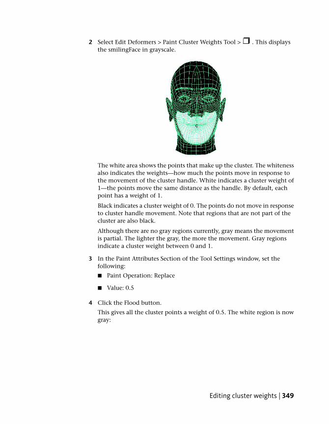
2 Select Edit Deformers > Paint Cluster Weights Tool > . This displaysthe smilingFace in grayscale.
The white area shows the points that make up the cluster. The whitenessalso indicates the weights—how much the points move in response tothe movement of the cluster handle. White indicates a cluster weight of1—the points move the same distance as the handle. By default, eachpoint has a weight of 1.
Black indicates a cluster weight of 0. The points do not move in responseto cluster handle movement. Note that regions that are not part of thecluster are also black.
Although there are no gray regions currently, gray means the movementis partial. The lighter the gray, the more the movement. Gray regionsindicate a cluster weight between 0 and 1.
3 In the Paint Attributes Section of the Tool Settings window, set thefollowing:
■ Paint Operation: Replace
■ Value: 0.5
4 Click the Flood button.
This gives all the cluster points a weight of 0.5. The white region is nowgray:
Editing cluster weights | 349

The selected vertices move down a bit, as the weight of 0.5 lessens theeffect of the prior movement of the cluster by 50%.
5 To check the shape with full-color shading, click the Select Tool. (Youmight also prefer to cancel the selection of smilingFace to eliminate thedisplay of the highlighted wireframe.)
6 To return to the Paint Cluster Weights Tool, select smilingFace and Edit
Deformers > Paint Cluster Weights Tool > again.
7 In the Tool Settings window, set the following
■ Radius(U): 0.1A Radius(U) of 0.1 sets the radius of the region affected by the stroke.The red circle icon on the face displays the radius.
■ Opacity: 0.3An Opacity of 0.3 scales down the effect of painting weight values soyou can build up values gradually with repeated strokes.
■ Paint Operation: ReplaceA Replace operation paints the Value specified on the points stroked.
■ Value: 1A Value of 1 sets the weight value you paint on the points.
8 Paint the region at the corners of the mouth with repeated strokes untilthe face looks roughly like the following figure. If your results differ fromthe figure significantly, undo the strokes and try again.
350 | Chapter 7 Character Setup

While painting weights, it’s useful to intermittently check the shape withwith full-color shading rather than with the grayscale shading. To dothis, click the Select Tool to turn off the Paint Cluster Weights Tool. (Youmight also prefer to cancel the selection of smilingFace to eliminate thedisplay of the highlighted wireframe.)
9 Enter a Value of 0.25 and paint the central region above and below thelips as follows:
Because the corners of the mouth have a high weight and the centralregion around the lips have a low weight, the corners move up more inresponse to the prior positioning of the cluster handle. This creates asmiling mouth. The cheeks and chin have a medium weight, so they also
Editing cluster weights | 351
move up slightly also. (For many people, skin at the chin and neck movesduring smiling.)
10 In the tool settings editor for the Paint Cluster Weights Tool, set the PaintOperation to Smooth. Paint any region where the surface has becomeirregular. Irregular regions are typically indicated by jagged wireframecurves (isoparms) or where a grayscale color makes an abrupt change toa lighter or darker color. Smoothing averages the weights of the strokedpoints with the weights of the surrounding region. The Value setting hasno effect on smoothing.
11 Replace and smooth weights in other regions of the face until you aresatisfied with the smile. For example, you might want to reduce the weightvalues at the side of the nose and immediately below the nose.
Your smilingFace should now have a slight smile as a result of your clusterweight edits.
12 Hide the Paint Attributes Tool settings window.
Creating a blend shapeIn this section, you create a blend shape deformer to control the smile onbaseFace (base object) using the smilingFace (target object). A blend shapedeformer is ideal for facial animation, where you need a number of facialpositions to be readily available for use in an animation sequence. With ablend shape deformer, you can set up a character’s face to blend between asmile, frown, smirk, and so on.
In the next steps, you create a blend shape deformer to change the baseFaceinto the smile of smilingFace.
To create a blend shape deformer
1 In the Outliner, select smilingFace and shift-select baseFace, specificallyin this order.
The smilingFace (the first selection) is called the target object, whilebaseFace (the second selection) is called the base object. The objective ofa blend shape operation is to morph the base shape into the target shape.
2 Select Create Deformers > Blend Shape > .
3 In the Blend Shape node text box, type blendShape, then click Create.
352 | Chapter 7 Character Setup

4 Select Window > Animation Editors > Blend Shape. This displays theBlend Shape editor, which has a slider for changing the base into thetarget shape, and buttons for setting keys.
5 Cancel the selection of the faces so you can see the surfaces without theobscuring highlighted wireframe.
6 Drag the slider from 0 to 1 to morph the baseFace into the target,smilingFace.
Note that you can click the Key button below the slider to set ananimation key for the shape of the face at the current frame. By settinga few keys with different slider values at different points in the timeline,you can animate from the neutral expression to a full or partial smile orvice versa.
When you key the shape, Maya applies the key to the blendShape nodethat was created when you selected Create Deformers > Blend Shape >
. If you need to select the blendShape node, for instance, so you cansee or delete the keys in the Time Slider, click the Select button in theBlend Shape editor.
Creating a blend shape | 353
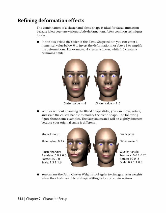
Refining deformation effectsThe combination of a cluster and blend shape is ideal for facial animationbecause it lets you tune various subtle deformations. A few common techniquesfollow.
■ In the box below the slider of the Blend Shape editor, you can enter anumerical value below 0 to invert the deformations, or above 1 to amplifythe deformations. For example, -1 creates a frown, while 1.6 creates abrimming smile:
■ With or without changing the Blend Shape slider, you can move, rotate,and scale the cluster handle to modify the blend shape. The followingfigure shows some examples. The face you created will be slightly differentbecause your original smile is different.
■ You can use the Paint Cluster Weights tool again to change cluster weightswhen the cluster and blend shape editing deforms certain regions
354 | Chapter 7 Character Setup
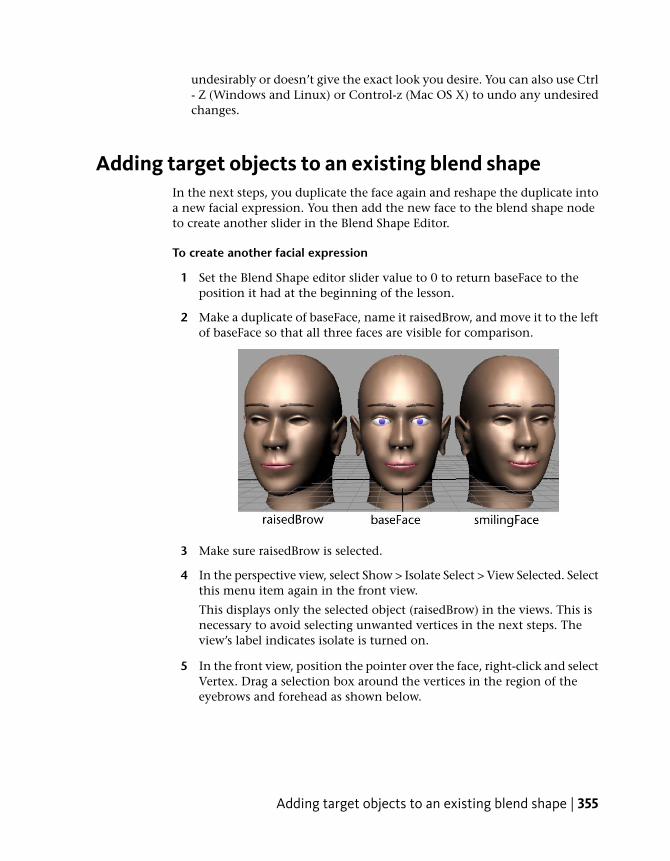
undesirably or doesn’t give the exact look you desire. You can also use Ctrl- Z (Windows and Linux) or Control-z (Mac OS X) to undo any undesiredchanges.
Adding target objects to an existing blend shapeIn the next steps, you duplicate the face again and reshape the duplicate intoa new facial expression. You then add the new face to the blend shape nodeto create another slider in the Blend Shape Editor.
To create another facial expression
1 Set the Blend Shape editor slider value to 0 to return baseFace to theposition it had at the beginning of the lesson.
2 Make a duplicate of baseFace, name it raisedBrow, and move it to the leftof baseFace so that all three faces are visible for comparison.
3 Make sure raisedBrow is selected.
4 In the perspective view, select Show > Isolate Select > View Selected. Selectthis menu item again in the front view.
This displays only the selected object (raisedBrow) in the views. This isnecessary to avoid selecting unwanted vertices in the next steps. Theview’s label indicates isolate is turned on.
5 In the front view, position the pointer over the face, right-click and selectVertex. Drag a selection box around the vertices in the region of theeyebrows and forehead as shown below.
Adding target objects to an existing blend shape | 355

For these vertices, you need to select the vertices by dragging a selectionbox rather than by using the Paint Selection Tool. The eyebrows havevertices that lie behind its outer surface. The Paint Selection Tool selectsonly vertices at the outer surface. Dragging a selection box selects allvertices in the boxed region, including vertices that lie behind the outersurface.
6 In the side view, hold down the Ctrl (Windows and Linux) or Control(Mac OS X) key and drag a selection box around the vertices at the sideof the head to turn off their selection (see the following figure).
7 Switch to wireframe display mode and dolly the camera from variousclose-up views to make sure you select all the vertices on and under theeyebrow. If you miss a few vertices, subsequent deformations will notwork correctly. Also, make sure you don’t select vertices at the side orback of the head.
356 | Chapter 7 Character Setup
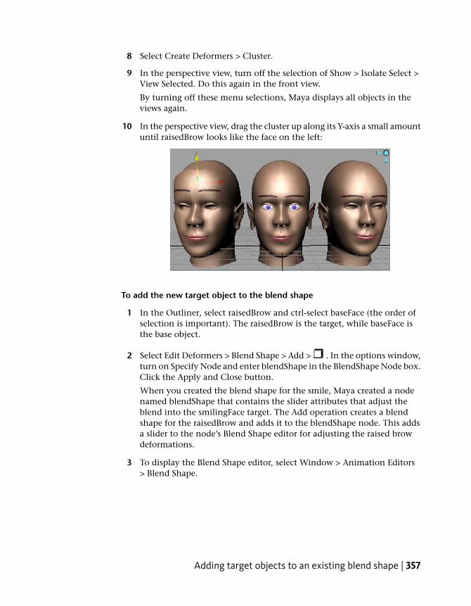
8 Select Create Deformers > Cluster.
9 In the perspective view, turn off the selection of Show > Isolate Select >View Selected. Do this again in the front view.
By turning off these menu selections, Maya displays all objects in theviews again.
10 In the perspective view, drag the cluster up along its Y-axis a small amountuntil raisedBrow looks like the face on the left:
To add the new target object to the blend shape
1 In the Outliner, select raisedBrow and ctrl-select baseFace (the order ofselection is important). The raisedBrow is the target, while baseFace isthe base object.
2 Select Edit Deformers > Blend Shape > Add > . In the options window,turn on Specify Node and enter blendShape in the BlendShape Node box.Click the Apply and Close button.
When you created the blend shape for the smile, Maya created a nodenamed blendShape that contains the slider attributes that adjust theblend into the smilingFace target. The Add operation creates a blendshape for the raisedBrow and adds it to the blendShape node. This addsa slider to the node’s Blend Shape editor for adjusting the raised browdeformations.
3 To display the Blend Shape editor, select Window > Animation Editors> Blend Shape.
Adding target objects to an existing blend shape | 357

4 You can use the sliders alone or in combination to create a smile withraised eyebrows, a frown with lowered eyebrows, and so on.
5 You can optionally select raisedBrow and edit the cluster weights to tunethe deformation of the eyebrow region as desired. See Editing clusterweights on page 348 for details. An example weighting follows:
358 | Chapter 7 Character Setup

TIP After you create a blend shape, you can optionally hide or delete a targetobject (in this lesson, smilingFace and raisedBrow). If you delete a target, youimprove Maya processing time but lose the capability to manipulate thecluster handle. For versatility, many animators hide the target rather thandelete it. Hiding the target is necessary when you render the scene. It is alsouseful when you want to unclutter the scene view.
Beyond the lessonIn this lesson, you learned how to:
■ Use two clusters and a blend shape deformer to manipulate facialexpressions.In professional productions, it’s common to create several more clusterswith a blend shape deformer for finer control of facial expressions. Forexample, you can create clusters for a number of mouth positions that youcan use to simulate the phonemes of speech.
When you used certain blend shape slider values, you may have noticedthat the face looked good in all regions except for a few vertices. To fixsuch regions, delete the cluster, move the problem vertices of the targetface to a better position, then create a blend shape for the improved targetface.
As much as possible, use a target shape that’s not extremely different fromthe base shape. If you need to use an extremely different target shape,create a blend shape with multiple targets. Each of the multiple targetsmust have a shape that is progressively more like the extreme target shape.
Beyond the lesson | 359
Before you create the blend shape, turn on In-Between in the Create BlendShape options window, and select the multiple targets in this order: leastextreme shape difference first, most extreme shape difference last.
Although the lesson showed how to blend individual objects, you can alsoblend hierarchies of objects. See the Maya Help for more information.
There are some additional notes on clusters which are not explained in thislesson:
■ You can add or remove vertices from a cluster with Edit Deformers > PaintSet Membership Tool.
■ You can use the Component Editor to edit weight values more preciselythan by painting.
■ Avoid changing the number of vertices (or CVs) for a surface after youapply a cluster or other deformer. Unexpected deformations may occur.
360 | Chapter 7 Character Setup

Polygon Texturing
Introduction
Texture maps let you modify the appearance of your 3D models and scenes inMaya. Texture maps are images you apply and accurately position onto yoursurfaces using a process called texture mapping. When an image is texture mappedonto a surface, it alters the appearance of the surface in some unique way.Texture maps let you create many interesting visual effects:
■ You can apply labels and logos to your surfaces.
■ You can apply surface relief details and features to a surface instead of havingto model the details on the surface directly.
■ You can use illustrations as texture maps to create interesting backdrops inyour scenes.
8
361
Most shading attributes for a surface material can be altered by a texture map.For example, color, specular, transparency, and reflectivity are examples ofattributes that can be modified by a texture map.
Texture mapping is a key component in the 3D production workflow. Manyproduction environments employ texture artists whose only role is to createand apply the texture maps to 3D models.
Preparing for the lessonTo ensure the lesson works as described, do these steps before beginning:
1 Select File > New Scene to create a new scene.
2 Make sure the Construction History icon (below the menu bar) is on:
(If it is turned off, it has a large X across it.)
3 If you have not already done so, copy the GettingStarted folder fromits installation location to your projects directory. Then, set theGettingStarted directory as your Maya project. For more information,see Copying and setting the Maya project on page 25.
4 Select the Polygons menu set. Unless otherwise noted, the directions inthis chapter for making menu selections assume you’ve already selectedthe Polygons menu set.
5 Make sure Display > UI Elements > Help Line is turned on. You will usethe Help Line while modeling.
6 Ensure that the interactive creation option for primitives is turned off byselecting Create > Polygon Primitives > Interactive Creation. The optionis off when a check mark does not display beside the item’s name in themenu.
7 Make sure that Soft Selection is turned off by opening the Attribute Editorwith the Select Tool active and unchecking the box marked Soft Select.
362 | Chapter 8 Polygon Texturing
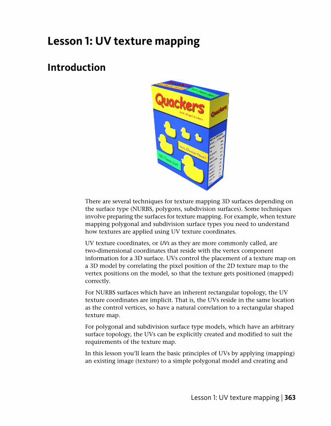
Lesson 1: UV texture mapping
Introduction
There are several techniques for texture mapping 3D surfaces depending onthe surface type (NURBS, polygons, subdivision surfaces). Some techniquesinvolve preparing the surfaces for texture mapping. For example, when texturemapping polygonal and subdivision surface types you need to understandhow textures are applied using UV texture coordinates.
UV texture coordinates, or UVs as they are more commonly called, aretwo-dimensional coordinates that reside with the vertex componentinformation for a 3D surface. UVs control the placement of a texture map ona 3D model by correlating the pixel position of the 2D texture map to thevertex positions on the model, so that the texture gets positioned (mapped)correctly.
For NURBS surfaces which have an inherent rectangular topology, the UVtexture coordinates are implicit. That is, the UVs reside in the same locationas the control vertices, so have a natural correlation to a rectangular shapedtexture map.
For polygonal and subdivision surface type models, which have an arbitrarysurface topology, the UVs can be explicitly created and modified to suit therequirements of the texture map.
In this lesson you’ll learn the basic principles of UVs by applying (mapping)an existing image (texture) to a simple polygonal model and creating and
Lesson 1: UV texture mapping | 363

modifying the UV texture coordinates so that the texture map appears correctlyon the surface.
In this lesson you learn how to:
■ Assign a 2D texture map to a polygonal model.
■ Map UV texture coordinates (UVs) to a polygonal surface.
■ Correlate the UVs between the scene view and the UV Texture Editor.
■ Use the UV Texture Editor to visualize how the UV texture coordinatesfrom a three-dimensional model relate to an assigned two-dimensionaltexture map.
■ Determine basic UV layout requirements.
■ Set preferences to let you visualize the texture borders in both the UVTexture Editor and the scene view to better understand how the texturemap is placed on the polygonal model.
■ Select and reposition UV texture coordinates within the UV Texture Editorusing the transformation tools to make the UVs match a pre-defined texturemap.
■ Sew UV texture coordinates to existing UV shells.
Creating a cracker box modelYou begin the lesson by creating a model of a cracker box using a polygonalcube primitive. The dimensions you’ll use for the cracker box are based on atexture map you’ll apply to the model in this lesson.
To create a cracker box model using a cube primitive
1 Select Create > Polygon Primitives > Cube > .
2 In the Polygon Cube Options window, select Edit > Reset Settings, setthe following options, and then click Create:
■ Width: 8
■ Height: 10
■ Depth: 3
■ Width divisions: 1
364 | Chapter 8 Polygon Texturing
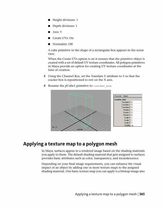
■ Height divisions: 1
■ Depth divisions: 1
■ Axis: Y
■ Create UVs: On
■ Normalize: Off
A cube primitive in the shape of a rectangular box appears in the sceneview.
When the Create UVs option is on it ensures that the primitive object iscreated with a set of default UV texture coordinates. All polygon primitivesin Maya provide an option for creating UV texture coordinates at thetime of creation.
3 Using the Channel Box, set the Translate Y attribute to 5 so that thecracker box is repositioned to rest on the X axis.
4 Rename the pCube1 primitive to: cracker_box.
Applying a texture map to a polygon meshIn Maya, surfaces appear in a rendered image based on the shading materialsyou apply to them. The default shading material that gets assigned to surfacesprovides basic attributes such as color, transparency, and incandescence.
Depending on your final image requirements, you can enhance the visualimpact of an object by adding one or more texture maps to the assignedshading material. One basic texture map you can apply is a bitmap image also
Applying a texture map to a polygon mesh | 365
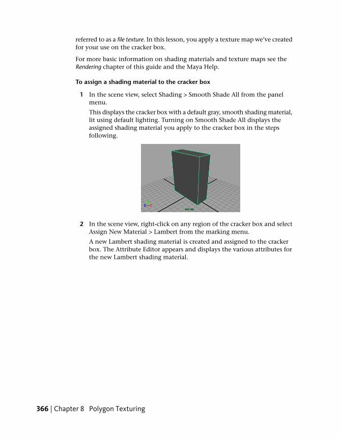
referred to as a file texture. In this lesson, you apply a texture map we’ve createdfor your use on the cracker box.
For more basic information on shading materials and texture maps see theRendering chapter of this guide and the Maya Help.
To assign a shading material to the cracker box
1 In the scene view, select Shading > Smooth Shade All from the panelmenu.
This displays the cracker box with a default gray, smooth shading material,lit using default lighting. Turning on Smooth Shade All displays theassigned shading material you apply to the cracker box in the stepsfollowing.
2 In the scene view, right-click on any region of the cracker box and selectAssign New Material > Lambert from the marking menu.
A new Lambert shading material is created and assigned to the crackerbox. The Attribute Editor appears and displays the various attributes forthe new Lambert shading material.
366 | Chapter 8 Polygon Texturing

The new Lambert material is identical to the default gray material thatwas previously assigned to the cracker box. However, it’s always a goodpractice not to modify the default shading material in the scene andcreate a new shading material and modify it to suit your requirements.
3 In Attribute Editor, double-click in the lambert2 box and then type:box_material to rename the shading material.
Renaming the shading material lets you easily identify it later on whenyou need to edit it. Naming items uniquely in Maya is a useful habit.
4 In the Attribute Editor, move the Color slider fully to the right so that thecolor box appears white.
The shading material assigned to the box model also updates in the sceneview so it appears in a brighter tone.
Applying a texture map to a polygon mesh | 367

5 Click the Map button located to the right of the Color slider.
The Create Render Node window appears and lists the various textureoptions you can apply (or connect) to the color channel of the boxmaterial.
6 Click PSD File from the list of 2D Textures.
Choosing this option specifies that you want to apply an Adobe®
Photoshop® format file as a texture. A PSD format file lets you keep thevarious components of your texture map on multiple layers. This is usefulwhen you need the ability to edit a component of the texture duringproduction.
The Attribute Editor updates to display the options for the PSD Filetexture.
TIP If the Attribute Editor suddenly appears empty, it indicates that no objectsare selected in the scene. Simply select the box model again in the scene todisplay the attributes for the box.
7 Click the Browse button (folder icon) to the right of the Image Nameattribute to specify the image file for the texture map.
368 | Chapter 8 Polygon Texturing

A browser window appears with the path set to the default projectdirectory. By default, Maya looks for source images for texture maps ina sourceimages folder whenever the project folder is set. Maya can usefile texture images from anywhere on your workstation or local network.For example, you can have images on a central disk drive that is sharedamong users in a production environment.
8 Select the image file named UVLesson.psd.
This file can be found in the GettingStarted directory that you set asyour Maya project:
GettingStarted/UVMapping/sourceimages
The image contains 2D artwork for the front, back, top, bottom, and sidesof the cracker box that was generated in Adobe® Photoshop®.
Applying a texture map to a polygon mesh | 369
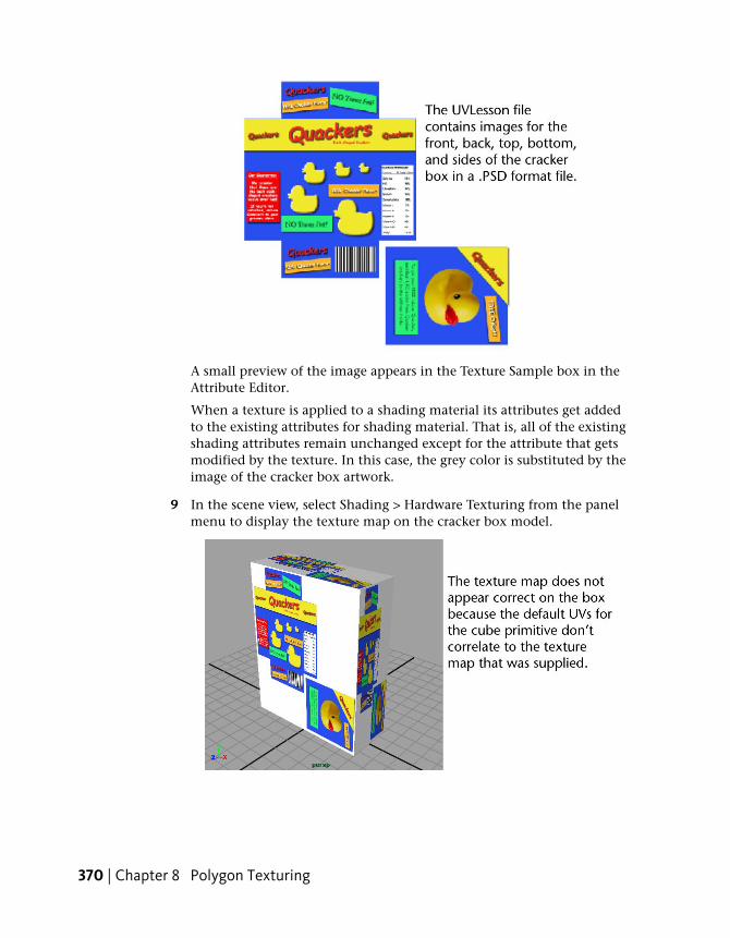
A small preview of the image appears in the Texture Sample box in theAttribute Editor.
When a texture is applied to a shading material its attributes get addedto the existing attributes for shading material. That is, all of the existingshading attributes remain unchanged except for the attribute that getsmodified by the texture. In this case, the grey color is substituted by theimage of the cracker box artwork.
9 In the scene view, select Shading > Hardware Texturing from the panelmenu to display the texture map on the cracker box model.
370 | Chapter 8 Polygon Texturing

The texture map does not appear correctly on the cracker box model.The texture map was designed so that specific sides of the box receivespecific regions of the image. Instead, the complete image is being placedon every side of the object.
To correct this problem you must modify the default UV texturecoordinates for the model so they match the layout of the texture image.To do this, you use the UV Texture Editor.
Viewing UVs in the UV Texture EditorThe UV Texture Editor lets you view and interactively edit the UV texturecoordinates for polygon and subdivision surface types. UVs appear laid flatwithin the UV Texture Editor’s 2D view. It also lets you display the 2D imagefor the texture map in relation to the UVs. These features are critical foraccurate and efficient placement of texture maps on polygon and subdivisionsurface types.
In this lesson, your goal is to ensure that the shape and placement of the UVsmatch the image as it appears in the 2D view of the UV Texture Editor. Thiswill ensure that the map appears correctly on the cracker box model in the3D scene view.
To open the UV Texture Editor in a two pane layout
➤ In the scene view, right-click any of the Quick Layout buttons on theToolbox to display the pop-up menu of Quick Layout shortcuts and selectPersp/UV Texture Editor from the list.
Viewing UVs in the UV Texture Editor | 371
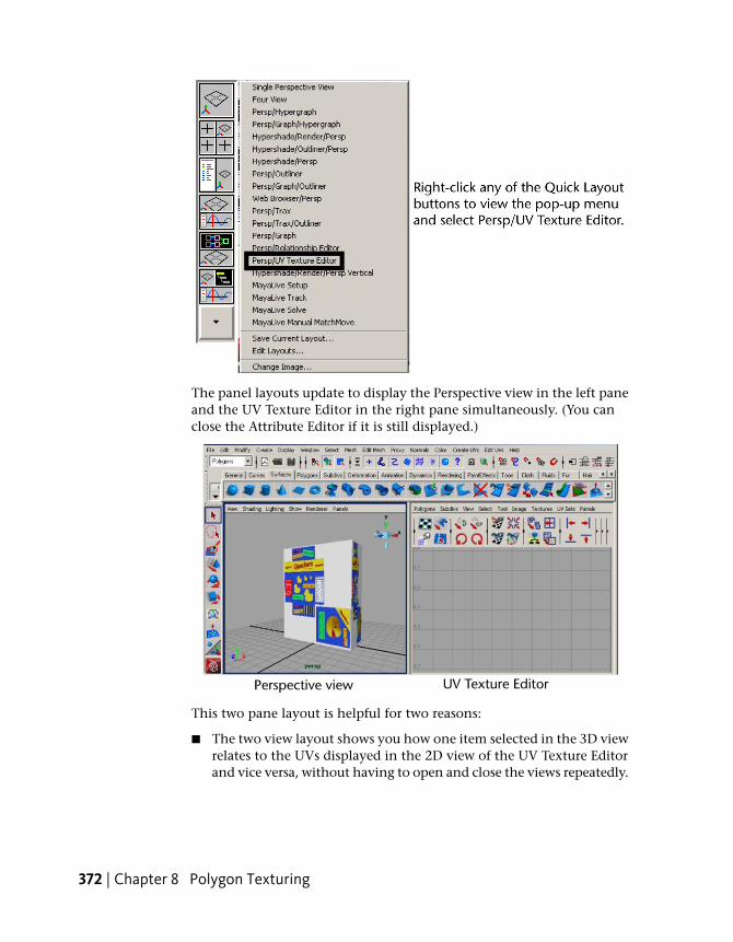
The panel layouts update to display the Perspective view in the left paneand the UV Texture Editor in the right pane simultaneously. (You canclose the Attribute Editor if it is still displayed.)
This two pane layout is helpful for two reasons:
■ The two view layout shows you how one item selected in the 3D viewrelates to the UVs displayed in the 2D view of the UV Texture Editorand vice versa, without having to open and close the views repeatedly.
372 | Chapter 8 Polygon Texturing

■ When you edit UVs for a surface mesh in the UV Texture Editor, youcan immediately see the effect of the texture map on the model inthe 3D scene view.
UVs do not initially appear in the 2D view of the UV Texture Editor until youselect an object or change the selection mode for an object in the scene view.
To view UVs in the UV Texture Editor
1 In the scene view, right-click any region of the cracker box model andselect Object Mode from the marking menu.
2 Select the cracker box model.
3 In the UV Texture Editor, dolly the view outwards so you can see the UVsfor the cracker box as shown below. (To dolly, press the Alt key and dragthe mouse to the left while holding down the right button on yourmouse.)
The UV texture coordinates for the cracker box model appear in the 2Dview of the UV Texture Editor as a flattened, two-dimensionalrepresentation. The UVs appear highlighted with lines connecting theUVs to indicate the region of the texture the UVs represent.
The image you specified as the texture map for the box also appears inthe 2D view of the UV Texture Editor in the upper right quadrant of the2D cartesian graph called the UV image range or UV Texture Space. Thecoordinates for this quadrant range from 0,0 to 1,1 and represent thetexture space for the surface. How the UVs appear in this quadrant in
Viewing UVs in the UV Texture Editor | 373
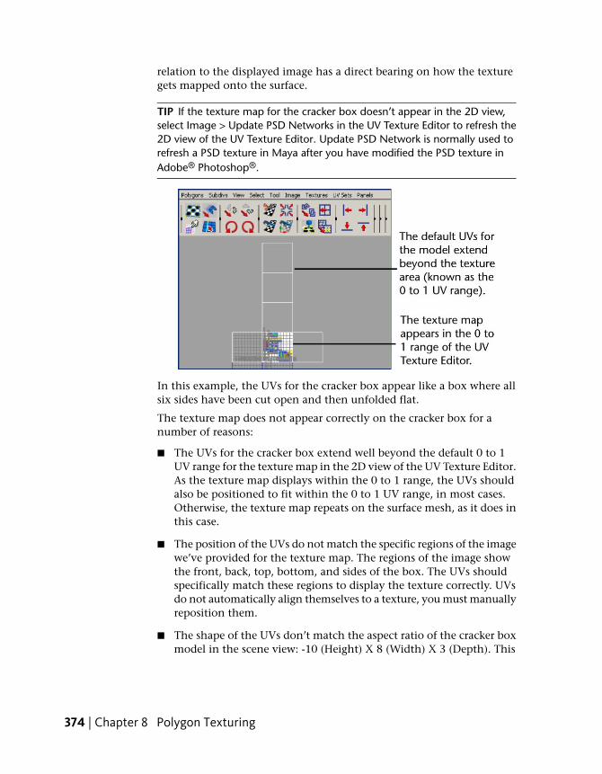
relation to the displayed image has a direct bearing on how the texturegets mapped onto the surface.
TIP If the texture map for the cracker box doesn’t appear in the 2D view,select Image > Update PSD Networks in the UV Texture Editor to refresh the2D view of the UV Texture Editor. Update PSD Network is normally used torefresh a PSD texture in Maya after you have modified the PSD texture inAdobe® Photoshop®.
In this example, the UVs for the cracker box appear like a box where allsix sides have been cut open and then unfolded flat.
The texture map does not appear correctly on the cracker box for anumber of reasons:
■ The UVs for the cracker box extend well beyond the default 0 to 1UV range for the texture map in the 2D view of the UV Texture Editor.As the texture map displays within the 0 to 1 range, the UVs shouldalso be positioned to fit within the 0 to 1 UV range, in most cases.Otherwise, the texture map repeats on the surface mesh, as it does inthis case.
■ The position of the UVs do not match the specific regions of the imagewe’ve provided for the texture map. The regions of the image showthe front, back, top, bottom, and sides of the box. The UVs shouldspecifically match these regions to display the texture correctly. UVsdo not automatically align themselves to a texture, you must manuallyreposition them.
■ The shape of the UVs don’t match the aspect ratio of the cracker boxmodel in the scene view: -10 (Height) X 8 (Width) X 3 (Depth). This
374 | Chapter 8 Polygon Texturing
is because the default UVs for a Maya cube primitive are created basedon a predetermined default shape and do not get updated if the shapeor scale of the primitive is modified later on.
There are a number of things you can do to correct these issues depending onthe situation. For this lesson, you will correct the UV and texture mapmisalignment by doing the following:
■ Map a new set of UVs for the cracker box model that better matches theindividual faces of the cracker box. (While the existing UVs could bemodified, you’ll learn how to create new UVs in this lesson that will bettermatch the size and scale of the 3D model.
■ Ensure the new UVs fit within the 0 to 1 UV range in the UV TextureEditor.
■ Reposition the UVs so that they correlate to specific locations on the 2Dimage using the UV Texture Editor. This will ensure that the various sidesof the box receive the correct regions of the texture map.
Mapping UV texture coordinatesIt is often necessary to create new UVs for a surface mesh in order to texturemap it correctly. These situations include:
■ Texture mapping a surface that doesn’t have existing UVs.This can occur when you import 3D models from other softwareapplications that don’t create UVs.
■ When the UVs for a surface are badly jumbled or are missing some UVs.This can occur when a surface has been edited or modified in some wayand it becomes hard to determine what UVs may be missing as a result.
■ When you need a unique set of UVs for a particular purpose.For example, if you want to paint a texture map directly onto a 3D surface,you may want to map UVs that allow you to paint using the 3D paint toolsin Maya. Alternatively, you may want to create a unique set of UVsspecifically for baking textures or light maps.
Maya lets you create UVs for polygonal and subdivision surfaces using a processcalled projection mapping, also referred to as mapping UVs. Maya provides severalprojection mapping types that map what gets viewed by a particular projection
Mapping UV texture coordinates | 375
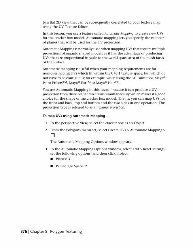
to a flat 2D view that can be subsequently correlated to your texture mapusing the UV Texture Editor.
In this lesson, you use a feature called Automatic Mapping to create new UVsfor the cracker box model. Automatic mapping lets you specify the numberof planes that will be used for the UV projection.
Automatic Mapping is normally used when mapping UVs that require multipleprojections of organic shaped models as it has the advantage of producingUVs that are proportional in scale to the world space area of the mesh facesof the surface.
Automatic mapping is useful when your mapping requirements are fornon-overlapping UVs which fit within the 0 to 1 texture space, but which donot have to be contiguous; for example, when using the 3D Paint tool, Maya®
Paint EffectsTM, Maya® FurTM or Maya® HairTM.
You use Automatic Mapping in this lesson because it can produce a UVprojection from three planar directions simultaneously which makes it a goodchoice for the shape of the cracker box model. That is, you can map UVs forthe front and back, top and bottom and the two sides in one operation. Thisprojection type is referred to as a triplanar projection.
To map UVs using Automatic Mapping
1 In the perspective view, select the cracker box as an Object.
2 From the Polygons menu set, select Create UVs > Automatic Mapping >
.
The Automatic Mapping Options window appears.
3 In the Automatic Mapping Options window, select Edit > Reset settings,set the following options, and then click Project:
■ Planes: 3
■ Percentage Space: 2
376 | Chapter 8 Polygon Texturing
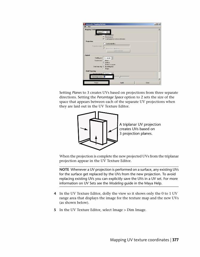
Setting Planes to 3 creates UVs based on projections from three separatedirections. Setting the Percentage Space option to 2 sets the size of thespace that appears between each of the separate UV projections whenthey are laid out in the UV Texture Editor.
When the projection is complete the new projected UVs from the triplanarprojection appear in the UV Texture Editor.
NOTE Whenever a UV projection is performed on a surface, any existing UVsfor the surface get replaced by the UVs from the new projection. To avoidreplacing existing UVs you can explicitly save the UVs in a UV set. For moreinformation on UV Sets see the Modeling guide in the Maya Help.
4 In the UV Texture Editor, dolly the view so it shows only the 0 to 1 UVrange area that displays the image for the texture map and the new UVs(as shown below).
5 In the UV Texture Editor, select Image > Dim Image.
Mapping UV texture coordinates | 377
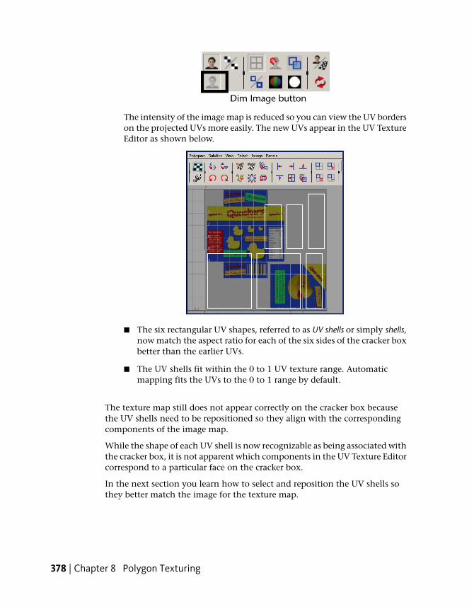
The intensity of the image map is reduced so you can view the UV borderson the projected UVs more easily. The new UVs appear in the UV TextureEditor as shown below.
■ The six rectangular UV shapes, referred to as UV shells or simply shells,now match the aspect ratio for each of the six sides of the cracker boxbetter than the earlier UVs.
■ The UV shells fit within the 0 to 1 UV texture range. Automaticmapping fits the UVs to the 0 to 1 range by default.
The texture map still does not appear correctly on the cracker box becausethe UV shells need to be repositioned so they align with the correspondingcomponents of the image map.
While the shape of each UV shell is now recognizable as being associated withthe cracker box, it is not apparent which components in the UV Texture Editorcorrespond to a particular face on the cracker box.
In the next section you learn how to select and reposition the UV shells sothey better match the image for the texture map.
378 | Chapter 8 Polygon Texturing

Working with UVs in the UV Texture EditorWhen texture mapping a polygon or subdivision surface type model it is oftennecessary to modify the UV components for a model so they match the texturemap. The UV Texture Editor provides many tools for working with UVs. Inthis section you learn how to:
■ Select UVs from either the scene view or the UV Texture Editor andaccurately correlate them. Selecting UV components is critical to modifyingthem accurately.
■ Sew UV shells together to reduce the number of UV components you needto work with.
■ Move and rotate UVs within the UV Texture Editor to make the UV shellsalign to the cracker box texture map.
Selecting UV components
You can select UV components from either the scene view or within the UVTexture Editor. Displaying both the 3D scene view and the 2D view of the UVTexture Editor lets you easily correlate which UV components are associatedwith a particular edge or vertex on the 3D model.
This is very helpful to understand the layout and orientation of your UVtexture coordinates in relation to the image used for a texture map and howthe map appears on the model in the 3D scene view.
To select UVs for a 3D model in the scene view
1 In the UV Texture Editor, select Image > Display Image to turn off thedisplay of the texture image.
Display Image works by turning the display of the assigned texture onor off in the 2D view of the UV Texture Editor. Turning the image offtemporarily aids in viewing only the UV components. This will be usefulin the steps that follow.
Working with UVs in the UV Texture Editor | 379
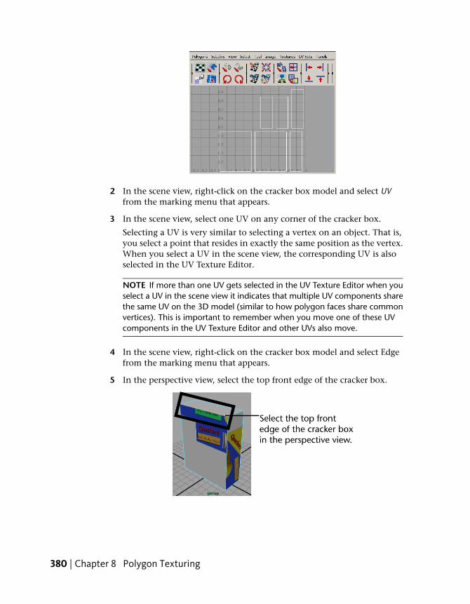
2 In the scene view, right-click on the cracker box model and select UVfrom the marking menu that appears.
3 In the scene view, select one UV on any corner of the cracker box.
Selecting a UV is very similar to selecting a vertex on an object. That is,you select a point that resides in exactly the same position as the vertex.When you select a UV in the scene view, the corresponding UV is alsoselected in the UV Texture Editor.
NOTE If more than one UV gets selected in the UV Texture Editor when youselect a UV in the scene view it indicates that multiple UV components sharethe same UV on the 3D model (similar to how polygon faces share commonvertices). This is important to remember when you move one of these UVcomponents in the UV Texture Editor and other UVs also move.
4 In the scene view, right-click on the cracker box model and select Edgefrom the marking menu that appears.
5 In the perspective view, select the top front edge of the cracker box.
380 | Chapter 8 Polygon Texturing

When you select this edge in the scene view, notice that twocorresponding shell edges also get selected in the UV Texture Editor. Thisindicates the following:
■ The selected edge is shared by two faces; the front and the top.
■ Selecting the top front edge in the scene view, identifies thecorresponding front and top UV shells for the box. (Indicated by theselection in the UV Texture Editor.)
This is useful when you need to understand how the various UV shellsrelate to each other, especially when you have many UV shells for a modelin the scene; for example, when you sew two UV shell edges together.
In the steps that follow you select edges in the UV Texture Editor so you cansew them together.
Sewing UVs
Sewing UV shells together merges the UV shells along a shared edge that youspecify. Sewing UVs is useful for the following reasons:
■ You can move and modify the UV shells as larger contiguous texture units.This makes it more efficient to match the UVs to the texture in manysituations.
■ Texture maps can appear more uniform across texture borders when thetexture is applied to one or more sewn UV shells compared to manyseparate UV shells. Sewing shells together reduces the chance that anunwanted texture mismatch occurs along the texture edge.
To sew shell edges together in the UV Texture Editor
1 In the scene view, ensure that only the top front edge of the cracker boxis still selected.
When the top front edge is selected in the scene view, the top edge ofone of the large UV shells is also selected as well as the left side of themiddle UV shell in the top row of the UV Texture Editor. For the crackerbox texture map, you need to sew these together so they correlate to themap correctly.
Working with UVs in the UV Texture Editor | 381

2 In the UV Texture Editor, select Polygons > Move and Sew UV Edges.
The small rectangular UV shell is repositioned to match the top of thelarge UV shell and the two shells are combined into one. When you laterselect and move this sewn shell, it will move as one piece. When two UVshells are selected for sewing, the smallest UV shell is moved to the larger.
3 Repeat steps 1 and 2 for the remaining three edges on front face of thecracker box keeping in mind the following:
■ Select only one edge at a time in the scene view.
■ When you’ve completed the move and sew operation, your UV TextureEditor should show the front UV shell with the corresponding top,bottom, and side shells sewn to it. When fully complete, you willhave only two UV shells to match to the texture image for the crackerbox.
382 | Chapter 8 Polygon Texturing

4 To display the texture borders for the two shells, select Texture BorderEdges. (You can also launch this window by right-clicking the ToggleTexture Borders button on the UV Texture Editor’s toolbar.)
In the UV Texture Editor, the texture borders for two UV shells nowappear with a thicker line.
Displaying texture borders on the UV shells is useful for visualizing where thetexture borders exist on the 3D model in the scene view. That is, any portionof the texture image that appears outside of the texture border will not appearon the surface. It is particularly useful for troubleshooting texture mismatcheswhen they occur. Displaying the texture borders can also help to identify
Working with UVs in the UV Texture Editor | 383

which UV shells are combined and which shells are not when you have manyUV shells displayed in the UV Texture Editor.
If you want to be able to view areas where UV shells overlap in the UV TextureEditor select Image > Shade UVs. When Shade UVs is turned on any selectedUV shells appear shaded in a semitransparent fashion. Areas where the shadingappears more opaque indicate the regions of shell overlap.
In the steps that follow, you reposition the two UV shells in the UV TextureEditor so they coincide with the texture image.
Moving UV components
You manually reposition UV components in the UV Texture Editor using thetools within the Toolbox. To reposition an individual UV component youmust first select it before selecting the Move Tool. To reposition an entire UVshell you must first select one individual UV from the shell it belongs to andthen convert the selection to a shell before using the Move Tool.
To move UVs in the UV Texture Editor
1 In the UV Texture Editor, select Image > Display Image.
The texture image displays in the 2D view of the UV Texture Editordimmed, as before. You need the image displayed so you can accuratelyreposition the two UV shells. Dimming the image aids in seeing theselected UVs.
2 In the UV Texture Editor, right-click and select UV from the markingmenu that appears.
3 In the UV Texture Editor, select one UV on the UV shell you sewed earlierin the lesson.
The UV coordinate appears highlighted in the 2D view.
4 Convert the selection to a UV shell by pressing the Ctrl key andright-clicking in the 2D view of the UV Texture Editor. Choose To Shellfrom the marking menu that appears.
The selection changes from a single selected UV to selecting the entireUV shell.
5 From the UV Texture Editor menu, select Tool > Move UV Shell Tool >
.
6 In the Move UV Shell Tool options window, turn off the Prevent overlapoption which prevents UV shells from being moved so they overlap andthen select Apply and Close.
384 | Chapter 8 Polygon Texturing
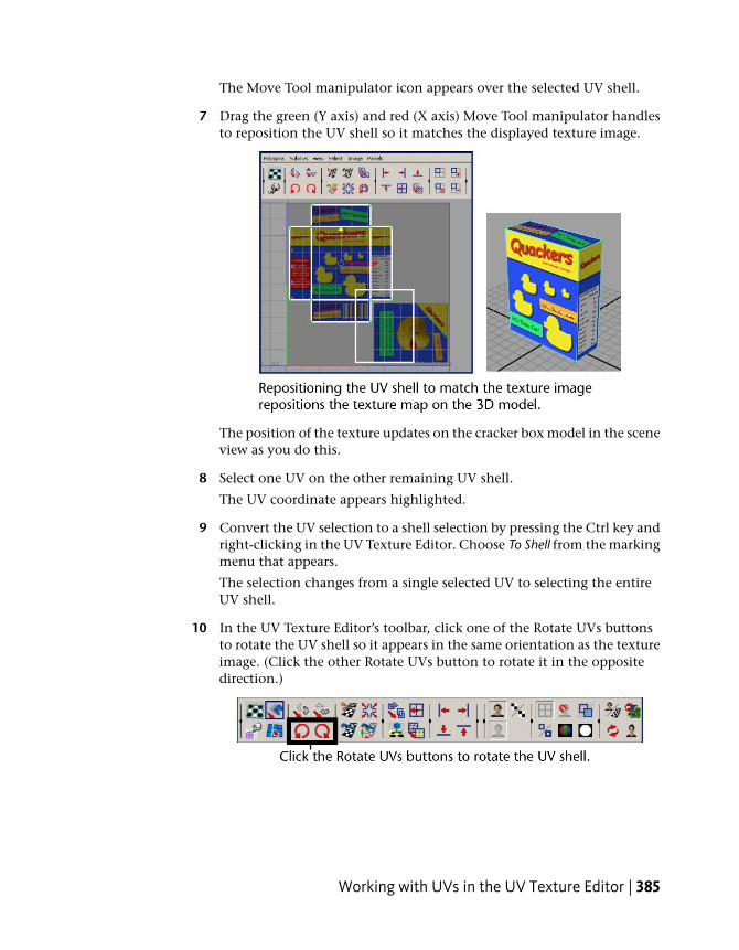
The Move Tool manipulator icon appears over the selected UV shell.
7 Drag the green (Y axis) and red (X axis) Move Tool manipulator handlesto reposition the UV shell so it matches the displayed texture image.
The position of the texture updates on the cracker box model in the sceneview as you do this.
8 Select one UV on the other remaining UV shell.
The UV coordinate appears highlighted.
9 Convert the UV selection to a shell selection by pressing the Ctrl key andright-clicking in the UV Texture Editor. Choose To Shell from the markingmenu that appears.
The selection changes from a single selected UV to selecting the entireUV shell.
10 In the UV Texture Editor’s toolbar, click one of the Rotate UVs buttonsto rotate the UV shell so it appears in the same orientation as the textureimage. (Click the other Rotate UVs button to rotate it in the oppositedirection.)
Working with UVs in the UV Texture Editor | 385

11 Confirm that the texture appears correctly on the cracker box model inthe scene view by tumbling the scene so you can view the back of thebox.
TIP If the texture appears upside down, you can continue to rotate it another180 degrees. If the texture appears reversed, that is, the letters are backwards,you can correct this by selecting Polygons > Flip from the UV Texture Editormenu and choosing the appropriate option setting.
12 From the UV Texture Editor menu, select Tool > Move UV Shell Tool.
A move manipulator icon appears over the selected UV shell.
13 Drag the green (Y axis) and red (X axis) manipulator handles to repositionthe UV shell so it matches the displayed texture image.
The texture map should now appear correct on all sides of the crackerbox when you’re finished.
TIP You can confirm that the UV shells are positioned accurately by dollyingin closer on the 2D view of the UV Texture Editor. If a minor correction isrequired, simply select and move the UVs or move the entire UV shell.
386 | Chapter 8 Polygon Texturing

TIP The exact UV boundaries can be viewed more clearly when theanti-aliasing for the texture image is temporarily turned off. To do this, selectImage > Display Unfiltered to view the texture image without anti-aliasing.
If you need to move a single UV so it precisely matches a particular locationon the texture map you can turn on Pixel Snap (Image > Pixel Snap). Whenyou select and move the UV using the Move Tool, it will reposition the UVcoordinate based on pixel boundaries.
Beyond the lessonIn this lesson you were introduced to a few of the basic techniques requiredto assign and accurately position texture maps on polygonal models using UVtexture coordinates:
■ UV coordinates are essential for applying and accurately positioning texturemaps on polygonal and subdivision surfaces.
■ UVs can be explicitly created for a surface mesh using a variety of UVmapping techniques. (Planar mapping, spherical mapping, cylindricalmapping, and Automatic mapping.)
■ UVs are represented as 2D coordinates and are viewed and edited withrespect to the 2D texture map using the UV Texture Editor. The UV TextureEditor provides many other tools for editing UVs.
■ UVs are usually positioned to fit within the 0 to 1 UV coordinate spaceunless the texture map requirements are such that the map needs to repeatacross the surface mesh.
■ It is useful to display both the 3D scene view and the 2D UV Texture Editorsimultaneously when texture mapping so that a correlation between the3D model and 2D UV coordinates can be made.
■ You can visualize texture borders using Texture Border Edges.
■ You can view the regions where UVs overlap each other in the UV TextureEditor by selecting the UV shells and selecting Image > Shade UVs.
You can open the PSD file you used in this lesson using Adobe® Photoshop®
to learn how layers were used for the texture map. You can edit one or moreof the layers to experiment with how the texture can be modified. After youmodify and save the file in Photoshop®, remember to select Image > Update
Beyond the lesson | 387

PSD Network in the UV Texture Editor so the texture map gets updated onthe model in the Maya scene.
If you would like to learn how to render an image of the cracker box modelsee the Rendering chapter of this guide as well as the Maya Help to learn moreabout lighting, shading, and rendering.
This lesson used a simple polygonal model to introduce the fundamentalconcepts. When you work with more complex polygonal and subdivisionsurface models, you can also:
■ layout overlapping UV shells that occur as a result of UV projectionmapping to ensure they fit within the 0 to 1 texture space using Edit UVs> Layout.
■ maximize the use of texture space by forcing the UV borders to be mappedto the full area of the 0 to 1 UV texture range using Edit UVs > Map UVBorder
■ align UVs to one another or snap them to the grid in the 2D view
■ untangle a UV mesh that contains overlapping UVs using Edit UVs > Relax.
■ modify a group of selected UVs using UV Lattice and UV Smudge tools
In general, you should begin texturing a model only after the model is fullycomplete. Otherwise, changes to the model may affect the associated UVtexture coordinates which in turn will affect how the texture appears on themodel.
In this lesson you matched the UVs to an existing texture image. Many textureartists create good UV layouts for their models prior to creating the actual 2Dimages for their texture maps. This is done only after the model is fullycomplete.
You can export a bitmap image of the 2D view of the UV Texture Editor touse as a guide for painting a texture in your favorite image creation software.In the UV Texture Editor, select Polygons > UV Snapshot to export the image.
If you use Adobe® Photoshop® for image creation and editing you can createa UV snapshot in a .PSD file format that creates the UV image on a separatelayer. To create the .PSD format file while working in the UV Texture Editor,select Image > Create PSD Network.
If you want to learn more about a particular tool or feature that was used inthis lesson, please refer to the Maya Help.
388 | Chapter 8 Polygon Texturing

Lesson 2: UV unfolding
Introduction
While texturing a flat object is fairly straightforward, texturing an object withcurves can pose some unique problems. How do you paint a 2D texture on acurved surface? How do you deal with a texture warping over bumps andgrooves? If you try to break apart the UV mesh like Lesson 1, you canpotentially end up with hundreds of small pieces.
To deal with these problems, artists typically use a workflow called unfoldingor pelting. Unfolding a UV mesh refers to the process of cutting a seam in theUV mesh (a mesh made up of UVs similar to how a polygon mesh is made ofvertices) and then unfolding along that seam. The process is similar to cuttinga seam along a shirt and laying it flat on a table. By laying out the UVs thisway, you can easily paint a texture on the 2D surface, which you can thenwrap around the model.
Lesson 2: UV unfolding | 389
In this lesson you learn how to:
■ Divide a mesh into separate parts for texturing.
■ Assign a basic checker pattern to judge the quality of a mapping.
■ Create a planar mapping.
■ Cut UV edges.
■ Unfold a UV mesh using the Unfold option.
■ Fix an unfolded mesh using the Smooth UVs tool.
Lesson SetupTo ensure the lesson works as described, do these steps before beginning:
■ Make sure you’ve done the steps in Preparing for the lesson on page 362.
■ Select the Polygons menu set by selecting it from the pull down menu onthe status line.
■ Open the scene file named Soldier.mb.This file can be found in the GettingStarted directory that you set as yourMaya project.
GettingStarted/UVMapping/Soldier.mb
The scene contains a polygon soldier.
■ In the panel menu, select Panels > Saved Layouts > Persp/UV Texture Editor.Your view is split between the perspective view and UV Texture Editor.
390 | Chapter 8 Polygon Texturing
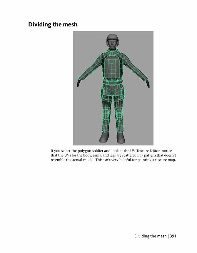
Dividing the mesh
If you select the polygon soldier and look at the UV Texture Editor, noticethat the UVs for the body, arms, and legs are scattered in a pattern that doesn’tresemble the actual model. This isn’t very helpful for painting a texture map.
Dividing the mesh | 391

To simplify the job, you need to divide the mesh into multiple pieces thatyou can then texture individually. Generally, you want to divide the meshinto pieces that can be unfolded into approximate square or rectangle shapes.This requires some pre-planning.
In this lesson you divide the body mesh into a torso, arms, and legs.
To divide the mesh into pieces
1 In the panel menu select Panels > Orthographic > front.
The perspective view changes to an orthographic front view of the soldier.
392 | Chapter 8 Polygon Texturing

2 Right-click the mesh and select Face from the marking menu.
3 Drag-select the faces on the right arm up to the shoulder.
4 Select Mesh > Extract.
Dividing the mesh | 393
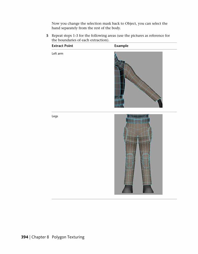
Now you change the selection mask back to Object, you can select thehand separately from the rest of the body.
5 Repeat steps 1-3 for the following areas (use the pictures as reference forthe boundaries of each extraction).
ExampleExtract Point
Left arm
Legs
394 | Chapter 8 Polygon Texturing

This leaves you with individual meshes for the arms, legs, and chest. The head,feet, and hands have already been done for you. This division allows you totexture each part individually.
Creating a planar mappingTo texture an organic object, you must start by creating a planar mapping asa base, which you can then unfold.
To create a planar map for the torso
1 Right-click the torso and select Object mode from the marking menu.
2 Select the torso.
3 Select Create UVs > Planar Mapping > .
The Planar Mapping Options window appears.
4 Select Edit > Reset Settings.
5 Set Project From to Z axis.
6 Click Project.
Creating a planar mapping | 395

Maya creates a new UV mapping for the torso. If you look at the UV TextureEditor, you can see the new UVs look like a flattened version of the front ofthe chest. At first glance this may seem perfect, but there’s a major problemhere that you need to change the UV Texture Editor view to shaded mode tosee.
To turn on shaded UV display
1 Select Window > UV Texture Editor.
The UV Texture Editor appears.
2 In the UV Texture Editor, click the Shade UVs icon ( ), or selectImage > Shade UVs.
In shaded UV mode, overlapping faces appear red while non-overlapping facesappear blue.
396 | Chapter 8 Polygon Texturing
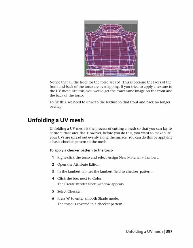
Notice that all the faces for the torso are red. This is because the faces of thefront and back of the torso are overlapping. If you tried to apply a texture tothe UV mesh like this, you would get the exact same image on the front andthe back of the torso.
To fix this, we need to unwrap the texture so that front and back no longeroverlap.
Unfolding a UV meshUnfolding a UV mesh is the process of cutting a mesh so that you can lay itsentire surface area flat. However, before you do this, you want to make sureyour UVs are spread out evenly along the surface. You can do this by applyinga basic checker pattern to the mesh.
To apply a checker pattern to the torso
1 Right-click the torso and select Assign New Material > Lambert.
2 Open the Attribute Editor.
3 In the lambert tab, set the lambert field to checker_pattern.
4 Click the box next to Color.
The Create Render Node window appears.
5 Select Checker.
6 Press ‘6’ to enter Smooth Shade mode.
The torso is covered in a checker pattern.
Unfolding a UV mesh | 397
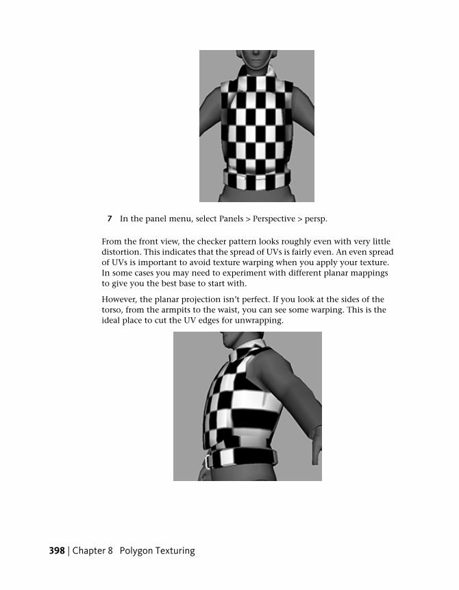
7 In the panel menu, select Panels > Perspective > persp.
From the front view, the checker pattern looks roughly even with very littledistortion. This indicates that the spread of UVs is fairly even. An even spreadof UVs is important to avoid texture warping when you apply your texture.In some cases you may need to experiment with different planar mappingsto give you the best base to start with.
However, the planar projection isn’t perfect. If you look at the sides of thetorso, from the armpits to the waist, you can see some warping. This is theideal place to cut the UV edges for unwrapping.
398 | Chapter 8 Polygon Texturing

To cut the UV edges
1 Right-click the vest and select Edge from the marking menu.
2 Select all the edges in a line that runs from under the arm, down the sideof the soldier’s body to the bottom of the vest. You can do this bydouble-clicking edges along this path until they are all selected.
3 Shift-select the corresponding edges on the other side.
An edge loop on both sides should be selected now.
4 In the UV Texture Editor, select Polygons > Cut UV Edges.
Now you are ready to unfold the mesh.
To unfold the torso
1 Right-click the torso and select UV.
2 Select one UV at the inside tip of each vest strap, along the unfold line.
Unfolding a UV mesh | 399
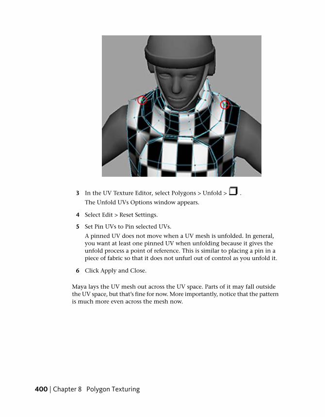
3 In the UV Texture Editor, select Polygons > Unfold > .
The Unfold UVs Options window appears.
4 Select Edit > Reset Settings.
5 Set Pin UVs to Pin selected UVs.
A pinned UV does not move when a UV mesh is unfolded. In general,you want at least one pinned UV when unfolding because it gives theunfold process a point of reference. This is similar to placing a pin in apiece of fabric so that it does not unfurl out of control as you unfold it.
6 Click Apply and Close.
Maya lays the UV mesh out across the UV space. Parts of it may fall outsidethe UV space, but that’s fine for now. More importantly, notice that the patternis much more even across the mesh now.
400 | Chapter 8 Polygon Texturing
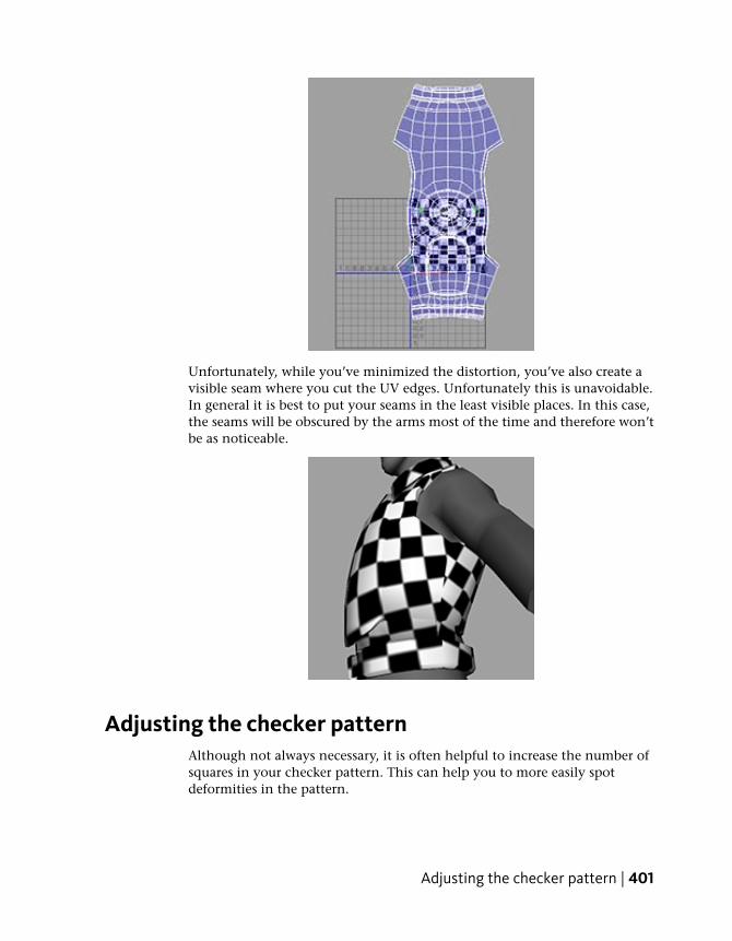
Unfortunately, while you’ve minimized the distortion, you’ve also create avisible seam where you cut the UV edges. Unfortunately this is unavoidable.In general it is best to put your seams in the least visible places. In this case,the seams will be obscured by the arms most of the time and therefore won’tbe as noticeable.
Adjusting the checker patternAlthough not always necessary, it is often helpful to increase the number ofsquares in your checker pattern. This can help you to more easily spotdeformities in the pattern.
Adjusting the checker pattern | 401
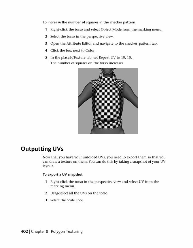
To increase the number of squares in the checker pattern
1 Right-click the torso and select Object Mode from the marking menu.
2 Select the torso in the perspective view.
3 Open the Attribute Editor and navigate to the checker_pattern tab.
4 Click the box next to Color.
5 In the place2dTexture tab, set Repeat UV to 10, 10.
The number of squares on the torso increases.
Outputting UVsNow that you have your unfolded UVs, you need to export them so that youcan draw a texture on them. You can do this by taking a snapshot of your UVlayout.
To export a UV snapshot
1 Right-click the torso in the perspective view and select UV from themarking menu.
2 Drag-select all the UVs on the torso.
3 Select the Scale Tool.
402 | Chapter 8 Polygon Texturing
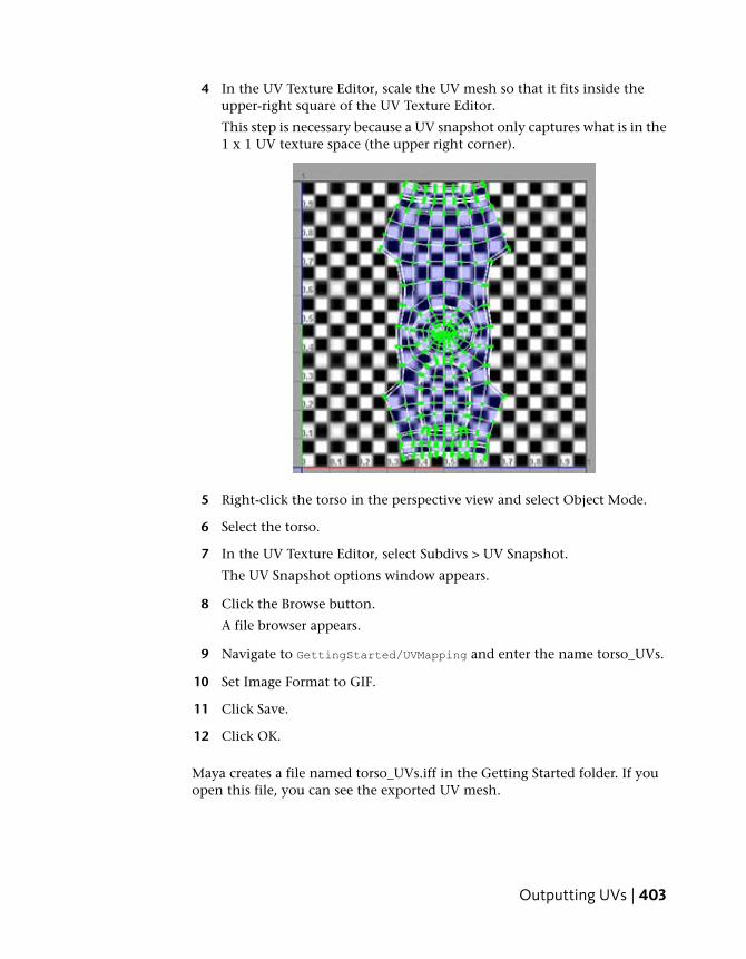
4 In the UV Texture Editor, scale the UV mesh so that it fits inside theupper-right square of the UV Texture Editor.
This step is necessary because a UV snapshot only captures what is in the1 x 1 UV texture space (the upper right corner).
5 Right-click the torso in the perspective view and select Object Mode.
6 Select the torso.
7 In the UV Texture Editor, select Subdivs > UV Snapshot.
The UV Snapshot options window appears.
8 Click the Browse button.
A file browser appears.
9 Navigate to GettingStarted/UVMapping and enter the name torso_UVs.
10 Set Image Format to GIF.
11 Click Save.
12 Click OK.
Maya creates a file named torso_UVs.iff in the Getting Started folder. If youopen this file, you can see the exported UV mesh.
Outputting UVs | 403

You can now open this file using an external image editor and paint yourtexture using the mesh as a guide.
NOTE If your image editing software does not support Maya .iff images, you canchange the image format in the UV Snapshot options window and then exportthe file again.
Unfolding with constraintsSometimes you only need to unfold a UV mesh in one direction. This isespecially useful when there is only a single seam.
To make things easier, you can use one of Maya’s Saved Layouts to keep boththe Perspective view and the UV Texture Editor in view simultaneously.
To view the perspective view and UV Texture Editor simultaneously
1 Close the UV Texture Editor window.
2 In the panel menu, select Panels > Saved Layouts > Persp/UV TextureEditor.
The perspective view and UV Texture Editor appear side-by-side in theviewport.
404 | Chapter 8 Polygon Texturing
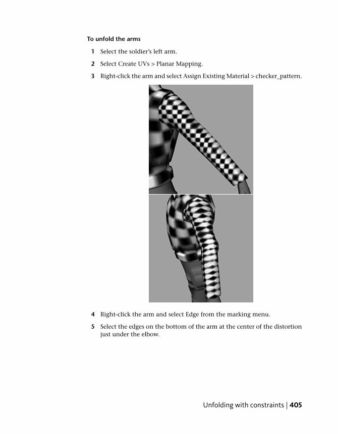
To unfold the arms
1 Select the soldier’s left arm.
2 Select Create UVs > Planar Mapping.
3 Right-click the arm and select Assign Existing Material > checker_pattern.
4 Right-click the arm and select Edge from the marking menu.
5 Select the edges on the bottom of the arm at the center of the distortionjust under the elbow.
Unfolding with constraints | 405

6 In the UV Texture Editor, select Polygons > Cut UVs.
7 Right-click the arm and select UV from the marking menu.
8 Drag-select all the UVs on the arm and click the Rotate clockwise button
( ).
The UVs rotate so the arm in the UV Texture Editor is vertical.
9 Select one UV at the top of the arm’s tricep and another UV at the tip ofthe soldier’s cuff.
406 | Chapter 8 Polygon Texturing

10 In the UV Texture Editor, select Polygons > Unfold > .
The Unfold UVs Options window appears.
11 Set Unfold constraint to Horizontal.
12 Click Apply and Close.
The UV mesh for the arm is unfolded evenly up and down. This is better thanthe UV mesh we would get if we unfolded in all directions.
Unfolding with constraints | 407
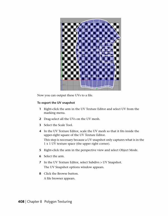
Now you can output these UVs to a file.
To export the UV snapshot
1 Right-click the arm in the UV Texture Editor and select UV from themarking menu.
2 Drag-select all the UVs on the UV mesh.
3 Select the Scale Tool.
4 In the UV Texture Editor, scale the UV mesh so that it fits inside theupper-right square of the UV Texture Editor.
This step is necessary because a UV snapshot only captures what is in the1 x 1 UV texture space (the upper right corner).
5 Right-click the arm in the perspective view and select Object Mode.
6 Select the arm.
7 In the UV Texture Editor, select Subdivs > UV Snapshot.
The UV Snapshot options window appears.
8 Click the Browse button.
A file browser appears.
408 | Chapter 8 Polygon Texturing

9 Navigate to GettingStarted/UVMapping and enter the name left_arm_UVs.
10 Set Image Format to GIF.
11 Click Save.
12 Click OK.
Like the torso you did in the previous step, Maya outputs a .gif filecontaining the UV mesh. You can import this file into an image editorand use it as a template to create a texture.
Now repeat the entire procedure for the right arm. Note that you do not needto output the UVs for the right arm because it will use the same texture as theleft arm.
Although you could handle the legs the same way you handled the arms(cutting them into two pieces), you can also treat the entire lower body as asingle mesh. You can follow the same procedure as above, except for thefollowing:
■ Select the edges down the rear until directly underneath the groin thenselect the edges on the inside of each leg. Cut these UV edges.
Unfolding with constraints | 409

■ You do not need to pin any UVs for the pants.
■ Like the arms, unfold the UV mesh horizontally.
410 | Chapter 8 Polygon Texturing

As with the torso and arms, you can now output these UV meshes to anexternal file to paint a texture on them. For information about how to do this,see Outputting UVs on page 402.
Sewing UV EdgesDepending on the mapping you start with, you may sometimes find that yourUV mesh is broken up in ways that can ruin your final result. In these cases,you can manually sew UV edges back together.
To map the head to the UV space
1 Select the head and select Create UVs > Cylindrical Mapping.
Sewing UV Edges | 411

2 Right-click the head and select Assign Existing Material > checker_pattern.
412 | Chapter 8 Polygon Texturing

Notice that because you started with a cylindrical mapping, the checkerpattern on the sides of the head aren’t warped like in the previousexamples. Unfortunately, if you tumble the camera you can see that thetop of the head is now warped. In this particular case this is preferableand you will see the reason why later.
If you turn on texture border display by clicking the texture border display
icon ( )in the UV Texture Editor, and re-examine the top of the helmet,you can see that a few edges that are not on the line of symmetry are coloredthick blue. This indicates that they are on the border of the UV mesh and willcause a seam. You can fix this by sewing these overlapping UV edges together.
To sew UV edges
1 Right-click the helmet and select Edge from the marking menu.
2 Shift-select the two thick blue edges at the top of the helmet that are noton the line of symmetry.
Sewing UV Edges | 413

3 In the UV Texture Editor, select Polygons > Sew UV Edges.
The thick blue edges change to match the other edges.
Notice that after sewing the UV edges together, the distortion has actuallygotten worse. However, this is only temporary and is fixed when you performthe unfold.
414 | Chapter 8 Polygon Texturing
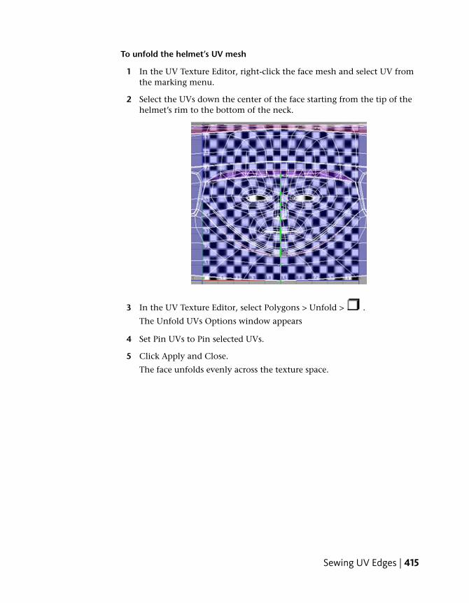
To unfold the helmet’s UV mesh
1 In the UV Texture Editor, right-click the face mesh and select UV fromthe marking menu.
2 Select the UVs down the center of the face starting from the tip of thehelmet’s rim to the bottom of the neck.
3 In the UV Texture Editor, select Polygons > Unfold > .
The Unfold UVs Options window appears
4 Set Pin UVs to Pin selected UVs.
5 Click Apply and Close.
The face unfolds evenly across the texture space.
Sewing UV Edges | 415
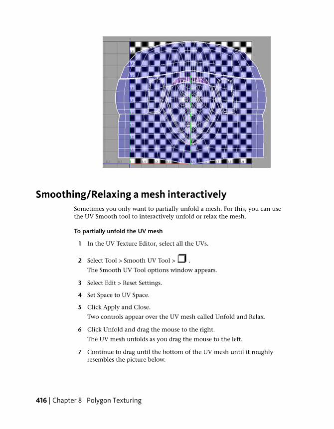
Smoothing/Relaxing a mesh interactivelySometimes you only want to partially unfold a mesh. For this, you can usethe UV Smooth tool to interactively unfold or relax the mesh.
To partially unfold the UV mesh
1 In the UV Texture Editor, select all the UVs.
2 Select Tool > Smooth UV Tool > .
The Smooth UV Tool options window appears.
3 Select Edit > Reset Settings.
4 Set Space to UV Space.
5 Click Apply and Close.
Two controls appear over the UV mesh called Unfold and Relax.
6 Click Unfold and drag the mouse to the right.
The UV mesh unfolds as you drag the mouse to the left.
7 Continue to drag until the bottom of the UV mesh until it roughlyresembles the picture below.
416 | Chapter 8 Polygon Texturing

If you reach the edge of the screen you can release the mouse button,click the Unfold control and drag again.
Fixing problem areasYou now have an unfolded UV mesh with no major overlapping faces.However, there are still a few minor problem areas where the mesh overlapsitself (particularly the eyes and mouth).
You can use the Smooth UV Tool to fix small imperfections in the shell withtargeted unfolds or relax operations.
To fix the eyes
1 In the perspective view, right-click the soldier’s head and select Edge fromthe marking menu.
2 Shift-select the four closest edge loops that surround each eye. You cando this quickly by Shift + double-clicking one edge in each loop.
Fixing problem areas | 417

3 In the UV Texture Editor, Ctrl + right-click the UV mesh and select ToUV from the marking menu.
The edges selected around the eyes are converted to the UVs selectedaround the eyes.
418 | Chapter 8 Polygon Texturing
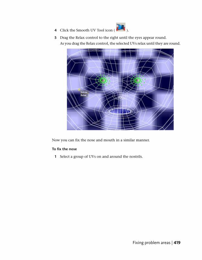
4 Click the Smooth UV Tool icon ( ).
5 Drag the Relax control to the right until the eyes appear round.
As you drag the Relax control, the selected UVs relax until they are round.
Now you can fix the nose and mouth in a similar manner.
To fix the nose
1 Select a group of UVs on and around the nostrils.
Fixing problem areas | 419

2 Drag the Relax control to the right until the UVs stop moving.
420 | Chapter 8 Polygon Texturing

To fix the mouth
1 In the perspective view, right-click the head and select Edge from themarking menu.
2 Shift-select the 4 edge loops around the mouth. You can do this quicklyby Shift + double-clicking one edge in each loop.
3 In the UV Texture Editor, Ctrl + right-click the UV mesh and select ToUV from the marking menu.
The edges selected around the mouth are converted to the UVs selectedaround the mouth.
Fixing problem areas | 421

4 Drag the Relax control to the right until the UVs stop moving.
The mouth UVs even out into a circular shape.
5 Select all the UVs on the head.
422 | Chapter 8 Polygon Texturing

6 Select the Scale Tool and scale the UVs so that they fit in the upper rightcorner of the UV space.
The UV mesh for the soldier’s head now has no UV faces overlapping. Thisallows you maximum control over what shows up in each portion of the headwhen you create the texture map for the soldier.
As with the rest of the body, you can now output these UV meshes to anexternal file to paint a texture on them. For information about how to do this,see Outputting UVs on page 402.
Applying TexturesNow that you’ve outputted all your UV meshes, you can import them intoan external image editor to create a texture.
Applying Textures | 423

Once you’ve created associated texture files, you need to apply them to yourmodel. For the purposes of this tutorial, textures have been provided for youin the sourceimages folder.
To apply the texture for the torso
1 In the perspective view, right-click the torso and select Assign NewMaterial > Lambert from the marking menu.
The soldier’s torso turns matte grey.
2 Open the Attribute Editor and select the lambert tab.
3 Change the name of the lambert material to Mat_Torso.
4 Click the box next to Color.
The Create Render Node window appears.
5 Click File.
6 Click the file icon next to the Image Name field.
A file browser appears.
7 Navigate to the Getting Started folder and selectUVMapping/sourceimages/soldier_torso.tif.
The body armor texture is applied to the soldier’s body. If the texture isnot aligned or sized correctly you can adjust the UVs in the UV TextureEditor using the Scale Tool in the Toolbox. If the texture does not appearin the scene, press ‘6’.
424 | Chapter 8 Polygon Texturing
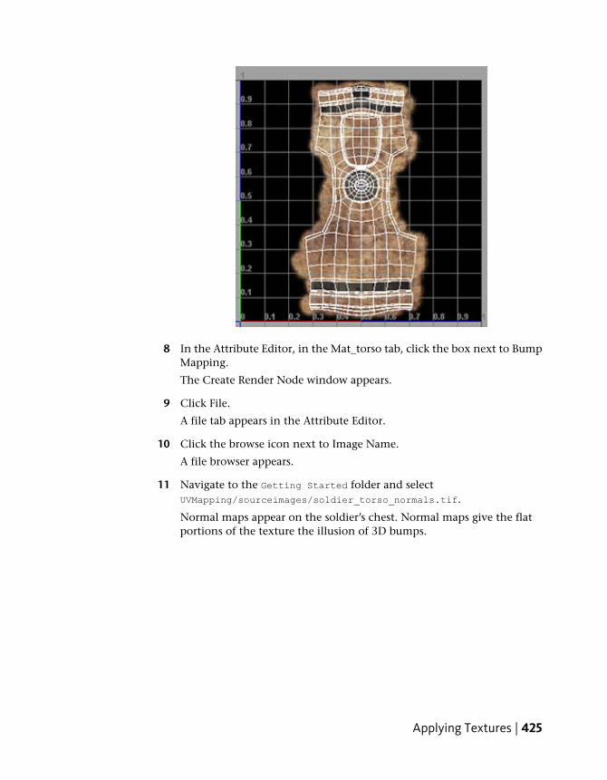
8 In the Attribute Editor, in the Mat_torso tab, click the box next to BumpMapping.
The Create Render Node window appears.
9 Click File.
A file tab appears in the Attribute Editor.
10 Click the browse icon next to Image Name.
A file browser appears.
11 Navigate to the Getting Started folder and selectUVMapping/sourceimages/soldier_torso_normals.tif.
Normal maps appear on the soldier’s chest. Normal maps give the flatportions of the texture the illusion of 3D bumps.
Applying Textures | 425
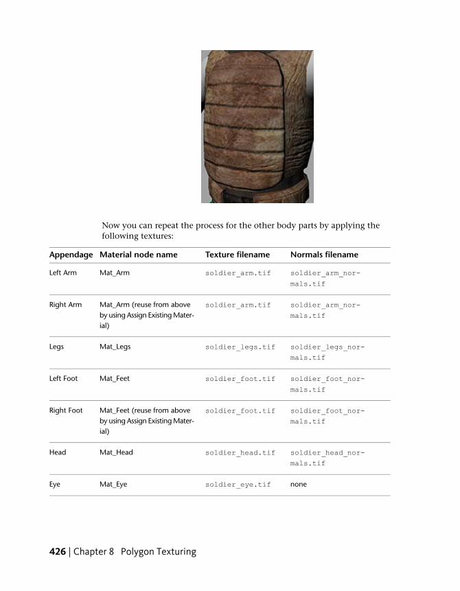
Now you can repeat the process for the other body parts by applying thefollowing textures:
Normals filenameTexture filenameMaterial node nameAppendage
soldier_arm_nor-
mals.tif
soldier_arm.tifMat_ArmLeft Arm
soldier_arm_nor-
mals.tif
soldier_arm.tifMat_Arm (reuse from aboveby using Assign Existing Mater-ial)
Right Arm
soldier_legs_nor-
mals.tif
soldier_legs.tifMat_LegsLegs
soldier_foot_nor-
mals.tif
soldier_foot.tifMat_FeetLeft Foot
soldier_foot_nor-
mals.tif
soldier_foot.tifMat_Feet (reuse from aboveby using Assign Existing Mater-ial)
Right Foot
soldier_head_nor-
mals.tif
soldier_head.tifMat_HeadHead
nonesoldier_eye.tifMat_EyeEye
426 | Chapter 8 Polygon Texturing
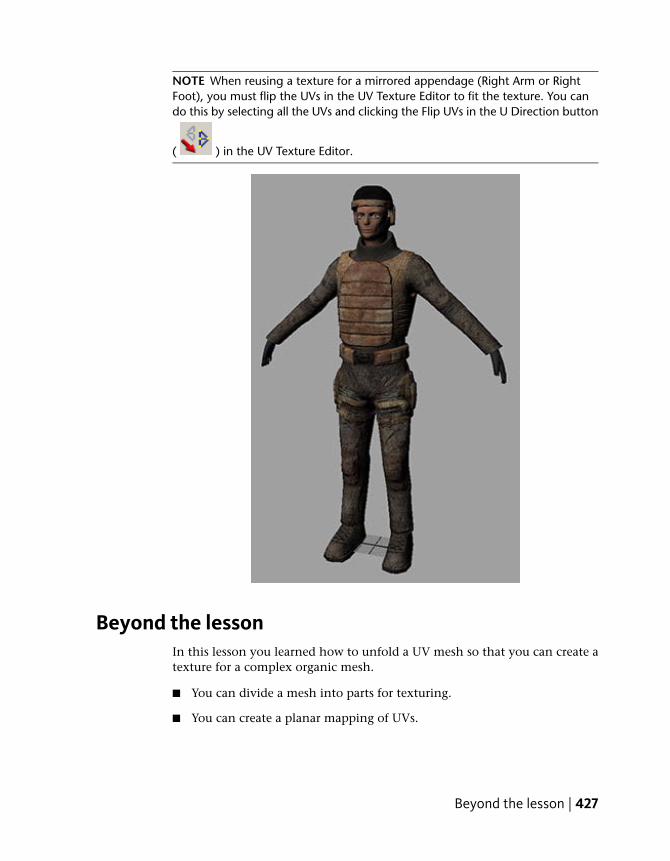
NOTE When reusing a texture for a mirrored appendage (Right Arm or RightFoot), you must flip the UVs in the UV Texture Editor to fit the texture. You cando this by selecting all the UVs and clicking the Flip UVs in the U Direction button
( ) in the UV Texture Editor.
Beyond the lessonIn this lesson you learned how to unfold a UV mesh so that you can create atexture for a complex organic mesh.
■ You can divide a mesh into parts for texturing.
■ You can create a planar mapping of UVs.
Beyond the lesson | 427

■ You can apply a basic checker texture to find problem areas.
■ You can cut UV edges in obscure areas to create a seam for unfolding.
■ You can pin a UV and unfold a mesh in all directions or constrained to asingle direction.
■ You can partially unfold a UV mesh with the UV Smooth Tool.
■ You can relax UVs to fix problem areas.
Lesson 3: Normal mapping
Introduction
Normal mapping is a technique in which you use a high resolution mesh togenerate a map for a low resolution mesh. High resolution meshes are madeup of more geometry and can be very taxing in an environment whereresources are at a premium (for example, in a large scene with other high polyobjects, or on a system with limited processing power). As a result, performancecan suffer greatly. Normal mapping is commonly used in these situations tocapture the detail of a high resolution mesh with the geometry of a lowresolution model.
428 | Chapter 8 Polygon Texturing
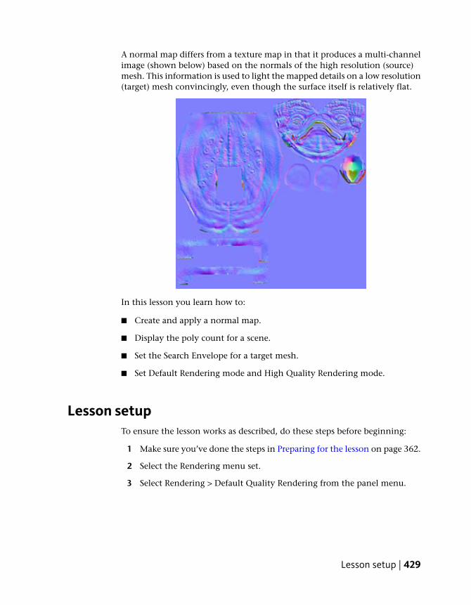
A normal map differs from a texture map in that it produces a multi-channelimage (shown below) based on the normals of the high resolution (source)mesh. This information is used to light the mapped details on a low resolution(target) mesh convincingly, even though the surface itself is relatively flat.
In this lesson you learn how to:
■ Create and apply a normal map.
■ Display the poly count for a scene.
■ Set the Search Envelope for a target mesh.
■ Set Default Rendering mode and High Quality Rendering mode.
Lesson setupTo ensure the lesson works as described, do these steps before beginning:
1 Make sure you’ve done the steps in Preparing for the lesson on page 362.
2 Select the Rendering menu set.
3 Select Rendering > Default Quality Rendering from the panel menu.
Lesson setup | 429
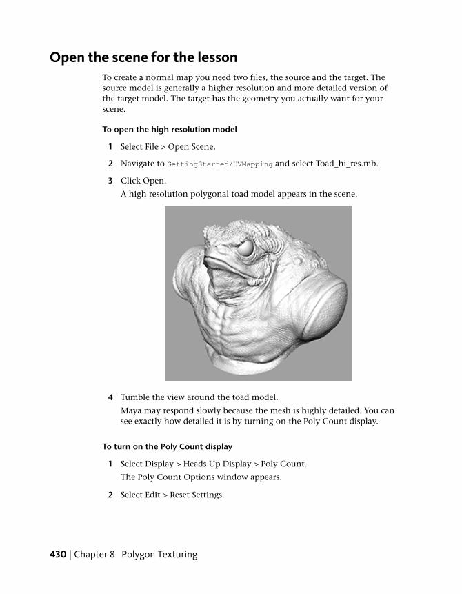
Open the scene for the lessonTo create a normal map you need two files, the source and the target. Thesource model is generally a higher resolution and more detailed version ofthe target model. The target has the geometry you actually want for yourscene.
To open the high resolution model
1 Select File > Open Scene.
2 Navigate to GettingStarted/UVMapping and select Toad_hi_res.mb.
3 Click Open.
A high resolution polygonal toad model appears in the scene.
4 Tumble the view around the toad model.
Maya may respond slowly because the mesh is highly detailed. You cansee exactly how detailed it is by turning on the Poly Count display.
To turn on the Poly Count display
1 Select Display > Heads Up Display > Poly Count.
The Poly Count Options window appears.
2 Select Edit > Reset Settings.
430 | Chapter 8 Polygon Texturing
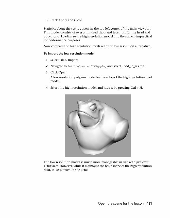
3 Click Apply and Close.
Statistics about the scene appear in the top left corner of the main viewport.This model consists of over a hundred thousand faces just for the head andupper torso. Loading such a high resolution model into the scene is impracticalfor performance purposes.
Now compare the high resolution mesh with the low resolution alternative.
To import the low resolution model
1 Select File > Import.
2 Navigate to GettingStarted/UVMapping and select Toad_lo_res.mb.
3 Click Open.
A low resolution polygon model loads on top of the high resolution toadmodel.
4 Select the high resolution model and hide it by pressing Ctrl + H.
The low resolution model is much more manageable in size with just over1500 faces. However, while it maintains the basic shape of the high resolutiontoad, it lacks much of the detail.
Open the scene for the lesson | 431
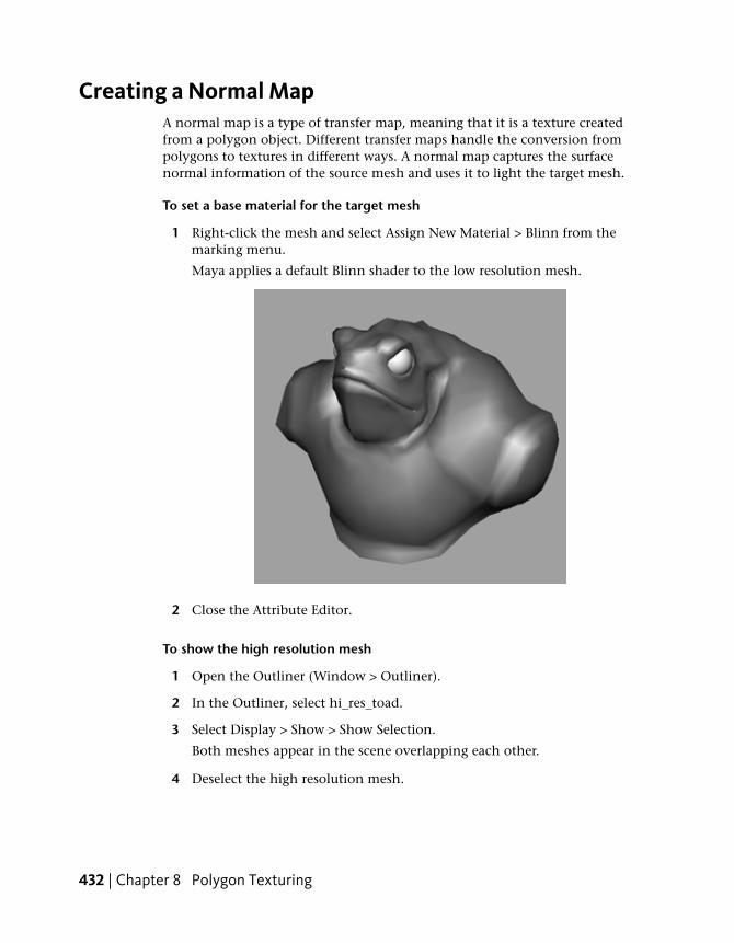
Creating a Normal MapA normal map is a type of transfer map, meaning that it is a texture createdfrom a polygon object. Different transfer maps handle the conversion frompolygons to textures in different ways. A normal map captures the surfacenormal information of the source mesh and uses it to light the target mesh.
To set a base material for the target mesh
1 Right-click the mesh and select Assign New Material > Blinn from themarking menu.
Maya applies a default Blinn shader to the low resolution mesh.
2 Close the Attribute Editor.
To show the high resolution mesh
1 Open the Outliner (Window > Outliner).
2 In the Outliner, select hi_res_toad.
3 Select Display > Show > Show Selection.
Both meshes appear in the scene overlapping each other.
4 Deselect the high resolution mesh.
432 | Chapter 8 Polygon Texturing

To create a normal map
1 Select Lighting/Shading > Transfer Maps.
The Transfer Maps window appears.
The Transfer Maps window lets you create various textures based onmappings from polygon models. First you need to assign the source andtarget meshes for the transfer.
2 In the Outliner, select lo_res_toad.
3 In the Transfer Maps window, in the Target Meshes section, click AddSelected.
4 In the Outliner, select hi_res_toad.
5 In the Transfer Maps window, in the Source Meshes section, click AddSelected.
Next you need to set the Search Envelope.
The Search Envelope represents the volume of the target geometry to considerfor the texture. Whatever part of the source mesh between the Search Envelopeand the target mesh is mapped to a texture.
Generally you want the Search Envelope to encompass your entire sourcemesh so you don’t miss any detail.
To set the Search Envelope
1 In the Transfer Maps window, set Display to Envelope.
The low resolution toad is replaced by a translucent red mesh.
This red mesh represents the Search Envelope.
2 Drag the slider under Search envelope (%) to the right.
The red mesh grows.
Drag the slider so that the red mesh barely encompasses all of the highresolution mesh without leaving any white spots (excluding the eyes).You can also enter a value in the box next to the slider. In this case, avalue of 4.3 yields just enough coverage around the two meshes.
Creating a Normal Map | 433

3 Set Display back to Mesh.
Now you can set the normal map options.
To set the normal map options
1 In the Transfer Maps window, under Output Maps, click Normal.
2 In the Normal Map text field, click the browse icon ( ).
A file browser appears.
3 Navigate to Getting Started/UVMapping and enter the name toad_texture.
4 Click Save.
5 Set File Format to DDS (dds).
434 | Chapter 8 Polygon Texturing

6 In the Transfer Maps window, set the following:
■ Under Connect Output Maps, set Connect maps to to Assigned shader.
■ Under Maya Common Output, set Map width and Map height to1024 and Sampling quality to Medium (4x4).
7 Click Bake and Close.
Maya generates a normal map.
NOTE It may take a few minutes for Maya to generate the normal map.
Viewing a normal mapNow that Maya has generated the normal map, you need to change the rendermode to High Quality Rendering mode to see it.
To view the normal mapped texture
1 Select the high resolution toad model hide it by pressing Ctrl +H.
2 In the panel menu, select Renderer > High Quality Rendering.
Now you can see the low resolution model with the detail of the highresolution model applied as a texture.
3 Tumble the view around the toad.
The light on the surface reacts appropriately to all the details on thetexture, without any loss in performance.
Viewing a normal map | 435

Beyond the lessonIn this lesson you learned how to use a high resolution model to create anormal map for a low resolution model. You learned how to:
■ Display the poly count for a scene.
■ Set the source and target for a normal map.
■ Set the Search Envelope.
■ Switch between Default Quality Rendering and High Quality Rendering.
You can also try applying other types of transfer maps to a low polygon model.Each mapping feature gives you slightly different looks on your low polygonmodel. For more information about transfer maps, see Lighting/Shading >Transfer Maps.
436 | Chapter 8 Polygon Texturing

Rendering
Introduction
In Maya, rendering refers to the process of creating bitmap images of your scenebased on the various shading, lighting, and camera attributes that you set.
When rendering, Maya takes into account all of the various objects and sceneattributes, and performs mathematical calculations to produce the final imageor image sequence. Once you render a sequence of images, you can then playthem back in sequence, producing an animation.
Rendering involves many components to produce an image:
■ Shading materials and textures
9
437

■ Lighting and shadows
■ Cameras and animation
■ Rendering method
■ Visual effects
In Maya, rendering can be accomplished using software (Maya SoftwareRenderer, mental ray® for Maya® Renderer, or the Maya® Vector Renderer) orhardware rendering methods. Each type has its distinct advantages. Whichrenderer you decide to use will be determined by your image requirements(that is, the look you require) and time constraints.
Software rendering generally allows you to create more precise results but cantake longer to produce each frame or image. The Maya software render typeuses a process for scene illumination that directly illuminates objects in thescene or simulates illumination by reflecting neighboring objects in the sceneor via texture mapping the effect on the object.
The mental ray® for Maya® software render type additionally provides a featurecalled Global Illumination: a process that simulates the effect of indirectlyilluminating objects that are not receiving direct illumination. It can alsosimulate light effects known as caustics. Hardware rendering is generally fasterbut is less capable of producing detailed results. In addition, some visual effectscan only be produced via one method; at times, a combination of more thanone type of rendering method may be required.
Rendering usually requires several iterations to achieve the final image thatmeets your requirements. The key is to strike the balance between producingthe image that meets your requirements and producing it in the time required.This is particularly important if you are using Maya in a production setting.
This chapter introduces you to some of the fundamental concepts and skillsrelated to rendering. This chapter includes the following lessons:
■ Lesson 1 Rendering a scene: Introduction on page 439
■ Lesson 2 Shading surfaces: Introduction on page 465
■ Lesson 3 Lights, shadows, and cameras: Introduction on page 484
■ Lesson 4 Global Illumination: Introduction on page 501
■ Lesson 5 Caustics: Introduction on page 519
438 | Chapter 9 Rendering
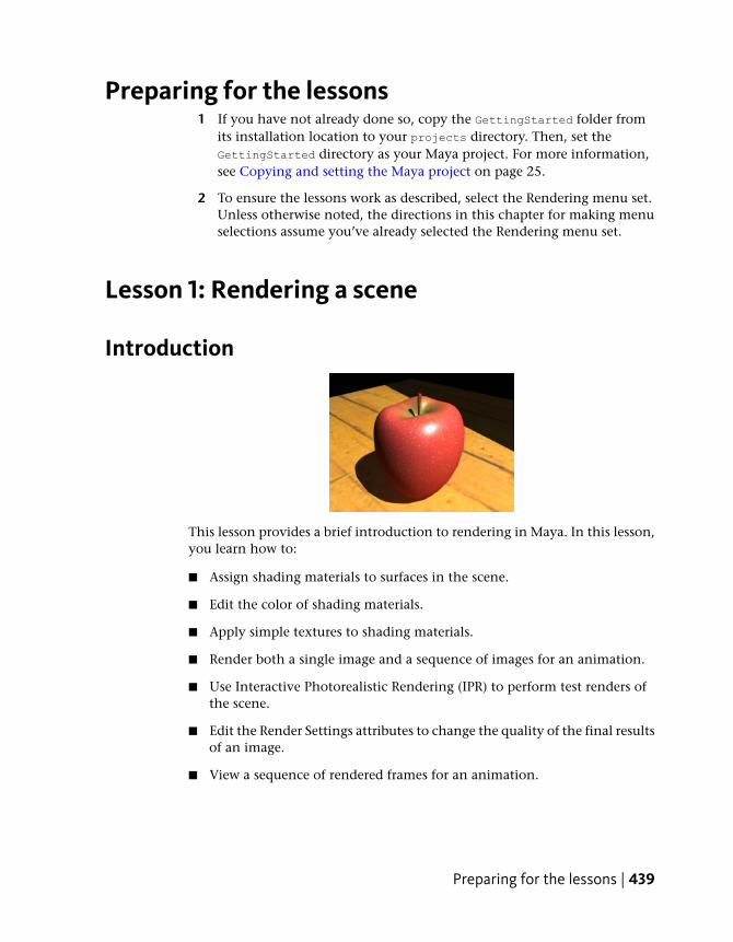
Preparing for the lessons1 If you have not already done so, copy the GettingStarted folder from
its installation location to your projects directory. Then, set theGettingStarted directory as your Maya project. For more information,see Copying and setting the Maya project on page 25.
2 To ensure the lessons work as described, select the Rendering menu set.Unless otherwise noted, the directions in this chapter for making menuselections assume you’ve already selected the Rendering menu set.
Lesson 1: Rendering a scene
Introduction
This lesson provides a brief introduction to rendering in Maya. In this lesson,you learn how to:
■ Assign shading materials to surfaces in the scene.
■ Edit the color of shading materials.
■ Apply simple textures to shading materials.
■ Render both a single image and a sequence of images for an animation.
■ Use Interactive Photorealistic Rendering (IPR) to perform test renders ofthe scene.
■ Edit the Render Settings attributes to change the quality of the final resultsof an image.
■ View a sequence of rendered frames for an animation.
Preparing for the lessons | 439

Open the scene for the lessonIn this lesson, you render a scene we’ve created for your use.
1 Make sure you’ve done the steps in Preparing for the lessons on page 439.
2 Open the scene file named apple.mb.
This file can be found in the GettingStarted directory that you set asyour Maya project:
GettingStarted\Rendering\apple.mb
The scene contains an apple sitting on a plane, with another plane as thebackground. A camera in the scene is animated to revolve around theapple at varying distances. (As an alternative to using the scene apple.mb,you can create a similar scene with your own objects.)
3 Select Window > Settings/Preferences > Preferences.
4 Click the Time Slider category and make sure the Playback Speed optionis set to Real-time (24 fps) so your animation will playback at the defaultrate of 24 frames per second.
5 Close the Preferences window.
You won’t use the animated camera until later in the lesson. In the nextsteps, you color the apple and the planes by creating shading materials.
440 | Chapter 9 Rendering

Creating shading materials for objectsA shading material is a collection of attributes that you apply to a surface tocontrol how the surface appears when it is rendered. Shading materials includesuch attributes as color, shininess, and texture. The following table outlinesthe materials you’ll be working with:
DescriptionMaterial
Creates a matte surface without specularhighlights. Lambert is the default shadingmaterial.
Lambert
Creates a shiny surface with specularhighlights, often used to simulate metallicsurfaces.
Blinn
When you open the apple.mb file, it initially displays the apple and the planesas wireframes (Shading > Wireframe). This is the default display mode forobjects in a scene view.
To create materials for the apple stem
1 In the perspective view, select Shading > Smooth Shade All (hotkey: 5).
Creating shading materials for objects | 441

The apple and the other surfaces appear with a default gray, smoothshading material, lit using default lighting. Default lighting occurs whenno other lights have been placed in the scene.
2 In the perspective view, select the apple stem by clicking its geometry.(Be sure that only the apple stem is selected.)
3 From the Rendering menu set, select Lighting/shading > Assign NewMaterial > Lambert.
The Attribute Editor appears for the Lambert material.
A Lambert material creates a matte surface without shiny highlights. Youwill learn more about materials and their attributes in a later lesson.
4 Click the gray box to the right of Color.
The Color Chooser window appears.
5 Click inside the color wheel and drag to a brown color.
The color you select in the Color Chooser is applied to the apple stem.
442 | Chapter 9 Rendering

6 Click Accept to close the window.
7 In the Attribute Editor, rename the lambert shading material toappleStem_lambert.
To create materials for the apple
1 Right-click the apple and select Assign New Material > Blinn from themarking menu.
The Attribute Editor updates to display the attributes for the Blinnmaterial.
A Blinn material gives the apple a shiny appearance.
2 Click the gray box to the right of Color.
The Color Chooser window appears.
3 Click inside the color wheel and drag to a red color.
The apple’s surface updates to the same color you select in the ColorChooser.
4 Click Accept to close the window.
5 In the Attribute Editor, rename the Blinn shading material toappleSkin_blinn.
Creating shading materials for objects | 443

To create materials for the counter and wall
1 Right-click the background plane and select Assign New Material >Lambert from the marking menu.
The Attribute Editor displays the attributes for the Lambert material.
2 Click the gray box to the right of Color.
3 In the Color Chooser window, click inside the color wheel and drag toa light blue color.
The color you select in the Color Chooser is applied to the plane.
4 Click Accept to close the window.
5 In the Attribute Editor, rename the Lambert shading material towall_lambert.
6 Right-click the surface that the apple is resting on and select Assign NewMaterial > Lambert.
The Attribute Editor displays the attributes for the Lambert material.
7 Click the gray box to the right of Color.
8 In the Color Chooser window, click inside the color wheel and drag toa beige color.
The color you select in the Color Chooser is applied to the plane.
9 Click Accept to close the window.
10 In the Attribute Editor, rename the Lambert shading material tocounter_lambert.
444 | Chapter 9 Rendering
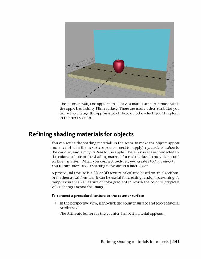
The counter, wall, and apple stem all have a matte Lambert surface, whilethe apple has a shiny Blinn surface. There are many other attributes youcan set to change the appearance of these objects, which you’ll explorein the next section.
Refining shading materials for objectsYou can refine the shading materials in the scene to make the objects appearmore realistic. In the next steps you connect (or apply) a procedural texture tothe counter, and a ramp texture to the apple. These textures are connected tothe color attribute of the shading material for each surface to provide naturalsurface variation. When you connect textures, you create shading networks.You’ll learn more about shading networks in a later lesson.
A procedural texture is a 2D or 3D texture calculated based on an algorithmor mathematical formula. It can be useful for creating random patterning. Aramp texture is a 2D texture or color gradient in which the color or grayscalevalue changes across the image.
To connect a procedural texture to the counter surface
1 In the perspective view, right-click the counter surface and select MaterialAttributes.
The Attribute Editor for the counter_lambert material appears.
Refining shading materials for objects | 445
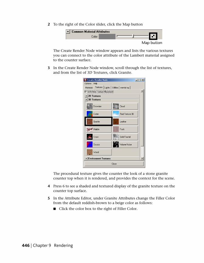
2 To the right of the Color slider, click the Map button
The Create Render Node window appears and lists the various texturesyou can connect to the color attribute of the Lambert material assignedto the counter surface.
3 In the Create Render Node window, scroll through the list of textures,and from the list of 3D Textures, click Granite.
The procedural texture gives the counter the look of a stone granitecounter top when it is rendered, and provides the context for the scene.
4 Press 6 to see a shaded and textured display of the granite texture on thecounter top surface.
5 In the Attribute Editor, under Granite Attributes change the Filler Colorfrom the default reddish-brown to a beige color as follows:
■ Click the color box to the right of Filler Color.
446 | Chapter 9 Rendering
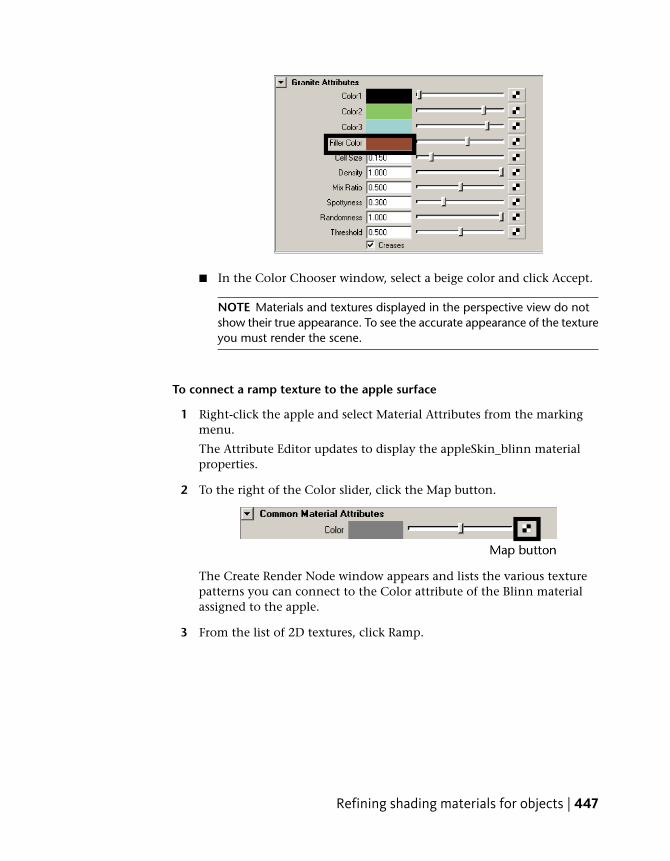
■ In the Color Chooser window, select a beige color and click Accept.
NOTE Materials and textures displayed in the perspective view do notshow their true appearance. To see the accurate appearance of the textureyou must render the scene.
To connect a ramp texture to the apple surface
1 Right-click the apple and select Material Attributes from the markingmenu.
The Attribute Editor updates to display the appleSkin_blinn materialproperties.
2 To the right of the Color slider, click the Map button.
The Create Render Node window appears and lists the various texturepatterns you can connect to the Color attribute of the Blinn materialassigned to the apple.
3 From the list of 2D textures, click Ramp.
Refining shading materials for objects | 447
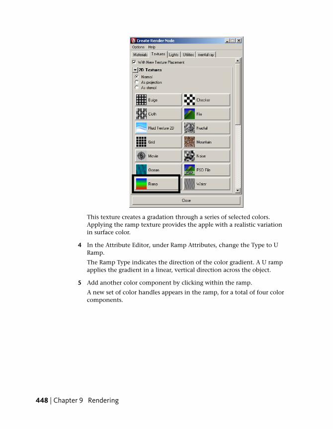
This texture creates a gradation through a series of selected colors.Applying the ramp texture provides the apple with a realistic variationin surface color.
4 In the Attribute Editor, under Ramp Attributes, change the Type to URamp.
The Ramp Type indicates the direction of the color gradient. A U rampapplies the gradient in a linear, vertical direction across the object.
5 Add another color component by clicking within the ramp.
A new set of color handles appears in the ramp, for a total of four colorcomponents.
448 | Chapter 9 Rendering

6 To change the ramp colors, click the top circular color handle (to indicatewhich color you want to modify), then click the color box to the rightof Selected Color to display the Color Chooser window.
7 Click inside the color wheel and drag to a very dark brown for the firstramp color. Click Accept to close the window.
8 Repeat steps 6 and 7 for the other three ramp colors. For the two middleramp colors, select a dark red. For the last ramp color, select a deep olivegreen.
9 Click Accept to close the window.
10 Use the circular color handles to reposition each component as shownbelow:
Refining shading materials for objects | 449

The position of these handles and the corresponding colors affect thelocation and breadth of the color within the gradient on the apple’ssurface.
11 Save your work.
In the next section you render your scene to view the textures andmaterials you’ve assigned to the objects.
Maya renderersSo far, you’ve seen the results of shading the apple and other surfaces in thescene view. In this view, Maya uses your computer’s graphics hardware todisplay the shading and textures quickly but with low quality.
To view the shading results of the colors and textures in a more realisticfashion, you must use a renderer. In this lesson you use a process called softwarerendering.
Software rendering can take seconds or minutes to render a single frame ofanimation from your scene, depending on the complexity of surface geometry,shaders, lighting and other visual elements present in the scene.
The following table outlines the different types of renderers in Maya and whateach is used for:
UseRenderer
A general purpose renderer with broadcapabilities. You can produce high-quality
Maya’s Software renderer
images with complex shading networks,including procedural textures and ramps.Software rendering is computed throughyour machine’s processor.
450 | Chapter 9 Rendering
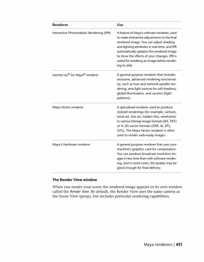
UseRenderer
A feature of Maya’s software renderer, usedto make interactive adjustments to the final
Interactive Photorealistic Rendering (IPR)
rendered image. You can adjust shadingand lighting attributes in real-time, and IPRautomatically updates the rendered imageto show the effects of your changes. IPR isuseful for tweaking an image before render-ing to disk.
A general purpose renderer that includesexclusive, advanced rendering functional-
mental ray® for Maya® renderer
ity, such as host and network parallel ren-dering, area light sources for soft shadows,global illumination, and caustics (lightpatterns).
A specialized renderer used to producestylized renderings (for example, cartoon,
Maya Vector renderer
tonal art, line art, hidden line, wireframe)in various bitmap image formats (IFF, TIFF)or in 2D vector formats (SWF, AI, EPS,SVG). The Maya Vector renderer is oftenused to render web-ready images.
A general purpose renderer that uses yourmachine’s graphics card for computation.
Maya’s Hardware renderer
You can produce broadcast resolution im-ages in less time than with software render-ing, and in some cases, the quality may begood enough for final delivery.
The Render View window
When you render your scene the rendered image appears in its own windowcalled the Render View. By default, the Render View uses the same camera asthe Scene View (persp), but includes particular rendering capabilities.
Maya renderers | 451
The following table shows the differences between the Render View and theScene View:
Render ViewScene View
2D rendered image3D object sceneDisplay
shaded surfaces onlymodeled surfaces, the grid,vertices, curves, and objectmanipulators
Surfaces
black background by de-fault because only objects
default gray backgroundBackground
with materials that are litcan be seen
high-quality, colors andtextures appear in their fi-nal rendered form
low-quality, colors and tex-tures do not appear in theirfinal display form
Quality
Rendering a single frame using IPRIn this section, you work with IPR (Interactive Photorealistic Rendering), atype of software rendering.
The advantage of rendering with IPR is that, after you render an image, youcan adjust the shading and lighting attributes of the scene and then quicklyupdate part or all of the rendered image to review the effect of your changes.IPR is useful for iterations when you need to fine-tune specific attributes.Updates to the image are not always instantaneous, but they are full quality.
To render the scene using IPR
1 In the perspective view, select View > Camera Attribute Editor to displaythe attributes for the camera.
You need to specify the exact region of the perspective view you want torender.
2 In the Attribute Editor, open the Display Options section and turn onDisplay Resolution.
A dark green rectangular border shows the region to be rendered. Thisregion defines the area of the final image, and allows you to decide what
452 | Chapter 9 Rendering
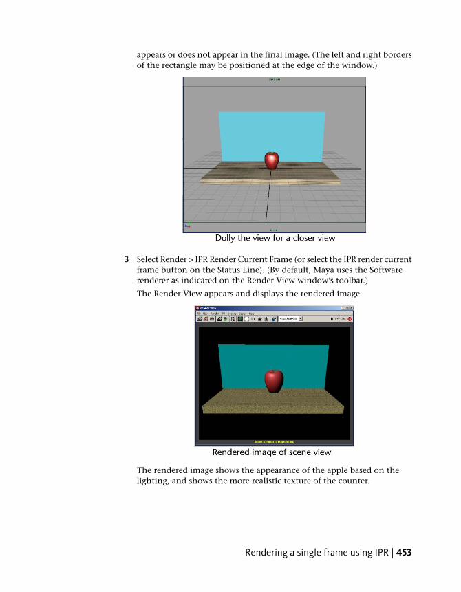
appears or does not appear in the final image. (The left and right bordersof the rectangle may be positioned at the edge of the window.)
3 Select Render > IPR Render Current Frame (or select the IPR render currentframe button on the Status Line). (By default, Maya uses the Softwarerenderer as indicated on the Render View window’s toolbar.)
The Render View appears and displays the rendered image.
The rendered image shows the appearance of the apple based on thelighting, and shows the more realistic texture of the counter.
Rendering a single frame using IPR | 453
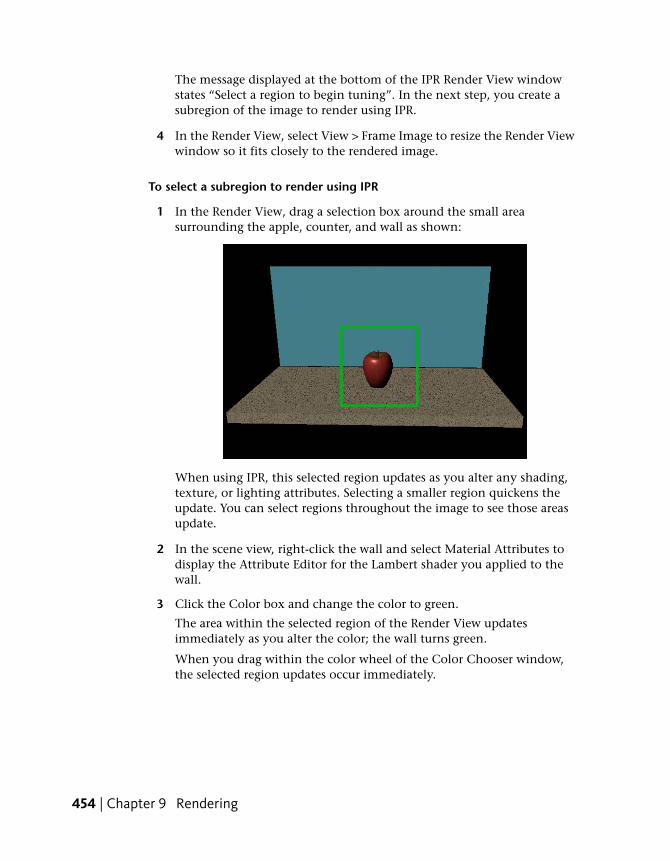
The message displayed at the bottom of the IPR Render View windowstates “Select a region to begin tuning”. In the next step, you create asubregion of the image to render using IPR.
4 In the Render View, select View > Frame Image to resize the Render Viewwindow so it fits closely to the rendered image.
To select a subregion to render using IPR
1 In the Render View, drag a selection box around the small areasurrounding the apple, counter, and wall as shown:
When using IPR, this selected region updates as you alter any shading,texture, or lighting attributes. Selecting a smaller region quickens theupdate. You can select regions throughout the image to see those areasupdate.
2 In the scene view, right-click the wall and select Material Attributes todisplay the Attribute Editor for the Lambert shader you applied to thewall.
3 Click the Color box and change the color to green.
The area within the selected region of the Render View updatesimmediately as you alter the color; the wall turns green.
When you drag within the color wheel of the Color Chooser window,the selected region updates occur immediately.
454 | Chapter 9 Rendering

NOTE If the region does not update, in the Render Settings window, turnthe Raytracing option off.
(You won’t alter any other attributes in this lesson. The purpose of thelesson is to learn the process of rendering, not to perfect the results atthis point.)
4 From the Render View menu, select IPR > Redo Previous IPR Render.
The rendered image updates to the full resolution.
By default, the resolution of the IPR window is 320 by 240 pixels. Theadvantage of this relatively small resolution is that it renders quickly. However,if you want a larger image, you can increase the image resolution.
To increase the size of the rendered image
1 In the Render View menu, select Options > Render Settings (or click theRender Settings button in the Render View window).
The Render Settings window appears.
Rendering a single frame using IPR | 455
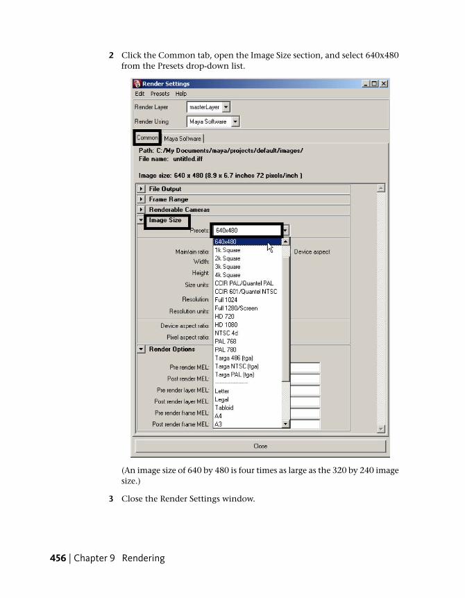
2 Click the Common tab, open the Image Size section, and select 640x480from the Presets drop-down list.
(An image size of 640 by 480 is four times as large as the 320 by 240 imagesize.)
3 Close the Render Settings window.
456 | Chapter 9 Rendering
4 Close the Render View window.
5 Select Render > IPR Render Current Frame (or select the IPR render currentframe button on the Status Line).
The Render View window opens and renders an image with an imagesize of 640 by 480 pixels.
NOTE If you are using Maya on Windows or Linux, rendering the scenedisplays another window called the Output window, typically behind otherwindows on your desktop. The Output window lists statistics about the imagejust rendered. For now, you can ignore and close the Output window. Itcontains information that you will appreciate more as you gain experienceusing Maya.
So far, you’ve used IPR to see changes you made to a shader. If you add lightsto the scene rather than using default lighting, you can also use IPR to helpadjust the lighting.
Rendering using the Maya software rendererYou are nearly ready to render the entire animation to disk. You must firstswitch camera views so you can render the scene from the point of view ofthe camera that was animated for this lesson. When animating a camera it’sa good practice to create a second camera to animate, rather than animatingthe default persp camera. In that way you can return to the default perspectiveview should it become necessary.
Rendering the entire animation can take a lot of time, so it is useful to firstuse Maya’s software renderer to test render a few frames to your monitor andexamine the results.
Once you are satisfied with the quality of a few rendered frames, you canrender the entire animation to disk.
To switch camera views and playback the animation
1 In the perspective view, select Panels > Perspective > apple_camera.
The view updates to display the scene as seen through the lens of theapple_camera.
2 Click the Play button in the Timeslider playback controls.
During playback, the animated camera tracks and tumbles about theapple.
Rendering using the Maya software renderer | 457
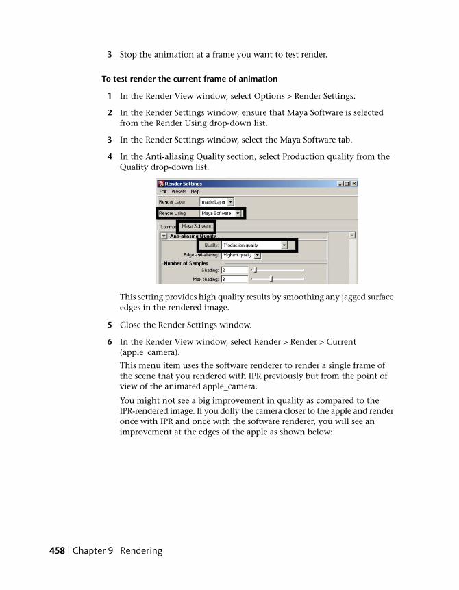
3 Stop the animation at a frame you want to test render.
To test render the current frame of animation
1 In the Render View window, select Options > Render Settings.
2 In the Render Settings window, ensure that Maya Software is selectedfrom the Render Using drop-down list.
3 In the Render Settings window, select the Maya Software tab.
4 In the Anti-aliasing Quality section, select Production quality from theQuality drop-down list.
This setting provides high quality results by smoothing any jagged surfaceedges in the rendered image.
5 Close the Render Settings window.
6 In the Render View window, select Render > Render > Current(apple_camera).
This menu item uses the software renderer to render a single frame ofthe scene that you rendered with IPR previously but from the point ofview of the animated apple_camera.
You might not see a big improvement in quality as compared to theIPR-rendered image. If you dolly the camera closer to the apple and renderonce with IPR and once with the software renderer, you will see animprovement at the edges of the apple as shown below:
458 | Chapter 9 Rendering

7 Go to frame 120 of the animation, where the apple is viewed in a differentposition.
8 In the Render View, select Render > Render > Current (apple_camera).
Ensure that the rendered image looks good at this frame also.
Now that you’ve checked a pair of rendered frames that represent the entireanimation, you are ready to render the entire animation sequence. In yourown projects, you might want to test render several frames, particularly wherenew shading and lighting elements occur in the animation.
Batch rendering a sequence of animation framesAfter you model, animate, and color your scene, you set several Render Settingsoptions and then use the software renderer to batch render part or all of theanimation’s range of frames to files on disk. Each file represents a single frame(image) of the animation.
To set the Render Settings for batch rendering
1 In the Render View window, select Options > Render Settings to displaythe Render Settings window.
2 In the Render Settings window, select the Common tab, and then openthe File Output section.
3 In the File Output section, set the following options:
■ File Name Prefix: Type the name Apple. This name will be the baseof the filenames created by batch rendering.
■ Image Format: Select Maya IFF (.iff), Maya’s standard image file format.You can use the .iff format for any further work you need to do,
Batch rendering a sequence of animation frames | 459
including previewing and compositing the animation. If you requirea different format, you can specify it instead of .iff in the RenderSettings.
■ Frame/Animation Ext: Select name.#.ext. This specifies that thefilenames will have the format prefix.frameNumber.fileFormat. Forexample, batch rendering the entire 200-frame animation will createApple.0001.iff, Apple.0002.iff, and so on through Apple.00200.iff.
■ Frame padding: Enter 4. This causes the frameNumber part of thefilenames to be four digits prefixed with 0s. For example, the filenameswill be Apple.0001.iff through Apple.0050.iff.
■ Start frame: Enter 1, the first frame of the animation sequence to bebatch rendered.
■ End frame: Enter 60, the last frame to be batch rendered. (Renderingall 200 frames may be time-consuming.)
■ Renderable Camera: Select apple_camera from the drop-down list toindicate which camera view to render.
The four-digit padded filename is compatible with many image playbackprograms, for example, Maya’s FCheck utility. Image playback programslet you view rendered animation sequences on your monitor at real-timespeed.
For the remaining options in the Render Settings window, you’ll use thedefault settings. Maya will render using the image size (640x480), andanti-aliasing quality (Production Quality) that you specified earlier in thelesson.
After you set the Render Settings, the top portion of the Common tabshows the correct path and filenames for the files to be created duringbatch rendering. Check that this information is correct.
460 | Chapter 9 Rendering

4 Close the Render Settings window.
To batch render animation frames
1 Save the scene.
It’s a good practice to save the scene before batch rendering. This is usefulif, after batch rendering, you need to change any display settings andrender again. By saving the scene prior to batch rendering, you canexamine the scene to learn which option settings were in effect at thetime you batch rendered.
2 From the Rendering menu set, select Render > Batch Render > .
The Batch Render Frame window appears.
3 Turn on Use all available processors, then click Batch Render and closeto start batch rendering.
(The Use all available processors option allows Maya to use all theprocessors available on the local machine to complete the render.)
Batch rendering a sequence of animation frames | 461
NOTE For users of Maya Personal Learning Edition, the Use all AvailableProcessors option is disabled. Use the default settings.
Batch rendering 50 frames of a simple scene takes a few minutes. Acomplex scene may take hours per frame, depending on the speed ofyour computer.
To check the status of the batch render
1 While Maya is rendering, select Window > General Editors > Script Editor.Expand the size of the Script Editor window. The window shows acompletion log for the frames being rendered.
Maya puts the resulting files in a default images directory. The files havethe following names:
Apple.0001.iff
Apple.0002.iff
Apple.0003.iff
...
...
Apple.0050.iff
The images directory is located in the same path as the scenes directory.You can have Maya save to a different path by changing the projectsetting. See the Maya Help for further information on projects.
2 Close the Script Editor when the following message appears:
// Result: Rendering Completed. See mayaRenderLog.txt for inform
ation. //
The mayaRenderLog.txt file contains rendering statistics for advancedusers.
Viewing a sequence of rendered framesYou can use Maya’s FCheck image viewing utility to view the batch-renderedimages at a speed that approximates video or film.
To use FCheck to view a sequence of rendered frames
1 Select File > View Sequence.
The File Browser window appears.
462 | Chapter 9 Rendering

2 Using the File Browser, navigate to the images directory for your currentproject (or wherever you saved the rendered sequence of images for theApple).
3 Click the image file Apple.0001.iff to select the first image in thesequence and then click Open.
The FCheck image viewing utility appears and the rendered sequence of60 frames plays back as an animated loop.
4 Close the window after viewing the animation.
NOTE The FCheck rendering utility has playback, display, and other optionsyou can select from your keyboard. Details are available from the FCheckHelp menu.
Beyond the lessonIn this lesson, you were introduced to some of the basic concepts for renderingan image. In this lesson you learned that:
■ Surfaces are assigned shading materials to provide basic attributes such ascolor, shininess, reflectivity, and so on. Each shading material has uniquecharacteristics that can be modified to suit your requirements.
■ You can additionally assign a texture map to some of the shading materialattributes so that your objects appear more realistic.
■ Maya provides several methods for rendering an image. You can renderusing the Maya Software renderer, the Maya Hardware renderer, the MayaVector renderer or the mental ray® for Maya® renderer. Each type ofrenderer has specific advantages and uses.
■ You can choose the size and quality for a rendered image prior to renderingbased on your specific needs and requirements.
■ You can render a single image or a sequence of images from an animation.
■ You can view one image, or a sequence of rendered frames using the FCheckutility.
As you render scenes, consider the following issues:
Beyond the lesson | 463

Using IPR
There are a few limitations to using IPR for fast visual feedback as you adjustshading and lighting. Besides being unable to provide production-qualityanti-aliasing, IPR cannot display several other advanced display characteristics,for example, true surface reflections (raytracing) and 3D motion blur. If anadvanced display characteristic seems to be missing from an IPR-renderedframe, try rendering the frame with the software renderer.
If you change the camera view, turn Depth Map Shadows on or off, orreposition shadows, IPR does not update the rendered image automatically.You must refresh the image. From the Render View window, select IPR >Refresh IPR Image.
Batch rendering
In this lesson, you used the Maya software renderer to check the image qualityof two frames before you started to batch render. When you create scenes withsophisticated animation, it’s useful to batch render with low-quality resolutionto check the animation accuracy before batch rendering withproduction-quality resolution. For instance, you might preview your animationwith the frames resulting from batch rendering at a small image size (320 by240) with Preview Quality anti-aliasing.
You don’t need to use the batch renderer to render single frames from yourscene to disk. From the Render View window, select File > Save Image.
Hardware rendering
Hardware rendering leverages the power provided by hardware graphics cardsto render your images. The benefits of hardware rendering include the abilityto batch render frames more quickly than with software rendering, andrendering specific particle effects not possible through software rendering. Insome cases, the image quality may be good enough for final use. You accessthe hardware renderer by selecting Render > Render Using > Maya Hardware.
Hardware rendering has its own limitations when compared to softwarerendering. For more information on hardware rendering, see the Maya Help.
Rendering in layers
It’s often useful to render objects in your scene in different layers and combinethem using compositing software. In some cases, you must render some opticaleffects and then composite them afterwards. Rendering in layers can end upbeing faster than rendering an entire scene, and it lets you replace individualobjects quickly if the need arises. To set up layers, use the Layer Editor, which
464 | Chapter 9 Rendering
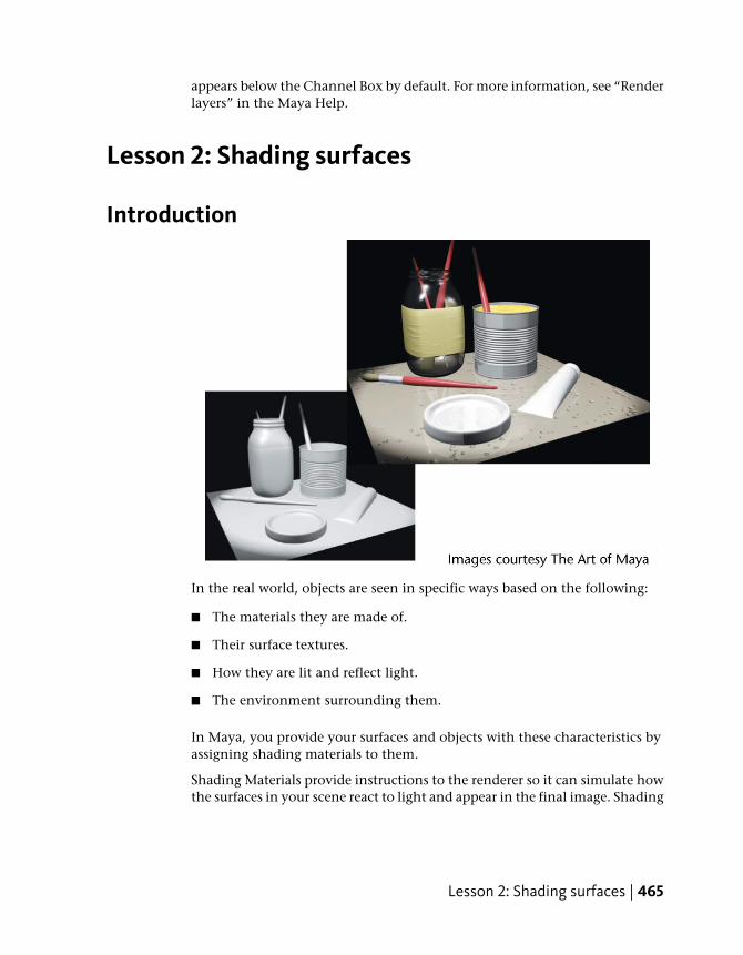
appears below the Channel Box by default. For more information, see “Renderlayers” in the Maya Help.
Lesson 2: Shading surfaces
Introduction
In the real world, objects are seen in specific ways based on the following:
■ The materials they are made of.
■ Their surface textures.
■ How they are lit and reflect light.
■ The environment surrounding them.
In Maya, you provide your surfaces and objects with these characteristics byassigning shading materials to them.
Shading Materials provide instructions to the renderer so it can simulate howthe surfaces in your scene react to light and appear in the final image. Shading
Lesson 2: Shading surfaces | 465

involves such attributes as color, transparency, shininess, and many othersto create a realistic look.
Editing the material attributes associated with shading materials affects howthey appear in the rendered image. In this way, Maya provides the option ofallowing you to create images as they would appear in the real world or inyour imagination.
In this lesson, you learn to use basic shading features to render a sphere so itappears like an orange in the final image.
In this lesson you learn how to:
■ Assign a shading material with specific color and surface attributes.
■ Differentiate between shading material types (Lambert, Blinn, Phong, andso on) to achieve a specific material appearance.
■ Assign a label texture map to a surface.
■ Use the Hypershade editor to view and work with shading materials.
■ Create a bump texture map to simulate the orange’s pebbled skin.
■ Control the placement of a 3D texture using a 3D manipulator.
Open the scene for the lessonIn this lesson, you work with a scene we created for your use.
1 Make sure you’ve done the steps in Preparing for the lessons on page 439.
2 Open the scene file named ShadeOrange.mb.
This file can be found in the GettingStarted directory that you set asyour Maya project:
GettingStarted\Rendering\ShadeOrange.mb
This scene contains a sphere modeled to resemble an orange.
466 | Chapter 9 Rendering

The scene’s perspective view also has two settings turned on—Shading >Smooth Shade All and Shading > Hardware Texturing (Hotkey: 6)—whichlet you see the shading changes you are about to make.
Assigning a shading materialIn the next steps, you create a material and assign it to the surface. A materialis a collection of attributes that define color, shininess, and other surfacecharacteristics.
To assign a material to an object
1 Before you create a new material, right-click the sphere and select MaterialAttributes.
The default material attributes appear in the Attribute Editor.
The default material assigned to the sphere (and all other surfaces) is atype of material called Lambert. The material displays the surface withgray shading. You should not edit the default shading material.
2 Right-click the sphere and select Assign New Material > Blinn to create anew material for the sphere.
The new material’s attributes appear in the Attribute Editor.
A Blinn material gives a surface a shinier look than a Lambert material.Blinn is a good choice for creating a variety of surface appearances.Knowing which material type to use for a particular surface comes withpractice. Fortunately, you can change the material type later on, so youdo not need to make a decision now. You will learn more about materialtypes later in the lesson.
3 In the Attribute Editor, click the gray box to the right of Color to openthe Color Chooser.
Assigning a shading material | 467
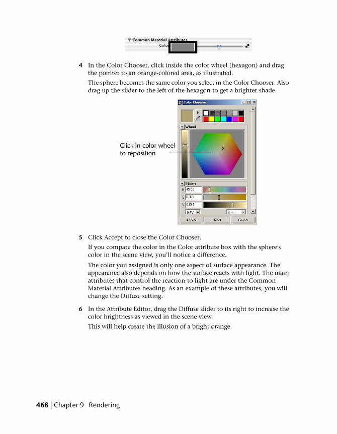
4 In the Color Chooser, click inside the color wheel (hexagon) and dragthe pointer to an orange-colored area, as illustrated.
The sphere becomes the same color you select in the Color Chooser. Alsodrag up the slider to the left of the hexagon to get a brighter shade.
5 Click Accept to close the Color Chooser.
If you compare the color in the Color attribute box with the sphere’scolor in the scene view, you’ll notice a difference.
The color you assigned is only one aspect of surface appearance. Theappearance also depends on how the surface reacts with light. The mainattributes that control the reaction to light are under the CommonMaterial Attributes heading. As an example of these attributes, you willchange the Diffuse setting.
6 In the Attribute Editor, drag the Diffuse slider to its right to increase thecolor brightness as viewed in the scene view.
This will help create the illusion of a bright orange.
468 | Chapter 9 Rendering
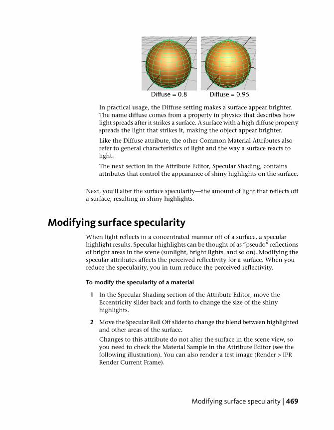
In practical usage, the Diffuse setting makes a surface appear brighter.The name diffuse comes from a property in physics that describes howlight spreads after it strikes a surface. A surface with a high diffuse propertyspreads the light that strikes it, making the object appear brighter.
Like the Diffuse attribute, the other Common Material Attributes alsorefer to general characteristics of light and the way a surface reacts tolight.
The next section in the Attribute Editor, Specular Shading, containsattributes that control the appearance of shiny highlights on the surface.
Next, you’ll alter the surface specularity—the amount of light that reflects offa surface, resulting in shiny highlights.
Modifying surface specularityWhen light reflects in a concentrated manner off of a surface, a specularhighlight results. Specular highlights can be thought of as “pseudo” reflectionsof bright areas in the scene (sunlight, bright lights, and so on). Modifying thespecular attributes affects the perceived reflectivity for a surface. When youreduce the specularity, you in turn reduce the perceived reflectivity.
To modify the specularity of a material
1 In the Specular Shading section of the Attribute Editor, move theEccentricity slider back and forth to change the size of the shinyhighlights.
2 Move the Specular Roll Off slider to change the blend between highlightedand other areas of the surface.
Changes to this attribute do not alter the surface in the scene view, soyou need to check the Material Sample in the Attribute Editor (see thefollowing illustration). You can also render a test image (Render > IPRRender Current Frame).
Modifying surface specularity | 469
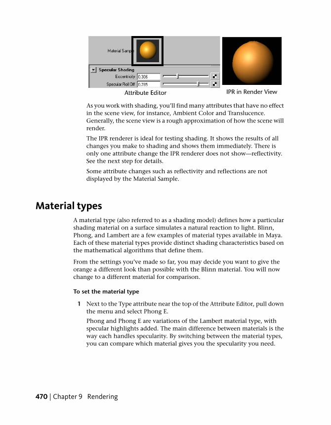
As you work with shading, you’ll find many attributes that have no effectin the scene view, for instance, Ambient Color and Translucence.Generally, the scene view is a rough approximation of how the scene willrender.
The IPR renderer is ideal for testing shading. It shows the results of allchanges you make to shading and shows them immediately. There isonly one attribute change the IPR renderer does not show—reflectivity.See the next step for details.
Some attribute changes such as reflectivity and reflections are notdisplayed by the Material Sample.
Material typesA material type (also referred to as a shading model) defines how a particularshading material on a surface simulates a natural reaction to light. Blinn,Phong, and Lambert are a few examples of material types available in Maya.Each of these material types provide distinct shading characteristics based onthe mathematical algorithms that define them.
From the settings you’ve made so far, you may decide you want to give theorange a different look than possible with the Blinn material. You will nowchange to a different material for comparison.
To set the material type
1 Next to the Type attribute near the top of the Attribute Editor, pull downthe menu and select Phong E.
Phong and Phong E are variations of the Lambert material type, withspecular highlights added. The main difference between materials is theway each handles specularity. By switching between the material types,you can compare which material gives you the specularity you need.
470 | Chapter 9 Rendering
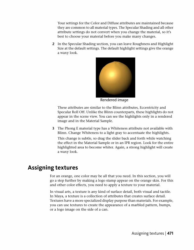
Your settings for the Color and Diffuse attributes are maintained becausethey are common to all material types. The Specular Shading and all otherattribute settings do not convert when you change the material, so it’sbest to choose your material before you make many changes.
2 In the Specular Shading section, you can leave Roughness and HighlightSize at the default settings. The default highlight settings give the orangea waxy look.
These attributes are similar to the Blinn attributes, Eccentricity andSpecular Roll Off. Unlike the Blinn counterparts, these highlights do notappear in the scene view. You can see the highlights only in a renderedimage and in the Material Sample.
3 The Phong E material type has a Whiteness attribute not available withBlinn. Change Whiteness to a light gray to accentuate the highlights.
This change is subtle, so drag the slider back and forth while watchingthe effect in the Material Sample or in an IPR region. Look for the entirehighlighted area to become whiter. Again, a strong highlight will createa waxy look.
Assigning texturesFor an orange, one color may be all that you need. In this section, you willgo a step further by making a logo stamp appear on the orange skin. For thisand other color effects, you need to apply a texture to your material.
In visual arts, a texture is any kind of surface detail, both visual and tactile.In Maya, a texture is a collection of attributes that creates surface detail.Textures have a more specialized display purpose than materials. For example,you can use textures to create the appearance of a marbled pattern, bumps,or a logo image on the side of a can.
Assigning textures | 471

In the Maya Help, a texture is also referred to as a texture node. A node is acollection of attributes (or actions) with a common purpose. A shader issometimes called a shader node or material node.
To display a texture on a surface, you apply a texture node to an attribute ofthe surface material. In the next steps, you apply a texture to the Color attributeof the Phong E material.
To apply a texture to a material
1 Click the Map button next to the Color slider. This is a quick way ofapplying a texture to an attribute. This is also called mapping a texture.
The Create Render Node window displays a list of the textures you canapply. The texture names and their icons help you to decide which textureis appropriate for the effect you want.
To create the logo stamp effect, you will use the File texture. A File textureuses an image file that you or someone else created separately, such as adrawing from a paint program. For this lesson, you’ll use an image wecreated for you.
2 Before you create the texture, make sure Normal is selected in the optionsabove the texture swatches.
472 | Chapter 9 Rendering

The Normal option means Maya will stretch the texture evenly aroundthe surface. The other settings—Projection and Stencil—are other waysyou can apply a texture. You will learn about these settings at the end ofthe lesson.
3 In the 2D Textures list, click the File button once.
At this point the system may prompt you with the warning that “TheIPR file does not have enough information to support your most recentchange”. Select “Close the IPR file and stop tuning”. The file1 nodeappears in the Attribute Editor.
The file texture also causes the sphere to turn white in the scene viewand black in a rendered view. This is a temporary color until you specifythe actual file name of the file texture.
4 Click the folder icon to the right of the Image Name attribute. A browserwindow opens with the path set to a default directory called sourceimages.
Maya looks for source images in a default sourceimages directory.However, Maya can use file texture images anywhere on your workstationor local network. For example, you could have them on a central diskdrive that is shared among your coworkers.
5 Navigate to the GettingStarted\Rendering\sourceimages directory andopen Render_Mayakist.iff.
6 In the Render View window select IPR > Redo Previous IPR Render.
The file texture with a Mayakist logo now appears on the sphere. Thelogo is somewhat jagged, which will simulate the look of an ink stampon rough orange skin.
7 In the Attribute Editor, click the place2dTexture1 tab.
The place2dTexture1 tab is a node with attributes that control the texture’sposition on the surface.
Assigning textures | 473
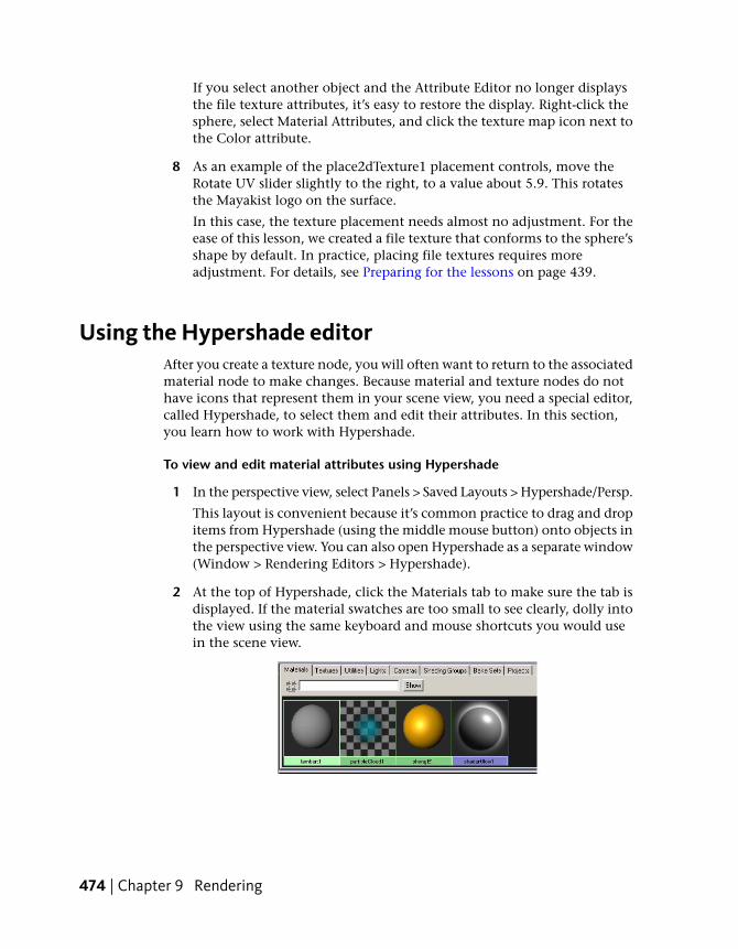
If you select another object and the Attribute Editor no longer displaysthe file texture attributes, it’s easy to restore the display. Right-click thesphere, select Material Attributes, and click the texture map icon next tothe Color attribute.
8 As an example of the place2dTexture1 placement controls, move theRotate UV slider slightly to the right, to a value about 5.9. This rotatesthe Mayakist logo on the surface.
In this case, the texture placement needs almost no adjustment. For theease of this lesson, we created a file texture that conforms to the sphere’sshape by default. In practice, placing file textures requires moreadjustment. For details, see Preparing for the lessons on page 439.
Using the Hypershade editorAfter you create a texture node, you will often want to return to the associatedmaterial node to make changes. Because material and texture nodes do nothave icons that represent them in your scene view, you need a special editor,called Hypershade, to select them and edit their attributes. In this section,you learn how to work with Hypershade.
To view and edit material attributes using Hypershade
1 In the perspective view, select Panels > Saved Layouts > Hypershade/Persp.
This layout is convenient because it’s common practice to drag and dropitems from Hypershade (using the middle mouse button) onto objects inthe perspective view. You can also open Hypershade as a separate window(Window > Rendering Editors > Hypershade).
2 At the top of Hypershade, click the Materials tab to make sure the tab isdisplayed. If the material swatches are too small to see clearly, dolly intothe view using the same keyboard and mouse shortcuts you would usein the scene view.
474 | Chapter 9 Rendering

This tab shows all the materials currently in your scene. It is especiallyuseful when you have a complex scene and you need to locate a materialto edit it. The materials you will recognize are the default Lambert materialand the Phong E material. You can ignore the others. They exist in allscenes, by default, for use with other Maya features.
In addition to the Materials tab, Hypershade includes other tabs to helpyou keep track of textures, lights, and other nodes related to rendering.
3 With the middle mouse button, drag the lambert1 swatch into the sceneview and over the sphere. When you release the mouse, the Lambertmaterial appears on the sphere instead of the Phong E material youpreviously created.
4 Drag the phongE1 swatch onto the sphere to reapply that material.
Hypershade is designed for quick, drag-and-drop operations such as this.
5 Select the sphere.
6 From the menus in Hypershade, select Graph > Graph Materials onSelected Objects.
A graph appears in the Work Area tab in the bottom section.
Using the Hypershade editor | 475

This graph shows all material and texture nodes applied to this object.While the Materials tab shows a catalog of the materials in the scene, theWork Area tab shows whatever material, texture, or other node you arecurrently working on. The Graph menu has several menu items thatchange the contents of the Work Area display.
The Shader Library tab shown in the above illustration might not be apart of your Maya installation. It is an optional feature, discussed at theend of this lesson.
The Work Area shows connection lines between the nodes. The lineshave arrows that all point in one direction. For a closer look at thesearrows, dolly into the view using the same keyboard and mouse shortcutsyou would use in the scene view.
The arrows depict Maya’s internal information input and output, calleda stream. The next step shows the importance of this connection stream.
7 Click the line between the file1 and phongE1 nodes (it turns yellow) andpress the Delete key.
The sphere reverts to the default gray color because you have broken theconnection between these nodes and the texture is no longer assignedto it. This is a simple illustration of how the connection stream works.The file1 texture node is upstream from the connection you deleted, soit no longer inputs data into the material; Maya ignores it.
In practical terms, this is an example of how you can disconnect a texturefrom a material without actually deleting the texture. For example, youmay want to remove the file texture from this material and connect it toanother material instead. In a later step, you will learn about usingHypershade to make connections between textures and materials.
476 | Chapter 9 Rendering
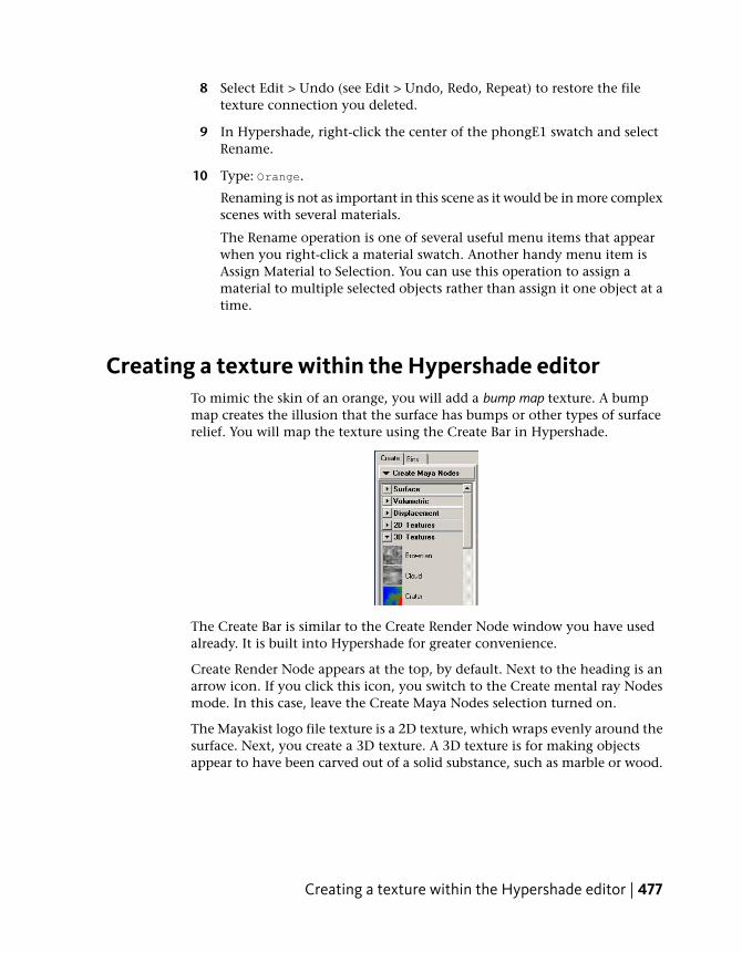
8 Select Edit > Undo (see Edit > Undo, Redo, Repeat) to restore the filetexture connection you deleted.
9 In Hypershade, right-click the center of the phongE1 swatch and selectRename.
10 Type: Orange.
Renaming is not as important in this scene as it would be in more complexscenes with several materials.
The Rename operation is one of several useful menu items that appearwhen you right-click a material swatch. Another handy menu item isAssign Material to Selection. You can use this operation to assign amaterial to multiple selected objects rather than assign it one object at atime.
Creating a texture within the Hypershade editorTo mimic the skin of an orange, you will add a bump map texture. A bumpmap creates the illusion that the surface has bumps or other types of surfacerelief. You will map the texture using the Create Bar in Hypershade.
The Create Bar is similar to the Create Render Node window you have usedalready. It is built into Hypershade for greater convenience.
Create Render Node appears at the top, by default. Next to the heading is anarrow icon. If you click this icon, you switch to the Create mental ray Nodesmode. In this case, leave the Create Maya Nodes selection turned on.
The Mayakist logo file texture is a 2D texture, which wraps evenly around thesurface. Next, you create a 3D texture. A 3D texture is for making objectsappear to have been carved out of a solid substance, such as marble or wood.
Creating a texture within the Hypershade editor | 477

To create a bump texture within the Hypershade Editor
1 In the Create bar, scroll down to the 3D Textures heading.
For this bump effect, you use a Brownian 3D texture. Experience hasshown that a Brownian texture is the best texture for approximating thebumps on an orange skin. Becoming skillful with textures is a matter ofobservation, experimentation, and experience.
2 With the middle mouse button, drag the Brownian texture (under 3DTextures) onto the Orange material swatch in the Work Area tab andrelease the mouse button.
3 From the menu that appears, choose bump map.
Maya connects or applies Brownian to the Orange material’s bump mapattribute.
The pop-up menu shows a list of common material attributes. Althoughyou can map textures to any material attribute, these are the mostcommonly mapped attributes.
By default, you can assign only one texture per attribute. Attributes thatalready have an assigned texture appear in italics. (For a discussion aboutassigning multiple textures to an attribute, see Layered textures on page483.)
This drag-and-drop method of applying a texture is essentially the sameas clicking the map icon next to a material’s attribute slider. UsingHypershade offers a faster, more graphical alternative to using theAttribute Editor.
4 Select Graph > Input and Output Connections to view the nodeconnections for the new texture you created.
478 | Chapter 9 Rendering

Also notice that bumps from the bump map appear in the Orangematerial’s swatch. The Orange material swatch is the same as the MaterialSample that appears in the Attribute Editor for the material node. (Thebumps also appear in a rendered image, but not in the scene view.)
5 Double-click the bump3d1 swatch (the checkered cube) to display itsattributes in the Attribute Editor.
This node is the link between the texture and the material. It convertsvisual information, such as the mottled Brownian pattern, into theappearance of surface relief.
The most important attribute in the bump3d1 node is Bump Depth,which controls the intensity of the bumps.
6 Change Bump Depth to 0.15. In the Orange swatch or a rendered image,you’ll see that this diminishes the bumps as compared to the defaultvalue 1.0.
NOTE If you select Render > IPR Render Current Frame while Hypershade isselected, a message appears: Please select the view you want to render. Eitherselect the perspective view before choosing IPR Render Current Frame, or,in the Render View window, select IPR > Redo Previous IPR Renderer.
7 In the Hypershade panel, click the brownian1 texture swatch to revealits attributes. Set the following:
■ Increment: 0.3
■ Octaves: 4.0
These values produce a rendered image closer to real orange skin.
Creating a texture within the Hypershade editor | 479

Our recommendation for these values is based on experimentation. ForBrownian and some other textures, it’s usually faster to get desirableresults by experimenting with the settings rather than trying tounderstand the definition of each attribute.
Modifying a bump textureThe bump texture is too crater-like to be a convincing orange. The bumps aretoo numerous and too deep. A quick way to fix this problem is to scale up theentire texture.
To interactively position a 3D texture
1 Double click the place3dTexture1 swatch, to the left of the Browniancolor swatch.
This node controls the 3D texture’s position, scale, and rotation. Thevisual display of this node is a large cube that surrounds the sphere inthe scene view. This is the texture placement cube.
2 Click the Interactive Placement button in the Attribute Editor. Amanipulator appears for the texture placement cube.
480 | Chapter 9 Rendering

3 In the scene view, click on the center scale box to activate the centerscale option. Scale the whole texture placement cube to about twice theoriginal size (until the Scale attribute values are about 2).
Now when you render, the bumps on the surface appear wider andsmoother, like the bumps on an orange skin. For example, the bumps inthe area surrounding the highlight do not appear to be as deep as theywere before you scaled the texture.
Scaling a texture placement cube is a common way to tune the texture’sdisplay. Scaling does not actually change the pattern, but enlarges orshrinks it relative to the surface.
4 Now that you’ve changed the surface texture through scaling, move thetexture placement cube above the sphere (drag the green arrow up), tosee how that affects the texture.
Modifying a bump texture | 481
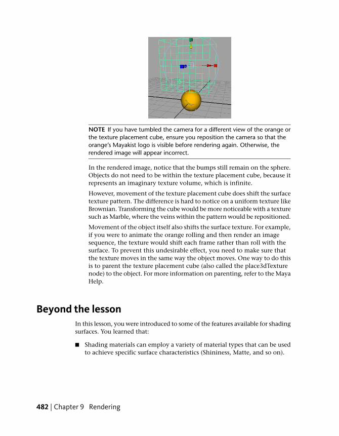
NOTE If you have tumbled the camera for a different view of the orange orthe texture placement cube, ensure you reposition the camera so that theorange’s Mayakist logo is visible before rendering again. Otherwise, therendered image will appear incorrect.
In the rendered image, notice that the bumps still remain on the sphere.Objects do not need to be within the texture placement cube, because itrepresents an imaginary texture volume, which is infinite.
However, movement of the texture placement cube does shift the surfacetexture pattern. The difference is hard to notice on a uniform texture likeBrownian. Transforming the cube would be more noticeable with a texturesuch as Marble, where the veins within the pattern would be repositioned.
Movement of the object itself also shifts the surface texture. For example,if you were to animate the orange rolling and then render an imagesequence, the texture would shift each frame rather than roll with thesurface. To prevent this undesirable effect, you need to make sure thatthe texture moves in the same way the object moves. One way to do thisis to parent the texture placement cube (also called the place3dTexturenode) to the object. For more information on parenting, refer to the MayaHelp.
Beyond the lessonIn this lesson, you were introduced to some of the features available for shadingsurfaces. You learned that:
■ Shading materials can employ a variety of material types that can be usedto achieve specific surface characteristics (Shininess, Matte, and so on).
482 | Chapter 9 Rendering
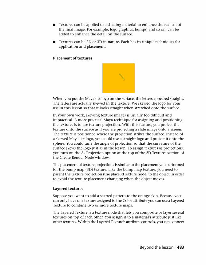
■ Textures can be applied to a shading material to enhance the realism ofthe final image. For example, logo graphics, bumps, and so on, can beadded to enhance the detail on the surface.
■ Textures can be 2D or 3D in nature. Each has its unique techniques forapplication and placement.
Placement of textures
When you put the Mayakist logo on the surface, the letters appeared straight.The letters are actually skewed in the texture. We skewed the logo for youruse in this lesson so that it looks straight when stretched onto the surface.
In your own work, skewing texture images is usually too difficult andimpractical. A more practical Maya technique for assigning and positioningfile textures is to use texture projection. With this feature, you project thetexture onto the surface as if you are projecting a slide image onto a screen.The texture is positioned where the projection strikes the surface. Instead ofa skewed Mayakist logo, you could use a straight logo and project it onto thesphere. You could tune the angle of projection so that the curvature of thesurface skews the logo just as in the lesson. To assign textures as projections,you turn on the As Projection option at the top of the 2D Textures section ofthe Create Render Node window.
The placement of texture projections is similar to the placement you performedfor the bump map (3D) texture. Like the bump map texture, you need toparent the texture projection (the place3dTexture node) to the object in orderto avoid the texture placement changing when the object moves.
Layered textures
Suppose you want to add a scarred pattern to the orange skin. Because youcan only have one texture assigned to the Color attribute you can use a LayeredTexture to combine two or more texture maps.
The Layered Texture is a texture node that lets you composite or layer severaltextures on top of each other. You assign it to a material’s attribute just likeother textures. Within the Layered Texture’s attribute controls, you can connect
Beyond the lesson | 483

other textures and control how they blend together. For example, the bottomlayer could be the logo image you used in the lesson, and a top layer couldbe an image of streaking lines that resemble scars. The combined logo andscars would give the orange the final aged look that you wanted.
Shader Library
As an option, you can install a Shader Library with Maya to help you quicklycreate common materials, such as bricks, fabrics, foods, and many other surfacetypes. When installed, a Shader Library tab appears in Hypershade. To use amaterial, find the type of shading you want, drag and drop it into Hypershade,then drag and drop it onto a surface in your scene using the middle mousebutton.
Lesson 3: Lights, shadows, and cameras
Introduction
Directors of live-action film use camera and lighting techniques to enhancethe visual impact of a scene. Wide, medium, and close up views of the subject,depth of field, high or low key lighting all communicate something about thesubject and the scene to the viewer.
484 | Chapter 9 Rendering
Lighting and camera techniques are one of the most crucial aspects to considerwhen working with artificial characters and objects. The more realistic thelighting and shading appear, the more convincing the scene will appear tothe viewer.
A prerequisite to creating effective 3D rendered animation is to study thelighting and camera effects used in live-action film. Your goal is to create thedesired scene ambience while keeping the lights and camera view asunobtrusive as possible.
In Maya, it is possible to simulate both realistic and unrealistic lighting andshadow effects for your final images and animations. In this lesson, you learnbasic techniques for working with lights, shadows, and cameras. In this lesson,you learn how to:
■ Create and position various types of lights in the scene.
■ Edit the attributes of lights and experiment with their effect in the scene.
■ Cast shadows on your surfaces using the lights and objects in the scene.
■ Create and animate an additional camera in the scene.
Open the scene for the lessonIn this lesson, you work with a scene we created for your use. In the first steps,you open the scene, create a directional light, and compare the directionallight’s effect to the scene’s default lighting.
1 Make sure you’ve done the steps in Preparing for the lessons on page 439.
2 Open the scene file named Lights.mb.
This file can be found in the GettingStarted directory that you set asyour Maya project:
GettingStarted\Rendering\Lights.mb
The scene contains a room with two walls and a floor. Sitting in the roomis a drafting table and lamp, grouped under the name tableGroup. Allobjects have a default gray shading.
Open the scene for the lesson | 485
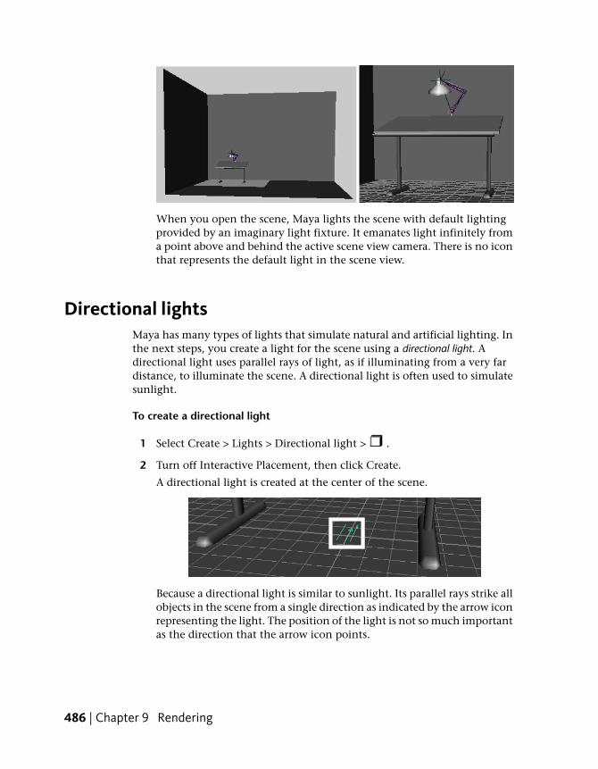
When you open the scene, Maya lights the scene with default lightingprovided by an imaginary light fixture. It emanates light infinitely froma point above and behind the active scene view camera. There is no iconthat represents the default light in the scene view.
Directional lightsMaya has many types of lights that simulate natural and artificial lighting. Inthe next steps, you create a light for the scene using a directional light. Adirectional light uses parallel rays of light, as if illuminating from a very fardistance, to illuminate the scene. A directional light is often used to simulatesunlight.
To create a directional light
1 Select Create > Lights > Directional light > .
2 Turn off Interactive Placement, then click Create.
A directional light is created at the center of the scene.
Because a directional light is similar to sunlight. Its parallel rays strike allobjects in the scene from a single direction as indicated by the arrow iconrepresenting the light. The position of the light is not so much importantas the direction that the arrow icon points.
486 | Chapter 9 Rendering
When you create a light, the scene view does not display its effect, bydefault. The scene view instead uses default lighting.
3 Select Lighting > Use All Lights (Hotkey: 7). This lights up the scene viewonly with lights you’ve created, not with default lighting. If you laterwant to see the scene view with default lighting again, select Lighting >Use Default Lighting (Hotkey: 6).
When you render the scene, by default, Maya uses all lights you’ve created.If you don’t create any lights, Maya creates a temporary default directionallight for you and then deletes it when the render is complete.
Next, you aim the directional light and edit its attributes.
To edit the directional light
1 With the directional light selected, rotate the light in various directions.The shading of surfaces changes as you rotate the light. The more directlythe light points at a surface, the brighter the shading. A directional lightis affected by its rotation, not its position. As you’ll see later, the positionof other lights affects the lighting.
2 Rotate the light as follows:
■ Rotate X: -40
■ Rotate Y: 25
■ Rotate Z: -20
With this orientation, all object surfaces in the scene show the effect ofthe light in the current camera view.
3 With the light still selected, open the Attribute Editor (under the Windowmenu). Drag the Intensity slider to various values to see the effects ofintensity.
Higher values brighten the surfaces. For example, an Intensity of 1.6brightens the lighting so much that the gray default shading of somesurfaces are bleached to white.
NOTE Several of the following illustrations in this lesson are snapshots of thescene after rendering. To render the scene, select Render > Render CurrentFrame. Do not use IPR rendering for this lesson because it doesn’tautomatically update the image for some of the changes you make to thescene.
Directional lights | 487

4 In the Attribute Editor, click the white Color box above the Intensitybox. This displays the Color Chooser.
5 Click inside the color wheel (hexagon) and drag the pointer to a red color.
The lighting imparts a red hue to the surfaces in the scene.
6 Change the color back to white and set the Intensity to 1.2 or so.
You’ll use these settings for the basic lighting of the scene.
SpotlightsIn the next steps, you light part of the desk by creating a spotlight andpositioning it within the desk lamp. A spotlight emits light from a single pointwithin a limited cone angle. You can aim a spot light in the direction youwant the light to illuminate.
To create a spotlight
1 Select Create > Lights > Spot Light > .
2 Turn off Interactive Placement, then click Create.
This creates the spotlight’s icon at the center of the grid. The light pointstoward the back wall.
3 Move the spotlight above the lamp. (Drag the light up along its localY-axis.)
488 | Chapter 9 Rendering

If you look at the spotlight icon from several angles, you’ll notice that itis shaped like a cone with an arrow pointing out of it.
The cone symbolizes that a spotlight emits a beam of light that graduallywidens with distance.
4 Select Modify > Transformation Tools > Show Manipulator Tool (seeModify > Transformation Tools > Move Tool, Rotate Tool, Scale Tool,Show Manipulator Tool).
With the spotlight selected, this tool provides two manipulators that youcan move to position and aim the light precisely.
The look-at point specifies where the light focuses. The eye point definesthe position of the light source. All types of lights have an eye point, butnot necessarily a look-at point.
5 Move the look-at point to the top of the table, and move the eye pointroughly to the center of the lamp housing.
Spotlights | 489

You can also use the Rotate tool to center the eye-point more accuratelyin the lamp housing.
An alternative way to position a spotlight is to select the light and thenselect Panels > Look Through Selected. You can then dolly and pan theview to focus on the desired surface. The area of focus is where the lightstrikes the surface. To return to the perspective view select Panels >Perspective > persp.
6 If you render the scene, you’ll notice that the spotlight lights up a circularregion on both the desk and the floor.
By default, light passes through and lights up each surface in its path.The circular region of light is wider on the floor than the desk because aspotlight emits a beam of light that widens with distance.
Only the floor, not the desk, will be lit by the spotlight in the scene view.You’ll see the desk lit up only if you render the scene.
7 You can prevent the light from passing through the table. With the lightselected, display the Attribute Editor. Open its Shadows section and thenthe Depth Map Shadow Attributes section, then turn on Use Depth MapShadows. Rendering creates this result:
490 | Chapter 9 Rendering

By turning on Use Depth Map Shadows, the spotlight’s lighting is blockedby the first surface it hits (the desk). The floor is in the shadow of thedesk so it receives no light. You’ll learn more about Depth Map Shadowslater in the lesson.
If you were to render the scene with IPR rather than the software renderer,the image would not automatically remove the lighting of the spotlightingfrom the floor when you turn on Use Depth Map Shadows. You wouldneed to refresh the image again in the Render View window by selectingIPR > Refresh IPR Image.)
Editing light attributesSpot lights, directional lights, and other light types have several uniqueattributes (for example, Intensity, Dropoff, Color, etc.). In the next steps, youmodify some of the attributes for the spotlight.
To modify the attributes of a spotlight
1 The spotlight’s default Cone Angle is 40 degrees. In the Attribute Editor,open the Spotlight Attributes section and set Cone Angle to 20.
The circle of light narrows.
2 Set Cone Angle to 60.
The circle of light widens. Rendering creates this result:
Editing light attributes | 491

3 Set Dropoff to 10.
This attribute sets how much the light intensity diminishes from thecenter of the circular region out to the edge. Finding the right value is amatter of experimentation. When you increase the Dropoff, the light’sintensity diminishes, so you need to increase the Intensity. For example,increase the Intensity to 1.6. Rendering creates this result:
To mimic the way a light source’s intensity naturally decreases withdistance, you might want to select a Decay Rate to diminish the light’sintensity. The Linear setting diminishes light with the least abruptness,Quadratic with the most abruptness. Cubic is between the two othersettings.
The default setting is No Decay, which means the light remains at fullintensity regardless of distance. If you use a setting other than No Decay,you likely will need to increase the Intensity. For this lesson, leave theDecay Rate set to No Decay.
4 Set the Penumbra Angle to 10.
This attribute controls the softness along the edge of the area ofillumination provided by the light. Again, finding the right value is amatter of experimentation. You can also use negative numbers to fade
492 | Chapter 9 Rendering
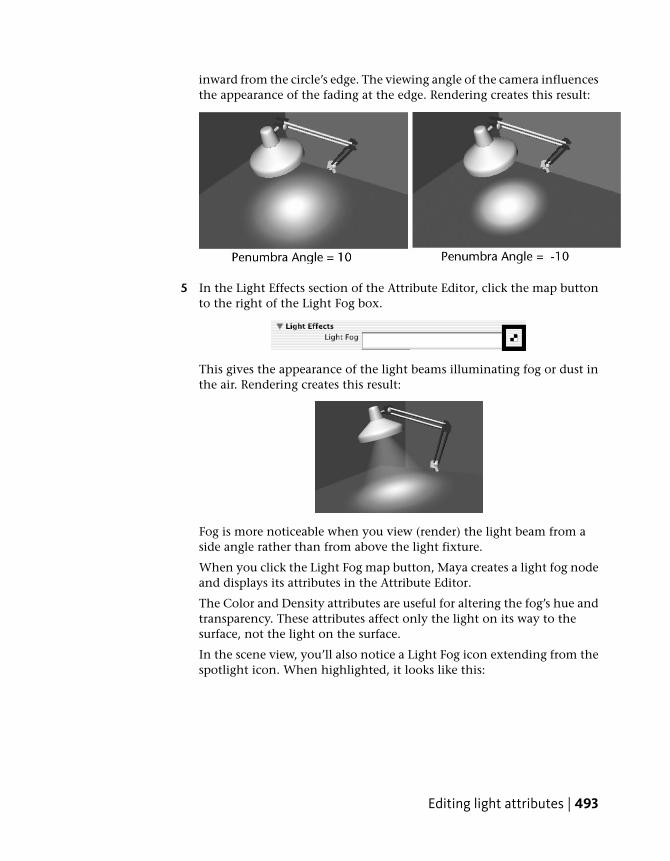
inward from the circle’s edge. The viewing angle of the camera influencesthe appearance of the fading at the edge. Rendering creates this result:
5 In the Light Effects section of the Attribute Editor, click the map buttonto the right of the Light Fog box.
This gives the appearance of the light beams illuminating fog or dust inthe air. Rendering creates this result:
Fog is more noticeable when you view (render) the light beam from aside angle rather than from above the light fixture.
When you click the Light Fog map button, Maya creates a light fog nodeand displays its attributes in the Attribute Editor.
The Color and Density attributes are useful for altering the fog’s hue andtransparency. These attributes affect only the light on its way to thesurface, not the light on the surface.
In the scene view, you’ll also notice a Light Fog icon extending from thespotlight icon. When highlighted, it looks like this:
Editing light attributes | 493

The icon displays the region of the potential illumination. You won’t seelight fog under the table. The table blocks the light fog because youpreviously turned on spotlight’s Depth Map Shadows attribute. You canuse the Scale tool on the icon to expand or contract the region of theillumination effect.
ShadowsShadows are the darkened areas that appear on a surface when an object getsin the path of a light source. Shadows are cast onto the area of a surface thatdoesn’t directly receive light. Shadows ground the objects in your scene andaid in defining their three-dimensional appearance. Shadows can add dramato your scene.
Next, you create a shadow on the floor from the light cast by the spotlight.To do this, you must edit a few of the spotlight’s attributes.
To create shadows using a spotlight
1 Select the spotlight and click the spotLightShape1 tab in the AttributeEditor.
2 Set the Cone Angle to 105.
When you render the scene, you’ll see the spotlight has widened its beamto light up a small part of the back wall. The table and light fixture blocklight and create shadows.
The shadows occur because you turned on Use Depth Map Shadows forthe spotlight earlier in the lesson.
494 | Chapter 9 Rendering
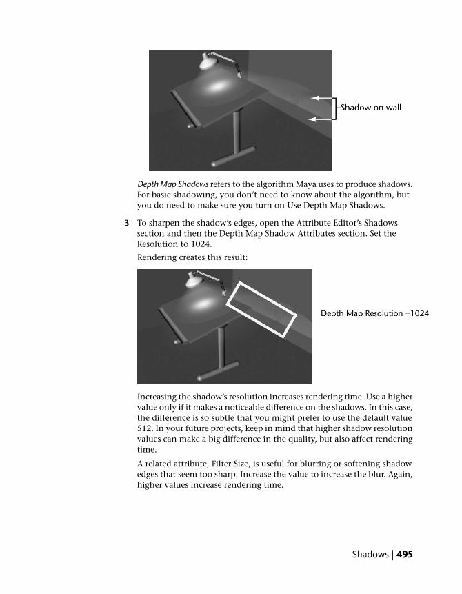
Depth Map Shadows refers to the algorithm Maya uses to produce shadows.For basic shadowing, you don’t need to know about the algorithm, butyou do need to make sure you turn on Use Depth Map Shadows.
3 To sharpen the shadow’s edges, open the Attribute Editor’s Shadowssection and then the Depth Map Shadow Attributes section. Set theResolution to 1024.
Rendering creates this result:
Increasing the shadow’s resolution increases rendering time. Use a highervalue only if it makes a noticeable difference on the shadows. In this case,the difference is so subtle that you might prefer to use the default value512. In your future projects, keep in mind that higher shadow resolutionvalues can make a big difference in the quality, but also affect renderingtime.
A related attribute, Filter Size, is useful for blurring or softening shadowedges that seem too sharp. Increase the value to increase the blur. Again,higher values increase rendering time.
Shadows | 495
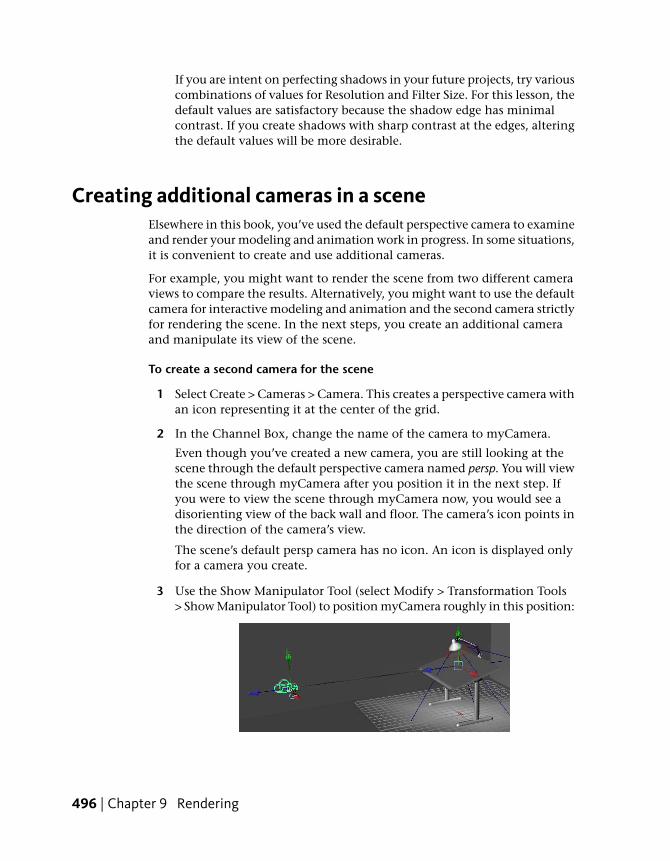
If you are intent on perfecting shadows in your future projects, try variouscombinations of values for Resolution and Filter Size. For this lesson, thedefault values are satisfactory because the shadow edge has minimalcontrast. If you create shadows with sharp contrast at the edges, alteringthe default values will be more desirable.
Creating additional cameras in a sceneElsewhere in this book, you’ve used the default perspective camera to examineand render your modeling and animation work in progress. In some situations,it is convenient to create and use additional cameras.
For example, you might want to render the scene from two different cameraviews to compare the results. Alternatively, you might want to use the defaultcamera for interactive modeling and animation and the second camera strictlyfor rendering the scene. In the next steps, you create an additional cameraand manipulate its view of the scene.
To create a second camera for the scene
1 Select Create > Cameras > Camera. This creates a perspective camera withan icon representing it at the center of the grid.
2 In the Channel Box, change the name of the camera to myCamera.
Even though you’ve created a new camera, you are still looking at thescene through the default perspective camera named persp. You will viewthe scene through myCamera after you position it in the next step. Ifyou were to view the scene through myCamera now, you would see adisorienting view of the back wall and floor. The camera’s icon points inthe direction of the camera’s view.
The scene’s default persp camera has no icon. An icon is displayed onlyfor a camera you create.
3 Use the Show Manipulator Tool (select Modify > Transformation Tools> Show Manipulator Tool) to position myCamera roughly in this position:
496 | Chapter 9 Rendering
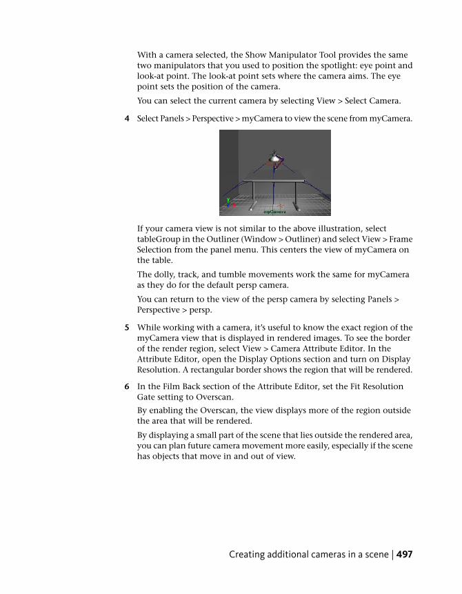
With a camera selected, the Show Manipulator Tool provides the sametwo manipulators that you used to position the spotlight: eye point andlook-at point. The look-at point sets where the camera aims. The eyepoint sets the position of the camera.
You can select the current camera by selecting View > Select Camera.
4 Select Panels > Perspective > myCamera to view the scene from myCamera.
If your camera view is not similar to the above illustration, selecttableGroup in the Outliner (Window > Outliner) and select View > FrameSelection from the panel menu. This centers the view of myCamera onthe table.
The dolly, track, and tumble movements work the same for myCameraas they do for the default persp camera.
You can return to the view of the persp camera by selecting Panels >Perspective > persp.
5 While working with a camera, it’s useful to know the exact region of themyCamera view that is displayed in rendered images. To see the borderof the render region, select View > Camera Attribute Editor. In theAttribute Editor, open the Display Options section and turn on DisplayResolution. A rectangular border shows the region that will be rendered.
6 In the Film Back section of the Attribute Editor, set the Fit ResolutionGate setting to Overscan.
By enabling the Overscan, the view displays more of the region outsidethe area that will be rendered.
By displaying a small part of the scene that lies outside the rendered area,you can plan future camera movement more easily, especially if the scenehas objects that move in and out of view.
Creating additional cameras in a scene | 497

Animating camera movesIn Maya, the camera can be animated. You can set keyframes for the cameramoves the same as for other objects in your scene. In the next steps, you setkeys to do a simple animation of the camera’s movement.
To animate the camera
1 Go to the start of the playback range.
2 Dolly, tumble, and track myCamera to create a view similar to this:
3 With myCamera selected, set a key for the camera’s current view at thefirst frame. To set a key, select the Animation menu set, and then selectAnimate > Set Key. (For details on setting keys and animation technique,see Lesson 1: Keyframes and the Graph Editor on page 200.)
TIP You can undo and redo view changes such as dolly, track, and tumbleby selecting either the [ or ] bracket respectively. You can press these keysrepeatedly to undo or return to a particular view orientation.
498 | Chapter 9 Rendering

4 Go to frame 150.
5 Dolly myCamera to create a view similar to this:
6 Set another key.
7 Play the animation to see the camera dolly toward the table for the first150 frames.
At this point, feel free to experiment with keying changes in the viewresulting from tumbling and tracking the camera. Excessive animationof tumbling and tracking creates a dizzying effect that is a commonmistake of inexperienced artists. In general, it’s best to keep cameraanimation simple except when you are striving for an unusual effect.
Beyond the lessonIn this lesson, you were introduced to some basic techniques related to lightsand cameras in Maya. You learned how to:
■ Place two types of lights in your scene and edit their attributes.In addition to the directional light and spotlight you created in this lesson,Maya has several other types of lights for creating nearly any type of naturalor artificial lighting. You might use as few as two lights or as many as 10to get the look you want. Generally, the more lights you create, the longerthe rendering will take.
In addition to the light fog effect you created in this lesson, you can alsocreate Glow, Halo, and Lens Flare light effects with a similar workflow. Tosee these effects, the light must point toward the camera view.
In some situations, you might want to prevent a light from striking asurface in its path. For example, your scene shows a person leaning againsta wall in an outdoor night setting. You might want to light the wall withdark, shadowy spotlights, and the person’s face only with a brighter, soft
Beyond the lesson | 499
spotlight. Because the face and the wall are near each other, all thespotlights currently strike both objects. You can use Maya’s light-linkingcapability to isolate the lighting.
■ Create shadows in the scene by having the lights cast shadows.The Maya software renderer has two types of shadows: Depth Map Shadowsand Ray Traced Shadows. In this lesson, you created Depth Map Shadows,which are less realistic than Ray Trace shadows but much faster to render.
Ray Traced Shadows are mainly useful in scenes where the audience isfocusing on the shadow region, for instance, a close-up of a still setting.Ray Traced Shadows are also useful if you want to cast shadows moreaccurately for transparent objects. To reduce rendering time, use Ray TracedShadows only when necessary.
■ Create and animate an additional camera from which to view the scene.If you have previous experience with photography, you’ll recognize thenames of various camera attributes displayed in the Attribute Editor whilea camera is selected. You can modify the attribute values to suit yourrequirements.
The values for certain camera attributes (for example, Film Aspect Ratio)might cause a rendered image to not match the region bounded by theResolution Gate. In such cases, you can display the Film Gate (View >Camera Settings > Film Gate) to see the region that will be rendered.
You can animate a camera along a path; for example, to create the illusionof flying through mountainous terrain. This type of animation involvesthe use of Animate > Motion Paths > Attach to Motion Path (from theAnimation menu set). If you additionally want the motion path-animatedcamera to focus on a stationary or moving object, you need to use Create> Cameras > Camera and Aim. If you want the camera to move in a loopingpath, (for example, a roller coaster) you need to use Create > Cameras >Camera, Aim, and Up.
Before you batch render a scene, you must select the camera you want touse for rendering. Select Window > Rendering Editors > Render Settingsto display the Render Settings window. In the File Output section, selectthe camera from the Camera option.
500 | Chapter 9 Rendering
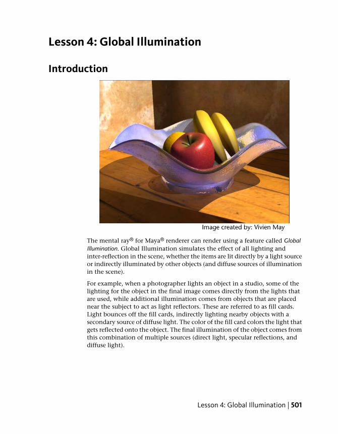
Lesson 4: Global Illumination
Introduction
The mental ray® for Maya® renderer can render using a feature called GlobalIllumination. Global Illumination simulates the effect of all lighting andinter-reflection in the scene, whether the items are lit directly by a light sourceor indirectly illuminated by other objects (and diffuse sources of illuminationin the scene).
For example, when a photographer lights an object in a studio, some of thelighting for the object in the final image comes directly from the lights thatare used, while additional illumination comes from objects that are placednear the subject to act as light reflectors. These are referred to as fill cards.Light bounces off the fill cards, indirectly lighting nearby objects with asecondary source of diffuse light. The color of the fill card colors the light thatgets reflected onto the object. The final illumination of the object comes fromthis combination of multiple sources (direct light, specular reflections, anddiffuse light).
Lesson 4: Global Illumination | 501
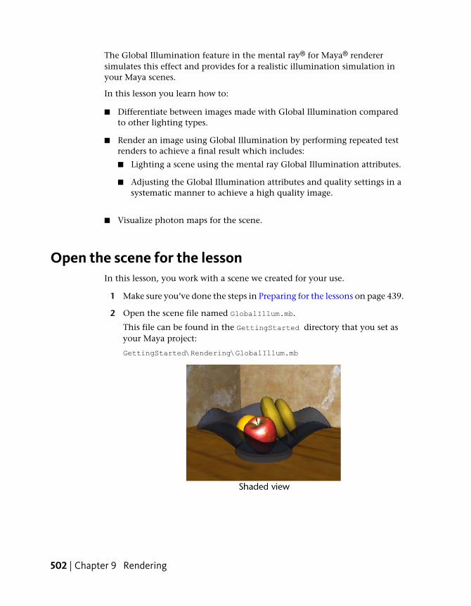
The Global Illumination feature in the mental ray® for Maya® renderersimulates this effect and provides for a realistic illumination simulation inyour Maya scenes.
In this lesson you learn how to:
■ Differentiate between images made with Global Illumination comparedto other lighting types.
■ Render an image using Global Illumination by performing repeated testrenders to achieve a final result which includes:
■ Lighting a scene using the mental ray Global Illumination attributes.
■ Adjusting the Global Illumination attributes and quality settings in asystematic manner to achieve a high quality image.
■ Visualize photon maps for the scene.
Open the scene for the lessonIn this lesson, you work with a scene we created for your use.
1 Make sure you’ve done the steps in Preparing for the lessons on page 439.
2 Open the scene file named GlobalIllum.mb.
This file can be found in the GettingStarted directory that you set asyour Maya project:
GettingStarted\Rendering\GlobalIllum.mb
502 | Chapter 9 Rendering
The scene contains a still life with a fruit bowl. Other surfaces act as the floorand walls for the scene. The primary light source is a spotlight. The spotlightcasts light through a vertical opening in the wall. Some areas in the scene aredirectly lit and other areas are not.
Shading materials have already been assigned to the bowl, fruit, and othersurfaces. The apple and orange models are from the previous lessons. If youwant to see what other shaders and textures are in the scene, you can viewthem by opening the Hypershade editor.
When you render this scene using Global Illumination, the effect you wantto achieve is to have the upper and lower regions of the scene receive indirectlight: you want to be able to view more detail in the shadow areas as a resultof the Global Illumination.
Render the scene using raytracingTo better understand the differences in a rendering performed using directlighting methods vs. global illumination, you begin by rendering the sceneusing the mental ray for Maya renderer without using Global Illumination.
You start by performing some preparatory setup and then render the scene.In this section you:
■ Select the mental ray for Maya renderer.
■ Set the quality setting for your rendering.
■ Set the image size for your rendering using the Image Size settings.When performing repeated test renders, a good practice is to render smallimages so the tests render quickly.
■ Turn on shadows for the spotlight in the scene.
■ Render an image using the mental ray for Maya renderer using raytracing.
Using the mental ray for Maya renderer
To use the Global Illumination feature in Maya you must render using themental ray for Maya renderer.
To render using the mental ray for Maya renderer you need to change therendering type from Maya to mental ray for Maya. You initially render thescene without using Global Illumination.
Render the scene using raytracing | 503

To change the renderer to mental ray for Maya
1 In the main menu, select Window > Rendering Editors > Render Settings(or click the Render Settings icon on the Status Line) to display the RenderSettings window.
2 In the Render Settings window, set the Render Using setting to mentalray.
When you render an image it will now use the mental ray for Mayarenderer.
NOTE When you switch between renderers in Maya (for example, MayaSoftware, Maya Hardware, and mental ray for Maya), the common RenderSettings do not require re-setting.
When you perform repeated test renderings for a particular scene, considerthe time it takes for each render to complete. If you reduce the time it takesto render each test image, the testing process proceeds much faster.
Setting render settings for raytracing
For the first rendering test, you render the scene to see how the scene appearswithout Global Illumination. The testing process proceeds faster if the qualitylevel for the image is initially set low.
To set presets for rendering
➤ At the top of the Render Settings window, select mental ray as yourrenderer. Click on the Quality tab and set the Quality Presets setting toDraft.
504 | Chapter 9 Rendering

The Draft setting ensures low anti-aliasing settings are used and reducesthe rendering time compared to other preset settings. This is a goodpractice when evaluating the lighting and basic material properties inyour test renderings.
Setting the image size for rendering
You set the size that an image is rendered in the Render Settings window. Forthis lesson, you render the image at a size that allows you to evaluate theGlobal Illumination effect.
To set the image size for rendering
1 At the top of the Render Settings window, select the Common tab andopen the Image Size settings.
2 Set the Preset to 320 X 240.
This sets a small image size for your rendering tests. The smaller imagesize renders in less time when compared to a larger image size.
3 Close the Render Settings window.
Render the scene using raytracing | 505
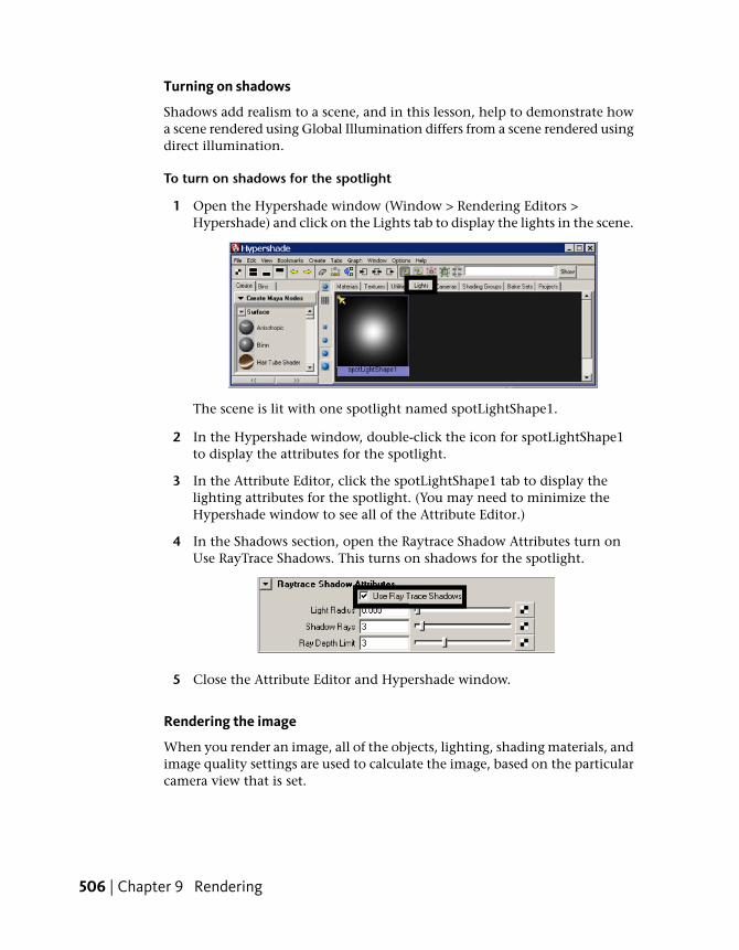
Turning on shadows
Shadows add realism to a scene, and in this lesson, help to demonstrate howa scene rendered using Global Illumination differs from a scene rendered usingdirect illumination.
To turn on shadows for the spotlight
1 Open the Hypershade window (Window > Rendering Editors >Hypershade) and click on the Lights tab to display the lights in the scene.
The scene is lit with one spotlight named spotLightShape1.
2 In the Hypershade window, double-click the icon for spotLightShape1to display the attributes for the spotlight.
3 In the Attribute Editor, click the spotLightShape1 tab to display thelighting attributes for the spotlight. (You may need to minimize theHypershade window to see all of the Attribute Editor.)
4 In the Shadows section, open the Raytrace Shadow Attributes turn onUse RayTrace Shadows. This turns on shadows for the spotlight.
5 Close the Attribute Editor and Hypershade window.
Rendering the image
When you render an image, all of the objects, lighting, shading materials, andimage quality settings are used to calculate the image, based on the particularcamera view that is set.
506 | Chapter 9 Rendering

To render an image using mental ray for Maya
1 Click in the perspective window. This indicates which camera view youwant Maya to render.
2 On the Status Line, click the Render Current Frame icon to launch therenderer to produce an image.
The Render View window appears and the fruit bowl scene renders usingthe mental ray for Maya renderer.
3 Once the render is complete, click the Keep Image icon in the RenderView window to save this image.
Keeping the image allows you to compare it to any subsequent test rendersyou produce. In this lesson you compare each rendered image to theprevious ones to understand how the changes you make in various settingsaffect the rendered image.
The rendered image shows the fruit bowl lit from the right of the frame.The upper and lower portions of the image are in shadow where the edgesof the wall prevented the spotlight from lighting those portions of thescene. The shadow areas appear dark and do not show any detail of thefloor or walls. This illumination effect is typical of an image producedwith a single light source and direct illumination.
Render the scene using raytracing | 507

Render the scene using Global IlluminationTo render using Global Illumination you need to turn on specific settings orattributes. There are two areas that you must initially set.
■ Turn on the Global Illumination rendering attributes using the RenderSettings Window.
■ Turn on the Global Illumination lighting attributes using the AttributeEditor.
You initially render the scene using the attributes at their default settings tosee how they affect the rendered image and then compare it to the previousraytrace rendering. As you gain more experience rendering with GlobalIllumination you will better understand what settings to initially use.
To turn on Global Illumination rendering attributes
1 Open the Render Settings window.
2 In the Render Settings window, click on the Quality tab and set theQuality Presets setting to Preview: Global Illumination.
This turns on preset attribute settings that enable and control the qualityof the Global Illumination. You initially render the scene using the defaultsettings. Once you’ve rendered an image and observed their effect, youreturn to the Render Settings window and modify the settings accordingly.
3 Close the Render Settings window.
Global Illumination uses photons to simulate the light inter-reflection effectsin a scene. Photons are small packets of energy emitted from a light sourceinto the scene that bounce off surfaces to determine the intensity of light forthose areas not receiving direct illumination. The renderer keeps track of theillumination that results from this photon emission in a file called a photonmap.
In addition to having the spotlight emit light you need to set the spotlight toalso emit photons for the Global Illumination simulation to occur. The overallillumination for the scene will be determined from a combination of the light’sintensity and photon illumination from this single spotlight.
508 | Chapter 9 Rendering

To turn on Global Illumination lighting attributes
1 Open the Hypershade window (Window > Rendering Editors >Hypershade) and click on the Lights tab to display the lights in the scene.
2 In the Hypershade, double-click on the icon for spotLightShape1 todisplay the attributes for the spotlight.
3 In the Attribute Editor, click the spotLightShape1 tab to display thelighting attributes for the spotlight.
4 Open the mental ray section, and in the Caustic and Global Illuminationattributes set the following settings:
■ Emit Photons: On
■ Photon Intensity: 8000
■ Global Illum Photons: 10000
The spotlight emits photons into the scene when you next render animage. Photon Intensity sets the brightness of the Global Illumination.Global Illum Photons sets the number of photons that get emitted intothe scene.
Setting a panel layout for rendering
The process of producing a rendered image usually involves rendering andevaluating successive test images to achieve the desired final image. Thisprocess involves adjusting many render quality, shading, and lighting settingsin specific windows and panels. Opening and closing the various windowscan become tedious.
Displaying the most frequently used windows and panels for rendering allowsyou to work more efficiently without having to open and close themrepeatedly.
To set a panel layout for rendering
1 Close the Render View window.
Render the scene using Global Illumination | 509

2 From the perspective view’s panel menu, select Panels > Saved Layouts> Hypershade/Render/Persp.
The panel layouts update to display the Hypershade window, RenderView window, and Perspective view simultaneously. This allows you toeasily work with these windows without having to open and close themrepeatedly.
If the image in the Render View window appears pixelated as a result ofthe new panel layout, do the following:
■ In the Render View window menu, select View > Real Size. This resizes therendered image to its actual size.
TIP You can resize the panels in a preset layout by dragging the borderbetween neighboring panels using your left mouse button.
Rendering the scene with Global Illumination
Now that the lights are set to emit photons and the Global Illumination presetis selected, you’re ready to render an a test image using Global Illumination.
To render the scene using Global Illumination
1 In the Render View window, click the Redo Previous Render icon to renderthe image with the default Global Illumination settings.
2 When the image has completed rendering, click the Keep Image icon tosave the image.
510 | Chapter 9 Rendering

3 Visually compare this rendered image with the previously renderedimages.
In this rendering, the shadow areas of the scene appear less dark as aresult of Global Illumination. The bowl also appears more transparentthan in the previous rendering.
The effect you want to achieve is to have the shadow regions receiveindirect light; that is, you want to be able to view more detail in theshadow areas as a result of the Global Illumination. To do this, you mustadjust the Global Illumination photon attributes. After you change anattribute, test render the scene to see the effect of this change in therendered image. These repeated test renderings or iterations allow you towork systematically towards the goal of creating the desired final image.
In the next steps you use the Attribute Editor to increase the Photon Intensityto increase the overall Global Illumination for the scene.
Increasing the brightness of Global Illumination
Increasing the Photon Intensity setting increases the brightness of GlobalIllumination. The goal is to provide more visible detail and brightness in theshadow areas of the scene in the next test image.
To increase the Global Illumination lighting
1 In the Hypershade window, double-click on the icon for spotLightShape1to display the attributes for the spotlight.
2 In the Attribute Editor, click the spotLightShape1 tab to display thelighting attributes for the spotlight.
Render the scene using Global Illumination | 511

3 In the Caustic and Global Illumination attributes adjust the settings tothe following:
■ Photon Intensity: 120000
Increasing the Photon Intensity increases the illumination in the areasaffected by Global Illumination.
To render the scene
1 In the Render View window, click the Redo Previous Render icon to renderthe image.
2 When the image has completed rendering, click the Keep Image icon tosave the image.
3 Compare this rendered image with the previously rendered images.
The brightness of the illumination in this image has increased as a resultof increasing the Photon Intensity. This is indicated by the increasedbrightness and details seen in the shadow areas of the scene. However,some circular spots have also appeared in the image along the dark wallbehind the bowl. These spots are the result of low photon quality settings.
Adjusting the quality of Global Illumination
The quality of Global Illumination is primarily affected by three attributes:
■ The accuracy of sampling (Accuracy)
■ The radius size that determines the size of the region surrounding aparticular sampling point (Radius).
■ The number of photons (Global Illum Photons).
512 | Chapter 9 Rendering

In the next steps, you return to the Render Settings window and the AttributeEditor to increase the quality attributes that affect the Global Illuminationeffect.
To increase the Global Illumination quality settings
1 In the Render Settings window, click on the Indirect Lighting tab andexpand the Global Illumination section. Change the following GlobalIllumination attributes to:
■ Accuracy: 900
■ Radius: 2.5
The Accuracy setting determines how many photons will be evaluated todetermine the Global Illumination intensity at a given sampling point.Radius determines the size of the region surrounding the particularsampling point. The more photons that get sampled, the more even theGlobal Illumination will appear in the final image.
NOTE As you increase the Global Illumination related quality and photonsettings, the time to render the image also increases. Your goal should be toincrease these settings just enough to achieve the desired image quality,without increasing them beyond what is required so that your renderingtimes are not adversely affected.
2 In the Render View window, click the Redo Previous Render icon to renderthe image.
3 When the image has completed rendering, click the Keep Image icon tosave the image and then compare this rendered image with the previouslyrendered images.
Render the scene using Global Illumination | 513

When the Accuracy and Radius values are increased, the resulting renderedimage shows the circular spots have almost fully disappeared and theGlobal Illumination is much more uniform when compared to theprevious rendering. Increasing the number of Global Illumination photonsshould aid in making the Global Illumination more uniform.
In the next steps, you increase the number of photons to provide a moreuniform Global Illumination in the scene.
To increase the Global Illumination photons
1 In the Hypershade, double-click on the icon for spotLightShape1 todisplay the attributes for the spotlight.
2 In the Attribute Editor, click the spotLightShape1 tab to display thelighting attributes for the spotlight.
3 In the Caustic and Global Illumination attributes adjust the settings tothe following:
■ Global Illum Photons: 80000
When you increase the number of Global Illumination Photons you areincreasing the resulting density of the photon map that gets producedat the beginning of the render process. The more photons, the smootherthe resulting Global Illumination. Increasing the number of photons alsoincreases the rendering time.
To render the image
1 In the Render View window, click the Redo Previous Render icon to renderthe image.
514 | Chapter 9 Rendering
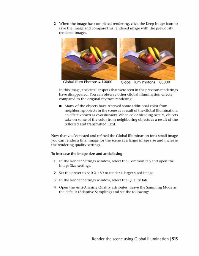
2 When the image has completed rendering, click the Keep Image icon tosave the image and compare this rendered image with the previouslyrendered images.
In this image, the circular spots that were seen in the previous renderingshave disappeared. You can observe other Global Illumination effectscompared to the original raytrace rendering:
■ Many of the objects have received some additional color fromneighboring objects in the scene as a result of the Global Illumination,an effect known as color bleeding. When color bleeding occurs, objectstake on some of the color from neighboring objects as a result of thereflected and transmitted light.
Now that you’ve tested and refined the Global Illumination for a small imageyou can render a final image for the scene at a larger image size and increasethe rendering quality settings.
To increase the image size and antialiasing
1 In the Render Settings window, select the Common tab and open theImage Size settings.
2 Set the preset to 640 X 480 to render a larger sized image.
3 In the Render Settings window, select the Quality tab.
4 Open the Anti-Aliasing Quality attributes. Leave the Sampling Mode asthe default (Adaptive Sampling) and set the following:
Render the scene using Global Illumination | 515

■ Number of Samples - Max sample level: 1
Sampling is the process for determining the amount of anti-aliasing thatoccurs. The Sample Level attribute sets minimum and maximum limitsfor the amount of sampling that will occur for a given pixel area in theimage. Modifying the anti-aliasing Sample Level settings will ensure thatthe surfaces in the rendered image appear smooth.
A Max value of 1 should provide the correct amount of anti-aliasingsampling for this particular image at this image size.
To render a final image of the scene
➤ In the Render View window, click the Redo Previous Render icon to renderthe image.
516 | Chapter 9 Rendering
Beyond the LessonIn this lesson you were introduced to the Global Illumination features providedby the mental ray® for Maya® renderer. You learned that:
■ The mental ray for Maya renderer provides a feature that simulates indirectillumination in the Maya scene called Global Illumination.
■ Global Illumination allows you to achieve realistic lighting effects forobjects and areas of the scene that do not receive direct lighting.
■ Photons are used to measure the Global Illumination of the scene via thecreation of a photon map.
■ The brightness of the Global Illumination in a scene is controlled by thePhoton Intensity.
■ The quality of the Global Illumination effect is dependent on the numberof photons emitted into the scene, the Accuracy, and the Radius attributesettings.
■ Multiple test renders are often required to achieve the desired final image.
Light sources for Global Illumination
Point, spot, and mental ray area lights can be used as light types for GlobalIllumination with the mental ray for Maya renderer. A Directional light doesnot work as a source for Global Illumination because this light type does nothave a defined point of origin (that is, the rays emit in a parallel manner).
Photon maps
You can visualize the photon mapping that occurs at the beginning of therendering process provided you turn on the Enable Map Visualizer option inthe Caustics and Global Illumination > Photon Tracing section of the RenderSettings window. To view a visualization of the photon mapping, selectWindow > Rendering Editors > mental ray > Map Visualizer.
Beyond the Lesson | 517
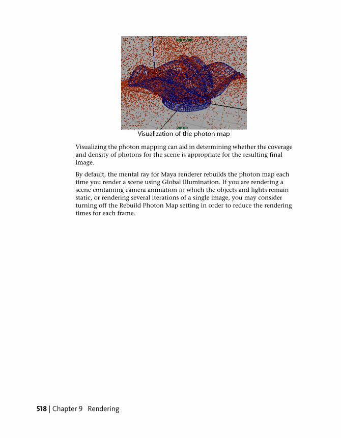
Visualizing the photon mapping can aid in determining whether the coverageand density of photons for the scene is appropriate for the resulting finalimage.
By default, the mental ray for Maya renderer rebuilds the photon map eachtime you render a scene using Global Illumination. If you are rendering ascene containing camera animation in which the objects and lights remainstatic, or rendering several iterations of a single image, you may considerturning off the Rebuild Photon Map setting in order to reduce the renderingtimes for each frame.
518 | Chapter 9 Rendering

Lesson 5: Caustics
Introduction
Caustics are the light effects and specular patterns that are cast on surfaces asa result of focused light reflecting off highly reflective surfaces or refractingthrough translucent surfaces.
The light patterns that occur on the bottom of a swimming pool on a sunnyday, or the bright areas that occur in the shadow of a glass object as lightshines through it are examples of caustics.
The Caustic feature in the mental ray® for Maya® renderer simulates causticeffects in your Maya scenes. Caustics are similar to Global Illumination in thatthey are an indirect illumination effect.
In this lesson you learn how to:
■ Create the shadow effect that results from the refraction and concentrationof light through a transparent object, using the Caustic feature providedin the mental ray for Maya renderer.
■ Adjust refraction level limits in order to achieve desired refractive effectswith transparent objects.
Lesson 5: Caustics | 519
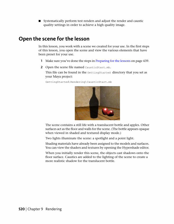
■ Systematically perform test renders and adjust the render and causticquality settings in order to achieve a high quality image.
Open the scene for the lessonIn this lesson, you work with a scene we created for your use. In the first stepsof this lesson, you open the scene and view the various elements that havebeen preset for your use.
1 Make sure you’ve done the steps in Preparing for the lessons on page 439.
2 Open the scene file named CausticStart.mb.
This file can be found in the GettingStarted directory that you set asyour Maya project:
GettingStarted\Rendering\CausticStart.mb
The scene contains a still life with a translucent bottle and apples. Othersurfaces act as the floor and walls for the scene. (The bottle appears opaquewhen viewed in shaded and textured display mode.)
Two lights illuminate the scene: a spotlight and a point light.
Shading materials have already been assigned to the models and surfaces.You can view the shaders and textures by opening the Hypershade editor.
When you initially render this scene, the objects cast shadows onto thefloor surface. Caustics are added to the lighting of the scene to create amore realistic shadow for the translucent bottle.
520 | Chapter 9 Rendering
Render the scene using raytracingTo better understand the differences between caustics versus other lighting,you begin by rendering the scene using the mental ray for Maya rendererwithout using Caustics.
You start by preparing the scene and then rendering. In this section you:
■ Set a panel layout for rendering
■ Turn on shadows for the spotlight
■ Turn on the mental ray for Maya renderer
■ Set the image size for your rendering
■ Set the image quality preset
■ Render the image using raytracing
Setting a panel layout for rendering
Producing a rendered image usually requires that you render test images toachieve the final result. This may involve adjusting many render quality,shading, and lighting settings. Opening and closing the various windows canbecome tedious.
Keeping the most frequently used windows and panels open allows you towork more efficiently.
In the following steps, you select a panel layout to work more efficiently withthe various panels and windows.
To set a panel layout for rendering
➤ From the perspective view’s panel menu, select Panels > Saved Layouts> Hypershade/Render/Persp.
Render the scene using raytracing | 521

The panel layouts update to display the Hypershade window, RenderView window, and Perspective view simultaneously.
When you render an image, it appears in the Render View window.
TIP You can resize the panels in a preset layout by dragging the borderbetween neighboring panels using your left mouse button.
Turning on shadows
In this lesson, you learn how the bottle’s shadow can be made to appear morerealistic as a result of the caustics.
To turn on shadows for the spotlight
1 In the Hypershade window, click the Lights tab.
The Hypershade displays icons for the two lights in the scene.
2 In the Hypershade window, double-click the icon for spotLightShape1.
The Attribute Editor appears.
3 In the Attribute Editor, click the spotLightShape1 tab to display thelighting attributes for the spotlight.
522 | Chapter 9 Rendering

4 In the Shadows section, open the Raytrace Shadow Attributes and turnon Use RayTrace Shadows.
When you render the scene, shadows are cast by the spotlight.
5 Hide the Attribute Editor by clicking the Show/Hide Attribute Editor iconon the Status Line.
Using the mental ray for Maya renderer
To use the Caustics feature in Maya you must render using the mental ray forMaya renderer.
To turn on the mental ray for Maya renderer
1 In the main menu, select Window > Rendering Editors > Render Settings(or click the Render Settings icon in the Render View window).
2 In the Render Settings window, set the Render Using setting to mentalray.
Render the scene using raytracing | 523

Setting the image size for rendering
You set the size that an image will be rendered in the Render Settings window.For this lesson, you render the image at a size that allows you to evaluate thecaustic effect.
To set the image size for rendering
1 At the top of the Render Settings window, select the Common tab andopen the Image Size settings.
2 Choose the 640 X 480 preset from the Presets drop-down list.
Setting render presets for raytracing
For the first rendering, you render the scene to see how the shadows appearwithout using caustics.
To set Render options for raytracing
1 In the Render Settings window, select the Quality tab and set the QualityPresets setting to Production.
The Production preset ensures that the refraction level settings (found inRaytracing Quality section) are at a level high enough to render objectswith translucency (for example, the bottle). The Production preset alsosets the anti-aliasing level for the image.
2 Close the Render Settings Window.
524 | Chapter 9 Rendering
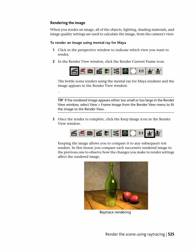
Rendering the image
When you render an image, all of the objects, lighting, shading materials, andimage quality settings are used to calculate the image, from the camera’s view.
To render an image using mental ray for Maya
1 Click in the perspective window to indicate which view you want torender.
2 In the Render View window, click the Render Current Frame icon.
The bottle scene renders using the mental ray for Maya renderer and theimage appears in the Render View window.
.
TIP If the rendered image appears either too small or too large in the RenderView window, select View > Frame Image from the Render View menu to fitthe image to the Render View.
3 Once the render is complete, click the Keep Image icon in the RenderView window.
Keeping the image allows you to compare it to any subsequent testrenders. In this lesson you compare each successive rendered image tothe previous one to observe how the changes you make to render settingsaffect the rendered image.
Render the scene using raytracing | 525
The rendered image shows the following:
■ A translucent bottle with apples beside it casting shadows towardsthe rear of the scene. Notice how the shadows appear when raytracerendered.
■ The distortion of the table surface in the translucent glass effect basedon the refractions and reflections.
■ A dark region on the surface of the bottle. This results from the bottlereflecting the empty black area of the scene in front of it.
In the next section, you turn on the caustics rendering attributes and renderthe scene.
Render the scene using causticsTo render using caustics you need to turn on specific settings or attributes.There are two sets of caustic-related attributes that you must initially set.
■ Turn on the caustics-related rendering attributes using the Render Settingswindow.
■ Turn on the caustics-related lighting attributes using the Attribute Editor.
You initially render the scene using these attributes at their default settingsto see how they affect the rendered image and then compare it to the previousraytrace rendering. As you gain more experience rendering with Caustics youwill better understand what settings to initially use.
To turn on the caustics preset settings
1 In the Render Settings window, select the Quality tab and set the Qualitypresets setting to PreviewCaustics.
This turns on the presets that control the quality of the caustics.
2 Close the Render Settings window.
Mental ray for Maya uses photons to simulate the caustic effects in a scene.Photons are small packets of energy emitted from a light source into the scene.The photons travel throughout the scene, refracting through transparentobjects or reflecting off reflective surfaces. The renderer keeps track of the
526 | Chapter 9 Rendering

illumination that results from this photon emission in a file called a photonmap. The overall caustic simulation is determined from the photon calculationsthat result.
In addition to having the spotlight emit light into the scene you set the lightto also emit caustic photons. The overall caustic effect is determined from thephoton calculations that result.
To turn on the caustics lighting settings
1 In the Hypershade, double-click on the icon for spotLightShape1.
2 In the Attribute Editor, click the spotLightShape1 tab to display thelighting attributes for the spotlight.
3 Open the mental ray section, and in the Caustic and Global Illuminationattributes set:
■ Emit Photons: On
■ Photon Intensity: 8000
■ Caustic Photons: 10000
4 Hide the Attribute Editor.
Rendering the scene with caustics
Now that the lights are set to emit caustic photons and the caustics preset isturned on, you’re ready to render an image using caustics.
Render the scene using caustics | 527

To render the scene using caustics
1 In the Render View window, click the Redo Previous Render icon.
2 When the image has completed rendering, click the Keep Image icon.
3 Compare this rendered image with the previously rendered image bydragging the scroll bar at the bottom of the Render View window left andright.
This image differs from the previous one in the following ways:
■ The bottle appears more opaque. This indicates that the correctnumber of refractions may not be occurring. The Raytracing RefractionLevel setting may need to be increased. When a different preset wasselected (Production to Preview), the refraction levels changed.
■ There are spotted areas on the table surface directly in front of thebottle. This can be corrected by adjusting the photon quality settings.
■ The desired caustic effect in the shadow has appeared but is not verypronounced. You want to achieve an effect where the shadow hasbrighter regions as a result of light being refracted through the surfacesof the bottle.
Adjusting the refraction levels
When the refraction levels are set too low, light rays do not refract throughall of the surfaces enough to provide a realistic indication of a translucentsurface when raytraced. This results in the object appearing opaque when itshould appear translucent.
528 | Chapter 9 Rendering
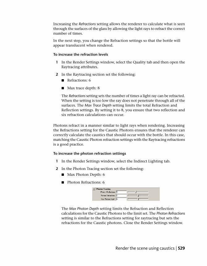
Increasing the Refractions setting allows the renderer to calculate what is seenthrough the surfaces of the glass by allowing the light rays to refract the correctnumber of times.
In the next step, you change the Refraction settings so that the bottle willappear translucent when rendered.
To increase the refraction levels
1 In the Render Settings window, select the Quality tab and then open theRaytracing attributes.
2 In the Raytracing section set the following:
■ Refractions: 6
■ Max trace depth: 8
The Refractions setting sets the number of times a light ray can be refracted.When the setting is too low the ray does not penetrate through all of thesurfaces. The Max Trace Depth setting limits the total Refraction andReflection settings. By setting it to 8, you ensure that two reflection andsix refraction calculations can occur.
Photons refract in a manner similar to light rays when rendering. Increasingthe Refractions setting for the Caustic Photons ensures that the renderer cancorrectly calculate the caustics that should occur with the bottle. In this case,matching the Caustic Photon refraction settings with the Raytracing refractionsis a good practice.
To increase the photon refraction settings
1 In the Render Settings window, select the Indirect Lighting tab.
2 In the Photon Tracing section set the following:
■ Max Photon Depth: 6
■ Photon Refractions: 6
The Max Photon Depth setting limits the Refraction and Reflectioncalculations for the Caustic Photons to the limit set. The Photon Refractionssetting is similar to the Refractions setting for raytracing but sets therefractions for the Caustic photons. Close the Render Settings window.
Render the scene using caustics | 529

Increasing the brightness of caustics
Increasing the Photon Intensity setting increases the brightness of the refractedcaustic that appears in the shadow of the bottle.
To increase the Photon Intensity
1 In the Hypershade window, double-click the icon for spotLightShape1to display the attributes for the spotlight.
2 In the Caustic and Global Illumination attributes for the light adjust thesettings to the following:
■ Photon Intensity: 36000
To render the scene
1 In the Render View window, click the Redo Previous Render icon to renderthe image.
2 Once the render is complete, click the Keep Image icon in the RenderView window to save this image.
3 Compare this rendered image with the previously rendered images.
The translucency of the glass now appears more realistic. The causticeffect is more evident in the shadow of the bottle. However, the spottedeffect, that appeared on the surface in front of the bottle, is morepronounced. These spots are the result of a low caustics quality setting.
Adjusting the quality of caustics
The quality of the caustic effects in a scene is primarily affected by the numberof photons, the accuracy of sampling, and the radius surrounding the sampled
530 | Chapter 9 Rendering

area of illumination. (If you have previously completed the Global Illuminationtutorial, you may notice similarities in this area.)
In the next steps, you return to the Render Settings window and the Attributeeditor to increase the quality attributes that affect the caustics effect.
To increase the caustics quality settings
1 In the Render Settings window, open the Caustics and Global Illuminationattributes and change the following Caustics attributes to:
■ Accuracy: 900
■ Radius: 1.5
The Accuracy determines how many photons will be evaluated todetermine the Caustic intensity at a given sampling point. Radiusdetermines the size of the region surrounding the particular samplingpoint. The more photons that get sampled, the more realistic the causticeffect appears in the final image.
2 Close the Render Settings window.
Increasing the number of caustic photons that get emitted into the scene alsoincreases the quality of the caustic effect. When you increase the number ofcaustic photons you increase the density of the resulting photon map thatgets produced at the beginning of the render process. The more photons, thesmoother the resulting caustics effect.
NOTE As you increase the caustic quality and photon settings so will the rendertime. Your goal should be to increase these settings just enough to achieve thedesired image quality, without increasing them beyond what is required so thatyour rendering times are not adversely affected. Performing test renderings is thebest method to determine these settings.
To increase the number of caustic photons
1 In the Hypershade window, double-click the icon for spotLightShape1.
Render the scene using caustics | 531

2 In the Caustic and Global Illumination attributes, adjust the followingsettings:
■ Caustic Photons: 50000
3 In the Render View window, click the Redo Previous Render icon.
4 When the image has completed rendering, click the Keep Image icon andcompare this rendered image with the previously rendered images.
In this image the bright spots in front of the bottle should be reducedwhen compared to the previous images. The caustic in the bottle’s shadowshould also appear more pronounced and more evenly illuminated.
Beyond the LessonIn this lesson you were introduced to the caustic features provided by themental ray® for Maya® renderer. You learned that:
■ Caustics provide additional realism in a rendered image by simulating thefocusing of light on diffuse surfaces as a result of the light reflecting offspecular surfaces or via the refraction of light through translucent surfaces.
■ Photons are used to determine the caustic effect in a scene via the creationof a photon map.
■ The brightness of the caustic is controlled by the Photon Intensity attribute.
532 | Chapter 9 Rendering

■ The quality of the caustic effect is controlled by the number of photonsemitted into the scene, the Accuracy, and the Radius attributes.
■ Multiple test renders are often required to achieve the desired final image.
Light sources for caustics
Point, spot, and mental ray area lights can be used as light types for causticswith the mental ray for Maya renderer. A Directional light does not work asa source for Caustics because this light type does not have a defined point oforigin (that is, the rays emit in a parallel manner).
Photon maps
You can visualize the photon mapping that occurs at the beginning of therendering process provided you turn on the Enable Map Visualizer option inthe Caustics and Global Illumination section of the Render Settings window.To view a visualization of the photon mapping, select Window > RenderingEditors > mental ray > Map Visualizer.
Visualizing the photon mapping can aid in determining whether the coverageand density of photons for the scene is appropriate for the resulting finalimage.
By default, the mental ray for Maya renderer rebuilds the photon map eachtime you render a scene using Caustics. If you are rendering a scene containingcamera animation in which the objects and lights remain static, or renderingseveral iterations of a single image, you may consider turning off the RebuildPhoton Map setting in order to reduce the rendering times for each frame.
Beyond the Lesson | 533

534
Dynamics
IntroductionDynamics is a branch of physics that describes how objects move using physicalrules to simulate the natural forces that act upon them. Dynamic simulationsare difficult to achieve with traditional keyframe animation techniques.
Maya provides a means to do this type of computer animation where you setup the conditions that you want to occur, then let the software solve how toanimate the objects in the scene. Maya® Dynamics™ provides the tools forcreating effects that will enhance your final images and animations.
With Particle Effects, you can create the illusions of smoke, fireworks, rain, fire,and explosions.
With Rigid Body Dynamics, you can simulate real-world physical interactionsbetween objects, such as collisions between surfaces. For example, you cansimulate a bowling ball crashing through pins or simulate the effects of gravitywhen a ball falls to the ground. You can also simulate natural forces, such aswind.
This chapter contains the following lessons:
■ Lesson 1 Particles, emitters, and fields: Introduction on page 536
■ Lesson 2 Rigid bodies and constraints: Introduction on page 554
Preparing for the lessonsDo these steps to ensure the lessons in this chapter work as described:
1 Select File > New Scene to create a new scene before you start each lesson.
10
535

2 If you have not already done so, copy the GettingStarted folder fromits installation location to your projects directory. Then, set theGettingStarted directory as your Maya project. For more information,see Copying and setting the Maya project on page 25.
3 Select Window > Settings/Preferences > Preferences. Click Timeline underCategories and make sure the Playback Speed is set to Play every frame.Dynamic animation plays more accurately with this setting.
4 Select the Dynamics menu set. Unless otherwise noted, the directions inthis chapter for making menu selections assume you’ve already selectedthe Dynamics menu set.
NOTE Before you perform the lessons in this book, ensure that the InteractiveCreation option for primitives is turned off by selecting Create > NURBSPrimitives > Interactive Creation. That is, ensure a check mark does not appearbeside the menu item.
Lesson 1: Particles, emitters, and fields
IntroductionParticles are points that display as dots, streaks, spheres, or other shapes.Particles can have attributes applied to them so they animate and render tosimulate natural phenomena.
You can create particles by clicking positions in the scene view, or you cancreate them with an emitter that shoots particles into view.
To animate particles, you typically apply fields such as gravity or wind. Bycombining emitters, particles, and fields, you can create natural phenomenasuch as smoke, fireworks, or rain.
In this lesson, you will be introduced to some of the basic concepts of particlesand use particles, emitters, and volume fields to create a fountain-like effect.In this lesson, you learn how to:
■ Create a particle emitter in your scene.
■ Create a field to direct the movement of particles.
■ Use a volume shape to control the movement of particles.
536 | Chapter 10 Dynamics

■ Work with particle attributes.
■ Color particles.
■ Use a color ramp to add colors to the particles.
■ Render the particles using hardware rendering.
Creating an emitterEmitters create particles as an animation plays. The emitter controls theposition, direction, quantity, and initial velocity of the emitted particles whenthey are born. After particles are born, the attributes of the particle objectcontrol their appearance.
You can make a standalone emitter, or you can make a surface, curve, andeven another particle an emitter. You move an emitter the same way youmove any geometry, such as setting keys or parenting it to a moving object.
In the next steps, you create a circle and emit particles from it.
To create a particle emitter
1 Make sure you’ve done the steps in Preparing for the lessons on page 535.
2 Set the start frame to 1 and end frame to 120.
3 Select Create > NURBS Primitives > Circle > . In the options window,set the following options and click Create:
■ Radius: 4
■ Number of Sections: 25
Creating an emitter | 537

With Radius set to 4, the circle will be wide enough to see the particleemission clearly. With Number of Sections set to 25, the emission willbe distributed evenly from points around the circle.
Note that the illustrations in this chapter show the grid with a customblue color and numbered lines so that the shape and size of the objectsyou create are easier to distinguish. (If you want to change the grid color
in your scene, select Display > Grid > .)
4 With the circle selected, select Particles > Emit from Object.
By default, this creates an Omni emitter. If you dolly toward the centerof the grid, you can see a tiny icon that represents the emitter. Whenyou create an Omni emitter on a NURBS object, for instance, a circle,each control vertex (CV) of the object emits particles in all directions.
5 Play the animation for a few seconds to see the emission.
The particles begin to emit from the object. When you create any typeof emitter, a particle object is automatically created and connected to it.
The connected particle object originally has no particles and is thereforeinvisible. As the animation plays and the emitter generates particles, theparticle count of the connected particle object increases. When you goto the start of the animation, the particle count returns to 0.
Note that if you had created the circle with a smaller Number of Sections,there would be fewer CVs for the circle and therefore bigger gaps betweenthe emission points on the circles.
538 | Chapter 10 Dynamics

6 Display the Outliner (Window > Outliner).
7 In the Outliner, select particle1.
This is the particle object. A particle object is a collection of particles thatshare the same attributes. You can create particle objects containing asingle particle or millions of particles. Each particle in a scene belongs tosome particle object.
The particle object’s attributes define the appearance and othercharacteristics of the emitted particles. The emitter’s attributes controlthe initial position, direction, quantity, and velocity of the emittedparticles.
Creating volume axis fieldsFields are forces that you use to animate the motion of particles. With a VolumeAxis field, you can move particles in various directions within the volume ofa cube, sphere, cylinder, cone, or torus. With clever use of this type of field,you can create effects such as particles flowing around obstacles, solar flares,explosions, tornadoes, and rocket exhaust.
In the next steps, you’ll use a volume axis field to move the particles up aconical path. When the particles exit the top of a conical region, you’ll useanother volume axis field to give them a downward arcing motion within atorus. The result resembles a fountain of light.
To create a cone volume axis field
1 With the particle object still selected, select Fields > Volume Axis > .
2 Set the following Volume Axis Options and click Create:
■ Magnitude: 50
■ Volume Shape: Cone
■ Away From Axis: 0
■ Along Axis: -1
NOTE If any of these options are not visible, enlarge the Volume AxisOptions window.
This creates a conical Volume Axis field that affects the motion of particlesthat enter or exist within its volume. Particles move in relation to a central
Creating volume axis fields | 539

axis within the volume. For a Cone Volume Shape, the central axis is thepositive Y axis:
Using the axis attributes, you can specify that the particles:
■ move in a direction roughly parallel to the axis toward or away from thepoint of the cone (Along Axis)
■ radiate outward or inward relative to the axis (Away From Axis)
■ swirl around the axis (Around Axis)
■ move in a direction based on a combination of these directionsBy setting Along Axis to -1, the particles move toward the point of thecone. (A positive value would move particles in the opposite direction.)In the next step, you’ll flip the cone 180 degrees so the aim of the coneand particles is upward.
By using 0 for the Away From Axis value rather than the default value of1, the particles will not radiate away from the axis.
Note that you can use larger or smaller values for the Axis attributes tointensify or diminish movement.
Magnitude specifies the strength of the volume axis field. The greater thevalue, the more force is exerted on the particles.
540 | Chapter 10 Dynamics
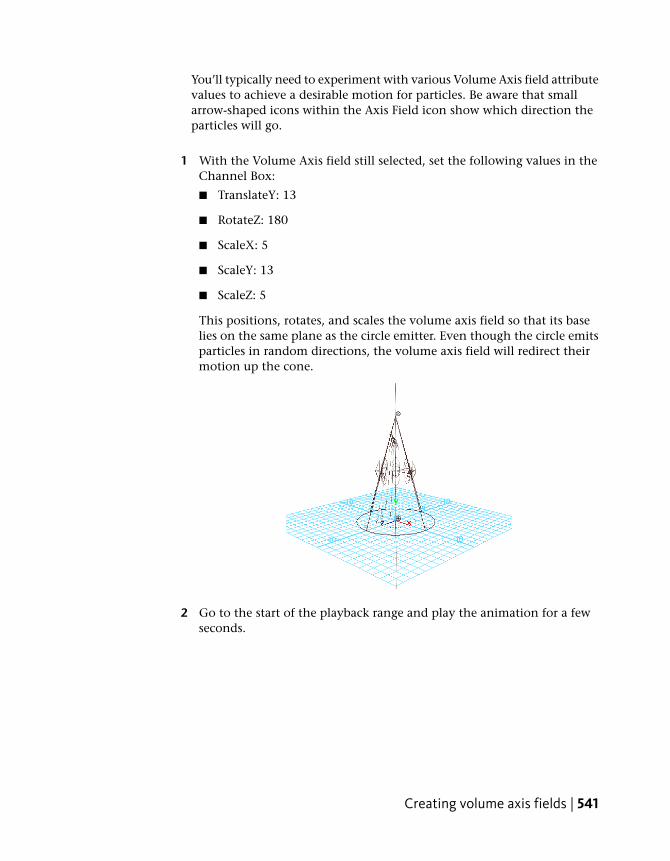
You’ll typically need to experiment with various Volume Axis field attributevalues to achieve a desirable motion for particles. Be aware that smallarrow-shaped icons within the Axis Field icon show which direction theparticles will go.
1 With the Volume Axis field still selected, set the following values in theChannel Box:
■ TranslateY: 13
■ RotateZ: 180
■ ScaleX: 5
■ ScaleY: 13
■ ScaleZ: 5
This positions, rotates, and scales the volume axis field so that its baselies on the same plane as the circle emitter. Even though the circle emitsparticles in random directions, the volume axis field will redirect theirmotion up the cone.
2 Go to the start of the playback range and play the animation for a fewseconds.
Creating volume axis fields | 541
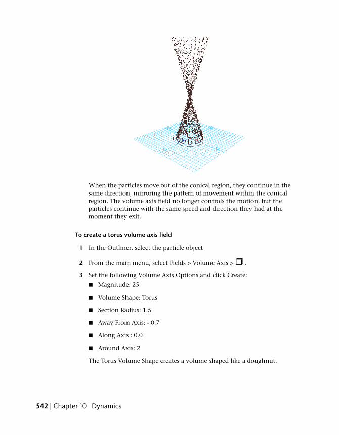
When the particles move out of the conical region, they continue in thesame direction, mirroring the pattern of movement within the conicalregion. The volume axis field no longer controls the motion, but theparticles continue with the same speed and direction they had at themoment they exit.
To create a torus volume axis field
1 In the Outliner, select the particle object
2 From the main menu, select Fields > Volume Axis > .
3 Set the following Volume Axis Options and click Create:
■ Magnitude: 25
■ Volume Shape: Torus
■ Section Radius: 1.5
■ Away From Axis: - 0.7
■ Along Axis : 0.0
■ Around Axis: 2
The Torus Volume Shape creates a volume shaped like a doughnut.
542 | Chapter 10 Dynamics

Section Radius defines the thickness of the torus.
A value of 2 for Around Axis causes the particles to swirl around thecentral axis. For a torus, the central axis is the ring in the center of thesolid part of the torus.
A value of -0.7 for Away From Axis causes the particles to move radiallytoward the central axis.
When you later play the animation, the combination of these valuescause the particles to loop up then down as if guided along the innerwalls of a torus.
Again, achieving the desired motion for particles within a volume axisfield requires experimentation with attribute values. Examine the arrows
Creating volume axis fields | 543

and other small icons within the axis volume field to help get the desiredresults.
Note that the field’s effect is pervasive enough that all particles passingthrough the hole of the torus are influenced by the field. You can causeparticles to pass through the hole by altering the Max Distance andAttenuation.
4 With the torus volume field still selected, enter the following values inthe Channel Box:
■ TranslateY: 15
■ ScaleX: 3.6
■ ScaleY: 3.6
■ ScaleZ: 3.6
This moves the torus volume field up 15 units and scales it larger. Findingthe appropriate position for the volume axis field is a matter ofexperimentation.
5 Go to the start of the playback range and play the animation.
When the particles move through the top of the cone region, they spreadoutward somewhat but do not follow the shape of the torus volume fieldas specified in the prior steps. You’ll correct this situation in the nextsteps.
544 | Chapter 10 Dynamics
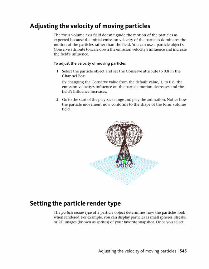
Adjusting the velocity of moving particlesThe torus volume axis field doesn’t guide the motion of the particles asexpected because the initial emission velocity of the particles dominates themotion of the particles rather than the field. You can use a particle object’sConserve attribute to scale down the emission velocity’s influence and increasethe field’s influence.
To adjust the velocity of moving particles
1 Select the particle object and set the Conserve attribute to 0.8 in theChannel Box.
By changing the Conserve value from the default value, 1, to 0.8, theemission velocity’s influence on the particle motion decreases and thefield’s influence increases.
2 Go to the start of the playback range and play the animation. Notice howthe particle movement now conforms to the shape of the torus volumefield.
Setting the particle render typeThe particle render type of a particle object determines how the particles lookwhen rendered. For example, you can display particles as small spheres, streaks,or 2D images (known as sprites) of your favorite snapshot. Once you select
Adjusting the velocity of moving particles | 545
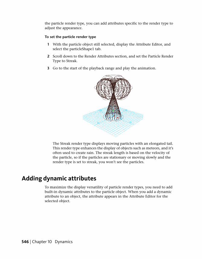
the particle render type, you can add attributes specific to the render type toadjust the appearance.
To set the particle render type
1 With the particle object still selected, display the Attribute Editor, andselect the particleShape1 tab.
2 Scroll down to the Render Attributes section, and set the Particle RenderType to Streak.
3 Go to the start of the playback range and play the animation.
The Streak render type displays moving particles with an elongated tail.This render type enhances the display of objects such as meteors, and it’soften used to create rain. The streak length is based on the velocity ofthe particle, so if the particles are stationary or moving slowly and therender type is set to streak, you won’t see the particles.
Adding dynamic attributesTo maximize the display versatility of particle render types, you need to addbuilt-in dynamic attributes to the particle object. When you add a dynamicattribute to an object, the attribute appears in the Attribute Editor for theselected object.
546 | Chapter 10 Dynamics

To add dynamic attributes
1 In the Attribute Editor, under the Render Attributes section, click theCurrent Render Type button next to Add Attributes.
2 Observe the attributes that are added.
3 Set the following attributes:
2Line Width This sets the width of eachstreak.
This sets the opacity of thetail fade; it can range from
0.5Tail Fade
0 to 1. A value of 1 makesthe tail completely opaque;a value of 0 makes the tailtransparent.
This scales the length of thetail. A value of 1 is the de-
2Tail Size
fault length. Values lessthan 1 shorten the tail; val-ues greater than 1 lengthenthe tail.
You can experiment with these settings to change the look of the particles.
Adding dynamic attributes | 547

Adding per particle attributesParticle objects have two different kinds of attributes: per object and perparticle.
A per object attribute lets you set the attribute value for all particles of theobject collectively with a single value. For instance, the per object colorattribute lets you set a single color for all the particles in the object.
A per particle attribute lets you set the value of the attribute individually foreach particle of the object. For example, the per particle rgbPP attribute letsyou set a unique color for each particle. Though there is only one rgbPPattribute in a particle object, the attribute holds the value for each particle’scolor value. The attribute holds the values in an array. An array is similar toa list. Arrays are appropriate for storing data which must be accessed in anunpredictable order, in contrast to lists which are best when accessedsequentially.
Although per particle attributes are best for creating complex effects, you can’tkeyframe them. You can keyframe per object attributes. In this lesson, youadd a per particle color attribute so you can give different particles differentcolors.
To add a per particle color attribute
1 In the Attribute Editor, expand the Add Dynamic Attributes section, ifnecessary.
2 Click the Color button. The Particle Color box is displayed,
3 Turn on the Add Per Particle Attribute and click Add Attribute. Noticethe rgbPP attribute that is added to the Per Particle (Array) Attributessection of the Attribute Editor.
548 | Chapter 10 Dynamics
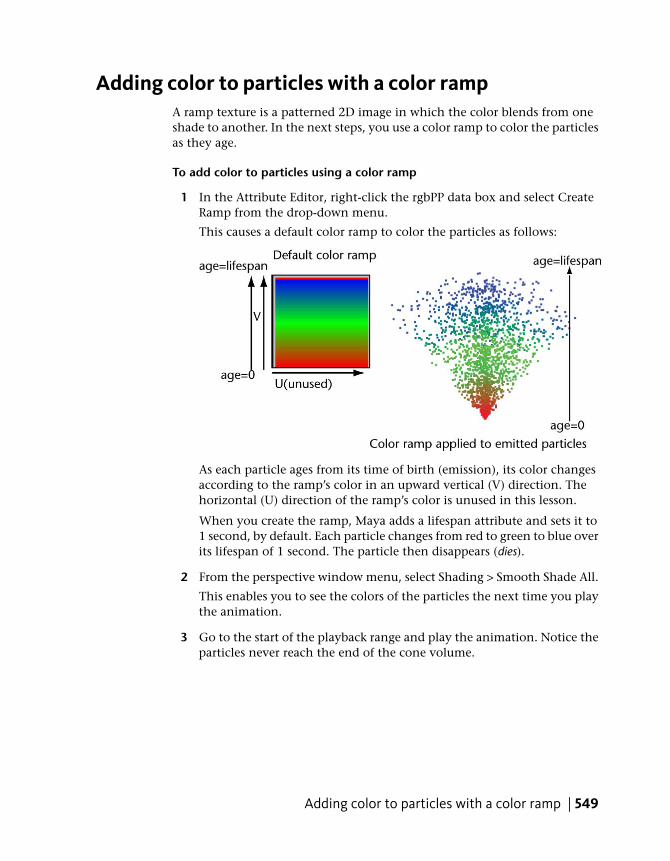
Adding color to particles with a color rampA ramp texture is a patterned 2D image in which the color blends from oneshade to another. In the next steps, you use a color ramp to color the particlesas they age.
To add color to particles using a color ramp
1 In the Attribute Editor, right-click the rgbPP data box and select CreateRamp from the drop-down menu.
This causes a default color ramp to color the particles as follows:
As each particle ages from its time of birth (emission), its color changesaccording to the ramp’s color in an upward vertical (V) direction. Thehorizontal (U) direction of the ramp’s color is unused in this lesson.
When you create the ramp, Maya adds a lifespan attribute and sets it to1 second, by default. Each particle changes from red to green to blue overits lifespan of 1 second. The particle then disappears (dies).
2 From the perspective window menu, select Shading > Smooth Shade All.
This enables you to see the colors of the particles the next time you playthe animation.
3 Go to the start of the playback range and play the animation. Notice theparticles never reach the end of the cone volume.
Adding color to particles with a color ramp | 549

This is because the Lifespan is set to the default of 1, which is the numberof seconds the particles exist in the animation.
4 In the Channel Box, set Lifespan to 3. Go to the start of the playbackrange and play the animation.
Because the particles live longer, they pass all the way through the coneand part of the way through the torus. The particles change from red togreen to blue and disappear as they are born, age, and die.
550 | Chapter 10 Dynamics
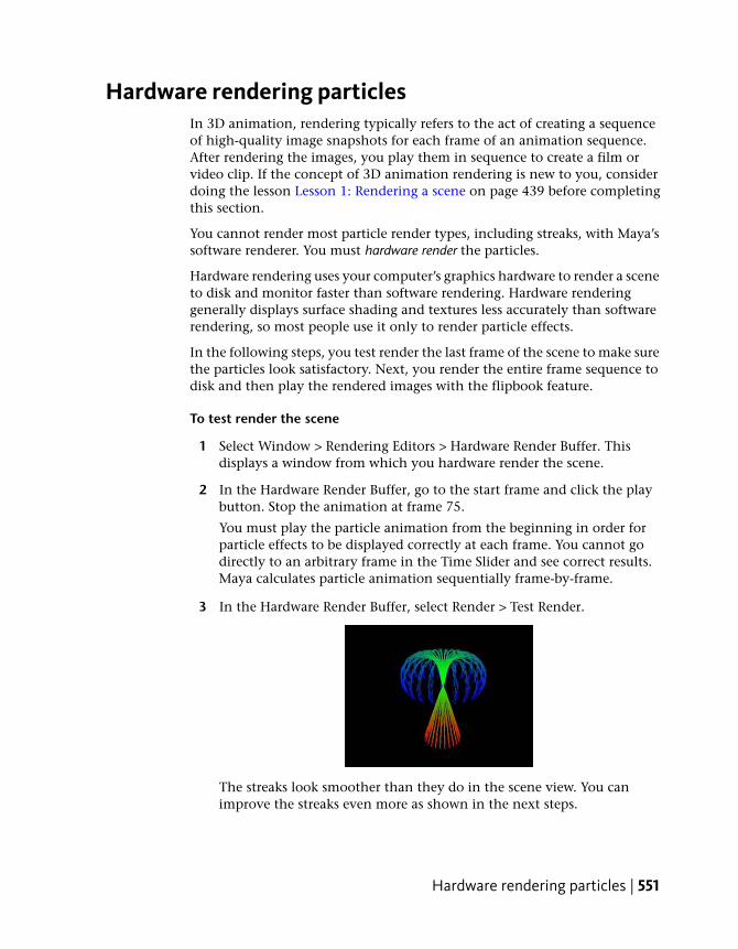
Hardware rendering particlesIn 3D animation, rendering typically refers to the act of creating a sequenceof high-quality image snapshots for each frame of an animation sequence.After rendering the images, you play them in sequence to create a film orvideo clip. If the concept of 3D animation rendering is new to you, considerdoing the lesson Lesson 1: Rendering a scene on page 439 before completingthis section.
You cannot render most particle render types, including streaks, with Maya’ssoftware renderer. You must hardware render the particles.
Hardware rendering uses your computer’s graphics hardware to render a sceneto disk and monitor faster than software rendering. Hardware renderinggenerally displays surface shading and textures less accurately than softwarerendering, so most people use it only to render particle effects.
In the following steps, you test render the last frame of the scene to make surethe particles look satisfactory. Next, you render the entire frame sequence todisk and then play the rendered images with the flipbook feature.
To test render the scene
1 Select Window > Rendering Editors > Hardware Render Buffer. Thisdisplays a window from which you hardware render the scene.
2 In the Hardware Render Buffer, go to the start frame and click the playbutton. Stop the animation at frame 75.
You must play the particle animation from the beginning in order forparticle effects to be displayed correctly at each frame. You cannot godirectly to an arbitrary frame in the Time Slider and see correct results.Maya calculates particle animation sequentially frame-by-frame.
3 In the Hardware Render Buffer, select Render > Test Render.
The streaks look smoother than they do in the scene view. You canimprove the streaks even more as shown in the next steps.
Hardware rendering particles | 551

4 In the Hardware Render Buffer window, select Render > Attributes.
The Attribute Editor appears.
5 In the Attribute Editor, under the Render Modes section, turn on LineSmoothing. This softens jagged edges when you hardware render Streakor MultiStreak render types.
6 To see the softened edges, select Render > Test Render.
If you click in the Hardware Render Buffer window, the rendered imagedisappears. If this occurs, select Render > Test Render again to redisplaythe image.
To render the sequence and playback the results
1 In the Hardware Render Buffer window, select Render > Attributes todisplay the Attribute Editor.
2 Set the Hardware Render Buffer settings as follows:
EmitFilename This name will be the baseof the filenames createdwhen you render all framesto images on disk.
This specifies the first frameof the animation sequenceto be hardware rendered.
1Start Frame
This specifies the last frameto be hardware rendered.
75End Frame
Other attributes in the Attribute Editor specify the image resolution, fileformat, lighting, and other display characteristics.
3 Make sure that no other windows overlap the Hardware Render Bufferor that your screensaver may accidentally launch while you use thisfeature. When you hardware render a frame sequence to disk, Mayarenders whatever exists within the borders of the Hardware Render Bufferwindow.
4 In the Hardware Render Buffer window, select Render > Render Sequence.
This creates a series of files named Emit.0001, Emit.0002, and so on,through Emit.0075. These files are the rendered frames 1 through 75.Maya puts the files in your current project’s images directory.
552 | Chapter 10 Dynamics
5 To play the hardware-rendered sequence, select Flipbooks > Emit.1-75.
6 Close the FCheck image viewing window when you are finishedexamining the animation.
Beyond the lessonIn this lesson you were introduced to a few of the basic concepts when usingparticles. You learned how to:
■ Create particles from a source object called an emitter.When you create any type of emitter, a particle object is also automaticallycreated and connected to it. Emitters can be points (CVs, vertices), surfaces(NURBS, polygons), curves (NURBS curves) or volumes (spheres, cylinders).
■ Control particles using fields, and volume objects.With volume axis fields, you can funnel or swirl particles within theboundaries of common volumetric shapes. Although this lesson showedhow to use a pair of volume axis fields to control the motion of particles,Maya has several other types of fields such as Gravity and Turbulence forsimulating natural phenomena. You can use the fields to animate themotion of curves and surfaces in addition to particles.
■ Change the color of particles using a ramp texture.You can also change ramp colors by editing other ramp attributes, such asNoise and Noise Frequency. To do so, right-click the attribute box for rgbPP,then select arrayMapper1.outColorPP > Edit Ramp. See the Maya Help fordetails on ramp attributes. You can also control other particle attributeswith ramps; for example, opacity. See the Maya Help for more information.
■ Render particles using the hardware renderer.The majority of particle rendering types are visible only when using thehardware render. Software rendering does not display them. However, ifyou use a particle render type of Blobby Surface, Cloud, or Tube, you mustrender the particles using the software renderer as hardware rendering doesnot display those types.
If you create a scene that includes both particles and geometric surfaces,you may need to render the scene twice, once with hardware renderingand once with software rendering. In such cases, you’ll need to compositethe two sets of rendered images using a compositing software package.
Beyond the lesson | 553

Lesson 2: Rigid bodies and constraints
IntroductionIn Maya, a rigid body is a surface which has the attributes of an unyieldingshape. Unlike conventional computer surfaces, rigid bodies collide rather thanpass through each other during animation and are used for creating dynamicsimulations. As well, rigid surfaces do not deform when they collide withother objects in Maya.
Rigid bodies can be created from polygonal or NURBS surfaces. Rigid bodyattributes can be assigned to the surfaces so they act and react in a simulationin specific ways. Examples of rigid body attributes are velocity, mass, andbounce.
To animate rigid body motion, you can use fields, keyframes, expressions,rigid body constraints, or collisions with particles or other rigid bodies.
Rigid body constraints restrict the motion of rigid bodies. The constraintssimulate the behavior of real-world items you’re familiar with, such as pins,nails, barriers, hinges, and springs.
In this lesson, you create a rigid body dynamic simulation in which you dropa ball on some planks and watch the simulation in action. In this lesson youlearn how to:
■ Create objects with physical properties.
■ Apply hinge constraints to objects so they react in specific ways.
■ Set attributes for the rigid bodies to be either active or passive for thesimulation.
■ Play back a rigid body dynamic simulation.
Lesson setupYou can create rigid bodies from NURBS surfaces and polygonal surfaces. Inthe following steps, you create some polygonal surfaces to be used for therigid bodies.
To create polygonal objects for the rigid body simulation
1 Make sure you’ve done the steps in Preparing for the lessons on page 535.
554 | Chapter 10 Dynamics
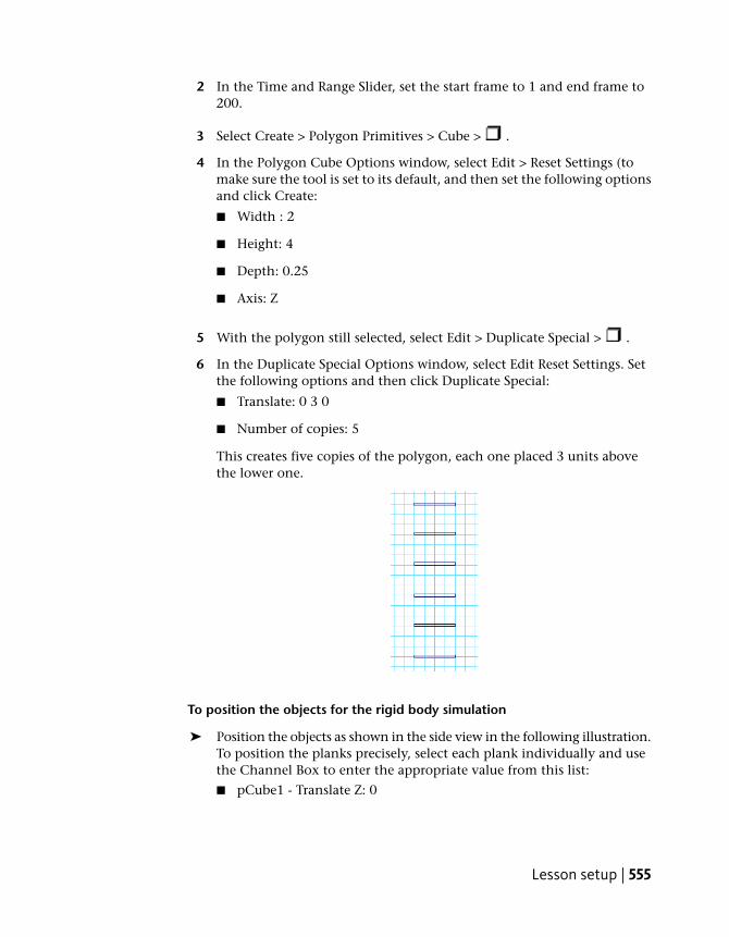
2 In the Time and Range Slider, set the start frame to 1 and end frame to200.
3 Select Create > Polygon Primitives > Cube > .
4 In the Polygon Cube Options window, select Edit > Reset Settings (tomake sure the tool is set to its default, and then set the following optionsand click Create:
■ Width : 2
■ Height: 4
■ Depth: 0.25
■ Axis: Z
5 With the polygon still selected, select Edit > Duplicate Special > .
6 In the Duplicate Special Options window, select Edit Reset Settings. Setthe following options and then click Duplicate Special:
■ Translate: 0 3 0
■ Number of copies: 5
This creates five copies of the polygon, each one placed 3 units abovethe lower one.
To position the objects for the rigid body simulation
➤ Position the objects as shown in the side view in the following illustration.To position the planks precisely, select each plank individually and usethe Channel Box to enter the appropriate value from this list:
■ pCube1 - Translate Z: 0
Lesson setup | 555
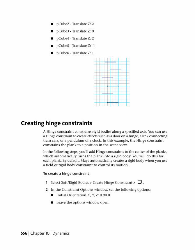
■ pCube2 - Translate Z: 2
■ pCube3 - Translate Z: 0
■ pCube4 - Translate Z: 2
■ pCube5 - Translate Z: -1
■ pCube6 - Translate Z: 1
Creating hinge constraintsA Hinge constraint constrains rigid bodies along a specified axis. You can usea Hinge constraint to create effects such as a door on a hinge, a link connectingtrain cars, or a pendulum of a clock. In this example, the Hinge constraintconstrains the plank to a position in the scene view.
In the following steps, you’ll add Hinge constraints to the center of the planks,which automatically turns the plank into a rigid body. You will do this foreach plank. By default, Maya automatically creates a rigid body when you usea field or rigid body constraint to control its motion.
To create a hinge constraint
1 Select Soft/Rigid Bodies > Create Hinge Constraint > .
2 In the Constraint Options window, set the following options:
■ Initial Orientation X, Y, Z: 0 90 0
■ Leave the options window open.
556 | Chapter 10 Dynamics
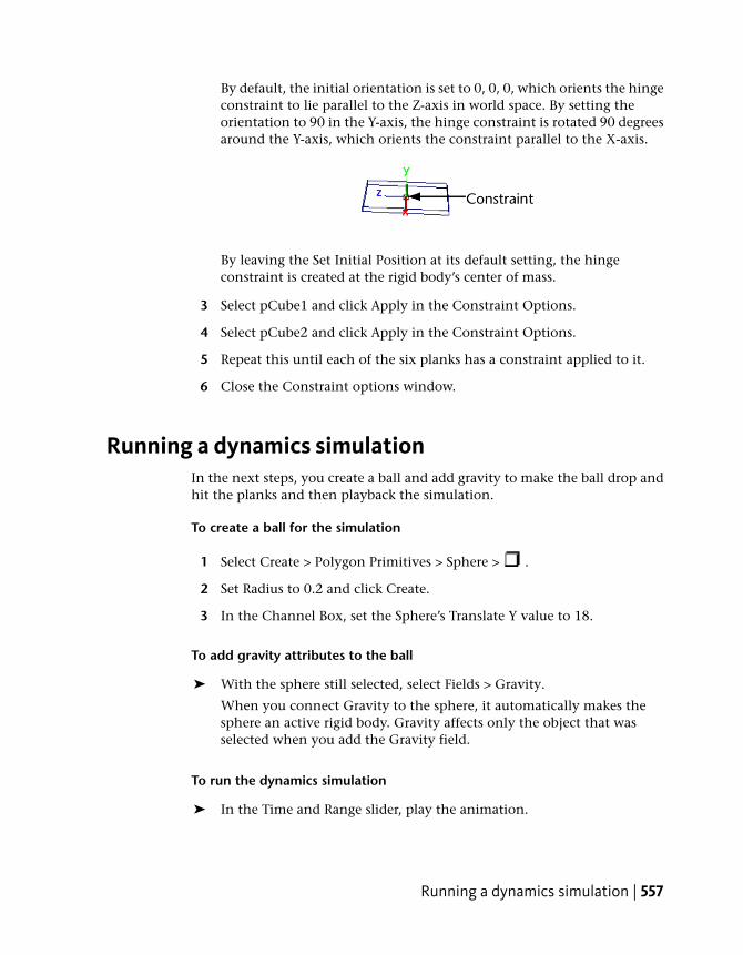
By default, the initial orientation is set to 0, 0, 0, which orients the hingeconstraint to lie parallel to the Z-axis in world space. By setting theorientation to 90 in the Y-axis, the hinge constraint is rotated 90 degreesaround the Y-axis, which orients the constraint parallel to the X-axis.
By leaving the Set Initial Position at its default setting, the hingeconstraint is created at the rigid body’s center of mass.
3 Select pCube1 and click Apply in the Constraint Options.
4 Select pCube2 and click Apply in the Constraint Options.
5 Repeat this until each of the six planks has a constraint applied to it.
6 Close the Constraint options window.
Running a dynamics simulationIn the next steps, you create a ball and add gravity to make the ball drop andhit the planks and then playback the simulation.
To create a ball for the simulation
1 Select Create > Polygon Primitives > Sphere > .
2 Set Radius to 0.2 and click Create.
3 In the Channel Box, set the Sphere’s Translate Y value to 18.
To add gravity attributes to the ball
➤ With the sphere still selected, select Fields > Gravity.
When you connect Gravity to the sphere, it automatically makes thesphere an active rigid body. Gravity affects only the object that wasselected when you add the Gravity field.
To run the dynamics simulation
➤ In the Time and Range slider, play the animation.
Running a dynamics simulation | 557
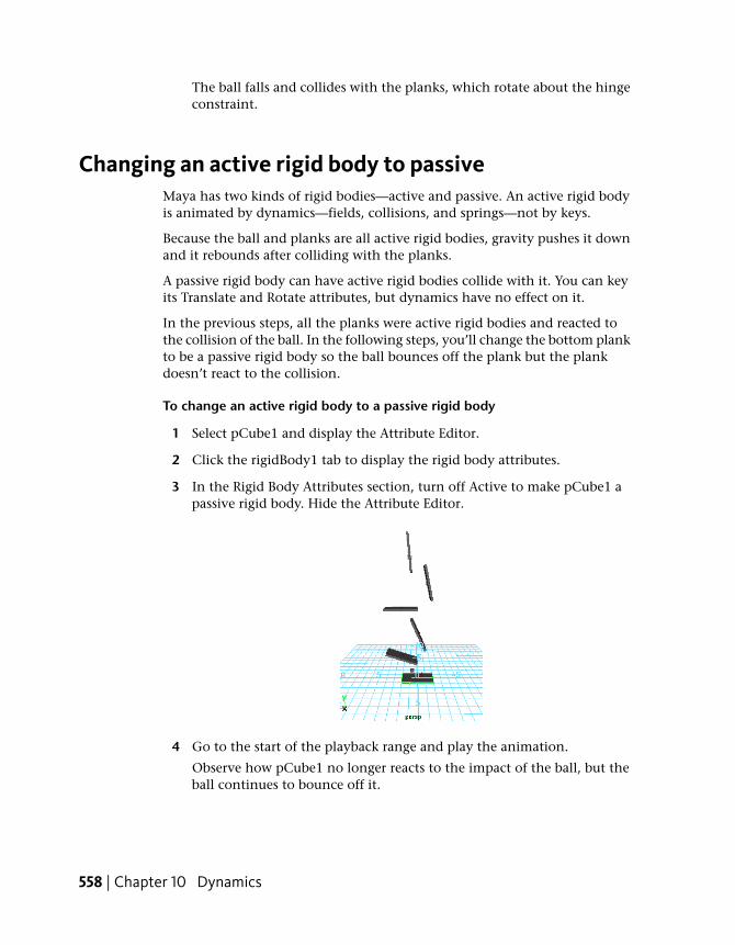
The ball falls and collides with the planks, which rotate about the hingeconstraint.
Changing an active rigid body to passiveMaya has two kinds of rigid bodies—active and passive. An active rigid bodyis animated by dynamics—fields, collisions, and springs—not by keys.
Because the ball and planks are all active rigid bodies, gravity pushes it downand it rebounds after colliding with the planks.
A passive rigid body can have active rigid bodies collide with it. You can keyits Translate and Rotate attributes, but dynamics have no effect on it.
In the previous steps, all the planks were active rigid bodies and reacted tothe collision of the ball. In the following steps, you’ll change the bottom plankto be a passive rigid body so the ball bounces off the plank but the plankdoesn’t react to the collision.
To change an active rigid body to a passive rigid body
1 Select pCube1 and display the Attribute Editor.
2 Click the rigidBody1 tab to display the rigid body attributes.
3 In the Rigid Body Attributes section, turn off Active to make pCube1 apassive rigid body. Hide the Attribute Editor.
4 Go to the start of the playback range and play the animation.
Observe how pCube1 no longer reacts to the impact of the ball, but theball continues to bounce off it.
558 | Chapter 10 Dynamics

Beyond the lessonIn this lesson you learned some fundamental concepts with respect to rigidbody dynamics.
■ There are differences between active and passive rigid bodies.When a rigid body is passive, active rigid bodies can collide with it butwill not move it. You can control its movement by setting keys.
When a rigid body is active, you control its movement using dynamicforces, specifically fields and collisions. You can change the active andpassive state of the rigid body to achieve various effects. For example, youcan roll a ball off a table using keys (passive rigid body) then cause the ballto fall using gravity (active rigid body).
■ A hinge constraint can be used between an active rigid body and a positionin the scene view.You can also create a hinge constraint between a passive rigid body and aposition in the scene view, two rigid bodies, and an active and passiverigid body.
Other types of constraints include pin, nail, spring and barrier constraints.For additional information on the types of constraints and their usage,please refer to the Maya Help.
Beyond the lesson | 559

560

Painting
Introduction
Maya provides painting tools that go above and beyond what many 3D creativeartists might normally envision. These tools allow you to accomplish a widerange of modeling, animation, texturing, and effects work.
The painting tools are separated into three categories: Maya® Artisan™ brushtools, Maya® Paint Effects™ tools, and 3D Paint. If you completed the previouslessons in Getting Started with Maya, you already have experience with a fewof these tools.
The Artisan brush tools have a variety of applications and allow you to directlymodify attribute values interactively:
■ In the NURBS modeling lesson, you used the brush tools to sculpt a simpleface from a sphere.
11
561
■ In the Character Setup chapter, you used Artisan brush tools to modifythe skin weights on a surface mesh to ensure the character’s joint deformedproperly.
■ In the Character Setup chapter, you used the Artisan brush tools to modifythe cluster weights for Control Vertices to ensure a blend shape deformerworked predictably.
As you have seen, Artisan brush tools can also be used to select surfacecomponents. This selection method can dramatically improve the speed ofyour workflow.
Maya Paint Effects allows the user to create natural and fantastic effects eitheron a 2D canvas or as actual 3D objects in the scene.
■ Paint Effects enables you to create a 2D backdrop for your scene, or adynamic 3D paint effect such as a field of grass, with flowers and awind-blown tree—all at the drag of your mouse or tablet pen.
■ Paint Effects comes with a suite of preset brushes to enable you to createmany types of 2D and 3D effects.
With 3D paint, you can paint and modify textures directly onto 3D surfacesusing both the Artisan and Paint Effects tools. You can paint texture attributessuch as color, transparency, and bump, to name but a few.
As you have already gained some experience with the Artisan brush tools, thischapter focuses on Paint Effects and 3D Paint. It includes the following lessons:
■ Lesson 1 Painting in 2D using Paint Effects: Introduction on page 563
■ Lesson 2 Painting in 3D using Paint Effects: Introduction on page 575
■ Lesson 3 Painting textures on surfaces: Introduction on page 608
Preparing for the lessonsTo ensure the lessons work as described, do the following:
1 Consider doing the lessons in the Rendering section of this guide.Familiarity with Maya rendering concepts is important to understandingthe following lessons.
2 If you have not already done so, copy the GettingStarted folder fromits installation location to your projects directory. Then, set the
562 | Chapter 11 Painting

GettingStarted directory as your Maya project. For more information,see Copying and setting the Maya project on page 25.
3 Select File > New Scene to create a new scene.
4 To use all available screen space, maximize the Maya window.
5 From a panel menu bar, select Panels > Layouts > Single Pane.
6 Select the Rendering menu set. Unless otherwise noted, the directions inthis chapter assume the Rendering menu set is selected.
Lesson 1: Painting in 2D using Paint Effects
IntroductionOne of the features of the Paint Effects Tool is the ability to paint colors,patterns, and textures on a 2D canvas image. You can use the image as anindependent piece of art, a background image in your scene, or a texture tobe applied to a 3D surface.
In this lesson, you learn how to:
■ Display the 2D canvas.
■ Paint strokes on the canvas, and modify your paint brush.
■ Use the Visor to access the many pre-defined paint brushes.
■ Modify brush settings such as brush size, color, and transparency.
■ Modify the canvas size.
■ Smear, blur, and erase brush strokes from the 2D canvas.
■ Use the pre-defined Paint Effects brushes to paint flowers and foliage.
■ Save modified brush settings to the Shelf.
■ View the alpha channel for your 2D image.
Lesson 1: Painting in 2D using Paint Effects | 563

Painting strokesIn the following steps, you display the 2D canvas and use preset brushes topaint a few strokes.
Although not covered in this lesson, you can use a tablet and stylus to paintwith pressure sensitivity. The harder you press down, the more paint is applied.
To paint strokes on the 2D canvas
1 Do the steps in Preparing for the lessons on page 562.
2 If you want to create maximum space in the Maya window, turn offDisplay > UI Elements > Channel Box/Layer Editor, Tool Settings, andAttribute Editor.
3 On the panel menu bar, select Panels > Panel > Paint Effects (hotkey 8).
The panel displays a Paint Effects toolbar and menus.
4 From the Paint Effects menus, select Paint > Paint Canvas to display the2D canvas.
You’re ready to start painting. It is not possible to display a grid on thecanvas.
5 Paint a stroke by dragging across the canvas.
When you first display the Paint Effects panel, your strokes use the defaultbrush—a solid black stroke similar to an airbrush.
564 | Chapter 11 Painting

TIP You can dolly and track the canvas using Maya’s standard mouse andkeyboard conventions.
6 Now paint with various preset brushes. To select a preset brush, selectBrush > Get Brush or click the following button in the toolbar:
The Visor window opens.
The Visor organizes the hundreds of Paint Effects brushes into category folders.In the Visor, click a folder, then click a brush icon in the area to the right ofthe folders. (The name of each preset brush has the extension .mel becauseeach is a MEL script that establishes the brush’s operation characteristics.) Youcan dolly within the Visor window to enlarge the viewable size of the brushicons and read the names more clearly.
You can copy a brush or all brushes within a folder to the Shelf. Use the middlemouse button to drag the brush or folder to the Shelf. Use the shelf editor(available from the arrow menu at the left of the shelf) to remove items fromthe shelf.
Some brushes apply paint directly along the paint path, while others produceadded effects. For example, the pens folder includes brushes such asballpointRed.mel that work like pens, while the flowers folder includes brushessuch as dahliaPink.mel that grow flowers as you drag the mouse. Brushes likedahliaPink.mel use Paint Effects tubes.
1 Select the dahliaPink.mel brush and drag the mouse slowly for one stroke,then quickly for the next stroke.
Painting strokes | 565

When you paint a stroke slowly, the density of flowers is higher thanwhen you paint quickly. The effect of stroke speed on density works thesame for all brushes that use tubes.
2 To erase your last stroke, select Canvas > Canvas Undo.
When displaying the 2D canvas, you can undo only a single stroke. Edit> Undo, Redo, Repeat (on the main menu) doesn’t undo strokes.
3 To erase the entire canvas, select Canvas > Clear or click the Canvas Clear
button on the toolbar:
Modifying the default brush settingsWhen you select a preset brush, Maya copies its brush settings to a templatebrush. A template brush is a holder for the attribute settings of the next strokesyou paint. When you change the settings of the template brush, they affectonly the next strokes, not previous strokes.
To edit the template brush settings
1 Select Brush > Reset Template Brush to select the default brush, thenpaint on the canvas so you remember the brush effect.
2 Select Brush > Edit Template Brush or click the following button in the
toolbar:
You can edit various brush settings, for example, the brush width, in thewindow that appears.
3 To resize the brush, change the Global Scale value. Alternatively, you canmove the brush over the canvas, press and hold the b Hotkey and dragleft or right. The circle on the canvas represents the size of your brush.
4 Paint on the canvas to try out a new size.
566 | Chapter 11 Painting

5 Close the Paint Effects Brush Settings window.
6 On the toolbar, click the swatch to the right of C (color) to display theColor Chooser.
7 Select a color from the Color Chooser and paint on the canvas.
8 On the toolbar, slide the T (transparency) slider to the right until the Tbox is a light gray. Paint on the canvas.
When you paint over existing paint strokes you will notice that yourpaint is transparent allowing the previous strokes to show through.
NOTE The Toolbar color boxes, for example, C and T, are also available inthe Paint Effects Brush Settings window. (Select Brush > Edit Template Brush> Shading.)
Modifying the default brush settings | 567
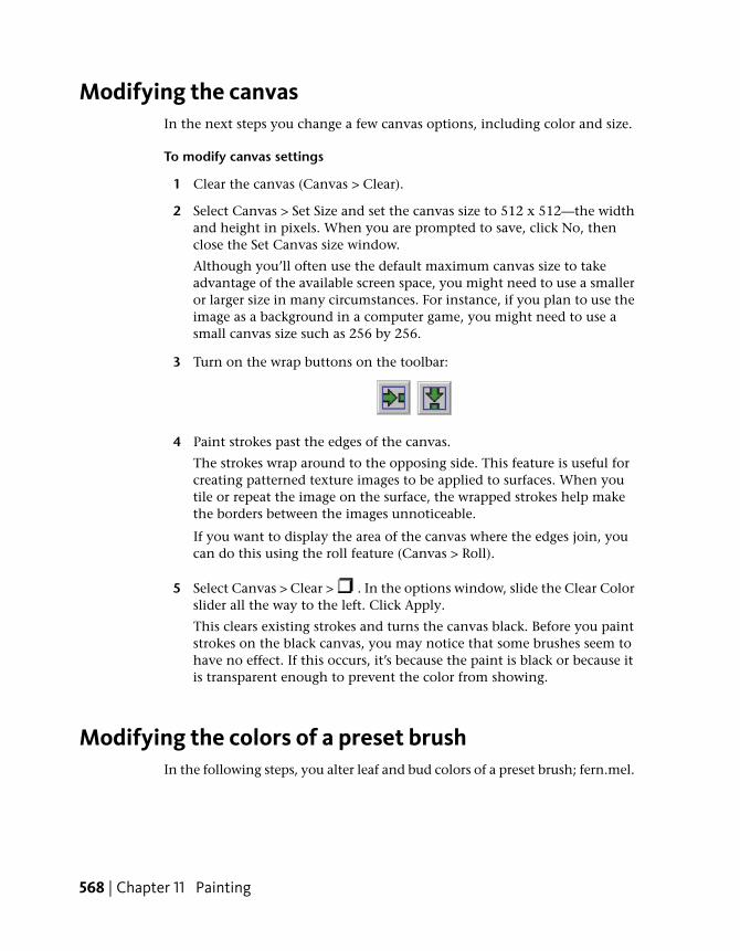
Modifying the canvasIn the next steps you change a few canvas options, including color and size.
To modify canvas settings
1 Clear the canvas (Canvas > Clear).
2 Select Canvas > Set Size and set the canvas size to 512 x 512—the widthand height in pixels. When you are prompted to save, click No, thenclose the Set Canvas size window.
Although you’ll often use the default maximum canvas size to takeadvantage of the available screen space, you might need to use a smalleror larger size in many circumstances. For instance, if you plan to use theimage as a background in a computer game, you might need to use asmall canvas size such as 256 by 256.
3 Turn on the wrap buttons on the toolbar:
4 Paint strokes past the edges of the canvas.
The strokes wrap around to the opposing side. This feature is useful forcreating patterned texture images to be applied to surfaces. When youtile or repeat the image on the surface, the wrapped strokes help makethe borders between the images unnoticeable.
If you want to display the area of the canvas where the edges join, youcan do this using the roll feature (Canvas > Roll).
5 Select Canvas > Clear > . In the options window, slide the Clear Colorslider all the way to the left. Click Apply.
This clears existing strokes and turns the canvas black. Before you paintstrokes on the black canvas, you may notice that some brushes seem tohave no effect. If this occurs, it’s because the paint is black or because itis transparent enough to prevent the color from showing.
Modifying the colors of a preset brushIn the following steps, you alter leaf and bud colors of a preset brush; fern.mel.
568 | Chapter 11 Painting

TIP When using the fern.mel brush, if any of the sliders do not appear, or appearcut off on the right, you need to increase the screen display resolution setting onyour monitor to 1280 X 1024.
To change the color of a brush
1 In the Visor (Brush > Get Brush), click the fern.mel preset brush in theplants folder.
2 Paint on the canvas to see the default display.
Because fern.mel uses tubes, ferns grow along the path of your stroke.
3 Resize the brush to a Global Scale of about 0.5 (Brush > Edit TemplateBrush) and paint on the canvas.
4 On the toolbar, click the L1 color box (Leaf Color 1), select a shade ofblue from the Color Chooser, and leave the Color Chooser open.
L1 sets the color of the tips of the leaves.
5 Click the L2 color box (Leaf Color 2) and select a shade of red from theColor Chooser.
L2 sets the color of the base of the leaves.
6 Click the B color box (Bud Color) and select a shade of yellow from theColor Chooser. B sets the color of the flower buds.
7 Paint on the canvas and observe how the changes you’ve made to thesettings affect the final paint effect.
TIP You can change the path width of fern.mel without changing the widthof the leaves and stems. Select Brush > Edit Template Brush to display theBrush Settings window, then in the Brush Profile section, change the valueof Brush Width. Similarly, you can alter the path width for any other presetstrokes with tubes.
Modifying the colors of a preset brush | 569
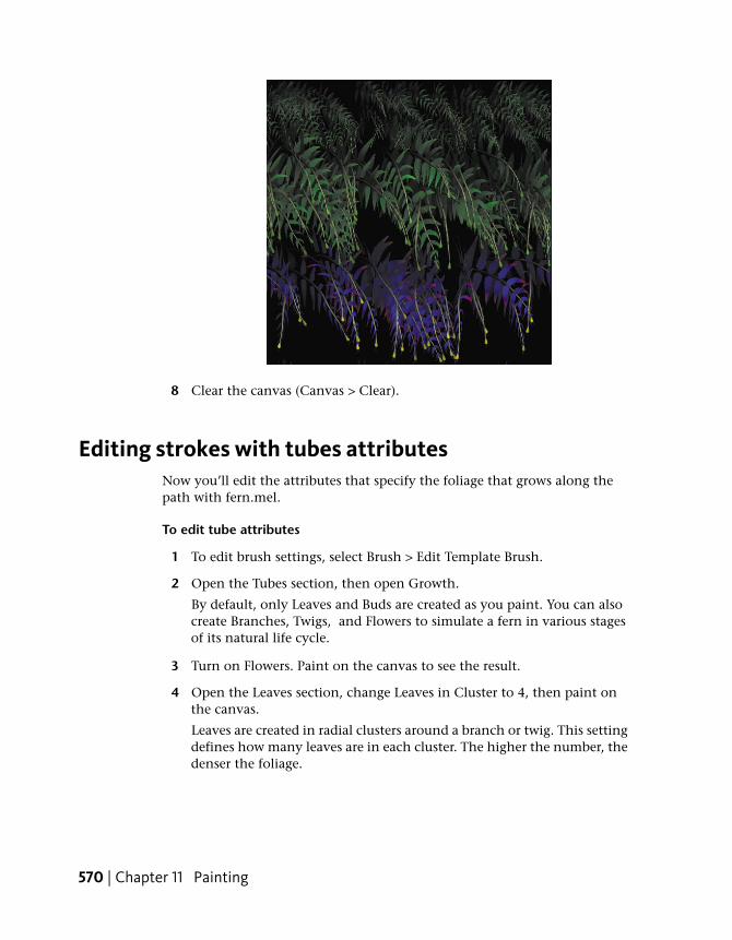
8 Clear the canvas (Canvas > Clear).
Editing strokes with tubes attributesNow you’ll edit the attributes that specify the foliage that grows along thepath with fern.mel.
To edit tube attributes
1 To edit brush settings, select Brush > Edit Template Brush.
2 Open the Tubes section, then open Growth.
By default, only Leaves and Buds are created as you paint. You can alsocreate Branches, Twigs, and Flowers to simulate a fern in various stagesof its natural life cycle.
3 Turn on Flowers. Paint on the canvas to see the result.
4 Open the Leaves section, change Leaves in Cluster to 4, then paint onthe canvas.
Leaves are created in radial clusters around a branch or twig. This settingdefines how many leaves are in each cluster. The higher the number, thedenser the foliage.
570 | Chapter 11 Painting

5 To make the flowers point in a different direction, open the Behaviorsection and then the Forces section. Set Path Follow to 0.1.
6 Paint to see the result.
Saving brush settings for future useWhen you first selected the preset brush fern.mel previously, Maya copied itto the template brush. You then edited the color and various other attributesof the template brush to create a unique ferns brush. The next steps show howto save the current settings of the template brush for future use.
To save a brush to the Shelf
1 On the main menu bar, select Paint Effects > Save Brush Preset. This isthe menu item you use to save the template brush as a preset brush.
2 Type the name blueFern in the Label box as well as the Overlay Labelbox.
This name appears in icons on the Shelf or Visor after you save the brush.
3 For the Save Preset option, turn on To Shelf. This means you’ll put thebrush on the Shelf but not in the Visor.
Saving brush settings for future use | 571

4 Click Grab Icon and drag a selection box around a part of the image thatis representative of the brush’s result.
A swatch appears in the window for the selected region. Repeat this stepuntil you are satisfied with the icon.
5 Click Save Brush Preset. An icon for the new preset brush appears on theShelf.
6 To check that the blueFern brush works, select a different preset brushand paint on the canvas, then select the blueFern from the Shelf andpaint on the canvas.
7 Clear the canvas and close the Save Brush Preset window.
Blending brushesYou can blend brushes. Before beginning, display the Visor, click gold.mel inthe metal folder, and paint on the canvas so you know gold’s effect. Do thesame for grassOrnament.mel from the grasses folder.
To blend brushes
1 Click grassOrnament.mel in the grasses folder.
2 From the menu, select Paint Effects > Preset Blending > .
The Preset Blending options window appears.
The brush preset blending is toggled on and the options in this windowset how much the template brush is influenced by the next preset brushyou select. This affects only the subsequent painting, not the presetbrushes in the Visor.
3 Change the Shading value to 80 and the Shape value to 0.
When you select the next brush (gold.mel), Maya uses 80% of its shadingand 0% of its shape. Conversely, the stroke uses 20% of thegrassOrnament.mel brush’s shading and 100% of its shape.
4 To confirm the effect, select gold.mel (in the metal folder), then painton the canvas.
5 Repeat the preceding steps, experimenting with different preset brushes,Shading, and Shape values. As a first try, blend flameCoarse.mel fromthe fire folder with the existing template brush. Set Shading to 60 andShape to 30.
572 | Chapter 11 Painting

If the Brush Preset Blend window is open, each time you select a presetbrush, its Shading and Shape values will be blended with the templatebrush.
6 Close the Brush Preset Blend window when you are done blendingbrushes.
7 Do not clear the canvas. You’ll use your existing strokes in the next steps.
Smearing, blurring, and erasing paintNow you’ll work with brush types that smear, blur, and erase paint.
To smear, blur, and erase paint
1 Select Brush > Reset Template Brush to select the default brush.
2 On the Brush menu, try the Smear, Blur, and Erase menu items and painton the strokes already on the canvas. You can also change these settingsusing the Brush Type setting in the Paint Effects Brush Settings window(Brush > Edit Template Brush).
3 If you need to perform compositing work, you can view the image’s alpha
channel by clicking this button: .
Smearing, blurring, and erasing paint | 573

White regions represent full opacity. Black represents full transparency.
4 If you turned on the alpha channel (Display > Alpha Channel), returnto the display of full color by selecting Display > All Channels.
5 Clear the canvas and restore the canvas color to white (Canvas > Clear >
).
6 To quit the canvas display and return to a scene view, select Panels >Perspective > persp (Hotkey 8).
7 In the Toolbox, click the Select Tool.
Clicking the Select Tool quits the Paint Effects Tool, and the mouse cursordisplays as an arrow.
8 Select Paint Effects > Preset Blending to turn off Preset Blending beforeyou proceed to the next lesson.
Beyond the lessonIn this lesson, you learned how to:
■ Use Paint Effects to paint on the 2D canvas.
■ Use the preset Paint Effects brushes from the Visor.
574 | Chapter 11 Painting

■ Edit, blend, and save preset brushes for later use.Painting on the 2D canvas is useful when you need to create a texture tobe applied to a surface. For example, suppose you paint a repeating brickpattern on the canvas and save the canvas as an image file. You can createa material, for instance, a Blinn material, then apply the image file as afile texture to the color of the Blinn material. You can then apply the Blinnmaterial to a 3D wall you’ve modeled, which creates the illusion of a brickwall.
Painting a 2D canvas is also useful for creating a background image for a scene.For instance, you might create lush foliage on the canvas, put it on a camera’simage plane, then use it as the backdrop for animated jungle animals in theforeground.
Although not covered in this lesson, you can use a tablet and stylus to paintwith pressure sensitivity. Pressure sensitivity allows you to more realisticallysimulate the effects of traditional drawing media (pens, pencils, markers, etc.)
Lesson 2: Painting in 3D using Paint Effects
Introduction
The Paint Effects Tool goes beyond traditional paint software by allowing youto paint directly in 3D space, either on the ground plane or on an object’ssurface. When you use Paint Effects for 3D work, the paint strokes arethree-dimensional and editable.
With Paint Effects, all of the hundreds of preset brushes found in the Visorunder the Paint Effects tab (airbrushes, pens, markers, watercolors, plants, fire,
Lesson 2: Painting in 3D using Paint Effects | 575
metal, flowers, trees, and underwater etc.) can be used to create 3D objects inyour scene. For example, you can use the preset plant brushes to paint a 3Dtropical fern garden around a walking character in your scene.
You can animate brush strokes to create dynamic effects. For example, youcan animate the ferns to shake in the wind or have them move when acharacter walks near them.
An electronic tablet with stylus is an ideal tool for painting with Paint Effects.With a real paint brush, pressing harder makes the brush wider and appliesthe paint more thickly. You can achieve the same effect with Paint Effects byspecifying the effect of pressure on the stylus for each stroke and the thresholdof response to pressure. You can map up to three attribute values to styluspressure and edit them as you work.
When you use Paint Effects to paint 3D strokes, you can edit the brush andstroke attributes to create a variety of effects.
In this lesson, you begin to explore what is possible with painting in 3D usingthe Paint Effects Tool by learning how to:
■ Paint directly in the 3D scene view.
■ Choose brushes from the Visor and the Shelf and modify their brushattributes.
■ Paint in 3D using the Paint Effects panel.
■ Differentiate between paint brushes and paint strokes.
■ Make surfaces paintable so paint strokes can be applied to them.
■ Select brush strokes and modify their attributes.
■ View strokes in wireframe and rendered mode.
■ Apply various effects to stroke attributes.
Preparing for the lessonsTo ensure the lessons work as described, do these steps before beginning:
1 If you have not done so already, consider doing the lessons in theRendering section of this guide. Familiarity with Maya rendering conceptsis important to understanding the lessons.
2 Select File > New Scene to create a new scene.
576 | Chapter 11 Painting

If you just finished Lesson 1 in this chapter you may be presented witha window asking if you wish to Save previous paint effects. Select No.
3 To use all available screen space, maximize the Maya window.
4 From a panel menu bar, select Panels > Layouts > Single Pane.
5 Select the Rendering menu set. Unless otherwise noted, the directions inthis chapter assume the Rendering menu set is selected.
6 From the Shelf, select the Paint Effects tab to display the various presetbrushes.
If the Paint Effects Shelf tab does not appear as part of the shelf set, seethe Maya Help for Shelves. (For Linux users, any new shelves do not loadby default.)
Regardless of your operating system, the Paint Effects preset brushes areaccessible from the Visor panel. (From a view panel, select Panels > Panel> Visor.)
Brushes and strokesLike a traditional paint program, Paint Effects allows you to use a brush andpaint strokes. In Paint Effects, the brush and stroke have unique qualities andcharacteristics.
A brush contains the various attributes that define the appearance and behaviorof the paint. The template brush settings define the initial settings for a brush.
When you drag the Paint Effects brush, you create a path for the brush calledthe paint stroke.
A stroke is a 3D curve (or collection of curves) with attributes that define howthe paint is applied along the stroke path. You can paint strokes directly inthe 3D scene or on objects.
When you select a brush preset from the shelf or from the Visor, that brushis copied to the template brush. Any changes you make to the template brushsettings affect what the next stroke looks like, but they do not affect anypreviously painted strokes.
To select a Paint Effects preset brush from the Shelf
1 From the Toolbox panel layout shortcuts, select the Single PerspectiveView.
Brushes and strokes | 577
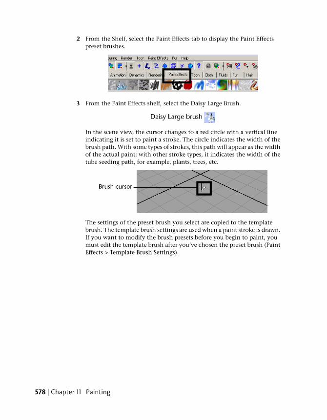
2 From the Shelf, select the Paint Effects tab to display the Paint Effectspreset brushes.
3 From the Paint Effects shelf, select the Daisy Large Brush.
In the scene view, the cursor changes to a red circle with a vertical lineindicating it is set to paint a stroke. The circle indicates the width of thebrush path. With some types of strokes, this path will appear as the widthof the actual paint; with other stroke types, it indicates the width of thetube seeding path, for example, plants, trees, etc.
The settings of the preset brush you select are copied to the templatebrush. The template brush settings are used when a paint stroke is drawn.If you want to modify the brush presets before you begin to paint, youmust edit the template brush after you’ve chosen the preset brush (PaintEffects > Template Brush Settings).
578 | Chapter 11 Painting
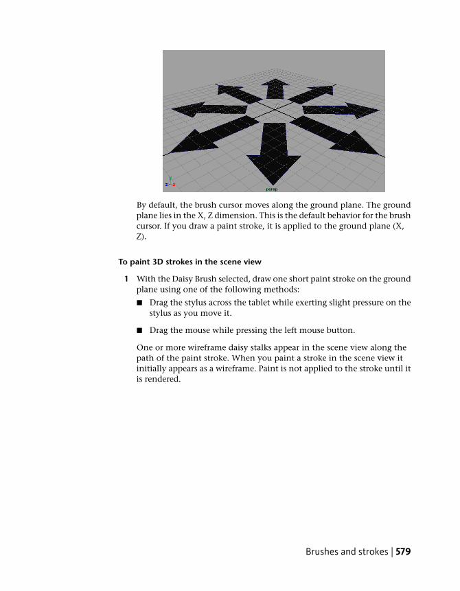
By default, the brush cursor moves along the ground plane. The groundplane lies in the X, Z dimension. This is the default behavior for the brushcursor. If you draw a paint stroke, it is applied to the ground plane (X,Z).
To paint 3D strokes in the scene view
1 With the Daisy Brush selected, draw one short paint stroke on the groundplane using one of the following methods:
■ Drag the stylus across the tablet while exerting slight pressure on thestylus as you move it.
■ Drag the mouse while pressing the left mouse button.
One or more wireframe daisy stalks appear in the scene view along thepath of the paint stroke. When you paint a stroke in the scene view itinitially appears as a wireframe. Paint is not applied to the stroke until itis rendered.
Brushes and strokes | 579

The stalks that extend out of the curve or stroke are called tubes. In PaintEffects, strokes are either simple strokes or strokes with tubes.
Because the stroke has a curve associated with it, you can move, scale, orrotate the stroke like other objects in the scene. You can edit the curveto modify the shape of the stroke path.
2 Dolly and tumble the scene to better view these strokes with tubes in 3D.
3 Select the Move Tool from the Toolbox.
A move manipulator icon appears at the X, Y, Z origin. (If the movemanipulator does not appear, you can click on the stroke to reselect itwith the Move Tool.)
4 In the scene view, drag any of the Move Tool manipulator arrows toreposition the stroke.
Each time you paint a stroke, Paint Effects creates a new brush and strokenode and attaches them to the stroke that is created. You can modify thesebrush and stroke nodes once they’ve been created. To edit these brush orstroke attributes, you use the Attribute Editor.
580 | Chapter 11 Painting
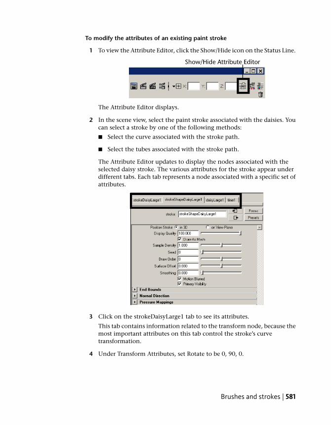
To modify the attributes of an existing paint stroke
1 To view the Attribute Editor, click the Show/Hide icon on the Status Line.
The Attribute Editor displays.
2 In the scene view, select the paint stroke associated with the daisies. Youcan select a stroke by one of the following methods:
■ Select the curve associated with the stroke path.
■ Select the tubes associated with the stroke path.
The Attribute Editor updates to display the nodes associated with theselected daisy stroke. The various attributes for the stroke appear underdifferent tabs. Each tab represents a node associated with a specific set ofattributes.
3 Click on the strokeDaisyLarge1 tab to see its attributes.
This tab contains information related to the transform node, because themost important attributes on this tab control the stroke’s curvetransformation.
4 Under Transform Attributes, set Rotate to be 0, 90, 0.
Brushes and strokes | 581
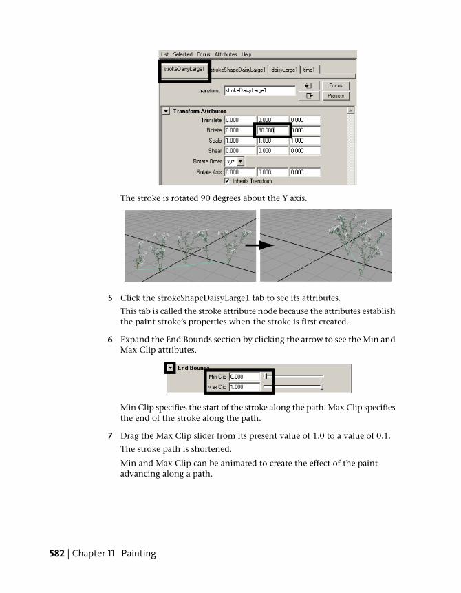
The stroke is rotated 90 degrees about the Y axis.
5 Click the strokeShapeDaisyLarge1 tab to see its attributes.
This tab is called the stroke attribute node because the attributes establishthe paint stroke’s properties when the stroke is first created.
6 Expand the End Bounds section by clicking the arrow to see the Min andMax Clip attributes.
Min Clip specifies the start of the stroke along the path. Max Clip specifiesthe end of the stroke along the path.
7 Drag the Max Clip slider from its present value of 1.0 to a value of 0.1.
The stroke path is shortened.
Min and Max Clip can be animated to create the effect of the paintadvancing along a path.
582 | Chapter 11 Painting

8 Drag the Max Clip slider back to its original value of 1.0.
9 Click the daisyLarge1 attribute tab to see its attributes.
This is the node that contains attributes related to the paint brushassociated with the stroke.
10 Set the Global Scale attribute to 6.0.
The daisies scale larger along the stroke’s path.
11 In the daisyLarge1 node, expand the Tubes attributes, then Behavior andForces.
Brushes and strokes | 583
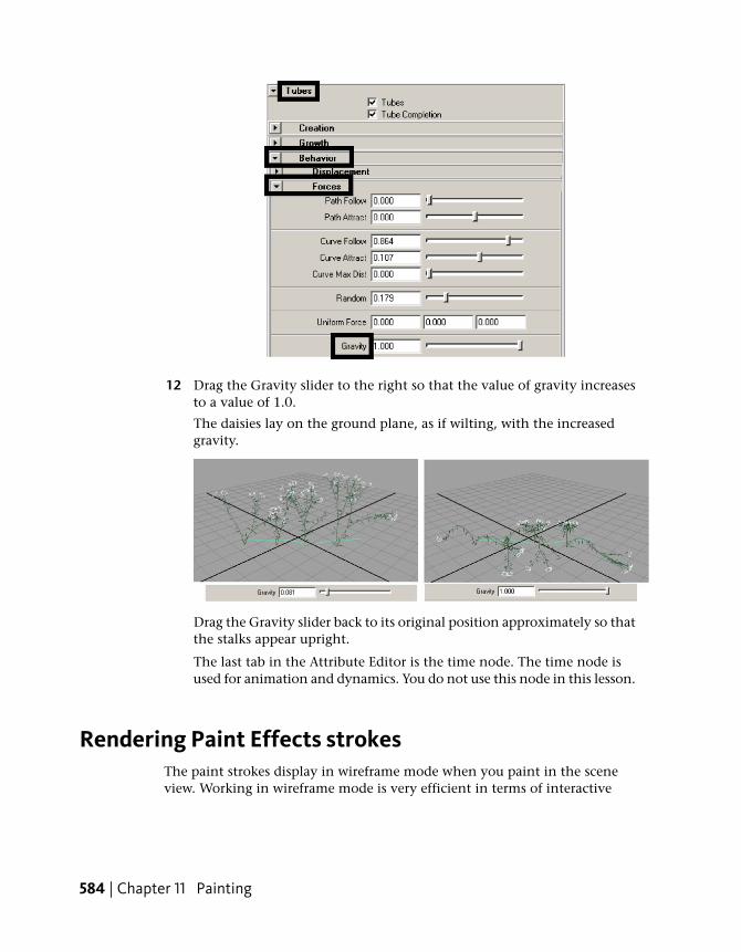
12 Drag the Gravity slider to the right so that the value of gravity increasesto a value of 1.0.
The daisies lay on the ground plane, as if wilting, with the increasedgravity.
Drag the Gravity slider back to its original position approximately so thatthe stalks appear upright.
The last tab in the Attribute Editor is the time node. The time node isused for animation and dynamics. You do not use this node in this lesson.
Rendering Paint Effects strokesThe paint strokes display in wireframe mode when you paint in the sceneview. Working in wireframe mode is very efficient in terms of interactive
584 | Chapter 11 Painting
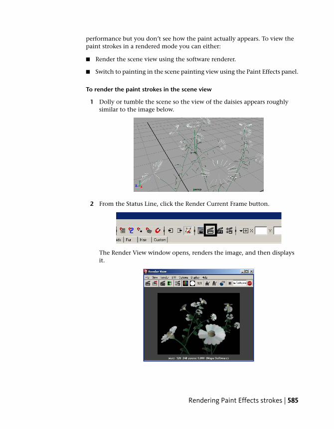
performance but you don’t see how the paint actually appears. To view thepaint strokes in a rendered mode you can either:
■ Render the scene view using the software renderer.
■ Switch to painting in the scene painting view using the Paint Effects panel.
To render the paint strokes in the scene view
1 Dolly or tumble the scene so the view of the daisies appears roughlysimilar to the image below.
2 From the Status Line, click the Render Current Frame button.
The Render View window opens, renders the image, and then displaysit.
Rendering Paint Effects strokes | 585
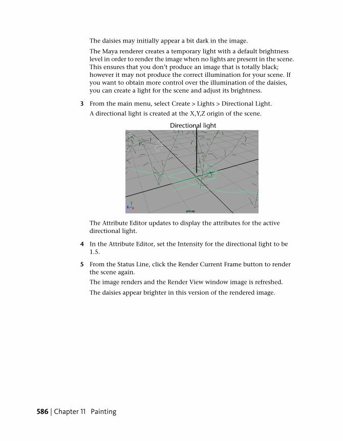
The daisies may initially appear a bit dark in the image.
The Maya renderer creates a temporary light with a default brightnesslevel in order to render the image when no lights are present in the scene.This ensures that you don’t produce an image that is totally black;however it may not produce the correct illumination for your scene. Ifyou want to obtain more control over the illumination of the daisies,you can create a light for the scene and adjust its brightness.
3 From the main menu, select Create > Lights > Directional Light.
A directional light is created at the X,Y,Z origin of the scene.
The Attribute Editor updates to display the attributes for the activedirectional light.
4 In the Attribute Editor, set the Intensity for the directional light to be1.5.
5 From the Status Line, click the Render Current Frame button to renderthe scene again.
The image renders and the Render View window image is refreshed.
The daisies appear brighter in this version of the rendered image.
586 | Chapter 11 Painting

6 Close the Render View window.
Sometimes you may want to view your painted strokes as you paint. To dothis, you can paint in the Paint Effects panel view and use the scene paintingview mode.
To display rendered paint strokes as you paint
1 Press 8 to switch to the Paint Effects panel.
NOTE If the 2D Paint Canvas appears instead (i.e.: panel appears white),select Paint > Paint Scene, from the panel menu.
The Paint Effects panel menu and toolbar displays as well as the scenepainting view. This panel allows you to paint in scene painting viewmode.
Rendering Paint Effects strokes | 587

The scene painting view is a snapshot of the modeling view. In this viewyou can both paint and view your strokes in a rendered fashion to seewhat they will really look like as you work.
You can dolly, track, and tumble in the scene painting view. You canselect objects by pressing the Ctrl key and clicking on them. If you wantto move, or otherwise manipulate 3D objects in the scene view, you mustexit the Paint Effects panel by pressing the 8 key again.
2 With the Daisy Brush selected, paint a stroke in the scene painting view.
The new stroke displays in rendered mode. If you dolly or track the scenepainting view, any rendered strokes will revert back to wireframe displayuntil you refresh the rendered display.
3 To automatically update the paint strokes so they display in renderedmode, select Stroke Refresh > Rendered.
It will take a few moments for the rendering of all of the paint strokes tobe calculated and then displayed.
Each time you adjust the camera view while working in scene paintingmode with Refresh > Rendered turned on, the system will automaticallyupdate the rendering based on the new view.
Automatically refreshing the rendering can be time-consuming dependingon the complexity of paint strokes in your scene. Alternatively, you canset the rendering to refresh only when you manually choose to do so.
4 From the Paint Effects panel menu, select Stroke Refresh > Off.
588 | Chapter 11 Painting

Now you must manually refresh the Paint Effects rendered view usingthe Redraw Paint Effects view button in order to see the paint strokesrendered.
5 Dolly the view to obtain a closer view of the daisies.
6 Manually refresh the rendering of the daisies by clicking the Redraw PaintEffects view button.
7 Exit the scene painting view mode by pressing the 8 key.
Paint Effects on 3D objects
With Paint Effects, you can paint 3D strokes directly on 3D objects in a Mayascene.
Paint Effects on 3D objects | 589

In this section, you create a surface for an underwater terrain and sculpt it tothe desired form using the Sculpt Geometry tool. You use the underwaterpreset Paint Effects brushes found in the Visor to begin the underwater scene.
Creating a surface to paint onIn Paint Effects, NURBS surfaces are the only surface type you can paint on.You will create a NURBS plane, and sculpt it to make its surface appear likean underwater terrain.
To create a surface terrain for the underwater scene
1 Select File > New Scene.
A new empty scene is created.
2 From the main menu, select Create > NURBS Primitives > Plane > .
The NURBS plane options window appears.
3 In the NURBS Plane Options window, select Edit > Reset settings andthen set the following options:
■ Width: 15
■ Length: 15
■ U Patches: 10
■ V Patches: 10
4 In the NURBS Plane Options window, click Create.
Maya creates a plane primitive and positions it at the origin. The planeis 15 units by 15 units in dimension with 10 subdivisions along each side.
590 | Chapter 11 Painting
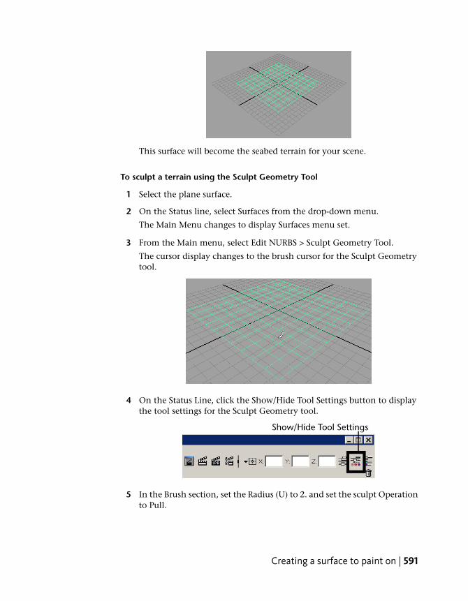
This surface will become the seabed terrain for your scene.
To sculpt a terrain using the Sculpt Geometry Tool
1 Select the plane surface.
2 On the Status line, select Surfaces from the drop-down menu.
The Main Menu changes to display Surfaces menu set.
3 From the Main menu, select Edit NURBS > Sculpt Geometry Tool.
The cursor display changes to the brush cursor for the Sculpt Geometrytool.
4 On the Status Line, click the Show/Hide Tool Settings button to displaythe tool settings for the Sculpt Geometry tool.
5 In the Brush section, set the Radius (U) to 2. and set the sculpt Operationto Pull.
Creating a surface to paint on | 591

6 Drag the cursor along the back right edge of the plane to pull it upwardsas shown.
7 Drag the cursor along the back left edge of the plane to pull it upwards.
8 Dolly and track the view as required so you can easily view the areas youneed to sculpt.
9 Sculpt along the front and middle of the plane to make some bumpyareas.
10 Repeat steps 7 through 10 until you have your 3D terrain looking roughlyas shown in the image below.
TIP If you want to undo a particular sculpt operation, click Ctrl + z to undothe sculpt stroke. You can click Ctrl + z repeatedly to undo a number of sculptoperations.
592 | Chapter 11 Painting
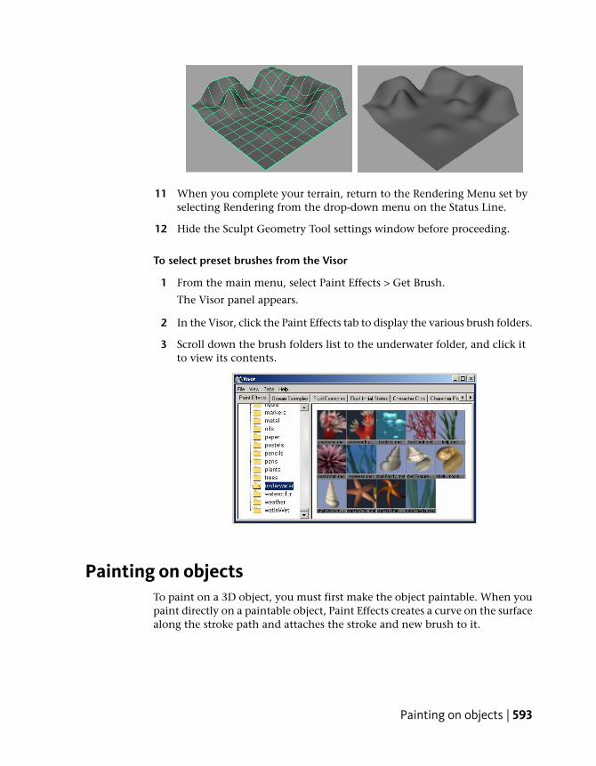
11 When you complete your terrain, return to the Rendering Menu set byselecting Rendering from the drop-down menu on the Status Line.
12 Hide the Sculpt Geometry Tool settings window before proceeding.
To select preset brushes from the Visor
1 From the main menu, select Paint Effects > Get Brush.
The Visor panel appears.
2 In the Visor, click the Paint Effects tab to display the various brush folders.
3 Scroll down the brush folders list to the underwater folder, and click itto view its contents.
Painting on objectsTo paint on a 3D object, you must first make the object paintable. When youpaint directly on a paintable object, Paint Effects creates a curve on the surfacealong the stroke path and attaches the stroke and new brush to it.
Painting on objects | 593

If you make an object paintable and then try to paint on one that is notpaintable, no stroke occurs. If you don’t make any objects in your scenepaintable, your strokes are placed on the ground plane.
To paint on a 3D object
1 With the terrain surface selected, select Paint Effects > Make Paintable.
2 From the Visor, select the brush named kelp.mel.
3 Paint a short stroke onto your 3D terrain surface.
When you paint directly on a paintable object, Paint Effects creates acurve on the surface along the stroke path and attaches the stroke andnew brush to it. If you move the plane, the paint stroke moves with it.
4 Paint a few more kelp strands throughout the scene as shown.
The kelp brush orients the tubes to point along the normal of the surfaceyou paint on. In the ocean, kelp grows towards the surface of the waterin a vertical manner. If you want your kelp to appear realistic, it shouldpoint vertically upwards. If you paint the kelp on an angled part of thesurface, the kelp tube will not point in a vertical direction.
TIP If you want to change the scale of the Paint Effects stroke to obtain largerplants or animals, press the b key and drag your stylus or mouse to the leftor right to make the global scale for the current brush smaller or larger.
If you want to change the width of the brush stroke, to paint a narrower orwider tube path, for example, a wider swath of kelp plants, press the shiftand b key and drag to the left or right.
594 | Chapter 11 Painting
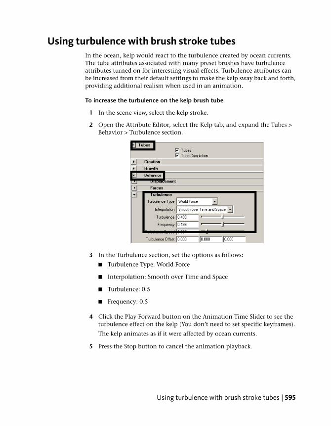
Using turbulence with brush stroke tubesIn the ocean, kelp would react to the turbulence created by ocean currents.The tube attributes associated with many preset brushes have turbulenceattributes turned on for interesting visual effects. Turbulence attributes canbe increased from their default settings to make the kelp sway back and forth,providing additional realism when used in an animation.
To increase the turbulence on the kelp brush tube
1 In the scene view, select the kelp stroke.
2 Open the Attribute Editor, select the Kelp tab, and expand the Tubes >Behavior > Turbulence section.
3 In the Turbulence section, set the options as follows:
■ Turbulence Type: World Force
■ Interpolation: Smooth over Time and Space
■ Turbulence: 0.5
■ Frequency: 0.5
4 Click the Play Forward button on the Animation Time Slider to see theturbulence effect on the kelp (You don’t need to set specific keyframes).
The kelp animates as if it were affected by ocean currents.
5 Press the Stop button to cancel the animation playback.
Using turbulence with brush stroke tubes | 595

You can adjust the turbulence settings while viewing the playback. If theframe range is too short, you can modify it to suit your needs.
Using additional preset brushes1 From the Visor, select the brush named fanCoral.mel.
2 Paint a few fan coral strokes in your scene near the back edges of theplane.
TIP If you paint a stroke in your scene and want to delete it you can do soby one of the following methods:
■ Press Ctrl + z to immediately undo the stroke.
■ Click on the stroke to select it and then press the Delete key.
■ Marquee-select a tube associated with the stroke and then press theDelete key.
■ Marquee-select multiple tubes and strokes and then press the Deletekey.
If you want to delete all the paint strokes in your scene you can select Edit >Delete All by Type.
3 Paint additional strokes in your underwater scene using a few using thefollowing brushes found in the underwater folder in the Visor:
■ sea urchins, starfish, seashells, and anemones
4 Dolly and track the scene for a closer view so it appears approximatelyas shown.
596 | Chapter 11 Painting

5 From the Status Line, click the Render Current Frame button.
6 The renderer executes, renders the image, and then displays it in theRender View window.
You can create a seabed texture for the plane primitive, a few rocks, and someanimated fish swimming to complete your scene.
You can spend additional time to further refine this scene, but this examplegives you an idea of how a scene with various 3D props can be quicklyestablished using Paint Effects and the various preset brushes found in theVisor.
Using additional preset brushes | 597

Mesh brushes
Mesh brushes are a brush type that provide special features not available withother Paint Effect brush types. Mesh brushes render using polygonal trianglesrather than brush stamps. As a result, mesh strokes can be more accuratelytexture-mapped for realistic results. They also appear more realistic comparedto other brush types whether they are viewed close-up or from a distance.
The mesh brush stroke can also be converted to a polygonal surface in theMaya scene. Once the stroke is converted to polygons, the resulting polygonscan be modified using any of the Maya polygonal modification tools andutilized like any other polygonal surface (animation, rendering, and so on)
In this section, you are introduced to mesh brushes and learn additionaltechniques related to the various brush and stroke attributes. You learn howto:
■ Understand the structure of strokes with tubes.
■ Modify a variety brush tube attributes.
■ Convert the mesh brush stroke to polygons.
■ Modify the converted mesh using construction history.
■ Render the polygonal meshes.
To select a mesh brush preset from the Shelf
1 Select File > New Scene.
A new empty scene is created.
2 From the Toolbox panel layout shortcuts, select the Single PerspectiveView.
598 | Chapter 11 Painting

3 From the Shelf, select the Paint Effects tab to display the Paint Effectspreset brushes.
4 From the Paint Effects shelf, select the Teapot Brush.
In the scene view, the cursor changes to a sphere icon indicating it is setto paint a stroke. The Teapot Brush is a mesh brush type.
5 In the scene view, drag your mouse or stylus along the ground plane tocreate one short stroke.
6 Dolly and tumble the view to see the wireframe version of the stroke.
The teapot stroke displays three wireframe tubes to represent the teapot.These tubes represent the body, spout, and handle for the teapot.
Paint Effects uses a plant or tree archetype to represent the various tubeattributes. If you envision how a plant or tree has a trunk, out from whichbranches, leaves, flowers, and buds grow, you understand how eachattribute is controlled in the attribute editor.
The center vertical line represents the main tube, whose attributes arefound in the Creation tab of the attribute editor. The diagonal andsemicircular lines represent the Leaves and Flowers tube attributes for thespout and handle of the teapot.
Mesh brushes | 599

To render the paint effects stroke
1 From the Status Line, click the Render Current Frame button.
The renderer executes, renders the paint stroke, and then displays theimage in a Render View window.
2 Close the Render View window.
Mesh brush types are useful for representing hard surfaces compared to otherbrush types (the teapot is one example).
Converting mesh strokes to polygonsMesh strokes can be converted to polygons. Converting the mesh stroke topolygons allows you to visualize any brush modifications you make in theAttribute Editor without having to render the stroke. It is possible to edit,animate, and render the converted polygon mesh the same way you wouldany other polygonal surface types.
To convert a mesh stroke to polygons
1 Press the q key (Hotkey) to choose the Select Tool.
The cursor changes to an arrow icon indicating the change to selectionmode.
600 | Chapter 11 Painting
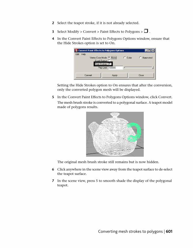
2 Select the teapot stroke, if it is not already selected.
3 Select Modify > Convert > Paint Effects to Polygons > .
4 In the Convert Paint Effects to Polygons Options window, ensure thatthe Hide Strokes option is set to On.
Setting the Hide Strokes option to On ensures that after the conversion,only the converted polygon mesh will be displayed.
5 In the Convert Paint Effects to Polygons Options window, click Convert.
The mesh brush stroke is converted to a polygonal surface. A teapot modelmade of polygons results.
The original mesh brush stroke still remains but is now hidden.
6 Click anywhere in the scene view away from the teapot surface to de-selectthe teapot surface.
7 In the scene view, press 5 to smooth shade the display of the polygonalteapot.
Converting mesh strokes to polygons | 601
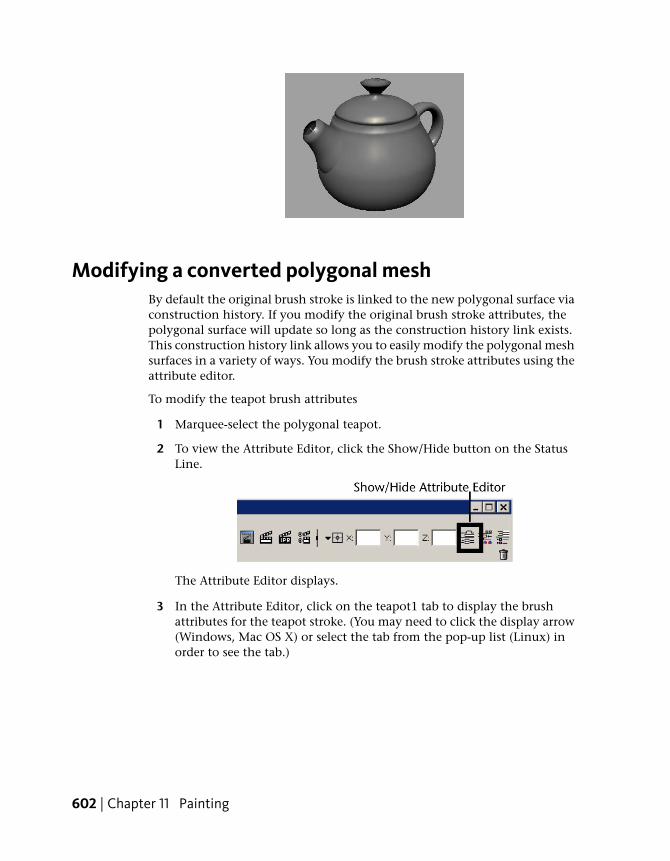
Modifying a converted polygonal meshBy default the original brush stroke is linked to the new polygonal surface viaconstruction history. If you modify the original brush stroke attributes, thepolygonal surface will update so long as the construction history link exists.This construction history link allows you to easily modify the polygonal meshsurfaces in a variety of ways. You modify the brush stroke attributes using theattribute editor.
To modify the teapot brush attributes
1 Marquee-select the polygonal teapot.
2 To view the Attribute Editor, click the Show/Hide button on the StatusLine.
The Attribute Editor displays.
3 In the Attribute Editor, click on the teapot1 tab to display the brushattributes for the teapot stroke. (You may need to click the display arrow(Windows, Mac OS X) or select the tab from the pop-up list (Linux) inorder to see the tab.)
602 | Chapter 11 Painting

4 In the Attribute Editor, expand the Mesh attributes section to display itsattributes.
5 In the Mesh attributes, drag the Tubes Sections slider to the left to a valueof 3.
The body, spout, and handle of the teapot update to display as 3 sidedsurfaces.
Modifying a converted polygonal mesh | 603
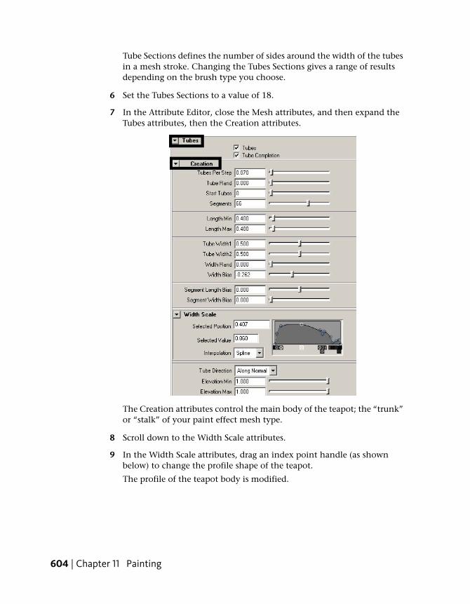
Tube Sections defines the number of sides around the width of the tubesin a mesh stroke. Changing the Tubes Sections gives a range of resultsdepending on the brush type you choose.
6 Set the Tubes Sections to a value of 18.
7 In the Attribute Editor, close the Mesh attributes, and then expand theTubes attributes, then the Creation attributes.
The Creation attributes control the main body of the teapot; the “trunk”or “stalk” of your paint effect mesh type.
8 Scroll down to the Width Scale attributes.
9 In the Width Scale attributes, drag an index point handle (as shownbelow) to change the profile shape of the teapot.
The profile of the teapot body is modified.
604 | Chapter 11 Painting
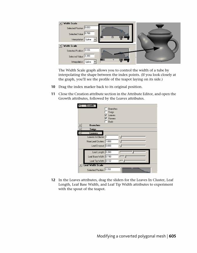
The Width Scale graph allows you to control the width of a tube byinterpolating the shape between the index points. (If you look closely atthe graph, you’ll see the profile of the teapot laying on its side.)
10 Drag the index marker back to its original position.
11 Close the Creation attribute section in the Attribute Editor, and open theGrowth attributes, followed by the Leaves attributes.
12 In the Leaves attributes, drag the sliders for the Leaves In Cluster, LeafLength, Leaf Base Width, and Leaf Tip Width attributes to experimentwith the spout of the teapot.
Modifying a converted polygonal mesh | 605
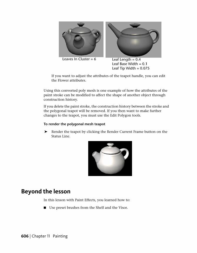
If you want to adjust the attributes of the teapot handle, you can editthe Flower attributes.
Using this converted poly mesh is one example of how the attributes of thepaint stroke can be modified to affect the shape of another object throughconstruction history.
If you delete the paint stroke, the construction history between the stroke andthe polygonal teapot will be removed. If you then want to make furtherchanges to the teapot, you must use the Edit Polygon tools.
To render the polygonal mesh teapot
➤ Render the teapot by clicking the Render Current Frame button on theStatus Line.
Beyond the lessonIn this lesson with Paint Effects, you learned how to:
■ Use preset brushes from the Shelf and the Visor.
606 | Chapter 11 Painting
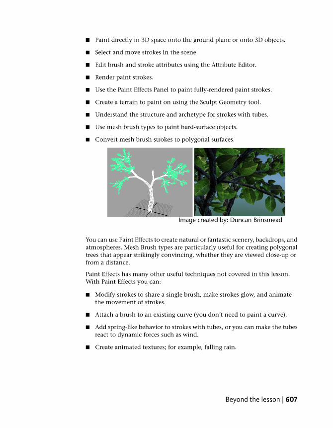
■ Paint directly in 3D space onto the ground plane or onto 3D objects.
■ Select and move strokes in the scene.
■ Edit brush and stroke attributes using the Attribute Editor.
■ Render paint strokes.
■ Use the Paint Effects Panel to paint fully-rendered paint strokes.
■ Create a terrain to paint on using the Sculpt Geometry tool.
■ Understand the structure and archetype for strokes with tubes.
■ Use mesh brush types to paint hard-surface objects.
■ Convert mesh brush strokes to polygonal surfaces.
You can use Paint Effects to create natural or fantastic scenery, backdrops, andatmospheres. Mesh Brush types are particularly useful for creating polygonaltrees that appear strikingly convincing, whether they are viewed close-up orfrom a distance.
Paint Effects has many other useful techniques not covered in this lesson.With Paint Effects you can:
■ Modify strokes to share a single brush, make strokes glow, and animatethe movement of strokes.
■ Attach a brush to an existing curve (you don’t need to paint a curve).
■ Add spring-like behavior to strokes with tubes, or you can make the tubesreact to dynamic forces such as wind.
■ Create animated textures; for example, falling rain.
Beyond the lesson | 607

■ Paint using a Thin Line brush type which allows you to render largenumbers of fine tubes much more quickly than the Paint Brush type. Thisbrush type is useful for painting hair.
Lesson 3: Painting textures on surfaces
IntroductionThe 3D Paint Tool allows you to paint textures directly onto a model’s surface.In this lesson, you paint colors, patterns, and textures on a dinosaur model.In this lesson you learn how to:
■ Prepare a surface model for painting.
■ Paint on a surface using both Artisan and Paint Effects brushes.
■ Use reflected paint strokes for symmetrical effects.
■ Flood fill an entire 3D model with paint.
■ Modify brush shapes and stamp settings.
■ Paint a bump map texture directly on a surface.
Open the scene for the lessonYou will paint a dinosaur model we prepared for this lesson.
1 Do the steps outlined in Preparing for the lessons on page 562.
2 Open the scene file named 3DPaint.mb.
This file can be found in the GettingStarted directory that you set asyour Maya project:
GettingStarted/Paint/3DPaint.mb
608 | Chapter 11 Painting
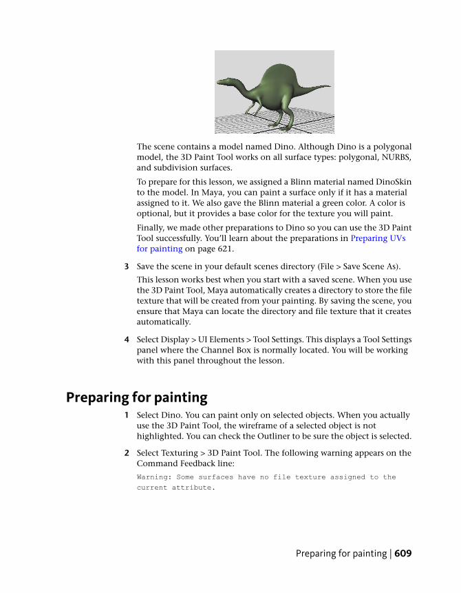
The scene contains a model named Dino. Although Dino is a polygonalmodel, the 3D Paint Tool works on all surface types: polygonal, NURBS,and subdivision surfaces.
To prepare for this lesson, we assigned a Blinn material named DinoSkinto the model. In Maya, you can paint a surface only if it has a materialassigned to it. We also gave the Blinn material a green color. A color isoptional, but it provides a base color for the texture you will paint.
Finally, we made other preparations to Dino so you can use the 3D PaintTool successfully. You’ll learn about the preparations in Preparing UVsfor painting on page 621.
3 Save the scene in your default scenes directory (File > Save Scene As).
This lesson works best when you start with a saved scene. When you usethe 3D Paint Tool, Maya automatically creates a directory to store the filetexture that will be created from your painting. By saving the scene, youensure that Maya can locate the directory and file texture that it createsautomatically.
4 Select Display > UI Elements > Tool Settings. This displays a Tool Settingspanel where the Channel Box is normally located. You will be workingwith this panel throughout the lesson.
Preparing for painting1 Select Dino. You can paint only on selected objects. When you actually
use the 3D Paint Tool, the wireframe of a selected object is nothighlighted. You can check the Outliner to be sure the object is selected.
2 Select Texturing > 3D Paint Tool. The following warning appears on theCommand Feedback line:
Warning: Some surfaces have no file texture assigned to the
current attribute.
Preparing for painting | 609

The 3D Paint Tool requires that the material assigned to your model hasa file texture applied to it. Because there is no file texture yet assigned,the warning appears.
When you move the cursor over Dino, you see a circle-X icon thatindicates you cannot paint on the model.
3 To make sure you have the default settings for the 3D Paint Tool, clickReset Tool at the top of the 3D Paint Tool settings panel.
4 In the File Textures section of the 3D Paint Tool settings panel, set theAttribute to Paint setting to Color, then click Assign/Edit Textures.
This step and the next two steps assign a texture to Dino. (Note that youcan also paint over an existing texture that you assigned fromHypershade.)
5 Type 512 in the Size X box, which is the height of the new file texture inpixels.
By increasing the file texture size, you will see finer detail and resolutionin a rendered image of your painting. The number 512 is twice the defaultsize, 256. You could use a higher resolution, but sizes larger than 512slow the interactive speed as you paint. Notice that Size Y automaticallychanges to 512. This is because Keep Aspect Ratio is turned on, ensuringthat the proportions of the texture are maintained.
6 Click Assign/Edit Textures in the Assign/Edit File Textures window.
Maya creates a file texture and assigns it to the Color attribute of theDinoSkin material. At the end of the lesson you will learn about the nameand location of the file texture that is created.
You are now ready to paint.
610 | Chapter 11 Painting
Painting with an Artisan brushIn the following steps, you paint various colors on the texture you justassigned. You also change the size of the brush strokes.
There are two types of brushes you can use. The default is the Artisan brush,which you’ll use in the next steps. (Artisan refers to a group of painting toolsin Maya that share common tool settings.) The other brush is based on thePaint Effects brushes; you’ll use it later in the lesson.
To paint using an Artisan brush
1 If you have a tablet and pen, you can experiment with pressure sensitivityas you paint. Open the Stylus Pressure section and turn on Stylus Pressure.(You do not need to have a tablet and pen to complete the lesson.)
By default, when you paint with Artisan brushes, the pressure you applyto the pen affects the Opacity setting of the 3D Paint Tool. The harderyou press, the more opaque the stroke.
2 In the Color section of the Tool Settings, click the box next to Color andselect a color in the Color Chooser. Leave the Color Chooser open. You’lluse it in the next few steps.
3 Paint a stroke by dragging on the model.
4 Select another color from the Color Chooser and paint over your firststroke.
The new color paints over the first color by default. Note that you canblend the colors by choosing a different Blend Mode setting, under thePaint Operations heading. You won’t blend the colors in this lesson.
5 Move the brush onto Dino, hold down the b key and drag to the left tomake the brush smaller. Drag until the number at the brush icon changesto about 0.5. You don’t need to be precise.
Use this hotkey when you need to change the brush width. To make thebrush wider, drag to the right. You can also change the width by changingthe Radius (U) setting.
Painting with an Artisan brush | 611
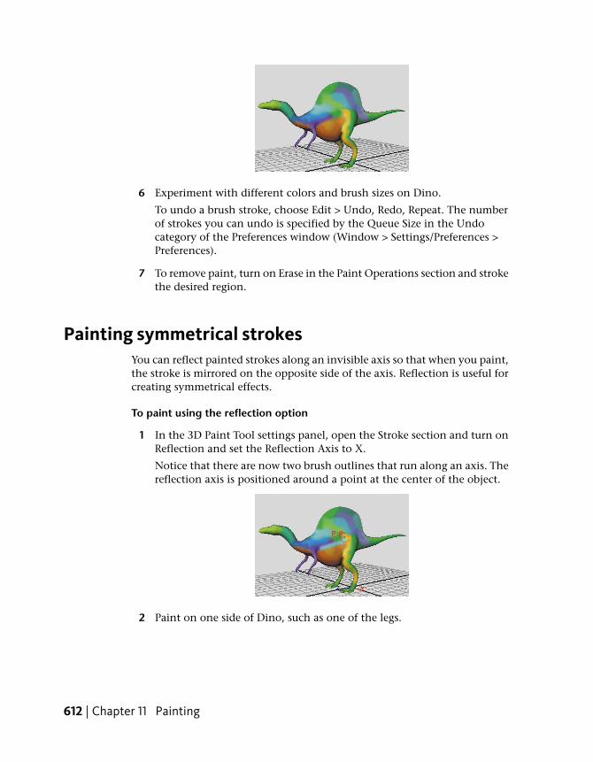
6 Experiment with different colors and brush sizes on Dino.
To undo a brush stroke, choose Edit > Undo, Redo, Repeat. The numberof strokes you can undo is specified by the Queue Size in the Undocategory of the Preferences window (Window > Settings/Preferences >Preferences).
7 To remove paint, turn on Erase in the Paint Operations section and strokethe desired region.
Painting symmetrical strokesYou can reflect painted strokes along an invisible axis so that when you paint,the stroke is mirrored on the opposite side of the axis. Reflection is useful forcreating symmetrical effects.
To paint using the reflection option
1 In the 3D Paint Tool settings panel, open the Stroke section and turn onReflection and set the Reflection Axis to X.
Notice that there are now two brush outlines that run along an axis. Thereflection axis is positioned around a point at the center of the object.
2 Paint on one side of Dino, such as one of the legs.
612 | Chapter 11 Painting

As you paint, the strokes are reflected along the axis and appear on theother side of Dino. Tumble to see the reflected stroke on Dino’s otherside.
Using Flood All to apply a single colorYou can apply a single color to the entire texture without painting individualstrokes.
To use Flood All to apply a single color
1 In the Flood settings of the 3D Paint Tool settings, click the Color boxand select a pale green color from the Color Chooser.
2 Set the Flood setting to All and then click on the Flood Paint button.
The Flood Color overwrites all other painting you’ve done. You can alsouse Flood to erase painting.
3 In the Flood settings, click the Flood Erase button.
Maya eliminates all brush strokes, leaving you with the last saved versionof the texture. (To save the texture, click the Save Textures button in theFile Textures section.)
Brush shapesYou can paint with different brush shapes to produce paint strokes with hardedges, soft edges, or completely different patterns. You can choose from fourstandard Artisan brush shapes, plus 40 preset brush shapes.
To modify the shape of the brush
1 At the top of the 3D Paint Tool settings, click Reset Tool.
Reset Tool cancels the Reflection X and other settings from the previoussteps. While painting, it’s useful to reset the tool settings from time totime so previous settings do not interfere with your next strokes.
If you are using a tablet and pen, you’ll need to turn on Stylus Pressureagain to see the effect of your pressure as you paint.
2 Change the Color setting to dark red or another color that contrasts withthe current green color.
Using Flood All to apply a single color | 613

3 In the Brush settings, click the following icon and paint a stroke:
By changing to the square brush shape, your brush stroke has a straightedge. Along with the shapes available from the icons, you can choosefrom many other unusual brush shapes that are based on image files.You’ll do this in the next step. Before you do the next step, undo thebrush stroke you just made so it doesn’t distract from the next paintstrokes.
4 In the 3D Paint Tool Brush settings, click the Browse button.
A browse window opens with a list of various image files. Each filerepresents a different brush shape.
5 Select dapple.jpg and click Open.
6 Click on Dino’s hump and barely move the brush to create a single spotof paint.
Instead of a solid color, a pattern appears on Dino. The pattern is a resultof using the dapple.jpg file for the brush shape. Undo the stroke.
7 Now drag the mouse over Dino to paint a single, continuous stroke.
614 | Chapter 11 Painting
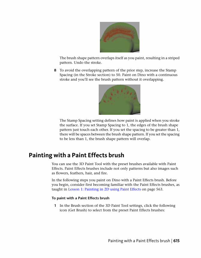
The brush shape pattern overlaps itself as you paint, resulting in a stripedpattern. Undo the stroke.
8 To avoid the overlapping pattern of the prior step, increase the StampSpacing (in the Stroke section) to 50. Paint on Dino with a continuousstroke and you’ll see the brush pattern without it overlapping.
The Stamp Spacing setting defines how paint is applied when you strokethe surface. If you set Stamp Spacing to 1, the edges of the brush shapepattern just touch each other. If you set the spacing to be greater than 1,there will be spaces between the brush shape pattern. If you set the spacingto be less than 1, the brush shape pattern will overlap.
Painting with a Paint Effects brushYou can use the 3D Paint Tool with the preset brushes available with PaintEffects. Paint Effects brushes include not only patterns but also images suchas flowers, feathers, hair, and fire.
In the following steps you paint on Dino with a Paint Effects brush. Beforeyou begin, consider first becoming familiar with the Paint Effects brushes, astaught in Lesson 1: Painting in 2D using Paint Effects on page 563.
To paint with a Paint Effects brush
1 In the Brush section of the 3D Paint Tool settings, click the followingicon (Get Brush) to select from the preset Paint Effects brushes:
Painting with a Paint Effects brush | 615

The Visor window opens. The Visor organizes the hundreds of PaintEffects brushes into category folders.
2 Scroll to the watercolor folder and click it.
To the right, swatch pictures of the Paint Effects brushes appear for thiscategory.
3 Select the spatterLight.mel brush. (To see the names of the swatches, dragthe pointer over them.)
Leave the Visor window open, but move it so you can see Dino again.
If you are using a tablet and stylus, you need to turn on Stylus Pressureagain to see the effect of your pressure as you paint. Stylus Pressure is offbecause you changed from the Artisan brush to a Paint Effects brush.
For Paint Effects brushes, the pressure you apply to the pen affects threedifferent settings. If you change the settings, it affects only the selectedbrush. The settings for each brush are separate from each other.
4 Paint on Dino.
5 In the Brush section of the 3D Paint Tool settings, click the followingicon (Edit Template Brush) to modify other brush settings:
The Paint Effects Brush Settings window opens. Any changes you maketo the settings in this window affect the display of your next stroke. Asan example, you’ll increase the brush’s incandescence.
616 | Chapter 11 Painting
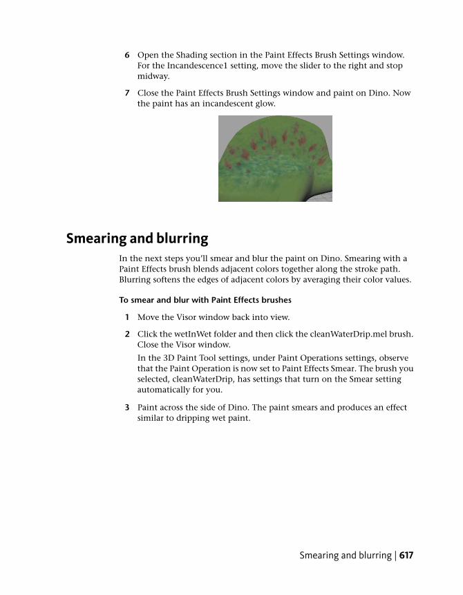
6 Open the Shading section in the Paint Effects Brush Settings window.For the Incandescence1 setting, move the slider to the right and stopmidway.
7 Close the Paint Effects Brush Settings window and paint on Dino. Nowthe paint has an incandescent glow.
Smearing and blurringIn the next steps you’ll smear and blur the paint on Dino. Smearing with aPaint Effects brush blends adjacent colors together along the stroke path.Blurring softens the edges of adjacent colors by averaging their color values.
To smear and blur with Paint Effects brushes
1 Move the Visor window back into view.
2 Click the wetInWet folder and then click the cleanWaterDrip.mel brush.Close the Visor window.
In the 3D Paint Tool settings, under Paint Operations settings, observethat the Paint Operation is now set to Paint Effects Smear. The brush youselected, cleanWaterDrip, has settings that turn on the Smear settingautomatically for you.
3 Paint across the side of Dino. The paint smears and produces an effectsimilar to dripping wet paint.
Smearing and blurring | 617

4 In the Paint Operations section of the 3D Paint Tool settings, select PaintEffects Blur.
This selects the default Paint Effects Blur brush.
5 Paint across the side of Dino to see the effect of Blur.
Painting a bump map textureNext, you’ll paint a bump pattern on Dino. In Maya, a bump texture createsthe illusion of surface relief. It does this by perturbing the surface normals tomake the surface appear bumpy. This is useful for making Dino’s skin appearmore “reptile-like”.
To paint a bump map texture
1 In the 3D Paint Tool window, click Reset Tool to return to the defaultsettings.
2 In the File Textures section, set the Attribute to Paint setting to BumpMap.
3 Click Assign/Edit Textures.
The Assign/Edit Textures window appears.
618 | Chapter 11 Painting

Earlier in the lesson, your painting affected only the Color attribute. Topaint bumps, it’s necessary to select a BumpMap as the new attribute youwant to paint, and then assign a new texture for the bumps you’ll create.
4 In the Assign/Edit Textures window, set both Size X and Size Y to 512and then click Assign/Edit Textures.
Maya creates a file texture and applies it to the Bump Map attribute ofthe DinoSkin material.
In the scene view, Dino’s color changes to white. Bump map textures arebased on grayscale colors. By default, when you create a rendered image,bumps will appear in the areas of the surface where there is significantgrayscale color contrast. For instance, if a region has black and whitestripes, you’ll see grooves there. Regions with little or no contrast displayno bump.
The bumps will not show in the scene view; you must create a renderedimage in order to see them. The same is true when you paint certain otherattributes, such as Transparency and Incandescence.
Before you paint bumps on Dino, you must set up the Maya panels soyou can interactively see the results of your strokes in a rendered image.
5 Select Panels > Layouts > Two Panes Stacked.
6 In the bottom panel, select Panels > Panel > Render View.
Maya now displays the perspective view, the Render View, and the 3DPaint Tool settings. With this arrangement, you’ll be able to see yourstrokes render as you paint.
7 In the perspective view, move the camera to a close-up view of Dino’sside.
8 In the Render View, select IPR > IPR Render > persp. This renders an imageof Dino in the Render View.
9 In the Render View, drag a selection box around Dino’s midsection andhump.
Painting a bump map texture | 619

This region will update when you paint.
For the IPR renderer to render bumps as you paint, you must update thebump map texture after each stroke. You can set this to occurautomatically.
10 In the File Textures section of the 3D Paint Tool settings, turn on Updateon Stroke.
For a grooved bump effect, you need to change the brush shape.
11 In the Brush section of the 3D Paint Tool settings, click the Browse button.
12 Select the hatch.jpg brush and click Open.
13 Paint on Dino’s side.
Notice the Render View updates with each stroke.
The bumps appear as grooves in Dino’s surface because you paintedcontrasting black stripes on the white texture. In general, gray or blackover a white background results in bumps that appear indented.
If you wanted bumps that appear raised on the surface, you could startwith a black background and paint gray or white over it. For example,you could flood the texture with a black Flood Color, then paint whiteor gray strokes rather than the default black.
Greater contrast between the background color and the color you paintresults in deeper-looking bumps. Less contrast results in more subtlebumps. In the previous step, you painted using a black color, resultingin prominent bumps. If you change the Color setting to a light gray andpaint on the white background, only subtle bumps will appear.
This concludes the lesson.
14 Before doing other lessons, restore the Channel Box in the Maya window.
620 | Chapter 11 Painting
15 Select Display > UI Elements > Channel Box/Layer Editor.
Beyond the lessonIn this lesson you were introduced to a few basic techniques related to the 3DPaint Tool. You learned how to:
■ Paint textures directly onto surfaces using the 3D Paint Tool.
■ Paint symmetrically onto surfaces.
■ Paint grey scale attributes to create bump texture effects.
There are several other capabilities in the Paint Operations section, such asthe Clone option for Artisan brushes. With the Clone option, you can duplicatethe color and pattern from an area of the texture and then paint that patternelsewhere on the texture. For details on these options and other 3D Paint Tooltechniques, refer to the Maya Help.
Location of 3D Paint Tool file textures
If you need to move or rename a file texture that Maya creates from yourpainting, look in the 3dPaintTextures directory under the current projectdirectory. If you paint an existing file texture that you created previously, forexample, with a paint program, Maya creates a copy and stores it in the3dPaintTextures directory.
Preparing UVs for painting
In this lesson you worked with a polygonal model that was specially preparedfor painting in this lesson. To paint successfully on a polygonal or subdivisionsurface, you must set up the surface UVs beforehand. UVs are points positionedaround the surface like vertices. They control how Maya stretches a texturearound a surface. For polygons and subdivision surfaces, you must arrangethe UVs so that textures—including the ones you paint with the 3D PaintTool—look correct when applied to the surface material. (The UVs on NURBSsurfaces are automatically arranged for you, so you do not have to changethem.)
You view and edit UVs using the UV Texture Editor (Window menu). You canobtain an introduction to UVs and the UV Texture Editor by completing theUV Texture Mapping lesson in this book. You can also learn more about UVsin the Maya Help by referring to the sections on Polygonal and Subdivisionssurfaces.
Beyond the lesson | 621

If you already have experience with editing UVs, remember these tworequirements for 3D painting:
■ UVs must not overlap.
■ UVs must fit with the 0 to 1 texture coordinates.
This illustration shows the UV Texture Editor with the UVs for the Dino modelused in this lesson. These UVs meet the above two requirements. Notice thatthe UVs form several meshes; they do not need to be one solid mesh.
Painting in Screen Projection mode
When you paint on a model, the brush follows the contours of the surface.This typically produces the most desirable results. However, this defaultbehavior leads to uneven paint application in some situations. A commonexample is along the line where two surfaces join together. It can also occurif the UVs are not arranged correctly, as described previously.
The solution to these situations is to turn on Screen Projection in the 3D PaintTool settings. Screen Projection applies paint as if you are projecting cinematicfilm onto a screen. Paint appears where the projection strikes the surface.
The following figure shows an example of this situation with a Paint Effectsbrush.
622 | Chapter 11 Painting
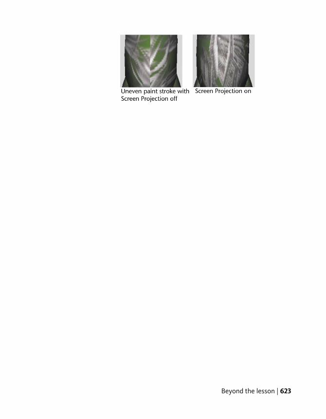
Beyond the lesson | 623

624
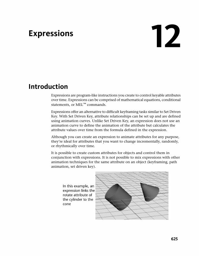
Expressions
IntroductionExpressions are program-like instructions you create to control keyable attributesover time. Expressions can be comprised of mathematical equations, conditionalstatements, or MEL™ commands.
Expressions offer an alternative to difficult keyframing tasks similar to Set DrivenKey. With Set Driven Key, attribute relationships can be set up and are definedusing animation curves. Unlike Set Driven Key, an expression does not use ananimation curve to define the animation of the attribute but calculates theattribute values over time from the formula defined in the expression.
Although you can create an expression to animate attributes for any purpose,they’re ideal for attributes that you want to change incrementally, randomly,or rhythmically over time.
It is possible to create custom attributes for objects and control them inconjunction with expressions. It is not possible to mix expressions with otheranimation techniques for the same attribute on an object (keyframing, pathanimation, set driven key).
12
625

This chapter contains the following lessons:
■ Lesson 1 Creating a simple expression: Introduction on page 627
■ Lesson 2 Conditional expressions: Introduction on page 634
■ Lesson 3 Controlling particle attributes: Introduction on page 643
Preparing for the lessonsTo ensure the lessons work as described, do these steps before beginning:
1 Select File > New Scene to create a new scene.
2 If you have not already done so, copy the GettingStarted folder fromits installation location to your projects directory. Then, set theGettingStarted directory as your Maya project. For more information,see Copying and setting the Maya project on page 25.
3 Select Window > Settings/Preferences > Preferences. Click the Settingscategory and set the Time option to Film (24 fps) so your animation playsat the default rate of 24 frames per second. Click the Timeline categoryand enter 0 and 300 for the Playback Start/End values. (Press the Enter(Windows and Linux) or Return (Mac OS X) as necessary.) Set the PlaybackSpeed to Play every frame. Click the Save button in the Preferenceswindow.
At this playback speed and frame range, the animation results of theexpressions you’ll create in the lessons will be easier to examine andunderstand.
4 With the pointer in the perspective view, press 5 (for Shading > SmoothShade All). It’s easier to see the expression effects on shaded objects thanwireframe objects in the following lessons.
626 | Chapter 12 Expressions

Lesson 1: Creating a simple expression
IntroductionThis lesson introduces you to some basic concepts regarding the creation andediting of expressions. You learn how to:
■ Use the expression editor to create and edit expressions.
■ Control both single and multiple attributes of objects in your scene.
Creating expressions to control a single attributeIn the following steps, you create a default sphere and write an expression toincrease its Scale Y attribute as the animation time increases during playback.
To create an expression
1 Make sure you’ve done the steps in Preparing for the lessons on page 626.
2 Create a NURBS or polygonal sphere with an X scale, Y scale, and Z scaleequal to 1. Rename the sphere Ball. (Upper and lower case text isimportant)
3 With Ball selected, choose Window > Animation Editors > ExpressionEditor.
4 In the Expression Name box, you can optionally enter an expressionname, for instance, ScaleBallHeight.
If you write several expressions in the same scene, giving each a namemight make it easier to find the desired expression if you decide to alterit later. If you don’t provide a name, the expression receives a defaultname, for instance, expression1.
Lesson 1: Creating a simple expression | 627
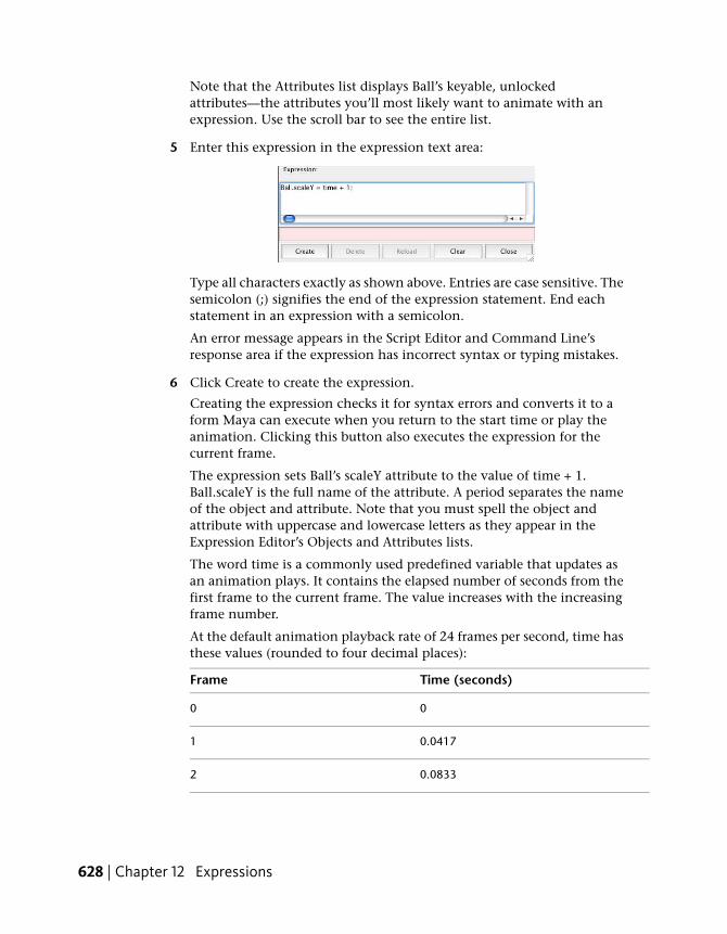
Note that the Attributes list displays Ball’s keyable, unlockedattributes—the attributes you’ll most likely want to animate with anexpression. Use the scroll bar to see the entire list.
5 Enter this expression in the expression text area:
Type all characters exactly as shown above. Entries are case sensitive. Thesemicolon (;) signifies the end of the expression statement. End eachstatement in an expression with a semicolon.
An error message appears in the Script Editor and Command Line’sresponse area if the expression has incorrect syntax or typing mistakes.
6 Click Create to create the expression.
Creating the expression checks it for syntax errors and converts it to aform Maya can execute when you return to the start time or play theanimation. Clicking this button also executes the expression for thecurrent frame.
The expression sets Ball’s scaleY attribute to the value of time + 1.Ball.scaleY is the full name of the attribute. A period separates the nameof the object and attribute. Note that you must spell the object andattribute with uppercase and lowercase letters as they appear in theExpression Editor’s Objects and Attributes lists.
The word time is a commonly used predefined variable that updates asan animation plays. It contains the elapsed number of seconds from thefirst frame to the current frame. The value increases with the increasingframe number.
At the default animation playback rate of 24 frames per second, time hasthese values (rounded to four decimal places):
Time (seconds)Frame
00
0.04171
0.08332
628 | Chapter 12 Expressions

Time (seconds)Frame
0.1253
1.024
10.0240
You can find the time elapsed in the animation at any frame bycalculating this formula with a desktop calculator:
For example, if the frame rate is 24 frames/second and the animation isat frame 1, the elapsed time is 1 divided by 24, or 0.0417. At frame 6, theelapsed time is 6 divided by 24, which equals 0.25. Note that if your framerate was 30 frames/second the calculated values would be different.
7 Go to the start time and play the animation. Ball’s scaleY attributeincreases as the time increases:
Ball.scaleY (time + 1)Time (seconds)Frame
100
1.04170.04171
1.08330.08332
1.1250.1253
2.01.024
11.010.0240
Maya executes the expression each frame. This causes the object size toscale along its Y-axis, stretching its height during playback.
Creating expressions to control a single attribute | 629

To see the value of Ball’s scaleY attribute at any particular frame, selectBall, display the Channel Box, and stop the animation at the desiredframe. The Channel Box updates its values after you stop the animation.
The scaling is smooth because the geometry stretches in synch with thesmall time increments of the animation playback.
8 Close the Expression Editor window.
Editing expressionsTo edit an expression after you’ve created it and closed the window, you mustknow how to find the expression in the Expression Editor. The next stepsshow how to find and edit the expression. Specifically, you’ll change theexpression to alter how quickly the scaleY value changes.
To edit the expression
1 To display the Expression Editor again, select Window > Animation Editors> Expression Editor.
2 To find the expression, make sure the Ball is selected. In the Attributeslist of the Expression Editor, select scaleY, the attribute controlled by theexpression.
If you don’t see the scaleY attribute, scroll through the Attributes list asnecessary. You can also use the Select Filter menu option to customizehow you search for your expressions within the Expression Editor.
The expression you created previously appears in the expression textfield:
Ball.scaleY = time + 1;
3 Change the expression to this:
Ball.scaleY = time/5 + 1;
By dividing time by 5, you’ll make the Y scaling increase one-fifth as fastas with the previous version of the expression.
Note that you can use the keyboard commands Ctrl-c (Windows andLinux) or Control-c (Mac OS X), Ctrl-x or Control-x, and Ctrl-v orControl-v to copy, cut, and paste text in the Expression Editor andelsewhere in Maya.
4 Click Edit to update the modified expression.
630 | Chapter 12 Expressions

Clicking the Edit button does the same action as clicking the Createbutton. The Create button exists only for new expressions. The Edit buttonreplaces the Create button when you display an existing expression.
5 Play the animation to see the results of the new expression.
The sphere scales at a slower rate than before.
6 Stop the animation and go to the start time.
7 At this point and in subsequent steps, save the scene if you think you’llwant to examine it at a later date.
Using expressions to control multiple attributesYou can change the expression to control two or more attributes of Ball as inthis example:
Ball.scaleX = time/2 +1;
Ball.scaleY = time/3 +1;
Ball.scaleZ = time/5 +1;
Maya scales the Ball at different rates for the X, Y, and Z dimensions.
Linking multiple attributes on the same objectYou can change the expression to link the value of one attribute to anotheras in this example:
Ball.scaleX = time + 1;
Ball.scaleY = Ball.scaleX;
Ball.scaleZ = Ball.scaleX;
The second statement sets Ball.scaleY to the value of Ball.scaleX. Becauseyou’ve set Ball.scaleX to the value of time + 1, Ball.scaleY also has the valueof time + 1. You’re linking one attribute’s value to another. The third statementalso sets Ball.scaleZ to the value of the attribute Ball.scaleX.
The advantage of this expression is that if you assign a different value toBall.scaleX in the first statement, the second and third statements automaticallyreceive the new value.
Using expressions to control multiple attributes | 631

Controlling attributes in two objectsYou can add an object to the scene and use the expression to control any ofits attributes also. For example, suppose you added a default NURBS orpolygonal cylinder named Drum to the scene. You could control the attributesof Ball and Drum with the same expression as in this example:
Ball.scaleY = time/2 + 1;
Drum.scaleX = time + 1;
Drum.scaleY = time + 1;
You can link attributes in different objects—so a change in one attribute altersthe behavior of the other. For example, you could cause Drum’s scaleY valueto always equal two times Ball’s scaleY value as in this example:
Ball.scaleY = time + 1;
Drum.scaleY = Ball.scaleY * 2;
If you decide to control attributes in two (or more) objects, you can selecteither object to write the expression. In fact, any object or node in a scenecan be selected when you write an expression to control an object other thana particle object.
Alternatively, you can write two (or more) expressions, for instance, one thatcontrols Ball.scaleY and one that controls Drum.scaleX and Drum.scaleY.
The advantage of creating separate expressions is that you’ll have twoexpression names, each presumably named after the object and attribute you’recontrolling. Having two expression names makes it easier to find the expressionthat controls the desired attribute.
The advantage of using a single expression to control the attributes is that allstatements are in a single expression. You don’t need to edit two expressions.
Beyond the lessonIn this lesson you learned how to:
■ Create and edit simple expressions using the Expression Editor.
■ Use variables, for example time, to control the specific attributes withinexpressions.When you write expressions, it is common to assign the built-in timevariable to an attribute so the attribute value predictably increases as theanimation plays. It’s also useful to link an attribute’s value to the value of
632 | Chapter 12 Expressions
another attribute, such as setting the ball’s scale Y and Z attributes to equalthe scale X value.
■ Control multiple attributes with a single expression.Your expressions can control multiple attributes of the same object or ofmultiple objects. Alternatively, you can write a single expression for eachattribute or object.
For more information on the various mathematical operators that arepossible with expressions, refer to the Maya Help.
Behind the lesson
Although not shown in the lessons, you can decrease an attribute value duringplayback by subtracting time from some number. Example:
Ball.scaleY = 3 - time;
This decreases the value of Ball’s scaleY attribute for the first three seconds ofplayback.
When you use the predefined time variable, note the animation start framevalue. The lessons in this chapter use a start time of 0. In your work, you mightcreate an animation with a start time of 1. With Maya’s default frame rate of24 frames per second, time is 0.0417 at frame 1.
Because of this small time offset from 0, the prior lesson would have requiredmore steps and instructions to work with frame 1 as the start time. For instance,suppose you use following expression with the start time at 1.
Ball.scaleY = time + 1;
If you go to the start time, the expression sets the initial value of Ball’s scaleYattribute to time + 1, which equals 0.0417 + 1, or 1.0417. Because Ball’s scaleYattribute was 1 when you created it, going to the start time sets scaleY to avalue 0.0417 larger than its initial value.
This discrepancy means the Ball scaleY is larger than its scaleX and scaleZattributes in the first frame of the animation. Although the difference is minorin this example, other cases might be more significant.
To start your animation at frame 1 and get the same result as the example,you can subtract 0.0417 from the attribute:
Ball.scaleY = (time - 0.0417) + 1;
When you go to the start time, the expression sets Ball’s scaleY value to (0.0417- 0.0417) + 1. This equals 1, its original scaleY value.
Beyond the lesson | 633
Lesson 2: Conditional expressions
IntroductionConditional statements set one attribute or variable for an expression basedon the condition of another attribute or variable. This means that when aparticular defined condition exists for one attribute then another attribute ischanged based on how the expression defines it to do so.
In this lesson you learn how to:
■ Use conditional statements to control an expression.
■ Refine the conditional statements using if and else statements.
Creating a conditional expressionIn the following steps, you create a default sphere and write an expression toincrease its Scale Y attribute based on the animation playback time. In thefirst two seconds of the animation time, Scale Y increases with the value ofthe time. At two seconds and thereafter, Scale Y no longer increases.
To create an expression using conditional statements
1 Make sure you’ve done the steps in Preparing for the lessons on page 626.
2 Create a NURBS or polygonal sphere at the origin with an X scale, Y scale,and Z scale of 1.
3 Name the sphere Balloon.
4 Go to the start time.
5 With Balloon selected, choose Window > Animation Editors > ExpressionEditor.
6 Enter this expression:
if (time < 2)
Balloon.scaleY = time;
This expression is an if statement. The if keyword causes the expressionto make a decision based on a comparison of two or more items. In thiscase, the expression compares the value of time to the value 2.
634 | Chapter 12 Expressions
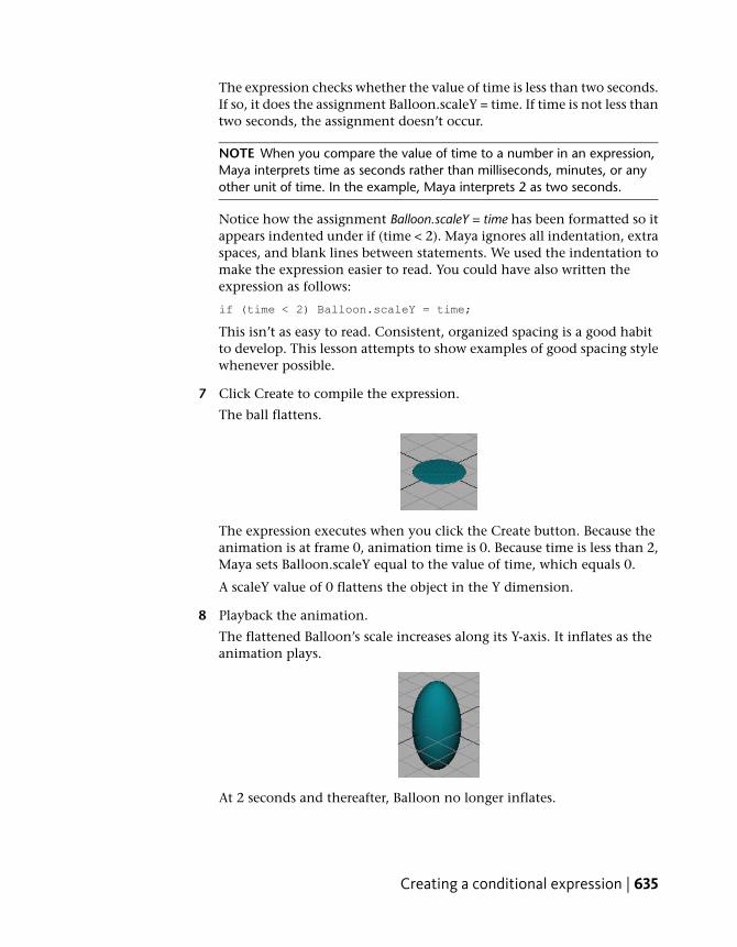
The expression checks whether the value of time is less than two seconds.If so, it does the assignment Balloon.scaleY = time. If time is not less thantwo seconds, the assignment doesn’t occur.
NOTE When you compare the value of time to a number in an expression,Maya interprets time as seconds rather than milliseconds, minutes, or anyother unit of time. In the example, Maya interprets 2 as two seconds.
Notice how the assignment Balloon.scaleY = time has been formatted so itappears indented under if (time < 2). Maya ignores all indentation, extraspaces, and blank lines between statements. We used the indentation tomake the expression easier to read. You could have also written theexpression as follows:
if (time < 2) Balloon.scaleY = time;
This isn’t as easy to read. Consistent, organized spacing is a good habitto develop. This lesson attempts to show examples of good spacing stylewhenever possible.
7 Click Create to compile the expression.
The ball flattens.
The expression executes when you click the Create button. Because theanimation is at frame 0, animation time is 0. Because time is less than 2,Maya sets Balloon.scaleY equal to the value of time, which equals 0.
A scaleY value of 0 flattens the object in the Y dimension.
8 Playback the animation.
The flattened Balloon’s scale increases along its Y-axis. It inflates as theanimation plays.
At 2 seconds and thereafter, Balloon no longer inflates.
Creating a conditional expression | 635

When time equals 2 or more, the if condition is no longer true. Thestatement that follows it, Balloon.scaleY = time, no longer executes. Thevalue of the scaleY attribute stays at the last value it had before timebecame 2, specifically, 1.9583.
Recall that this example uses a frame rate of 24 frames per second. Thetime and Balloon.scaleY have these values at various frames:
Balloon.scaleY (time)Time (seconds)Frame
000
0.04170.04171
0.08330.08332
0.1250.1253
1.01.024
1.95831.9647
1.95832.048
1.95832.0449
The if statement’s condition, (time < 2), is a comparison. The conditionmust be surrounded by parentheses to isolate it from assignment thatfollows it.
The < in the condition is a relational operator. A relational operator testshow one value relates to another. In the example, the < tested whethertime is less than 2.
Besides the < operator shown in this example, there are several otherrelational operators such as >, >=, ==, and so on. See the Maya Help formore details.
9 Stop the animation and go to the start time. Balloon flattens again becausethe scaleY attribute becomes 0 when you go to the start time. Time is 0,so scaleY is 0.
636 | Chapter 12 Expressions

Other conditional statement optionsYou can make Balloon rise after it inflates by adding another if statement tothe expression.
To add an if statement to the expression
1 Change the expression to this:
if (time < 2)
Balloon.scaleY = time;
if (time >= 2)
Balloon.translateY = time;
2 Click Edit to compile the expression.
3 Play the animation.
Balloon inflates for two seconds. After two seconds, Balloon stops inflatingand its position skips from a Y-axis position of 0 to 2. You’ll eliminatethe motion skip in a later step.
The new if statement increases the translateY position of Balloon afterthe animation time rises above two seconds. The >= symbols mean greaterthan or equal to. Whenever time is greater than or equal to 2, theexpression assigns Balloon’s translateY the value of time. The translateYvalue therefore increases for the rest of your animation’s playback range.
Notice that a semicolon ends each statement for a particular condition.Forgetting a semicolon after each statement causes a syntax error, andthe changes you’ve made to the expression won’t take effect.
NOTE Always examine the Script Editor for error messages after you edit anexpression and click the Create button. If you alter a previously successfulexpression and a syntax error occurs, Maya executes the previous successfulexpression when you play the animation. This might make you believe yourchanges took effect. Error messages are preceded by the text // Error:.
4 Stop the animation and go to the start time. Balloon flattens but doesn’treturn to the origin. (If Balloon has risen out of view, adjust your camerato see it.)
Balloon doesn’t return to the origin because the expression doesn’t assignBalloon a starting point for the beginning of the animation.
Other conditional statement options | 637

5 To make Balloon return to the origin, change the expression to this:
if (time < 2)
Balloon.translateY = 0;
if (time < 2)
Balloon.scaleY = time;
if (time >= 2)
Balloon.translateY = time;
The new first statement sets Balloon.translateY to 0 whenever time is lessthan 2.
Note that you can put the three statements in any order in this example.When Maya plays each frame, it executes each statement in the expressionin the order listed. In this example, the statements work independently,so their order doesn’t matter.
We put the statements in the order of time execution because it’s easierto see the logic of the expression. If you ever need to change theexpression, you’ll be able to grasp the expression’s actions more quickly.
6 Click Edit.
7 Stop the animation and go to the start time.
The flattened Balloon returns to its correct position at the origin.
8 Play the animation.
Balloon inflates for two seconds, then rises. As it rises, it jumps slightlyhigher at approximately frame 48.
638 | Chapter 12 Expressions
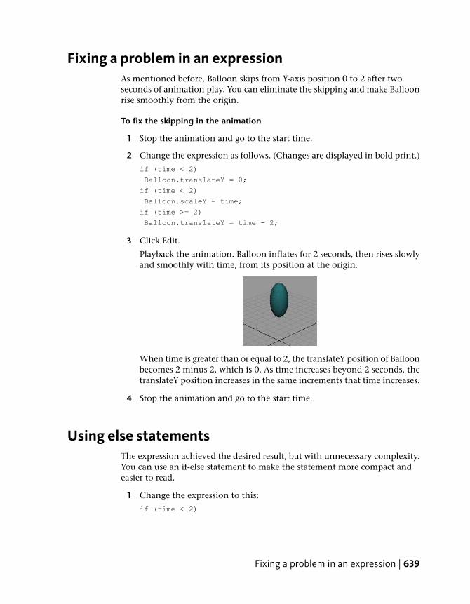
Fixing a problem in an expressionAs mentioned before, Balloon skips from Y-axis position 0 to 2 after twoseconds of animation play. You can eliminate the skipping and make Balloonrise smoothly from the origin.
To fix the skipping in the animation
1 Stop the animation and go to the start time.
2 Change the expression as follows. (Changes are displayed in bold print.)
if (time < 2)
Balloon.translateY = 0;
if (time < 2)
Balloon.scaleY = time;
if (time >= 2)
Balloon.translateY = time - 2;
3 Click Edit.
Playback the animation. Balloon inflates for 2 seconds, then rises slowlyand smoothly with time, from its position at the origin.
When time is greater than or equal to 2, the translateY position of Balloonbecomes 2 minus 2, which is 0. As time increases beyond 2 seconds, thetranslateY position increases in the same increments that time increases.
4 Stop the animation and go to the start time.
Using else statementsThe expression achieved the desired result, but with unnecessary complexity.You can use an if-else statement to make the statement more compact andeasier to read.
1 Change the expression to this:
if (time < 2)
Fixing a problem in an expression | 639
Balloon.translateY = 0;
if (time < 2)
Balloon.scaleY = time;
else
Balloon.translateY = time - 2;
2 Click Edit.
3 Play the animation.
The animation plays back exactly as before.
This additional variation on the if conditional statement includes theelse statement. It is used as an option when the if statement condition isnot true. The else keyword sets Balloon.translateY to time - 2 when (time< 2) is false. In English terms, the combination of the if and elsestatements means: If time is less than two seconds, set Balloon.scaleY tothe value of time. Otherwise (when time is greater than or equal to twoseconds), set Balloon.translateY to time minus two.
At any instant in the animation’s playback, either Balloon.scaleY = timeexecutes or Balloon.translateY = time - 2 executes. Under no circumstancescan they both execute. The else statement executes only when the ifcondition that precedes it is false.
The first if statement executes whenever time equals 0. It is unrelated tothe if-else statements.
Using else statements instead of multiple if statements makes anexpression simpler to read. If you use an if-else construction instead of alengthy list of if statements, you’ll also improve the execution speed ofthe expression. This improves your animation’s playback and renderingspeed.
Either expression is valid. If using the if-else construction seems confusing,stick with multiple if statements.
You can accomplish most expression animation tasks with several ifstatements strung after one another.
4 Stop the animation and go to the start time.
Simplifying expressionsYou can simplify the expression to make it easier to read.
1 Change the expression to this:
640 | Chapter 12 Expressions

if (time < 2)
{
Balloon.translateY = 0;
Balloon.scaleY = time;
}
else
Balloon.translateY = time - 2;
We removed the second if statement:
if (time < 2)
In its place, we enclosed the remaining statements with braces { and }.Maya evaluates both the statements between the braces if the condition(time < 2) is true. Setting Ball.translateY to 0 here instead of in a separateif statement makes the expression easier to read and comprehend.Reducing the statement in this way also makes it more efficient for Mayato process and easier to troubleshoot if you encounter a problem.
Note that you can put multiple statements between braces for an elsestatement, just as you do for an if statement.
2 Click Edit.
3 Play the animation.
The animation plays exactly as before with the new expression.
4 Stop the animation and go to the start time.
Editing expressions to refine an animationYou can further refine the animation by expanding Balloon more slowly.
To edit the expression to scale the balloon more slowly
1 Change the expression to this:
if (time < 2)
{
Balloon.translateY = 0;
Balloon.scaleY = time * 0.6;
}
else
Balloon.translateY = time - 2;
(The asterisk (*) multiplies time by 0.6.)
2 Click Edit.
Editing expressions to refine an animation | 641
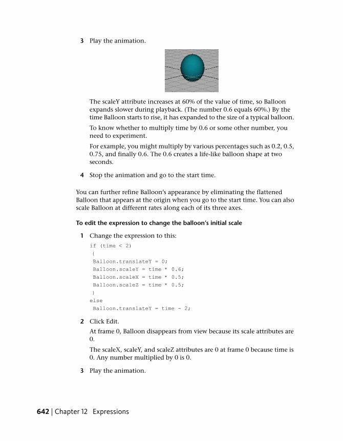
3 Play the animation.
The scaleY attribute increases at 60% of the value of time, so Balloonexpands slower during playback. (The number 0.6 equals 60%.) By thetime Balloon starts to rise, it has expanded to the size of a typical balloon.
To know whether to multiply time by 0.6 or some other number, youneed to experiment.
For example, you might multiply by various percentages such as 0.2, 0.5,0.75, and finally 0.6. The 0.6 creates a life-like balloon shape at twoseconds.
4 Stop the animation and go to the start time.
You can further refine Balloon’s appearance by eliminating the flattenedBalloon that appears at the origin when you go to the start time. You can alsoscale Balloon at different rates along each of its three axes.
To edit the expression to change the balloon’s initial scale
1 Change the expression to this:
if (time < 2)
{
Balloon.translateY = 0;
Balloon.scaleY = time * 0.6;
Balloon.scaleX = time * 0.5;
Balloon.scaleZ = time * 0.5;
}
else
Balloon.translateY = time - 2;
2 Click Edit.
At frame 0, Balloon disappears from view because its scale attributes are0.
The scaleX, scaleY, and scaleZ attributes are 0 at frame 0 because time is0. Any number multiplied by 0 is 0.
3 Play the animation.
642 | Chapter 12 Expressions

As time increases, the value of Balloon’s scale attributes increase.
Because the expression sets scaleX and scaleZ to 50% of the value of time,these dimensions scale slower than scaleY, which is set to 60% of thevalue of time. Balloon scales faster in height than in width or depth. Thisis true for many real balloons.
4 Stop the animation and go to the start time.
5 Save the scene if you plan to examine it later.
Beyond the lessonIn this lesson you learned how to:
■ Use conditional statements to control an expression.You can accomplish many expression tasks with several if statements strungafter one another. However, using else statements instead of multiple ifstatements makes an expression simpler to read.
If statements and else statements are two of the most common programmingfeatures available in expressions. If you’re familiar with programming, youcan write expressions with an extensive syntax similar to the C language.
For further information and related techniques, refer to the Maya Help.
Lesson 3: Controlling particle attributes
IntroductionYou can use an expression to control attributes of particle objects. Particleexpressions can be more complex than other types of expressions. For example,
Beyond the lesson | 643

you can write an expression to control all particles in an object the same way,or you can control each particle differently.
In this lesson you learn how to:
■ create a particle object
■ create a creation expression to set the initial color of the particles
■ create a runtime expression to control the color during playback
■ use a random function to randomize how the color changes
■ control the timing of an expression
Creating particle objectsIn the following steps, you’ll create a particle object made of 100 randomlypositioned particles displayed as tiny spheres. You’ll also dynamically add anattribute to the particles. To color particles with an expression, Maya requiresyou to dynamically add the appropriate attribute.
To create a particle object
1 Make sure you’ve done the steps in Preparing for the lessons on page 626.
2 From the Dynamics menu set, select Particles > Particle Tool > .
3 In the Tool Settings window, click Reset Tool, and set the followingoptions:
■ Particle Name: Bubbles
■ Number of Particles: 100
■ Maximum Radius: 5
■ Click in the scene view (roughly in the center) to create the100-particle object.
4 From the Toolbox, select the Selection Tool so that particles becomeselected.
5 With Bubbles selected, display the Attribute Editor.
644 | Chapter 12 Expressions
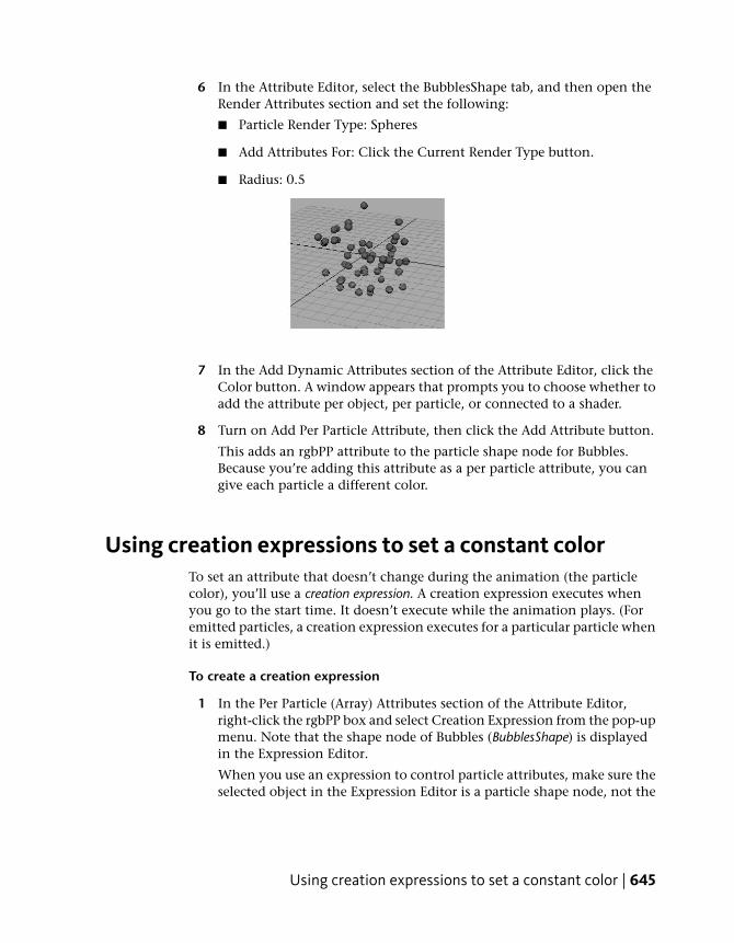
6 In the Attribute Editor, select the BubblesShape tab, and then open theRender Attributes section and set the following:
■ Particle Render Type: Spheres
■ Add Attributes For: Click the Current Render Type button.
■ Radius: 0.5
7 In the Add Dynamic Attributes section of the Attribute Editor, click theColor button. A window appears that prompts you to choose whether toadd the attribute per object, per particle, or connected to a shader.
8 Turn on Add Per Particle Attribute, then click the Add Attribute button.
This adds an rgbPP attribute to the particle shape node for Bubbles.Because you’re adding this attribute as a per particle attribute, you cangive each particle a different color.
Using creation expressions to set a constant colorTo set an attribute that doesn’t change during the animation (the particlecolor), you’ll use a creation expression. A creation expression executes whenyou go to the start time. It doesn’t execute while the animation plays. (Foremitted particles, a creation expression executes for a particular particle whenit is emitted.)
To create a creation expression
1 In the Per Particle (Array) Attributes section of the Attribute Editor,right-click the rgbPP box and select Creation Expression from the pop-upmenu. Note that the shape node of Bubbles (BubblesShape) is displayedin the Expression Editor.
When you use an expression to control particle attributes, make sure theselected object in the Expression Editor is a particle shape node, not the
Using creation expressions to set a constant color | 645

transform node of the particle object. If a particle object’s transform nodeis selected, move the mouse pointer to the scene view and press the downarrow key to select the particle shape node.
2 Enter this expression and then click the Create button:
BubblesShape.rgbPP = <<1,0,0>>;
When you click the Create button in the Expression Editor, Maya checksthe syntax of the expression. Assuming you made no typing errors, theexpression executes once for each of the 100 particles.
The expression colors all particles in the object red. The double anglebrackets << and >> enclose a vector that sets the red, green, and bluecomponents of the rgbPP attribute to 1, 0, and 0. In the RGB color scheme,this gives the object a red color.
If the particles are uncolored, check that you’ve turned on Shading >Smooth Shade All. This shading mode is necessary for particles to showthe color assigned in an expression.
3 Play the animation. The particles remain red.
Using runtime expressionsThere is one other type of expression you can create for a particle object (shapenode)—a runtime expression. By default, a runtime expression executes eachframe during playback. A runtime expression does not execute when you goto the start time (or at the time in which a particle is emitted).
You’ll often create both types of expressions for a particle object—a creationexpression that initializes an attribute value in the first frame, and a runtimeexpression that controls the attribute value in subsequent frames.
The following steps show how to create a runtime expression to change particlecolor during playback.
646 | Chapter 12 Expressions

To create a runtime expression
1 In the Per Particle (Array) Attributes section of the Attribute Editor,right-click the rgbPP box and select Runtime Before Dynamics Expressionfrom the pop-up menu.
2 Enter this runtime expression:
BubblesShape.rgbPP = sphrand(1);
3 Click the Create button to compile the expression.
4 Play the animation.
The particles flicker in random colors as the animation plays back. Theruntime expression controls the rgbPP attribute during playback. BecausergbPP is a per particle attribute, the runtime expression executes for eachparticle in the object for each frame. For each particle, the expressionassigns the rgbPP attribute the output from the execution of the sphrandfunction with an argument of 1. The sphrand function is one of Maya’smany built-in mathematical functions that are useful in expressions.
The sphrand function with an argument of 1 assigns each particle’s rgbPPcolor a random vector. The vector represents a random point in a sphericalregion of radius 1. The left, middle, and right rgbPP color componentsget a value no less than -1 and no greater than 1. (R, G, and B values lessthan 0 are treated as 0—a black color).
The sphrand function returns a different random vector each execution,so each particle receives a different random rgbPP value, and therefore,a different color. The color changes each frame.
5 Rewind and play the animation again.
The particles become red when you go to the start time, and randomcolors during playback.
Using runtime expressions | 647

NOTE You can use only one creation and one runtime expression per particleobject (shape node) in your scene. To control multiple attributes of a singleparticle object, you must do so within one creation expression and oneruntime expression. You can’t create a separate expression for each attributeas you can for other types of objects. You therefore don’t need to select anattribute from the Expression Editor’s Attributes list.
Modifying runtime expressionsYou might have trouble seeing the color of a particle in any instant becausethe color changes so quickly. You can slow the change of colors to create aflashing Christmas light effect. The following steps make the particles changecolors every second of animation.
To adjust the timing of the change of color
1 Change the runtime expression to this:
if ((frame % 24) == 0)
BubblesShape.rgbPP = sphrand(1);
This expression uses the modulus operator (%) to control when the rgbPPattribute of the particles receives a random color. The modulus operatorreturns the remainder after division. For example, 24 divided by 24 returns0, but 25 divided by 24 returns 1. (Dividing 25 by 24 equals 1 with aremainder of 1.)
If the value of frame divided by 24 is equal to any number with aremainder of 0, the assignment to BubblesShape.rgbPP occurs. In otherwords, the assignment occurs when frame equals 24, 48, 72, and so on.At an animation rate of 24 frames/second, the assignment happens onceeach second.
The == symbols mean is equal to. In conditional statements, be carefulto type == rather than =. The = symbol means assign the value to.
2 Rewind and play the animation again.
When you go to the start time, the particles turn red because the creationexpression executes. When the animation plays, the particles receive arandom color once each second.
648 | Chapter 12 Expressions
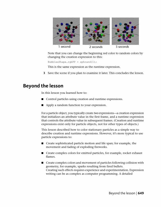
Note that you can change the beginning red color to random colors bychanging the creation expression to this:
BubblesShape.rgbPP = sphrand(1);
This is the same expression as the runtime expression.
3 Save the scene if you plan to examine it later. This concludes the lesson.
Beyond the lessonIn this lesson you learned how to:
■ Control particles using creation and runtime expressions.
■ Apply a random function to your expression.
For a particle object, you typically create two expressions—a creation expressionthat initializes an attribute value in the first frame, and a runtime expressionthat controls the attribute value in subsequent frames. (Creation and runtimeexpressions exist only for particle objects, not for other types of objects.)
This lesson described how to color stationary particles as a simple way todescribe creation and runtime expressions. However, it’s more typical to useparticle expressions to:
■ Create sophisticated particle motion and life span; for example, themovement and fading of exploding fireworks.
■ Create complex colors for emitted particles, for example, rocket exhaustflames.
■ Create complex colors and movement of particles following collision withgeometry, for example, sparks resulting from fired bullets.Creating such effects requires experience and experimentation. Expressionwriting can be as complex as computer programming. A detailed
Beyond the lesson | 649

understanding of expression execution and syntax is essential. You alsoneed to become familiar with the built-in mathematical functions such asthe sphrand function introduced in this lesson.
For further information and related techniques, refer to the Maya Help.
650 | Chapter 12 Expressions

Scripting in Maya
IntroductionScripting languages in Maya allow you to:
■ Automate repetitive or frequently performed tasks.You can write scripts to execute operations that would normally be selectedfrom the user interface or performed using tools and user manipulation.
■ Change Maya’s user interface.You can create windows and controls that affect objects in the scene.
■ Establish development standards.You can enforce naming conventions, workflows and model scales.
■ Create new tools and functions.You can extend Maya’s functionality in ways that help you do your work.
In this chapter, you learn some common scripting techniques and features thathighlight the capabilities of scripting in Maya:
■ Some basic concepts on page 652
■ Lesson 1 Commands in MEL: Introduction on page 656
■ Lesson 2 Saving scripts to the Shelf: Introduction on page 666
■ Lesson 3 Using Variables with MEL: Introduction on page 674
■ Lesson 4 Procedures and user interface creation: Introduction on page 683
■ Lesson 5 Using Python in Maya: Introduction on page 703
13
651
Some basic conceptsThe following section introduces some basic concepts that help you understandwhat’s going on when you use scripting in Maya.
The command architecture
Maya has a command-based architecture for handling all of its operations.The commands for all of Maya’s functionality are accessed through scriptinglanguage commands tied to the Maya user interface—menus, tools, dialogboxes; in fact, just about anything you interact with in Maya. As well, youcan explicitly enter Maya commands in the scripting languages that Mayasupports.
Every Maya command has multiple arguments that set the way in which thecommand executes. Arguments and their implicit or explicit values are requiredfor a command to execute.
To set argument values, the scripting languages in Maya use flags. Flags tellthe scripting language which argument of the Maya command is set withwhat value. The value that is assigned to the argument follows the flag.
Flags have short and long names in MEL and Python. Commands executeidentically whether or not you use the short or long name of the flag. Longnames are often descriptive and useful for new users; short names abbreviateflag names for power users.
Scripting languages in Maya
Maya supports two scripting languages:
■ MEL (Maya Embedded Language) is a proprietary scripting languagemodeled after Unix shell script.
■ Python is a recent addition to Maya that provides the same access to Maya’scommands as MEL. Python is a widely-used modern programminglanguage.
Maya’s user interface is built using scripts that execute (call) Maya commands.As Python is a recent addition to Maya, the majority of the scripts accessedthrough the user interface are written in MEL.
For example, when you click the sphere icon on the Shelf or select an itemfrom a menu, Maya calls MEL commands to create a sphere or execute thecommand associated with the menu item.
652 | Chapter 13 Scripting in Maya

Entering commands in Maya
There are several ways to explicitly enter scripting commands in Maya.
■ To enter single line MEL and Python commands, use the Command Line.To show the Command Line if it is hidden, select Display > UI Elements.The Command Line is located near the bottom edge of the Maya interface.
■ To enter multi-line MEL and Python commands, use the Script Editor. TheScript Editor displays a history of executed commands, as well as the resultsand outputs of commands. To open the Script Editor, select Window >General Editors > Script Editor.
■ As well, the Expression Editor uses a subset of MEL commands to createanimation in the scene. MEL commands in the Expression Editor areevaluated for every frame in the animation. The Expression Editor doesnot support Python commands. To open the Expression Editor, selectWindow > Animation Editors > Expression Editor.
You can also load external MEL and Python files and run them using the ScriptEditor. For more information, see Loading a script file on page 691.
What MEL looks like
Invoking commands in MEL has the basic structure of a command followedby a combination of flags and arguments. Flags are prefaced by the hyphencharacter in MEL.
All MEL commands are case-sensitive; SPHERE is not the same as sphere (andreturns an error message).
If no flags are provided, the command executes with default arguments. Thecommand fails if it requires arguments that it did not get.
Some basic concepts | 653
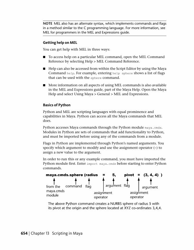
NOTE MEL also has an alternate syntax, which implements commands and flagsin a method similar to the C programming language. For more information, seeMEL for programmers in the MEL and Expressions guide.
Getting help on MEL
You can get help with MEL in three ways:
■ To access help on a particular MEL command, open the MEL CommandReference by selecting Help > MEL Command Reference.
■ Help can also be accessed from within the Script Editor by using the MayaCommand help. For example, entering help sphere shows a list of flagsthat can be used with the sphere command.
■ More information on all aspects of using MEL commands is also availablein the MEL and Expressions guide, part of the Maya Help. Open the MayaHelp and select Using Maya > General > MEL and Expressions.
Basics of Python
Python and MEL are scripting languages with equal prominence andcapabilities in Maya. Python can access all the Maya commands that MELdoes.
Python accesses Maya commands through the Python module maya.cmds.Modules in Python are sets of commands that add functionality to Python,and must be imported before using any of the commands from a module.
Flags in Python are implemented through Python’s named arguments. Youspecify which argument to modify and use the assignment operator (=) toassign a new value to the argument.
In order to run this or any example command, you must have imported thePython module first. Enter import maya.cmds before starting to enter Pythoncommands.
654 | Chapter 13 Scripting in Maya
All Python commands are case-sensitive; maya.cmds.SPHERE is not the sameas maya.cmds.sphere (and returns an error message).
Getting help on Python
You can get help with Python in several different ways:
■ To access help on a particular Maya (Python) command, open the PythonCommand Reference by selecting Help > Python Command Reference.
■ You can also access help on Maya Python commands from within theScript Editor by using the Maya Command help(). For example: typingmaya.cmds.help("sphere") outputs a list of possible flags that can be usedwith the sphere command.
■ Help for native Python commands is accessed from within the Script Editorby typing help("command") where command is the Python command youwant to access help for.
■ More information on using Python commands is also available in thePython guide, part of the Maya Help. Open the Maya Help and select UsingMaya > General > Python.
■ There are existing reference materials and documentation for Python onthe web, as well as many downloadable modules to add extra functionalityto Python.
■ Getting Started tutorials: http://www.python.org/about/gettingstarted
■ Python documentation: http://docs.python.org
■ Python modules: http://cheeseshop.python.org
Preparing for the lessonsTo ensure the lessons work as described, do these steps before beginning:
1 Select File > New Scene to create a new scene.
2 If you have not already done so, copy the GettingStarted folder fromits installation location to your projects directory. Then, set theGettingStarted directory as your Maya project. For more information,see Copying and setting the Maya project on page 25.
Preparing for the lessons | 655

3 Make sure the Construction History icon (below the menu bar) is on. (Ifit is turned off, it has a large X across it.)
4 Ensure that the interactive creation option for primitives is turned off byselecting Create > Polygon Primitives > Interactive Creation. The optionis off when a check mark does not display beside the item’s name in themenu.
5 Ensure that the interactive creation option for surfaces is turned off byselecting Create > NURBS Primitives > Interactive Creation. The optionis off when a check mark does not display beside the item’s name in themenu.
Lesson 1: Commands in MEL
Introduction
This lesson provides a brief introduction to using MEL scripting commands.In this lesson, you learn how to:
■ Use the Script Editor to view MEL command history
656 | Chapter 13 Scripting in Maya

■ Enter MEL commands in the Script Editor
■ Create geometry with MEL commands
■ Modify attributes of objects with MEL commands
■ Interpret Script Editor history
Entering MEL commandsYou can enter MEL commands in the Command Line or the Script Editor. TheCommand Line can only accept single line MEL commands, while the ScriptEditor provides a method to input multiple MEL commands and view theresults.
To use the Command Line to input MEL commands
1 Select Display > UI Elements.
Ensure that Command Line is checked.
2 Click in the Command Line text field to position the text cursor in thefield
By default the Command Line is in MEL script entry mode. You canchange the mode by clicking on the text in the lower left hand corner.For this lesson, ensure the Command Line is in MEL script entry mode.
3 Type the following in the Command Line.
sphere;
All MEL and Python entries are case sensitive.
4 To execute the command, press Enter on the numeric part of yourkeyboard, or press Ctrl+Enter.
5 A NURBS sphere is created at the origin.
Entering MEL commands | 657

In the Script Editor, the Enter (Windows and Linux) or Return (Mac OS X)key above the Shift key does not execute a command. It starts a new line soyou can type several commands before executing them.
Observing script historyThe Script Editor displays a running history of executed commands and theresults of commands that Maya executes. You can copy most commands fromthe history section of the Script Editor and paste them in the input section toexecute them.
To set up the Script Editor
➤ Select Window > General Editors > Script Editor.
The Script Editor window opens.
The lower half of the Script Editor is the input section where you enter scriptingcommands.
By default, Maya displays basic feedback from executed commands. However,when Echo All Commands is on, Maya shows all the history from a command,including when a script calls another script or modifies elements of the userinterface. While learning MEL, the extra lines of output produced when EchoAll Commands is on can be confusing because there is so much output. Asyou become more experienced in MEL, the extra lines of history can be usefulfor debugging a MEL script.
658 | Chapter 13 Scripting in Maya
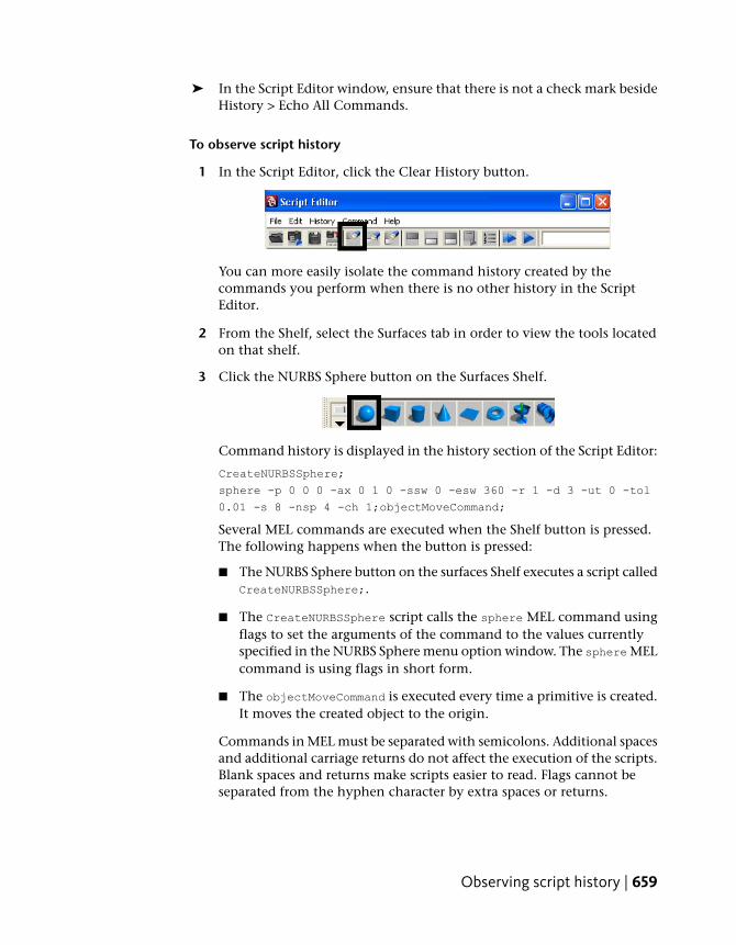
➤ In the Script Editor window, ensure that there is not a check mark besideHistory > Echo All Commands.
To observe script history
1 In the Script Editor, click the Clear History button.
You can more easily isolate the command history created by thecommands you perform when there is no other history in the ScriptEditor.
2 From the Shelf, select the Surfaces tab in order to view the tools locatedon that shelf.
3 Click the NURBS Sphere button on the Surfaces Shelf.
Command history is displayed in the history section of the Script Editor:
CreateNURBSSphere;
sphere -p 0 0 0 -ax 0 1 0 -ssw 0 -esw 360 -r 1 -d 3 -ut 0 -tol
0.01 -s 8 -nsp 4 -ch 1;objectMoveCommand;
Several MEL commands are executed when the Shelf button is pressed.The following happens when the button is pressed:
■ The NURBS Sphere button on the surfaces Shelf executes a script calledCreateNURBSSphere;.
■ The CreateNURBSSphere script calls the sphere MEL command usingflags to set the arguments of the command to the values currentlyspecified in the NURBS Sphere menu option window. The sphere MELcommand is using flags in short form.
■ The objectMoveCommand is executed every time a primitive is created.It moves the created object to the origin.
Commands in MEL must be separated with semicolons. Additional spacesand additional carriage returns do not affect the execution of the scripts.Blank spaces and returns make scripts easier to read. Flags cannot beseparated from the hyphen character by extra spaces or returns.
Observing script history | 659

TIP For more details on these flags, see sphere in the MEL Command Reference.
The MEL Command Reference gives a complete listing of the functionality of allMEL commands and flags.
NOTE You can copy commands from the Script Editor history section and pastethem in the input section to execute them.
➤ Delete the NURBS sphere by pressing the delete key on your keyboard.
To type a MEL command in the Script Editor
1 Select a MEL tab in the Script Editor.
Script Editor tabs allow you to quickly switch between MEL and Pythonscript entry modes. You can create additional Script Editor tabs to serveas a temporary holding area for scripts.
2 Type the following command in the input section of the Script Editor.
polyCube;
TIP When asked to type a command, you can copy it from these tutorialsand paste it into the Script Editor input section.
3 Execute the command by pressing Enter on the numeric part of yourkeyboard.
You must always type Enter on the numeric keypad or Ctrl+Enter (theregular Enter on your keyboard) to execute commands. Typing regularEnter just creates a new line in the Script Editor input.
A polygonal cube is created at the origin.
660 | Chapter 13 Scripting in Maya

The command is removed from the input section of the Script Editorafter execution. The command and the result of the command is outputto the history section of the Script Editor:
polyCube;
// Result: pCube1 polyCube1 //
NOTE In future lessons, when a series of MEL or Python commands createsoutput, only the output created by the commands will be referred to asoutput to the Script Editor.
Comments in MEL begin with // and anything which follows these characterson a line is ignored by MEL. The same convention is used for displaying resultsof commands and output in the Script Editor history section. Similarly, results,comments and messages output by Python are prefaced with the Pythoncommenting character ( # ).
NOTE In the rest of this lesson and the remaining MEL lessons, when asked totype a command, execute the command after typing it with the Enter on thenumeric keypad on your keyboard. You can also execute commands with Ctrl+Enter(Windows) or Ctrl+Return (Mac OS X).
TIP If you do not want the command to be removed from the input section ofthe Script Editor after execution, highlight the command before execution byselecting it with the mouse.
Modifying object attributesWhen you perform an action on an object in the Maya user interface, you areusing Maya commands to change the attributes of selected objects. You canuse the same Maya commands explicitly to edit the attributes of objects inthe scene.
To use the move command
1 With the polygonal cube selected, type the following in the Script Editor:
move 3 2 1;
Modifying object attributes | 661

The polygonal cube is moved to the XYZ co-ordinates 3,2,1.
The move command has set the translate attributes to the specifiedarguments of the command. These arguments are called commandarguments as they are not used with flags.
When a command is typed into the Script Editor, it acts on the currentselection, unless an object name is provided as an argument to thecommand.
2 With the polygonal cube selected, type the following in the Script Editor:
move -1 -2 -3 -relative;
The polygonal cube moved relative to its current position by -1,-2,-3 inXYZ.
The move command is used with the relative flag to change the methodin which the command executes. The relative flag does not have anyarguments; the values -1,-2,-3 are command arguments used with themove command. The values are prefaced by a negative sign, but are notrecognized as flags as they do not contain any of the flag keywords.
This is equivalent to using the Move tool in the Maya interface.
To specify attributes of geometry with flags
➤ Create a polygonal sphere with a radius of two and four subdivisions inX by typing the following in the Script Editor:
polySphere -radius 2 -subdivisionsX 4;
662 | Chapter 13 Scripting in Maya
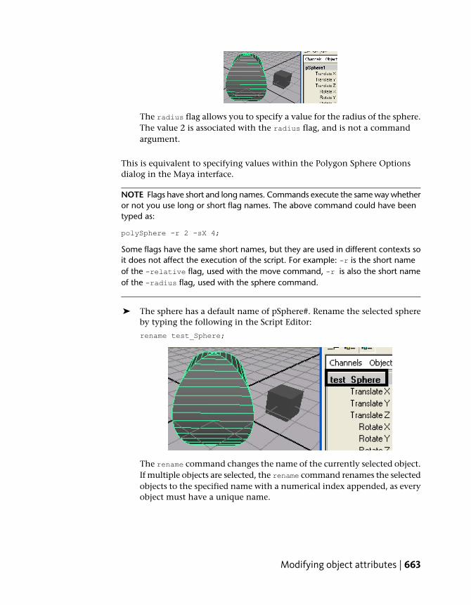
The radius flag allows you to specify a value for the radius of the sphere.The value 2 is associated with the radius flag, and is not a commandargument.
This is equivalent to specifying values within the Polygon Sphere Optionsdialog in the Maya interface.
NOTE Flags have short and long names. Commands execute the same way whetheror not you use long or short flag names. The above command could have beentyped as:
polySphere -r 2 -sX 4;
Some flags have the same short names, but they are used in different contexts soit does not affect the execution of the script. For example: -r is the short nameof the -relative flag, used with the move command, -r is also the short nameof the -radius flag, used with the sphere command.
➤ The sphere has a default name of pSphere#. Rename the selected sphereby typing the following in the Script Editor:
rename test_Sphere;
The rename command changes the name of the currently selected object.If multiple objects are selected, the rename command renames the selectedobjects to the specified name with a numerical index appended, as everyobject must have a unique name.
Modifying object attributes | 663
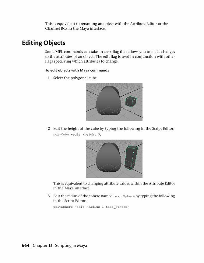
This is equivalent to renaming an object with the Attribute Editor or theChannel Box in the Maya interface.
Editing ObjectsSome MEL commands can take an edit flag that allows you to make changesto the attributes of an object. The edit flag is used in conjunction with otherflags specifying which attributes to change.
To edit objects with Maya commands
1 Select the polygonal cube
2 Edit the height of the cube by typing the following in the Script Editor:
polyCube -edit -height 3;
This is equivalent to changing attribute values within the Attribute Editorin the Maya interface.
3 Edit the radius of the sphere named test_Sphere by typing the followingin the Script Editor:
polySphere -edit -radius 1 test_Sphere;
664 | Chapter 13 Scripting in Maya
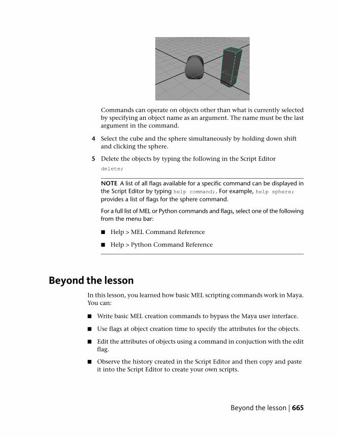
Commands can operate on objects other than what is currently selectedby specifying an object name as an argument. The name must be the lastargument in the command.
4 Select the cube and the sphere simultaneously by holding down shiftand clicking the sphere.
5 Delete the objects by typing the following in the Script Editor
delete;
NOTE A list of all flags available for a specific command can be displayed inthe Script Editor by typing help command;. For example, help sphere;
provides a list of flags for the sphere command.
For a full list of MEL or Python commands and flags, select one of the followingfrom the menu bar:
■ Help > MEL Command Reference
■ Help > Python Command Reference
Beyond the lessonIn this lesson, you learned how basic MEL scripting commands work in Maya.You can:
■ Write basic MEL creation commands to bypass the Maya user interface.
■ Use flags at object creation time to specify the attributes for the objects.
■ Edit the attributes of objects using a command in conjuction with the editflag.
■ Observe the history created in the Script Editor and then copy and pasteit into the Script Editor to create your own scripts.
Beyond the lesson | 665

Before proceeding with the next lesson you may want to review the materialpresented in this lesson so you are familiar with the concepts and skills. Somesuggested tasks you can try on your own include:
■ Practice using creation commands through the user interface and observingthe resulting Script Editor history.
■ Look through the MEL Command Reference to see more commoncommands.
■ Practice copying and pasting commands from the Script Editor historysection to the Script Editor input section.
Lesson 2: Saving scripts to the Shelf
Introduction
In this lesson, you set up a three-point lighting system using MEL and savethose MEL commands as a button on the Shelf. This lets you quickly set up athree-point lighting system in future scenes. You learn how to:
■ Enter MEL commands in place of selecting menu items
■ Create a shelf button to run a series of commands
Three-point lighting uses three different kinds of lights:
■ A main light to light the subject, cast shadows and produce highlights
■ A fill light to decrease the contrast caused by the main light
■ A rim light so the object stands out against the background
666 | Chapter 13 Scripting in Maya

Three-point lighting is used extensively in film, photography and computergraphics.
Setting up the sceneHere, you create some primitive objects to display lighting and shading .
1 Select File > New Scene to create a new scene.
2 Select Window > General Editors > Script Editor to open the Script Editor.
3 Create a ground plane by typing the following:
polyPlane -height 40 -width 40;
A plane appears at the origin.
The height and width flags specify the dimensions of the plane.
4 Create a NURBS torus by typing the following
torus -axis 0 1 0 -heightRatio 0.5;
A torus appears at the origin.
The axis of the torus specifies the orientation of the major axis of thetorus. The height ratio flag specifies the ratio of the major radius of thetorus to the height of the torus.
5 Reposition the torus so it is not intersecting the plane by typing thefollowing with the torus selected.
move 0 0.5 0;
The move command takes the argument (x, y, z), specifying how muchand in what direction to move the selected or named object. This abovecommand moves the torus 0.5 units up on the Y-axis.
6 Bring focus to the selected torus in the scene view by pressing f.
7 Render the scene by clicking the render button on the Status Line.
The Render View opens with a rendered image of the scene.
Setting up the scene | 667

8 Save the rendered image by clicking the Keep image button . Thislets you compare your rendered image with future rendered images.
A scroll bar at the bottom of the Render View lets you scroll through yoursaved rendered images.
In the next steps, you type commands to create three-point lighting in thescene and record them as script history for later use.
Recording the script historyIn order to make a shelf button, you need to create Script Editor history tocopy to the shelf. In this procedure, you create a three-point lighting systemfor the current geometry using MEL, copy the script history, and apply thecreated three-point lighting to an existing scene.
To create the main lighting
1 Clear Script Editor history by clicking the Clear History button .
2 Create a directional light for the main lighting by typing the following:
directionalLight -intensity 1;
668 | Chapter 13 Scripting in Maya

Certain commands require that you to refer to the light by name.
3 Rename the selected light to “main_light” by typing the following:
rename main_light;
4 Enable the main light to cast shadows by typing the following:
setAttr "main_lightShape.useDepthMapShadows" 1;
The setAttr command allows you to set attributes of a node. In the abovecommand, you are enabling depth map shadows on the main light.
5 Adjust the resolution of the shadow maps so that the shadows appearsharper by typing the following:
setAttr "main_lightShape.dmapResolution" 2048;
In the above command, you are increasing the resolution of the depthmap shadows to 2048.
6 Position and aim the main light by typing the following:
move 0 3 0;
rotate -30 0 0;
Next, you create a rim light for the scene to help differentiate the torus fromits background.
To create the rim light
1 Create a point light by typing the following:
pointLight -intensity 2 -rgb 0.9 0.9 1;
The intensity flag has been used to set the brightness of the light. The-rgb flag sets the color and takes three values: red, green and blue. Thered and green values are less than the blue value, so the light has a bluetint.
2 Rename the light by typing the following:
rename back_light;
3 Reposition the light behind the torus by typing the following:
move -relative -1.5 1 -1.5;
Next, you create a fill light for the scene to soften the main lighting, fill theshadowed part of the torus and decrease the overall contrast of the lightingin the scene.
Recording the script history | 669

To create the fill lighting
1 Create a point light with an intensity of 0.5 by typing the following:
pointLight -intensity 0.5;
2 Rename the light by typing the following:
rename fill_light;
3 Reposition the light above the torus in a way so that the light rays fromthe fill light are approximately 90 degrees to those of the main light bytyping the following:
move -relative 4 6 2;
Compare the rendered images
Rendering the image
1 Render the scene in the perspective view by selecting the render scene
button on the Status Line.
2 Save the rendered image by clicking the Keep Image button in theRender View.
3 Compare the two images using the scroll bar at the bottom of the window.
The newly rendered image has a shadow. If there was no fill light, detail wouldbe lost in the shadowed area, as the shadow would be black. The rim highlightsemphasize the curvature of the torus and help to differentiate the torus fromthe background.
670 | Chapter 13 Scripting in Maya

When creating three-point lighting in a scene with multiple objects, typicallythere is a main light that provides the main lighting for the scene, and eachobject in the scene has a linked fill and rim light.
Your three-point lighting script only works for objects of medium scale locatedat the origin, but once the lights are created, you can tweak them to bettersuit your scene.
Saving the history as a buttonYou can save Script Editor history as a Shelf button.
To create the shelf button
1 Highlight all the text in the history window by clicking at the beginningof the history in the upper section of the Script Editor and dragging theselection to the end of the Script Editor history section.
2 Release the mouse button. The selected text should read:
directionalLight -intensity 1; rename main_light; setAttr
"main_lightShape.useDepthMapShadows" 1; setAttr "main_light
Shape.dmapResolution" 1024; move 0 3 0; rotate -30 0 0; point
Light -intensity 2 -rgb .9 .9 1; rename back_light; move -r -1.5
1 -1.5; pointLight -intensity .5; rename fill_light; move -r 4
6 2;
3 Middle-drag the selected text to the shelf.
A pop-up window asks you which type of shelf button you are saving.
Saving the history as a button | 671
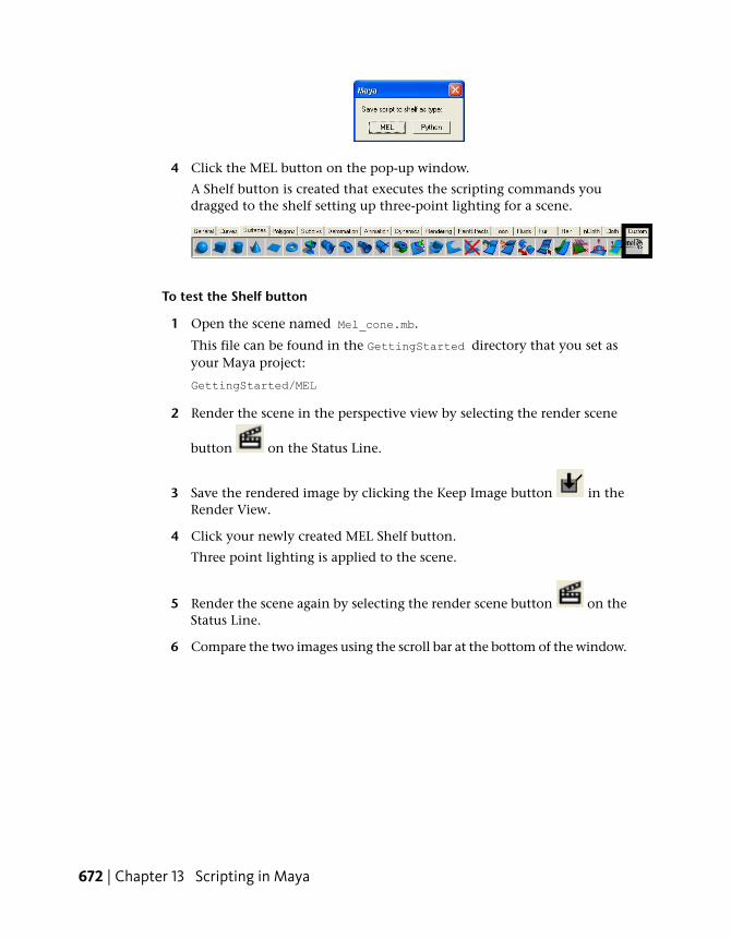
4 Click the MEL button on the pop-up window.
A Shelf button is created that executes the scripting commands youdragged to the shelf setting up three-point lighting for a scene.
To test the Shelf button
1 Open the scene named Mel_cone.mb.
This file can be found in the GettingStarted directory that you set asyour Maya project:
GettingStarted/MEL
2 Render the scene in the perspective view by selecting the render scene
button on the Status Line.
3 Save the rendered image by clicking the Keep Image button in theRender View.
4 Click your newly created MEL Shelf button.
Three point lighting is applied to the scene.
5 Render the scene again by selecting the render scene button on theStatus Line.
6 Compare the two images using the scroll bar at the bottom of the window.
672 | Chapter 13 Scripting in Maya

To delete the Shelf button
➤ Middle-drag the Shelf button you want deleted to the trash can icon onthe far right of the Shelf.
NOTE The pointer icon changes to a icon when you are dragging a Shelfbutton.
Beyond the LessonIn this lesson, you learned how to copy history from the Script Editor historysection to create Shelf buttons so that you can quickly execute a series ofcommands. You can:
■ Save multiple MEL script commands as a Shelf button.
■ Type basic MEL creation commands to bypass the Maya user interface.
■ Use additional MEL script commands and MEL script command flags.
Here are some other things you can do with Shelf buttons.
■ You can save the custom settings for a menu option box command as ashelf button by setting the parameters in the option box, and then selectingthe item from the menu while holding down Shift+Ctrl (Windows) orShift+Control+Option (Mac OS X).
■ You can add custom images to a shelf button, change the name of a shelfbutton, or change the commands associated with a shelf button by selectingWindow > Settings/Preferences > Shelf Editor. For more information, see
Beyond the Lesson | 673
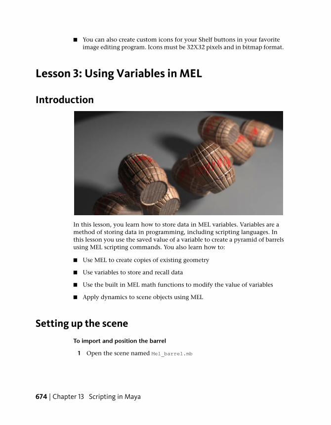
■ You can also create custom icons for your Shelf buttons in your favoriteimage editing program. Icons must be 32X32 pixels and in bitmap format.
Lesson 3: Using Variables in MEL
Introduction
In this lesson, you learn how to store data in MEL variables. Variables are amethod of storing data in programming, including scripting languages. Inthis lesson you use the saved value of a variable to create a pyramid of barrelsusing MEL scripting commands. You also learn how to:
■ Use MEL to create copies of existing geometry
■ Use variables to store and recall data
■ Use the built in MEL math functions to modify the value of variables
■ Apply dynamics to scene objects using MEL
Setting up the scene
To import and position the barrel
1 Open the scene named Mel_barrel.mb
674 | Chapter 13 Scripting in Maya

This file can be found in the GettingStarted\MEL directory that you setas your Maya project.
2 Open the Script Editor by selecting Window > General Editors > ScriptEditor.
3 Select the barrel with the select tool.
4 In the Script Editor, type the following:
Type exactly as below:
rotate -r 0 0 90;
The barrel is rotated 90 degrees about the Z axis.
Storing scene informationYou will store the value of the measurement annotation as a variable. A variableis a name used for convenience to refer to a certain location in memory. Thislocation in memory can store data.
Variables have four main characteristics; name, type, value and scope. Name,type and scope are defined at creation time. Defining the name and type ofa variable is referred to as declaring a variable. In MEL the name of the variableis always prefixed by the “$” symbol, indicating to the scripting language thatthe following characters name a variable.
The scope of the variable determines where the variable can be accessed from.If a variable is declared within a block of code, it cannot be accessed fromoutside the block of code.
Storing scene information | 675
Name and type cannot change after creation. The value of a variable canchange, but the value must be of the earlier defined type.
NOTE Variables in MEL should always have their type explicitly defined. If notexplicitly stated, the scripting language attempts to imply a data type for thevariable from the context of the first appearance of the variable. It is good practiceto explicitly declare variables as implicitly defining variables can lead to scriptingerrors and slows down the execution of the script.
To store scene information as a variable
1 In the Script Editor, type the following and press enter:
float $diameter_barrel;
This command declares a variable of data type float, with the namediameter_barrel. A floating point value is a number containing a decimal.
2 To assign a value to the variable, type the following.
$diameter_barrel = 4.2;
The diameter of the barrel is 4.2 units. This value from the scene isassigned to the variable. A value is assigned to a variable with theassignment operator (=).
Storing other types of data
MEL also supports other data types that are common to most otherprogramming languages.
To declare a string variable
➤ Type the following in the Script Editor
string $testString = "this is a test";
print $testString;
The following is output to the Script Editor:
this is a test
The string data type is used to store multiple characters. The printcommand outputs the value of a variable to the Script Editor.
NOTE Variables can be declared and assigned a value in the same statement.
676 | Chapter 13 Scripting in Maya

To declare an int variable
➤ Type the following in the Script Editor
int $testInt = 5;
print ($testInt/2);
The following is output to the Script Editor:
2
The int data type is used to store integer values. Integers are positive andnegative whole numbers. In programming, when an integer is dividedby another integer, the result is an integer, which is why the output hereis not 2.5 (2.5 is not an integer).
The print command’s argument is enclosed in brackets. The printcommand can only take one argument, so brackets are used to tell Mayato evaluate the contents of the brackets before executing the command.Brackets can also be nested in a method similar to mathematicalstatements to determine the order of evaluation of statements.
In the steps that follow, you create a row of barrels by spacing the barrelsevenly. This creates barrels that are just touching, which ensures that thereare no intersections during the rigid body simulation
In the next section, we’ll use the move command to position the duplicatebarrels, using the saved value of the diameter as an argument for the Z valueof the command.
Create a row of barrelsHere, we’ll use the stored value of the diameter to space the duplicates of thebarrel. Variable values can be recalled at any time. Variables can be used asvalues for arguments.
To duplicate the barrels
1 Select the barrel.
2 Duplicate the barrel by typing the following:
duplicate;
You have a duplicate of the first barrel, and it is the currently selectedobject.
3 Align the duplicate barrel with the original by moving the duplicate inZ by a value equal to its diameter by typing the following:
Create a row of barrels | 677
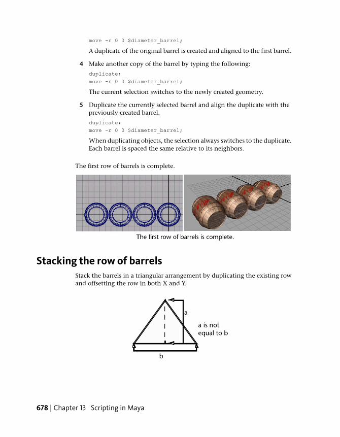
move -r 0 0 $diameter_barrel;
A duplicate of the original barrel is created and aligned to the first barrel.
4 Make another copy of the barrel by typing the following:
duplicate;
move -r 0 0 $diameter_barrel;
The current selection switches to the newly created geometry.
5 Duplicate the currently selected barrel and align the duplicate with thepreviously created barrel.
duplicate;
move -r 0 0 $diameter_barrel;
When duplicating objects, the selection always switches to the duplicate.Each barrel is spaced the same relative to its neighbors.
The first row of barrels is complete.
Stacking the row of barrelsStack the barrels in a triangular arrangement by duplicating the existing rowand offsetting the row in both X and Y.
678 | Chapter 13 Scripting in Maya

Using basic trigonometry, you can calculate the unknown height offset. MELhas a library of built-in functions that include trigonometry functions, tohandle these calculations.
NOTE Trigonometry functions are ratios that relate two sides of a right angledtriangle dependant on one of the angles of the triangle. Trigonometry functionsare often used for animation, as trigonometric functions are periodic. Periodicfunctions cycle their output values after a certain period. These functions can easilycreate cyclical or repeating animation.
Using MEL built-in functions to calculate the Y offsetSine is the ratio obtained by dividing the side opposite the angle by thehypotenuse. Since the center points of the barrels are spaced along the pointsof an equilateral triangle, all angles of the triangle are equal to 60°. If youmultiply the sine of 60° by the length of one of the sides of the triangle, theresult is the height of the triangle.
It is important to know which units of measurement the built-in functionsof a programming language use. Many programming languages, includingMEL and Python, perform trigonometric operations in radians. You mustconvert from degrees to radians when using the sine function to calculate theY offset.
NOTE Radians are a method of measuring sections of a circle. There are 360degrees in a circle, which is equivalent to 2pi radians.
To calculate the offset in Y
1 Declare a new variable to store the value of the Y offset by typing thefollowing:
Using MEL built-in functions to calculate the Y offset | 679

float $Y_offset;
2 Calculate the value of the Y-offset using the sine ratio. You must convertthe value of the angle to degrees with the degree to radian conversionfunction.
$Y_offset = $diameter_barrel * (sin(deg_to_rad(60)));
The assignment operator evaluates the right hand side of the expressionand assigns it to the left hand side. The degree to radian conversionfunction is the first to be evaluated, as it is within the most interior setof brackets. The sine function calculates the sine of the angle given inradians. The sine value is multiplied by the diameter to calculate the Yoffset. The variable is assigned the calculated value.
NOTE The variable $diameter_barrel does not change in value. Only thevariable on the left side of an assignment operator changes in value.
To stack the rows of barrels
1 Select and duplicate all the objects in the scene, by typing the following:
select -allDagObjects;
duplicate;
Using the select command with the -allDagObjects flag selects all DAG(Directed Acyclic Graph) objects, which are a set of objects that exist inthe scene such as geometry, IK chains and measure tools. Textures andanimation information do not belong to the Directed Acyclic Graph.
2 Offset the barrels by the radius of a barrel in X and the calculated$Y_offset in Y, divide the diameter by 2 to get the value of the radius.When duplicating the rows, you have created too many barrels.
move -r 0 $Y_offset ($diameter_barrel/2.0);
duplicate;
move -r 0 $Y_offset ($diameter_barrel/2.0);
duplicate;
move -r 0 $Y_offset ($diameter_barrel/2.0);
3 Using the Lasso tool, select the extra barrels.
4 Delete the extra barrels to obtain a pyramid shape.
680 | Chapter 13 Scripting in Maya

Creating dynamics with MEL commandsMaya lets you easily add dynamic properties to the objects in your scenes. Allattributes that can be modified by selecting menu items, can be accessed bysetting the arguments of a Maya command.
In this section you create a dynamic simulation using MEL so that the stackof barrels reacts to gravity and moves in a realistic manner. Apply a rigidBodynode to all of the barrels, add a gravity field and a passive rigid body planefor the barrels to collide with.
For more information about rigid bodies and fields within dynamics in Maya,see Lesson 2: Rigid bodies and constraints on page 554 and the Dynamics guidein the Maya Help.
To add rigid body nodes to the barrels using MEL
1 Select all the barrels by typing the following:
select -allDagObjects;
Creating dynamics with MEL commands | 681
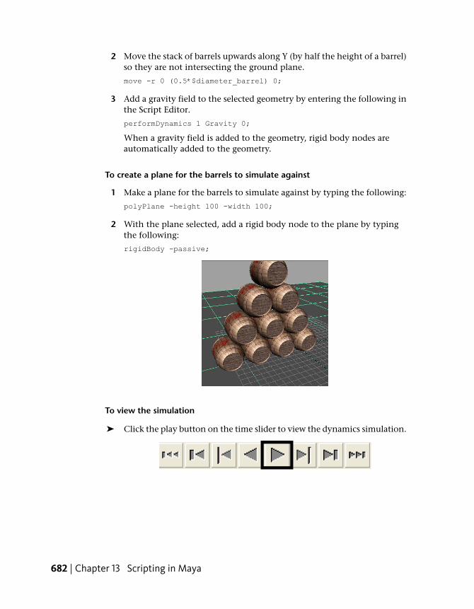
2 Move the stack of barrels upwards along Y (by half the height of a barrel)so they are not intersecting the ground plane.
move -r 0 (0.5*$diameter_barrel) 0;
3 Add a gravity field to the selected geometry by entering the following inthe Script Editor.
performDynamics 1 Gravity 0;
When a gravity field is added to the geometry, rigid body nodes areautomatically added to the geometry.
To create a plane for the barrels to simulate against
1 Make a plane for the barrels to simulate against by typing the following:
polyPlane -height 100 -width 100;
2 With the plane selected, add a rigid body node to the plane by typingthe following:
rigidBody -passive;
To view the simulation
➤ Click the play button on the time slider to view the dynamics simulation.
682 | Chapter 13 Scripting in Maya
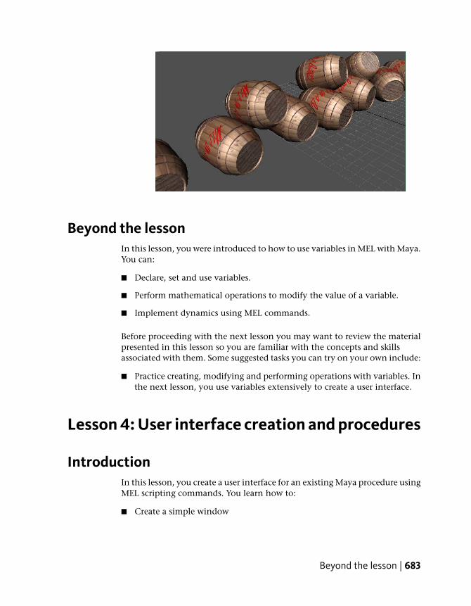
Beyond the lessonIn this lesson, you were introduced to how to use variables in MEL with Maya.You can:
■ Declare, set and use variables.
■ Perform mathematical operations to modify the value of a variable.
■ Implement dynamics using MEL commands.
Before proceeding with the next lesson you may want to review the materialpresented in this lesson so you are familiar with the concepts and skillsassociated with them. Some suggested tasks you can try on your own include:
■ Practice creating, modifying and performing operations with variables. Inthe next lesson, you use variables extensively to create a user interface.
Lesson 4: User interface creation and procedures
IntroductionIn this lesson, you create a user interface for an existing Maya procedure usingMEL scripting commands. You learn how to:
■ Create a simple window
Beyond the lesson | 683

■ Use conditional statements to check the existence of a window
■ Use a built-in Maya procedure
■ Link a procedure to a user interface
Creating a windowThe first step in creating custom user interfaces is to create a window. Thiswindow contains the elements of the user interface such as text, buttons andother controls.
To create a window
1 Type the following commands into a MEL tab of the Script Editor.
window -resizeToFitChildren 1; showWindow;
A window appears.
The -resizeToFitChildren flag on the window command specifies thatthe window automatically resizes to fit all of the elements within thewindow. This flag must have a value: a value of 1 turns on the flag, avalue of 0 turns it off.
When you create a window, it is not visible until you use the showWindowcommand. The showWindow command without any arguments makes thelast window created visible.
2 Close the window clicking the X in the upper right hand corner.
Referencing controls
When creating windows with MEL scripting, you must ensure that everywindow and user interface control is given a unique name. If you do notexplicitly give a window a name, it gets a default name. (In the previousprocedure, the name of the window was window1, even though you didn’t
684 | Chapter 13 Scripting in Maya

use it.) You cannot reference or modify windows or controls that you don’tknow the name of.
To refer to a user interface element by name
1 Create a window with text and a button that closes it by typing thefollowing in a MEL tab of the Script Editor:
window -resizeToFitChildren 1 testwindow; columnLayout; text
-label "This is a test window you can close by\ clicking the
button below."; button -label "Close" -command "deleteUI
testwindow"; showWindow;
2 Press the Close button in the window.
The window closes.
Discussion: creating a simple window
In your window, you created elements for your user interface, called controls.All user interface controls must be created within a layout. Layouts instructMaya how to arrange the user interface elements in the window.
There are many different types of layouts—for example, formLayout androwLayout—but the simplest and easiest to use is the columnLayout. ThecolumnLayout lays out your controls in a column, one underneath the other.For more information on layouts, see Layouts of the MEL and Expressionsguide.
Within the layout you created a text control, with the text command. Thelabel flag’s argument is the text displayed in the window.
The button is created by the button command. The argument of the commandflag is a MEL command that is executed when the button is pressed. In thiscase, pressing the button executes the deleteUI command, which deletes thewindow you just created.
Scripts spanning multiple lines
In this script, individual commands span multiple lines. Commands can spanmultiple lines as long as the end line character is at the end of the command.One convention in MEL is to have the command keyword on one line, andpair the modifier flags and values on separate lines underneath the command,as in this example.
Creating a window | 685

Strings can’t be split up over multiple lines without the use of a specialcharacter. To split a string over multiple lines, use the back slash (\) character.For example:
print "With the \\ character, you can \ split a string over \
multiple lines.";
To have a backslash appear in a string, you must use a double backslash. Thebackslash character is an escape character. Escape characters tell the scriptinterpreter that the character that follows is literal. Certain special symbolscan be created using the escape character in combination with other characters.For example, to display quotes within a string:
print "Jim said \"Hello!\" to the Maya user";
Window namingAs user interface scripts get more complex, it is possible that you may makea syntax error. If a user interface script partially executes and halts on an error,the window still exists, but the window is not visible. If you fix the problemand would like to execute the script again, you must either give the windowa new name, or delete the hidden window.
Resolving naming conflicts
In the next section, you use conditional statements to resolve window namingconflicts. Conditional statements allow a section of code to execute dependingon the value of a variable or the state of an object in the scene.
To resolve conflicting window names
1 Create a window with a scripting error inserted before the showWindowcommand by typing the following in a MEL tab of the Script Editor:
window testwindow; fake_command; showWindow;
An error is output to the Script Editor.
// Error: line 2: Cannot find procedure "fake_command;". //
The window is not displayed, but still exists.
2 Create another window with the same name by typing the following ina MEL tab of the Script Editor:
window testwindow; showWindow;
An error is output to the Script Editor.
686 | Chapter 13 Scripting in Maya
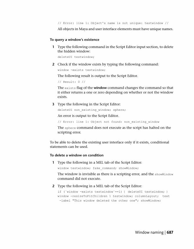
// Error: line 1: Object's name is not unique: testwindow //
All objects in Maya and user interface elements must have unique names.
To query a window’s existence
1 Type the following command in the Script Editor input section, to deletethe hidden window:
deleteUI testwindow;
2 Check if the window exists by typing the following command:
window -exists testwindow;
The following result is output to the Script Editor.
// Result: 0 //
The exists flag of the window command changes the command so thatit either returns a one or zero depending on whether or not the windowexists.
3 Type the following in the Script Editor:
deleteUI non_existing_window; sphere;
An error is output to the Script Editor.
// Error: line 1: Object not found: non_existing_window
The sphere command does not execute as the script has halted on thescripting error.
To be able to delete the existing user interface only if it exists, conditionalstatements can be used.
To delete a window on condition
1 Type the following in a MEL tab of the Script Editor:
window testwindow; fake_command; showWindow;
The window is invisible as there is a scripting error, and the showWindowcommand did not execute.
2 Type the following in a MEL tab of the Script Editor:
if (`window -exists testwindow`==1) { deleteUI testwindow; }
window -resizeToFitChildren 1 testwindow; columnLayout; text
-label "This window deleted the other one"; showWindow;
Window naming | 687
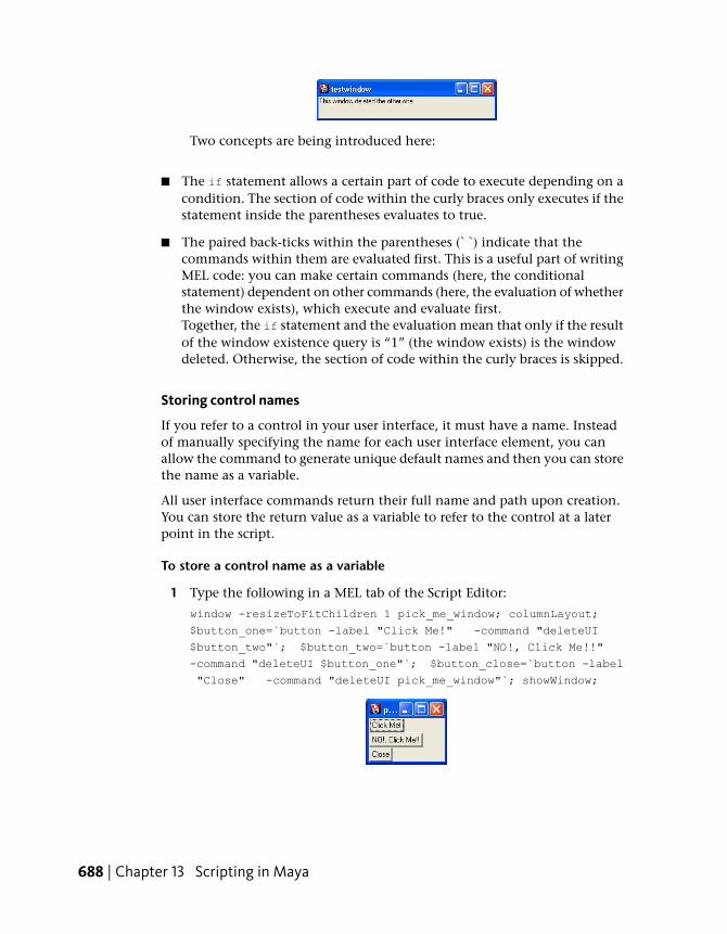
Two concepts are being introduced here:
■ The if statement allows a certain part of code to execute depending on acondition. The section of code within the curly braces only executes if thestatement inside the parentheses evaluates to true.
■ The paired back-ticks within the parentheses (` `) indicate that thecommands within them are evaluated first. This is a useful part of writingMEL code: you can make certain commands (here, the conditionalstatement) dependent on other commands (here, the evaluation of whetherthe window exists), which execute and evaluate first.Together, the if statement and the evaluation mean that only if the resultof the window existence query is “1” (the window exists) is the windowdeleted. Otherwise, the section of code within the curly braces is skipped.
Storing control names
If you refer to a control in your user interface, it must have a name. Insteadof manually specifying the name for each user interface element, you canallow the command to generate unique default names and then you can storethe name as a variable.
All user interface commands return their full name and path upon creation.You can store the return value as a variable to refer to the control at a laterpoint in the script.
To store a control name as a variable
1 Type the following in a MEL tab of the Script Editor:
window -resizeToFitChildren 1 pick_me_window; columnLayout;
$button_one=`button -label "Click Me!" -command "deleteUI
$button_two"`; $button_two=`button -label "NO!, Click Me!!"
-command "deleteUI $button_one"`; $button_close=`button -label
"Close" -command "deleteUI pick_me_window"`; showWindow;
688 | Chapter 13 Scripting in Maya
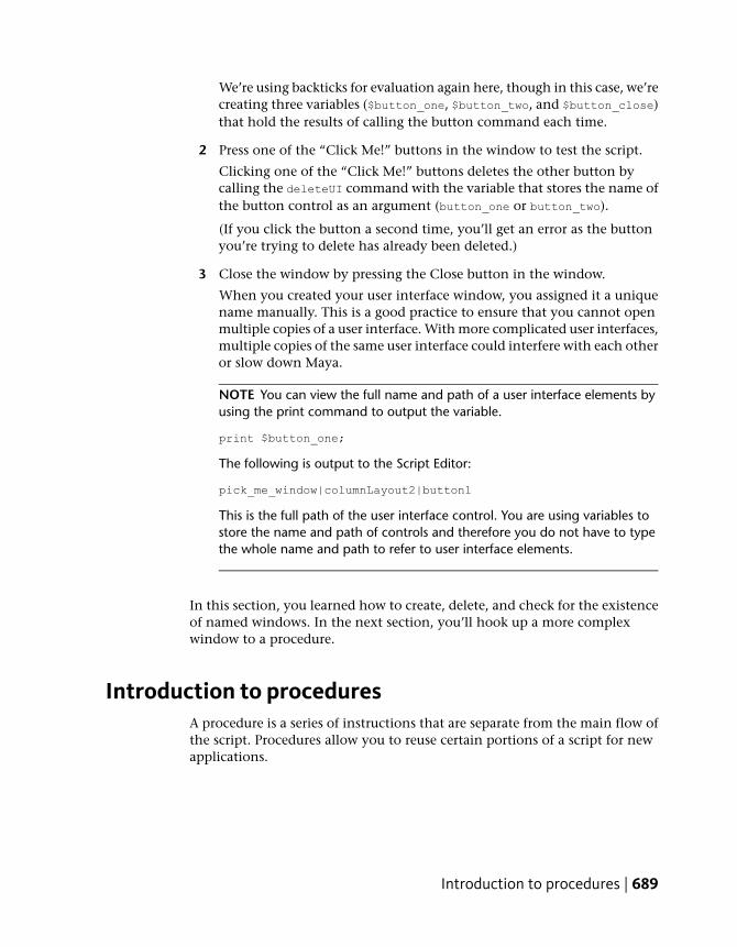
We’re using backticks for evaluation again here, though in this case, we’recreating three variables ($button_one, $button_two, and $button_close)that hold the results of calling the button command each time.
2 Press one of the “Click Me!” buttons in the window to test the script.
Clicking one of the “Click Me!” buttons deletes the other button bycalling the deleteUI command with the variable that stores the name ofthe button control as an argument (button_one or button_two).
(If you click the button a second time, you’ll get an error as the buttonyou’re trying to delete has already been deleted.)
3 Close the window by pressing the Close button in the window.
When you created your user interface window, you assigned it a uniquename manually. This is a good practice to ensure that you cannot openmultiple copies of a user interface. With more complicated user interfaces,multiple copies of the same user interface could interfere with each otheror slow down Maya.
NOTE You can view the full name and path of a user interface elements byusing the print command to output the variable.
print $button_one;
The following is output to the Script Editor:
pick_me_window|columnLayout2|button1
This is the full path of the user interface control. You are using variables tostore the name and path of controls and therefore you do not have to typethe whole name and path to refer to user interface elements.
In this section, you learned how to create, delete, and check for the existenceof named windows. In the next section, you’ll hook up a more complexwindow to a procedure.
Introduction to proceduresA procedure is a series of instructions that are separate from the main flow ofthe script. Procedures allow you to reuse certain portions of a script for newapplications.
Introduction to procedures | 689

In this section, you use a procedure that is included with Maya (makeroll,which simulates an object rolling on a plane). Later in the lesson, you linkthis procedure to a user interface to provide an easier way to use the procedure.
To execute the makeRoll procedure
1 Create a cube and a ground plane by typing the following in a MEL tabof the Script Editor:
polyCube -name roll_Cube; polyPlane -height 10 -width 10;
2 Execute the makeRoll procedure by typing the following in a MEL tab ofthe Script Editor:
makeRoll roll_Cube 0 1 1.0;
The makeRoll procedure requires the following arguments: the name ofthe object to act on, the height of the ground plane, the type ofsimulation, and the diameter of the object. The type of simulation iseither box or sphere simulation. Rolling simulation is determined usinga bounding sphere when simulation type is set to 0, or a bounding boxwhen simulation type is set to 1.
3 Set the current frame to two by selecting the current frame box and typinga two.
The expressions set up by the makeRoll procedure only take effect whenthe frame is greater than one.
4 Select the cube with the Move tool.
5 Move the cube along the plane in X and Z using the Move tool.
The cube rolls on the ground plane.
690 | Chapter 13 Scripting in Maya

You have successfully loaded and used the makeRoll procedure. Now, you’lllink the procedure to a user interface.
Loading a script fileYou can read and edit script files other people have created in the Script Editor.In this section, you open a script that contains a completed user interface forthe makeRoll procedure. However, the user interface is only a layout, and doesnot contain any functionality.
To prepare to open the script
1 In the Script Editor, ensure that Command > Show Line Numbers ischecked.
When Show Line Numbers is on, line numbers appear beside thecommands in the Script Editor. The lesson occasionally refers to linenumbers to tell you where to make a modification to the script. Whenline numbers are referred to in the lesson, they are always the linenumbers of the original script.
2 Create a new tab in the Script Editor by selecting Command > New Tab.
A pop-up window asks you in which language should the commandsentered in this tab execute in.
3 Click the MEL button on the pop-up window.
You created a second MEL tab in the Script Editor.
4 Select Command > Rename Tab.
5 Enter MEL2.
The tab is renamed.
Loading a script file | 691
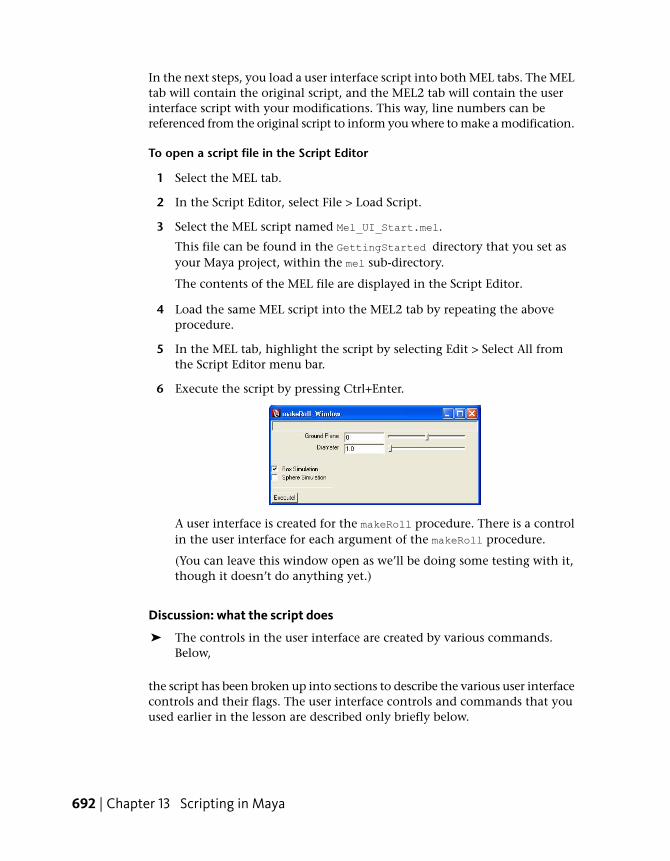
In the next steps, you load a user interface script into both MEL tabs. The MELtab will contain the original script, and the MEL2 tab will contain the userinterface script with your modifications. This way, line numbers can bereferenced from the original script to inform you where to make a modification.
To open a script file in the Script Editor
1 Select the MEL tab.
2 In the Script Editor, select File > Load Script.
3 Select the MEL script named Mel_UI_Start.mel.
This file can be found in the GettingStarted directory that you set asyour Maya project, within the mel sub-directory.
The contents of the MEL file are displayed in the Script Editor.
4 Load the same MEL script into the MEL2 tab by repeating the aboveprocedure.
5 In the MEL tab, highlight the script by selecting Edit > Select All fromthe Script Editor menu bar.
6 Execute the script by pressing Ctrl+Enter.
A user interface is created for the makeRoll procedure. There is a controlin the user interface for each argument of the makeRoll procedure.
(You can leave this window open as we’ll be doing some testing with it,though it doesn’t do anything yet.)
Discussion: what the script does
➤ The controls in the user interface are created by various commands.Below,
the script has been broken up into sections to describe the various user interfacecontrols and their flags. The user interface controls and commands that youused earlier in the lesson are described only briefly below.
692 | Chapter 13 Scripting in Maya

Conditional statement
if(`window -exists makeRoll_Window`==1) { deleteUI makeRoll_Win
dow; }
The conditional statement checks if a window with the specified name exists.If the window exists, it deletes it.
Window command
window -resizeToFitChildren 1 makeRoll_Window;
The window command creates a user interface window to contain the controls.For more information, see Creating a window on page 684.
Column layout
columnLayout;
The columnLayout command creates a layout that arranges the controls withinit in a column. For more information, see Referencing controls on page 684.
Text field commands
$obj_name_text = `textField -editable 0 -width 400 -text
name_Of_Object`;
The command textField creates an editable text field. The text field commandhas multiple flags. The name and path of the text field are stored as a variable.See Storing control names on page 688.
■ The editable flag enables or disables editing of the text field.
■ The width flag sets the width of the control.
■ The text flag sets the contents of the text field.
Slider commands
$ground_int= `intSliderGrp -minValue -20 -maxValue 20 -value 0
-fieldMinValue -20 -fieldMaxValue 20 -field 1 -label "Ground
Plane"`; $diameter_float= `floatSliderGrp -value 1.0 -minValue
1.0 -fieldMinValue 1.0 -field 1 -label "Diameter"`;
The commands intSliderGrp and floatSliderGrp create sliders. Commandsending in Grp create a group of linked controls. The slider commands createcontrols for a label, a value box and a slider. The slider command has multiple
Loading a script file | 693
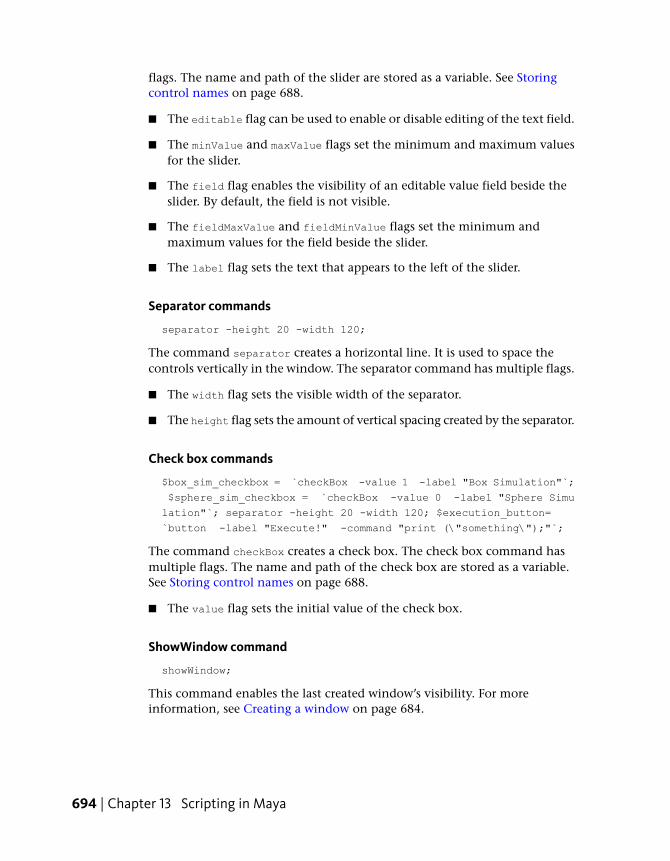
flags. The name and path of the slider are stored as a variable. See Storingcontrol names on page 688.
■ The editable flag can be used to enable or disable editing of the text field.
■ The minValue and maxValue flags set the minimum and maximum valuesfor the slider.
■ The field flag enables the visibility of an editable value field beside theslider. By default, the field is not visible.
■ The fieldMaxValue and fieldMinValue flags set the minimum andmaximum values for the field beside the slider.
■ The label flag sets the text that appears to the left of the slider.
Separator commands
separator -height 20 -width 120;
The command separator creates a horizontal line. It is used to space thecontrols vertically in the window. The separator command has multiple flags.
■ The width flag sets the visible width of the separator.
■ The height flag sets the amount of vertical spacing created by the separator.
Check box commands
$box_sim_checkbox = `checkBox -value 1 -label "Box Simulation"`;
$sphere_sim_checkbox = `checkBox -value 0 -label "Sphere Simu
lation"`; separator -height 20 -width 120; $execution_button=
`button -label "Execute!" -command "print (\"something\");"`;
The command checkBox creates a check box. The check box command hasmultiple flags. The name and path of the check box are stored as a variable.See Storing control names on page 688.
■ The value flag sets the initial value of the check box.
ShowWindow command
showWindow;
This command enables the last created window’s visibility. For moreinformation, see Creating a window on page 684.
694 | Chapter 13 Scripting in Maya

NOTE In the script above, you do not explicitly declare your variables. This isbecause the return type of user interface creation commands is known to be astring, and cannot be any other data type. Later in the lesson, you will allow adata type to be implied, as you do not know what data type the return will be.
Linking the user interfaceCurrently the user interface in the window doesn’t do anything: moving thesliders and clicking the check boxes has no effect. In this section you learnhow to link the user interface to the makeRoll procedure you used earlier:
■ The textField in the user interface will display the currently selectedobject.
■ The check boxes in the window will be linked so that only one check boxcan be selected at once.
■ The button will execute the makeRoll procedure with the argumentsspecified in the window.
In the following steps you modify the user interface script.
A completed version of the user interface script named Mel_UI_Final.mel isavailable in the GettingStarted project directory, within the mel sub-directory.
Displaying the currently selected object
The makeRoll procedure does not act upon the currently selected object. Youwill modify the script so that the textField control will display the name ofthe currently selected object.
To return the name of the currently selected object, use the ls command (list)with the selection. Since you can select multiple objects in Maya, the returnfrom the ls command is not a string, it is a string array, even if only oneobject is selected. An array is an ordered list of values used to store multipleitems of the same data type within one variable. The makeRoll procedurecannot accept a string array as an argument, so you must modify the datareturned by ls -selection.
NOTE For more information on the ls command, see ls in the MEL CommandReference.
For more information on arrays, see Arrays in the MEL and Expressions guide.
Linking the user interface | 695
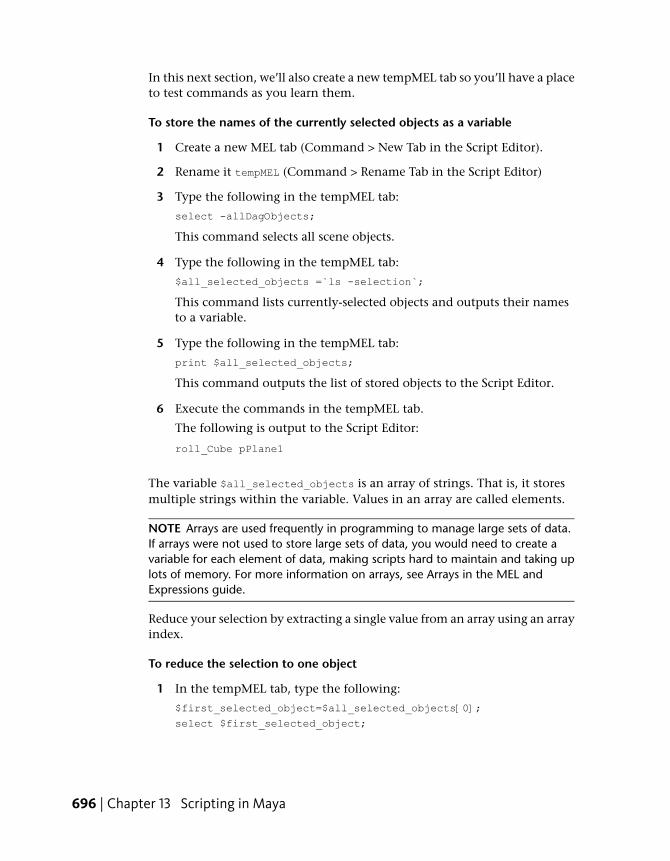
In this next section, we’ll also create a new tempMEL tab so you’ll have a placeto test commands as you learn them.
To store the names of the currently selected objects as a variable
1 Create a new MEL tab (Command > New Tab in the Script Editor).
2 Rename it tempMEL (Command > Rename Tab in the Script Editor)
3 Type the following in the tempMEL tab:
select -allDagObjects;
This command selects all scene objects.
4 Type the following in the tempMEL tab:
$all_selected_objects =`ls -selection`;
This command lists currently-selected objects and outputs their namesto a variable.
5 Type the following in the tempMEL tab:
print $all_selected_objects;
This command outputs the list of stored objects to the Script Editor.
6 Execute the commands in the tempMEL tab.
The following is output to the Script Editor:
roll_Cube pPlane1
The variable $all_selected_objects is an array of strings. That is, it storesmultiple strings within the variable. Values in an array are called elements.
NOTE Arrays are used frequently in programming to manage large sets of data.If arrays were not used to store large sets of data, you would need to create avariable for each element of data, making scripts hard to maintain and taking uplots of memory. For more information on arrays, see Arrays in the MEL andExpressions guide.
Reduce your selection by extracting a single value from an array using an arrayindex.
To reduce the selection to one object
1 In the tempMEL tab, type the following:
$first_selected_object=$all_selected_objects[0];
select $first_selected_object;
696 | Chapter 13 Scripting in Maya

The first element of the array, the roll_Cube, is selected.
Elements of an array are accessed using square brackets containing theindex number of the element you want to extract from the array. Theindex number of arrays start counting from zero.
2 Add the following commands to the top of your user interface script inthe MEL2 tab:
$all_selected_objects=`ls -selection`;
$first_selected_object=$all_selected_objects[0];
select $first_selected_object;
These commands change your selection to the object you selected first.
3 In the MEL2 tab, change the argument of the text flag located on line14 of the original script (you can use the MEL tab for reference) fromname_of_object to the following:
$first_selected_object
The command now reads:
$obj_name_text = `textField -editable 0 -width 400 -text
$first_selected_object`;
The text field now displays the currently selected object.
If you attempt to execute the modified user interface creation scriptwithout an object selected, an error occurs, as no elements exist in thestring array $all_selected_objects.
TIP Don’t execute the script from the MEL2 tab yet, as it will clear the taband we want to continue modifying the script. If you do want to execute thescript at any interim time, create a new MEL tab, copy the script into it, andexecute that.
Linking the check boxes
Check boxes can also use command flags, similar to a button. A check boxhas more functionality than a button, so the command flags are different.Check boxes have three possible command flags; changeCommand, onCommand,and offCommand:
■ The changeCommand flag triggers whenever the state of the check boxchanges.
■ The onCommand flag triggers when the check box is checked.
Linking the user interface | 697
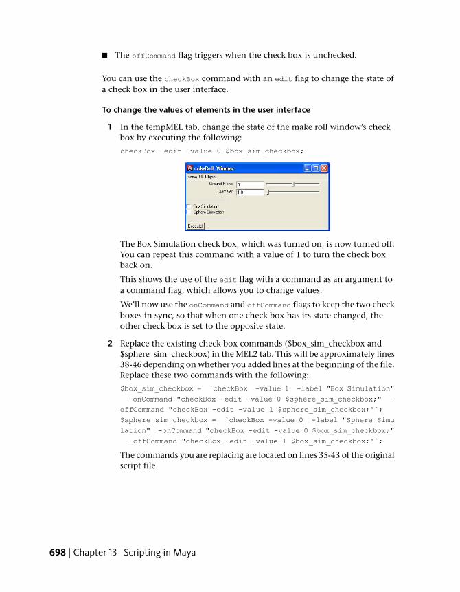
■ The offCommand flag triggers when the check box is unchecked.
You can use the checkBox command with an edit flag to change the state ofa check box in the user interface.
To change the values of elements in the user interface
1 In the tempMEL tab, change the state of the make roll window’s checkbox by executing the following:
checkBox -edit -value 0 $box_sim_checkbox;
The Box Simulation check box, which was turned on, is now turned off.You can repeat this command with a value of 1 to turn the check boxback on.
This shows the use of the edit flag with a command as an argument toa command flag, which allows you to change values.
We’ll now use the onCommand and offCommand flags to keep the two checkboxes in sync, so that when one check box has its state changed, theother check box is set to the opposite state.
2 Replace the existing check box commands ($box_sim_checkbox and$sphere_sim_checkbox) in the MEL2 tab. This will be approximately lines38-46 depending on whether you added lines at the beginning of the file.Replace these two commands with the following:
$box_sim_checkbox = `checkBox -value 1 -label "Box Simulation"
-onCommand "checkBox -edit -value 0 $sphere_sim_checkbox;" -
offCommand "checkBox -edit -value 1 $sphere_sim_checkbox;"`;
$sphere_sim_checkbox = `checkBox -value 0 -label "Sphere Simu
lation" -onCommand "checkBox -edit -value 0 $box_sim_checkbox;"
-offCommand "checkBox -edit -value 1 $box_sim_checkbox;"`;
The commands you are replacing are located on lines 35-43 of the originalscript file.
698 | Chapter 13 Scripting in Maya

Executing the procedure
The makeRoll procedure requires arguments to execute. To link it to thewindow, you must get the values for the arguments from the controls in theuser interface, and execute the makeRoll procedure with these arguments.
To get the values of the controls, you must use the query flag. The query flagallows commands to return values of attributes in the scene.
To query a value in the user interface
1 Change the value of the diameter slider to 10.01 by dragging the sliderto the right, or by typing a value in the diameter slider’s text field.
2 Print the value of the diameter slider by typing the following in thetempMEL tab:
print ("The diameter is: " + `floatSliderGrp -query -value
$diameter_float`);
The following is output to the Script Editor
The diameter is: 10.01
The query flag allows you to output a value to the Script Editor.
Change the command flag of the button so that it calls makeRoll commandwith arguments values that are the same as the specified values in the userinterface.
To link the button to the makeRoll procedure
➤ Replace the command flag of the execution button block in the MEL2tab (approximately line 57) with the following:
-command "makeRoll \ `textField -query -text $obj_name_text` \
`intSliderGrp -query -value $ground_int` \ `checkBox -query -
value $box_sim_checkbox` \ `floatSliderGrp -query -value $diamet
er_float`;"`;
Linking the user interface | 699

Every argument of the user interface is defined by querying the userinterface elements. The backslash at the end of a line allows the commandflag argument to span multiple lines.
Your user interface is now fully functional!
A completed version of the user interface script named Mel_UI_Final.mel isavailable in the GettingStarted project directory (GettingStarted/mel).
Saving the scriptTo use your script in other scenes, you must save it. To execute the MELcommands in a script file without having to open it every time you want touse it, you must use global procedures.
Once you’ve saved a MEL script file that contains a global procedure in thedefault script folder of Maya, you can access it whenever you type MELcommands. Other procedures in the script file can only be called by the globalprocedure(s) defined in the script file or other local procedures.
Maya automatically sources procedures in its default scripts folders at startup. A script in the default Maya script folder has the same name as a globalprocedure defined in the script file, when you type the name of the script file,the global procedure within the script file will be executed. This allows youto create scripts that operate similar to built-in Maya commands.
1 Type the following at the top of MEL2:
global proc makeRoll_create_UI() {
2 At the bottom of MEL2, type the following:
}
Your entire user interface script should be between the curly braces.
3 Highlight the entire script by selecting Edit > Select All from the ScriptEditor menu bar.
4 With the script highlighted, save the script by selecting File > Save Scriptfrom the Script Editor.
The Script Editor only saves the highlighted commands when saving ascript.
5 Save the script as makeRoll_create_UI.mel in the GettingStarted/melfolder.
700 | Chapter 13 Scripting in Maya
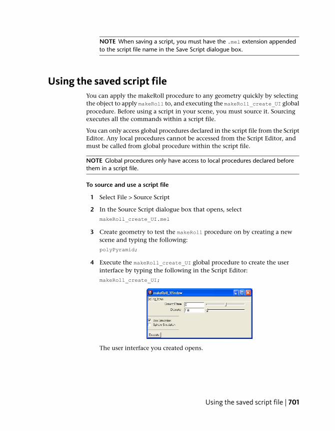
NOTE When saving a script, you must have the .mel extension appendedto the script file name in the Save Script dialogue box.
Using the saved script fileYou can apply the makeRoll procedure to any geometry quickly by selectingthe object to apply makeRoll to, and executing the makeRoll_create_UI globalprocedure. Before using a script in your scene, you must source it. Sourcingexecutes all the commands within a script file.
You can only access global procedures declared in the script file from the ScriptEditor. Any local procedures cannot be accessed from the Script Editor, andmust be called from global procedure within the script file.
NOTE Global procedures only have access to local procedures declared beforethem in a script file.
To source and use a script file
1 Select File > Source Script
2 In the Source Script dialogue box that opens, select
makeRoll_create_UI.mel
3 Create geometry to test the makeRoll procedure on by creating a newscene and typing the following:
polyPyramid;
4 Execute the makeRoll_create_UI global procedure to create the userinterface by typing the following in the Script Editor:
makeRoll_create_UI;
The user interface you created opens.
Using the saved script file | 701

5 Set the frame to greater than one to view the effects of the makeRollprocedure.
6 Set the following values in the makeRoll user interface:
■ Ground Plane = 0
■ Diameter = 1.0
■ Box Simulation = checked
■ Sphere Simulation = unchecked
7 Click the “Execute” button to setup the makeRoll expressions.
8 Move the pyramid in X and Z to view the results of the makeRollprocedure.
Explore different results that occur when you apply the makeRoll procedurewith different user interface control values. Since you cannot undo themakeRoll procedure, you will have to create new geometry every time to applythe makeRoll procedure.
When you open a new Maya session, the makeRoll user interface procedureis no longer defined and must be sourced to use it.
Beyond the lessonIn this lesson, you learned how to create a user interface from an existing MELprocedure. You can:
■ Create a window
■ Create user interface controls in a window
■ Use conditional statements to check the existence of a window
■ Use a built-in Maya procedure
■ Modify a user interface to add functionality
■ Access elements of an array
■ Query and edit user interface values
■ Save and source a script
702 | Chapter 13 Scripting in Maya

You can create fully customized user interfaces with MEL scripting. There areadditional user interface elements not covered in this lesson.
For a full list of user interface elements, look in the MEL Command Reference.You can open the MEL command reference by selecting Help > MEL CommandReference from the menu bar. User interface commands are in the Windowscategory of the MEL Command Reference.
Lesson 5: Using Python in Maya
IntroductionPython scripting in Maya is very similar to MEL scripting. Python scriptinghas the same access MEL does to Maya functionality with very few limitations(see Current limitations of the Python guide). Python requires a differentsyntax than MEL, so commands in Python can look very different from theirMEL equivalents.
This tutorial is for migrating your MEL scripting experience to a Pythonscripting environment in Maya. This lesson does not teach Python, only howto use Python scripting in Maya. Maya uses Python 2.5 on all supportedplatforms.
Python is a highly readable, easy to maintain, high level programminglanguage. Python is widely used in industry due to its simplicity and standardlibraries.
To learn Python, try a Getting Started tutorial in Python:
http://www.python.org/about/gettingstarted/
In this lesson, you learn how to:
■ Enter Python commands in Maya
■ Create geometry with Python scripting commands
■ Return values from Python commands
■ Use flags in Python with the move, scale and rotate commands
■ Set the edit and query flags in Python
■ Refer to named objects in Python
■ Transfer values between Python and MEL
Lesson 5: Using Python in Maya | 703

■ Call MEL scripts from Python
Entering Python commandsJust like MEL, you can enter Python commands in the Command Line or theScript Editor. The Command Line can only accept single line Pythoncommands, while the Script Editor provides a method to input multiple Pythoncommands and view the results.
The Script Editor displays a running history of executed commands and theresults of commands that Maya executes. You can copy most commands fromthe history section of the Script Editor and paste them in the input section toexecute them. However, the results of Python commands are not echoed tothe Script Editor exactly like MEL.
For more information, see To set up the Script Editor on page 658.
To type a Python command in the Script Editor
1 Select Window > General Editors > Script Editor.
2 Select a Python tab in the Script Editor.
3 Type the following command in the input section of the Script Editorand execute it by pressing Enter on the numeric part of your keyboard,or pressing Ctrl+Enter.
import maya.cmds as cmds
You now have access to Maya commands through the maya.cmds module.
NOTE This is how you load modules in Python. For more information aboutother Python modules, see the online Python documentation.
By convention throughout the documentation and the Python commandreference, the maya.cmds module is renamed cmds, but you can renamethe module anything you like.
704 | Chapter 13 Scripting in Maya

In the Script Editor, the Enter (Windows) or Return (Mac OS X) key abovethe Shift key does not execute a command. It starts a new line so you cantype several commands before executing them.
TIP You can import maya.cmds automatically at startup by creating a filecalled userSetup.py in your Maya scripts directory. The userSetup.py filecan contain any Python commands you want to execute at startup.
For more information, see Initializing the Maya Environment in and for Python.
4 Create a polygonal cube by typing the following:
cmds.polyCube()
A polygonal cube is created at the origin. This is equivalent to using thepolyCube command in MEL.
The command is removed from the input section of the Script Editorafter execution. The command and the result of the command is outputto the upper section of the Script Editor. The results of Python commandsare displayed in the Script Editor between a set of Python commentingcharacters (#).
You can also enter commands in the Command Line.
Show the Command Line by selecting Display > UI Elements. By default theCommand Line is in MEL script entry mode. You can change the mode byclicking on the text in the lower left hand corner. To enter Python commands,the command line must be in Python mode.
Entering Python commands | 705
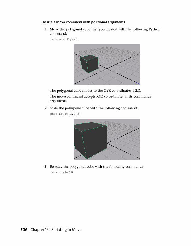
To use a Maya command with positional arguments
1 Move the polygonal cube that you created with the following Pythoncommand:
cmds.move(1,2,3)
The polygonal cube moves to the XYZ co-ordinates 1,2,3.
The move command accepts XYZ co-ordinates as its commandsarguments.
2 Scale the polygonal cube with the following command:
cmds.scale(2,2,2)
3 Re-scale the polygonal cube with the following command:
cmds.scale(3)
706 | Chapter 13 Scripting in Maya

When a command is not provided with enough command arguments,the command uses the default arguments. The polygonal cube X scale isset to three, but the Y and Z scale values are set to their default argumentone.
4 Delete the selected polygonal cube.
cmds.delete()
Using flags in PythonFlags are used with commands to modify their execution. Python implementsflags as named arguments. Some flags in MEL do not require values. As allnamed arguments in Python require a value, these flags are given the valueTrue to enable the flag, or False to ignore the flag. When setting multiplenamed arguments, argument-value pairs are separated by commas within thebrackets. Command arguments must appear before named arguments in acommand.
To use flags in Python
1 Create a polygonal cube with the width defined at creation time by typingthe following:
cmds.polyCube(width=5)
The width flag allows you to set the width of a cube at creation time.
Using flags in Python | 707

2 Create a polygonal sphere with the radius and subdivisions in X andname defined at creation time.
cmds.polySphere(radius=1, subdivisionsX=4, name="testSphere")
You can use multiple flags to modify the execution of a command byseparating the flag-value pairs with a comma. The radius flag sets theradius of the created sphere. The subdivisionsX flag sets the number ofsubdivisions in X for the sphere.
NOTE A list of flags available for a command can be output to the Scripteditor by typing cmds.help("command"). For example: cmds.help("sphere")
To use flags with command arguments in Python
1 Move the polygonal sphere by typing the following in the Script Editor:
cmds.move(2,2,2)
2 Select the polygonal cube.
3 Move the polygonal cube by typing the following:
cmds.move(1,2,3)
708 | Chapter 13 Scripting in Maya

4 Move the polygonal cube relative to its current position by typing thefollowing:
cmds.move(-1,0,-2,relative=True)
The polygonal cube moves relative to its current position. The relativeflag must be placed after the command arguments, as in Python, whenpassing arguments, named arguments must appear after positionalarguments. The command arguments must always be the first argumentsof the command.
5 Move the polygonal sphere without selecting it by typing the following:
cmds.move(3,2,1,"testSphere",relative=True)
The name of the object must be passed as a string after the commandarguments, but before the flags.
Using flags in Python | 709

To use flags with multiple arguments in Python
1 Create a yellow tinted point light by typing the following:
cmds.pointLight(rgb=(1,1,0.5))
The point light command creates a point light at the origin. The rgb flagspecifies the color of the light. The rgb flag require three values; red,green and blue.
When flags require multiple values, the values must be packed withinPython’s tuple or list data types. Tuples are a method of storing multipleitems of homogenous data within a single variable, similar to an arrayin MEL. The list is similar to the tuple, but supports multiple data typeswithin a single variable. The above command packs the RGB values intoa tuple. You could also use a list to achieve a similar effect.
2 Move the currently selected light by typing the following:
cmds.move(12,15,12)
3 Create a blue tinted light by typing the following:
cmds.pointLight(rgb=[0.2,0.2,1])
Square brackets [ ] indicate lists, and parentheses ( ) indicate tuples.
The values for the rgb flag can be packed into either a list or a tuple andperform the identical operation.
4 Move the currently selected light by typing the following:
cmds.move(12,15,-5)
5 Select the polygonal cube and polygonal sphere by clicking the polygonalcube, then shift clicking the sphere.
6 Frame the selected objects by pressing the f hotkey on your keyboard.
7 Render the scene by pressing the render current frame button onthe Status line.
The Render View opens and displays the following image.
710 | Chapter 13 Scripting in Maya
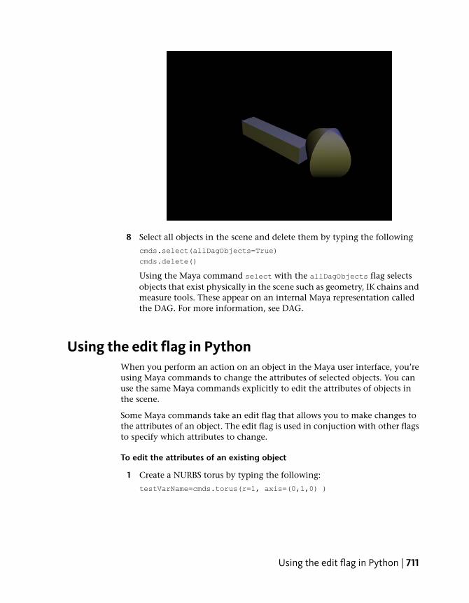
8 Select all objects in the scene and delete them by typing the following
cmds.select(allDagObjects=True)
cmds.delete()
Using the Maya command select with the allDagObjects flag selectsobjects that exist physically in the scene such as geometry, IK chains andmeasure tools. These appear on an internal Maya representation calledthe DAG. For more information, see DAG.
Using the edit flag in PythonWhen you perform an action on an object in the Maya user interface, you’reusing Maya commands to change the attributes of selected objects. You canuse the same Maya commands explicitly to edit the attributes of objects inthe scene.
Some Maya commands take an edit flag that allows you to make changes tothe attributes of an object. The edit flag is used in conjuction with other flagsto specify which attributes to change.
To edit the attributes of an existing object
1 Create a NURBS torus by typing the following:
testVarName=cmds.torus(r=1, axis=(0,1,0) )
Using the edit flag in Python | 711
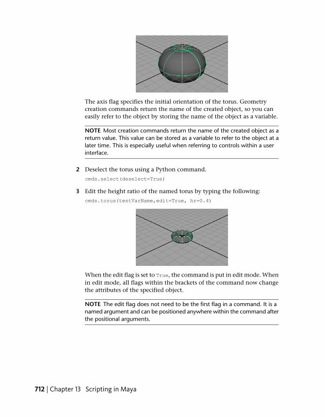
The axis flag specifies the initial orientation of the torus. Geometrycreation commands return the name of the created object, so you caneasily refer to the object by storing the name of the object as a variable.
NOTE Most creation commands return the name of the created object as areturn value. This value can be stored as a variable to refer to the object at alater time. This is especially useful when referring to controls within a userinterface.
2 Deselect the torus using a Python command.
cmds.select(deselect=True)
3 Edit the height ratio of the named torus by typing the following:
cmds.torus(testVarName,edit=True, hr=0.4)
When the edit flag is set to True, the command is put in edit mode. Whenin edit mode, all flags within the brackets of the command now changethe attributes of the specified object.
NOTE The edit flag does not need to be the first flag in a command. It is anamed argument and can be positioned anywhere within the command afterthe positional arguments.
712 | Chapter 13 Scripting in Maya
Communicating between Python and MELMEL and Python in Maya each have built in commands to communicate witheach other. MEL and Python communicate by calling commands in the otherlanguage and evaluating the results of the last executed command.
Python communicates with MEL using the eval() command. Unlike the otherPython commands in this lesson, the eval() function does not belong to theMaya commands module (maya.cmds). The eval() function belongs to themaya.mel module. The eval() function can call MEL scripts or execute MELcommands by sending the commands as a string. Multiple MEL commandscan be called in the string by separating the commands with semi-colons. ThePython eval() function returns the results of the last executed MEL script orcommand within the eval brackets.
MEL communicates with Python using the python command. The pythoncommand accepts a string as its only argument. The string is sent to Pythonto be evaluated, and the result is returned to MEL. As Python has a moredescriptive type system, some results from Python commands returned toMEL have their data type modified. For more information on type conversion,see MEL/Python communication of the Python guide.
To call MEL commands from Python
1 Select a Python tab in the Script Editor
2 Import the MEL module
import maya.mel
The maya.mel module is a module for evaluating MEL expressions inPython.
3 Call a MEL command by typing the following:
maya.mel.eval("sphere -radius 3;")
A sphere of radius three is created at the origin, just as if you had usedthe Python command.
4 Select a MEL Tab in the Script Editor
5 Declare a variable in the MEL tab by typing the following:
global float $MyMELVariable=22.7;
Only global MEL procedures, variables and scripts are accessible fromwithin Python.
6 Select a Python tab.
Communicating between Python and MEL | 713
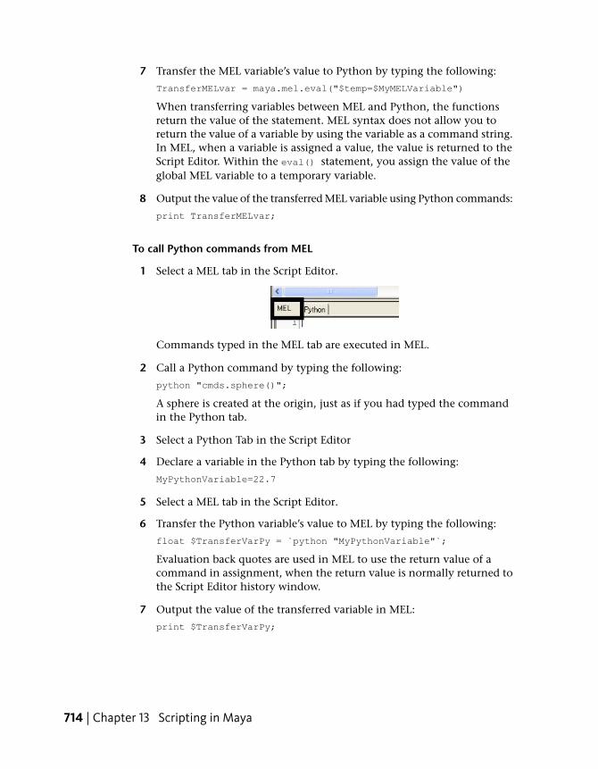
7 Transfer the MEL variable’s value to Python by typing the following:
TransferMELvar = maya.mel.eval("$temp=$MyMELVariable")
When transferring variables between MEL and Python, the functionsreturn the value of the statement. MEL syntax does not allow you toreturn the value of a variable by using the variable as a command string.In MEL, when a variable is assigned a value, the value is returned to theScript Editor. Within the eval() statement, you assign the value of theglobal MEL variable to a temporary variable.
8 Output the value of the transferred MEL variable using Python commands:
print TransferMELvar;
To call Python commands from MEL
1 Select a MEL tab in the Script Editor.
Commands typed in the MEL tab are executed in MEL.
2 Call a Python command by typing the following:
python "cmds.sphere()";
A sphere is created at the origin, just as if you had typed the commandin the Python tab.
3 Select a Python Tab in the Script Editor
4 Declare a variable in the Python tab by typing the following:
MyPythonVariable=22.7
5 Select a MEL tab in the Script Editor.
6 Transfer the Python variable’s value to MEL by typing the following:
float $TransferVarPy = `python "MyPythonVariable"`;
Evaluation back quotes are used in MEL to use the return value of acommand in assignment, when the return value is normally returned tothe Script Editor history window.
7 Output the value of the transferred variable in MEL:
print $TransferVarPy;
714 | Chapter 13 Scripting in Maya

TIP Transferring values between Python and Maya can also be accomplishedby using invisible user interface elements. You can edit and query the contentsof user interface elements with both scripting languages.
Beyond the lessonIn this lesson, you learned how to access Maya’s functionality through Pythonscripting commands. You can:
■ Type basic Python commands in the Script Editor to access MayaCommands.
■ Use named arguments as flags at object creation time to specify theattributes for the objects.
■ Use commands that require multiple arguments by packing the argumentsin a tuple or list.
■ Edit the attributes of objects using a command with the edit flag.
■ Execute Python commands from the MEL interpreter and execute MELcommands from the Python interpreter.
■ Transfer values between Python and MEL.
The MEL tutorials introduce some other uses for scripting in Maya. You canfollow through with the MEL tutorials by using the Python CommandReference to translate MEL commands to their Python equivalents.
Python can also be used to write scripted plug-ins. For more information, seeIntroduction to Maya Python API in the API guide.
Beyond the lesson | 715

716
Assets
Introduction
In Maya, a container is a special type of node that can be used to encapsulatesets of related nodes. A template is an external file that specifies a commoninterface that can be applied to multiple containers (for example, a containerof a car, a truck, and an ambulance all have similar components and can thuscan have a common interface) and accessed from the Maya UI. A container withan applied template is called an asset.
In complex scenes with many nodes and attributes, assets become a keyorganizational tool by allowing you to package nodes together and expose onlythe attributes you need. This allows you to keep all the Maya editors clean andclutter-free.
Assets also allows you to customize which attributes are shown to which userswhile simultaneously locking them out of other attributes. This allows you toensure the integrity of your scene even when others work on it.
Preparing for the lessonsTo ensure the lesson works as described, do these steps before beginning:
1 Select File > New Scene.
2 If you have not already done so, copy the GettingStarted folder from itsinstallation location to your projects directory. Then, set the
14
717

GettingStarted directory as your Maya project. For more information,see Copying and setting the Maya project on page 25.
3 As you work through these lessons, remember to save your workfrequently and increment the name of the file every so often (filename1,filename2, and so on).
In this way you’ll have earlier versions of your work to return to shouldthe need arise.
4 (Optional) Set the current project folder to the Assets tutorial folder byselecting File > Project > Set. Then navigate to the GettingStartedfolder, select the Assets folder and click OK.
Lesson 1: Setting up an asset
IntroductionIn this lesson, you create a container representing the provided fire truckmodel. You then publish attributes from each part and create a template todefine future emergency vehicles.
In this lesson you’ll be introduced to some of the asset options Maya providesby learning how to:
■ Place a polygon object into a container.
■ Publish attributes to the container.
■ Publish the root node transform to the container.
■ Set container-centric selection.
■ Create a template for the container.
Lesson setupTo ensure the lesson works as described, do the following steps beforebeginning:
1 Make sure you’ve done the steps in Preparing for the Lesson.
2 Open the scene file named FireTruck.mb.
718 | Chapter 14 Assets

This file can be found in the Getting Started directory that you set asyour Maya project:
Getting Started/Assets/Firetruck.mb
The scene contains a model of a fire truck split into various pieces suchas the body, axles, and doors.
Creating a containerA container is the first building block of an asset and is used to contain relatednodes in your scene. A container is not visible in the main viewport, but youcan select it from the Outliner, Hypergraph Connections editor, and AssetEditor.
In this case, all the fire truck components (including lights) are groupedtogether. This is important because you want the fire truck components tomove together when animated. Thus, the fire truck group node is the centralnode to the container, and thus will become the container’s root node.
To create a container for the fire truck
1 Select Fire_truck_GRP in the Outliner.
2 Select Assets > Create Container > .
The Create Container options window appears.
Creating a container | 719

3 In the Create Container options window, select Edit > Reset Settings.
4 Under Create Container Effect, set the Name to Fire_truck_CNT.
5 Under the Include Options, turn on Include Shaders and IncludeHierarchy, and set the hierarchy to Below (including shapes).
Setting these options ensures that everything the firetruck needs tomaintain its current appearance is packaged into the container.
6 In the Publish Options, turn on Root Transform and Root Attributes.
Setting these two options automatically publishes Fire_truck_GRP as thecontainer’s root node (thus allowing it to be a parent or child in a scene)and publishes its attributes to the container so that they can be tweakedfrom the container’s interface.
7 Click Apply and Close.
Maya encapsulates the fire truck in a container.
Publishing attributes
Now that the fire truck is encapsulated, you can publish attributes from theindividual pieces to make them available at the container level.
A published attribute on a container is bound to an attribute of the objectinside. When a user changes the published attribute’s value, the value of thecorresponding internal attribute is changed as well. You can choose to publish
720 | Chapter 14 Assets

all or only a subset of the available internal attributes, allowing you to limithow much access a user has to the object contained inside.
The published attributes of a container are often referred to as the container’sinterface, and is useful because it allows you access to every important controlfor your asset in a single place.
To organize objects under their containers
➤ In the Outliner, select Display > Container Contents > Under Container.
Now Fire_truck_GRP and its children appear under the Fire_truck_CNTobject.
To publish the right cab door
1 In the Outliner, expand Fire_truck_CNT by clicking next to its name.
Fire_truck_GRP appears under Fire_truck_CNT.
2 Expand Fire_truck_GRP, then Doors_GRP.
3 Select Cab_door_f_r_GRP and open the Channel Box by clicking .
4 In the Channel Box, under the Cab_door_f_r_GRP heading, Ctrl +
right-click the label Door Open and select Publish to Container > from the marking-menu.
The Publish Attribute Options window appears.
5 In the Publish Attribute Options window, select Edit > Reset Settings.
6 In the Attribute name section, select Custom name and then typeFront_Right_Door in the Custom name field.
The name Front Right Door represents the published name for thisattribute and represents the door’s rotation in the fire truck container’sinterface.
7 Click Apply.
The Front Right Door attribute now appears in the Fire_truck_CNT sectionof the Channel Box.
Now, in the Attribute Editor or Channel Box you can input values intothe Front Right Door field to open and close the door. Notice that as youchange the value, the value of door_open under Doors_GRP changes tomatch. This is because your published name (Front_Right_door) is bound
Publishing attributes | 721

to the Rotate Y attribute of Cab_door_f_r_GRP. When one changes, bothare updated.
8 Repeat steps 3 - 7 to publish the following:
Published nameNode Name
Front_Left_DoorCab_door_f_l_GRP
Rear_Right_DoorCab_door_r_r_GRP
Rear_Left_DoorCab_door_r_l_GRP
9 Select Edit > Reset Settings.
10 Click Close.
NOTE The Door Open attribute for each door is a custom attribute that controlsthe Y rotation of each door. Although you could publish the rotate Y attribute ofeach door directly, these custom attributes are provided so that each door opensas the value increases from 0 to 1. Without these attributes, some doors wouldopen as their rotation increases and others would open as their rotation decreases.
You will learn how to create a custom attribute in the next section.
Publishing multiple attributes to a single published name
722 | Chapter 14 Assets

Unlike the doors, a fire truck’s wheels are expected to move together. Forexample, the wheels on the front and back axles should spin together, andthe front wheels should turn together. To do this, you need to create a customattribute to control both components at once. Then you can publish yourcustom attribute to the container.
To turn the front wheels together
1 In the Outliner, expand Axles_GRP, then select Wheels_GRP.
2 Open the Attribute Editor by clicking .
3 Make sure the Wheels_GRP tab is currently active, then in the AttributeEditor, select Attributes > Add Attributes.
The Add Attribute window appears.
4 Under Numeric Attribute Properties, set Long Name to Front_wheel_turn.
5 Set Minimum to -30 and Maximum to 30.
6 Click Add.
Maya adds the new attribute to Wheels_GRP in the Extra Attributes sectionof the Attribute Editor. The Add Attribute window stays open.
7 Repeat steps 4 to 6 setting Long Name to Wheel_spin. Do not set aMinimum/Maximum value for this attribute.
8 Click Close.
Your custom attributes can be found in the Extra Attributes section of theAttribute Editor. However, if you modify their values, nothing happens. Thisis because you have not connected them to anything yet.
To make the front wheels turn together
1 Open the Connection Editor by selecting Windows > General Editors >Connection Editor.
2 In the Connection Editor, Wheels_GRP should already be displayed inthe Output section. If it is not, select Wheels_GRP in the Outliner andclick Reload Left in the Connections Editor.
NOTE If Outputs does not appear over the left column in the ConnectionsEditor, click the to <- from button to reset its position.
Publishing multiple attributes to a single published name | 723

3 Scroll to the bottom of the left column and select Front_wheel_turn.
4 In the Outliner, expand Wheels_GRP and select Wheel_f_l_GRP.
5 In the Connection Editor, click Reload Right.
The right column is filled with the left wheel’s attributes.
6 In the right column, expand rotate and select rotateY.
rotateY turns to italics to signify that it has been connected.
7 In the Outliner, select Wheel_f_r_GRP and repeat steps 5 and 6.
If you adjust the value of Front_wheel_turn, both front wheels turn together.
Next you need to make the front and rear wheels spin in unison.
To make the front and back wheels spin together
1 In the Connection Editor, select Wheel_Spin in the left column androtateX in the right column.
2 In the Outliner, select Wheel_f_l_GRP.
3 In the Connection Editor, click Reload Right.
4 In the right column, expand rotate and select rotateX.
724 | Chapter 14 Assets
5 Repeat steps 2-4 for the other 3 wheels.
Now if you adjust the value of the wheel_spin attribute in the Attribute Editoror Channel Box, all four wheels spin in unison. Although, in some cases, it’suseful for the front and back wheels to be able to spin at different rates, thecurrent setup is fine for this tutorial.
Now you can publish your custom attribute to the container. You can do thisdirectly from the Attribute Editor.
To publish the wheel turn and wheel spin
1 In the Attribute Editor, right-click Front Wheel Turn and select Publishto ‘Fire_truck_CNT’ from the marking menu.
2 Right-click Wheel Spinand select Publish to ‘Fire_truck_CNT’ from themarking menu.
Both attributes are published to the fire truck container with the samepublished names as their corresponding custom attributes.
Open the second scene for the lessonTo ensure the lesson works as described, do the following steps beforebeginning:
➤ Open the scene file named FireTruck_published.mb.
This file can be found in the Getting Started directory that you set asyour Maya project:
Getting Started/Assets/Firetruck_published.mb
The scene contains the same fire truck model but with a complete set ofpublished attributes.
Creating a templateOnce you’ve published all your attributes, you can create a template fromyour asset. A template defines which published attributes an asset needs to beconsidered complete. You can then re-purpose this template for use withfuture fire truck models, or in our case, any emergency vehicle.
To create a template, you first need to open the Asset Editor.
Open the second scene for the lesson | 725

To open the Asset Editor
1 In the Outliner, select Fire_truck_CNT.
2 Select Assets > Asset Editor.
The Asset Editor appears.
The Asset Editor allows you to manage all the containers and templates inyour scene from a single interface. From the Asset Editor you can publish andunpublish attributes, change published names, bind and unbind attributes topublished names, and create templates and views.
The Asset Editor is divided into two columns. The left column shows you allthe containers in your scene in a format similar to the Outliner. The rightcolumn shows you all the published names associated with a container. Inorder to see the published names for a container, you have to pin a containerfirst.
To pin the fire truck container
1 Select Fire_truck_CNT in the left column.
2 Click the pin icon ( ).
The fire truck’s published names appear in the right column.
Now that you’ve pinned the fire truck container, you are ready to create atemplate.
To create a template
1 In the Asset Editor, select Template > Save As.
A file browser appears.
2 Navigate to the assets folder.
3 Set the File name to emergency_vehicle.
4 Click Save.
Maya creates a template file.
Notice that once you create a template file, the small arrows next to thepublished names in the right column change from red to green. This signifiesthat these published names come from the template and are currently bound.
726 | Chapter 14 Assets

Creating ViewsOne advantage to creating a template for your asset is that you can createmultiple Views for it. You can use Views to customize which attributes certainusers can see in the Maya editors. For example, you can create a View thatlimits an animator to only the door controls and wheel spin controls andanother View to limit a shader to only the truck’s body materials and textures.
Not only do Views cut down the amount of editor clutter for each artist, butit also adds a layer of protection so that users don’t accidentally change anattribute they shouldn’t have control over.
To create a View for an animator
1 In the Asset Editor, select View > Add > .
The Add View Options window appears.
2 Select Edit > Reset Settings.
3 Set the Name to Animator.
4 Set Layout Mode to Flat.
5 Click Apply and Close.
Maya creates a new View for the asset.
Notice that even though you created a new View, all the attributes are stillvisible in the right column. Since we only want the animation controls visible,we need to customize this View.
To customize a View
1 Open the Script Editor by clicking .
NOTE If you prefer, you can also use any external text editing tool to performthe following steps.
2 In the Script Editor, select File > Load Script.
A file browser appears.
3 Set Files of type to All types.
4 Navigate to the Assets folder and select emergency_vehicle.template.
Creating Views | 727

5 Click Open.
The template is now displayed in the Script Editor. The template is anXML file and thus is arranged with a series of tags.
6 Scroll to the bottom of the Script Editor until you find the tag
<view name='Animator' template='emergency_vehicle'>
Underneath this tag, delete the following:
■ <property name='headlight_intensity'/>
■ <property name='siren_intensity'/>
■ <property name='interior_light_intensity'/>
■ <property name=’transMinusRotatePivot’/>
7 Highlight the text of the XML file or press Ctrl + A.
8 Select File > Save Script.
A file browser appears.
9 Set Files of type to All types.
10 Navigate to the Assets folder and select emegency_vehicle.template.
11 Click Save.
12 Close the Script Editor.
You’ve now customized the View by leaving only the attributes an animatorwould be interested in. However, this is still not reflected in the Asset Editor.To see your changes, you need to refresh to the Asset Editor.
To update the Asset Editor
➤ Select Template > Reload.
The right panel updates to show you your customized View.
Now repeat the procedure to create a Shader view, but with the followingchanges:
■ Set the template Name to Lighter.
■ When viewing the template in the Script Editor, scroll down to<view name='Lighter' template='emergency_vehicle'>
728 | Chapter 14 Assets

And remove the following:
■ <property name='translate'/>
■ <property name='rotate'/>
■ <property name='scale'/>
■ <property name='visibility'/>
■ <property name =’Front_R_Door_Open’/>
■ <property name='Front_L_Door_Open'/>
■ <property name='Rear_R_Door_Open'/>
■ <property name='Rear_L_Door_Open'/>
■ <property name='front_wheel_turn'/>
■ <property name='wheel_spin'/>
■ <property name=’transMinusRotatePivot’/>
■ <property name='toggle_headlights'/>
■ <property name='toggle_front_flashers'/>
■ <property name='toggle_rear_flashers'/>
■ <property name='toggle_sirens'/>
■ <property name='toggle_interior_light'/>
Now you have two different Views that are useful for two different artists. Youcan switch between Views in the Asset Editor by selecting View > Name, andthen selecting the name of the View you want to set.
Creating Views | 729

Notice that in both views, the Trans Minus Rotate Pivot attribute is hidden.This is another great use for views, they allow you to hide attributes thatcannot or should not ever be modified manually, but still need to be published(for reasons that are evident in Lesson 2).
You can now close the Asset Editor and save your file.
Assigning a custom iconCurrently, Fire_truck_CNT is displayed in the Outliner and Hypergraph withthe standard container icon. You can customize this icon to make the containermore obvious when you place the fire truck in a scene with more than onecontainer.
To customize the container icon
1 Select Fire_truck_CNT in the Outliner.
2 In the Attribute Editor, under the Fire_truck_CNT tab, open the ContainerAttributes section.
This section displays all of the container’s own attributes.
3 Click the file icon button next to Icon Name.
730 | Chapter 14 Assets

A file browser appears.
4 Navigate to Getting Started/Assets/sourceimages/xpm and selectfire_truck_icon.xpm.
5 Click Open.
The image changes to a small fire truck icon.
Setting Black Box modeAlthough Views encourage certain users to only modify certain attributes, itis still possible for a user to inadvertently access and change attributes thatthey shouldn’t. To greatly increase the integrity of your asset, you can set itto Black Box mode.
When Black Box mode is turned on, users can only see the container itselfand all of its published attributes and published nodes. A user cannot open acontainer in the Outliner, Hypergraph, or other editors, to view theunpublished attributes and unpublished nodes inside. An additional benefitof this is that it greatly decreases the complexity of scenes in editors since itreduces entire trees of objects to a single object.
To turn on Black Box mode
1 In the Outliner, select Fire_truck_CNT.
2 In the Attribute Editor, in the Container Attributes section, turn on BlackBox.
Now if you look at the Outliner, the expand icon next to Fire_truck_CNT hasdisappeared. If you try clicking it, Maya does not allow you to expand it tosee its children.
Setting Black Box mode | 731

Beyond the lessonIn this lesson you learned how to encapsulate objects into an asset.
■ You can create a container that encapsulates existing objects in the scene.
■ You can publish attributes to a container.
■ You can create custom attributes, connect them to objects in the scene,and then publish those custom attributes.
■ You can use the Asset Editor to create a template for an existing asset.
■ You can create and customize Views of an asset.
■ You can assign a custom icon to an asset.
■ You can set an asset to Black Box mode to hide its unpublished contents.
Lesson 2: Using assets in a scene
IntroductionIn this lesson you first learn how to import existing assets into a scene. Youthen apply the emergency vehicle template you created in Lesson 1: Settingup an asset to a police car in the scene and then use the matching published
732 | Chapter 14 Assets

attributes to replace it with your fire truck. You then reference a fire into thescene and finish dressing the scene with a number of external assets.
In this lesson you learn how to:
■ Apply an existing template to a container.
■ Bind container attributes to a template’s published names.
■ Reference an asset in another file with File Referencing.
■ Transfer values from one asset to another.
■ Use container proxies to dress a scene.
Lesson setupTo ensure the lesson works as described, do the following steps beforebeginning:
1 Make sure you’ve done the steps in Preparing for the Lesson.
2 Open the scene file named EmergencyCity.mb.
This file can be found in the Getting Started directory that you set asyour Maya project:
Getting Started/Assets/EmergencyCity.mb
The scene contains a model of a city block and a police car. If you playback the animation, the police car drives along the road, stops outsideone of the apartment buildings, and opens its front doors.
Lesson setup | 733
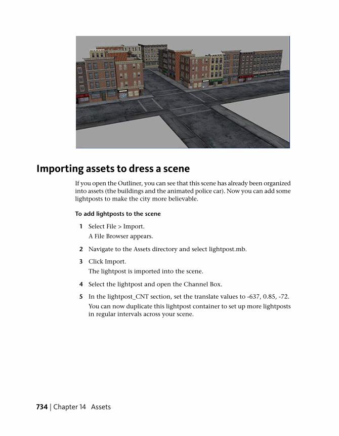
Importing assets to dress a sceneIf you open the Outliner, you can see that this scene has already been organizedinto assets (the buildings and the animated police car). Now you can add somelightposts to make the city more believable.
To add lightposts to the scene
1 Select File > Import.
A File Browser appears.
2 Navigate to the Assets directory and select lightpost.mb.
3 Click Import.
The lightpost is imported into the scene.
4 Select the lightpost and open the Channel Box.
5 In the lightpost_CNT section, set the translate values to -637, 0.85, -72.
You can now duplicate this lightpost container to set up more lightpostsin regular intervals across your scene.
734 | Chapter 14 Assets
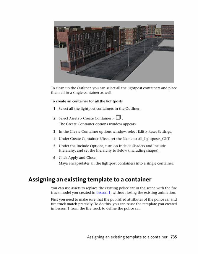
To clean up the Outliner, you can select all the lightpost containers and placethem all in a single container as well.
To create an container for all the lightposts
1 Select all the lightpost containers in the Outliner.
2 Select Assets > Create Container > .
The Create Container options window appears.
3 In the Create Container options window, select Edit > Reset Settings.
4 Under Create Container Effect, set the Name to All_lightposts_CNT.
5 Under the Include Options, turn on Include Shaders and IncludeHierarchy, and set the hierarchy to Below (including shapes).
6 Click Apply and Close.
Maya encapsulates all the lightpost containers into a single container.
Assigning an existing template to a containerYou can use assets to replace the existing police car in the scene with the firetruck model you created in Lesson 1, without losing the existing animation.
First you need to make sure that the published attributes of the police car andfire truck match precisely. To do this, you can reuse the template you createdin Lesson 1 from the fire truck to define the police car.
Assigning an existing template to a container | 735

NOTE If you did not start at Lesson 1, both the fire truck model and template canbe found in the Getting Started/Assets/assets folder.
To assign a template to a container
1 Select Assets > Asset Editor.
The Asset Editor appears.
2 In the left column of the Asset Editor, select police_car_CNT.
3 Click the pin icon ( ).
4 Select Template > Assign > Assign New Template.
A file browser appears.
5 Navigate to the emergency_vehicle.template file you created in Lesson 1and select it.
If you didn’t start at Lesson 1, navigate to GettingStarted/Assets/assets/templates and select the fileemergency_vehicle.template.
736 | Chapter 14 Assets

6 Click Select.
A number of the attribute icons turn green, while others turn yellow. Tobetter organize this, you can apply the template’s views.
7 View > Mode > Use Template.
The right panel is split into a number of sections.
The majority of the attribute icons in the police_car_CNT section aregreen. This signifies that they have been bound to identical publishednames that were found in the template.
However, there are a set of published names without icons next to them. Theserepresent published names that the template is expecting, but couldn’t find.In some cases this may mean you need to bind and publish additionalattributes to fulfill them.
NOTE The icons in the Published Nodes section appear yellow because templatesdo not recognize published nodes.
Assigning an existing template to a container | 737

Binding attributesIn order for your asset to be considered valid, every published name in thepolice_car_CNT section must be bound to an attribute of the police car.Currently, the transMinusRotatePivot attributes are not bound, so the templateis invalid. To fulfill this template, you must bind them manually.
To bind the doors
1 In the left panel of the Asset Editor, click the square expand icon ( ).
The contents of the container appears.
2 Click the circular expand icon ( ) next to police_car_GRP.
A list of the node’s attributes appears.
NOTE If you do not see the circular expand icons ( ), make sure thatDisplay > Attributes (Channels) is turned on in the Asset Editor.
3 Scroll down and click the circular expand icon ( ) next to the TransMinus Rotate Pivot attribute.
738 | Chapter 14 Assets
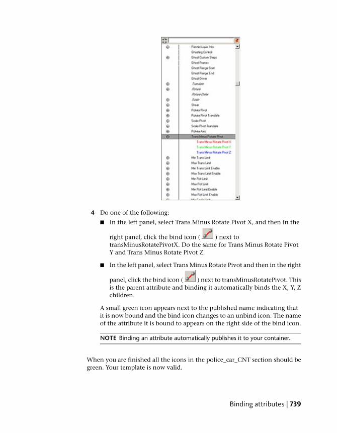
4 Do one of the following:
■ In the left panel, select Trans Minus Rotate Pivot X, and then in the
right panel, click the bind icon ( ) next totransMinusRotatePivotX. Do the same for Trans Minus Rotate PivotY and Trans Minus Rotate Pivot Z.
■ In the left panel, select Trans Minus Rotate Pivot and then in the right
panel, click the bind icon ( ) next to transMinusRotatePivot. Thisis the parent attribute and binding it automatically binds the X, Y, Zchildren.
A small green icon appears next to the published name indicating thatit is now bound and the bind icon changes to an unbind icon. The nameof the attribute it is bound to appears on the right side of the bind icon.
NOTE Binding an attribute automatically publishes it to your container.
When you are finished all the icons in the police_car_CNT section should begreen. Your template is now valid.
Binding attributes | 739

NOTE You could also fulfill the template by selecting the container and thenselecting Assets > Publish Connections. This publishes all incoming and outgoingconnections to and from your container and binds them to appropriate publishednames. However, this option also publishes extra attributes which you do notnecessarily need published in this case. In most cases it is up to you to decidewhich method works better for your given situation.
Swapping assetsAssets with partial or fully identical sets of published names can be swappedwhile maintaining the values of the matching published attributes. This allowsyou to quickly re-purpose scenes or swap different assets in and out of yourcurrent scene.
To swap the police car for a fire truck
1 Select File > Import.
A file browser appears.
2 Navigate to the Fire truck file that you saved in Lesson 1.
740 | Chapter 14 Assets

If you didn’t start at Lesson 1, navigate to GettingStarted/Assets/assets and select the file firetruck_templated.mb.
Maya imports the fire truck into your scene.
3 In the Outliner, select police_car_CNT and Ctrl + select fire_truck_CNT.
4 Select Edit > Transfer Attribute Values > .
The Transfer Attribute Values Options window appears.
5 In the Transfer Attribute Values Options window, select Edit > ResetSettings.
6 Turn on Values.
7 Turn on In connections and set it to Transfer from source.
8 Turn on Out connections.
9 Click Apply and Close.
The fire truck jumps to the police car’s position so that they overlap. If youplay the animation now, the fire truck follows the police car’s previous pathand then stops outside the apartment building and opens its doors. The policecar remains stationary.
Swapping assets | 741

You can now delete the police car asset from the scene by selecting it in thescene and pressing Delete. Remember to delete the container from the Outlinerafterward.
Referencing assets in a sceneIn the previous section you imported a fire truck asset directly into the scene.However, you can also reference assets from other files. File referencing allowsyou to represent an object from another file in your scene without actuallyimporting that file.
References do not use as much memory as full imports, and have the addedbenefit of allowing you to tweak referenced material in their source files, andhave the referenced material automatically update in your main file. Thisallows multiple people to work on different pieces of a single scenesimultaneously.
To reference an asset
1 Select File > Reference Editor.
The Reference Editor window appears.
2 In the Reference Editor, select File > Create Reference > .
3 Select Edit > Reset Settings.
4 Click Reference.
742 | Chapter 14 Assets
A file browser appears.
5 Navigate to Getting Started/Assets/assets and select police_car.mb.
6 Click Reference.
An entry appears in the Reference Editor. This represents the police car. Youcan turn the reference on and off by clicking the check box next to thereference name.
Now you can move the police car asset to the appropriate spot in your scene.Up until now, you’ve been using the Outliner to select your containers.However, you can change the selection method so that you can select themin your scene.
To turn on container centric selection
1 Select Window > Settings/Preferences > Preferences.
The Preferences window appears.
2 In the select the Selection section under Settings.
3 Turn on Container centric selection.
4 Click Save.
Now if you click on any part of the police car in the main scene, Maya selectsthe object’s container.
Now select the Move Tool and move the police car to the edge of one of thestreets in the scene. Using the same procedure outlined above, reference thesame police car file 3 more times and arrange the police cars around the scene,but not in the path of the fire truck.
Referencing assets in a scene | 743

Now you need a reason for all the emergency vehicles crowding around.
To reference a fire asset
1 In the Reference Editor, select File > Create Reference > .
2 Click Reference.
A file browser appears.
3 Navigate to Getting Started/Assets/assets and select flames.mb.
4 Click Reference.
5 Use the Move Tool to position the explosion a window on the buildingthat the fire truck stops at. You can also use the Rotate Tool to angle thefire out towards the street.
Now if you play the scene, the apartment burns before the fire truck arrives.
744 | Chapter 14 Assets
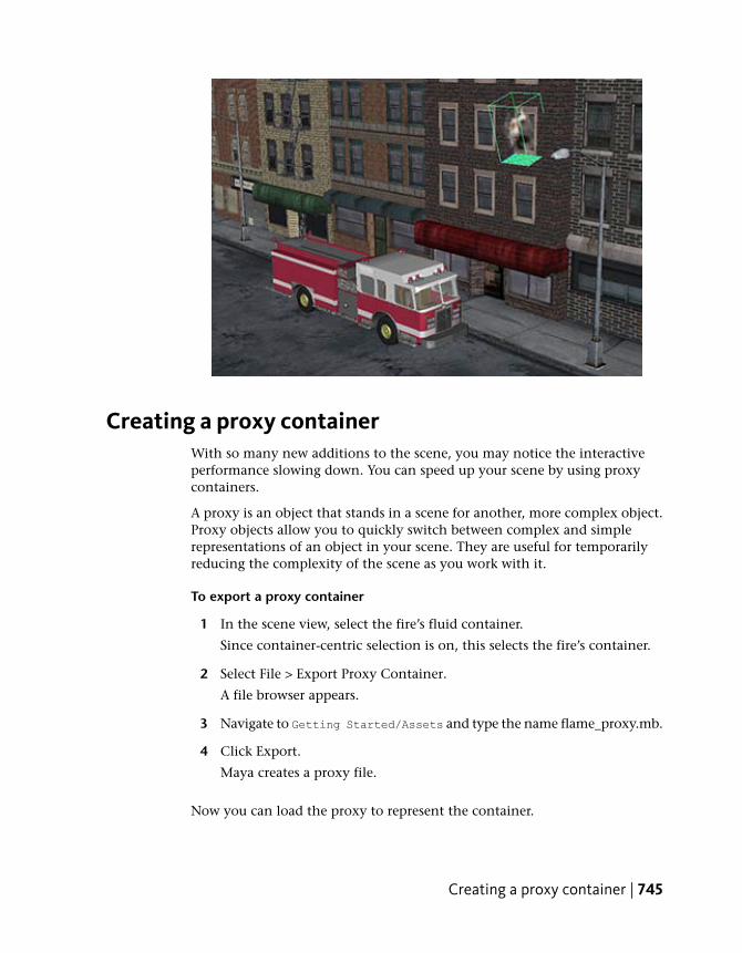
Creating a proxy containerWith so many new additions to the scene, you may notice the interactiveperformance slowing down. You can speed up your scene by using proxycontainers.
A proxy is an object that stands in a scene for another, more complex object.Proxy objects allow you to quickly switch between complex and simplerepresentations of an object in your scene. They are useful for temporarilyreducing the complexity of the scene as you work with it.
To export a proxy container
1 In the scene view, select the fire’s fluid container.
Since container-centric selection is on, this selects the fire’s container.
2 Select File > Export Proxy Container.
A file browser appears.
3 Navigate to Getting Started/Assets and type the name flame_proxy.mb.
4 Click Export.
Maya creates a proxy file.
Now you can load the proxy to represent the container.
Creating a proxy container | 745
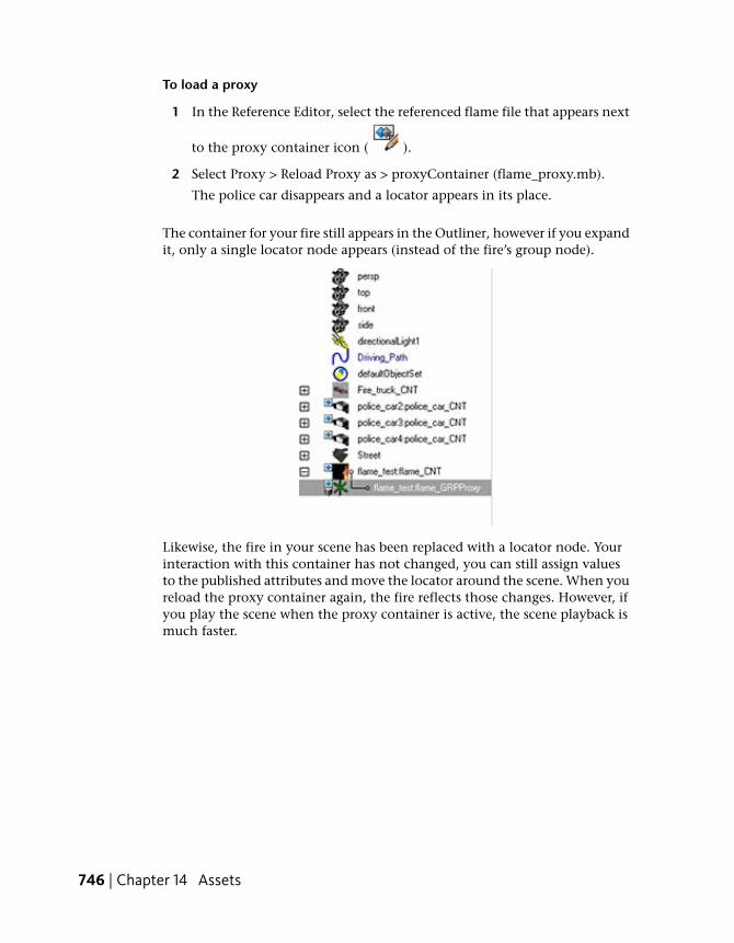
To load a proxy
1 In the Reference Editor, select the referenced flame file that appears next
to the proxy container icon ( ).
2 Select Proxy > Reload Proxy as > proxyContainer (flame_proxy.mb).
The police car disappears and a locator appears in its place.
The container for your fire still appears in the Outliner, however if you expandit, only a single locator node appears (instead of the fire’s group node).
Likewise, the fire in your scene has been replaced with a locator node. Yourinteraction with this container has not changed, you can still assign valuesto the published attributes and move the locator around the scene. When youreload the proxy container again, the fire reflects those changes. However, ifyou play the scene when the proxy container is active, the scene playback ismuch faster.
746 | Chapter 14 Assets

Modifying a proxy containerAlthough the locator in the scene gives you the position of your referencedasset, it doesn’t accurately convey the size or shape of the object it represents.You can modify the proxy file to give the proxy container a more useful shape.
To modify the proxy container
1 Save your current scene file.
2 Select File > Open Scene.
A file browser appears.
3 Navigate to Getting Started/Assets and select flame_proxy.mb.
4 Click Open.
Maya opens the proxy file.
The proxy file consists of a single locator at the center of the scene. Youcan add geometry to this file to customize the representation of the fire.
5 Select Create > Polygon Primitives > Cube > .
NOTE Make sure Interactive Creation is turned off in the Create > PolygonPrimitives menu.
The Create Polygon Cube window appears.
Modifying a proxy container | 747
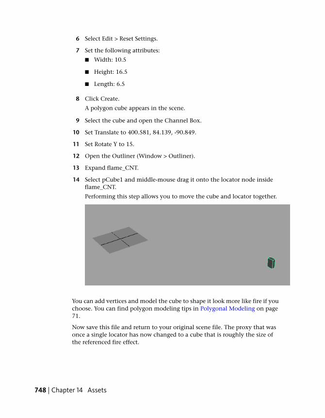
6 Select Edit > Reset Settings.
7 Set the following attributes:
■ Width: 10.5
■ Height: 16.5
■ Length: 6.5
8 Click Create.
A polygon cube appears in the scene.
9 Select the cube and open the Channel Box.
10 Set Translate to 400.581, 84.139, -90.849.
11 Set Rotate Y to 15.
12 Open the Outliner (Window > Outliner).
13 Expand flame_CNT.
14 Select pCube1 and middle-mouse drag it onto the locator node insideflame_CNT.
Performing this step allows you to move the cube and locator together.
You can add vertices and model the cube to shape it look more like fire if youchoose. You can find polygon modeling tips in Polygonal Modeling on page71.
Now save this file and return to your original scene file. The proxy that wasonce a single locator has now changed to a cube that is roughly the size ofthe referenced fire effect.
748 | Chapter 14 Assets
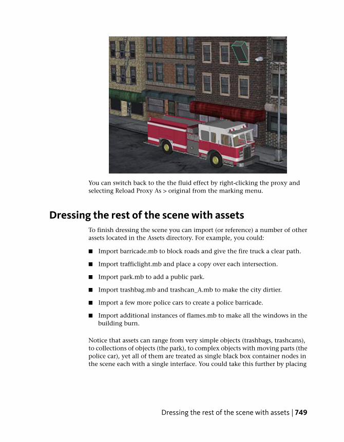
You can switch back to the the fluid effect by right-clicking the proxy andselecting Reload Proxy As > original from the marking menu.
Dressing the rest of the scene with assetsTo finish dressing the scene you can import (or reference) a number of otherassets located in the Assets directory. For example, you could:
■ Import barricade.mb to block roads and give the fire truck a clear path.
■ Import trafficlight.mb and place a copy over each intersection.
■ Import park.mb to add a public park.
■ Import trashbag.mb and trashcan_A.mb to make the city dirtier.
■ Import a few more police cars to create a police barricade.
■ Import additional instances of flames.mb to make all the windows in thebuilding burn.
Notice that assets can range from very simple objects (trashbags, trashcans),to collections of objects (the park), to complex objects with moving parts (thepolice car), yet all of them are treated as single black box container nodes inthe scene each with a single interface. You could take this further by placing
Dressing the rest of the scene with assets | 749
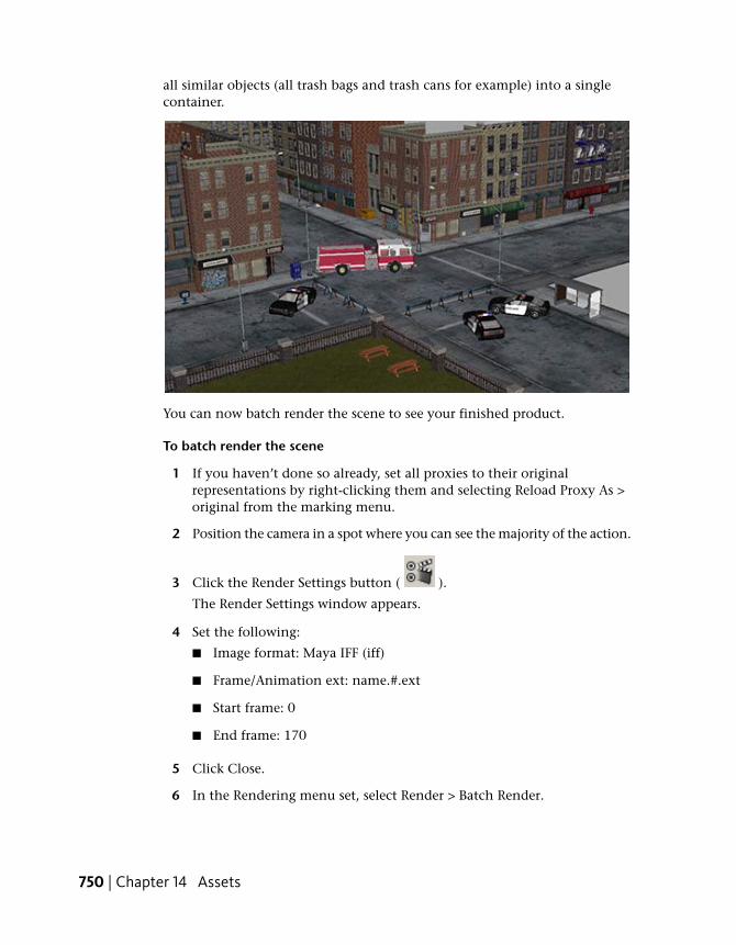
all similar objects (all trash bags and trash cans for example) into a singlecontainer.
You can now batch render the scene to see your finished product.
To batch render the scene
1 If you haven’t done so already, set all proxies to their originalrepresentations by right-clicking them and selecting Reload Proxy As >original from the marking menu.
2 Position the camera in a spot where you can see the majority of the action.
3 Click the Render Settings button ( ).
The Render Settings window appears.
4 Set the following:
■ Image format: Maya IFF (iff)
■ Frame/Animation ext: name.#.ext
■ Start frame: 0
■ End frame: 170
5 Click Close.
6 In the Rendering menu set, select Render > Batch Render.
750 | Chapter 14 Assets

Maya batch renders the scene. This may take a few minutes. You canmonitor the progress in the Status Line.
When the batch render is complete, you can view the sequence by selectingFile > View Sequence, and then opening the first file of the sequence (it hasan extension of .001). Maya then plays back the sequence of rendered imagesshowing you the final animation.
Beyond the lessonIn this lesson you learned how to incorporate assets into a scene.
■ You can use an existing template to define an asset.
■ You can swap one asset for another.
■ You can reference assets into a scene and instance them multiple times.
■ You can create proxy containers to stand in for referenced assets.
■ Imported additional assets to dress the scene.
Beyond the lesson | 751

752

Hair
Introduction
With Maya® HairTM, you can create a dynamic hair system to model realistichairstyles and hair behavior.
Since Hair is a generic dynamic curve simulation, you can also use these curvesto create non-hair effects, including ropes, chains, a suspension bridge, seacreatures, or lofted surface from a curve.
With Hair you can simulate:
■ natural movement and collisions of long hair
■ hair blowing in the wind or being blow dried
15
753

■ hair when swimming underwater
■ various hairstyles, including ponytails, braids, and updos
■ other dynamic curve effects such as ropes, chains, cables, wires, etc.
A hair system is a collection of hair follicles.
A hair follicle in human hair typically hosts one hair, whereas in Maya eachhair follicle hosts a hair curve. The hair follicle controls the attributes and curvesassociated with a particular hair clump, and how the hairs attach to a NURBSor polygonal surface. The input to each follicle is a Start Position NURBS curve,a surface and a UV position to attach to.
When creating hair, the hair system output can be in the form of NURBS curves,Maya® Paint EffectsTM strokes, or both. If the specified output when creatinghair is NURBS Curves, each follicle will contain one NURBS curve thatrepresents the position of the hair in that follicle. If the specified output isPaint Effects, each follicle has a hair clump, made up of Paint Effects strokes.
There are various attributes on a hair system for modifying the look andbehavior of the hair as a whole. There are also follicle level attributes that willoverride the hair system attributes; the visible result will be affected by boththe follicle and hair system attributes.
You can have more than one hair system on the same surface.
With the Paint Hair Tool you can create new hair systems, add and removefollicles, as well as paint hair attributes, including Clump Width Scale, Stiffness,and Braid.
Paint Effects hair can be rendered using the Maya Software renderer. You canalso convert Paint Effects hair to polygons and render in another renderer,such as mental ray® for Maya®. Or you can output just the dynamic NURBScurves to an external renderer, such as Renderman.
Consider outputting to Paint Effects if you want to:
■ render with the Maya Software renderer
■ convert the Paint Effects hair to polygons and render in any renderer
Consider outputting to NURBS curves if you want to:
■ use the curves as path or control curves for any standard Paint Effectsbrush, such as feathers or vines. These brushes behave differently than thedefault built in Paint Effects as the curves are not the hairs, but controls
754 | Chapter 15 Hair

that interpolate and affect Paint Effects. This scenario is slower to updateand takes a bit of time to set up.
■ select a few Current Position curves and loft a surface through them withconstruction history.
■ extrude a circle down the curve to create a tube.
■ use the curves for output to another renderer that directly supports curverendering.
Consider outputting to both NURBS curves and Paint Effects if you want to:
■ use both the curves (for example, as particle emitters to simulate sprayflying off wet hair) and render using the integrated Paint Effects eitherdirectly or by converting to polygons.
About hair simulationThis is the general workflow to create and animate hair:
■ create hair on models
■ style hair curves
■ modify hair attributes
■ set up hair shading/shadowing
■ render the scene
This chapter includes these lessons:
■ Lesson 1 Creating a basic hairstyle: Introduction on page 756
■ Lesson 2 Creating a dynamic non-hair simulation: Introduction on page777
Preparing for the lessonsTo ensure the lesson works as described, do these steps before beginning:
1 Make sure you understand the basic concepts of modeling NURBS curves,animation, and dynamics. For more information, see Maya Help.
About hair simulation | 755
2 Select the Dynamics menu set.
Unless otherwise noted, the procedures in these lessons assume theDynamics menu set is selected.
3 Select File > New Scene to create a new scene before you start each lesson.For those scenes that require you to open a file, the Hair scene files arelocated in GettingStarted/scenes directory. The GettingStarteddirectory is installed in the same location as your Maya softwareapplication.
4 Select Window > Settings/Preferences > Preferences. Click Timeline underCategories and make sure the Playback Speed is set to Play every frame.Dynamic animation plays more accurately with this setting.
Also set the playback and animation end times to 10000. This ensuresyou have lots of time to interact with the playback of the hair simulation.
5 If you have not already done so, copy the GettingStarted folder fromits installation location to your projects directory. Then, set theGettingStarted directory as your Maya project. For more information,see Copying and setting the Maya project on page 25 in the GettingStarted with Maya guide.
6 We also provide a completed scene for each of the lessons in this chapter.If you want to see the expected results of the lessons, you can open thescenes located in the GettingStarted/Hair directory. The scene filenamesend with Finish.mb, for example, hairFinish1.mb.
Lesson 1: Creating a basic hairstyle
IntroductionYou can create hair on NURBS and polygonal surfaces. For polygons, UVsshould be non-overlapping and fit between 0 and 1. Automatic mapping is aquick way to achieve this. (See Automatic UV mapping in the Mapping UVsGuide in the Maya Help.) In this lesson you are creating hair on a head model.
There are three sets of curves for the hair system.
This is the position of the hair at the start frame of the simulation.When first created, the Start curves stick straight out from thesurface.
Start Curves/Posi-tion
756 | Chapter 15 Hair

This is the position of the hair when no forces (such as gravity)are acting upon it. You can use these curves to influence the shapeof the hair.
Rest Curves/Posi-tion
Working with Rest curves is like styling hair with hairspray. TheRest curves are styled into curls and flips, etc. When the simulationis played back, the hair adheres to the Rest curves position asmuch as possible depending on dynamic forces and attributesettings in the hair system and follicles. For example, if your hairis not very stiff and you’re simulating a windy day, the hairspray(Rest curves position) is less likely to hold the hair in position.
This is how the hair behaves when you play the simulation, whichincludes dynamics. Do not edit the Current Position; just view it.
Current Position
The Stiffness and Iterations attributes in the Hair system’s Dynam-ics section are what control the tolerance of the Current Positionachieving the Rest Position.
In this lesson you are introduced to some of the basic concepts of hair bycreating a simple long hairstyle. In this lesson, you learn how to:
■ Create hair on a surface.
■ Play a hair simulation and interact with it during playback.
■ Manipulate hair curves to create a hairstyle.
■ Use collision constraints to make hair collide with a model’s head, neckand shoulders.
■ Modify hair attributes.
■ Set up hair self shadows.
■ Render hair.
Lesson setupIn this lesson, you'll work with a scene we created for your use.
1 Before beginning the lesson, do the steps in Preparing for the lessons onpage 755.
2 Open the scene named hairStart.mb that is located within theGettingStarted/Hair directory of your Maya project.
Lesson setup | 757

This scene provides a NURBS head model, named Marion, and the scalpsurface for creating the hair. Part of the model has been templated tomake picking the scalp easier.
Creating hair on a surfaceWhen you first create hair it appears sticking out normal to the surface. Fora more natural look, play the hair simulation to see the hair react to gravityand then you can set a more realistic Start position for the hair. In these stepsyou create hair on a NURBS model and set a Start position after playing thesimulation. You use Interactive Playback to play the simulation while adjustingdynamic hair system attributes and see how your changes affect the simulation.
NOTE Before continuing with the procedures below, make sure the End Time andPlayback End Time in the Range Slider are both set to 10000.
To create hair on a model
1 Select Marion’s scalp, as shown in the image below.
2 Select Hair > Create Hair > and in the Create Hair Options window,specify the following:
■ Set Output to Paint Effects.
758 | Chapter 15 Hair

■ Set the U count to 26 and the V count to 22. These determine howmany hair curves within each UV range.
■ Set the Passive fill to 0. No passive curves will be used in this lesson.The behavior of passive curves is interpolated between neighboringactive curves. For more information, see Passive hair curves in theHair guide.
■ Set the Randomization to 0.5. A value of 1 represents totalrandomization of placement of hair curves on the surface, whereas avalue of 0 represents no randomization.
■ Set the Points per hair to 10. This sets the number of segments perhair. More segments are needed to make long hair look natural or tocreate complex short hairstyles. As you increase the number ofsegments, you decrease the performance (speed) of the simulation.
■ Set the Length to 10. This value is relative to the world space units.
■ Both the Create Rest Curves and Edge Bounded options should beturned off.
■ Turn the Equalize option on. This ensures the hair curves are evenlydistributed over the surface.
■ Click Create Hairs.
The hair is attached to the scalp and sticks out perpendicular to thesurface. You are looking at the Current Position of the hair, which is alsoreferred to as the “dynamic” position. Do not edit the hair curves in thisview; edit only in Start Position or Rest Position.
Creating hair on a surface | 759
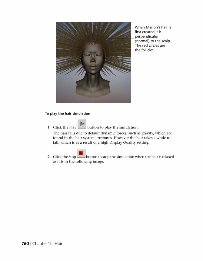
To play the hair simulation
1 Click the Play button to play the simulation.
The hair falls due to default dynamic forces, such as gravity, which arefound in the hair system attributes. However the hair takes a while tofall, which is as a result of a high Display Quality setting.
2 Click the Stop button to stop the simulation when the hair is relaxedas it is in the following image.
760 | Chapter 15 Hair
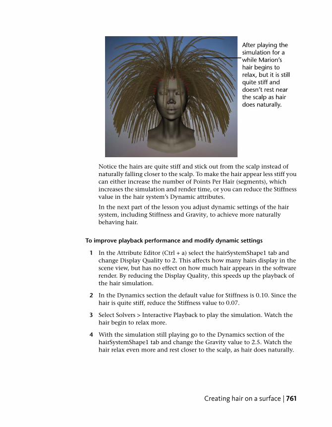
Notice the hairs are quite stiff and stick out from the scalp instead ofnaturally falling closer to the scalp. To make the hair appear less stiff youcan either increase the number of Points Per Hair (segments), whichincreases the simulation and render time, or you can reduce the Stiffnessvalue in the hair system’s Dynamic attributes.
In the next part of the lesson you adjust dynamic settings of the hairsystem, including Stiffness and Gravity, to achieve more naturallybehaving hair.
To improve playback performance and modify dynamic settings
1 In the Attribute Editor (Ctrl + a) select the hairSystemShape1 tab andchange Display Quality to 2. This affects how many hairs display in thescene view, but has no effect on how much hair appears in the softwarerender. By reducing the Display Quality, this speeds up the playback ofthe hair simulation.
2 In the Dynamics section the default value for Stiffness is 0.10. Since thehair is quite stiff, reduce the Stiffness value to 0.07.
3 Select Solvers > Interactive Playback to play the simulation. Watch thehair begin to relax more.
4 With the simulation still playing go to the Dynamics section of thehairSystemShape1 tab and change the Gravity value to 2.5. Watch thehair relax even more and rest closer to the scalp, as hair does naturally.
Creating hair on a surface | 761
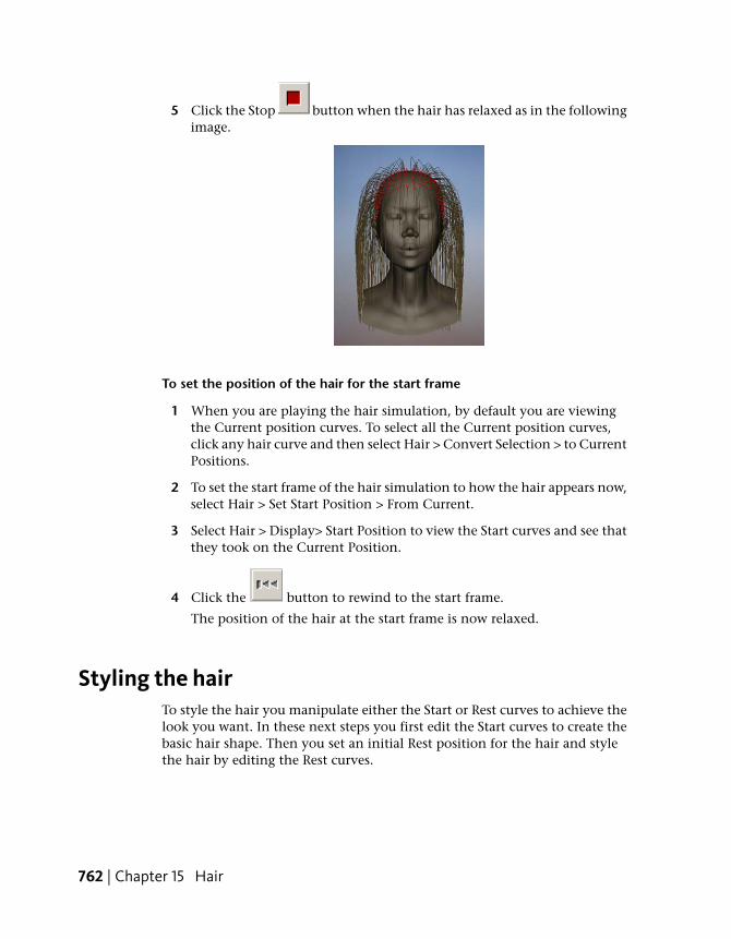
5 Click the Stop button when the hair has relaxed as in the followingimage.
To set the position of the hair for the start frame
1 When you are playing the hair simulation, by default you are viewingthe Current position curves. To select all the Current position curves,click any hair curve and then select Hair > Convert Selection > to CurrentPositions.
2 To set the start frame of the hair simulation to how the hair appears now,select Hair > Set Start Position > From Current.
3 Select Hair > Display> Start Position to view the Start curves and see thatthey took on the Current Position.
4 Click the button to rewind to the start frame.
The position of the hair at the start frame is now relaxed.
Styling the hairTo style the hair you manipulate either the Start or Rest curves to achieve thelook you want. In these next steps you first edit the Start curves to create thebasic hair shape. Then you set an initial Rest position for the hair and stylethe hair by editing the Rest curves.
762 | Chapter 15 Hair

To edit the Start curves to create the basic hair shape
1 Display the Start curves. (Hair > Display> Start Position.
2 Tumble the camera so you’re looking at the side of Marion’s head.
3 To select the Start curves on the front half of Marion’s face, do thefollowing:
■ On the Status Line, click the Object Selection Mask button andchoose All Objects Off from the drop-down menu that appears.
■ On the Status Line, click to highlight the icon to restrict theselection to curves.
■ Drag around the front half of Marion’s head to select the Start curvesas shown in the following image.
4 Now tumble the camera so Marion is again facing you.
5 To trim the Start curves in the front, do the following:
■ Select Hair > Modify Curves > Lock Length. This allows you tomanipulate the curve while maintaining the curve’s hull length.
■ Click the in the Status Line to display the curves’ CVs.
■ Using the Lasso Tool , select CVs in an inverted U-shape aroundthe front of Marion’s face, as shown in the following image.
Styling the hair | 763

■ Press Delete to remove the selected CVs.
6 To curl under the ends of all the Start curves, do the following:
■ Click the button to display the curves and then drag aroundMarion’s head to select all the Start curves.
■ Click the button to display CVs and then, using the Select Tool,select the CVs in the bottom half of all the curves.
■ Select Hair > Modify Curves > Bend .
■ In the Bend Curves Options window, set Bend Amount to 0.5 andTwist to 1.0 and then click Bend Curves.
764 | Chapter 15 Hair

The selected CVs are bent under towards Marion’s neck. To fix any unrulyhairs, you could select them and then select Hair > Modify Curves>Smooth.
7 Click the button to display the curves.
8 Change the display to include the Start curves and the Current Position.(Hair > Display> Current and Start)
9 Click the Play button to play the hair simulation.
Even though you styled the Start curves, notice how they fall straightand lose the bend at the end. Start curves only define the position of thehair at the Start frame of the simulation; once the simulation is startedthe Start curves are affected by the dynamic forces applied to the hairsystem. To “hairspray” a hairstyle, you need to style Rest curves and adjustdynamic hair system settings. In the next steps you create Rest curvesfrom the Start curves.
10 Click the Stop button to stop the simulation.
To create and modify the Rest curves to achieve a hairstyle
1 To create Rest curves from the shaped Start curves, do the following:
■ Select Hair > Display > Start Position
Styling the hair | 765

■ Using the Select Tool , drag to select all the Start curves andthen select Hair > Set Rest Position> From Start.
2 To see the new Rest curves, select Hair > Display> Current and Rest.
3 Select all the hair curves and then click the Play button to play thesimulation. Watch how the Current position hairs flop down becausethe Gravity value is quite high (2.5).
4 To see what the hair would look like without any gravity, go to theDynamics section in the hairSystemShape1 tab and change the Gravityvalue to 0.
Watch the hair try to achieve the Rest position.
5 After the hair reaches the Rest position, change the Gravity value backto 1.0.
6 As the hair starts to fall due to gravity, increase the Stiffness value to 0.2.
If some Rest curves won’t relax and stabilize, increase Length Flex andIterations in the hairSystemShape1 tab.
7 Once the hair stabilizes, click the Stop button to stop the simulation.
8 You can further “hairspray” the curled ends of the Rest curves using theStiffness Scale attribute. The curve in the Stiffness Scale graph illustratesthe amount of stiffness applied along the hair curve from root (left sideof the graph) to tip (right side of the graph). Go to the Dynamics sectionin the hairSystemShape1 tab and change the Stiffness Scale attribute asshown in the following image. These changes add more stiffness to theend of the hair, which will hold the bend more firmly.
9 Play the simulation to see the effect of the changes to Stiffness Scale.
766 | Chapter 15 Hair

10 Stop the simulation once the hair relaxes as in the following image.
11 To reset the Start curves from the simulation, select Hair > Set StartPosition> From Current.
12 Click the button to rewind to the beginning of the simulation.
Setting up hair collisionsBefore trimming Marion’s hair you may have noticed that some hairsintersected her face. As well hairs currently intersect the lower part of herneck. To fix this you set up hair collisions. You can set hair to collide withitself, other objects or the ground (grid). In the next steps you use collisionconstraints to prevent the hair from intersecting with Marion’s head and neck.
Setting up hair collisions | 767

To make Marion’s hair collide with her head and neck
1 In the panel, select Show > Locators so you can see collision constraints,which are locators, when you create them.
2 To create the collision constraint for Marion’s head, do the following:
■ Select Hair > Display > Start Position.
■ Using the Select Tool, drag around all the hair curves and select Hair> Convert Selection > To Start Curves.
■ Select Hair > Create Constraint > Collide Sphere.
■ Using the Scale Tool, resize the sphere so it expands beyond Marion’shead and you can see it.
■ Using the Move Tool, move the sphere up the Y-axis so the top of thesphere is aligned with the top of Marion’s head.
■ Using the Scale Tool again, resize the sphere so it matches the basicshape of Marion’s head. First try scaling in the X direction to adjustthe width of the sphere from ear to ear. Then tumble the camera tosee the side of Marion’s head and scale in the Z direction to adjustthe sphere width from the back of Marion’s head to her nose. Youmay also need to move the sphere to tweak its size and position, asshown in the images below.
768 | Chapter 15 Hair

3 To create the collision constraint for Marion’s upper torso, do thefollowing:
■ Using the Select Tool, drag around the hair curves and select Hair >Convert Selection > To Start Curves.
■ Select Hair > Create Constraint > Collide Sphere.
■ Using the Scale Tool, resize the sphere so it extends beyond Marion’sneck and you can see it.
■ Using the Move Tool, move the sphere down the Y-axis so the top ofthe sphere is aligned with the top of Marion’s torso.
■ Using the Scale Tool again, resize the sphere so it matches the basicdimensions of Marion’s upper torso. First try scaling in the X directionto adjust the width of the sphere from shoulder to shoulder. Thentumble the camera to see the side of Marion’s head and scale in theZ direction to adjust the sphere width from the back of Marion’s torsoto the front of it. You may also need to move the sphere to tweak itssize and position, as shown in the images below.
Setting up hair collisions | 769

4 Select Hair > Display> Current Position.
5 Click the button to rewind to the start frame and play thesimulation.
Watch how the hair collides with the collision constraints you created.The hair at the front now rests on the torso and the hair at the back curlsunder the torso, instead of intersecting it like it did before the collisionswere set.
6 Stop the simulation when the hair is relaxed. Should the hair be unrulyand not relax, you may need to increase the Stiffness or the Iterations inthe Dynamics section of the hairSystemShape1 tab of the Attribute Editor.
7 Select the hair, then select Hair > Set Start Position > From Current sothe hair respects the collisions at the start frame of the simulation.
770 | Chapter 15 Hair

8 Select Show > Locators to turn them off, which hides the collisionconstraints.
Rendering the hairWhen you modify hair attributes, many of these changes are not visible inthe scene view; the Paint Effects hair must be rendered in the Maya Softwarerenderer. In the next steps you render Marion’s hair as it is now, which allowsyou to see what aspects of the hair need work to make it look more realistic.Before rendering, be sure to set the appropriate Render Settings.
To render Paint Effects hair using the Maya Software renderer
1 Modify the Render Settings for Paint Effects.
■ Click the Render Settings button on the Status Line. The RenderSettings window appears.
■ Select Maya Software from the Render using drop-down list.
■ In the Maya Software tab, go to the Paint Effects Rendering Optionssection and turn on Oversample and Oversample post filter. Thesehelp achieve a better look for the Paint Effects rendering. The optionEnable stroke rendering is already on by default.
■ Click Close to close the Render Settings window.
2 Before rendering be sure to display the hair system’s Current Position(Hair > Display > Current Position).
3 Click the Render Current Frame button on the Status Line.
The hair model is rendered and should look something like the imagebelow.
Rendering the hair | 771

Modifying hair attributesYou can modify the hair as a whole by modifying the hair system attributes.You can modify the look of individual hairs or clumps of hair by editing theirfollicle attributes. In the next steps, you modify various hair system attributesto make Marion’s hair look fuller and more realistic. Then you add curl toMarion’s hair.
To modify the thickness of the hair all over
1 To select the hair system, drag around the hair curves and select Hair >Convert Selection > to Hair Systems.
2 Go to the Clump and Hair Shape section in the hairSystemShape1 tab ofthe Attribute Editor and adjust the following:
■ Hairs Per Clump to 30, which controls the number of hairs per curve(hair clump). Increasing the number of Hairs Per Clump increases therendering time.
■ Sub Segments to 2, which adds this many points betweensegments/points and helps to smooth the hair curves.
■ Thinning to 0.5, which controls how much the hair thins out fromroot to tip.
■ Clump Width to 0.3, which controls the width of the hair clump fromroot to tip. To further modify the hair clump width, you could adjustthe Clump Width Scale attribute, which allows you to vary the widthalong the hair from root to tip.
772 | Chapter 15 Hair
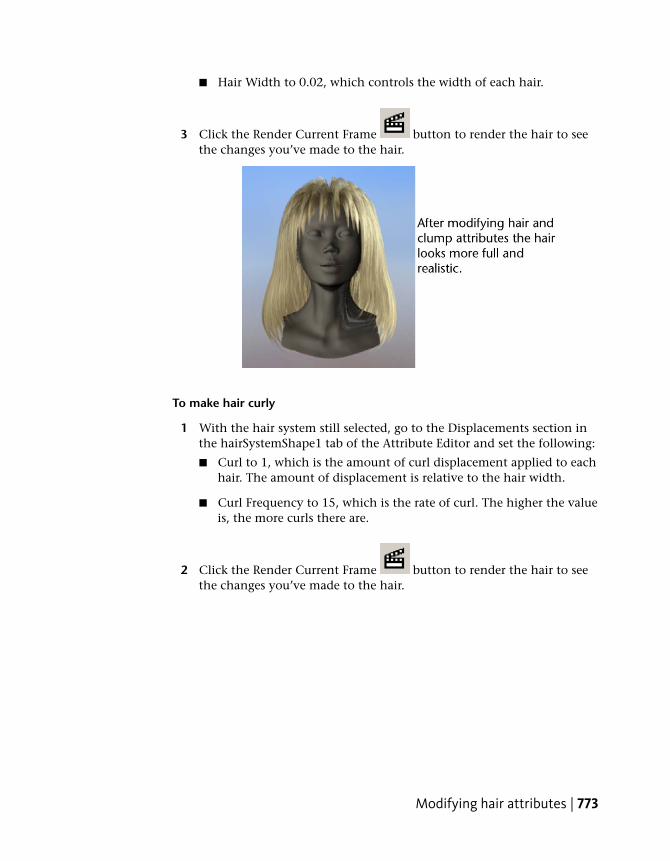
■ Hair Width to 0.02, which controls the width of each hair.
3 Click the Render Current Frame button to render the hair to seethe changes you’ve made to the hair.
To make hair curly
1 With the hair system still selected, go to the Displacements section inthe hairSystemShape1 tab of the Attribute Editor and set the following:
■ Curl to 1, which is the amount of curl displacement applied to eachhair. The amount of displacement is relative to the hair width.
■ Curl Frequency to 15, which is the rate of curl. The higher the valueis, the more curls there are.
2 Click the Render Current Frame button to render the hair to seethe changes you’ve made to the hair.
Modifying hair attributes | 773

Setting up shadowing on hairHair, by default, is translucent so you need to set up self shadowing, otherwisehair appears glowing, like nylon. The darker the hair color is, the moreimportant the specular color and highlights become.
There are three directional lights in this scene. In the software render you didin the previous steps, Marion’s hair appears blond and glowing, even thoughthe default hair color is dark brown, as in the scene view. This apparent haircolor discrepancy occurs because:
■ hair is by default translucent (like a glass tube)
■ the hair is being lit by all three lights, therefore the intensity of the lightis tripled
■ there are no shadows, so all the hairs are illuminated
In these next steps you set up shadows on all three lights.
To set up shadows and self shadows on hair
1 Select Window > Outliner.
2 In the Outliner menu, select Show > Objects > Lights.
3 Select one of the three directional lights.
4 In the light’s Attribute Editor, go to the Shadows section and in the DepthMap Shadow Attributes subsection, turn on Use Depth Map Shadows.
774 | Chapter 15 Hair

Normally you would increase the Filter Size to blur the light in the hairfor realism, and increase the Bias, which sets how far the light filtersthrough the hair. These attributes were set for you in the scene.
5 Repeat steps 3 and 4 for the other two directional lights.
6 Render the hair to see the changes.
The shadows on the hair are hard and there is very little specularity. Youfix this in the next steps.
To create specular highlights on hair
1 To select the hair system, drag around the hair curves and select Hair >Convert Selection > to Hair Systems.
2 Go to the Shading section in the hairSystemShape1 tab of the AttributeEditor and set the following:
■ Click the Specular Color box and set the values as shown in the imagebelow.
■ Increase Specular Power to 15.
3 Render the hair to see the changes. The hair looks much more naturalnow.
Setting up shadowing on hair | 775
Beyond the lessonIn this lesson you learned how to:
■ Create dynamic hair on a surface.You can add hair to a NURBS or polygonal surface by creating or paintingthe hair. For polygons, UVs should be non-overlapping and fit between 0and 1. Automatic mapping is a quick way to achieve this (seeAutomaticUV mapping in the Mapping UVs guide). For more information, seeCreating hair in the Hair guide.
Before creating hair, you should determine which renderer you’ll be usingas this will affect what type of hair output you select: NURBS curves orPaint Effects, or both.
■ Interact with the dynamic playback.While using interactive playback you can modify the hair and see the hairreact to dynamic forces. For more information, see Play a hair simulationin the Hair guide.
■ Model hair curves.Style hair by transforming hair curves and using Lock Length to maintainthe length between CVs on a curve. You can also use Fields to style hairand then add constraints to hold hair in position. For more information,see Styling hair and modifying the hair look and behavior in the Hairguide.
■ Modify hair system and follicle attributes.You can change the look (color, curl, etc.) of the overall hair by modifyingattributes in the hairSystemShape node. But individual follicle attributescan be modified in the follicleShape node, which override or blend withthe hair system attributes. For more information, see the following topicsin the online help: Hair system attributes (hairSystemShape in the Hairguide), Follicle attributes (follicleShape in the Hair guide) and Set up hairshading in the Hair guide.
■ Render the hair.Paint Effects hair can be rendered using the Maya Software renderer. Youcan also convert Paint Effects hair to polygons and render in anotherrenderer, such as mental ray. Or you can output just the dynamic curvesto an external renderer, such as Renderman. For more information, seeRendering scenes with hair in the Hair guide.
776 | Chapter 15 Hair

You can also create non-hair models and effects with Hair. Any NURBS curvecan be made into a dynamic hair curve. In addition to creating long hair andhairstyles you can use hair curves to create:
■ ropes and chains (dynamic curves)
■ a fish (wire deformer)
■ a fishing line (single hair with expressions)
■ an octopus (select hair curves and create a lofted surface)
■ a paint brush painting on canvas, bristles colliding with the surface (hairsimulates paint brush bristles, Fluid emitters on the canvas controlled byexpressions)
In addition you can assign a Paint Effects brush to a hair system as shown inthe image below.
Lesson 2: Creating a dynamic non-hair simulation
IntroductionUsing Maya Hair, you can create dynamic non-hair models and effects. Youcan make NURBS curves dynamic, or you can use a hair system to create a
Lesson 2: Creating a dynamic non-hair simulation | 777

non-hair simulation, such as chains or ropes. In this lesson, you create a hairsystem to simulate a beaded curtain. To make the hairs look like beads, youassign a Paint Effects brush to the hair. Then you modify the hair attributesand set constraints so the hair behaves like a beaded curtain hanging from acurtain rod.
In this lesson, you learn how to:
■ Make hair collide with an object
■ Assign a Paint Effects brush to hair
■ Set up hair constraints
Lesson setupIn this lesson, you work with a new empty scene and change the playbackrange.
1 Select File > New Scene.
2 In the Time Slider change both the End Time value and Playback EndTime value to 300.
Setting up the curtain sceneIn these steps you model a 2D curtain rod from a plane and attach hair to it.Then you add and keyframe a sphere in the scene to later be used as a collisionobject.
778 | Chapter 15 Hair

To create the curtain using Hair
1 To create a NURBS plane, select Create > NURBS Primitives > Plane, thenclick-drag in the scene to create a plane.
(If you have previously shut off the interactive primitive creation option,simply click once in the scene to create the primitive at the origin.)
2 Using the Scale Tool , resize the plane in the X direction as shownin the image below.
3 With the plane selected, select Hair > Create Hair > , set the followingoptions and then click Create Hairs:
■ Output to NURBS Curves
■ U Count to 20, V count to 1
■ Passive fill to 0
■ Randomization to 0
■ Points per hair to 12
■ Length to 10
■ Turn off the options Create Rest Curves, Edge Bounded and Equalize
Hair is created and attached to the plane.
Setting up the curtain scene | 779

4 Select the plane and, using the Rotate Tool , rotate the plane sothe hair appears to be on the underside of the plane. Then, using the
Move Tool , move the plane up the Y axis so the bottom of thehair just touches the ground plane, as shown in the following image.(Ensure you do not select the hair when selecting the plane.)
5 Create a directional light (Create > Lights > Directional Light) and do thefollowing:
■ Move the light above and to the left of the curtain.
■ Rotate the light so it aims at the curtain.
■ In the light’s Attribute Editor (ctrl + a) go to the Directional LightAttributes section and change the Intensity value to 1.5.
6 Create a NURBS sphere (Create > NURBS Primitives > Sphere) and moveit along the Z-axis so it’s in front of the curtain.
780 | Chapter 15 Hair

7 To set the start keyframe for the sphere, do the following:
■ Go to frame 1 on the Time Slider.
■ In the Channel Box, drag to select the Translate X, Y, and Z channels.
■ Right-click the channels and select Key Selected.
8 To set the keyframe for the sphere and move it through the curtain, asin the image below, do the following:
■ Go to frame 100 in the Time Slider.
■ Move the sphere in the Z direction as shown in the image below.
■ In the Channel Box, select the Translate Z channel.
■ Right-click the channel and select Key Selected.
9 Rewind the Time Slider to 0 and play the animation.
The sphere passes through the curtain as though the curtain weren’tthere. In the next steps you set the sphere as a collision object with thehair.
Setting up the curtain scene | 781
Making the hair collide with another objectTo have hair interact with a surface, you must set the hair to collide with thesurface. A collision object can be a NURBS or polygonal surface. In the nextpart of the lesson you set the curtain to collide with the sphere and then playthe simulation.
To enhance the curtain for collisions
1 To select the hair system, drag around the hair curves and then selectHair > Convert Selection > To Hair Systems.
2 In the hairSystemShape1 tab of the Attribute Editor, set the hair systemattributes as follows:
■ In the Clump and Hair Shape section, set Clump Width to 0.
■ In the Dynamics section, set Stiffness to 0.
To make the hair collide with the sphere
1 Select the hair system and the sphere (drag around the hair curves andsphere).
2 Select Hair > Make Collide.
3 Play the simulation.
Now the sphere collides with the curtain, pushing the strands of hairaside as it passes through.
Assigning a Paint Effects brush to the hairYou can assign a Paint Effects brush to a hair system to achieve a variety ofeffects. In these next steps you apply the red beads brush to the hair systemto create the beaded curtain. Then you modify the brush and hair systemsettings to achieve the desired look.
To turn the hair curtain into a beaded curtain
1 To select the hair system, drag around the hair curves and select Hair >Convert Selection > To Hair Systems.
2 Open the Visor (Window > General Editors > Visor).
3 Go to the glass folder and select the beadsRed.mel brush.
782 | Chapter 15 Hair
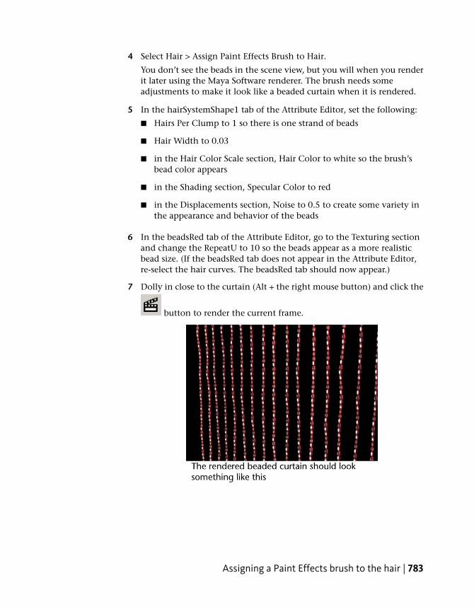
4 Select Hair > Assign Paint Effects Brush to Hair.
You don’t see the beads in the scene view, but you will when you renderit later using the Maya Software renderer. The brush needs someadjustments to make it look like a beaded curtain when it is rendered.
5 In the hairSystemShape1 tab of the Attribute Editor, set the following:
■ Hairs Per Clump to 1 so there is one strand of beads
■ Hair Width to 0.03
■ in the Hair Color Scale section, Hair Color to white so the brush’sbead color appears
■ in the Shading section, Specular Color to red
■ in the Displacements section, Noise to 0.5 to create some variety inthe appearance and behavior of the beads
6 In the beadsRed tab of the Attribute Editor, go to the Texturing sectionand change the RepeatU to 10 so the beads appear as a more realisticbead size. (If the beadsRed tab does not appear in the Attribute Editor,re-select the hair curves. The beadsRed tab should now appear.)
7 Dolly in close to the curtain (Alt + the right mouse button) and click the
button to render the current frame.
Assigning a Paint Effects brush to the hair | 783
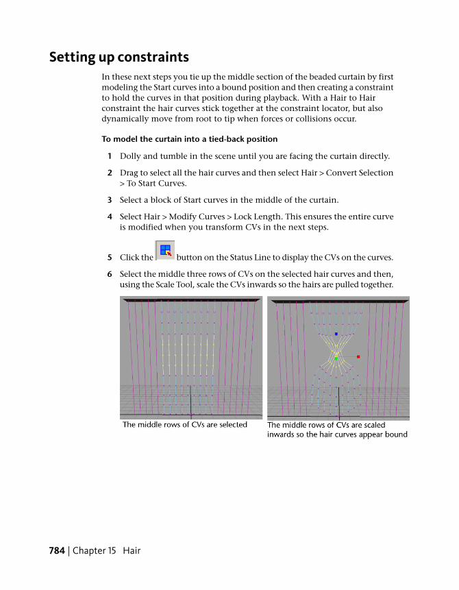
Setting up constraintsIn these next steps you tie up the middle section of the beaded curtain by firstmodeling the Start curves into a bound position and then creating a constraintto hold the curves in that position during playback. With a Hair to Hairconstraint the hair curves stick together at the constraint locator, but alsodynamically move from root to tip when forces or collisions occur.
To model the curtain into a tied-back position
1 Dolly and tumble in the scene until you are facing the curtain directly.
2 Drag to select all the hair curves and then select Hair > Convert Selection> To Start Curves.
3 Select a block of Start curves in the middle of the curtain.
4 Select Hair > Modify Curves > Lock Length. This ensures the entire curveis modified when you transform CVs in the next steps.
5 Click the button on the Status Line to display the CVs on the curves.
6 Select the middle three rows of CVs on the selected hair curves and then,using the Scale Tool, scale the CVs inwards so the hairs are pulled together.
784 | Chapter 15 Hair

To constrain the curtain in the tied-back position
1 Click the button on the Status Line to display the Start curves (notthe CVs).
2 With the bound hair curves still selected, select Hair > Create Constraint> Hair to Hair.
A constraint locator is created and connected to the selected curves.
3 In the hairConstraintShape tab in the Attribute Editor, set the constraintattributes as follows:
■ Stiffness to 0.5 (default)
■ Glue Strength to 1.0 (default)
■ Point Method to Nearest (default) (Since the constraint locator iscreated in the middle of the bound hair, the locator is “nearest” thebound area to be constrained.)
4 Change the hair display to the Current Position (Hair > Display > CurrentPosition).
5 Rewind to the start frame and play the simulation.
When the sphere passes through the bound curtain it collides with allthe bound hairs.
The bound part of the curtain relaxes within the first several frames, butin the next steps you reset the position of those Start curves so they lookmore natural at the beginning of the simulation.
Setting up constraints | 785

To reset the Start position
1 Display the Start curves and the Current Position (Hair > Display > Currentand Start).
2 Rewind to the start frame and play the simulation.
3 Stop the simulation as soon as the curves relax below the constraint, butbefore the collision occurs.
4 Select the bound Start curves (these are the bound curves that are notblue) and then select Hair > Set Start Position > From Current.
You may have to repeat steps 2 to 4 a few times until you are happy withthe look of the bound curtains at the beginning of the simulation.
Rendering the curtain sceneIn these next steps you render the curtain, which is Paint Effects hair, in theMaya Software renderer.
To render the Paint Effects hair using the Maya Software renderer
1 To modify the Render Settings for Paint Effects do the following:
■ Click the Render Settings button on the Status Line. The RenderSettings window appears.
786 | Chapter 15 Hair
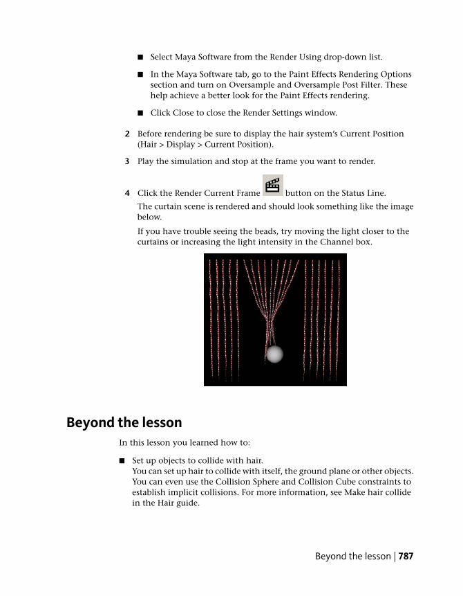
■ Select Maya Software from the Render Using drop-down list.
■ In the Maya Software tab, go to the Paint Effects Rendering Optionssection and turn on Oversample and Oversample Post Filter. Thesehelp achieve a better look for the Paint Effects rendering.
■ Click Close to close the Render Settings window.
2 Before rendering be sure to display the hair system’s Current Position(Hair > Display > Current Position).
3 Play the simulation and stop at the frame you want to render.
4 Click the Render Current Frame button on the Status Line.
The curtain scene is rendered and should look something like the imagebelow.
If you have trouble seeing the beads, try moving the light closer to thecurtains or increasing the light intensity in the Channel box.
Beyond the lessonIn this lesson you learned how to:
■ Set up objects to collide with hair.You can set up hair to collide with itself, the ground plane or other objects.You can even use the Collision Sphere and Collision Cube constraints toestablish implicit collisions. For more information, see Make hair collidein the Hair guide.
Beyond the lesson | 787

■ Assign a Paint Effects brush to a hair system.This is useful for creating a variety of effects, such as vines or ivy for hair.The hair output can be Paint Effects or NURBS curves. For moreinformation, see Assign a Paint Effects brush to Hair in the Hair guide.
■ Create constraints on hair curves.Use hair constraints to hold hair in position for a hairstyle, such as aponytail or a clasp. You can even use hair constraints for more realistichair behavior, such as using the Transform constraint to hold the hair tothe head. For more information, see Set up hair constraints in the Hairguide.
788 | Chapter 15 Hair
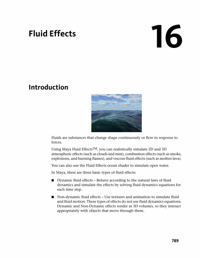
Fluid Effects
Introduction
Fluids are substances that change shape continuously or flow in response toforces.
Using Maya Fluid EffectsTM, you can realistically simulate 2D and 3Datmospheric effects (such as clouds and mist), combustion effects (such as smoke,explosions, and burning flames), and viscous fluid effects (such as molten lava).
You can also use the Fluid Effects ocean shader to simulate open water.
In Maya, there are three basic types of fluid effects:
■ Dynamic fluid effects – Behave according to the natural laws of fluiddynamics and simulate the effects by solving fluid dynamics equations foreach time step.
■ Non-dynamic fluid effects – Use textures and animation to simulate fluidand fluid motion. These types of effects do not use fluid dynamics equations.Dynamic and Non-Dynamic effects render as 3D volumes, so they interactappropriately with objects that move through them.
16
789
■ Open water fluid effects – Use shaders to create realistic wave motion onlarge bodies of water.
This chapter includes the following lessons, which introduce you to somebasic Fluid Effects concepts:
■ Lesson 1 Creating a dynamic 2D fluid effect: Introduction on page 791
■ Lesson 2 Creating a non-dynamic 3D fluid effect: Introduction on page801
■ Lesson 3 Creating a dynamic 3D effect: Introduction on page 810
■ Lesson 4 Creating an ocean effect: Introduction on page 819
Preparing for the lessonsTo ensure the lessons work as described, do these steps before beginning:
1 Create a new scene.
2 If you have not already done so, copy the GettingStarted folder fromits installation location to your projects directory. Then, set theGettingStarted directory as your Maya project. For more information,see Copying and setting the Maya project on page 25 in the GettingStarted with Maya guide.
3 Select the Dynamics menu set.
Unless otherwise noted, the directions in this chapter for making menuselections assume you’ve already selected the Dynamics menu set.
4 Switch to shaded display mode for a hardware render view of the fluidsimulations (Shading > Smooth Shade All on the view menu bar).
5 In the Time and Range slider, set the start frame to 1 and end frame to200.
6 Before you perform the lessons in this chapter, ensure that the InteractiveCreation option for primitives is turned off by selecting Create > PolygonPrimitives > Interactive Creation and Create > NURBS Primitives >Interactive Creation. That is, ensure that a check mark does not appearbeside either of these menu items.
790 | Chapter 16 Fluid Effects

7 Make sure you understand the basic usage of the animation playbackcontrols. See the chapter entitled “Animation” in Getting Started withMaya or refer to the Maya Help.
Lesson 1: Creating a dynamic 2D fluid effect
Introduction
Fluid dynamics is a branch of physics that uses mathematical equations todescribe how things flow.
In Fluid Effects, dynamic fluid effects simulate fluid motion by solving fluiddynamics equations at each time step. You can texture dynamic fluids, havethem collide with and move geometry, affect soft body geometry, and interactwith particles.
Non-dynamic fluid effects do not use fluid dynamics equations to simulatefluid behavior. You create the look of a non-dynamic fluid using textures, andyou create fluid motion by animating (keyframing) texture attributes. BecauseMaya doesn’t solve the equations, rendering this type of fluid is much quickerthan rendering a dynamic fluid.
In this lesson, you create a simple two-dimensional dynamic fluid. You learnhow to:
■ Create a fluid using fluid emitters
■ Modify the dynamic behavior of the fluid by applying forces to it andchanging the effect the boundary has on the fluid
■ Change the color of the fluid
■ Collide the fluid into an object
In the next lesson, you’ll create a non-dynamic fluid effect.
Lesson 1: Creating a dynamic 2D fluid effect | 791
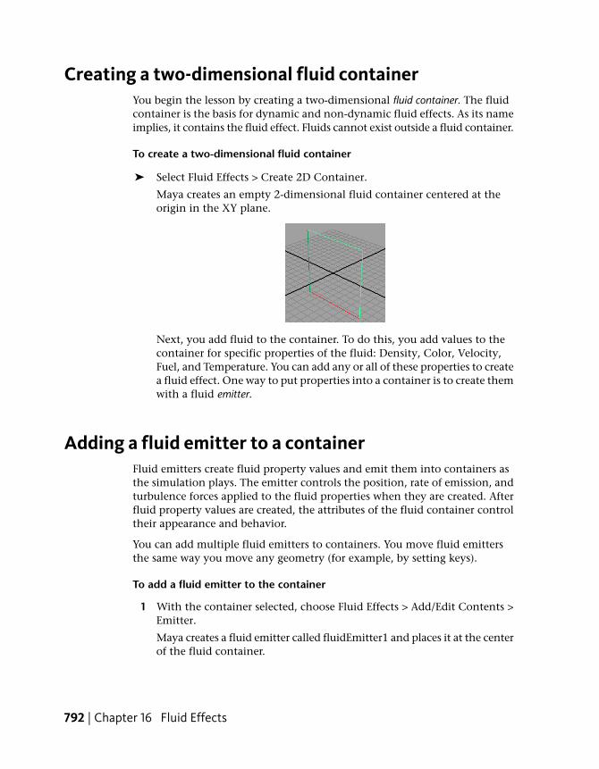
Creating a two-dimensional fluid containerYou begin the lesson by creating a two-dimensional fluid container. The fluidcontainer is the basis for dynamic and non-dynamic fluid effects. As its nameimplies, it contains the fluid effect. Fluids cannot exist outside a fluid container.
To create a two-dimensional fluid container
➤ Select Fluid Effects > Create 2D Container.
Maya creates an empty 2-dimensional fluid container centered at theorigin in the XY plane.
Next, you add fluid to the container. To do this, you add values to thecontainer for specific properties of the fluid: Density, Color, Velocity,Fuel, and Temperature. You can add any or all of these properties to createa fluid effect. One way to put properties into a container is to create themwith a fluid emitter.
Adding a fluid emitter to a containerFluid emitters create fluid property values and emit them into containers asthe simulation plays. The emitter controls the position, rate of emission, andturbulence forces applied to the fluid properties when they are created. Afterfluid property values are created, the attributes of the fluid container controltheir appearance and behavior.
You can add multiple fluid emitters to containers. You move fluid emittersthe same way you move any geometry (for example, by setting keys).
To add a fluid emitter to the container
1 With the container selected, choose Fluid Effects > Add/Edit Contents >Emitter.
Maya creates a fluid emitter called fluidEmitter1 and places it at the centerof the fluid container.
792 | Chapter 16 Fluid Effects

TIP You can create a fluid container with a fluid emitter in one step usingFluid Effects > Create 2D Container with Emitter.
2 Play the simulation using the playback controls at the bottom of theMaya window.
The fluid emitter creates Density values and emits them into thecontainer.
The white in the container represents Density. Density is the substanceof the fluid and the visible fluid property. Where the Density values arehighest, the Density appears more opaque.
Notice that the Density rises to the top of the container and moves alongthe boundary of the container, eventually flowing down the sides. Forcesbuilt into the container are acting on the Density values, causing themto change. The fluid collides with the boundaries rather than penetratingthem.
Adding a fluid emitter to a container | 793
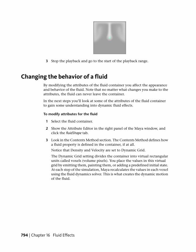
3 Stop the playback and go to the start of the playback range.
Changing the behavior of a fluidBy modifying the attributes of the fluid container you affect the appearanceand behavior of the fluid. Note that no matter what changes you make to theattributes, the fluid can never leave the container.
In the next steps you’ll look at some of the attributes of the fluid containerto gain some understanding into dynamic fluid effects.
To modify attributes for the fluid
1 Select the fluid container.
2 Show the Attribute Editor in the right panel of the Maya window, andclick the fluidShape tab.
3 Look in the Contents Method section. The Contents Method defines howa fluid property is defined in the container, if at all.
Notice that Density and Velocity are set to Dynamic Grid.
The Dynamic Grid setting divides the container into virtual rectangularunits called voxels (volume pixels). You place the values in this virtualgrid by emitting them, painting them, or adding a predefined initial state.At each step of the simulation, Maya recalculates the values in each voxelusing the fluid dynamics solver. This is what creates the dynamic motionof the fluid.
794 | Chapter 16 Fluid Effects

TIP You can display Density values for the virtual grid by changing NumericDisplay to Density in the Display section of the fluid Attribute Editor. Set theshading mode to Wireframe.
For dynamic fluid simulations, Density must be set to Dynamic Grid.Also, Velocity cannot be turned Off because velocity moves the propertyvalues around inside the grid.
You look at defining properties as Gradient and Static Grid in the nextlessons.
4 Make the density fall instead of rise by opening the Dynamic Simulationsection of the Attribute Editor and setting the following:
■ Change the Gravity value to -9.8. (Acceleration due to gravity is -9.8m/s2 in the physical world.)
Negative values move the Density down.
5 Play the simulation using the playback controls at the bottom of theMaya window.
6 To add turbulence to the container and give the Density a whirlingcircular motion.
■ Ensure the fluid container is selected if it is not already.
Changing the behavior of a fluid | 795

■ In the Attribute Editor, open the Contents Details section, and thenopen the Turbulence section.
■ Change the Strength value to 1.0.
7 Play the simulation using the playback controls at the bottom of theMaya window.
8 Stop the playback and go to the start of the playback range.
9 Change the effect of the container boundaries on the fluid:
■ In the Container Properties section at the top of the Attribute Editor,set the following options:
■ Boundary X: None
■ Boundary Y: None
10 Play the simulation using the playback controls at the bottom of theMaya window.
Notice that the fluid no longer collides with the sides of the container—itappears to pass through the sides. The fluid behaves as though thecontainer boundaries don’t exist. Note that even though the fluid appearsto pass through the container boundaries, it does not exist outside theboundary. Fluids can only exist inside containers.
11 Change Boundary X and Boundary Y back to Both Sides to restore theboundaries at all sides of the container.
796 | Chapter 16 Fluid Effects

12 Stop the playback and go to the start of the playback range.
Combining colors in a fluidIn the next steps, you’ll add another emitter to the container and make eachemitter create different colored Density. You’ll see how different coloredDensity interacts in the container.
To combine colored fluids in the container
1 Select the fluid container and choose Fluid Effects > Add/Edit Contents> Emitter.
Maya creates a second fluid emitter called fluidEmitter2 and places it atthe center of the fluid container, in the same position as the first emitter.
2 With fluidEmitter2 still selected, select the Move Tool (Hotkey: w) anddrag the emitter to the right of the container, so the emitters no longeroverlap.
Make sure you keep the emitter inside the container and on the planeby dragging only the X and Y manipulators. If you move the emitteroutside the container, it will not emit.
3 Open the Attribute Editor in the right panel of the Maya window, andclick the fluidEmitter2 tab.
4 In the Fluid Attributes section, turn on Emit Fluid Color.
A message appears prompting you to set the fluid’s Color Method toDynamic Grid.
By setting the Color Method to Dynamic Grid, the color values you placein the container grid are recalculated by the fluid dynamics solver andchanged during simulation. This means colors can interact during thesimulation.
Combining colors in a fluid | 797
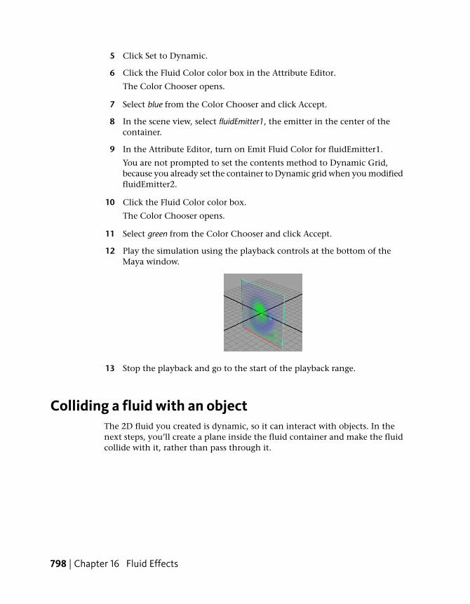
5 Click Set to Dynamic.
6 Click the Fluid Color color box in the Attribute Editor.
The Color Chooser opens.
7 Select blue from the Color Chooser and click Accept.
8 In the scene view, select fluidEmitter1, the emitter in the center of thecontainer.
9 In the Attribute Editor, turn on Emit Fluid Color for fluidEmitter1.
You are not prompted to set the contents method to Dynamic Grid,because you already set the container to Dynamic grid when you modifiedfluidEmitter2.
10 Click the Fluid Color color box.
The Color Chooser opens.
11 Select green from the Color Chooser and click Accept.
12 Play the simulation using the playback controls at the bottom of theMaya window.
13 Stop the playback and go to the start of the playback range.
Colliding a fluid with an objectThe 2D fluid you created is dynamic, so it can interact with objects. In thenext steps, you’ll create a plane inside the fluid container and make the fluidcollide with it, rather than pass through it.
798 | Chapter 16 Fluid Effects

To make the fluid collide with a plane
1 Create a polygon plane:
■ Select Create > Polygon Primitives > Plane > . The Polygon PlaneOptions window opens.
■ In the window, select Edit > Reset Settings to reset the plane settingsto the default ones, and then click Create.
2 In the Attribute Editor, click the pPlane1 tab and scale, translate, andmodify the plane as follows:
■ Translate: -2 2 0
■ Rotate Axis: 0 0 40
■ Scale: 10 1 1
3 Select both the plane and the fluid container.
4 Select Fluid Effects > Make Collide. This makes the plane a collision object.
5 Play the simulation using the playback controls at the bottom of theMaya window.
The fluid collides with the plane as it moves through the container. Itdoes not pass through the plane.
Colliding a fluid with an object | 799

Beyond the lessonThis lesson introduced you to some basic concepts of dynamic fluids. Youlearned how to:
■ Create an empty fluid container.
■ Emit fluid properties into the container to create a dynamic fluid effect.
■ Modify forces acting on the fluid container to change the behavior of thecontents of the container (Gravity and Turbulence).
■ Add color to a fluid by emitting color into the container.
■ Make a fluid collide with an object.
The hardware render of the simulation provided you with a fast, realisticrepresentation of the fluid. The final step would be to do a software render.
Although we looked at a 2D fluid, the same concepts apply to 3D fluids. Inthe lessons that follow, you’ll work with 3D fluids and explore methods otherthan fluid emitters for adding contents to a fluid container. You’ll look at thetexturing capabilities that are part of the built-in shader. You’ll also learnabout the Temperature and Fuel fluid properties and how you can use themin your effects.
Beyond this, you can also:
■ Emit fluid from the surface of an object.
■ Give the fluid a hard surface (surface render) for a globby or lava-like effect,rather than the soft, cloud-like surface you saw in this lesson.
■ Cache the fluid simulation for faster playback.
■ Deform an object with the force of a fluid.
For details on these topics, see the Fluid Effects information in the Maya Help.
800 | Chapter 16 Fluid Effects

Lesson 2: Creating a non-dynamic 3D fluid effect
Introduction
In the first lesson, you created a simple 2D dynamic fluid. 3D fluids intrinsicallyrequire extra data to define them, which can make them very complex. Thisextra data can slow a dynamic simulation exponentially because morecalculations (solving) must be performed at every step of the simulation. Fora less memory intensive effect, you could use a 2D fluid (with less data), oryou could create a 3D non-dynamic effect.
In non-dynamic fluid effects, the fluid property values are predefined withinMaya and stay constant over time, which means they don’t have to berecalculated. You create the appearance of the fluid by texturing a special fluidshader that is assigned to the fluid. This shader is built into the fluid for betterperformance. If you want the fluid effect to have motion, you can animate(keyframe) the texture attributes. Because Maya doesn’t solve the fluiddynamics equations, rendering this type of fluid is much quicker thanrendering a dynamic fluid.
In this lesson, you learn the fundamentals of creating non-dynamic fluids bycreating a cloud bank using a 3D non-dynamic fluid. You learn how to:
■ Create a 3D fluid using predefined gradient contents.
■ Texture the contents of the fluid using the built-in fluid shader.
Before beginning the lesson, do the steps in Preparing for the lessons on page790.
Creating a 3D fluid containerCreating a fluid container is the first step in creating a non-dynamic fluideffect.
Lesson 2: Creating a non-dynamic 3D fluid effect | 801

Fluid containers do not need to be uniform in X, Y, and Z. In fact, becauselarger fluids take longer to render, you should make containers only as largein each direction as necessary for the effect. A cloud bank sits above the groundlike a blanket, so the container can be rectangular rather than cubic.
To create a 3D fluid container
1 Select Fluid Effects > Create 3D Container > .
The Create 3D Container Options window opens.
2 Set the container options as follows, then click Apply and Close:
■ X Resolution: 50
■ Y Resolution: 5
■ Z Resolution: 60
■ X Size: 50.0
■ Y Size: 5.0
■ Z Size: 60.0
The resolution is defined in voxels. Higher resolutions produce finerdetail, but increase rendering time. The size of the container is definedin the working units set for Maya. The size of the fluid determines thesize of each voxel.
TIP It’s good practice to make the container’s Resolution and Size proportionalto ensure that the voxels are square making the quality the same along eachaxis.
Maya creates an empty 3-dimensional fluid container centered at theorigin.
Next, you add fluid to the container.
802 | Chapter 16 Fluid Effects
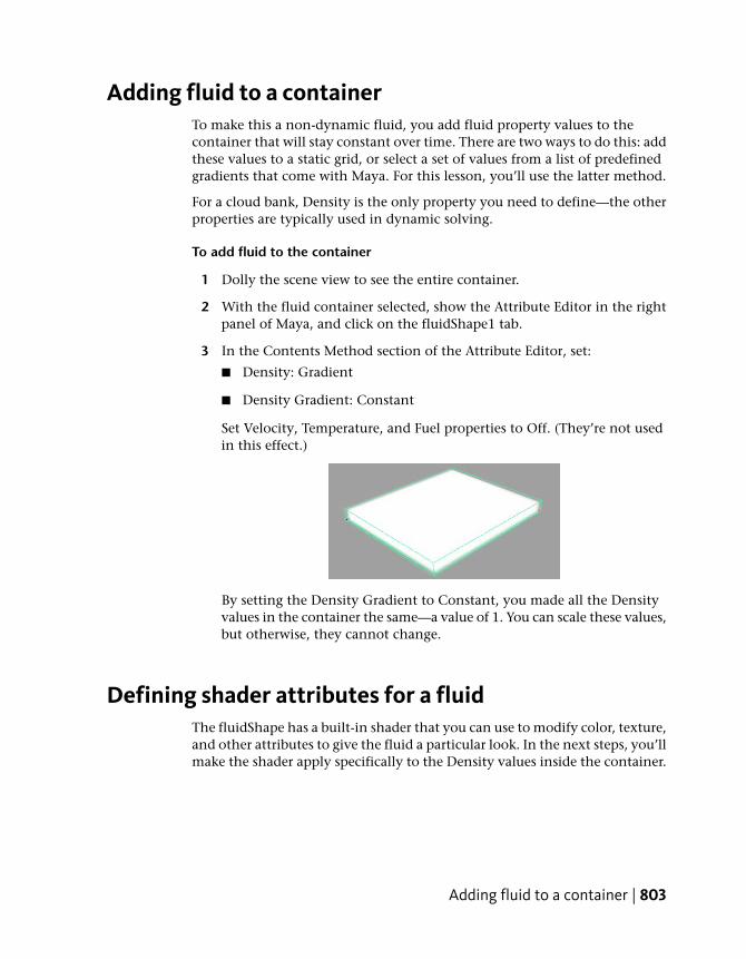
Adding fluid to a containerTo make this a non-dynamic fluid, you add fluid property values to thecontainer that will stay constant over time. There are two ways to do this: addthese values to a static grid, or select a set of values from a list of predefinedgradients that come with Maya. For this lesson, you’ll use the latter method.
For a cloud bank, Density is the only property you need to define—the otherproperties are typically used in dynamic solving.
To add fluid to the container
1 Dolly the scene view to see the entire container.
2 With the fluid container selected, show the Attribute Editor in the rightpanel of Maya, and click on the fluidShape1 tab.
3 In the Contents Method section of the Attribute Editor, set:
■ Density: Gradient
■ Density Gradient: Constant
Set Velocity, Temperature, and Fuel properties to Off. (They’re not usedin this effect.)
By setting the Density Gradient to Constant, you made all the Densityvalues in the container the same—a value of 1. You can scale these values,but otherwise, they cannot change.
Defining shader attributes for a fluidThe fluidShape has a built-in shader that you can use to modify color, texture,and other attributes to give the fluid a particular look. In the next steps, you’llmake the shader apply specifically to the Density values inside the container.
Adding fluid to a container | 803
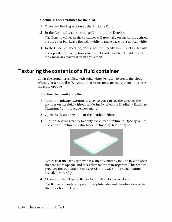
To define shader attributes for the fluid
1 Open the Shading section in the Attribute Editor.
2 In the Color subsection, change Color Input to Density.
The Density values in the container will now take on the colors definedon the color bar. Leave the color white to make the clouds appear white.
3 In the Opacity subsection, check that the Opacity Input is set to Density.
The opacity represents how much the Density will block light. You’lllook more at Opacity later in this lesson.
Texturing the contents of a fluid containerSo far the container is filled with solid white Density. To create the cloudeffect, you texture the Density so that some areas are transparent and someareas are opaque.
To texture the density of a fluid
1 Turn on hardware texturing display so you can see the effect of thetextures on the fluid without rendering by selecting Shading > HardwareTexturing from the scene view menu.
2 Open the Textures section in the Attribute Editor.
3 Turn on Texture Opacity to apply the current texture to Opacity values.The current texture is Perlin Noise, defined by Texture Type.
Notice that the Density now has a slightly blotchy look to it, with areasthat are more opaque and areas that are more transparent. This textureprovides the standard 3D noise used in the 3D Solid Fractal textureincluded with Maya.
4 Change Texture Type to Billow for a fluffy, cloud-like effect.
The Billow texture is computationally intensive and therefore slower thanthe other texture types.
804 | Chapter 16 Fluid Effects
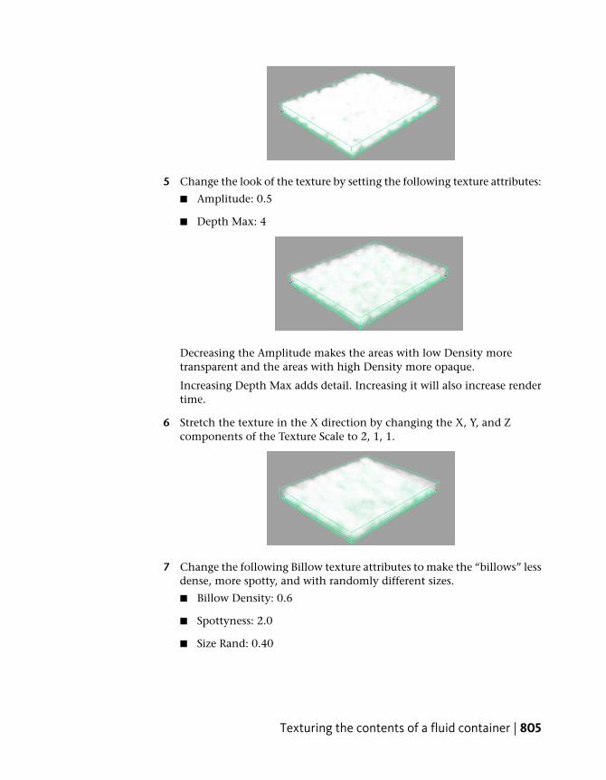
5 Change the look of the texture by setting the following texture attributes:
■ Amplitude: 0.5
■ Depth Max: 4
Decreasing the Amplitude makes the areas with low Density moretransparent and the areas with high Density more opaque.
Increasing Depth Max adds detail. Increasing it will also increase rendertime.
6 Stretch the texture in the X direction by changing the X, Y, and Zcomponents of the Texture Scale to 2, 1, 1.
7 Change the following Billow texture attributes to make the “billows” lessdense, more spotty, and with randomly different sizes.
■ Billow Density: 0.6
■ Spottyness: 2.0
■ Size Rand: 0.40
Texturing the contents of a fluid container | 805
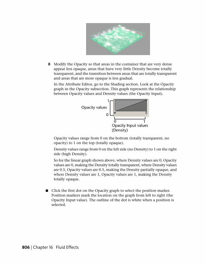
8 Modify the Opacity so that areas in the container that are very denseappear less opaque, areas that have very little Density become totallytransparent, and the transition between areas that are totally transparentand areas that are more opaque is less gradual.
In the Attribute Editor, go to the Shading section. Look at the Opacitygraph in the Opacity subsection. This graph represents the relationshipbetween Opacity values and Density values (the Opacity Input).
Opacity values range from 0 on the bottom (totally transparent, noopacity) to 1 on the top (totally opaque).
Density values range from 0 on the left side (no Density) to 1 on the rightside (high Density).
So for the linear graph shown above, where Density values are 0, Opacityvalues are 0, making the Density totally transparent, where Density valuesare 0.5, Opacity values are 0.5, making the Density partially opaque, andwhere Density values are 1, Opacity values are 1, making the Densitytotally opaque.
■ Click the first dot on the Opacity graph to select the position marker.Position markers mark the location on the graph from left to right (theOpacity Input value). The outline of the dot is white when a position isselected.
806 | Chapter 16 Fluid Effects

■ Change Selected Position to 0.10 to change the position of the marker.
The position marker moves to the right. Now, for Density values between0 and 0.10, the Opacity values will be 0. This means that Density that waspreviously partially transparent will be completely transparent.
The more transparent areas of cloud disappeared, but now the solid areasof cloud are less opaque.
■ Click on the graph to create a new position marker.
■ Change the marker position and value as follows:
■ Selected Position: 0.15
■ Selected Value: 0.30
Texturing the contents of a fluid container | 807

Density values that are greater than 0.15 are now more opaque, and thetransition between areas of total transparency (Opacity 0), and areas wherethe Density becomes more visible (Density 0.15) is less gradual.
Adding self shadowing to texture densityGive the clouds some depth by adding self shadowing. Self shadowing causesthe fluid to cast shadows on itself using a single internal directional light at-1, -1, -1.
To add self shadowing to the texture density
1 In the Attribute Editor, under the fluidShape1 tab, open the Lightingsection.
2 Turn on Self Shadow.
The clouds now have some darker areas on them, giving them somedepth.
3 In the Display section, change Boundary Draw to None to hide thecontainer. This gives you a better idea of how the fluid will look beforeyou render it.
808 | Chapter 16 Fluid Effects
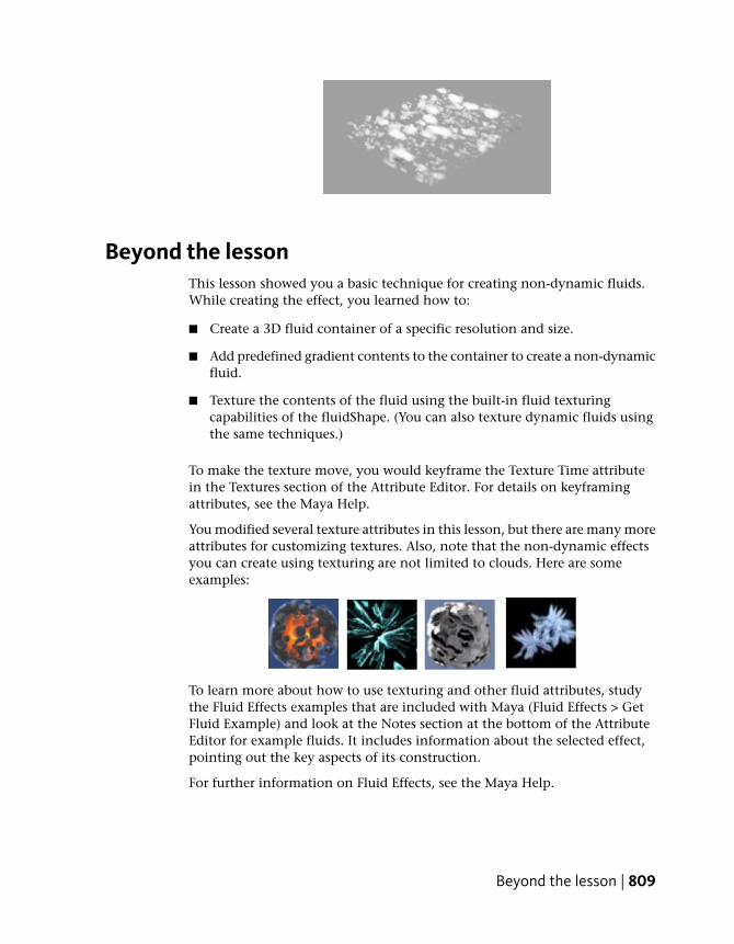
Beyond the lessonThis lesson showed you a basic technique for creating non-dynamic fluids.While creating the effect, you learned how to:
■ Create a 3D fluid container of a specific resolution and size.
■ Add predefined gradient contents to the container to create a non-dynamicfluid.
■ Texture the contents of the fluid using the built-in fluid texturingcapabilities of the fluidShape. (You can also texture dynamic fluids usingthe same techniques.)
To make the texture move, you would keyframe the Texture Time attributein the Textures section of the Attribute Editor. For details on keyframingattributes, see the Maya Help.
You modified several texture attributes in this lesson, but there are many moreattributes for customizing textures. Also, note that the non-dynamic effectsyou can create using texturing are not limited to clouds. Here are someexamples:
To learn more about how to use texturing and other fluid attributes, studythe Fluid Effects examples that are included with Maya (Fluid Effects > GetFluid Example) and look at the Notes section at the bottom of the AttributeEditor for example fluids. It includes information about the selected effect,pointing out the key aspects of its construction.
For further information on Fluid Effects, see the Maya Help.
Beyond the lesson | 809
Lesson 3: Creating a dynamic 3D effect
Introduction
In the real world, gasoline reacts chemically with oxygen at a certaintemperature, creating flames (light, heat) and the gaseous products ofcombustion. Over time, the gasoline burns until it’s totally consumed. Youcan simulate this situation in Fluid Effects using Fuel, Density, and Temperatureproperties.
In this lesson, you create a dynamic explosion effect by filling the bottom ofa container with Fuel and Density, then “igniting” it with Temperature. Youlearn how to:
■ Add property values to a container by painting them.
■ Paint in a 3D container.
■ Use Fuel, Density, and Temperature to create an explosion effect.
Before beginning the lesson, do the steps in Preparing for the lessons on page790.
Creating a 3D container1 Select Fluid Effects > Create 3D Container > .
The Create 3D Container Options window opens.
2 In the window, select Edit > Reset Settings to restore the Resolution andSize settings to the defaults 10 10 10 and 10 10 10, respectively.
The default container size and resolution are adequate to illustrate theconcepts in this lesson.
3 Click Apply and Close.
810 | Chapter 16 Fluid Effects

Maya creates an empty 3-dimensional fluid container centered at theorigin.
Next, add fluid to the container. In the first lesson, you added fluid tothe container by emitting it into a Dynamic Grid. In the second lesson,you added fluid to the container by selecting a predefined gradient. Inthis lesson, you will add fluid to the container by painting property valuesinside it.
Painting Fuel and Density into a containerIn Fluid Effects, Fuel defines the state of a reaction (unreacted, completelyreacted, and states in between). Density represents the substance that isreacting, while Temperature causes the reaction. Combining Density withFuel defines a situation in which you can see a reaction. You add Temperatureto this situation to start the reaction. As the reaction takes place, Densityvalues become smaller and the Fuel values get smaller to represent how muchof the reaction has yet to take place. The reaction also creates moreTemperature, and it creates light.
In the following steps you’ll paint Fuel and Density values in the container.To paint in a 3D container you actually paint in two dimensions on “slices”of the container. A slice is a plane in X, Y, or Z that represents where youpaint. (You could think of a slice as a 2D canvas.) You paint each sliceindividually, but the accumulative effect of adjacent slices is a 3D fluid.
To paint Fuel and Density into a container
➤ With the container still selected, choose Fluid Effects > Add/Edit Contents
> Paint Fluids Tool > .
The Tool Settings window opens and a slice displays at the origin of the fluidcontainer. The slice is represented by a plane with dotted edges and fluid
Painting Fuel and Density into a container | 811

subvolume manipulators at one corner. When you move the pointer over theslice the pointer changes to a brush indicating that you can paint.
1 At the top of the Tool Settings window, click Reset Tool to set the PaintFluids Tool settings to the default values.
2 Select the fluid properties you want to paint. In the Paint Attributessection of the Tool Settings window, beside Paintable Attributes, selectDensity and Fuel. You will paint both these properties at the same time.
You could paint each property separately, but for this example, the valuesyou paint will be the same for both. It is more efficient to paint themboth at the same time.
A message appears prompting you to set the fluid’s Fuel method toDynamic Grid. By setting the Fuel method to Dynamic Grid, the fuelvalues you place in the container grid (in this case, by painting them)are recalculated by the fluid dynamics solver and changed duringsimulation. The Density method is defined as Dynamic Grid by default.
3 Click Set to Dynamic.
4 Tumble the scene and look at the slice and manipulators.
The orientation of the slice changes relative to your view. The slice isperpendicular to the axis with the manipulators. The color of the
812 | Chapter 16 Fluid Effects
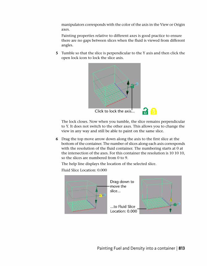
manipulators corresponds with the color of the axis in the View or Originaxes.
Painting properties relative to different axes is good practice to ensurethere are no gaps between slices when the fluid is viewed from differentangles.
5 Tumble so that the slice is perpendicular to the Y axis and then click theopen lock icon to lock the slice axis.
The lock closes. Now when you tumble, the slice remains perpendicularto Y. It does not switch to the other axes. This allows you to change theview in any way and still be able to paint on the same slice.
6 Drag the top move arrow down along the axis to the first slice at thebottom of the container. The number of slices along each axis correspondswith the resolution of the fluid container. The numbering starts at 0 atthe intersection of the axes. For this container the resolution is 10 10 10,so the slices are numbered from 0 to 9.
The help line displays the location of the selected slice.
Fluid Slice Location: 0.000
Painting Fuel and Density into a container | 813

7 In the Paint Attributes section of the Tool Settings window, ensure thatValue is set to 1. A Fuel value of 1 represents a totally unreacted statewhile a Fuel value of 0 represents a completely reacted state. A Densityvalue of 1 is totally opaque while a Density value of 0 is completelytransparent.
8 Drag the brush on the slice to paint values. Paint until the entire slice isfilled with values.
The values display as yellow because you are painting two properties atthe same time. Density values are represented by the opacity of the shadedvalues, while Fuel values are represented by color. The range of Fuel valuescorresponds with a ramp of colors from blue (values of 0) to yellow (valuesof 1).
To make the fluid deeper, you could move the slice to Fluid Slice Position1, paint, move the slice to Fluid Slice Position 2, paint, and so on. But aquicker way is to resize the slice to make it thicker and then flood theentire slice with values.
9 Resize the paint slice, making it thicker:
■ Click the target icon once to switch to the subvolume scaling mode.
814 | Chapter 16 Fluid Effects

The slice becomes thicker and the manipulator changes to include scalingboxes at the ends of the move arrows.
■ Click the top scaling box and read the help line to determine that theFluid Slice Thickness is 3.00. You could drag the scaling boxes tochange the thickness of the slice, but the slice is thick enough for thelesson.
10 In the Tool Settings window, click the Flood button.
Flooding filled each voxel in the subvolume with Fuel and Density valuesof 1.
Notice that the values display as shaded planes rather than as a solidmass. This is an interactive display feature for shaded display mode.Displaying more shaded planes (slices) produces more detail but reducesthe speed of the screen draw. You can change this display feature (SlicesPer Voxel) and others in the Display section of the Attribute Editor.
Now that the container has Density and Fuel in it, you are ready to starta reaction by adding Temperature. You could think of this as putting alit match into a container of gasoline.
Painting Fuel and Density into a container | 815

Painting Temperature values into a containerBy default, the Fuel and Density will react when there is no Temperature inthe container, but adding higher temperature values will make the reactionmore immediate.
To paint Temperature values into a container
1 In the Tool Settings window, beside Paintable Attributes, selectTemperature. A message appears prompting you to set the fluid’sTemperature method to Dynamic Grid or Static Grid.
By setting the Temperature method to Dynamic Grid, the temperaturevalues you place in the container grid are recalculated by the fluiddynamics solver and changed during simulation.
By setting the Temperature method to Static Grid, the temperature valuesyou place in the container grid are used by the fluid dynamics solverduring the simulation, but they cannot change during the simulation.Static Grid is useful when you want to define specific values in specificareas of the container, but you do not want these values to change overtime.
2 Click Set to Dynamic. The Density and Fuel values disappear. The valuesare still there, but only Temperature values now display. Currently thereare no temperature values in the container.
3 Change the brush so you can paint through the entire thickness of theslice with a single stroke. In the Stroke section of the Tool Settingswindow, change Stamp Depth (3D) to 2. The brush changes, showinghow deep the brush stroke will paint.
If you make the brush depth thicker than the depth of the slice, only thespace within the slice will be painted.
4 Paint a small amount of Temperature in the center of the slice.
816 | Chapter 16 Fluid Effects
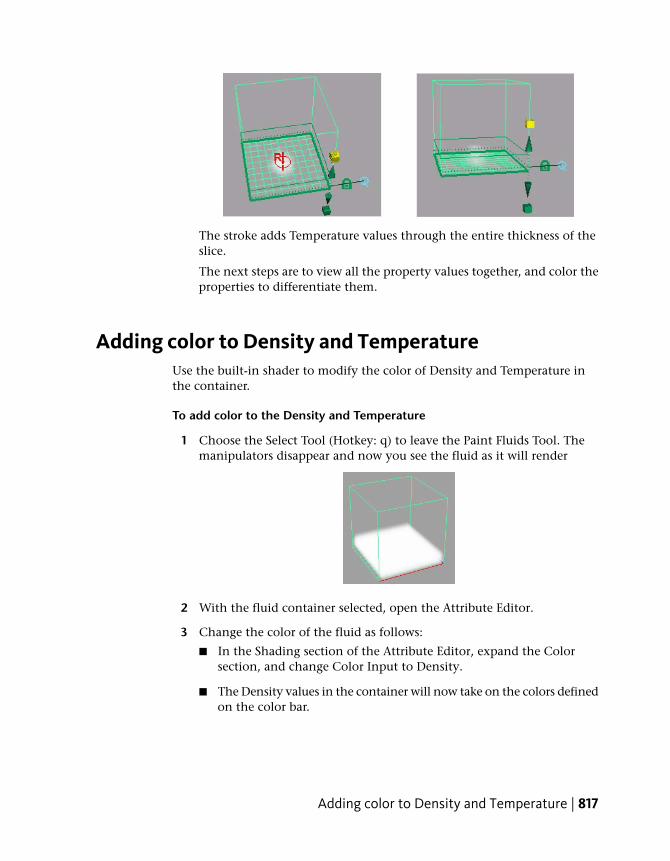
The stroke adds Temperature values through the entire thickness of theslice.
The next steps are to view all the property values together, and color theproperties to differentiate them.
Adding color to Density and TemperatureUse the built-in shader to modify the color of Density and Temperature inthe container.
To add color to the Density and Temperature
1 Choose the Select Tool (Hotkey: q) to leave the Paint Fluids Tool. Themanipulators disappear and now you see the fluid as it will render
2 With the fluid container selected, open the Attribute Editor.
3 Change the color of the fluid as follows:
■ In the Shading section of the Attribute Editor, expand the Colorsection, and change Color Input to Density.
■ The Density values in the container will now take on the colors definedon the color bar.
Adding color to Density and Temperature | 817

■ Click the Selected Color box. The Color Chooser opens.
■ Select black in the Color Chooser and click Accept.
The Density turns black.
Look closely at the center of the fluid. The area where you paintedTemperature has a reddish orange color. In the Incandescence section ofthe Attribute Editor, notice that Incandescence Input is set to Temperature.Temperature gives off light and Incandescence controls the amount oflight emitted from regions of Density due to self illumination. The rampdefines the color of this light.
4 Play the simulation using the playback controls at the bottom of theMaya window.
By frame 160, most of the Density values have reacted completely.
818 | Chapter 16 Fluid Effects

Beyond the lessonThis lesson introduced you to the Fuel and Temperature fluid properties. Youlearned how to:
■ Combine Fuel, Density, and Temperature to create a dynamic explosioneffect.
■ Add property values to a container by painting them.
■ Paint in a 3D container.
You can control how quickly the reaction takes place during the simulation,the temperature required to start the reaction, how much heat and light thereaction releases over time, and other aspects of the reaction using theattributes in the Fuel section under Contents Details in the fluidShape AttributeEditor.
For a more realistic look, you can also texture the fluid using the built-intexturing attributes in the Textures section.
For more information on Fuel and texturing attributes, see Fluid Effects in theMaya Help.
Lesson 4: Creating an ocean effect
Introduction
An ocean effect is defined by a plane with an ocean shader assigned to it.Ocean effects are not created with fluid containers like the dynamic andnon-dynamic fluid effects you created in the first three lessons.
Beyond the lesson | 819

A shader is a collection of attributes that define color and other surfacecharacteristics of the plane it is assigned to. For an ocean shader, theseattributes define realistic waves on large bodies of water.
In this lesson, you create an ocean, put a cube in it, and see how the cubefloats in the ocean. You learn how to:
■ Create an ocean plane and shader.
■ Create a preview plane to see the effects of the shader, includingdisplacement, without rendering.
■ Modify the ocean shader attributes to make the waves bigger.
■ Make an object a boat in the scene.
■ Modify the attributes for an expression that controls the buoyancy of theboat in the ocean.
Before beginning the lesson, do the steps in Preparing for the lessons on page790.
Creating an ocean plane and shaderFluid Effects simplifies the process of creating an ocean by providing a singlecommand that creates a plane that is optimized for best results, and an oceanshader with appropriate connections to the plane.
To create an ocean plane with ocean shader
1 Select Fluid Effects > Ocean > Create Ocean. Maya creates an ocean planeand assigns an ocean shader to it.
2 Dolly out to see the plane.
820 | Chapter 16 Fluid Effects
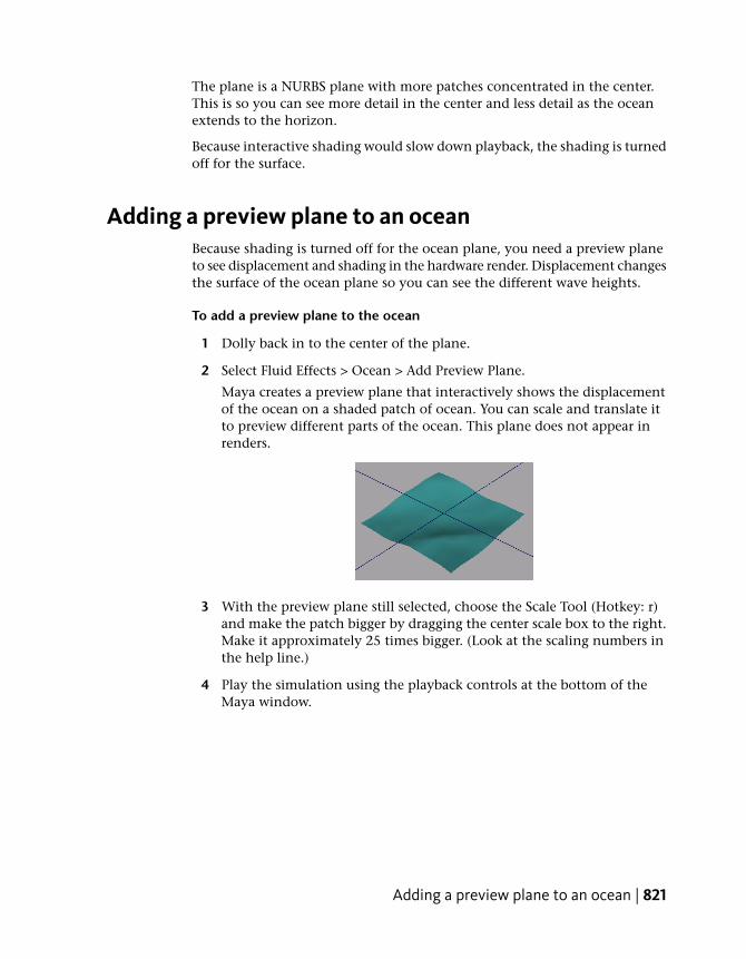
The plane is a NURBS plane with more patches concentrated in the center.This is so you can see more detail in the center and less detail as the oceanextends to the horizon.
Because interactive shading would slow down playback, the shading is turnedoff for the surface.
Adding a preview plane to an oceanBecause shading is turned off for the ocean plane, you need a preview planeto see displacement and shading in the hardware render. Displacement changesthe surface of the ocean plane so you can see the different wave heights.
To add a preview plane to the ocean
1 Dolly back in to the center of the plane.
2 Select Fluid Effects > Ocean > Add Preview Plane.
Maya creates a preview plane that interactively shows the displacementof the ocean on a shaded patch of ocean. You can scale and translate itto preview different parts of the ocean. This plane does not appear inrenders.
3 With the preview plane still selected, choose the Scale Tool (Hotkey: r)and make the patch bigger by dragging the center scale box to the right.Make it approximately 25 times bigger. (Look at the scaling numbers inthe help line.)
4 Play the simulation using the playback controls at the bottom of theMaya window.
Adding a preview plane to an ocean | 821

The preview plane ripples slightly showing the small wave displacement.
5 Light the scene to prepare it for rendering later in the lesson:
■ Select Create > Lights > Directional Light. Maya creates a directionallight called directionalLight1 at the center of the grid.
■ Open the Attribute Editor and in the Directional Light Attributessection of the directionalLightShape1 tab, change Intensity to 2 tomake the light brighter.
■ Click the directionalLight1 tab and rotate the light as follows to directthe light rays onto the ocean. Rotate: -100 42 20
Modifying ocean attributesIn the next steps, you will modify ocean shader settings to make the wavesbigger.
To modify attributes for the ocean shader
1 Render the current frame to see what the ocean looks like before youmodify the ocean shader attributes. On the Status line, click the rendercurrent frame icon.
822 | Chapter 16 Fluid Effects
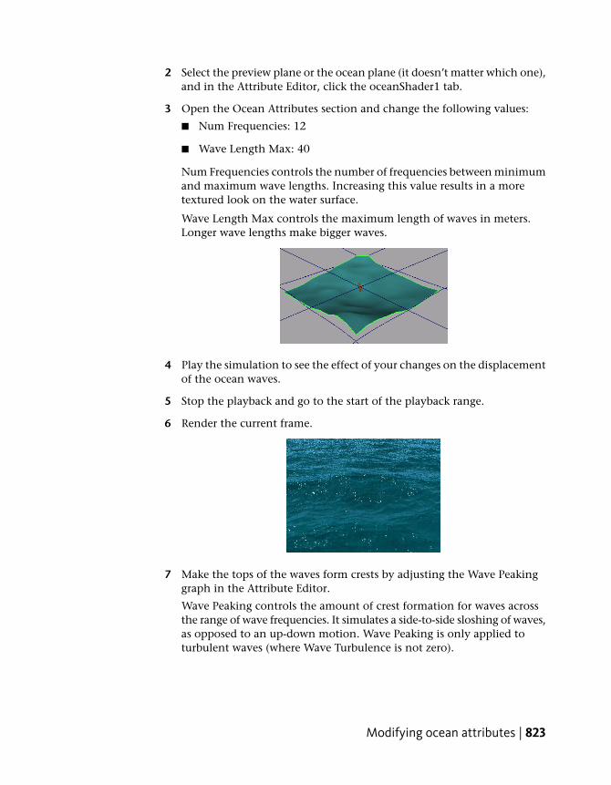
2 Select the preview plane or the ocean plane (it doesn’t matter which one),and in the Attribute Editor, click the oceanShader1 tab.
3 Open the Ocean Attributes section and change the following values:
■ Num Frequencies: 12
■ Wave Length Max: 40
Num Frequencies controls the number of frequencies between minimumand maximum wave lengths. Increasing this value results in a moretextured look on the water surface.
Wave Length Max controls the maximum length of waves in meters.Longer wave lengths make bigger waves.
4 Play the simulation to see the effect of your changes on the displacementof the ocean waves.
5 Stop the playback and go to the start of the playback range.
6 Render the current frame.
7 Make the tops of the waves form crests by adjusting the Wave Peakinggraph in the Attribute Editor.
Wave Peaking controls the amount of crest formation for waves acrossthe range of wave frequencies. It simulates a side-to-side sloshing of waves,as opposed to an up-down motion. Wave Peaking is only applied toturbulent waves (where Wave Turbulence is not zero).
Modifying ocean attributes | 823

Click on the graph to create the position markers shown in the nextillustration.
Where the wave frequency is lower, the waves peak more.
8 Render the current frame.
The tops of the waves now crest slightly.
Notice the white highlights on the ocean. These are specular highlightscaused by the light hitting the water.
9 Make the highlights dimmer so they don’t pop out as much, and bigger.Open the Specular Shading section and change the following settings:
■ Specularity: 0.45
■ Eccentricity: 0.1
Specularity controls the brightness of the specular highlights. Highervalues create brighter highlights.
Eccentricity controls the size of the specular highlights. Higher valuescreate bigger highlights.
824 | Chapter 16 Fluid Effects

10 Render the current frame.
Floating objectsYou can make geometry (for example, a boat) float in the ocean, movingappropriately with the motion of waves. The following steps show you howusing a simple polygon cube.
To float a cube in the ocean
1 Create a polygon cube (Select Create > Polygon Primitives > Cube).
2 In the Attribute Editor, click the pCube1 tab and scale the cube as follows:
■ Scale: 10 10 10
3 Select both the cube and the ocean plane (not the preview plane) at thesame time and select Fluid Effects > Ocean > Make Boats.
Maya creates a boat locator at the center of the cube to mark the cube’sposition in space. The locator is connected to a predefined expressionthat simulates buoyancy effects. The expression is connected to the waveheights (displacement) of the ocean.
To learn more about expressions, look at the Expressions lessons inGetting Started with Maya.
Floating objects | 825
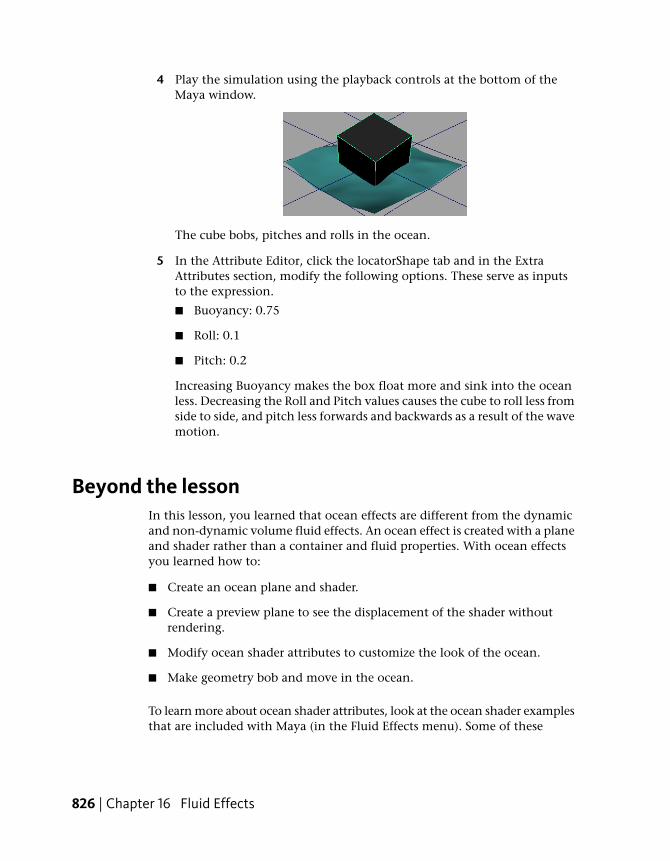
4 Play the simulation using the playback controls at the bottom of theMaya window.
The cube bobs, pitches and rolls in the ocean.
5 In the Attribute Editor, click the locatorShape tab and in the ExtraAttributes section, modify the following options. These serve as inputsto the expression.
■ Buoyancy: 0.75
■ Roll: 0.1
■ Pitch: 0.2
Increasing Buoyancy makes the box float more and sink into the oceanless. Decreasing the Roll and Pitch values causes the cube to roll less fromside to side, and pitch less forwards and backwards as a result of the wavemotion.
Beyond the lessonIn this lesson, you learned that ocean effects are different from the dynamicand non-dynamic volume fluid effects. An ocean effect is created with a planeand shader rather than a container and fluid properties. With ocean effectsyou learned how to:
■ Create an ocean plane and shader.
■ Create a preview plane to see the displacement of the shader withoutrendering.
■ Modify ocean shader attributes to customize the look of the ocean.
■ Make geometry bob and move in the ocean.
To learn more about ocean shader attributes, look at the ocean shader examplesthat are included with Maya (in the Fluid Effects menu). Some of these
826 | Chapter 16 Fluid Effects

examples use a 3D non-dynamic volume fluid to create the atmosphere abovethe ocean.
Motor Boats
You can create a game-style boat simulation using the Fluid Effects > Ocean> Make Motor Boats command. Once you set up hotkeys for the rudder andthrottle of the boat, you can “drive” the boat in the ocean. The boat will roll,pitch, and jump over waves appropriately.
Boat Wakes
You can create boat wakes using the Fluid Effects > Ocean > Create Wakecommand. Wake fluids do not use the Navier Stokes solver like regular fluids,but use the Spring Mesh Solver. A fluid emitter is used to drive the motion ofthe fluid.
Ponds
If a smaller body of water is what you had in mind, you can create a pondusing Fluid Effects > Pond > Create Pond. Ponds are 2D fluids that use a springmesh solver and a height field. You can generate bubbles, ripples, and wavesusing the Create Wake options for the pond.
For details on these topics and others, see Fluid Effects in the Maya Help.
Beyond the lesson | 827

828

Fur
Introduction
With the Maya® FurTM feature, you can create fur and short hair on all surfacetypes in Maya. A fur description in Maya defines all the attributes for the fur (forexample, fur color, width, length, baldness, opacity, curl, density, and so on).When applying fur, you can use one of the predefined fur descriptions includedwith Maya, or you can create your own custom fur description by setting allthe fur attributes yourself.
You can animate fur with keyframe effects like growing fur or changing color.For a more natural appearance, you can also add movement to fur with dynamics(for example, wind and gravity).
This chapter includes these lessons:
■ Lesson 1 Assigning a fur description: Introduction on page 830
17
829

■ Lesson 2 Rendering fur: Introduction on page 855
Preparing for the lessonsTo ensure the lessons work as described, do these steps before beginning:
1 If you have not already done so, copy the GettingStarted folder fromits installation location to your projects directory. Then, set theGettingStarted/Fur directory as your Maya project. For moreinformation, see Copying and setting the Maya project on page 25 in theGetting Started with Maya guide.
2 Select the Rendering menu set. Unless otherwise noted, the directions inthis chapter for making menu selections assume you’ve already selectedthe Rendering menu set
3 If you don’t see a Fur menu, perform these additional steps:
■ Select Window > Settings/Preferences > Plug-in Manager.
■ In the Plug-in Manager, locate the Fur plug-in (Fur.mll) and turn onthe loaded checkbox. Wait for the check mark to appear in thecheckbox, then close the Plug-in Manager. You can set the Fur plug-into auto load so that it automatically loads each time the Mayaapplication is launched. The Fur menu will appear to the right of thePaint Effects menu.
Lesson 1: Assigning a fur description
IntroductionMaya provides many predefined fur descriptions. These fur descriptions, alsoreferred to as presets, can be used as a starting point in creating fur for a model.Fur description presets can also be customized.
In this lesson you learn how to:
■ Duplicate parts of a model across its axis of symmetry.
■ Rename surfaces.
■ Assign surfaces to display layers.
830 | Chapter 17 Fur

■ Apply a fur description preset to the surfaces of a model.
■ Reverse surface normals on surfaces to ensure the fur description is orientedcorrectly.
■ Change the direction of the fur description on some of the surfaces.
■ Paint a fur attribute map to modify the fur length in an area of a surface.
■ Modify the fur color attributes of a fur description.
■ Create a new fur description for a surface and modify its attributes.
Lesson setupTo ensure the lesson works as described, do these steps before beginning:
➤ Open the scene named furStart.mb that is located in theGettingStarted/Fur/scenes directory of your Maya project.
This scene includes a model that has been created for you.
Duplicating objects across an axis of symmetry3D artists often construct one half of a symmetrical model in order to simplifythe data requirements. The scene provided for this lesson reflects this situation.
The teddy bear has only one half of its body. In the next steps, you’ll duplicatethe surfaces that make up the arms, legs, and body across the center axis tocomplete the model.
Lesson setup | 831
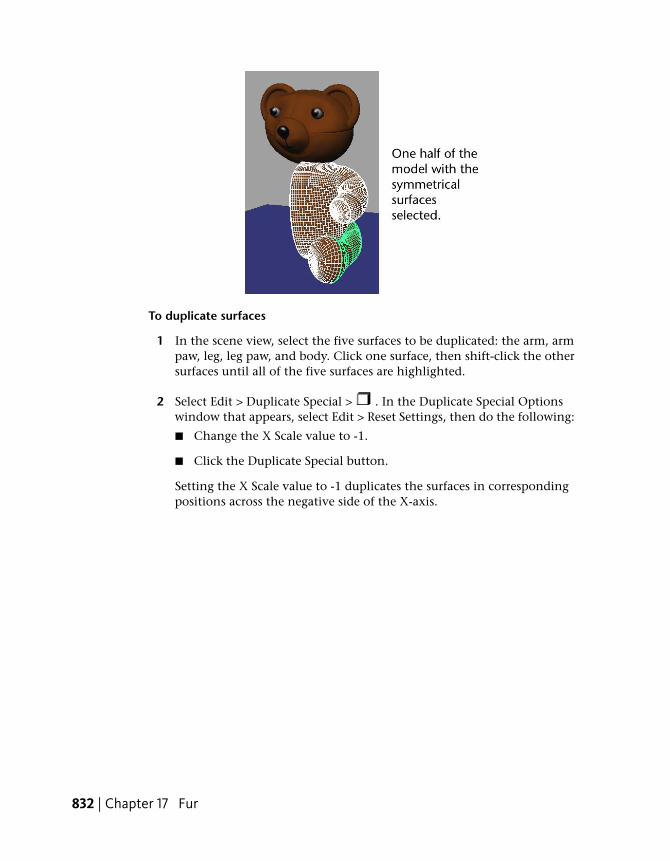
To duplicate surfaces
1 In the scene view, select the five surfaces to be duplicated: the arm, armpaw, leg, leg paw, and body. Click one surface, then shift-click the othersurfaces until all of the five surfaces are highlighted.
2 Select Edit > Duplicate Special > . In the Duplicate Special Optionswindow that appears, select Edit > Reset Settings, then do the following:
■ Change the X Scale value to -1.
■ Click the Duplicate Special button.
Setting the X Scale value to -1 duplicates the surfaces in correspondingpositions across the negative side of the X-axis.
832 | Chapter 17 Fur

Renaming surfaces on a modelAfter duplicating the surfaces you need to rename the duplicated surfaces soyou can easily identify and select them by name when required.
The surfaces you duplicated were originally named using the namingconvention leftArm, leftArmpaw, leftLeg, and leftLegpaw. When you duplicateobjects, Maya assigns names to the new objects automatically. Change thenames of the duplicated surfaces to match the naming convention used forthe model.
To rename objects
➤ For each of the surfaces listed in the following table, do the following:
■ Click the object in the scene view.
■ In the Channel Box, click the object name to select it. You can displaythe Channel Box by clicking Show/Hide Channel Box/Layer Editorbutton on the Status Line.
■ Type the corresponding new name from the table and press Enter.New nameOld name
rightArmleftArm1
rightArmpawleftArmpaw1
Renaming surfaces on a model | 833

New nameOld name
rightLegleftLeg1
rightLegpawleftLegpaw1
rightBodyleftBody1
Assigning objects to a reference layerIn this section you will assign any objects that will not have fur assigned toa referenced display layer so they become temporarily unselectable whenadding or changing a fur description.
Layers are overlapping views of your scene that can have objects assigned tothem. You can assign any objects within a scene to layers. One usefulcharacteristic of layers is that they let you simplify your scene so you can workon specific objects without disturbing other objects. You can choose whichobjects of the scene you want to assign to a layer and then selectively makethem visible or invisible. You can also template or reference all objectsassociated with a given layer.
To assign objects to a display layer
1 If the Channel Box isn’t already displayed, click the Show/Hide ChannelBox/Layer Editor button in the Status Line to display the Layer Editor
.
2 Ensure the Layer Editor is set to Display Layers by clicking the Displayradio button.
834 | Chapter 17 Fur
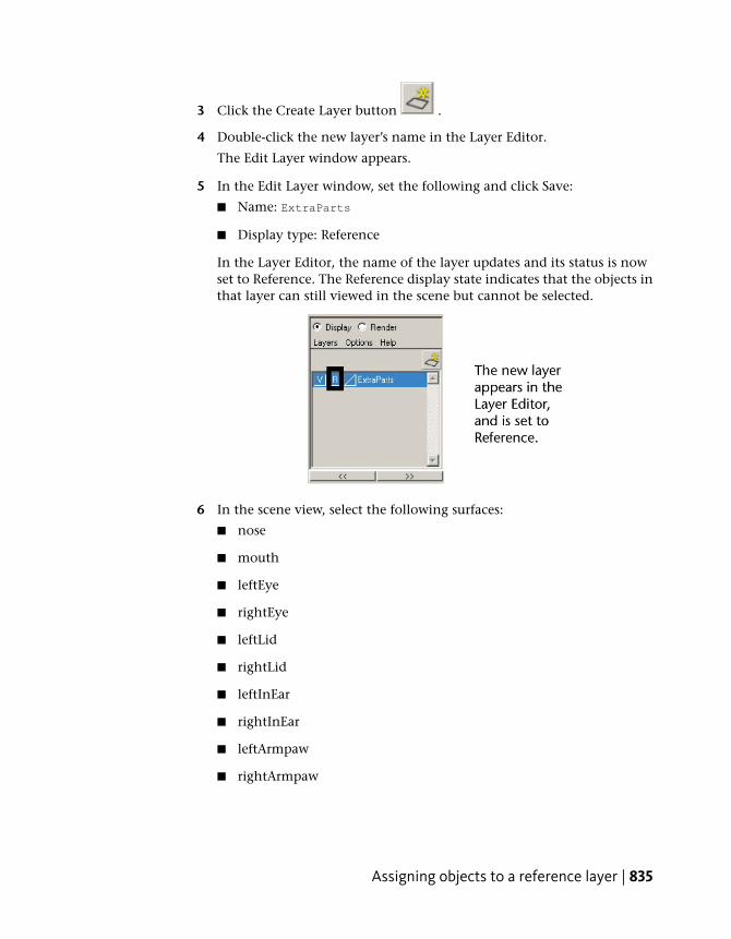
3 Click the Create Layer button .
4 Double-click the new layer’s name in the Layer Editor.
The Edit Layer window appears.
5 In the Edit Layer window, set the following and click Save:
■ Name: ExtraParts
■ Display type: Reference
In the Layer Editor, the name of the layer updates and its status is nowset to Reference. The Reference display state indicates that the objects inthat layer can still viewed in the scene but cannot be selected.
6 In the scene view, select the following surfaces:
■ nose
■ mouth
■ leftEye
■ rightEye
■ leftLid
■ rightLid
■ leftInEar
■ rightInEar
■ leftArmpaw
■ rightArmpaw
Assigning objects to a reference layer | 835

■ leftLegpaw
■ rightLegpaw
■ groundPlane
7 Right-click the ExtraParts layer in the Layer Editor and choose AddSelected Objects from the drop-down list that appears.
The selected objects are assigned to the ExtraParts display layer which iscurrently set to Reference. You can still view these objects but they cannotbe selected again until you set the display setting for this layer to Normal.Using reference layers in this fashion aids your workflow by ensuring youdon’t accidentally select unwanted surfaces when applying Fur.
Assigning a fur description preset to a modelA fur description defines all of the attributes for the fur, for example, fur color,width, length, baldness, opacity, curl, density, and so on. Maya includes a setof fur description presets you can use as is, or as a starting point in creatingyour own custom fur descriptions.
Any surfaces that should not have fur applied have already been assigned toa referenced display layer. This makes the application of a fur descriptioneasier.
836 | Chapter 17 Fur
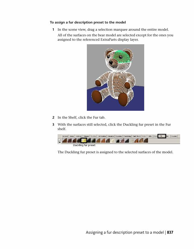
To assign a fur description preset to the model
1 In the scene view, drag a selection marquee around the entire model.
All of the surfaces on the bear model are selected except for the ones youassigned to the referenced ExtraParts display layer.
2 In the Shelf, click the Fur tab.
3 With the surfaces still selected, click the Duckling fur preset in the Furshelf.
The Duckling fur preset is assigned to the selected surfaces of the model.
Assigning a fur description preset to a model | 837

4 In the Channel Box, rename the Duckling fur description to TeddyBear.
Observe the yellow spikes that have appeared on the model. This is thefur feedback - a rough approximation of how the fur will appear whenrendered.
Fur feedback shows various fur attributes such as color, density, length,direction, and scraggle. By looking at the fur feedback you canimmediately see how the changes you make to the fur attributes affectthe appearance of the fur, without having to render the scene.
The fur feedback on the legs, arms, and top of the head of the modelappears different in comparison to how it appears on the body and snoutsurfaces. It should appear consistently on all of the assigned surfaces,which indicates that the surface normals may not be oriented consistentlyfor all of the assigned surfaces.
Reversing surface normalsWhen you apply a fur description to a surface, each hair making up the furdescription points in a direction normal (perpendicular) to the surface bydefault. This direction is called the surface normal. When the fur does notdisplay consistently on a model it may indicate that the surface normals areoriented inconsistently.
➤ Dolly the camera so you can view inside the arm.
838 | Chapter 17 Fur
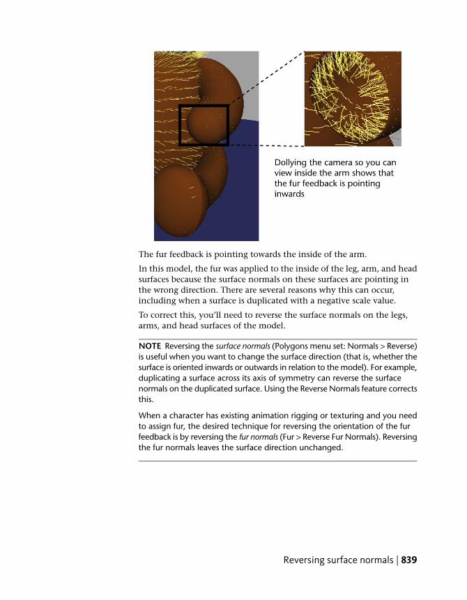
The fur feedback is pointing towards the inside of the arm.
In this model, the fur was applied to the inside of the leg, arm, and headsurfaces because the surface normals on these surfaces are pointing inthe wrong direction. There are several reasons why this can occur,including when a surface is duplicated with a negative scale value.
To correct this, you’ll need to reverse the surface normals on the legs,arms, and head surfaces of the model.
NOTE Reversing the surface normals (Polygons menu set: Normals > Reverse)is useful when you want to change the surface direction (that is, whether thesurface is oriented inwards or outwards in relation to the model). For example,duplicating a surface across its axis of symmetry can reverse the surfacenormals on the duplicated surface. Using the Reverse Normals feature correctsthis.
When a character has existing animation rigging or texturing and you needto assign fur, the desired technique for reversing the orientation of the furfeedback is by reversing the fur normals (Fur > Reverse Fur Normals). Reversingthe fur normals leaves the surface direction unchanged.
Reversing surface normals | 839

To reverse the surface normals
1 With only the legs, arms, and top head surfaces selected, switch to the
Polygons menu set and then select Normals > Reverse > .
2 Set the Reverse normals on setting to Selected faces and then click ReverseNormals.
The normals of the selected polygon surfaces are reversed so that the furdescription points in the correct direction.
Before proceeding to the next section, return to the Rendering menu set.
Modifying the fur directionReal fur usually doesn’t stick straight out of a surface but appears angled in aparticular direction. The teddy bear’s fur appears to point in different directionsdepending on the particular surface.
In this section, you modify the direction of the fur so it points in a consistentfashion on the model. You’ll also modify the direction of the fur to simulatea seam along the center of the bear’s forehead like a real stuffed toy mighthave.
840 | Chapter 17 Fur

There are three methods for modifying the direction of fur. Each method hasspecific conditions for use. You can modify the direction of fur by:
■ Modifying the Inclination, Polar, and Roll attributes for the fur descriptionglobally.
■ Setting a Fur Direction Offset to change the fur feedback direction locallyon a selected surface.
■ Combing the fur feedback locally on a surface using Maya’s Paint FurAttributes tool.
Modifying the Inclination, Polar, and Roll attributes for the assigned furdescription changes the direction attributes on the fur description globally.You can set these attributes using either the Channel Box or the AttributeEditor. Inclination sets the angle or slope at which the fur description willlean in relation to the surface. Polar sets the direction the fur description willpoint in relation to the surface normal, much like the hands on a clock face.Roll sets the angle about which the fur description will be rotated about itsfollicle and is used mostly when the fur has curl attributes applied. That is,you can control whether the curls point up, down, or lay flat on their side.
Modifying these attributes is a good starting point for creating a realistic furdescription. For the original Duckling fur description preset the Inclination,Polar, and Roll attributes are set to 0.6, 0.5, and 0.5 respectively. You won’tneed to change these for this lesson.
However, when a model is comprised of many surfaces, the fur may have atendency to point in a different direction on each separate surface dependingon how the surfaces were originally constructed.
To correct this you can change the direction of the fur using the Fur DirectionOffset. The Fur Direction Offset lets you change the orientation of a furdescription locally on a per-surface basis by applying a relative rotation valueto the fur description as it is applied to the selected surface.
To modify the fur direction using the Fur Direction Offset
1 Dolly the camera closer to the bear’s head so you can more closely viewthe direction of the fur description on the bear’s snout.
The fur appears to point in a clockwise direction about the bear’s snout.You can change the direction the fur points by changing the Fur DirectionOffset value for the bear’s snout.
2 Select the snout surface.
Modifying the fur direction | 841

3 Select Fur > Offset Fur Direction and click on the double lines at the topof the menu that appears so you can tear off the Offset Fur Directionmenu.
The Offset Fur Direction menu lets you rotate a fur description on aselected surface using direction presets.
4 Click on the 0, 90, 180, and 270 degree presets one at a time until thefur feedback on the snout points toward the bear’s face.
5 Repeat this process for the remaining surfaces that have fur assigned byselecting each surface one at a time and orienting the direction of the furfeedback as follows:
■ The fur feedback on the arms and legs should point in a directiontowards the paws.
■ The fur feedback on the body surfaces should point downwards.
■ The fur feedback on the head surfaces should point away from thecenter line so it simulates a sewn seam.
■ The fur feedback on the outer ear surfaces should point away fromthe bears head.
TIP Dolly and tumble the camera as you work to ensure you have the furfeedback oriented correctly. Try each offset direction so you know itseffect on the fur feedback on each surface. You can easily set the directionoffset back to its previous setting if it appears incorrect.
6 Close the Offset Fur Direction menu when you are finished orienting thefur feedback for all of the surfaces that have fur assigned.
842 | Chapter 17 Fur

Painting fur attributesThe fur feedback on the bear’s snout appears too long in the region of thebear’s mouth and nose. The fur will poke through the nose and hide the mouthin the final rendered image unless you shorten the fur in that region on thesnout. You can reduce the length of fur in a localized area of a surface usingthe Paint Fur Attributes Tool.
Using the Paint Fur Attributes Tool you can paint virtually any fur attribute.In this lesson you use the Paint Fur Attributes Tool to:
■ reduce the fur length in a localized area on a surface. This is useful whenyou want regions with shorter or longer fur on a surface.
■ create bald regions on a surface. This is useful for creating localized fureffects such as a moustache or goatee on a character, or whiskers on ananimal.
The Paint Fur Attributes Tool does all of the above via attribute maps that youcreate by painting directly on the surface. The attribute map modifies theassociated fur attributes you have selected for modification based on theregions of black, white, or gray that you paint in the map.
Before you begin painting an attribute map you’ll want to hide the nose andmouth surfaces. Earlier in the lesson you assigned the nose and mouth surfacesto the ExtraParts reference layer to prevent them from being accidentallyselected in the scene view. To hide these objects you can set the referenceddisplay layer to invisible.
Painting fur attributes | 843

To hide the referenced display layer
➤ In the Display Layer Editor, make the ExtraParts layer invisible by clickingthe V that indicates that the layer is visible.
To shorten the fur using the Paint Fur Attributes Tool
1 In the scene view, select the snout surface.
2 Select Fur > Paint Fur Attributes Tool > .
The cursor updates to display as a paint brush indicating that the PaintFur Attribute Tool is active. The Paint Fur Attributes Tool Settings windowand the Paint Tool Settings editor appears. These windows let you set andcontrol which attributes get painted for an attribute map.
3 In the Paint Fur Attributes Tools Settings window, ensure the followingoptions are set:
■ Fur Attribute: Length
■ Fur Description: TeddyBear
844 | Chapter 17 Fur

4 In the Paint Tool Settings editor, set the following:
■ Brush - Radius (U): 0.2
■ Brush - Radius (L): 0.2
■ Brush - Profile: Soft
■ Paint Attributes - Paint Operation: Replace
■ Paint Attributes - Value: 0.2
These settings set the brush to paint a relatively small, soft edged region,with each stroke of the tool as you replace the existing fur with shorterfur.
5 Position the brush cursor over the centre of the bear’s snout and beginstroking in a small circular motion about the center of the snout.
Wherever you paint, the fur feedback updates and becomes shorter inlength.
Painting fur attributes | 845

6 In the Display section of the Paint Tool Settings editor turn on the ColorFeedback option.
The snout surface updates to display the fur length attribute map you arecurrently painting. The black region at the end of the snout indicates thearea you have just painted. This region of the attribute map indicateswhere the fur will be shorter in length when it is rendered. The lightergray region indicates where you have not yet painted and where the furlength will remain unaffected.
You also want the fur to be short in the region of the bear’s mouth aswell.
7 Paint a few overlapping strokes on the region of the snout below the nosewhere the mouth surface is located, as shown below.
846 | Chapter 17 Fur

Notice that the attribute map has a gradual color falloff. This ensures thatthe fur transition between the original attribute values and the map doesnot appear abrupt. You can smooth the attribute map even further byapplying a smooth operation.
8 In the Paint Tool Settings editor, set the Paint Operation to Smooth, andthen click Flood to apply a smooth to the entire fur length attribute map.You can click Flood more than once to apply multiple smooth operations.
TIP If you accidentally paint an area that is too large you can click Ctrl + zrepeatedly to undo your paint strokes.
If you want to begin painting the attribute map again, you can set the Valueto 1 and then click Flood to fill the surface with a white color.
To create whiskers using the Paint Fur Attributes Tool
1 Ensure that the snout surface is still active and click the Porcupine furpreset from the Fur shelf.
A second fur description is assigned to the bear’s snout. The snout appearscluttered at this point but you’ll rectify it in the following steps.
2 Ensure that the snout surface is still active and select Fur > Paint Fur
Attributes Tool > .
3 In the Paint Fur Attributes Tools Settings window, set the followingoptions:
■ Fur Attribute: Baldness
■ Fur Description: Porcupine
4 In the Paint Tool Settings editor, set the Paint Attributes - Paint Operationto Replace, Value to zero, and then click Flood.
This creates a baldness attribute map for the Porcupine fur descriptionthat is black in color making the Porcupine fur feedback disappeartemporarily.
Painting fur attributes | 847
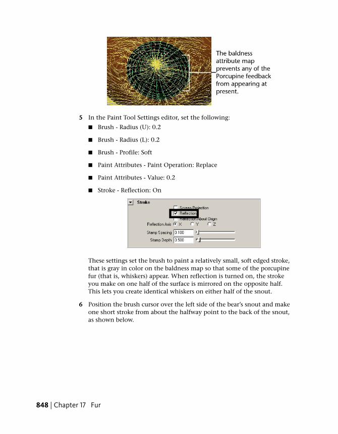
5 In the Paint Tool Settings editor, set the following:
■ Brush - Radius (U): 0.2
■ Brush - Radius (L): 0.2
■ Brush - Profile: Soft
■ Paint Attributes - Paint Operation: Replace
■ Paint Attributes - Value: 0.2
■ Stroke - Reflection: On
These settings set the brush to paint a relatively small, soft edged stroke,that is gray in color on the baldness map so that some of the porcupinefur (that is, whiskers) appear. When reflection is turned on, the strokeyou make on one half of the surface is mirrored on the opposite half.This lets you create identical whiskers on either half of the snout.
6 Position the brush cursor over the left side of the bear’s snout and makeone short stroke from about the halfway point to the back of the snout,as shown below.
848 | Chapter 17 Fur
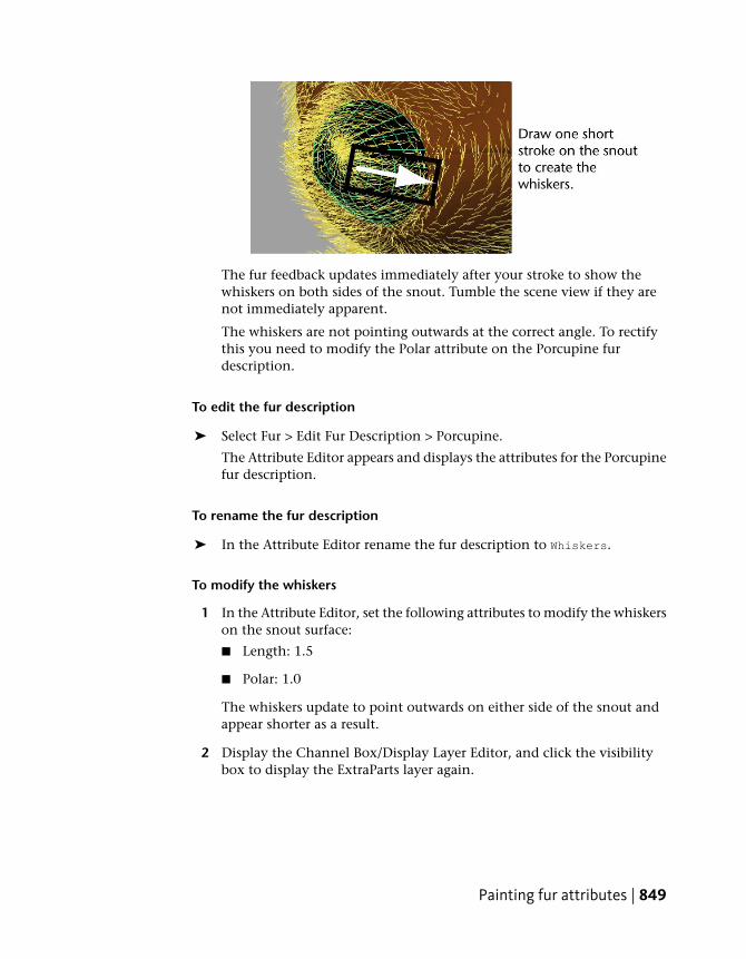
The fur feedback updates immediately after your stroke to show thewhiskers on both sides of the snout. Tumble the scene view if they arenot immediately apparent.
The whiskers are not pointing outwards at the correct angle. To rectifythis you need to modify the Polar attribute on the Porcupine furdescription.
To edit the fur description
➤ Select Fur > Edit Fur Description > Porcupine.
The Attribute Editor appears and displays the attributes for the Porcupinefur description.
To rename the fur description
➤ In the Attribute Editor rename the fur description to Whiskers.
To modify the whiskers
1 In the Attribute Editor, set the following attributes to modify the whiskerson the snout surface:
■ Length: 1.5
■ Polar: 1.0
The whiskers update to point outwards on either side of the snout andappear shorter as a result.
2 Display the Channel Box/Display Layer Editor, and click the visibilitybox to display the ExtraParts layer again.
Painting fur attributes | 849

Modifying the color of a fur descriptionNext you’ll change the color of the fur description so it resembles a real teddybear. To do this you’ll edit the fur description and set the Base and Tip Colorattributes using the Attribute Editor.
To modify the fur description
1 Select Fur > Edit Fur Description > TeddyBear.
The Attribute Editor appears and displays the attributes for the assignedTeddyBear fur description.
2 In the Attribute Editor, modify the Base and Tip Color attributes for theTeddyBear fur description by clicking the color swatches for each attribute,setting the RGB range to 0 to 255, and entering the following RGB values:
■ Base Color R: 62
■ Base Color G: 30
■ Base Color B: 8
■ Tip Color R: 106
■ Tip Color G: 52
■ Tip Color B: 14
These values change the color of the base of the fur to a dark brown, andthe tips of the fur a lighter brown. The fur feedback is updated on thebear model.
850 | Chapter 17 Fur

Creating a new fur descriptionTo make the bear appear more interesting you’ll assign a new fur descriptionto the inside of the ears and then modify fur attributes such as density, scraggle,and inclination.
Before you can assign a fur description to the inner ear surfaces you’ll needto select them by first turning off the referenced display layer.
To turn off the referenced display layer
1 Display the Channel Box/Display Layer Editor.
2 In the Display Layer Editor, click the box that displays the letter R untilthe box is empty.
To change the display state of a display layer, click repeatedly in themiddle box next to the layer name to cycle the display state fromReference (R), Template (T), or Normal (empty). When the box is emptythe display layer is no longer referenced and its possible to select all ofthe surfaces on the model.
To create a new fur description
1 In the scene view, select the following surfaces of the model:
■ leftInnerEar
Creating a new fur description | 851

■ rightInnerEar
2 Select Fur > Attach Fur Description > New.
A new default fur description is assigned to the selected surfaces.
To rename the fur description
1 Select Fur > Edit Fur Description > Fur Description1.
The Attribute Editor appears and displays the attributes for the new furdescription.
2 In the Attribute Editor rename the fur description to InnerEar.
To modify the color of the fur description
1 In the Attribute Editor, modify the Base and Tip Color attributes for theInnerEar fur description by clicking the color swatches for each attribute,setting the RGB range to 0 to 255, and entering the following RGB values:
■ Base Color R: 106
■ Base Color G: 52
■ Base Color B: 14
■ Tip Color R: 164
■ Tip Color G: 119
■ Tip Color B: 91
852 | Chapter 17 Fur
2 Modify these additional InnerEar attributes by entering the followingvalues:
■ Density: 50,000
■ Length: 0.25
■ Inclination: 0.8
■ Base Width: 0.2
■ Tip Width: 0
■ Scraggle: 0.1
Density specifies the number of hairs on a surface. The higher the value,the thicker the fur. Notice that changing the Density value does not affectthe fur feedback in the scene view; changes to fur density only appear inthe rendered image.
Length sets the fur’s length, in grid units.
Inclination sets how the fur slopes or leans. A value of 0 is fully erect(normal to the surface), while a value of 1 is flat (tangent to the surfaceat the root).
Base and Tip Width specifies width of the hairs at their base and tip.
Scraggle sets the crookedness of the fur. A value of 0 creates nocrookedness, while a value of 1 creates maximum crookedness.
The fur description for the Inner Ear surfaces is updated.
NOTE Some attributes of a fur description are only visible when you renderan image of the fur. You’ll render an image of the teddy bear fur in the nextlesson.
Beyond the lessonThe Teddy Bear now has brown fur and whiskers. The fur in the bear’s ears isa lighter brown color.
In this lesson you learned how to:
■ Duplicate surfaces across the axis of symmetry—you duplicated the armand body surfaces and created a mirror-copy of them.
Beyond the lesson | 853

■ Rename surfaces—Naming objects as you create them ensures you caneasily identify and select them later on.
■ Assign parts of a model to display layers—any surfaces that you did notwant fur applied were assigned to a referenced display layer so they wouldnot get selected accidentally.
■ Assign an existing fur description preset to a model—Fur presets are a usefulstarting point for creating various fur types. All of the fur presets includedwith Maya can be customized. You also created a new fur description forthe inner ear surfaces and customized its attributes.You can assign more than one fur description to a surface. In this lesson,you added a second fur description to the bear’s snout in order to createwhiskers.
■ Reverse surface normals so the fur was oriented to point in the correctdirection—Two methods are possible for correcting the normals; reversingthe surface normals, and reversing the fur normals.
■ Modify the direction of the fur description on individual surfaces usingthe Fur Description Offset—when a model is comprised of multiple surfacesthe fur description may point in different directions. You can modify thefur direction using a variety of techniques depending on the situation.
■ You modified the length of the fur description on the bear’s snout andcreated whiskers using the Paint Fur Attributes Tool. This tool lets youpaint an attribute map to modify specific fur attributes on an area of asurface.You can use the Paint Fur Attributes tool to paint the direction of the fur.This technique is also referred to as combing the fur because it resemblesthe stroking action you perform when combing real hair. Combing thefur feedback is useful when you need to hide a visible seam between twosurfaces.
■ Modify fur attributes—You learned how to modify the attributes of a furdescription using the Attribute Editor.Though not covered in this lesson, you can keyframe changes you maketo fur attributes to animate effects such as growing fur or changing furcolor. You can add movement to fur with attractors and dynamics. Usingattractors, you manually keyframe fur movement. Using dynamics, youcan make the fur react to forces, for example, wind and gravity. You canalso use dynamics to cause fur to react to movement of the attached surface,for example, when a dog shakes itself.
■ UV texture coordinates—When applying fur to a surface the UVs must belaid out so they are non-overlapping and reside between 0 and 1 in the
854 | Chapter 17 Fur
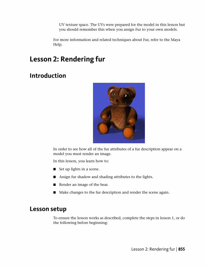
UV texture space. The UVs were prepared for the model in this lesson butyou should remember this when you assign Fur to your own models.
For more information and related techniques about Fur, refer to the MayaHelp.
Lesson 2: Rendering fur
Introduction
In order to see how all of the fur attributes of a fur description appear on amodel you must render an image.
In this lesson, you learn how to:
■ Set up lights in a scene.
■ Assign fur shadow and shading attributes to the lights.
■ Render an image of the bear.
■ Make changes to the fur description and render the scene again.
Lesson setupTo ensure the lesson works as described, complete the steps in lesson 1, or dothe following before beginning:
Lesson 2: Rendering fur | 855
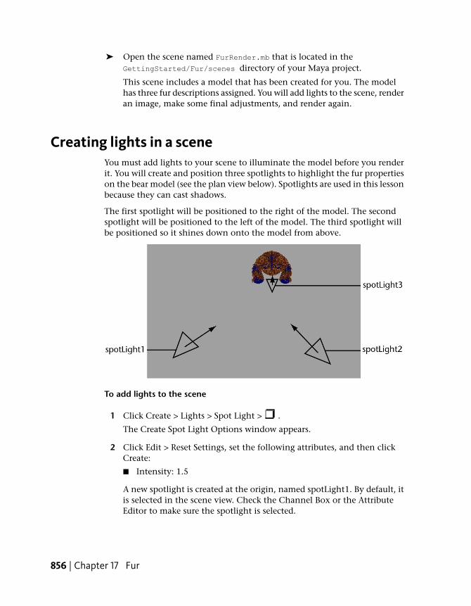
➤ Open the scene named FurRender.mb that is located in theGettingStarted/Fur/scenes directory of your Maya project.
This scene includes a model that has been created for you. The modelhas three fur descriptions assigned. You will add lights to the scene, renderan image, make some final adjustments, and render again.
Creating lights in a sceneYou must add lights to your scene to illuminate the model before you renderit. You will create and position three spotlights to highlight the fur propertieson the bear model (see the plan view below). Spotlights are used in this lessonbecause they can cast shadows.
The first spotlight will be positioned to the right of the model. The secondspotlight will be positioned to the left of the model. The third spotlight willbe positioned so it shines down onto the model from above.
To add lights to the scene
1 Click Create > Lights > Spot Light > .
The Create Spot Light Options window appears.
2 Click Edit > Reset Settings, set the following attributes, and then clickCreate:
■ Intensity: 1.5
A new spotlight is created at the origin, named spotLight1. By default, itis selected in the scene view. Check the Channel Box or the AttributeEditor to make sure the spotlight is selected.
856 | Chapter 17 Fur

3 In the Channel Box, enter the following values to reposition the spotlight:
■ Translate X: -39
■ Translate Y: 12
■ Translate Z: 34
■ Rotate X: -5
■ Rotate Y: -49
4 Click Create > Lights > Spot Light to create another spotlight at the origin.
This new spotlight will be named spotLight2 and have the same intensitysetting as the first spotlight.
5 In the Channel Box, enter the following values to reposition the secondspotlight:
■ Translate X: 25
■ Translate Y: 15
■ Translate Z: 35
■ Rotate X: -10
■ Rotate Y: 35
6 Click Create > Lights > Spot Light > , set the following attribute, andthen click Create:
■ Intensity: 0.5
A third spotlight is created at the origin, called spotLight3.
7 In the Channel Box, enter the following values to reposition the thirdspotlight:
■ Translate Y: 85
■ Translate Z: 7
■ Rotate X: -88
These three light sources will evenly illuminate the model: one will create ashadow once you have set fur shadowing attributes for the spotlights.
Creating lights in a scene | 857
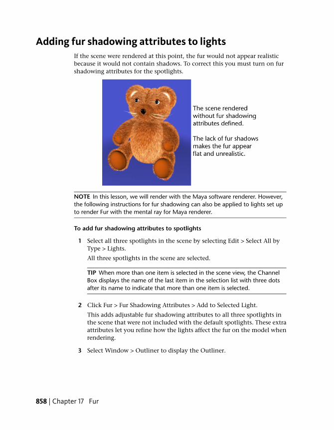
Adding fur shadowing attributes to lightsIf the scene were rendered at this point, the fur would not appear realisticbecause it would not contain shadows. To correct this you must turn on furshadowing attributes for the spotlights.
NOTE In this lesson, we will render with the Maya software renderer. However,the following instructions for fur shadowing can also be applied to lights set upto render Fur with the mental ray for Maya renderer.
To add fur shadowing attributes to spotlights
1 Select all three spotlights in the scene by selecting Edit > Select All byType > Lights.
All three spotlights in the scene are selected.
TIP When more than one item is selected in the scene view, the ChannelBox displays the name of the last item in the selection list with three dotsafter its name to indicate that more than one item is selected.
2 Click Fur > Fur Shadowing Attributes > Add to Selected Light.
This adds adjustable fur shadowing attributes to all three spotlights inthe scene that were not included with the default spotlights. These extraattributes let you refine how the lights affect the fur on the model whenrendering.
3 Select Window > Outliner to display the Outliner.
858 | Chapter 17 Fur

As your scene gets increasingly complex the Outliner becomes useful forselecting specific objects in the scene, especially when you want to selectobjects that are hidden by other objects, or are outside the camera’s fieldof view. Selecting items in the Outliner is much easier when you havenamed the objects and lights in your scene.
4 In the Outliner, click spotLight1 to select it in the scene.
5 Open the Attribute Editor by clicking the Show/Hide Attribute Editoricon on the Status Line.
6 Select the spotLightShape tab, and under Fur Shadowing/Shadowing, setthe Fur Shading Type to Shadow Maps.
7 In the Attribute Editor, under Shadows > Depth Map Shadow Attributes,set the following options:
■ Use Depth Map Shadows: On
■ Use Auto Focus: Off
■ Focus: 40
Depth Map Shadows are one technique for producing shadows in a sceneby determining which objects in the scene are in the path of a shadowcasting light.
Fur Shadows can be incorrectly placed when Auto Focus is turned on. Toavoid this, turn off Auto Focus for all spotlights that have Fur ShadowMaps turned on and instead set the Focus value to Cone Angle +(Penumbra * 2).
Adding fur shadowing attributes to lights | 859

8 Shift-select spotlight2 and spotlight3 using the Outliner.
9 In the Attribute Editor, under Fur Shadowing/Shadowing, set the FurShading Type to Auto Shading.
The Autoshade attribute provides a quick simulation of shading thatoccurs at the root and back of the fur strands without the addedcomplexity of a shadow map.
Rendering the sceneTo see the fur in full detail, you need to render an image of the scene.
To render the scene
1 Select Window > Rendering Editors > Render Settings to show the RenderSettings window.
2 Ensure that Render Using is set to Maya Software in the drop-down list.
3 From the Render Settings window menu, select Presets > Load Preset >Default Settings.
This sets the renderer to render an image that is 640 by 480 pixels in size;large enough to see the fine detail on the fur.
4 Close the Render Settings window.
5 To render the fur, do one of the following:
■ Select Render > Render Current Frame.
■ Click the Render Current Frame button in the Status Line.
The Render View window appears and an image of the scene is rendered.
860 | Chapter 17 Fur
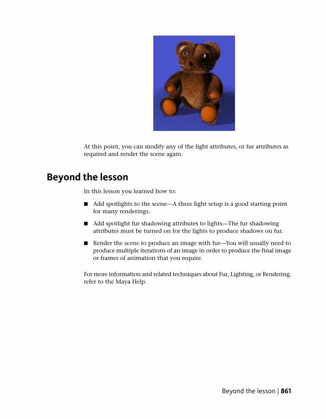
At this point, you can modify any of the light attributes, or fur attributes asrequired and render the scene again.
Beyond the lessonIn this lesson you learned how to:
■ Add spotlights to the scene—A three light setup is a good starting pointfor many renderings.
■ Add spotlight fur shadowing attributes to lights—The fur shadowingattributes must be turned on for the lights to produce shadows on fur.
■ Render the scene to produce an image with fur—You will usually need toproduce multiple iterations of an image in order to produce the final imageor frames of animation that you require.
For more information and related techniques about Fur, Lighting, or Rendering,refer to the Maya Help.
Beyond the lesson | 861

862

nCloth
Introduction
With the Maya® nCloth™ feature, you can create dynamic cloth effects in Maya.nCloth is a fast and stable dynamic cloth solution that uses a system of linkedparticles to simulate a wide variety of dynamic polygon surfaces, such as fabricclothing, inflating balloons, shattering surfaces, and deformable objects. nClothis generated from modeled polygon meshes. You can model any type of polygonmesh and make it an nCloth object, which is ideal for achieving specific posesand maintaining directorial control.
nCloth is built on a dynamic simulation framework called Maya® Nucleus™. AMaya Nucleus system is composed of a series of nCloth objects, passive collisionobjects, dynamic constraints, and a Maya Nucleus solver. As part of the MayaNucleus system, the Maya Nucleus solver calculates nCloth simulation, collisions,and constraints in an iterative manner, improving the simulation after eachiteration, to produce accurate cloth behavior.
18
863

Maya provides many predefined nCloths. These sample nCloth objects, alsoreferred to as presets, can be used as a starting point in creating your owncustom cloth effects.
This chapter includes these lessons:
■ Lesson 1: Creating nCloth collisions on page 865
■ Lesson 2: Creating nCloth constraints on page 880
■ Lesson 3: Creating nCloth Clothing on page 895
Preparing for the lessonsTo ensure the lessons work as described, do these steps before beginning:
1 Make sure you understand the basic concepts of polygon modeling,animation, and dynamics.
2 If you have not already done so, copy the GettingStarted folder fromits installation location to your projects directory. Then, set theGettingStarted directory as your Maya project. For more information,see Copying and setting the Maya project on page 25 in the GettingStarted with Maya guide.
3 Select the nDynamics menu set. Unless otherwise noted, the directionsin this chapter for making menu selections assume you’ve already selectedthe nDynamics menu set.
864 | Chapter 18 nCloth
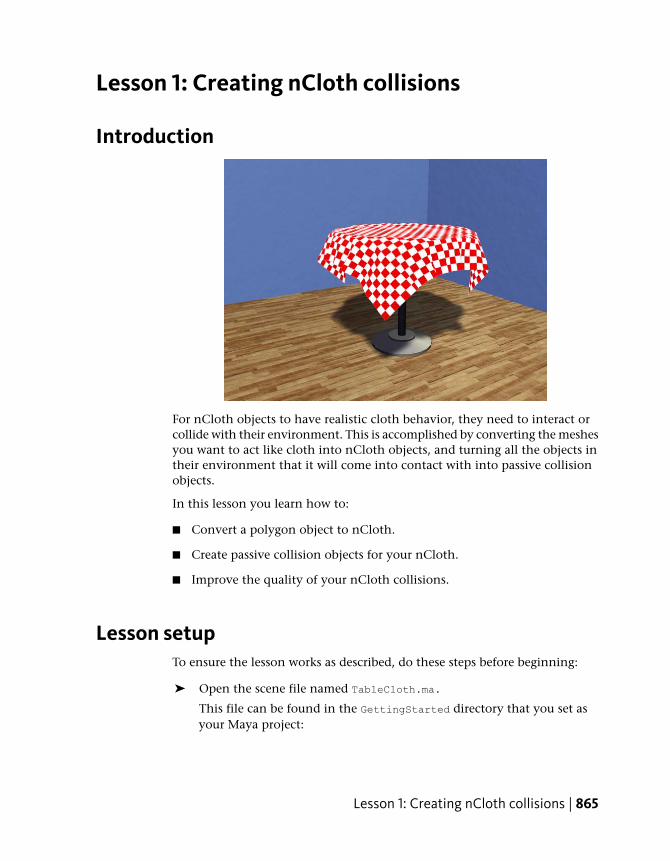
Lesson 1: Creating nCloth collisions
Introduction
For nCloth objects to have realistic cloth behavior, they need to interact orcollide with their environment. This is accomplished by converting the meshesyou want to act like cloth into nCloth objects, and turning all the objects intheir environment that it will come into contact with into passive collisionobjects.
In this lesson you learn how to:
■ Convert a polygon object to nCloth.
■ Create passive collision objects for your nCloth.
■ Improve the quality of your nCloth collisions.
Lesson setupTo ensure the lesson works as described, do these steps before beginning:
➤ Open the scene file named TableCloth.ma.
This file can be found in the GettingStarted directory that you set asyour Maya project:
Lesson 1: Creating nCloth collisions | 865

GettingStarted/nCloth/TableCloth.ma
This scene includes textured models that have been created for you. Thetable cloth, table, table base, floor, and wall models provided are allpolygon meshes.
Creating an nCloth object
The first step in the nCloth creation process is to convert the polygon objectyou want to behave like cloth to an nCloth object.
To make a polygon mesh nCloth
1 Select the checkered table cloth.
2 Select nMesh > Create nCloth > .
The Create Cloth Options window appears.
3 Select nucleus1 from the Solver drop-down list.
866 | Chapter 18 nCloth
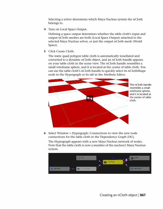
Selecting a solver determines which Maya Nucleus system the nClothbelongs to.
4 Turn on Local Space Output.
Defining a space output determines whether the table cloth’s input andoutput nCloth meshes are both (Local Space Output) attached to theselected Maya Nucleus solver, or just the output nCloth mesh (WorldSpace).
5 Click Create Cloth.
The static quad polygon table cloth is automatically tessellated andconverted to a dynamic nCloth object, and an nCloth handle appearson your table cloth in the scene view. The nCloth handle resembles asmall wireframe sphere, and it is located at the center of table cloth. Youcan use the table cloth’s nCloth handle to quickly select its nClothShapenode in the Hypergraph or its tab in the Attribute Editor.
6 Select Window > Hypergraph: Connections to view the new nodeconnections for the table cloth in the Dependency Graph (DG).
The Hypergraph appears with a new Maya Nucleus network of nodes.Note that the table cloth is now a member of the nucleus1 Maya Nucleussystem.
Creating an nCloth object | 867

nClothShape1 is the nCloth properties node, which carries all the nClothattributes for the table cloth.
nucleus1 is the Maya Nucleus solver node, which carries all the attributesaffecting the nucleus1 solver system, including internal forces.
TableClothShape is the input mesh and start object for the table cloth.
outputCloth1 is the output mesh or current mesh, and the resulting nClothtable cloth that you see in the scene view.
polyPlane2 is the history node for the table cloth.
7 Close the Hypergraph and play back your table cloth’s simulation.
The table cloth passes right through the table, its base, and the floor. Thisis because the nCloth does not recognize any of the other objects in yourscene. For the nCloth table cloth to be able to interact with the table, itsbase, and the floor, they need to be members of the same Maya Nucleussolver system as the table cloth.
8 Go to the beginning of the playback range.
Making an nCloth collide with its environmentThe second step in creating realistic cloth effects is to make your nCloth objectinteract with its environment, and have the objects and surfaces in its scenedeform the nCloth and drive its movements. You can do this by making eachsurface the nCloth comes into contact with during its simulation passive collisionobjects.
868 | Chapter 18 nCloth
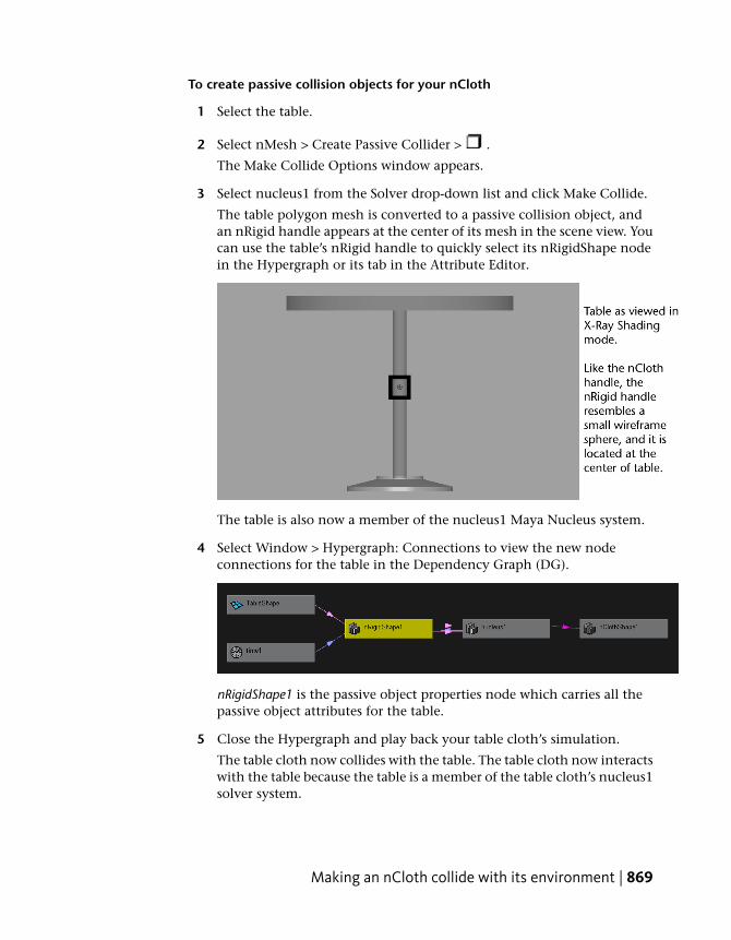
To create passive collision objects for your nCloth
1 Select the table.
2 Select nMesh > Create Passive Collider > .
The Make Collide Options window appears.
3 Select nucleus1 from the Solver drop-down list and click Make Collide.
The table polygon mesh is converted to a passive collision object, andan nRigid handle appears at the center of its mesh in the scene view. Youcan use the table’s nRigid handle to quickly select its nRigidShape nodein the Hypergraph or its tab in the Attribute Editor.
The table is also now a member of the nucleus1 Maya Nucleus system.
4 Select Window > Hypergraph: Connections to view the new nodeconnections for the table in the Dependency Graph (DG).
nRigidShape1 is the passive object properties node which carries all thepassive object attributes for the table.
5 Close the Hypergraph and play back your table cloth’s simulation.
The table cloth now collides with the table. The table cloth now interactswith the table because the table is a member of the table cloth’s nucleus1solver system.
Making an nCloth collide with its environment | 869

NOTE You may need to increase the total number of frames on your timeline for the table cloth to collide with the table.
Adjusting the accuracy of nCloth collisionsThe third step in creating believable cloth effects is to make your nClothobject’s collisions as accurate as possible. In reality, a falling piece of clothcomes into close contact with the object it lands on and it deforms, reflectingthe shape of the object it has come into contact with. Currently, the tablecloth does not exhibit this behavior.
To set the thickness of your nCloth and passive objects
1 Select the table cloth.
2 Open the Attribute Editor and select the nClothShape1 tab.
3 In the Collisions section, select Collision Thickness from the SolverDisplay drop-down list.
870 | Chapter 18 nCloth

The table cloth’s collision thickness appears in the scene view.
An nCloth’s Thickness attribute determines the radius or depth of thetable cloth’s collision volume. The collision volume is a non-renderablesurface offset from the table cloth’s surface that the nucleus1 solver useswhen calculating the table cloth’s passive object collisions. Collisionsoccur at the table cloth’s collision volume, not at the surface of the tablecloth itself.
Adjusting the accuracy of nCloth collisions | 871

4 Go to the beginning of the playback range.
5 In the Collisions section, change the table cloth’s Thickness attributevalue to 0.066.
The table cloth’s collision volume is noticeably reduced, so that it willnow behave like a thin piece of fabric rather than a thick surface. Thisnew Thickness will contribute to improving the accuracy of the tablecloth’s collisions when it falls onto the table.
6 Select Off from the Solver Display drop-down list.
872 | Chapter 18 nCloth

The table cloth’s Collision Thickness is no longer displayed in the sceneview.
7 Play back the table cloth’s simulation.
Even though you adjusted the table cloth’s Thickness, the table cloth stilldoes not appear to be making contact with the table’s surface. This isbecause passive collision objects, like the table, also possess collisionvolumes.
Adjusting the accuracy of nCloth collisions | 873

To further improve the accuracy of the table cloth’s collisions, you needto adjust the table’s Thickness.
8 Go to the beginning of the playback range.
9 In the scene view select the table, and in the Attribute Editor select itsnRigidShape1 tab.
10 In the Collisions section, select Collision Thickness from the SolverDisplay drop-down list.
The table’s collision thickness appears in the scene view.
11 Set the table’s Thickness attribute value to 0.066.
874 | Chapter 18 nCloth

The table’s collision volume is noticeably reduced, so that the table clothwill now conform closely to the actual shape of the table when you playback its simulation.
12 In the Collisions section, select Off from the Solver Display drop-downlist.
The table’s Collision Thickness is no longer displayed in the scene view.
13 Play back the table cloth’s simulation.
Adjusting the accuracy of nCloth collisions | 875

Adjusting the Thickness of the table cloth nCloth and the table passiveobject dramatically improved the accuracy of the table cloth’s collisions.
14 Go to the start of the playback range.
The way Collision Thickness appears in the scene view is determined by yournCloth’s current Collision Flag selection. The Collision Flag drop-down list letsyou specify which of the table cloth’s components participate in its collisionsand which type of collision volume is used by the table cloth. You can adjustthe speed of your nCloth collisions with the Collision Flag at the cost ofcollision accuracy.
876 | Chapter 18 nCloth

To set which nCloth components participate in collisions
1 Select the table cloth.
2 In the Attribute Editor, select the nClothShape1 tab.
3 In the Collisions section, select Collision Thickness from the SolverDisplay drop-down list.
4 By default, the Collision Flag is set to Face.
Face provides the best and most accurate collisions, but it is the slowestto calculate the collisions for.
5 Change the Collision Flag selection to Vertex. Vertex produces the leastaccurate collisions, but it is the fastest to calculate the collisions for.
The table cloth’s collision volume changes from a surface to multiplecollision spheres.
6 Play back the table cloth’s simulation.
Adjusting the accuracy of nCloth collisions | 877

The table cloth passes through the table and floor collision objects, as ifthey were not passive objects. This is because when you select Vertex asyour component type, only the small collision spheres surrounding thetable cloth’s vertices participate in the table cloth’s collisions, rather thanthe entire surface as with Face.
Vertex and face are useful when you want to speed up your simulationby reducing the number of collision calculations, or your cloth simulationdoes not require the maximum level of collision accuracy (for example,for a distance shot of colliding nCloth objects).
7 Reset the Collision Flag to the default Face selection, and select Off fromthe Solver Display drop-down list.
8 Go to the beginning of the playback range.
9 Play back the table cloth’s simulation.
The table cloth once again easily and accurately collides with the table.
878 | Chapter 18 nCloth

Beyond the lessonThe table cloth now is a dynamic nCloth object that behaves like real clothas it collides with the table, floor, and wall in its scene.
In this lesson you learned how to:
■ Turn a regular polygon mesh into a dynamic nCloth object.
■ Run an nCloth simulation.
■ Turn objects in an nCloth’s scene into passive collision objects.
■ Refine nCloth collisions by adjusting the Thickness and Collision Flag ofthe nCloth and passive objects in a scene.
For more information and related techniques about nCloth, refer to the MayaHelp.
Beyond the lesson | 879

Lesson 2: Creating nCloth constraints
Introduction
Often times, to create certain cloth effects, you need to attach nCloth to othernCloths or passive collision objects and have those other Maya Nucleus objectsrestrict or drive your nCloth’s movements. For example, you can use nClothconstraints to create buttons on nCloth garments, replace collisions, bindtopologically different nCloth objects together, and exclude and limit nClothand passive object collisions.
In this lesson you learn how to:
■ Constrain an nCloth object.
■ Manage an nCloth constraint’s membership.
■ Adjust nCloth constraint behavior.
■ Make an nCloth flag flap in the wind.
Lesson setupTo ensure the lesson works as described, do these steps before beginning:
➤ Open the scene file named Flag.ma.
880 | Chapter 18 nCloth

This file can be found in the GettingStarted directory that you set asyour Maya project:
GettingStarted/nCloth/Flag.ma
This scene includes dynamic meshes that have been created for you. Thepirate flag and the flag pole provided are an nCloth object and a passivecollision object respectively.
Constraining an nCloth to a passive objectYou can constrain nCloth by creating dynamic links between its vertices andthe components of other nCloths or passive collision objects. The stretchinessand compressibility of these collision links depends of the type of constraintthey belong to.
To constrain an nCloth
1 Play back the flag’s simulation.
The flag falls downward through the air. For the flag to retain its positionbeside the flag pole in XYZ space, it needs to be constrained to the staticflag pole passive object.
NOTE You may need to increase the total number of frames in the timeline.
2 Go to the beginning of the playback range.
Constraining an nCloth to a passive object | 881
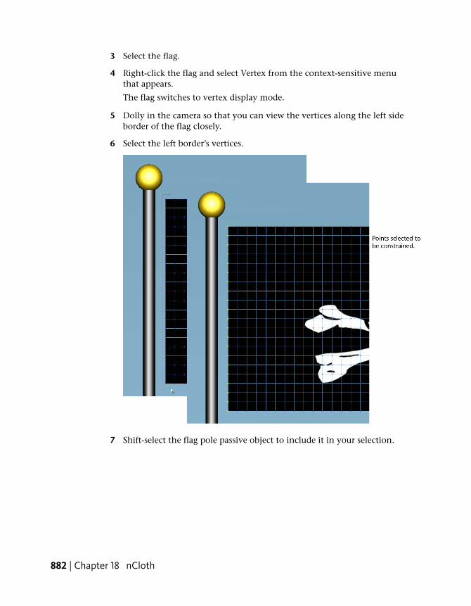
3 Select the flag.
4 Right-click the flag and select Vertex from the context-sensitive menuthat appears.
The flag switches to vertex display mode.
5 Dolly in the camera so that you can view the vertices along the left sideborder of the flag closely.
6 Select the left border’s vertices.
7 Shift-select the flag pole passive object to include it in your selection.
882 | Chapter 18 nCloth

8 Select nConstraint > Point to Surface.
Constraining an nCloth to a passive object | 883

A Point to Surface constraint is created, and constraint links appearbetween the vertices you selected on the nCloth flag, and the surface ofthe flag pole passive object.
884 | Chapter 18 nCloth

9 Play back the flag’s simulation.
The flag gently falls and ripples, but does not continue to fall out of view.This is because the point to Surface nCloth constraint attaching the flagvertices to the flag pole now restricts the position of the whole flag inXYZ space.
Constraining an nCloth to a passive object | 885
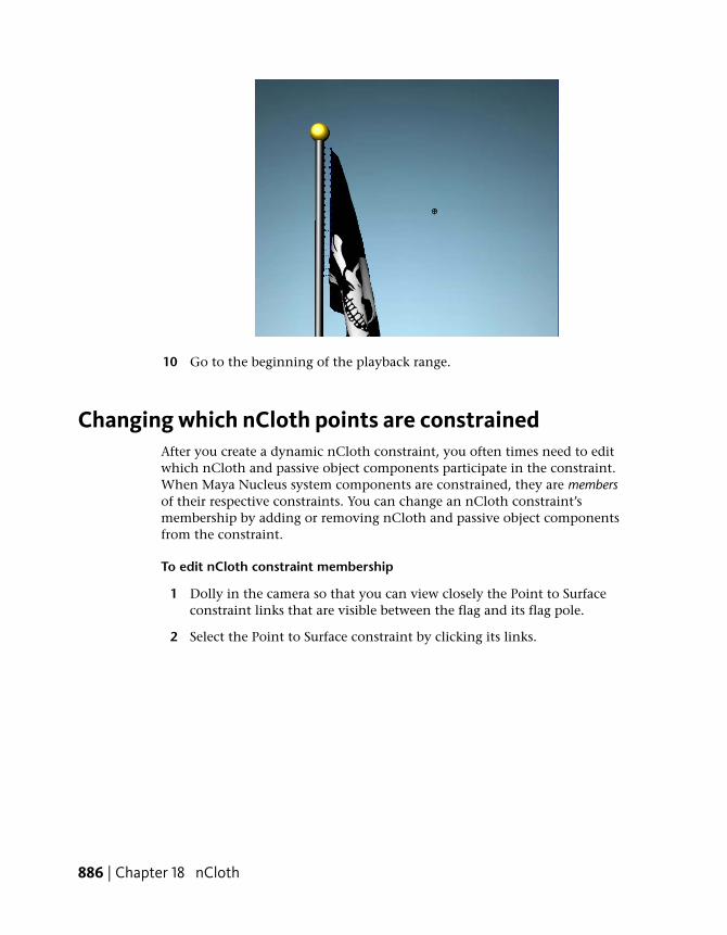
10 Go to the beginning of the playback range.
Changing which nCloth points are constrainedAfter you create a dynamic nCloth constraint, you often times need to editwhich nCloth and passive object components participate in the constraint.When Maya Nucleus system components are constrained, they are membersof their respective constraints. You can change an nCloth constraint’smembership by adding or removing nCloth and passive object componentsfrom the constraint.
To edit nCloth constraint membership
1 Dolly in the camera so that you can view closely the Point to Surfaceconstraint links that are visible between the flag and its flag pole.
2 Select the Point to Surface constraint by clicking its links.
886 | Chapter 18 nCloth

3 Select nConstraint > Select Members.
The flag points and the flag pole surface that are members of the selectedPoint to Surface constraint highlight in the scene view.
Changing which nCloth points are constrained | 887

4 Right-click the flag and select Vertex from the context-sensitive menuthat appears.
The flag switches to vertex display mode.
888 | Chapter 18 nCloth

5 Select all the flag points, except the top most and bottom most points.
Changing which nCloth points are constrained | 889
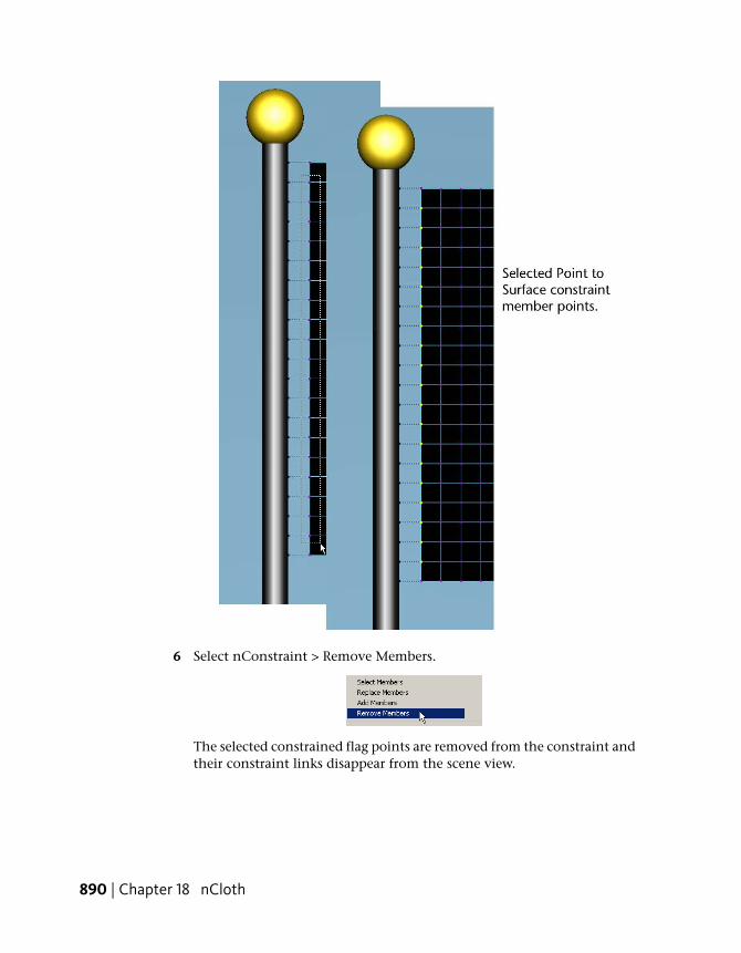
6 Select nConstraint > Remove Members.
The selected constrained flag points are removed from the constraint andtheir constraint links disappear from the scene view.
890 | Chapter 18 nCloth
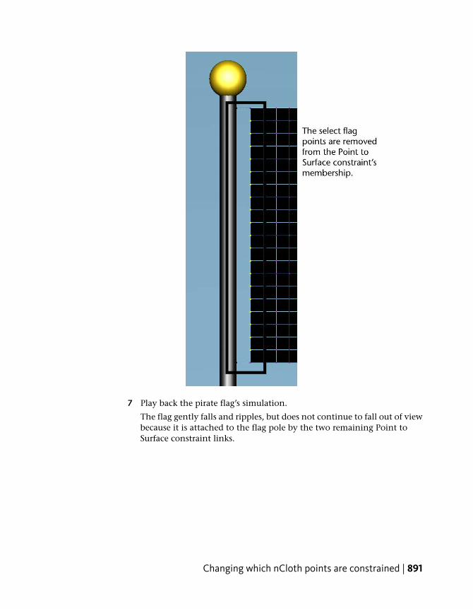
7 Play back the pirate flag’s simulation.
The flag gently falls and ripples, but does not continue to fall out of viewbecause it is attached to the flag pole by the two remaining Point toSurface constraint links.
Changing which nCloth points are constrained | 891
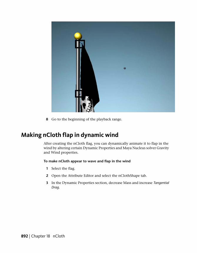
8 Go to the beginning of the playback range.
Making nCloth flap in dynamic windAfter creating the nCloth flag, you can dynamically animate it to flap in thewind by altering certain Dynamic Properties and Maya Nucleus solver Gravityand Wind properties.
To make nCloth appear to wave and flap in the wind
1 Select the flag.
2 Open the Attribute Editor and select the nClothShape tab.
3 In the Dynamic Properties section, decrease Mass and increase TangentialDrag.
892 | Chapter 18 nCloth
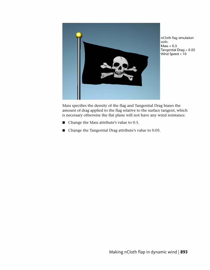
Mass specifies the density of the flag and Tangential Drag biases theamount of drag applied to the flag relative to the surface tangent, whichis necessary otherwise the flat plane will not have any wind resistance.
■ Change the Mass attribute’s value to 0.5.
■ Change the Tangential Drag attribute’s value to 0.05.
Making nCloth flap in dynamic wind | 893

4 Play back the flag’s simulation.
The flag appears lighter, however it still falls.
5 Go to the beginning of the playback range.
6 Select the nucleus tab.
7 In the Gravity and Wind section, increase the Wind Speed.
You can increase the speed at which the flag flaps, as well as the amountof ripples moving across the flag’s surface, by increasing the Maya Nucleussolver’s Wind Speed.
8 Change the Wind Speed attribute’s value to 10.
9 Play back the pirate flag’s simulation.
894 | Chapter 18 nCloth
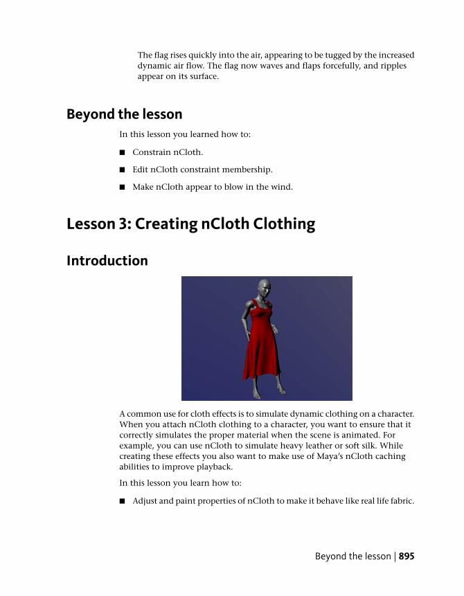
The flag rises quickly into the air, appearing to be tugged by the increaseddynamic air flow. The flag now waves and flaps forcefully, and ripplesappear on its surface.
Beyond the lessonIn this lesson you learned how to:
■ Constrain nCloth.
■ Edit nCloth constraint membership.
■ Make nCloth appear to blow in the wind.
Lesson 3: Creating nCloth Clothing
Introduction
A common use for cloth effects is to simulate dynamic clothing on a character.When you attach nCloth clothing to a character, you want to ensure that itcorrectly simulates the proper material when the scene is animated. Forexample, you can use nCloth to simulate heavy leather or soft silk. Whilecreating these effects you also want to make use of Maya’s nCloth cachingabilities to improve playback.
In this lesson you learn how to:
■ Adjust and paint properties of nCloth to make it behave like real life fabric.
Beyond the lesson | 895
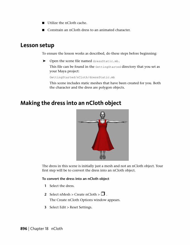
■ Utilize the nCloth cache.
■ Constrain an nCloth dress to an animated character.
Lesson setupTo ensure the lesson works as described, do these steps before beginning:
➤ Open the scene file named dressStatic.mb.
This file can be found in the GettingStarted directory that you set asyour Maya project:
GettingStarted/nCloth/dressStatic.mb
This scene includes static meshes that have been created for you. Boththe character and the dress are polygon objects.
Making the dress into an nCloth object
The dress in this scene is initially just a mesh and not an nCloth object. Yourfirst step will be to convert the dress into an nCloth object.
To convert the dress into an nCloth object
1 Select the dress.
2 Select nMesh > Create nCloth > .
The Create nCloth Options window appears.
3 Select Edit > Reset Settings.
896 | Chapter 18 nCloth
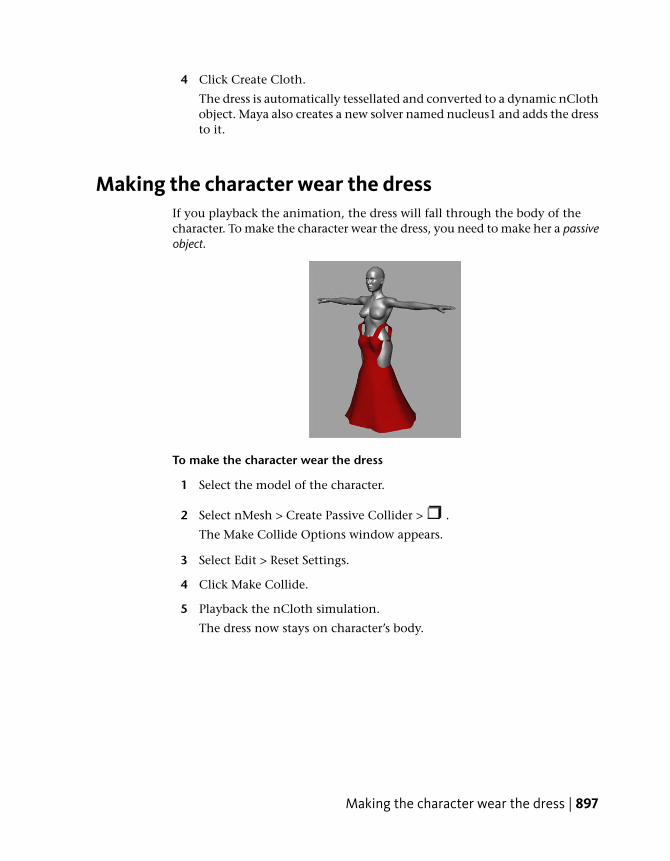
4 Click Create Cloth.
The dress is automatically tessellated and converted to a dynamic nClothobject. Maya also creates a new solver named nucleus1 and adds the dressto it.
Making the character wear the dressIf you playback the animation, the dress will fall through the body of thecharacter. To make the character wear the dress, you need to make her a passiveobject.
To make the character wear the dress
1 Select the model of the character.
2 Select nMesh > Create Passive Collider > .
The Make Collide Options window appears.
3 Select Edit > Reset Settings.
4 Click Make Collide.
5 Playback the nCloth simulation.
The dress now stays on character’s body.
Making the character wear the dress | 897
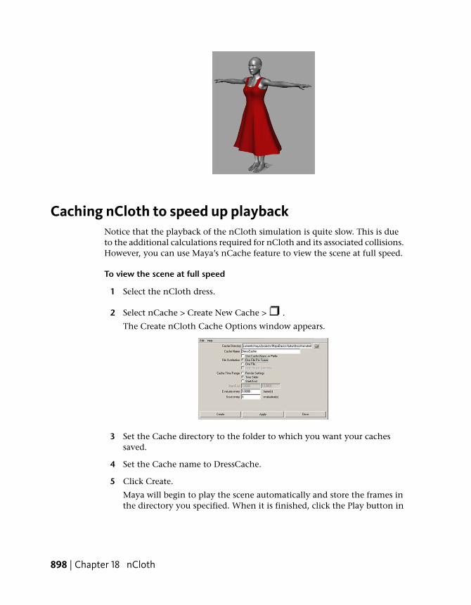
Caching nCloth to speed up playbackNotice that the playback of the nCloth simulation is quite slow. This is dueto the additional calculations required for nCloth and its associated collisions.However, you can use Maya’s nCache feature to view the scene at full speed.
To view the scene at full speed
1 Select the nCloth dress.
2 Select nCache > Create New Cache > .
The Create nCloth Cache Options window appears.
3 Set the Cache directory to the folder to which you want your cachessaved.
4 Set the Cache name to DressCache.
5 Click Create.
Maya will begin to play the scene automatically and store the frames inthe directory you specified. When it is finished, click the Play button in
898 | Chapter 18 nCloth
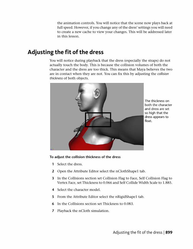
the animation controls. You will notice that the scene now plays back atfull speed. However, if you change any of the dress’ settings you will needto create a new cache to view your changes. This will be addressed laterin this lesson.
Adjusting the fit of the dressYou will notice during playback that the dress (especially the straps) do notactually touch the body. This is because the collision volumes of both thecharacter and the dress are too thick. This means that Maya believes the twoare in contact when they are not. You can fix this by adjusting the collisionthickness of both objects.
To adjust the collision thickness of the dress
1 Select the dress.
2 Open the Attribute Editor select the nClothShape1 tab.
3 In the Collisions section set Collision Flag to Face, Self Collision Flag toVertex Face, set Thickness to 0.066 and Self Collide Width Scale to 1.885.
4 Select the character model.
5 From the Attribute Editor select the nRigidShape1 tab.
6 In the Collisions section set Thickness to 0.083.
7 Playback the nCloth simulation.
Adjusting the fit of the dress | 899

Notice that the simulation appears exactly the same as before. This isbecause you are actually playing your cached simulation. In order to viewyour changes, you will need to make a new cache.
To make a new cache for your nCloth simulation
1 Select the dress.
2 Select nCache > Create New Cache.
Maya automatically plays back the nCloth simulation and saves it to diskas a cache.
3 Playback the scene.
The dress now appears to rest on the character’s skin.
Defining the behavior of nCloth clothingAlthough your dress now fits properly over the character, the dress itself seemsto be made of a very heavy material in a very low gravity environment. Ideally,you want the dress to behave like a light weight material such as silk in agravitational environment similar to our own.
900 | Chapter 18 nCloth
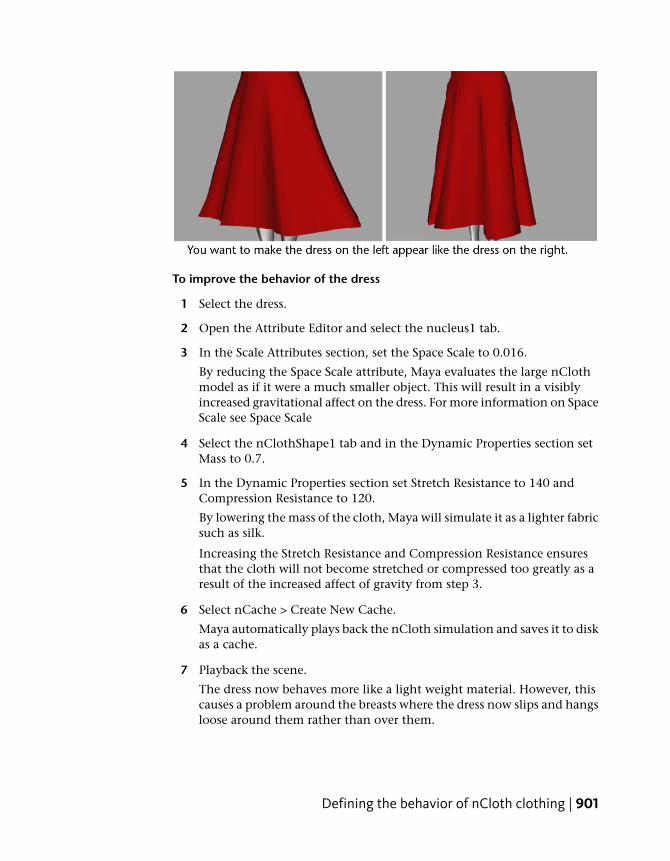
To improve the behavior of the dress
1 Select the dress.
2 Open the Attribute Editor and select the nucleus1 tab.
3 In the Scale Attributes section, set the Space Scale to 0.016.
By reducing the Space Scale attribute, Maya evaluates the large nClothmodel as if it were a much smaller object. This will result in a visiblyincreased gravitational affect on the dress. For more information on SpaceScale see Space Scale
4 Select the nClothShape1 tab and in the Dynamic Properties section setMass to 0.7.
5 In the Dynamic Properties section set Stretch Resistance to 140 andCompression Resistance to 120.
By lowering the mass of the cloth, Maya will simulate it as a lighter fabricsuch as silk.
Increasing the Stretch Resistance and Compression Resistance ensuresthat the cloth will not become stretched or compressed too greatly as aresult of the increased affect of gravity from step 3.
6 Select nCache > Create New Cache.
Maya automatically plays back the nCloth simulation and saves it to diskas a cache.
7 Playback the scene.
The dress now behaves more like a light weight material. However, thiscauses a problem around the breasts where the dress now slips and hangsloose around them rather than over them.
Defining the behavior of nCloth clothing | 901
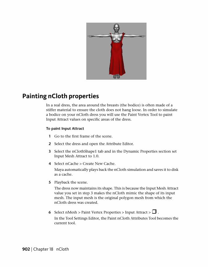
Painting nCloth propertiesIn a real dress, the area around the breasts (the bodice) is often made of astiffer material to ensure the cloth does not hang loose. In order to simulatea bodice on your nCloth dress you will use the Paint Vertex Tool to paintInput Attract values on specific areas of the dress.
To paint Input Attract
1 Go to the first frame of the scene.
2 Select the dress and open the Attribute Editor.
3 Select the nClothShape1 tab and in the Dynamic Properties section setInput Mesh Attract to 1.0.
4 Select nCache > Create New Cache.
Maya automatically plays back the nCloth simulation and saves it to diskas a cache.
5 Playback the scene.
The dress now maintains its shape. This is because the Input Mesh Attractvalue you set in step 3 makes the nCloth mimic the shape of its inputmesh. The input mesh is the original polygon mesh from which thenCloth dress was created.
6 Select nMesh > Paint Vertex Properties > Input Attract > .
In the Tool Settings Editor, the Paint nCloth Attributes Tool becomes thecurrent tool.
902 | Chapter 18 nCloth
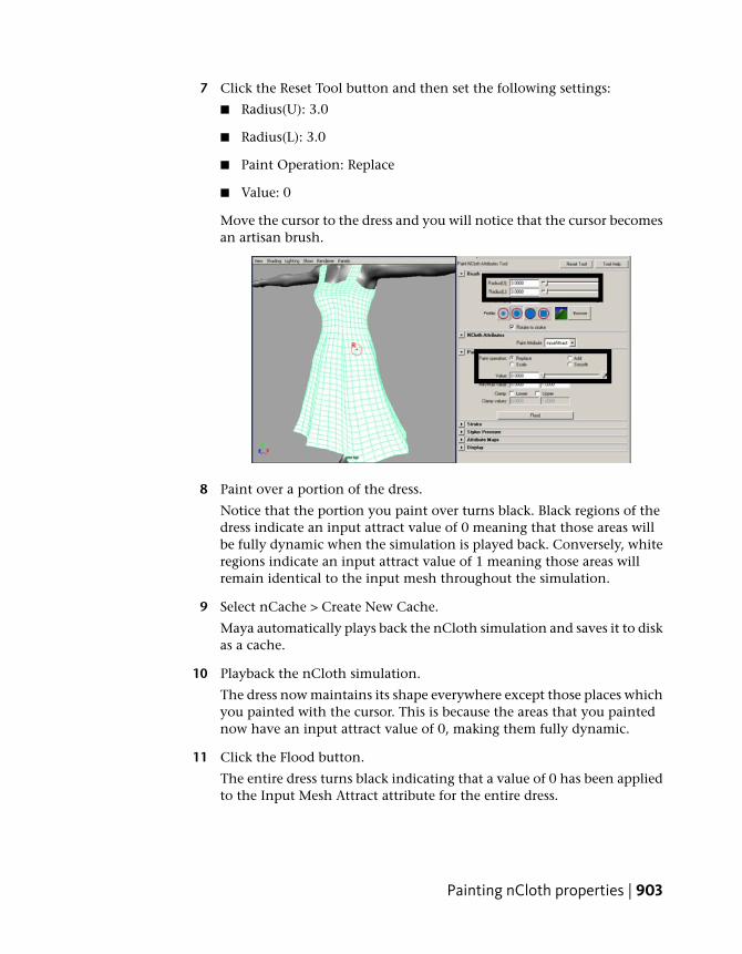
7 Click the Reset Tool button and then set the following settings:
■ Radius(U): 3.0
■ Radius(L): 3.0
■ Paint Operation: Replace
■ Value: 0
Move the cursor to the dress and you will notice that the cursor becomesan artisan brush.
8 Paint over a portion of the dress.
Notice that the portion you paint over turns black. Black regions of thedress indicate an input attract value of 0 meaning that those areas willbe fully dynamic when the simulation is played back. Conversely, whiteregions indicate an input attract value of 1 meaning those areas willremain identical to the input mesh throughout the simulation.
9 Select nCache > Create New Cache.
Maya automatically plays back the nCloth simulation and saves it to diskas a cache.
10 Playback the nCloth simulation.
The dress now maintains its shape everywhere except those places whichyou painted with the cursor. This is because the areas that you paintednow have an input attract value of 0, making them fully dynamic.
11 Click the Flood button.
The entire dress turns black indicating that a value of 0 has been appliedto the Input Mesh Attract attribute for the entire dress.
Painting nCloth properties | 903

12 Set Value to 1.
13 Using the Tool brush, paint around the top of the bodice.
Make sure to dolly and tumble the camera to ensure you have paintedthe entire top of the bodice.
14 Set Value to 0.5.
15 Using the Tool brush, paint the rest of the bodice. Be careful not to paintover your previous values.
16 Dolly and tumble to ensure that you have painted the entire bodice.
17 Select nCache > Create New Cache.
Maya automatically plays back the nCloth simulation and saves it to diskas a cache.
18 Playback the nCloth simulation.
The dress now appears to be made of a light silk, except around the bodicewhere it maintains its shape. If your dress does not appear as the examplebelow, you may need to increase the values painted on your bodice.
904 | Chapter 18 nCloth

This completes the first half of the nCloth clothing lesson. In the second halfof the lesson you will work with an animated character.
Open the second scene for the lessonTo ensure the lesson works as described, do these steps before beginning:
➤ Open the scene file named DressAnimated.mb.
This file can be found in the GettingStarted directory that was installedwith your Maya software:
GettingStarted/nClothDressAnimated.mb
This scene includes an nCloth dress worn by an animated character model.A walk and pose animation is already applied to the character.
Setting the initial stateWhen you load the file you will notice that in the first frame of the animationthe dress is suspended such that it does not touch the character’s body. Thisis because this was the input mesh’s original position. However, for thischaracter you want the dress to be in a relaxed position before the animationbegins. To do this, you need to edit the nCloth’s initial and rest states.
To edit the initial state of the dress.
1 Playback the scene.
Open the second scene for the lesson | 905

The character takes a number of steps from her starting point and thenposes. You will notice however that the dress begins in a suspendedposition and falls onto the character as she walks.
2 Go to the beginning of the playback range.
3 Select the dress.
4 Select nSolver > Initial State > Relax Initial State > .
The Relax Initial State Options window appears.
5 Select Edit > Reset Settings.
6 Set Steps to 300 and then click Relax Initial State.
By setting the Steps option to 300 you are setting the nCloth dress’ initialposition to mimic that of its position at frame 300 of the animation(when the dress has fallen onto the body and relaxes).
906 | Chapter 18 nCloth
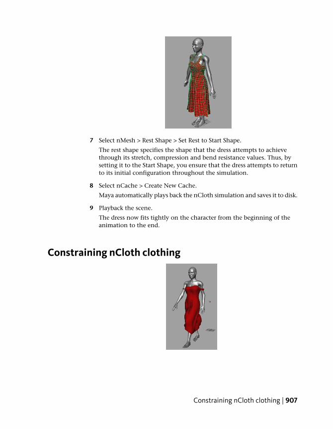
7 Select nMesh > Rest Shape > Set Rest to Start Shape.
The rest shape specifies the shape that the dress attempts to achievethrough its stretch, compression and bend resistance values. Thus, bysetting it to the Start Shape, you ensure that the dress attempts to returnto its initial configuration throughout the simulation.
8 Select nCache > Create New Cache.
Maya automatically plays back the nCloth simulation and saves it to disk.
9 Playback the scene.
The dress now fits tightly on the character from the beginning of theanimation to the end.
Constraining nCloth clothing
Constraining nCloth clothing | 907
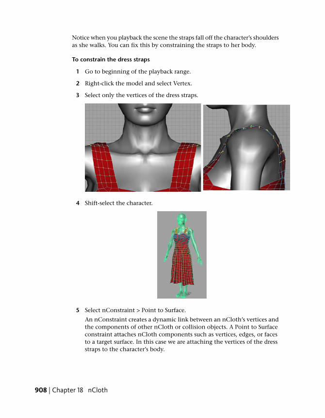
Notice when you playback the scene the straps fall off the character’s shouldersas she walks. You can fix this by constraining the straps to her body.
To constrain the dress straps
1 Go to beginning of the playback range.
2 Right-click the model and select Vertex.
3 Select only the vertices of the dress straps.
4 Shift-select the character.
5 Select nConstraint > Point to Surface.
An nConstraint creates a dynamic link between an nCloth’s vertices andthe components of other nCloth or collision objects. A Point to Surfaceconstraint attaches nCloth components such as vertices, edges, or facesto a target surface. In this case we are attaching the vertices of the dressstraps to the character’s body.
908 | Chapter 18 nCloth
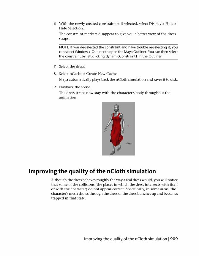
6 With the newly created constraint still selected, select Display > Hide >Hide Selection.
The constraint markers disappear to give you a better view of the dressstraps.
NOTE If you de-selected the constraint and have trouble re-selecting it, youcan select Window > Outliner to open the Maya Outliner. You can then selectthe constraint by left-clicking dynamicConstraint1 in the Outliner.
7 Select the dress.
8 Select nCache > Create New Cache.
Maya automatically plays back the nCloth simulation and saves it to disk.
9 Playback the scene.
The dress straps now stay with the character’s body throughout theanimation.
Improving the quality of the nCloth simulationAlthough the dress behaves roughly the way a real dress would, you will noticethat some of the collisions (the places in which the dress intersects with itselfor with the character) do not appear correct. Specifically, in some areas, thecharacter’s mesh shows through the dress or the dress bunches up and becomestrapped in that state.
Improving the quality of the nCloth simulation | 909
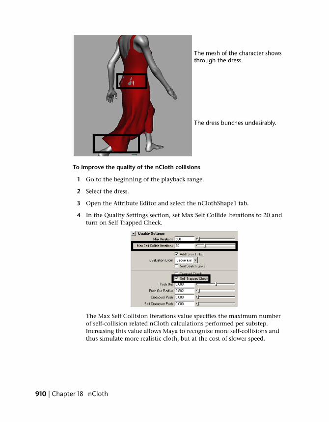
To improve the quality of the nCloth collisions
1 Go to the beginning of the playback range.
2 Select the dress.
3 Open the Attribute Editor and select the nClothShape1 tab.
4 In the Quality Settings section, set Max Self Collide Iterations to 20 andturn on Self Trapped Check.
The Max Self Collision Iterations value specifies the maximum numberof self-collision related nCloth calculations performed per substep.Increasing this value allows Maya to recognize more self-collisions andthus simulate more realistic cloth, but at the cost of slower speed.
910 | Chapter 18 nCloth
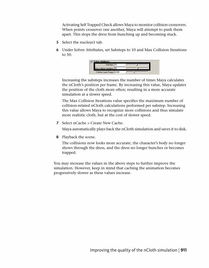
Activating Self Trapped Check allows Maya to monitor collision crossovers.When points crossover one another, Maya will attempt to push themapart. This stops the dress from bunching up and becoming stuck.
5 Select the nucleus1 tab.
6 Under Solver Attributes, set Substeps to 10 and Max Collision Iterationsto 50.
Increasing the substeps increases the number of times Maya calculatesthe nCloth’s position per frame. By increasing this value, Maya updatesthe position of the cloth more often; resulting in a more accuratesimulation at a slower speed.
The Max Collision Iterations value specifies the maximum number ofcollision-related nCloth calculations performed per substep. Increasingthis value allows Maya to recognize more collisions and thus simulatemore realistic cloth, but at the cost of slower speed.
7 Select nCache > Create New Cache.
Maya automatically plays back the nCloth simulation and saves it to disk.
8 Playback the scene.
The collisions now looks more accurate, the character’s body no longershows through the dress, and the dress no longer bunches or becomestrapped.
You may increase the values in the above steps to further improve thesimulation. However, keep in mind that caching the animation becomesprogressively slower as these values increase.
Improving the quality of the nCloth simulation | 911

Smoothing nCloth clothingTo improve the quality and overall look of the dress you can perform a polygonsmooth. Polygon smoothing will increase the number of polygons in yournCloth mesh to give it a smoother overall appearance.
To smooth the dress
1 Select the dress and in the Polygons menu set select Mesh > Smooth.
2 Return to the nDynamics menu set.
3 Select nCache > Create New Cache.
Maya automatically plays back the nCloth simulation and saves it to disk.
4 Playback the scene.
The dress in the final animation is smoothed giving it a much silkierappearance.
912 | Chapter 18 nCloth
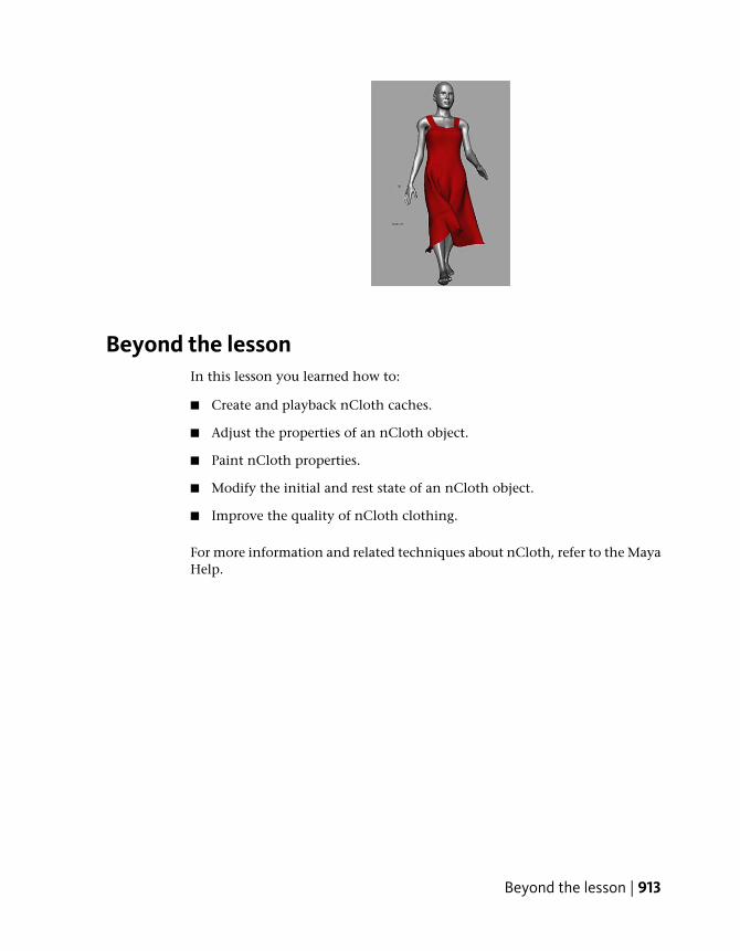
Beyond the lessonIn this lesson you learned how to:
■ Create and playback nCloth caches.
■ Adjust the properties of an nCloth object.
■ Paint nCloth properties.
■ Modify the initial and rest state of an nCloth object.
■ Improve the quality of nCloth clothing.
For more information and related techniques about nCloth, refer to the MayaHelp.
Beyond the lesson | 913

914
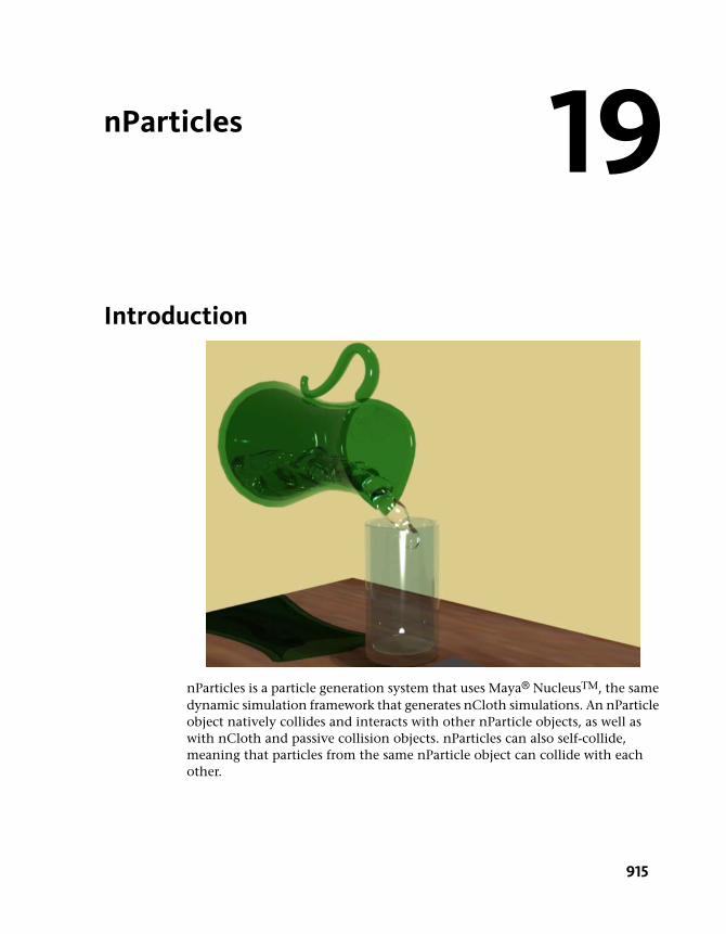
nParticles
Introduction
nParticles is a particle generation system that uses Maya® NucleusTM, the samedynamic simulation framework that generates nCloth simulations. An nParticleobject natively collides and interacts with other nParticle objects, as well aswith nCloth and passive collision objects. nParticles can also self-collide,meaning that particles from the same nParticle object can collide with eachother.
19
915
Nucleus dynamics allows you to create particle effects and dynamic simulationsthat cannot be achieved with Maya classic particles. For example, you can useLiquid Simulation attributes to create particle systems that behave like liquids.You can also create effects in which particles interact and drive nClothanimations and deformations.
This chapter includes these tutorials:
■ Lesson 1: Creating nParticles on page 917
■ Lesson 2: Creating a smoke simulation with nParticles on page 930
■ Lesson 3: Creating a liquid simulation with nParticles on page 953
Preparing for the tutorialsTo ensure the lessons work as described, do these steps before beginning:
1 Make sure you understand the basic concepts of polygon modeling,animation, and dynamics.
2 If you have not already done so, copy the GettingStarted folder fromits installation location to your projects directory. Then, set theGettingStarted directory as your Maya project. For more information,see Copying and setting the Maya project on page 25 in the GettingStarted with Maya guide.
3 Select the nDynamics menu set. Unless otherwise noted, the directionsin this chapter for making menu selections assume you’ve already selectedthe nDynamics menu set.
916 | Chapter 19 nParticles

Lesson 1: Creating nParticles
Introduction
In this lesson, you will be introduced to the basic concepts of Nucleusdynamics, as well as learn how to create an nParticle and emitter object. Youwill then adjust nParticle object attributes to create a simple nParticle effect.In this lesson, you also learn how to:
■ Create passive collision objects for your nParticles to collide with.
■ Set nParticle size.
■ Adjust Nucleus node attributes.
■ Adjust attributes to control the behavior of your nParticles.
Lesson 1: Creating nParticles | 917

Lesson setupTo ensure this lesson works as described, open the scene file namednParticle_Candy.mb. This file is in the GettingStarted directory that you setas your Maya project:
GettingStarted/nParticles/nParticle_Candy.mb
This scene includes textured polygon models including a desk, bowl, andcandy package.
Creating an nParticle systemBefore creating an nParticle system, you must decide which nParticle styleand creation method suits your nParticle effect. In this lesson, nParticles areused to simulate candies that are poured from a package into a bowl.
To achieve the appropriate look and behavior, you will use Ball style nParticles.nParticle styles are like templates that provide preset attribute settings for thenParticle object's appearance, size, render type, and collision properties. Tocreate the nParticle system, you will emit nParticles from the surface of apolygon plane that is located inside the candy package.
To create an nParticle system
1 Select nParticles > Create nParticles > Balls.
2 In the Outliner, select candy_emitter_surface, then select nParticles > Create
nParticles > Emit from Object > .
918 | Chapter 19 nParticles
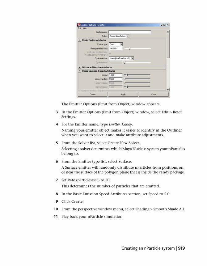
The Emitter Options (Emit from Object) window appears.
3 In the Emitter Options (Emit from Object) window, select Edit > ResetSettings.
4 For the Emitter name, type Emitter_Candy.
Naming your emitter object makes it easier to identify in the Outlinerwhen you want to select it and make attribute adjustments.
5 From the Solver list, select Create New Solver.
Selecting a solver determines which Maya Nucleus system your nParticlesbelong to.
6 From the Emitter type list, select Surface.
A Surface emitter will randomly distribute nParticles from positions onor near the surface of the polygon plane that is inside the candy package.
7 Set Rate (particles/sec) to 50.
This determines the number of particles that are emitted.
8 In the Basic Emission Speed Attributes section, set Speed to 5.0.
9 Click Create.
10 From the perspective window menu, select Shading > Smooth Shade All.
11 Play back your nParticle simulation.
Creating an nParticle system | 919

nParticles are emitted, but they fall through the side of the candy packageand disappear. This is because the nParticles cannot yet collide with anyof the other objects in your scene. For your nParticles to collide with thecandy package and bowl, these meshes need to be passive collision objectsand members of the same Maya Nucleus solver system as the nParticles.
Making nParticles collide with their environmentIn the second step of creating an nParticle effect, you convert the meshes youwant the nParticles to collide with to passive collision objects. When nParticlescollide with passive collision objects, their behavior, speed, and directionchange. Passive collision objects are not affected by collisions with otherobjects.
In this lesson, you convert the candy package, bowl, and the desk surfacegeometry to passive collision objects. The nParticles can then collide withthese objects.
To convert geometry to passive collision objects
1 Rewind the simulation to the start frame.
2 In the scene view, Shift-select the package and bowl meshes as well asthe surface of the desk.
3 Select nMesh > Create Passive Collider > .
920 | Chapter 19 nParticles
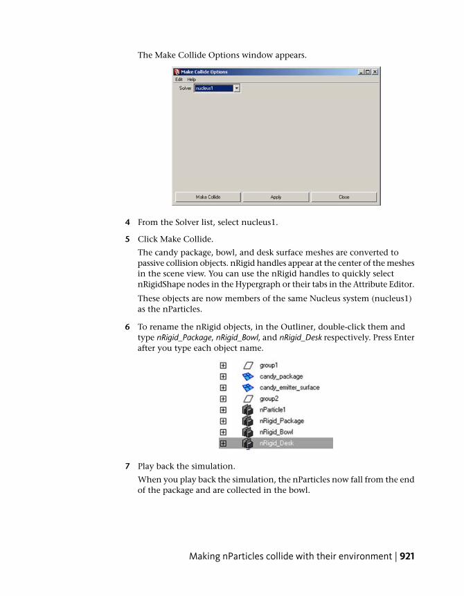
The Make Collide Options window appears.
4 From the Solver list, select nucleus1.
5 Click Make Collide.
The candy package, bowl, and desk surface meshes are converted topassive collision objects. nRigid handles appear at the center of the meshesin the scene view. You can use the nRigid handles to quickly selectnRigidShape nodes in the Hypergraph or their tabs in the Attribute Editor.
These objects are now members of the same Nucleus system (nucleus1)as the nParticles.
6 To rename the nRigid objects, in the Outliner, double-click them andtype nRigid_Package, nRigid_Bowl, and nRigid_Desk respectively. Press Enterafter you type each object name.
7 Play back the simulation.
When you play back the simulation, the nParticles now fall from the endof the package and are collected in the bowl.
Making nParticles collide with their environment | 921
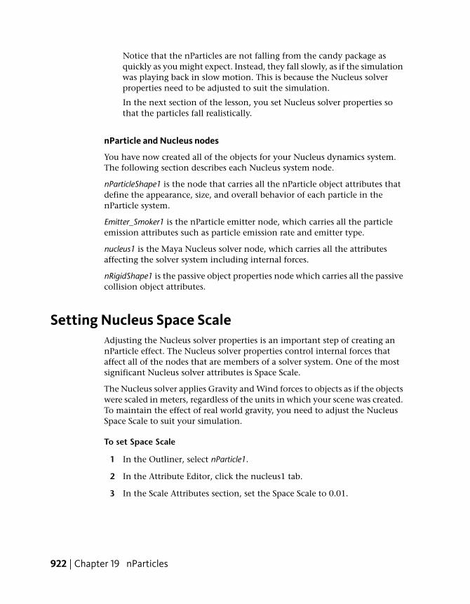
Notice that the nParticles are not falling from the candy package asquickly as you might expect. Instead, they fall slowly, as if the simulationwas playing back in slow motion. This is because the Nucleus solverproperties need to be adjusted to suit the simulation.
In the next section of the lesson, you set Nucleus solver properties sothat the particles fall realistically.
nParticle and Nucleus nodes
You have now created all of the objects for your Nucleus dynamics system.The following section describes each Nucleus system node.
nParticleShape1 is the node that carries all the nParticle object attributes thatdefine the appearance, size, and overall behavior of each particle in thenParticle system.
Emitter_Smoker1 is the nParticle emitter node, which carries all the particleemission attributes such as particle emission rate and emitter type.
nucleus1 is the Maya Nucleus solver node, which carries all the attributesaffecting the solver system including internal forces.
nRigidShape1 is the passive object properties node which carries all the passivecollision object attributes.
Setting Nucleus Space ScaleAdjusting the Nucleus solver properties is an important step of creating annParticle effect. The Nucleus solver properties control internal forces thataffect all of the nodes that are members of a solver system. One of the mostsignificant Nucleus solver attributes is Space Scale.
The Nucleus solver applies Gravity and Wind forces to objects as if the objectswere scaled in meters, regardless of the units in which your scene was created.To maintain the effect of real world gravity, you need to adjust the NucleusSpace Scale to suit your simulation.
To set Space Scale
1 In the Outliner, select nParticle1.
2 In the Attribute Editor, click the nucleus1 tab.
3 In the Scale Attributes section, set the Space Scale to 0.01.
922 | Chapter 19 nParticles
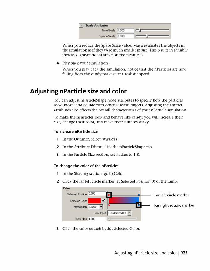
When you reduce the Space Scale value, Maya evaluates the objects inthe simulation as if they were much smaller in size. This results in a visiblyincreased gravitational affect on the nParticles.
4 Play back your simulation.
When you play back the simulation, notice that the nParticles are nowfalling from the candy package at a realistic speed.
Adjusting nParticle size and colorYou can adjust nParticleShape node attributes to specify how the particleslook, move, and collide with other Nucleus objects. Adjusting the emitterattributes also affects the overall characteristics of your nParticle simulation.
To make the nParticles look and behave like candy, you will increase theirsize, change their color, and make their surfaces sticky.
To increase nParticle size
1 In the Outliner, select nParticle1.
2 In the Attribute Editor, click the nParticleShape tab.
3 In the Particle Size section, set Radius to 1.8.
To change the color of the nParticles
1 In the Shading section, go to Color.
2 Click the far left circle marker (at Selected Position 0) of the ramp.
3 Click the color swatch beside Selected Color.
Adjusting nParticle size and color | 923
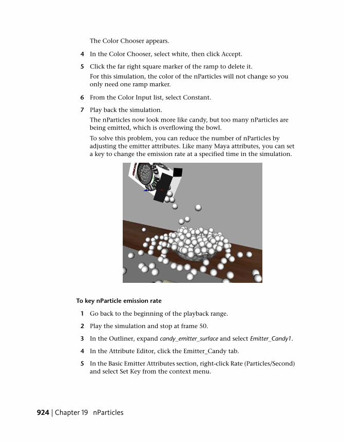
The Color Chooser appears.
4 In the Color Chooser, select white, then click Accept.
5 Click the far right square marker of the ramp to delete it.
For this simulation, the color of the nParticles will not change so youonly need one ramp marker.
6 From the Color Input list, select Constant.
7 Play back the simulation.
The nParticles now look more like candy, but too many nParticles arebeing emitted, which is overflowing the bowl.
To solve this problem, you can reduce the number of nParticles byadjusting the emitter attributes. Like many Maya attributes, you can seta key to change the emission rate at a specified time in the simulation.
To key nParticle emission rate
1 Go back to the beginning of the playback range.
2 Play the simulation and stop at frame 50.
3 In the Outliner, expand candy_emitter_surface and select Emitter_Candy1.
4 In the Attribute Editor, click the Emitter_Candy tab.
5 In the Basic Emitter Attributes section, right-click Rate (Particles/Second)and select Set Key from the context menu.
924 | Chapter 19 nParticles

A key is created with the nParticle emission rate set at 50.
6 Play the simulation for five more frames to frame 55.
7 Set Rate (Particles/Second) to 0.
8 Right-click Rate (Particles/Second) and select Set Key from the contextmenu.
A key is created with the nParticle emission rate set at 0.
9 Go back to the beginning of the playback range and play the simulation.
nParticles are now emitted until frame 55.
Adjusting nParticle collision attributesnParticle Collisions attributes determine the behavior of nParticles when theycollide each other and with other Nucleus objects. In this section of the lesson,you make the nParticles sticky like candy by adjusting the Friction andStickiness attributes.
To adjust nParticle Collisions attributes
1 In the Outliner, select nParticle1.
2 In the Attribute Editor, click the nParticleShape tab.
3 In the Collisions section, set the following:
■ Bounce: 0
■ Friction: 0.2
■ Stickiness: 0.5
4 Play back your simulation.
5 Notice that the nParticles are now sticking each other and piling up atthe edge of the bowl.
Friction and Stickiness are similar attributes in that Friction is a forceacting in the tangent direction, while Stickiness is an adhesion force inthe normal direction. When Nucleus objects collide, the affect of theirFriction and Stickiness values are additive. For example, if the Stickinessvalue of the nParticles and the bowl are 0.5, the overall Stickiness actingon both objects is equal to 1.0.
Adjusting nParticle collision attributes | 925
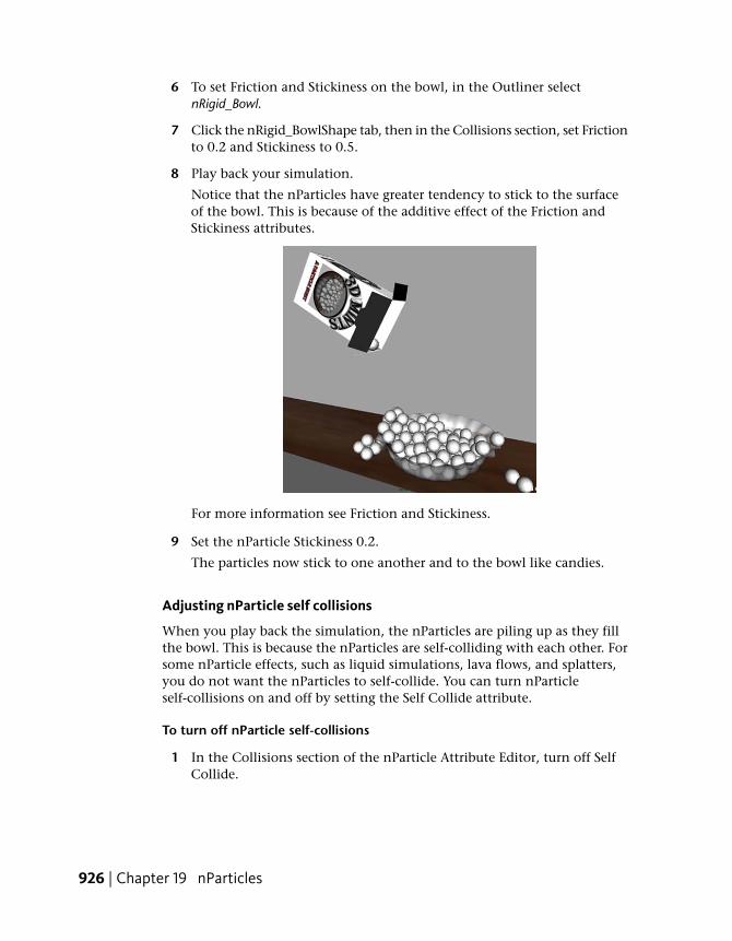
6 To set Friction and Stickiness on the bowl, in the Outliner selectnRigid_Bowl.
7 Click the nRigid_BowlShape tab, then in the Collisions section, set Frictionto 0.2 and Stickiness to 0.5.
8 Play back your simulation.
Notice that the nParticles have greater tendency to stick to the surfaceof the bowl. This is because of the additive effect of the Friction andStickiness attributes.
For more information see Friction and Stickiness.
9 Set the nParticle Stickiness 0.2.
The particles now stick to one another and to the bowl like candies.
Adjusting nParticle self collisions
When you play back the simulation, the nParticles are piling up as they fillthe bowl. This is because the nParticles are self-colliding with each other. Forsome nParticle effects, such as liquid simulations, lava flows, and splatters,you do not want the nParticles to self-collide. You can turn nParticleself-collisions on and off by setting the Self Collide attribute.
To turn off nParticle self-collisions
1 In the Collisions section of the nParticle Attribute Editor, turn off SelfCollide.
926 | Chapter 19 nParticles

2 Play back your simulation.
Notice that the nParticles no longer pile up, but blend and overlap witheach other.
Each nParticle has an outer boundary that determines the distancebetween the nParticle and an object at collision. The Collide Width Scaleattribute sets the collision distance between the nParticles and otherNucleus objects. The Self Collide Width Scale attribute sets the collisiondistance between self-colliding nParticles.
By default, Collide Width Scale and Self Collide Width Scale are set to 1for normal collisions. Turning off Self Collide is like setting the Self CollideWidth Scale to 0.
3 Turn on Self Collide, and set Self Collide Width Scale to 1.5.
4 Play back the simulation.
Notice that the nParticles appear to collide with each other when theyfill the bowl, but they don't touch one another. The gaps between thenParticles are due to the increased Self Collide Width Scale.
Adjusting nParticle collision attributes | 927

In the next step, you will display the current Self Collision Width Scaleby turning on the Solver Display.
5 From the Solver Display list, select Self Collision Thickness.
The nParticles now appear with their Self Collision Thickness displayedin yellow. You can make adjustments to the Self Collide Width Scale andsee how the thickness affects the space between colliding nParticles.
6 Set Self Collide Width Scale back to 1.0, and the Solver Display to Off.
7 Play back the simulation.
928 | Chapter 19 nParticles
Beyond the lessonIn this lesson you were introduced to the basic concepts of nParticles and theNucleus dynamics system. In addition, you learned how to:
■ Create nParticles by emitting them from a polygon object using a Surfacetype particle emitter.
■ Set the size of the nParticles using the Radius attribute.
■ Set the color of you nParticles.
■ Set nParticle Collisions attributes to control the behavior of nParticles.
■ Turn off nParticle self-collisions.
■ Set the collision distance between self-colliding nParticles by setting SelfCollide Width Scale.
For more information and related techniques about nParticles, refer to theMaya Help.
Beyond the lesson | 929

Lesson 2: Creating a smoke simulation withnParticles
Introduction
For the smoke simulation in this lesson, you create an nParticle systemcomposed of an nParticle object, an emitter object, and a nucleus node. Youwill add a Volume Axis field to your effect to create turbulence and swirlingin the nParticle smoke. This field helps create the realistic behavior of smokeas it cools, rises and dissipates. To finish your smoke simulation, you will alsoadd a Nucleus Wind force to make the smoke drift as it disappears.
Lesson setupTo ensure this lesson works as described, open the scene file namedSmoke_Simulation_1.mb. This file is in the GettingStarted directory that youset as your Maya project:
GettingStarted/nParticles/Smoke_Simulation_1.mb
930 | Chapter 19 nParticles

This scene includes textured polygon models including a desk, ashtray, andcigarette.
Creating an nParticle systemIn this part of this lesson, you create an nParticle object and its emitter object.An emitter controls the position, direction, quantity and initial velocity ofthe emitted nParticles when they are born (emitted into the scene).
Creating an nParticle and emitter object
To create an nParticle and emitter objects
1 Select nParticles > Create nParticles > Cloud.
Selecting Cloud presets some nParticleShape attributes that are suitablefor simulations such as smoke, dust, or fog.
Creating an nParticle system | 931

2 To create an nParticle emitter object, select nParticles > Create nParticles
> Create Emitter > .
The Emitter Options (Create) window appears.
3 In the Emitter Options (Create) window, select Edit > Reset Settings.
4 In the Emitter name field, type Emitter_Smoke.
Naming your emitter object makes it easier to identify in the Outlinerwhen you want to select it and make attribute adjustments.
5 From the Solver list, select Create New Solver.
Selecting a solver determines which Maya Nucleus system your nParticlesbelong to.
6 In the Basic Emitter Attributes section, set the following:
■ Emitter type: Directional.
■ Rate (particles/sec): 120This sets the number of particles that are emitted into the scene. Thehigher the emission rate the thicker the smoke appears.
7 In the Basic Emission Speed Attributes section, set the following:
■ Speed: 2.5.
■ Speed random: 5.0.
932 | Chapter 19 nParticles

When Speed random is set to a positive value, the emitter generatesrandom speeds for each nParticle.
8 Click Create.
An Emitter_Smoke1, nParticleShape1, and a nucleus1 node appear in theAttribute Editor.
9 To rename the nParticle object, in the Outliner, double-click nParticle1and type nParticle_Smoke then press Enter.
Renaming your nParticle object makes it easier to identify when you havemore than one in your scene.
Moving the nParticle emitter
When you create an nParticle and emitter objects, they are placed at the sceneorigin. For this lesson, you need to move the emitter so that the particles areemitted near the tip of the cigarette.
To move the nParticle emitter object
1 In the Outliner, select the Emitter_Smoke1 object.
2 Display the Channel Box by clicking .
3 In the Channel Box enter the following values:
■ Translate X: 49.3
■ Translate Y: 121
■ Translate Z: -27.3
4 In the scene view, dolly and tumble so that you get a close-up view ofthe cigarette.
The nParticle emitter is now positioned near the tip of the cigarette.
Creating an nParticle system | 933
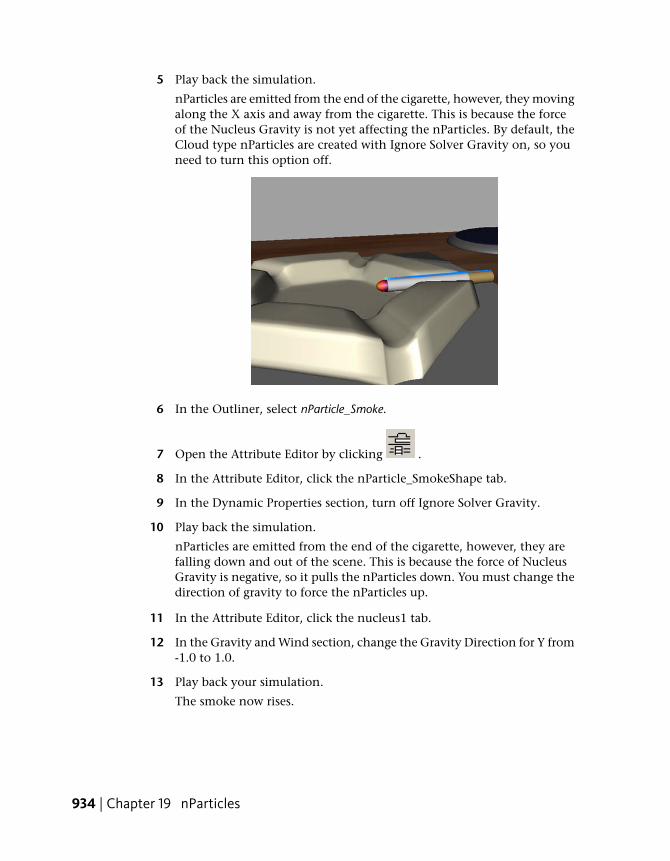
5 Play back the simulation.
nParticles are emitted from the end of the cigarette, however, they movingalong the X axis and away from the cigarette. This is because the forceof the Nucleus Gravity is not yet affecting the nParticles. By default, theCloud type nParticles are created with Ignore Solver Gravity on, so youneed to turn this option off.
6 In the Outliner, select nParticle_Smoke.
7 Open the Attribute Editor by clicking .
8 In the Attribute Editor, click the nParticle_SmokeShape tab.
9 In the Dynamic Properties section, turn off Ignore Solver Gravity.
10 Play back the simulation.
nParticles are emitted from the end of the cigarette, however, they arefalling down and out of the scene. This is because the force of NucleusGravity is negative, so it pulls the nParticles down. You must change thedirection of gravity to force the nParticles up.
11 In the Attribute Editor, click the nucleus1 tab.
12 In the Gravity and Wind section, change the Gravity Direction for Y from-1.0 to 1.0.
13 Play back your simulation.
The smoke now rises.
934 | Chapter 19 nParticles
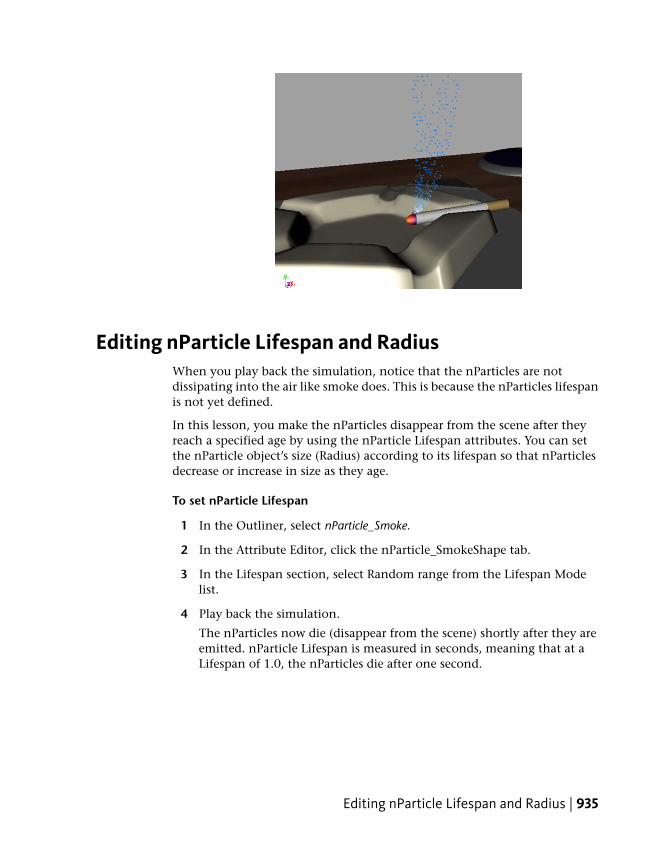
Editing nParticle Lifespan and RadiusWhen you play back the simulation, notice that the nParticles are notdissipating into the air like smoke does. This is because the nParticles lifespanis not yet defined.
In this lesson, you make the nParticles disappear from the scene after theyreach a specified age by using the nParticle Lifespan attributes. You can setthe nParticle object’s size (Radius) according to its lifespan so that nParticlesdecrease or increase in size as they age.
To set nParticle Lifespan
1 In the Outliner, select nParticle_Smoke.
2 In the Attribute Editor, click the nParticle_SmokeShape tab.
3 In the Lifespan section, select Random range from the Lifespan Modelist.
4 Play back the simulation.
The nParticles now die (disappear from the scene) shortly after they areemitted. nParticle Lifespan is measured in seconds, meaning that at aLifespan of 1.0, the nParticles die after one second.
Editing nParticle Lifespan and Radius | 935

5 Set Lifespan to 5.
6 To add some randomization to the nParticle’s lifespan, set LifespanRandom to 5.
7 Rewind the simulation and play it back.
The nParticles die off more randomly, but the nParticle object is still notdense enough to look like smoke. You can make your nParticle objectdenser by increasing the nParticle Radius.
936 | Chapter 19 nParticles

For a realistic smoke simulation, the nParticles must gradually disperse as theyrise in the air. You can use the Radius Scale ramp to increase the radius ofnParticles as they age, which creates the effect of smoke dispersing until itgradually disappears.
To set nParticle size
1 In the Particle Size section, set Radius to 5.0.
2 In the Radius Scale section, select the first marker in the ramp, set SelectedPosition to 0.016, and set Selected Value to 0.04.
Creating a new marker allows you to set two Selected Value and SelectedPosition values. Each Selected Value specifies a scaling value for thenParticle object's Radius attribute. By default, ramps define a scaling valueof 1, meaning that only one mark exists on the ramp and that marker
Editing nParticle Lifespan and Radius | 937

represents an attribute scaling factor of 1. Setting a selected position to0.5 sets per-particle radius to half the Radius value.
3 Click in the ramp to create additional markers and set the SelectedPosition and Selected Value for the new markers to the following values:
SelectedValue
Selected Posi-tion
Marker
0.1800.7322
0.4800.8823
1.01.04
For each point in the ramp, leave Interpolation at its default setting ofLinear.
4 To map nParticle Radius to the nParticles’ age, set Radius Scale Input toNormalized Age.
When Normalized Age is used, per-particle radius is mapped within therange of the nParticle object’s lifespan.
5 To add randomization to the per-particle radius, set Radius ScaleRandomize to 0.25.
6 Play back the simulation.
You can continue to adjust the per-particle radius by adding more markersto the ramp, or optimize the ramp values as the simulation plays back.
938 | Chapter 19 nParticles
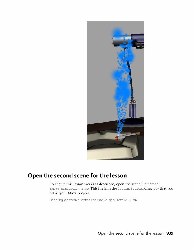
Open the second scene for the lessonTo ensure this lesson works as described, open the scene file namedSmoke_Simulation_2.mb. This file is in the GettingStarted directory that youset as your Maya project:
GettingStarted/nParticles/Smoke_Simulation_2.mb
Open the second scene for the lesson | 939
Adding a Volume Axis fieldYou can use Maya Fields to animate the motion of nParticles and create theeffect of nParticles flowing around obstacles, as well as creating plumingsmoke, swirling tornadoes, and rocket exhaust. For a smoke simulation, youcan add a Volume Axis field to the scene to create turbulence and swirlingeffects in the smoke as it rises through the air.
Maya Fields are not part of an nParticle object's Nucleus system and thereforeyou may need to compensate for the force of Nucleus Gravity and Wind byincreasing or decreasing the field's magnitude. Depending on the effect youare creating, you can also turn on Ignore Solver Gravity or Ignore Solver Windon the nParticleShape node so that your nParticle object is only affected byMaya Fields. For more information about Maya fields see the Dynamics guide.
To create a Volume Axis field
1 In the Outliner, select nParticle_Smoke, then add a Volume Axis field by
selecting Fields > Volume Axis > .
The Volume Axis Options window appears.
2 In the Volume Axis Options window, select Edit > Reset Settings.
3 In Volume axis field name, type Field_Smoke.
4 Set the following Volume Axis field settings:
■ Magnitude: 90
■ Attenuation: 2.0
■ Volume Shape: Cube
■ Away From Center: 4.546
■ Directional Speed: 1.834
■ Direction: X to 0 and Y to 1.0.
■ Turbulence: 0.661
■ Turbulence Speed: 0.157
5 Click Create.
A Field_Smoke1 node appears in the Attribute Editor and in the Outliner.
940 | Chapter 19 nParticles

The Volume Axis field is placed at the scene origin by default. You mustreposition the field so that the emitted nParticles travel through thevolume.
To position the field in the path of the emitted nParticles
1 In the Outliner, select Field_Smoke1 and open the Channel Box by clicking
.
2 In the Channel Box under Field_Smoke1, set the following:
■ TranslateX: 49.57
■ TranslateY: 133.8
■ TranslateZ: -26.49
■ ScaleX: 10
■ ScaleY: 10
■ ScaleZ: 10
3 Play the simulation.
Adding a Volume Axis field | 941

The field creates turbulence in the nParticle smoke as it rises.
However, to create the effect of the smoke curling and dissipating, youneed to adjust the field and nParticle attributes further. For example, theemitted nParticles have too much velocity for the field to influence theirbehavior. You will make these adjustments in the next section.
Adjusting nParticle velocityWhen using Maya Fields with emitted nParticles, some particles move tooquickly through the field to produce the desired effect. You can control howmuch of an nParticle object's velocity is retained from frame to frame byadjusting the Conserve attribute. You can further control the velocity of theparticles as they enter the Volume Axis field by increasing the nParticle object’sDrag. Drag adds friction between the air and nParticles, which slows theparticles down.
To adjust nParticle velocity for the field
1 In the Outliner, select nParticle_Smoke.
2 Open the Attribute Editor by clicking .
3 In the Dynamic Properties section of the nParticle_SmokeShape AttributeEditor, set Conserve to 0.05 and Drag to 0.149.
942 | Chapter 19 nParticles
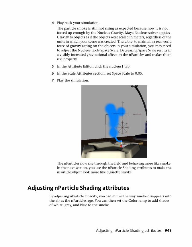
4 Play back your simulation.
The particle smoke is still not rising as expected because now it is notforced up enough by the Nucleus Gravity. Maya Nucleus solver appliesGravity to objects as if the objects were scaled in meters, regardless of theunits in which your scene was created. Therefore, to maintain a real worldforce of gravity acting on the objects in your simulation, you may needto adjust the Nucleus node Space Scale. Decreasing Space Scale results ina visibly increased gravitational affect on the nParticles and makes themrise properly.
5 In the Attribute Editor, click the nucleus1 tab.
6 In the Scale Attributes section, set Space Scale to 0.05.
7 Play the simulation.
The nParticles now rise through the field and behaving more like smoke.In the next section, you use the nParticle Shading attributes to make thenParticle object look more like cigarette smoke.
Adjusting nParticle Shading attributesBy adjusting nParticle Opacity, you can mimic the way smoke disappears intothe air as the nParticles age. You can then set the Color ramp to add shadesof white, gray, and blue to the smoke.
Adjusting nParticle Shading attributes | 943
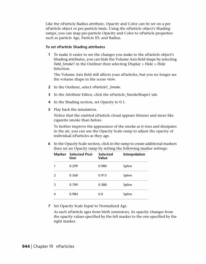
Like the nParticle Radius attribute, Opacity and Color can be set on a pernParticle object or per-particle basis. Using the nParticle object's Shadingramps, you can map per-particle Opacity and Color to nParticle propertiessuch as particle Age, Particle ID, and Radius.
To set nParticle Shading attributes
1 To make it easier to see the changes you make to the nParticle object’sShading attributes, you can hide the Volume Axis field shape by selectingField_Smoke1 in the Outliner then selecting Display > Hide > HideSelection.
The Volume Axis field still affects your nParticles, but you no longer seethe volume shape in the scene view.
2 In the Outliner, select nParticle1_Smoke.
3 In the Attribute Editor, click the nParticle_SmokeShape1 tab.
4 In the Shading section, set Opacity to 0.1.
5 Play back the simulation.
Notice that the emitted nParticle cloud appears thinner and more likecigarette smoke than before.
To further improve the appearance of the smoke as it rises and dissipatesin the air, you can use the Opacity Scale ramp to adjust the opacity ofindividual nParticles as they age.
6 In the Opacity Scale section, click in the ramp to create additional markersthen set an Opacity ramp by setting the following marker settings:
InterpolationSelectedValue
Selected Posi-tion
Marker
Spline0.9800.2991
Spline0.9150.5602
Spline0.5800.7093
Spline0.00.9844
7 Set Opacity Scale Input to Normalized Age.
As each nParticle ages from birth (emission), its opacity changes fromthe opacity values specified by the left marker to the one specified by theright marker.
944 | Chapter 19 nParticles
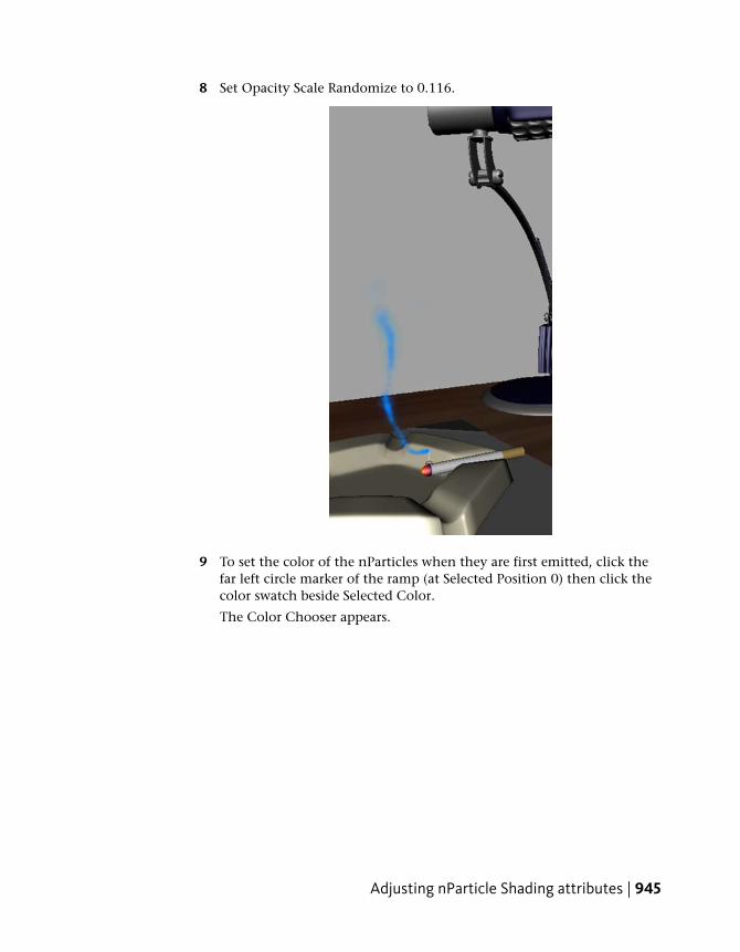
8 Set Opacity Scale Randomize to 0.116.
9 To set the color of the nParticles when they are first emitted, click thefar left circle marker of the ramp (at Selected Position 0) then click thecolor swatch beside Selected Color.
The Color Chooser appears.
Adjusting nParticle Shading attributes | 945

10 In the Numeric Input section, click the HSV tab.
11 In the Color Chooser, select white and add a little grey, or type thefollowing color values into the HSV (Hue-Saturation-Value) fields:
■ H:210
■ S: 0
■ V: 0.95
12 To set the color of the nParticles as they continue to age, click inside theramp to create a marker, set the Selected Position to 0.834, then click thecolor swatch beside Selected Color.
13 In the Color Chooser, select a shade of grey that is slightly darker thanthe color you selected for the first marker, or type the following colorvalues into the HSV (Hue-Saturation-Value) fields:
■ H:210
■ S: 0
■ V: 0.85
946 | Chapter 19 nParticles
14 Select the far right marker of the ramp (at Selected Position 1.0) and setthe color to the following color values into the HSV(Hue-Saturation-Value) fields:
■ H:191.73
■ S: 0.084
■ V: 0.85
15 Set Color Input to Normalized Age.
As each nParticle ages, its color changes from the color specified by theleft marker to the one specified by the right marker.
16 To improve the way the nParticles colors blend as they age, do thefollowing:
■ Set Interpolation to Smooth for each marker.
■ Set Color Randomize to 0.5.
When you play back the simulation, the nParticles look more like cigarettesmoke.
Adding more volume to the smoke would further improve the simulation.Instead of reducing the nParticle Opacity values, you can emit moreparticles and increase the nParticle Radius to create more smoke volume.
Adjusting nParticle Shading attributes | 947

To add volume to the nParticle smoke
1 In the Outliner, select nParticle_Smoke.
2 In the Attribute Editor, click the nParticle_SmokeShape tab.
3 In the Lifespan section, set Lifespan to 10.
4 In the Particle Size section, set Radius to 6.5.
5 In the Attribute Editor, click the Emitter_Smoke1 tab.
6 In the Basic Emitter Attributes section, set Rate (Particles/Sec) to 128.4.
7 Play back the simulation.
You can continue adjusting the Opacity Scale and Color ramps to createthe exact dissipation effect and color you want for the smoke.
948 | Chapter 19 nParticles

Open the third scene for the lessonTo ensure this lesson works as described, open the scene file namedSmoke_Simulation_3.mb. This file is in the GettingStarted directory that youset as your Maya project:
GettingStarted/nParticles/Smoke_Simulation_3.mb
Fine tuning your smoke effectWith nParticles, you can use dynamic wind generated by the Maya Nucleussolver to affect the motion of your particles. Gravity and Wind forces generatedby the Nucleus system are different from the Maya dynamic forces that youcreate with Maya Fields. Nucleus forces are internal, meaning that they onlyaffect Nucleus objects. Nucleus object that are assigned to the same Nucleussolver are affected by the same intensity of the solver’s wind and gravity.
In this section of this lesson, you create an Axial Magnitude ramp to controlthe field’s magnitude at various points in the field volume. You specify thatthe field’s magnitude gradually increases from the bottom of the volume toits top, so that as the nParticles travel through the field volume, the field’sinfluence on the nParticles increases. To finish the smoke simulation, you usethe Nucleus Wind to make the smoke drift as it rises.
NOTE If you had other Nucleus objects (nCloth objects or other nParticle objects)assigned to the same Nucleus solver, they would also be affected by the force ofthe wind.
To create an Axial Magnitude ramp
1 In the Outliner, select Field_Smoke1.
2 In the Attribute Editor, expand the Volume Control Attributes section,and browse to the Axial Magnitude section.
3 Click in the Axial Magnitude ramp to create two new markers, and createa ramp by setting the following:
InterpolationSelectedValue
Selected PositionMarker
Linear0.5200.0551
Linear0.9000.3152
Open the third scene for the lesson | 949
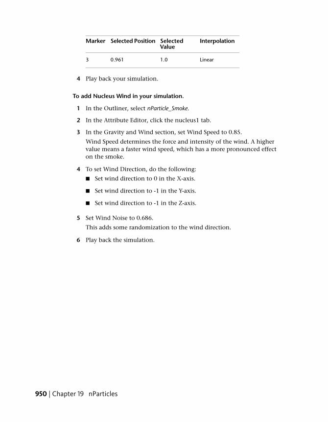
InterpolationSelectedValue
Selected PositionMarker
Linear1.00.9613
4 Play back your simulation.
To add Nucleus Wind in your simulation.
1 In the Outliner, select nParticle_Smoke.
2 In the Attribute Editor, click the nucleus1 tab.
3 In the Gravity and Wind section, set Wind Speed to 0.85.
Wind Speed determines the force and intensity of the wind. A highervalue means a faster wind speed, which has a more pronounced effecton the smoke.
4 To set Wind Direction, do the following:
■ Set wind direction to 0 in the X-axis.
■ Set wind direction to -1 in the Y-axis.
■ Set wind direction to -1 in the Z-axis.
5 Set Wind Noise to 0.686.
This adds some randomization to the wind direction.
6 Play back the simulation.
950 | Chapter 19 nParticles

To make the smoke simulation more realistic, you can set up your effectso that the cigarette smoke is rising in the first frame of the simulation.You do this by setting the nParticle object’s initial state.
To set the nParticle Object’s initial state
1 Play the simulation and stop the playback at or around frame 300.
2 In the Outliner, select nParticle_Smoke.
3 Select nSolver > Initial State > Set From Current.
4 Rewind the simulation to the start frame and play it back.
Fine tuning your smoke effect | 951
Beyond the lessonIn this lesson you created an nParticle system and used Maya Fields to influencethe behavior of the particles to create a smoke simulation effect. In addition,you learned how to:
■ Use a volume emitter with an nParticle system.
■ Use a Volume Axis field to create a disturbance in the path of yournParticles.You can also add other Maya fields, such as Turbulence, Radial, or Vortexfields to affect the behavior of nParticles.
■ Adjust nParticle lifespan so that nParticles die off at the appropriatemoment of your simulation.
■ Use the Radius Scale ramp to map per-particle radius to nParticle age.
■ Use the Opacity and Color attributes to define the color and thickness ofthe smoke.You can further optimize the color and thickness of the smoke bycontinuing to adjust the Opacity Scale and Color ramps.
■ Create an Axial Magnitude ramp to control how a field’s Magnitude affectsnParticles as they travel through the field's volume.You can fine tune your smoke simulation by adjusting the markers on thecurve to produce the desired effect of turbulence as the smoke rises.
■ Add Nucleus Wind to your nParticle effect. You can experiment with theNucleus solver’s Wind Speed, Wind Density, and Wind Direction attributesto change the direction of the rising smoke.
For more information and related techniques about nParticles and Maya Fields,refer to the Maya Help.
952 | Chapter 19 nParticles

Lesson 3: Creating a liquid simulation withnParticles
Introduction
A common use of particle systems is to simulate liquids such as flowing lava,water sprays, and mud splatters. Using nParticle Liquid Simulation attributes,you can add properties to an nParticle object so that it behaves like a liquid.For example, you can add viscosity and incompressibility properties so thatthe nParticles fill a volume uniformly and flow like a continuous substance.
When creating a liquid simulation, it is easiest to start with a small nParticlesystem (small particle count) and set the attributes that control the behaviorof the particle flow. You can then increase the density of the particle systemand edit the attributes that give the nParticles the appearance of a liquid.
In this lesson you create a small-scale liquid simulation that involves pouringWater type nParticles from a pitcher into a glass. You can then use thetechniques described in this tutorial to create larger liquid simulations.
In this lesson you learn how to:
■ Use Fill Object to create a Water style nParticle system.
Lesson 3: Creating a liquid simulation with nParticles | 953
■ Adjust nParticle Liquid Simulation attributes to create particles that lookand behave like water.
■ Cache your nParticle simulation.
■ Convert a liquid simulation to an nParticle output mesh.
■ Assign mia_material_x mental ray shaders to your nParticle output mesh.
■ Render a single frame of your nParticle simulation using mental ray forMaya renderer.
Lesson setupTo ensure this lesson works as described, open the scene file namedLiquid_Simulation_1.mb. This file is in the GettingStarted directory thatyou set as your Maya project:
GettingStarted/nParticles/Liquid_Simulation_1.mb
This scene includes textured polygon models including a desk, water pitcher,and water glass. The water pitcher mesh is animated to lift off the desk, tip topour water into the glass, then set back down on the desktop.
Creating a Water style nParticle objectIn the first step of creating your liquid simulation, you fill a polygon waterpitcher with Water style nParticles. To do this, you use the Fill Object option.
To create a Water style nParticle object
1 Select nParticles > Create nParticles > Water.
Selecting a Water style nParticle object presets some nParticleShapeattributes including turning on Liquid Simulation attributes, turning offnParticle Self Collisions, and setting the Particle Render Type to BlobbySurface.
2 In the Outliner, select geo_pitcher, which is contained in the grp_Pitcherobject.
This is the geometry that you will fill with Water style nParticles.
3 Select nParticles > Create nParticles > Fill Object > .
The Particle Fill Options window appears.
954 | Chapter 19 nParticles
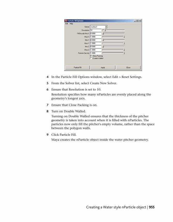
4 In the Particle Fill Options window, select Edit > Reset Settings.
5 From the Solver list, select Create New Solver.
6 Ensure that Resolution is set to 10.
Resolution specifies how many nParticles are evenly placed along thegeometry’s longest axis.
7 Ensure that Close Packing is on.
8 Turn on Double Walled.
Turning on Double Walled ensures that the thickness of the pitchergeometry is taken into account when it is filled with nParticles. Theparticles now only fill the pitcher's empty volume, rather than the spacebetween the polygon walls.
9 Click Particle Fill.
Maya creates the nParticle object inside the water pitcher geometry.
Creating a Water style nParticle object | 955
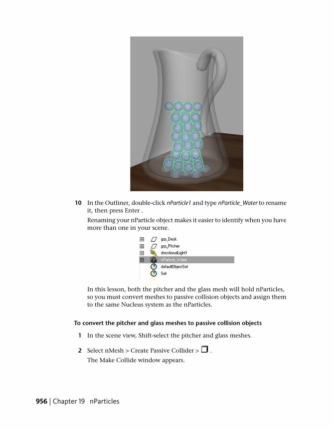
10 In the Outliner, double-click nParticle1 and type nParticle_Water to renameit, then press Enter .
Renaming your nParticle object makes it easier to identify when you havemore than one in your scene.
In this lesson, both the pitcher and the glass mesh will hold nParticles,so you must convert meshes to passive collision objects and assign themto the same Nucleus system as the nParticles.
To convert the pitcher and glass meshes to passive collision objects
1 In the scene view, Shift-select the pitcher and glass meshes.
2 Select nMesh > Create Passive Collider > .
The Make Collide window appears.
956 | Chapter 19 nParticles

3 From the Solver list, select nucleus1.
4 Click Make Collide.
5 Rename the pitcher and glass nRigid objects in the Outliner. For example,rename nRigid1 and nRigid2as nRigid_Pitcher and nRigid_Glass respectively.
6 Play back the simulation.
When you play back the simulation, notice that the nParticles do notbehave as you might expect. Rather than immediately falling to thebottom of the pitcher like water, they fall slowly, as if the simulation isplaying in slow motion. To make the nParticles behave realistically, youcan set the Nucleus Space Scale for the simulation.
For more information about Space Scale, see Setting Nucleus Space Scaleon page 922.
To set Space Scale
1 In the Attribute Editor, click the nucleus1 tab.
2 In the Scale Attributes section, set the Space Scale to 0.01.
When you reduce the Space Scale value, Maya evaluates the nParticlesystem as if the particles are much smaller in size. This results in a visiblyincreased gravitational effect on the nParticles.
3 Rewind the simulation to the start frame, then play it back.
Creating a Water style nParticle object | 957

When you play back the simulation, notice that the nParticles are stillcontained in the pitcher, but they occupy a small amount of the pitcher’svolume. Also, the nParticles appear to be pushing down as if they areunder a force of pressure or compression. In the next section, you beginadjusting the Liquid Simulation attributes that make the nParticles lookand behave more like a liquid.
Adjusting Liquid Simulation attributesOne of the main characteristics of water is its volume uniformly fills the areainside a holding vessel or container. To give nParticles this volumecharacteristic, there needs to be space between individual particles. Be awarethat having too much space can hinder the fluidity of the particles, which isanother important characteristic of a liquid simulation.
Using the Liquid Radius Scale attribute, you can control the amount of spacebetween nParticles.
958 | Chapter 19 nParticles

Adjusting the liquid volume
To set Liquid Radius Scale and create liquid volume
1 In the Outliner, select nParticle_Water.
2 In the Attribute Editor, click the nParticle_WaterShape tab.
3 In the Liquid Simulation section, ensure that Enable Liquid Simulationis on.
4 Set Liquid Radius Scale to 2.0.
5 Play back the simulation.
The nParticles are now stacked on top of each other, creating more volumein the pitcher.
For this liquid simulation, you want the nParticles to fill one-third of thepitcher. You can add more volume to the nParticles by adjusting theNucleus solver Substeps and Max Collision Iterations.
6 Set Substeps and Max Collision Iterations by doing the following:
■ In the Attribute Editor, click the nucleus1 tab.
Adjusting Liquid Simulation attributes | 959

■ In the Solver Attributes section, set Substeps to 7.
■ Set Max Collision Iterations to 10.
7 Play back the simulation.
The nParticles now fill the water pitcher, and when the pitcher tilts topour, the nParticles have enough volume to exit and fill the glass.
More about Liquid Radius Scale
Be aware that Liquid Radius Scale can be affected by other nParticle attributessuch as Radius and Collide Width Scale. For example, Liquid Radius Scale usesthe nParticle object's Radius to determine how nParticles overlap, and anychange in the nParticle Radius affects how nParticles overlap in the liquidsimulation.
Adjusting the Nucleus solver Substeps and Max Collision Iterations also affectsthe volume that is generated by the Liquid Radius Scale value. You canexperiment with these settings by changing Substeps to 10 and Max CollisionIterations to 15 and observing how your liquid simulation is affected.
In the next section of this lesson, you adjust nParticle Collide Scale Widthand Incompressibility attributes to add fluidity to your simulation.
Adding fluidity to the nParticlesTo make it easier to see how the nParticles interact with the pitcher and glassobjects, you can turn on the Solver Display to see the nParticle collisionvolume. Collision volumes are a non-renderable surface offset from eachnParticle radius that the nucleus solver uses when calculating collisionsbetween Nucleus objects.
To edit Collide Width Scale and add fluidity
1 In the Outliner, select nParticle_Water.
2 In the Attribute Editor, click the nParticle_WaterShape tab.
960 | Chapter 19 nParticles

3 In the Collisions section, select Collision Thickness from the SolverDisplay list.
4 Set Collide Width Scale to 0.6.
For liquid simulations, set Collide Width Scale to a value that is one-thirdthe nParticle object Radius value.
5 Play the simulation, and stop at frame 40.
6 In the scene view, dolly and tumble so that you get a close-up view ofthe nParticles at the bottom of the pitcher.
The nParticles occupy the pitcher in two distinct layers one on top of theother. In the bottom layer, the nParticles are evenly spaced and level,while in the upper layer, there are gaps between particles. Since the toplayer of nParticles represent the surface of the liquid, the gaps betweenparticles create a surface that is uneven and unlike the surface of water.
Increasing Incompressibility decreases the tendency of the particles to bepushed together. This forces the nParticles into a more uniform distributionthroughout the volume, which creates a smoother surface for the liquid.
Adding fluidity to the nParticles | 961
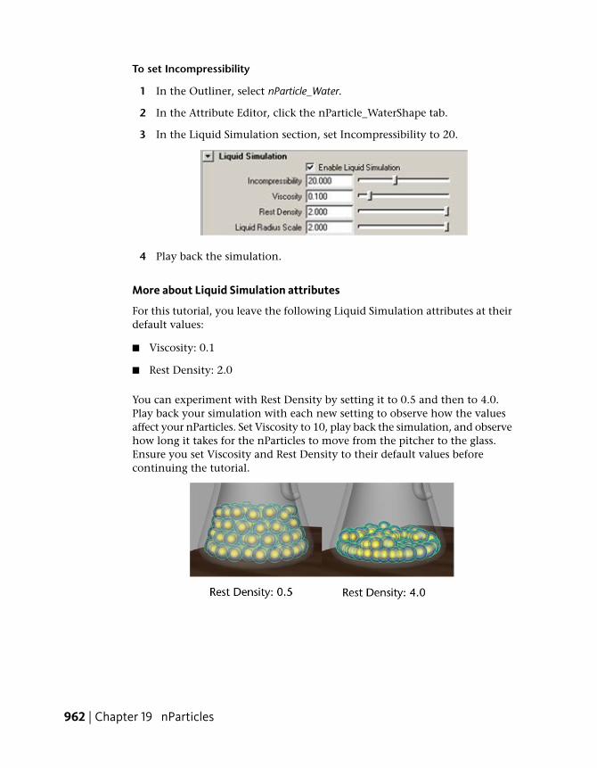
To set Incompressibility
1 In the Outliner, select nParticle_Water.
2 In the Attribute Editor, click the nParticle_WaterShape tab.
3 In the Liquid Simulation section, set Incompressibility to 20.
4 Play back the simulation.
More about Liquid Simulation attributes
For this tutorial, you leave the following Liquid Simulation attributes at theirdefault values:
■ Viscosity: 0.1
■ Rest Density: 2.0
You can experiment with Rest Density by setting it to 0.5 and then to 4.0.Play back your simulation with each new setting to observe how the valuesaffect your nParticles. Set Viscosity to 10, play back the simulation, and observehow long it takes for the nParticles to move from the pitcher to the glass.Ensure you set Viscosity and Rest Density to their default values beforecontinuing the tutorial.
962 | Chapter 19 nParticles
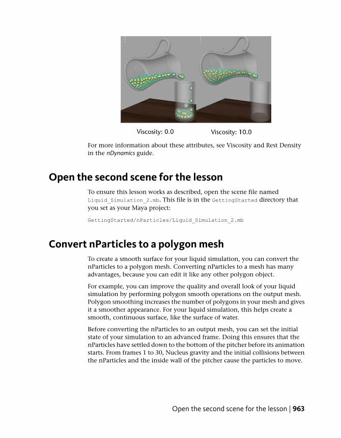
For more information about these attributes, see Viscosity and Rest Densityin the nDynamics guide.
Open the second scene for the lessonTo ensure this lesson works as described, open the scene file namedLiquid_Simulation_2.mb. This file is in the GettingStarted directory thatyou set as your Maya project:
GettingStarted/nParticles/Liquid_Simulation_2.mb
Convert nParticles to a polygon meshTo create a smooth surface for your liquid simulation, you can convert thenParticles to a polygon mesh. Converting nParticles to a mesh has manyadvantages, because you can edit it like any other polygon object.
For example, you can improve the quality and overall look of your liquidsimulation by performing polygon smooth operations on the output mesh.Polygon smoothing increases the number of polygons in your mesh and givesit a smoother appearance. For your liquid simulation, this helps create asmooth, continuous surface, like the surface of water.
Before converting the nParticles to an output mesh, you can set the initialstate of your simulation to an advanced frame. Doing this ensures that thenParticles have settled down to the bottom of the pitcher before its animationstarts. From frames 1 to 30, Nucleus gravity and the initial collisions betweenthe nParticles and the inside wall of the pitcher cause the particles to move.
Open the second scene for the lesson | 963

For a realistic effect, you want the water to be motionless at the bottom of thepitcher at the start of the simulation.
To set the initial state of the nParticles
1 Play the simulation and stop the playback at or around frame 30.
2 In the Outliner, select nParticle_Water.
3 Select nSolver > Initial State > Set From Current.
4 Rewind the simulation to the start frame.
To convert your nParticle object to a polygon mesh
1 In the Outliner, select nParticle_Water.
2 Select Modify > Convert > nParticle to Polygons.
The PolySurface1 object appears in the Outliner, and a newpolySurfaceShape node appears in the Attribute Editor.
3 Rename the new PolySurface1 polygon object to Water_Mesh in theOutliner.
4 In the Attribute Editor, select the nParticle_WaterShape tab.
964 | Chapter 19 nParticles
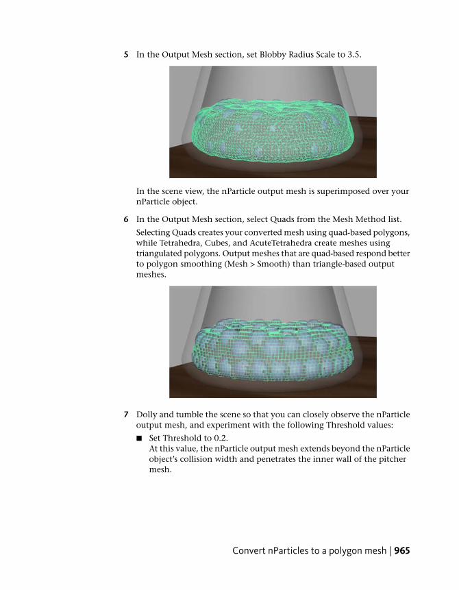
5 In the Output Mesh section, set Blobby Radius Scale to 3.5.
In the scene view, the nParticle output mesh is superimposed over yournParticle object.
6 In the Output Mesh section, select Quads from the Mesh Method list.
Selecting Quads creates your converted mesh using quad-based polygons,while Tetrahedra, Cubes, and AcuteTetrahedra create meshes usingtriangulated polygons. Output meshes that are quad-based respond betterto polygon smoothing (Mesh > Smooth) than triangle-based outputmeshes.
7 Dolly and tumble the scene so that you can closely observe the nParticleoutput mesh, and experiment with the following Threshold values:
■ Set Threshold to 0.2.At this value, the nParticle output mesh extends beyond the nParticleobject’s collision width and penetrates the inner wall of the pitchermesh.
Convert nParticles to a polygon mesh | 965

■ Set Threshold to 1.5.At this value, the nParticle output mesh cuts into the nParticle object,and no longer surrounds the nParticles.
■ Set Threshold 0.6.
8 Set Mesh Triangle Size to 0.2.
966 | Chapter 19 nParticles
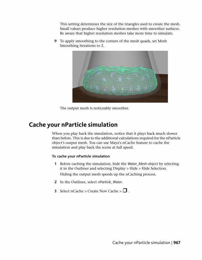
This setting determines the size of the triangles used to create the mesh.Small values produce higher resolution meshes with smoother surfaces.Be aware that higher resolution meshes take more time to simulate.
9 To apply smoothing to the corners of the mesh quads, set MeshSmoothing Iterations to 2.
The output mesh is noticeably smoother.
Cache your nParticle simulationWhen you play back the simulation, notice that it plays back much slowerthan before. This is due to the additional calculations required for the nParticleobject’s output mesh. You can use Maya's nCache feature to cache thesimulation and play back the scene at full speed.
To cache your nParticle simulation
1 Before caching the simulation, hide the Water_Mesh object by selectingit in the Outliner and selecting Display > Hide > Hide Selection.
Hiding the output mesh speeds up the nCaching process.
2 In the Outliner, select nParticle_Water.
3 Select nCache > Create New Cache > .
Cache your nParticle simulation | 967

The Create nCache Options window appears.
4 In the Create nCache Options window, do the following:
■ Set the Cache directory to the folder where you want your cachessaved.
■ Set the Cache name to LiquidSimulationCache.
■ For File distribution, select One file.
■ Click Create.
Maya plays the scene automatically and stores the frames in the directoryyou specified.
5 When it is finished, play back the simulation.
Notice that the scene now plays back faster. You can also scrub slowlythrough the timeline and view your simulation frame-by-frame. If youchange any of the nParticle attribute settings, create a new cache to seeyour changes.
In the next section of this lesson, you use the nParticle cache to help optimizespecific areas of the simulation.
Adding Motion StreakYou can set the Motion Streak attribute to optimize the motion of the nParticlesduring the pouring sequence of the animation. Motion Streak is useful forcreating a motion blur type of effect, and for shaping the flow of liquids.
968 | Chapter 19 nParticles
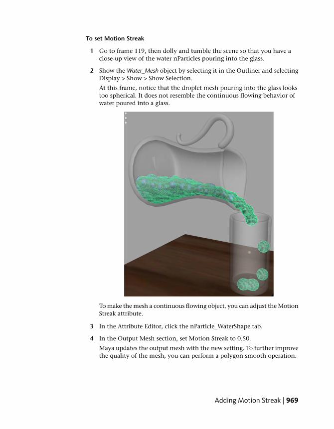
To set Motion Streak
1 Go to frame 119, then dolly and tumble the scene so that you have aclose-up view of the water nParticles pouring into the glass.
2 Show the Water_Mesh object by selecting it in the Outliner and selectingDisplay > Show > Show Selection.
At this frame, notice that the droplet mesh pouring into the glass lookstoo spherical. It does not resemble the continuous flowing behavior ofwater poured into a glass.
To make the mesh a continuous flowing object, you can adjust the MotionStreak attribute.
3 In the Attribute Editor, click the nParticle_WaterShape tab.
4 In the Output Mesh section, set Motion Streak to 0.50.
Maya updates the output mesh with the new setting. To further improvethe quality of the mesh, you can perform a polygon smooth operation.
Adding Motion Streak | 969

5 Select the mesh then, from the Polygons menu set, select Mesh > Smooth.
The mesh is noticeably smoother and looks more like a liquid. In thenext section, you will assign material shaders to the pitcher, glass, andwater meshes. You will then render single frames of the simulation usingmental ray for Maya.
Open the third scene for the lessonTo ensure this lesson works as described, open the scene file namedLiquid_Simulation_3.mb. This file is in the GettingStarted directory thatyou set as your Maya project:
GettingStarted/nParticles/Liquid_Simulation_3.mb
970 | Chapter 19 nParticles

Render your liquid simulationIn this section, you render your nParticle effect using the mental ray for Mayarenderer. Since rendering a particle effect can take several minutes to an hour,in this lesson, you only render selected frames of the simulation. Renderingsimulated frames is the easiest way to see how some attributes affect yoursimulation.
To prepare your scene for rendering, you assign mental ray mia_material_xshaders to the pitcher, glass, and water meshes. Lights have been created andplaced in the scene so that realistic shadows and reflections appear in therendered frame. The scene also includes a camera named renderCam that ispositioned for the rendered view. For more information about rendering, seethe Rendering and Render Setup guide.
Preparing to render
To prepare your scene and workspace for rendering, you will do the following:
■ Cache your simulation so that you can play it or scrub through it to locatethe simulated frame you want to render.
■ Change the view arrangement of your Maya workspace to make it easierto assign material shaders to meshes and view rendered frames of yoursimulation.
■ Show hidden light objects and the camera you use to render a simulatedframe.
To cache your simulation
1 In the Outliner, select nParticle_Water.
2 Select nCache > Create New Cache > .
The Create nCache Options window appears.
3 In the Create nCache Options window, do the following:
■ Set the Cache directory to the folder where you want your cachessaved.
■ Set the Cache name to LiquidSimulationCache.
■ For File distribution, select One File.
■ Click Create.
Render your liquid simulation | 971

4 Go to the beginning of the playback range.
To change the view arrangement and display hidden objects
1 Select Windows > Saved Layouts > Hypershade/Render/Persp.
The Hypergraph, Render View, and the current perspective view aredisplayed. This view arrangement makes it easier to assign shaders toyour objects and to view rendered frames of your simulation.
2 Open the Outliner in a separate window by selecting Window > Outliner.
3 Hide the nParticle_ Water object by selecting it in Outliner, then selectingDisplay > Hide > Hide Selection.
4 Show the Water_Mesh object by selecting it in the Outliner then selectingDisplay > Show > Show Selection.
5 In the Outliner, Ctrl-click the main, rim, and fill lights, then select Display> Show >Show Selection.
The lights used for rendering the simulation appear in the scene.
6 In the perspective view, select Panels > Perspective > renderCam.
You now view the scene through the camera that you will use to render.
Assigning material shadersTo prepare the geometry for rendering, you assign the mental raymia_material_x shader to the pitcher, glass, and water meshes. Using themia_material_x shader presets for the glass and water provides a quick andeasy way to have proper refraction, reflectivity, and transparency values seton these materials. For more information about material shaders, see themental ray mia_material/mia_material_x shader attributes section in theRending and Render Setup guide.
To assign a material to the pitcher and glass objects
1 In the Hypershade, on the Create tab, click Create Maya Nodes and selectCreate mental ray Nodes from the drop-down list.
The Hypershade now shows the list of mental ray shader nodes.
2 Click Materials to open the list of mental ray material shaders.
3 Select mia_material_x from the Materials list.
972 | Chapter 19 nParticles

A mia_material_x material swatch appears in the Work Area tab of theHypershade, and the material attributes appear in the Attribute Editor.
4 In the Attribute Editor, rename the material to mia_material_pitcher.
5 Click and hold the Presets button, select GlassThin, then Replace(GlassThin > Replace).
6 In the Refraction section, click the color swatch beside Color.
The Color Chooser appears.
7 In the Color Chooser, type the following color values into the RGB fields:
■ R: 0.190
■ G: 0.574
■ B: 0.190
8 Click Accept.
9 In the Outliner, select the grp_Pitcher object.
10 To assign the material to the pitcher, in the Work Area tab of theHypershade, right-click mia_material_glass then select Assign Material ToSelection from the marking menu.
In the scene view, the pitcher turns black. You can only see the true colorand texture of the material after the frame is rendered using mental rayfor Maya.
Assigning material shaders | 973
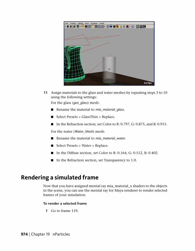
11 Assign materials to the glass and water meshes by repeating steps 3 to 10using the following settings:
For the glass (geo_glass) mesh:
■ Rename the material to mia_material_glass.
■ Select Presets > GlassThin > Replace.
■ In the Refraction section, set Color to R: 0.797, G: 0.875, and B: 0.915.
For the water (Water_Mesh) mesh:
■ Rename the material to mia_material_water.
■ Select Presets > Water > Replace.
■ In the Diffuse section, set Color to R: 0.164, G: 0.512, B: 0.402.
■ In the Refraction section, set Transparency to 1.0.
Rendering a simulated frameNow that you have assigned mental ray mia_material_x shaders to the objectsin the scene, you can use the mental ray for Maya renderer to render selectedframes of your simulation.
To render a selected frame
1 Go to frame 119.
974 | Chapter 19 nParticles

You will render this frame where the water nParticles pour into the glass.
2 In the Render View, select Options > Render Settings
.
The Render Settings window appears.
3 From the Render Using list, select mental ray.
4 Click the Common tab and set the following:
■ In the Renderable Cameras section, select renderCam from theRenderable Camera list.
■ In the Image Size section, select 320×240 from the Presets list.
5 Click the Quality tab, and do the following:
■ From the Quality Presets list, select Production.
■ In the Raytracing section, turn on Raytracing.
■ Set Shadows to 4.
6 Click the Indirect Lighting tab, and in the Caustics section, turn onCaustics.
7 Click Close to close the Render Settings window.
8 To render the current frame, in the Render View, select Render > Render> Current (renderCam).
The current frame appears as a rendered image in the Render View.
Rendering a simulated frame | 975

You can continue to make changes to the render settings, change therenderCam view, or select another simulated frame to render. After youare satisfied with your render settings, you can render the frame as afull-size image.
To render a full-size image
1 In the Render View, select Options > Render Settings.
2 Click the Common tab and in the Image Size section, select 640×480from the Presets list.
3 From the Rendering menu set, select Render > Render Current Frame.
Beyond the lessonIn this lesson you learned how to:
■ Use Fill Object to create an nParticle system.
■ Create passive collision objects to contain your nParticles.
■ Adjust the Nucleus solver’s Space Scale attribute to suit the scale of yoursimulation.
976 | Chapter 19 nParticles

■ Adjust Liquid Simulation attributes to set the volume and fluiditycharacteristics of your liquid nParticles.You can continue to adjust the Liquid Simulation attributes, such as LiquidRadius Scale and Viscosity, to create liquid simulations of thicker substancessuch as oil, mud, or lava.
■ Create and play back nParticle caches.
■ Convert your nParticle object to a polygon mesh.
■ Optimize the appearance of your nParticle output mesh using Output Meshattributes such as Threshold, Mesh Smooth Iterations, and Motion Streak.
■ Assign mia_material_x mental ray shaders to your nParticle output mesh.
■ Render a single frame of your nParticle simulation using the mental rayfor Maya renderer.
Beyond the lesson | 977

978
Live
IntroductionMaya® LiveTM simplifies the process of matchmoving. Matchmoving is a processwhere you match the camera or object movement in a live-action shot with thecamera in Maya. This subsequently lets you place your 3D objects into live-actionfootage.
Matchmoving is an iterative process where the camera movement for the Mayacamera is calculated using processes of tracking and solving.
Objects are tracked in the live action scene and a solver then calculates thecamera position for a given image. This chapter includes the following lessons:
■ Lesson 1 Track and solve: Introduction on page 983
■ Lesson 2 Solving with survey data: Introduction on page 1002
About LiveImagine that you must replace the contents of a live-action shot of a fence witha fence modeled in Maya. In the live-action shot, the camera sweeps aroundthe fence. You can use Live to animate a Maya camera that sweeps around yourmodeled fence in the same way. When you render the Maya fence from thiscamera, it will have the same camera perspective as the live-action fence. Youcan therefore composite them together precisely.
20
979

Live can also match the movement of objects in the live-action shot. Supposeyou want to replace the hat of a moving, live-action person with a cartoonhat created in Maya. You can use Live to create 3D locators that follow themovement of certain points on the live-action hat. You then attach a hatcreated in Maya to these moving points, so that the rendered Maya hat followsthe movements of the live-action person. The steps for matching objectmovement are about the same as matching the camera.
To use Live, you do the following major tasks in order:
Setting up
You begin by loading digital images of the live-action shot. In this lesson,you’ll use images scanned from film footage.
Images appear on an image plane. This plane is part of the Maya camera. Itdisplays images as part of a background.
980 | Chapter 20 Live
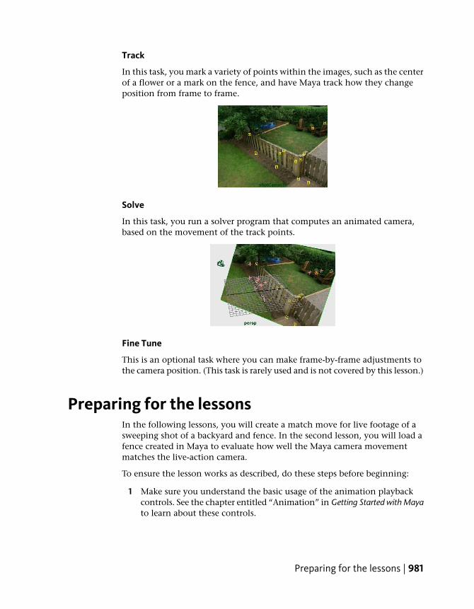
Track
In this task, you mark a variety of points within the images, such as the centerof a flower or a mark on the fence, and have Maya track how they changeposition from frame to frame.
Solve
In this task, you run a solver program that computes an animated camera,based on the movement of the track points.
Fine Tune
This is an optional task where you can make frame-by-frame adjustments tothe camera position. (This task is rarely used and is not covered by this lesson.)
Preparing for the lessonsIn the following lessons, you will create a match move for live footage of asweeping shot of a backyard and fence. In the second lesson, you will load afence created in Maya to evaluate how well the Maya camera movementmatches the live-action camera.
To ensure the lesson works as described, do these steps before beginning:
1 Make sure you understand the basic usage of the animation playbackcontrols. See the chapter entitled “Animation” in Getting Started with Mayato learn about these controls.
Preparing for the lessons | 981
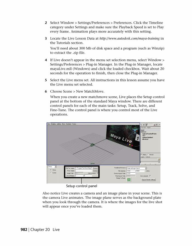
2 Select Window > Settings/Preferences > Preferences. Click the Timelinecategory under Settings and make sure the Playback Speed is set to Playevery frame. Animation plays more accurately with this setting.
3 Locate the Live Lesson Data at http://www.autodesk.com/maya-training inthe Tutorials section.
You’ll need about 300 Mb of disk space and a program (such as Winzip)to extract the .zip file.
4 If Live doesn’t appear in the menu set selection menu, select Window >Settings/Preferences > Plug-in Manager. In the Plug-in Manager, locatemayaLive.mll (Windows) and click the loaded checkbox. Wait about 20seconds for the operation to finish, then close the Plug-in Manager.
5 Select the Live menu set. All instructions in this lesson assume you havethe Live menu set selected.
6 Choose Scene > New MatchMove.
When you create a new matchmove scene, Live places the Setup controlpanel at the bottom of the standard Maya window. There are differentcontrol panels for each of the main tasks: Setup, Track, Solve, andFine-Tune. The control panel is where you control most of the Liveoperations.
Also notice Live creates a camera and an image plane in your scene. This isthe camera Live animates. The image plane serves as the background platewhen you look through the camera. It is where the images for the live shotwill appear once you’ve loaded them.
982 | Chapter 20 Live

Lesson setupYou begin the lesson by loading digital images of a live-action sequence. You’llwork with images we created for your use.
To load and set up the images for the lesson
1 If you haven’t already done so, download and extract the Maya LiveLesson Data at http://www.autodesk.com/maya-training in the Tutorialssection.
2 In the Setup control panel, click the Browse button next to the Full ResImage box.
3 Navigate to the MayaLiveLessonData/sourceimages directory that youextracted and select any image file from the list, such asshot1BG.rgb.0001.
4 Click the Open button. Live loads the entire image sequence, fromshot1BG.rgb.0001 to shot1BG.rgb.0240.
5 From the Predefined Filmbacks list (on the Setup control panel), choose35mm Full Aperture.
Filmback is the aspect ratio (width/height) of the exposed film negativeused during filming. Before using Live, you need to find out whichfilmback was used during filming. Without it, Live cannot determine thecorrect angle of view (camera aperture) and focal length.
NOTE If the images do not appear on the image plane, you may need toadjust the image cache settings. Click the Cache option on the far left todisplay the cache settings. Set Texture Method to Image. If the images stilldo not appear, try selecting None.
Lesson 1: Track and solve
IntroductionThis lesson guides you through the main tasks in Live: tracking and solving.In this lesson you learn how to:
■ Review footage to determine the location of tracking points.
Lesson setup | 983

■ Position tracking points for the live-action footage.
■ Track points in the scene
■ Evaluate how closely points are tracked using the Track Summary panel.
■ Modify the location of tracking points for a scene.
■ Import track points into Maya.
■ Solve for the camera movement.
■ Evaluate and modify the solution that the Solver creates.
Tracking provides Live with information about the way objects in the shotappear to move. Just as objects move in your field of view when you walk bythem, the way objects move in the camera view gives Live information onhow the camera moved during filming.
You’ll track points for various spots, such as a mark on the fence. To track apoint, you mark each spot in the image and have Live run a tracker thatautomatically follows the point’s movement from frame to frame. The resultis called a track point.
Later, in the solve task, Live will animate a Maya camera based on the trackpoint movement.
Tracking preparationWhich spots should you track? To answer this question, do these steps:
To review a shot and plan for the tracking
1 Open the Track control panel by clicking the menu on the far left of thecontrol panel and choosing Track.
Above the Track control panel, Live displays preset view panels. The viewpanels match the needs of tracking. The following illustration labels thesepanels, shown the way they might look at the end of the lesson.
984 | Chapter 20 Live
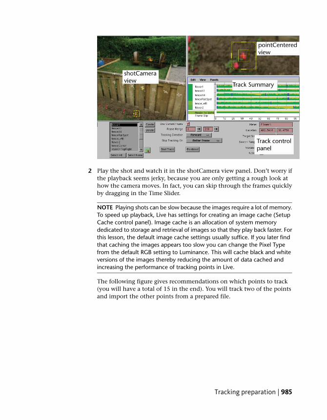
2 Play the shot and watch it in the shotCamera view panel. Don’t worry ifthe playback seems jerky, because you are only getting a rough look athow the camera moves. In fact, you can skip through the frames quicklyby dragging in the Time Slider.
NOTE Playing shots can be slow because the images require a lot of memory.To speed up playback, Live has settings for creating an image cache (SetupCache control panel). Image cache is an allocation of system memorydedicated to storage and retrieval of images so that they play back faster. Forthis lesson, the default image cache settings usually suffice. If you later findthat caching the images appears too slow you can change the Pixel Typefrom the default RGB setting to Luminance. This will cache black and whiteversions of the images thereby reducing the amount of data cached andincreasing the performance of tracking points in Live.
The following figure gives recommendations on which points to track(you will have a total of 15 in the end). You will track two of the pointsand import the other points from a prepared file.
Tracking preparation | 985
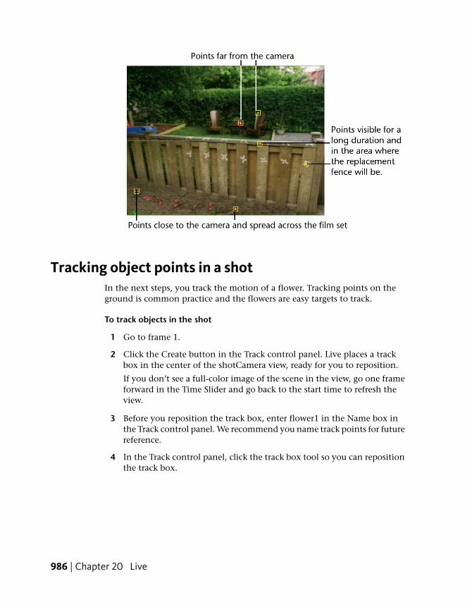
Tracking object points in a shotIn the next steps, you track the motion of a flower. Tracking points on theground is common practice and the flowers are easy targets to track.
To track objects in the shot
1 Go to frame 1.
2 Click the Create button in the Track control panel. Live places a trackbox in the center of the shotCamera view, ready for you to reposition.
If you don’t see a full-color image of the scene in the view, go one frameforward in the Time Slider and go back to the start time to refresh theview.
3 Before you reposition the track box, enter flower1 in the Name box inthe Track control panel. We recommend you name track points for futurereference.
4 In the Track control panel, click the track box tool so you can repositionthe track box.
986 | Chapter 20 Live
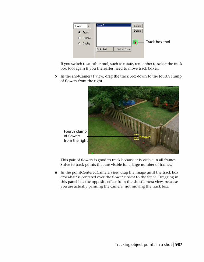
If you switch to another tool, such as rotate, remember to select the trackbox tool again if you thereafter need to move track boxes.
5 In the shotCamera1 view, drag the track box down to the fourth clumpof flowers from the right.
This pair of flowers is good to track because it is visible in all frames.Strive to track points that are visible for a large number of frames.
6 In the pointCenteredCamera view, drag the image until the track boxcross-hair is centered over the flower closest to the fence. Dragging inthis panel has the opposite effect from the shotCamera view, becauseyou are actually panning the camera, not moving the track box.
Tracking object points in a shot | 987

Notice that the track box resizes if you drag the edges. For this track point,keep the boxes at the default size. Choose Edit > Undo if you resize itaccidentally. It may require a number of Undo commands to return tothe original configuration of the track box.
The point you are tracking is at the center of the track box cross-hair. Totrack this point, Live uses the pattern of pixels defined by the inner box.The outer box is the range Live searches for the target pattern.
7 Make sure Tracking Direction is set to Forward.
During the course of creating track points, you will change this settingoften. Depending on the situation, you might track Forward, Backward,or Bidirectional.
8 Click the Start Track button.
First a progress dialog box appears, then a movie of the track point. Thesepoint-centered movies are important tools for evaluating how closely thetrack point stays on target (see the following steps).
988 | Chapter 20 Live

Evaluating the tracking of a pointMaking sure the track point stays on target will help later when you solve.Don’t worry if the connection between tracking and solving is not clear yet.For now, simply identify major tracking errors by following these steps:
To evaluate the flower1 track
1 Review the movie file that Live generates at the end of tracking.
Identify any areas where the cross-hair slips noticeably from the originalposition on the flower. This takes some judgment. Since the flowerchanges shape over time, you must visualize where the original pointwould be as the camera perspective changes.
If the cross-hair appears to stay within two pixels of the original targetpoint, you have tracked the flower successfully. If the cross-hair movescompletely off the flower or the tracking stops before it reaches the lastframe, you must track again. Delete the track point (click Delete in theTrack control panel), return to frame 1, position the track box cross hairexactly in the center of the flower closest to the fence, and click StartTrack.
2 Close the Movieplayer window.
3 Look at the graph in the Track Summary panel.
Evaluating the tracking of a point | 989
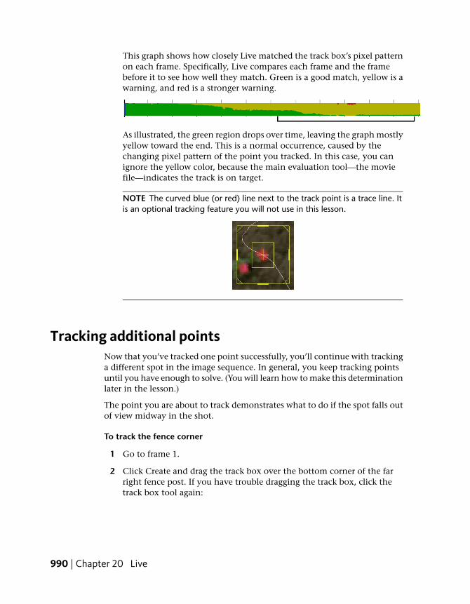
This graph shows how closely Live matched the track box’s pixel patternon each frame. Specifically, Live compares each frame and the framebefore it to see how well they match. Green is a good match, yellow is awarning, and red is a stronger warning.
As illustrated, the green region drops over time, leaving the graph mostlyyellow toward the end. This is a normal occurrence, caused by thechanging pixel pattern of the point you tracked. In this case, you canignore the yellow color, because the main evaluation tool—the moviefile—indicates the track is on target.
NOTE The curved blue (or red) line next to the track point is a trace line. Itis an optional tracking feature you will not use in this lesson.
Tracking additional pointsNow that you’ve tracked one point successfully, you’ll continue with trackinga different spot in the image sequence. In general, you keep tracking pointsuntil you have enough to solve. (You will learn how to make this determinationlater in the lesson.)
The point you are about to track demonstrates what to do if the spot falls outof view midway in the shot.
To track the fence corner
1 Go to frame 1.
2 Click Create and drag the track box over the bottom corner of the farright fence post. If you have trouble dragging the track box, click thetrack box tool again:
990 | Chapter 20 Live

3 In the PointCenteredCamera view, position the track box to match thefollowing illustration.
Knowing where to position the track box involves two important factors.One factor is the pattern framed by the inner target box. This patternmust have at least some contrast and must be distinct from thesurrounding region that is framed by the outer box. By having a distinctpattern within the inner target, you will prevent the tracker from jumpingoff target and onto a similar pattern.
Another important factor is choosing where you place the cross-hair. Youwant it to be over a spot that you can recognize in later frames when thepattern changes. By aligning the vertical cross-hair line with the postedge and the horizontal cross-hair line with the bottom of the post, youcan identify this same spot in later frames.
4 Type fenceCorner in the Name setting.
5 Click Start Track.
The tracker stops around frame 60 or 80 because the corner falls out ofview. The track box also moves off target toward the end. You will correctboth of these tracking problems in the next steps.
Tracking additional points | 991
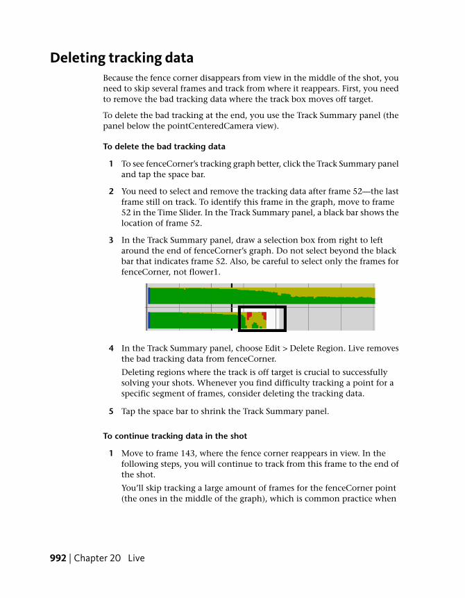
Deleting tracking dataBecause the fence corner disappears from view in the middle of the shot, youneed to skip several frames and track from where it reappears. First, you needto remove the bad tracking data where the track box moves off target.
To delete the bad tracking at the end, you use the Track Summary panel (thepanel below the pointCenteredCamera view).
To delete the bad tracking data
1 To see fenceCorner’s tracking graph better, click the Track Summary paneland tap the space bar.
2 You need to select and remove the tracking data after frame 52—the lastframe still on track. To identify this frame in the graph, move to frame52 in the Time Slider. In the Track Summary panel, a black bar shows thelocation of frame 52.
3 In the Track Summary panel, draw a selection box from right to leftaround the end of fenceCorner’s graph. Do not select beyond the blackbar that indicates frame 52. Also, be careful to select only the frames forfenceCorner, not flower1.
4 In the Track Summary panel, choose Edit > Delete Region. Live removesthe bad tracking data from fenceCorner.
Deleting regions where the track is off target is crucial to successfullysolving your shots. Whenever you find difficulty tracking a point for aspecific segment of frames, consider deleting the tracking data.
5 Tap the space bar to shrink the Track Summary panel.
To continue tracking data in the shot
1 Move to frame 143, where the fence corner reappears in view. In thefollowing steps, you will continue to track from this frame to the end ofthe shot.
You’ll skip tracking a large amount of frames for the fenceCorner point(the ones in the middle of the graph), which is common practice when
992 | Chapter 20 Live

creating track points. In general, track as many frames as possible foreach point and skip, retrack, or delete any frames where the tracker doesnot stay on target.
2 Reposition the track box over the fence corner. In thepointCenteredCamera view, align the vertical cross-hair line with theedge of the fence post and the horizontal cross-hair line with the bottomof the post.
3 Shorten the track box’s inner target box by clicking the inner target box’sbottom edge and dragging up as shown below. The tracker will not workif the target area extends beyond the image.
4 In the Track control panel, click Start Track. If the tracker successfullytracks to the last frame, you’ll see a graph similar to the following
Deleting tracking data | 993
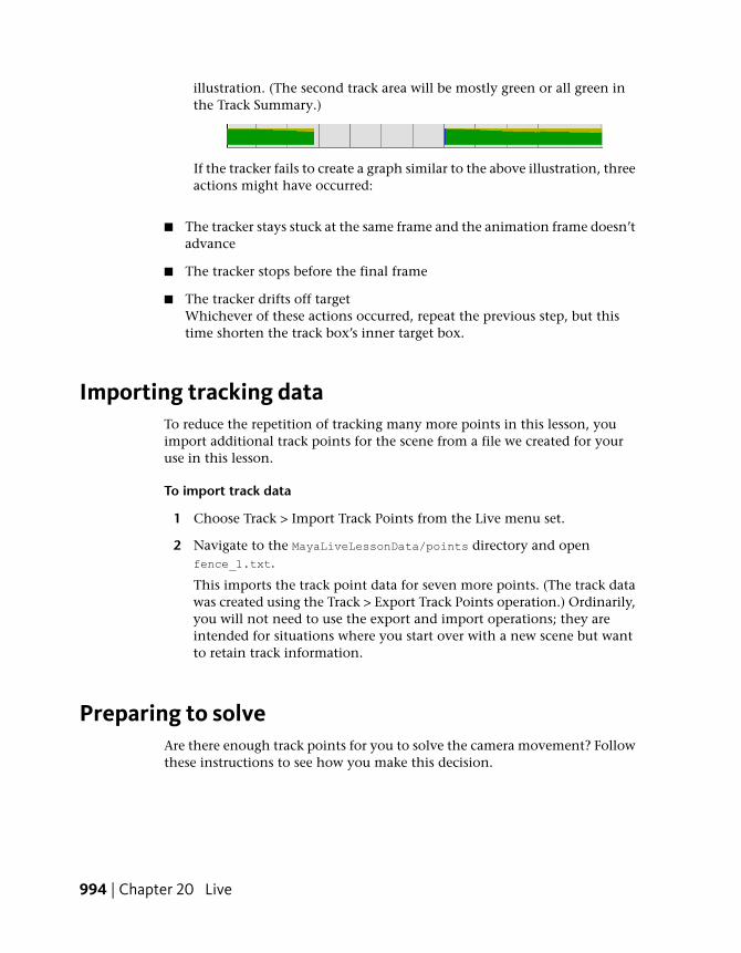
illustration. (The second track area will be mostly green or all green inthe Track Summary.)
If the tracker fails to create a graph similar to the above illustration, threeactions might have occurred:
■ The tracker stays stuck at the same frame and the animation frame doesn’tadvance
■ The tracker stops before the final frame
■ The tracker drifts off targetWhichever of these actions occurred, repeat the previous step, but thistime shorten the track box’s inner target box.
Importing tracking dataTo reduce the repetition of tracking many more points in this lesson, youimport additional track points for the scene from a file we created for youruse in this lesson.
To import track data
1 Choose Track > Import Track Points from the Live menu set.
2 Navigate to the MayaLiveLessonData/points directory and openfence_1.txt.
This imports the track point data for seven more points. (The track datawas created using the Track > Export Track Points operation.) Ordinarily,you will not need to use the export and import operations; they areintended for situations where you start over with a new scene but wantto retain track information.
Preparing to solveAre there enough track points for you to solve the camera movement? Followthese instructions to see how you make this decision.
994 | Chapter 20 Live

To decide if you are ready to solve for the camera movement
1 In the Track Summary panel, choose View > Frame All.
2 For each frame, make sure there are at least four points with graphedtracked data. Experience has shown that four points is the minimumaverage you need to solve a shot.
In the middle frames, such as frame 135, there is less track data. However,on this frame and all frames in the middle, there are at least four.
3 Look for large areas of red in each track point’s graph.
Small areas of red are okay. A track point’s graph does not have to becompletely green in order to solve. In general, if you do find a large areaof red for a point, either retrack over the region or select it in the TrackSummary graph and choose Edit > Delete Region.
4 As a preventive measure, look for blue tick marks in the graphs for flower1and fenceCorner—the track points you created.
A blue tick mark indicates you moved the track box for that frame. Youmay have moved it accidentally—for example, if you clicked on the trackbox to select it. Click on the blue tick mark to go to that frame. Then, inthe pointCenteredCamera view, compare the frames next to this frame.A shift as small as one pixel can cause problems when you solve.
If you see a sudden shift between the frames, go to that region in theTrack Summary graph, select two or three frames (you can simplyestimate), and choose Edit > Delete Region.
5 Look at the Ready to Solve bar at the bottom of the Track Summary.
It’s mostly green and yellow, with little red. The red area is mostly in themiddle because there is less track data there. However, since you meetthe minimum number of points, it’s worth trying to solve. You can alwaysadd more track points later.
Preparing to solve | 995
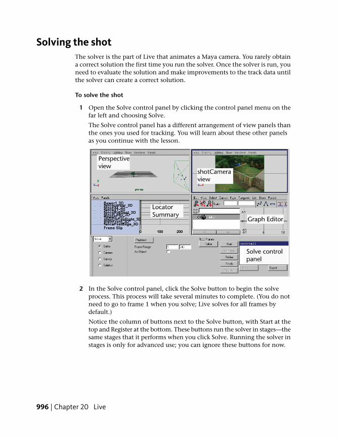
Solving the shotThe solver is the part of Live that animates a Maya camera. You rarely obtaina correct solution the first time you run the solver. Once the solver is run, youneed to evaluate the solution and make improvements to the track data untilthe solver can create a correct solution.
To solve the shot
1 Open the Solve control panel by clicking the control panel menu on thefar left and choosing Solve.
The Solve control panel has a different arrangement of view panels thanthe ones you used for tracking. You will learn about these other panelsas you continue with the lesson.
2 In the Solve control panel, click the Solve button to begin the solveprocess. This process will take several minutes to complete. (You do notneed to go to frame 1 when you solve; Live solves for all frames bydefault.)
Notice the column of buttons next to the Solve button, with Start at thetop and Register at the bottom. These buttons run the solver in stages—thesame stages that it performs when you click Solve. Running the solver instages is only for advanced use; you can ignore these buttons for now.
996 | Chapter 20 Live
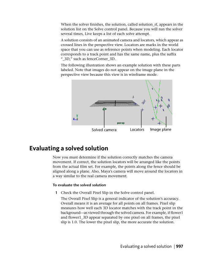
When the solver finishes, the solution, called solution_rf, appears in thesolution list on the Solve control panel. Because you will run the solverseveral times, Live keeps a list of each solve attempt.
A solution consists of an animated camera and locators, which appear ascrossed lines in the perspective view. Locators are marks in the worldspace that you can use as reference points when modeling. Each locatorcorresponds to a track point and has the same name, plus the suffix“_3D,” such as fenceCorner_3D.
The following illustration shows an example solution with these partslabeled. Note that images do not appear on the image plane in theperspective view because this view is in wireframe mode.
Evaluating a solved solutionNow you must determine if the solution correctly matches the cameramovement. If correct, the solution locators will be arranged like the pointsfrom the actual film set. For example, the points along the fence should bealigned along a plane. Also, Maya’s camera will move around the locators ina way similar to the real camera movement.
To evaluate the solved solution
1 Check the Overall Pixel Slip in the Solve control panel.
The Overall Pixel Slip is a general indicator of the solution’s accuracy.Overall means it is an average for all points on all frames. Pixel slipmeasures how well each 3D locator matches with the track point in thebackground—as viewed through the solved camera. For example, if flower1and flower1_3D appear separated by one pixel on all frames, the pixelslip is 1.0. The lower the pixel slip, the more accurate the solution.
Evaluating a solved solution | 997
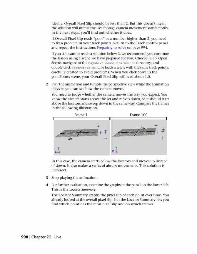
Ideally, Overall Pixel Slip should be less than 2. But this doesn’t meanthe solution will mimic the live footage camera movement satisfactorily.In the next steps, you’ll find out whether it does.
If Overall Pixel Slip reads “poor” or a number higher than 2, you needto fix a problem in your track points. Return to the Track control paneland repeat the instructions Preparing to solve on page 994.
If you still cannot reach a solution below 2, we recommend you continuethe lesson using a scene we have prepared for you. Choose File > OpenScene, navigate to the MayaLiveLessonData/scenes directory, anddouble-click goodPoints.ma. Live loads a scene with the same track points,carefully created to avoid problems. When you click Solve in thegoodPoints scene, your Overall Pixel Slip will read about 1.0.
2 Play the animation and tumble the perspective view while the animationplays so you can see how the camera moves.
You need to judge whether the camera moves the way you expect. Youknow the camera starts above the set and moves down, so it should startabove the locators and sweep down in the same way. Compare the framesin the following illustration.
In this case, the camera starts below the locators and moves up insteadof down. It also makes a series of abrupt movements. This solution isincorrect.
3 Stop playing the animation.
4 For further evaluation, examine the graphs in the panel on the lower left.This is the Locator Summary.
The Locator Summary graphs the pixel slip of each point over time. Youalready looked at the overall pixel slip, but the Locator Summary lets youfind which point has the most pixel slip and on which frames.
998 | Chapter 20 Live

If one point had a very red and yellow graph, you could conclude thatthe point was the source of the problem solution. In this case, manypoints have red and yellow areas, but those areas appear mainly in thefirst 100 frames.
Because red and yellow areas all occur within the first 100 frames, youcan conclude that the solver does not have enough information for thoseframes. To improve the information, you’ll need to add one or more trackpoints for those frames.
How many points you’ll need is not important to fixing this problem.Rather, choosing the right points is what will help the solver. In thefollowing steps, you’ll load another set of points into your scene. Thesepoints will illustrate which types of points to choose.
NOTE The other panels in the layout are the Graph Editor and theshotCamera. The Graph Editor is for advanced users. It can be helpful forexamining the camera animation curves so that you can pinpoint problemareas. The shotCamera panel is useful in later stages, after you have a correctsolution. You can ignore both of these panels for now.
Importing additional tracking dataTo help you improve the solution, we have created another set of track pointsfor you to import.
To import the additional tracking data
1 Choose Track > Import Track Points.
2 Navigate to the MayaLiveLessonData/points directory and double-clickfence_2.txt. Live loads five more track points.
3 Click Solve.
Importing additional tracking data | 999
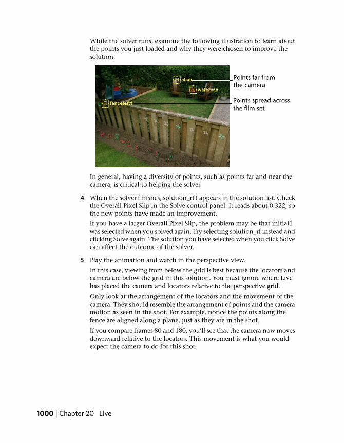
While the solver runs, examine the following illustration to learn aboutthe points you just loaded and why they were chosen to improve thesolution.
In general, having a diversity of points, such as points far and near thecamera, is critical to helping the solver.
4 When the solver finishes, solution_rf1 appears in the solution list. Checkthe Overall Pixel Slip in the Solve control panel. It reads about 0.322, sothe new points have made an improvement.
If you have a larger Overall Pixel Slip, the problem may be that initial1was selected when you solved again. Try selecting solution_rf instead andclicking Solve again. The solution you have selected when you click Solvecan affect the outcome of the solver.
5 Play the animation and watch in the perspective view.
In this case, viewing from below the grid is best because the locators andcamera are below the grid in this solution. You must ignore where Livehas placed the camera and locators relative to the perspective grid.
Only look at the arrangement of the locators and the movement of thecamera. They should resemble the arrangement of points and the cameramotion as seen in the shot. For example, notice the points along thefence are aligned along a plane, just as they are in the shot.
If you compare frames 80 and 180, you’ll see that the camera now movesdownward relative to the locators. This movement is what you wouldexpect the camera to do for this shot.
1000 | Chapter 20 Live
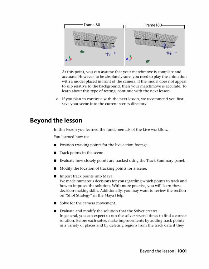
At this point, you can assume that your matchmove is complete andaccurate. However, to be absolutely sure, you need to play the animationwith a model placed in front of the camera. If the model does not appearto slip relative to the background, then your matchmove is accurate. Tolearn about this type of testing, continue with the next lesson.
6 If you plan to continue with the next lesson, we recommend you firstsave your scene into the current scenes directory.
Beyond the lessonIn this lesson you learned the fundamentals of the Live workflow.
You learned how to:
■ Position tracking points for the live-action footage.
■ Track points in the scene
■ Evaluate how closely points are tracked using the Track Summary panel.
■ Modify the location of tracking points for a scene.
■ Import track points into Maya.We made numerous decisions for you regarding which points to track andhow to improve the solution. With more practise, you will learn thesedecision-making skills. Additionally, you may want to review the sectionon “Shot Strategy” in the Maya Help.
■ Solve for the camera movement.
■ Evaluate and modify the solution that the Solver creates.In general, you can expect to run the solver several times to find a correctsolution. Before each solve, make improvements by adding track pointsin a variety of places and by deleting regions from the track data if they
Beyond the lesson | 1001

are not accurate. Even if one track point is off alignment on one frame, itcould result in an incorrect solution.
Your solution has the correct camera movement, but you may wonderwhy the camera and locators are placed below the perspective view grid.If you want to control where the solution is placed within the scene, youneed to give the solver more information, called survey constraints.Continue with the next lesson to learn more.
Exporting and rendering solutions
With the camera movement solved, you can create your animation using thesolved camera to make sure the animation does not move out of the cameraview. If your animators use Maya Complete or another software product, youmust export the camera solution from Live (Scene > Export Scene As). Youcan also export to other 3rd party 3D and compositing applications.
When you render the animation, we recommend you do so without the imageplane background. A better workflow is to render the animation created inMaya separately and then use a compositing software application to combineit with the live footage background.
However, if you do want to render the image plane, you must turn off the UseCache option on the Setup control panel. The Use Cache option utilizes a Rotonode, which does not render. By turning Use Cache off, Live switches to thestandard Maya image plane, which is renderable.
Lesson 2: Solving with survey data
IntroductionThis optional lesson is a continuation of the previous lesson.
The objective in this shot is to replace the filmed fence with a fence modeledin Maya. Suppose you had taken measurements of the fence from the film setand used the measurements to model a fence in Maya. The locators createdby Live would not match the same scale that you used for the model. Also,the locators and camera Live created are not near the perspective view grid,which is a convenient reference for modeling and animating.
To solve these issues, you can incorporate the measurements you surveyedfrom the set into the Live solver. You do this with the survey constraintsfeature.
1002 | Chapter 20 Live
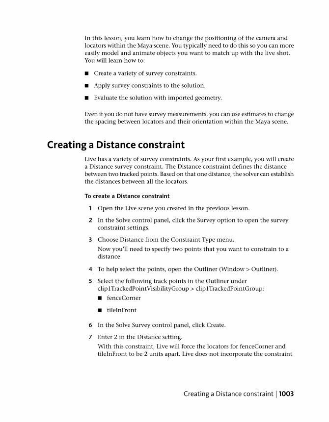
In this lesson, you learn how to change the positioning of the camera andlocators within the Maya scene. You typically need to do this so you can moreeasily model and animate objects you want to match up with the live shot.You will learn how to:
■ Create a variety of survey constraints.
■ Apply survey constraints to the solution.
■ Evaluate the solution with imported geometry.
Even if you do not have survey measurements, you can use estimates to changethe spacing between locators and their orientation within the Maya scene.
Creating a Distance constraintLive has a variety of survey constraints. As your first example, you will createa Distance survey constraint. The Distance constraint defines the distancebetween two tracked points. Based on that one distance, the solver can establishthe distances between all the locators.
To create a Distance constraint
1 Open the Live scene you created in the previous lesson.
2 In the Solve control panel, click the Survey option to open the surveyconstraint settings.
3 Choose Distance from the Constraint Type menu.
Now you’ll need to specify two points that you want to constrain to adistance.
4 To help select the points, open the Outliner (Window > Outliner).
5 Select the following track points in the Outliner underclip1TrackedPointVisibilityGroup > clip1TrackedPointGroup:
■ fenceCorner
■ tileInFront
6 In the Solve Survey control panel, click Create.
7 Enter 2 in the Distance setting.
With this constraint, Live will force the locators for fenceCorner andtileInFront to be 2 units apart. Live does not incorporate the constraint
Creating a Distance constraint | 1003

until you run the solver again and create a new solution. You will do thislater in the lesson.
This constraint is not based on a film set measurement; it is simply anestimate. Using estimates to control the space between locators is oftenuseful, but be careful not to use too many estimates. Too many estimatescan prevent the solver from finding a solution.
Creating a Plane constraintIn addition to the space between locators, you may want them to berepositioned within the scene. For example, you may want the flower locatorsin the solution to rest on top of the perspective view grid, just as the flowersin the shot rest on the ground. In the current solution, the flower locatorsrest below the grid.
A convenient way to bring points onto the grid is to use a Plane constraint,which aligns locators onto a plane.
To create a Plane constraint for the ground
1 Choose Plane from the Constraint Type menu.
2 Select the following track points in the Outliner underclip1TrackedPointVisibilityGroup > clip1TrackedPointGroup:
■ flower1
■ fenceCorner
■ flower2
■ tileInFront
In the shot, these points correspond to points on the ground.
3 Click Create. Live places the Plane constraint on the perspective viewgrid by default.
1004 | Chapter 20 Live
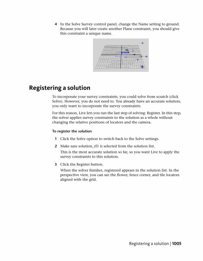
4 In the Solve Survey control panel, change the Name setting to ground.Because you will later create another Plane constraint, you should givethis constraint a unique name.
Registering a solutionTo incorporate your survey constraints, you could solve from scratch (clickSolve). However, you do not need to. You already have an accurate solution;you only want to incorporate the survey constraints.
For this reason, Live lets you run the last step of solving: Register. In this step,the solver applies survey constraints to the solution as a whole withoutchanging the relative positions of locators and the camera.
To register the solution
1 Click the Solve option to switch back to the Solve settings.
2 Make sure solution_rf1 is selected from the solution list.
This is the most accurate solution so far, so you want Live to apply thesurvey constraints to this solution.
3 Click the Register button.
When the solver finishes, registered appears in the solution list. In theperspective view, you can see the flower, fence corner, and tile locatorsaligned with the grid.
Registering a solution | 1005

If you dolly in the view, you’ll also see that the locators for the pointsyou constrained by distance—fenceCorner and tileInFront—are nowabout two grid units apart.
Creating additional Plane constraintsA top view reveals an illogical placement of the fence locators. Instead of beingaligned with the XY plane, they are at an angle. To correct this problem, youneed another Plane constraint that represents the fence.
To create a Plane constraint using the fence locators
1 Click the Survey option to switch to the Survey settings.
2 Make sure the Constraint Type is still set to Plane.
1006 | Chapter 20 Live
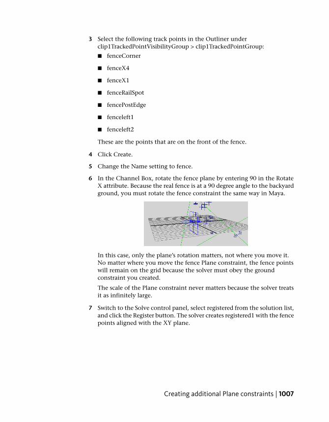
3 Select the following track points in the Outliner underclip1TrackedPointVisibilityGroup > clip1TrackedPointGroup:
■ fenceCorner
■ fenceX4
■ fenceX1
■ fenceRailSpot
■ fencePostEdge
■ fenceleft1
■ fenceleft2
These are the points that are on the front of the fence.
4 Click Create.
5 Change the Name setting to fence.
6 In the Channel Box, rotate the fence plane by entering 90 in the RotateX attribute. Because the real fence is at a 90 degree angle to the backyardground, you must rotate the fence constraint the same way in Maya.
In this case, only the plane’s rotation matters, not where you move it.No matter where you move the fence Plane constraint, the fence pointswill remain on the grid because the solver must obey the groundconstraint you created.
The scale of the Plane constraint never matters because the solver treatsit as infinitely large.
7 Switch to the Solve control panel, select registered from the solution list,and click the Register button. The solver creates registered1 with the fencepoints aligned with the XY plane.
Creating additional Plane constraints | 1007

Evaluating the solution with imported geometryThe best evaluation of your solution is to set an object in front of the solvedcamera and see if it matches the background as you play the animation. Inthis case, we will import a fence modeled in Maya.
Before you load the modeled fence, do the following steps to add one moresurvey constraint. You add a Point constraint to orient the solution sofenceCorner is at the origin. You need fenceCorner at the origin because thefence model has its corner at the origin and you want the two to match exactly.
To reorient the solution with fenceCorner at the origin
1 Switch to the Survey settings.
2 Choose Points from the Constraint Type menu.
3 Select the following track point in the Outliner underclip1TrackedPointVisibilityGroup > clip1TrackedPointGroup:
■ fenceCorner
4 Click Create. Maya creates a Point constraint in your scene, located atthe origin (0,0,0) by default.
5 Switch to the Solve control panel, select registered1 from the solutionlist, and click the Register button. The solver creates registered2 withfenceCorner at the origin.
You will now import a fence that has been modeled to exactly match the fencethat was filmed.
1008 | Chapter 20 Live

To import a modeled fence
1 Choose File > Import.
2 Navigate to the MayaLiveLessonData/scenes directory in the Importbrowse window.
3 Double-click fenceModel.ma to import it.
To evaluate the solution
1 Hide the Plane constraints by selecting them and choosing Display >Hide, Show > Hide Selection By hiding them, you can see the fence better.
2 Enlarge the shotCamera view panel, which is in the upper right of theSolve panel layout. This panel shows the view from the solved Mayacamera.
In frame 1, you can see that the modeled fence accurately matches thefence that was filmed. To quickly see if it matches well in the other frames,you can scrub through the shot in the Time Slider.
3 To scrub through the shot, drag slowly from left to right in the TimeSlider.
The fence model does not appear to slip in relation to the background,so this confirms that the solution is accurate. If you rendered a sequenceof the camera moving around the modeled fence, you could compositethe sequence with the original background and they would exactly match.
Although scrubbing tends to skip frames, it gives a preliminaryconfirmation that the fence model matches the background in all frames.
4 To evaluate the solution in a more accurate playback, select Window >Playblast.
Evaluating the solution with imported geometry | 1009
The Playblast movie is an approximation of how the rendered sequencewill appear. In this movie, you can look for subtle mismatches betweenthe model and the background, such as momentary jitter.
NOTE As an alternative to the Playblast, you could play the animation inMaya, provided you allocate enough memory in the Setup Cache controlpanel. If you have memory allocated for all 240 frames, the playback will beas fast and accurate as the Playblast movie. When using Playblast, you’ll needapproximately 20 Mbytes of free space in your computer’s temporarydirectory.
Beyond the lessonIn this lesson you learned how to apply survey constraints to improve theoverall solution. Survey constraints are useful not only for orienting yoursolution, but also for the initial creation of a solution. In these lessons, yousolved using track data alone. In more complex shots, the solver may failunless you use survey constraints to broaden the information that the solvercan use.
You cannot tell in advance which survey constraints are needed to solve ashot so it is a good idea to plan for some of the survey constraints before youstart tracking. A common example is the Plane constraint, because most shotshave coplanar or approximately coplanar points in them.
Do not add too many estimated survey constraints, as they may conflict witheach other. When you create a Plane constraint for points that are onlyapproximately coplanar, we recommend you turn on Registration Only in theSolve Survey control panel. This option keeps the solver from forcing thepoints to be perfectly coplanar.
Maya Live includes other constraints such as camera constraints and infinitepoints to help with solving. Camera constraints help control the focal length,translation, and rotation of the solved camera. You set them in the Solvecontrol panel Camera settings.
Infinite points are tracked points that you designate as infinitely far from thecamera, such as a cloud, mountain, or any feature in the distant background.Knowing a point is infinite, lets the solver use it exclusively for calculatingcamera movement. Infinite points are helpful for zoom shots, when the camerais static.
For further information and related techniques on Maya Live, refer to theMaya Help.
1010 | Chapter 20 Live
Index
{ } in expressions 641% in expressions 648
2D fluid containercreating 792
3D fluid containercreating 801, 810
3D Paint Tool 610
A
Accuracy 531active rigid body 558Add Attribute button 645Add Attributes 548
for Current Render Type 547Add Dynamic Attributes 548, 645Add Influence 341Add Keys Tool 212Add Per Particle Attribute 548, 645Add Preview Plane 821Add/Edit Contents 792, 797, 811age, particles 549Along Axis 540Alpha Gain 77Amplitude 805animation
curves 206planning, storyboarding 308
Animation Preferences 202Annotation
creating 293description 293
anti-aliasing 458, 515Append to Polygon Tool 105arms
joint chain 324Around Axis 540, 543array
description 548Artisan Erase 612
Assign Edit Textures button 610Assign New Material 467Assign Paint Effects Brush to Hair 783Assign Textures button 618–619assigning a texture map 366Attribute Editor
attribute tabs 65description 65Fur 849viewing 65
Attribute to Paint 610, 618attributes
controlling multiple 631description 37displayed in Attributes list 628linking 631shading 68
audio clips 275Autodesk
technical support 11Web site 11
Automatic Mapping 376applications 376triplanar projection 376
Away From Axis 540, 543Axial Magnitude ramp 949axis indicator 19
B
bald region 843base object
influence object 342base shape
blend shape 359base width 853Bend
hair 764Bend Amount 764Bend Curves Options 764Billow 804
1011 | Index

Billow Density 805birth, particles 549blend modes 611blend shape deformer 352
adding shape to 357editor 353improving deformations 359
blending animation types 231Blinn shading material 441, 443
description 67Blobby Radius Scale, nParticles 965Blur, 3D Paint 617boat locator 825boat wakes 827bones 319Boolean operations 129border edges 84Bounce 925–926Boundary Draw 808Boundary X, Y 796Bounding Box 214braces, in statements 641brackets, double angle 646Break Tangents
Graph Editor 208Bridge 102Browse button 614, 620brush profile 615brushes
3D Paint, Paint Effects 615description 577Kelp 594Mesh 598Teapot 599Thin Line 608
bump, painting 618Buoyancy 826
C
cachefor Live images 985, 1010
cachingnCloth 898–899nParticles 967
caching fluids 800
cameraapplications 496create 496
Camera Attribute Editor 452camera constraints 1010camera tools
Dolly Tool 44overview 43Track Tool 45Tumble Tool 45
camerasanimating 498, 500Film Gate 500undoing changes 498
CanvasClear 568Set Size 568
Canvas Clear 566Caustic Photons 532Caustics
Caustic Photons 527description 519Emit Photons 527light sources 533Photon Intensity 527photon maps 526photons 526
Channel Box 24blend attributes 233, 235description 37hiding, showing 24locking channels 298naming and renaming objects 38transforming and rotating
objects 38translation, rotation, scaling 24
character set 246character setup
description 317Circle 172clear canvas 566clip cycle
description 261clip library 270clip manipulator 258
1012 | Index

clipsapplications 242audio 275blending 274components 245creating 244, 247cycling 261description 239, 242duration 246importing 253inserting 270keyframing 275name 246Outliner 275regular clips 244renaming 248repositioning 250reusing 253scale 246scaling 257source 244, 253Visor 275
cloth texture 446–447Clump Width
hair 772cluster deformer 346cluster handle 348cluster weights 349Collapse 294collapse hierarchy 294Collide Sphere 768Collide Width Scale 926, 928, 960Collision Flag 876–878collision object
fluid 798collisions
nCloth 868–878, 899–900nParticles 925–926, 960
collisions, rigid bodies 554color
Christmas light effect withparticles 648
emitting 797fluid property 792fluid shader 817fur 850
giving object constant color 645giving particles randomly changing
color 646particles 548ramp 549
Color 611color bleeding 515Color Chooser 68, 454Color Feedback
Paint Fur Attributes Tool 846Color Input 804, 817Color Method 797Combine 102components
description 62conditional statements
if 636Conserve attribute 545constraints 554, 880–892
description 291nCloth 881, 886, 908–909orient 296parent 305point 294Point to Surface 881rigid bodies 554
construction history 117, 153, 179container
boundaries 796creating 792, 801, 810resolution 802size 802
Contents Methoddynamic fluid 795Dynamic Grid 794, 797, 812, 816Gradient 803
control object (IK) 290control vertices (CVs) 152
description 63Convert Selection
hair 768converting a UV selection 384Crease Proxy Edge Tool 127creasing
subdivision surface 195
Index | 1013

CreateExpression Editor 628
Create 2D Container 792Create 2D Container with Emitter 793Create 3D Container 802, 810Create Blend Shape 352Create Clip
options 261–262Create Cluster 348Create Constraint 556
hair 768, 785Create Hair 758, 779Create Ocean 820Create Polygon Tool 95Create Ramp 549Create Rest Curves
hair 759creating
constraints 881–886, 908–909liquid simulations 953, 976nCloth 866–868, 895nParticles 918, 920, 931, 933passive collision objects 868, 897
creation expressions 645assigning to rgbPP 645
cross-hair in track box 988cube primitive 21, 78
options 46Curl
hair 773Curl Frequency
hair 773Current Position 759curve
direction 152edit revolved 153start 152
curves, dynamic 753curves, hair 756cutting
subdivision surface 190CV Curve Tool 151cycling a clip 261
D
deforming objects with fluids 800Delete by Type 118Delete Keys 332Delete Region 992Density
description 793emitting 792fluid property 792fur setting 853painting 811
Depth Map Shadows 774, 859Depth Max 805detail
subdivision surface 191Dim Image 377directional light
create 486description 486editing attributes 487
displacementocean 821
Displacementshair 773
displaycreased edges 128only selected object 355Poly Count 129soft and hard edges 124template 60
Display Image 379, 384Display Level 192Display Quality
hair 760–761Display Resolution 452Display Start Position
hair 762Display Unfiltered 387Distance survey constraint 1003Dmap Focus 859Dolly Tool 44
description 44double angle brackets 646Draft rendering setting
description 505
1014 | Index

driven keysdescription 215
duplicatesymmetrical 831
Duplicate Tool 174description 39, 55options 39, 48
Duration 246dynamic attributes
adding 546, 644dynamic curves 777
hair 753dynamic fluid
behavior, changing 794Contents Method 795creating (3D) 810description 791
Dynamic Grid 794, 797, 812, 816Dynamic Properties 892, 895dynamics
definition 535
E
Eccentricity 824Edge Bounded
hair 759edge loop 84
description 84termination 115
edgesborder 84creasing 123hardening 123selecting subdivision surface 193
Edit buttonexpressions 631
Edit Deformers > Blend Shape > Add 357Edit Ramp 553elbow
influence object 341electronic tablet
sculpting surfaces 164else keyword
expressions 640emission rate 924
Emit Fluid Color 798Emit from Object 538emitter, nParticles 918, 931emitters 536
creating 537Omni 538
emittingcolor 797Density 792fluid 792fluid from surface 800
End Bounds 582End Time 202equal to (==) operator 648Equalize
hair 759errors
syntax 637Essential Skills Movies 5
closing the movie window 6playing 6
exiting Maya 27Expression Editor 627expressions 825
advantage of separate 632advantage of single 632creating 628description 625editing 630execution details 633naming conventions 627
Extrude 97extrusion manipulator
subdivision surfaces 189
F
face selection mode 82faces
splitting 107facial animation 344FCheck 462, 553feedback
fur 838fields 536, 553file saving 27
Index | 1015
Fill Object, nParticles 954filmback for Live 983fingernails 193fingers 185Flipbooks 553floating geometry 825Flood 815, 847
Sculpt Geometry Tool 161Flood All 613fluid container
boundaries 793creating 792, 801, 810
fluid dynamics 791fluid properties 792
adding constant values 803emitting 792painting 811
Fluid Slice Location 813fluids
attributes, changing 794color 797deforming geometry with 800emitting 792emitting from surface 800forces 793painting properties 811resolution 802self-shadowing 808shader attributes 803texturing 804
follicleattributes 772hair 754
forcescontainer boundaries 793Gravity 795
Forward Kinematics (FK) 276, 328, 332Four Panes 151Frame In 245Frame Out 245Frame Selection
Graph Editor 206frames per second setting 440Freeze Transformations
description 292Friction 925–926
Fuelpainting 811
Full Crease Edge/Vertex 195Full Res Image 983fur
Attribute Editor 849attributes 838base width 853color modification 850Density 853description 836direction 840Direction Offset 841feedback 838Inclination 853Length 853Paint Attributes Tool 843Polar 841presets 830reduce length 843Roll 841Scraggle 853tip width 853
G
Get Brush icon 615Get Fluid Example 809Getting Started with Maya
about the lessons 2before you begin 3introduction 1lesson conventions 4using lesson files 5using tutorials online 3
Global Illum Photons 509, 514Global Illumination
Accuracy 513color bleeding 515description 501light sources 517photon maps 508photons 508Radius 513rendering process 508, 510
Glue Strength 785
1016 | Index

Go to Bind Pose 340Graph Editor 205
path animation 227Set Driven Key 219tangent modification 228
Gravity 557, 584, 795, 892hair 761, 766
Gravity and Wind 949ground plane 579group nodes
animating 214Group Under 345grouping objects
description 52Growth attributes 605
H
hairassigning a Paint Effects brush 782colliding with objects 782constraining 784creating 758creating Rest curves 765improving playback
performance 761modifying 772Paint Hair Tool 754playing the hair simulation 760rendering 771, 786setting up collisions 767shadowing 774styling 762
Hair Color 783hair curves 756hair system 754
attributes 772Hair to Hair constraint 784–785Hair Width 773hairConstraintShape 785Hairs Per Clump 772hairSystemShape 761Harden Edge 125hardware render 551Hardware Render Buffer 551
Hardware rendererdescription 451
HelpFind Menu 10launching 7
Help resources 5hide layers 844Hide Selection 179hierarchy
about 278collapse 294, 304description 52grouping 52skeleton 319viewing in hypergraph 279
Hinge constraint 556hole
creating subdivision surface 190Hotkeys
brush scale 594description 55setting 55
Hypergraph 53character setup 321description 53overview 53viewing 53viewing hierarchies 53
HypershadeCreate Textures 477description 474rename operation 477
I
if statementsexpressions 634
if-else statementsexpressions 639–640
Ignore Solver Gravity 934IK handles 328
control object 290creating 288creating and animating 329description 288parenting 300
Index | 1017

IK Rotate Plane handle 331IK Solvers
Enable and Disable 340ikSCsolver 289
image cache in Live 985, 1010image plane
description 75importing 76transparency 77
image plane and rendering 1002image size 505, 515, 524Import Clip 253Import Tracked Points 994, 999Incandescence 818Incandescence1 617Inclination 841, 853Incompressibility 961Influence list
Paint Skin Weights Tool 337influence object
smooth skin 340initial orientation
hinge constraint 557Initial State 905–907Input Mesh Attract 902Insert Edge Loop Tool 103, 111Insert Isoparms 168Inverse Kinematics (IK)
description 276, 328limiting motion 298translation limits 304
IPR 619description 451region to be updated 454
IPR Render Current Frame 453Isolate Select 355isoparms 157Iterations
hair 766
J
jawjoint 322
joint chains 319Joint Size 320
Joint Tool 320joints 319
influence on skin 335moving 324
K
Keep Aspect Ratio 610Keep Hard Edge 126Keep Image 507, 525keyframes (keys)
adding 212deleting 211description 200setting 202
keying into a clip 275keys
delete redundant 212Key Selected 314moving 207setting 311
L
Lambert shading material 441–442Layer Editor 834layers
assign objects to 836create 835description 834editor 834hide 844reference 835, 851settings 851template 851
layoutschanging panel layout 32four view layout 39shortcuts 32
Leaf Width Scale attributes 604Leaves attributes 605legs
joint chains 319Length
hair 759
1018 | Index
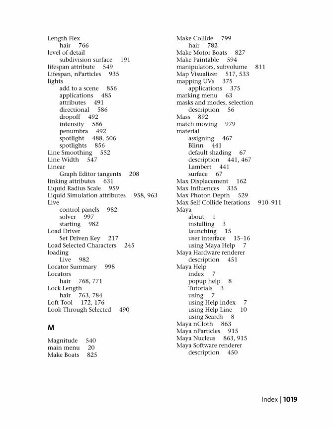
Length Flexhair 766
level of detailsubdivision surface 191
lifespan attribute 549Lifespan, nParticles 935lights
add to a scene 856applications 485attributes 491directional 586dropoff 492intensity 586penumbra 492spotlight 488, 506spotlights 856
Line Smoothing 552Line Width 547Linear
Graph Editor tangents 208linking attributes 631Liquid Radius Scale 959Liquid Simulation attributes 958, 963Live
control panels 982solver 997starting 982
Load DriverSet Driven Key 217
Load Selected Characters 245loading
Live 982Locator Summary 998Locators
hair 768, 771Lock Length
hair 763, 784Loft Tool 172, 176Look Through Selected 490
M
Magnitude 540main menu 20Make Boats 825
Make Collide 799hair 782
Make Motor Boats 827Make Paintable 594manipulators, subvolume 811Map Visualizer 517, 533mapping UVs 375
applications 375marking menu 63masks and modes, selection
description 56Mass 892match moving 979material
assigning 467Blinn 441default shading 67description 441, 467Lambert 441surface 67
Max Displacement 162Max Influences 335Max Photon Depth 529Max Self Collide Iterations 910–911Maya
about 1installing 3launching 15user interface 15–16using Maya Help 7
Maya Hardware rendererdescription 451
Maya Helpindex 7popup help 8Tutorials 3using 7using Help index 7using Help Line 10using Search 8
Maya nCloth 863Maya nParticles 915Maya Nucleus 863, 915Maya Software renderer
description 450
Index | 1019

Maya Vector rendererdescription 451
mayaLive.mll 982mayalive.so 982mental ray for Maya renderer 438, 523
description 451mental ray shaders
assigning to an nParticle outputmesh 972–974
menu sets 20description 20Polygons 72selection 20
Mesh brushesapplications 598attributes 603description 598
meteors 546Mirror Across 322Mirror Geometry 119modeling
description 71, 717polygons 72shaded mode 80symmetry 82types 71
Modify Curveshair 763
modules 20modulus operator (%) 648morphing facial expressions 353motion
speeding up with Graph Editor 209motion capture data
creating clips from 260description 259extending the length of 261redirecting 266
Motion PathAttach to Motion Path 222
motion path animationdescription 220
Motion Streak, nParticles 968move
key points 207objects 35
UVs 384Move and Sew UVs 382Move Snap Settings 85Move Tool 35, 86
N (normal) manipulator 94, 194X, Y, Z manipulator 35
mute track 257, 270
N
nCloth 863caching 898–899Collision Flag 876, 878collision thickness 870, 876collisions 868, 878, 899–900constraints 880, 892, 908–909creating 866, 868, 895Dynamic Properties 892–895Initial State 905, 907Input Mesh Attract 902Mass 892Max Self Collide Iterations 910–911painting properties 902–905Quality Settings 909–911Self Trapped Check 910–911Tangential Drag 893
neckjoints 322
New Matchmove 982new scene 30nodes
description 37initialShadingGroup 66input 66nParticleShape 922Nucleus 922parent 54pivot point 57renaming 54root 54shape 66transform 66
Noisehair 783
non-dynamic fluid 791creating 801
1020 | Index
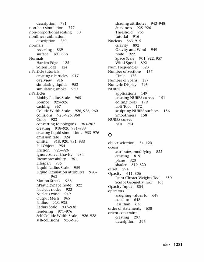
description 791non-hair simulation 777non-proportional scaling 50nonlinear animation
description 239normals
reversing 839surface 160, 838
NormalsHarden Edge 125Soften Edge 124
nParticle tutorialscreating nParticles 917overview 916simulating liquids 953simulating smoke 930
nParticlesBlobby Radius Scale 965Bounce 925–926caching 967Collide Width Scale 926, 928, 960collisions 925–926, 960Color 923converting to polygons 963–967creating 918–920, 931–933creating liquid simulations 953–976emission rate 924emitter 918, 920, 931, 933Fill Object 954Friction 925–926Ignore Solver Gravity 934Incompressibility 961Lifespan 935Liquid Radius Scale 959Liquid Simulation attributes 958–
963Motion Streak 968nParticleShape node 922Nucleus nodes 922Nucleus wind 949Output Mesh 965Radius 923, 935Radius Scale 937–938rendering 971–976Self Collide Width Scale 926–928self-collisions 926–928
shading attributes 943–948Stickiness 925–926Threshold 965tutorial 916
Nucleus 863, 915Gravity 892Gravity and Wind 949node 922Space Scale 901, 922, 957Wind Speed 892
Num Frequencies 823Number of Sections 157
Circle 172Number of Spans 157Numeric Display 795NURBS
applications 149creating NURBS curves 151editing tools 179Loft Tool 172sculpting NURBS surfaces 156Smoothness 158
NURBS curveshair 754
O
object selection 34, 120ocean
attributes, modifying 822creating 819plane 820shader 819–820
offset 294Opacity 611, 806
Paint Cluster Weights Tool 350Sculpt Geometry Tool 163
Opacity Input 804operators
assigning values to 648equal to 648less than 636
order of statements 638orient constraint
creating 297description 296
Index | 1021

origin 18orthographic view 43Outliner 244, 248, 275, 859
description 153, 178parenting objects 178placing clips from 254
Outputhair 754
Output Mesh, nParticles 965Output window 457Overall Pixel Slip 997Oversample 771Oversample Post Filter 771
P
paint brushesblending 572
Paint Effects3D objects 589, 593applications 607Brush Settings window 617brushes, 3D Paint 615making surfaces paintable 594panel 587
Paint Effects hair 754, 771Paint Effects to Polygons 601Paint Fluids Tool 811Paint Fur Attributes Tool 843
Color Feedback 846Flood 847Reflection 848Smooth operation 847
Paint Hair Tool 754Paint Selection Tool 83, 347Paint Skin Weights Tool 337Paint Weight Menu 338painting
2D strokes 5643D strokes 5753D strokes in scene view 579bump 618Density 811fluid properties 811Fuel 811interactively 618
pressure sensitivity 576strokes 577Temperature 816UV preparation 621
pairBlend attribute 236panel 18panel layout 509, 522parent constraint
description 305weighting 308
parent node 54parenting
description 285particle attributes, per object and per
particle 548particle object 538particles
applications 535changing form of 545description 536render type 545streaks 546
passive collision object 868, 897, 920, 956
Passive Fillhair 759
path animationblending 231description 220position marker 226Twist attribute 230UValue 224
per object attributes 548Per Particle (Array) Attributes 645per particle attributes 548
how to distinguish 548Perlin Noise 804perspective view 43Photon Intensity 509, 512, 530photon maps 526, 533
description 508visualizing 517
Photon Refractions 529photons
Accuracy 531Caustic Photons 532
1022 | Index
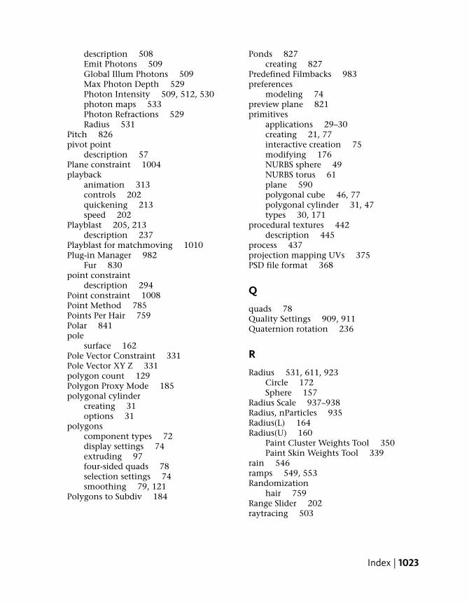
description 508Emit Photons 509Global Illum Photons 509Max Photon Depth 529Photon Intensity 509, 512, 530photon maps 533Photon Refractions 529Radius 531
Pitch 826pivot point
description 57Plane constraint 1004playback
animation 313controls 202quickening 213speed 202
Playblast 205, 213description 237
Playblast for matchmoving 1010Plug-in Manager 982
Fur 830point constraint
description 294Point constraint 1008Point Method 785Points Per Hair 759Polar 841pole
surface 162Pole Vector Constraint 331Pole Vector XY Z 331polygon count 129Polygon Proxy Mode 185polygonal cylinder
creating 31options 31
polygonscomponent types 72display settings 74extruding 97four-sided quads 78selection settings 74smoothing 79, 121
Polygons to Subdiv 184
Ponds 827creating 827
Predefined Filmbacks 983preferences
modeling 74preview plane 821primitives
applications 29–30creating 21, 77interactive creation 75modifying 176NURBS sphere 49NURBS torus 61plane 590polygonal cube 46, 77polygonal cylinder 31, 47types 30, 171
procedural textures 442description 445
process 437projection mapping UVs 375PSD file format 368
Q
quads 78Quality Settings 909, 911Quaternion rotation 236
R
Radius 531, 611, 923Circle 172Sphere 157
Radius Scale 937–938Radius, nParticles 935Radius(L) 164Radius(U) 160
Paint Cluster Weights Tool 350Paint Skin Weights Tool 339
rain 546ramps 549, 553Randomization
hair 759Range Slider 202raytracing 503
Index | 1023

Redirect Tool 266creating redirect control 266keyframing control 268positioning control 267
reduce fur length 843reference layer 835, 851Refine Selected Components 194, 196reflect
Paint Fur Attributes Tool 848Reflection
Sculpt Geometry Tool 165Reflection X 612refractions
Max Trace Depth 529photon refraction 529refraction levels 529
Register step 1005renaming clips 248renaming surfaces 833render a scene 860Render Current Frame 585render image plane 1002Render Sequence 552Render Settings 458, 504, 860render types, setting for particles 545Render View 451, 523, 619
Keep Image 507, 525rendering
anti-aliasing 515batch rendering 459, 464compositing layers 464description 437hardware 438, 464image size 505, 515methods 438overview 439panel layout 509, 522raytracing 503render settings 504sampling 516shading surfaces 466shadows 506software 438, 450view region to be rendered 452
rendering nParticles 971, 976rendering particles 553
ReplacePaint Cluster Weights Tool 350
resolution, fluid 802Rest Position 759Retain component spacing 85return to start time 202reusing clips 253reverse normals 839Revolve Tool 150
creating surfaces 153editing surfaces 153
rewind 202rgbPP attribute 548
use in expressions 645ribs
joints 324–325ridges
subdivision surface 195rigid bodies 554
active 558applications 535collisions 554constraints 554passive 558
rigid skinning 343Roll 826, 841root
skeleton 327root node 54Rotate Tool
description 36X, Y, Z manipulator 36X, Y, Z, manipulator 90
Rotate UVs 385rotating objects
options 50rotInterpolation 236runtime expressions 646
assigning rgbPP in 647
S
sampling 516Save As 609Save Scene 27saving files 27, 40, 59
1024 | Index
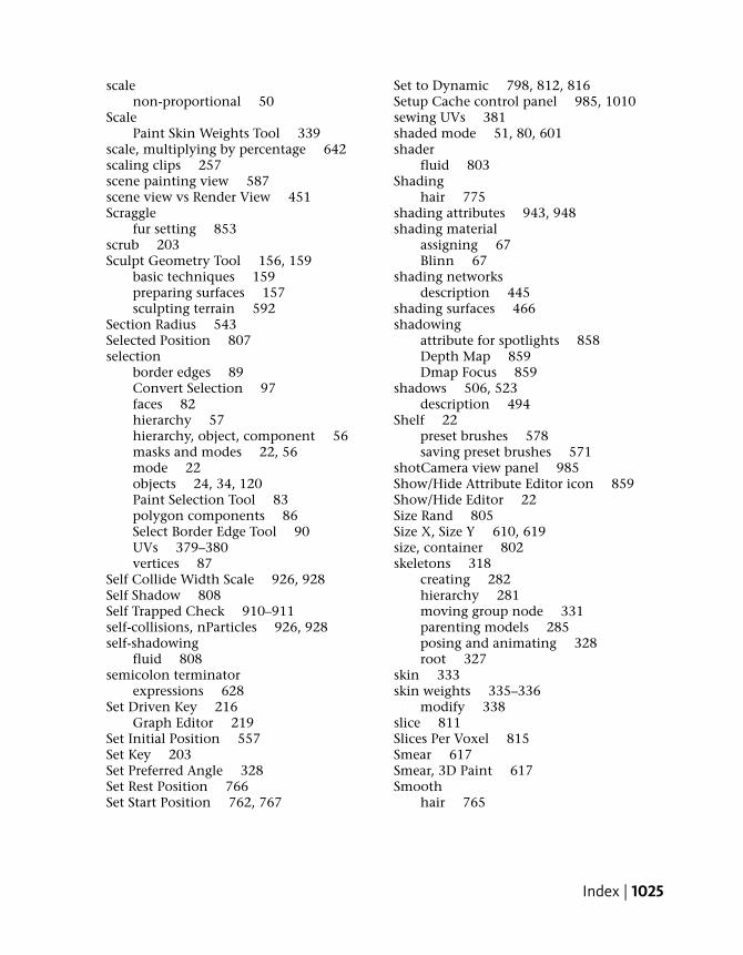
scalenon-proportional 50
ScalePaint Skin Weights Tool 339
scale, multiplying by percentage 642scaling clips 257scene painting view 587scene view vs Render View 451Scraggle
fur setting 853scrub 203Sculpt Geometry Tool 156, 159
basic techniques 159preparing surfaces 157sculpting terrain 592
Section Radius 543Selected Position 807selection
border edges 89Convert Selection 97faces 82hierarchy 57hierarchy, object, component 56masks and modes 22, 56mode 22objects 24, 34, 120Paint Selection Tool 83polygon components 86Select Border Edge Tool 90UVs 379–380vertices 87
Self Collide Width Scale 926, 928Self Shadow 808Self Trapped Check 910–911self-collisions, nParticles 926, 928self-shadowing
fluid 808semicolon terminator
expressions 628Set Driven Key 216
Graph Editor 219Set Initial Position 557Set Key 203Set Preferred Angle 328Set Rest Position 766Set Start Position 762, 767
Set to Dynamic 798, 812, 816Setup Cache control panel 985, 1010sewing UVs 381shaded mode 51, 80, 601shader
fluid 803Shading
hair 775shading attributes 943, 948shading material
assigning 67Blinn 67
shading networksdescription 445
shading surfaces 466shadowing
attribute for spotlights 858Depth Map 859Dmap Focus 859
shadows 506, 523description 494
Shelf 22preset brushes 578saving preset brushes 571
shotCamera view panel 985Show/Hide Attribute Editor icon 859Show/Hide Editor 22Size Rand 805Size X, Size Y 610, 619size, container 802skeletons 318
creating 282hierarchy 281moving group node 331parenting models 285posing and animating 328root 327
skin 333skin weights 335–336
modify 338slice 811Slices Per Voxel 815Smear 617Smear, 3D Paint 617Smooth
hair 765
Index | 1025
Paint Fur Attributes Tool 847Paint Skin Weights Tool 339
Smooth Bind 335Smooth Shade All 80, 441smooth skin 335
influence object 340unnatural deformation 336
smoothing polygons 79, 121Snap Mode 22
Snap to Grid 85Snap to Points 173
Soft Modification Tool 130Soften Edge 124Software renderer
description 450software rendering 450solo track 256Solve control panel 996solver for Live 997source clip 244Source In 246Source Out 246Space Scale 901, 922, 957spans, displaying 158Specular
hair 775Specular Power
hair 775Specularity 824sphere primitive 49
options 63sphrand function, use with random
color 647spinal column
joint chain 322spine
parenting arms and legs 327Split Polygon Tool 107spotlight
aiming 489Cone Angle 492description 488
spotlights 856Spottyness 805Stamp Depth (3D) 816Stamp Spacing 615
Standard Mode 191Start Position 759
setting 762Start Track button 988starting Maya 15statements
expression order 638static channels
remove 212Static Grid 816Status Line 20–21
expanding and collapsing items 22Stickiness 925–926Stiffness
hair 761, 766Stiffness Scale
hair 766Streak render type 546stroke
attributes 581attributes, Global Scale 583attributes, Gravity 584attributes,Turbulence 595description 577Stroke Refresh 588
strokesdeleting 596polygon conversion 601rendering 584, 597, 600tubes 580
Stylus Pressure 164, 576, 611Sub Segments
hair 772Subdiv Proxy
Crease Proxy Edge Tool 127description 121toggle display 123using 122
subdivision surfacesconverting polygons 183cutting 190Extrude Face 187extrusion manipulator 189selecting faces 187selecting vertices 189Split Polygon Tool 185
1026 | Index
subvolume manipulators 811summary track
description 255surface
material 67normals 160pole 162
surface render 800surfaces normals 838survey constraints 1002, 1010Survey option 1003symmetry 82syntax, errors 637
T
Tail Fade 547Tail Size 547Tangent
Graph Editor 214handles in Graph Editor 208
Tangential Drag 893target
blend shape 352Temperature
fluid property 792painting 816
template brushdescription 566, 578modifying settings 566resizing 566
template display 60, 319applications 60description 60untemplating objects 65
template layer 851Test Render 551texture map
applications 361assigning 366description 361procedural 442UVs 363
Texture Opacity 804Texture Scale 805Texture Time 809
Texture Type 804textures
cloth 446–447interactive 3D placement 480procedural 445
texturing, fluid 804The Art of Maya 3Thickness 870–876Thinning
hair 772Threshold, nParticles 965ticks
red key 203time
expressions 635predefined variable 628value at different frames 628
Time option 440Time Slider 202time warps 275tip width 853Toggle Texture Borders 383
applications 383Tool Settings 609Toolbox 32
transformation tools 34, 85torus
options 61track 245
description 245muting 257soloing 256view area 246
track box tool 986Track control panel 984track point 984Track Summary panel 989Track Tool 45
description 45Tracking Direction 988transform nodes
not used for particle expressions 645transparency, skin 335Trax Editor
character sets 246clip library 270
Index | 1027

clip manipulator 258cycling a clip 264Graph Anim Curves 252Load Selected Characters 245motion capture data 259mute track 257Offset attribute 265panel layout 241repositioning clips 250scaling clips 257solo track 256summary track 255time warps 275Toolbar 247track 245
triplanar projection 376tubes
attributes 604Creation 599editing attributes 570Flower 599Leaves 599
Tumble Tooldescription 45
turbulence 795Turbulence
options 595Twist 331
hair 764Twist attribute 230Two Panes Stacked 619
U
U Counthair 759
UI Elements 609undo 37, 592Update on Stroke 620Use Cache option 1002Use Depth Map Shadows 491, 495user interface 15–16user preferences
restoring 12saving 11
UV Texture Editorapplications 371converting a selection 384description 371Dim Image 377Display Image 379, 384Display Unfiltered 387Move and Sew UVs 382Rotate UVs 385Toggle Texture Borders 383viewing UVs 373
UVsAutomatic Mapping 376description 363image range 373–374mapping 375modifying 379moving 384preparing for painting 621projection mapping 375selecting 379–380sewing 381shells 382viewing 371, 373
V
V Counthair 759
ValuePaint Cluster Weights Tool 350
Vector rendererdescription 451
velocitycontrolling in particles 545
Velocity, fluid property 792vertices
subdivision surface 189–190viewing rendered frames 462viewing shaded objects 51views
orthographic 43perspective 43shaded 51wireframe 54
1028 | Index
Visor 244, 275description 254placing clips from 254preset brushes 577, 593
volume axis field 539Volume Axis field 940–942volume pixels 794Volume Shape 539voxels 794, 802
W
Wakescreation 827
wateropen 819
Wave Length Max 823
Wave Peaking 823Wind Speed 892Wireframe on Shaded mode 80workspace 17world space coordinates 93
X
X-Ray 81, 335X, Y, Z
axes 19axis indicator 19origin 18
X, Y, Z Resolution 802X, Y, Z Size 802X, Z ground plane 579
Index | 1029

1030


![Skaffold - storage.googleapis.com · [getting-started getting-started] Hello world! [getting-started getting-started] Hello world! [getting-started getting-started] Hello world! 5.](https://static.fdocuments.in/doc/165x107/5ec939f2a76a033f091c5ac7/skaffold-getting-started-getting-started-hello-world-getting-started-getting-started.jpg)