May 9, 2005 Andrew C. Gallagher1 CRV2005 Detection of Linear and Cubic Interpolation in JPEG...

May 9, 2005 Andrew C. Gallagher1 CRV2005

Detection of Linear and Cubic Interpolation in JPEG

Compressed ImagesAndrew C. Gallagher

Eastman Kodak [email protected]


The Problem• An image consists of a number of

discrete samples. • Interpolation can be used to modify the

number of and locations of the samples.• Given an image, can interpolation be

detected? If so, can the interpolation rate be determined?


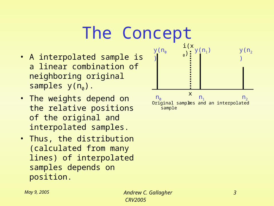
The Concept• A interpolated sample is a

linear combination of neighboring original samples y(n0).

• The weights depend on the relative positions of the original and interpolated samples.

• Thus, the distribution (calculated from many lines) of interpolated samples depends on position.

Original samples and an interpolated samplen0 n1 n2

y(n0

)y(n1) y(n2

)

x0

i(x0

)


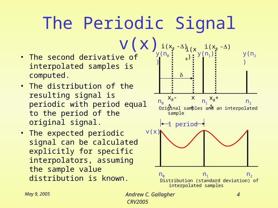
The Periodic Signal v(x)• The second derivative of

interpolated samples is computed.

• The distribution of the resulting signal is periodic with period equal to the period of the original signal.

• The expected periodic signal can be calculated explicitly for specific interpolators, assuming the sample value distribution is known.

n0 n1 n2

y(n0

)y(n1) y(n2

)

x0

i(x0

)

x0-

i(x0 -)

x0+

i(x0 -)

Original samples and an interpolated sample

n0 n1 n2Distribution (standard deviation) of

interpolated samples

1 period

v(x)


The Periodic Signal v(x)• Linear Interpolation • Cubic Interpolation

This property can be exploited by an algorithm designed to detect linear interpolation.


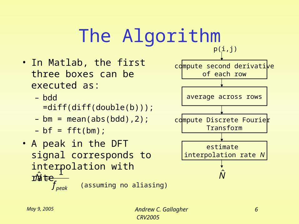
The Algorithm• In Matlab, the first

three boxes can be executed as:– bdd

=diff(diff(double(b)));– bm = mean(abs(bdd),2); – bf = fft(bm);

• A peak in the DFT signal corresponds to interpolation with rate

compute second derivativeof each row

p(i,j)

average across rows

compute Discrete Fourier Transform

estimate interpolation rate N

N̂peakf

N1ˆ

(assuming no aliasing)


Resolving Aliasing• The algorithm produces samples of the periodic

signal v(x). • Aliasing occurs when sampled below the Nyquist

rate (2 samples per period). • All interpolation rates

will alias to N. • Only two possible solutions for rates N>1

(upsampling). An infinite number of solutions for N<1.

• The correct rate can often be determined through prior knowledge of the system.

1

NQN

NA (Q a positive integer)


Example Signals: N = 2A

fter

sum

min

gacr

oss

row

s v(x

) A

fter

com

puti

ng D

FT


Example DFT Signals


Effect of JPEG Compression

• Heavy JPEG compression appears similar to an interpolation by 8.

• Therefore, the peaks in the DFT signal associated with JPEG compression must be ignored.

digital zoom by N

o(i,j)

JPEG compression

p(i,j) Aft

er

com

puti

ng D

FT no interpolationJPEG compression

interpolation N = 2.8JPEG compression


Experiment• A Kodak CX7300 (3MP) captured 114

images • 13 images were non-interpolated. The

remainder were interpolated with rate between 1.1 and 3.0.

N


Results• Algorithm correctly classified between

interpolated (101) and non-interpolated (13) images.

• Interpolation rate was correctly estimated for 85 images.

• For the remaining 16 images, the algorithm identified the interpolation rate as either 1.5 or 3.0. This is correct but ambiguous.


Conclusions• Linear interpolation in images can be

robustly detected. • The interpolation detection algorithm

performs well even when the interpolated image has undergone JPEG compression.

• The algorithm is computationally efficient. • The algorithm has commercial applications

in printing, image metrology and authentication.

May 9, 2005 Andrew C. Gallagher1 CRV2005 Detection of Linear and Cubic Interpolation in JPEG...

Documents

Transcript of May 9, 2005 Andrew C. Gallagher1 CRV2005 Detection of Linear and Cubic Interpolation in JPEG...