May 21, 2003 (Edited by World Bank) Case 4. Evaluation of ...
58
4-1 May 21, 2003 (Edited by World Bank) Case 4. Evaluation of Investments for the Expansion of an Electricity Distribution System Glenn P. Jenkins and Henry B.F. Lim * The Comission Federal de Electricidad (CFE), Mexico’s national electric utility, generates, transmits and distributes electricity to the whole country. During the oil boom of the 1970s, CFE was able to make sufficient investments in the power sector to meet the 6 to 7 percent annual growth in demand; however, when the price of oil fell in the 1980s, investments in the power sector were greatly reduced and the power system deteriorated throughout the decade. By 1989, conditions had reached a point where substantial investments had to be made or the system’s reliability would suffer badly. The power system might even fail to meet new demand, resulting in power shortages. In the power distribution area, the focus of this case study, the deferred investment caused overloading of the distribution substations which resulted in substantial energy losses and power failures. New transformer substations and distribution equipment were needed to mitigate these problems. In addition, during 1990-94, as the monopoly provider of electricity, CFE had to install additional substations, distribution lines, hookups, and meters to provide electricity to about 700,000 new customers each year. More than 1 million customers were illegally connected to the power supply. This pilfering of electricity became a severe financial drain on CFE. About 1 million meters were needed to eliminate this financial loss, along with increased efforts to detect pilferage. CFE also faced problems in relation to the efficiency of billing and collection from its metered customers, * This study has benefited greatly from the assistance of a number of people. Alfred Thieme was a constant source of advice and encouragement. Nisangul Ceran and Luis E. Gutierrez spent much time to provide us with essential information from the World Bank’s archives and to give us a better understanding of the electricity sector in Mexico. The collaboration of our colleagues, Alberto Barreix, Migara Jayawardena, Chun-Yan Kuo, Mario Marchesini, Raghavendra Narain and Harmawan Rubino Sugana was, as always, helpful and greatly appreciated. Any errors and omissions that remain are our responsibility.
Transcript of May 21, 2003 (Edited by World Bank) Case 4. Evaluation of ...

4-1
May 21, 2003 (Edited by World Bank)
Case 4. Evaluation of Investments for the Expansion of an
Electricity Distribution System
Glenn P. Jenkins and Henry B.F. Lim∗⋅
The Comission Federal de Electricidad (CFE), Mexico’s national electric utility, generates,
transmits and distributes electricity to the whole country. During the oil boom of the 1970s, CFE
was able to make sufficient investments in the power sector to meet the 6 to 7 percent annual
growth in demand; however, when the price of oil fell in the 1980s, investments in the power
sector were greatly reduced and the power system deteriorated throughout the decade. By 1989,
conditions had reached a point where substantial investments had to be made or the system’s
reliability would suffer badly. The power system might even fail to meet new demand, resulting
in power shortages.
In the power distribution area, the focus of this case study, the deferred investment caused
overloading of the distribution substations which resulted in substantial energy losses and power
failures. New transformer substations and distribution equipment were needed to mitigate these
problems. In addition, during 1990-94, as the monopoly provider of electricity, CFE had to install
additional substations, distribution lines, hookups, and meters to provide electricity to about
700,000 new customers each year.
More than 1 million customers were illegally connected to the power supply. This
pilfering of electricity became a severe financial drain on CFE. About 1 million meters were
needed to eliminate this financial loss, along with increased efforts to detect pilferage. CFE also
faced problems in relation to the efficiency of billing and collection from its metered customers,
∗⋅This study has benefited greatly from the assistance of a number of people. Alfred Thieme was a constant source of advice and encouragement. Nisangul Ceran and Luis E. Gutierrez spent much time to provide us with essential information from the World Bank’s archives and to give us a better understanding of the electricity sector in Mexico. The collaboration of our colleagues, Alberto Barreix, Migara Jayawardena, Chun-Yan Kuo, Mario Marchesini, Raghavendra Narain and Harmawan Rubino Sugana was, as always, helpful and greatly appreciated. Any errors and omissions that remain are our responsibility.

4-2
and needed new computers and training to help redress this problem. Finally, it had to improve
its routine repair and maintenance services to reduce substations’ down time.
To address all these issues, CFE, made plans to undertake 14 separate investments
costing a total of Mex $ 5,926 billion or US$ 1.93 billion in 1990 prices. The project was to be
completed in five years, from 1990 to 1994. This study evaluates these investments from both the
financial and economic points of view using data available before the project was implemented.
Distribution projects have usually been treated as a required technical part of a power system,
and their specific costs and benefits have often been overlooked. As electricity systems are
becoming unbundled through privatization, the traditional methods of appraising electricity
distribution investments must change. The purpose of this study is to develop and illustrate a
complete methodology that considers the financial, economic, stakeholder and risk aspects of
such investments.
The financial analysis ascertains the project’s financial feasibility and determines whether
it will be a financial drain on the utility. The economic analysis evaluates the project from the
public’s or the economy’s point of view. It looks at both the benefits and costs of the project
differently from the financial analysis. For instance, a power project may be financially profitable
because of its heavily subsidized fuel price. The economic analysis will evaluate the fuel price at
its economic opportunity cost and therefore expose the true net economic value of the project.
Another example would be when the capital cost of a project is highly subsidized because a state-
owned utility is carrying it out. This often leads to over investment in the sector and the use of
overly capital-intensive technology (Jenkins 1985). The study also includes a stakeholder
analysis that attempts to allocate the project’s net economic benefits or externalities to various
groups that gain or lose from the project. These groups usually include the producers, the various
classes of consumers, the workers, the low income groups, the government, and society at large.
This study also estimates the project’s poverty alleviation impact.
The environmental costs of a project that are externalized in the financial analysis are
internalized in the economic analysis. For some projects, the environmental costs, such as the
costs of decommissioning a nuclear power plant, may critically affect its net economic benefits.

4-3
Mexico has two public electric utilities. CFE is the major electric utility. A second minor
utility, Compania de Luz y Fuerza del Centro, formerly a private utility and now wholly-owned
by CFE, is responsible for electricity distribution in the area of Mexico City and vicinity.
During the 1970s, during Mexico’s oil boom, investment in the power sector was a
sizable 13 percent of gross public investment. The economic crisis of the following decade led
the government to reduce CFE’s annual investment from US$2 billion (real 1989 prices) to
US$1.4 billion in 1988, a reduction of 30 percent. The investment restrictions imposed on CFE
forced the company to postpone its program to expand its generation, transmission and
distribution capacity. Although these restrictions did not have a significant negative effect on the
quality of service as of 1989, the company expected that quality would suffer in the not too
distant future, affecting the reliability of electricity supplies. To correct this situation, the
Mexican government decided to implement a 10-year investment program the Programa de
Obras e Inversiones del Sector Electrico 1989.
At the end of 1988 CFE’s installed capacity was 23,921 megawatts (MW) of generation
plants, 56,000 kilometers of high voltage transmission lines (400, 230, and 115 kilovolts),
255,000 kilometers of distribution lines, and 16,500 (MVA) of distribution transformers.
Although most of the country is interconnected through high-voltage transmission lines, full
exchange of power plant reserves is not possible because of limited interconnections among
different regions.
CFE expected that electricity sales would grow at 6.6 percent per year during 1988-98.1
Should demand grow more rapidly and investment in the power sector remain stagnant, the
reliability of the power supply would deteriorate, eventually leading to a shortage situation.
Consequently, as part of the 10-year investment program, CFE prepared four subprograms to be
implemented over five-years address specific problems in the areas of generation, transmission,
distribution, and rehabilitation of old thermal plants.
1 Estimated using an econometric model that assumed that the population would grow at an average of 2.16 percent per year during the period, real public investment would grow at 8.7 percent per year and real gross domestic product at 5.1 percent per year.

4-4
During 1989-98, CFE planned to add 17,626 MW in new power plants, of which 3,207
MW would be hydroelectric plants. The “subprogram to rehabilitate thermoelectric plants”
would renovate older thermoelectric power plants to improve their thermal efficiency and
availability. The transmission subprogram would expand and improve transmission installations
rated 115 to 400 kilovolts. Finally, the distribution subprogram was designed to:
• Reduce the distribution system’s power losses,
• Supply new customers with connections,
• Curtail electricity pilferage,
• Improve the system’s reliability by reducing power outages,
• Improve management, accounting and bill-collection efficiency by installing new
computers,
• Improve the maintenance of the distribution system through training and the purchase of
vehicles.
Project Description
In 1988 the total demand as recorded at substations was 10,982 MW. At the projected level of
demand growth, existing capacity would be insufficient to meet demand by 1994. To overcome
that shortfall, by means of this project CFE planned to add 2,080 MVA of new capacity to 109
substations, install 1,250 MVA in distribution transformers, construct 18,000 kilometers of
secondary feeders and make 700,000 new connections per year during the five-year investment
period.
In addition to reducing technical losses, the project would address the problem of
nontechnical losses. In the past CFE maintained a collection cycle of 60 days for its electricity
bills and had reduced uncollected accounts to only 0.1 percent of total billings. However, its
collection system deteriorated because of an increase in tariff complexity. The project design
includes a component to improve collection and administrative efficiency collection by setting up
665 computer billing stations. In addition, as of December 1988, 1,044,000 (or about 7 percent)

4-5
of total customers were connected directly to the distribution lines without a meter. To address
this problem, the project includes the purchase and installation of 1 million new meters.
The total investment cost of the project is Mex$5,926 billion, or US$1,930 million in
1990 prices. Table 4.1 summarizes the project’s components and costs.
Table 4.1. Project Subprograms and Costs
(Mex$ millions, 1990 prices)
Activity Cost
Substation improvements 722,214
Subtransmission lines 237,874
Primary feeders 70,378
Supervisory control equipment 50,454
Distribution lines 427,923
Capacitors 160,034
Reclosing equipment 356,512
Secondary network improvement 1,004,611
Voltage regulators 19,300
Vehicles and equipment 660,618
Metering equipment 911,893
Computer equipment 83,335
Other equipment 67,885
Buildings 349,807
Maintenance 521,421
Rural electrification 281,561
Total 5,925,820
a. Equivalent to US$1,930 million in 1990 prices.
Source: World Bank (1990), “Mexico Transmission and Distribution Project,” Staff Appraisals Report No. 8197-ME, Washington, D.C., USA.
The project’s financing comes from both foreign and domestic sources. Foreign funds,
amounting to US$704.4 million, are mainly from multinational development agencies, export
credit agencies and suppliers. Table 4.2 summarizes the sources of funds.

4-6
Table 4.2. Project Financing
(1990 US$ millions)
Source Local Foreign Total World Bank Loan n.a. 162 162 Inter-American Development Bank Loan n.a. 151.8 151.8 Eximbank Japan n.a. 28.5 28.5 Bank's hydroelectric project n.a. 25.2 25.2 Turnkey contracts n.a. 106.4 106.4 Suppliers' credits n.a. 230.4 230.4 Consumers’ contributions 29.3 n.a. 29.3 Government contributions 38.8 n.a. 38.8 CFE 1,157 n.a. 1,157 Total 1,225.1 704.4 1,930
n.a. Not applicable.
Source: World Bank (1990), “Mexico Transmission and Distribution Project,” Staff Appraisals Report No. 8197-ME, Washington, D.C., USA.
Sources of Incremental Financial and Economic Benefits
Financial Benefits
The project has four main sources of financial benefits.
One objective of this project was to expand access to electricity in both urban and rural
areas. Starting in 1990, CFE planned to provide connections to 700,000 new customers each
year. Hence a source of financial benefits is the incremental sales from increased electricity
consumption arising from new connections to customers previously without electricity.
Financial benefits will also arise from the cost savings derived from reduced technical
losses at distribution substations. A distribution network faces different types of technical losses,
ranging from transformer and subtransmission line losses to maintenance and outage losses. As
the installation of new distribution lines is mainly to provide connections for new customers, we
shall assume that the project did not have much impact on line losses. The major technical losses
are transformer losses and outage losses.

4-7
In 1988, demand at the distribution system’s substations was 10,982 MW. The increase of
2080 MVA in substation capacity and the addition of 1250 MVA of new transformers will
reduce the demand factor of some transformers from 118 to 98 percent.2 This will reduce the
level of technical losses, which translates into fuel and capacity savings for the utility.
When the meters are installed, some consumers who previously pilfered electricity will
reduce their demand for electricity, and the utility will no longer have to provide this electricity.
CFE will benefit financially from the resulting savings in capacity and fuel.
A large increase in financial revenue will come from incremental sales brought about by
the reduction in nontechnical losses, namely, improved billing and collection and the metering of
1 million previously unmetered customers. In 1988 some 1,044,000 customers were connected to
the system, but lacked meters. During 1990–94, 200,000 meters per year were to be installed for
these customers. With new computer systems and training, the efficiency of the accounting
departments will be improved. We assume that the billing cycle will be reduced to one month
and the amount of uncollected bills will be reduced to 0.1 of a month’s billings per year.
The lack of investment in the distribution network has affected the quality of service to
customers. One of the objectives of this project is to reduce total outage time by 12, 29, 55, 97,
and 136 minutes each year, respectively, from 1990 to 1994 (Gutierrez 1991, p.8). The reduction
in outages means that CFE can sell more electricity during any given period, yielding additional
revenue. The net financial benefit to CFE will be the additional revenue less the extra fuel cost
required to generate this additional supply.
Economic Benefits
The economic impacts of this project will derive from the following five areas:
• Additional consumption from new connections
• Fuel and capacity savings from the reduction in transformer losses
• Increased consumption because of the reduction in outages
2 Demand factor is defined as the demand at the transformer divided by the transformer’s rated capacity.

4-8
• Curtailment of that part of electricity consumption previously pilfered by unmetered
customers, which will be a loss to the consumers but a fuel saving to the economy
• An environmental impact that mainly includes the land area used for distribution lines
and substations.
Financial Analysis
Assumptions
For the purpose of the financial analysis, we made the following assumptions:
• Tariff Policy. Several proposals for the financial reform of CFE have been suggested. One
such proposal is for CFE to achieve a 7 percent real return on new assets. Another is to
set electric tariffs on all energy to cover its long-run marginal costs (LRMC). This study
has incorporated the 7 percent return on new assets proposal through the use of a 7
percent real return on equity. In 1988 the ratio of the net of tax electric tariff to the
marginal cost of electricity supply for different customer groups ranged from 14 percent
for rural (agriculture) customers to 81 percent for commercial customers (table 4.3). In
this study we incorporate the proposal to equate power prices with marginal costs through
the use of a tariff adjustment mechanism (for a more complete discussion see the
sensitivity analysis of the financial analysis).

4-9
Table 4.3. Average Electricity Tariffs and LRMC (1988 US$ millions/kWh)
Consumer Tariff (net of tax)
LRMC Price/LRMC ratio (%)
Residential 27.2 80.9 33.6 Industrial 32.0 49.9 64.1 Commercial 57.1 70.4 81.2 Rural 8.4 59.9 14.1 Other 33.7 58.9 57.1
kWh Kilowatt hour Note: 1988 exchange rate is Mex$ 2,273 /US$.
Source: World Bank (1990), “Mexico Transmission and Distribution Project,” Staff Appraisals Report No. 8197-ME, Washington, D.C., USA. p. 27.
• Inflation. Predicting long-term inflation in Mexico is difficult, because inflation rates
have been volatile. During 1973–96, the mean inflation rate was 40.7 percent per year
with a standard deviation of 35.1 percent. For this study we assumed that the rate of
inflation will gradually decline over the long run. Based on this assumption we assumed
the long-run rate of inflation to be 15 percent.
• Interest during construction and capital costs. Accrued interest during construction is not
a cash flow item and hence does not enter the project analysis directly. It is, however, an
important financial item for any electric utility because of the way electric tariffs are set
for a regulated utility. For utilities whose rates are based on rate of return regulations,
omission of the interest during construction in the capitalized cost of the assets would
underestimate the rate base, and hence future tariffs and revenues.
• Income Tax and Sales Taxes. The corporate income tax rate in Mexico was 35 percent in
1989. The value added tax rate was 15 percent. As CFE is not paying corporate income
tax, we set the income tax status parameter in the table of parameters of our financial and
economic model of the project to zero.
• Project and economic life. Our assumptions on the economic lives of the main types of
equipment are as follows: based on the average 20 years useful life of transformers and
distribution substations, we assume a project life of 20 years.

4-10
• Accounts receivable, accounts payable, cash balance. We determine accounts receivable
(often assumed to be a fixed percentage of sales) by the length of the billing cycle, the
length of the collection period, and bill collection efficiency. For power companies that
conduct quarterly meter readings and bill customers monthly, they will have an average
unpaid consumption of 1.5 months of sales3. This is because when a customer’s monthly
bill is sent, there is at least one month’s worth of unpaid consumption. Assuming the
customer is allowed one month to pay the bill, the unpaid consumption will have
increased by one more month by the time the bill has been paid. The average unpaid bill
duration is thus 1.5 months. The relationship between the length of the billing cycle and
the level of accounts receivable expressed in months of sales can be written as follows:4
Average accounts receivable = billing cycle + collection cycle/2 (4.1)
The amount of bad debts written off each year will mean a net reduction of the potential
cash flow for the year, hence bad debts written off during the period are reflected through a
negative adjustment to the cash inflows for the period. We estimate that the bad debts written off
each year will be equal to 0.1 month’s of sales, and accounts payable are 1.5 months of expenses,
excluding labor costs. Cash balances that are held as working capital are set at be three months
of operating expenses.
• Construction period. The construction period for the project is five years. The total real
construction costs are allocated proportionally to each year of the construction period.
• Cost of capital. The real return on equity is estimated to be a real rate of 7 percent. CFE
expects the following funding mix for its projects: 47.4 percent from external borrowings,
5.4 percent from the government, and 47.2 percent from internal sources. The real interest
costs of these sources of financing are estimated to be 7.17 percent, 8.6 percent, and 7
percent, respectively. Based on this information, we estimated the real weighted average
cost of capital to be 7.17 percent and use this as the real discount rate in the analysis from
the total investment perspective.
3 How often the customers’ meters are read is not important. It is the billing cycle that determines this. 4 In cash flow analysis, accounts receivable is equal to the unpaid sales whereas in accounting, accounts receivable only refer to unpaid bills. Unpaid consumption is always greater than the unpaid bills.

4-11
Points of View
We conducted the financial analysis from the point of view of the utility, taking the perspectives
of both the equity being invested and the total investment made in the project. From the total
investment perspective, the viability of the project is analyzed irrespective of financing
arrangements, while from the equity perspective, the debt and its repayment are part of the
project’s cash flow.
Methodology
Share of tariff attributable to distribution service. For an integrated electric utility, electricity is
sold through bundled tariffs, that is, the utility does not levy separate charges for generation,
transmission, and distribution. When evaluating the financial benefits of a distribution project,
the question of how to apportion the utility’s revenue to these various electricity supply
components becomes a challenge, as we must set internal prices for these components.
One way to set the internal price for distribution is to multiply the weighted average tariff,
less fuel and operating costs, by the share of the distribution capital cost in the system’s total
marginal capital cost. This internal price of distribution represents distribution’s contribution the
utility’s revenue from the sale of electricity. We used the following formula:
financial value of distribution service per kWh = (Weighted average tariff net of fuel and
operating costs5) * [MCD/ (MCG+MCT+MCD)] (4.2)
where kWh is kilowatt hours, the weighted average tariff net of fuel and operating costs includes
transmission and distributions losses. MCG is the marginal capacity cost of generation per kWh,
MCT is the marginal capacity cost of transmission per kWh, and MCD is the marginal capacity
cost of distribution per kWh. Table 4.4 shows the estimates of marginal cost at CFE.
5 Include Transmission and Distribution Loss.

4-12
Table 4.4. Marginal Supply Costs
(1990 USCents/kWh)
Category Cost Marginal transmission cost 0.99 Marginal distribution cost 1.18 Fuel cost 3.92 Marginal generation capacity cost 1.26 Operating cost 0.07 Total 7.42
Note: The exchange rate for 1990 is Mex$ 3,071/US$.
Source: Gutierrez (1991, p. 5)
INFLATION AND TARIFF POLICY. We conducted the project analysis in both nominal and real
prices to account for the impact of inflation, assumed to be 15 percent in the base case. Inflation
has both direct and indirect effects on the analysis. The indirect impacts, also known as the tax
impacts, are relevant when the equity owner is subject to corporate income tax. The direct effects
of inflation take place through changes in accounts receivable, accounts payable, and cash
balances and in the real value of interest expenses.
Because of Mexico’s high inflation rate, CFE’s pricing and profit policy, that is, whether
its prices will cover its inflation-adjusted costs, is the prime determinant of its financial health.
An utility’s tariff policy can be divided into three separate policy issues: (a) whether to set tariffs
equal to their LRMC (marginal cost adjustment), (b) whether to index the tariffs to inflation fully
and immediately (inflation indexing), and (c) whether to set tariffs of different customer classes
to reflect their LRMC or to permit cross-customer-class subsidies (class tariff parity). A lag in the
adjustment in any one of these three areas will mean tariffs lagging behind costs and a potential
financial loss for the utility.
Electric tariffs in Mexico have not fully reflected the LRMCs of supplying power,
including generation, transmission and distribution costs.6 Nor have they been fully indexed to
domestic inflation. In the study’s base case we assume that the real electric tariffs, after they have
been raised over eight years to their marginal cost level by 1996, will be maintained at the current
6 When tariff are set to equal the LRMC, the LRMC of generation, fuel and operating cost should include the T and D loss.

4-13
level of LRMCs throughout the project’s life.7 We assume that nominal tariffs are immediately
adjusted for changes in fuel costs and will be indexed monthly to the general price level with a
three-month lag. Because the incremental nominal costs of supplying power reflect current
market prices, and hence are fully indexed to inflation with no lag, this lag in the inflation
adjustment of electricity tariffs will have a net negative impact on CFE’s revenues.
Table 4.5. Average Electricity Tariffs and LRMC’s
(1988 Mex$/kWh)
Consumer Tariff (net of tax) LRMC Price/LRMC ratio
(%) Residential 61.28 183.4 33.6% Industrial 72.7 113.4 71.3% Commercial 130 160 81.2% Rural 19 134.8 16.2% Other 76.6 134.2 57.1%
Source: World Bank (1990), “Mexico Transmission and Distribution Project,” Staff Appraisals Report No. 8197-ME, Washington, D.C., USA., p. 27.
Table 4.5 shows that in 1988 all tariffs were substantially lower then their LRMC.
Tariffs for different classes of customers may differ for various reasons. This between class
difference may occur even if the weighted average tariff is set to its LRMC level. This can
happen when some class-tariffs are higher than the LRMC while others are lower than the
LRMC. However, for the purpose of easy comparison, we assume that the real tariffs of all
classes will reach their LRMC level in 1996, but only apply these marginal-cost-based tariffs to
the project’s incremental sales8.
7 The government and CFE signed a new Financial Rehabilitation Agreement (FRA) on August 31, 1989 in which CFE agreed to raise its average electricity rate in eight years to reach the LRMC level by 1996. 8 This is an effort to isolate the project’s financial viability from the impact of the tariff policy on the entire company’s sales. If these tariffs were to be applied to the company’s entire sales, it would have led to large revenue surpluses for CFE, because fully marginal-cost-based tariffs would have meant that all the assets of the utility have to be valued at their replacement-costs. With the large share of historical capacity costs that are fixed in lower nominal prices, replacement-cost or marginal-cost-based tariffs would have created large amount of surplus revenue for the utility. For a highly controlled utility such as CFE, replacement-cost adjusted tariff policy for all assets is not likely to happen soon. Because of the “project only” marginal-cost indexing assumption made in this study, the full financial impact of the marginal cost pricing principle on the entire sales of CFE is therefore not captured. Better assumptions about nominal tariff escalation can only be based on some realistic financial reform plan of CFE, that is, to calculate future tariffs based on financial requirements necessary to satisfy the reform target. This study will therefore not deal with the companywide marginal cost adjustment issue. The adaptation of the “project only” marginal-cost-adjusted and inflation-indexed tariffs for the base case in this study will provide an isolated

4-14
DISCOUNTED CASH FLOW. After constructing the cash flows in current pesos, the nominal cash
flows are then deflated by the general price index to obtain the real cash flows in 1990 prices.
The financial net present values from both the equity and total investment perspectives are then
estimated by discounting the annual projected stream of real cash flows with their respective
discount rates.
Results of the Financial Analysis
Tables 4.6 through 4.8 summarize the results of the financial analysis.
The direct revenue improvements to CFE as a result of the distribution project come
mainly from the following:
• The elimination of electricity pilfering through the installation of meters for 1 million
previously unmetered electricity consumers
• The savings in capacity and fuel costs due to the reduced consumption by those
previously pilfering electricity
• The reduction of power outage time through better maintenance of distribution facilities
and expanded transformer capacity
• The reduction in transformer losses through the installation of new substations and
control equipment
• The sales to newly connected customers through the construction of new distribution
lines and connections.
Before the risk factors are considered, the overall financial net present value (NPV) of the
base-case project, from the equity holder’s point of view is Mex$193 billion or US$63 million
(table 4.7).
environment for the evaluation of the project’s financial profitability. Because of the limitations imposed by the tariff issues, the results of the financial analysis must be appraised in the light of the various tariff policy assumptions made and the options considered. For the same reason, the results of the economic analysis provide a much more useful investment guideline for the Mexican government and for CFE or a public financial institution.

4-15
Table 4.6. Cash Flow Statements of Total Investment Perspective, Selected Years 1990–2015
(Mex$ millions, real 1990 prices)
Category 1990 1991 1992 1993 1994 1995 1996 1997 1998 2014 2015ReceiptsREVENUE NPV New connection sales 1643344 -7493 -5890 8942 39180 90810 143415 200972 199320 198927 202702 0 New sales due to metered pilfered demand 2922917 23724 58656 102650 156649 226409 270426 313637 311173 310678 319235 0 Savings in capacity and fuel cost due to curtailed pilfered demand 432791 8362 17723 26534 34563 42038 42127 40856 40535 40471 41585 0 Savings from transformer loss reduction 481126 27862 31425 35174 39693 45122 44621 44126 43637 43152 36098 0 Reliability Improvement 52207 -56 -44 135 672 1906 3049 4502 4703 4939 11353 0 Change in accounts receivable -154580 -6578 -10555 -14373 -18814 -25258 -20547 -21969 -10795 -11264 -12096 78933 Government contributions 98035 23865 23058 22278 21525 20797 Consumer contributions 74017 18018 17409 16820 16251 15702 Total net revenue 5549857 87705 131781 198160 289720 417527 483092 582124 588572 586903 598877 78933Liquidition Income Building 7930 8499 Vehicles 0 0Total liquidation income 7930 8499
0Cash Inflow 5553219 87705 131781 198160 289720 417527 483092 582124 588572 586903 608651 87432
EXPENDITURESInvestment costs Substation improvements 607321 156541 169135 149180 132087 73520 Subtransmission lines 197357 44603 59351 44786 37074 37265 Primary feeders 54070 5938 8687 12518 16885 20320 Supervisory control equipment 38786 4346 6242 8936 12062 14555 Distribution lines 318124 11887 40348 74095 115411 145484 Capacitors 123076 13832 19898 28382 38294 45964 Reclosing equipment 274092 30486 44382 63305 85283 102589 Secondary network improvement 747290 28122 95601 174940 270867 339712 Voltage regulators 14881 1727 2431 3545 4490 5473 Vehicles and equipment 532890 120218 103048 117249 135455 137656 Metering equipment 701427 78553 113962 162289 217940 261353 Computer equipment 64191 7459 10464 14698 19968 23670 Other equipmemts 52236 5878 8512 12097 16213 19401 Buildings 259145 10963 29762 58125 92746 124569 Maintenance 420852 80555 96370 103243 102126 102218 Rural electrification 223460 38448 44635 51830 60198 65055Cost overruns 0 0 0 0 0 Total investment 5447504 639556 852828 1079219 1357099 1518802
Operating costs 119 293 513 783 1132 1352 1568 1556 1553 1596 0Added generation costs for reliability improvement 0 0 0 0 0 0 0 0 0 0 0 0Working capitalChange in accounts payable -165135 -16594 -20825 -22281 -23144 -24265 -11300 -8631 -10173 -10619 -11521 74897Change in cash balance 165135 16594 20825 22281 23144 24265 11300 8631 10173 10619 11521 -74897Total change in working capital 0 0 0 0 0 0 0 0 0 0 0Bad debt 54082 437 1081 1893 2891 4182 4996 5795 5751 5743 5935 0TaxesSales taxes 855324 6864 16982 29766 45515 65934 78774 91424 90763 90678 94720 0Income tax 0 0 0 0 0 0 0 0 0 0
Cash outflow 5553218 646975 871185 1111391 1406288 1590051 85122 98787 98070 97975 102252 0NET CASH FLOW 0 -559271 -739404 -913231 -1116569 -1172523 397969 483337 490502 488928 506399 87432NPV @wacc real million pesos) 7.17% 1

4-16
Table 4.6A. Annual Debt Service Coverage Ratios and Debt Service Capacity Ratios
Year 1990 1991 1992 1993 1994 1995 1996 1997 2003 2007 2008 2011
Net Cash Flow (Nominal) -559271 -850315 -1207748 -1698161 -2050751 800459 1117988 1304745 3016213 5297088 6098534 9309077Loan Repayment (nominal) 44778 44328 44194 44387 44921 49912 303289 833019 1451524 2212352 1580672 1109924Annual Debt Service Coverage Ratio -12 -19 -27 -38 -46 16 4 2 2 2 4 8
PV of NCF -260166 238638 1144416 2618144 4924802 8120152 9206941 10228786 17031365 18843362 17925758 7553523PV of Loan Repayment 1299406 1556630 1874087 2265460 2747600 3341263 4067912 4710069 5854531 4139552 2889295 900609
Debt Service Capacity Ratio 0 0 1 1 2 2 2 2 3 5 6 8

4-17
Table 4.7. Cash Flow Statement of Equity Perspective, Selected Years 1990–2015
Mex$ millions, real 1990 prices
Category NPV 1990 1991 1992 1993 1994 1995 1996 1997 1998 2014 2015
Net cash flow from total investment (559,271) (739,404) (913,231) (1,116,569) (1,172,523) 397,969 483,337 490,502 488,928 506,399 87,432
Debt, consumer and government financing World bank proposed loan 29,819 183,469 - - - - (107,144) (103,521) (100,020) - Inter Development Bank proposed loan - 80,706 78,006 269,757 - - - - (83,005) - Eximbank Japan - 28,188 27,235 26,314 - - - - (6,677) - Hydroelectric project loan - 24,993 24,148 23,332 - - - - (4,812) - Turnkey contract - 105,235 101,676 98,238 - - - - (67,660) - - Supplier credits 141,518 97,795 98,591 98,583 97,947 (22,333) (21,578) (20,849) (20,144) Total cash flow 171,338 520,387 329,656 516,224 97,947 (22,333) (128,722) (124,370) (282,317) -
Net cash flow after financing 63 (387,933) (219,018) (583,575) (600,345) (1,074,577) 375,636 354,615 366,133 206,611 506,399 87,432
NPV @ ROE real 7.00% 193,111 NPV in US$ millions 62.88IRR = 7.8% IRR Internal rate of return NPV Net present value

4-18
Table 4.8. Base Case Cash Flow Analysis
(1990 Prices)
Category Equity perspectivea NPV Mex$ millions 193,111 US$ millions 63 P.V of investment costs
Mex$ millions 4,645,707
US$ millions 1,201 a The discount rate for the equity perspective is 7 percent. NPV Net present value PV Present value
Table 4.9 shows the present value of the incremental revenue, net of fuel and operating
costs, derived from these items. The analysis shows clearly that the introduction of metering and
the reduction of pilfered electricity has the greatest impact on financial revenues, followed by
sales to newly connected customers.
Table 4.9. Present Value of Revenue Improving and Cost Saving Items to CFE
(1990 prices)
Items Present Value Present Value (Mex$ millions) (US$ millions)
Introduction of metering and reductions in pilfered electricity 2,484,480 809 New connection sales 2,463,247 802 Savings in capacity and fuel costs (curtailed pilfered electricity) 367,873 120 Transformer loss reductions 481,126 157 Reliability Improvement (net of generation cost) 44,376 14 Total 5,841,101 1,902
Sensitivity Analysis of the Financial Analysis Results
We conducted a sensitivity analysis to identify the key variables and to assess their impact on the
project’s financial NPV. We identified 12 key variables, which are discussed in the following
paragraphs.

4-19
ELECTRICITY TARIFF POLICY: LONG-RUN MARGINAL COST ADJUSTMENT LAG. As mentioned
earlier, a utility’s tariff policy can be divided into three separate policy issues. We shall first look
at the sensitivity of the financial NPV to the utility’s policy on whether to set the tariffs at the
LRMC level and how soon. Table 4.10 presents these effects on the financial NPVs if the real
tariffs are raised from their 1988 level to reach the LRMC level within different lengths of
adjustment period. The greater the period of adjustment, the lower the growth of the real tariff to
reach the LRMC level. Such a lower growth in the real tariff reduces the NPV. The table shows
that for this project, the financial NPVs are sensitive to the LRMC adjustment lag. Setting the
tariff level equal to LRMC later than eight years from the beginning of the reform will cause the
financial NPV to become negative.
Table 4.10. The Effect of the LRMC-Adjustment Lag on NPV
(Mex$ millions)
Number of years Equity, to reach LRMC NPV real
4 932,741 6 549,407 8 193,111 9 -479,760
11 -1,327,797 13 -1,838,627 15 -2,179,341
ELECTRICITY TARIFF POLICY: INFLATION INDEXING LAG. We assumed that the electric tariffs will
be adjusted continuously to reflect the general inflation in the economy. Because the rate of
inflation is not known beforehand, indexing is usually done after the rate of inflation is known
and the information has been officially published. This means that there will be a time lag
between the adjustment in tariffs and actual inflation unless CFE can set tariffs in anticipation of
future inflation; however, the government and consumers rarely allow this. We therefore assume
in the base case that the indexing lag is three months. As table 4.11 shows, the financial NPVs
are sensitive to the length of the tariff indexing lag. A change in the indexing lag from three to
more than eight months will cause the NPV to turn from positive to negative.

4-20
Table 4.11. The Effect of the Tariff Indexing Lag on NPV
(Mex$ millions)
Indexing lag Equity,
(months) NPV real 0 358,582 3 193,111 6 138,831 7 84,984 8 31,568 9 -21,419
10 -73,981
ELECTRICITY TARIFF POLICY: CUSTOMER CLASS TARIFFS. Electricity prices for residential and
rural customers are highly subsidized. In 1988 the electricity tariff for residential customers was
equal to 33 percent of the LRMC of supply, while agricultural users paid only 14 percent. To
bring electricity tariffs in line with marginal costs, a large real increase will be required for rural
and residential customers. In this study we nevertheless assume in the base case that the tariffs of
all customer classes will reach their LRMC level by 1996.
As Tables 4.12–4.15 show, the financial NPVs are sensitive to all four customer class
tariffs. If the residential tariff is set at 80 percent of its LMRC or if the industrial tariff is set at
90 percent, this will lead to negative NPVs. This demonstrates that electric tariffs are an
important policy variable in determining the project’s financial impact on the utility.

4-21
Table 4.12. The Effect of the Residential Tariff on NPV
(Mex$ millions)
Tariff as a percentage of Equity, Marginal cost NPV real
40 -273,605 50 -222,861 60 -162,100 70 -90,715 80 -8,105 90 86,315
100 193,111
Table 4.13. The Effect of the Industrial Tariff on NPV
(Mex$ millions)
Tariff as a percentage of Equity, Marginal cost NPV real
60 -769,253 70 -552,903 80 -321,084 90 -72,771
100 193,111
Table 4.14. The Effect of the Commercial Tariff on NPV
(Mex$ millions)
Tariff as a percentage of Equity, Marginal cost NPV real
60 -6,493 70 38,203 80 86,220 90 137,778
100 193,111
Table 4.15. The Effect of the Rural Tariff on NPV
(Mex$ millions)
Tariff as a percentage of Equity, Marginal cost NPV real
20 -239,592 40 -185,162 60 -103,501 80 17,279
100 193,111

4-22
THE NUMBER OF PILFERING CUSTOMERS METERED. As noted earlier, the major sources of
additional revenue for CFE are the metering of previously pilfering customers and the annual
addition of new customers. As expected, table 4.16 shows that the financial NPV is highly
sensitive to the number of pilfering customers metered. If the total number of pilfering
customers metered is reduced from 1 million to 920,000, it will lead to a negative NPV for the
project.
Table 4.16. Effect of the Number Of Pilfering Customers Metered on NPV
Number of Equity, customers metered NPV real
(Mex$ millions) 1,000,000 193,111 960,000 76,498 920,000 -40,115 880,000 -156,729 840,000 -273,342
THE NUMBER OF NEW CUSTOMERS. The project plans to add 700,000 new customers annually
from 1990 to 1994. Table 4.17 shows that the financial NPV is sensitive to the number of new
customers added each year.
Table 4.17. Effect of the Number of New Customers Added Each Year on NPV
Number of customers Equity, added each year NPV real
(Mex$ millions) 700,000 193,111 600,000 37,135 500,000 -118,841 400,000 -274,816 300,000 -430,792 200,000 -586,768
INFLATION. The real financial NPVs are sensitive to inflation (table 4.18) because it directly
affects the real amount of cash balances required and the real value of accounts receivable and
accounts payable. In this study, because of the impact of the indexing lag, a higher inflation rate

4-23
will mean lower real electric tariffs, which tend to reduce revenue because of the less than unitary
price elasticities.
Table 4.18. Effect of Inflation on NPV
(Mex$ millions)
Inflation Equity, rates (%) NPV real
5 353,463
10 267,195 15 193,111 20 124,649 25 59,501
COST OVERRUN. Cost overruns are likely to occur for any large and time-consuming construction
project. As table 4.19 indicates, the project’s financial NPV is extremely sensitive to investment
cost overruns. If a 5 percent cost overrun occurs, the NPV falls by about Mex$232 billion or
US$75 million.
Table 4.19. Effect of the Cost Overrun on NPV
(Mex$ millions)
Cost overrun Equity, factor (%) NPV real
-20 1,122,252 -10 657,681 0 193,111 5 -39,175
10 -271,460 15 -503,745
FUEL COSTS. Fuel costs for CFE account for about 52 percent of total power costs. Table 4.20
shows the effect of fuel costs on the NPV. The NPV will improve as fuel prices increase, as the
resulting increases in real tariffs will lead to a revenue rise because of inelastic demand. At the
same time, the reduced electricity demand will offset the higher fuel costs of generation.
Furthermore, higher fuel costs increase the savings from the reduction in transformer losses, and
hence increase the project’s financial NPV.

4-24
Table 4.20. Effect of the Fuel Costs on NPV
(Mex$ millions)
Percentage increase in average level of real fuel costs
Equity, NPV real
-15 28,939 -10 83,768 -5 138,492 0 193,111 5 247,625
10 302,036 15 356,344
BILLING PERIOD. Table 4.21 indicates that the financial NPV falls as the length of the billing
period increases. A clear tradeoff is apparent between the costs of issuing bills more frequently
and the losses from less frequent billing.
Table 4.21. Effect of the Billing Period on NPV
(Mex$ millions)
Billing Equity, Period NPV real
(months) 1 193,111 2 36,934 3 -119,242 4 -275,418 5 -431,595
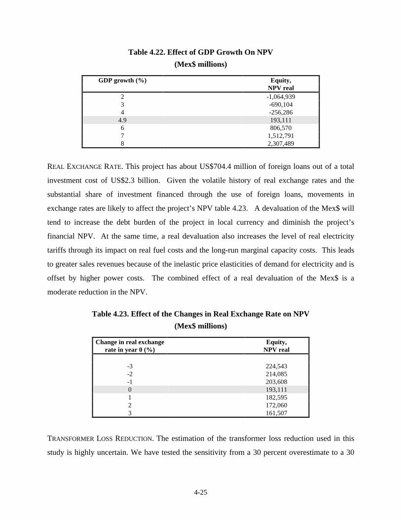
GROSS DOMESTIC PRODUCT (GDP) GROWTH. For the last two decades, demand for electricity has
been growing at some 6 to 7 percent per year. The forecasting models used in this study are
based on income and price elasticities, which project growth in demand of 5 to 6 percent per
year. The rest of the historical growth is explained by other factors such as population growth
and new connections, which are captured by the constant terms used in the equations of the
forecasting model. By changing the growth of income (GDP) in the model, we vary the growth of
demand. We find that the project’s NPV is highly sensitive to GDP growth (table 4.22).
4-25
Table 4.22. Effect of GDP Growth On NPV
(Mex$ millions)
GDP growth (%) Equity, NPV real
2 -1,064,939 3 -690,104 4 -256,286
4.9 193,111 6 806,570 7 1,512,791 8 2,307,489
REAL EXCHANGE RATE. This project has about US$704.4 million of foreign loans out of a total
investment cost of US$2.3 billion. Given the volatile history of real exchange rates and the
substantial share of investment financed through the use of foreign loans, movements in
exchange rates are likely to affect the project’s NPV table 4.23. A devaluation of the Mex$ will
tend to increase the debt burden of the project in local currency and diminish the project’s
financial NPV. At the same time, a real devaluation also increases the level of real electricity
tariffs through its impact on real fuel costs and the long-run marginal capacity costs. This leads
to greater sales revenues because of the inelastic price elasticities of demand for electricity and is
offset by higher power costs. The combined effect of a real devaluation of the Mex$ is a
moderate reduction in the NPV.
Table 4.23. Effect of the Changes in Real Exchange Rate on NPV
(Mex$ millions)
Change in real exchange rate in year 0 (%)
Equity, NPV real
-3 224,543 -2 214,085 -1 203,608 0 193,111 1 182,595 2 172,060 3 161,507
TRANSFORMER LOSS REDUCTION. The estimation of the transformer loss reduction used in this
study is highly uncertain. We have tested the sensitivity from a 30 percent overestimate to a 30

4-26
percent underestimate of the losses in the base case analysis. Table 4.24 summarizes the results.
The transformer loss has only a moderate effect on the project’s NPV.
Table 4.24. Effect of the Transformer Loss Reduction on NPV
(Mex$ millions)
Changes as a percentage Equity, of base case losses NPV real
-30 46,781 -20 95,557 -10 144,334 0 193,111
10 241,888 20 290,664 30 339,441
Economic Analysis
We conducted the economic analysis of the CFE electricity distribution project at the domestic
price level to allow us to analyze the project’s externalities (for more discussion see Harberger
and Jenkins 2001). We estimate these externalities by taking the difference between the
economic net benefit statement and the financial net benefit statement. The first step in
conducting an economic analysis is to determine the economic value of electricity, the economic
costs of foreign exchange and capital, and the economic conversion factors for all inputs used in
the project. We then use these conversion factors to convert the financial statement of net
benefits into the economic statement. Finally, we distribute the externalities among different
stakeholders in the stakeholder analysis.
The Economic Value of Electricity
The measurement of the economic value of the output of a project differs markedly between a
competitive industry and a regulated industry. A few countries have deregulated and introduced
competition in their power industries; however, in most countries where the power industry
remains regulated, a power project is typically the investment of a regulated power company

4-27
within a regulated industry. The following discussion assumes that the power company
concerned is such a regulated utility.
ECONOMIC VALUE OF ELECTRICITY IN A COMPETITIVE INDUSTRY. In a competitive market, when a
project increases the industry’s supply of electricity (supply curve AS shifts to AS’ in figure 4.1),
the price of electricity falls, quantity of electricity demanded rises, and the production of existing
producers decreases. The increase in consumer welfare or willingness to pay is equal to the area
HEFG. The resources released by the reduced production by existing firms is given by the area
IJEH. The economic value of the project’s output is the sum of these two areas.
Figure 4.1. The Impact of a New Project in a Competitive Industry
In the case of a regulated electric utility, the increase in supply from one of its new
projects does not cause the price to change, because the price is regulated. A regulated utility
typically increases its supply to meet a potential power shortage situation at a given price. The
value of the electricity supplied by a regulated utility is considered later.
VALUE OF ELECTRICITY WITH POWER SHORTAGES. When a power shortage situation arises and
persists for some time, some firms and residential customers may decide to install their own
generators, others may decide to manage without electricity, while still others may simply cut
back on some of their activities that require electricity. Furthermore, some firms that otherwise
0
A
B
C
D
E
F
GHI
S
S’
IJEH = Saving in resources due to the production cut back of existing firms
J
Price
Quantity
Demand

4-28
would have located in the country or state may decide not to. We shall refer to the potential
demand for electricity discouraged by power shortages as deterred demand.
A power project that provides electricity to customers during power shortages or to
customers without a connection to the power supply will have a direct impact on the consumers
affected by the power shortages and an indirect impact on the economy by eliminating the
deterrence to potential domestic and foreign investment in the state.
The direct benefits of providing electricity are measured by customers’ willingness to pay
for power. In addition to the direct benefits accruing as a result of the elimination of power
shortages, additional benefits arise from the reduction in deterred demand. Because of the lack
of a good measure of the quantity of deterred demand, these benefits are not included in this
study, but they are nevertheless an important consideration.
In figure 4.2 the supply of power by the existing system is fixed at the level Q0 in year 0,
represented by the vertical supply curve, Q0S0. Based on the demand curve DD0, the demand for
power would have been Q1 at the prevailing tariff of P0 at year 0, but because of the fixed supply
at Q0, a power shortage of AE persists. The valuation of electricity currently provided is given
by the area 0DFA. The valuation of the entire demand (served and unserved), Q1, is given by the
area 0DCE. If the power shortage is evenly distributed among all customers through a rotating
blackout, the valuation of the unserved energy or shortage power is given by the area AFDCE.
After the deterred demand is added, the new demand curve is represented by the line DC’D’.

4-29
Figure 4.2. Demand and Valuation of Electricity with Rotation of Power Shortages
0
P0
P’ D
F
A
C
E E’D0
D’
C’
S0
Q0
B
Q1 Quantity
Price
We can estimate the highest value a customer is willing to pay by the cost of the
alternative power supply available to this customer, which usually means own-generation with a
small gasoline or diesel electricity generator. For a rural farmer the fuel cost of running a diesel
water pump may provide an estimate of the highest level of willingness to pay. For rural
residential usage the cost of using a kerosene stove may be used (see, for example, World Bank
1996).
For own-generated power to have the same degree of reliability as the power obtained
from the electric utility, the own-generation will have to be backed up by another generator. The
maximum willingness to pay for the shortage energy (P’) with “similar to the utility” reliability
can thus be estimated by the cost of own-generation plus the cost of maintaining a reserve
generator. Assuming the capacity cost (cost of generator) takes up k percent of the total self-
generation cost, the maximum willingness to pay will be (1 + k) times the own-generation cost
with no backup.
Let the quantity of the shortage energy (AE) be S (kWhs), the gross of tax price of
electricity (0P0 or AF) be P0 in year 0, and the cost of own-generation or alternative supply be G0.
The highest willingness to pay (WTP) for shortage power is therefore

4-30
maximum WTP = P’ = 0D = (1+k)*G0 (4.3)
We have
area 0DFA = (Pt+(1+k)*G0)*Q0/2 and (4.4) area 0DCE = (Pt+(1+k)*G0)*(Q0+S)/2 . (4.5)
The valuation of the “unserved energy” is given by the area
AFDCE = 0DCE – 0DFA = S*(Pt+(1+k)*G0)/2. (4.6)
Equation (4.6) can be rewritten as
WTPS*S= S*(Pt+(1+k)*G0)/2, (4.7)
where WTPS is the average willingness to pay per unit of shortage power, S is the quantity of
shortage power, and Pt is the prevailing gross of tax price of electricity in year t.
From equation (4.7), the average willingness to pay per unit of shortage power is given by
average WTP = WTPS = (Pt+(1+k)*G0)/2 , (4.8)
that is, the maximum willingness to pay plus the prevailing tariff in year t divided by 2, or
average WTP = (Pt+P’)/2 . (4.9)
For this study, the calculation of the average willingness to pay is given in table 4.25.

4-31
Table 4.25. Own-Generation Costs, Average Tariff, and Willingness to Pay
(1990 prices)
Category Amount Own-generation cost (US$/kWh) 0.210 Average power price in mexico (gross of tax, Mex$/MWH) 0.114 Average power price in mexico (gross of tax, US$/kWh) 0.037 k (capacity cost as a share of total own-generation cost) 0.403 Maximum willingness to pay (US$/kWh) 0.294 Maximum willingness to pay (Mex$/MWH) 0.904 Average willingness to pay (US$/kWh) 0.166 Average willingness to pay (Mex$/MWH) 0.509
MWH Megawatt hour kWh Kilowatt hour
Note that changes in electricity tariffs over time will not affect the maximum willingness
to pay. For this study we assume that the maximum real willingness to pay stays constant in real
terms at its year 0 (1990) level. We calculate the average willingness to pay for each year of the
project as the average of the maximum willingness to pay and the prevailing real tariff.
DETERRED DEMAND. If a region’s power shortages persist, some potential businesses, investors,
and even residents will be discouraged from settling in the region. We refer to this portion of the
potential demand for electricity as the deterred demand. As long as the assumption that the
deterred customers are similar to the existing customers holds, the willingness to pay for the
deterred demand can be represented by the area ECDC’E’ in figure 4.2. We can use equation
(4.9) to calculate the economic benefits per kWh when the deterred demand is considered in the
study.
VALUE OF A BALANCED SUPPLY OF ELECTRICITY. With a balanced power supply there will be no
deterred demand. In figure 4.3 the utility expected the growth in potential electricity demand
caused by population and income growth, represented by the shift of the demand curve D0D0 to
D’D’. The new power project is intended to meet this potential demand. The initial supply of
power, represented by Q0S0, will be shifted to Q’S’. The value of the additional power supplied
by the project is thus represented by the area AFD0D’CE.

4-32
Figure 4.3. Demand and Valuation of Electricity with a Balanced Power Supply
Price
s0
Q0
P0
D’
Quantity
D0
D’
D0
Q’
S’
A
B
C
E
F
0
If the difference between the maximum willingness to pay 0D’ and 0D0 is small and
negligible, we can use equations (4.8) and (4.9) to calculate the total willingness to pay for the
newly supplied electricity9.
The foregoing discussion is based on the assumption that the new power supply does not
affect power prices and that the demand curve for power shifts to the right over time. This
situation often arises with a regulated electric utility that supplies to a captive market. In a
competitive power market, however, a new power project by a competitive supplier may cause
the power supply price to fall. This may lead existing suppliers to reduce production and the
demand for power to rise. In such a case the weighted average of the supply price and demand
price for electricity should be used to value the electricity (Harberger and Jenkins, 2001).
NONTECHNICAL LOSSES: PILFERED ELECTRICITY. Some electricity will always be pilfered from
any power system. We shall refer to the portion of demand that should be metered, but is not, as
pilfered demand or pilfered electricity. For pilfered electricity consumers are likely to consume
the electricity until the marginal utility for their electricity consumption becomes zero. The
willingness to pay for the electricity consumed by these consumers is given by the entire
triangular area under the demand curve in figure 4.4, where P1 is the price of electricity, Q0 is
9 The new maximum willingness to pay 0D’ will be greater than the initial maximum willingness to pay 0D0 if the costs of alternative own generation is higher for those who are deterred from entering the region.

4-33
demand before metered demand equals pilfered demand, and Q1 is demand after metered demand
equals retained pilfered demand.
When meters are installed, these consumers will behave like any other electric
consumers. Two things will happen. First, these newly metered consumers will continue to
consume electricity, but only to the point where the power price is equal to the marginal
willingness to pay. To the utility, this will mean new paying customers and increased sales at no
added costs, except for the meters and metering costs. Assuming that the pilferage behavior is
evenly distributed among all groups of consumers, the reasoning and the estimation of the
economic value of electricity for this portion of electricity demand is identical to the shortage
case. As the consumers were already consuming this portion of pilfered electricity prior to the
installation of new meters, this portion of “retained” pilfered electricity consumption adds no
economic benefits to the consumers. What has occurred is the transfer of monetary payment
from the consumers to the utility.
Figure 4.4. Pilfered Electricity, New Meter Installation, and Curtailed Demand
P1
P’
$
QuantityQ0Q1
0
Willingness to payfor curtailed pilfereddemand
Willingness to payfor retained pilfereddemand
Second, because the newly metered customers must now pay for the electricity they
consume, they will no longer consume the portion of electricity that they previously consumed
but valued at less than the price. The newly metered consumers will lose the value of this portion
of power previously available to them at no cost. The average value or willingness to pay for this

4-34
“curtailed” pilfered electricity, assuming a straight-line demand curve that intersects the
horizontal axis, is equal to one half the electricity tariff now charged.
When new meters are installed for those electricity consumers previously unmetered, the
quantity of the retained demand or consumption is estimated as the number of new meters
installed times the average consumption per customer (Q1 in figure 4.4). We shall assume the
second portion or the curtailed portion of the pilfered electricity to be a percent of the retained
consumption (the first portion of the pilfered electricity, Q1)10. The total willingness to pay for
the curtailed portion of the pilfered demand (WTPCPD ) should therefore be
WTPCPD = AQ1(0.5P1) = 0.5AP1Q1 (4.10)
where P1 is the price of electricity.
As the utility no longer has to generate the curtailed portion of the previously pilfered
demand, it will realize fuel and capacity savings.
TECHNICAL LOSS: TRANSFORMER LOSSES. The new project will reduce previous power losses
caused by transformer overload. After the project the power company is no longer required to
generate the power previously lost. This will result in savings in fuel and generation capacity to
the utility. A financial gain accrues to the utility equal to the marginal generation cost times the
reduction in power losses.
Transformer losses are of two main types: iron loss and copper loss. At a given level of
voltage the iron loss is constant while the copper loss is a function of the square of the current.
An overloaded transformer means that more current is passing through it, and therefore more
copper is lost. One can reduce the transformer losses in overloaded substations by installing new
transformers. By doing so the reduced loads of transformers decrease the copper loss, while the
iron loss remains constant. As the iron loss remains constant, the incremental benefits come only
from reducing the copper loss.
10 Let Q0 be the quantity of electricity pilfered before the project and let Q1 be the quantity of electricity consumed and paid for by the consumers who previously pilfered electricity. Let P’ and P1 be the maximum willingness to pay and the tariff respectively. Assuming a linear demand curve, the following equation holds: A=P1/( P’ - P1 ) = 24.04 percent where P’= Mex$0.652 million/Mwh and P1 =Mex$0.126 million/Mwh in 1990.

4-35
To evaluate the loss we calculate the overall running cost of the transformers before and
after the project. The overall annual running cost of a transformer equals the annualized capital
cost plus the fuel cost. The annual cost of power loss is given by the following:
annual cost of iron loss = LI *( C+ 8760 * FC ) and (4.11)
annual cost of copper loss = LC * D2 *( C+ 8760 * FC *DLF* TLF) (4.12)
where LI is the iron loss in the system in kilowatts (kW); LC is the copper loss in system in kW;
C is the annual charge per kW of maximum demand; FC is the fuel cost (Ps/kWh), D is the
demand factor which is equal to maximum demand/full-load rating of transformer; capacity; TLF
is the transformer load factor; and DLF is the demand load factor.
The incremental annual cost of iron loss is zero, because the iron loss, the fuel cost, and
the capital charge per kW are constant with or without the project. The incremental annual cost
of copper loss varies with the square of the demand factor.
As of 1988, 29 percent of the substations were operating at 118 percent of their nominal
capacity. This project aimed at reducing this load to 98 percent by 1994. Without this project
CFE estimated the loss to be 623.38 MW in 1994. If we assume that the transformers have a
ratio of copper loss to iron loss of four to one, the copper loss is therefore 498.7 MW (0.8 *
623.38 MW). The copper loss with the distribution project in 1994 can therefore be calculated as
follows;
new copper loss = 498.7*[(.98/1.18)^2].
The annual reduction in energy loss will be given by
reduction in energy loss = (old copper loss – new copper loss) * 8760 * load factor. (4.13)
The reduction in energy loss means that CFE will be able to supply the same electricity
demand with less power generation and transmission. This means a savings in fuel and capacity
costs for the utility.

4-36
The Economic Costs of Capital and Foreign Exchange
We estimated the real economic cost of capital for Mexico to be 12.3 percent. This cost was
determined as a weighted average of the different domestic net-of-tax saving rates, the gross-of-
tax returns on investment for the different sectors, and the marginal costs of foreign borrowing.
We found the economic cost of foreign exchange to be 10.61 percent higher than the
official exchange rate. This premium is due partly to the impact of net import tariffs and value
added taxes. We also assume that the current account deficit will be sustainable.
Conversion Factors for Inputs
BASIC CONVERSION FACTORS. Investment and operating costs components consist of individual
items such as: freight, insurance, nontradable and tradable materials and equipment, and tradable
fuel costs. Before calculating the conversion factors for the investment and operating items, we
have to determine the basic conversion factors of the above individual items.
We made the following assumptions for import tariffs, local freight and insurance costs,
and nontradable materials:
• Import tariff: The import tariff used in this study is 10 percent. This rate is admissible
given the prevailing rates applicable after the March 1989 trade regime11.
• Local freight and handling. We also estimated the local freight and insurance costs to be
10 percent of the cost, insurance, and freight value. We assumed the supply and demand
weights for freight and handling to be 80 and 20 percent respectively. We also considered
that freight and handling were 50 percent tradable.
• Nontradable materials. We assumed a 50 percent weights for supply and a 50 percent
weight for demand, and a 20 percent content of tradable components. We assumed that
the proportions of the quantity of nontradables purchased by the project that are
accommodated by increased supply and decreased demand are 50 percent for each. The
foreign exchange content of the nontradable materials is assumed to be 20 percent.

4-37
Using these assumptions we calculated the basic conversion factors, adjusted by the
foreign exchange premium, for freight and handling, tradable materials and equipment,
nontradable materials, and tradable fuel.
INVESTMENT COST ITEMS. For each component of the distribution subprogram we broke down the
investment cost into tradable and nontradable materials and skilled and unskilled labor. We then
calculated the conversion factors for tradable and nontradable materials. The conversion factors
for labor came from an Inter-American Development Bank study (1998). Finally, we estimated
the conversion factor for each investment line as the weighted average of the conversion factors
of its components. For instance, the cost of primary feeders is made up of 68 percent of tradable
materials, 15 percent of nontradable materials, 11 percent of skilled labor, and 6 percent of
unskilled labor. Given these respective cost shares and the respective 0.999, 0.944, 0.734, and
0.482 conversion factors for tradable materials, nontradable materials, skilled labor, and
unskilled labor, we calculate the conversion factor for the primary feeders to be 0.931. Tradable
materials and equipment are also adjusted for the foreign exchange premium.
OPERATING COST ITEMS. The operating costs in this study consist of such items as wages,
maintenance and repair materials, but exclude generating costs such as fuel costs. The
conversion factor for operations and maintenance is the weighted average of the conversion
factors for labor and material as estimated for maintenance.
GENERATION COST ITEMS. Generation costs consist mainly of fuel and capacity costs. The
conversion factor for generation of 1.094 is calculated based on shares and conversion factors
shown in table 4.26.
11 Mexico Tax Reform for Efficient Growth, World Bank Report No 8097-ME, pg 78

4-38
Table 4.26. Shares and Conversion Factors of Generation Cost Components
Cost item Share Conversion factor
Fuel 0.5 1.253
Material (tradable, equipment) 0.3 0.999
Material (nontradable, civil works) 0.1 0.944
Skilled labor 0.1 0.734
Generation 1.094
Results of the Economic Analysis
We applied the conversion factors to the real cash flow from the total investment point of view to
obtain the economic cash flow statement (table 4.27). The overall economic NPV of the
distribution project is Mex$239 billion or US$78 million. The project is economically justifiable
because it earns more than the 12.3 percent real economic cost of capital in Mexico.

4-39
Table 4.27. Economic Cash Flow Statement, Selected years 1990-2015
(Real 1990 prices)
Category NPV 1990 1991 1992 1993 1994 1995 1996 1997 1998 2014 2015RECEIPTSREVENUE 3
New connection salesa 3460275 82778 180737 279855 378734 482686 510362 526330 522334 521647 539243 Retained pilfered demand 0.000 0 0 0 0 0 0 0 0 0 0 0 Consumers loss from curtailed pilfered demand -132591 -1716 -4243 -7425 -11331 -16376 -19560 -22686 -22507 -22472 -23091 Savings due to curtailed pilfered demand 1.094 312171 9151 19396 29039 37825 46006 46103 44712 44361 44290 45510 Savings from transformer loss reduction 1.094 364837 30492 34390 38494 43439 49381 48833 48291 47755 47225 39504 Reliability improvement 3.071 211022 2045 5090 9890 16734 25689 26430 27211 28447 29902 69940 Change in accounts receivable 1.000 -115760 -6578 -10555 -14373 -18814 -25258 -20547 -21969 -10795 -11264 -12096 78933 Government contributions 0.000 0 0 0 0 0 0 Consumer contributions 0.000 0 0 0 0 0 0Total net revenue 4099953 116173 224816 335479 446589 562128 591621 601889 609595 609329 659012 78933LIQUIDATION INCOME Building 1.000 0 0 0 0 0 0 0 0 0 0 8499 Vehicles 1.000 0 0 0 0 0 0 0 0 0 0 0Total liquidation income 0 0 0 0 0 0 0 0 0 0 8499Cash Inflow 116173 224816 335479 446589 562128 591621 601889 609595 609329 659012 87432
EXPENDITURESInvestment costs Substation improvements 0.933 146037 157786 139170 123224 68586 Subtransmission lines 0.931 41521 55250 41691 34513 34690 Primary feeders 0.931 5528 8087 11653 15719 18916 Supervisory control equipment 0.950 4129 5930 8490 11459 13828 Distribution lines 0.931 11065 37560 68975 107437 135432 Capacitors 0.999 13825 19888 28368 38274 45940 Reclosing equipment 0.999 30470 44358 63272 85238 102535 Secondary network improvement 0.915 25718 87430 159987 247715 310675 Voltage regulators 0.955 1650 2322 3387 4289 5228 Vehicles and equipment 0.999 120155 102994 117188 135385 137584 Metering equipment 0.973 76445 110904 157935 212092 254340 Computer equipment 0.986 7356 10320 14495 19693 23343 Other equipmemts 0.999 5875 8508 12091 16204 19390 Buildings 0.905 9927 26948 52630 83977 112792 Maintenance 0.661 53257 63712 68256 67518 67578 Rural electrification 0.932 35824 41589 48292 56089 60614Cost overruns 0.879 0 0 0 0 0 Total investment 588782 783587 995880 1258825 1411475Operating expenses for metering of previously pilfered electricity*0.661 78 194 339 518 748 894 1037 1029 1027 1055 0Added generation costs for reliability improvement 1.094 0 0 0 0 0 0 0 0 0 0Working capitalChange in accounts payable 1.000 -16594 -20825 -22281 -23144 -24265 -11300 -8631 -10173 -10619 -11521 74897Change in cash balance 1.000 16594 20825 22281 23144 24265 11300 8631 10173 10619 11521 -74897Total change in working capital 0 0 0 0 0 0 0 0 0 0 0Bad debt 0 0 0 0 0 0 0 0 0 0 0 0TaxesSales taxes 0Income tax 0Cash outflow 3,860,276 588860 783781 996219 1259343 1412223 894 1037 1029 1027 1055 0Environmental impact 435 50 50 50 50 50 50 50 50 50 50 50NET CASH FLOW 239,713 -472737 -559015 -660790 -812805 -850145 590677 600803 608516 608252 657906 87382
NPV economic discount rate (real Mex$ billions) 12.3% 240NPV (real in US$ billion) 78.06 In Mex$ billion (for risk simulation) 239.7Internal Rate of Return (IRR) 13%

4-40
Sensitivity Analysis of the Economic Analysis
The economic NPV is affected by similar variables to those that affect the financial NPV.
However, because the economic values of different revenue and cost items are measured
differently from their financial prices, the resulting economic NPV will differ substantially from
the financial NPV. In the economic sensitivity analysis we shall look at how various variables
affect the economic NPV.
We conducted a sensitivity analysis to identify the key variables and to assess their
impact on the project’s economic NPV. We identified six key variables, which are discussed in
the following paragraphs.
COST OVERRUNS. As table 4.28 shows, the project’s economic NPV is sensitive to investment
cost overruns.
Table 4.28. Effect of Cost Overruns on NPV
(Mex$ millions)
Cost overrun Economic factor (%) NPV real
-20 972,917 -10 606,315 0 239,713 5 56,411
10 -126,890 15 -310,191
INFLATION. Items such as cash balance, accounts receivable, accounts payable, and electric tariffs
will be affected by inflation, and will in turn affect the economic NPV. Even though the
economic NPV increases with greater inflation12, the overall impact of inflation on economic
NPV is small in this project. Table 4.29 summarizes the effect of inflation on the economic NPV.
12 Inflation affects the economic NPV because of its impacts on the real amount of cash balances, accounts receivable, and accounts payable. Also, because of the impact of indexing lag, a higher inflation rate reduces real electric tariffs, which lower the average willingness to pay but increase the quantity of electricity demanded. The combined effects of these factors on economic NPV is uncertain.

4-41
Table 4.29. Effect of Inflation on NPV
(Mex$ millions)
Inflation Economic rates NPV real
5 229,908
10 234,367 15 239,713 20 245,080 25 250,218
FUEL COSTS. Higher fuel costs will increase the savings from the transformer loss reduction, and
hence improve the economic NPV. However, higher fuel costs also mean higher tariffs that
depress demand. A smaller demand means smaller benefits for newly connected customers.
These two effects tend to offset each other, leaving a moderate negative impact on the economic
NPV (table 4.30).
Table 4.30. Effect of Fuel Costs on NPV
(Mex$ millions)
Percentage increase in Economic real fuel cost NPV real
-15 389,617 -10 338,919 -5 288,962 0 239,713 5 191,139
10 143,213 15 95,907
GDP GROWTH. Higher GDP growth will increase the demand for electricity and the per customer
consumption of electricity which in turn will affect the economic benefits to the newly connected
customers as well as the gain from reliability improvement. The results given in table 4.31 show
that changes in the growth rate of GDP, which translate into changes in demand for electricity,
have a significant impact on the economic NPV.

4-42
Table 4.31. Effect of GDP Growth On the growth of Electricity Demand on NPV
(Mex$ millions)
GDP growth (%) Economic NPV real
2 -652,575 3 -380,055 4 -72,169
4.9 239,713 6 655,911 7 1,123,905 8 1,639,007
REAL EXCHANGE RATE. An increase in the real exchange rate will also increase the peso cost of
tradable investment items. This effect will reduce the economic NPV. However, as the fuel costs
are linked to the exchange rate, an increase in the real exchange rate will raise the fuel costs, and
hence the savings from the reduced power generation caused by the loss reduction and curtailed
pilfered consumption. Moreover, as electricity prices are allowed to adjust to the cost of fuel, an
increase in the real exchange rate will also raise the electricity tariffs, reducing the quantity of
electricity demanded. The higher tariffs will increase the average economic value per unit of
electricity consumed by the newly connected customers. Thus the net impact of the real exchange
rate is uncertain. In this study a devaluation has a moderate negative impact on the economic
NPV (table 4.32).
Table 4.32. Effect of a once and Final Real Exchange Rate Change on NPV
(Mex$ millions)
Real Exchange Economic Rate Change (%) NPV real
-3 351,386 -2 314,122 -1 276,898 -0 239,713 1 202,566 2 165,457 3 128,386
ALTERNATIVE POWER SUPPLY COST. The per kWh economic value of electricity supplied to
newly connected customers depends on the estimate of the cost of an alternative power supply,

4-43
which is defined as a multiple (n) of the benchmark electric tariff of 1990. For this study we
estimate that the cost of own-generation is 5.04 times the average gross-of-tax electric tariff in
Mexico in 1990, or Mex$904 per kWh. As table 4.33 shows, the economic NPV is extremely
sensitive to the alternative power supply cost factor.
Table 4.33. Effect of an alternative Power Supply Cost Factor on NPV
(Mex$ millions)
Alternative Supply Economic Cost Factor NPV real
-25 -662,847 -15 -307,792 -10 -126,895 -5 55,704 0 239,713 5 424,901
10 611,088 25 1,174,307
Stakeholder Analysis
In the case of a regulated electric utility, the increase in supply from a new project does not cause
the price to change. A utility typically increases its supply to meet a power shortage situation at a
given price. With the additional output from the project, the utility’s existing output and output
price are not affected. In figure 4.5, when the product price is 0B, the initial production is 0H.
The potential demand is 0G. There is a supply (power) shortage of HG. The initial consumer
surplus is BDF. When the project increases total output by HG, the consumer surplus gain
(FDC) is equal to the economic value of the project output or shortage power (HFDCG) less the
financial value of the output (HFCG ).13 We compute this consumer surplus gain as the
externality that is the difference between the economic value of the electricity and the gross of
tax sales revenue from the sale of the same electricity.
13 Because CFE operates in a regulated environment, the distributional impact of electricity consumption is calculated somewhat differently than the standard procedure explained in Harberger and Jenkins (2001). The basic concept remains the same.

4-44
Figure 4.5. The Impact of a New Project in a Regulated Industry
D
B
D0(Unrationed demand)
CF
GH0
S’= S0 + projectS0(initial supply)Rationed demand’s willingness to pay
Quantity
Price
Measurement of the Impact of Project Cost on Stakeholders
The externality of generation cost savings due to transformer loss reduction and the curtailment
of part of the pilfered demand is distributed between a government revenue gain and a labor loss
for the following reasons. As we can see from table 4.34, the main cause of the divergence
between the economic and financial values of fuel is due to the premium on foreign exchange
and the 25 percent government subsidy on the fuel price. As the utility no longer has to generate
the lost power, it will not have to purchase the fuel for this power, thus the government gains
from not having to provide the fuel price subsidy and from the foreign exchange premium saved.
This explains why we allocated the fuel cost externality mainly to the government.

4-45
Table 4.34. Fuel Cost Conversion Factor
Item Financial
value Conversion
factor
Economic value unadjusted for
foreign exchange premium
Percentage
tradable
Foreign exchange premium
(%)
Financial value *
percentage tradable *
foreign exchange premium
Economic value
adjusted
Free on board price 1,000 1 1000 100 10.61 106.12 1106.12 Port charges,
transport and insurance 100 0.933 93.3
Local freight and handling 90.00 0.933 83.93
Sales tax 134.88 Subsidy 250 Total 875 1096.75 Conversion factor 1.253
Another example is the allocation of the generation cost externality. As table 4.35 shows,
the major divergences between the economic and financial costs of the inputs occur in the fuel
and skilled labor costs. For this reason, the externality of the generation cost was allocated
between the government and labor.
Table 4.35. Generation Cost Conversion Factor Calculation
Item Share (%) Conversion factor Fuel 0.5 1.253 Material (tradable, equipment) 0.3 0.999 Material (nontradable, civil works) 0.1 0.944 Skilled labor 0.1 0.734 Conversion factor 1.094

4-46
Allocation of Project Externalities: Overall Results
Table 4.36. Distribution of Project Externalities.
(1990 Prices)
Stakeholder (Mex$ millions) (US$ millions) Government 725,063 236 Consumers Newly connected 2,489,321 811 Payment for previously pilfered electricity -1,831,753 -596 Curtailed pilfered demand -131,989 -43 Previously affected by power failures 182,358 59 Labor 96,694 31 Society -432 -0.1
CONSUMERS. Consumers will have the most to gain from this project, but the impacts on the
different types of consumers are quite different.
The connections to new customers are a major economic gain for the economy. Without
new connections this group of new customers would either have to do without electricity or to
generate their own electricity. The cost of alternative power generation is typically two to three
times the utility’s marginal power generation cost. This high alternative power generation cost
also means a high willingness to pay for power by those customers who would have to live
without it if the new connections were not made. This has led to a high consumer surplus gain of
Mex$2,489 billion in real NPV to the newly connected consumers.
While the newly connected customers are the biggest winners in terms of economic
benefits, the newly metered customers who had hitherto been unmetered are big losers
financially, as they now have to pay for the electricity they were able to consume for free before.
In addition to these financial losses, this group of customers will also reduce its power
consumption to the point where their willingness to pay is equal to the electric tariff. Those
customers who had previously pilfered electricity will continue to consume the major portion of
their previous consumption, but will lose a small portion whose value is now less than the price
of the electricity. While these consumers will not gain or lose in utility on the first portion of
their consumption, they will lose financially in having to pay for the power for which they did not
have to pay before. This financial loss amounts to Mex$1,832 billion. The curtailment of part of

4-47
the previously pilfered electricity represents a consumer surplus loss of Mex$132 billion to this
group of consumers. The total loss suffered by this group of customers is thus Mex$ 1,964
billion.
The improvement of power reliability is another source of economic gain. The cost of
power failures to consumers is high, 12.5 times the 1990 electric tariff. Gutierrez (1991, p. 8)
estimated it to be US$1 per kWh versus the long-run marginal power cost of US$0.07 per kWh.
Electricity consumers’ willingness to pay for electricity during power failures is therefore high.
Even though the reduction in power failure time is only 136 minutes per year, it adds Mex$182
billion of consumer surplus to CFE’s customers.
Overall, consumers as a whole will gain Mex$705 billion from this project.
LABOR. The labor sector has a gain of Mex$97 billion, mainly from its participation in the
construction of the investment projects and employment in the production of power. This gain is
due partly to the protected sector wages being higher than the opportunity cost of labor. When
the utility reduces power production because of the reduction in transformer loss, the labor sector
will lose some financial benefits. When the utility increases power production, labor will gain
some financial benefits.
THE GOVERNMENT. The government gains significantly from the sales tax it collects from
electricity sales to newly connected and newly metered customers. This gain is somewhat offset
by the increase in the government’s oil price subsidies. The government will also gain from the
import duties it will collect on the materials, machinery, and equipment that are to be imported.
Offsetting this revenue gain is the loss the government incurs through the foreign exchange
premium that is lost when the project uses tradable goods inputs. Overall the government will
gain Mex$725 billion from the project.
Poverty Alleviation
Electricity projects can have both a direct and an indirect impact on poverty alleviation.

4-48
DIRECT IMPACT. The economic welfare of a group of people can be measured by the aggregate
monetary income of the group or by the economic welfare the group enjoys. Governments often
find it necessary to provide their poorer citizens with essential services such as transportation,
water supply, electricity, health care, and schools. These services are often labeled as
necessities. In the framework of a cash flow analysis, they simply mean services that command a
high willingness to pay when they are not available. When the government provides roads and
schools free of charge, the citizens who benefit are receiving a high consumer surplus that is
equal to the willingness to pay less monetary charges, which in this case are zero. If this group of
consumer-surplus recipients also belongs to the low-income group, the gain of the consumer
surplus by this group is a measurement of poverty alleviation, even if the consumer surplus is not
provided in any monetary form.14 When a project directly provides a product or service such as
electricity to the low-income group, the poverty alleviation impact of the project can be measured
by the consumer surplus gain by this group of electricity customers. This is what we shall call
the direct poverty alleviation impact of a project.
In this study the share of the low-income group in total residential customers is 40
percent, and we assume that, on average, the group’s maximum willingness to pay is 80 percent
of the maximum willingness to pay of all customers. We can calculate the direct poverty
alleviation impact as follows.
direct impact = (quantity of electricity sales to new residential customers)*
(low-income group share)* {(maximum WTP+tariff)/2 – tariff} (4.14)
We estimate the direct poverty alleviation impact of this project at Mex$294 billion.
INDIRECT IMPACT. Other than the direct poverty alleviation impact provided by the direct
consumption of a project’s output by the low-income group, a project can also be beneficial to
the economy, which in turn will benefit the low-income group indirectly through higher
employment and better wages. We shall call this the indirect poverty alleviation impact of the
14 Note that the willingness to pay measurement is actually a measurement of the monetary equivalent of the goods or services that the group receives.

4-49
project and do not calculate it in this study. In principle, this indirect impact can be measured by
an accounting of the employment and wage impacts on the low-income group.15
ENVIRONMENTAL IMPACT. There is a small negative environmental impact of Mex$432 million
that is borne by society at large. The environmental impact of distribution is small, because it
involves only small substations, transformers, and low-voltage wires. Occasionally unsightly
wires may also have a negative impact.
RECONCILIATION OF ECONOMIC, FINANCIAL AND DISTRIBUTION ANALYSIS. Using a common real
economic discount rate of 12.3 percent, we find that the values in this case reconcile so that the
economic NPV is equal to the financial NPV (evaluated using the economic discount rate) plus
the sum of the distributional impacts brought about by the project (table 4.37).
Table 4.37. Reconciliation of Economic and Financial Values of Inputs and Outputs
(Mex$ millions, real)
Economic NPV at economic discount rate
= Financial NPV at economic discount rate
+ Present value of externalities at economic discount rate
239,713 = -1,252,322 + 1,492,034
Risk Analysis of Financial and Economic Returns
The base case analysis provides a single-value scenario with assumptions reflecting their most
likely values. It does not provide a full picture of the project risk. To overcome this deficiency we
conducted a risk analysis that takes into account the variability of those variables identified in the
sensitivity analysis. Table 4.38 shows the probability distributions of the assumptions.
The risk variables in this project are the inflation rate, the investment cost overrun factor,
the change in real fuel costs, the growth of GDP (which affects growth in demand), the average
level of the real exchange rate, the quantity of transformer loss reduction, and the alternative
15 Wage content of output ={(electricity sales (pesos) to industrial customers) / (electricity input/output ratio) }* (labor input/output ratio). Indirect impact = incremental wage bill that is due to electricity provided by the project. The same formula can be applied to commercial customers.

4-50
power supply cost factor. Note that even though the electric tariff is an important factor in
deciding the financial NPV, we have not included it in the risk analysis because it is a policy
variable.
Table 4.38. Assumptions of Risk Variables
Risk variable Probability distribution Base case mean value (%)
Range value (%)
Probability distribution (%)
Inflation rate
Step (independent yearly) 15 0 to 5 5 to 10
10 to 15 15 to 20 20 to 25 25 to 30 30 to 35
5 15 40 20 10 5 5
Investment cost overrun factor
Normal 0
15 to 15
Mean 0, Standard deviation 4
Annual percentage change in real fuel costs
Step (independent, yearly) 0
-40 to -30 -30 to -20 -20 to -10 -10 to 0 0 to 10
10 to 20 20 to-30 30 to 40
4 13 25 17 8 8
13 13
GDP growth Normal 4.9 1.9 to 7.9
Mean 4.9, Standard deviation 1
Percentage change in average real exchange rate
Normal 0 -23 to 23
Mean 0, Standard deviation 7.75
Transformer loss reduction factor
Normal 0
-15 to 15
Mean 1 Standard deviation 5
Alternative power supply cost factor
Normal 0
-25 to 25 Mean 0 Standard deviation 5
Risk Variables
INFLATION. Inflation in Mexico remained low in the 1960s and until 1972 (figure 4.6). The 1973
oil price hike by the Organization of Petroleum Exporting Countries (OPEC) led to double-digit
inflation in 1973. Subsequently inflation peaked at more than 120 percent around 1988, before
dropping in the early 1990s.

4-51
Figure 4.6. Inflation in Mexico, 1949-96
Mexico Inflation, 1949-1996
-20%
0%
20%
40%
60%
80%
100%
120%
140%
1949
1953
1957
1961
1965
1969
1973
1977
1981
1985
1989
1993
Years
Inf lation
Fiscal discipline, monetary policy, and trade balances are the main determinants of
inflation and exchange rate adjustment in Mexico. The year-to-year changes in inflation and
exchange rate adjustment may be viewed as fluctuations around their general levels subjected to
random influences. Of course, long-term inflation and exchange rate forecasts must be subject to
these uncertainties. One cannot predict the political environment, government policy, and
international forces with precision. To the extent that we can, in general, assume that the
government will learn from experience and that our present understanding of the economy is
sufficient, the range of inflation and exchange rate fluctuations will narrow over time.
The inflation and exchange rate assumptions used in project appraisal are therefore
subject to two risks: (a) the average level risk over the duration of the project, which has a
narrower range of fluctuation and is more stable and predictable; and (b) the annual variation
risk, which has a wider range of fluctuation because of more random factors. With Mexico
adopting stricter monetary and fiscal discipline, we can expect a gradual improvement in the
management and control of inflation. In our cash flow model we use a long-term inflation rate of
15 percent to approximate this prospect and a step distribution to represent the annual
disturbances (table 4.38).

4-52
FOREIGN EXCHANGE RATE. As noted, inflation and exchange rate fluctuations in Mexico are
closely related. Exchange rate fluctuation is determined by the current account balance,
international capital flows, and relative inflation rates in Mexico and the United States. Prior to
1975, the Mexican exchange rate was pegged at Mex$12.5 per US$1. As figure 4.7 shows, a
huge devaluation of 267 percent in 1982 followed nearly a decade of double-digit inflation.
Further large devaluations took place in subsequent years. During 1975-96, annual changes in the
nominal exchange rate had a mean of 46.5 percent per year and a standard deviation of 67.6
percent. After we adjust the nominal exchange rates by the relative inflation (nominal exchange
rates deflated by Mexican Consumer Price Index/United States Consumer Price Index), the
variation in the real exchange rates has a mean of 7.6 percent per year with a 40.4 percent
standard deviation.
Figure 4.7. Real Exchange Rate, Trend, and Deviations from Trend, 1954-96
1954-1996
-0.50
0.00
0.50
1.00
1.50
2.00
2.50
3.00
3.50
4.00
1954
1958
1962
1966
1970
1974
1978
1982
1986
1990
1994
Years
Pes
os/
$ Real Exchange Rate
Deviations from Trend
Trend (Real Exchange Rate)
With austere government budgets and a stringent monetary policy in place, real exchange
rates are likely to be stable in the future, with small, annual, nominal, upward adjustments to
reflect the higher inflation rate in Mexico. In figure 4.7 a trend line is fitted to Mexico’s real
exchange rates that indicates a small upward trend. The errors between the actual and calculated
values have a mean of 0 percent and a standard deviation of 35.5 percent.

4-53
For the purposes of the risk analysis it is the level of the average real exchange rate that
the project experiences over its life that has the most significant impact on the project’s outcome.
Given the high volatility of the year-to-year changes in the real exchange rate, most of these
annual changes cancel each other out. If we take it as given that the annual changes in the real
exchange rate have a mean of 0 and a standard deviation of 35.5 percent, then the movement of
the mean real exchange rate averaged over the life (31 years)of the project will have a mean of 0
and a standard deviation of 7.75 percent. It is this normal distribution that we use in the risk
analysis of the project.
FUEL COSTS. While the market power of the OPEC cartel seems to exert decisive influences on
world oil prices at times, the true long-term forces that determine oil prices are the demand for
and supply of oil and production costs. Figure 4.8 shows the U.S. imported oil price for 1973-97.
Following each price hike, the demand for oil adjusted and the oil price declined and stabilized.
The yearly ups and downs in oil prices are heavily affected by unpredictable, near-random
incidents, such as wars in the Middle-East, OPEC decisions, and the weather.
Figure 4.8. U. S. Nominal Oil prices and Annual changes, 1973-97
Nominal oil price (US$)Nominal annual change (%)
-60-40-20
020406080
100
1973 1976 1979 1982 1985 1988 1991 1994 1997

4-54
Figure 4.9. Real U.S Imported Oil Prices, Trend, and Deviation from Trend, 1973-96
During 1975-97 the changes in the average nominal U.S. import price of crude oil had a
mean growth rate of 9.4 percent and a standard deviation of 28.7 percent. The average
compound growth rate of oil prices during the same period was 3.2 percent. While the nominal
oil prices exhibit a small upward trend of around 3 percent per year, the real oil prices shows no
long-term trend: the average compound growth rate of real oil prices from 1975-96 was –0.23
percent16. Based on this historical background, we have assumed a long-term growth rate of 0
percent for real oil prices. In figure 4.9 we fit a trend line to the real oil price data. Based on the
trend values and the actual values, table 4.39 presents the probability distribution of the errors
used in the study.
16 The mean growth rate of real oil prices is 2.6 percent with a standard deviation of 24.9 percent.
-10
-5
0
5
10
15
20
1973 1975 1977 1979 1981 1983 1985 1987 1989 1991 1993 1995
Real oil price Calculated oil price Deviation from trend
US$/barrel

4-55
Table 4.39. Probability Distribution for Annual Disturbances of Real
Oil Prices Used in the Study (percent)
Error Probability
-40 to -30 4 -30 to -20 13 -20 to -10 25 -10 to 0 17 0 to10 8
10 to 20 8 20 to-30 13 30 to 40 13
Total 100
INVESTMENT COST OVERRUNS. Typically, investment cost estimates include a contingency
provision. These estimates are treated as the expected values of the investment costs. We
assume that actual investment costs will fluctuate around the expected values with a normal
distribution, which has a standard deviation of 4 percent of the investment costs (table 4.38).
DEMAND FOR ELECTRICITY. The demand for electricity is a function of GDP. We used a normal
distribution with a mean of 4.9 percent and a standard deviation of 1 percent to represent the
annual fluctuations around the expected growth of GDP (table 4.38).
TRANSFORMER LOSS REDUCTION. The estimated value of the transformer loss it is uncertain. To
deal with this uncertainty we assumed a normal distribution with a mean of 0 and a standard
deviation of 5 percent (table 4.38).
ALTERNATIVE POWER SUPPLY COST FACTOR. The economic value of shortage power depends on
the estimated cost of an alternative power supply. To incorporate the possible variation in our
estimate of the alternative supply cost we assumed that the alternative power supply cost factor
has a normal distribution with a mean of 0 percent and a standard deviation of 5 Percent (table
4.38).

4-56
Results of the Risk Analysis
The results of the risk analysis summarized in table 4.40 shows that the expected value of the
financial (equity) NPV is Mex$191 billion, which is close to its base case value of Mex$193
billion. The expected economic NPV is Mex$362 billion, which is higher than its base case
value of Mex$239 billion. The difference, however, is small relative to the total cost of the
investment.
Table 4.40. Expected NPV from Risk Analysis
(Mex$ billions, real)
Category Financial NPV - Equity Economic NPV Base case 193 239 Risk analysis Expected value 191 362 Minimum value Maximum value Probability of negative NPV (%) 37 25
While the project’s final outcomes remain uncertain, the risk analysis helps define the scope of
these outcomes. There is a 25 percent chance for a negative economic NPV and a 37 percent
chance for a negative financial NPV. The financial variability of the outcome could threaten the
project’s sustainability if it were operated by the private sector. However, as this project is part of
the activities of a state-owned enterprise, the 37 percent probability of the project creating a
negative financial NPV may not threaten it to the same degree.
Conclusion
The project is both economically and financially feasible, but is somewhat risky in terms of its
financial and economic performance.
The distributive analysis shows that newly connected consumers will receive a large
consumer surplus gain, previously unmetered customers will undergo a large financial loss, and

4-57
the government can expect a large revenue gain. The low-income segment of newly connected
customers will receive a consumer surplus gain of about Mex$294 billion, while the labor sector
will receive a modest gain of Mex$96 billion.
Overall the project is worthwhile, but the control of investment costs, the willingness to
pay, and the growth of GDP are all critical variables determining its economic feasibility.

4-58
REFERENCES
Commission Federal de Electricidad 1989a. “Proyecto especial para la rehabilitation y
modernizacion de unidades generadoras des area de generacion thermoelectrica de CFE, 1989,Programa No.1 Unidades de 300/350 MW”.
1989b. “Programa de inversiones en el area de distribution.” Gutierrez, Luis E. 1991. “Economic Analysis of a Power Investment Program.” World Bank,
Washington, D.C.. Inter-American Development Bank, 1988. Los precios de cuenta en Mexico 1988, 2nd ed.
Mexico City: National Finananciera. Jenkins, Glenn P. 1985. “Public Utility Finance and Economic Waste.” Canadian Journal of
Economics (August). Jenkins, Glenn P., and Mostafa B. El-Hifnawi. 1994. “Economic Parameters for the Appraisal of
Investment Projects: Bangladash, Indonesia, and the Philippines.” Report for the Asian Development Bank, Economics and Development Centers. Manila.
Harberger, A.C. and Jenkins, G. P., 2001. Cost-Benefit Analysis of Investment Decisions.
Kingston, Ontario, Queen’s University. Lim, Henry B. F. 1979. “Cost-Benefit Analysis for Peak-Load Pricing and Load Management.”
Ph.D. dissertation, University of Chicago. Taylor, Lester D. 1975. “The Demand for Electricity: A Survey.” Bell Journal of Economic, 6(1). Westley, Glenn D. 1992. New Directions in Econometric Modelling of Energy Demand.
Baltimore, Maryland: The Johns Hopkins University Press. World Bank. 1990. “Mexico Transmission and Distribution Project.” Staff Appraisal Report no.
8191-ME. Wasnington, D.C. 1991. “Sectoral Electricity Demand in Mexico: A Forecasting Model.”
Washington, D.C. 1996. Report no. 14298-IN. Washington, D.C. “Mexico Tax Reform for Efficient Growth.” Report no. 8097-ME. Washington,
D.C.