May 19, 2008 U.S. Department of Energy Office of … · Task Order LM00-502 Control Number 08-0283...

Task Order LM00-502 Control Number 08-0283

May 19, 2008 U.S. Department of Energy Office of Legacy Management ATTN: Mark Kautsky Program Manager 2597 B ¾ Road Grand Junction, CO 81503 SUBJECT: Groundwater Model Validation for the Project Shoal Area, Corrective Action

Unit 447 REFERENCE: LM00-502-07-621-402, Shoal, NV, Site Dear Mr. Kautsky: S.M. Stoller Corporation (Stoller) recently reviewed the Validation Analysis of the Shoal Groundwater Flow and Transport Model report prepared by Desert Research Institute (DRI). DRI began modeling the Project Shoal Area (Shoal site) in the late 1990s and developed a final groundwater flow and transport model in 2004. This work was performed for the U.S. Department of Energy (DOE) Office of Environmental Management. Stoller has been working with DRI to ascertain the capacity of the model to accurately account for local flow and transport processes in groundwater since transfer of the Shoal site to the DOE Office of Legacy Management in late 2006. In addition to reviewing the model validation report, Stoller has examined newly collected water level data in multiple wells at the Shoal site. On the basis of these data and information presented in the report, we are currently unable to confirm that the model is successfully validated. Most of our concerns regarding the model stem from two findings: (1) measured water level data do not provide clear evidence of a prevailing lateral flow direction; and (2) the groundwater flow system has been and continues to be in a transient state, which contrasts with assumed steady-state conditions in the model. The results of DRI’s model validation efforts and observations made regarding water level behavior are discussed in the following sections. A summary of our conclusions and recommendations for a path forward are also provided in this letter report. Background An underground nuclear test was conducted at the Shoal site in October 1963. Environmental restoration at the site has followed a process prescribed by the Federal Facility Agreement and Consent Order (FFACO) between the DOE, U.S. Department of Defense, and State of Nevada. Under the FFACO, two phases of well drilling and testing (in 1996 and 1999) contributed to site characterization, and DRI developed multiple models of groundwater flow and radionuclide

Mark Kautsky 08-0283

transport at the site. A final model, completed in 2004, was used to determine a contaminant boundary, and the Corrective Action Decision Document/Corrective Action Plan (CADD/CAP) for the Shoal site was finalized in early 2006. In compliance with the FFACO, the CADD/CAP specified a rigorous multi-step process for validating the model. Three wells were completed in June 2006 for the purposes of assisting the model validation and facilitating site monitoring. Completion of the wells initiated a FFACO-prescribed 5-year proof-of-concept period for demonstrating that the site groundwater model is capable of producing meaningful results with an acceptable level of uncertainty. The conceptual model of groundwater flow at the Shoal site considers groundwater flow through the fractured granite formation comprising the Sand Springs Range. Water enters the system by the infiltration of precipitation and runoff on the surface of the mountain range. Groundwater leaves the granite formation by flowing into alluvial deposits in the adjacent basins of Fourmile Flat to the west and Fairview Valley to the east. The conceptual model used to date also assumes that a groundwater divide generally occurs along a north-south line west of the underground nuclear test location (detonation zone). Under this conceptualization, flow does not occur from the detonation zone into Fourmile Flat. A regional hydrogeologic investigation by the University of Nevada in the 1960s and hydraulic head data collected in recent years indicate that a very low-permeability, north-northeast-trending shear zone occurs east of the nuclear test location (Figure 1). The combination of the interpreted shear zone, the assumed groundwater divide west of the test point, and the occurrence of a regional discharge area tens of miles to the northeast of the site have led to the development of a flow model that shows flow at the site moving predominantly in a north-northeastward direction into Fairview Valley. Steady-state flow conditions have been assumed in the flow modeling, given the absence of groundwater withdrawal activities in the area. Model Validation Results The three wells drilled in 2006 for the purpose of model validation and site monitoring, denoted MV-1, MV-2, and MV-3, were located north of the nuclear test location. These well locations were selected partly because of limited hydraulic head data in the northern half of the Shoal site area (only HC-1 and the abandoned PM-2 wells previously existed in this direction from the test point) and partly because modeling studies had suggested that the local flow direction was toward the north-northeast. Since their installation, the wells have provided data on fracture orientation and frequency, water levels, hydraulic conductivity, and groundwater chemistry, all of which can be compared to data inputs and computed results from the model. The water level and hydraulic conductivity data have been used to develop a total of 12 real-number validation targets for the model validation analysis, including five values of hydraulic head, three hydraulic conductivity measurements, three hydraulic gradient values, and one azimuth value for the lateral gradient in radians. The fracture dip and orientation data have been useful for comparisons to the distributions used in the model, and radiochemistry data are available for comparison to model output.


Goodness-of-fit tests included in the validation assessment indicated that some of the model realizations corresponded well with the newly acquired hydraulic conductivity, head, and gradient data, while others did not. Among the observations made as a result of the tests was the observation that the lateral flow directions computed by the model typically did not agree with an equivalent computed direction based on head data at the MV wells. In addition, initial review of the test results indicated that measurements of hydraulic head at the MV wells were either on the high side of comparable model distributions or exceeded maximum values in those distributions. Some comparisons between measured and modeled heads suggested that the generation of additional model realizations based on revised model input distributions might improve model performance. However, an approach involving revised input distributions was not followed because the limited agreement between observed and model-generated heads could at least partially be attributed to steadily increasing water levels at the site over time. Such transient changes indicated that the steady-state assumption of the groundwater model was in error. To test the robustness of the model despite the transient nature of observed hydraulic heads, MV head values observed in 2006 were trended back to their likely values in 1999, the date of model calibration measurements. Statistical tests were then performed using both the backward-projected MV heads and the observed 2006 heads to identify acceptable model realizations. A statistical method referred to as a jackknife approach identified two possible threshold values to consider. For the analysis using the backward-trended heads, either 458 or 818 realizations (out of 1,000) were found acceptable, depending on the threshold chosen. The analysis using the observed 2006 heads found either 284 or 709 realizations acceptable. Using only acceptable realizations from the backward-trended analysis, DRI performed transport model simulations based on an assumed starting mass of a single radionuclide to assess the impact of such a refined set of realizations on the computed contaminant boundary for the site. The assessment indicated that the recalculated boundary is either slightly or moderately larger than the one based on the full 1,000 realizations, depending on the threshold. The impact on the true boundary requires consideration of all radionuclides and use of the actual mass (activity) of each radionuclide, which is classified information. Recent Water Level Monitoring Results Transducers were installed in accessible wells and piezometers in May 2007 to increase the collection frequency of head data at the site. The data were downloaded in March 2008 and plotted along with water level measurements from previous years (Figure 2). Data for the MV location piezometers are denoted by the letter “p,” and manual water-level measurements are shown with symbols (circle for a well, triangle for a piezometer) connected by a line. The back-trended heads (from September 2006 to December 30, 1999) used for model validation are also plotted with a trend line connecting the original and back-trended data points. The water-level data subsequent to the model validation investigation indicate that hydraulic heads in the underlying fractured granite are still increasing west of the shear zone. The steadily increasing water elevations at several locations suggest that the groundwater flow system at the site remains in a transient state, and that it may be a number of years before the system reaches hydraulic equilibrium. The most recent water level data also fail to indicate a distinct lateral flow


direction and suggest that the location of the groundwater divide is uncertain. Accordingly, it is not clear that the MV wells are located downgradient of the detonation zone. Conclusions A significant conclusion drawn from the validation process is that the assumption of steady-state conditions at the Shoal site is currently not valid in that groundwater heads are currently trending upward at several locations at the site. So far, the head values at wells used to calibrate the flow model (HC wells) are within the uncertainty bounds of the model. However, the head values observed at the MV wells are outside the middle 95 percent of model predictions and continue to rise. Measured heads at the MV wells generally support the assumption in the existing conceptual model that a significant downward component of flow exists at the site. However, the direction of the horizontal hydraulic gradient computed with measured heads from the MV wells is toward the west rather than to the north-northeast. Other aspects of the model validation analysis, such as those based on measured hydraulic conductivity values and fracture geometry, suggest that the model tends to match MV data of these types. The net result is that the model performs reasonably well in some of the validation tests but relatively poorly in others. It is possible that the generation of new model realizations based on revised model input distributions would improve model performance. However, two persistent sources of uncertainty would continue to cause concern even if the model appeared to better match observed heads. One of these pertains to the fact that water levels in several wells at the site have risen steadily over the past 7 to 10 years, indicating that, for the present, the local groundwater flow system is transient. The significance of transient conditions can be evaluated during what remains of the proof-of-concept period, in which heads will be monitored to see if they stabilize within general uncertainty bounds. If heads do not stabilize, the conceptual model of the site may be reevaluated to reflect a transient system as opposed to a steady-state system. The other source of uncertainty is the prevailing lateral flow direction at the Shoal site. Though determination of the ambient hydraulic gradient, both in terms of direction and magnitude, was one of the main objectives listed in the 1996 Corrective Action Investigation Plan for the site, the head data presented in the model validation analysis as well as recently collected water levels do not provide a clear indication of the lateral gradient. The resulting absence of an apparent flow direction implies that the location of the hydraulic groundwater divide beneath the Sand Springs Range has not yet been identified and may vary as a result of the transient conditions. It is possible that pervasive fractures, shear zones, and faults in the granite formation comprising the portion of the Sand Springs Range underlying and near the Shoal site may cause compartmentalization of groundwater, so that groundwater levels appear discontinuous between neighboring compartments. Such discontinuities have the potential to complicate hydrogeologic characterization efforts to the extent that a single probabilistic model may never fully account for effective flow and transport processes on the scale of the site withdrawal area and adjoining areas. The DRI model helps us to better understand what those processes may be, yet validation analyses highlight the difficulties associated with confirming the model’s ability to account for them.

Figure 1. Project Shoal Site Map

Water Levels -- wells west of shear zone (detonation side)

4210

4220

4230

4240

4250

4260

4270

4280

Apr-96 Apr-00 Apr-04 Apr-08

elev

atio

n [ft

]

MV-3p

MV-3

MV-1p

HC-1

MV-2

MV-1

HC-2

HC-6

HC-7

HC-4_bubbler

MV-3p_back

MV-3_back

MV-1p_back

MV-1_back

MV-2_back

Figure 2. Measured Water Elevations in Shoal Site Wells and Backward-Trended Elevations Used for Model Validation

This page intentionally left blank

Draft

DOE/NV/26383-05

Validation Analysis of the Shoal Groundwater Flow and Transport Model

prepared by

Ahmed Hassan, Jenny Chapman, and Brad Lyles

submitted to

Stoller Corporation Office of Legacy Management

U.S. Department of Energy Grand Junction, Colorado

February 2008

Publication No. 45225

Draft

Reference herein to any specific commercial product, process, or service by trade name, trademark, manufacturer, or otherwise, does not necessarily constitute or imply its endorsement, recommendation, or favoring by the United States Government or any agency thereof or its contractors or subcontractors. Available for sale to the public from: U.S. Department of Commerce National Technical Information Service 5285 Port Royal Road S/D Springfield, VA 22161-0002 Phone: 800.553.6847 Fax: 703.605.6900 Email: [email protected] Online ordering: http://www.osti.gov/ordering.htm Available electronically at http://www.osti.gov/bridge Available for a processing fee to the U.S. Department of Energy and its contractors, in paper, from: U.S. Department of Energy Office of Scientific and Technical Information P.O. Box 62 Oak Ridge, TN 37831-0062 Phone: 865.576.8401 Fax: 865.576.5728 Email: [email protected]

Draft

DOE/NV/26383-05

Validation Analysis of the Shoal Groundwater Flow and Transport Model

prepared by

Ahmed Hassan, Jenny Chapman, and Brad Lyles Division of Hydrologic Sciences

Desert Research Institute Nevada Division of Higher Education

Publication No. 45225

Submitted to

Stoller Corporation Office of Legacy Management

U.S. Department of Energy Grand Junction, Colorado

February 2008

__________________ The work upon which this report is based was supported by the U.S. Department of Energy under Contract #DE-AC52-06NA26383 and Prime DOE Contract #DE-AC01-02GJ79491. Approved for public release; further dissemination unlimited.

Draft

THIS PAGE INTENTIONALLY LEFT BLANK

Draft

iii

EXECUTIVE SUMMARY Environmental restoration at the Shoal underground nuclear test is following a

process prescribed by a Federal Facility Agreement and Consent Order (FFACO) between the U.S. Department of Energy, the U.S. Department of Defense, and the State of Nevada. Characterization of the site included two stages of well drilling and testing in 1996 and 1999, and development and revision of numerical models of groundwater flow and radionuclide transport. Agreement on a contaminant boundary for the site and a corrective action plan was reached in 2006. Later that same year, three wells were installed for the purposes of model validation and site monitoring. The FFACO prescribes a five-year proof-of-concept period for demonstrating that the site groundwater model is capable of producing meaningful results with an acceptable level of uncertainty. The corrective action plan specifies a rigorous seven step validation process. The accepted groundwater model is evaluated using that process in light of the newly acquired data.

The conceptual model of ground water flow for the Project Shoal Area considers groundwater flow through the fractured granite aquifer comprising the Sand Springs Range. Water enters the system by the infiltration of precipitation directly on the surface of the mountain range. Groundwater leaves the granite aquifer by flowing into alluvial deposits in the adjacent basins of Fourmile Flat and Fairview Valley. A groundwater divide is interpreted as coinciding with the western portion of the Sand Springs Range, west of the underground nuclear test, preventing flow from the test into Fourmile Flat. A very low conductivity shear zone east of the nuclear test roughly parallels the divide. The presence of these lateral boundaries, coupled with a regional discharge area to the northeast, is interpreted in the model as causing groundwater from the site to flow in a northeastward direction into Fairview Valley. Steady-state flow conditions are assumed given the absence of groundwater withdrawal activities in the area. The conceptual and numerical models were developed based upon regional hydrogeologic investigations conducted in the 1960s, site characterization investigations (including ten wells and various geophysical and geologic studies) at Shoal itself prior to and immediately after the test, and two site characterization campaigns in the 1990s for environmental restoration purposes (including eight wells and a year-long tracer test).

The new wells are denoted MV-1, MV-2, and MV-3, and are located to the north-northeast of the nuclear test. The groundwater model was generally lacking data in the north-northeastern area; only HC-1 and the abandoned PM-2 wells existed in this area. The wells provide data on fracture orientation and frequency, water levels, hydraulic conductivity, and water chemistry for comparison with the groundwater model. A total of 12 real-number validation targets were available for the validation analysis, including five values of hydraulic head, three hydraulic conductivity measurements, three hydraulic gradient values, and one angle value for the lateral gradient in radians. In addition, the fracture dip and orientation data provide comparisons to the distributions used in the model and radiochemistry is available for comparison to model output.

Goodness-of-fit analysis indicates that some of the model realizations correspond well with the newly acquired conductivity, head, and gradient data, while others do not. Other tests indicated that additional model realizations may be needed to test if the model input distributions need refinement to improve model performance. This approach

Draft

iv

(generating additional realizations) was not followed because it was realized that there was a temporal component to the data disconnect: the new head measurements are on the high side of the model distributions, but the heads at the original calibration locations themselves have also increased over time. This indicates that the steady-state assumption of the groundwater model is in error.

To test the robustness of the model despite the transient nature of the heads, the newly acquired MV hydraulic head values were trended back to their likely values in 1999, the date of the calibration measurements. Additional statistical tests are performed using both the backward-projected MV heads and the observed heads to identify acceptable model realizations. A jackknife approach identified two possible threshold values to consider. For the analysis using the backward-trended heads, either 458 or 818 realizations (out of 1,000) are found acceptable, depending on the threshold chosen. The analysis using the observed heads found either 284 or 709 realizations acceptable. The impact of the refined set of realizations on the contaminant boundary was explored using an assumed starting mass of a single radionuclide and the acceptable realizations from the backward-trended analysis. The comparison found that the recalculated boundary is either slightly or moderately larger than the one based on the full 1,000 realizations, depending on the threshold. The impact on the true boundary requires consideration of all radionuclides and use of the actual mass (activity) of each radionuclide, which is classified information.

A significant conclusion of the validation process is the recognition that the steady-state assumption is currently not valid. Groundwater heads are transient in some locations of the Shoal site, trending upward with time. So far, these trends for the HC wells are within the uncertainty bounds of the model, but nonetheless the head values observed at the MV wells are outside the middle 95 percent predictions of the model. The heads confirm a strong downward component of flow, but indicate considerable uncertainty in the lateral component of flow in the local area. Other aspects, such as hydraulic conductivity values and fracture geometry, match very well between the model and the MV data. The net result is that many model realizations perform well against the validation tests. The poorly performing realizations can be culled to improve model performance and reduce uncertainty. The significance of transient conditions can be evaluated during the remaining proof-of-concept period to determine if heads stabilize within the general uncertainty bounds, or if the trends indicate that a model revision is justified. Once the transient trends are understood, the adequacy of the monitoring network requires reassessment to ensure that monitoring wells are located in downgradient portions of the local system.

Draft

v

CONTENTS EXECUTIVE SUMMARY .........................................................................................................iii LIST OF FIGURES ..................................................................................................................... vi LIST OF TABLES.....................................................................................................................viii LIST OF ACRONYMS .............................................................................................................viii 1.0 INTRODUCTION ............................................................................................................ 1 2.0 REVIEW OF THE VALIDATION PROCESS AND ACCEPTANCE CRITERIA........ 4

2.1 Steps for Shoal Model Validation............................................................................. 4 2.2 Performance Measures and Decision Tree................................................................ 7 2.3 Process Enhancements .............................................................................................. 9

3.0 VALIDATION ANALYSIS FOR SHOAL.................................................................... 10 3.1 Validation Data and Linking to Model Cells .......................................................... 12 3.2 Evaluating Calibration Accuracy for Individual Realizations (Step 3) .................. 17 3.3 Using Validation Data to Evaluate Model Realizations (Step 4) ........................... 20

3.3.1 Correlation-based and Other Goodness-of-fit Measures ........................................ 20 3.3.2 Realization Scores, Sj, Reference Value, RV, and Performance Measures, P1

and P2 ...................................................................................................................... 26 3.3.3 Time Adjustment of Water Level Measurements ................................................... 33 3.3.4 Applying the Stochastic Validation Approach of Luis and McLaughlin (1992),

P3 ............................................................................................................................. 39 3.3.4.1 Mean Residual Test........................................................................................ 42 3.3.4.2 Mean Squared Residual Test .......................................................................... 44

3.3.5. Hypothesis Testing on Linear Regression Line, P4 ................................................ 44 3.3.6 Testing Model Structure and Failure Possibility, P5............................................... 47

3.4 Developing Composite Scores for Model Realizations (Step 5) ............................ 52 3.5 Final Assessment of Model Adequacy (Step 6)...................................................... 56

4.0 IMPLICATIONS OF THE VALIDATION RESULTS ................................................. 62 5.0 SUMMARY AND CONCLUSIONS ............................................................................. 65

5.1 Recommendations................................................................................................... 67 REFERENCES ........................................................................................................................... 68 APPENDIX A: Determination of a Threshold Score for Acceptable Realizations.................... 71 APPENDIX B: Issues Regarding the Calculation of Metrics and the Decision Tree ................ 73 APPENDIX C: Measures P3, P4, and P5 using Original Heads.................................................. 79

Draft

vi

LIST OF FIGURES

1.1. A location map of Project Shoal Area in Churchill County, Nevada. ................................ 1 2.1. Details of the proposed model validation process for the Shoal model with the

acceptance criteria measures (P1 through P5) explained in Section 2.2. ............................ 5 2.2. A decision tree chart showing how the first decision (Step 6) in the validation process

is made and the criteria for determining the sufficiency of the number of acceptable realizations. ......................................................................................................................... 9

3.1. Map view of the model used for the calculation of Shoal contaminant boundaries. ........ 11 3.2. Field data from well MV-1 and conversion to validation data tied to model cells. ......... 13 3.3. Field data from well MV-2 and conversion to validation data tied to model cells........... 13 3.4. Field data from well MV-3 and conversion to validation data tied to model cells........... 14 3.5. The calibration evaluation results for the model realizations with the realization

having the highest posterior likelihood measure, )|( YΘrr

mL , circled in red................... 19 3.6. Plot of predicted versus observed heads at a) the eight calibration wells (HC-1, HC-2,

HC-4, HC-6, HC-7, PM-1, PM-2, ECH-D) for realization #610 that attained the highest calibration score using prevalidation data, and b) the five reliable calibration data points. ........................................................................................................................ 19

3.7. Coefficient of determination, R2, obtained using heads, conductivities, and head gradients, with the red circle indicating the highest R2 among all realizations. ............... 22

3.8. Index of agreement, d, obtained using heads, conductivities, and head gradients, with the red circle indicating the highest d among all realizations........................................... 23

3.9. Modified index of agreement, d1, obtained using heads, conductivities, and head gradients, with the red circle indicating the highest d1 among all realizations................. 24

3.10. Observed versus modeled heads (m above mean sea level), conductivities (m/d), and head gradients (dimensionless) for the realizations that attained highest R2, d, and d1. ... 25

3.11. Observed versus modeled heads (m above mean sea level), conductivities (m/d), and head gradients (dimensionless) for the three realizations that attained highest average R2, d, and d1....................................................................................................................... 26

3.12. The five head observations (red circles) relative to the distributions produced by the model at each of their respective locations. ...................................................................... 28

3.13. The three hydraulic conductivity observations (red circles) in the MV wells relative to the distributions used in the model at each of their respective locations.......................... 29

3.14. The vertical head gradients (∂h / ∂S)1 in MV-1 (a) and (∂h / ∂S)3 in MV-3 (b), and the lateral gradient magnitude (c) and direction (Devlin, 2003) shown in subplots (d) in radians and (e) in degrees from east counterclockwise compared to the distribution of model gradients at their respective locations. ................................................................... 30

3.15. Solution of the three-point problem for local flow direction at the horizon of the MV well screens using field data (red arrow) from MV wells (MV-1, MV-2, MV-3) compared to the local flow direction using the heads from the model individual realizations (blue arrows) at same locations. .................................................................... 31

3.16. Lateral gradient obtained by fitting a planar surface to the observed heads MV-1 piezometer, MV-3 piezometer, HC-1, HC-2, HC-4, HC-6, and HC-7 (red arrow) and corresponding gradients from the model individual realizations (blue arrows) at same locations. ........................................................................................................................... 32

Draft

vii

3.17. Variation of water level measurements in the HC wells located within the Shoal model domain (i.e., on the west side of the shear zone). .................................................. 34

3.18. Trend analysis using the varying HC water level measurements: a) all data are used, and b) only data from late 1999 to present are used. ........................................................ 35

3.19. Comparison between goodness-of-fit measures, R2, d, and d1, obtained using head data from original MV measurements (a, c, and e) and corresponding backward-projected measurements (b, d, and f). ............................................................................... 38

3.20. The MV head observations (red circles) and the backward-projected values (black circles) relative to the distributions produced by the model at each of their respective locations. ........................................................................................................................... 39

3.21. Schematic representations of the actual head distribution, large-scale trend, and stepwise model prediction (A), and the decomposition of the measurement residual into three error sources or components (B). ..................................................................... 41

3.22. Results of the hypothesis testing formulated according to the stochastic validation approach of Luis and McLaughlin (1992) using backward-projected heads: a) values of the test statistic (mε) that are smaller than the critical Z value indicate accepting the null hypothesis that model residual is negligible, and b) values of the test statistic (χ2) that are smaller than the critical χ2 value indicate accepting the null hypothesis............. 43

3.23. Results of hypothesis testing on the slope of the linear regression line using head data (a), hydraulic conductivity data (b), and gradient data (c)................................................ 46

3.24. Results of hypothesis testing on the intercept of the linear regression line using head data (a), hydraulic conductivity data (b), and gradient data (c). ....................................... 47

3.25. Fracture orientation comparison between data from HC wells (top left plot) and MV-1 data (top right), MV-2 (lower left), and MV-3 (lower right) through equal area projection, lower hemisphere............................................................................................ 49

3.26. Empirical distributions of fracture dip direction and fracture dip angle for the original Shoal model (cyan histograms) and as obtained from the MV wells (yellow histograms)........................................................................................................................ 50

3.27. Relation between head and hydraulic conductivity variances as obtained from the model and the validation data. .......................................................................................... 51

3.28. Composite score for all model realizations, including those presented in Table 3.8, using backward-projected heads (a) and original head measurements (b). ...................... 54

3.29. The HC water level measurements of 2006 (red circles) and the 1999 calibration values (black circles) relative to the distributions produced by the model at each of their respective locations................................................................................................... 58

3.30. A) Water levels in Shoal boreholes and characterization wells used for model calibration, along with estimated water levels in the MV wells, trended to the 1999 calibration time period. B) Hydraulic head measurements from 2006. ............................ 59

3.31. Head distribution for one realization of a Shoal flow model, showing discontinuous pattern related to fracture flow and downward gradients. ................................................ 60

3.32. Superimposing the realizations that attained satisfactory validation scores on the original model calibration results: a) using 1.84 (90 percent of 2.041) as satisfactory score threshold, and b) using 1.53 (75 percent of 2.041) as the satisfactory score threshold............................................................................................................................ 61

Draft

viii

4.1. Example contaminant boundary recalculation for 14C using original model with all 1,000 realizations and calibration weights (yellow boundary) and the reduced set of realizations (blue boundary). ............................................................................................ 64

LIST OF TABLES

3.1. Summary of the MV well coordinates and drilling information....................................... 12 3.2. Vertical and lateral head gradients computed from the measured head values in the

three MV wells.................................................................................................................. 16 3.3. Reference values and the P1 metric obtained for individual targets. ................................ 28 3.4. Predicted heads at MV wells using mean slope from reduced data set. ........................... 36 3.5. Correlation matrix showing the measurement correlation between MV and HC wells. .. 37 3.6. Mean and standard deviation of fracture strike and fracture dip for the data used in the

original model and for the data obtained from the MV wells........................................... 51 3.7a. Example of the scoring system used to develop a composite score, showing results

from 15 of the 1,000 realizations. ..................................................................................... 55 3.7b. The rest of the scoring system used to develop a composite score. Sji values for the 12

validation targets (i = 1, 2, …, 12) for 15 (j = 1, 2, …, 15) of the 1,000 realizations are shown. ............................................................................................................................... 55

3.8. Composite scores based on the calibration scores and the three averaged scores. ........... 56 3.9. Number of realizations attaining scores higher than the threshold when using original

and backward-projected MV heads. ................................................................................. 57

LIST OF ACRONYMS

ATV Acoustic Televiewer CADD Corrective Action Decision Document CAP Corrective Action Plan CNTA Central Nevada Test Area DOE U.S. Department of Energy FFACO Federal Facility Agreement and Consent Order GLUE Generalized Likelihood Uncertainty Estimator HC hydrologic characterization MV Monitoring/validation NDEP Nevada Division of Environmental Protection PSA Project Shoal Area RMSE Root Mean Squared Error SNJV Stoller-Navarro Joint Venture

Draft

ix

LIST OF SYMBOLS

C(i, j, k) Concentration value at model cell (i, j, k) Cmax(i, j) Maximum concentration attained in the vertical direction at location (i, j) h Hydraulic head K Hydraulic conductivity P1 – P5 Performance measures 1 through 5 RV Reference value for realization scores Sj Realization score

Sh

∂∂

Hydraulic gradient

S Spatial coordinates SΔ Spatial distance between two measured heads

N Number of pairs of measured and observed values H0 Null hypothesis H1 Alternative hypothesis hm Measured head ho Observed head hj Fluctuating (due to heterogeneity) head distribution

jh Large scale smoothed head value

jh Model prediction of the smoothed head value

εj Head measurement residual

jε Head mean residual

m Index of realization number wi Weights assigned to observed heads used in the original calibration

)|( ΘYrr

mL The likelihood of the outputs, ,Yr

for realization m given the random

inputs, Θr

)|( YΘrr

mL The posterior likelihood of the model parameters given the observed data

)(0 Θr

L The prior likelihood of the model parameter before considering the data

Yr

The vector of observed data

Θr

The random input parameter vector

M The shape factor of the GLUE likelihood measure NMC Number of Monte Carlo realizations R2 Coefficient of determination Pi Predicted variable for target i Pji Realization j prediction of the model for validation target i P2.5 The 2.5th percentile of the model distribution for validation target i P97.5 The 97.5th percentile of the model distribution for validation target i Oi Observed value for target i d Index of agreement dj Modified index of agreement

Draft

x

2jεσ The measurement residual variance

2*hσ The measurement error variance

2jhσ The head variance stemming from geologic heterogeneity

2log Kσ The log-conductivity variance

α The significance level b The slope of the linear regression line t Student t distribution 14C Carbon 14

Draft

1

1.0 INTRODUCTION The Shoal underground nuclear test was detonated on October 26, 1963 (U.S.

Department of Energy [DOE], 2000) at the Project Shoal Area (PSA) located in Churchill County about 50 km southeast of Fallon, Nevada (Figure 1.1). Environmental restoration efforts at the site have progressed through two stages of field characterization, two stages of modeling, and a recent effort of establishing a monitoring network and collecting data for model validation analysis.

Figure 1.1. A location map of Project Shoal Area in Churchill County, Nevada.

Draft

2

The conceptual model of ground water flow for the Project Shoal Area considers groundwater flow through the fractured granite aquifer comprising the Sand Springs Range. Water enters the system by the infiltration of precipitation directly on the surface of the mountain range. Groundwater leaves the granite aquifer by flowing into alluvial deposits in the adjacent basins of Fourmile Flat (in Salt Wells Basin) and Fairview Valley. A groundwater divide is interpreted as coinciding with the western portion of the Sand Springs Range, west of the underground nuclear test, preventing flow from the test into Fourmile Flat. A very low conductivity shear zone east of the nuclear test roughly parallels the divide. The presence of these lateral boundaries, coupled with a regional discharge area to the northeast, is interpreted as causing groundwater from the site to flow in a northeastward direction into Fairview Valley. The absence of any significant groundwater withdrawal activities in the area suggest the system should be at steady state. The conceptual model is based upon regional hydrogeologic investigations conducted as part of statewide reconnaissance efforts in the 1960s, site characterization investigations (including ten wells and various geophysical and geologic studies) at Shoal itself in support of the nuclear test in 1963 and immediately after the test, and two site characterization campaigns in the 1990s for environmental restoration purposes (including eight wells and a year-long tracer test).

Characterization efforts for environmental restoration commenced in 1996 with the drilling of four hydrologic characterization (HC) wells, named HC-1, HC-2, HC-3, and HC-4 (DOE, 1998a). Data from these wells were used in subsequent flow and transport modeling of the site (Pohll et al., 1998; 1999a). The groundwater flow and transport model was reviewed by the site manager (DOE) and it was concluded that the modeling results contained unacceptably large uncertainty and new field data collection efforts were necessary. To guide data collection efforts, a rigorous analysis of uncertainty in the Shoal model was conducted to identify the type of data to collect for the maximum possible reduction of uncertainty (Pohll et al., 1999b). Fracture porosity was found to be one of the main parameters contributing to the transport model output uncertainty. This Data Decision Analysis formed the basis for a second major characterization effort at Shoal. Four new wells (HC-5, HC-6, HC-7, and HC-8) were drilled in 1999 for water level measurements, aquifer testing, and conducting a year-long tracer test for porosity and diffusion coefficient determination. The details of the drilling and well installation can be found in IT Corporation (2000), whereas aquifer testing is reported in Mihevc et al. (2000). The details of the tracer test between wells HC-6 and HC-7 are described in Carroll et al. (2000) and the analysis of the tracer test data is presented in Reimus et al. (2003). As a result of the characterization efforts of 1999, a new groundwater flow and radionuclide transport model was developed (Pohlmann et al., 2004).

Rising water levels were observed in the shallow HC wells after their completion, but these trends were attributed to the long recovery time required for a low conductivity aquifer to respond to drilling and testing activities. Wells HC-1 through HC-4 were drilled with a conventional method that may have particularly stressed the aquifer and resulted in considerable loss of water in the unsaturated portion of the borehole. Wells HC-6 and HC-7 experienced large drawdown as a result of the long tracer test. These factors, combined with the lack of significant groundwater withdrawal activities in the area, led both Pohll et al. (1998) and Pohlmann et al. (2004) to assume steady state flow conditions. Note that the Pohlmann et al. (2004) model was actually completed in 2001, though the model report was not published for several years as it went through technical and regulatory review.

Draft

3

In February 2004, the Nevada Division of Environmental Protection (NDEP) concurred with the Shoal model. A Corrective Action Decision Document/Corrective Action Plan (CADD/CAP) was prepared to present the findings of site characterization, a contaminant boundary calculated with the model, plans for the Shoal model validation and post-audit analysis, and the PSA monitoring plan (DOE, 2006a). The NDEP approved the Shoal CADD/CAP in April 2006.

As specified in the CADD/CAP (DOE, 2006a), three wells were drilled for the purposes of monitoring and model validation. Analysis of the flow and transport model of Pohlmann et al. (2004) indicated that the optimum monitoring well locations are north-northeast of Shoal ground zero, with optimum sampling elevations between 1,545 and 1,896 ft (Hassan, 2005). These locations were determined by analyzing the ensemble of plume pathlines simulated by the stochastic model of Pohlmann et al. (2004).

In 2006, drilling of the Shoal monitoring/validation (MV) wells (known as MV-1, MV-2, and MV-3, or MV wells) commenced at the PSA. The short-term objective is to gather information for model validation, while the longer-term objective is to provide the monitoring well network necessary for site surveillance. Drilling activities were conducted by Stoller-Navarro Joint Venture (SNJV) and the details of these activities are described in DOE (2006b).

Water quality samples were collected after well development was completed. Samples were analyzed for tritium, carbon-14, stable isotopes of oxygen and hydrogen, as well as major cations and anions (Lyles et al., 2006). Aquifer tests were performed in each MV well. Water level data recorded during aquifer tests were analyzed to compute aquifer hydraulic conductivity and transmissivity. Details of the MV well drilling and their hydrologic evaluation are presented in DOE (2006b) and Lyles et al. (2006), respectively.

This report uses the data collected from the MV wells to conduct the model validation process for Shoal as detailed in Hassan (2004a) and DOE (2006a). Following this introduction, Section 2 presents a brief review of the validation process and the relevant acceptance criteria. The detailed validation analysis is then presented in Section 3. Section 4 discusses the implications of the validation results and the vision for the forward steps in the corrective action process for the site. The report is summarized and the main conclusions are discussed in Section 5.

Draft

4

2.0 REVIEW OF THE VALIDATION PROCESS AND ACCEPTANCE CRITERIA The validation approach for the Shoal model accounts for the stochastic nature of the

model and evaluates the large number of realizations that were used to conduct Monte Carlo analysis for Shoal (Hassan, 2004a). A brief review of the proposed validation procedure is presented below. This procedure has recently been applied to the Central Nevada Test Area (CNTA) and the details of this application can be found in Hassan et al. (2006).

2.1 Steps for Shoal Model Validation Figure 2.1 describes the steps of the process to validate the model predictions. The

validation steps are described below.

Step 1: Identify the data needed for validation, and the number of wells and their location. A monitoring analysis was conducted to select the validation/initial monitoring well locations using the Shoal model (Hassan, 2005).

Step 2: Install the wells and obtain the largest amount of data possible from the wells. The data should be diverse to be able to test the model structure, input, and output. This step has been completed and is described in (DOE, 2006b) and Lyles et al. (2006).

Step 3: Evaluate the model calibration accuracy for each individual realization using goodness-of-fit measures and using the calibration data only (prevalidation data; the data used to construct the original model).

Step 4: Perform the different validation tests to evaluate the different submodels and components of the model. Goodness-of-fit tests using the validation data (previously, it was calibration data) can be used for the heads as well as hypothesis testing. Data will also be used to check the occurrence of failure scenarios (e.g., whether tritium exists farther from the cavity than is predicted by any realization of the stochastic Shoal model.

Step 5: Link the different results of the calibration accuracy evaluation (Step 3) and the validation tests (Step 4) for all realizations and sort the realizations in terms of their adequacy and closeness to the field data. The objective is to filter out realizations that show a major deviation or inadequacy in many of the tested aspects and focus on those that “passed” the majority of the tests, with the passing score determined using hydrogeologic expertise, subjective assessment, as well as quantitative analysis. As a result of this filtering, the range of output uncertainty is expected to decrease and the subsequent effort can be focused on the most representative realizations/scenarios.

Step 6: Results of the previous steps provide the performance measures, denoted as P1, P3, P4, and P5 (Figure 2.1), which are used to develop a composite score for each model realization. Based on a threshold score (see Appendix A), the realizations with scores exceeding this threshold are considered to have satisfactory scores (i.e., acceptable realizations). The decision of whether the number of acceptable realizations is sufficient can be made with the aid of the decision tree in Figure 2.2. This decision tree provides three options regarding the model performance evaluation: a) the number of acceptable realizations is small but performance measures (and qualitative measures) indicate model performance may be improved by changing input parameters, b) the number of acceptable realizations is sufficiently large and acceptable, and c) the number is too low and the model seems to have major deficiencies.

Draft

5

Figure 2.1. Details of the proposed model validation process for the Shoal model with the

acceptance criteria measures (P1 through P5) explained in Section 2.2. This plan has been slightly modified from the one in the CADD/CAP (DOE, 2006) to clarify the steps.

Draft

6

Step 6a: If the number of acceptable realizations is small compared to the total number of model realizations, either the model has a major deficiency or the input is not correct. This can be judged based on the overall model performance and with the aid of qualitative information and comparisons that are not amenable to statistical analysis (i.e., information that is not included in the development of the performance metrics, P1 through P5). In the latter case of incorrect input, the model may be conceptually good, but the input parameter distributions may be skewed. Generating more realizations and keeping those that fit the validation data can shift the distribution to the proper position. This can be done using the existing model without conditioning or using any of the new validation data. If the model has a major conceptual problem, generating additional realizations will not correct it and continued failure per the validation criteria will be obvious. In this case, the answer to the question of whether refining model input distributions may improve model performance is no, and Step 6a leads to Step 7.

The intent of this part of the process is to avoid a type I error of rejecting a model when it is conceptually and structurally correct and where the problem lies in the parameter distribution. The lack of data (or the limited data available) to condition some of the parameter distributions at Shoal results in reliance on literature values and the possibility that a certain parameter is overestimated or underestimated compared to field conditions. This over- or underestimation yields probabilistic distributions that are shifted toward high or low values. The original distributions of the Shoal model parameters were developed either based on limited data, calibration to limited data, or literature values for similar environments. These distributions were the best that could be obtained given the data constraints, and thus the criteria used to develop them should not be regarded as rigid aspects of the model. Following the right-hand-side loop of Figure 2.1 should not lead to a bias. If the distribution is shifted to a new position by generating those new realizations, the “new” distribution essentially honors the new validation data as well as the old calibration/model-building data.

Step 6b: If the number of acceptable realizations is sufficient, the model does not have conceptual problems. This determination is made according to all the metrics shown in Figures 2.1 and 2.2 (and described in Section 2.2) and in light of qualitative information and expert judgment. Based on the acceptable realizations, a contaminant boundary is calculated and compared to the original contaminant boundary. This comparison will be presented to decision makers for evaluation in Step 7.

Step 6c: If the number of acceptable realizations is small and qualitative information and other evidence point to a major model deficiency, then the model will need to be revised. In this case, the CADD/CAP will need to be amended and the left-hand-side loop on Figure 2.1 takes effect.

Step 7: Once the model performance has been evaluated per the acceptance criteria, the model sponsors and regulators have to answer the last question in Figure 2.1. This question will determine whether the validation results meet the regulatory objectives or not. This is the trigger point that could lead to significant revision of the original model.

Step 7a: If the results do not meet regulatory requirements, the left-hand-side path in Figure 2.1 begins with an evaluation of the investigation strategy, consistent with the process flow diagram in Appendix VI of the Federal Facilities Advice and Consent Order (FFACO). If the original strategy is deemed sound, a new iteration of model development begins, using

Draft

7

the data originally collected for validation, and steps 1 to 6 are eventually repeated. If the original strategy is deemed unsound, a new strategy will be developed. In either case, the CAP will be amended before execution.

Step 7b: If the results meet regulatory requirements, validation is deemed sufficient, the model is considered adequate for its intended use, and the process proceeds to the long-term monitoring network development or augmentation for site closure.

2.2 Performance Measures and Decision Tree According to the validation plan (Figure 2.1), the analysis using the validation data

will yield results that are evaluated to determine the path forward. The first “if” statement in the validation process pertains to whether there is a sufficient number of acceptable realizations that are consistent with the field data used for calibration (old) and validation (new). This determination will be based on five criteria, with the help of the decision tree shown in Figure 2.2. The five criteria are:

1. Individual realization scores (Sj, j = 1, …, number of realizations) are computed based on how well each realization fits the validation data, and the first criterion, P1, is the percentage of these scores that exceeds a certain reference value.

2. The second criterion, P2, represents the number of validation targets where field data fit within the inner 95 percent of the target probability distribution as used in the model.

3. The third criterion, P3, relies on hypothesis testing based on the stochastic perturbation approach of Luis and McLaughlin (1992) as described in detail in Hassan (2004a).

4. The results of linear regression analysis and hypothesis testing represent the fourth criterion, P4.

5. The results of the correlation analysis between the log-conductivity variance and the head variance give the fifth criterion, P5.

Using P1, P3, P4, and P5, as well as the calibration goodness-of-fit measures, a composite score is developed for each realization of the stochastic model being evaluated. This composite score gives a lump-sum measure for the performance of each realization. A minimum value for the composite score above which the realization score is considered acceptable needs to be determined. The approach to developing this minimum score is described in Appendix A. Once this minimum score is determined, the number of realizations with scores exceeding this minimum score (i.e., acceptable) can be computed. Whether this number is sufficient can be determined using the decision tree and hierarchical approach shown in Figure 2.2, in addition to any qualitative information that cannot be incorporated in any of the five performance measures, P1 through P5.

Draft

8

Percentage of realizations where Sj is larger than reference value (P1)

30%

40%

Between 30% and 40%

The number ofrealizations withscores larger thanthe threshold issufficient

Percentage of validation targetswithin the inner 95% of the

model pdf (P2)

< 40%

The number ofrealizations withscores larger thanthe threshold isnot sufficient andthe RHS loop onthe validationplan takes effect

Percentage of validation targetswithin the inner 95% of the

model pdf (P2)

50%


Between 40% and 50%

The number ofrealizations withscores larger thanthe threshold isnot sufficient andthe RHS loop onthe validationplan takes effect

40%

Model needsrevision

Start here using P1, P3, P4, P5 from the validation process and develop the composite scores and the

threshold value


40%

Step 6b

Step 6b Step 6b

Step 6a Step 6a

Step 6c

Figure 2.2. A decision tree chart showing how the first decision (Step 6) in the validation process is

made and the criteria for determining the sufficiency of the number of acceptable realizations.

The hierarchical approach to making the above determination is described by a decision tree (Figure 2.2). The process starts with developing the composite scores and determining the number of realizations exceeding the threshold score. The first measure, P1, is used next. If P1 is more than or equal to 40 percent, the number of acceptable realizations is deemed sufficient (Step 6b). If the value of P1 is less than 40 percent, then the second criterion, P2, is used (Figure 2.2). If P1 is between 30 and 40 percent and P2 is larger than or equal to 40 percent or if P1 is less than or equal to 30 percent but P2 is greater than or equal to 50 percent, the number of acceptable realizations is deemed sufficient (Step 6b). If P1 is between 30 and 40 percent and P2 is less than 40 percent or if P1 is less than or equal to 30 percent and P2 is between 40 and 50 percent, then the right-hand-side loop on Figure 2.1 takes effect (Step 6a). In this case, it may be that the model is conceptually good but the input parameter distribution is skewed and by generating more realizations and keeping the ones that fit the above criteria, the distribution attains the proper position. This can be done using the existing model without conditioning or using any of the new validation data (i.e., no additional calibration). If P1 is less than or equal to 30 percent and P2 is less than or equal to 40 percent, and if other qualitative information indicates low performance, then all evidence indicates that the model needs revision (Step 6c). The rationale for selecting the above

Draft

9

thresholds (30 percent to 40 percent for P1 and 40 percent to 50 percent for P2) is described through a detailed example in Hassan (2004a).

It is important to note that P1, P3, P4, and P5 are needed in all cases to develop realization final scores and determine what constitutes an acceptable realization score. P2 is not included in the composite score, nor does any qualitative information (e.g., lithology, fracture orientation, etc.) impact the composite scores. However, this type of information is essential to complement the numeric tests and the one-to-one tests of the model that rely on the numeric validation targets.

2.3 Process Enhancements It was stated in Hassan (2003, 2004a,b,c) that the validation methodology, originally

proposed in Hassan (2003), would be fully developed, tested, and enhanced during the implementation and application to the CNTA groundwater flow and transport model. One of the lessons learned during the implementation of the process to CNTA (Hassan et al., 2006), is that the model validation analysis should combine quantitative testing of all model aspects as well as hydrogeologic and conceptual evaluation of the model in light of the new validation data. Also, the validation analysis should focus on the main quantity of interest predicted by the model, which is the contaminant boundary developed for the 1,000-year regulatory time frame.

Through the application to CNTA and during preliminary validation analysis for Shoal, it was observed that better linkages need to be made between the different acceptance criteria (metrics P1 through P5), the composite score for individual realizations, and the determination of the number of acceptable realizations. Also, the minimum acceptable composite score needs to be determined and the approach used to obtain the P1 metric for multiple validation targets needs to be adjusted. These enhancements are highlighted as the validation analysis for Shoal is discussed in Section 3.

Draft

10

3.0 VALIDATION ANALYSIS FOR SHOAL

The first step in the validation process, identification of validation targets, was documented in the CADD/CAP (DOE, 2006a). The validation targets were determined based on the results of the individual parametric uncertainty analysis presented in Hassan (2004a) and DOE (2006a). Hydraulic conductivity was found to be the most viable validation target on the input side of the model. On the output side, hydraulic head as well as the head gradient were viable validation targets. In addition, presence or absence of radionuclides at the locations of the validation wells were identified as validation targets and may be more useful for validation than point concentration measurements (i.e., the binary aspect of radionuclide presence as opposed to the value of their concentration). Information pertinent to fracture size, intensity, dip, and orientation in each of the validation wells could be used as validation targets for the purpose of conditioning the model and reducing the uncertainty built into the fracture characteristics in the model.

The CADD-CAP proposed the following approaches for each validation target (DOE, 2006a), all of which were implemented during the drilling and testing program in 2006 (DOE, 2006b; Lyles et al., 2006):

1. Hydraulic conductivity: Perform aquifer tests to validate the mean and distribution of conductivity assigned to flow category 2 (fractures) in the model. Single-hole aquifer tests were performed in the three wells following installation and development.

2. Hydraulic head: Measure hydraulic head, particularly in the downgradient direction, to confirm lateral and vertical flow directions. Hydraulic head was measured in the main MV wells and in piezometers installed in the annular space.

3. Contaminant transport: Collect and analyze groundwater samples for tritium, as an indicator of Shoal-related contaminants. Groundwater samples were collected from the wells following purging. General hydrochemical components (such as major ions, silica, pH, EC, temperature, and stable isotopes of oxygen and hydrogen) were analyzed in addition to tritium, to confirm conceptual model characteristics.

4. Fracture size and frequency: Perform geophysical logging, video logging, and geologic logging to determine the frequency and character of fractures (i.e., dip and orientation) in the MV wells. These data were collected and used to locate the well screens, in addition to their use in determining if the new data result in a significant shift of the mean or distribution used for fractures in the model.

The second step of the validation process (data collection) was accomplished during the drilling and testing program in 2006 (DOE, 2006b; Lyles et al., 2006). The monitoring analysis presented in the CADD-CAP determined the optimum location of the new wells to serve the long-term monitoring need. The details of the selected well locations and completion intervals are presented in Hassan (2005). Figure 3.1 shows the location of the MV wells relative to existing wells and the model domain geometry. Each of the new monitoring wells was able to provide information on all validation targets. In addition, hydraulic head data collected from wells HC-1, HC-2, HC-3, HC-5, HC-6, HC-7, and HC-8 during the years since they were drilled are used to supplement the hydraulic conductivity and hydraulic head targets. It should be noted that Figure 3.1 displays the same model domain and grid that were used in the approved Shoal model (Pohlmann et al., 2004; pg 71-

Draft

11

73). This model is not run in the current analysis. Rather, the output of the stochastic flow model realizations (head and conductivity distributions) is used to extract the model predictions at the locations of the validation targets.

Cavity

MV-1

MV-2MV-3

HC-1

HC-2

HC-3

HC-4

HC-5

HC-6HC-7

HC-8PM-1

PM-2

PM-3ECH-A

USBM1ECHD

Model Origin: i = 1, j = 1

Model Domain

Land Withdrawal Boundary

i = 56, j = 44 for MV-1

i = 51, j = 46 for MV-2

i = 59, j = 48 for MV-3

Characterization wellsMV wells

Abandoned wellsShear zone

j

i

N

Figure 3.1. Map view of the model used for the calculation of Shoal contaminant boundaries. The

land withdrawal boundaries, the model grid cells and the old (red) as well as new MV (black) wells are superimposed on the model domain.

Following the collection of the validation data from the three MV wells, Steps 3 through 7 of the validation process were performed and are documented here. To organize the analysis and the discussion of the results, a summary is first presented of the data relevant to the validation process, along with discussion of data interpretation issues and conversion to model input or output parameters. The data are linked to the model domain and its discretized cells so that comparisons between field data and model simulation can be made. Steps 3 through 7 of the validation process are then implemented and the results are discussed.

Draft

12

3.1 Validation Data and Linking to Model Cells Wells MV-1, MV-2, and MV-3 are located to the north-northeast of the Shoal nuclear

test. The MV well locations and existing HC wells were surveyed in June 2006 (DOE, 2006b). Table 3.1 summarizes information regarding the three MV wells, including their coordinates, completion depths, screened intervals, and piezoemeter information. Translating completion depths, screened interval, and filter pack to the model layers (or cells) is shown in Figures 3.2, 3.3, and 3.4 for MV-1, MV-2, and MV-3, respectively.

Table 3.1. Summary of the MV well coordinates and drilling information.

Well Easting1 Northing1 Land surface elevation2

Borehole completion

depth

Main well screened interval

Piezometer completion

depth

Piezometer screened interval

(m AMSL) (m bgs) (m bgs) (m bgs) (m bgs)MV-1 380918 4339960 1602.1 545.04 479.4-526.3 428.9 407.7-426.0

MV-2 380875 4340043 1604.1 615.1 554.7-606.8 383.4 362.0-380.2

MV-3 381027 4339986 1603.4 505.2 446.1-498.3 368.8 347.6-365.9

(ft AMSL) (ft bgs) (ft bgs) (ft bgs) (ft bgs)MV-1 380918 4339960 5256.2 1788.2 1572.8-1726.7 1407.2 1337.6-1397.6

MV-2 380875 4340043 5262.8 2018.0 1819.9-1990.8 1257.9 1187.7-1247.4

MV-3 381027 4339986 5260.5 1657.5 1463.6-1634.8 1210.0 1140.4-1200.5

1 Universal Transverse Mercator (UTM), Zone 11, North American Datum 2 Vertical Datum NAVD 29 AMSL -- Above Mean Sea Levelbgs -- below ground surface

The above information is used to produce Figures 3.1 through 3.4. The MV wells are superimposed on the model domain and the discretized grid shown in Figure 3.1 for the purpose of identifying the i (southeastern direction) and j (northeastern direction) locations of the three wells in the model coordinate system. Figures 3.2 through 3.4 depict the intersection of the well casing and the piezometer with the model layers (index k) and show the locations of the well and piezometer screens and the surrounding filter pack relative to these layers. These figures help in assigning validation data to model cells. In particular, the head, conductivity, and chemistry data are assigned to model cells corresponding to screen locations, whereas fracture data are available through the entire well section at all three wells.

The validation data can be categorized into two sets. One set pertains to the model input parameters and the other pertains to the model-produced output. Hydraulic conductivity and fracture-related data pertain to the model input set, whereas chemistry data (e.g., measured tritium concentrations), measured heads, and “inferred” gradients belong to the model output set of parameters.

Draft

13

Figure 3.2. Field data from well MV-1 and conversion to validation data tied to model cells. Well

screens are shown with the dashed red lines and filter pack intervals are shown with the green dots.


screens are shown with the dashed red lines and filter pack intervals are shown with the green dots. Note that the head measurement at the upper piezometer is not used as a validation target because water level is still recovering in this piezometer.

Draft

14


screens are shown with the dashed red lines and filter pack intervals are shown with the green dots.

A lithium bromide chemical tracer was added to drilling fluids during the installation of the MV wells and piezometers. The wells and their shallower piezometers required strenuous purging and development to remove introduced drilling fluids (Lyles et al., 2006). Aquifer tests were performed in each MV well after the bromide concentration fell below acceptable levels. Water level data from the aquifer tests were analyzed to compute aquifer hydraulic conductivity. The resulting conductivity values are shown in Figures 3.2 through 3.4 for the three wells. Water levels monitored in the newly drilled wells, MV-1, MV-2, and MV-3 and their associated piezometers are assigned to corresponding model cells as shown in Figures 3.2 through 3.4. This assignment is discussed next. Water levels were also monitored in the existing HC wells at the site.

Because the screened interval and the surrounding filter pack extend through more than one model cell at each well or piezometer, special care is needed in assigning head, h, and hydraulic conductivity, K, measurements to model cells. It could be argued that the filter pack interval should be considered for head measurements since under ambient groundwater flow conditions heads will tend to be a composite of the entire section. However, by choosing an interval covering multiple cells, the vertical gradient is forced to be zero in this zone. Given this and the fact that vertical gradients modeled for Shoal are large, it seems appropriate to assign the head to a single cell that most represents the measurement interval. These are validation data, and so they are not being "assigned" in the model in the traditional sense. They are compared to the simulation results at these locations. This is another reason to choose a single cell in which to make the comparison, because there is only

Draft

15

one measured value at each location covering many cells, but the model has different values for adjacent cells. The cell selected for head assignment is the uppermost cell among the multiple cells (if any) covered simultaneously by the filter pack and the well or piezometer screen. This is consistent with the intent that the piezometers provide the water table head, and similarly selecting the uppermost cell for the main well string avoids skewing the gradients.

A K value estimated from an aquifer test is generally considered to represent the screened interval because when the zone is stressed, flow is horizontal, and this is what the analytical methods used to derive the K values from the test results assume. But similar to the filter pack, the screened interval on the main well extends across multiple cells for all three wells. To allow the one-to-one comparison between the validation data and the model cell-assigned conductivity values, only one cell is assigned each measured hydraulic conductivity value. The cell selected is the one that is assigned the measured head value. Determining the horizontal scale of an aquifer test in a fractured rock is difficult. Hydraulic responses to well construction and hydraulic testing of the MV wells were transmitted to well HC-1 and possibly HC-6, at distances between 200 and 600 m (Lyles et al., 2006). This indicates that the measurements can be readily applied to the horizontal cell dimensions of 20 by 20 m. The assignment of h and K values to model cells is shown in Figures 3.2 through 3.4 for MV-1, MV-2, and MV-3, respectively.

Fracture orientation and dip data were obtained through acoustic televiewer (ATV) logs in the MV wells. The televiewer logging and the data interpretation were conducted by Colog, Borehole Geophysics and Hydraulics, Inc., as a subcontractor to SNJV. The analysis provided data on the orientation and dip of about 862 identified fractures. This allows the comparison to the fracture data set that was originally used in the model and was obtained from the HC wells.

Water quality samples were collected for all three MV wells after the well development was completed. Samples were analyzed for tritium, carbon-14 and iodine-129, stable isotopes of oxygen and hydrogen, and major cations and anions. These analyses indicated that the conditions around the MV wells are consistent with those observed in the HC wells west of the shear zone. The radiochemical analyses are consistent with a lack of contaminant transport from the test cavity to the well locations at the current time. Note that though tritium was observed above the enriched detection limit in MV-3 (Lyles et al., 2006), the value (13 ± 9 pCi/L) is near atmospheric background levels.

As shown in Figures 3.2, 3.3, and 3.4, five head measurements are assigned to five cells, providing five validation targets. The head measurement in the upper piezometer of MV-2 is not used because it is reported that the water level in the piezometer is recovering very slowly. The piezometer screen is completely full of congealed drilling mud and it is likely that this is why water levels are recovering so slowly (Lyles et al., 2006). This slow recovery may also be indicative of very low hydraulic conductivity at the location of this piezometer. Assuming the potentiometric level should be similar in the main well and the piezometer, it may take many years for the piezometer level to fully recover. In addition to the five head targets, three hydraulic conductivity measurements are assigned to three model cells, providing three additional validation targets.

Draft

16

Vertical head gradients are computed from the measured heads in MV-1 and MV-3 and are used as two additional validation targets. This is motivated by the fact that groundwater flows in response to gradients, not individual head values. For example, if all measured heads are much higher than modeled but gradients are the same, the model predicts the right flow directions despite underestimating heads. In addition to these two vertical gradients, the horizontal gradient resulting from the solution of the three-point problem at the horizon of the main well screens is calculated using the head measurements in the three wells. It is important to note that the main well screens are not at the same elevations, with MV-2 being particularly lower. Given the downward vertical gradients, along the crest of the Sand Springs range, the gradient determined from the well measurements may not be truly horizontal. The magnitude and direction of this lateral gradient are obtained using the method of Devlin (2003). This method computes the slope magnitude and direction by estimating the best-fit hydraulic gradient using head data from multiple wells. It assumes a planar water table or piezometric surface. Given the close proximity of the three MV wells, this assumption seems to be locally justifiable and thus the method is used to obtain the lateral gradient magnitude (i.e., the local slope of the water table at the vicinity of the three wells) and its direction. These provide two additional validation targets. The vertical and lateral gradients are shown in Table 3.2.

The gradients, Sh

∂∂ , in Table 3.2 are computed as

Shh

Sh

Δ−

≅∂∂ 12 , where S is a

coordinate direction going from the first head measurement location to the second head measurement location, SΔ is the distance between the two measured heads, h1 is the measured head at the lower elevation point, and h2 is the measured head at the higher elevation point. The vertical gradients are calculated between adjacent measurements in a single borehole (the deep measurement in the main well and the shallow one in the piezometer). Although not used in the analysis, the vertical gradient in MV-2 is estimated using the not-fully-recovered head measurement in MV-2 piezometer and is shown in Table 3.2 for comparison purposes only. Because it is based on a recovering head measurement, it is shown with a red color in the table.

Table 3.2. Vertical and lateral head gradients computed from the measured head values in the three

MV wells.

Head measurements used for gradient computation MV-1 MV-2 MV-3 Gradient

target # well piezom. well piezom. well Piezom.

Distance ΔS (m)

Gradient target value

Shh

Sh

Δ−

≅∂∂ 12

1 h1 h2 80.00 1.68E-021 (Downward)

2 h1 h2 200.00 -1.91E-011 (Upward)

3 h1 h2 140.00 2.14E-041 (Downward)

4 h1 h2 h3 5.09E-022 1 The vertical gradients in the MV wells 2 The lateral gradient obtained using the method of Devlin (2003).

Draft

17

A total of 12 real-number validation targets are used in the validation analysis. These

are five h values, three K values, three Sh

∂∂ values, and one angle value for the lateral gradient

direction in radians. In addition, the fracture data provide overall model validation targets where the distributions of fracture dip and orientation derived from the ATV logs in MV wells can be compared to the distributions used in the Shoal model of Pohlmann et al. (2004). These latter distributions were based on fracture data obtained from the HC wells.

3.2 Evaluating Calibration Accuracy for Individual Realizations (Step 3) Step 3 of the validation process (Figure 2.1) involves using likelihood measures to

evaluate the goodness-of-fit of each model realization using the calibration data (prevalidation data) that were used in constructing the model. Calibration of the flow model was originally evaluated using the average of squared differences between the measured (or observed) head ho and the simulated head h at characterization wells (HC-1, HC-2, HC-4, HC-6, HC-7, PM-1, PM-2, and ECH-D) screened at or close to the water table. The root mean squared error (RMSE) is calculated for each flow realization m using the expression

⎥⎦

⎤⎢⎣

⎡−=

=

2

1

)(1RMSE ∑ io

N

imim hhw

N (3.1)

where N is the number of calibration targets, hm is the simulated head for realization m, wi is the weight assigned to each observed head, and the subscript i on the right-hand side indicates the interval at which head is measured or simulated. The weights used were aimed at accounting for the fact that the data obtained from PM-1, PM-2, and ECH-D were considered questionable (Pohlmann et al., 2004) and therefore were assigned weights of 0.1, 0.0001, and 0.1, respectively. The other head observations used in the calibration process (HC data) were assigned a weight of 1.0 each. The RMSE ranges from 0.01 to 7.56 m, with a mean value of 3.75 m, for the full set of 1,000 Monte Carlo realizations.

In a traditional stochastic numerical flow and transport model using Monte Carlo techniques, each of the realizations of flow receives equal probability. However, it is clear from the range of simulated results that some of the realizations fit the field data better than others. In an effort to honor site-specific field information throughout the modeling process, the results from those realizations that are in better agreement with the field data were given a higher probability or likelihood measure in the modeling (Pohlmann et al., 2004) than those that are in poor agreement. The procedure utilized in Pohlmann et al. (2004) for this purpose is the generalized likelihood uncertainty estimator (GLUE) originally developed by Beven and Binley (1992). The GLUE procedure extends Monte Carlo random sampling to incorporate the goodness-of-fit of each realization. The goodness-of-fit is quantified by the likelihood measure

[ ] Miom hhL −∑ −= 2)()|( ΘY

rr (3.2)

where )|( ΘYrr

mL is the likelihood of the vector of outputs, Yr

, for realization m given the

vector of random inputs, Θr

, h is the simulated head at the point i, ho is the observed head at

Draft

18

that point, and M is a likelihood shape factor. The choice of M is subjective though its value defines its relative function. As M approaches zero, the likelihood approaches unity and each simulation receives equal weight, as in the traditional Monte Carlo analysis. As M approaches infinity, the simulations with the lowest RMSE receive essentially all of the weight, which is analogous to an inverse solution. In this study, the value of M is assumed to be unity, which is a value typically used for this type of analysis (Beven and Binley, 1992; Freer et al., 1996; Pohll et al., 2003; Morse et al., 2003). Each of the 1,000 flow realizations is weighted based on a normalized likelihood measure such that the sum of all weights is unity. In other words, the GLUE procedure uses the prior distribution of the input parameters and then weights individual realizations based on an application of Bayes equation in the form

CLL

L mm

)()|()|( 0 ΘΘY

YΘrrr

rr= (3.3)

where )|( YΘrr

mL is the posterior likelihood (i.e., the likelihood of realization m based on its

goodness-of-fit to the calibration data), )(0 Θr

L is the prior likelihood for realization m,

)|( ΘYrr

mL is defined and given in Equation (3.2), and C is a normalizing constant to ensure that the cumulative posterior likelihood is unity and it can be calculated as

∑=

=NMC

mm LLC

10 )()|( ΘΘYrrr

(3.4)

Figure 3.5 displays the calibration weights for all 1,000 realizations, based on using the likelihood measure of Equation (3.3) and the original calibration data (i.e., prevalidation data). The uniform weight of a traditional Monte Carlo approach (reciprocal of the number of Monte Carlo realizations, 0.001 in this case) is shown by the red line in Figure 3.5. Using the GLUE weights to better honor the calibration data resulted in a spread or variability of weights around the fixed value of 0.001. This variability in the weights indicates that the model realizations do not equally match the calibration data. Some realizations match the data better than others. Only about 48 realizations attained weights higher than the 0.001 value that they would have attained if traditional Monte Carlo ensemble averaging were used. This means that these 48 realizations had much smaller RMSE than the other realizations, resulting in most of the realizations having weights smaller than the 0.001 value. Figure 3.5 shows that realization 610 has the highest weight, indicating that it best fits the calibration data. Put differently, the sum of squared errors for this realization was smallest among all 1,000 realizations. This however, may not necessarily imply good agreement as the weights convey relative performance not absolute performance. To evaluate the absolute performance, realization 610 must be evaluated in terms of how the modeled results compare to the calibration data.

Draft

19

Figure 3.5. The calibration evaluation results for the model realizations with the realization having

the highest posterior likelihood measure, )|( YΘrr

mL , circled in red. The GLUE factor, M, needed in Equation (3.2) is set to unity.

Figure 3.6a shows a comparison between the modeled heads in realization 610 and the observed heads at the calibration wells (HC-1, HC-2, HC-4, HC-6, HC-7, PM-1, PM-2, and ECH-D). The points are clustered around the unit-slope line (marking the perfect correspondence between modeled and observed heads) except for PM-2 head. It should be remembered that the observations at PM-1, PM-2 and ECH-D were considered less reliable than the HC observations and were assigned reduced weights in the calibration process. Figure 3.6b shows the comparison for the HC data only. It can be seen that the HC heads are reasonably scattered around the unit-slope line for the best performing realization in the calibration process.

Figure 3.6. Plot of predicted versus observed heads at a) the eight calibration wells (HC-1, HC-2,

HC-4, HC-6, HC-7, PM-1, PM-2, ECH-D) for realization #610 that attained the highest calibration score using prevalidation data, and b) the five reliable calibration data points.

Draft

20

3.3 Using Validation Data to Evaluate Model Realizations (Step 4) The different model components are tested using the validation data. First,

correlation-based and other goodness-of-fit measures are computed for individual realizations. Second, individual realization scores and a reference value are computed from which the P1 criterion is obtained. The P2 criterion is also obtained by considering the number of validation targets where the field observation lies within the inner 95 percent of the model-produced distribution of each target. Third, the stochastic validation approach (Luis and McLaughlin, 1992) and its related hypothesis tests are conducted to obtain P3. Hypothesis testing based on linear regression is conducted to obtain P4. Finally, P5 is obtained by evaluating model structure and failure possibilities. It is important to note that P1, P2, and P4 rely on all validation targets, P3 relies on the head targets only, and P5 relies on the chemistry data and fracture data.

3.3.1 Correlation-based and Other Goodness-of-fit Measures

Three measures are used here: the coefficient of determination, R2, the index of agreement, d, and a modified index of agreement, d1. Detailed discussion of these measures can be found in Hassan (2003). A brief description is given here for completeness. The coefficient of determination describes the proportion of the total variance in the observed data that can be explained by the model. It ranges from 0.0 to 1.0, with higher values indicating better agreement. The coefficient of determination is calculated as follows:

5.0

1

25.0

1

2

12

)()(

))((

⎥⎦

⎤⎢⎣

⎡−⎥

⎦

⎤⎢⎣

⎡−

−−=

∑∑

∑

==

=

N

ii

N

ii

N

iii

PPOO

PPOOR (3.5)

where the overbar denotes the mean, P denotes predicted variable, O indicates observed values, and N is the number of available pairs of predicted versus observed values. It can be seen that if Pi = (AOi + B) for any nonzero value of A and any value of B, then R2 = 1.0. Thus R2 is insensitive to additive and proportional differences between the model predictions and observations. It is also more sensitive to outliers than to observations near the mean.

The index of agreement, d, was developed to overcome the insensitivity of correlation-based measures to additive and proportional differences between observations and model simulations. It is expressed as (Willmott, 1981)

( )

( )2

1

1

2

1

∑

∑

=

=

−+−

−−=

N

iii

N

iii

OOOP

POd (3.6)

The index of agreement varies from 0.0 to 1.0, and it represents an improvement over

R2, but is sensitive to extreme values owing to the squared differences.

Draft

21

The sensitivity of R2 and d to extreme values led to the suggestion that a more generic index of agreement could be used in the form (Willmott et al., 1985)

( )jN

iii

N

i

jii

j

OOOP

POd

∑

∑

=

=

−+−

−−=

1

11 (3.7)

where j represents an arbitrary power (i.e., a positive integer). The original index of agreement d given in Equation (3.6) becomes d2 using this notation. For j = 1, the modified index of agreement, d1, has the advantage that errors and differences are given their appropriate weighting, not inflated by their squared values.

The above three measures are applied to Shoal using the validation data. The computations for head data, hydraulic conductivity data, and head gradients are performed separately because the different data sets have varying orders of magnitudes and varying units.

The R2 values are computed for each realization using the three data sets (heads, conductivities, and head gradients). An average R2 value is then obtained for each realization by averaging the three R2 values of the different data sets (Figure 3.7). The highest value attained in each case is circled with red. These high values are very close to unity (good agreement) for all three data sets. However, as indicated above, this measure is insensitive to additive and proportional differences between observations and model predictions. These realizations will be closely evaluated later to see whether the high R2 values indicate good agreement or are impacted by additive or proportional differences. Figure 3.7 indicates that about 30 percent of the realizations attain values for R2 higher than 0.5 when using the head data set. This number is about 50 percent for the conductivity data and close to 60 percent for the head gradient data. For the averaged R2, about 35 percent of the realizations attain values higher than 0.5.

Draft

22

Figure 3.7. Coefficient of determination, R2, obtained using heads, conductivities, and head

gradients, with the red circle indicating the highest R2 among all realizations. Average R2 is also plotted but the average is taken for the results using heads and conductivities.

The index of agreement, d, is shown in Figure 3.8, with the highest values circled in red. For the head data, only a few realizations attained values for d greater than 0.5 and most of the realizations have d values between 0.2 and 0.5. For the conductivity data set, about 20 percent of all realizations attained d values between 0.5 and 1.0, with the remaining realizations having values for d between zero and 0.5. The d values obtained based on the head gradients are clustered around 0.5 for most of the realizations with some realizations reaching as high as 0.95 and other realizations reaching as low as zero. The averaged d value is between a minimum of 0.15 and a maximum of about 0.75.

Draft

23

Figure 3.8. Index of agreement, d, obtained using heads, conductivities, and head gradients, with the

red circle indicating the highest d among all realizations. Average d is also plotted.

The modified index of agreement, d1, obtained using the three data sets and the averaged d1 values are plotted in Figure 3.9. For the head data, all model realizations have d1 values between 0.1 and 0.35 with only two realizations reaching close to 0.5. Using the hydraulic conductivity targets, the d1 values exceed 0.5 for about 5 percent of the model realizations with the maximum value attained being about 0.95. The remaining realizations have d1 values between zero and 0.5. The d1 values obtained based on the head gradients are clustered around 0.5 for most of the realizations, with some realizations reaching as high as 0.85 and other realizations reaching as low as zero. The averaged d1 values range between 0.1 and 0.5, with very few realizations exceeding 0.5 and reaching to a maximum of about 0.6. The low values of d or d1 indicate large deviation between the observations and the model results. The realizations that attained the highest scores on the d and d1 measures will be evaluated to examine the correspondence between the model and the validation data and determine the limit to which the values of d and d1 should reach to have a good correspondence.

Draft

24

Figure 3.9. Modified index of agreement, d1, obtained using heads, conductivities, and head

gradients, with the red circle indicating the highest d1 among all realizations. Average d1 is also plotted.

Figures 3.10 and 3.11 provide detailed comparisons for the realizations with the highest R2, d, and d1 that were shown in Figures 3.7 through 3.9. The field data are plotted against model predictions for these realizations and the plots are shown for each of the three data sets. For reference, a one-to-one relationship line (i.e., a unit-slope line that corresponds to a perfect match between modeled and observed values) is shown in each plot (black line) and the best-fit line obtained using linear regression is shown in red.

Realizations 183, 519, and 450 that attained the highest R2 values for heads, hydraulic conductivity, and gradient comparisons, respectively, are shown in the left-hand side of Figure 3.10. Although the linear relations in the three plots seem good, the relation dramatically deviates from the unit-slope line. The R2 value is very close to 1.0 for the three cases (Figure 3.7), but the lines fitting the observed-modeled relations have slopes dramatically different from the desired unit-slope line. Realization 450, however, has the right trend between the modeled and observed gradients. The realizations that attained the highest d and d1 values show better correspondence between modeled and observed values, especially for the conductivity and head gradient data (Figure 3.10). Realizations 816, 382, and 148 show a reasonable match between modeled and observed conductivities and gradients. These realizations attained scores above 0.8 on these measures for the cases (i.e.,

Draft

25

conductivity or gradient) showing good match. The head comparisons in realizations 355 and 462 (Figure 3.10) show the right trend for the best-fit line but the slope is dramatically different from the desired unit slope.

Figure 3.10. Observed versus modeled heads (m above mean sea level), conductivities (m/d), and

head gradients (dimensionless) for the realizations that attained highest R2, d, and d1. Shown also are the best-fit line (red) and the one-to-one ratio line (black).

Figure 3.11 shows the comparison between the observed data and the modeled results for the three realizations with the highest average R2 (left-hand-side plots), d (middle plots), and d1 (right-hand-side plots). Realization 183 that attained the highest average R2 has good linear correspondence between modeled and observed data but the slope of the best-fit line is different than the unit slope. Even for the conductivity comparison where the slope is close to the desired unit slope, the modeled K values are about an order of magnitude lower than what was measured in the MV wells. Realization 377 that attained the highest average d value shows overall better correspondence than realization 183. Realization 816 with the highest average d1 value shows very good correspondence in the conductivity comparison. This realization attained a score of 0.98 for d and 0.9 for d1 when the conductivity validation data are compared to the model used conductivity.

Draft

26

Figure 3.11. Observed versus modeled heads (m above mean sea level), conductivities (m/d), and

head gradients (dimensionless) for the three realizations that attained highest average R2, d, and d1. Shown also are the best-fit line (red) and a one-to-one ratio line (black).

The analysis of the goodness-of-fit measures indicates that there are good correlations and good correspondence between the model and the observations for the conductivity and gradient targets in some of the model realizations. Overall, some model realizations have modeled values corresponding well with the data from the MV wells. Other realizations are shown to deviate from the observed data. Given that these measures have their limitations and given the limited set of validation data available, other tests are used to complement the goodness-of-fit measures discussed above. 3.3.2 Realization Scores, Sj, Reference Value, RV, and Performance Measures, P1 and P2

The P1 criterion is obtained by computing the number of realizations with scores, Sj, above a reference value, RV. For the general case of having N validation targets, the reference value, RV, and the individual scores, Sj, are obtained for each individual target and thus a P1 value is obtained for each individual target. The overall P1 value that is needed in the decision tree (Figure 2.2) is obtained by averaging the P1 values for the individual targets. This method of computing an overall P1 value is slightly different than the approach proposed in the CADD/CAP (DOE, 2006a). The approach proposed in the CADD/CAP depends on the sum of squared deviations between each observation, O, and the corresponding P2.5 or P97.5 of the model. This, however, was found to be flawed as it allows a

Draft

27

few deviating validation targets to overwhelmingly dominate the P1 results at the expense of better-matching targets. Appendix B explains this further and shows the analysis to support the modification.

The parameters P2.5 and P97.5 are the 2.5th and the 97.5th percentiles as used in (input) or produced by (output) the Shoal model. The reference value, RVi, and the realization score, Sji, for any target, i, can be computed as (Hassan, 2004a)

( )( )( )

( ) Ofor exp

for exp

5025.297.5

25.97

5025.297.5

25.2

i

ii

i

i

ii

i

PPP

PORV

POPP

PORV

ii

i

ii

i

>⎥⎥⎦

⎤

⎢⎢⎣

⎡

−

−−=

<⎥⎥⎦

⎤

⎢⎢⎣

⎡

−

−−=

(3.8)

( )( ) NMCj

PPPO

Sii

jiiji ...,,1forexp 2

5.297.5

2

=⎥⎥⎦

⎤

⎢⎢⎣

⎡

−

−−= (3.9)

where Oi is the field observation for validation target i, i

P50 is the 50th percentile (i.e., the median) of the model distribution for validation target i, and Pji is realization j prediction of the model for validation target i, and NMC is the number of Monte Carlo realizations employed in the model.

For Shoal, 12 validation targets are available. These are five head measurements, three hydraulic conductivity measurements, and four inferred head gradients (three gradient magnitudes and one gradient direction). For each of these targets, the stochastic Shoal model provides a distribution of values, as each realization of the model has different values for these targets. Using Equations (3.8) and (3.9), the realization scores and the reference value are computed for each target. The value of P1 for each target is determined by dividing the number of realizations where Sji is larger than RV by the total number of model realizations.

Based on Equations (3.8) and (3.9), the P1 values obtained for all 12 validation targets are shown in Table 3.3. Targets 1, 2, 3, 4, 5, 11 and 12 yield zero values for P1 because these targets fall outside the model distribution’s inner 95 percent. The conductivity targets at MV-1 and MV-3 yield the largest P1 values. This is because the field data for these targets fall close to the 50th percentile and close to the mode of the model distribution for these targets. Based on these results, the overall averaged P1 value is about 13.2 percent (i.e.,

∑=

=12

11 132.0][

121

iiP ).

Since P1 is found to be less than 30 percent, the next step in the decision tree (Figure 2.2) is to check P2, the number of validation targets where the field observation lies in the inner 95 percent of the model distribution of that target (i.e., between the 2.5th and the 97.5th percentiles) relative to the total number of targets. All of the five head targets (Figure 3.12) fall outside the model distribution and are higher than the heads predicted by the model. It is important to note that several model realizations had head values equal to or

Draft

28

greater than what was measured from the MV wells. However these realizations lie outside the inner 95 percent of the head distribution resulting from all realizations. The differences between the 97.5th percentile predicted by the model (

iP 5.97 ) and the observed heads range

from 2.5 m to about 10 m (Figure 3.12).

Table 3.3. Reference values and the P1 metric obtained for individual targets.

# Target RV # of realizations with Sj > RV P1 1 Head at MV-1-W 1.0000 0 0.00% 2 Head at MV-1-U 1.0000 0 0.00% 3 Head at MV-2-W 0.9999 0 0.00% 4 Head at MV-3-W 1.0000 0 0.00% 5 Head at MV-3-U 1.0000 0 0.00% 6 Log K at MV-1 0.8951 747 74.7% 7 Log K at MV-2 0.9990 35 3.50% 8 Log K at MV-3 0.9590 450 45.0% 9

1∂/∂ Sh 0.9155 104 10.4%

10 3∂/∂ Sh 0.9995 238 23.8%

11 Lateral gradient 1.0000 0 0.00% 12 Gradient direction 1.0000 0 0.00%

Figure 3.12. The five head observations (red circles) relative to the distributions produced by the

model at each of their respective locations. The suffix “W” indicates the main well casing and the suffix “U” indicates the piezometer installed in the annular space. Subplot a) is for the head target at MV-1 well, b) is for the head target at MV-1 piezometer, c) is for the head target at MV-2 well, d) is for the head target at MV-3 well, and e) is for the head target at MV-3 piezometer.

Draft

29

Figure 3.13 displays the model distributions of the conductivity validation targets and the measured values from the MV wells. All three values fall within the inner 95 percent of the K distribution used in the model. The K value from MV-1 corresponds well with the mode of the distribution whereas the K value from MV-2 is close to the 97.5th percentile (the upper end of the distribution). The MV-3 K measurement lies half way between the 50th and the 97.5th percentiles of the model distribution (Figure 3.13c). From these plots and those in Figures 3.10 and 3.11 it can be concluded that the overall range of the hydraulic conductivity used in the model was reasonable and the field observations at the three wells validate the hydraulic conductivity ranges used in the model.

Figure 3.13. The three hydraulic conductivity observations (red circles) in the MV wells relative to

the distributions used in the model at each of their respective locations. The suffix “W” indicates the main well casing.

The comparisons between inferred head gradients and the corresponding model distributions are shown in Figure 3.14. The vertical head gradients in MV-1 and MV-3 fit well within the model distribution. However, the lateral gradient computed from the three MV head measurements (in the main well casing) is outside the inner 95 percent of the model distribution and is higher than the 97.5th percentile of the distribution. The 97.5th percentile of the lateral gradient is about 0.0351, whereas the computed value from the three head measurements is 0.0509. The difference between the two values is small (a factor of 1.45).

Also, it should be noted that a few realizations had values for the lateral gradient at and larger than the 0.0509 value. The lateral gradient direction obtained from the MV measurements is also outside the middle 95 percent of the model distribution for this target. The value of the 97.5th percentile of the distribution for this target is 3.0264 radians (i.e., 173.4° counterclockwise from east), whereas the value computed from the MV data is about 3.3404 radians (i.e., 191.4° counterclockwise from east). Some of the model realizations had similar values to what was measured, but these are located at the tail of the distribution produced by the model. Recall that the lateral gradient is computed from head measurements collected at different elevations. The westward direction indicated by the validation data may be influenced by the deeper location of the MV-2 well screen and tendency for downward flow in the system.

Draft

30

-0.1 -0.05 0 0.05 0.1 0.150

200

400

600

Head gradient (∂ h /∂ S )1

Freq

uenc

ya)

-0.1 0 0.1 0.2 0.3 0.40

200

400

600

800

Head gradient (∂ h /∂ S )3

Freq

uenc

y

b)

Parameter Distribution 2.5th, 50th, and 97.5th Percentiles Field Observation

0 0.02 0.04 0.06 0.08 0.10

100

200

300

400

Lateral (∂ h /∂ S) magnitude

Freq

uenc

y

c)

0 2 4 6 80

100

200

300

Lateral (∂ h /∂ S) direction (radians)

Freq

uenc

y

d)

0 100 200 300 4000

100

200

300

Lateral (∂ h /∂ S) direction (degrees from east counterclockwise)

Freq

uenc

y

e)

Figure 3.14. The vertical head gradients (∂h / ∂S)1 in MV-1 (a) and (∂h / ∂S)3 in MV-3 (b), and the

lateral gradient magnitude (c) and direction (Devlin, 2003) shown in subplots (d) in radians and (e) in degrees from east counterclockwise compared to the distribution of model gradients at their respective locations.

The histogram plots in Figures 3.12 through 3.14 are convenient for head and conductivity data as well as the vertical gradients in MV-1 and MV-3. The lateral gradient has a magnitude and direction and it is easier to visualize when the data are plotted together on one representative plot. This is shown in Figure 3.15, where the field gradient inferred from the MV data is superimposed on the model gradients obtained from the 1,000 realizations. The direction of the arrow gives the gradient direction and its length is proportional to the gradient magnitude. The numbers on the magenta circles give the value of the head gradient. For example, if the arrow representing a certain realization output reaches to the third magenta circle, then the gradient computed for that particular realization is about 0.06. It can be seen that most of the model realizations predicted a north-northeastern local gradient around the area of the MV wells. However, some realizations did predict a western local gradient consistent with the local field gradient obtained from the MV data.

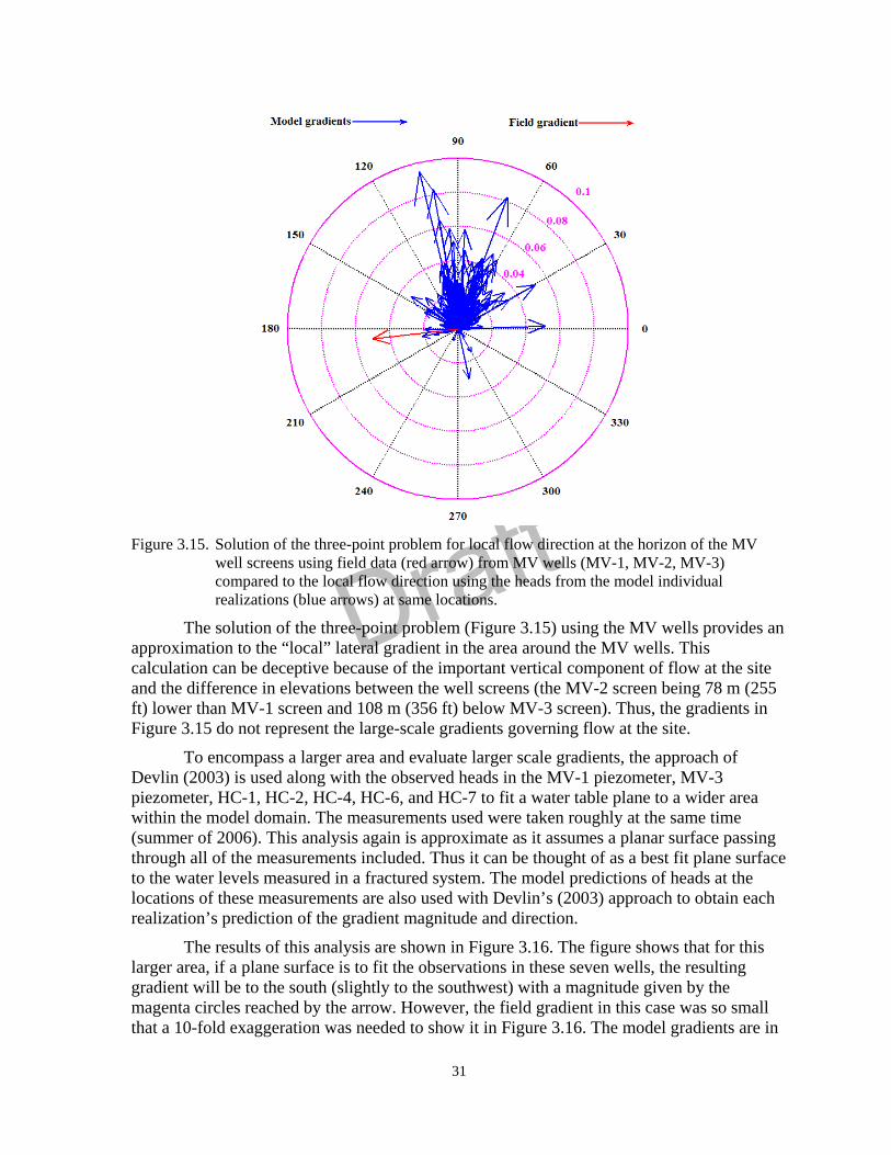
Draft

31

Figure 3.15. Solution of the three-point problem for local flow direction at the horizon of the MV

well screens using field data (red arrow) from MV wells (MV-1, MV-2, MV-3) compared to the local flow direction using the heads from the model individual realizations (blue arrows) at same locations.

The solution of the three-point problem (Figure 3.15) using the MV wells provides an approximation to the “local” lateral gradient in the area around the MV wells. This calculation can be deceptive because of the important vertical component of flow at the site and the difference in elevations between the well screens (the MV-2 screen being 78 m (255 ft) lower than MV-1 screen and 108 m (356 ft) below MV-3 screen). Thus, the gradients in Figure 3.15 do not represent the large-scale gradients governing flow at the site.

To encompass a larger area and evaluate larger scale gradients, the approach of Devlin (2003) is used along with the observed heads in the MV-1 piezometer, MV-3 piezometer, HC-1, HC-2, HC-4, HC-6, and HC-7 to fit a water table plane to a wider area within the model domain. The measurements used were taken roughly at the same time (summer of 2006). This analysis again is approximate as it assumes a planar surface passing through all of the measurements included. Thus it can be thought of as a best fit plane surface to the water levels measured in a fractured system. The model predictions of heads at the locations of these measurements are also used with Devlin’s (2003) approach to obtain each realization’s prediction of the gradient magnitude and direction.

The results of this analysis are shown in Figure 3.16. The figure shows that for this larger area, if a plane surface is to fit the observations in these seven wells, the resulting gradient will be to the south (slightly to the southwest) with a magnitude given by the magenta circles reached by the arrow. However, the field gradient in this case was so small that a 10-fold exaggeration was needed to show it in Figure 3.16. The model gradients are in

Draft

32

the same direction in some realizations and in the opposite direction (north-northeast) in other realizations. Some of the model realizations have larger magnitude and others have comparable magnitude to the field gradient. Therefore, on a larger scale, the model seems to be representing the measurement-inferred general slope of the water table in some realizations. However, the fractured nature of the site and the heterogeneity and connectivity of these fractures play a major role in determining where water is flowing.

0.2

0.4

0.6

30

210

60

240

90

270

120

300

150

330

180 0

Field GradientModel Gradients

Figure 3.16. Lateral gradient obtained by fitting a planar surface to the observed heads MV-1

piezometer, MV-3 piezometer, HC-1, HC-2, HC-4, HC-6, and HC-7 (red arrow) and corresponding gradients from the model individual realizations (blue arrows) at same locations. Field gradient (red arrow) is exaggerated with a factor of 10.

Combining all targets together, five out of 12 targets fall between the 2.5th and 97.5th percentiles of the model distributions for these targets. This gives a P2 value of 41.7 percent, which is between the 40 and 50 percent range shown in the decision tree (Figure 2.2). Given P1 = 13.2 percent and P2 = 41.7 percent, and based on the decision tree, the right-hand-side loop of the validation process (Figure 2.1) takes effect to see if the parameter distribution can

Draft

33

be adjusted by generating new realizations (see the discussion of Step 6a of the validation process in Section 2.1).

This could be achieved by using higher recharge values in the model (i.e., shifting the recharge distribution toward the high values) while keeping the same conductivity distribution. This would result in higher heads, thereby shifting the head distributions to the right-hand side (i.e., toward the high heads) in such a way that some or all of the head validation targets fall within the inner 95 percent of the model distribution of those targets. As a result, the P2 metric would have been increased to a value above 50 percent. The other metric, P1, would have also changed. The final outcome of such analysis is not known until the analysis is performed.

Before proceeding with the process, an important aspect influencing the above analysis and the values of P1 and P2 should be considered and evaluated. This aspect relates to the fact that the measured heads in the HC wells show temporal variations indicating that the Shoal system is transient, possibly as a result of the 1996 and 1999-2000 drilling and testing. Figure 3.16 shows the variation of the water levels measured in the HC wells over the years from 1999 to 2006. Water levels in many of the HC wells are still rising and the current values are different from what was used in the model calibration. Pohlmann et al.’s (2004) model was calibrated using the 1999 measurements in the HC wells. The MV data used for validation were collected in 2006. This time disconnect should be considered and can be handled in two ways, which are discussed in the following section.

3.3.3 Time Adjustment of Water Level Measurements

Hydrographs of water levels in the HC wells (Figure 3.17) indicate that water levels in some of these wells have not reached equilibrium. Wells HC-5 and HC-8 (not shown in Figure 3.17 because they are in a separate hydrologic block outside the model domain) appear to be at equilibrium, but these wells are completed much deeper in the system. The observations in the shallower HC wells, within the model domain, may record a site-specific trend reflecting a natural transient condition, or a drilling effect that has persisted for six to 10 years. Due to this rising trend, some of the current HC water level measurements are about 3 to 4 m higher than the values used in calibrating the Shoal model of Pohlmann et al. (2004). Compared to the model discretization scale (20 m) to which a single head value is assigned (or predicted), this difference is considered small. However, it may be impacting the model validation analysis. The time disconnect results from comparing a model that was calibrated based on 1999 measurements in the HC wells to measurements made in 2006 in the MV wells. With the transient conditions at the site, if one had drilled the MV wells and measured their water levels in 1999, those levels may have been lower than what was measured in 2006.

This time disconnect can be accounted for in two different ways. Either the model can be carried forward in time or the validation data can be projected backward in time. The first requires recalibrating the model to the 2006 HC measurements and rerunning the model based on the new calibration analysis. Subsequently, the 2006 MV data can be compared to the forward-projected model results. The second approach involves projecting the MV measurements backward in time using trend analysis of the transient hydrographs of the HC water level measurements. A trend analysis for the HC measurements can establish the slope of the rising water level hydrograph, which can then be used to project the MV

Draft

34

measurements back to 1999. This assumes the transient conditions and the rising water level trends are similar at the HC and the MV well locations, but is a simpler approach to implement than recalibrating the model.

Figure 3.17. Variation of water level measurements in the HC wells located within the Shoal model

domain (i.e., on the west side of the shear zone).

The hydrographs for wells HC-1, HC-2, and HC-4 indicate somewhat stable trends over the years (Figure 3.18). That is, the increasing trend has a monotonic pattern with no abrupt changes. The hydrographs of the water levels in HC-6 and HC-7 are dramatically impacted by the year-long tracer test and thus are not used in this trend analysis. Note that the other HC wells, HC-3, HC-5 and HC-8, are completed in a different hydrologic block, on the other side of a hydraulic barrier created by a shear zone. For HC-1 and HC-2, data on water levels are available from 1997 to present, whereas for HC-4, data are available only from late 1999. Measurements at HC-4 can only be made using a pressure gage and air pump in a bubbler line, and thus are more difficult to make and subject to higher uncertainty. Trend analysis using all available data (Figure 3.18a) yields slopes of 1.6700E-03, 1.1683E-03, and 1.3112E-03 m/day for HC-1, HC-2, and HC-4, respectively, with an average slope of 1.3832E-03 m/day. This average slope translates into an average rise in water level of about 0.51 m per year.

Draft

35

Figure 3.18. Trend analysis using the varying HC water level measurements: a) all data are used, and

b) only data from late 1999 to present are used.

Because the backward projection of the MV wells is intended to be from the present to the time of model calibration in1999, the trend analysis is repeated using only data from

a)

b)

Draft

36

late 1999 to the present (Figure 3.18b). The resulting slopes in this case are 9.5998E-04, 1.4821E-03, and 1.3112E-03 m/day for HC-1, HC-2, and HC-4, respectively, with an average slope of 1.2511E-03 m/day. This value is equivalent to about 0.46 m/year and is the value used to adjust the MV measurements to 1999 conditions. This slope yields a reduction of the measured head values of about 3.06 m for MV-1 and MV-3 and 3.00 m for MV-2 measurements (Table 3.4). The last column of Table 3.4 displays the backward-projected heads at the MV wells.

The R2 value of the linear regression conducted for HC-1 changed from 0.97 when all the record is used (Figure 3.18a) to 0.95 when the record from 1999-2006 is used (Figure 3.18b). Similarly, these values for HC-2 are 0.98 and 0.996, respectively. For HC-4, the record starts from 1999 and thus the value of R2 for HC-4 linear regression analysis is 0.84. This value is smaller than HC-1 and HC-2 values because of the large fluctuations at the early part of the water level record which are associated with the drilling effects.

It is important to note that the MV heads measured since the wells were drilled to the time this analysis was conducted (i.e., Spring 2007) showed a very strong positive correlation with the HC measurements during the same period. Table 3.5 shows the correlation matrix of wells MV-1, MV-3, HC-1, and HC-2. These are the wells for which simultaneous records exist during the specified period. As can be seen from the table, the MV measurements are highly correlated with the HC measurements, with correlation coefficients between 0.948 and 0.995.

Table 3.4. Predicted heads at MV wells using mean slope from reduced data set.

Mean slope (reduced data): 1.2511E-03 Mean date of HC-1 and HC-2 December 1999 measurements: 12/30/1999 11:53 PM

Date

Time

Julian Day

Measured Water Level

(m)

Days from 12/30/1999 11:53 PM

Backward- projected

Levels (m) MV-1 Main 09/12/2006 11:07 38,972.46 1,297.42 2,447.47 1,294.36 MV-1 Piezometer 09/12/2006 10:47 38,972.45 1,298.76 2,447.45 1,295.70 MV-2 Main 07/25/2006 15:51 38,923.66 1,296.08 2,398.67 1,293.07 MV-2 Piezometer 07/25/2006 16:11 38,923.67 1,257.88 2,398.68 1,254.88 MV-3 Main 09/12/2006 16:23 38,972.68 1,303.08 2,447.69 1,300.01 MV-3 Piezometer 09/12/2006 16:44 38,972.70 1,303.11 2,447.70 1,300.05

The values of seven validation targets are potentially affected by projecting the MV head values backward in time. These are the five head targets in the MV wells (three in the main wells and two in the piezometers of MV-1 and MV-3) and the lateral gradient magnitude and direction. However, the change in the latter two targets resulting from the projection is very minor and thus only the five head targets encounter significant change. The vertical gradients in MV-1 and MV-3 have not been affected, as the measurements in these two wells were reduced by the same amount.

Draft

37

Table 3.5. Correlation matrix showing the measurement correlation between MV and HC wells.

MV-1 MV-3 HC-1 HC-2MV-1 1MV-3 0.98885 1HC-1 0.99478 0.96851 1HC-2 0.98484 0.94803 0.9974 1

Using the 1999-projected MV measurements, the goodness-of-fit measures (using head data) discussed in Section 3.3.1 change. The comparison between the measures R2, d, and d1 obtained using the original measurements (refer to Figures 3.7 through 3.9) and their values using the projected heads is shown in Figure 3.19. As indicated earlier, the coefficient of determination, R2, is insensitive to additional differences. Thus when reducing all head targets by almost the same amount, the correlation-based measure, R2, does not change (compare Figures 3.19a and b). For the measures d and d1, the projected targets lead to higher values (Figure 3.19c through f), indicating better correspondence between the model and the targets. This will impact the composite scores of individual realizations, as discussed later in Section 3.4.

The P1 metric obtained using the projected heads is similar to the one obtained with the measured heads. The P1 values for the individual targets using the backward-projected heads are the same as shown previously in Table 3.3 except that target 3 (head measurement at MV-2 main well) changed from zero percent to 8 percent after the projection. For P2, a small change results from the projected heads. Figure 3.20 shows the values of the original heads and the backward-projected heads relative to the model-produced distributions of these targets. The original heads (red circles) were all outside the middle 95 percent of the model distribution. However, using the projected heads, the target head at MV-2 is within the middle 95 percent of the model distribution, and the one at MV-1 is very close, though still outside the middle 95 percent zone. This yields a value of 50 percent for P2 (6 targets out of 12 are within the middle 95 percent of the model distributions) as opposed to 41.7 percent using the original measurements.

The decision tree indicates that if P1 is less than 30 percent and P2 is 50 percent or more, one can tentatively deem the number of realizations with satisfactory scores sufficient (Figure 2.2). These are the realizations attaining composite scores that exceed a minimum threshold value. Determining if there are a sufficient number of satisfactory realizations can be finalized after evaluating the remaining performance measures (P3, P4, and P5) and developing the realizations’ composite scores and threshold value.

T he analysis presented in the following sections, which is related to the measures P3, P4, and P5, is based on the projected heads. Similar analysis is conducted using the measured heads in the MV wells with the results given in Appendix C. When integrating all the analysis and developing composite scores for model realizations, both sets of analyses (those using the projected heads and those using the measured heads) are used and the composite scores are compared.

Draft

R2 for each Realization Maximum R2 Using Measured Water Levels in MV Wells Using Backward-projected Water Levels in MV Wells

a)

b)

c) d)

e) f)

Figure 3.19. Comparison between goodness-of-fit measures, R2, d, and d1, obtained using head data from original MV measurements (a, c, and e) and corresponding backward-projected measurements (b, d, and f).

38

Draft

39

Figure 3.20. The MV head observations (red circles) and the backward-projected values (black

circles) relative to the distributions produced by the model at each of their respective locations. The suffix “W” indicates the main well casing and the suffix “U” indicates the piezometer installed in the annular space.

It should be remembered that the steady state assumption of the original Pohlmann et al.’s (2004) model is invalidated per the continuing change of the water levels in the HC wells. The backward projection of the MV water level measurements and the subsequent analysis discussed above are aimed at evaluating the model performance in the absence of the transient conditions or if the steady state assumption was correct. Put differently, had the MV wells been drilled and data collected in 1999, the validation analysis could possibly have resulted in declaring the number of realizations with satisfactory scores sufficient. This isolates the steady-state assumption from other model components such that the overall model performance in the absence of the invalidated steady-state assumption can be evaluated. If the overall performance is acceptable, then the central issue becomes the steady-state assumption and the implications of it being not true.

3.3.4 Applying the Stochastic Validation Approach of Luis and McLaughlin (1992), P3

This approach is applied here using the head data only. Details of the approach can be found in Luis and McLaughlin (1992) and also in Hassan (2003, 2004a, c). A brief description of the aspects related to the application to the Shoal model is presented here for completeness. The approach is based on the assumption that the flow model is used for predicting the distribution of hydraulic head in space, which describes the large-scale flow behavior of the system. Another assumption is that the observations made for the purpose of model validation are small-scale observations collected at sparse points in space and are assumed to be consistent with the steady-state assumption of the model. Only the first of these assumptions is met in the Shoal model. The steady state assumption is not validated as shown from the continuing rise of the water levels in the HC wells. The analysis here proceeds under the assumption that the transient state at the site was not an issue as stated

Draft

40

earlier. This is done by the backward projection of the MV data. Thus the stochastic validation analysis of Luis and McLaughlin (1992) is applied to the model.

Under these assumptions, the differences between predicted and measured head values can be attributed to three error sources: (1) measurement errors, which represent the difference between the true values and measured values of hydraulic head; (2) spatial heterogeneity, which represents the difference between the large-scale trend (or smoothed head) that the model is intended to predict and the true small-scale, actual values of head; and (3) model error, which represents the difference between the model prediction and the actual smoothed trend. Figure 3.21 shows a schematic representation of these error sources, where an actual, fluctuating (due to heterogeneity) head distribution, hj, with a large-scale trend, jh , is shown in conjunction with a hypothesized stepwise distribution representing model prediction, jh .

The jth measurement residual, εj, observed at location xj (for j = 1, ..., N), where N is the total number of head measurements used for validation, can be written in terms of three components of the error or the mismatch. This leads to the equation

)]ˆ(ˆ[][][ * ηε jjjjjjj hhhhhh −+−+−= (3.14)

where the first term between the square brackets represents measurement error, the second bracketed term represents the effect of geologic heterogeneity, and the last term represents the model error.

If the model is valid, the hypothesis that the model prediction is equal to the smoothed, large-scale values should be accepted. This is equivalent to accepting that the model error term in Equation (3.14) is zero. In statistical terms, the following null hypothesis is considered:

jj

jj

hh

hh

≠

=

)ˆ(ˆ,tsignificaniserrorModel:H

)ˆ(ˆ,negligibleiserrorModel:H

1

0

η

η (3.15)

Draft

41

Figure 3.21. Schematic representations of the actual head distribution, large-scale trend, and stepwise

model prediction (A), and the decomposition of the measurement residual into three error sources or components (B). Subplot (B) is an enlargement of the circled section in subplot (A).

Luis and McLaughlin (1992) proposed several tests that can capture the different aspects of model evaluation. They proposed a quantitative approach to determine whether statistics such as the sample mean and covariance of the residuals are consistent with hypothesis H0 in (3.13). When the hypothesis is true, it can be shown that the desired measurement residual variance can be written as

222*

jj hh σσσ ε += (3.16)

Draft

42

where 2jεσ is the measurement residual variance, 2

*hσ is the measurement error variance

(human error, device error, etc.), and 2jhσ is the head variance stemming from geologic

heterogeneity. The head variance, 2jhσ , in (3.14) plays a key role in this approach since it

defines how much variability one should expect around the model’s predictions when the model structure and measurements are both perfect. In other words, this variance establishes a type of lower bound on the model’s ability to predict point values of head (Luis and McLaughlin, 1992). The head variance can be derived from the results of the flow model and evaluated at each node of the discretized domain. Equation (3.16) can then be used to evaluate the measurement residual variance under the assumption that H0 is correct. One can thus test the assumption that the mean residual is zero and use the mean squared residual (Equation [3.16]) to test the null hypothesis H0 in Equation (3.15).

3.3.4.1 Mean Residual Test

If the null hypothesis is true (i.e., the model is predicting correctly the desired large-scale trend), a sample mean computed from many measurement residuals should be close to zero. This implies a test of the following form:

.1

:statisticTest

0≠,tsignificanisresidualMean:H

0,negligibleis residualMean :H

1

1

0

j

jN

j

j

j

Nm

εε σ

ε

ε

ε

Σ=

=

= (3.17)

The null hypothesis, H0, is true if vm <ε , where v is a test threshold selected to give the desired two-sided type I error probability (or significance level, α). The null hypothesis, H0, in Equation (3.17) is equivalent to H0 in Equation (3.15). If it is assumed that εm is normally distributed (based on the central limit theorem), the threshold value may be obtained from a standard normal probability table (Luis and McLaughlin, 1992).

Using the backward-projected five head measurements from MV-1, MV-2, and MV-3, this hypothesis test is conducted for each individual realization of the Shoal model. First, the 1,000 realizations are used to compute the head variance at the locations of the five head measurements. These variances are denoted as 2

jhσ in Equation (3.16), where

j = 1, 2, …, 5. The measurement error variance term, 2*hσ , needed in Equation (3.16)

represents the errors associated with the field observations. To find this value, assume that there is a 95-percent confidence that the true head at any of the measured head locations in the three wells is within ± 0.3 m (i.e., ± 1.0 ft) of the observed head. If it is further assumed that a normal distribution applies, then the 95-percent confidence interval means that the interval from [the measured head value - 1.96 *h

σ ] to [the measured head value + 1.96 *hσ ]

is equivalent to 0.3 × 2 = 0.6 m. This implies that 1.96 *hσ = 0.3, thereby giving a value of

0.02343 for the measurement error variance, 2*hσ . Equation (3.15) is then used to obtain

2jεσ at each of the nine locations where head is measured.

Draft

43

To conduct the hypothesis test according to Equation (3.17), the test statistic, mε, is computed for each realization, where εj is obtained as the difference between the head prediction of the current realization and the measured head for each measurement location j = 1, 2, …, 5. This test statistic is compared to the critical value of the standard normal variate, Z, at an exceedence probability of 0.975. This is based on a two-tail test at a 95-percent confidence level or a 5 percent significance level. The results of this hypothesis testing are shown in Figure 3.22a. Among the 1,000 model realizations, the test statistic, mε, is smaller than the critical Z value in 577 realizations, and thus the null hypothesis (Equation [3.15] or [3.17]) is accepted (or more accurately cannot be rejected) in the 577 realizations. This indicates that the model prediction of the heads in these realizations do represent the large-scale trend inferred from the field measurements.

Figure 3.22. Results of the hypothesis testing formulated according to the stochastic validation

approach of Luis and McLaughlin (1992) using backward-projected heads: a) values of the test statistic (mε) that are smaller than the critical Z value indicate accepting the null hypothesis that model residual is negligible, and b) values of the test statistic (χ2) that are smaller than the critical χ2 value indicate accepting the null hypothesis.

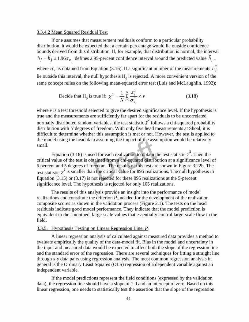
Draft

44

3.3.4.2 Mean Squared Residual Test

If one assumes that measurement residuals conform to a particular probability distribution, it would be expected that a certain percentage would lie outside confidence bounds derived from this distribution. If, for example, that distribution is normal, the interval

jjj hh εσ96.1ˆ ±= defines a 95-percent confidence interval around the predicted value jh ,

where jεσ is obtained from Equation (3.16). If a significant number of the measurements *

jh lie outside this interval, the null hypothesis H0 is rejected. A more convenient version of the same concept relies on the following mean-squared error test (Luis and McLaughlin, 1992):

Decide that H0 is true if: vN

j

jN

j<Σ=

= 2

2

1

2 1

εσε

χ (3.18)

where v is a test threshold selected to give the desired significance level. If the hypothesis is true and the measurements are sufficiently far apart for the residuals to be uncorrelated, normally distributed random variables, the test statistic χ

2 follows a chi-squared probability distribution with N degrees of freedom. With only five head measurements at Shoal, it is difficult to determine whether this assumption is met or not. However, the test is applied to the model using the head data assuming the impact of the assumption would be relatively small.

Equation (3.18) is used for each realization to obtain the test statistic χ2. Then the

critical value of the test is obtained from a chi-squared distribution at a significance level of 5 percent and 5 degrees of freedom. The results of this test are shown in Figure 3.22b. The test statistic χ

2 is smaller than the critical value for 895 realizations. The null hypothesis in Equation (3.15) or (3.17) is not rejected for these 895 realizations at the 5-percent significance level. The hypothesis is rejected for only 105 realizations.

The results of this analysis provide an insight into the performance of model realizations and constitute the criterion P3 needed for the development of the realization composite scores as shown in the validation process (Figure 2.1). The tests on the head residuals indicate good model performance. They indicate that the model prediction is equivalent to the smoothed, large-scale values that essentially control large-scale flow in the field.

3.3.5. Hypothesis Testing on Linear Regression Line, P4

A linear regression analysis of calculated against measured data provides a method to evaluate empirically the quality of the data-model fit. Bias in the model and uncertainty in the input and measured data would be expected to affect both the slope of the regression line and the standard error of the regression. There are several techniques for fitting a straight line through x-y data pairs using regression analysis. The most common regression analysis in general is the Ordinary Least Squares (OLS) regression of a dependent variable against an independent variable.

If the model predictions represent the field conditions (expressed by the validation data), the regression line should have a slope of 1.0 and an intercept of zero. Based on this linear regression, one needs to statistically test the assertion that the slope of the regression

Draft

45

line is unity and that the intercept of the line is zero. Hypothesis testing can be used for this purpose with the null and alternative hypotheses expressed as

1Slope:H

1Slope:H

1

0

≠

= (3.19)

The test statistic is ((Slope-1) ÷ standard deviation of the slope). This statistic is to be compared to the critical value of the t-distribution at (N - 2) degrees of freedom (N is the number of data pairs) and at the α level of significance, )501,2( α⋅−−Nt . If the absolute value of the test statistic exceeds the critical value, the null hypothesis is rejected.

In a similar manner, the null hypothesis of a zero intercept can be examined. Assuming b is the intercept of the linear regression line, the intercept hypothesis test is formulated as

0:H

0:H

1

0

≠

=

b

b (3.20)

The test statistic is ((b-0) ÷ standard deviation of the intercept). This statistic is to be compared to the critical value of the t-distribution at (N - 2) degrees of freedom and at the α level of significance, )501,2( α⋅−−Nt . If the absolute value of the test statistic exceeds the critical value, the null hypothesis is rejected. Failing to reject both null hypotheses does not necessarily mean the model is free of biases, it only means that this analysis fails to identify any bias (Flavelle, 1992).

Figures 3.23 and 3.24 exhibit the testing results for the slope and the intercept, respectively. For the slope results, the unit-slope hypothesis is accepted for 90 realizations using the head data, 895 realizations using the conductivity data, and 486 realizations using gradient data. In other words, for the head regression analysis, 90 realizations had a regression line that is statistically not significantly different from 1.0. Similarly, for conductivity regression analysis and the gradient analysis, 895 and 482 realizations, respectively, had a regression line slope that is statistically not significantly different from 1.0. For the zero intercept tests, the null hypothesis is accepted for 91 realizations when using head data. For the hydraulic conductivity data, 872 of the 1,000 zero-intercept tests were accepted, and 947 of the 1,000 head gradient zero-intercept tests were also accepted.

It is important to look at multiple tests and evaluate the different aspects of each model realization in different ways. Some of the tests may give a false indication about performance, but the collective results of multiple tests will increase the odds that the correct decision about model performance is reached. The results of the hypothesis testing on the regression line lead to the fifth measure, P5, needed in the validation process (Figure 2.1) to develop the realization composite scores.

Draft

46

Figure 3.23. Results of hypothesis testing on the slope of the linear regression line using head data (a), hydraulic conductivity data (b), and gradient data (c).

Draft

47

Figure 3.24. Results of hypothesis testing on the intercept of the linear regression line using head data (a), hydraulic conductivity data (b), and gradient data (c).

3.3.6 Testing Model Structure and Failure Possibility, P5

Three tests are performed for the model as a whole. First, the fracture data obtained from the MV wells are compared to the original data used in the Shoal model. Second, the relation between the conductivity variance and the head variance for each realization is compared to the field value to see whether the field condition was encompassed by the range of stochastic model realizations. The field value refers to the head variance and the conductivity variance computed from the MV measurements. This field value is compared to the similarly computed values for the 1,000 model realizations. Third, the presence of Shoal test-related radionuclides farther away from the cavity than predicted is considered a failure scenario and is therefore checked through this validation process.

Fractures and faults were originally characterized using video logs, ATV logs, and radar logs of the HC boreholes, as well as data from surface mapping of visually observable features (Pohlmann et al., 2004). The location, orientation and the dip of fractures were

Draft

48

estimated using these observations. The orientation data provided a multi-modal distribution (Pohlmann et al., 2004; Figure 3.7) that would have been overly smoothed if fitted to a simple distribution. Given this fact and the strong impact on flow and transport believed to result from the actual heterogeneous, discrete, but uncertain, fracture network, an empirical distribution was used to describe the detailed orientation and dip distributions. Thus, data on about 722 fractures (orientation and dip) were randomly sampled in Pohlmann et al.’s (2004) model and used in generating the stochastic fracture maps. These maps formed the basis for the Shoal flow model. The data on these 722 fractures can be compared to the data obtained from the MV wells.

As stated earlier, fracture orientation and dip data were obtained through ATV logs in the MV wells. The televiewer logging and the data interpretation were conducted by Colog, Borehole Geophysics and Hydraulics, Inc. as a subcontractor to SNJV. About 862 fractures were identified in the three MV boreholes and data on their dip and orientation are provided by Colog. This allows the comparison to the fracture data set available for the 722 fractures identified from the logging of the HC boreholes.

Figure 3.25 shows contour plots of all fracture orientations obtained from the HC wells as well as from the three MV wells. Equal area projection on the lower hemisphere is used for creating these contours. It is clear that data from MV-2 closely resemble the data obtained from the HC wells and used in the model. Wells MV-1 and MV-3 fracture data do not as closely resemble the HC data. It should be noted that the MV-2 well is deeper than the other two wells and as such it samples more fractures at its location. This set of fractures resembles well the set of fractures used in the original Shoal model.

Figure 3.26 compares the histograms of fracture dip direction and fracture dip angle from all MV wells (separately and combined) to what was used in the Shoal model. The dip direction distribution used in the model was bimodal with two modes: one at about 100 degrees and the other at about 300 degrees from magnetic north. All three wells indicate the existence of the mode at around 300 degrees, but only MV-2 indicates a mode (or a clustering) close to 100 degrees. MV-1 and MV-3 data show the existence of a mode near 200 degrees for the dip direction. Thus, overall, a reasonable correspondence exists between the fracture dip direction data from MV-2 and what was used in the Shoal model.

Draft

49

Figure 3.25. Fracture orientation comparison between data from HC wells (top left plot) and MV-1 data (top right), MV-2 (lower left), and MV-3 (lower right) through equal area projection, lower hemisphere.

Draft

50

0 100 200 300 4000

50

100

Azimuth (degrees from magnetic North)

Freq

uenc

y Data Used in Model

Dip Direction Distribution

0 20 40 60 800

50

100

Dip (degrees))

Freq

uenc

y Data Used in ModelFracture Dip Distribution

0 100 200 300 4000

50


Freq

uenc

y MV-1 Data

0 20 40 60 800

50

Dip Angle (degrees from horiz.)

Freq

uenc

y MV-1 Data

0 100 200 300 4000

20

40


Freq

uenc

y MV-2 Data

0 20 40 60 800

20

40

Dip Angle (degrees from horiz.)Fr

eque

ncy MV-2 Data

0 100 200 300 4000

20

40


Freq

uenc

y MV-3 Data

0 20 40 60 800

20

40


Freq

uenc

y MV-3 Data

0 100 200 300 4000

50

100


Freq

uenc

y Data from all MV Wells

0 20 40 60 800

50

100


Freq

uenc

y Data from all MV Wells

Figure 3.26. Empirical distributions of fracture dip direction and fracture dip angle for the original Shoal model (cyan histograms) and as obtained from the MV wells (yellow histograms).

The distributions of the dip angle show even better correspondence than the dip direction distributions. The data used in the model and data from MV-1 and MV-3 indicate the same distribution; a left skewed distribution with a modal value around 60 to 70 degrees. Well MV-2 data indicate more of a uniform dip distribution in the range of 5 to 80 degrees. When adding data from all three MV wells, the resulting distribution looks similar to the original data used in the model, which provides an important validation aspect for the model.

To quantitatively compare the dip direction and dip angle data used in the model to those collected from the MV wells, the mean and standard deviation of these different data sets are obtained and compared (Table 3.6). Both individual MV data sets and the collective

Draft

51

set of all MV wells give mean and standard deviation values close to the value obtained from the original model data for the dip angle. However, for the dip direction, the MV data show a distribution with a higher mean but same standard deviation as used in the Shoal model.

Table 3.6. Mean and standard deviation of fracture strike and fracture dip for the data used in the original model and for the data obtained from the MV wells.

Mean Std. Dev. Mean Std. Dev.

Model 144.70 93.58 61.10 13.43MV-1 198.62 86.93 57.31 20.67MV-2 172.41 90.29 60.14 17.24MV-3 196.16 93.72 40.56 20.95All MV Wells 189.80 91.04 52.18 21.62

Fracture StatisticsDip direction Dip angle

The second step in testing model structure is the comparison of the measured head and hydraulic conductivity variances with the model-predicted variances. This gives an overall idea of how the model structure compares to what is found from the validation data. The model predictions for the five head validation targets and the three hydraulic conductivity targets are analyzed for each realization. The variance of the five head values,

2hσ , is obtained for the measured heads and for the modeled heads of each realization.

Similarly, the three hydraulic conductivity values measured in the validation wells are used to compute 2

log Kσ , and a similar value is computed for each realization. The results are plotted in Figure 3.27. Ideally, the field point would plot within the cloud produced by the model realizations. This occurs for the Shoal model where the validation result (red circle) is located within the results of the model realizations. This is another positive result regarding the performance of the model in relation to the validation data.

Figure 3.27. Relation between head and hydraulic conductivity variances as obtained from the model

and the validation data.

Draft

52

The third and final check of model structure and failure possibilities is for the presence of radionuclides (e.g., tritium) above background levels in the wells. Based on the analysis of tritium in samples collected from the three wells, no evidence is found of test-related radionuclides above natural background. Tritium was detected in MV-3, but the concentration was near atmospheric background levels (13 ± 9 pCi/L; Lyles et al., 2006). This validates the predictions of the Shoal transport model regarding the absence of transport to the locations of the MV wells at the present time.

3.4 Developing Composite Scores for Model Realizations (Step 5)

The calibration and validation analyses performed in the previous sections can be categorized into two types. One type is applicable to individual realizations (e.g., goodness-of-fit measures, realizations scores (Sj), stochastic validation approach, hypothesis testing on linear regression results) and the other is applicable to the model as a whole (e.g., P1 and P2 measures, model structure test through variance relations, fracture data comparisons). The first type of analysis pertaining to the individual realizations is used to develop a composite score for each realization and determine the number of acceptable realizations. To determine this number, a threshold needs to be determined (see Appendix A) above which a realization composite score can be considered satisfactory. This number of realizations along with P1, P2, and the failure analysis results (i.e., variance results, fracture distribution (Figure 3.28), and radionuclide sampling results in the MV wells) will guide the final decision regarding the model assessment. It should be remembered that Figure (2.2) indicated tentatively that there are a sufficient number of realizations based on a P1 value of 13.2 percent and a P2 value of 50 percent for the backward-trended head values.

A realization in a perfect world would have a high calibration weight (the GLUE weights shown in Figure 3.5), values for the goodness-of-fit measures R2, d, and d1 as close to 1.0 as possible, accepted hypothesis testing on the aspects related to the residuals and the linear regression line, and scores Sj as close to 1.0 as possible. To quantify these aspects, the following scoring system is used:

1. The calibration weight is divided by the maximum GLUE weight attained. This gives the single realization with the maximum GLUE weight a score of 1.0 and all other realizations get scores less than 1.0 on the calibration result.

2. The goodness-of-fit results for different data sets are used as obtained, because R2, d, and d1 have values between zero (worst performance) and 1.0 (best performance).

3. The results of hypothesis testing are binary-type results (i.e., the null hypothesis is either accepted or rejected). These are converted to a binary [0, 1] system. A score of zero is given if the hypothesis is rejected and a score of 1.0 is given if the hypothesis is accepted.

4. The realization scores on the different validation targets, Sj, are used as obtained because these values range from zero to 1.0.

Because the head values have been used the most in the above tests, their results may outweigh the other data (conductivity and gradient data) in this scoring system. Thus, to avoid this overweighing, three average scores are developed from which the final composite score is obtained. These three averages are: 1) the average score of all tests relying on head data from the MV wells, 2) the average score of all tests relying on the conductivity data, and

Draft

53

3) the average score of all tests relying on the gradient data. These averages are added to the calibration score (see item number 1 in the previous list) to develop the final composite score for each realization. Based on this scheme, the maximum possible score (i.e., the perfect score) for any realization is 4.0. However, this is practically unachievable because it implies perfect results on all model tests including perfect calibration results. Thus, although the maximum value is theoretically 4.0, the minimum acceptable value is arbitrary and it needs to be determined in a justifiable manner. This is discussed in Appendix A.

Table 3.7a displays the different tests and the scoring system for the first 15 realizations of the Shoal model, and Table 3.7b shows the realization scores, Sj, as computed using Equation (3.9) for each of the 12 validation targets. To develop the composite scores, all tests that rely on the head measurements are averaged to provide a single score for each realization ranging from 0.0 to 1.0. Similarly, all tests using the hydraulic conductivity data are averaged to a single score and the same is done for the model tests based on the head gradient data. Table 3.8 shows these three averaged scores, the calibration scores, and the final composite scores for the first 15 realizations of the Shoal model. These realizations attained scores ranging from 1.31 to about 2.1. The scores for all model realizations are shown in Figure 3.28.

The composite scores are obtained based on the backward-projected MV water levels (Figure 3.28a) and the actual, 2006-measured water levels (Figure 3.28b). First, it is observed that minor differences exist between the two sets of scores. The low scores (close to 1.0) are impacted the most by the backward projection. Second, none of the realizations attained a score below 1.0 while many realizations attained scores above 2.0.

The determination of the acceptable or satisfactory score for any realization of the Shoal model is made using a jackknife approach (Appendix A). This approach gives an average score of about 2.041, assuming one of the model realizations exactly matches reality (i.e., represents the field data). Given that the field data collected for the validation analysis at any site are very unlikely to exactly match any of a model’s realizations, a value of 75 to 90 percent of the mean value of 2.041 can be considered as the threshold for satisfactory realization scores. If one, on average, obtains 2.041 for the composite realization score when one of the model realizations is assumed to match real field conditions, one can safely assume the model realization is generally acceptable if its composite score obtained using the actual validation data is above 75 percent of this value.

Draft

54

Figure 3.28. Composite score for all model realizations, including those presented in Table 3.8, using

backward-projected heads (a) and original head measurements (b). The line of the ideal score is shown for comparison.

a)

b)

Draft

Table 3.7a. Example of the scoring system used to develop a composite score, showing results from 15 of the 1,000 realizations.

head data

conductivity data

gradient data

head data

conductivity data

gradient data

head data

conductivity data

gradient data

m ε χ 2 head data

conductivity data

gradient data

head data

conductivity data

gradient data

1 0.0051767 0.3057 0.9186 0.9014 0.4932 0.0300 0.5101 0.4156 0.0336 0.4660 1 1 0 1 0 0 1 12 0.0039242 0.2250 0.4819 0.6014 0.3252 0.6910 0.5265 0.2091 0.3778 0.4449 0 1 0 1 1 0 1 13 0.0073342 0.4792 0.5392 0.9954 0.7412 0.3156 0.0000 0.5963 0.1767 0.0000 1 1 1 1 0 1 1 04 0.0015334 0.3755 0.2661 0.9659 0.2608 0.4452 0.4514 0.1532 0.2232 0.4291 0 0 0 1 0 0 1 05 0.0050185 0.4685 0.6884 0.3092 0.4907 0.0249 0.4367 0.3909 0.0132 0.3993 1 1 0 1 0 0 1 16 0.0029326 0.2796 0.0038 0.4600 0.3934 0.0632 0.4318 0.2618 0.0388 0.4306 1 1 0 1 1 0 1 17 0.0027761 0.4251 0.3946 0.8285 0.3765 0.3540 0.5192 0.2631 0.2661 0.4612 1 1 0 1 0 0 1 18 0.0015536 0.0029 0.0317 0.0135 0.2675 0.3838 0.4708 0.1596 0.2480 0.4490 0 0 0 1 0 0 1 19 0.0028815 0.3524 0.1681 0.5973 0.4603 0.2927 0.6282 0.3017 0.3518 0.4298 1 1 0 1 1 0 1 1

10 0.0039136 0.2709 0.8645 0.8636 0.4049 0.0260 0.7926 0.3257 0.0175 0.6202 1 1 0 1 1 0 1 111 0.0066609 0.5738 0.9810 0.9979 0.5147 0.4169 0.5059 0.4653 0.2050 0.4733 1 1 0 1 0 0 1 112 0.0017941 0.3209 0.8761 0.6927 0.2914 0.1749 0.5646 0.1804 0.1801 0.4826 0 1 0 1 1 0 1 113 0.0039303 0.0433 0.0030 0.7105 0.4539 0.3764 0.5230 0.3420 0.2499 0.4853 1 1 0 1 0 0 1 114 0.0018372 0.5151 0.2104 0.2299 0.3183 0.0363 0.4837 0.1892 0.0149 0.3947 0 1 0 1 1 0 1 115 0.0022775 0.0970 0.1374 0.5184 0.4353 0.4869 0.4227 0.3017 0.2898 0.3779 1 1 0 1 0 0 1 0

d 1

Realization #

R 2 dHypothesis testing on

regression line [Slope = 1.0 test]

Hypothesis testing on regression line

[Intercept = 0.0 test]

Residual tests (Luis and

McLaughlin, 1992)

)|( ΘYrr

mL

Table 3.7b. The rest of the scoring system used to develop a composite score. Sji values for the 12 validation targets (i = 1, 2, …, 12) for 15 (j = 1, 2, …, 15) of the 1,000 realizations are shown.

MV-1 Well

MV-1 Piez

MV-2 Well

MV-3 Well

MV-3 Piez

MV-1 Well

MV-2 Well

MV-3 Well

Lateral Gradient

Gradient Direction

1 0.9874 0.9591 0.9972 0.7329 0.8374 0.9796 0.9201 0.9931 0.7292 0.9995 0.1722 0.61992 0.7074 0.6299 0.7472 0.2996 0.5129 0.9426 0.9840 0.9769 0.7144 0.9954 0.2387 0.37113 0.9614 0.9970 0.9497 0.7322 0.9995 0.8742 0.8550 0.6999 0.4730 0.4187 0.3869 0.84754 0.3829 0.3239 0.4299 0.1294 0.3097 0.7736 0.8265 0.9997 0.7490 0.9974 0.1206 0.65875 0.9752 0.9378 0.9939 0.6997 0.8383 0.9804 0.6249 0.7659 0.7121 0.9923 0.1312 0.67766 0.8297 0.7919 0.8841 0.4717 0.6688 0.9840 0.9767 0.7137 0.8985 0.9942 0.1208 0.96047 0.8592 0.7966 0.9025 0.4569 0.6419 0.9846 0.7972 0.9557 0.7423 0.9984 0.1993 0.33568 0.4315 0.3608 0.4860 0.1517 0.3282 0.9661 0.8055 0.9434 0.6967 0.9997 0.1206 0.36559 0.9202 0.8780 0.8765 0.5532 0.7796 0.9973 0.9920 0.6916 0.8163 0.9614 0.5576 0.597610 0.9708 0.9255 0.9575 0.5626 0.7122 0.9732 0.7380 0.9191 0.6538 0.9999 0.6466 0.438511 0.9969 0.9794 0.9999 0.7910 0.8714 0.8564 0.8588 0.8847 0.7446 0.9999 0.1566 0.753612 0.5852 0.4852 0.6084 0.2172 0.4007 0.9748 0.4831 0.8955 0.5706 1.0000 0.2543 0.435713 0.9523 0.9229 0.9707 0.6312 0.7708 0.9696 0.7998 0.9461 0.8606 0.9990 0.1942 0.564514 0.5965 0.5271 0.5984 0.2549 0.4946 0.9800 0.8127 0.7147 0.7597 0.9817 0.2501 0.650115 0.9062 0.8889 0.9217 0.5258 0.7580 0.9336 0.8433 0.9977 0.9643 0.9632 0.2638 0.4905

Realization # j

Head Targets Conductivity Targets

S ji

Gradient Targets

1∂/∂ Sh 3∂/∂ Sh

55

Draft

56

Table 3.8. Composite scores based on the calibration scores and the three averaged scores.

Realization #

Calibration score

Average score based on head

data

Average score based on

conductivity data

Average score based on

gradient data Total score

1 0.005177 0.6440 0.7344 0.5998 1.9834 2 0.003924 0.3880 0.8068 0.6547 1.8534 3 0.007334 0.8714 0.6826 0.3468 1.9081 4 0.001533 0.1971 0.6918 0.4858 1.3762 5 0.005019 0.6496 0.6372 0.5176 1.8094 6 0.002933 0.5484 0.5975 0.6996 1.8484 7 0.002776 0.5601 0.7190 0.5649 1.8469 8 0.001554 0.1823 0.6723 0.4573 1.3135 9 0.002881 0.5935 0.6867 0.7320 2.0151

10 0.003914 0.5942 0.6923 0.7795 2.0699 11 0.006661 0.6827 0.7753 0.6258 2.0905 12 0.001794 0.3408 0.6981 0.6667 1.7074 13 0.003930 0.5906 0.6681 0.5930 1.8556 14 0.001837 0.3745 0.5961 0.6389 1.6113 15 0.002277 0.5695 0.7111 0.4445 1.7274

3.5 Final Assessment of Model Adequacy (Step 6) The decision of Step 6 of the validation process pertains to the number of realizations

with satisfactory scores. This decision is to determine whether the number of realizations with satisfactory scores is sufficient (thus building confidence in the original model – Step 6b) or insufficient, indicating that the original model needs adjustment (Step 6a) or revision (Step 6c). Based on the decision tree of Figure 2.2, the conclusion was tentatively made earlier that there are sufficient realizations with satisfactory scores. This was based on an average P1 value (over all targets) of about 13.2 percent and a P2 value of 50 percent (for the backward-trended data). Although the decision tree indicates that the decision regarding the model is that there are sufficient realizations with acceptable scores, the determination of the threshold of acceptable scores and the determination of the number of realizations exceeding this threshold relies on all validation tests and evaluations as detailed in Figure 2.1.

The jackknife approach discussed in Appendix A determined that one could take the threshold for acceptable scores as 75 percent of the mean of the 1,000 mean scores. If it is desired to have a more conservative threshold, then 90 percent of the mean of the 1,000 mean scores can be used instead. These yield the threshold values of 1.53 and 1.84, respectively. Therefore, if any realization attains a composite score higher than 1.53, it is considered acceptable or having a satisfactory score. In the conservative approach, the realization composite score has to exceed 1.84 for it to be satisfactory. Using these thresholds, it is found that 458 realizations attained scores higher than 1.84 and 818 realizations attained scores higher than 1.53 for the analysis using the backward trended heads.

Draft

57

As stated earlier, the validation analysis was conducted from start to end using both the original 2006 measurements in the MV wells as well as the backward-projected heads. Table 3.9 compares the number of realizations attaining scores higher than the threshold value in both cases and using the 75 percent and 90 percent thresholds. When using the original heads, the numbers of realizations above the threshold change from 818 and 458 to 709 and 284. The acceptable realizations can be used for further analysis and uncertainty reduction.

Table 3.9. Number of realizations attaining scores higher than the threshold when using original and backward-projected MV heads.

Score threshold 75% of 2.041 (1.53) 90% of 2.041 (1.84)

Using observed MV heads 709 284 Number of acceptable realizations

Using backward-projected MV heads 818 458

The number of acceptable realizations needed to consider the overall model validated is subjective, but the numbers attained for the 75% criterion are probably acceptable to most evaluators, whether using the observed or projected heads. As a consequence, the adequacy of the overall model structure and performance could be presumed, confirmed by the overall model tests including fracture data comparisons, and absence of test-related radionuclides in the MV wells. Whether or not there are a sufficient number of acceptable realizations using the 90% criterion would probably elicit greater debate, particularly for the observed heads.

A major caveat to any determination of acceptance is the invalidated steady-state assumption of the model. During the two modeling stages of the site (Pohll et al., 1998; Pohlmann et al., 2004, the model of which was completed a couple of years earlier than the report was published), the transient conditions observed in the HC wells were thought to be short term effects of the drilling activities. But these effects have persisted for years (note that wells HC-1 through HC-4 were drilled with a direct circulation technique that stressed the wells more than the reverse circulation method used in HC-5 through -8, but that HC-6 and HC-7 were used in a year-long pumping tracer test). The change in the water level between 1999 and 2006, found to be about 3 m in the trend analysis discussed in Section 3.3.2.1, is within the uncertainty range of the model output (Figure 3.29) at the locations of the HC wells used for calibration, except at HC-1 where the current water level is outside the inner 95 percent of the model distribution for the head. These uncertainty bounds may alleviate concern regarding the invalidated steady-state assumption. If the comparison between the contaminant boundary obtained from the reduced set of realizations (ignoring the steady-state assumption) and that obtained from the original model (see Section 4) is acceptable to NDEP (Steps 6b and 7a of the validation process), the concern regarding transient effects could be addressed by monitoring water levels. This is advisable as it would provide an early warning of major deviation from the model if the trend persists for many future years. In such a case, the model should be revisited and evaluated. If the rising water levels stabilize in the near future, then the violation of the steady-state assumption over the past years is already compensated by the model uncertainty range (Figure 3.29). In this case,

Draft

58

revising the model and correcting for this assumption will not yield dramatically different results compared to the 2004 model of Pohlmann et al.

Figure 3.29. The HC water level measurements of 2006 (red circles) and the 1999 calibration values

(black circles) relative to the distributions produced by the model at each of their respective locations. GLUE calibration weights developed in Pohlmann et al. (2004) are used to determine the model’s 2.5th, 50th, and 97.5th percentiles (green triangles).

One of the important aspects of the validation process is that it is considered a long-term and iterative confidence building process. It cannot ensure acceptable prediction or quality of the model. Rather, it provides an important safeguard against faulty models or inadequately developed and tested models. The validation process aims at providing confidence that the model is valid for it intended use and it is not required to prove that the model is an exact representation of reality.

The results of the validation analysis of the Shoal model indicate possibly acceptable performance but not necessarily exact representation of reality. None of the tests or validation data invalidated the conceptual or structural components of the Shoal model, except for the steady-state assumption. The discrepancies between some of the model realizations and the validation data are expected for any stochastic model. By its very definition, these stochastic models cover a wide range of site characteristics and flow and transport systems. It is thus unexpected, and also not required, that all the model realizations match the field data. If that happens, it just indicates that model realizations are all the same or very similar.

The general pattern of hydraulic head across the site remains similar between the data used for calibration and those observed in 2006 (Figure 3.30). Head values are within several meters of one another across the site, describing a water table with low relief beneath Gote Flat. Downward vertical gradients are also observed in the MV data. Thus, groundwater flow is downward and lateral gradients, while obscured by different screen elevations and the effects of fracture flow (Figure 3.31), are driven primarily by forces beyond the model boundaries.

Draft

59

Figure 3.30. A) Water levels in Shoal boreholes and characterization wells used for model

calibration, along with estimated water levels in the MV wells, trended to the 1999 calibration time period. B) Hydraulic head measurements from 2006.

A)

B)

Draft

60

Region outside flow domain

Figure 3.31. Head distribution for one realization of a Shoal flow model, showing discontinuous

pattern related to fracture flow and downward gradients. Heads are shown in meters relative to sea level.

An important test on the final assessment of the model is to compare the acceptable realizations (whether the 458 or the 818 realizations for the backward projected heads) to their performance on the calibration results (Figure 3.5) documented in Pohlmann et al. (2004). Figure 3.5 is reproduced but using open circles to show the highest 458 performing realizations on the validation results (i.e., the 458 realizations with the highest composite scores). This is shown in Figure 3.32a. Figure 3.32b is similar, but the 818 realizations with the highest composite validation scores are circled.

For the conservative approach (i.e., using 1.84 as the acceptable score threshold), Figure 3.32a indicates that about half of the realizations that were heavily weighted in the calibration analysis using GLUE (Pohlmann et al., 2004) were among the best performing realizations on the validation score. If the lower threshold of 1.53 is used (Figure 3.32b), almost 80 percent of the realizations that were heavily weighted in the Pohlmann et al. (2004) calibration analysis also performed well on the validation analysis. This supports the model’s overall performance.

Draft

61

Figure 3.32. Superimposing the realizations that attained satisfactory validation scores on the original

model calibration results: a) using 1.84 (90 percent of 2.041) as satisfactory score threshold, and b) using 1.53 (75 percent of 2.041) as the satisfactory score threshold.

Draft

62

4.0 IMPLICATIONS OF THE VALIDATION RESULTS

According to the validation process described in Figure 2.1 and included in the Shoal CADD/CAP document (DOE, 2006a), the contaminant boundary is to be calculated using the realizations with satisfactory scores. The resulting boundary is then compared to the original boundary computed by Pohlmann et al.’s (2004) model and approved in the CADD/CAP. The result of this comparison and the entire validation analysis are then presented to the regulatory body (i.e., NDEP) for determining the path forward on the site closure process.

The stage of recalculating the contaminant boundary is an important cornerstone of the validation process and the underlying philosophy. As stated earlier, the validation analysis should focus on the main quantity of interest predicted by the model, which in the Shoal case is the contaminant boundary developed for the 1,000-year regulatory time frame. If the validation analysis and the recalculated contaminant boundary show consistency with the model, then the model could be considered adequate for its intended use.

Because the final contaminant boundary relies on the classified source term details and the actual initial mass of different radionuclides, an example is shown here using 14C with an assumed initial mass of 7.0 curies. This value is used because it is the mean value reported by Smith (2001) for underground tests in Areas 19 and 20 on the Nevada Test Site. The contaminant boundary is computed using the original model with 1,000 realizations and the associated GLUE weights obtained from the model calibration results (Pohlmann et al., 2004). This boundary is compared to one obtained from the reduced set of model realizations that attained satisfactory scores using the backward-trended data.

The details of the approach used for contaminant boundary computation can be found in Pohlmann et al. (2004). The approach used to establish the two-dimensional contaminant boundary map in the x-y plan view is briefly described. To obtain the x-y map, at location i, j (corresponding to x-y), the maximum concentration of 14C (normalized with respect to its initial concentration C0) in any vertical cell is recorded during the transport simulations; i.e., Cmax (i, j) = Max{C (i, j, k)|k=1→NL}, where NL is the number of cells in the vertical direction. Each flow realization thus produces a two-dimensional map of Cmax in the x-y plane, which are statistically analyzed in a post-processing mode. The analysis of these maps and the final boundary delineating areas of Cmax exceeding the drinking water standards depends on the level of confidence selected for the analysis. A 95th percentile map is one that indicates there is a 95-percent certainty that the volume (or area) of contaminated water is less than what the map indicates.

To analyze the map for any confidence level, the set of Monte Carlo realizations is used and each cell location is analyzed independently of other cells. For a particular cell, Cmax of the different realizations is sorted in an ascending order. Each realization also has a likelihood weight associated with it, which will either be the original calibration weight or a new weight based on the validation analysis. Again, these weights are normalized such that their sum is unity. The sorted Cmax array and the associated weights are used to calculate a cumulative sum for the cell under consideration. The values in that new array determine the maximum concentration value at the 95th (cumulative weight = 0.95) or any other confidence level. At a given confidence level, one simply compares the maximum concentration to the U. S. Environmental Protection Agency drinking water standard for 14C to determine whether or not that cell falls within the contamination boundary. With all time steps included in the

Draft

63

analysis, the resulting boundaries represent all locations where the radionuclide plume may exceed the drinking water standard during the 1,000-year simulation time. In other words, the boundary represents the locations that may exceed the threshold throughout the 1,000-year time period. At any one point in time, the volume (or area) that encompasses the cells that exceed the standard would be smaller than this cumulative boundary.

To develop the 14C contaminant boundary map for the reduced set of acceptable realizations (i.e., realizations with satisfactory scores), the initial concentration is estimated using the initial mass of 7.0 curies. There are two ways to consider the GLUE weights for the reduced set of realizations: 1) use the same weights obtained for these realizations in the original calibration of the model but normalize them to have a total weight of 1.0, and 2) develop a new set of normalized weights using the composite validation scores for these realizations. Both approaches are used here and the reduced set of realizations is taken as either 818 realizations or 458 realizations (conservative estimate).

When the original calibration weights are used for the reduced set of realizations, the resulting contaminant boundary for the reduced set of realizations is slightly larger than the boundary that relies on the entire set of realizations of the original model (Figure 4.1a, b). The conservative approach (i.e., using 458 realizations) yields a slightly larger boundary than when using the 818 realizations. In the former case, the reduced-set boundary has more model cells inside which are located mainly at the northwestern edge of the original-model contaminant boundary, whereas the latter case has few scattered cells outside the northwest and north edges of the original contaminant boundary that joined the boundary. When developing a new set of normalized weights for the reduced set of realizations based on the composite validation scores, larger contaminant boundaries result (Figure 4.1c, d). Compared to the contaminant boundary obtained from the original model, the reduced-set boundary is larger from both the western and northern sides. The maximum difference between these boundaries is along the mean flow direction oriented to the northeast from ground zero. The new set of weights relies on all data (old and new) and all validation testing results. Thus, the relative importance of realizations change from that based on the calibration results leading to the different boundary size.

The results of Figure 4.1 are only for 14C using an unclassified mass that may be totally different from the actual classified mass. Also, the final contaminant boundaries that need to be compared are those based on all radionuclides included in the Shoal source terms with their classified initial masses. These computations are performed on a classified computer and are lumped in such a way that the final boundary is declassified. These calculations can be performed, if necessary, using the choice of realizations and weighting agreed upon by DOE and NDEP.

Draft

64

a)

Reduced-realizations Contam. Boundary

Original Model Contam. Boundary

Cavity

MV-1

MV-2MV-3

HC-1

HC-2

HC-3

HC-4

HC-5

HC-6HC-7

HC-8PM-1

PM-2

PM-3

ECH-A

USBM1ECHD

Model Domain


Characterization wellsMV wellsAbandoned wellsShear zone

N

b)



Cavity

MV-1

MV-2MV-3

HC-1

HC-2

HC-3

HC-4

HC-5

HC-6HC-7

HC-8PM-1

PM-2

PM-3

ECH-A

USBM1ECHD

Model Domain



N

c)



Cavity

MV-1

MV-2MV-3

HC-1

HC-2

HC-3

HC-4

HC-5

HC-6HC-7

HC-8PM-1

PM-2

PM-3

ECH-A

USBM1ECHD

Model Domain



N

d)



Cavity

MV-1

MV-2MV-3

HC-1

HC-2

HC-3

HC-4

HC-5

HC-6HC-7

HC-8PM-1

PM-2

PM-3

ECH-A

USBM1ECHD

Model Domain



N

Figure 4.1. Example contaminant boundary recalculation for 14C using original model with all 1,000 realizations and calibration weights (yellow boundary) and the reduced set of realizations (blue boundary). Subplot (a) uses 458 realizations and relies on their calibration weights, subplot (b) uses 818 realizations and relies on their calibration weights, subplot (c) used 458 realizations and relies on a new set of weights derived from the validation composite scores, and subplot (d) uses 818 realizations and relies on a new set of weights derived from the validation composite scores.

Draft

65

5.0 SUMMARY AND CONCLUSIONS

The validation analysis is performed for the Shoal groundwater flow and transport model according to the validation process detailed in the Shoal validation plan (Hassan, 2004a) and the CADD/CAP (DOE, 2006a). Three new wells, denoted as MV wells, were drilled at the site during 2006 and provide data for model validation analysis. Each well consists of a main well casing with a screened interval close to its end and a screened piezometer placed in the annular space. The piezometer screen is close to the water table elevation, whereas the main well screen is deeper in the saturated zone. Data collected from the new wells include water level measurements, hydraulic conductivity data derived from aquifer testing, fracture data from geophysical logging, and chemistry data pertaining to radionuclide concentration values in water samples collected from the wells.

Goodness-of-fit analysis using conductivity, head, and gradient data indicates that some of the model realizations correspond well with the validation data, while others show major deviation. Some realizations attain scores very close to 1.0 on the coefficient of determination measure, R2, the index of agreement, d, or the modified index of agreement, d1. However, none of the realizations perform well on all validation targets simultaneously. In other words, realizations may show very good correspondence for the conductivity and gradient data but not for the head data and vice versa. This indicated the need for additional tests to evaluate the individual realizations and the model as a whole. This is one of the pillars of the validation process; a diverse set of tests is used to evaluate different aspects of the model and reach a conclusion about model performance based on the collective results of all tests.

Other tests of the model indicated that the P1 metric is zero, while P2 has a value of 41.7 percent. Based on the decision tree showing how the first decision (Step 6) in the validation process is made and explaining the criteria for determining the sufficiency of the number of acceptable realizations (Figure 2.2), the right-hand-side loop of the validation flowchart (Figure 2.1) should take effect. This means that new model realizations are needed that fit the validation data such that the model distribution of certain parameters is shifted to the right position. These new realizations are to be generated using the original model and the pre-validation data only in an attempt to answer the question of whether refining model input distributions improves model performance.

This route was not followed in this study because a time disconnect between the calibration data and the validation data, combined with transient conditions in the calibration wells ,was recognized This was addressed by projecting the MV water level measurements backward in time to 1999, the date when the calibration data were collected. The model validation analysis pertaining to the head data and the gradient data was conducted both using these projected values and using the observed heads. The projection did not change P1, but it changed P2 from 41.7 to 50 percent.

Composite realization scores were obtained using all validation targets and based on all statistical tests performed. Using the backward-projected MV heads, these scores ranged between 1.1 and 2.9, where the perfect (ideal) realization score is 4.0. Because this ideal score is unachievable (as it implies a perfect match to reality in all tested aspects), a minimum acceptable score (threshold) needs to be determined. This threshold of acceptable scores was determined using a jackknife approach, and found to be at a value of 1.53, or

Draft

66

more conservatively, at a value of 1.84. These threshold values resulted in 818 or 458 acceptable realizations (i.e., realizations with scores higher than the threshold value), respectively, for the backward-projected heads. Using the observed head values, there are 709 or 284 acceptable realizations, for the same respective thresholds.

The final step of the validation process is to recalculate the contaminant boundary using the reduced set of model realizations (those with satisfactory scores). This computation relies on the classified source term and thus an example computation is presented for the acceptable realizations determined from the trended heads using a single radionuclide with a hypothetical mass (14C with an assumed initial mass of 7.0 curies). Depending on the threshold used and the set of weights assigned to the reduced set of realizations, the recalculated boundary is either slightly or moderately larger than the boundary obtained using the 2004 model. The actual contaminant boundary that needs to be compared is that based on all radionuclides included in the Shoal source term with their classified initial masses. These calculations can be performed, if necessary, using the choice of realizations and weighting agreed upon by DOE and NDEP.

The overall outcome of the model validation analysis is that model performance is positive in a number of aspects and negative in others. The measured conductivity values are very similar to the values used in the model and the overall fracture statistics obtained from the MV wells match reasonably well those used to build the Shoal model (Pohlmann et al., 2004). Conversely, hydraulic head measurements at the MV wells were not predicted well by the model, and trends in head at the HC wells indicate that the steady-state assumption of the model is incorrect in regard to the calibration data. A significant number of realizations obtain acceptable validation scores, whether or not the transient conditions are compensated in the analysis (anywhere from 28 to 81 percent of the 1000 realizations). Also, realizations with the highest validation scores performed well on the calibration measures used in the original model. DOE and NDEP will determine if these validation results meet the regulatory objectives.

The steady-state assumption is found to be inaccurate because the water levels in many of the HC wells are rising. Drilling effects in these wells were expected to dissipate and water levels were expected to stabilize at the time of model development in 2000 and 2001, but they have not. The invalidated steady-state assumption requires further monitoring to establish one of two possibilities. The first possibility is that the rising trend will continue for many years in the future, in which case the model should be revisited and revised accordingly. The second possibility is that the water levels in the HC and MV wells will stabilize during the five-year proof-of-concept period specified in the FFACO, in which case the net change in water level in each well should be compared to the model uncertainty bounds to ensure that the transient effects are captured within the uncertainty bounds of the model.

From a holistic point of view, the framework of the conceptual model is substantiated as a groundwater system developed in a relatively tight fractured granite, recharged by sparse precipitation driving a strong downward flow component, with eventual lateral discharge into neighboring valleys. However, the MV head data and trends in the HC head values raise significant questions regarding the steady state assumption and flow directions in the immediate site area. The data substantiate the downward flow component, but the northeasterly lateral component defined in the model is not apparent. It is unclear whether the

Draft

67

mismatch is a result of the transient trend, comparison of head data from different elevations, complexities of a fracture flow system of semi-isolated blocks, or an indication of different boundary conditions than those used in the model. The boundary conditions, and resulting flow directions, were largely determined by regional flow analysis. Alternate boundary conditions can be evaluated as part of an effort to better simulate observed heads, but the flow system will need to remain representative of the low-permeability barriers paralleling the Sand Springs Range and the regional discharge area to the northeast. Of particular significance is the implication of the MV head values to site monitoring. Though regional flow may be confirmed to be northeasterly, the MV wells will not be effective monitoring points if their local heads are higher than those at the cavity.

5.1 Recommendations

Groundwater elevations at all access points in the Project Shoal Area require monitoring during the Proof of Concept period. These data are needed to evaluate the transient trend. Ideally, the cause of the trend can be determined, allowing understanding of past observations and predictions of future behavior so that the impact on the 1000-year contaminant boundary can be estimated. Currently, the CADD-CAP requires water level monitoring in a sub-set of site wells. It is recommended that all wells and piezometers within the PSA be included.

A key component of proof-of-concept is demonstrating the effectiveness of the monitoring network. If the model is determined to meet the regulatory objectives, but heads at the MV wells are higher than at ground zero, the monitoring network will need to be improved. Presently, the closest well (laterally and vertically) to the nuclear cavity is HC-4. The water level elevation at HC-4 is considerably lower than that of other nearby wells, yet the measurements at HC-4 are hampered by the lack of an access tube alongside the submersible pump column. Given the importance of data from HC-4 for assessing monitoring effectiveness, the downhole configuration should be changed to allow for direct measurements of water level.

Despite the concern stated above regarding the effectiveness of the MV wells for monitoring, no emergency action is considered necessary because the overall transport velocities at the site are relatively low. In order to maximize the effectiveness of more dramatic changes possible for the monitoring network (e.g., additional wells), water level data should be gathered and evaluated from the current wells to determine the cause of the transient trends. Additional data analysis, possibly including hypothesis testing using the numerical model, could also provide guidance for enhancing the long-term monitoring network.

Draft

68

REFERENCES

Beven, K.J., and A.M. Binley, 1992. The future of distributed models: Model calibration and uncertainty prediction. Hydrological Processes, 6, 279-298.

Carroll, R., T. Mihevc, G. Pohll, B. Lyles, S. Kosinski and R. Niswonger, 2000. Project Shoal Area Tracer Test Experiment. Desert Research Institute, Publication No. 45177, DOE/NV/13609--05, 35p.

Devlin, J.F., 2003. A spreadsheet method of estimating best-fit hydraulic gradients using head measurements from multiple wells, Ground Water 41(3), 316-320.

Flavelle, P., 1992. A quantitative measure of model validation and its potential use for regulatory purposes. Advances in Water Resources 15, 5-13.

Freer, J., K. Beven, and B. Ambroise, 1996. Bayesian estimation of uncertainty in runoff prediction and the value of data: An application of the GLUE approach. Water Resources Research 32, no. 7: 2161-2173.

Hassan, A.E., 2003. A Validation Process for the Groundwater Flow and Transport Model of the Faultless Nuclear Test at Central Nevada Test Area. Desert Research Institute, Division of Hydrologic Sciences, Publication No. 45197, U.S. Department of Energy, Nevada Site Office report DOE/NV/13609-27, 70p. Las Vegas, NV.

Hassan, A.E., 2004a. Validation, Proof-of-concept, and Postaudit of the Groundwater Flow and Transport Model of the Project Shoal Area. Desert Research Institute, Division of Hydrologic Sciences Publication No. 45206, U.S. Department of Energy, Nevada Site Office report DOE/NV/13609-35, 68p. Las Vegas, NV.

Hassan, A.E., 2004b. Validation of numerical groundwater models used to guide decision making, Ground Water, 42(2), 277-290.

Hassan, A.E., 2004c. A methodology for validating numerical groundwater models, Ground Water, 42(3), 347-362.

Hassan, A.E., 2005. Long-term Monitoring Plan for the Shoal Underground Nuclear Test. Desert Research Institute, Division of Hydrologic Sciences Publication No. 45210, U.S. Department of Energy, Nevada Site Office report DOE/NV/13609-39, 56p. Las Vegas, NV.

Hassan, A.E., J.B. Chapman, H. Bekhit, B. Lyles, and K. Pohlmann, 2006. Validation Analysis of the Groundwater Flow and Transport Model of the Central Nevada Test Area. Desert Research Institute, Division of Hydrologic Sciences Publication No. 45221, U.S. Department of Energy, Nevada Site Office report DOE/NV/13609-51, 74p. Las Vegas, NV.

IT Corporation, 2000. 1999 Well Installation Report, Project Shoal Area, Churchill County, Nevada. Prepared for U.S. Department of Energy, Nevada Operations Office. Las Vegas, Nevada, ITLV/13052-097, variable paging.

Luis, S.J. and D. McLaughlin, 1992. A stochastic approach to model validation. Advances in Water Resources 15, 15-32.

Draft

69

Lyles, B., P. Oberlander, D. Gillespie, D. Donithan, J. Chapman, and J. Healey, 2006. Hydrologic Evaluation for Model Validation Wells MV-1, MV-2, and MV-3 Near the Project Shoal Area. Desert Research Institute, Division of Hydrologic Sciences Publication No. 45220, U.S. Department of Energy, Nevada Site Office report DOE/NV/13609-50, 45 pg.

Mihevc, T., G. Pohll and B. Lyles, 2000. Project Shoal Area Field Data Summary Report. Desert Research Institute, Publication No. 45175, DOE/NV/11508--54, 258p.

Morse, B.S., G. Pohll, J. Huntington, and R. Rodriguez Castillo, 2003. Stochastic capture zone analysis of an arsenic-contaminated well using the generalized likelihood uncertainty estimator (GLUE) methodology, Water Resources Research, 39 (6), 1151, doi:10.1029/2002WR001470.

Pohll, G., J.B. Chapman, A. Hassan, L. Papelis, R. Andricevic and C.T. Shirley, 1998. Evaluation of Groundwater Flow and Transport at the Shoal Underground Nuclear Test, Desert Research Institute, Publication No. 45162, DOE/NV11508--35.

Pohll, G., A.E. Hassan, J.B. Chapman, C. Papelis and R. Andricevic, 1999a. Modeling groundwater flow and radioactive transport in a fractured aquifer. Ground Water, 37(5): 770-784.

Pohll, G., J. Tracy and F. Forsgren, 1999b. Data Decision Analysis: Project Shoal. Desert Research Institute, Publication No. 45166, DOE/NV/11508--42, 27p.

Pohll, G., K. Pohlmann, J. Daniels, A. Hassan and J. Chapman, 2003. Contaminant Boundary at the Faultless Underground Nuclear Test. Desert Research Institute, Division of Hydrologic Sciences Publication No. 45196, Las Vegas, Nevada, 49p.

Pohlmann, K., G. Pohll, J. Chapman, A.E. Hassan, R. Carroll and C. Shirley, 2004. Modeling to Support Groundwater Contaminant Boundaries for the Shoal Underground Nuclear Test. Desert Research Institute, Division of Hydrologic Sciences, Publication No. 45184- revised, pp. 197.

Reimus, P., G. Pohll, T. Mihevc, J. Chapman, M. Haga, B. Lyles, S. Kosinski, R. Niswonger and P. Sanders, 2003. Testing and parameterizing a conceptual model for solute transport in a fractured granite using multiple tracers in a forced-gradient test. Water Resources Research, 39(12):1356-1370.

Smith, D.K., 2001. Unclassified Radiologic Source Term for Nevada Test Site Areas 19 and 20. Lawrence Livermore National Lab report UCRL-ID-141706, 4p.

U.S. Department of Energy (DOE), 1998. Data Report Project Shoal Area Churchill County, Nevada. Nevada Operations Office, Environmental Restoration Division, DOE/NV--505, variable paging.

U.S. Department of Energy (DOE), 2000. United States Nuclear Tests July 1945 through September 1992. Nevada Operations Office Report DOE/NV--209-REV15, 162p.

U.S. Department of Energy (DOE), 2006a. Corrective Action Decision Document/Corrective Action Plan for Corrective Action Unit 447: Project Shoal Area, Subsurface, Nevada. U.S. Department of Energy, National Nuclear Security Administration, Nevada Site Office report DOE/NV--1025--Rev.3, 167p.

Draft

70

U.S. Department of Energy (DOE), 2006b. Well Completion Report for Corrective Action Unit 447, Project Shoal Area Churchill County, Nevada. U.S. Department of Energy, National Nuclear Security Administration, Nevada Site Office report DOE/NV-1166-Rev.0, 50p.

Willmott, C.J., 1981. On the validation of models. Physical Geography 2, 184-194.

Willmott, C.J., S.G. Ackleson, R.E. Davis, J.J. Feddema, K.M. Klink, D.R. Legates, J. O’Donnell, and C.M. Rowe, 1985. Statistics for the evaluation and comparison of models. Journal of Geophysical Research 90, 8995-9005.

Draft

71

APPENDIX A: DETERMINATION OF A THRESHOLD SCORE FOR ACCEPTABLE REALIZATIONS

The determination of the acceptable or satisfactory score for any realization of the Shoal model is made using a jackknife approach. In this approach, one model realization is selected and is assumed to represent the field data values obtained for validation. That is, the values of the 12 validation targets are obtained from one single realization and are assumed to represent field data collected for the validation analysis. The validation analysis described in the main report sections is conducted using these validation targets. A set of 1,000 realization scores are obtained in this case. This experiment is repeated 1,000 times with each of the model realizations assumed to represent the field data in one of those times. The 1,000 composite scores are obtained each time. This results in 1,000 sets having 1,000 realization scores each.

The jackknife analysis is aimed at determining what should be considered as a satisfactory score. If one takes one of the model realizations and assumes this realization represents reality, what would be the scores of all 1000 realizations? But now which realization do we chose to represent reality? The jackknife approach allows each realization to be considered reality once and the scores for the model’s 1000 realizations can accordingly be obtained. This provides 1000 sets of realizations scores with 1000 score in each set.

These sets of scores are analyzed in an attempt to develop a realistic threshold for the satisfactory score value. Figure A.1 displays the results of the jackknife approach. On the x-axis, the number of the realization used as validation target is plotted, and on the y-axis, the mean of the 1,000 realization scores is plotted. Thus, each of the blue dots represents the mean of the 1,000 realization scores (composite scores) obtained for a certain set of validation targets hypothesized to be exactly the same as a certain model realization. The red line gives the value of the mean of the 1,000 mean scores of these cases.

Figure A.1. Jackknife results showing the mean of the 1,000 realization scores obtained when using

each single realization as providing hypothetical validation data. The red line gives the mean of all mean scores and it has a value of 2.041.

Draft

72

The mean scores range between 1.4 and 2.2 with an overall mean (i.e., the red line) of about 2.041. Given that the field data collected for the validation analysis at any site in general, and at Shoal in particular, are very unlikely to exactly match any of the model realizations, a value of 75 to 90 percent of the mean value of 2.041 can be considered as the threshold for satisfactory realization scores. If one, on average, obtains 2.041 for the composite realization score when one of the model realizations is assumed to match real field conditions, one can safely assume the realization score is acceptable if it is above 75 percent of this value when using the actual validation data.

In the development of the decision tree of Figure 2.2, a similar jackknife approach was used for determining the 30- to 40-percent threshold of the P1 metric. The details are in Hassan (2004a) and DOE (2006a), but the main result was that the jackknife approach resulted in a mean value for P1 of about 72 percent when using each model realization to represent validation data. This was then used to justify the threshold of 30 to 40 percent for P1 that is used in Figure 2.2.

Draft

73

APPENDIX B: ISSUES REGARDING THE CALCULATION OF METRICS AND THE DECISION TREE

For the multiple validation targets that are available for Shoal, the computation of RV and Sj proposed in the CADD/CAP (DOE, 2006a) lumps the results of all these targets together. This results in model outputs reasonably agreeing with certain validation targets being overwhelmed by the model outputs deviating from other validation targets. In other words, when few validation targets are close to the 2.5th or the 97.5th percentile, or are outside the middle 95 percent of the model distribution, the RV value becomes large and realization scores cannot reach that high value despite other targets being within the desired middle range of the model. This is explained with an example in this Appendix.

B.1 The P1 Metric for Multiple Validation Targets

The computation of RV and Sj for determining the P1 metric in the case of multiple validation targets lumps the effects of all validation targets in a single RV value (for all realizations) and a single Sj value for each realization. This lumping process leads to the result that a few validation targets outside the middle 95 percent of the model distribution can overwhelm the effect of other targets falling within the middle range. This decreases Sj and increases RV such that none of the realization scores, Sj, exceeds RV.

Consider an example case of using six validation targets with five of them falling within the middle 95 percent of the model distribution and one lying outside (Figure B.1). These targets are the head at well MV-1, the three conductivity targets, and the vertical head gradients in MV-1 and MV-3. Only the head at MV-1 well falls outside the middle 95 percent of the model distribution. Yet, all realizations except one attain scores, Sj, smaller than RV (Figure B.2). The reference value and the realization scores are obtained using the following two Equations:

)][(1

25.297.5

1

25.97

25.2 ][/)(,)(minexp ∑∑

==

−−−−=N

i

N

iii iiii

PPPOPORV (B.1)

NMCjPPPOSN

i

N

ijiij ii

...,,1for][/][exp )(1

25.297.5

1

2 =−−−= ∑∑==

(B.2)

Based on Equation (B.1) and using the notation in Figure B.1, the reference value is computed as

( ))/()( 26

25

24

23

22

21

26

25

24

23

22

21 PPPPPPeRV Δ+Δ+Δ+Δ+Δ+ΔΔ+Δ+Δ+Δ+Δ+Δ−= (B.3)

When the validation target is outside the middle 95 percent of the model distribution, as for the first target (Figure B.1a), Δ is set to zero. The closer the validation target is to

iP 5.2 or

iP 5.97 , the smaller the value of Δ and the larger the value of RV. Similarly, the realization score, Sj, is computed as

( ))/()( 26

25

24

23

22

21

26

25

24

23

22

21 PPPPPP

j eS Δ+Δ+Δ+Δ+Δ+Δ+++++−= δδδδδδ (B.4)

Draft

Figure B.1. Explanation of the components of the equations used to obtain RV and Sj (Equations [3.8] and [3.9]) using an example of six

validation targets at Shoal.

74

Draft

75

Figure B.2. Realization scores, Sj, relative to the reference value, RV, for the Shoal model with the

example case of six validation targets shown in Figure 3.20.

For any realization to have a score, Sj, higher than RV, the sum of squared differences between the realization prediction and the validation targets (i.e., 2

625

24

23

22

21 δδδδδδ +++++ )

should be smaller than 2

6

2

5

2

4

2

3

2

2

2

1 ΔΔΔΔΔΔ +++++ . As shown in Figure B.1, if a realization coincides with the 50th percentile of the model on all targets (very unlikely), then the summation of δ 2 will always be larger than ΣΔ2. This is especially true given the fact that a single realization will not coincide with the 50th percentile of the model for all targets. This is shown in Table B.1 for realization 1 of the model as an example.

Draft

76

Table B.1. Details of computing RV and the realization score, Sj, for realization 1.

Validation Target, i 1 2 3 4 5 6 Description Symbol head Log K head gradient

Field Data Oi 1297.42 -2.35763 -0.8330 -1.66716 0.0168 0.0002

2.5th percentile P2.5 1280.69 -5.9910 -5.9194 -6.0000 -0.0023 -0.0010

50th percentile P50 1289.27 -2.97469 -2.87517 -2.86138 0.0023 0.0034

97.5th percentile P97.5 1293.78 -0.54516 -0.66878 -0.5530 0.0248 0.0573

Model Realization, j = 1 Pji 1292.89 -1.57577 -2.3480 -2.1220 0.0015 0.0015

P97.5 - P2.5 ΔPi 13.0929 5.4458 5.2506 5.4470 0.0271 0.0582

258.3237

min ( |Oi - P2.5| , |P97.5 - Oi| ) Δi 0.0000 1.8125 0.1642 1.1142 0.0081 0.0012

4.5535

|Pji - Oi| δi 4.5330 0.7819 1.5151 0.4548 0.0153 0.0013

23.6619

Reference Value (exp(-ΣΔ2/ΣP2)) RV 0.9825

Realization Score (exp(-Σδ2/ΣP2)) Sj 0.9125

The computation of the reference value and the score of the first realization of the model are detailed in Table B.1 to highlight the lumping effect in the example case of six targets (i = 1, 2, …, 6) . The first row in the table shows the values of the validation targets. The 2.5th, 50th, and 97.5th percentiles of the model distributions for these targets are shown in rows 2 through 4 of the table. For the first model realization, j = 1, the model values for the six targets are displayed in the fifth row and the differences between the 97.5th and the 2.5th

percentiles for all targets are shown in the following row in Table B.1. The term ∑6

1

2

=iiPΔ is

equal to 258.32 for the six targets. The values of Δi and δi are obtained as shown in the table, and it is important to note that Δ1 is set to zero because the validation target is outside the middle 95 percent of the model distribution. Although δ2 < Δ2, δ4 < Δ4, and δ6 ≈ Δ6, the

summation ∑6

1

2

=iiδ = 23.66 is much larger than the summation ∑

6

1

2

=iiΔ = 4.55, leading to a

realization score of 0.91, whereas the reference value is 0.98. The large value of

∑6

1

2

=iiδ = 23.66 is dominated by δ1, which explains the impact of lumping the targets together.

In other words, the first target overwhelms and controls the results of six validation targets.

2

6

2

5

2

4

2

3

2

2

2

1 ΔΔΔΔΔΔ +++++

)(2

6

2

5

2

4

2

3

2

2

2

1 PPPPPP Δ+Δ+Δ+Δ+Δ+Δ

26

25

24

23

22

21 δδδδδδ +++++

Draft

77

If the first validation target is removed, ∑5

1

2

=iiΔ is the same as ∑

6

1

2

=iiΔ , but ∑ 2

iPΔ

changes from 258.32 (for six targets) to about 86.89 for five targets and ∑ 2iδ changes from

23.66 to only 3.11. This results in a reference value, RV, of about 0.949 and the first realization score, Sj, becomes 0.965. In this case, the five validation targets yield a realization score larger than the reference value. Thus, this simple example using real Shoal targets indicates the strong impact of one validation target, which overweighs the impact of five targets. This indicates that the original methodology for computing P1 for multiple validation targets is flawed when all target are lumped together. There is a need for adjusting the way in which P1 is computed for better representing the model performance relative to the different validation targets.

B.2. Proposed Modification to Compute Averaged P1 Value for the Model

The adjustment proposed here is to not lump the validation targets together to get RV and Sj. Rather, RV should be obtained for each target, and Sj for all realizations should be obtained for each target using the equations

( )( )( )

( ) Ofor exp

for exp

5025.297.5

25.97

5025.297.5

25.2

i

ii

i

i

ii

i

PPP

PORV

POPP

PORV

ii

i

ii

i

>⎥⎥⎦

⎤

⎢⎢⎣

⎡

−

−−=

<⎥⎥⎦

⎤

⎢⎢⎣

⎡

−

−−=

(B.5)

( )( ) NMCj

PPPO

Sii

jiiji ...,,1forexp 2

5.297.5

2

=⎥⎥⎦

⎤

⎢⎢⎣

⎡

−

−−= (B.6)

where RVi is the reference value for validation target i, and Sji is realization j score for validation target i. Then P1 can be obtained for each target and an average value over all targets can be computed to obtain an overall P1 value for the model. This will provide for any realizations a number of scores equivalent to the number of validation targets available. There will also be similar number of reference values. These can thus be combined and included in the development of composite scores for all realizations based on all tests and evaluations.

Draft

78

Draft

79

APPENDIX C: MEASURES P3, P4, AND P5 USING ORIGINAL HEADS

The analysis presented in sections 3.3.4, 3.3.5, and 3.3.6, which is related to the measures P3, P4, and P5, respectively, is based on the projected heads. Similar analysis is conducted using the measured heads in the MV wells and is presented here. It should be recalled that when integrating all the analysis and developing composite scores for model realizations, both sets of analyses are used and the composite scores are compared (as shown in Figure 3.28).

Figure C.1 displays the results of the stochastic validation approach (measure P3) of Luis and McLaughlin (1992). This figure is similar to Figure 3.22 which was based on the backward-trended heads. Comparing this figure to Figure 3.22 indicates that more realizations have the null hypothesis accepted in the trended head case than in the original head case shown here.

Figures C.2 and C.3 exhibit the testing results for the slope and the intercept, respectively. These results constitute the P4 measure. For the slope results, the unit-slope hypothesis is accepted for 89 realizations using the head data, 895 realizations using the conductivity data, and 486 realizations using gradient data. In other words, for the head regression analysis, 90 realizations had a regression line that is statistically not significantly different from 1.0. Similarly, for conductivity regression analysis and the gradient analysis, 895 and 482 realizations, respectively, had a regression line slope that is statistically not significantly different from 1.0. These numbers using the trended heads (Figure 3.23) were the same except for the head data where 90 (as opposed to 89) realizations had acceptable unit-slope hypothesis. For the zero intercept tests, the null hypothesis is accepted for 91 realizations when using head data. For the hydraulic conductivity data, 872 of the 1,000 zero-intercept tests were accepted, and 947 of the 1,000 head gradient zero-intercept tests were also accepted. These numbers are exactly the same as for the trended head analysis shown in Figure 3.24.

The analysis of testing model structure and failure possibility, P5, is not affected by the trending. The fracture comparisons and the comparison between head and conductivity variances presented in Section 3.3.6 are not impacted by the backward projection of the heads. Thus, the results of these analyses are included in the development of composite scores in the two cases: using original heads and using the trended heads.

Draft

80

Figure C.1. Results of the hypothesis testing formulated according to the stochastic validation approach of Luis and McLaughlin (1992) using original heads: a) values of the test statistic (mε) that are smaller than the critical Z value indicate accepting the null hypothesis that model residual is negligible, and b) values of the test statistic (χ2) that are smaller than the critical χ2 value indicate accepting the null hypothesis.

Draft

81

Figure C.2. Results of hypothesis testing on the slope of the linear regression line using head data

(a), hydraulic conductivity data (b), and gradient data (c).

Draft

82

Figure C.3. Results of hypothesis testing on the intercept of the linear regression line using head

data (a), hydraulic conductivity data (b), and gradient data (c).

May 19, 2008 U.S. Department of Energy Office of … · Task Order LM00-502 Control Number 08-0283...

Documents

Transcript of May 19, 2008 U.S. Department of Energy Office of … · Task Order LM00-502 Control Number 08-0283...