MAY 11-15

~~l~rn~ll~ ~r ~~Ill~~ [~L~M~I~ ~~~[~~~rn. ~~Ill~~ rnL~M~rn

Proceedings Ninth Canadian Conference on Artificial Intelligence

Actes neuvieme conference canadienne sur l'intelligence artificielle

Edited by/Editee par: Janice Glasgow and Robert Hadley

Sponsored by: Canadian Society for Computational Studies of Intelligence

Commanditee par: Societe Canadienne pour l'Etude de l' lntelligence par Ordinateur

Proceedings of the Ninth Biennial Conference

of the Canadian Society for Computational

Studies of Intelligence

Actes de la Neuvieme Conference Biennale

de la ,

Societe Canadienne pour l'Etude de l'Intelligence par Ordinateur

edited by/sous la direction de Janice Glasgow and/et Robert F. Hadley

University of British Columbia, Vancouver, British Columbia, Canada 11-15 May, 1992

Sponsored by/ Parrainee par Canadian Society for Computational Studies of Intelligence

Supported by/ Avec l'appui financier de The BC Advanced Systems Institute Bell-Northern Research Limited Centre for Systems Science, Simon Fraser University Information Technology Research Centre of Ontario The Manufacturing Research Corporation of Ontario Natural Sciences and Engineering Research Council of Canada PRECARN Associates Inc. Industry, Science, and Technology of Canada

In Cooperation with/ Et la collaboration de University of British Columbia Canadian Human-Computer Communication Society Canadian Image Processing and Pattern Recognition Society

l

. · I

I

. I

ISBN 0-9694596-1-0 @1992 Canadian Society for Computational Studies of Intelligence , Societe Canadienne pour l'Etude de l'Intelligence par Ordinateur

Edited by /Sous la direction de Janice Glasgow and/et Robert F . Hadley

Imprime par Pro Printers B.C. Ltd.

Within Canada, copies of these proceedings may be obtained as follows . Send orders, together with payment of: $35 CDN each (CSCSI members) , $40 CDN each (non-members) (Add $5 CDN for postage) to:

CIPS 243 College Street ( 5th floor) Toronto, Ontario M5T 2Yl CANADA

Outside of Canada, please contact: Morgan Kaufman Publishers Inc. Order Fulfillment Center P.O. Box 50490 Palo Alto, California 94303 USA

Au Canada, on peut obtenir des exemplaires des presents actes en procedant comme suit. Adressez Jes demandes accompagnees d'un paiement de: 35 $ can. chacun (membres de la SCEIO), 40 $ can. chacun (non-membres) (Ajouter 5 $ can. pour frais de poste) a:

ACI 243, rue College (5e etage) Toronto, Ontario M5T 2Yl CANADA

En dehors du Canada, adressez les demandes a: Morgan Kaufman Publishers Inc. Order Fulfillment Center P.O. Box 50490 Palo Alto, California 94303 USA

ii

CSCSI '92 Program Co~mittee Comite du Programme SCEIO '92

Program Chairs / Presidents du Comite de Programme

Janice Glasgow Department of Computing and Information Science Queen's University

Bob Hadley School of Computing Science Simon Fraser University

Program Committee / Comite de Programme

Veronica Dahl Simon Fraser University Renato De Mori McGill University Vasant Dhar New York University Brian Funt Simon Fraser University Randy Goebel University of Alberta Russell Greiner Siemens Corporate Research Rob Holte University of Ottawa Larry Hunter National Library of Medicine

Referees / Arbitres Yawar Ali John Anderson Jamie Andrews Fahiem Bacchus Allan Bennett-Brown Philippe Besnard Alex Borgida Michel Boyer Gordon Brown Peter Caines Vinay Chandra Jerome Chiabaut Lawrence Chung Peter Clark Darrell Conklin Julian Craddock Prem Devanbu Michel Desmarais A.K. Dewdney Judy Dick George Drastal Mark Drew

Denys Duchier Renee Elio Mark Evans Dan Fass Michel Feret Innes Ferguson Suryanil Ghosh K. Glover Scott Goodwin Chris Groeneboer Michael Gruninger Ranabir Gupta K. Hadavi Gary Hall Jia Wei Han Bill Havens Yong Hu Hing-Kai Hung Hardeep Johar S. Judd Kenji Kanazawa Henry Kautz

Alan Mackworth University of British Columbia Mary McLeish University of Guelph Bob Mercer University of Western Ontario John Mylopoulos University of Toronto Eric Neufeld University of Saskatchewan Peter Patel-Schneider AT&T Dick Peacocke Bell Northern Research David Scuse University of Manitoba

Mike Kelly Jan Komorowski Brian Kramer Roland Kuhn Guy Lapalme Yves Lesperance Tim Lethbridge Ze-Nian Li Dekang Lin Charles Ling David Lowe Raghav Madhavan A.A. J . Marley Stan Matwin Parham Momtahan Jian-Yun Nie Brian Nixon Yves Normandin Bill Older Franz Oppacher Russell Ovans Dimitris Plexousaki

ill

Fred Popowich Bob Price Carlos Saldanha Jacques Savoy Kaushik Saroj Dale Schurmans Marek Sergot Gregory Sidebottom Fei Song Frank Tong Thodoros Topaloglou Peter Van Beek Jean Vaucher Andre Vellino Chenghui Wang Huaiqing Wang Phil Winne Michael Wong Jia-Huai You Li Yan Yuan Ying Zhang

Message from the Chairs

This volume comprises the Proceedings of the Ninth Biennial Conference of the Canadian Society for Com­putational Studies of Intelligence. Over the last 17 years, biennial conferences sponsored by CSCSI have acquired a reputation for excellence, collegiality and friendliness. It is our belief that this conference contin­ues the tradition, and that the volume now before you testifies to the high quality and timeliness of research presented to the conference.

This year 112 papers were submitted in time to be considered for the conference. Of these, 35 were se­lected for presentation and inclusion in these proceed­ings. Each of these papers was reviewed by at least two reviewers, and in some instances, as many as four were consulted. Undoubtedly, some worthy papers were not accepted, due to the number of papers submitted and the time constraints of our program. Final decisions were made after careful deliberation by six members of program committee, including the program co-chairs.

We would like to take this opportunity to recognize and thank the people who made this program and con­ference possible. First, we would like to thank our invited, distinguished speakers, who have contributed much to the quality and success of the meeting. We would also like to thank all members of our program committee and auxiliary review committee, who con­tributed long hours and much effort to make this pro­gram a success. Recognition is due to the general chairs of the three conferences, Kellogg Booth and Alain Fournier, our publicity chair, Fred Popowich and our lo­cal arrangements chair, David Poole. We would also like to express our appreciation to Carol Morrison, Sandra Crocker, Christine Adams, Ranabir Gupta, Pierre Mas­sicotte, Michel Feret, members of the Centre for Systems Science (at Simon Fraser University) and of MAGIC (at the University of British Columbia) for their adminis­trative, technical and French translation assistance in the organization of the conference and the production of these proceedings. In addition, we are indebted to Pe­ter Patel-Schneider, Dick Peacocke, and Nick Cercone for their continual and invaluable advice and guidance in the organization of this conference.

We wish you all an enjoyable and rewarding confer­ence.

Janice Glasgow and Bob Hadley Program Co-Chairs, AI '92

fv

Message des Presidents

Ce volume contient les Actes de la Neuvieme Confe­rence Biennale de la Societe Canadienne pour l'Etude de l'Intelligence par Ordinateur. Durant les 17 dernieres annees, les conferences biennales ont acquis une reputa­tion d'excellence, de collegialite et d'ouverture. Nous pensons que la presente edition de cette conference main­tient cette tradition. Ce volume, maintenant entre vos mains, temoigne de la haute qualite et de la pertinence des recherches presentees a cette conference.

Cette annee, 112 communications furent envoyees clans les delais impartis. Trente cinq furent retenues pour presentation a cette conference et sont publiees dans ces actes. Chacun de ces articles a ete juge par au moins deux arbitres, et clans certains cas, par pas moins de quatre. Sans aucun doute, certaines communications de valeur n'ont pas ete acceptees. Ceci est du au grand nombre d'articles soumis et aux contraintes de temps liees a notre programme. Les decisions finales ont ete prises a pres deliberation attentive d 'un jury de six mem­bres du comite de programme, incluant les presidents de la conference.

Nous tenons a exp rimer nos remerciements aux per­sonnes qui ont participe a la mise sur pied de cette conference: aux conferenciers invites, dont la contribu­tion a la qualite et au succes de la conference a ete grandement appreciee, aux membres du comite de pro­gramme et du sous-comite d'arbitrage, qui ont travaille de longues heures a !'elaboration du programme, aux presidents des trois conferences, Kellogg Booth et Alain Fournier, au directeur de la publicite, Fred Popowitch, ainsi qu'au directeur pour !'organisation locale, David Poole. Nous tenons aussi a exprimer notre gratitude a Carol Morrison, Sandra Crocker, Christine Adams, Ranabir Gupta, Pierre Massicotte, Michel Feret, aux membres du Centre pour la Science des Systemes (Uni­versite Simon Fraser), et a MAGIC (Universite de Colom­hie Britannique) pour l'assistance administrative, tech­nique et de traduction qu'ils ont fournie pour l'organisa­tion de cette conference et pour la publication de ces actes. Finalement, nous sommes redevables a Peter Patel-Schneider, Dick Peacocke, et a Nick Cercone de leurs precieux conseils et de leur aide assidue pour !'organisation de cette conference.

Nous vous souhaitons, a tous, une conference produc­tive et agreable.

Janice Glasgow et Bob Hadley Presidents du comite de programme, IA 92

CSCSI '92 Or~anizing Committee Comite Organ1sateur SCEIO '92

General Chairs / Presidents Generaux

Kellogg Booth Alain Fournier University of British Columbia University of British Columbia

Program Chairs / Presidents du Comite de Programme

Janice Glasgow Queen's University

Robert F. Hadley Simon Fraser University

Local Arrangements Chair / Organisation Locale

David Poole University of British Columbia

Publicity Chair / Publicite

Fred Popovich Simon Fraser University

Invited Speakers/ Conferenciers Invites

Alan Mackworth, University of British Columbia Using Constraints

Alan Bundy, University of Edinburgh How To Prove Theorems by Induction

Don Perlis, University of Maryland Memory, Mind, and Models of Self

Veronica Dahl, Simon Fraser University What Linguistics Can Contribute to AI

David Waltz, Thinking Machines Inc. and Brandeis University AI and Massive Parallelism

V

. . I

, I

CSCSI Executive Committee 1990-1992

Executifs de la SCEIO 1990-1992

President/ President

Ian Witten Head of Computer Science University of Calgary

Past President/ President Precedent

Dick Peacocke Bell-Northern Research

Vice-President/ Vice-President

Janice Glasgow Department of Computing and Information Science Queen's University

Secretary/ Secretaire

Peter Patel-Schneider AT&T Bell Laboratories

Treasurer/ Tresorier

Russ Thomas · · I National Research Council

. J

I

!, .

Editor/ Editeur

Roy Masrani Alberta Research Council

vi

Best Paper A ward

The CSCSI best paper award is sponsored by the Edi­torial Board of Artificial Intelligence. It is given for the paper or papers that best combine significant new re­sults with clarity of writing and accessibility across the conference. The sponsorship by the board provides both an honorarium and a rapid review process in the journal for an extended version of the conference paper(s) . This year the CSCSI Program Committee is pleased to award the CSCSI best paper award to Russell Greiner, for "Probabilistic Hill-Climbing: Theory and Applica­tions" .

v i i

Prix de la Meilleure Communication

Le prix CSEIO de la meilleure communication est par­raine par le conseil de redaction de la revue Artificial Intelligence. Le prix est decerne a la OU a les communi­cations qui allient au mieux !'importance des resultats, la clarte de !'expression, et l'accessibilite au plus grand nombre. Le parrainage du conseil comprend un prix en espeeces et une procedure d'evaluation rapide, en vue de la publication clans la revue de versions etendues des communications. Le comite de programme de la conference SCEIO 1990 est heureux de decerner le prix de la meilleure com­munication a Russell Greiner, pour "Probabilistic Hill­Climbing: Theory and Applications".

·1

I

CSCSI Distinguished Service A ward

1992 - John Mylopoulos

The executive of the Canadian Society for Computa­tional Studies of Intelligence (CSCSI/ SCEIO) is pleased to announce that John Mylopoulos of the University of Toronto will be presented with the inaugural CSCSI Dis­tinguished Service Award. Henceforth, this prestigious award will be presented biennially to an individual who has made outstanding contributions to the Canadian AI community in one or more of the following areas: community service, research, training of students, and research/ industry interaction. John Mylopoulos is con­sidered by many to be the "father" of AI research in Canada. One of his most important accomplishments is the supervision of many of Canada's AI PhD and MSc students, several of whom have gone on to have sig­nificant careers. John is also responsible for the birth, nurturing and adolescence of the AI group we see today at the University of Toronto.

John's public service accomplishments are a matter of record and include serving on the steering committee for the formation of CSCSI to more recently co-chairing the IJCAI'91 conference. He either is or has been an impor­tant member of virtually every AI-oriented academic or­ganization in Canada, including: Senior Fellow, CIAR; CIAR/ PRECARN Associate; and Principal Investiga­tor in ITRC, IRIS, and PRECARN's APACS project.

John Mylopoulos has also made significant contribu­tions in the area of research in Al. His work in knowl­edge representation systems involves formalisms for in­tegrating concepts from semantic networks, logical and procedural representations and has resulted in two sys­tems, PSN (Procedural Semantic Networks) and Telos. His research in the application of knowledge represen­tation systems to information system development has produced a series of requirements modelling and design languages culminating in Taxis, intended for the design of interactive information systems.

Prix du Merite de la SCEIO

1992 - John Mylopoulos

Le Conseil executif de la Societe Canadienne pour l 'Etude de I 'Intelligence par Ordinateur (SCEIO / CSCSI) a l'honneur de decerner le Prix inaugural du Merite de la SCEIO a John Mylopoulos de l'universite de Toronto. Cette recompence prestigieuse sera dorenavant remise biannuellement a une personnalite qui aura fait benefi­cier la communaute canadienne de l'IA de contribu­tions remarquables dans un ou plusieurs des domaines suivants: service rendu a la communaute, recherche, enseignement, rapports recherche-industrie. John My­lopoulos est considere par beaucoup comme le "pere" de la recherche en IA au Canada. Ses qualites de su­pervi"seur ont permis a de nombreux etudiants au doc­torat et en maltrise d'entreprendre de carrieres bril­lantes. John Mylopoulos a litteralement forge le groupe d'IA de l'universite de Toronto, pour l'amener au ni­veau d'excellence que la communaute lui reconnalt au­jourd'hui.

Les services rendus par John Mylopoulos a la commu­naute sont bien connus, notamment sa participation au comite constitutif de la SCEIO et, plus recemment, son poste de vice-president de la Conference IJCAI'91. 11 est, OU a ete, une personnalite d'importance au Sein de nombreux organismes academiques orientes vers !'IA: Membre de la CIAR, Membre Associe de la CIAR/ PRECARN, et Directeur de recherche de projets ITRC, IRIS et PRECARN-APACS.

Les contributions de John Mylopoulos clans le domaine de I 'IA sont importantes. Son travail relatif aux systemes de representation de connaissances a abouti a des for­malismes d'integration de concepts provenant des re­seaux semantiques, ainsi que des representations logiques et procedurales. Ces travaux ont permis le developpe­ment de deux systemes que sont PSN (Procedural Se­mantic Network) et Telos. Ses recherches traitant de l'application des systemes de representation de connais­sances au developpement de systemes d'information ont produit une serie de langages de modelisations de specifi­cations et de design tels Taxis, orientes vers la concep­tion de systemes interactifs d'information.

viii

Table of Contents / Table des Matieres

Planning / Plannification

Generating Object Descriptions: Integrating Examples with Text . . . . . . . . . . . . . . . . . . . . . . . . . . . . . . . . . . . . . . . . . . . . . . 1 Vibhu 0. Mittal and Cecile L. Paris

Formalizing Plan Justifications . . . . . . . . . . . . . . . . . . . . . . . . . . . . . . . . . . . . . . . . . . . . . . . . . . . . . . . . . . . . . . . . . . . . . . . . . . . . . . . . 9 Eugene Fink and Qiang Yang

Building Macros in Deterministic and Non-deterministic Domains . .. . ........ . ...... .. .. .... .... . ... ... ....... 15 Bertrand Pelletier and Stan Matwin

Philosophical Issues and Data Classification / Issues Philosophiques et Classification de Donnees

Artificial Intelligence in the Real World: A Critical Perspective ... .. ..... . .. . ..... . . .... ..... . .......... ..... . 22 Richard S . Rosenberg

Visual Thinking in the Development of Dalton's Atomic Theory . . ........ . .... .... . .. ... ... . ........... .. . ... 30 Paul Thagard and Susan Hardy

Efficient Algorithms for Identifying Relevant Features .. .. . ....... . .............. . ...... . ...................... 38 Hussein Almuallim and Thomas G. Dietterich

Search / Fouille

Explicitly Schema-Based Genetic Algorithms ..... . . ... .. .... ....... . ........ .. ............... . .............. . 46 Dwight Deugo and Franz Oppacher

Binary Iterative-Deepening-A* : An Admissible Generalization of IDA* Search ......... . ................. ..... 54 Brian G. Patrick

Probabilistic Hill-Climbing: Theory and Applications ........ . . . . . ... ... .. ... . . ........................... . ... 60 Russell Greiner

Applications / Applications

Synthesis of System Configurations Based on Desired Behavior . . . . . . . . . . . . . . . . . . . . . . . . . . . . . . . . . . . . . . . . . . . . . . . . 68 Michel Benaroch and Vasant Dhar

An Iterative Constraint-Based Expert Assistant for Music Composition ... ..... .. . ... . .. . . . . ................ .. 76 Russell Ovans and Rod Davison

A Customization Environment for the Expert Advisor Network Management System ......... .. . .. ....... .... . 82 Tony White and Andrzej Bieszczad

Metaknowledge in the LOUTI Development System . ... .. ... ... . . ... .. .... . .. ... .. ..... . . . ... ....... ... ....... 90 Gilbert Paquette

Reasoning with Uncertainty / Raisonnement avec Incertitude

Computing the Lower Bounded Composite Hypothesis By Belief Updating ... .. ... .. ........ . ........... .. .. . . 98 Yang Xiang

A Rational Agent Can be Surprised No Matter What .... .. ......................... ... ................ .. .. .. 106 Yen-Teh Hsia

A Continuous Belief Function Model for Evidential Reasoning Chua-Chin Wang and Hon-Son Don

ix

113

• I

An Efficient Approach to Probabilistic Inference in Belief Nets Zhaoyu Li and Bruc.e D'Ambrosio

121

Definite Integral Information . . . . . . . . . . . . . . . . . . . . . . . . . . . . . . . . . . . . . . . . . . . . . . . . . . . . . . . . . . . . . . . . . . . . . . . . . . . . . . . . 128 Scott D. Goodwin, Eric Neufeld and Andre Trudel

Default Reasoning / Raisonnement par Defaut

A Characterization of Extensions of General Default Theory . . . . . . . . . . . . . . . . . . . . . . . . . . . . . . . . . . . . . . . . . . . . . . . . . 134 Zhang Mingyi

What is Default Priority? .. ................. ..... . ....... ......... . ..... . . . .. ... .................... . ...... . 140 · ·I Craig Boutilier

I

Possible Worlds Semantics for Default Logics . . . . . . . . . . . . . . . . . . . . . . . . . . . . . . . . . . . . . . . . . . . . . . . . . . . . . . . . . . . . . . . . 148 Philippe Besnard and Torsten Schaub

· 1 Constraint-Based Reasoning / Raisonnement a Base de Contraintes

Fast Solution of Large Interval Constraint Networks ........................................ ................. 156 Alexander Reinefeld and Peter Ladkin

Ordering Heuristics for ARC Consistency Algorithms ..................... .... ... . ........... .. ............ .. 163 Richard J. W a/lace and Eugene C. Freuder

Extending PATR with Path Patterns and Constraints . . . . . . . . . . . . . . . . . . . . . . . . . . . . . . . . . . . . . . . . . . . . . . . . . . . . . . . 170 Greg Sidebottom and Fred Popowich

Structure Identification in Relational Data . . . . . . . . . . . . . . . . . . . . . . . . . . . . . . . . . . . . . . . . . . . . . . . . . . . . . . . . . . . . . . . . . . 176 Rina Dechter and Judea Pearl

Inference in Inheritance Networks, Using Propositional Logic and Constraint Networks Techniques Rachel Ben-Eliyahu and Rina Dechter

Knowledge Representation / Representation de Connaisances

183

Decision-Theoretic Defaults . . . . . . . . . . . . . . . . . . . . . . . . . . . . . . . . . . . . . . . . . . . . . . . . . . . . . . . . . . . . . . . . . . . . . . . . . . . . . . . . . 190 David Poole

Hierarchical Meta-Logics for Belief and Provability: How we can do Without Modal Logics ...... .. ........ ... 198 Fausto Giunchiglia and Luciano Serafini

Tractable Approximate Deduction Using Limited Vocabularies ................. .. . .. .. .... ......... .. .... ... . 206 Mukesh Dalal and David W. Etherington

A Formal Analysis of Solution Caching ....................................................... ... ............ 213 Vinay K. Chaudhri and Russell Greiner

Reasoning About Action in First-Order Logic Charles Elkan

Learning / Apprentissage

Case-based Meta Learning: Using a Dynamically Biased Version Space in Sustained Learning Jacky Baltes and Bruce MacDonald

221

228

Learning Expertise from the Opposition . . . . . . . . . . . . . . . . . . . . . . . . . . . . . . . . . . . . . . . . . . . . . . . . . . . . . . . . . . . . . . . . . . . . . 236 Susan L. Epstein

Training Networks of Value Units ........................... ............... ................................. 244 Michael R. W. Dawson, Don P. Schopflocher, James Kidd and Kevin Shamanski

Relevancy Knowledge in Analogical Reasoning ...... ........ ..... ....... .. .. ... ................ ........... . .. 251 Ye Huang and Alison E. Adam

X

PANEL DISCUSSION / TABLE_ RONDE

PANEL: An Interdisciplinary View of Constraint Reasoning (Chair: Veronica Dahl)

Participants: Veronica Dahl, Simon Fraser University Bill Havens, Simon Fraser University Alan Mackworth, University of British Columbia Greg Sidebottom, Simon Fraser University Pascal van Hentenryck, Brown University

xi

Generating Object Descriptions: Integrating Examples with Text

Vibhu 0. Mittaf 1* and Cecile L. Paris*

i.JSC/Information Sciences Institute 4676 Admiralty Way

Marina del Rey, CA 90292 U.S.A

Abstract

Descriptions of complex concepts often use exam­ples for illustrating various points. This paper dis­cusses the issues that arise in generating complex descriptions in tutorial contexts. Although some tu­torial systems have used examples in explanations, they have rarely been considered as an integral part of the complete explanation - they have usually been merely supportive devices - and inserted in the explanations without any representation in the system of how the examples relate to and comple­ment the textual explanations that accompany the examples. This can lead to presentations that are at best, weakly coherent, and at worst, confusing and mis-leading for the learner. In this paper, we consider the generation of exam­ples as an integral part of the overall process of generation, resulting in examples and text that are smoothly integrated and complement each other. We address the requirements of a system capable of this, and present a framework in which it is pos­sible to generate examples as an integral part of a description. We then show how techniques devel­oped in Natural Language Generation can be used to build such a framework.

1 Introduction

It has long been known that examples are very useful in communication - especially in explanations and instruction. New ideas, concepts or terms are conveyed with greater ease and clarity, if the descriptions are accompanied by appropri­ate examples (e.g., [Houtz et al., 1973; MacLachlan, 1986; Pirolli, 1991; Reder et al., 1986; Tennyson and Park, 1980]). People like examples because examples tend to put abstract, theoretical information into concrete terms they can under­stand.

We gratefully acknowledge the support of NASA-Ames grant NCC 2-520 and DARPA contract DABT63-91-C-0025. The authors may be contacted through electronic mail at: {MrrrAL.PARIS }@ISi.EDU

toepartment of Computer Science University of Southern California

Los Angeles, CA 90089 U.S.A

Explanation capabilities are becoming increasingly impor­tant nowadays, especially as domain models become larger and more specialized. One requirement in such systems is the ability to explain complex objects, relations or processes that are represented in the system. Advances in natural lan­guage generation and research in user modelling have resulted in impressive descriptions being produced by such systems. However, these systems have not, for the most part, con­centrated on the issue of generating examples as a part of the overall description. While examples can, in some cases, be retrieved from a pre-defined 'example-base' and added to the description, using examples effectively, as an important and a complementary part of the overall description, requires the system to reason with the constraints introduced by both the textual explanation, as well as the examples, in making decisions during the generation process.

There are many issues that must be considered in selecting and presenting examples - in this paper, we shall briefly high­light some of these issues. We view example generation as an integral part of generating descriptions, because examples affect not only other examples that follow, but also the sur­rounding text. We describe how a text generation system that plans text in terms of both intentional and rhetorical goals, can be structured to plan utterances that can include examples in an integrated and coherent fashion. Some of the issues addressed in this regard are equally important in the plan­ning and presentation of other explanatory devices - such as diagrams, pictures and analogies.

2 Previous Work and Unaddressed ~ues

Most previous approaches to the use of examples in gen­erating descriptions and explanations focused on the issue of finding useful examples. Rissland's (1981) CEO sys­tem , for instance, investigated issues of retrieval versus con­struction of examples; Rissland and Ashley's (1986) HYPO system retrieved examples and investigated techniques for modifying them along multiple dimensions to fit required specifications; Suther's example generator [Suthers and Riss­land, 1988] is also similar to CEO, and investigated effi­ciency of search techniques in finding examples to modify. Later work by Woolf and her colleagues focused on de­sign issues of tutoring systems, including determination of when examples are necessary [Woolf and McDonald, 1984;

l

2

.,

Woolf and Murray, 19871. However, it did not address is­sues of discourse generation and the integration of text with examples.

Our work builds upon these and other studies (e.g., [Reiser et al., 1985; Rissland et al., 1984; Woolf et al., 1988)) to study how to provide appropriate, well-structured and coher­ent examples in the context of the surrounding text. It has been shown previously that presentation of descriptions without the use of examples is not effective, perhaps because the use of definitions on their own may lead to a learner merely memo­rizing a string of verbal associations [Klausmeier, 19761. The converse - presentation of examples alone - has also been shown previously to be less effective than the use of both ex­amples and descriptions; the use of both almost doubled user comprehension in certain cases (e.g., [Charney et al., 1988; Feldman, 1972; Feldman and Klausmeier, 1974; Gilling­ham, 1988; Klausmeier, 1976; Merrill and Tennyson, 1978; Reder et al., 1986]). However, text and examples that are not well integrated can cause greater confusion than either one alone (e.g., [Ward and Sweller, 1990]). Thus it is clear that if descriptions are to make use of examples effectively, both the descriptions and the examples must be integrated with each other in a coherent and complementary fashion. Furthermore, there is often a lot of implicit information in the sequence of presentation of the examples. The system should be capa­ble of representing this information to structure the sequence correctly.

There are many points that must be considered by any sys­tem that attempts to generate effective descriptions of complex concepts:

1. What aspects of information should be exemplified? A system is likely to have detailed knowledge about the concept. It typically needs to select some aspects to present to the user. (This issue has often been raised in natural language generation.)

2. When should a description include examples? A few researchers have started to look at this issue [Woolf and McDonald, 1984; Woolf and Murray, 1987; Woolf et al., 1988], although much work still remains to be done.

3. How is a suitable example found? Is it retrieved from a pre-defined knowledge base and modified to meet cur­rent specifications (as in [Rissland et al., 1984]), or is it constructed (as in [Rissland, 1981])?

4. How should the example be positioned with respect to the surrounding text? Should the example be within the text, be/ ore it, or after it?

5. Should the system use one example, or multiple exam­ples? If more than one example is used, how many should be used, and what information should each one convey?

6. If multiple examples are to be presented, how is the order of presentation to be determined?

7. What information should be included in the prompts1

and how can they be generated?

1'Prompts' are attention focusing devices such as arrows, marks, or even additional text associated with examples [Engelmann and Carnine, 1982].

A list always begins with a left parenthesis. Then come zero or more pieces of data (called the elements of a list) and a right parenthesis. Some examples of lists are:

(AARDVARK) ;;; an atom (RED YELLOW GREEN BLUE) ;;; many atoms (2 3 5 11 19) ;;; numbers (3 FRENCH FRIES) ;;; atoms & numbers

A list may contain other lists as elements. Given the three lists:

(BLUE SKY) (GREEN GRASS) (BROWN EARTH)

we can make a list by combining them all with a parentheses.

((BLUE SKY) (GREEN GRASS) (BROWN EARTH))

Figure 1: A description of the object LIST using examples (From [Touretzky, 1984], p.35)

8. How is lexical cohesion maintained between the exam­ple and the text? The text and the example(s) should probably use the same lexical items to refer to the same concepts.

9. We already know from work in natural language genera­tion that a description is affected by issues such as user­type, text-type, etc. How is the generation of examples (when they should be included, the type of information that they illustrate, and the number of examples) within a text affected by:

• the prospective audience-type (naive vs. advanced, for instance),

• the knowledge-type (concepts vs. relations vs. pro­cesses),

• the text-type (tutorial vs. reference vs. report, etc), and

• the dialogue context?

While each of these issues needs to be addressed in a prac­tical system, we shall only discuss some of them here: the issues of positioning the example within a text, the num­ber of examples to be presented, and their order. (Issues #1, #2 and #3 have already been studied to some extent, by other researchers, for e.g., [paris, 1987; Woolf et al., 1988; Rissland et al., 1984; Rissland and Ashley, 1986; Rissland, 1983]). We now discuss in more detail, the points we are con­cerned with. We illustrate each point with the description in Figure 1. We are not yet (for this paper) addressing the issues of user-type, the text-type and the dialogue context, though they can all affect the generation of examples. We take as our initial context the generation of a description in a tutorial fashion, for a naive user and as a 'one-shot' response.

3 Integrating Examples in Descriptions

As mentioned previously, a number of studies have shown the need for examples to illustrate descriptions and definitions, as well as a need for explanations to complement the examples

presented. Presentation of either on their own is not as useful an approach as one that combines both of them together.

3.1 Positioning the Example and the Description:

Should the example be placed before, within or after the ac­companying text? This is an important issue, as it has been reported that there are significant differences that can result from the placement of examples before and after the explana­tion [Feldman, 1972].

Our analyses of different instructional materials reveal that examples usually tend to follow the description of a concept in terms of its critical attributes. Critical attributes are attributes that are definitional - the absence of any of these attributes causes an instance to not be an example of a concept. In the lisp domain, for example, a LIST has parentheses as its critical attributes; the elements of the list itself are not. The examples can then be followed by text which elaborates on features in the examples, unless prompts are included with the examples. If more than one example needs to be pre­sented, the example is usually placed separately from the text (rather than within it). Otherwise, the example is integrated within the text, as in: An example of a string is "The qui ck brown fox". Following the examples, the description continues with other attributes of the concept, pos­sibly accompanied by further examples.

Sometimes, examples are used as elaborations for certain points which might otherwise have been elaborated upon in the text. For instance, in Figure 1, the LIST could have been described as "A list always begins with a left parenthesis. Then come zero or more pieces of data, which can be either symbols, numbers, or combinations of symbols and numbers, followed by a right parenthesis." Instead, the elaboration on the data types is embodied in the information present in the examples. The first set of examples in Figure 1 have prompts associated with them, highlighting features (number and type information) about the examples. Following these examples, some text elaborates on the fact that the elements of a list can also be lists. Further examples of lists are used to show how these can be combined to form another list.

3.2 Providing the Appropriate Number of Examples

Studies have indicated that information transfer is maximized when the learner has to concentrate on as few features as possible [Ward and Sweller, 1990]. This implies that teach­ing a concept is most effectively done one feature at a time. This has important implications for example generation: it indicates that examples should try and convey one point at a time, especially if the examples are meant to teach a new concept. Thus, should the concept have a number of different features, a number of examples are likely to be required, one ( or a set ot) examples for each feature. This is also supported by experiments on differences in learning arising from using different numbers of examples [Clark, 1971; Feldman, 1972; Klausmeier and Feldman, 1975; Markle and Tiemann, 19691

This is illustrated in Figure 1, in which each example high­lights one feature of LISTs: that the data can be a single symbol, a number of symbols, numbers, etc. Contrast those

examples, with a single example which summarizes most of the features a LIST can have, as given below:

(FORMAT T ,, _ A - A - A" 'abcdef 123456 ' ( abc ( 12 3 ( "ab" ) ) ) ( ) )

It is important that the system generate an appropriate num­ber of examples, each emphasizing certain selected features.

3.3 Ordering the Examples

Given a number of examples to present, the sequencing is also an important matter, because examples often build upon each other. Furthermore, the difference between two adjacent ex­amples is significant, as proper sequencing can be a very pow­erful means of focusing the hearer's attention (e.g., [Feldman, 1972; Houtz et al., 1973; Klausmeier et al., 197 4; Litchfield et al., 1990; Markle and Tiemann, 1969; Tennyson et al., 1975; Tennyson and Tennyson, 1975]). Consider the sequence of examples on LISTs in Figure 1: the first two examples focus attention on the number of elements in a LIST - they highlight the fact that a LIST can have any number of elements in it; the second and third ones illustrate that symbols are not always required in a LIST - a LIST can also be made up of numbers; the fourth example contrasts with the third, and illustrates the point that a LIST need not have elements of just one type -both numbers as well as symbols can be in a LIST at the same time.

It has also been shown that presenting easily understood examples before presenting difficult2 examples has a signif­icant beneficial effect on learner comprehension [Carnine, 1980]. Ordering is thus important - it is worth noting that the linguistic notion of the maxim of end-weight [Giora, 1988; Werth, 1984 ], also dictates that difficult and new items should be mentioned after easier and known pieces of information; since there is a direct correlation between the description and the examples, this maxim offers additional motivation for a sequencing of the examples from easy to difficult. Possible orderings may also depend upon factors such as the type of concept being communicated (whether for instance, it is a dis­junctive or a conjunctive concept) or whether it is a relation. For example, in Figure 1, the order of examples is determined both by the order in which features are mentioned ("zero or more" and "pieces of data''), and the complexity of exam­ples within each grouping (symbols, followed by numbers, followed by combinations of symbols and numbers).

3.4 Generating Prompts for the Examples

Instructional materials that include examples often. have tag information associated with each example. This is often re­ferred to as "prompting" information in educational literature (e.g., [Engelmann and Carnine, 1982]). Prompts help focus attention on the feature being illustrated. They often replace long, detailed explanations, and therefore play a role similar to the one of explanation of the examples. However, as they

2The terms ' easy' and 'difficult' are difficult to specify, and are usually highly domain specific - in the case of LISP, for instance, one measure of difficulty is the number of different grammatical productions that would be required to parse the construct.

3

4

I

occur in the same sequence as the examples, they capture the change in the examples very efficiently. Consider the example sequence in Figure 1. In this case, the prompts (tags such as ''List of Symbols" and ''List of combined Symbols and Num­bers'') cause the learner to focus on the feature that is being highlighted by the examples.

3.5 Maintaining Lexical Cohesion between the Text and the Examples

In any given domain, there are likely to be a number of terms available for a particular concept. It is important that the sys­tem use consistent terminology throughout the description: both in the definition, as well as in the examples. Consider for instance, the description in Figure 1. Both the examples and the definition use the term 'list', although the terms list, s-expression and (sometimes)/orm are interchangeable. Dif­ference in terminology can result in confusing messages being communicated to the learner (e.g., [Feldman and Klausmeier, 1974]). This issue becomes especially important in cases where the examples are retrieved, as the terms used in the ex­ample may be different from the terms used in other examples, or the definition. The construction of the textual definition and the examples must thus be done in a coordinated and cooper­ative manner.

3.6 The Knowledge-Type and its Effect on Descriptions

It has been observed that the type of the knowledge com­municated (concept vs. relation vs. a process) has im­portant implications for the manner in which this commu­nication talces place (e.g., [Bruner, 1966; Engelmann and Carnine, 1982]). Not only is the information different, but the type of examples and their order of presentation is af­fected. This is because, if, for instance, the system needs to present information on a relation, it must first make sure that the concepts between which the relation holds are un­derstood by the hearer - this may result in other examples of the concepts being presented before examples of the rela­tion can be presented. The order is usually different too and there are no negative3 examples of relations presented in ini­tial teaching sequences (e.g., [Engelmann and Carnine, 1982; Bruner, 1966]).

In this section, we have described in somewhat greater detail, a few of the issues that we identified in Section 2. In the following section, we describe a framework for generation that addresses some of the above issues. We should mention that our system has only a simple user-model, and in the description, we shall not discuss other aspects of the system such as how dialogue is handled [Moore, 1989al, the effect of the text-type, etc. The description is meant to convey a flavor of how the system processes a goal to describe concepts and uses examples to help achieve its goal.

3'Positive' examples are instances of the concept they illustrate; 'negative' examples are those which are not instances of the concept being described.

Figure 2: A block diagram of the overall system.

4 A Framework to Generate Descriptions with Examples

Using techniques developed in natural language generation, we are working on a framework within which it is possible to integrate examples in a description. This framework will also enable us to investigate and test more carefully the issues raised in Section 2, incorporating and building upon the work of other researchers (e.g., [Faris, 1991b; Woolf et al., 1988; Rissland et al., 1984; Rissland et al., 1984; Rissland et al., 1984]). Our current framework implements the generation of examples within a text-generation system by explicitly posting the goals of providing examples. Our system uses a planning mechanism: given a top level communicative goal (such as (DESCRIBE LIST)), the system finds plans capable of

achieving this goal. Plans typically post further sub-goals to be satisfied, and planning continues until primitive speech acts - i.e., directly realizable in English - are achieved. The result of the planning process is a discourse tree, where the nodes represent goals at various levels of abstraction (with the root being the initial goal, and the leaves representing primitive realization statements, such as ( INFORM ••• ) statements. In the discourse tree, the discourse goals are related through coherence relations. This tree is then passed to a grammar interface which converts it into a set of inputs suitable for input to a natural language generation system (Penman [Mann, 1983]). A block diagram of the system is shown in Figure 2.

Plan operators can be seen as small schemas (scripts) which describe how to achieve a goal; they are designed by study­ing natural language texts and transcripts. They include conditions for their applicability. These conditions can re­fer resources like the system knowledge base (KB), the user model, or the context (including the dialogue context). A com­plete description of the generation system is beyond the scope of this paper - see [Moore and Paris, 1992; Moore, 1989b; Moore and Paris, 1991; Paris, 1991a; Moore and Paris, 1989] for more details.

We are adding an example generator to this generation sys­tem. Examples are generated by explicitly posting a goal within the text planning system: i.e., some of the plan oper-

ators used in the system include the generation of examples as one of their steps, when applicable. This ensures that the examples embody specific infonnation that either illustrates or complements the information in the accompanying textual description. It is clear that there are additional constraints (for e.g., the user model, text type, dialogue context, etc) that will be needed in any comprehensive implementation of exam­ple generation, but we shall investigate those issues in future work. These additional sources of knowledge can be currently added to the system by incorporating additional constraints in the plan operators which reference these resources. Thus, ex­perimenting with different sources in an effort to study their effects is not very difficult.

The number of examples that the system needs to present is determined by an analysis of the features that need to be illustrated. These features depend on the representation of the concept in the knowledge base and the user model. Not all the features illustrated in the examples may be actually mentioned in the text. This is because the description may actually leave the elaboration up to the examples rather than doing it in the text. In Figure 1, for instance, the different data types (numbers, symbols or combinations of both) that may fonn the elements of a list are not mentioned in the text, but are illustrated through examples. The user model influences the choice of features to be presented. The number of examples is directly proportional to the number of features - in case of the naive user, there is usually one example per feature. In our framework, the features to be presented are determined based on the domain model and a primitive categori7.ation of the user (naive vs. advanced).

The order of presentation of examples is dependent mainly upon the order of the features being mentioned in the text. In case the text does not explicitly mention the features (as in Figure 1, where the different data types are not mentioned in the text), the system orders them in increasing complexity. Since the ordering in the text is in an increasing order of complexity too (the maxim of end-weight), the least complex examples are presented first. We have devised domain specific measures of complexity. In the case of LISP for instance, the complexity of a structure is measured in tenns of the number of different productions that would need to be invoked to parse the example.

The system maintains lexical cohesion by replacing all oc­currences of equivalent tenns with one uniform term. This is done as the last step in the discourse tree, before it is used as input to the language generator. There are clearly more issues to be studied to obtain lexical cohesion, but this indi­cates our framework's ability to at least ensure a consistent use of vocabulary. Our framework is thus centered around a text-planner that generates text and posts explicit goals to generate examples that will be included in the description. Plans also indicate how and when to generate the prompt infonnation. By appropriately modifying the constraints on each plan-operator, we can investigate the effects of differ­ent resources in the framework. In the following section, we shall illustrate the working of the system by generating a · description similar to the one in Figure 1.

4.1 A Trace or the System

The system initially begins with the top-level goal being given as (DESCRIBE LIST). The text planner searches for ap­plicable plan operators in its plan-library, and it picks one based on the applicable constraints such as the user model (introductory), the knowledge type (concept), the text type (scientific), etc. The user model restricts the choice of the features in this case (naive user) to syntactic ones. The main features of LIST are retrieved, and two subgoals are posted: one to list the critical features (the left parenthesis, the data elements and the right parenthesis), and another to elaborate upon them.

At this point, the discourse tree has only two nodes: the initial node of (DESCRIBE LIST) - namely LIST­-MAIN-FEATURES and DESCRIBE-FEATURES, linked by a rhetorical relation, ELABORATE.4

The text-planner now has these two goals to expand: LIST-MAIN-FEATURES DESCRIBE- FEATURES

The planner searches for appropriate operators to satisfy these goals. The plan operator to describe a list of features indicates that the features should be mentioned in a sequence. Three goals are appropriately posted at this point. These goals re­sult in the planner generating a plan for the first sentence in Figure 1. The other sub-goal of DESCRIBE-LIST also causes three goals to be posted for describing each of the crit­ical features. Since two of these are for elaborating upon the parentheses, they are not expanded because no further infor­mation is available. A skeleton of the resulting text plan is shown in Figure 3.

The system now attempts to satisfy the goal DESCRIBE-DATA-ELEMENTS by finding an appropriate plan. Data elements can be of three types: numbers, symbols, or lists. The system can either communicate this infonnation by realizing an appropriate sentence, or through examples (or both). The text type and user model constraints cause the system to pick examples. It generates two goals for the two dimensions in which the data elements can vary in: the num­ber and the type. The goal to illustrate the number feature of data elements causes two goals to be generated:

GENERATE-EXAMPLE-SINGLE-ELEMENT GENERATE-EXAMPLE-MULTIPLE-ELEMENTS

so as to highlight the difference in number of elements be­tween the two examples. (Each of these goals posts further goals to actually retrieve the example and generate an appro­priate prompt, etc.) The example generation algorithm en­sures that the examples selected for related sub-goals (such as the two above) differ in only the dimension being highlighted.

The goal to illustrate the type dimension using examples ex­pands into four goals: to illustrate symbols, numbers, symbols and numbers, and sub-lists as possible types of data elements. (The other combinations possible - numbers and sub-lists,

4We use rhetorical relations from Rhetorical Structure Theory (RST) [Mann and Thompson, 1987] to ensure the generation of coherent text- ELABORATE is one of the relations defined in RST that can connect parts of a text.

5

6

DESCRIBE-UST ~XOII

N Uff l'BA'IVRIIS

J~ Uln" SYNTACl'IC l'BA'IVRIIS

I GQOlalC:Z GQIZIIC&

DIISOUBB LSPr DBSCRIBB PAIUlN11!BSJ3 DATABIBMmn'S

NI

I

NI INPORM.... INPORM- INPOIU(_

.,. u,1 begin, "'Zeroo, mare wtthalaft plece1old..-"""'"'"" .... 1~1

Figure 3: Plan skeleton for listing the main features of a LIST.

symbols and sub-lists, and all three together- are also possible data element types, but are not illustrated because of a global constraint that the number of examples generated should not exceed four ([ Clark, 1971 ]) and the system attempts to present small amounts of information at a time (because of the user model). Each of the first three goals posts appropriate goals to retrieve examples and generate prompts. The first goal of generating a LIST of atoms can be collapsed with the previ­ously satisfied goal of generating an example of a LIST with multiple elements in our case.

In the fourth case, the user-model prevents the system from simply generating an example of a LIST which has other LISTs as its data elements. The system therefore posts two goals, one to provide background information (which presents three simple lists), and the other to build a list from these three lists. Heuristics in the system cause the system to generate text for this fourth case, rather than just a prompt. A skeleton of the second half of the complete text plan is shown in Figure 4.

The resulting discourse structure is then processed to make final decisions, such as the choice oflexical items. Finally, the completed discourse tree is passed to a a system that converts the INFORM goals into an intermediate form that is accessible to Penman, which generates the desired English output.

5 Conclusions and Future Work

This paper has largely focused on the issues that need to be addressed for an effective presentation of information in the form of a description with accompanying examples. We have identified and outlined the various questions that need to be considered, and shown through the use of examples in the domain of LISP, how some of these may be computationally implemented. We have integrated a text generator with an example generator, and have shown how this framework can be used in the generation of coherent and effective descrip­tions. Our work is based on an analysis of actual instructional materials and books and other studies on examples. It illus-

+ l~t.~~I

~ NUMB BR TYPB

~ 01!Nl!Ul1I

aa

1i.iil ~

PUSl!NT Pll!Sl!NT BACXOIWM> UST OP lJ.'1'11 LIS'l1

_I _I

Ol!NEIATB l!XAMPU! -NUIIBDIS

Ol!NEIATB BXAMPLB ·· IITOIIS+ Nii/18W

I

aa

trates the possibility of planning and generating examples to illustrate definitions and explanations, by considering both of them together during the planning operation. This method also takes into account various linguistic theories on the order of presentation of facts in the descriptions, and extends them to the presentation of accompanying examples. Our system recognizes the importance of information that is usually im­plicit in the sequence order, and maintains information in the discourse tree that would allow it to generate prompting in­formation. We have illustrated our framework with a brief trace of an actual description that uses examples. Our work expands on previous work that has been limited to the inclu­sion of examples with text - without explicit regard for many of these factors such as sequence, content of each example and prompts.

In future work, we shall investigate questions on issues such as when an example should be generated, and how a previous one may be easily re-used after appropriate modification.

Acknowledgments

We wish to express our gratitude and appreciation to Pro­fessors Edwina Rissland and Beverly Woolf for providing us with many references and pointers to related work.

References

[Bruner, 1966] Jerome S. Bruner. Toward a Theory of In­struction. Oxford University Press, London, U.K., 1966.

[Carnine, 1980] Douglas W. Carnine. Two Letter Discrimi­nation Sequences: High-Confusion-Alternatives first ver­sus Low-Confusion-Alternatives first. Journal of Reading Behaviour, XII(l):41-47,Spring 1980.

[Charney et al., 1988] Davida H. Charney, Lynne M. Reder, and Gail W. Wells. Studies of Elaboration in Instructional Texts. In Stephen Doheny-Farina, editor, Effective Doc­umentation: What we have learned from Research, chap­ter 3, pages 48-72. The MIT Press, Cambridge, MA., 1988.

This shows the so called 48combined effect, etc. Check this out.

[Clark, 1971] D. C. Clark. Teaching Concepts in the Class­room: A Set of Prescriptions derived from Experimental Research. Journal of Educational Psychology Monograph, 62:253-278, 1971.

[Engelmann and Carnine, 1982] Siegfried Engelmann and Douglas Carnine. Theory of Instruction: Principles and Applications. Irvington Publishers, Inc., New York, 1982.

[Feldman and Klausmeier, 1974] Katherine Voerwerk Feld­man and Herbert J. Klausmeier. The effects of two kinds of definitions on the concept attainment of fourth- and eighth-grade students. Journal of Educational Research, 67(5):219-223, January 1974.

[Feldman, 19721 Katherine Voerwerk Feldman. The effects of the number of positive and negative instances, concept definitions, and emphasis of relevant attributes on the at­tainment of mathematical concepts. In Proceedings of the Annual Meeting of the American Educational Research Association, Chicago, Illinois, 1972.

[Gillingham, 1988] Mark G. Gillingham. Text in Computer­Based Instruction: What the Research Says. Journal of Computer-Based Instruction, 15( 1 ): 1-6, Winter 1988.

[Giora, 1988] Rachel Giora. On the informativeness require­ment. Journal of Pragmatics, 12:547-565, 1988.

[Houtz et al., 1973] John C. Houtz, J. William Moore, and J. Kent Davis. Effects of Different Types of Positive and Negative Examples in Learning "non-dimensioned" Con­cepts. Journal of Educational Psychology, 64(2):206-211, 1973.

[Klausmeier and Feldman, 19751 Herbert J. Klausmeier and Katherine Voerwerk Feldman. Effects of a Definition and a Varying Number of Examples and Non-Examples on Concept Attainment. Journal of Educational Psychology, 67(2):174-178, 1975.

[Klausmeier et al., 19741 Herbert J. Klausmeier, E. S. Ghatala, and D. A. Frayer. Conceptual Learning and De­velopment, a Cognitive View. Academic Press, New York, 1974.

[Klausmeier, 1976] Herbert J. Klausmeier. Instructional De­sign and the Teaching of Concepts. In J. R. Levin and V. L. Allen, editors, Cognitive learning in Children. Academic Press, New York, 1976.

[Litchfield et al., 1990] Brenda C. Litchfield, Marcy P. Driscoll, and John V. Dempsey. Presentation Sequence and Example Difficulty: Their Effect on Concept and Rule Learning in Computer-Based Instruction. Journal of Computer-Based Instruction, 17(1):35-40, Winter 1990.

[MacLachlan, 1986] James MacLachlan. Psychologically Based Techniques for Improving Learning within Comput­erized Tutorials. Journal of Computer-Based Instruction, 13(3):65-70, Summer 1986.

[Mann and Thompson, 1987] William Mann and Sandra Thompson. Rhetorical structure theory: a theory of text organization. In Livia Polanyi, editor, The Structure of Discourse. Ablex Publishing Corporation, Norwood, New

Jersey, 1987. Also available as USC/Information Sciences Institute Technical Report Number RS-87 -190.

[Mann, 1983] William C. Mann. An overview oftJie Penman text generation system. Technical Report ISI/RR-83-114, USC/Information Sciences Institute, 1983.

[Markle and Tiemann, 1969] S. M. Markle and P. W. Tie­mann. Really Understanding Concepts. Stipes Press, Ur­bana, Illinois, 1969.

[Merrill and Tennyson, 1978] M. David Merrill and Robert D. Tennyson. Concept Classification and Classification Errors as a function of Relationships be­tween Examples and Non-Examples. Improving Human Performance Quarterly, 7(4):351-364, Winter 1978.

[Moore and Paris, 1989] Johanna D. Moore and C&:ile L. Paris. Planning text for advisory dialogues. In Proceedings of the Twenty-Seventh Annual Meeting of the Association for Computational linguistics, pages 203 - 211, Vancou­ver, British Columbia, June 1989.

[Moore and Paris, 19911 Johanna D. Moore and C&:ile L. Paris. Discourse Structure for Explanatory Dialogues. Pre­sented at the Fall AAAI Symposium on Discourse Struc­ture in Natural Language Understanding and Generation, November 1991.

[Moore and Paris, 1992] Johanna D. Moore and C&:ile L. Paris. User models and dialogue: An integrated approach to producing effective explanations. To appear in the 'User Model and User Adapted Interaction Journal', 1992.

[Moore, 1989a1 Johanna D. Moore. A Reactive Approach to Explanation in Expert and Advice-Giving Systems. PhD thesis, University of California, Los Angeles, 1989.

[Moore, 1989b] Johanna Doris Moore. A Reactive Approach to Explanation in Expert and Advice-Giving Systems. PhD thesis, University of California- Los Angeles, 1989.

(Paris, 1987] C&:ile L. Paris. The Use of Explicit User Mod-els in Text Generation. PhD thesis, Columbia University, October 1987.

(Paris, 199Ia1 C&:ile L. Paris. Generation and Expla-nation: Building an explanation facility for the Ex­plainable Expert Systems framework. In C. Paris, W. Swartout, and W. Mann, editors, Natural language Generation in Artificial Intelligence and Computational linguistics, pages 49 - 81. Kluwer Academic Publishers, Boston/Dordrecht/London, 1991.

(Paris, 1991b] C&:ile L. Paris. The role of the user's domain knowledge in generation. Computational Intelligence, 7 (2):71 - 93, May 1991.

(Pirolli, 1991] Peter Pirolli. Effects of Examples and Their Explanations in a Lesson on Recursion: A Production Sys­tem Analysis. Cognition and Instruction, 8(3):207-259, 1991.

[Reder et al., 1986] LynneM.Reder, DavidaH.Charney, and Kim I. Morgan. The Role of Elaborations in learning a skill from an Instructional Text. Memory and Cognition, 14(1):64-78, 1986.

[Reiser et al., 1985] Brian J. Reiser, John R. Anderson, and Robert G. Farrell. Dynamic Student Modelling in an Intel­ligent Tutor for Lisp Programming. In Proceedings of the

7

8 Ninth International Conference on Artificial Intelligence, pages 8-14. UCAI-85 (Los Angeles), 1985.

CRissland and A~hley, 1986] Edwina L. Rissland and Kevin D. Ashley. Hypotheticals as Heuristic Device. In Proceedings of the National Conference on Artificial Intelligence, pages 289-297. AAAI, 1986.

[Rissland et al., 1984] Edwina L. Rissland, Eduardo M. Val­carce, and Kevin D. Ashley. Explaining and Arguing with Examples. In Proceedings of the National Conference on Artificial Intelligence, pages 288-294. AAAI, August 1984.

[Rissland, 1981] Edwina L. Rissland. Constrained Example Generation. COINS Technical Report 81-24, Department of Computer and Information Science, University of Mas­sachusetts, Amherst, MA., 1981.

CRissland, 1983] Edwina L. Rissland. Examples in Legal Reasoning: Legal Hypotheticals. In Proceedings of the International Joint Conference on Artificial Intelligence, pages 90-93, Karlsruhe, Germany, 1983. UCAI.

[Suthers and Rissland, 1988] Daniel D. Suthers and Ed­wina L. Rissland. Constraint Manipulation for ·Example Generation. COINS Technical Report 88-71, Computer and Information Science, University of Massachusetts, Amherst, MA., 1988.

[Tennyson and Park, 1980] Robert D. Tennyson and Ok­Choon Park. The Teaching of Concepts: A Review of Instructional Design Research Literature. Review of Edu­cational Research, 50(1):55-70, Spring 1980.

[Tennyson and Tennyson, 1975] Robert D. Tennyson and C. L. Tennyson. Rule Acquisition Design Strategy Vari­ables: Degree of Instance Divergence, Sequence and Instance Analysis. Journal of Educational Psychology, 67:852-859, 1975.

[Tennyson et al., 1975] Robert D. Tennyson, M. Steve, and R. Boutwell. Instance Sequence and Analysis of Instance Attribute Representation in Concept Acquisition. Journal of Educational Psychology, 67:821-827, 1975.

[Touretzky, 1984] David S. Touretzky. USP: A Gentle Intro­duction to Symbolic Computation. Harper & Row Publish­ers, New York, 1984.

[Ward and Sweller, 1990] Mark Ward and John Sweller. Structuring Effective Worked Examples. Cognition and Instruction, 7(1):1- 39, 1990.

[Werth, 1984] Paul Werth. Focus, Coherence and Emphasis. Croom Helm, London, England, 1984.

[Woolf and McDonald, 1984] Beverly Woolf and David D. McDonald. Context-Dependent Transitions in Tutoring Discourse. In Proceedings of the Third National Con­ference on Artificial Intelligence, pages 355-361. AAAI, 1984.

[Woolf and Murray, 1987] Beverly Woolf and Tom Murray. A Framework for Representing Tutorial Discourse. In Pro­ceedings of the Tenth International Joint Conference on Artificial Intelligence, pages 189-192. UCAI, 1987.

[Woolf et al., 1988] Beverly Park Woolf, Daniel Suthers, and Tom Murray. Discourse Control for Tutoring: Case Studies

in Example Generation. COINS Technical Report 88-49, Computer and Information Science, University of Mas­sachusetts, 1988.

Formalizing Plan Justifications

Eugene Fink • Department of Computer Science

University of Waterloo Waterloo, Ontario, Canada N213Gl

efink@violet.waterloo.edu

Abstract

This paper formalizes the notion of justified plans, which captures the intuition behind "good" plans. A justified plan is one that does not contain operators which are not necessary for achieving a goal. The importance of formal­izing this notion is due to two reasons. First, it gives rise to methods for optimizing a given plan by removing "useless" operators. Second, several important concepts describing abstrac­tion hierarchies are defined via justified plans. In the past, relatively few attempts have been made to formalize such a notion. This paper defines several different kinds of plan justifica­tions, presents algorithms for finding a justi­fied version of a plan, and shows that the task of finding the best possible justified version of a plan is NP-complete. Finally, it presents a greedy algorithm for finding a near-optimal jus­tified plan in polynomial time.

1 Introduction

While searching for a plan that achieves a certain goal, we wish to find an efficient plan, which does not contain "useless" steps. Such a plan can be obtained from an inefficient plan by removing all operators that are not necessary for achieving the goal. For example, suppose that one wishes to prepare tea, by following the plan: "put a tea bag into a cup; boil water in a kettle; pour water into the cup". Suppose that later on one discovers that the kettle already contains hot water. Then the sec­ond step of the plan, "boil water", is no longer necessary for achieving the goal. After removing the second step, the resulting plan "put a tea bag into a cup; pour water into the cup" contains fewer steps while still achieving the same goal. The operation of removing useless oper­ators from a plan is known as justification. The main purpose of our paper is to formalize different ways of performing plan justifications.

One application of plan justification is to augment a non-optimal planner such as STRIPS with an optimiza-

*The authors are supported in part by a scholarship and grants from the Natural Sciences and Engineering Research Council of Canada.

Qiang Yang• Department of Computer Science

University of Waterloo Waterloo, Ontario, Canada N2L3Gl

qyang@logos. waterloo.ed u

tion routine. The resulting plan will then be more ef­ficient to execute. Another application is reusing old plans. Suppose that we have found a plan for achieving goals G1, G2, and Ga. Later on we may use the same plan to achieve the goal G1 alone. In this case we wish to find a subset of the initial plan which is "relevant" to achieving G1 , by removing all unnecessary operators. Thus, justification is useful for adapting an old plan to new situations.

The notion of justified plans is important not only for the purpose of optimizing plans, but also for abstract problem solving. Several impqrtant concepts describing the algorithms for generating abstraction hierarchies are defined via justified plans. For example, the theoretical concepts underlying Knoblock's planner ALPINE [Kno­block, 1990] are based on the notions of justified plans. Other results that depend on this notion are presented in [Tenenberg and Yang, 1990], [Knoblock et al., 1991], and [Bacchus and Yang, 1991].

In spite of the importance of the concept of justified plans, relatively few efforts have been made to explore different kinds of justification. This paper begins to ad­dress this problem by formalizing and extending the pre­vious work. We first consider the notion of backward justified plans that researchers have used before, which guarantees that each operator in a plan establishes a literal necessary for achieving a goal. We then present a definition of well-justified plans. Informally, a plan is well-justified if none of its operators may be omitted without violating the correctness of the plan. We also compare well-justified and backward justified plans in terms of their qualities. Finally, we consider the task of finding the "best possible" justification of a given plan, a subplan of a given plan that cannot be further opti­mized by removing any subset of its operators. We show that the task of finding such a subplan is NP-complete. To satisfy the practical need for efficient planning, we present a greedy algorithm that finds a near-optimal jus­tification in polynomial time.

We begin by presenting a formal description of the problem space language used for describing our results. Then we consider each type of justification in turn.

9

10

. I

. · I

2 Problem Space Language

A planning domain consists of a set of literals C and a set of operators O. Each operator a is defined by a set of precondition literals Pre(a) and effect literals Eff(a).

A state of the world is a set of literals. Applying an operator a to some state produces a new state, where all literals from Eff( a) hold, and all literals that do not con­flict with Eff(a) are left unchanged. For example, sup­pose Pt and P2 are some atomic statements in a problem domain. The corresponding literals are Pl, P2, -,Pl, and -ip2. Let Eff (a) = { -ip1}. Then applying a to the state S = {pi, P2} produces the new state S' = {-ip1, P2},

A linearly ordered plan II = ( a:1, ... , a,.) is a se­quence of operators, which can be applied to some ini­tial state by executing each operator in order. A plan II= (a1, ... ,a,.) is legal relative to an initial state So if the preconditions of each operator are satisfied in the state in which the operator is applied, i.e. 'vi E [1 ... n], Pre(a,) ~ S,-1. A plan II solves a goal state Sg if II is legal and the goal is satisfied in the final state: Sg ~ S,.. A legal plan that solves the goal Sg is called correct rel­ative to Sg.

A partially ordered plan is a set of operators {a1, a2, ... , a,.} with a partial order -<n on it. This partial order represents the time-precedence relation be­tween operators: a1 -<n a2 means that a 1 must be ex­ecuted before a 2. A linearly ordered plan II is a lin­earization of II if it contains all the operators of II and the order defined by -<n is not violated, that is for any a, and a;, if a, -<n a;, then a, occurs before a; in II. A partially ordered plan is legal if all its linearizations are legal, and it solves a goal Sg if all its linearizations do. Throughout the remainder of the paper all plans are partially ordered unless otherwise specified.

A plan II' is called a subplan of II if it is obtained from II by eliminating one or more operators. The precedence relation between the remaining operators must be pre­served. That is, II' is a subplan for II if and only if

'va1, a2 E II' (1) a1, a2 E II and (2) a1 -<n• a2 ¢? a1 -<n a2.

3 Backward Justification

To formalize the notion of justified plans, we first gener­alize the concept of establishment defined in [Knoblock et al., 1991] to partially ordered plans.

Definition 1 (Establishment) Let II be a legal lin­early ordered plan. Let a 1 and a 2 be two operators of the plan II, a1, a2 E II, l E Eff(a1), and l E Pre(a2), Then a 1 establishes l for a2 if

1. a1-< a2, and 2. \fa E II, if a1 -<a-< a2 then l, -,z (}. Eff(a)

We say that a1 possibly establishes a literal l for a 2 in a partially ordered plan II if it establishes l for a 2 in at least one linearization of II.

Intuitively this means that the precondition l of the op­erator a2 holds before the execution of a2, and a 1 is the last operator that achieves it.

Definition 2 (Backward justification) Let II be a legal plan that achieves a goal Sg. An operator a E II is called backward justified if 31 E Eff(a) such that a possibly establishes l either for the goal Sg or for another backward justified operator.

We say that a plan II is backward justified, if all its operators are backward justified. This definition of jus­tification was used in the planner ALPINE [Knoblock et al., 1991]. For linearly ordered plans it is equivalent to the definition stated in [Tenenberg and Yang, 1990]. For partially ordered plans, backward justification is weaker then the justification described in [Tenenberg and Yang, 1990].

An operator is backward justified if it possibly estab­lishes some literal necessary for achieving the goal. How­ever, it may happen that l has already been established before a, and then a is useless in II. Thus backward jus­tified operators are not "truly justified". We illustrate this point with the following example.

Assume that one has a kettle with hot water and an empty cup, and wishes to have a cup of hot water. The following plan achieves the goal

1. Pour water into the cup. 2. Put the cup into a microwave.

The second operator is backward-justified, because it makes the water hot, while no other operator after it achieves the same goal. However, this operator may still be removed, because the water was already hot before its execution. Thus, the second operator is not truly justified.

Observe that if a is the last operator in some lineariza­tion of a plan that does not establish any goal literals or operator preconditions, then it can be removed without violating correctness of the plan. After its removal, the plan remains correct. We could then apply the same procedure recursively, until no more operators can be removed without violating the correctness of the plan. This is the basis of the algorithm for finding a backward justified plan.

The algorithm is shown in Table 3a. It first linearizes the plan II. Then it checks whether or not the last opera­tor a in the plan establishes a goal. If a doesn't establish any goal, then it should be removed. Then the algorithm considers the rest of the operators, going from the end to the beginning of the plan. Each operator that does not establish any literal for the goal nor for any other operator is removed. Observe that when we consider an operator, all operators after this operator that are not backward justified are already removed. Thus, the op­erator is not removed only if it establishes a literal for some backward justified operator, which means that the operator itself is backward justified. Since the algorithm proceeds from the end to the beginning of the plan, the resultant plan is called backward justified.

To check the condition in line 5, we need to check for every a1 E II with the precondition l, if there is a linearization of the plan II where no operator between a and a1 establishes or removes the literal l. In other words, for each operator that achieves l or -,z, we have

to check whether it is necessarily between o: and o:11. If. there is no such an operator, o: possibly establishes l for o:1 . If the order of operators is represented by a transitively closed graph, this condition may be checked in O{IITI) time for each 0:1, where IITI is the number of operators in the initial plan. Therefore the search of o:1 established by o: takes O{IITl2) time. The overall running time of the algorithm is O(E · IITl 2), where E = Z:o:eo IEff{o:)1, and IEff(o:)1 is the number ofliterals in the set of effects of o:.

4 Well Justification

Definition 3 (Well-justification) An operator O:i in a linearly ordered plan IT is called well-justified if 31 E Eff{ O:i) such that O:i establishes l for some operator or for the goal S 9 , and l does not hold before o:i, that is l(J.Si-1·

An operator in a partially ordered plan is called well­justified if it is well-justified in at least one linearization of the plan.

A plan is well-justified if all its operators are well­justified. Intuitively, an operator is well-justified if it establishes some literal which has not been established before, and which is necessary for executing some other operator. This means that if we remove a well-justified operator from a plan, the plan is no longer correct. We state this result as a lemma.

Lemma 1 An operator is well-justified if and only if we cannot remove it from the plan without violating correct­ness of the plan.

The next theorem follows directly from the lemma.

Theorem 1 A plan is well-justified if and only if there is no operator that can be removed without violating cor­rectness of the plan.

This theorem shows that well-justification captures the intuition behind "good" plans: a well-justified plan does not contain any operator that is not necessary for achieving the goal. Recall that if a plan IT is not back­ward justified, then any operator that is not backward justified may be removed without violating the correct­ness of IT. By Theorem 1 this means that IT is not well-justified either. Thus, every well-justified plan is backward justified. In other words, well-justification is stronger than backward justification.

For a given legal plan, there might be several distinct well-justified subplans of the same plan, as the following example demonstrates.

Suppose one has a kettle of cold water, and needs a cup of hot water. The following plan would lead to the desired result

1. Boil water by putting the kettle onto a stove. 2. Pour the water into the cup. 3. Put the cup into a microwave.

This plan is not well-justified, because either the first or third dperator may be skipped without violating the

1 An operator /3 is neceuarily between a and a1, if a ~ /3 and /3 ~ a1,

correctness of the plan. Thus, the plan has two well­justified subplans: one of them consists of the first two operators, and the other consists of the last two.

The simple algorithm that finds a well-justified sub­plan of a given plan is shown in Table 3b. The run­ning time of the algorithm that checks correctness of a given plan is O(P · IITl 2), where P = Z:o:eo IPre(o:)I, and IPre(o:)I is the number of literals in the set of pre­conditions of o:. Therefore the overall running time of the algorithm is O(P · IITl 4

).

5 Perfect Justification

While well-justified plans cannot contain unnecessary operators, they still may contain unnecessary groups of operators. This means that while no single operator may be eliminated from the plan, several operators may be eliminated together. In particular, a linearly ordered well-justified plan IT = (0:1, 0:2, ... , 0:11 ) may contain a cycle, which means that the same state is achieved twice during the plan execution. Formally, a sequence of oper­ators o:i+1, o:i+2, ... , o:; in IT is called a cycle if Si 2 S;. Observe that we may eliminate a cycle from IT without violating correctness of IT. For example, consider the following plan of boiling water:

1. Fill a cup with water. 2. Empty the cup. 3. Fill the cup with water again. 4. Put the cup into a microwave.

This plan is well-justified: we cannot skip operator 2, be­cause then we could not fill the cup again; and we cannot skip operator 3, because the cup has to be full when we put it into a microwave. However, we may skip opera­tors 2 and 3 together. To formalize this observation, we introduce the notion of perfect justification.

Intuitively, a plan is perfectly justified if no subset of its operators may be removed from the plan. In other words, this is the "best possible" justification.

Definition 4 (Perfect justification) A correct plan IT is called perfectly justified w.r.t. a goal S9 if it does not have any legal proper subplan that achieves the goal.

Just by definition perfect justification is stronger than all justifications discussed above. Unfortunately, a per­fect justification of a given plan cannot be found in poly­nomial time. In this paper we show that the task to find a perfect justification of a given plan is NP-hard, even for linearly ordered plans. Moreover, it is NP-hard to check whether a linearly ordered plan is perfectly justified.

Theorem 2 Suppose we are given a linearly ordered plan IT with an initial state So and a goal S9 , and we wish to determine whether this plan is perfectly justified. This problem is NP-complete.

Sketch of the proof. The problem is trivially NP, since, given a subplan of IT, we may check whether this subplan is legal and achieves the goal in polynomial time. To show that the problem is NP-hard, we reduce 3-clause satisfiability problem to our problem.

Suppose we are given a 3-clause conjunctive normal form with n distinct variables Vi, V2 , ••• , V11 , and k dis-

11

12

:,1 · I

I

operators preconds effects

a, (for each i E (1 ... n]) - ,-r -'V, ' -i'l), /3u (for each V. E C;) 'Vi Cj, P,i --'YH (for each -iV. EC;) 11; c;,pu 6 -,11;- 1 -,11; 1 • , , , -i11: 11;-, 11;, ... , 11: and all -ip,; 's

Table 1: Operators in the proof of NP-completeness

tinct clauses Ci, C2, ... , C1r.. For each variable V. we in­troduce two predicates, vt and 11;. For each clause C; we introduce a corresponding predicate c;. Finally, for each pair (V., C;), where V. is a variable in the clause C;, we introduce a predicate Pii. We define a problem domain that contains all literals defined by the intro­duced predicates. (Each predicate p gives rise to the two literals: p and -ip.) We define operators in our problem domain as shown in Table 1. We define an initial state So as follows

o (Vi E (1 ... n]) 11; = True and vt = False o (Vj E (1. . . kl) c; = False o for all predicates p,; in our domain, p,; = True

and a goal S9 as follows: o (Vj E (1 ... kl) c; = True o for all predicates Pii in our domain, p,; = True

Now we present a linearly ordered plan with the initial state So:

II=(a1, a2, ... , an, 6, all /3,;'s, all 1,;'s)

where the order of /3,; 's and 'Yii 's is arbitrary. It is straightforward to verify that the plan II is legal and solves the goal S9 • Further, one may show that if II has a legal proper subplan that achieves the goal, this subplan cannot contain 6, for if some of a-operators is removed from II, the preconditions of 6 are not satisfied, and if one or more {3's or 1's are removed, 6 interferes with achieving the goal. Thus, if II has a legal proper subplan, this subplan must have the form

II'=( a1c1 I a1c2 I • • • I a,.,m I some /3,; 's, some 'Yij 's)

It may be shown that the following two statements are equivalent:

- -, • II has a legal subplan of the form II that achieves

the goal

e v,.,1 = v,.,2 = • • • = v,.,m = True, and all other vari­ables V1cm+i = . . . = V1c,. = False is a satisfying assignment of the conjunctive normal form

Thus, the conjunctive normal form has a satisfying as­signment if and only if the plan II has a legal proper subplan that achieves the goal, in other words, if and only if II is not perfectly justified. D

Corollary 1 The problem to find a perfectly justified subplan of a given plan is NP-complete.

6 Greedy justification

While the task of finding the best possible justified plan is NP-hard, one can design a greedy algorithm that finds an "almost" perfect justification. To check "usefulness"

of some operator a in a plan II, the algorithm proceeds as follows. First, it removes an operator a from the plan. After a has been removed, some operators of II may be­come illegal, which means that now their preconditions are not satisfied before their execution. The algorithm removes every operator which is the first illegal operator in at least one linearization of II . Then the algorithm ex­amines the resulting plan, finds the remaining illegal op­erators, and again removes all earliest illegal operators. The algorithm repeats this step until the plan becomes legal. If this plan still solves the goal, then the initially removed operator a was not useful, and we say that a is not greedily justified.

The description of the algorithm is presented in Ta­ble 3c. The set of illegal operators in line 3 may be found in O(P · III l2) time. The same time is required for correctness checking in line 6. Finally, computing the set Earliest..Illegals in line 4 requires O (III 12) time, if the order of operators is represented by a transitively closed graph. The overall running time of the algorithm is O(P · III l3).

As an example, consider again the water-boiling plan:

1. Fill a cup with water. 2. Empty the cup. 3. Fill the cup with water again. 4. Put the cup into a microwave.

Suppose we remove operator 2. Now operator 3 is illegal, because we cannot fill a cup which is already full, and it should be removed from the plan. The resulting plan is:

1. Fill a cup with water. 4. Put the cup into a microwave.

which is legal and solves the goal. Thus, operator 2 in the initial plan is not greedily justified.

If an operator a in a plan is not well-justified, and we use the algorithm Greedy_Justify_Checking to check the usefulness of a, then a will be removed at the first step of execution. The resultant plan is legal and solves the goal. Thus, if an operator is not well-justified, it is not greedily justified either, and therefore greedy jus­tification is stronger than well-justification. Also, the algorithm is able to detect and remove cycles: if a lin­early ordered plan contains a cycle a,+i, ai+2, ... , a;, then, while testing usefulness of a,+i, the algorithm will remove a,+1, then ai+2, then ai+3 , and so on till a;, and then it receives a legal subplan that solves the goal.

A plan is greedily justified if all its operators are greed­ily justified. It follows from the above discussion that such a plan is always well-justified and does not contain cycles. An algorithm that finds a greedily justified sub­plan of a plan II may be briefly described as follows

kind (?f subplan running time perfectly justified NP-complete stronger justification greedily justified 0 p · III l0 i well-justified 0 p · JIIJ4 l backward justified 0 E · IIIl2 weaker justification

Table 2: Kinds of justified subplans and running time to find them

1. for each operator of the plan II la. use Greedy_Justify_Checking to check

if the operator is greedily justified lb. if it is not greedily justified, we receive some cor­

rect subplan II' of II; then we recursively call the algorithm for II', to find its greedy justification

2. if all operators are greedily justified, then our plan is greedily justified, and so a greedily justified subplan of the initial plan is found

It may be shown that Greedy_Justify_Checking is called at most 11112 times, and thus the running time of the algorithm is O(P · 1111 5

).

The running time may be considerably improved in the case of a linearly ordered plan. The algorithm for this case is shown in Table 3d. To determine whether some operator o: is greedily justified, the algorithm re­moves this operator and executes the remaining opera­tors in order. If an illegal operator is encountered, the algorithm removes this operator and continues to exe­cute the plan. Thus, it removes all illegal operators and receives the final state that the plan achieves with the illegal operators removed. If the goal is not achieved, then the initially removed operator o: is greedily justi­fied. On the other hand, if the new plan achieves the goal, than it is an optimized version of the initial plan. Then we apply our algorithm recursively to check if this new, shorter plan is greedily justified. The running time of the algorithm is O((P + E)III l2), providing the prob­lem domain contains the finite number of literal classes.

7 Conclusion and Open Problems

This paper formalizes the intuition behind "good" par­tially and linearly ordered plans. Table 2 presents differ­ent kinds of justification and running time necessary to find justified subplan of a plan for each kind of justifica­tion. Running time is presented for algorithms dealing with partially ordered sets. Recall that the algorithm to find a greedily justified version of a linearlr_ ordered plan is much faster; it takes only O((P + E) · 11112 ) time.

The table may be viewed as a spectrum of justified plans. On one end of the spectrum plans are backward justified. A backward justified subplan of a given plan is not hard to find, but it may contain some "useless" oper­ators. The other end of the spectrum contains perfectly justified plans. They cannot have any useless operators, but it is NP-hard to find a perfectly justified subplan of a given plan.

The results of this paper may be used for creating ab­straction hierarchies. According to the definition of or-

dered abstraction hierarchies presented in [Knoblock et al., 1991], different kinds of justification give rise to dif­ferent ordered hierarchies. More restrictive kinds of jus­tifications give rise to less restrictive conditions for build­ing an abstraction hierarchy, resulting in finer-grained hierarchies. So, using the definitions of well-justified and greedily justified plans, we may build finer ordered ab­straction hierarchies than those generated by Knoblock's ALPINE. The theoretical results and algorithms that al­low us to build such finer hierarchies are presented in [Fink, 1992].

References

[Bacchus and Yang, 1991] Fahiem Bacchus and Qiang Yang. The downward refinement property. In Pro­ceedings of the 12th IJCAI, pages 286-292, Sydney, Australia, August 1991.

[Fink, 1992] Eugene Fink. Justified plans and ordered hierarchies. Master's thesis, University of Waterloo, Department of Computer Science, Waterloo, Ont., Canada, Forthcoming 1992.

[Knoblock, 1990] Craig A. Knoblock. Learning abstrac­tion hierarchies for problem solving. In Proceedings of Eighth National Conference on Artificial Intelli­gence, pages 923-928, Boston, MA, 1990.

[Knoblock et al., 1991] Craig Knoblock, Josh Tenen­berg, and Qiang Yang. Characterizing abstraction hierarchies for planning. In Proceedings of the 9th AAA!, Anaheim, CA, 1991.

[Knoblock, 1991] Craig A. Knoblock. Automatically Generating Abstractions for Problem Solving. PhD thesis, School of Computer Science, Carnegie Mellon University, 1991. Tech. Report CMU-CS-91-120.

[Sacerdoti, 1974] Earl Sacerdoti. Planning in a hierarchy of abstraction spaces. Artificial Intelligence, 5:115-135, 1974.

[Tenenberg, 1988] Josh Tenenberg. Abstraction in Plan­ning. PhD thesis, University of Rochester, Dept. of Computer Science, Rochester, NY, May 1988.

[Tenenberg and Yang, 1990] Josh Tenenberg and Qiang Yang. ABTWEAK: abstracting a nonlinear, least commitment planner. In Proceedings of Eighth Na­tional Conference on Artificial Intelligence, pages 923- 928, Boston, MA, 1990.

13

14

. I •• 1

I

Table 3: ALGORIHMS

Backward_J ustification 1. let II be some linearization of II; 2. for a := (last operator of II) downto (first operator of II) do

begin 3. Justified := False; 4. for each l E EJJ(a) do 5. if (3a1 E II sth a establishes l for a 1) or (a establishes l for S9 )

6. then f * a is backward justified *f Justified := True; 7. if Justified=False f * a is not backward justified *f 8. then remove a from the plan II;

end

(a) Finding the backward justified subplan of a given plan.

WellJ ustification 1. repeat 2. for each a E II do 3. if II without a is legal and achieves the goal 4. then remove a from II 5. until no operator is removed during the last execution of the loop

(b) Finding a well-justified subplan of a given plan.

Greedy_Justify_Checking(II,a) 1. remove a from II 2. repeat 3. fllegals := "the set of illegal operators of II"; 4. EarliestJllegals := { a' E fllegals I ('v'a1 E II) a1 ~ a' => a1 ft nlegals}

/ * That is EarliestJllegals is the set of earliest illegal operators * / ; 5. remove all operators of the set EarliestJllegals from II; 6. until II does not contain illegal operators; 7. if II still achieves the goal 8. then return("II is a legal subplan of the initial plan") 9. else return("a in the initial plan is greedily justified")

( c) Checking if the operator a in the plan II is greedily justified.

Linear_WellJustification(II, So, S9 )

1. for each a E II do b~in -

2. II1 := II with a removed; 3. S := So; 4. for a1:= (first operator of II1) to (last operator of II1) do 5. if Pre(a1) ~ S f* a1 is legal *f 6. then f * execute a1 *f S := state received by applying a 1 to S 7. else remove a1 from II1; 8. if S9 ~ S f * II1 achieves the goal S9 *f 9. then return(Linear_Wel1Justification(II1, So, S9 ))

end; 10. return(II)

{d) Finding a greedily justified subplan of a linearly ordered plan.

Building Macros in Deterministic and Non-Deterministic Domains

Bertrand Pelletier Departement d'inf ormatique Universite du Quebec a Hull

C.P. 1250, succ. B Hull, Quebec

J8X 3X7 Canada

bertrand@csi.uottawa.ca

Abstract This paper describes TWEAK+, a STRIPS-like formalism for the description of operators and macros constructed by chaining operators. In

TWEAK+, each operator or macro is described by four lists of positive or negative literals: a precondition, a DEL list, an ADD list and a postcondition. We show how the description of macros can be efficiently computed, in certain situations, using bit vector equations (in linear time and space with respect to the number of operators contained in the macro). These situations are characterized by deterministic domains; if the domain also uses an axiomatic theory, the equivalent reduced operator descriptions must not contain disjunctions. For the other situations, the bit vector equations cannot be used, and heuristical methods to compute sufficient precondition and postcondition for macros are proposed.

1 Introduction

As [Fikes and Nilsson 1971] pointed out in their pioneering work, providing a priori a problem solver with the complete set of specialized operators for solving new problems is not realistic (although desirable). It is more appropriate that the problem solver learns new operators by "chaining together existing operators into more complex ones" [Fikes and Nilsson 1971]. Building macros also leads to more efficient problem solving by storing and reusing "building-blocks" plans. For instance, in [Pelletier 1992], macros in the form of design rules are learned and used to enhance a software tool that assists designers when constructing entity­relationship models.

This paper addresses the problem of constructing macros by chaining operators. Our focus is on the issues of efficient representation of macros (e.g., for solving more complex problems or or building higher level macros), rather than on learning macros. In other words, it is assumed that the sequence of operators is provided by some expert, or by

Stan Matwin Ottawa Machine Leaming Group Department of Computer Science

University of Ottawa Ottawa, Ontario

KlN 6N5 Canada

stan@csi.uottawa.ca

some problem solver, and the goal is to determine its description (its precondition and its effect). In particular, it must be determined if there exists an initial condition under which the macro is executable.

To represent the basic operators and the macros created, the proposed approach uses a variation of the TWEAK formalism [Chapman 1987], a descendant of the STRIPS formalism [Fikes and Nilsson 1971].

In STRIPS, an operator is described by a precondition defining its condition of applicability (i.e., the minimal condition that must hold in the initiating state prior to executing the operator), an ADD list specifying the set of formulas that are true in the resulting state, and a DEL list specifying the set of formulas that may no longer be true in the resulting state (note that the formulas appearing in the DEL list are not necessarily false in the resulting model; their truth value is unknown). Typically, the precondition in STRIPS is an arbitrary formula, the DEL and ADD lists are restricted to a predetermined set of "allowable formulas", and no operators have an effect that is not described inside the DEL/ADD lists (the STRIPS assumption). This guarantees the soundness of the representation [Georgeff 1987].

In TWEAK, each operator is represented by a precondition (defining, as for STRIPS, its condition of applicability) and a postcondition (defining the strongest condition that is true in the state resulting from the operator application). Both the precondition and the postcondition are assumed to be finite sets of positive and/or negative literals. Any TWEAK representation can be converted into an equivalent STRIPS representation: the precondition of the operator remains the same, the positive literals of the postcondition become the elements of the ADD list, and the negative literals of the postcondition (without their negation connective) become the elements of the DEL list. As in STRIPS, the TWEAK representation assumes that the domain operators can be described without conditional actions, derived side effects, or dependencies of effects on the initiating state.

Despite the representation limitations it imposes, the TWEAK formalism is used by a number of problem solvers, particularly planners, mainly because it neatly bypasses the

1 5

.. 16

.- 1

frame problem [Genesereth and Nilsson 1987) (i.e., the need to specify that everything not affected by an operator remains as it was) and because it leads to efficient planning ([Chapman 1987; Kambhampati and Hendler 1990)). .

Other formalisms have been proposed for representing macros. For instance, [Korf 1985) and [Tadepalli 1991) use macro tables as a compact and efficient representation to store and use macros. However, the representation requires that the domain be serially decomposable (i.e., all domain features can be ordered such that the effect of any operator on a feature value is a function of the values of that feature and all the features that precede it).

In [Fikes et al. 1972), macros are represented with triangle tables where the ith row corresponds essentially to the state resulting from the application in sequence of the first i operators of the macro. The operators used to build macros are represented in the STRIPS formalism; in particular, they can have arbitrary prec_onditions. i:owe.ver, elements of the triangle tables are restncted to conJunctions of literals (e.g., literals that constitute the "support" of the precondition of an operator), and so is the precondition of macros. So, macros are in fact represented via a TWEAK­like formalism. Triangle tables provide an efficient way to trace the execution of macros. However, they do not give complete description of the objects they represent: althou?h they provide the precondition of a macro o~rat?r Op, !ts DEL list is not represented, and only approximations of lts ADD list and its postcondition are provided (e.g., the union of cells of the last row gives a set S such that ADD(Op) \;;; S ~ postcond(Op)).

More recently, [Prieditis 1990) describes a system that discovers iterative macro-operators. The learned operators are represented using a TWEAK-like formalism with recursive equations for the precondition, and for the DEL and ADD lists. The repeated sub-sequences are provided by the user, and the explanation-based generalization (EBG) technique [Mitchell et al. 1986) is used to identify and generalize their

· description. Then, the description of the macro-operator that repeats the sub-sequences is computed. In order to compute the description of the macro, constraints are imposed on the way the repeated sub-sequences interact (e.g., the DEL list of a sub-sequence shares common elements only with the ADD list of the very next sub-sequence).

The formalism we propose is described in Section 2, and an efficient solution is given for computing the description of macros built by chaining operators described in this formalism. In Section 3, the method is illustrated with an example from the blocks world. Section 4 proposes extensions to this formalism, and presents difficulties of deriving efficient solutions for these extensions. Section 5 presents our conclusion.

2 Computing Macros in TWEAK+

In this section, we present the formalism used and derive equations for computing the description of a macro according to this formalism, given the description of the operators that the macro contains.

2.1 The TWEAK+ Formalism

The proposed formalism (called TWEAK+) consists of augmenting the 1WEAK representation with DEL and ADD lists, and of allowing these lists to contain negative li~rals:

The traditional STRIPS use of DEL and ADD hsts is generalized here. In the "pure" use of DEUADD lists, it is not possible to specify that a given literal becomes false under the application of some operator. Indeed, states, DEL and ADD lists contain only positive literals, and the presence of a (necessarily positive) literals in the DEL li~t indicates only that its negation may become true. In this context, a simplified version of the closed-world assumption [Genesereth and Nilsson 1987] is used to infer the tr~th value of such negative literals: only the (necessarily positive) literals present in the description of the state are assumed to be true, all the other (including all negative literals) are assumed to be false.

In the formalism proposed here, negative literals are allowed for the description of the states as well as for the DEL and ADD lists, with the usual interpretation of DEL/ADD lists: the presence of a literal (negative or positive) in the DEL list indicates that its truth val~e is unknown in the resulting state, and the presence of a hteral (negative or positive) in the ADD list in<?cates that i~ truth value is true in the resulting state. It is thus possible to indicate that a literal becomes false in the resulting state by inserting its negation inside the ADD list. Consequently, the use of the closed-world assumption becomes unnecessary.

Some other considerations could be taken into account, such as the presence of the same literal in both the DEL and ADD lists of a given operator, or the addition of a partial~y instantiated literal to a state. These problems are treated m [Pelletier 1992).

2.2 Bit Vector Equations

We now derive the equations for computing the description of macros. We are interested in equations involving only set operators (union, difference) because of the obvious efficiency of implementation of these operators: sets can be represented as bit vectors for efficient storage and use. These equations are thus called "bit vector equations".

We derive the equations for the propositional case. For the case where literals are predicates, two approaches can be taken: using generalized equations with a different interpretation for the union and the difference of sets, or using a two-step method (as in the construction of triangle tables in [Fikes et al. 1972)): (1) transfer and solve the problem into the propositional case by consi~ering onl~ the full instantiation of an operator once apphed to a given state, and (2) generalize the solution found in (1~ ..

The equation computing the postcondition of an operator or a macro operator Op, given its pr~on_dition precond(Op) and its lists DEL(Op) and ~D(Op), is ~ectly derived from the way DEL and ADD hsts are apphed on states: (1) postcond(Op) =

(precond(Op)- DEL(Op)) u ADD(Op).

Now, we will concentrate on deriving the equations giving the precondition, the DEL list and the ADD list of a macro Op = (Opt , ... ,Opn) (the operator Opi is executed in the state resulting in the execution of the operator Opi-t). Because operators of a macro are applied in sequence, it is sufficient to consider macros of length 2. So, assume that Op = (Opt ,Op2) is given, along with the respective description of Opt and Op2: (P1,D1,A1,Q1) and (P2,D2,A2,Q2) (for the precondition, DEL list, ADD list and postcondition). The description cP1,2,D1,2,A1,2,Q1,2) of the macro Op can be obtained by following equations:

(2) P1 ,2 = P1 u (P2 - Q1) Explanation: to find the precondition of the macro, add to the precondition of Op1 (i.e., P1) what is required by the precondition of Op2 but is not provided by the execution of Op1 (i.e., P2 - Q1).

(3) A 1, 2 = [ ( A 1 - D 2) u A 2] - p 1 , 2 Explanation: this is derived from the order of application: A1,2 contains everything that is added by Op1 (except what is later on deleted by D2), plus what is added by Op2. From that, do not consider, as literals to add, the literals that were already true in the precondition of the strategy (i.e., P1,2).

(4) D1 ,2 = [[(D1 - A1) u D2] - A2] - -,Pl,2 (where the negation of a set is given by

(5) -, {11, 12,···• In} = (-,11, -,12,···• -,1n}) Explanation: again, this is derived strictly from the order of application: D1,2 contains everything that is deleted by Op1 (except what is later on added by A1), plus what is deleted by Op2; from that do not consider what is finally added by A2, and from that, do not consider, as literals to delete, the literals that were already false in the precondition of the strategy. (i.e., -iP1,2).

The equation (2) for P1,2 can be simplified as follows:

P1 ,2 = P1 u (P2 - Q1)

= P1 u (P2 - [(P1 - D1) u Ai]) using (1): Q 1 = (P1 D1) u A1

= P1 u (P2 - [A1 u (P1 - D1)]) using A u B = B u A

= P 1 u [(P2 - A1) - (P1 - D1)]) using A - (B u C) = (A - B) - C

= [P 1 u (P2 - A1)] - [((P2 - A 1) n (P1 - D 1)) - P 1] using

A u (B - C) = [A u B] - [(B n C) - A]

(6) = P1 u (P2 - A1) . using ((P2 - At) n (P1 - D1)) - P1 = ( },

.because

(P2 - A1) n (P1 - Dt) !:: (P1 - D1) !:: P1 The equation (4) for D1,2 can be simplified as follows:

= [(D1 u D2) - A2] - -,Pl •2 by assumption, D1 n At = ( }, so D1 - A1 = D1

(J) = (D 1 u D2) - (A2 u -,P 1,2) using (A - B) - C = A - (B u C).

Finally, the value of Q1,2 can be determined using (1) once P1,2, D1,2 and A1,2 are known. Note that although a description can be "computed" for a macro, the macro is not necessarily executable. This is the case, for instance, when Op1 removes literals from P1,2 that are in P2. To guarantee the executability of the macro, the following verifications must be made:

(a) none of P1,2, A 1,2, D 1,2 and Q1,2 contains both a literal and its negation

(b) P1 !:: P1,2 (this is always true, according to (6))

(c) P2 !:: (P 1,2 - D 1) u At (i.e., the precondition of Op2 is true after the

execution of Opl under P1,V·

3 Computing a Macro Description: an Example

This section illustrates the equations derived in the previous section with an example drawn from the blocks world ([Rich 1983], p.255), where predicates with variables have been replaced with propositions. Three primitive operators are presented:

Op1 = pick_ up_ A, Op2 = put_down_ A, Op3 = stack_ A_ B,

and are then used to form two macros of length two: M 1 = (Op1,0pi) and M2 = (Op1,0p3).

For each of the three operators, the precondition and DEL/ADD lists are given, and the postcondition is computed from the latter:

Op1 = pick_up_ A P1 = ( clear_A, on_table_A, arm_empty} D1 = ( on_table_A, arm_empty} A1 = (holding_A}

Q 1 = (P 1 - D 1) u A 1 = (clear_A, holding_A}

17

18 Op2 = put_down_A P2 = {holding_A} D2 = {holding_A} A2 = { on_table_A, arm_empty} Q2 = (P2 - D2) u A2

= { on_table_A, arm_empty}

Op3 = stack_A_B P3 = {holding_A, clear_B} D3 = { holding_A, clear_B} A3 = {on_A_B, arm_empty} Q3 = (P3 - D3) u A3

= { on_A_B, arm_empty}. Using equation (6), we have:

P1,2 = P 1 u (Pz - A 1) = { clear_A, on_table_A, arm_empty}

and using (7) and (3) , respectively: D1,2 = (D1 u Dz) - (Az u -.P1,2)

= {on_table_A, arm_empty, holding_A} - { on_table_A, arm_empty}

= { holding_A} A1,2 = [(A1 - Dz) u Az] - P1 ,2

= [ { } u { on_table_A, arm_empty}] - { clear_A, on_table_A, arm_empty}

= { } . Here, we expected to obtain empty lists because the macro leaves the model in its initial state. The question is then: why the literal "holding_A" is present in D1,2? "We" know that in the blocks world, if "arm_empty" is true, then "holding_A" is false. So, "we" can conclude that "holding_A" is always false before the execution of Op1 or of (OP1,0P2), so it does not have to be deleted (i.e., to be present in D1,2), "We" know this by the implicit use of the constraint

-,holding_A <= arm_empty. The equations developed previously do not take into account such constraints and axioms, and thus are not expected to produce correct results when they are present in the theory. However, we can rewrite the semantics of previous tasks by compiling this axiomatic knowledge into preconditions, DEL/ADD lists and postconditions, thus removing the implicit reference, and by doing so, ensuring the coherence of the state 1. In the worst case, lists are two times longer, due to the explicit handling of the closed-world assumption:

1 There are two ways to obtain properties of the states which take into account knowledge represented by the axioms. One way is to infer properties using axioms in the inference process. The other way is to compile the axiomatic knowledge into DEL and ADD lists as described above (and presented in more details in Section 4).

Op1 = pick_up_A P1 = (clear_A, on_table_A, arm_empty, -.holding_A} D1 = {on_table_A, arm_empty, -,holding_A} A1 = {-,on_table_A, -.arm_empty, holding_A}

Q 1 = (P 1 - D 1) u A 1 = { clear_A,-,on_table_A,-,arm_empty ,holding_A}

Op2 = put_down_A P2 = {holding_A, -,arm_empty, -,on_table_A} Dz= {holding_A, -,arm_empty, -,on_table_A } A2 = {-,holding_A,arm_empty,on_table_A}

Q2 = (P2 - D2) u A2 = {-.holding_A, arm_empty, on_table_A}

Op3 = stack_A_B P3 = {holding_A, clear_B, -,arm_empty} D3 = {holding_A, clear_B, -,arm_empty} A3 = {-,holding_A, -,clear_B, arm_empty, on_A_B }

Q3 = (P3 - D3) u A3 = {-,holding_A, -,clear_B, arm_empty, on_A_B }

With this new representation, we obtain for M1 = (Op1 ,0pz):

P1,2 = P1 u (P2 - A1) = { clear_A, on_table_A,

arm_empty, -,holding_A} u { } = { clear_A, on_table_A,

arm_empty, -,holding_A} D1,2 = (D1 u Dz) - (Az u -,Pl ,2)

= {on_table_A, arm_empty, -,holding_A, holding_A, -,arm_empty, -,on_table_A}

- {-,holding_A, arm_empty, on_table_A, -,clear_A, -,on_table_A, -,arm_empty, holding_A }

= { } A1,2 = [(A1 - Dz) u A2] - P1 •2

= [({-.on_table_A, -,arm_empty, holding_A} - {holding_A, -,arm_empty,

-,on_table_A}) u A2] - P1 ,2 = [ { }

u {-,holding_A, arm_empty, on_table_A)] - P1,2

= {-.holding_A, arm_empty, on_table_A} - { clear_A, on_table_A,

arm_empty, -.holding_A } = { }

Q1 ,2 = (P1,2 - D1,2J u A1 •2 = P1,2· Similarly, omitting detailed calculations, we obtain for M2

= (Op1,0P3): P1,3 = {clear_A, on_table_A,

arm_empty, -.holding_A, clear_B } D1,3 = { on_table_A, clear_B} A1,3 = {-,on_table_A, -,clear_B, on_A_B } Q1,3 = {clear_A, arm_empty, -,holding_A,

-.on_table_A,-,clear_B, on_A_B }.

4 Extending the TWEAK+ Formalism

The main advantage of TWEAK+, as well as in STRIPS, is the STRIPS assumption avoiding the specification of frame axioms, i.e., the requirement that the DEL and ADD lists of an operator specify everything about the initiating state that is altered by the execution of the operator. For domains more complex than the one in Section 3, such an enumeration can be tedious, or even impossible. For instance, if B is a consequence of A, then every operator having A in its ADD list must also have B in it

One way to overcome the problem ([Fahlman 1974; Fikes 1975]) consists of separating the literals into two (not necessarily disjoint) classes, the primitive (or primary) and the inferential (or secondary) literals. Only the effects on the primitive literals are specified inside the DEL/ADD lists, and an axiomatic theory describing how the inferential literals are defined in terms of primitive ones is provided. As [Waldinger 1977) pointed out, doing so makes easier the description of operators, allows more efficient updates of the states, and makes possible the introduction of new relationships between literals without modifying the operators' descriptions.

This is the kind of extensions we will consider here. As we will see, having axiomatic theory makes invalid the bit vectors equations in certain situations. We will characterize these situations and propose methods (although less efficient that the bit vector equations) to compute a description for a macro.

Even if an axiomatic theory is used, it may be impossible to satisfy the STRIPS assumption, because an operator may have effects that cannot be fully determined from its precondition and its DEL/ADD lists. We call such an operator non-deterministic; in the present context, we consider two related sources of non-determinism:

(1) the operator has effects not fully described by its definition (called side effects);

(2) the operator can be executed in several ways (i.e., it can be expanded into more than one sequence (called expansion or linearization) of primitive operators).

Typically, the first source of non-determinism comes from the impossibility of providing all the effects via DEL/ADD lists, due to the non-determinism of the domain.

The second source of non-determinism arises when a macro is allowed to contain not only operators (and possibly other macros) but also goals, and when more than one macro can be executed to achieve one of these goals. In such a case, the macro has more than one expansion and the description (i.e., the precondition and the DEL/ADD lists) may differ for each expansion, thus making the macro non-deterministic.

To take into account these two types of non­determinism in the description of operators, and to guarantee that the description is "conservative" (in the sense that all that is specified happens), the following definitions are proposed:

wk-precond(Op) = the weakest condition guaranteeing the complete execution of Op

st-postcond(Op) = the strongest condition obtained for all expansions of Op when executed under precond(Op ).

In this context, "to be conservative" means to prefer having an eventually too stx:ong precondition or too weak postcondition rather than having an incorrect operator description. One can look at data-flow analysis as an analogy, where useful properties of a sequence of statements are computed [Aho et al. 1986), and where to be "conservative" means to prefer missing optimization opportunities to guarantee no changes in what the program computes.

Now, consider that TWEAK+ is augmented with an axiomatic theory where axioms are implication formulas in the disjunctive normal form "c <= p1 v P2 v ... v Pn"· where Pi's are products (conjunctions) of literals, c is a consequent literal, and where all literals are separated into two disjoint classes: primitive literals (those appearing only in the antecedent part of axioms) and inferential literals (those appearing in the consequent part of at least one axiom).

Using a reduction procedure (as the one described in [Ginsberg 1988)), such an axiomatic theory can be reduced to a logically equivalent theory in disjunctive normal form where only primitive literals appear in the antecedent part. Then, each inferential literal appearing in the description of an operator can be replaced with its "reduction" containing only primitive literals. At this point, the axiomatic theory can be eliminated, and what remains is a set of operator descriptions logically equivalent to the initial set of descriptions, and containing only primitive literals.

There are two disjoint possibilities: (1 ) the new operator descriptions contain only conjunctions, (2) at least one operator description contains a disjunction.

In the first case, the new operator descriptions conform with the TWEAK+ formalism, and the bit vector equations can be applied. In the second case, at least one of the new operators cannot be represented in TWEAK+ because the latter formalism does not support disjunctions, and the equations cannot be used.

The disjunction may originate from two sources: (1) the disjunction was present in the axiomatic theory and was transferred into the operator description, (2) the disjunction comes from the negation, in the operator description, of a inferential literal whose reduction contains a conjunction. As these two sources are independent, restrictions on both the theory and the operator descriptions must be made to ensure that no disjunctions will be present in the reduced operator descriptions. These restrictions are the following:

(1) disjunctions are not allowed in the axiomatic theory

(2) negations of inferential literals are not allowed inside operator descriptions.

With these restrictions, the descriptions of macros can be determined using the bit vector equations presented in Section 2. Unfortunately, these constraints are too limiting for most of the interesting domains, and alternative approaches must be taken to derive the description of macros. For instance, the following approach can be taken

19

I I

j

·. i

I

I

j

I I

20 to handle disjunctions (or any arbitrary formulas for the preconditions):

1. identify an initial condition C where a macro Op is executable;

2. use EBG to identify a precondition C' = wk­precond(Op) of the macro, detennined by the condition C specified in 1;

3. obtain the postcondition C" = st-postcond(Op) of the macro for C by executing the macro on C'

4. do 1, 2, 3 for several examples with the same macro on different initial conditions C; obtain several general macro descriptions that differ only by their conditions C' and C" (not their opermors).

As an illustration, given the operator descriptions

precond(Op1) = {p} precond(Opz) = { q,r}

postcond(Op1) = {p,q} postcond(Op:z) = { q,r,s}

and the macro Op = (Op1 ,Op2), the step 1 identifies that C must contain p in order to make Op1 executable, and must also contain r to make Op2 executable (the condition q needed by precond(Op2) is already provided by postcond(Op 1) and does not have to be present in precond(Op)). The result of step 1 is thus C = {p,r}. In the present example, step 2 produces C' = C = {p,r} (no generalization), and step 3, by executing Op under {p,r}, produces the condition {p,q,r,s}. Because step 4 (repeating steps 1-2-3) produces no new conditions in the present case, the description computed for the macro Op is:

wk-precond(Op) = {p,r} st-postcond(Op) = {p,q,r,s}. The above approach computes a "sufficient"

precondition (not always "necessary") for a macro. Note that the description of more complex macros using the macro obtained with this method cannot be computed using bit vector equations; however, the same approach can be used to compute a sufficient condition of such complex macros.

Other approaches can be used to compute a description of a macro in non-detenninistic domains using an axiomatic theory. For instance, [Pelletier 1992] describes a non­deterministic method for detennining the precondition wk­precond(Op) of a macro, and from it, its postcondition st­postcond(Op). The precondition of a macro is found by cumulating the parts of the precondition of the operators that fail to be satisfied. The postcondition is found by applying in sequence the operators constituting the macro.

5 Conclusion

We have presented TWEAK+, a STRIPS-like fonnalism for the description of operators and macros constructed by chaining operators. The essential extension of the STRIPS fonnalism consists of allowing negative literals in the DEL

and ADD lists. Consequently, in TWEAK+, each operator or macro is described by four lists of positive or negative literals: a precondition, a DEL list, an ADD list and a

postcondition. In TWEAK+ it becomes possible to specify that a given literal becomes false under the application of some operator. Such an extension, conveniently allowing us

to bypass the "frame problem" that restricts and complicates the use of the traditional STRIPS representation, presents certain problems in building macros. We have shown how the description of macros can be efficiently computed, in some situations, using bit vector equations (in linear, or even sub-linear time [Aho et al. 1974], and linear space, with respect to the number of operators contained in the macro). These situations are characterized by detenninistic domains; if the domain also uses an axiomatic theory, the equivalent reduced operator descriptions must not contain disjunctions.

For the other situations, the bit vector equations cannot be used, and heuristical methods to compute sufficient precondition and postcondition for macros were proposed.

In future work, we will try to clarify part of our motivation, i.e. under what circumstances is one interested in building macros, as opposed to applying derivational analogy or using search control knowledge. Suppose that a domain, a planner and a library of existing plans are given. We will attempt to obtain criteria which can be applied to the domain in order to select, for the planner, the "best" mix of methods of re-using plans from the library. The notion of "best" includes several possible criteria, e.g., the amount of search necessary to build the plan, or the memory retrieval effort necessary to locate plans for potential reuse in the library. The problem is described in more detail in [Langley et al. 1992].

Acknowledgements

The work described here has been supported by the Natural Sciences and Engineering Research Council of Canada, the Government of Ontario (URIF and OTF Programs), the Deparunent of Systems and Computer Engineering of Carleton University, Cognos Inc, and the Canada Centre for Remote Sensing.

References

[Aho et al. 1974] Alfred V. Aho, J.E. Hopcroft and Jeffrey D. Ullman. The Design and Analysis of Computer Algorithms. Addison-Wesley Publishing Company, 1974.

[Aho et al. 1986] Alfred V. Aho, Ravi Sethi and Jeffrey D. Ullman. Compilers: Principles, Techniques, and Tools. Addison-Wesley Publishing Company, 1986.

[Chapman 1987] David Chapman. Planning for Conjunctive Goals. Artificial Intelligence, 32:333-377, 1987.

[Fahlman 1974] S. E. Fahlman. A Planning System for Robot Construction Tasks. Artificial Intelligence, (5):1-49, 1974.

[Fikes 1975] Richard E. Fikes. Deductive Retrieval Mechanisms for State Description Models. In Proceedings of the Fourth Internationale Joint Conference on Artificial Intelligence, pages 99-106, Tbilisi, Georgia, USSR, 1975.

[Fikes et al. 1972] Richard E. Fikes, Peter E. Hart and Nils J. Nilsson. Learning and Executing Generalized Robot Plans. Artificial Intelligence, 3(4):251-288, 1972.

[Fikes and Nilsson 1971] Richard E. Fikes and Nils J. Nilsson. STRIPS: A New Approach to the Application of Theorem Proving to Problem Solving. Artificial Intelligence, (2): 198-208, 1971.

[Genesereth and Nilsson 1987] Michael R. Genesereth and Nils J. Nilsson. Logical Foundations of Artificial Intelligence. Morgan Kaufmann Publishers, Inc, Los Alto, California, 1987.

[Georgeff 1987] Michael P. Georgeff. Planning. Annual Review of Computer Science, 2:359-400, 1987.

[Ginsberg 1988] Allen Ginsberg. Knowledge Base Reduction: A New Approach to Checking Knowledge Bases for Inconsistency and Redundancy. In Proceedings of the Seventh National Conference on Artificial Intelligence, pages 585-589, Mineapolis, 1988.

[Kambhampati and Hendler 1990] Subbarao Kambhampati and James A. Hendler. A Validation Structure Based Theory of Plan Modification and Reuse. Artificial Intelligence, (to appear).

[Korf 1985] R. Korf. Macro-operators: A Weak Method for Leaming. Artificial Intelligence , (26):35-77, 1985.

[Langley et al. 1992] Pat Langley, Stan Matwin and J. A. Allen. Knowledge and Regularity in Planning. In Proceedings of the 1992 AAA! Spring Symposium on Computational Considerations in Supporting Incremental Modification, (to appear).

[Mitchell et al. 1986] Tom M. Mitchell, R. M. Keller and S. T. Kedar-Cabelli. Explanation-Based Generalization: A Unifying View. Machine Learning, 1(1):47-80, 1986.

[Pelletier 1992] Bertrand Pelletier. Unsupervised Learning From a Goal-Driven Agent. Ph. D. Thesis (in preparation), Department of Systems and Computer Engineering, Carleton University, 1992.

[Prieditis 1990] Armand E. Prieditis. Discovering Algorithms from Weak Methods. In Machine Learning, vol. III, pages 351-359, 1990.

[Rich 1983] Elaine Rich. Artificial Intelligence. Series in Artificial Intelligence. McGraw-Hill, 1983.

[Tadepalli 1991] Prasad Tadepalli. Leaming with Inscrutable Theories. In Proceedings of the Eighth International Workshop on Machine Learning, pages 544-548, Evanston, California, 1991. Morgan Kaufmann.

[Waldinger 1977] Richard J. Waldinger. Achieving Several Goals Simultaneously. In Machine Intelligence 8: Machine Representations of Knowledge, pages 94-136. Ellis Horwood, Chichester, UK, 1977.

21

22

. I

.. . 1·

ARTIFICIAL INTELLIGENCE IN THE REAL WORLD: A CRITICAL PERSPECTIVE

Richard S. Rosenberg Department of Computer Science

University of British Columbia Vancouver, B. C. V6T 122

rosen@cs.ubc.ca·

Abstract

This paperpresentsanintroduction toa number of social issues which may arise as a result of the diffusion of Artificial Intelligence (AI) ap­p li cations from the laboratory into the workplace and marketplace. Such applica­tions include expert systems (ES), image processing, robotics, and natural language un­derstanding. Of the many social issues of concern, four are selected for treatment here as representative of other potential problems likely to follow such a powerful technology as AI. These four are work (how much and of what kind), privacy (on which the assault con­tinues), decision-making (by whom and for whose benefit), and social organization (how in a society in which intelligent systems per­form so many functions). Finally it is argued that both a major programme of study in this field be launched and that practitioners as­sume the responsibility to inform the public about their work.

Keywords

artificial intelligence, applications, social issues, work, privacy, responsibility

1. Introduction

A few years ago, the question, 'What is Artificial Intel­ligence?" was frequently heard. Clearly that situation does not obtain today. From a somewhat esoteric sub­discipline of Computer Science, AI has emerged as a major force in the universities, the marketplace, and the United States defense establishment. Many professors have formed companies to market products emerging from their research. Such corporations as Texas Instru-

ments, Xerox, General Motors, Hewlett-Packard, Schlumberger, and IBM have launched major research and development programs. Industry and the popular media are rife with such terms as expert systems (ES), natural language interfaces (NLI), knowledge engineer­ing, image understanding, and intelligent robots. AI has well and truly arrived. 1

Note that even from its earliest days, some thirty-five years ago, two paths have characterized research in Al. One represented the research aim of trying to under­stand thenatureofintelligent behaviour-simply put, the scientific approach. The other is motivated by the at­tempt to design and build working systems which per­form useful tasks normally said to require intelligence -the engineering approach. However, the importance of this distinction should not be overstated. Usually the scientific and engineeringapproachesco-exist, with some tension, as researchers of both persuasions confront similar problems and influence directions in the field. Nevertheless, in the haste to deliver marketable prod­ucts, the danger is that science will suffer. For one thing, the effort necessary to solve a wide range of fundamental problems will be diverted to the more immediate needs of commercial enterprises. Of course, the reputation of the field as whole will suffer if exaggerated claims are not realized.

AI is a vital and exciting field and it has attracted many scientists. Research at universities, private laboratories, and government installations is proceeding across many fronts including knowledge representation, reasoning, problem solving, natural language understanding, im­age processing, expert systems, logic programming and heuristic search, among others. A public discussion of these and other areas was stimulated by an international conference held in Tokyo, in October of 1981, to which about 90 distinguished foreign scientists were invited. At that time Japan announced the initiation of its Fifth Generation Project, an ambitious program to develop useful and powerful intelligent computers. Other na­tions were invited to co-operate, but mindful of Japan's worldwide lead in consumer electronics, they decided to launch their own national and regional projects. The response of the United States, the present world leader in computers in general and AI in particular, is obviously of prime importance. One significant action by the U.S. Department of Defense was the Strategic Computing Initiative (not Star Wars) launched in 1983, which has

had, and continues to have, serious implications for AI research and researchers, given the massive amounts of funds to be spent.

All the foregoing represents a prologue (no pun in­tended) for a preliminary assessment of the implications of successful AI research on society. It should be noted, however, that even partially realized AI systems will have considerable impact. Among the dimensions of this investigation are such issues as how achievements in AI will affect human self-worth especially if one result of the diffusion of intelligent computers is a net reduction in employment. Such a reduction could come about through advanced industrial automation including ro­bots and, in the office, through the realization of a true Office of the Future. How will the workplace itself be altered as humans cope with 'intelligent', non-human co-workers? What about the role of such systems in medical treatment, education, financial services, and many other areas of human experience. Other serious issues relate to their use in military decision-making, law enforcement and surveillance, and to the more general concerns of privacy itself.

Any treatment of the impact of AI on society must be situated in the more general concerns of the impact of technology itself. However the nature of AI suggests that as a new technology, its influence may not be merely quantitative, not just more of the same, not just the latest improvement in the continuous progress of the indus­trial revolution. If its potential is realized, AI may usher in a new age, and it will truly be a qualitative break with the past. In what follows, a number of issues will be presented which form the basis of a proposed research programme. Some possible social concerns are elabo­rated in the following section under the categories work, privacy, decision-making, and social organization. The paper concludes with a call to AI researchers to speak openly and forcefully about their work and its potential for good or ill.

2. An Overview of Some Issues

As discussed above, the term AI has now entered the public consciousness. Articles describing computers which "think" appear regularly in major magazines. In popular computer magazines, AI is a regular feature as languages (Lisp, Pro log), expert system shells (Ml,KEE), speech recognition, vision, and natural language under­standing are evaluated. Does this imply that AI, as manifested in working computer programs has been fully realized? Of course not. Certainly the mystique of AI, the idea of steady progress towards computers able to perform a wide range of human-like behaviour has been established in the public psyche.

The publicity and the hype are definitely upbeat and expansive and herald a golden age of leisure. All work

is to be done by machines, enabling people to realize their potential, free from worry about jobs, rent, and food. Many questions naturally arise, aside from the obvious one about whether or not intelligent computers are really possible. 2 Winner [1986] calls for the develop­ment of a philosophy of technology, "to examine criti­cally the nature and significance of artificial aids to human activity'' (p. 4). If those artificial aids purport to be intelligent, how much more the urgency of the enter­prise. Of course, Winner himself is quite skeptical about both the achievements of, and the claims for, AI. He notes that, " .. children have always fantasized that their dolls were alive and talking" (p. 14).

Clearly there are many applications of intelligent sys­tems of direct and unequivocal benefit to society at large and workers in particular. For example dangerous ac­tivities in mines, under the sea, in nuclear plants, in the chemical industry, and elsewhere are prime candidates for robots. Less dangerous, but obviously unpleasant, jobs should in the near future also be phased out as exclusively human preserves. There are many ways that this process can take place but if history has anything to teach in this area it is that the protection of workers is not usually the major reason that change takes place. Les­sons drawn from the introduction of computer technol­ogy into the workplace by Noble [1984], Shaiken [1984], Kraft [1977], Garson [1988], and others point out the existence of alternative strategies and the motives of managers in constraining them.

Of the many issues to consider in this context let me suggest the following ones, not all of which will be discussed here: 1. A realistic evaluation must be attempted of current and near-future prospects for AI applications at home, in the workplace, and in the government. 2. A similar evaluation is necessary of the impact of computer-related technology in the workplace, balanc­ing benefits against perceived problems, including deskilling, monitoring, job loss, restricted promotion paths, breakdown of traditional social organizations in the office, limited entry level opportunities, and health­related concerns. 3. The implications of partially realized intelligent sys­tems in terms of the requirements placed on humans to accommodate to their, the systems', inadequacies must be considered. In the haste to introduce AI into the workplace, pressures may be placed on people to work with systems, which, while advertised as intelligent, are seriously deficient in many areas. 4. Of particular interest is the role of AI in decision­making, whether in financial institutions, in the execu­tive suite, or in diverse military situations such as au­tonomous land vehicles, pilots' aid, aircraft carrier battle management (all of which are components of the Strate­gic Computer Initiative launched in 1983) or in the evaluation of possible nuclear attack (either in or out of

23

24 the context of SDI, the Strategic Defense Initiative). 5. Intelligent systems may find ready application in intelligence activities such as automatic interpretation of tape recordings and the cross-correlation of electronic files. Added to currentthreats to privacy, the availability of such powerful mechanisms could increase real and anticipated assaults on individual privacy. 6. Futuristic projections of a society without poverty brought about by the extensive diffusion of AI applica­tions have been considered by science fiction writers and futurologists and more recently by AI researchers them­selves, including Albus[ 1976; 1983) and Nilsson [1984). Even Wassily Leontief [Leontieff and Duchin, 1986], a Noble winner in Economics, has been concerned about such a future.

Speculation is interesting but the assumptions under­lying the forecasts must be carefully analyzed. Ques­tions to be considered include the following:

What replaces regular work as a necessary part of life? How is wealth to be distributed if a wage system is no longer operative? How will the political structure respond? How will human dignity and self-worth be affected if we are no longer defined in great part by what we do?

It should be kept in mind that these questions are obviously so difficult to answer, or even to characterize, that only a beginning is made here. However, it is important that they be raised and that a serious discus­sion be initiated.

3. Artificial Intelligence and Society

Obviously space does not permit a detailed exposition of the many issues associated with the explosive growth of computers but given the revolutionary possibilities of Al, it is worthwhile to suggest those areas, in society, most likely to be affected. The following will focus on work, privacy, decision-making, and social organiza­tion.

Work

Of particular concern is the impact of computers on work - both the nature of the job itself and the number of jobs. The relation between technology and work is compli­cated and operates on many dimensions. The economic imperative to increase productivity by the introduction of new technology is alive and well today, as it has been since the onset of the Industrial Revolution and even before. However, the emergence of AI will bring to the fore the question: Will there be a massive loss of jobs and if so, what kinds of jobs will be available? Various

writers, including more recently AI researchers, such as Nilsson [1984), have speculated about a future in which intelligent machines produce the goods and provide many of our services. Of course this is also a theme explored by many science fiction writers from both a utopian and dystopian point of view. It is clear that serious issues of income distribution, self worth, and the basic political organization of society are involved. If the means of production gradually move from human hands to robotic ones, then the distribution of wealth may indeed become an urgent social concern rather than an accepted, intrinsic and automatic process. If the foregoing appears to be too speculative and far­

fetched then perhaps more immediate concerns of the changing nature of work itself might be considered. The introduction of robots (or more general forms of indus­trial automation) into the factory or computer networks and associated equipment into the office, has already had, and will most certainly have, a wide impact on workers. Among the problems already identified are deskilling, monitoring, health effects, psychological stress, and the issues of self-worth and dignity. Others are · restriction of promotion paths, the breakdown of existing workplace social organization, and a limitation on entry-level jobs. These are discussed in Rosenberg [1986; 1992) as well as in many other sources. The incorporation of AI technology into robots and office automation can only exacerbate these problems, in most cases, but there are clear benefits in others. Weitz [1990, p. 50) argues that at worst ES will have little impact on work and it is more likely that they will contribute to "the evolution of the lean, flexible, knowledge-intensive, postindustrial organization." Surely intelligent machines can perform tasks undesir­

able for people, for example, both underground and undersea mining, dealing with hazardous wastes, weld­ing and spray painting, and handling noxious gases. Of greater significance is the intellectual benefit of intelli­gent systems for improving efficiency in every aspect of human endeavour. Systems which never forget, are repositories of up-to-date knowledge, and which are responsive in a variety of ways to human abilities and needs, should improve quality, reduce errors, alleviate stress, and contribute to an efficient and productive economy, in which it may be hoped that the benefits will be more equitably distributed. Intelligent aids to infor­mation retrieval, decision-making, planning, and prob­lem-solving are appearing and will continue to improve. For those holding jobs which require, at their core, the ability to make decisions, AI augmented systems offer both hope and despair. Hope exists in the potential power of the new systems to "amplify intelligence," to offer to the mind what motors have offered to muscles. Despair lurks in the threat to human autonomy, to the very essence of what makes us human - our ability to reason about the world and control our own destiny.

Even unrealized AI may project such a threat. Schefe [1990) warns that the negative work-related

effects of automation may be exaggerated by ES espe­cially if little attention is paid to them by the leading developers. It is important that those who will be work­ing with ES be educated and made aware of the abilities and limitations of the technology and not be treated as passive agents soon to go the way of their one-time fellow employees.

Privacy

The growing threat to individual privacy represented by the increasing use of computer databases has long been recognized by civil libertarians as well as the general public. The existence of private databases containing employment, credit, cable, and medical records, among others, and public databases storing tax, census, educa­tion, and voters' records, creates the possibility for abuse because of the ease of accessing these records under a variety of search conditions. Such terms as computer profiling and computer matching have become quite common recently, as well as controversial. The former relates to the attempt to predict behaviour, of a poten­tially criminal kind, by defining a profile which can then be searched for in existing files, thus identifying indi­viduals "likely'' to exhibit such behaviour. Computer matching has already been employed in many situations to cross index files in order to determine whether or not individuals have committed crimes as revealed by in­consistencies in their records. For example, an examina­tion of property records might reveal that Mr. X has received considerable income on the sale of a piece of land while at the same time collecting unemployment insurance, as determined from an examination of pay­ments listed in the files .

Both of these practices have aroused considerable de­bate as they tend to presume a priori guilt for some individuals, who are to be identified through a search for confirming evidence in the computer matching case and subsequently placed under surveillance in the profile case. Such actions seem to be a violation of presumed innocence and may place individuals under jeopardy. The use of AI can only encourage wider applications of such procedures and even the development of new techniques of investigation. ES and AI are being used by police forces in . investigations, including surveillance, and is also being used in the business world for similar purposes.

Currently, computer monitoring or surveillance, in the workplace, has become a growing concern with respect to the rights of workers. It is a trivial task for operating systems to record keystroke counts and thereby deter­mine if a worker's output has deviated from pre-estab­lished norms. Such computer monitoring is only one weapon in management's arsenal for measuring, testing,

and monitoring employees. Others include the use of TV cameras, telephone eavesdropping, drug testing, genetic screening,and polygraph testing[Supervisor, 1987]. Alis beginning to play a role in more sophisticated monitor­ing systems that can be used to detect unusual comput­ing behaviour. Ostensibly such "intrusion detection systems" are intended to employ AI techniques to com­pare individual activities with pre-stored histories, in order to identify possible illegal users or actions. Marc Rotenberg, director of the Washington office of Compu­ter Professionals for Social Responsibility, has pointed out two crucial issues: "whether the monitoring required by such systems violates employees' rights and whether such security efforts have a deleterious effect on work [Kerr, 1990]. Note that the role of AI is to create user profiles from records of past behaviour and then to monitor deviations from these profiles.

But it must be remembered that personal privacy has been under assault ever since records have been kept. This assault has intensified since the computer and asso­ciated databases have become readily available. We live in age in which information about individuals has be­come a valuable commodity. The capture and use of this information by direct marketing companies has emerged as a serious threat to individual privacy. Governments in many countries and at many levels have enacted laws to deal with the most egregious abuses but various threats remain and the potential problems posed by advances in AI have created new challenges to those concerned with civil liberties in general and privacy in particular.

Decision-Making

This term will be used here in an all-encompassing sense to cover activities regularly carried out by individuals, companies, institutions, and governments, involving the assimilation of information, its organization, and finally its employment based on experience, special knowl­edge, theory, and perhaps, even intuition. It hardly needs remarking that every aspect of life involves deci­sions, whether made by the individual or made for him, or her, by others. As such, decision-making represents a fundamental component of human existence and threats to human autonomy, however couched in friendly terms, are of serious concern. In any discussion of ES, the question of the dogmatic aspect of formalized expertise can be raised. By their very nature, ES purport to capture, formalize, and disseminate expertise. From a negative point of view, the effects of this process may include, standardization, homogenization, centraliza­tion, legitimization, and a definite sense of authority and control. Part of the concern is that the formalization of knowledge as an ES for some restricted domain can be taken as the representation of the knowledge. An anal­ogy might be the legal code, where crime is defined by

25

26 the existing relevant statutes.

Of the many applications of ES, those in financial planning including stock market interventions are in­creasingly critical. Many will recall Black Monday and the crash of 1987, October 19 and 20 when the greatest plunge in market prices in history occurred. The blame was immediately assigned to computers in their role as automatic initiators of stock transactions. (See Rosenberg [1992, 278-280).) Subsequent analysis demonstrated that the situation was far more complicated and that comput­ers were only one factor, however important. Neverthe­less, computers, or rather the strategies implemented on them, did bear a major responsibility. (See Lucas and Schwartz [1989).) The implications of such a memorable event are obvious, at least to government and market regulators, at least - computer trading may introduce unpredictable instabilities into the volatile operations of the stock market. What of the future? As stock market ES compete against one another, who will be the winners and who will be the losers?

In many areas of life there is no consensus, no received view and in the opinion of many, there will never be. Thus the threat posed by the rapid diffusion of ES is the limitation of diversity and the imposition of the equiva­lent of a state religion, with its fixed, dogmatic world view. Further, the objectification of knowledge and experience brings apparent certainty to uncertainty, rules to govern feelings, and regularity where it is unwar­ranted and perhaps impossible. Some of these fears may seem extreme but underlying them are serious philo­sophical and social concerns. For example, the by now traditional use of computers to reinforce bureaucratic decisions by appeal to an infallible computer can only be extended by the adoption of even more powerful sys­tems, namely ES. Of course in the opinion of some critics [Dreyfus and Dreyfus, 1986) ES are fundamentally lim­ited in the degree to which they can actually capture expertise. As such their use will impose false and possi­bly harmful constraints in many aspects of human expe­rience.

The science fiction version of computer decision mak­ing has become a popular theme, with the negative aspects explored by such authors as Jack Williamson [1963; 1981) andJackChalker[1986). Briefly, the premise is that massive computer systems have been given, or even take powers, in order to prevent humans from destroying themselves. Unfortunately, for humans, the system interprets its mission so literally with the result that people find their lives without challenge or purpose. It becomes impossible to exercise even a modicum of meaningful independent behaviour. That such a future fascinates science writers does not make it in any way inevitable, of course, but it does raise some interesting questions. Indeed, the increasing use of computers may result in a decrease in human decision making and the role of AI will be to accelerate this trend, especially in

more critical situations. In this respect, the debate over the Strategic Defense

Initiative (SDI, or more commonly, Star Wars) has fre­quently turned on the question of whetheror not the very large software component could perform as required. This system, expected to be an order of magnitude larger than Unix, will monitor information gathering devices, assimilate the information, decide on a response, coor­dinate the response, and continue with these activities until theend. Aliscertainlyexpected toplayarolein this system as one of its harshest critics, Parnas [1985), has noted in a dissenting commentary. Note that the issue of computer decision making does not begin with AI but rather that the reliance on AI may exacerbate the poten­tial problem in a fundamental way.

This reliance on AI is being pursued in other areas as well including the development of the autonomous land vehicle and the battleship management system. The former can be thought of as an armoured, autonomous vehicle able to navigate the battlefield, avoid obstacles, and report on conditions. Its successful development requires advanced image understanding, problem solv­ing, and decision making. The battleship system is seen as an intelligent aid to a naval commander, under en­gagement, who must deal with many simultaneous events. Here is a system, upon which a commander will rely in dangerous situations, perhaps putting his men in some jeopardy. But then would they be better off with­out the benefits possibly available from sophisticated software? A chilling, partial answer to this question occurred in July 1988 when an Iranian passenger airplane was shot down in the Gulf of Arabia by the U.S.S. Vincennes, a cruiser boasting the most sophisticated electronicsequipmentavailable(includingcomputersof course), yet unable to distinguish this plane from a much smaller fighter aircraft.

For further discussion of the role of AI in military applications see Andriole and Hopple [1988) and Din [1987). The latter also provides a number of papers on arms control analysis, not a very urgent issue in 1992 -fortunately.

Social Organization

How will society, or better its political institutions, re­spond to a future in which basic needs, both goods and services, are met by machines? Robots and advanced industrial automation are gradually reducing the blue collar workforce and this is taking place largely without AI. Changes are occurring much more slowly within the office but as we have noted above, the impact of success­ful developments in Al, especially in speech understand­ing, can result in many fewer jobs. Thus the issue, for the future may be what will replace work in most people's lives both as a means to acquire money and as a major component in the definition of self worth. However

desirable the anticipated high-tech future is, and this may itself be debatable, the means for achieving it are rarely spelled out, as most visions of utopia neglect to describe how society will make the torturous trip from the current world to the promised land.

Since the most important way to distribute the real wealth in society is through wages or salary (ignoring stocks, bonds, real estate, etc.) and the envisioned future includes a considerably reduced workforce, two ques­tions emerge: How do people acquire goods and services beyond immediate basic needs and what replaces work, with all its trappings, in most people's lives? Nilsson [1984], Albus [1976; 1983], and Leontieff [1986] suggest partial answers to these questions. For Leontieff one response is that the average work week will have to be reduced so that people will work less but not at lower salaries, thus maintaining their earning power by shar­ing in the increased wealth produced by the advanced technology. For Albus, the new technology, represented by robots, will, by some undefined process, be owned, in part, by the very workers that they displace thereby providing for these workers a share of the wealth that the robots earn. Albus has referred to his vision as People's Capitalism [Albus, 1976], which others may refer to as socialism, or even communism.

Nilsson [1984], a major figure in the AI community, paints an enticing vision of a future free from drudgery, made possible by AI. Removing the need to work as the primary means to satisfy wants will permit people to realize their potential by doing what they really want to do. Thus the apparent psychological need to work will prove illusory as technology liberates society from such a mundane requirement. Nilsson offers answers to the question of how wealth is to be distributed by quoting several authors, including Albus but does not see it as a serious problem. Except for some temporary problems during the transition period, the benefits will far out­weigh the difficulties. The vision is almost purely uto­pian.

I would argue that crucial problems have been swept aside in the enthusiasm of describing the wonders to be brought about by AI. It is not clear that any of the proposed schemes for distributing the wealth resulting from AI will indeed work given that the current political system in operation in the most technically advanced countries is capitalism, unfettered free enterprise. How societies are supposed to move from such an economic system to a system in which accumulated wealth is distributed to individuals independent of their direct responsibility for earning this wealth remains a mystery. Up to now the earnings from natural resources such as minerals, oil, coal, lumber, fish, and the land itself, accrue only to those who extract it, fish for it, or farm it, with a rather small portion returning to the state in the form of license fees and royalties. In fact if the state received a greater portion, entrepreneurs would be discouraged

from searching for new resources. Based on this experi­ence, what reason is there to believe that new forms of wealth achieved by the use of new technologies, such as Al, will be made universally available?

It is not at all obvious how the technologically-induced utopia will come about or even that it will. Massive changes in political systems as well as social organiza­tions will be necessary. Work and money are just part of the equation. Autonomy, self respect, and civil liberties are others. None of these are gifts bestowed by a benevo­lent state, especially one which is the product of major technological innovations. It is for this reason that the process involved in moving towards a new society is so crucial and that an awareness and realistic understand­ing of how technology operates, perhaps the philosophy of technology, referred to earlier, is so important.

In a letter to IEEE Expert with the provocative title, "Do Expert Systems Threaten Democracy?" Yuval Lirov [1991] defends the goals of, and justification for, the development of such self-sufficient global information systems as Lenat's Cyc [Lenat and Guha, 1990]. Al­though recognizing that in the early stages such expert systems may be "antidemocratic," he goes on to say, "Fear of this phase is pathetic and its denial is dangerous. Our moral obligation is to develop tools to control our intelligentgolemduringthisexcitingphase." [Lirov, p.9] This position is a fairly typical expression of technologi­cal optimism and the belief that ultimately we (citizens, professionals, society?) are in control of our technology. Many counterexamples abound, including nuclear en­ergy (and weapons), environmental devastation, genetic engineering, and reproductive technology abuses. The impact of technology, especially such a potentially revo­lutionary one as Al, on society is not predictable, nor is its conscious shaping and control particularly likely.

4. Conclusions

This paper represents one small step, among others, in an attempt to explore the social impact of such far-reaching technologies as AI and genetic engineering. If this effort were to be classified under the rubric of futurology, the major point would be lost. Itisimportantto keep in mind that the relations among economics, politics, social or­ganization, and technology are deep and intricate and it would be foolish to trivialize them by predicting a future based on unfettered technology. If AI is seen as a natural and expected continuation of the historical evolution of technology, then there is no reason to expect its effect to be substantially discontinuous with the past. For exam­ple, some two hundred years since the onset of the Industrial Revolution, we find that unemployment rates are still relatively low. The contribution of AI would have to be revolutionary, in the true meaning of this word, to transform the world in a way which would

27

28

· . . I

I

I ·• · 1

result in a major decrease in real employment. Concern with the impact of a given form of technology

should not be left, in general, to "outsiders." I do not mean, of course, that practitioners should be regularly involved in the criticism business but rather that as part of their professional responsibility, both to themselves and to society, they should be prepared to speak out about their work and to inform the public about possible implications. An excellent review of many important social issues related to AI can be found in Athanasiou [1987) and Yazdani and Narayanan [1984). Croy [1989) raises some important ethical issues with respect to the use ofES in education. I also recoro..mend Weizenbaum' s [1986) impassioned call to the computer science commu­nity, in general, and to the AI sub-community, in particu­lar, to recognize its responsibility by considering care­fully the outcome of its work. Furthermore he argues that computer professionals must be aware of how de­pendent society is on their expertise for future develop­ments, especially military applications.

For those who would respond that the duty of profes­sionals is to themselves, their discipline, their institution, and their clients and that their personal views should be kept private, I would point out that the potentially significant implications of AI demand that its research­ers take an active role in initiating an ongoing public debate on the issues, in order to educate society at large. Such a demand is not unique to computer science; note that at many law schools, in the U.S., there is currently a movement afoot, called Critical Legal Studies (CLS), which seeks to instill social responsibility within the educational process. For example, in a brief statement, describing the goals of the movement, we read, "Al­though CLS advocates are clearer about what they op­pose than propose, they favour manipulating existing law to guarantee economic equality and to eliminate distinctions based on class, race, and sex. In short they'd dispense with most legal precedents." 3

Surely, a relatively new discipline, such as computer science, can establish for itself the practice of encourag­ing its practitioners to speak openly and forcefully about their work. ·

Notes 1. See Andrew Pollack, "Setbacks for Artificial Intelli­gence," The New YorkTimes,March4, 1988,First Business Page, p. 32. Pollack reports that a number of leading companies in ES development tools, Lisp machines, and ES applications lost money and instituted layoffs in 1987. Although he notes that AI has failed to live up to its promise, the major reason for these difficulties is poor financial management rather than poor products. 2. This important question will not be answered here (or anywhere else for that matter) for the issue at hand is to try to understand how the gradual diffusion of this most advanced of all technologies will affect society. On the

other hand if the critics, Dreyfus (1972) and Dreyfus and Dreyfus (1986), are to be believed, computers will never be intelligent and all questions revert to the traditional study of the impact of technology in general on society. 3. See Leslie Helm and Lawrence J. Tell, "The Radical Rumblings Shaking Up Law Schools," Business Week, June 6, 1988, pp. 116.

References

[Andriole and Hopple, 1988) Stephen J. Andriole and Gerald W. Hopple, editors. Defense Applications of Artifi~.al Intelliger.ce: Progress and Projects. Lexington Books (D. C. Heath and Company), Lexington, MA, 1988.

[Athanasiou, 1987) Tom Athanasiou. High-Tech Politics: The Case of Artificial Intelligence. Socialist Review, 17(2):6-37, No. 92, March/ April 1987.

[Albus, 1976) James S. Albus. People's Capitalism. New World Books, College Park, MD, 1976.

[Albus, 1983) James S. Albus. The Robot Revolution: An Interview with James Albus. Communications of the ACM, 26(3): 179-180, March 1983.

[Chalker, 1986) Jack L. Chalker. Lords of the Middle Dark. Ballantine Books, New York, 1986.

[Croy, 1989) Marvin J. Croy. Ethical Issues Concerning Expert Systems' Applications in Education. Al & Society. 3(3):209-219, July-September 1989.

[Din, 1987) Alan M. Din, editor. Anns and Artificial Intel­ligence: Weapon and Arms Control Applications of Ad­vanced Computing .. Oxford University Press, New York, 1987.

[Dreyfus, 1972) Hubert L. Dreyfus. What Computers Can't Do. Harper and Row, New York, 1972.

[Dreyfus and Dreyfus, 1986) Hubert L. Dreyfus and Stuart E. Dreyfus. Mind Over Machine: The Power of Human Intuition and Expertise in the Era of the Compu­ter. The Free Press, New York, 1986.

[Garson, 1988) Barbara Garson. The Electronic Sweatshop: How Computers Are Transfonning the Office of the Future into the Factory of the Past. Simon and Schuster, New York, 1988.

[Kerr, 1990) Susan Kerr. Using AI to Improve Security. Datamation, 57-60, February 1, 1990.

[Kraft, 1977) Philip Kraft. Programmers and Managers: The Routinization of Computer Programming in the United States, Springer-Verlag, New York, 1976.

[Lenat and Guha, 1990) Douglas B. Lenat and R. V. Guha. Building Large Knowledge-Based Systems: Representa­tion and Inference in the Cyc Project. Addison-Wesley Publishing Company, Reading, MA, 1990.

[Leontief and Duchin, 1986) Wassily Leontief and Faye Duchin. The Future Impact of Automation on Workers. Oxford University Press, New York, 1986.

[Lirov, 1991) Yuval Lirov. Do Expert Systems Threaten Democracy? IEEE Expert,, 6(2):2, 9, April 1991.

[Lucas and Schwartz, 1989] Henry C. Lucas, Jr. and Robert A. Schwartz, editors. The Challenge of Infonna­tion Technology for the SecuriHes Markets: Liquidity, Volatility, and Global Trading. Business One Irwin, Homewood, IL, 1989.

[Yazdani and Narayanan, 1984] Masoud Yazdani and Ajit Narayanan, editors. Artificial Intelligence: Human Effects. Ellis Horwood Limited, Chichester, England, 1984.

[Nilsson, 1984) Nils Nilsson. Artificial Intelligence, Em­ployment and Income. AI Magazine, 5(2):5-14, Sum­mer 1984.

[Noble, 1984) David F. Noble. Forces of Production. Alfred A. Knopf, New York, 1984.

[Pamas, 1985] David Lorge Pamas. Software Aspects of Strategic Defense Systems. American Scientist, 432-440, September-October 1985.

[Rosenberg, 1992] Richard S. Rosenberg. The Social Im­pact of Computers. Academic Press, Boston, 1992.

[Rosenberg, 1986] Richard S. Rosenberg. Computers and the Infonnation Society. John Wiley & Sons, New York, 1986.

[Shaiken, 1984] Harley Shaiken. Work Transfonned: Auto­mation and Labor in the Computer Age. Holt, Rinehart and Winston, New York, 1984.

[Schefe, 1990] Peter Schefe. The Impact of Expert Sys­tems on Working Life-An Assessment. AI & Society. 4(3):183-195, July-September 1990.

[Supervisor, 1987] The Electronic Superoisor: New Technolo­gies, New Tensions. OTA-CIT-333, U. S. Congress, Office of Technology Assessment, Washington, D. C., September 1987.

[Weitz, 1990] Rob R. Weitz. Technology, Work, and the Organization: The Impact of Expert Systems. AI Magazine, 11(2):50-60, Summer 1990.

[Weizenbaum, 1986) Joseph Weizenbaum. Not Without Us. Computers and Society, 16(2,3): 2-7, Summer /Fall 1986

[Williamson, 1981) Jack Williamson. The Humanoid Touch. Bantam, New York, 1981.

[Williamson, 1983] Jack Williamson. The Humanoids. Lancer, New York (originally published in 1949).

[Winner, 1986) Langdon Winner. The Whale and the Reac­tor. The University of Chicago Press, Chicago, 1986.

Acknowledgment I would like to acknowledge the comments of the re­

viewers although they were only occasionally fol­lowed.

2 9

30

Visual Thinking in the Development of Dalton's Atomic Theory

Paul Thagard and Susan Hardy Cognitive Science Laboratory

Princeton University 221 Nassau St., Princeton, NJ 08542

Abstract This paper describes the role of visual thinking in the development of the atomic theory of the constitution of gases that John Dalton con­structed around 1805. After briefly reviewing the psychological evidence for the existence of visual thinking, we identify several stages in Dalton's thought processes where visual think­ing was important. Dalton used diagrams to work out the consequences of hypotheses he was developing and he employed diagrams to explain his hypotheses to others, sometimes using visual analogies based on mental images. In addition, we conjecture that images may also have played a role in forming his hypotheses. A knowledge representation scheme for computa­tional imagery developed by Janice Glasgow and her colleagues can be used to help under­stand some of the structures and processes underlying Dalton's thinking.

1 Introduction Imagine the letter 'B '. Rotate it 90 degrees to the left.

Put a triangle below it having the same width and pointing down. Remove the horizontal line [Finke, Pinker and Farah 1989, p. 62).

Most people recognize the resulting emergent pattern as a heart. Such visual thinking is common in everyday life and also plays a role in scientific thinking, if we can believe

Th.is research was supported by contract MDA903-89-K-0179 from the Basic Research Office of the U.S. Army Research Institute for the Behavioral and Social Sciences. We thank Christopher Tanner for programming assistance and Aaron Sloman for a pointer in this direction. Greg Nel­son and David Gochfeld also helped. As of July, 1992, Thagard's address is Department of Philosophy, University of Waterloo.

the reports and notebooks of such scientists as Einstein. Yet, with a few exceptions listed below, visual thinking has been little studied by researchers in artificial intelligence. The normal tools of AI such as list processing languages are on the surface not well suited to describe the structures and processes of thinking with pictorial representations. Such representations can be external to the thinker as diagrams are, or can be internal to the thinker's imagination. In either case, the use of pictorial representations can facilitate processes that would be difficult to duplicate using proposi­tional representations.

Numerous psychological experiments have been con­ducted that suggest that visual imagery can contribute to human cognition. Paivio [1986) showed that recall of words can be affected by imagery instructions. Shepard and his collaborators found that mental rotation of imaged objects behaves as one would expect if visual images were actually being rotated [Shepard and Cooper 1982]. Kosslyn and his colleagues systematically showed that people scan images in ways that suggest they are using pictorial representations [Kosslyn 1980]. All these results are open to challenges that people do not really use picture-like men­tal images, but instead merely use tacit propositional knowledge to mimic the use of visual imagery [Pylyshyn 1984]. But impressive evidence that visual imagery is closely related to visual perception comes from neuro­psychological studies involving brain activity and selective effects of brain damage [Farah 1988). Sloman (1978] and Larkin and Simon (1987) have provided compelling argu­ments for the computational power of pictorial representa­tions. Substantial anecdotal evidence for the importance of visual thinking in science has been compiled by historians, philosophers, and psychologists who have noted the role of imagistic and diagrammatic cognition in such scientists as Bohr, Boltzmann, Einstein, Faraday, Heisenberg, Helmholtz, Herschel, Kekule, Maxwell, Poincare, Tesla, Watson, and Watt [Miller 1984; Nersessian 1992; Shepard 1988).

2 Dalton's Atomic Theory The use of visual thinking by John Dalton does not,

however, seem to have been noted or analyzed. 1 Dalton, who was the first to publish a table of atomic weights, is viewed as one of the founders of modern chemistry. In 1793 he proposed that atmospheric air was a mixture of gases rather than a compound, and a series of experimental and theoretical investigations led him by around 1803 to realize that gases consist of atoms and that elements such as hydrogen and oxygen combine in multiple proportions. Early biographers of Dalton maintained that he first induc­tively discovered the law of multiple proportions and then formed the hypothesis of atomic structure to explain it. More careful examination of Dalton's papers before they were destroyed in a World War II air raid on Manchester uncovered, however, that Dalton's thought was more theory-driven. Reflection on the physical properties of the atmosphere and other gases led to a crude atomic theory which guided him to the discovery of regularities in chemi­cal combination [Roscoe and Harden 1896, pp. 50-51].

Dalton himself gave a historical sketch of the development of his views on chemical elements in a lecture given in 1810; this lecture was preserved by Roscoe and Harden [1896, pp. 13-18]. Dalton says that his meteorologi­cal observations and speculations about the nature of the atmosphere led him to wonder how an atmosphere consist­ing of different elastic fluids (gases) could constitute a homogeneous mass. He took from Newton's Principia the idea that gases consist of small particles which repel each other, but could not make this consistent with the knowledge that the atmosphere contains at least three gases (oxygen, water, and azote, i.e. nitrogen) with different specific gravities. He began working with a theory of chemical affinity according to which the atmosphere did not subside into strata with heavier gases at the bottom because of a slight affinity between particles of gases of different kinds. But visual reasoning showed this view to be flawed:

In order to reconcile or rather adapt this chemi­cal theory of the atmosphere to the Newtonian doctrine of repulsive atoms or particles, I set to work to combine my atoms upon paper. I took an atom of water, another of oxygen, and another of azote, brought them together, and threw around them an atmosphere of heat, as per diagram; I repeated the operation, but soon found that the water particles were exhausted

Langley, Simon, Zytkow and Bradshaw [1987) describe a program called DALTON that infers the structure of chemi­cal compounds from reactions involving them. DALTON models the application of a version of Dalton's atomic theory, not its development, and it ignores visual thinking.

(for they make but a small part of the atmo­sphere). I next combined my atoms of oxygen and azote, one to one; but I found in time my oxygen failed; I then threw out all the remain­ing particles of azote into the mixture, and began to consider how the general equilibrium was to be obtained. [Roscoe and Harden 1896, pp. 14-15]

What Dalton was doing here is hard to follow, largely because the diagram he refers to has not survived. But it is clear that Dalton found great utility in using a diagram to work out the consequences of the chemical affinity view, finding spatial reasons for the incoherence of that view with Newtonian ideas about particles:2

My triple compounds of water, oxygen, and azote were wonderfully inclined, by their supe­rior gravity, to descend and take the lowest place; the double compounds of oxygen and azote affected to take a middle station, and the azote was inclined to swim at the top. I remedied this defect by lengthening the wings of my heavy particles, that is, by throwing more heat around them, by means of which I could make them float in any part of the vessel, but this change unfortunately made the whole mix­ture of the same specific gravity as azotic gas -­this circumstance could not for a moment be tolerated. In short, I was obliged to abandon the hypothesis of the chemical constitution of the atmosphere altogether, as irreconcilable to the phenomena [Roscoe and Harden 1896, p. 15]

Here we see Dalton altering his diagram to attempt to recon­cile chemical and Newtonian views, modifying the relation of particles and heat, but finding that the reconciliation fails. The visual representation seems to be playing a role in hypothesis formation when he talks of "lengthening the wings" of some of the particles rather than of conjecturing that the particles had longer wings. We will provide a com­putational interpretation of Dalton's visual reasoning below.

Dalton reported that in 1801 he hit upon a new hypothesis, that the atoms of one kind repel only atoms of their own kind, which explained why gases diffused through each other, but this contradicted the finding that diffusion is a slow process. Then came his big breakthrough:

Upon reconsidering this subject, it occurred to me that I had never contemplated the effect of difference of size in the particles of elastic

2 Thagard (1992) categorizes scientific discoveries as data-driven, explanation-driven, and coherence-driven; Dal­ton here evidently falls into the third category.

31

32

fluids. By size I mean the hard particle at the centre and the atmosphere of heat taken together. If, for instance, there be not exactly the same number of atoms of oxygen in a given volume of airs, as of azote in the same volume, then the sizes of the particles of oxygen must be different from those of azote. And if the sizes be different. then on the supposition that the repulsive power is heat, no equilibrium can be established by particles of unequal sizes press­ing against each other. (See Diagram.) [Ros­coe and Harden 1896, p. 16)

Unfortunately, the diagram referred to in this passage is also lost. But Dalton's reference to it suggests the pictorial char­acter of his hypothesis that atoms of different kinds have different sizes. This hypothesis initiated according to Dal­ton a train of investigation for determining the number and weight of all chemical elements that enter into combination with each other.

In 1808, Dalton published a treatise, A New System of Chemical Philosophy, presenting his new theory and related material. This book included several plates that help enor­mously to convey how Dalton conceived of the structure of gases. In our figure 1 we reproduce Dalton's Plate 7 [Dal­ton 1808, vol. 1, p. 565). His explanation of the plate is as follows:

PLAIB 7. Fig. 1, 2, and 3 represent profile views of the disposition and arrangement of particles constituting elastic fluids, both simple and compound but not mixed; it would be difficult to convey an adequate idea of the last case, agreeable to the principles maintained, page 190. - The principle may, however, be elucidated by the succeeding figures.

Fig. 4 is the representation of 4 particles of azote with their elastic atmospheres, marked by rays (of heat) emanating from the solid central atom; these rays being exactly alike in all the 4 particles, can meet each other, and maintain an equilibrium.

Fig. 5 represents 2 atoms of hydrogen drawn in due proportion to those of azote, and coming in contact with them; it is obvious that the atoms of hydrogen can apply one to the other with facility, but can not apply to those of azote, by reason of the rays not meeting each other in like circumstances; hence, the cause of the intestine motion which takes place on the mixture of elastic fluids, till the exterior particles come to press on something solid. [Dalton 1808, vol. 1, p. 548).

Here we see Dalton naturally presenting his ideas using diagrams, crude versions of which can be found in

manuscripts written earlier [Roscoe and Harden 1896, plates 5 and 6). The combination of Dalton's Fig. 4 and Fig. 5 provide much of his explanation of why gases stay mixed: the heat lines of atoms of the same kind meet. but the heat lines of azote atoms do not meet the heat lines of hydrogen atoms. Drawing these pictures and seeing how atom-heat combinations of different sizes do not have rays meeting could well have been the main source of Dalton's hypothesis. 3

Not all of Dalton's visual thinking involved diagrams. He also used visual analogies to convey the spatial struc­tures he was hypothesizing. He wrote that "every atom has an atmosphere of heat around it, in the same manner as the earth or any other planet has its atmosphere of air surround­ing it, which cannot certainly be said to be held by chemical affinity, but by a species of attraction of a very different kind." [Roscoe and Harden 1896, p. 71] Here he maps an atom to the planet earth and the heat surrounding the atom to the earth's atmosphere, generating understanding of his proposed structure by comparison to something familiar. Similarly, he conveys the three-dimensional spatial organi­zation of particles with a visual analogy:

When we contemplate upon the disposition of the globular particles in a volume of pure elas­tic fluid, we perceive it must be analogous to that of a square pile of shot; the particles must be disposed into horizontal strata, each four particles forming a square: in a superior stra­tum each particle rests upon four particles below. [Dalton 1808, vol. 1, p. 189).

Our claim that these analogies are inherently visual will be defended in the course of our computational analysis of them.

3 A Knowledge Representation Scheme Dalton's use of visual thinking can in part be under­

stood using the knowledge representation scheme for com­putational imagery that Glasgow and her colleagues have been developing [Glasgow 1990; Glasgow and Papadias in press; Papadias and Glasgow 1991).4 After summarizing that approach, we will apply it to analyze aspects of Dalton's work.

3 In modem chemistry, explanation of why gases stay mixed is provided by the kinetic theory of gases which was developed several decades after Dalton. Dalton, like La­voisier and other predecessors, thought heat was a substance rather than a form of energy.

4 A terminological note: Glasgow follows Kosslyn in dis­tinguishing visual information about what an object looks like from spatial information about where it is located in rela­tion to other objects. Our use of the term "visual" involves both sorts of information.

Figure 1. Dalton's diagrams.

In the earlier computational model of Kosslyn [1980], quasi-pictorial images were represented by a configuration of points in a matrix; an image is displayed by selectively filling in cells of the matrix. An image, then, is construed as a two-dimensional array, with each entry like a pixel that is either on or off. Glasgow's scheme is more complex in two key respects. First, it takes images to be inherently three­dimensional, although two-dimensional projects can also be handled as a special case. Greater dimensionality obviously makes possible representation of more complex images such as those required for mental rotation, as well as for some of Dalton's thinking as we will see below. Second, the entries in the three-dimensional arrays can be encoded hierarchi­cally, in that each entry is represented symbolically by a entry that can have a subimage. For example, a house could be represented by the array shown in Figure 2, with each symbolic entry such as "window" providing a pointer to another array. In sum, Glasgow's representational scheme takes images to be three-dimensional symbolic hierarchical arrays. Numerous important visual operations can be defined on Glasgow's arrays, including constructing sym­bolic arrays from propositional representations, comparing images using array information, and moving and rotating images.

roof roof roof

windov.

door

Figure 2: Array representation of a house. Other researchers have developed models of visual

thinking. Punt's [1980] model of diagrammatic problem solving used two-dimensional arrays with simple entries, like Kosslyn's. Shrager [1990] has constructed a system for simulating the perceived operation of a laser using two­dimensional arrays whose entries are label lists. His entries thus seem to be more complex than Kosslyn' s, although from his description they do not seem to have the hierarchi­cal character of Glasgow's scheme, nor are they three­dimensional. Chandrasekaran and Narayanan [1990] present a scheme that is similar to Glasgow's in allowing a hierarchy of descriptions, but no array organization is used. We shall see that the three-dimensional and hierarchical character of Glasgow's representations are both useful for understanding Dalton's visual thinking.

4 Computational Analysis of Dalton We saw in figure 1 (Dalton's figures 4 and 5) that

Dalton used rays to represent how atoms are surrounded by heat. In Glasgow's scheme, this corresponds to having an entry for each atom surrounded in three dimensions by entries for heat, as in our figure 3a, which shows only the two dimensional projection. We have added to Glasgow's primitive operations the operation SURROUND, which places a new entry in every place adjacent in all three dimensions to the place occupied by a given entry.5

Dalton's attempt to "lengthen the wings" of heavy particles by adding more heat can be modelled using another applica­tion of SURROUND, to produce the result shown in two dimensions in figure 3b. When Dalton undertakes the task of combining these atom + heat clusters on paper, the hierarchical nature of Glasgow's representational scheme becomes useful, since the clusters can be manipulated as wholes. We thus gain the advantage found in object­oriented drawing programs such as MacDraw, in contrast to bitmap-oriented programs such as MacPaint. Figure 3c shows how a picture can be drawn of the constitution of the atmosphere using higher-level symbolic elements, each of which represents an array of the sort shown in figures 3a and 3b. The frequencies of the different entries roughly represent Dalton's knowledge that the atmosphere contains more nitrogen than oxygen, and more oxygen than water vapor.

S Glasgow and her colleagues have elegantly implement-

33

34

HEAT HEAT HEAT

HEAT ATOM HEAT

HEAT HEAT HEAT

Figure 3a

HEAT HEAT HEAT

HEAT HEAT HEAT

HEAT HEAT ATOM

HEAT HEAT HEAT

HEAT HEAT HEAT

Figure 3b

HEAT HEAT

HEAT HEAT

HEAT HEAT

HEAT HEAT

HEAT HEAT

OXYGEN+HEAT AZOTE+HEAT

AZOTE+HEAT OXYGEN+HEAT

AZOTE+HEAT AZOTE+HEAT

Figure 3c

AZOTE+HEAT

AZOTE+HEAT

WATER+HEAT

Figure 3. Array representations for Dalton.

Dalton's big breakthrough came by his realization that atoms can have different sizes. Presumably this can be represented in the Glasgow scheme by having entries spread over more than one array location. There is a possible ambiguity here, however, if we want to distinguish between BALL BALL BALL, which is three balls in a row, and ROOF ROOF ROOF, which is one continuous roof. Simi­larly, we want OXYGEN OXYGEN to represent a large oxygen atom, not two. We could then use something like figure 3c to convey the overall structure of a gas, but have sub-images of different sizes, so that oxygen clusters are bigger than nitrogen clusters.

In section 2, we quoted Dalton's use of two analogies that are naturally understood using visual representations. The simplest is that an atom is surrounded by an atmosphere of heat just as the earth is surrounded by an atmosphere of

ed her scheme in the array processing language Nial. We have developed a Common LISP implementation of the spa­tial part of her scheme, encoding three-dimensional arrays as lists of lists of lists.

air. Current AI programs for analogical mapping such as ACME [Holyoak and Thagard 1989; Thagard, Cohen , and Holyoak 1989) and SME [Falkenhainer, Forbus, and Gentner 1989) take as input predicate calculus representa­tion. Thus ACME might be given the input:

Source: (PLANET (EARTH)) (ATMOSPHERE (AIR)) (SURROUND (AIR EARTH))

Target (ATOM (ATOM-OBJ)) (HEAT (HEAT-OBJ)) (SURROUND (HEAT-OBJ ATOM-OBJ))

ACME would easily map the source to the target by pairing up SURROUND in the source with SURROUND in the tar­get and sorting out all the other relations needed to maintain isomorphism, such as mapping EARTH to ATOM-OBJ. If, however, spatial structure is represented by three dimen­sional arrays, the mapping process is very different The relation su"ound is not explicitly represented at all, but only implicitly by the fact that the array location for the entry EARTH has the entry AIR in all adjacent locations. Similarly, the array location for ATOM-OBJ has the the entry HEAT-OBJ in all adjacent locations. The mapping of EARTH to ATOM-OBJ is virtually immediate once the two arrays are compared with each other. Unlike ACME, which at least considers the mapping of AIR to ATOM-OBJ before eventually rejecting it as inferior, the visual mapping could line things up much more directly, with mapping coming automatically from superimposition of one array onto the other. Of course, this presupposes that the two three­dimensional arrays are the same size.

Visual representations are also very useful for creat­ing analogies, as in Dalton's comparison of the structure of the atmosphere with a pile of shot. It is easy to construct a mental image of a pile of cannon balls with one ball nesting on four below which nest on nine below, and then transform this into a picture of the atmosphere consisting of atoms sur­rounded by heat similarly nesting. Figure 4 shows several views of the pile of balls, the first from the front and the other three considering each layer only. To the right of the pictures of balls is a diagram that shows how the picture can be represented in layers of a three-dimensional array. The representation of the pile of balls is not just the various slices shown, but the whole array which encapsulates a very large amount of spatial information. This encapsulation makes creating a visual analog trivial: all we have to do to produce a representation of the structure of the atmosphere is to replace each entry of BALL with an entry of ATOM+HEAT. Once again, the hierarchical nature of the representation scheme is useful, since it allows us to substi­tute a complex of atom and heat rather than just atom.

Contrast what would be involved in representing and transferring this information using ACME or SME. First, we would need a large number of propositions to capture

35

BALL

BALL BALL

BALL BALL BALL

BALL BALL BALL

BALL BALL BALL

BALL BALL BALL

BALL BALL

BALL BALL

~ BALL

Figure 4. Array representation of a pile of balls .

j6

I

the structure of the pile of balls, enumerating the balls from the bottom up and front to back and left to right:

(BALL (BALLI)) (BALL (BALL2) (BALL (BALL3)) (BALL (BALI.A)) (BALL (BALLS))(BALL (BALL6)) (BALL (BALL7) (BALL (BALL8)) (BALL (BALL9)) (BALL (BALLlO)) (BALL (BALLI I)) (BALL (BALLI2)) (BALL (BALLI3)) (FRONT-OF (BALLI BALL2)) (FRONT-OF (BALL2 BALL3)) (FRONT-OF (BALI.A BALLS)) (FRONT-OF (BALLS BALL6)) (FRONT-OF (BALL7 BALLS)) (FRONT-OF (BALLS BALL9)) (FRONT-OF (BALLlO BALLI I)) (FRONT-OF (BALL12 BALLI3)) (LEFf-OF (BALLI BALI.A)) (LEFf-OF (BALI.A BALL7)) (LEFf-OF (BALL2 BALLS)) (LEFf-OF (BALLS BALL8)) (LEFf-OF (BALL3 BALL6)) (LEFf-OF (BALL6 BALL9)) (LEFf-OF (BALLlO BALLI2)) (LEFf-OF (BALLll BALLI3)) (TOP-OF (BALL14 BALLlO BALLI I BALLI2 BALLI3)) (TOP-OF (BALLlO BALLI BALL2 BALI.A BALLS)) (TOP-OF (BALLI I BALL2 BALL3 BALLS BALL6)) (TOP-OF (BALLI2 BALI.A BALLS BALL7 BALLS)) (TOP-OF (BALLI3 BALLS BALL6 BALL8 BALL9))

Constructing this encoding would be very difficult without first making a diagram! Moreover, the process of mapping it to an isomorphic structure with atoms or atom-heat clus­ters substituted for balls will be computationally expensive, whereas a visual analogical mapper that presupposes primi­tive operations on three-dimensional arrays makes the com­parison trivial. The implementation of these operations in a list or array processing languages is not so trivial, but if one assumes that the human information processing system comes already with an evolved massively parallel apparatus for visual comparisons that can be taken over and applied without additional calculations, then the advantages of doing at least some analogical mapping visually are apparent It would be useful to reinterpret as visual many of the standard examples that have been used in discussions of analogical mapping, for example the comparison of the Bohr model of the atom with the solar system [Gentner 1983], the solving of Duncker's ray problem using a mili­tary analogy [Gick and Holyoak 1980], and the use of an analogy with water waves to discover the wave theory of sound [Thagard 1988]. Visual representations may also be useful in providing a new approach to analog retrieval [Tha­gard, Holyoak, Nelson, and Gochfeld 1990].

We have therefore extended our Common LISP implementation of parts of Glasgow's scheme to constitute a program called VAMP.I, for Visual Analogical Mapping Program, version 1.6 Given two arrays, VAMP.I can do simple analogical mapping, putting the elements of the two arrays in correspondence with each other. V AMP.1 first checks to see if the arrays are the same size. If not, it scales them up to the size of the least common multiple of their sizes. For example, to compare a 4x4x4 array and a 6x6x6 array, VAMP.I converts both arrays to 12x12x12 arrays. When both arrays are equal in size, VAMP. I superimposes

them and gives a list of all parts which are in corresponding cells. Thus VAMP.I can quickly map a 3-dimensional representation of an atmosphere consisting of Dalton atoms onto a pile of shot and infer the appropriate correspondence between particular atoms and particular balls. In contrast, when ACME is given the same information expressed in predicate calculus, it creates a constraint network of more than 3500 units and exhausts the memory on our Sparcsta­tion 2.

Thus several aspects of the use of diagrams and visual analogies by Dalton can be understood in terms of Glasgow's representational scheme for computational imagery. Of course, that scheme does not tell the whole story. More finely tuned methods are needed to represent such structural relations as the angles at which the cannon balls touch each other. We would not want, however, to go right down to the pixel level, because then we would lose the ability to manipulate objects and different levels of detail that is so natural in Glasgow's scheme. We have seen that visual thinking was clearly important in the develop­ment and exposition of Dalton's atomic theory, and that aspects of this development can fruitfully be understood in terms of three-dimensional hierarchical symbolic arrays.

References Chandrasekaran, B., and Narayanan, N. [1990). Integrating

imagery and visual representations. Proceedings of the 12th Annual Conference of the Cognitive Science Society. Hillsdale, NJ: Erlbaum, 670-677.

Dalton, J. [1808). A new system of chemical philosophy. London: Bickerstaff.

Falkenhainer, B., Forbus, K., and Gentner, D. [1989) The structure-mapping engine: Algorithms and examples. Artificial Intelligence, 41, 1-63.

Farah, M. [1988). Is visual imagery really visual? Over­looked evidence from neuropsychology. Psychologi­cal Review, 95, 307-317.

6 Very recently, we have completed V AMP.2, which draws on ideas from connectionism and Minsky's Society of Mind to implement the hierarchical and 3-D aspects of visual representation without using arrays. We hope eventually to integrate V AMP.2 with CARE, a new system that combines analogical and rule-based reasoning using parallel constraint satisfaction in localist networks [Nelson, Thagard, and Hardy 1992]. The new system would be capable of doing analogi­cal mapping simultaneously in two modes, using V AMP.2's visual representations and CARE's ACME-like propositional ones. Our conjecture is that the two kinds of mapping pro­grams should be able to work cooperatively to find correspondences between analogs more quickly and comprehensively than either could do alone.

Finke, R., Pinker, S., and Farah, M. [1989). Reinterpreting visual patterns in mental imagery. Cognitive Science, 13,51-78.

Funt, B. [1980). Problem solving with diagrammatic representations. Artificial Intelligence, 13, 201-230.

Gentner, D. [1983). Structure-mapping: A theoretical framework for analogy. Cognitive Science, 7, 155-170.

Gick, M., and Holyoak, K. [1980). Analogical problem solving. Cognitive Psychology, 12, 306- 355.

Glasgow, J. [1990). Imagery and classification. Proceed­ings of the 1st ASIS SIG/CR Classification Research Workshop. Toronto.

Glasgow, J., and Papadias, D. [in press]. Computational imagery. Cognitive Science.

Holyoak, K. and Thagard, P. [1989) Analogical mapping by constraint satisfaction. Cognitive Science, 13, 295-355.

Kosslyn, S. [1980). Image and mind. Cambridge: Harvard University Press.

Larkin, J., and Simon, H. [1987). Why a diagram is (some­times) worth ten thousand words. Cognitive Science, 11 : 65-100.

Miller, A. I. [1984). Imagery in scientific thought: Creating twentieth century physics. Boston: Birkhauser.

Nelson, G., Thagard, P., and Hardy, S. [in press]. Integrat­ing analogies with rules and explanations. In J. Bamden and K. Holyoak (Eds.), Advances in Connec­tionism, vol. 2, Analogical Connections, Norwood, NJ: Ablex.

Nersessian, N. [1992). How do scientists think? In R. Giere (Ed.), Cognitive Models of Science, Minnesota Stu­dies in the Philosophy of Science, vol. 15. Minneapo­lis: University of Minnesota Press, in press.

Papadias, D., and Glasgow, J. [1991). A knowledge representation scheme for computational imagery. Proceedings of the Thirteenth Annual Conference of the Cognitive Science Society, Hillsdale, NJ: Erl­baum, 49-54 ..

Pylyshyn, Z. [1984). Computation and cognition: Toward a foundation for cognitive science. Cambridge, MA: MIT Press.

Roscoe, H., and Harden, A. [1896). A new view of the ori­gin of Dalton's atomic theory. London: Macmillan. Reprint 1970, Johnson Reprint Corporation, New York.

Shepard, R. [1988) . The imagination of the scientist. In K. Egan and D. Nadaner (Eds.), Imagination and Educa­tion. New York: Teachers College Press, 153-185.

Shepard, R., and Cooper, L. [1982) . Mental images and their transformations. Cambridge, MA: MIT Press.

Shrager, J. [1990) . Commonsense perception and the psychology of theory formation. In J. Shrager and P. Langley (Eds.), Computational models of discovery and theory formation. San Mateo, CA: Morgan Kaufman. 437-470.

Sloman, A. [1978). The computer revolution in philosophy. Atlantic Highlands: Humanities Press.

Thagard, P. [1988). Computational philosophy of science. Cambridge, MA: MIT Press/Bradford Books.

Thagard, P. [1992). Conceptual revolutions. Princeton University Press.

Thagard, P., Cohen, D., and Holyoak, K. [1989] Chemical analogies: Two kinds of explanation. Proceedings of the Eleventh International Joint Conference on Artificial Intelligence. San Mateo: Morgan Kauf­mann, 819-824.

Thagard, P., Holyoak, K., Nelson, G., and Gochfeld, D. [1990). Analog retrieval by constraint satisfaction. Artificial Intelligence, 46, 259-310.

37

38

.. ·1

Efficient Algorithms for Identifying Relevant Features*

Hussein Almuallim and Thomas G. Dietterich 303 Dearborn Hall

Department of Computer Science Oregon State University

Corvallis, OR 97331-3202 U.S. A.

almualh<Dcs.orst.edu tgd<Dcs.orst.edu

Abstract

This paper describes efficient methods for exact and approximate implementation of the MIN­FEATURES bias, which prefers consistent hy­potheses definable over as few features as pos­sible. This bias is useful for learning domains where many irrelevant features are present in the training data. We first introduce FOCUS-2, a new al­gorithm that exactly implements the MIN­FEATURES bias. This algorithm is empir­ically shown to be substantially faster than the FOCUS algorithm previously given in [Al­muallim and Dietterich, 1991). We then intro­duce the Mutual-Information-Greedy, Simple­Greedy and Weighted-Greedy algorithms, which apply efficient heuristics for approximat­ing the MIN-FEATURES bias. These algo­rithms employ greedy heuristics that trade op­timality for computational efficiency. Experi­mental studies show that the learning perfor­mance of ID3 is greatly improved when these algorithms are used to preprocess the train­ing data by eliminating the irrelevant features from ID3's consideration. In particular, the Weighted-Greedy algorithm provides an excel­lent and efficient approximation of the MIN­FEATURES bias.

1 Introduction

In many inductive learning applications, one has to deal with training data that contain many features that are ir­relevant to the target concept being learned. In these do­mains, an appropriate bias is the MIN-FEATURES bias, which prefers any consistent hypothesis definable over as few features as 1;;>0ssible. Previous work [Almuallim and Dietterich, 1991J showed that this simple bias is strong enough to yield polynomial sample complexity. The same study showed that-contrary to expectations­the performance of conventional inductive learning algo-

*The authors gratefully acknowledge the support of the NSF under grant number IRl-86-57316. Hussein Almual­lim was supported by a scholarship from the University of Petroleum and Minerals, Dhahran, Saudi Arabia.

rithms such as ID3 [Quinlan, 1986) and FRINGE [Pa­gallo and Haussler, 1990) is seriously reduced by the presence of irrelevant features. These results suggested that one should not rely on these algorithms to filter out irrelevant features. Instead, some technique should be employed to eliminate irrelevant features and focus the learning algorithm on the relevant ones.

Given a set of training examples of an unknown tar­get concept, the task for any algorithm implementing the MIN-FEATURES bias is to find the smallest subset of the given features that permits a consistent hypothesis to be defined. In previous work [Almuallim and Dietterich 91), an algorithm called FOCUS was presented that ex­actly implements the MIN-FEATURES bias. However, the worst-case running time of this algorithm is expo­nential in the number of relevant features . The goal of this paper is to describe more efficient algorithms for exact and approximate implementation of the MIN­FEATURES bias.

Specifically, the paper first introduces FOCUS-2, a new algorithm that exactly implements the MIN­FEATURES bias. This algorithm is empirically shown to be substantially faster than FOCUS. We then in­troduce the Mutual-Information-Greedy, Simple-Greedy and Weighted-Greedy algorithms, which apply efficient heuristics for approximating the MIN-FEATURES bias. Unlike FOCUS-2, these algorithms employ greedy heuris­tics that trade optimality for computational efficiency. Experimental studies show that the learning perfor-mance of ID3 [Quinlan, 1986) is greatly improved when these algorithms are used to preprocess the training data by eliminating the irrelevant features from ID3's consid­eration. In particular, the Weighted-Greedy algorithm provides an excellent and efficient approximation of the MIN-FEATURES bias.

The task of selecting a subset of the available features that meets a given criterion has long been known in the field of pattern recognition as the problem of "feature se­lection" or "dimensionality reduction." However, most of the work in this area seeks to enhance the compu­tational efficiency of particular classifiers while leaving their accuracy unaffected, whereas the goal of this paper is to improve the accuracy of the classifier by selecting the minimal number of features.

The typical case studied in pattern recognition in­volves a classifier that is capable of performing quite

well without feature selection (i .e., using all of the avail­able features) . However, for ease of hardware imple­mentation and speed of processing, it is necessary to re­duce the number of features considered by the classifier. Generally, the classifiers studied in pattern recognition have the so-called monotonicity property ([Narendra and Fukunaga, 1977]) that as the number of features is re­duced, the accuracy decreases. The goal of feature selec­tion is to eliminate as many features as possible without significantly degrading performance.

Most feature selection criteria in pattern recognition are defined with respect to a specific classifier or group of classifiers. For example, [Kittler, 1980] show meth­ods for selecting a small subset of features that opti­mizes the expected error of the nearest neighbor clas­sifier . Similar work has addressed feature selection for the Box classifier [Ichino and Sklansky, 1984a], the linear classifier [Ichino and Sklansky, 1984b] and the Bayes classifier [Queiros and Gelsma, 1984] . Other work ( aimed at removing feature redundancy when fea­tures are highly correlated) is based on performing a principal components analysis to find a reduced set of new uncorrelated features defined by combining the original features using the eigenvectors [Morgera, 1986; Mucciardi and Gose, 1971] . To our knowledge, the prob­lem of finding the smallest subset of Boolean features that is sufficient to construct a consistent hypothesis (re­gardless of the form of the hypothesis )-which is the topic of this paper-has not been addressed.

2 Preliminaries

Let { x1, x2, · · · Xn} be a set of n Boolean features, and let Un denote the set of all possible assignments to these features . A concept c is a subset of Un (i.e., all positive instances of c) . An example for a concept c is a pair (X, class) , where X E Un and class is + if X E c and - otherwise. A sample is a set of examples drawn at random from Un ,

Given a training sample and a set of features Q, a suf­ficiency test is a procedure for checking whether Q is suf­ficient to form a consistent hypothesis. The sufficiency test can be implemented ~imply by checking whether the sample contains a pair (Xi,+) and (X2, - ) of positive and negative examples such that Xi and X 2 have the same values for all the features in Q. If such a pair appears, then Q cannot discriminate all of the positive examples from all of the negative examples. In general, Q is a sufficient set if and only if no such a pair appears in the training sample.

For a pair of examples (Xi,+) and (X2, - ), we define a conflict generated from this pair as an n-bit vector a = (aia2 ··· an) where a; = 1 if Xi and X2 have different values for the feature x; and O otherwise. We will say that a is explained by x; if and only if a; = 1. Using this terminology, a set Q of features is sufficient to construct a hypothesis consistent with a given training sample if and only if every conflict generated from the sample is explained by some feature in Q.

Example: Let the training sample be

(010100, +) (011000, - )

Algorithm FOCUS-2(Sample) 1. If all the examples in Sample have the same class,

then return </J. 2. Let G be the set of all conflicts generated from

Sample. 3. Queue= {M,p,,p} ,

/* This is a first-in-first-out data structure. * / 4. Repeat

4.1. Pop the first element in Qu eue. Call it MA B. 4.2 . Let OUT = A. ' 4.3. Let a be the conflict in G not explained by any

of the features in A such that IZa - Bl is minimized , where Za is the set of features explaining a.

4.4. For each x E Za - B 4.4.1. If Sufficient(A LJ{ x} ), return (A LJ{ x} ). 4.4.2. Insert MALJ{x},OUT at the tail of Qu eue. 4.4.3. OUT = OUTLJ{x}.

end FOCUS-2.

Figure 1: The FOCUS-2 learning algorithm.

(110010, +) (101111, +)

(101001 , - ) (100101 , - )

Then, the set of all conflicts generated from this sam-ple is

a1 = (001100) a2 = (111101) a3 = (110001)

a4 = (101010) as = (011011) a5 = (010111)

a 1 = (110111) as = (000110) ag = (001010)

The reader can check that the subset {xi , X3, x4 } is sufficient to form a consistent hypothesis ( e.g., ii:i:3 V ( X3 EB x4)) , and that all subsets of cardinality less than 3 are insufficient. D.

Given a sufficient subset of features, it is easy to con­struct a consistent hypothesis. For example, the algo­rithm ID3 [Quinlan, 1986] can be applied to the training sample but restricted to consider only the features in the given subset . Hence, in the rest of this paper, finding a solution will be taken to mean identifying a subset of features sufficient to form a consistent hypothesis.

3 Improving the FOCUS Algorithm

The FOCUS algorithm given in [Almuallim and Diet­terich, 1991] works by trying all the subsets of features of increasing size until a sufficient set is encountered. In the example of the previous section, FOCUS tests the m + (1) + m = 22 subsets of features of size 0, 1 and 2, and some of the (!) = 20 subsets of size 3 before return­ing a solution. By doing so, FOCUS is not exploiting all the information given in the training sample. Consider, for instance, the conflict ai = (001100) . This conflict tells us that any sufficient set of features must contain x 3

or x4 in order to explain the conflict . Hence, none of the sets {xi}, {x2} , {xs}, {x5}, {xi , x2}, {xi , xs}, {xi, XG}, {x2 , xs}, {x2, x5}, {xs, x5} can be solutions. Therefore, all of these sets can immediately be ruled out of the algorithm's consideration. Many other subsets can be similarly ruled out based on the other conflicts.

39

' 40

/ I M{:r:1,:r:3,:r:4},<f, I M{:r:2,:r:3,:r:4},{:r:i}

J, ra, r,} is sufficient

Figure 2: An example of FOCUS-2. Rectangles indicate where the sufficiency tests occurred.

Figure 1 shows the FOCUS-2 algorithm, which takes advantage of this observation. In this algorithm, we use a first-in-first-out queue in which each element denotes a subspace of the space of all feature subsets. Each element has the form MA,B, which denotes the space of all feature subsets that include all of the features in the set A and none of the features in the set B . Formally,

For example, the set M4>,4> denotes all possible feature subsets, the set MA,</> denotes all feature subsets that contain at least the features in A, and the set M4>,B de­notes all feature subsets that do not contain any features inB.

The main idea of FOCUS-2 is to keep in the queue only the promising portions of the space of feature subsets­i.e. those that may contain a solution. Initially, the queue contains only the element M4>,4> which represents the whole power set. In each iteration in Step 4, the space represented by the head of the queue is partitioned into disjoint subspaces, and those subspaces that cannot contain solutions are pruned from the search.

Consider again t!J.e conflict a1 = (001100). Suppose the current space of possible feature subsets is M<f>,4>· We know that any sufficient feature subset must con­tain either x 3 or x4 . We can incorporate this knowl­edge into the search by refining M4>,4> into the two sub­spaces M{:r:3},4> ( all feature subsets that contain x3) and M{:r: 4 },{:r:3} (all feature subsets that contain x4 and do not contain x3 ). Note that the second subscript of M is used to keep the various subspaces disjoint. Clearly, conflicts with fewer l's in them provide more constraint for the search than conflicts with more l's. Hence, if the head of the queue is MA,B, then the algorithm (Step 4.3) searches for a conflict a such that

• a is not explained by any of the features in A, and

• the number of l's corresponding to features that are not in B is minimized.

The algorithm then incorporates a into the search. In detail, here is how FOCUS-2 behaves on the exam­

ple given in the previous section. As shown in Figure 2, the algorithm starts by processing M<f> ,4>· The conflict a1 = {001100) is selected in Step 4.3 and M4>,4> is re­placed by M{:r:s},4> and M{:r:.},{:r:3} · Next, for M{:r:3},<f>, the conflict as = (000110) is selected, and M{:r: 3 ,:r: 4 },4>

and M{:r:3,:r: 5 },{:r:.} are added to the queue. M{:r: 4 },{:r:3}

is then processed with ag = {001010) and M{:r:4,:r: 5 },{:r:3} is inserted. Finally, when M{:r:3,:r:4},4> is processed with a3 = 110001, the algorithm terminates in Step 4.4.1 be­fore adding M{:r: 1 ,:r:3,:r:4},4> to the queue, since {x1, x3, X4} is a solution.

Using FOCUS-2, the number of sufficiency tests is only 7. By comparison, FOCUS must perform at least 23 suf­ficiency tests (to test each of the 22 subsets of size up to 2, and at least one of the 20 subsets of size 3). Because FOCUS-2 only prunes subspaces that cannot possibly explain all of the conflicts, it is sound and complete-it will not miss any sufficient feature subsets. Furthermore, because it considers the subspaces MA,B in order of in­creasing size of A, it is guaranteed to find a sufficient subset with the smallest possible size. Finally, of course, the number of sufficiency tests performed by FOCUS-2 will typically be much less ( and certainly never more) than the number of tests performed by FOCUS.

4 Heuristics for the MIN-FEATURES bias

Exact implementation of the MIN-FEATURES bias in domains with large numbers of features can be compu­tationally infeasible1 . In such cases, one may be willing

1 The reader may have already noticed the connection between the MIN-FEATURES bias and the Minimum-Set-

to employ efficient heuristics that provide good but not necessarily optimal solutions. In this section, we describe three such algorithms. Each of these algorithms imple­ments an iterative procedure where in each iteration the feature that seems most promising is added to the partial solution. This continues until a sufficient set of features is found . The only difference between the three algo­rithms is the criterion used in selecting the best feature in each iteration.

In Figure 3, we give a sketch of each of our algorithms. More detailed and computationally efficient implemen­tations can be found in lAlmuallim, 1992]. In the follow­ing, we describe the selection criteria implemented by each algorithm.

The Mutual-Information-Greedy (MIG) Algo­rithm: For a given set of features Q, imagine that the training sample is partitioned into 2IQI groups such that the examples in each group have the same truth assign­ment to the features in Q. (One can think of this as a completely balanced decision tree with 2IQI leaves.) Let Pi and ni denote the number of positive and negative examples in the i-th group, respectively. The entropy of Q is defined as

Entropy( Q) = -

ni 1 ni ] og2 ---Pi + ni Pi+ ni

with the convention that a log2 a = 0 when a = 0. In the Mutual-Information-Greedy algorithm, the fea­

ture that leads to the minimum entropy when added to the current partial solution is selected as the best fea­ture.

The Simple-Greedy (SG) Algorithm: This algo­rithm chooses each time the feature that explains the largest number of conflicts that are not yet explained. The conflicts that are explained by this feature are then removed from the set of conflicts. The process is re­peated until all conflicts are removed.

The Weighted-Greedy (WG) Algorithm: In th~ Simple-Greedy algorithm, every conflict contributes a unit increment to the score of each feature that explains it. In the Weighted-Greedy algorithm, the increment instead depends on the total number of features that explain the conflict. The intuition is that if a feature uniquely explains a conflict, then that feature must be part of the solution set of features. If A.,, is the set of conflicts explained by a feature Xi, then the score of Xi

is computed as

score.,,= L aEA.,,

1 # of features explaining a - 1

Cover problem, which is known to be NP-hard [Garey and Johnson, 1979] . However, note that we assume here the ex­istence of a small set of features that forms a solution. This corresponds to restricting the Minimum-Set-Cover problem to instances that have small covers.

Algorithm: Mutual-Information-Greedy(Samp/e) l. Q = ¢, . 2. Repeat until Entropy(Q) = 0:

2.1. For each feature Xi,

let score.,, =Entropy(QLJ{xi}) . 2.2. Let best be the feature with the lowest score. 2.3. Q = Q U{ best}.

end Mutual-Information-Greedy

Algorithm: Simple-Greedy(Samp/e) l. Q = ¢,. 2. Let A be the set of all conflicts generated from

Sample. 3. Repeat until A is empty:

3.1. For each feature x;, let score.,, = the number of conflicts explained by x; .

3.2 . Let best be the feature with the highest score. 3.3. Q = Q LJ{ best} . 3.4. Remove from A all the conflicts explained by

best. end Simple-Greedy.

Algorithm: Weighted-Greedy(Samp/e) l. Q = ¢,. 2. Let A be the set of all conflicts generated from

Sample. 3. Repeat until A is empty:

3.1. For each feature Xi:

3.1.1. A.,, = the set of conflicts explained by x; . 3.1.2 score., . = ~ EA 1 . . • L.Ja :.:; # of features expla.mmg a - 1 ·

3.2. Let best be the feature with the highest score. 3.3. Q = Q LJ{ best}. 3.4. Remove from A all the conflicts explained by

best. end Weighted-Greedy.

Figure 3: Three heuristics for approximating the MIN­FEATURES bias.

Under this heuristic, when a feature Xi explains a conflict a, the contribution of a to the score of Xi is inversely proportional to the number of other features that explain a. If only a few other conflicts explain a then x; receives high credit for explaining a. In the extreme case where a is exclusively explained by x;, the score of x; becomes oo . This causes the feature to be included in the solution with certainty.

5 Experimental Results

5.1 Sample Complexity and Accuracy

In this subsection, we test the value of each of the heuris­tics of Section 4 for learning tasks where many irrelevant features are present. Note that these heuristics are not complete learning algorithms- rather they are prepro­cessors that provide us only with a set of features suffi­cient to construct a consistent hypothesis . To construct an actual hypothesis, we first filter the training examples

41

42

·1

. I

900 .--~~...--~~-.-~~~~~~.--~~...--~~-.-~~~

E X a m p 1 e

800

700

600

500

400

s 300

8 9 10 11 Features

ID3 ~ MIG+ID3-+­

SG+ID3 ,s.. FRINGE x WG+ID3 ts

FOCUS+ID3 · *

12 13 14

Figure 4: The number of examples needed for learning all the concepts with 3 relevant features out of 8, 10, and 12 available features . ID3 requires 2236 examples when the total number of features is 12.

to remove all features not selected during preprocessing. Then we give the filtered examples to ID3 to construct a decision tree. We will refer to the three algorithms as MIG+ID3, SG+ID3 and WG+ID3. Likewise, using FO­CUS instead of these heuristics to find a sufficient subset of features will be denoted FOCUS+ID3.

For comparison, our experiments also include ID3 with no preprocessing in addition to FRINGE [Pagallo and Haussler, 1990]. Our version of ID3 performs no win­dowing or forward pruning and employs the information gain (mutual information) criterion to select features. FRINGE is terminated after at most 10 iterations.

The algorithms are evaluated through a set of experi­ments similar to those reported in [Almuallim and Diet­terich, 1991]. Details of the experiments can be found in [Almuallim, 1992]. We report here two kinds of experi­ments. In the first experiment, we are interested in the worst-case performance over a class of concepts, where each concept is definable over at most p out of n features (and hence, the MIN-FEATURES bias is appropriate). As our measure of performance, we employ the sample complexity-the minimum number of training examples needed to ensure that every concept in the class can be learned in the PAC sense [Blumer et al., 1987]. We esti­mate the sample complexity with respect to fixed learn­ing parameters p, n, c, and 8 and with training samples drawn according to the uniform distribution.

In the second experiment, we are interested in the average-case performance of the algorithms. We ran­domly generated a collection of concepts that involve only a few features among many available ones. We then measured the accuracy rate of each algorithm while pro­gressively increasing the size of the training sample--i.e. by plotting the learning curve for each of the concepts under consideration.

EXPERIMENT 1: Sample Complexity. The goal of this experiment is to estimate the minimum number of examples that enables each algorithm to PAC learn all the concepts of at most 3 relevant features out of n avail­able features for n = 8, 10 and 12. To decide whether an algorithm L learns a concept c for sample size m, we generate 100,000 random samples of c of size m. We con­clude that c is learned by L if and only if for at least 90% of these samples L returns a hypothesis that is at least 90% correct. Thus, the quantity measured here can be viewed as an empirical estimate of the sample complexity of each algorithm [Blumer et al., 1987] for c = 8 = 0.1. To reduce the computational costs involved in this ex­periment, we exploited the fact that the algorithms are symmetric with respect to the permutation and nega­tion of any subset of the features of the target concept [Almuallim, 1991].

The results of this experiment for n = 8, 10 and 12 are shown in Figure 4.

EXPERIMENT 2: Learning Curve. The purpose of this experiment is to perform a kind of "average-case" comparison between the algorithms. The experiment is conducted as follows. First, we randomly choose a con­cept such that it has only a few relevant features among many available ones. We then run each of the algorithms on randomly-drawn training samples of this concept and plot the accuracy of the hypothesis (i.e., the percentage of the examples correctly classified by the hypothesis) returned by each algorithm against the training sample size. This is repeated for various sample sizes for the same concept .

The above procedure was applied on 100 randomly selected concepts each having at most 5 relevant features out of 16 available features . For each of these concepts, the sample size m was varied from 20 to 120 examples.

1 ID3 ~ - ~ MIG+ID3-+- ·* SG+ID3 -El-* 0.9 FRINGE · X·

A WG+ID3 f::::.. C FOCUS+ID3 · * C 0.8 * u r a C

0.7 y

0.6

0.5 0 20 40 60 80 100 120

Number of examples

Figure 5: Learning curve for the randomly chosen concept f(x1, ... , x16) = X1X2X3X4 V x 1 x 2 x 3 x 4 x5 V x 1x2x3x4 x 5 V x1i'2x3 V x1i'2i'3X4 V i'1X2X3X4X5 V i'1i'2X3X4X5 V i'1i'2X3X4 V i'1i'3X4X5 V i'1X3X4X5 which has 5 relevant features out of 16 .

For each value of m, the accuracy rate was averaged over 100 randomly drawn training samples.

Figure 5 shows a pattern typical of all learning curves that we observed.

As a way to combine the results of the 100 concepts, we have measured the difference in accuracy between FOCUS and each of the other algorithms for each sample size, and averaged that over all the 100 target concepts. The result is shown in Figure 6.

DISCUSSION: The performance of the algorithms tested in the above experiments can be summarized as follows :

1. Each of the three heuristics improved the perfor­mance of ID3 when learning in the presence of irrel­evant features.

2. Weighted-Greedy gave the overall best approxima­tion to the MIN-FEATURES bias. The perfor­mance of this algorithm was quite close to that of FOCUS both in the worst and average cases.

3. Mutual-Information-Greedy and Simple-Greedy are very much alike. These algorithms maintained a reasonable average-case performance, but exhibited a rather bad worst-case performance.

4. Finally, FRINGE showed poor average-case perfor­mance, but its worst-case performance is almost as good as Weighted-Greedy and substantially bet­ter than Mutual-Information-Greedy and Simple­Greedy. In terms of the computational costs, how­ever, FRINGE is much more expensive than any of the three heuristics considered here.

5.2 Execution Time Comparisons

In this subsection, we compare the computational costs of FOCUS, FOCUS-2 and WG measured as the the num­ber of sufficiency tests and the amount of CPU-time re­quired by each algorithm to return a solution. The three algorithms were implemented in C. Special attention was given to optimizing the implementation of FOCUS.

The experiments were conducted using target concepts that have only a few relevant features out of many avail­able. The relative performance of the algorithms was greatly affected by the problem size measured as the number of the available features and the ratio of the relevant features to that number. However, when the problem size was reasonably large, the relative perfor­mance followed a consistent trend. This trend is illus­trated by Table 1 where we give the result for a target concept with 9 relevant features out of 25 available fea­tures. Training examples were drawn with replacement under the uniform distribution and the training sample size was varied from 100 to 500. The numbers in this table are averaged over 10 runs for each training sample . . size.

Overall, we found that FOCUS-2 was several times faster than FOCUS and that Weighted-Greedy was fur­ther many times faster than FOCUS-2. It is interesting to note that the number of sufficiency tests done by FO­CUS remains steady as the training sample size grows, since it blindly follows the same steps for any training sample. FOCUS-2, on the other hand, does a progres­sively smaller number of sufficiency tests as the number of training examples increases. This is because with a larger sample there is a greater chance of getting con­flicts that are explained by only few features, and conse­quently, a better chance for significant reduction in the number of sufficiency tests needed by FOCUS-2.

43

44

1

. . · 1 . .

I

0.35 ID3~

0.3 MIG+ID3-+-

SG+ID3 ,e;-

D FRINGE -x i 0.25 WG+ID3 ts f f 0.2 e ·x r e 0.15 n X C ~-e (I 1

o~~: t [, b,,

j b,, . Lf, LI',_

0 20 40 60 80 100 120 140 Number of examples

Figure 6: The difference between the accuracy of FOCUS+ID3 and the accuracy of the other algorithms averaged over all the randomly chosen 100 target concepts.

6 Conclusions and Future Research

This paper dealt with the problem of reducing the com­putational costs involved in implementing the MIN­FEATURES bias. Section 3 introduced the FOCUS-2 algorithm, which provides an implementation of this bias that is substantially faster than the FOCUS algorithm previously given in [Almuallim and Dietterich, 1991]. Section 4 introduced three efficient heuristics for approx­imating the MIN-FEATURES bias. Experimental stud­ies were reported in which each of these algorithms was used to preprocess the training data to remove the irrel­evant features. All of these algorithms were found to be helpful in improving the performance of ID3 in learning tasks where many irrelevant features are present. In par­ticular, the Weighted-Greedy algorithm exhibited excel­lent performance that closely matches what is obtained by the exact MIN-FEATURES bias. We recommend that, in applications where the MIN-FEATURES bias is appropriate, the Weighted-Greedy algorithm should be applied to preprocess the training sample before invok­ing a decision-tree algorithm, such as ID3.

All of the approximation algorithms we give can be shown to be polynomial time algorithms. A challenging goal for future research is to prove formal results on the sample complexity of these and similar approximation algorithms.

The work reported in this paper assumes noise-free training data. A direct way to deal with classification noise is to modify the given algorithms by relaxing the requirement of explaining all the conflicts generated from the training data. That is, we search for a small set of features that may leave a certain percentage of the con­flicts unexplained, where such percentage can be deter­mined through cross-validation. Studying this and more sophisticated approaches to dealing with noise and ap-

plying the resulting techniques to real-world problems are two important topics for future work.

References

[Almuallim, 1992] Almuallim, H. Concept Coverage and Its Application to Two Learning Tasks. Ph.D. The­sis. Department of Computer Science, Oregon State University, Corvallis, Oregon. Forthcoming.

[Almuallim and Dietterich, 1991] Almuallim, H. and Di­etterich, T. G. Learning With Many Irrelevant Fea­tures. In Proceedings of the 9th National Conference on Artificial Intelligence (AAAI-91}, 547-552, 1991.

[Almuallim, 1991] Almuallim, H. Exploiting Symmetry Properties in the Evaluation of Inductive Learn­ing Algorithms: An Empirical Domain-Independent Comparative Study. Technical Report, 91-30-09, Dept. of Computer Science, Oregon State University, Corvallis, OR 97331-3202, 1991.

[Blumer et al., 1987] Blumer, A.; Ehrenfeucht, A.; Haussler, D.; and Warmuth, M. Learnability and the Vapnik-Chervonenkis Dimension, Technical Report UCSC-CRL-87-20, Department of Computer and In­formation Sciences, University of California, Santa Cruz, Nov. 1987. Also in Journal of ACM, 36( 4):929-965, 1990.

[Ichino and Sklansky, 1984a] Ichino, M. and Sklansky, J. Optimum Feature Selection by Zero-One Integer Programming. In IEEE Trans. Sys. Man f3 Cyb ., Vol. SMC-14, No. 5, 737- 746, Sep 1984.

[Ichino and Sklansky, 1984b] lchino, M. and Sklansky, J . Feature Selection for Linear Classifiers, In The Seventh International Conference on Pattern Recog­nition, 124-127, 1984.

Table 1: The number of sufficiency tests and CPU-time of FOCUS, FOCUS-2 and WG for a target concept with 9 relevant features out of 25 available features.

Algorithm 100

FOCUS Sufficiency Tests 442189.4 Time (seconds) !J.74

FOCUS-2 Sufficiency Tests 10593.1 Time (seconds) 2.0

WG Sufficiency Tests 8.5 Time (seconds) 0.16

[Garey and Johnson, 1979] Garey, M. R. and Johnson D. S. Computers and Intractability. W.H. Freeman and Company, 1979.

[Kittler, 1980] Kittler, J . Computational Problems of Feature Selection Pertaining to Large Data Sets. In Pattern Recognition in Practice. Gelsma, E .S. and Kanal, L.N. (eds.) North-Holland Publishing Com­pany, 405-414, 1980.

[Morgera, 1986] Morgera, S.D. Computational Com­plexity and VLSI Implementation of an Optimal Fea­ture Selection Strategy In Pattern Recognition In Practice II, Gelsma, E.S. and Kanal, L.N. (eds.), 1986. Elsevier Science Publishers B.V. (North­Holland), 389-400, 1986.

[Mucciardi and Gose, 1971] Mucciardi, A.N. and Gose, E.E. A Comparison of Seven Techniques for Choos­ing Subsets of Pattern Recognition Properties, IEEE Trans. Computers, Vol. C-20, No. 9, 1023- 1031, Sep 1971.

[Narendra and Fukunaga, 1977] Narendra, P.M . and Fukunaga, K. A Branch and Bound Algorithm for Feature Subset Selection, IEEE Trans . Computers, Vol. C-26, No. 9, 917-922 , 1977.

[Pagallo and Haussler, 1990] Pagallo, G.; and Haussler, D. Boolean feature discovery in empirical learning. Machine Learning, 5(1):71- 100, 1990.

[Queiros and Gelsma, 1984] Queiros, C.E. and Gelsma, E.S. On Feature Selection, In The Seventh Interna­tional Conference on Pattern Recognition, 128-130, 1984.

[Quinlan, 1986] Quinlan, J. R. Induction of Decision Trees, Machine Learning, 1(1):81-106, 1986.

Training Set Size 200 300 400 500

1329330.5 2908068 .9 2665664.0 2695393.0 55 .1 211.1 191.7 186.1

9785.3 11339.5 8768.9 5582.3 7.1 20.5 31.9 32.5

10.1 10.7 10.5 11.0 0.86 2.31 4.3 7.0

45

46

:I

Explicitly Schema-Based Genetic Algorithms

Dwight Deugo and Franz Oppacher Intelligent Systems Research Group

School of Computer Science, Carleton University Ottawa, Canada KlS 5B6

Abstract

Genetic Algorithms derive most of their power from the implicit processing of schemata. It is important to note, however, that schemata, as described in the literature, function only as theoretic constructs: they are not processed explicitly. This paper attempts to exploit the power of schemata directly, not just by using them to analyze the performance of a Genetic Algorithm, but by using them as explicit components of the representation. We describe an efficient schema-based representation and operators for solving the Traveling Salesman Problem. In this domain, we found that the direct use of schemata provides a much more natural representation and makes the application of genetic operators easier. For example, by using schemata incomplete tours are permitted, and, because operators don't have to form complete tours, exchange and variation of genetic material is simple. Empirical results show that the new representation and operators quickly provide good results, and we conjecture that explicit schema processing will reduce the complexity of problems in other domains as well.

1 Introduction

Genetic Algorithms (GAs) [Goldberg, 1989; Holland, 1975; Holland et al. , 1986; Schaffer, 1989) have demonstrated their robustness and efficiency as search and learning techniques in many application domains. They typically start out with a randomly generated initial population of potential solutions encoded as fixed-length binary strings, i.e. strings over the alphabet { 0, 1 } . The current population is repeatedly, and in parallel, transformed into a new population by subjecting it to greatly simplified mechanisms of the Darwinian Theory of Evolution by Natural Selection: 1) fitness proportional reproduction, and, 2) genetic operators such as crossover and mutation.

Holland [Holland, 1975] introduced the use of schemata (or boolean hyperplanes) to theoretically characterize GAs, and, in particular, to prove the Schema Theorem, and to establish that GAs exhibit 'implicit parallelism'.

Schemata provide a compact way to express similarities among strings, and are themselves strings over the alphabet { *, 0, 1}. The addition of '*' - interpreted as a metalinguistic

don't care symbol - enables schemata to denote subsets of strings over the alphabet {0, 1} which are similar at certain positions. For example, the schema *101* denotes {01010, 01011, 11011, 11010} whose elements are identical in their second through fourth positions. A schema has several important properties, such as its fitness (as given by the average fitness of the strings it matches), its defining length (the distance between its first and last specific string positions, 2 in the example above), and its order (the number of its fixed positions, 3 in the example above).

The Schema Theorem [Holland, 1975) states that highly fit, short defining length, and low order schemata are allocated exponentially increasing trials in successive generations, under fitness-proportional reproduction, crossover, and mutation. Holland also showed that GAs possess a property of implicit parallelism: while ostensibly processing only the binary strings in the population, they also process in parallel a much greater number of schemata represented in the population. Indeed, for a population of size n at least n3 schemata are usefully processed without computational overhead.

From these results it is clear that GAs derive most of their power from the implicit processing of schemata. It is important to note, however, that schemata, as described in the literature, function only as theoretical constructs, i.e. GAs never actually work with strings containing the'*' symbol, except in classifier systems, but in these systems there is no direct measure of a classifier's fitness, it must be first tested in the environment for its strength to be assigned.

In this paper we show that GAs can indeed benefit from processing schemata explicitly by describing an efficient schema-based representation and operators for solving the Traveling Salesman Problem (TSP). Section 2 quickly describes GA research on the TSP. Section 3 introduces our new genetic representation, based on a schema, for the TSP, and discusses how schema fitness is determined. Section 4 describes two genetic schema operators: a mutation operator, and combined inversion­crossover operator. Section 5 discusses our empirical results, and section 6 concludes the paper.

Our approach is further motivated by the often noted fact that a complex structure evolves much faster when it is assembled in hierarchical layers from stable subunits that are

larger than their elementary partsl. We therefore conjecture that explicit schema processing will reduce the complexity of problems in other domains as well.

2 GAs and the Traveling Salesman Problem

The Traveling Salesman Problem [Lawler et al., 1985] is a well known NP-hard problem that can only be solved, at best, by heuristic techniques, because methods for finding an exact solution grow exponentially with the number of nodes in the graph. The TSP is of particular interest to the GA research community because of its complex ordering dependencies and its typically non-binary representation. Among many attempts to use traditional GAs on the TSP [Goldberg and Lingle, 1985; Liepins and Hilliard, 1987; Suh and Van Gucht, 1987], only Whitley [Whitley et al., 1989] has met with respectable success.

The lessons learned from GA research on the TSP can be briefly summarized in two statements: 1) use a natural representation that allows easy exchange and variation of genetic material, and, 2) use operators that preserve as much genetic material from the parent strings as possible. The problem with these two statements is that they are in conflict with one another. Any successful attempt at the TSP must come to terms with each of these statements.

When representations such as the path or adjacency representations2 [Grefenstette et al., 1985] are used, the classical operators of mutation and crossover may no longer generate valid tours. When a representation such as the ordinal representation3 [Grefenstette et al., 1985], that is closed under crossover and mutation, is used, the resulting tours may have little resemblance to the parent tours. These representational problems are often tackled by introducing modified crossover operators. Although these operators produce valid tours, they create problems of their own. When they swap genetic material between the crossover points, they generate holes - undetermined cities - in the resulting tours. Since they are forced to produce complete tours, they fill the holes, and in the process tend to increase the mutation rate by destroying good edges from their parents. The goal, on the contrary, should be to preserve the maximum amount of information the parents provide [Whitley et al., 1989].

3 Path Schema Representation (PSR)

In order to prevent edge destruction resulting from an operator's attempt to fill in the holes of an offspring, we propose a schema-based representation called the path schema representation (PSR), which tolerates holes.

1 [Simon, 1969, pp. 90-95], [Simon, 1973]. 2 In the path representation, a tour is simply a list of visited

cities. In the adjacency representation, a tour consists of a list of cities such that if there is an edge from city i to city j, then the allele in position i is j.

3 In the ordinal representation, a tour consists of a list of N integers constructed from the path representation in which the ith element can range from 1 to N-i+l.

The PSR is similar to the path representation except that holes (don't care cities, denoted '*') are permitted. For example, (A B * D *) represents a tour from city A to B, to some unknown city, to city D, to some unknown city, and back to city A.

Having accepted the PSR as the representation of a tour, an immediate problem occurs in the calculation of a tour's fitness. The normal method of fitness calculation, for a minimization problem such as the TSP, is as follows:

f(x) = Cmax - g(x)

=0 where g(x) < Cmax

otherwise

Cmax - the length of the largest possible tour - can be

easily computed by multiplying the number of hops in a tour by the greatest distance between two cities plus 14, giving a hypothetical worst possible tour length. However, there is a problem in calculating the value of the function g(x) - the length of tour x. Given a tour such as (ABC D E), a tour length can be easily computed5. However, how can one compute the length of the tour (A B * D *)? What is the distance between city B and *? Given two similar tours, such as (A B C D E) and (A B * D *), are their fitness values similar? Should they be similar? Should a complete tour's fitness be given more weight? If one is to use the PSR, these questions must be addressed.

After examining three different methods of computing g(x): one that used the maximum distance between any two cities to fill in the distances to unknown cities, and one that used the maximum distances between two cities from the set of unknown cities, we chose to estimate the tour length of a incomplete tour from the present known tour length.

( ) (known tour distance * number of hops in tour) g x - (number of known hops in tour)

For example, the tour (A B C * E) has three known distances: AB, BC, EA, and two unknown distances6. If the sum of the known distances is x, the estimated tour length

· is~- If, from an incomplete tour, half of the distances are

known, the estimated tour length will be twice of their total. This definition provided a very good estimate of the length of partial tours and provided the exact length of complete tours, however, sometimes partial tour lengths were under estimated, and we wanted to favor complete tours. To solve this problem the following modification was done to g(x):

city Bias:= 2 IF knownHops <= city Bias THEN

{Few actual distances between cities are known, use worst estimate of tour length}

4 The one is added to ensure a fitness value >= 1. 5 This is provided that a distance matrix or some formula for

computing distances between two cities is given. 6 Trivially, distances CD and DE are the ones that remain,

however, assume that it is not known that city D is the one missing.

47

48 g(x) := knownDistance +

(currentWorstDistanceBetweenTwoCities * unknownHops)

ELSE (Mostly know distances between cities, compute

standard g(x)} IF knownHops >= (maxHops - cityBias) THEN

g(x) := knownDistance * ( maxHops / knownHops )

ELSE (Many unknown distances between cities, penalize

g(x)} g(x) := knownDistance *

( maxHops / (knownHops - city Bias))

If very few cities in the tour are known, the worst estimate method is used. If most of the cities in the tour are known, the standard g(x) estimate is used. If the known number of cities does not fall into the previous categories, g(x) is computed as follows:

, (known distance * number of hops in tour) g(x) = (number of known hops in tour - penalty)

By introducing a penalty (cityBias), this function slightly increases the length of incomplete tours compared to the standard function g(x)., thereby, penalizing incomplete tours. We found that a penalty of 2 made partial tours marginally longer than complete tours, but still comparable to them.

Finally, we wanted new, strong tours to be accepted quickly into the population. This was achieved with the following fitness function F(x):

F(x) = f(x)P

We found that the best results were achieved with a p value of 2.

4 Operators

The classical TSP operators of mutation and crossover [Grefenstette et al., 1985) will not work with the PSR - or most other TSP representations. For example, simple mutation - the occasional, random change of a gene's allele -cannot be performed because if a gene's allele changes - from one city to another - there will be two genes with the same city, thereby forming an illegal tour. To work properly, operators must contain knowledge of tour ordering and contents dependencies. A simple modification to the mutation operator solves the contents problem: two cities, rather than one, change their locations in the tour. Using this form of mutation, no city is then visited twice. The mutation operator is suppose to add new genetic material, so how does the swapping of cities add any new genetic material to a tour when both cities are still present in the tour? The answer is: by switching cities, new edges are formed - four in total. Edges are the genetic material that is altered during mutation.

Simple crossover suffers from the same fate as simple mutation. The random exchange of genetic material between tours often results, because of the representation, in an invalid tour, as a result of one city occurring more than once in iL To combat the problem, a crossover operator must contain knowledge of tour ordering and contents dependencies if it is to produce legal tours. What genetic material is exchanged during crossover? When the PSR - or most other representations for the TSP - is used, the genetic material exchanged is a subtour. What is a subtour? It is an ordering of edges. Edges and their ordering are the genetic materials that are exchanged during crossover.

One genetic operator that does work with a representation such as PSR is called inversion, and it always produces a legal tour. Inversion selects two cities in the tour and reverses the subtour between them. For example, performing inversion on the tour (A B C D E F) at cities B and E results in the tour (A E D C B F). Since only two cities are actually swapped, it is similar to the modified mutation operator. However, while the modified mutation operator adds four new edges, inversion adds only two new edges - edges AE and BF in the previous example. The inversion operator's purpose is not that of mutation, but rather to produces new tour orderings and as few new edges as possible. Edge ordering is the genetic material maintained during inversion.

We propose two new genetic operators for use with the PSR: the Schema Mutation Operator, and the Inverted Schema Crossover Operator, and make the following goals for them.

1) Operators should focus on the edges, not the cities, for the TSP.

2) Operators should attempt to preserve as many of the parent's original edges in generated offspring.

3) Operators should be considered for edge creation, edge swapping, and edge reordering.

4) Operators should be able function with incomplete tours.

At this point we remind the reader that the PSR is a schema-based representation. Don't care cities are permitted,. resulting in the possibility of incomplete tours. Our operators must, therefore, work with both complete and incomplete tours. A complete tour is valid if and only if each city is found once in the tour. An incomplete tour is valid if and only if each city is found once or it is absent from the tour; the don't care city, however, may occur more than once.

4 .1 Schema Mutation Operator

Our mutation operator, called the Schema Mutation Operator (SMO), like the classical mutation operator, works on one gene at time. This is made possible by the PSR. Two mutation rates are defined for the operator. The first mutation rate (Pms) represents the rate at which a tour (schema) is considered for mutation. The second mutation rate (Pmg) represents the rate at which a site in the tour is

considered for mutation. Once a tour has been selected for mutation, the operator sweeps the sites one by one and decides which ones to mutate. Once a site is selected for mutation, the operator first collects all existing cities not currently in the tour into a list. Cities may or may not be part of the tour because of the PSR. To this list of cities, the don't care city is added. The new city for the mutation site is then randomly selected from the constructed list The resulting tour is always valid - only missing cities or the don't care city are added to the tour. If the tour is complete, the first mutation site of the tour will produce only a don't care city - no other cities are currently available for consideration. At the second mutation site of the tour, the don't care city and the city freed by the first mutation are the possible candidate cities for that site. If the tour is initially incomplete, the first mutation my add a 'real' city, because, if the tour is incomplete, there are cities that are not currently in the tour. In summary, any city can mutate to one of the cities not currently in the tour or the don't care city.

There are some immediate benefits of the collaboration between the SMO and the PSR. First, mutation can be done at a single site. Simple mutation for the TSP requires the interaction of at least two or more cities. Secondly, depending on if there are real or don't care cites before and after the current mutation site, and if there is a real or don't care city at the current mutation site, the number of edges changed by one mutation is between zero and two, not four edge changes as in the 2-opt operator [Jog et al., 1989). Using the SMO, new genetic material is added at a slower, more controlled rate, and all four operator goals are met

4 . 2 Inverted Schema Crossover Operator

Our second operator, called the Inverted Schema Crossover Operator (ISCO), provides two operations in one operator: edge swapping, and edge reordering. The crossover rate (Pc) represents the rate at which two selected tours are crossed. After two tours are selected for manipulation, the first portion of the operator constructs an edge list, or graph, of the tours. For example, the edge list of the two tours (A B C D E F) and (B D * A F C) is as follows:

A has edges to: B has edges to: C has edges to: D has edges to: E has edges to: F has edges to:

BF ACD BDF BCE OF ACE

It is worth mentioning that edges can be duplicated in the tours, e.g. edge AF; some cities can have only two, connecting edges, as a result of the city not being present in one tour, e.g. city E; and some cities have unknown, connecting edges, e.g. edge A *.

After constructing the edge list, the operator then proceeds as follows: while one or more cities exist with more than two edges, it randomly select one of these cities and removes its longest edge from the edge list. This portion of the operator results in a edge list with two interesting properties. First, because it ensures that all cites have two or

less edges, only paths, cycles, or disconnected tours are possible - this property is important for the next part of the operator. Secondly, it represents a crossover of the original two tours, were edges have only been remove, not added, and edge removal is biased to remove longer edges. This removal heuristic attempts to shorten the length of the tours created by the operator - an inverse, greedy heuristic.

The final portion of the operator assembles a complete, or partial, tour from the constructed edge list It begins with an empty tour and proceeds as follows:

start with an empty tour While (one or more cities exist in the edge list with one or

more edges) do Begin

randomly select a city of degree one, or, if there is no such city, then select a city of degree 2 If the city selected has degree 2 Then

randomly remove one of its edges Repeat

add the city to the new tour; follow the other edge to the next city ( each city has

at most degree 1). remove edge taken

Until ( new city has no edge to follow) Erd If complete tour is not constructed Then

add don't care cities to fill in the tour

This operator provides a form of subtour chunking [Grefenstette et al., 1985). Paths and cycles which represent strong orderings of partial cities are pieced together, randomly, one after another. If either because the original tours were incomplete or the second portion of the operator removed edges that would have completed a tour, a incomplete tour may be constructed. But the operator was made to work with incomplete tours, so this problem is of little concern.

There are some immediate benefits of the ISCO. First, it meets all of our operator goals. Second, the ISCO operates as a knowledgeable crossover operator. By using the heuristic of removing random, long, connecting edges from cities, there is a constant pressure of forming tours of shorter length. Third, by treating the union of edges from the two parent tours as a single set, rather than two separate sets, edge destruction is minimized because few cities are randomly added into the tour. This is in direct contrast with the PMX operator [Oliver et al., 1987), where available cities are used to plug the holes left by the initial crossover procedure. The ISCO also acts as inversion operator. Once an existing subpath or subcycle has been added to a tour, a new one is then added, and so on. Once the initial city of the next subpath is randomly chosen, the cities found in the subpath starting from it are added to the tour. If the chunk is a subpath, there are two possible starting points: city 1 or city n of the subpath. If the chunk is a cycle, there are n cities from which to start the subpath with. The end result is that subpaths can be inverted when added to the tour.

49

50

• j

S Experimental Results

This section describes the results and analysis of using the PSR, SMO and ISCO on four different TSPs: the Karg and Thompson 10 city problem [Karg and Thompson, 1964], the Oliver 30 city problem, and the Eilon 50 and 75 city problems [Whitley et al., 1989]. These problems, described in [Whitley et al., 1989], are part of a package put together by G. Liepins of the Oak Ridge National Laboratory for testing new approaches to the TSP, and we used them in order to make comparisons with existing approaches to the TSP.

For the test runs we used roulette wheel selection; the probability of tour and site mutation was set to 0.1; and the probability of crossover was set to 0.3. The initial population was seeded with tours of order 1; therefore, all destinations in the tour, except one, were initialized to the don't care city. The one, real city in a tour was continually incremented from one tour to the next, resetting to city 1 when the last city was reached. Therefore, at the beginning of the genetic process, the initial population had the maximum number of the smallest building blocks possible, for the given population size. By the end of the genetic process the genetic operators had taken the basic building blocks and constructed larger and larger blocks, finally building complete tours. For each problem, ten test runs were completed for a fixed number of generations. Tables 1 and 2 present the results of the test runs.

Source N Best PSR Mean Karg 10 378 378 408 Oliver 30 421 445 486 Eilon 50 428 500 511 Eilon 75 545 622 665

Table 1.

Source N Po2-Size Generations Edge-Cuts Karg 10 20 20 86 (7.1%) Oliver 30 60 60 2781 (8.5%) Eilon 50 100 100 11531 (7.6%) Eilon 75 150 150 37689 !7.4%2

Table 2.

Source identifies the problem. N indicates the number of cities considered by the problem. Best indicates the best known results [Karg and Thompson, 1964; Whitley et al., 1989] of the problem. PSR indicates the best tour found in ten test runs using the PSR, SMO and ISCO. Mean indicates the mean tour found in the test runs. Pop-Size indicates the population sized used for each test run. Generations indicates the number of generations permitted for each test run. Edge-Cuts identifies the total number of new edges added to the population in the best test run. The addition of new edges is a result of the ISCO finishing one subpath and starting a new one, thereby, creating a new edge The percentage given, estimates the effective mutation rate as a result of the addition of the new edges. It is calculated as follows:

effective mutation rate = new edges estimated edges manipulated

= new edges pop-size* generations*Pc* max-edges

Figures 1 to 4 show the results of the best test run for each of the source problems. In each graph, the average tour length of the population (Average Tour), the actual tour length of the best individual in the population (Current Tour), the estimated tour length of the best individual in the population (Normalized Tour), and the known optimal tour length (Best Tour) are shown at each generation.

Table 3 presents the corresponding results of Whitley. Whitley indicates the best tour found in ten test runs using the edge recombination operator [Whitley et al., 1989] . Crosses indicates the number of recombinations per run.

Source N Whitlel'. Mean Po2-Size Crosses Oliver 30 421 437 250 3,200 Eilon 50 428 439 600 25,000 Eilon 75 545 559 11000 801000

Table 3.

Two factors that can greatly affect the performance of a GA are its population size and the number of generations it is permitted to run. In our tests, we have taken the extreme position of small population sizes and number of generations, which results in a small number of crossovers 7. This position contrasts with Whitley and others [Jog et al., 1989; Oliver et al., 1987], who use large population sizes and many recombinations for good results. The reason for our position is that we wanted to look at how well our proposed GA does given limited time and computation. The population size and number of generations used in our test runs are the same linear function of the number of cities -two times the number of cities. Test results show very encouraging results. Given these restrictions, the correct tour was found for the Karg and Thompson problem; the tour to the Oliver problem had a relative error of 5.7%; and the

· tours for the Eilon 50 and 75 city problems had relative errors of 16.8% and 14.1 % respectively. Although the optimal tour for each problem was not always found, the graphs indicate that respectable tours are found in approximately 7, 22, 33, and 52 generations, respectively. Subsequent generations improved the tours, but it raises a question: is the extra effort worth the time and computation? As Goldberg points out [Goldberg, 1989], 'the emphasis on convergence is a major flaw in current thinking about search procedures'. Our method produces good, quick results even with the restriction of small population sizes.

Our results also indicate that the ISCO achieves its goal of minimizing the number of new edges it creates, or, inversely, the number of existing edges it destroys. A conservative estimate shows that the effective mutation rate of new edges is below 10%. However, in this case, edge

7 The number of crossovers is approximately equal to: population size • number of generations • crossover rate.

:t l

Karg and Thom-on "1 O City Probl•m

1200

1000

BOO

BOO

.. oo

200

0 0

O•n•r•tlo-

Figure 1. Karg and Thompson 10 City Problem

Ollver 30 City Problem

. 3000 • •

2000 •

1000 - -I~ O .. ,11=;;;;.----------,..,0-----------....... 0-----------.. -10

O.ner•tl....,

Figure 2. Oliver 30 City Problem

l!:llon SO City Problem

t5000

,4000

3000

2000

1000

0 2 ... o 80 ao

O•.-.-ratlon

Figure 3. Eilon 50 City Problem

Bllon '7S City Probl•m

800<> "T'-----------------------------------. . . .

8000 • .

04i _______________________________ -4

0

0 100 200

Cll•n•ratlon

Figure 4. Eilon 75 City Problem

..

..

Av•r-a• Tour Ourrftnt Tnur Normall zad Tour a.at Tour

Averag• Tour OtJrr""" Tn1.ar Normalized Tour B••t Tour

Average Tour Current Tour Normalized Tour Be•t Tour

Average Tour Curr•nt Tour Normallzaa Tour B••t Tour

51

52

I

mutations are a result of the ISCO working as an inversion operator, not the SMO. Perhaps, the SMO should only mutate real cities to don't care cities, and rely on the ISCO to perform the edge mutations. The important point is that operators should maintain as many existing edges in tours that they work with, and to not inadvertently increase the edge mutation rate through their operation. We achieve these goals with the PSR and the ISCO.

6 Conclusion

Can GAs benefit from processing schemata explicitly? We believe that they can. There is often a conflict between the use of a natural representation and operators that preserve genetic material. Using a schema-based approach, we have shown that, for the TSP, this conflict can be easily over come. Using the PSR, operators no longer have to form complete tours, but rather just consistent tours. This may seem like a small advantage, but operators that have to form complete tours by randomly filling in the missing pieces of the tour increase the edge mutation rate. If the hypothesis: as many edges as possible should be maintained by an operator, is true, and we believe this is so, the PSR enables us to maintain existing strong subtours, without having them destroyed by the random addition of edges to form weak complete tours.

Another benefit of explicitly working with schemata is that the important genetic material - a schema - is visible to an observer. For example, using the PSR, strong subtours can be easily identified within a tour. If you can see the building blocks, you can work with them. If they are hidden in a complete tour, they are only of immediate use to that tour. No outside agent can ever benefit from that knowledge.

Although more work is required to discover the full potential of working with schemata, the collaboration of the PSR, SMO, and ISCO for the TSP provide us with the incentive, given the good results even with the constraints of time and computation. The ultimate goals of optimization are to seek improved performance to find some optimal point. However, if one can get close to an optimal point using only 20% of the work and time, that point may be sufficient. Our results indicate that we can get close to the optimal point, very quickly, and feel our methods are good for this type of problem, and we conjecture that explicit schema processing will reduce the complexity of problems in other domains as well.

Schemata can be viewed a stable subsystems that are continually combined, forming larger stable subsystems. In our most recent work [Deugo and Oppacher, 1991] we propose to treat strong schemata, at each level of a hierarchy, as stable, nondisruptable units. These units are denoted by new atomic symbols and combined, in turn, into higher-level schemata. Using this view, Simon, then, provides an answer as to why the explicit processing of schemata produces quick results: 'the time required for a complex system to evolve by a process of natural selection is very much shorter if the system is itself comprised of one or more layers of stable components subsystems than if its elementary parts are it only stable components' [Simon, 1973].

References

[Deugo and Oppacher, 1991] DL. Deugo and F. Oppacher, Computational Evolutionary Epistemology, Proceedings of the IJCAI-91 Workshop on Evolution and Chaos in Cognitive Processing, 69-91, 1991.

[Goldberg, 1989] D.E. Goldberg, Genetic Algorithms in Search, Optimization, and Machine Learning, Addison­Wesley, 1989.

[Goldberg and Lingle, 1985] D.E. Goldberg and R. Lingle, Alleles, Loci, and the Traveling Salesman Problem, Proceedings of the First International Conference on Genetic Algorithms and their Applications, Lawrence Erlbaum Associates, 154-159, 1985.

[Grefenstette et al., 1985] J.J. Grefenstette, R. Gopal, and D. Van Gucht, Genetic Algorithms for the Traveling Salesman Problem, Proceedings of the First International Conference on Genetic Algorithms and their Applications, Lawrence Erlbaum Associates, 160-168, 1985.

[Holland, 1975] J. Holland, Adaptation in Natural and Artificial Systems, University of Michigan Press, 1975.

[Holland et al., 1986] J.H. Holland, K.J. Holyoak, R.E. Nisbett, and P.R. Thagard, Induction: Processes of Inference, Learning, and Discovery, MIT Press, 1986.

[Jog et al., 1989] P. Jog, J.Y. Suh, and D. Van Gucht, The Effects of Populations Size, Heuristic Crossover and Local Improvement on a Genetic Algorithm for the Traveling Salesman Problem, Proceedings of the Third International Conference on Genetic Algorithms, Morgan Kaufmann, 110-115, 1989.

[Karg and Thompson, 1964] R.L. Karg and G .L. Thompson, A Heuristic Approach To Solving Traveling Salesman Problems, Management Science, Vol 10, No 2, 225-248,Jan, 1964.

[Liepins and Hilliard, 1987] G .E. Liepins and M.R. Hilliard, Greedy Genetics, Genetic Algorithms and their Applications: Proceedings of the Second International Conference on Genetic Algorithms and their Applications, Lawrence Erlbaum Associates, 90-99, 1987.

[Lawler et al., 1985] E.L. Lawler, J.K. Lenstra, A.H.G. Rinnoy Kan, and D.B. Shmoys, The Traveling Salesman Problem, John Wiley & Sons, 1985.

[Oliver et al., 1987] I.M. Oliver, D.J. Smith, and J.R.C. Holland, A Study of Permutation Crossover Operators on the Traveling Salesman Problem, Genetic Algorithms and their Applications: Proceedings of the Second International Conference on Genetic Algorithms and their Applications, Lawrence Erlbaum Associates, 224-230, 1987.

[Schaffer, 1989] J.D. Schaffer, Proceedings of the Third International Conference on Genetic Algorithms (ed), Morgan Kaufmann, 1989.

[Simon, 1969] H.A. Simon, The Sciences of the Artificial, The MIT Press, 1969.

[Simon, 1963] H.A. Simon, The Organization of Complex Systems, In Hierarchy Theory, ed. H.H. Pattee, George Braziller, 3-27, 1973.

[Suh and Van Gucht, 1987] J.Y. Suh and D. Van Gucht, Incorporating Heuristic Information into Genetic Search, Genetic Algorithms and their Applications: Proceedings of the Second International Conference on Genetic Algorithms and their Applications, Lawrence Erlbaum Associates, 100-107, 1987.

[Whitley et al., 1989] G. Whitley, T. Starkweather, D'Ann. Fuquay, Scheduling Problems and Traveling Salesman: The Genetic Edge Recombination Operator, Proceedings of the Third International Conference on Genetic Algorithms, Morgan Kaufmann, 133-140, 1989.

53

54

··I

Binary Iterative-Deepening-A*: An Admissible Generalization of IDA* Search

Brian G. Patrick Department of Computer Science and Engineering

College Militaire Royal de St. Jean Richelain, Quebec JOJ lRO

CANADA

Abstract

Iterative-deepening-A* (IDA*) is an admissi­ble heuristic search algorithm which is optimal with respect to space complexity and the cost of solution found over the class of admissible best-first tree search algorithms. However, the optimality of IDA* with respect to time com­plexity is subject to a number of conditions. In the worst case, IDA* expands 0 ( N 2 ) nodes where N is the number of nodes that are surely­expanded by A*. To redress this worst case phenomenon of expanding only a few additional nodes over several iterations, a new admissible search algorithm, called Binary IDA* (BIDA *), is presented and compared against the aver­age case performance of IDA* on the Euclidean traveling salesperson problem. It is shown in a small empirical study that BIDA * is a signifi­cant improvement over IDA* as both the tour size and the precision of the edge costs increase.

1 Motivation

A wide variety of difficult and often intractable problems in artificial intelligence, operations research and combi­natorics are represented in terms of the solution space model and involve a search of that space to find an op­timal or near-optimal solution [Ernst and Newell, 1969; Newell and Simon, 1972). Often, the solution space of a problem is abstractly defined as an implicit and locally­finite graph G with edge costs that are greater than some positive constant 6 [Ni lsson, 1971; Pearl, 1984). A sin­gle node of G is distinguished as the start node s and represents the initial configuration of a problem. Be­ginning at the start node s, the selective expansion of nodes explicates the solution space graph G and defines in effect the process of search . Each expansion of a node n generates all immediate successors of n and the costs of the associated edges from n to each of its successors. The search continues until a goal node that satisfies the stated objectives of the problem definition is selected for expansion. Any path from the start nodes to a goal node is defined as a solution path and hence, many problems are formulated in terms of the finding the minimum cost or admissible path from the start node s to a goal node

[Pohl, 1970) Iterative-deepening-A* (IDA*) is an admissible

heuristic search algorithm that combines an optimal uti­lization of heuristic knowledge with an optimal utiliza­tion of memory space [Korf, 1985]. In order to meet these objectives, the IDA* algorithm:

1. Assigns a cost to each node n that is determined by the evaluation function /(n) = g(n)+h(n ) where 1:

(a) g(n) is the cost of the current path from the start node s to n, and

(b) h( n) is a non-negative heuristic estimate of h*(n) where h*(n) is the cost of the optimal path from n to a goal node. If n is a goal node then h(n) is equal to 0.

2. Performs successive depth-first searches, each rooted at the start node s, that are bounded by increasing values of/.

The cost bound of the initial iteration is equal to the cost of the start node s, that is, /(s). The cost bound of each subsequent iteration is then equal to the cost of the minimum / -value among all generated nodes that exceeded the cost bound of the previous iteration. Given an admissible heuristic function h (i.e. h $ h* ), the following two properties hold for a solution space tree search:

Property 1 The IDA* algorithm is admissible and the cost bound of the final iteration is equal to the cost of the optimal solution path, henceforth denoted as c• [Kor!, 1988/.

Property 2 The number of nodes that are expanded by IDA* on its penultimate iteration is equal to the number of nodes that are surely-expanded by A* on G [Patrick, 1991/. By definition, a node n is surely-expanded by A* if and only if there exists a path from the start node s to n along which each node has a cost that is less than c• [Dechter and Pearl, 1985/.

The latter property establishes a common measure of comparison between the IDA* and A* algorithms. Al­though the optimality of IDA* with respect to space

1The evaluation function f = g + h is historically asso­ciated with the A* algorithm [Ha.rt et al., 1968; Ha.rt et al., 1972] where it has been shown that f is a.n optimal discrim­inant for additive cost measures [Dechter a.nd Pearl, 1985].

complexity and the cost of solution found are respec­tively ensured by the nature of depth-first search and the admissibility of h, the IDA* algorithm expands in the worst case O(N2 ) nodes where N is the number of nodes that are surely-expanded by A* [Patrick et al., 1992]. The worst case phenomenon arises under the con­ditions of uniqueness and monotonicity when only a sin­gle additional node is selected for expansion from one iteration to the next.

The binary iterative-deepening-A* (BIDA *) algo­rithm, described in Section 2, is an attempt to redress the worst case conditions of IDA* search without com­promising either the admissibility or space optimality of IDA* . In a small empirical study in Section 3, the av­erage case performance of BIDA * is compared against the average case performance of A* and IDA* on the Euclidean traveling salesperson problem (ETSP). In Sec­tion 4, BIDA * is contrasted with the IDA* _CR algorithm [Sarkar et al., 1991] which was recently proposed as an al­ternate approach toward overcoming the worst case time complexity of IDA*. Finally, concluding remarks are of­fered in Section 5.

2 Description of BIDA * Binary iterative-deepening-A* (BIDA *) is an admissible generalization of the IDA* algorithm. In light of the worst case scenario of IDA*, the objectives of BIDA * are twofold:

1. To increase the number of additional but admissible nodes that are expanded on each iteration, and

2. To reduce the total number of iterations.

In order to meet these objectives, the cost bound of each iteration of BIDA * is chosen as a point between:

1. A lower bound which is non-decreasing from one it­eration to the next but remains less than or equal to the cost of the optimal solution path c•, and

2. An upper bound which is non-increasing from one iteration to the next but remains greater than or equal to the cost of the optimal solution path c•.

Therefore, unlike IDA*, the BIDA * algorithm uses not only a lower bound but also an upper bound in order to establish the cost bound of each successive iteration.

The lower bound of the initial iteration, denoted Li, is set to the cost of the start nodes, that is, Li= f(s). The upper bound of the initial iteration, denoted Ui, is set to the cost of any solution path P from the start node s to a goal node q, that is, Ui = f(q). If the lower bound Li is equal the upper bound Ui then the BIDA* algorithm terminates with the solution path P. Otherwise, the cost bound of the initial iteration is equal to

(1 - w )Li + wUi where O < w < 1. For the initial iteration and each suc­cessive iteration i 2: 1, a depth-first search is performed until either one of two conditions is met:

1. A goal node is selected for expansion, or

2. The / -values of all expandable nodes is greater than the cost bound of iteration i, denoted C;.

If a goal node q is selected for expansion then the upper bound of iteration i + 1, denoted U;+i, is set to cost of the solution path P from the start node s to q; otherwise, U,+i remains equal to U;. If, on the other hand, a goal node is not selected for expansion then the lower bound of iteration i + 1, denoted L;+i, is set to the minimum/­value among all nodes that were generated on iteration i and that exceeded the cost bound C;; otherwise, L;+i remains equal to L;. If the upper bound U,+1 is equal to the lower bound L;+i, the BIDA * algorithm terminates with the most recent solution path P. If the lower bound remains less than the upper bound then a depth-first search of the solution space is repeated with a cost bound C,+1 equal to

(1 - w )L,+i + wU;+i

where O < w < 1.

2.1 Admissibility of BIDA * Theorem 1 Given an admissible solution space tree G, BIDA * is admissible.

Proof: It is sufficient to show that the lower bound of BIDA * will eventually equal but never exceed the cost of the optimal solution path c• and that the upper bound will eventually equal but never fall below c•. Therefore, the lower bound can only equal the upper bound at c• which implies admissibility.

The lower bound of the initial iteration is equal to the cost of the start node s. Since /( s) $ r ( s) = C-, the lower bound is less than or equal to c•. The upper bound of the initial iteration is equal to the cost of any solution path. Since the cost of any solution path is greater than or equal to the cost of the optimal solution path, the upper bound is greater than or equal to c•. If the initial lower and upper bounds are equal then an optimal solution path is immediately found; otherwise, the cost bound of the initial iteration, denoted Ci, is chosen between the initial lower and upper bounds. If an optimal solution path is not found on iteration i 2: 1 then a bounded depth-first search is performed until either a goal node is selected for expansion or the /-values of all expandable nodes is greater than C;. If a goal node is selected for expansion then the upper bound is set to the cost of the solution path that is found. Clearly, the upper bound remains greater than or equal to c•. Since the cost bound of the subsequent iteration is less than the new upper bound, each solution path is found at most once. Hence, the cost of each solution path is less than the cost of the previous solution path that is found and the upper bound is less than the previous upper bound. If a goal node is not selected for expansion then the lower bound of the subsequent iteration is set to the minimum /-value among expandable nodes that exceeded the cost bound of iteration i. Hence, the lower bound remains less than or equal to c• but greater than the previous lower bound. In either case, the interval between the lower and upper bound is reduced from one iteration to the next. Since the cost of each directed edge in G is by definition greater than some positive constant 8, there exists a finite number of nodes whose /-values fall within the interval between the initial lower and upper

55

56 bounds. Because each new lower or upper bound is equal to the cost of a node whose /-value falls within the initial interval and because the interval between the lower and upper bound strictly decreases from one iteration to the next, the number of iterations required for either the lower bound or upper bound to reach c• is finite.

If the lower bound equals c• before the upper bound then the cost bound of each subsequent iteration re­mains greater than c• until an optimal solution path is found. At this point, the upper bound is set to the cost of the optimal solution path and the search termi­nates. If the upper bound equals c• before the lower bound then the cost bound of each subsequent iteration remains iess than C* until the lower bound is equal to c•. At this point, the search terminates and returns the most recent solution path that is found. Since the cost of the most recent solution path is equal to the current upper bound, that is c•, then an optimal solution path is found.D

2,2 Time Complexity of BIDA * Lemma 1 Given an admissible solution space tree G and O < w < l, BIDA * performs at most r1og r2 ... ((Ui -Li)lOt + l)l iterations where fil is equal to min(w, 1-w) and 10-t is equal to the maximum precision of the edge costs.

Proof: By multiplying the edge costs by 10\ the lower, upper and cost bounds of each iteration are treated as in­tegral values without loss of information. By definition, the cost bound C; of iteration i is equal to

(1-w)L; +wU;.

Since either L;+i > C; or U;+l ~ C;, the interval between L; and U; is reduced by at least a factor of fil = min(w, 1 - w ) . By reducing the interval from one iteration to the next by at least a factor of fD until L; is equal to U;, the maximum number of iterations performed by BIDA* given an initial interval [Li, Ui] is equal to

pog~((Ui - Li)lOt + 1)1,D

Corollary 1 Given an admissible solution space tree G, the maximum number of iterations performed by BIDA * is minimized at w = 0.5.

Corollary 2 Given an admissible solution space tree G, IDA* performs at most ( c• -Ci+ l)lOt iterations where Ci and c• are the cost bounds of the initial and final iterations, and 10-t is equal to the maximum precision of the edge costs.

Corollary 3 If the initial upper bound of an admissible solution space tree is at most a polynomial function of the cost of the optimal solution path then BIDA * performs asymptotically fewer iterations than IDA* in the worst case.

The lure of fewer iterations, however, does not im­mediately imply that the time complexity of BIDA * is also less than the time complexity of IDA*. Because the cost bound of each iteration of BIDA * is selected as an arbitrary point between the lower and upper bounds of that iteration, the cost bound is not constrained to be

less than or equal to the cost of the optimal solution path. With the potential of expanding several inadmis­sible nodes on those iterations whose cost bounds are greater than c•, BIDA * may expand a far greate; num­ber of nodes than IDA* notwithstanding the reduction in the number of iterations. However, this computational risk is mitigated in part by one factor: If the cost bound of an iteration is greater than c• then BIDA * performs a bounded depth-first search only until a solution path is found. Therefore, BIDA * does not necessarily per­form an exhaustive search of all paths along which each node has an /-value that is less than or equal to the cost bound of the iteration.

3 Empirical Results

Empirical tests that compare the average case perfor­mance between the IDA* and BIDA * algorithms are car­ried out with respect to the Euclidean traveling salesper­son problem (ETSP) defined below:

Definition 1 Given a positive adjacency matrix ( c;;) where each element c;; represents the Euclidean distance from city i to city j, the Euclidean traveling salesperson problem (ETSP) is to find the shortest tour that begins at an arbitrary city, visits each other city exactly once and returns to the starting city.

The ETSP was chosen primarily on the basis of the fol­lowing observations:

1. In [Patrick et al., 1992], a worst case example of IDA* has been shown on an instance of the asym­metric traveling salesperson problem (ATSP) . Sim­ilar results noted in lKorf, 1988] also cite the non­optimal performance of IDA* on instances of the TSP.

2. Unlike other common applications such as the 15-Puzzle and the vertex cover problems, the edge costs of the TSP are not necessarily equal to one. Hence, the edge costs may be modeled with arbitrary pre­cision and magnitude.

3. The solution space Gm of an m-city TSP satisfies the following two properties.

Property 3 Every terminal node in Gm is located at depth m from the start node s.

Property 4 Every terminal node is a goal node. Therefore, every path in Gm leads to a goal node.

Properties 3 and 4 ensure that the depth of search is bounded and that a goal node is returned whenever the maximum depth is reached. If the cost bound of an it­eration is greater than c• then BIDA * explores a single path at a time until a solution path P is found. Hence, only those nodes on or before the solution path P are se­lected for expansion. Since the length of each path is at most m and every path in Gm leads to a goal node, the above properties above help to mitigate the computa­tional risk of potentially expanding several inadmissible nodes.

An instance of an m-city ETSP is generated by ran­domly selecting m points in the unit square [O, 1]2. Each

point (xi, y;) E [O, 1]2 represents the position of city i. The Euclidean distance c;; between city i and city j is calculated straightforwardly as

J(x; - :z:;)2 + (y; - Y;)2

for each pair (i,j) . Therefore, an instance of the ETSP is characterized by two parameters ( m, t) where:

1. m represents the number of cities in the tour, and

2. t represents the maximum precision, evaluated as 10-t, of the Euclidean distances between cities.

For example, the parameters (9, 5) define a 9-city ETSP where 10- 5 is the maximum precision of the edge costs.

For each m, 5 < m < 10, forty random instances of the m-city ETSP ;re ge;erated. Each instance is solved for a maximum precision of 10-t, 1 $ t $ 6, using the A*, IDA* and BIDA* (w = 0.5) algorithms. The time complexities of both IDA* and BIDA * are measured in terms of the total number of nodes that are selected for expansion on each iteration leading up to and including the penultimate iteration. Since the time complexity of A* is equal to the number of nodes that are surely­expanded by IDA* on its penultimate iteration and since IDA* is nearly-equivalent2 to BIDA * for w = 0, the three algorithms are implemented as a single standard Pascal program. The average time complexity and iteration ra­tios among A*, IDA* and BIDA * are calculated based on the forty random instances. The results for each pa­rameter (m, t) are recorded in one of the following four tables:

Table 1 (a): The ratio of the average time complexity of IDA* to the average time complexity of A*.

Table 1 (b ): The ratio of the average number of iter­ations performed by BIDA * to the average number of iterations performed by IDA*.

Table 1 (c): The ratio of the average time complexity of BIDA * to the average time complexity of IDA*.

Table 1 (d): The ratio of the average time complexity of BIDA * to the average time complexity of A* .

Each entry in Table 1 represents a ratio of an average performance measure between, say, Algorithm A and Al­gorithm B. As the tour size and the precision of the edge costs increase, three scenarios are noted:

1. If the ratio remains constant then the performance of A is optimal with respect to the performance of B.

2. If the ratio increases then the performance of A is non-optimal with respect to the performance of B.

3. If the ratio decreases then the performance of B is non-optimal with respect to the performance of A.

In Table 1 (a), the non-optimal performance of IDA* on the ETSP is clear. As both the tour size and the pre­cision of the edge costs increase, the ratio of the average

2In ordei: to draw an equivalent comparison with IDA*, the lower bound of BIDA * is updated after the test for equal­ity with the upper bound.

57

Size Maximum Precision, t m 1 2 3 4 5 6 5 1.89 3.71 4.06 4.06 4.06 4.06 6 2.20 7.44 9.20 9.48 9.50 9.50 7 2.06 9.66 16.85 18.69 18.88 18.90 8 2.01 12.84 37.90 46.51 47.77 47.92 9 2.02 14.42 69 .53 109.18 114.49 115.29 10 1.98 15.12 116.13 607.52 1126.52 1209.80

(a) Average Time Complexities of IDA* to A*

Size Maximum Precision, t m 1 2 3 4 5 6 5 0.827 0.595 0.576 0.580 0.580 0.580 6 0.810 0.424 0.364 0.357 0.357 0.357 7 0.840 0.353 0.273 0.261 0.260 0.261 8 0.841 0.240 0.151 0.137 0.134 0.134 9 0.888 0.217 0.106 0.084 0.082 0.082 10 0.861 0.199 0.075 0.046 0.037 0.035

(b) Average Number of Iterations of BIDA * to IDA*

Size Maximum Precision, t m 1 2 3 4 5 6 5 1.079 0.673 0.652 0.658 0.658 0.658 6 1.022 0.454 0.369 0.358 0.357 0.357 7 1.063 0.359 0.226 0.203 0.201 0.201 8 1.088 0.275 0.131 0.115 0.110 0.109 9 1.162 0.234 0.080 0.050 0.049 0.049 10 0.959 0.218 0.049 0.013 0.008 0.007

(c) Average Time Complexities of BIDA* to IDA*

Size Maximum Precision, t m 1 2 3 4 5 6 5 2.04 2.50 2.65 2.67 2.67 2.67 6 2.25 3.38 3.39 3.40 3.40 3.40 7 2.18 3.47 3.81 3.79 3.79 3.80 8 2.19 3.53 4.98 5.33 5.24 5.24 9 2.34 3.37 5.53 5.45 5.61 5.61 10 1.90 3.29 5.72 8.16 8.84 8.77

( d) Average Time Complexities of BIDA * to A*

Table 1: Average Performance Ratios

58

.1

time complexity of IDA* to the average time complexity of A* departs quite dramatically from an optimal con­stant ratio. As expected and as shown in Table l(b), BIDA * performs on average fewer iterations than IDA* in every instance. Furthermore, the ratio of the average number of iterations performed by BIDA * to those per­formed by IDA* is decreasing as both the tour size and the precision of the edge costs increase. Hence, the per­formance of IDA* is non-optimal with respect to BIDA * in terms of the average number of iterations. The reduc­tion in the number of iterations also yields an almost proportional decrease in the average time complexity of BIDA * as shown in Table 1 ( c). This suggests that the number of inadmissible nodes that are expanded by BIDA * does not significantly impede its performance. Therefore, the average time complexity of IDA* is again non-optimal with respect to the average time complexity of BIDA *. Although the average time complexity ratio between BIDA * and A* continues to increase as both the tour size and the precision of the edge costs increase, the ratio increase in Table 1( d) is comparatively slight. It is therefore encouraging that the reduction in both the number of iterations and the time complexity of BIDA * over IDA* yields a near-optimal performance by BIDA * with respect to A*.

4 Comparison of BIDA * with IDA* _CR

Recently, Sarkar et al. developed an admissible version of IDA*, called IDA* _CR, that also redresses the worst case phenomenon of an IDA* search [Sarkar et al., 1991]. The IDA* _CR algorithm differs from BIDA * in two key respects:

1. IDA* _CR performs a depth-first branch and bound search on each iteration as opposed to a strictly depth-first search.

2. The cost bound of each iteration of IDA* _CR is cho­sen such that the number of additional nodes grows exponentially from one iteration to the next, that is, the heuristic branching factor bh is constant and greater than one [Korf, 1988].

To guarantee that at least b~ additional nodes are ex­panded between the i and ( i + 1 )•t iterations, IDA* _CR uses a set of buckets indexed 1, 2, ... , p to group the / -values which exceeded the cost bound Ci of the cur­rent iteration. Each bucket, denoted B;, is associated with a mutually-exclusive range of values [r;, r;+i] where r; < r;+1 for all j, 1 $ j $ p-1. For each node n whose / -value exceeds Ci, the index of bucket B; is increased by one where

r; < f(n) $ r;+1,

Therefore, the cost bound of iteration i + 1 is set to the minimum r;+1 where the sum of the indices of buckets B1 through B; exceeds b(

It is important to note that an appropriate balance among a) the heuristic branching factor bh, b) the num­ber of buckets and c) the range of values associated with each bucket must be established. For an inappropriate choice, only the /-values a few generated nodes may fall within the range of values associated with the buckets.

A 1

6 F 4

Figure 1: Example of an IDA* _CR Search

In this case, IDA* _CR may not be able to sustain the exponential growth rate from one iteration to the next. Even the choice of an inappropriate bh alone may lead to a poor performance as shown in Figure 1.

Each node A through G is labeled with its /-value. Nodes A and G are designated as the start and goal nodes respectively. If a heuristic branching factor bh is chosen as 2 then at least 2°, 21 , 22 , ••• additional nodes must be expanded on iterations 1, 2, 3, . . . . There­fore, the cost bounds of iterations 1, 2, and 3 must equal 1, 3 and 7 respectively. On the third and final itera­tion, IDA* _CR performs a depth-first branch and bound search until the optimal solution path from node A to node G is found. However, because the cost bound of the third iteration is equal to 7, IDA* _CR may expand an arbitrarily large number of inadmissible nodes in the subtree T1 rooted at node D.

As shown above, the cost bound of the final iteration of IDA* _CR may exceed the cost of the optimal solution path. Therefore, like the BIDA * algorithm, IDA* _CR potentially expands several inadmissible nodes before an optimal solution path is found. Since both A* and IDA* do not expand any inadmissible nodes for h $ h*, there is again no common measure of time complexity among A*, IDA* and IDA* _CR that includes the number of nodes that are expanded on the final iteration. Hence, the following claim in [Sarkar et al., 1991, p. 213] is somewhat misleading:

IDA* _CR expands 0( N) nodes where N is the number of nodes that are expanded by A* .

However, because IDA* _CR does not expand any inad­missible nodes on each iteration leading up to and in­cluding the penultimate iteration, Theorem 2 may be stated directly.

Theorem 2 Given an admissible solution space tree G with a constant heuristic branching factor greater than

one, IDA *_CR is asymptotically optimal, in terms of the number of nodes that are surely-expanded by A*, over the class of admissible best-first tree search algorithms.

Unfortunately, a similar claim cannot be made for BIDA *. Nonetheless, it remains to compare how the average time complexity of BIDA * and IDA* _CR are re­spectively influenced by the expansion of inadmissible nodes.

5 Concluding Remarks

This paper has established two important properties of a BIDA * search on an admissible solution space tree G:

1. BIDA * is admissible.

2. If the initial upper bound of an admissible solution space tree is at most a polynomial function of the cost of the optimal solution path then BIDA * per­forms asymptotically fewer iterations than IDA* in the worst case.

Unfortunately, the reduction in the number of iterations comes at the expense of potentially expanding a large number of inadmissible nodes. Because, in part, the ETSP satisfies Properties 3 and 4 stated earlier, BIDA * is shown to be a significant improvement over IDA* as both the tour size and the precision of the edge costs increase for the ETSP. However, it remains:

1. To expand the empirical scope to other combinato­rial problems and to larger instances of the traveling salesperson problem.

2. To support the empirical work with theoretical jus­tification. For instance, the expected case behaviour of BIDA * may be derived with respect to a prob­abilistic model of computation that distributes the costs (depths) of the goal nodes over a solution space tree. Such an analysis would help answer an impor­tant question: What conditions must the distribu­tion function satisfy in order to ensure the optimal performance of BIDA * with respect to IDA* and better still to A*?

3. To generalize the above analyses for all w, 0 < w < 1.

References

[Dechter and Pearl, 1985] R. Dechter and J. Pearl. Gen­eralized best-first search strategies and the optimality of A*. Journal of the ACM, 32(5):505-536, 1985.

[Ernst and Newell, 1969] G.W. Ernst and A. Newell. CPS: A Case Study in Generality and Problem Solv­ing. Academic Press, New Year, N.Y., 1969.

[Hart et al., 1968] P.E. Hart, N.J . Nilsson, and B. Raphael. A formal basis for the heuristic determination of minimum cost paths. IEEE Trans. on Systems Science and Cyber­netics, 4:100-107, 1968.

[Hart et al. , 1972] P.E. Hart, N.J . Nilsson, and B. Raphael. Correction to: A formal basis for the heuristic determination of minimum cost paths. SIGART Newsletter, 37:28-29, 1972.

[Korf, 1985] R.E. Korf. Depth-first iterative-deepening: An optimal admissible search tree search. Artificial Intelligence, 27(1):97-109, 1985.

[Korf, 1988] R.E. Korf. Optimal path-finding algo-rithms. In L. Kanal and V. Kumar, editors, Search in Artificial Intelligence, pages 223-267. Springer Verlag, New York, N.Y., 1988.

[Newell and Simon, 1972] A. Newell and H.A. Simon. Human Problem Solving. Prentice Hall, Englewood, N.J., 1972.

[Nilsson, 1971] N.J. Nilsson. Problem Solving Methods in Artificial Intelligence. McGraw Hill, New York, N.Y., 1971.

[Patrick et al., 1992] B.G. Patrick, M. Almulla, and M .M Newborn. An upper bound on the time complex­ity of iterative-deepening-A*. Annals of Mathematics and Artificial Intelligence, 5, 1992. (to appear) .

[Patrick, 1991] B.G. Patrick. An Analysis of Iterative­Deepening-A *. PhD thesis, McGill University, Mon­treal, Quebec, 1991.

[Pearl, 1984] J. Pearl. Heuristics: Intelligent Search Strategies for Computer Problem Solving. Addison Wesley, Menlo Park, CA, 1984.

[Pohl, 1970] I. Pohl. Heuristic search viewed as path finding in a graph. Artificial Intelligence, 1(3) :193-204, 1970.

[Sarkar et al., 1991] U.K. Sarkar, P.P. Ghose, and S.C. De Sarkar. Reducing reexpansions in iterative­deepening search by controlling cutoff bounds. Ar­tificial Intelligence, 50(2):207-221, 1991.

59

I ·I

·, . I

·I

60

Probabilistic Hill-Climbing: Theory and Applications

Russell Greiner* Siemens Corporate Research, Princeton, NJ 08540 greiner@learning.siemens.com ( 609) 734-3627

Abstract

Many learning systems search through a space of possible performance elements, seeking an el­ement with high expected utility. As the task of finding the globally optimal element is usu­ally intractable, many practical learning sys­tems use hill-climbing to find a local optimum. Unfortunately, even this is difficult, as it de­pends on the distribution of problems, which is typically unknown. This paper addresses the task of approximating this hill-climbing search when the utility function can only be estimated by sampling. We present an algo­rithm that returns an element that is, with provably high probability, essentially a local op­timum. We then demonstrate the generality of this algorithm by sketching three meaning­ful applications, that respectively find an ele­ment whose efficiency, accuracy or complete­ness is nearly optimal. These results suggest approaches to solving the utility problem from explanation-based learning, the multiple exten­sion problem from nonmonotonic reasoning and the tractability/ completeness tradeoff problem from knowledge representation.

1 Introduction

Many learning tasks can be viewed as a search through a space of possible performance elements seeking an el­ement that is optimal, based on some utility measure. As examples, many inductive systems seek a function whose classification is optimal, i.e., which labels correctly as many examples as possible; and many explanation­based learning [DeJ88, MCK+89] and chunking [LNR87] systems seek a problem solving system that is opti­mally efficient [Min88, Gre91] . In each of these cases,

"Most of this work was performed at the University of Toronto, where it was supported by the Institute for Robotics and Intelligent Systems and by an operating grant from the National Science and Engineering Research Council of Canada. I also gratefully acknowledge receiving many help­ful comments from William Cohen, Dale Schuurmans and the anonymous referees.

the utility function used to compare the different ele­ments is defined as the expected value of a particular scoring function, averaged over the distribution of sam­ples ( or goals, queries, problems, .. . ) that will be seen [Hau88, OG90, G091].

There are two problems with implementing such a learning system: First, we need to know the distribution of samples to determine which element is optimal; un­fortunately, this information is usually unknown. There are, of course, standard statistical techniques that use a set of observed samples to estimate the needed infor­mation; and several classes of learning systems have in­corporated these techniques. For example, many "PAC­learning" systems [Val84] use these estimates to identify an element that is approximately a global optimum.

This leads to the second problem: unfortunately, the task of identifying the globally optimal element, even given the correct distribution information, is intractable for many spaces of elements [Gre91, Hau88]. A common response is to build a system that hill-climbs towards a local optimum. Many well-known inductive learning systems, including BACKPROP [Hin89] and ID3 [Qui86], use this approach, as do many speedup learning meth­ods; see especially [GD91]. Unfortunately, few existing systems guarantee that each hill-climbing step is even an improvement, meaning the final element is not always even superior to the initial one, much less an optimum in the space of elements. Moreover, fewer systems include a stopping criterion to determine when the learning has reached a point of diminishing returns.

The work presented here draws ideas from both of these themes: In particular, it describes a general learn­ing algorithm, PALO, that hill-climbs to a local optimum, using a utility metric that is estimated by sampling. Given any parameters t:, 6 > 0, PALO efficiently produces an element whose expected utility is, with probability greater than 1 - 6, an t:-local optimal. 1 Moreover, PALO can work unobtrusively [MMS85], passively gathering the statistics it needs by simply watching a performance element solve problems relevant to a user's applications. Here, the incremental cost of PALO's hill-climbing, over the cost of simply solving performance problems, can be very minor.

1Theorem 1 below defines both our sense of efficiency, and "(-local optimality".

Section 2 motivates the use of "expected utility" as a quality metric for comparing performance elements. Section 3 then describes a statistical tool for evaluating whether the result of a proposed modification is better (with respect to this metric) than the original perfor­mance element PE; this tool can be viewed as a mathe­matically rigorous version of [Min88]'s "utility analysis" . We use this tool to define the general PALO algorithm, that incrementally produces a series of performance ele­ments PE1, ... , PEm such that each PE;+l is statisti­cally likely to be an incremental improvement over PE; and, with high confidence, the performance of the fi­nal PEm is a local optimal in the space searched by the learner. Section 4 demonstrates the generality of this ap­proach by presenting three different instantiations of the PALO system, each using its own set of transformations to find a near-optimal element within various sets of per­formance elements, where optimality is defined in terms of efficiency, accuracy, or completeness, respectively.

2 Framework We assume as given a (possibly infinite) set of perfor­mance elements P£ = {PE;}, where each PEEP£ is a system that returns an answer to each given problem (or query or goal, etc.) q; E Q, where Q = {q1, q2, ... } is the set of all possible queries. We also use the util­ity function c: P£ x Q 1-+ !R, where c(PE, q) measures how well the element PE does at solving the problem q. (Section 4 defines c,(PE, q) ; which quantifies the time PE requires to solve q; ca(PE, q), the accuracy of PE's answer; and cc(PE, q), PE's categoricity.)

This utility function specifies which PE; is best for a single problem. Our performance elements, however, will have to solve an entire ensemble of problems. As we obviously prefer the element that is best overall, we must therefore consider the distribution of problems that our performance elements will encounter. We model this us­ing a probability function, Pr: Q 1-+ [O, 11, where Pr[ q;J denotes the probability that the problem q; is selected. We then define the expected utility of a performance el­ement:

[ def ~

C PE] = E[ c(PE, q)] = L.,, Pr[ q] x c(PE, q) (1) qEQ

Our underlying challenge is to find the performance el­ement whose expected utility is maximal. As mentioned above, there are two problems: First, the problem distri­bution, needed to determine which element is optimal, is usually unknown. Second, even if we knew that distri­bution information, the task of identifying the optimal element is often intractable.

3 The PALO Algorithm This section presents a learning system, PALO (for "£.robably _Approximately ;Locally Qptimal") that side­steps the above problems by using a set of sample queries

2 We assume that I QI is finite for purely pedagogical rea­sons, as it allows us to define this probability function . There are obvious ways of extending this analysis to handle an in­finite set of problems.

Algorithm PALO( PF.o, c, o) • i - o ;-o

Ll: Let S +- {} Neigh+- { Tk(PE1) }k

Amaz = max { A(PE', PE,] I PE' E Neigh }

L2: Get query q (from the user) . Let S +- SU {q} i +- i + INeigh l

• If there is some PE' E Neigh such that

.1.(PE', PE,,S] 2::

A(PE', PE,h/lfl In (i~ ~,)

then let PE,+1 +- PE', j +- j + 1.

Return to Ll.

• If ISi 2:: 2A;v In ( •;,,.6,) and

VPE' E Neigh . .1.[PE', PE,, S] ~

then halt and return as output PE, .

• Otherwise, return to L2.

Figure 1: Code for PALO

!.ill 2 ,

(2)

(3)

to estimate the distribution, and by hill-climbing effi­ciently from a given initial PE0 to one that is, with high probability, essentially a local optimum. This sec­tion first states the fundamental theorem that specifies PALO 's functionality, then summarizes PALO 's code and sketches a proof of the theorem.

In more detail, PALO takes as arguments an initial PE0 and parameters €, 8 > 0. It uses a set of sample problems drawn at random from the Pr[·] distribution to climb from the initial PEo to a final PEm, using a particular set of possible transformations T = { Tj}, where each Tj

maps one performance element to another; see Section 4. PALO then returns this final PEm . Theorem 1 states our main theoretical results.3

Theorem 1 The PALO( PEo, €, 8) process incremen­tally produces a series of performance elements PEo, PE1, ... , PEm, staying at a particular PEj for only a polynomial number of samples before either climb­ing to PEj+1 or terminating. With probability at least 1 - 8, PALO will terminate. It then returns an element PEm whose expected utility C[ PEm] is, with probability at least 1 - 8, both

1. at least as good as the original PE0 ; i.e., C[ PEm] ~ C[ PEo ]; and

2. an €-local optimum - i.e., \:/ri ET. C[PEm] ~ C[ Tj(PEm)] - € D.

The basic code for PALO appears in Figure 1. In essence, PALO will climb from PEj to a new PEi+1 if PEj+l is likely to be better than PEj; i .e., if we are highly confident that C[PEi+i] > C[PEj ]. To deter­mine this, define

3 This proof, and others, appear in the expanded version of this paper [Gre92].

61

62 to be the difference in cost between using PEa to deal with the problem q;, and using PE,a. As each query q; is selected randomly according to some fixed distribution, these d;s are independent, identically distributed ran­dom variables whose common mean is µ = C[ PEa] -C[ PE,a ]. (Notice PEa is better than PE.a ifµ> 0.)

Let Yn di:f ~A.[PEa, PE,a, {q;}f:1 ] be the sam-de/

pie mean over n samples, where A.[PEa, PE.a, SJ = Eqes c(PEa, q) - c(PE,a, q) for any set of queries S. This average tends to the true population mean µ as n - oo; i.e., µ = limn--..oo Yn, Chernoff bounds [Che52] describe the probable rate of convergence: the probabil­ity that "Yn is more than µ + ;" goes to O exponentially fast as n increases; and, for a fixed n, exponentially as 1 increases. Formally,4

Pr[Yn >µ+,] < e- 2n(xr Pr[Yn < µ - 1 ] < e- 2n(f)

2

where A is the range of possible values of c(PEa, q;) -c(PE,a, q;) . This A = A[PEa, PE,a] is also used in both the specification of Amaz under Line Ll and in Equa­tion 2.

The PALO algorithm uses these equations and the val­ues of A.[ PE', PE;, SJ to determine both how confident we should be that C[ PE'] > C[ PE;] (Equation 2) and whether any "T-neighbor" of PE; (i.e., any Tk(PE;)) is more than€ better than PE; (Equation 3).

We close this section with some general comments on the PALO framework and algorithm.

N-PALOl. The samples that PALO uses may be pro­duced by a user of the performance system, who is simply asking questions relevant to his current appli­cations; here, PALO is unobtrusively gathering statis­tics as the user is solving his own problems [MMS85]. This means that the total cost of the overall system, that both solves performance problems and "learns" by hill-climbing to successive performance elements, can be only marginally more than the cost of only running the performance element to simply solve the performance problems.

We are using these user-provided samples as our objective is to approximate the average utility values of the elements, over the distribution of problems that the performance element will actually address. This "average case analysis" differs from several other ap­proaches as, for example, we do not assume that this distribution of problems will be uniform [Gol79], nor that it will necessarily correspond to any particular collection of "benchmark challenge problems" [Kel87] .

N-PAL02. All three c0 (PE, q) functions discussed in this paper are "bounded" ; i.e., satisfy

'v PEEP£, q E Q. Cl :5 Ca(PE, q) :5 Cl+ A

4 See [Bol85, p. 12). N.b., these inequalities holds for essen­tially arbitrary distributions, not just normal distributions, subject only to the minor constraint that the sequence {~;} has a. finite second moment.

for some constants cl E ~ and A E !R+. Here, we can guarantee that A[PEa, PE.a] :5 A. For certain transformations 1"l,, we can find yet smaller values for A['T"A,(PE), PE]; see [GJ92].

N-PAL03. Although Theorem 1 bounds the number of samples per iteration, it is impossible to bound the number of iterations of the overall PALO algo­rithm without making additional assumptions about the search space defined by the T transformations. The theorem's guarantee that PALO will terminate with probability at least 1 - 6 requires that the space of performance elements be finite; this is true in all three situations considered in this paper.

N-PAL04. Notice that a "0-local optimum" corre­sponds exactly to the standard notion of local op­timum; hence our '\:-local optimum" generalizes lo­cal optimality. Notice that PALO's output, PEm, will (probably) be a real local optimum if the difference in cost between every two distinct performance elements, PE and r(PE), is always larger thane. Thus, for suf­ficiently small values of€, PALO will always produce a bona fide local optimum.

N-PAL05. We can view PALO as a variant on anytime algorithms [BD88, DB88] as, at any time, PALO pro­vides a usable result (here, the performance element produced at the /h iteration, PE ·), with the property that later systems are (probably) better than earlier ones; i.e., i > j means C[ PE;] > C[ PE;] with high probability. PALO differs from standard anytime algo­rithms by terminating on reaching a point of dimin­ishing returns.

Notice finally that PALO will (probably) process more samples using later elements than using the ear­lier ones, as its tests (Equations 2 and 3) are increas­ingly more difficult to pass. This behaviour is desir­able, as it means that the overall system is dealing with increasing numbers of samples using later, and therefore better, elements.

4 Instantiations of the PALO Algorithm This section demonstrates the generality of the PALO algorithm by presenting three different instantiations of this framework. For each instantiation, we spec­ify (1) the set of possible performance elements Pt: = {PE;}, (2) the set of transformations T used in the hill­climbing process, and (3) the scoring function c( ·, ·) used to specify the expected utility. We will also discuss how to obtain the values of A[r(PE), PE] . (The instantia­tions of these parameters are also summarized in Ta­ble 1.) For pedagogical reasons, each subsection begins with a quick simplistic description of the application, and then provides notes that describe how to build a more comprehensive system.

4 .1 Improving Efficiency Many derivation processes can be viewed as a satisfic­ing search [SK75] through a given graph structure. As an example, notice that using the information shown in Figure 2 to find an answer to the hep(11:) query, for some ground individual 11:, corresponds naturally to a search

Rule Set R1: hep X :- jaun X • R2: hep(X) :- badB(X). Ra: badB(X) ·- bt#1(X). Ra: badB(X) :- bt#2(X).

.'.!!' (Allempl : jaun(1<))

Fact Set jaun(b2), jaun(b3), jaun(b6), bt#1(b1), bt#1(b3), bt#1(b6), bt#2(b6), ...

Figure 2: "Inference Graph" GA, used by 8 0 and 8 1

through the GA inference graph (formed from a given set of rules) seeking a successful database retrieval. 5 A strategy specifies the order in which to perform the var­ious rule-based reductions ( e.g., the a1 arc reduces the No : hep(11:) goal to the Ni: jaun(11:) subgoal, based on the rule R 1 ) and the database retrievals (e.g., the a2 arc from N1 to N2 corresponds to the attempted database retrieval jaun(11:)) . We can express each strategy as a sequence of GA 's arcs; e.g., the strategy

corresponds to the obvious depth-first left-to-right traversal, with the understanding that the performance element using this strategy will stop whenever it reaches a "success node" ( e.g., if the a2 retrieval succeeds, then 8 0 reaches the success node N2 and so stops with suc­cess), or has exhausted all of its reductions. (Fig­ure 2 doubly-boxes GA's success nodes, N2, Ns and N1.) There are many other possible strategies, including

as well as non-depth-first strategies, etc. Each strategy will find an answer, if one exists. As this

is a satisficing search, all answers are equally acceptable [SK75], which means that all strategies are equally accu­rate. We can therefore consider the costs of the strate­gies, preferring the one whose expected cost is minimal.

Letting f; E ~+ be the positive cost of traversing the a;, we can compute the c8 (8, q), the cost of using strat­egy 8 to find an answer to the query q. For example, c.(80, hep(b2)) = /i + h, c.(eo, hep(b1)) = /i + h+/a+/4+/s, and c.(e1, hep(b1)) = !a+/4+/5. (These different strategies have different costs for a given query as each stops as soon as it finds an answer.) The expected cost, of course, depends on the distribution of queries; i.e., on how often the query will be hep(b1), versus hep(b2), etc. Moreover, the task of finding the globally optimal strategy is NP-hard [Gre91].

5 Here, hep(x) means x has hepatitis, jaun(x) means xis jaundiced, and badB(x) means x has "bad blood", bt#i(x) means x tests positive for blood test #i.

This looks like a job for PAL0 .6 We first define the set of reordering transformations 7Ro = { r01 ,02}, where each Ta1,a2 maps one strategy to another by moving the subgraph under the a 1 arc to before a2 and its sub­graph. For example, Ta 3 ,a 1 (80) = 61, and Tae,a• (80) = {a1, a2, aa,I a6, a1 I, a4, as) . PALO also needs to compute A[r(8a), 6 0 ]; these values are bounded by c(G) = Li f;, the sum of the costs of all of the arcs in the inference graph G; see Note N-Eff2 below.

N-Effl. This class of performance elements corresponds to many standard problem solvers, including PROLOG

[CM81] ; see also [GN87] . We can also use these in­ference graphs to describe operators working in state spaces; here each internal arc of the inference graph corresponds to an operator invocation and each leaf arc to a general "probabilistic experiment" . Using GA, for example, aa could encode the "take some blood" operator, and as, the experiment that succeeds if the patient tests positive on bt#1, etc.

N-Eff2. The companion paper [GJ92] provides more formal descriptions of inference graphs and strate­gies. That article also presents an efficient ana­lytic way of computing upper and lower bounds of ~[r0 1,a2(6; ), 0;, S] (which can be used in Equa­tion 2 and 3, respectively), based only on running 8;; this provides a way of obtaining good estimates of ~[Ta1,a2(6; ), 0;, S] without first constructing and then executing each Ta1,a2(6;) over all S = {qi} queries. It also presents empirical evidence that a sys­tem that uses those estimates can still work effectively.

That paper also discusses how this instantiation of the PALO algorithm fits into the framework of "explanation-based learning" systems, and in partic­ular, argues that it provides a mathematical basis for [Min88] 's "utility analysis".

6 Of course, all of the signs in Figure 1 should be flipped, as we are here measuring cost rather than utility, and so prefer the element with minimal, rather than maximal, cost. Note also that we are viewing each strategy as a performance element.

6 3

64

··I

· I

4 .2 Improving Accuracy

A nonmonotonic system can be ambiguous, in that it can produce many individually plausible but collectively incompatible solutions to certain queries [Rei87]. Un­fortunately, only ( at most) one of these solutions is cor­rect; the challenge then is to determine which one. This is the essence of the "multiple extension problem" in knowledge representation [Rei87, HM86, Mor87], and corresponds to the "bias problem" in machine learning [Mit80, Utg84, RG87, Hau88]. This subsection addresses this problem by seeking a credulous system, related to the given initial nonmonotonic system, that is "optimally correct"; i.e., which produces the correct answer most of­ten.

In more detail, we assume there is a correct answer to each query q, denoted O[ q]; hence 0[ 2 + 2 = ?x] = Yes[?x "'-" 4]. Each correct answer is either ''Yes" (pos­sibly with a binding list, as shown here) or "lo". Using PE(q) to represent the answer returned by the credu­lous performance element PE, we can define the utility function

Ca(PE, q) { +~ -1

if PE(q) = O[q] if PE(q) = IDK otherwise

where IDK represents "I don't know".

(4)

We focus on stratified THEORIST-style performance el­ements [PGA86] [Prz87, Bre89, vA90], where each el­ement PE = (:F, 'Ji, 0) corresponds to a set of fac­tual information :F, a set of allowed hypotheses 1{ (each a simple type of default [Rei87]) and a specific order­ing of the hypotheses. As a specific example, consider PEA= (:Fo, 1to, iA), where7

:Fo =

is the fact set;

{

Vx. E(x) & HE(x) ~ S(x, G) } Vx. A(x) & HA(x) ~ S(x, W) Vx. -.s(x, G) v -.s(x, W) A(Z), E(Z),

1to =

(5)

is the hypothesis set, and i A = ( h1, h2) is the hypothesis ordering.

To explain how PEA would process a query, imagine we want to know the color of Zelda - i.e., we want to find a binding for ?c such that u = "S(Z, ?c)" holds. PEA would first try to prove <T from the factual infor­mation :Fo alone. This would fail, as we do not know if Zelda is a normal elephant or if she is a normal al­bino (i.e., whether NE(Z) or NA(Z) holds, respectively). PEA then considers using some hypothesis - i.e., it may assert an instantiation of some element of 1(.0 if that proposition is both consistent with the known facts :F0 and if it allows us to reach a conclusion to the query

7 Here Z refers to Zelda, A(x) means x is an albino, E(x) means xis an elephant, and S(x, ¢,) means x's color is¢,. The first three clauses in Equation 5 state that normal ele­phants are gray, normal albinos are white, and (in effect) that S is a function.

posed. Here, PEA could consider asserting either IE(Z) (meaning that Zelda is a "normal" elephant and hence is colored Gray) or IA(Z) (meaning that Zelda is a "nor­mal" albino and hence is colored White). Notice that either of these options, individually, is consistent with everything we know, as encoded by :F0 • Unfortunately, we cannot assume both options, as the resulting theory :Fo U { IE(Z), IA(Z)} is inconsistent.

We must, therefore, decide amongst these options. PEA 's hypothesis ordering i A specifies the priority of the hypotheses. Here iA = (h1, h2) means that h1 : IE(x) takes priority over h2 : IA(x), which means that PEA will return the conclusion associated with IE(Z) - i.a., Gray, encoded by Yes[?c - G], as :FoU{IE(Z)} l=S(Z, G).8

Now consider the PEB = (:Fo, 1to, iB) element, which differs from PEA only in terms of its ordering: As PE B's iB = (h2, h1) considers the hypotheses in the oppo­site order, it will return the answer Yes[?c.....,. W] to this query; i.e., it would claim that Zelda is white.

Which of these two elements is better? If we are only concerned with this single Zelda query, then the better (read "more accurate") PEi is the one with the larger value for ca(PEi, S(Z, ?c)); i.e., the PEi for which PEi(S(Z, ?c)) = O[S(Z, ?c) ]. In general, however, we will have to consider a less trivial distribution of queries. To illustrate this, imagine Equation 5's " ... " corresponds to { A (Z1), E(Z1), ... , A(Z100), E(Z100)}, stating that each Zi is an albino elephant; and that the queries are of the form "S(Zi, ?c)", for various Z;s.

The best PEi now depends on the distribution of queries (i.e., how often each "S(Z;, ?c)" query is posed) and also on the correct answers (i .e., for which Z;s O[S(Zi, ?c) ] = Yes[?c.....,. W] as opposed to O[S(Zi, ?c)] = Yes[?c.....,. G], or some other answer). That is, it depends on the expected accuracy of each sys­tem Ca [PE;], which is defined by plugging Equation 4's Ca(·, ·) function into Equation 1. We would then select the PE; system with the larger Ca [ ·] value.

In general, PE= (:F, 1i, i) can include a much larger set of hypotheses 1t = { h1, ... hn}. As before, each ordering i = (h.,,.(l), .. . h.,,.(n)) is a sequence of 'Jt's elements. PE's uses this information when answering queries: Let i be the smallest index such that :F U { h;} is consistent and :F U { h;} I= q j'>.; for some answer >.;; here PE returns this >.;. If there are no such i's, then PE returns IDK.

Our goal is identifying the ordering that is accurate most often. Unfortunately, the task of identifying this optimal ordering of the hypotheses is NP-complete even for the simplistic situation we have been considering (where every derivation involves exactly one hypothesis, etc.); see [Gre92] .

Once again, PALO is designed to deal with this situation. We first define the set of transforma­tions TA = { r;; };,;, where each T;; moves the /h term in the ordering to just before the i'h term - i.e., given any ordering i = (h1, h2, . .. , hn),

8 This uses the instantiation S(Z, G) = S(Z, ?c)/Yes[?c 1-+ G]. We will also view "q/Ho" as "-.q".

PE(S, W)

y

!DK ?

s I= q

N

N ?

Figure 3: Flow Diagram of PE(S, W) addressing E I= u

Tij(Y) = {h1, ... ,h1-1,h;,h1, .. . ,h; - 1, h;+l, ···, hn) • We can compute the value of A[T1;(Yk), lk, S] for each Tij transformation and each set of queries S based on

? whether :F U {ht} I= q/0[ q] for each hypothesis ht . (Hence, each step of the overall PALO computation is efficient if this test is polynomial time, e.g., if we are dealing with propositional Horn theories, etc.) Observe finally that A(PEa, PE13] ~ 2 for all PEa, PE13. N -Accl. In many situations, we may want to consider

each hypothesis to be the conjunction of a set of sub­hypotheses, which must all collectively be asserted to reach a conclusion. Here, we can view 1i = P[H] as the power set of some set of "sub-hypotheses", H .

N -Acc2. Our descriptions have assumed that every or­dering of hypotheses is meaningful. In some contexts, there may already be a meaningful partial ordering of the hypotheses, perhaps based on specificity or some other criteria [Gro91] . Here, we can still use PALO to complete the partial ordering, by determining the rel­ative priorities of the initially incomparable elements.

N -Acc3. The motivation underlying this work is similar to the research of [Sha89] and others, who also use probabilistic information to order the various default rules. Our work differs by providing a way of obtaining the relevant statistics, rather than assume that they are known a priori.

4.3 Improving Categoricity

The task of determining whether a query is entailed by a theory is known to be intractable if the theory is a gen­eral propositional theory. It can, however, be performed efficiently if the theory contains only Horn clauses. Sel­man and Kautz [SK91] use this observation to define a particular "knowledge compilation" method: Given a general propositional theory E, their compiler computes a pair of "bracketing" Horn theories S and W, with the property S I= E I= W. 9 The resulting "compiled sys­tem" PE = PE(S, W) uses these bracketing theories

9 We call each such S a "~trengthening" of the initial the­ory, and each such W an "Weakening" . This subsection deal with clausal theories; each such theory is a set (conjunction) of clauses, where each clause is a set ( disjunction) of atomic literals, each either positive or negative. A theory is Horn if

to determine whether a query u follows from E, as shown in Figure 3: If W I= u, PE terminates with "yes" ; oth­erwise, if S ~ u, then PE terminates with "no". (Notice that these are the correct answers , in that W I= u guar­antees that E I= u, and S ~ u guarantees that E ~ u. Moreover, these tests are linear in the sizes of u and S (respectively, u and W) [DG84].) Otherwise, if W ~ u and S I= u , PE returns IDK. Notice this compiled sys­tem is usually tractable, 10 yet can deal with an arbitrary propositional theory. It may, however, no longer be com­pletely categoric; hence, we have (potentially) sacrificed complete accuracy for tractability [SK91] .

We of course would like to find an approximation (S, W) that minimizes the probability that the associ­ated PE(S, W) system will return IDK. To state this more precisely: Given any approximation (S, W) and

(( def

query u , let Cc S, W), u) = d(W, u) + (1 - d(S, u)) where

d(S, u) { i if s I= (7

otherwise .

Hence, cc((S, W), u) = 1 if u is "covered" by (S, W), in that either W I= u or S ~ u . Using Equation 1, we can then define Cc[ (S, W)] to be the expected value of cc((S, W), ·) . Our goal is to determine the approxi­mation (S, W) with the largest Cc[ · ] value. As before, this task is NP-hard (see [Gre92]) and depends on the distribution, suggesting yet again that we use the PALO

system. Observe that the set of queries covered by a strength­

ening and a weakening are disjoint - i.e., for any ap­proximation (S, W), there is no query u such that both W I= u and S ~ u. This means an approximation (S1, W;) is, with probability at least 1 - 6, within € of a local optimum if S1 (resp ., W;) is within £/2 of a locally optimal strengthening (resp., weakening) with probabil­ity at least 1 - 6 /2 . We can therefore decouple the task of finding a good strengthening from that of finding a good weakening, and handle each separately. This pa­per discusses only how to finding a good strengthening; [Gre92] merges this with the algorithm that computes a good weakening.

We are seeking a strengthening Sopt whose D[ Sopt] value is minimal, where D[S0pt] = E[d(S, ·)] is the expected value of d(S, ·). (Recall we want Sopt I= u to fail for as many queries as possible.) It is easy to see that this Sopt should be a weakest strengthening; i.e., satisfy OptS(E, Sopt) where

OptS(E, S) -<==> SI= E & Horn(S) & [-i3 T. [S I= T I= E & Horn(S) & S ~ T]

To compute these OptSs: Define a "horn-strengthening" of the clause 1 = { a1, .. . , ak, -ib1, ... , -ibt} to be any maximal clause that is a subset of I and is Horn -i.e., each horn-strengthening is formed by simply dis­carding all but one of , 's positive literals. Here, there are k horn-strengthenings of 1 , each of the form 'Yi = {a;, -ib1, .. . , -ibt} .

each clause includes at most one positive literal. 10 Note N-Cat2 below explains this caveat.

65

66

I

I

Efficiency Accuracy Categoricity

Performance Elements 'PE satisficing strategies hypothesis orderings Horn-strengthenings

PE(q) b O[q] ?

Utility function c(·, ·) computation time s I= q Tranformations T reorder arcs reorder priority change 1 clause

Range A[r(PE), PE] $ c(G) $2 $1

Table 1: Summary of Applications

Now write E = EH U EN, where EH is the subset of E that are Horn and EN = {'yi}f;1 is its non-Horn subset. (SK91] proves that each optimal strengthening is of the form S0 = EH U E'.v, where each 1

1 E E'.v is a horn-strengthening of some 'Y E EN. By identifying each Horn-strengthened theory with the "index" of the posi­tive literal used (i.e., ,i; = { aj, -,b{, . .. , -,bi(i)} ), we can consider any Horn-strengthened theory to be a set of the form S(j(l),j(2), .. . ,j(m)) = EH U { ,](1)• 'Yj(2)• • · ·, 'Yj(m)} .

We can navigate about this space of Horn­strengthened theories by incrementing or decrement­ing the index of a specific non-Horn clause: That is, define the set of 2m transformations T 1D = {rt, r; }k=l where each rt (resp., r;) is a func­tion that maps one strengthening to another, by in­crementing (resp., decrementing) the "index" of k'h clause - e.g., rt(s(3, 9, ... ,ik,· ·-,5)) = s (3, 9, .. . ,ik+l, .. . ,5) ,

and r;-(S(3,9, ... ,i., .. . ,s)) = S (a,9, ... ,i.-1, ... ,5) · (Of course, the addition and subtraction operations wrap around.)

This instantiation of the PALO process starts with any given Horn-strengthened theory (perhaps 8(1, 1, ... , 1)) and hill-climbs in the space of Horn-strengthened the­ories, using this set of T 1 D transformations. As ~[rf(Si), S;, u] depends only on whether r;=(S;) F O'

and S; Fu, it can be answered efficiently, as S; and all r;(Si) are Horn. (In fact, this process can also use the support of O' from S; to further improve its efficiency.) Notice finally that A[r; (S; ), Si ] ~ 1 for all strengthen­ings Si and all r;= E T ID .

N -Catl. The PE(Si, W;) systems discussed here each return IDK if W ~ O' and S F O' . [Gre92] proposes several other options for this situation - e.g., perhaps the PE should "guess" at an answer here, or perhaps

? spend as long as necessary to compute whether E F O',

etc. - and discusses their relative advantages.

N-Cat2. [Gre92] also presents an algorithm that finds a good weakening. For subtle reasons, that process is slightly different from PALO, and computes a Wg that is close to the global optimal, with high probability.

(Unfortunately, the size of the optimal weakening can be exponential in the size of the initial theory, meaning the linear bounds mentioned above are not meaningful. [Gre92] considers ways of finding weak­enings that are good with respect to a utility metric that combines both categoricity and efficiency [GE91], to produce a polynomially-sized weakening.)

5 Conclusion This paper first poses two of the problems that can arise in learning systems that seek a performance ele­ment whose expected utility is optimal [Hau90, Vap82]: viz., that the distribution information (which is required to determine which element is optimal) is usually un­known, and that finding a globally optimal performance element can be intractable. It then presents the PALO algorithm that side-steps these shortcomings by using statistical techniques to approximate the distribution, and by hill-climbing to produce a near locally optimal element. After defining this algorithm and specifying its behaviour, we demonstrate its generality by showing how it can be used to find a near-optimal element in three very different settings, based on different spaces of performance elements and different criteria for optimal­ity: efficiency, accuracy and categoricity. (See Table 1.) These results suggest approaches to solving the utility problem from explanation-based learning, the multiple extension problem from nonmonotonic reasoning and the tractability/ completeness tradeoff problem from knowl­edge representation.

References [BD88]

[Bol85]

[Bre89]

[Che52]

[CM81]

[DB88]

[DeJ88]

[DG84]

M. Boddy and T . Dean. Solving time depen­dent planning problems. Technical report, Brown University, 1988.

B. Bollobas. Random Graphs. Academic Press, 1985.

G . Brewka. Preferred subtheories: An ex­tended logical framework for default reason­ing. In Proceedings of IJCAI-89, Detroit, 1989.

H. Chernoff. A measure of asymptotic effi­ciency for tests of a hypothesis based on the sums of observations. Annals of Mathemati­cal Statistics, 23:493-507, 1952.

W. Clocksin and C. Mellish. Programming in Prolog. Springer-Verlag, New York, 1981.

T . Dean and M. Boddy. An analysis of time-dependent planning. In Proceedings of AAAI-88, 1988.

G . DeJong. AAAI workshop on Explanation­Based Learning. Sponsored by AAAI, 1988.

W. Dowling and J. Gallier . Linear time algo­rithms for testing the satisfiability of propo­sitional horn formula. Journal of Logic Pro­gramming, 3:267-84, 1984.

[GD91]

[GE91]

[GJ92]

[GN87]

[G091]

J . Gratch and G. Dejong. A hybrid approach to guaranteed effective control strategies. In Proceedings of IWML-91, 1991.

R. Greiner and C. Elkan. Measuring and im­proving the effectiveness of representations. In Proceedings of IJCAI-91, 1991.

R. Greiner and I. Jurisica. a statistical ap­proach to solving the EBL utility problem. In Proceedings of AAAI-92, 1992.

M. Genesereth and N. Nilsson. Logical Foun­dations of Artificial Intelligence. Morgan Kaufmann Publishers, Inc., 1987.

R. Greiner and P. Orponen. Probably ap­proximately optimal derivation strategies. In Proceedings of KR-91, 1991.

[Gol79] A. Goldberg. An average case complexity analysis of the satisfiability problem. In Pro­ceedings of CADE-79, 1979.

[Gre91] R. Greiner. Finding the optimal derivation strategy in a redundant knowledge base. Ar­tificial Intelligence, 50(1 ):95-116, 1991.

[Gre92] R. Greiner. Probabilistic hill-climbing: The-ory and applications. Technical report, Siemens Corporate Research, 1992.

[Gro91] B. Grosof. Generalizing prioritization. In Proceeding of KR-91 , April 1991.

[Hau88] D. Haussler. Quantifying inductive bias: AI learning algorithms and Valiant's learning framework. Artificial Intelligence, 1988.

[Hau90] D. Haussler. Decision theoretic general­izations of the PAC model for neural net and other learning applications. Technical Report UCSC-CRL-91-02, UC Santa Cruz, 1990.

[Hin89] G. Hinton. Connectionist learning proce­dures. Artificial Intelligence, 40(1-3):185-234, 1989.

(HM86] S. Hanks and D. McDermott. Default rea­soning, nonmonotonic logics, and the frame problem. In Proceedings of AAAI-86, 1986.

[Kel87] R. Keller. Defining operationality for explanation-based learning. In Proceedings of AAAI-87, 1987.

[LNR87] J . Laird, A. Newell, and P. Rosenbloom. SOAR: An architecture of general intelli­gence. Artificial Intelligence, 33(3), 1987.

[MCK+89] S. Minton, J. Carbonell, C. Knoblock, D. Kuokka, 0 . Etzioni, and Y. Gil. Explanation-based learning: A problem solving perspective. Artificial Intelligence, 40(1-3) :63-119, 1989.

[Min88] S. Minton. Learning Search Control Knowl­edge: An Explanation-Based Approach. Kluwer Academic Publishers, 1988.

[Mit80] T . Mitchell. The need for bias in learning generalizations. Technical Report CBM-TR-117, Laboratory for Computer Science Re­search, May 1980.

[MMS85) T . Mitchell, S. Mahadevan, and L. Steinberg. LEAP: A learning apprentice for VLSI de­sign . In Proceedings of IJCAI-85, 1985.

[Mor87) P. Morris. Curing anomalous extensions. In Proceedings of AAAI-87, 1987.

[OG90) P. Orponen and R. Greiner. On the sample complexity of finding good search strategies. In Proceedings of COLT-90, 1990.

[PGA86] D. Poole, R. Goebel, and R. Aleliunas. The­orist: A logical reasoning system for default and diagnosis. Technical Report CS-86-06, University of Waterloo, 1986.

[Prz87)

[Qui86]

[Rei87)

[RG87)

[Sha89)

[SK75)

[SK91]

[Utg84)

[vA90]

[Val84)

[Vap82]

T . Przymusiriski. On the declarative se­mantics of stratified deductive databases and logic programs. In Jack Minker, edi­tor , Foundations of Deductive Databases and Logic Programming, pages 193-216, 1987.

J . Quinlan. Induction of decision trees. Ma­chine Learning, 1(1) :81- 106, 1986.

R. Reiter. Nonmonotonic reasoning. In Annual Review of Computing Sciences, vol-ume 2, Annual Reviews Incorporated, 1987.

S. Russell and B. Grosof. A declarative ap­proach to bias in concept learning. In Pro­ceedings of AAAI-87, 1987.

L. Shastri. Default reasoning in semantic networks: A formalization of recognition and inheritance. Artificial Intelligence, 39:283-355, 1989.

H. Simon and J . Kadane. Optimal problem­solving search: All-or-none solutions. Artifi­cial Intelligence, 6:235- 247, 1975.

B. Selman and H. Kautz. Knowledge com­pilation using horn approximations. In Pro-ceedings of AAAI-91, 1991.

P. Utgoff. Shift of Bias for Inductive Con­cept Learning. PhD thesis, Rutgers, Labora­tory for Computer Science Research, Octo­ber 1984.

P. van Arragon. Nested default reason­ing with priority levels. In Proceedings of CSCSI-90, 1990.

L. Valiant. A theory of the learnable. Com­munications of the ACM, 27(11):1134- 42, 1984.

V. Vapnik. Estimation of Dependences Based on Empirical Data. Springer-Verlag, New York, 1982.

67

68

I

j

Synthesis of System Configurations Based on Desired Behavior

Michel Benaroch MIS Group, School of Management

Syracuse University Syracuse, NY 13244

Abstract In design, inferring structure from function is a combi­natorial generate-and-test problem. Existing methods use pre-stored domain-specific partial configurations to constrain the generator. We have found that for cer­tain types of economic and physical systems consisting of two-terminal components connected in parallel, it is fruitful to specify function in terms of desired behavior, and to identify sets of structurally connected compo­nents whose combined behavior under specific operating conditions matches that desired behavior. In this pa­per, we present a qualitative synthesis technique which constructs all system configurations with a given de­sired behavior. It uses two synthesis operators called stretch and steepen that operate on qualitatively speci­fied piecewise linear functions that characterize the be­havior of components. Our technique is domain inde­pendent. We are currently applying it in the domain of financial hedging, where behaviors of the components (stocks, bonds, options, etc.) are specified in terms of two-dimensional piecewise linear relationships, and the goal is to synthesize these to produce a constrained be­havior in response to uncontrollable economic events. We are also investigating the use of our technique in physical domains through the configuration of analog computers.

1 Introduction Many design problems can be formulated as a process of search in which design parameters are constrained to produce system configurations with some desired func­tionality fMittal and Araya, 1986]. When the search space of a ternative configurations is immense, it is more reasonable to construct configurations rather than pre­store them for selection. In such cases, the design prob­lem entails synthesis of configurations.

Synthesis of configurations involves searching the space of permutations of elementary components in a domain. This search problem is combinatorial, and can be shown to be NP-complete. To solve this problem one must therefore use a search process which makes use of good heuristics .

This paper presents a qualitative synthesis technique that we have developed to solve a synthesis problem that is similar to the one above. This problem involves only systems that are configured from two-terminal components (i.e., one input and one output nodes) con­nected in parallel, where each component has associated

Vasant Dhar Information Systems Department

New York University New York, NY 10006

·with it a number of two-dimensional piecewise linear relationships that characterize its behavior in specified regions. Such relationships are used commonly in eco­nomics to model financial instruments, such as bonds, options, etc. More importantly, these relationships are used as a basis for evaluating and managing the risk associated with uncontrollable factors such as interest rates, currency exchange, and so on. Specifically, if the problem goal and constraints are specified in terms of two-dimensional piecewise linear relationships, the search problem is one of permuting these piecewise lin­ear functions in order to satisfy the constraints. Con­ceptually, the problem could be formulated as a lin­ear programming problem although such a formulation would be difficult to solve. For this reason, heuristics based on the structure of constraints are important for achieving good solutions.

Our qualitative synthesis technique searches a space of two-dimensional piecewise linear functions, each modeling the behavior of one elementary component under its operational regions. The technique constructs configurations by permuting such piecewise linear func­tions and comparing them against another piecewise linear function that specifies the desired behavior of a system we seek to synthesize .

Our technique uses two means to constrain the search process. One is a qualitative abstraction over the piece­wise linear functions modeling the behavior of compo­nents with similar functionality. This reduces signifi­cantly the number of piecewise linear functions to be permuted. The other means is knowledge about al­gebraic operations on two-dimensional piecewise linear functions that are used to create permutations of such functions, and about stretching and/ or steepening such a function over one of its definitional regions. This knowledge is used to eliminate many permutations asso­ciated with configurations that do not satisfy the prob­lem goal.

The paper is organized as follows. Section 2 reviews the complexity of configuration problems, and intro­duces the reader to the domain of financial hedging which involves a configuration problem similar to the one discussed here. Section 3 explains our solution ap­proach to the problem of configuration based on desired behavior. Section 4 extends Kuipers' [1986] notion of qualitative behavior to define the qualitative functional behavior, the qi-function, and the qualitative configura­tion of a two-terminal system. Section 5 presents our

synthesis algorithm and defines heuristic operators on qi-functions, which constrain the sea~ch. pr?cess used by our algorithm. Section 6 discusses hrmtat10ns of our technique and directions for future work.

2 Background 2.1 Analysis & Design of Physical Systems

Much of the work on qualitative reasoning about physical systems is based on modeling the relationships between: structure - a collection of components con­nected as a system; behavior - a sequ<':nce ?f states of a system and its components over some t!me-mterv:al; and function - the purpose of struct~re 1~ producmg the behavior of a system. These relat10nsh1ps can be sum­marized as follows. The behavior of a system results from interactions between the behavior of its compo­nents. The effects of a change in the state of a compo­nent propagates locally through structural connections causing a change in the state of other components and of the system as a whole. The function of a system, on the other hand, explains in terms of causality why and how structure of a system determines its behavior [De Kleer and Brown, 1984]. From now on, the paper uses the term configuration to refer to the structure of a system. ·

The goal of analysis techniques ( e.g., qualitativ:e sim­ulation) is to infe~ behavior from stru~tu~e .. . Given a structural descript10n of a system and its m1t1al state, these techniques predict the qualitative transitions that a system makes over time. Some techniques describ~ the transitions of a system from one state to another usmg a number of two-dimensional piecewise linear plots (e.g., [Kuipers, 1986]). . . . .

The primary goal of design techmques 1s to mfer the structure of a system from its function. Inferring struc­ture from function is a generate-and-test search prob­lem. In order to constrain the generator, many design techniques use pre-stored kno~ledge about cOI_ifigura­tions of systems that are specific to one domam. For example, to generate configurations in the domain ~f paper transportation, Mittal and Araya [1986] use hi­erarchical decompositions of top-level functional goals (e.g., "design a driver role") into subgoals th'.'-t are each associated with pre-stored partial configurat1o~s. H~w­ever, in the lack of such contextual knowledge, mferrmg structure from function is an overwhelmingly complex task .

For some design sit~ations it makes sense to specify function in terms of the desired behavior of a system over some operational regions, that is, in terms of input values that a system can accept and corresponding out­put values it should produce. For example, the desired behavior of a hydraulic servo valve is "If the applied electrical signal is null the valve should be closed. Oth­erwise the valve opening should be proportional to the applied electrical signal." Note t~at t~is kin~ of ~e­havior can be expressed as a two-d1mens1onal p1ecew1se linear function.

This suggests that in some situations it may be pos­sible to eliminate the need to pre-store design configu­rations by looking at the problem of inferring structure from behavior. Given the desired behavior of a sys­tem, the goal is to identify elementary components in the domain which can be connected in such a way that

the overall behavior resulting from interactions between their behaviors according to causality laws is identical to the desired behavior. However, since the number of configurations (i .e., permutations of compon~nts) is infinite, it is necessary to construct configurat10ns by means of synthesis, rather than select them by means of classification.

2.2 Hedge Design In the domain of financial hedging functionality is de­

scribed qualitatively in terms of desired behavior, and the structure and behavior of domain components -instruments (e.g., stocks, bonds, options) - is modeled very much like that of physical systems [Elton and Gru­ber, 1987; Hart et al. , 1986]. Hedging is conc~rned with the design of vehicles that can protect agamst losses, or generate profits, under future uncertain events. The primary design goal of hedging is to configure all hedge vehicles that provide a certain payoff-profile [Benaroch and Dhar, 1991]. A payoff-profile specifies qualitatively what a trader is willing to pay and risk based on his predictions of how the behavior of a certain economic factor is likely to change over some period, and his as­sessments of how this change will effect the behavior (i.e., market price) of instruments. To derive a payoff from such assessments, a trader looks for hedge vehicles that provide a payoff-profile that takes into account his predictions.

For example, if a trader believes that over the next three months the price of stock S will increase above h1 but not above h2 , s/he can define the "ratio-spread" payoff-profile in Figure 1. This payoff-profile states that in case of a price increase of S above h1 , but not above h2 , the trader would like to make a pr?fit,. a.nd in case of a price increase above h2 , the trader 1s w1llmg to take a loss. One vehicle that provides that payoff-profile in­volves buying a call option and selling two call option with exercise prices h1 and h2 , respectively.1 Buying a call with exercise price h1 ensures that the trader will not lose money if the price of S moves below h1, and en­sures that the trader will make money by buying stocks for h1 when stock price is actually between h1 and h2. As long as the price of S is not above h2, the trader profits from the sale of two calls to another party which believes otherwise. 2

We consider a hedge vehicle to be a two-terminal sys­tem whose behavior is described by a qualitative piece­wise linear function (i .e., payoff-profile).3 A generic ve­hicle involves selling or buying instruments of one type. A compounded vehicle involves selling and/ or buying instruments of more than one type. In effect, a com-

lThe buyer of a call option on a stock with exercise price s has the right, but not the obligation, to buy from the call seller that stock at the exercise price s at some future expiration date.

2The amount of profit/loss is determined by the exact calls the trader buys/sells and their quantities. These are selected based on the trader's risk tolerance and the degree of belief in her predictions.

3 Although a hedge vehicle is actually a multi-terminal system, hedging traders are only interested in the behavior of its value as a function of the parameter being hedged ( e.g., interest rate, stock price). Since this behavior changes across market situations, we use qualitative simulation [Kuipers, 1986] to derive it in each market situation by perturbing only the parameter being hedged.

69

70

Value of Hedged lnatrument

Buy one call option

Stock Price

Sell two call options

b-"sell call"

k "buy call"

Figure 1: A "ratio-spread" payoff-profile

pounded vehicle is a linear combination of two or more generic vehicles, and its payoff-profile is a linear com­bination of payoff-profiles provided by generic vehicles. At any moment, a trader can construct thousands of generic vehicles, each with a different payoff-profile, and virtually an infinite number of compounded vehicles, some of which have the same payoff-profile.

The problem facing traders in the configuration phase is similar to the one faced in many other design situations. Given the payoff-profile (behavior) of every generic vehicle ( elementary component), synthesize the configuration of all compounded vehicles whose payoff­profile matches some goal payoff-profile.

3 Solution Approach One can construct system configurations by applying al­gebraic operations on the transfer functions of elemen­tary domain components [Saucedo and Schiring, 1968). Given the transfer functions of two components, their algebraic sum produces the transfer function of a system made from the two components connected in parallel, and their product produces the function of a system made from the two components connected in series.

Since the input to the configuration problem dis­cussed here is in terms of desired behavior, the above concept can be applied on the two-dimensional piece­wise linear functions describing the behavior of two components over their operational regions. Given that the desired behavior of a prospective system, and the actual behavior of every elementary component over its operational regions is expressed as a two-dimensional piecewise linear function (hereafter, pl-function), sys­tem configurations can be synthesized by searching the space of all permutations of elementary pl-functions. The goal of this search is to find all linear combina­tions of elementary pl-functions that produce the goal pl-function. Although this problem can be formulated using linear programming, it would be difficult to for­mulate and solve it when the number of elementary pl­functions is large (50 or more).

As the goal behavior is described qualitatively, one may suggest that the number of elementary pl-functions can be reduced by replacing all pl-functions with sim­ilar shape by one qualitative pl-function (hereafter, ql­function). This is equivalent to the grouping of all components with similar functionality into one class. One possible representation of a ql-function for a two­terminal system that is characterized by parameters p1

{

qdir1 Pi E qval1 and P2 is: sign(~) = . .. . , where

qdirn Pl E qvaln

qdir E {-1, 0, 1} is the qualitative direction-of-change of p2 , and qval is a value bounding a qualitative range on the real-line. However, by describing behavior qual­itatively the specifity of behavior of each elementary component of the same class is lost. Thus, the use of linear programming is no longer feasible. It will not be able, for example, to find configurations involving com­binations of two or more different pl-functions that are represented by the same ql-function.

We have developed a technique that solves this syn­thesis problem symbolically. Our technique uses a quali­tative abstraction over the behavior of components with similar functionality. It also uses two heuristic synthe­sis operators which enables rediscovering much of the information lost by the abstraction of similar detailed behaviors into one qualitative behavior. These opera­tors are used to stretch and steepen a ql-function over its definitional regions. In Figure 1, for example, the goal ql-function is synthesized by stretching the qi-function for a "sell call" over the region (0, h2), and steepening it over the region ( h2, oo).

4 Qualitative Behavior & Configuration This section uses the notion of a qualitative behavior rKuipers, 1986) to define the a qualitative functional be­havior, a qi-function, and a qualitative configuration of a two-terminal physical system. The reader is referred to Kuipers [1986) for a discussion of Definitions 4.1 -4.5. 4.1 Qualitative Behavior

A physical system is characterized by multiple real­valued continuously time-varying parameters. A pa­rameter is a reasonable function, f : [a, b] -> !R*, !R* = [-00,00) is the extended real-line4. A reasonable func­tion, f, has a finite totally ordered set of landmark values, Li = {/1 < 12 < ... < l.t}, which must in­clude 0, f(a), f(b), the value of f(t) at every critical point, and may mclude additional values. It also has a finite totally ordered set of distinguished time-points, Ti ={a= to< ti < ... < tn = b}, each designating a point where something important happens to the value off, such as passing a landmark value or reaching an extremum. All functions mentioned from now on should be presumed reasonable.

Definition 4.1 Let /1 < ... < lk be the landmark values of f :[a,b] -> !R* . For every tE ra,b] the qualitative state off at t, QS(f,t), is a pair (qdir,qval), where qdir is 1, 0, or -1 for f'(t)>O, f'(t) = O, or f'(t)<O, respectively, and qval is a landmark value, l;. The qualitative state off on an interval between two adjacent distinguished time-points, QS(f, t;, t;+1 ), is the qualitative state off at any tE(t;,t;+1).

Definition 4.2 The qualitative behavior off on [a, b], QB(!, [a, bl), is the sequence of qualitative states QS(f, to),QS(f, to, t1), ... ,QS(f, tn), alternating between states at distinguished time-points and on intervals be­tween adjacent distinguished time-points.

4 f is continuous on (a, b], continuously differentiable on (a, b), has a finite nwnber of critical values in any interval (i .e., f does not behave pathologically in any interval), and has J'(a) and J'(b) as the left and right limits of J'(t) at a and b, respectively.

Definition 4.3 A two-terminal system, S = {pi, P2}, is a pair of functions, each with its set of landmark values, Lp,, and its set of distinguished time-points, Tp,. The set of distinguished time-points of S, Ts, is the union Tp 1 UTp, . The qualitative state of Sat t; or on (t;, t;+1 ), t; E Ts, is respectively the 2-tuple of states

QS(S, t;) = [QS(p1, t;),QS(p2, t;)], or · QS(S, t;, t;+1) = [QS(p1, t;, t;+i ),QS(p2, t;, t;+1 )).

Definition 4.4 Let I; and lj be landmarks of P1, P2 : [a, b] -,. ~·, respectively. I; and Ii are corresponding values, if 3t E [a, b) such that p1 (t) = I; and P2(t) = Ii , where t is called a corresponding time-point of Pi and P2-

Definition 4.5 The qualitative behavior of a two­terminal system S on interval [a, b], QB(S, [a, b]) , is the sequence QS(S, to),QS(S, to, t1),QS(S, ti), .. . ,QS(S, tn), fort; ETs.

Definition 4.6 Let S = {p1, p2} be a system with a set of distinguished time-points Ts . The totally ordered set of corresponding time-points of S, Ts., is the intersec­tion Tp 1 nTp,. It contains the time-.points to, tn, and every corresponding distinguished time-point of P1 and P2·

4.2 Qualitative Functional Behavior Given that a two-terminal system in isolation is

at some equilibrium state, the qualitative behavior it will exhibit depends on how the input parameter, Pl, will be perturbed. For example, if Pl is at its land­mark I; (1 < i < k) and it is perturbed to increase ( decline), it will go through landrr.iarks /;+1, /i+2, ... , lk {l;-1,/;_2, ... ,/1). In other words, 1f we let the system behave only over a subset of its operational regions, it will exhibit only part of the behavior it is capable of. However, if p1 is at its landmark /1 and is perturbed to increase, the system will exhibit its behavior over all of its operational regions.5We call such a behavior the qualitative functional behavior of a two-terminal system.

Definition 4 .7 Let S = {p1,P2} be a two-terminal system and let /1, /2, ... , lk be the landmark val­ues of Pl. The qualitative functional behavior of S, QFB(S, [a, bl), is the sequence of states QS(S, to),QS(S, to, t1), ... ,QS(S, tn-1, tn),QS(S, tn), where to, ti, ... , tn are the distin,.uished corresponding time-points of Pl and P2, P1(to = /1, p1(too) = lk, and qdir(p1, t) = 1 (i.e., inc) or every t E [to, tn] . Ts P = {to, t 1, ... , tn} is called the set of functional time­point of S .

The qualitative functional behavior of a two-terminal system can be graphically plotted as a two-dimensional piecewise linear function (see Figure 2). Notice that the exclusion of qualitative states at functional time-points from a qualitative functional behavior does not change the shape of such a function. This leads us to define the term qi-function .

5 p1 will continue to increase to time-point t00 because there is no feedback loop that will cause it to change its behavior.

Definition 4.8 Let the qualitative functional behav­ior of a two-terminal system S be QFB(S, [a, bl) = QS(S, to),QS(S, to, t1), ... ,QS(S, tn-1, tn),QS(S, tn)-The qualitative piecewise linear function or qi-function of S, QF ~, is the sequence of qualitative states QS(S, to, t1J, QS(S, ti, t2), .. . , QS(S, tn-1, tn) - QF s [i] is the i-th element in QF s.

4.3 Qualitative Configuration A physical system is a collection of disjoint compo­

nents that are structurally connected in parallel (and/or series). We define one configuration constraint called PARALLEL to represent a parallel connection of com­ponents. Accordingly, we represent a configuration of a two-terminal system made from components connected in parallel as a collection of PARALLEL constraints on two-terminal components.

Definition 4.9 Let S1 = {p1, P2} and S2 = {pi, P2}, P1,P2: [a,b)-,. ~·, be a pair of two-terminal systems that when connected in parallel they produce a new two­terminal system S3 = {pi, P2}. PARALLEL(S1, S2, S3) is a three-place predicate on two-terminal systems which holds iff pf 1 (t) +pf2 (t) = p~3 (t) for every t E [a, b].

Since a qi-function is simply a short representation of the qualitative functional behavior of a two-terminal component, we can identify conditions under which a PARALLEL constraint can be mapped onto algebraic operations on qi-functions. Before doing so, we define conditions under which two qi-functions are equivalent.

Definition 4.10 Let S1 = {p1 ,P2}, S2 = {p1,P2}, S3 = {P1, p2} be two-terminal systems, all with a set of func­tional time-points, Tsp = {to, ... ,tn}- QFs, +QFs, = QF s

3 iff QF s, [i}+QF s, [i) = QF s

3 [i) for every i, 1::; i::; n.

QFs1[i)+QFs

2[i)::QFsJi) ifffor adjacent time-points

t;-1 and t; in Tsp:

1. qdir(QS(p~3, t;-1, t;)) = qdir(QS(p~1

, t;-1, t;)) + qdir(QS(p:2

, t;-1, t;)), and

2. qval(QS(pf3, t;-1, t;)) = qval(QS(pf1, t;-1, t;)) = qval(QS(pf2

, t;-1, t;)).

It follows from definitions 4.8, 4.9, and 4.10 that the qi-function of a system S, QF s, that is configured from two components connected in parallel, S1 and S2, is the algebraic sum QF s 1+QF s2 of the qi-functions of com­ponents S1 and S2.

Proposition 4.1 Let S1 = {pi, P2}, S2 = {pi, P2}, S3 = {p1,P2} be two-terminal systems that all have the same set of functional time-points. PARALLEL(S1,S2,S3 )

holds iff QF s, + QF s, = QF s3

•

5 Qualitative Synthesis This section presents our qualitative synthesis technique and algorithm QSYN which implements it. Given a goal qi-function for the desired behavior of some sys­tem, QSYN constructs all linear combinations of ele­mentary qi-functions that are equivalent to that goal qi-function. Each linear combination is mapped onto a

71

72

!, .

p2(t) QF(S)z(((tO,tl) (pl 1 ( O,hl) ) (p2 0 [vl] ))

((t1,t2) (pl 1 (h1,h2) ) (p2 1 (v1,v2) ))

((t2,t3) (pl 1 (h2,inf)) (p2 -1 (v2, - inf))))

h1 h2 Figure 2: ql-function representation of a qualitative functional behavior

set of PARALLEL configuration constraints. Each ele­mentary qi-function in a linear combination is mapped onto the component whose qualitative functional behav­ior it represents.

Constructing a linear combination of elementary ql­function by comparing the algebraic sum of a linear combination of such ql-functions against a goal qi­function is not always feasible. The elementary and the goal ql-functions often do not have the same set of func­tional time-points. Thus, one cannot use Definition 4.10 to test for equivalence of the linear combination of ele­mentary ql-functions to the goal ql-function. It is there­fore necessary to define heuristic synthesis operators on qi-function which enable handling such cases. 5.1 Synthesis Operators on a qi-function

We shall first iliustrate the need for such operators, before we define them. Consider the problem of con­figuring hedge vehicles. The large number of generic vehicles ( elementary components) can be grouped into seven classes, denoted S1,S2, ... ,fh, based on similarity of functionality. Accordingly, when the large number of payoff-profiles of generic vehicles is described quali­tatively, all generic payoff-profiles can be described by seven qi-functions, denoted QFs

1 to QFs7 in Figure 3. 6

Suppose we try to synthesize the "ratio-spread" payoff-profile, denoted QF G in Figure 4, from QF Sa

and QFs4 (as indicated by the example in Section 2.1). These three qi-function look as follows:

QF(G) = (((tO,tl) (pl 1 ( O,h1) ) (p2 0 [v1] ))

((t1,t2) (pl 1 (h1,h2) ) (p2 1 (vl, v2) ))

CCt2, t3) (pl 1 (h2,inf)) (p2 -1 (v2 ,-iJd)))) QF(3) = (((t0,t1) (pl 1 (0 ,ht )) (p2 0 [vl] ))

CCtt, t2) (pl 1 (h1,inf)) (p2 1 (vl,in:f )))) QF(4) = (( (tO, tl) (pl 1 (0 ,h2 )) (p2 0 [v2] ))

((tt,t2) (pl 1 (h2, inf)) (p2 -2 (minf,v2))))

Yet, QFs -tQFs. tQFG because the assumption that S3 ,

S4, and SG have the same set of functional time-points is violated (see Definition 3.10). Recall that Si, S2, ... , S7 are each representing a whole class of components with the same qi-function. That is, QF s., for example, rep­resents a whole class of qualitative functional behav­iors whose first element is over an arbitrary Pi-qval, (0 , hi) E (0, oo ), and whose second element's slope is in (- oo, 0). It is therefore necessary to identify a subclass of components in S3 and a subclass in S4 which can be used to configure a class of systems with qi-function

6 QF s1 , QF s2 , and QF s7 are for the class of non option based vehicles, QF Sa and QF s4 for the class of call option based ve­hicles, and QF s5 and QF s6 for the class of put option based vehicles.

h1 h2 Pl

Figure 4: Synthesizing a "ratio-spread" payoff-profile

QF G. In effect, this translates into a problem of discov­ering the right ordering of landmark values of QF Sa in relation to those of QF s 4 •

5.1.1 Operator STRETCH

Suppose we attempt to synthesize QF G from QF s and QF s 4 (_see Figure 5a) . QF Sa [l}+QF s4 [1] =QF G [lf, but QF Sa [2}+QF s. [2] =¢QF G [2] because the p2-qdir in QF G [2] is not equal to the sum of P2-qdirs in QF Sa r2] and QFs.[2] (see Definition 4.10) . The fact that the P2-qdir in QF G [2] is equal to the sum of p2-qdirs in QF Sa [2) ancl QF s. [l], however, suggests that a modified version of QF s., denoted QF~. in Figure 5 b, in which the first element is stretched over the pi-qval (0, h2), is more likely to contribute to the successful synthesis of QF G . We can stretch a qi-function element in such a way using operator STRETCH.

Definition 5.1 Let S; = {p1, P2}, S; = {p1, P2}, and SG = {p1, P2} be three two-terminal systems with ql­functions QF S;, QF S;, and QF G, respectively, and let k be an integer (l<k~n) such that :

1. QFG[k] =¢QFs, [k}+QFs; [k] because the prqdir in QF G lk] is not equal to the sum of p2-qdirs in QFs,[kl and QFs;[k];

2. QFG[k-l]=QFs,[k - l}+QFs;[k - 1];

3. P2-qdir in QFG[k] is equal to the sum of p2-qdirs in QFs, [k-1] and QFs; [k].

Operator STRETCH(QFs,, k) is used to stretch QF s, [k - 1] over a p1-qval which is the union of the P1 -qvals in QFG[k-1] and QFG[k] .

Operator STRETCH actually creates a copy of QF s, [k-1], changes the P1-qval in that copy to be the pi-qval in QF G [k], and inserts. that copy after QF s, [k- 1] m QF s, . In the case of a "ratio-spread" qi-function, for example, STRETCH(QFs4 , 1) inserts the new element

P2~- P2~ P2~ P2~ P2~ P2L P

2

~ Fs1 QF QFs. • QFsT

F F~ . 5

Pl - Parameter modeling the economic variable being hedged p2 - Parameter modeling the value of hedged veh.icle h1 - A landmaik representing an arbitrary exercise price

Figure 3: Generic payoff-profiles

(a) Before stretch.ing (b) After stretching

Figure 5: Applying operator STRETCH on QFs.[1]

C Cp1 1 (h1 ,h2)) Cp2 o [v2])) right after the first element in QFs. to create QF'.s. (see Figure 5b). By doing so we achieve QF Sa [2}+QF'.s. [2] =QF G [2].

5.1.2 Operator STEEPEN

Suppose we continue the synthesize of QF G from QF Sa

and QF'.s. (see Figure 6a). QFa[3] ,tQFs3 [2}+QF'.s.[3] because p2-qdir in QFa[3] (i.e., -1) is not equal to the sum of p2-qdirs in QFsa[2] and QF'.s.(3] (i .e., 0). However, if we could modify the P2-qdir in QF'.s. (3] from -1 to -2 to create a new version of QF'.s., de­noted QFs. in Figure 6b, we will be able to conclude that QF G [3] =QF Sa [2}+QF1. [3]. We can modify the qdir of a ql-function element in such a way using operator STEEPEN.

Definition 5.2 Let S; = {P1, P2}, Si = {P1, P2}, and Sa= {p1,p2 } be three two-terminal systems with ql­functions QFs;, QFs;, and QFa, respectively, and let k be an integer (l ~k~n) such that:

1. QFa[k] ,tQFs; [k}+QFs;[k] because the Prqdir in QFa[k] is not equal to the sum of p2-qdirs in QFs;[k] and QFs;[k];

2. p2-qdir in QFs;[k] is not zero; and 3. the difference, s, between p2-qdir in QFa[k] and

p2-qdir in QF s; [k] is not zero.

Operator STEEPEN(QFs;, k, s) is used to increment the prqdir of QF S; [k] by s. .

In the case of a "ratio-spread" ql-function, for exam­ple, STEEPEN(QF'.s., 3, -1) changes QF'.s. [3] to be CCp1

1 (h2,in:f))(p2 - 2 (min:f,v2))) to create QFs, (see Fig­ure 6b). By doing so we achieve QF Sa [2}+QFs, [3] = QFa[3].

5.2 Algorithm QSYN Algorithm QSYN is used to synthesize system con­

figurations based on desired behavior. It assumes we know how to check for equivalence of the algebraic sum of two qi-functions to that of another qi-function (see Definition 4.10). It also assumes that we know when it is worthwhile applying operators STRETCH and STEEPEN (see Definitions 5.1 and 5.2),

QSYN receives as input: (1) two reasonable func­tions p1 and p2 , each with its totally ordered set of landmarks; (2) a ql-function, QF a, describing the qual­itative functional behavior desired from a prospective system G = {P1, P2}; and (3) a set Q:F of n qi-functions, each describmg the qualitative functional behavior of a class of elementary components S1 = {p1 , P2}, 1 ~ / ~ n .

QSYN's output is all possible configurations of sys­tem G. A configuration is a set of PARALLEL con­straints on components from classes S1 , S2 , ••• ,Sn, where each component is associated with its possibly modified ql-function. A modified ql-function is one on which op­erator STRETCH and/or STEEPEN was applied. It provides information that characterizes better the com­ponents in a specific PARALLEL constraint.

Algorithm QSYN can be summarized as follows: Step 1: If there is a pair of qfunctions, QF s; and QF s;

(i#j), in Q:F that has not yet been selected, select it . Otherwise, stop.

Step 2: Check for equivalence of QF s;+QF s; =QF S;;

to QF a. If necessary and appropriate apply oper­ator STRETCH on QF s; and/ or QF s; to discover the right ordering of the Pl landmarks in QF S; in relation to p1 landmarks in QF S;, and apply op­erator STEEPEN on QFs; and/ or QFs; to force consistency of p2-qdirs.

Step 3: If QFs;; matches part of QFa, add QFs;; to Q:F, create and store a configuration con­straint C;i =PARALLEL(S;, Si, S;i) and the pos­sibly modified QF s; and QF s; along it. Go to step 5.

73

74

I

v1

Pl

(a) Before steepening (b) After steepening

Figure 6: Applying operator STEEP EN on QF5• (3]

Step 4: If QF S;; matches all of QF G, print the config­uration(s) of SG you have just synthesized, that is, print: (a} constraint Ci; and the possibly modi­fied QFs; and QFs; for Ci;; and (b) if Si (and/or S;) was itself synthesized from other components by an already stored constraint C; (and/or C;), do (a) for C; (and/or C;).

Step 5: Go to step 1.

5.3 Output Interpretation To demonstrate how the output of QSYN is to be

interpreted, let us go back to the example from hedg­ing . Suppose QSYN receives as input the goal "ratio­spread" qi-function denoted QF G in Figure 4, and the qi-functions QF s,, QF s~ , ... ,QF s7 in Figure 3. Af­ter checking for equivalence of QF s.+QF s. to QF G and applying operators STRETCH and STEEPEN on QF s., as illustrated in section 5.1 and sec­tion 5.2, QSYN produces one configuration constraint PARALLEL(S3, S4 , G) and stores along it qi-functions QF s 3 and QF~ • . These qi-functions look as follows:

QF3 = (((pt t (0 ,ht)) (p2 0 [vt] )) ((pt t (ht,in:f)) (p2 t (vt,inf ))))

QF4" = (( (pt t (0 ,h1 )) (p2 0 [v2] )) ((p1 1 (h1,h2 )) (p2 0 [v2] )) ((p1 1 (h2,in:f)) (p2 -2 (min:f,v2))))

The constraint and these qi-functions tell us that a ratio-spread hedge vehicle can be constructed as fol­lows. QF s~ indicates the purchase of a call option with exercise price h1 (a generic hedge vehicle from class S3J, whereas QFt indicates the sale of a call option with ex­ercise price h2 (a generic hedge vehicle from class S4),

where h1 < h2. Moreover, the absolute value of p2-qdir in QFt (3] indicates the sale of two call options with exercise price h2 .

7

5.4 Performance Analysis Algorithm QSYN is computationally tractable, al­

though it searches exhaustively the space of linear com­binations of qi-functions to find every combination that produces the goal qi-function . Overall, if n is the number of elementary qi-functions QSYN receives as input, the expected search time of QSYN is O(n2). However, the qualitative abstraction over the behavior of components with similar functionality usually ren­ders n significantly small. In addition, QSYN's search

7 Which specific call options should be purchased/ sold is a mat­ter that is discovered in later design phases not discussed here.

space is greatly narrowed down by the use of opera­tors STRETCH and STEEPEN. For example, Figure 7 shows part of the search tree for linear combinations of one pair of qi-functions . The emphasized branches in the tree are the ones QSYN chooses to explore. All other branches are pruned by operators STRETCH and STEEPEN .

Our experience indicates that QSYN performs effec­tively and efficiently. We have implemented QSYN in c++ on a 386-processor IBM-PC. In the case of a goal qi-function with six elements and the elementary qi­functions in Figure 4, for example, QSYN produces all possible configurations of the goal qi-function in less than a second.

6 Scope of Application & Future Work We have presented a qualitative synthesis technique for the configuration of systems based on some de­sired behavior. The technique constructs all configura­tions of a system from two-terminal elementary compo­nents connected in parallel. This technique is domain­independent. It requires domain-specific knowledge only for the interpretation of its output .

We are currently applying qualitative synthesis in a prototype expert system called INTELLIGENT­HEDGER, which is used for the design of hedge vehicles (Benaroch, 1992]. We found our technique to be useful for two reasons. One is that it solves the problem for which it is intended well, and the other is that it does not require any pre-stored contextual knowledge such as partial configurations.

Many physical systems, however, involve two com­plexities which our technique cannot handle. One is that they use components that are connected in series and in parallel to create feedback loops, where some components are not uniform on their input/ output pa­rameters. To deal with this complexity, we are now working on the definition of additional configuration constraints to represent structural connections other than parallel ones. We are also modifying QSYN to handle algebraic operations on qi-functions other than addition .

The other complexity is that some physical systems also use multi-terminal components. We are currently exploring one solution approach which looks at the do­main of analog computers. Given that the behavior of elementary components in this domain (e.g., dead­zone and limit computing components) can be charac­terized by a qi-function - a qualitative two-dimensional piecewise linear function - (Chorafa, 1965], and that

QFs3 QFs4 QFs3+QFs4 ~~-applicable = more likely to -lead to a match

s tretch(QFs3) L ,, .· .·· ""'a,,pticabl• ~

stretch(QFs3)

stretch(QFs4)

steepen(QFs3)

stretch( QFs4)

~ ~ ~,,-

V ----

s teepen( QFs4) ~ match- 2 ' match- 3/ ', -

match-1 '

s teepen(QFs3) ~ stretch(QFs3)

match-2' ', stretch(QFs4)

steepen(QFs3)

steepen(QFs4) '

not applicable s teepen( QFs4) LL ~

Figure 7: Part of QSYN's search tree for a "ratio-spread" payoff-profile

the desired behavior of some physical system, say a hydraulic servo valve, is also characterized by a ql­function, QSYN can construct analog computer config­urations that can simulate that valve's behavior. How­ever, the problem remaining is how to map an ana­log computer configuration onto a configuration which uses domain-specific components that construct a real hydraulic servo valve. It is not yet clear to us what and how much domain-specific knowledge is needed to carry out such a mapping successfully. In order to be able to answer these questions, we are trying to iden­tify what domain-specific knowledge about the struc­ture of a physical system is being lost when that system is mapped onto an analog computer that can simulate its behavior.

References (Benaroch, 1992] Benaroch Michel,

"Object-Oriented Representations for Reasoning from First-Principles," Proceedings of HICSS-25, Hawaii, 1992 .

(Benaroch and Dhar , 1991] Benaroch Michel and Dhar Vasant, "An Intelligent Assistant for Financial Hedging," Proceedings of the 7th IEEE Conference on AI Applications, Miami, 1991.

(Chorafa, 1965] Chorafa N. Dimitris, Systems and Sim­ulation, Academic Press , New York, 1965.

(De Kleer and Brown, 1986] De Kleer J . and Brown J .S., "A Qualitative Physics Based on Conflu­ences," Artificial Int elligence, 24:7-83, 1984.

[Elton and Gruber, 19871 Elton J .E. and Gruber J.M., Modern Portfolio Theory and Investment Analysis {3rd edition), John Wiley & Sons, Inc., 1987.

(Hart et. al. , 1986] Hart P.E., Barzilay A., and Duda R.O., "Qualitative Reasoning for Financial Assess­ments: A Prospectus," AI Magazine, 7(1) :62- 68, Winter 1986.

(Kuipers, 1986] Kuipers B., "Qualitative Simulation," Artificial Intelligence, 29:289-338, 1986.

(Mittal and Araya, 1986] Mittal Sanjay and Araya Agustin, "A Knowledge-Based Framework for De­sign," Proc. of the 5th International Conference on Artificial Intelligence, AAAI-86, Philadelphia, 1986.

(Saucedo and Schiring, 1968) Saucedo Roberto and Schiring E. Earl, Introduc­tion to Continuous and Digital Control Systems, The Macmillan Company, 1968.

75

76

--

An Interactive Constraint-Based Expert Assistant for Music Comp·osition

Russell Ovans* and Rod Davison t Expert Systems Lab

Centre for Systems Science Simon Fraser University

Burnaby, B.C., Canada_ V5A 1S6

Abstract

A novel use of constraint propagation within an expert system for music composition is de­scribed. The task of composing contrapuntal music is modelled as a constraint satisfaction · problem, and consistency techniques are uti­lized to present the user - as each note is cho- . sen - with a graphical projection of the relaxed constraint graph. The expert system's role is to prevent the user from. violating any rule of counterpoint composition. This system il­lustrates the potential of separating generative ( search strategy) from restrictive (constraints) knowledge in interactive expert systems.

1 Introduction This paper describes an interactive tool for generating first species counterpoint of note against note, a highly structured historical style of music. The tool is essen­tially a graphical interface to a counterpoint expert sys­tem, and would be useful to a beginning student of coun­terpoint. Our approach is to formulate the task as a con­straint satisfaction problem (CSP), and the composition process as the navigation of a constrained search-space. A CSP is the problem of assigning discrete values to a finite set of variables such that a set of constraints is satisfied. The project described here is a natural exten­sion to our earlier . work on viewing music composition as a CSP [Ovans, 1990]. We view the composition pro­cess as the selection of note attributes (pitch, duration, etc.), from finite and discrete domains, such that a set of constraints is satisfied. In this context, the constraints impose acceptable structure, coherence, and aesthetic on a composition.

The user's task is to compose a counterpoint for a given melody. The user, as composer, is responsible for generating a musical solution whereas the expert system is responsible for policing the constraints.

•The finai:icial support of PRECARN Associates, Toronto, is gratefully acknowledged. E-mail: ovans@cs.sfu.ca.

tThe financial support of the Science Council of B.C. is gratefully acknowledged. Author's present address: Vertigo Technology Inc.; 301-1134 Homer St.; Vancouver, B.C.; V6B 2X6.

We begin in Section 2 of this paper with a description of the tool from the user's perspective. The underlying theory of CSPs and a description of how the composi­tion task is formulated as one is found in Section 3. In Section 4 we provide some detail about the actual im­plementation, and conclude in Section 5 with a short discussion.

2 Expert-Assisted Counterpoint Composition

Counterpoint is a style of music composition that pre­dates our modern notion of harmony. Whereas harmony is concerned mainly with vertical relationships among notes, chords in succession, and supporting a dominant melodic theme, counterpoint is polyphonic composition: the combination of several independent and equally in­teresting melodies into a coherent whole. The rules of counterpoint, which constrain the allowable note com­binations occurring in a composition, were codified in 1725 by Johann Fux, a translation of which appears in [Mann, 1965]. The normal manner of composition in counterpoint is to craft additional melodic lines ( called counterpoints) to be sung, or played, along with a previ­ously composed given melody, usually taken from a book of chorales. The new voices are said to be in counter­point to the given melody.

The program interface is presented in Figure 1. The window is titled "Fux Composition Tutor" in deference to Johann Fux. The user has a choice of composing a counterpoint of four, seven, or twelve bars in length. In the example, 12 Bar has been chosen and a given melody automatically generated. The rules of counterpoint are such that a given melody completely defines a search­space of permissible counterpoints. The corresponding counterpoint choices are presented as in the figure: the whole notes in each bar of the counterpoint represent al­lowable choices, not chords. The user's task is to make choices within the counterpoint search-space until a sin­gle note remains in each bar.

There are 5,930 "correct" counterpoints for the given melody presented in Figure 1 [Ovans, 1992]. The expert system's role is to insure the user finds one; that is, that he or she does not violate any of the rules of counter­point. The task is made interesting by the simple fact that not every option is consistent with every other: user

•@) FUJC Composition Tutor ,

I • Bar 7 Bar IZ Bar SolYI Quit I Given Melody ·-

@ I I el 01 I Q

I 01 Q

I 01 I el II l'J Q 0 Q Q

Counterpoint

@ 0

[I ~I ~I Sol 0

Sil w1 ::1 0

ol 0

~ I JI §01 ~ II 0 0 0 3

~ ~

Figure 1: A 12-bar given melody and its resulting counterpoint search-space.

choices result in a narrowing of the search-space. The search-space is navigated by selecting - with a

mouse - a series of notes, which need not be done in the conventional and sequential left-to-right manner. With each selection. the expert system propagates constraints and filters the remaining consistent choices in the other bars. Figure 2 . reveals the resulting search-space after the user has selected a G in the fifth bar. Because con­sistency is maintained as each variable is instantiated, the user can make a choice for a pitch value and see the ramifications in the form of the resulting constraint propagation (e.g., " ... if I choose a fifth for the interval in this bar, I see that it rules out the A in the previous bar.").

User choices can be undone by selecting a note a sec­ond time. Figure 3 is the state of the composition after two subsequent choices are made and the original choice of Figure 2 is repealed.

As well, the user need not finish the task: at any time the expert system can be asked to solve the problem. It does so without overriding the user: previous choices must appear in the solution (see Figure 4).

3 The Underlying Theory

Our approach is unique in its recognition that composing counterpoint can be represented as a constraint satisfac­tion problem: a user of this tutoring system is interact­ing with a constraint graph. In this section we present a short summary of the topic of CSPs and show how the task of composing first species counterpoint can be formulated as a CSP.

3.1 Constraint Satisfaction Problems

A ubiquitous problem in artificial intelligence is the constraint satisfaction problem, which can be suc­cinctly stated as follows: given a finite set of variables X = {xi,x2, ... ,xn} whose elements range respectively over the finite ( and not necessarily numeric) domains Di, D2, ... , Dn, find a value for each variable such that a finite set of constraints is satisfied. The role of the constraints is to reduce the cartesian solution space

'D = Di x D2 X • • • x Dn. Each constraint is a relation on a subset of X that states which values are consistent with each other. CSPs are solved by finding one (all) point(s) in the finite discrete space 'D that simultane­ously satisfies the constraints. A good survey of CSPs is found in [Mackworth, 1992].

CSPs are conveniently represented by constraint graphs [Mackworth, 1977]. In a constraint graph, each node is a variable to be assigned a value. Adjacent nodes must satisfy the constraint denoted by the arc connect­ing them. Unary constraints are expressed with loops. The constraint graph for a corresponding graph colour­ing problem is in fact the graph to be coloured. To rep­resent k-ary constraints, k > 2, hyperarcs (arcs that connect more than two nodes) are required.

Depth-first chronological backtracking search is a gen­eral purpose algorithm for solving CSPs. Despite the elimination of subspaces from the solution space 'D with each failed instantiation, in the worst case backtracking is exponential in the number of variables. Attempts at improving the performance of backtracking algorithms led to the incorporation of consistency techniques. Con­sistency techniques prune the search-space before failure occurs thus improving the efficiency of tree search by reducing the number of backtrack points. The search­space is reduced by decreasing the tree's branching fac­tor; values from a variable's domain that cannot possi­bly participate in any solution to the problem are elimi­nated, thus avoiding a possibly costly failure later on in the search tree.

Consistency techniques are weak inference methods: they always work, but will not always solve a CSP. Arc consistency [Mackworth, 1977] is a technique applicable to connected nodes in a constraint graph. Assuming a binary constraint Pis acting on variables Xi and Xj, the arc is consistent if!

(Va E Di)(3b E Dj)P(a,b)

(Vb E Dj}{3a E Di)P(a,b)

Note that arc consistency is generalizable to hyperarcs as well, in which case we call it k-ary arc consistency.

77

78

,..@) Fulc Compos ltlo• TIilar ,

I "Bar 7 Bar IZ Bar So1Yt Oun I Given Melody

@ el I I ol 01 I Q

I 0

I 01 D I ol II D 0 D 0

Counterpoint

I @

0 ~o 081 ~

~ 0

Sa l f l ~I :1 0

~ I el · 1 I -e l ~ II I 8-0

~ J

Figure 2: A choice is made resulting in a reduced search-space.

I

rffi FUx Composition Tutar -,

I 4 Bar 7 Bar IZ Bar SolYI oun I Given t.ilelody

@ I I ol 01 I Q

I el Q

I 01 I ol II D D D D D

Counterpoint

@ ~I ~I S:1 0 0 e 0 0 0

I.t i ~I 01 I I I I II i':l

0 l.. J

Figure 3: Two subsequent choices plus the original choice revoked.

1 ffi flllC Composition Tutor ,

I "Bar 7 Bar IZ Bar SOIYI oun I Given Melody

@ I I ol I el D

I 01 I ol II 01· 0

I ~ D 0 D D

Counterpoint

@ Q e 0 Q 0

I el I I I I 01 I I I I II 0 e D

0 0 ~ ~

Figure 4: The composition as completed by the expert system.

A constraint graph is said to be arc consistent if! all adjacent nodes are consistent with each other. Arc con­sistency may occur fortuitously, but is assured when a graph is subjected to a full arc consistency algorithm, which in any of its forms essentially controls the propa­gation of constraints until quiescence. Many polynomial­time arc consistency algorithms have been reported, for example Waltz's procedure [Waltz, 1975] and AC3 [Mackworth, 1977]. A unified survey of many of the CSP-solving algorithms in terms of tree search and arc consistency is given in [Nadel, 1989].

3.2 Counterpoint as a CSP

The problem of making a good piece of music is a problem of finding a structure that satisfies a lot of different constraints. Marvin Minsky [Roads, 1980]

This section describes how the problem of generating contrapuntal music can be formulated as a CSP. Specifi­cally, compositions of first species counterpoint that ad­here to a fairly complete set of rules taken from [Mann, 1965] are modelled. The first species is counterpoint of the simplest form: two or more voices comprised of notes of equal length. This restriction to first species elimi­nates the myriad of representation problems concerned with rhythm and allows us to focus solely on the con­straint relationships. The only attribute of a note that requires representation is its pitch. Any representation scheme that facilitates the definition of constraints on pitch values would be acceptable. We have chosen the Musical Instrument Digital Interface (MIDI) standard: pitch is an integer from 1 to 127 corresponding to an ordering of the semi-tones with middle-C equal to 60.

A first species counterpoint composition in two voices n bars in length is thus comprised of n counterpoint vari­ables { c1, ... , Cn} and n melody variables { m1, ... , mn}. It is convenient to think of the notes of the given melody as instantiated variables rather than constants. Using this notation, the ith bar of a composition is comprised of note mi in the melody and Ci in the counterpoint. The task is thus to assign values to { c1, ... , Cn} that satisfy the rules of first species counterpoint given an instanti­ation for each of {m1, ... , mn}•

First species counterpoint, as codified in [Mann, 1965], is defined by nine rules restricting allowable note com­binations. Each of these rules can be represented as a set of local constraints enforced by the same predicate [Ovans, 1992]; in other words, each rule is comprised of many constraints. A sample rule is the following: be­cause they are difficult to sing, melodic intervals greater than a minor sixth or equal to a tritone are forbidden. A constraint defining allowable melodic intervals is thus:

melodic( Ci, Ci+l) <=> I Ci - Ci+1 I ~ 8 /1. I Ci - Ci+1 I -:/:- 6

This constraint is applied to successive neighbouring pairs of counterpoint variables. Note that this constraint would normally also apply to the melody variables, but given that our system works only with supplied (and correct) melodies, constraints acting solely on melody variables are superfluous.

A constraint graph that enforces the nine rules of note against note first species counterpoint is presented in Figure 5. This graph is for compositions oJ length four - the shortest compositions to include all the rules of first species counterpoint - and can easily be extended for compositions of greater length. It is in actuality a hypergraph: the skip-step constraints are ternary, while the quaternary constraints embody both the forbidden parallel motion to a perfect consonance and forbidden progressions to an octave by a skip rules.

For clarity, unary constraints are not included in the graph of Figure 5. The unary constraints restrict the pitch values for the notes of the counterpoint to those of the Aeolian mode since given melodies are assumed to be in the Aeolian mode. This provides a convenient mecha­nism for prohibiting a change of key. Since counterpoint is generally written for voice, we impose an arbitrary two-octave range:

mode(ci) <=> Ci E {45,47,48,50,52,53,55, 57,59,60,62,64,65,67,69}

The mode constraint is applied to each counterpoint variable, save the second to last. To facilitate the forma­tion of the proper cadence, the unary predicate cadence is applied to the second to last counterpoint variable:

cadence(cn-i) <=> Cn-1 E {56,68}

With an instantiated set of melody variables and the domains of the counterpoint variables initialized to re­flect these unary constraints, a full arc consistency algo­rithm applied to the constraint graph results in a dras­tically reduced branching factor for the search tree of permissible counterpoints [Ovans, 1992]. It is a projec­tion of this resulting relaxed constraint graph that is presented to the user in Figure 1.

4 The Implementation The interface is a C++ program that utilizes the Inter­Views user interface toolkit. The expert system is an Echidna knowledge-base. Echidna is a new constraint logic programming language - strongly influenced by CHIP [Van Hentenryck, 1989] - suitable for model-based expert systems applications. Echidna improves on exist­ing expert system shells by combining facets of object­oriented programming, dataflow dependency backtrack­ing, and constraint logic programming [Havens et al., 1990].

The Echidna knowledge-base consists of a set of schema ( object class) declarations, including those for composition, counterpointNote, and melodyNote classes. The constraints of counterpoint are realized as methods (Horn clauses) within these schema declarations. Bi­directional constraints between schema instances ( ob­jects) are created via message passing. The Echidna rea­soning engine maintains k-ary arc consistency on all dis­crete constraints. Echidna's dependency-directed back­tracking provides efficient means for undoing user selec­tions.

The graphical interface and Echidna interpreter are separate processes. The two processes communicate

79

80

. ·. !

first quaternary harmonic quaternary quaternary last

skip-step skip-step

Figure 5: A constraint graph for first species counterpoint, n = 4.

throu~h a Unix pipe, and need not reside on the same CPU. The protocol governing their communication is defined by Echidna's external object protocol. For a process external to Echidna, this protocol provides the ability to issue goals to the knowledge-base and "share" logic variables. In our composition system, the pitch value for each counterpointNote instance is shared with the interface process. Any change to the domain of a shared variable is communicated from the interface to Echidna (in the case of a user choice), and vice-versa (in the case of constraint propagation).

5 Discussion

Rule-based automated music composition systems (like that of [Ebcioglu, 1984; Thomas, 1985]) typically con­tain a set of constraints that eliminate unmusical com­positions. The problem with these systems is two-fold. First, passive constraints are computationally expensive. The incorporation of consistency techniques can help to ameliorate inefficient generation of compositions due to excessive backtracking [Ovans, 1992], but they are by no means a panacea.

Second, composition is not paint-by-numbers. In other words, the satisfaction of constraints alone is not sufficient for musical results [Ebcioglu, 1984]. The com­poser's skill is in how he or she prunes and navigates the constrained, but still very large, search-space of pos­sibilities. How to represent this skill in a declarative knowledge base is not well understood and indeed might be impossible for deep humanistic domains like music [Loy, 1991].

The problem, as it also appears in other expert sys­tems, is as follows. Knowledge of how to generate a "good" solution is difficult to represent. Conversely, constraints that restrict allowable solutions are often easy to represent. This dichotomy is reinforced by the experiences of others who, in an attempt to de-

1 We normally run the Echidna process on a N eXTstation and the interface under Open Windows on a SPARCstation.

vise rules for finding good solutions, have ended up with systems that contain hundreds of rules yet gen­erate mediocre compositions ( e.g., [Schottstaedt, 1984; Ebcioglu, 1984]). The design of our composition tutor is influenced by the belief that, in this case, the user best provides the generative knowledge. Let the expert system represent and propagate constraints; this it can do well and efficiently. Let the user search for the good solutions for this he or she (currently) does better than the expert system. The constraint-based approach is useful in this domain and others like it ( e.g., interactive scheduling) where it is more important for the computer to prevent mistakes than to generate solutions.

References

[Ebcioglu, 1984] Kemal Ebcioglu. An expert system for schenkerian synthesis of chorales in the style of J. S. Bach. In Proceedings of the International Computer Music Conference, pages 135-142, 1984.

[Havens et al., 1990] William S. Havens, Susan Sidebot­tom, Greg Sidebottom, John Jones, Miron Cuperman, and Rod Davison. Echidna constraint reasoning sys­tem: Next-generation expert system technology. Tech­nical Report CSS-IS TR 90-09, Centre for Systems Science, Simon Fraser University, 1990.

[Loy, 1991] D. Gareth Loy. Connectionism and musicon­omy. In Proceedings of the International Computer Music Conference, pages 364-374, 1991.

[Mackworth, 1977] Alan K. Mackworth. Consistency in networks of relations. Artificial Intelligence, 8:99--118, 1977.

[Mackworth, 1992] Alan K. Mackworth. Constraint sat­isfaction. In Stuart C. Shapiro, editor, Encyclopedia of Artificial Intelligence, Second Edition, pages 285-293. John Wiley & Sons, New York, 1992.

[Mann, 1965] Alfred Mann, editor. The Study of Coun­terpoint from Johann Joseph Fux's Gradus Ad Par­nassum. W. W. Norton, New York, 1965.

[Nadel, 1989] Bernard A. Nadel. Constraint satisfaction algorithms. Computational Intelligence, 5(4):188-224, 1989.

[Ovans, 1990] Russell Ovans. Music composition as a constraint satisfaction problem. In Proceedings of the International Computer Music Conference, pages 317-319, 1990.

[Ovans, 1992] Russell Ovans. Efficient music compo­sition via consistency techniques. Technical Report CSS-IS TR 92-02, Centre for Systems Science, Simon Fraser University, 1992.

[Roads, 1980] Curtis Roads. Interview with Marvin Minsky. Computer Music Journal, 4(3):25-39, 1980.

[Schottstaedt, 1984] B. Schottstaedt. Automatic species counterpoint. Technical Report STAN-M-19, Centre for Computer Research in Music and Acoustics, Stan­ford University, 1984.

[Thomas, 1985] Marilyn Taft Thomas. Vivace: A rule based AI system for composition. In Proceedings of the International Computer Music Conference, pages 267-274, 1985.

[Van Hentenryck, 1989] Pascal Van Hentenryck. Con­stmint Satisfaction in Logic Progmmming. MIT Press, Cambridge, Massachusetts, 1989.

[Waltz, 1975] David Waltz. Understanding line draw­ings of scenes with shadows. In Patrick Henry Win­ston, editor, The Psychology of Computer Vision. McGraw-Hill, New York, 1975.

81

82

A Customization Environment for the Expert Advisor Network Management System

Tony White Computer Science Department

Carleton University Ottawa, Ontario KlS 5B6

email: twhite@turing.scs.carleton.ca

Andrzej Bieszczad Bell Northern Research

Ottawa, Ontario Kl Y 4H7 email: andrzej@bnr.ca

Abstract

Expert Systems have become one of the key innovative technologies applied to network surveillance. The most important part of the expert system is the knowledge base that it uses to detect network faults and generate troubleshooting advice. It is very difficult to provide a generic knowledge base that covers all the requirements of end users, hence customization becomes important. This paper describes the Expert Advisorl customization environment that provides a rich, symbolic knowledge encoding environment for the expert system. Firstly, an overview of the network surveillance system is presented. It is followed by an overview of the knowledge representation that is used as the encoding mechanism for network problems. The editing, compilation and off-line verification cycles are explained. The verification methods at three verification levels are introduced. The paper concludes with a description of the benefits of customization in the context of network surveillance expert systems.

1. Introduction

The Expert Advisor is an expert system designed to monitor and diagnose faults that can occur in a packet switching network. See [White, Bieszczad 1992] for a detailed description of the Expert Advisor. It introduces the concept of a problem.

1 Copyright Northern Telecom

The knowledge representation used in the Expert Advisor is a hybrid of model [Kahn, Kepner and Pepper 1987] and rule [Laffey, et al 1988] based approaches. The knowledge base supports a fault model that consists of a number of problem descriptions that are maintained in ASCII files. The problem scripts are written in an English-like language called the Problem Description Language (PDL). Users modify or create problem scripts with the help of a customization environment. These files are compiled into record structures that are subsequently used by the expert system.

The knowledge base can be altered on-line without interrupting the monitoring of the network. This implies that the expert system can work with multiple knowledge bases and can switch from one to another on-line. Additionally, the modularity of the knowledge base allows the system administrator to alter only selected problem scripts in the active knowledge base.

2. Knowledge Representation Overview

Each problem description is a frame that has several slots containing filters that define the network events that signal the start of the problem, the events that are part of the problem once activated and a data base query used to retrieve relevant events from the event archive. These filters are applied to all the events that are generated by the corresponding network component. All events passed by the filters are added to the set of events that constitute the problem. The dynamic behaviour of the problem is

encoded in a set of forward chaining rules. Rules have the form H conditions Then actions, where conditions test various aspects of the network event data and actions are taken from a set of system defined functions. The defined functions provide for assignment, data base query, interaction with other processes and numerous other facilities. The rules, in effect, specify which events change the state of the problem.

In addition to an event set associated with a problem, a set of facts (or states) may be associated with each problem. A fact can be created or deleted by the actions of rules.

Facts can be used, for example, to store the current state of the component or historical information such as the number of times it has failed.

Problems can be related to other problems and information can flow from one to another via bi-directional communication channels. These channels are created dynamically as new problem instances are created, or existing ones destroyed. The exchange of information via these communication (or message) channels has allowed us to generate a very large, modular knowledge base (10,000 rules) which has proven to be maintainable.

2.1 Knowledge Base Maintenance Overview

As a result of the dynamic nature of modem day networks, it is almost a certainty that new problems will arise, some problems will need to be corrected and the nature of others will change. Over time, the network surveillance knowledge base may degrade and the advisory capabilities of the expert system may also degrade if left unchanged. The end user must be provided with a method of maintaining the knowledge base - the need for a customization environment becomes evident. Customization thus ensures an improving level of expertise will be demonstrated by the expert system as the network evolves.

Such an environment should be symbolic in nature, providing a what-you-see-is-what-you-get interface and should provide a revision control capability in order that a historical record of knowledge base modifications can be maintained. The customization environment should provide a mechanism for verifying changes to the knowledge base before the changes are introduced into the live network. Hence, it should operate off-line and on the same workstation as the live expert system. Figure 1 demonstrates this point graphically - a single workstation can be used to run both the off line simulation and the online real time environments. In the former, the event source is a file, in the latter the source is the network itself.

Customization

F1gure 1.

2.2 Functionality of the Customization Environment

There .are two main loops involved in the knowledge extraction process: the knowledge encoding and simulation cycles. These two cycles are shown in figure 2. In the knowledge encoding cycle, the user may modify the knowledge base using the editing capabilities of the customization environment. Any of the problem scripts already in the knowledge base can be modified and new problem descriptions can be added. The changes to the knowledge base are recorded by the script revision control system. Using the PDL compiler, the user ensures that a new or modified script is syntactically correct. If a script proves to be syntactically incorrect, the compiler stops and the appropriate script is reloaded in the customization environment, highlighted at the offending line. The error messages reported by the compiler are then used as a guide by the user on how to encode knowledge in the script correctly.

Functionality of the Customization Environment

Knowledge Base Access and

Revision Control

Editing 11--...i

Cornnunicating Errors

bww/edg< mcoding cycle

simulalion cle

Figure 2.

Event Selection Tracing event Processing Tracing Script Execution Setting break Points Data Access

Semantic Verification

In the simulation cycle, the compiled scripts may be loaded into the simulator and be verified against a set of network events collected in a file by the on-line expert system. Subsets of the stored events may be chosen for processing. The analysis of the stream of events can be traced using the control capabilities of the simulator. The state of problem instances may be observed using the data tracing features.

83

84

Architecture oi the Customization Tooi

0 ff-line

I>ehugger

t Sources I

0 n - line

Prohlcm V icw er

Real Time PD L Script Compiler

Compiled Selected verified

problem scripts

Expert System

Figure 3. At any time, the user may make further modifications to the script to fix syntax errors (knowledge encoding cycle) or to fix any semantic errors (simulation cycle). Semantic errors may take the form of incorrect messages being displayed, events being incorrectly associated with a given problem or the hierarchy of problems being incorrectly calculated.

2.3 Architecture of the Customization Environment

There are several components to the customization environment. They are shown in figure 3.

• The simulator behaves like the real time expert system, but reads events from a file and can be suspended at a particular event, rule, action or state change. The state of the suspended simulator can be interrogated, so that the processing of network events can be observed.

• The debugger provides the user with an integrated knowledge base customization environment including problem script management, editing and compiling capabilities as well as a user interface used to control the simulator.

• The PDL script compiler is the task that ensures the syntactic integrity of the script and translates the script into a concise internal format understood by the simulator (or real time) systems. A number of optimizations are performed during the compilation process that significantly reduces the number of rules

and filters that are evaluated when a network event is processed.

• The problem viewer is the tool primarily used on-line to access the data base of network problems. It can be used with the simulator in order to test the results of the simulated event analysis and ensure that the ultimate user - the network operator - is presented with correct information.

The customization tool provides a what-you-see-is-what­you-get environment. All tools that interact with the simulator behave in the same way as they do when actually monitoring the network. Hence the changes made to a knowledge base when exercised during a simulation will cause the problem viewer displays to react in the same way as would occur when executing in real time.

2.4 Knowledge Base Verification Methodology

There are three levels of verification that a problem script must pass. These are: event processing, rule evaluation and inter-problem communication verification levels. These levels are described in the next three sub sections.

Event processing

The event processing phase ensures that all relevant network events are handled and that the expected problem instances are being correctly reported in the problem viewer and associated surveillance tools. If the results are satisfactory, the next two verification phases can be

skipped as, to a large extent, they are encapsulated in this one. During this phase a number of things are exercised:

• Selecting events for a simulation. Including and excluding network events can be performed.

• Testing whether a specific event or event sequence generates the desired network problem.

• Use of the problem viewer to detect whether the problem instance is correctly displayed and that message and network event browsers contain the correct information.

Rule evaluation

The user may set watch points or break points within a specific script in order to determine whether particular execution paths are being exercised. The system reports all visited watch points without suspending the processing of network events. At a break point, the simulation is suspended and the current state of the simulation can be interrogated or modified using specialized debugger browsers. The state of the simulation can subsequently be restored, if required, and the remaining events processed. During this phase a number of things are exercised:

• Observing that the correct rules are evaluated upon reception of a state change from a problem instance or network event.

• Verifying that the actions of the firing rules are executing properly.

• Verifying that problem instances behave properly and the browsers in the problem viewer present correct information.

• Using watch and break points along with simulation stepping features to follow network event evaluation.

Inter-problem communication

Problem instances communicate with each other by sending and receiving state change information. The user can manually change, or create, state changes by modifying the value of a fact. In this way, state changes propagate through the communication channels between problem instances to other problem instances. Watch and break points may be used to verify the correctness of the propagation process. During this phase a number of things are exercised:

Debugger Main Display

Script Display Area

Edit Control Area

System Messag Area

[

Ex ert S stem Customization Tool Functions

• 23 executes

26 then failcount = 0 27 expect to see "Recover" in 60 seconds

(_Edi_·t __ ) Filej /surveillance/kb/procej C_sa_ve __

Last processed event: DISK FAILED HARD 10024031 PM R77 1 1 0 02-10:12:54

Simulation suspended. +++>Stopped at rule on line 58 (instance id 000478, level 1) Compiling script. .. Line 25 character 5 Data expected.

Figure 4.

)

Script control

(compile ) ( Load )

Simulation control

(Simulation.)

( Start ) (Next rule ) (Next step ) (Points ... ) (Tracker .. . )

Knowledge Base

I (Access ... )

J Script Control buttons

Simulation Control buttons

J Knowledge Base Access

85

86

• Observing that communication between problem instances can take place by stepping through the rules processed during the evaluation of a network event.

• Verifying that the fact values, when changed, are correctly propagated to other problem instances.

• Using the problem viewer to observe that the correct problem hierarchy is generated and maintained.

Frequently, the channels between different problem scripts will be disabled while debugging of the rules that relate directly to the network event occurs. In these cases, state changes are manually propagated to the appropriate problem instances. Hence the knowledge base can be tested in a modular way. The dynamic behaviour of individual problem scripts can be tested, the events associated with problem scripts can be tested, and finally the interfaces between problems can be tested. Also, all browsers available in the real-time system can be used to ensure that the correct displays are generated (for example, correct state information is reported).

3. Debugger User Interface

The debugger part of the customization environment has been designed to provide a state of the art, intuitive,

symbolic debugging environment. An intuitive user interface is the key to the effective use of the knowledge base customization tool. Figure 4 shows the Main Display of the debugger tool. The debugger provides the following features:

• Knowledge base maintenance facilities. The debugger uses a revision control system in order to log all changes that take place to the knowledge base being customized. Being directory based, changing from one knowledge base to another during the simulation process is simply accomplished. Multiple knowledge bases can be tested during a single simulation session.

• Save and restore the state of the simulator. The instantaneous state of the simulator can be stored on disk, and recovered for further analysis. In this way, knowledge base changes can be made, the effects evaluated and subsequently discarded before proceeding with a previous session.

• Script editing. A full screen editor, with search and replace capabilities, is provided. An interface to the PDL compiler is also provided.

• Simulation control facilities. The simulation event file can be selected, or changed. Events can be included or excluded from the simulation. The simulation speed

Event Processing Control

Event Processing Control

I E ventl X Even t2

Include Exclude

Help

Event file: I / surveillance /events /01 A pr92 I ( Load ) I • A !arms C] Status records I

• Skip Number if even ts: [=ill Step : c=JI 0 Skip to Fault code : c=III Tim er: c=JI 0 Skip to Status type : [=ill

( Close )

Figure 5.

can be chosen. It is possible to intenupt event processing, step to the next rule or rule action or to resume event processing.

• Specialized browsers are provided in order to display the state of a problem instance, the state variables that are defined for the problem instance, and the values of internal parameters used by the problem instance.

• Watch and break point maintenance. Intelligent cut and paste between debugger browsers is provided in order to fill certain data entry fields automatically. For example, creating a break point on a certain problem instance requires a knowledge of the problem instance identifier, a number. This information is displayed in a browser that displays a summary of all problem instances in the system and thus can be copied from this browser to the browser where break points are defined and maintained.

The main display of the customization tool consists of six distinct areas. The Script Display Area is used for display and editing of the source version of a problem script. It is also used to highlight locations of errors in a script during the compilation process. During simulation while stepping

through the evaluation of a network event, this area is again used to display the active script and is again highlighted in order to display the current line being evaluated. The System Message Area contains a history of the system behaviour and user session progress. For example, this area would contain compilation error messages, diagnostic output from the simulator, knowledge base changes such as loading a new problem script and watch or break point information messages. The Edit Control Area consists of two buttons, Edit and Save, and a data entry field named File. This area is used to control the saving of the script displayed in the Script Display Area to disk using the revision control system. The Script Control Area contains two buttons - Compile and Load. The Compile button invokes the PDL compiler against the displayed problem script. The Load button causes the displayed compiled script to become part of the knowledge base active within the simulator.

The Simulation Control Areaconsists of several buttons that are used to control the progress of a simulation. The Simulation... button causes an Event Processing Control browser to be displayed which allows selection of event file and event filtering . See figure 5 for an example of an Event Processing Control browser. The Start/Suspend button allows a simulation to be intenupted. The Next rule

Debug Points Browser

Debug Points

Point ID Object ID Item Specifics

Break 001 Instance 000478 Rule Line # = 5 8 Watch 002 Problem type 000064 Fact Change FAILURES = 4

Clear

Help

• Problem type ID : c=JI I: Rule Line#:

c=JII 0 Instance Action

0 Fact ID: c=JI 0 Break • Watch 0 Fact Change Value: c=JI

( Set ) ( Close )

Figure 6 .

87

88

I

button allows the simulation to proceed to the next rule, then stop. The Next step allows the simulation to proceed to the next rule or rule action, then stop. The Points ... button displays a browser that is used for watch and break point management. The Tracker ... button is used to display a browser that contains summary information on the problem instances currently monitored by the simulator. Finally, the Knowledge Base Area contains a button that displays a browser containing information on the current state of the · knowledge base. This browser gives information on whether a given script has been compiled, where it is loaded and whether it is currently active for the simulation.

Selective Processing of events

The simulator processes network events collected in an event file. The format of the events is the same as generated by the real world network. The stream of events coming from the network can be captured in a file using the real-time expert system or created using a text editor.

Events in the file can be processed selectively, using the features available in the Event Processing Control browser. The user may skip a number of events or discard all events until a specific event is reached. In addition, the user is able to process events in steps with one or more events in

each step. The interval between events being processed may be selected in order to provide a slide show capability. Events may be included or excluded (as indicated by I or X next to the event displayed). When the simulation is suspended, the last processed event is highlighted, so that the progress of the simulation can be observed.

Tracing Problem Script Execution

An event is analyzed using the information encoded in a problem script's rules. A problem script might be executed when a relevant event arrives or a fact changes in value. By following the execution of a problem script we identify the process of evaluation of the rules in the script.

The execution of a problem script can be traced or interrupted by setting debugging break points at rules, actions or on fact changes. Watch points can also be defined which allow reporting to take place whenever a rule, rule action or fact change occurs. When a watch point is reached, a message is generated in the System Message Area of the Main Display.

Rule and action debugging points, either watch type or break type, can be set directly from the problem script displayed in the Script Display Area of the Main Display with no typing. All types of debug points can be created

Problem Instance State Browser

Problem Instance State

000478> PM R77 PE 1

Name Value

$NAME 1 FAILURES 3 CURRENT_STATE Down MESSAGE

Delete PE 1 has failed, incorrect service data

Help

Name: CURRENT_STATE

Value: Down

(_s_et ___ ) C Create ) (close )

Figure 7.

using the Debug Points browser. Figure 6 shows an example of a Debug Points browser. Intelligent cut and paste of information from other b~owsers within the customization environment (such as fact identifier, rule line number or rule action line number) is supported in order to reduce the typing required to define a debug point.

When the simulator is suspended at a break point, the Script Display Area of the main display of the customization environment contains the source version of the appropriate problem script and the specific break point is highlighted in the Debug Points browser. A message is also added to the System Message Area of the main display. The user can control the progress of the simulation using buttons in the Simulation Control Buttons region of the main display. It is possible to step through the execution of a problem script, stopping only at the rules being evaluated or also at the rule actions that are evaluated for firing rules.

Reviewing Problem Instance Data

The instantaneous state of a problem instance can be reviewed using a Problem Instance State browser. This browser, shown in figure 7, allows a user to review all facts (or states) currently defined for a problem instance and to modify, or delete them. This browser is used primarily to test the interfaces between problem scripts in the knowledge base, although it can be used to rectify faults in . the experimental knowledge base while continuing with a simulation. It may be used to simulate changes in the condition of a problem by changing a fact, which would normally change as a result of a network event.

Summary

In this paper we have described the Expert Advisor Customization Environment, an easy to learn user interface used in the modification and extension of a network surveillance knowledge base. The customization environment was built in order to allow end users of the Expert Advisor to modify their own knowledge base to suit their specific needs. The knowledge base verification mechanism has been described and the value of the modularity in the knowledge base indicated. The environment is used extensively internally both as a training tool and as a way of verifying changes to the knowledge base and underlying software.

By providing a Customization Environment, several benefits have become evident. Firstly, the Customization Environment is a valuable training tool that allows novice network operators to learn at their own pace. This, we believe, will lead to a new generation of network operators with a consistent level of training and knowledge of the

network. We have reviewed the PDL with such operators in order to make the language as readable as possible in order that the knowledge base provides a valuable training document in its own right. The what-you-see-is-what-you­get environment allows new operators to become familiar with the problem viewer and its various specialized browsers, in a controlled environment.

The Customization Environment, by allowing the verification of knowledge base changes off-line, ensures that only proven improvements to the knowledge base will be introduced to the operational network surveillance system. Also, allowing on-line changes to the knowledge base to take place, availability of the network surveillance expert system is unaffected.

In conclusion, we believe that this environment provides a significant move forward in operational knowledge based systems. Our current exploratory work with this environment is in the area of visual programming -attempting to remove the dependence on a text-based language.

References

[Kahn, Kepner and Pepper, 1987] Kahn G., Kepner., Pepper J., TEST: A Model-Driven Application Shell, Proceedings AAAI 1987 pages 814-818.

[Laffey et. al. 1988] Laffey T., WeitzenKamp S., Read J., Kao S., Schmidt J., Intelligent Real-Time Monitoring, Proceedings AAAI 1988 pages 72-76.

[White, Bieszczad, 1992] White T., Bieszczad A., An Expert System for the Monitoring of Faults in a Packet Switching Network, submitted to the AAAI Conference, 1992.

89

90

.1

• I

Metaknowledge in the LOUTI development system

by Gilbert Paquette Tele-universite, Universite du Quebec

1001 Sherbrooke est, Montreal H2X 3M4 Telephone: (514) 522-3540

Fax: (514) 522-3608 e-mail: 1LRPQU@1ELUQ.UQUEBEC.CA

Abstract

This article reports on heuristic guidance in open learning environments. In such environments, when the problem-solving task becomes complex, the number of operations needed to construct interesting results grows exponentially, sometimes discouraging the learner or leading designers and teachers to guide the learner tightly. To prevent the consequent impoverishment of the learner's construction activity, more specific tools must be designed to help him achieve by himself difficult tasks like rule construction, taxonomy definition or quantitative law induction. This last generic task is here analyzed in some detail. First a task model is described, showing the importance of combinatorial metaknowledge. Then, such metaknowledge is represented in a new set of tools for law induction and implemented in the LOUTI development system. Finally, this "generic metaknowledge in tools" paradigm is discussed in the framework oflntelligent Tutoring System research.

1. Introduction

Since 1986, our work has progressed in three main phases. First, commercial generic software - spreadsheets, hypermedia and expert system shells - have been used as development tools to design a first set of learning environments, to experiment them in classrooms and to define a pedagogic strategy [Paquette 88a, Bordier 90] .

In a second phase, we have constructed LOUTI, a development system facilitating the design of knowledge­based learning environments [Paquette 88b, Bergeron 90]. Using this workbench, a new set of knowledge-based learning environments has been built. Finally, in the last phase, we have constructed generic problem solving tools and designed counseling agents to guide the learner in his knowledge building activity [Paquette 91].

This paper summarizes this last phase of development in the LOUTI system, focussing on what we call the "generic metaknowledge in tools" paradigm.

1. About Metaknowledge

Many fundamental articles or books have been published on metaknowledge, using various terminologies drawn from domains in cognitive science such as mathematical logic, scientific discovery methods [Popper 61], problem solving and its teaching [Polya 67], computer aided learning [Papert 80], cognitive psychology [Anderson 80] and, of course, artificial intelligence [Minsky 87, Langley 87, Holland 87] .

Recently, a broad synthesis has been published [Pitrat 90] drawing from these different domains and viewpoints.

· Defining metaknowledge as "knowledge about knowledge", Pitrat makes a distinction between passive and active metaknowledge, subdividing the later into five categories: storage and retrieval, communication, evaluation, production, and creation-discovery metaknowledge.

The three last categories play an important role in a constructivist pedagogic strategy. Evaluation metaknowledge is involved when a learner is looking at new information and must verify its validity, measure its utility, check if he already has similar information and determine if the information is complete. Production metaknowledge is used whenever someone tries to achieve a task or solve a particular problem. Data-driven methods lead to plans where one start with given facts and tries to build new ones until the goal is reached, while Goal-driven methods start from the goal, going backwards to sub-goals until given facts are obtained.

Finally, Creation and Discovery metaknowledge is directly involve in any production of new concepts, new rules, new models, or new metaknowledge. For example, Combinatorial metaknowledge create new knowledge by applying a set of operators to known knowledge. Analogical metaknowledge construct new knowledge by

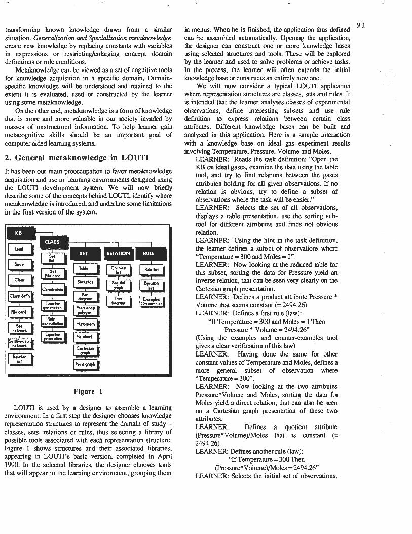
transfonning known knowledge drawn from a similar situation. Generalization and Specialization metaknow/edge create new knowledge by replacing constants with variables in expressions or restricting/enlarging concept domain definitions or rule conditions.

Metaknowledge can be viewed as a set of cognitive tools for knowledge acquisition in a specific domain. Domain­specific knowledge will be understood and retained to the extent it is evaluated, used or constructed by the learner using some metaknow ledge.

On the other end, metaknowledge is a fonn of knowledge that is more and more valuable in our society invaded by masses of unstructured infonnation. To help learner gain metacognitive skills should be an important goal of computer aided learning systems.

2. General metaknowledge in LOUTI

It has been our main preoccupation to favor metaknowledge acquisition and use in learning environments designed using the LOUTI development system. We will now briefly describe some of the concepts behind LOUT!, identify where metaknowledge is introduced, and underline some limitations in the first version of the system.

Figure 1

LOUT! is used by a designer to assemble a learning environment. In a first step the designer chooses knowledge representation structures to represent the domain of study -classes, sets, relations or rules, thus selecting a library of possible tools associated with each representation structure. Figure 1 shows structures and their associated libraries, appearing in LOUTI's basic version, completed in April 1990. In the selected libraries, the designer chooses tools that will appear in the learning environment, grouping them

91 in menus. When he is finished. the application thus defined can be assembled automatically. Opening the application, the designer can construct one or more knowledge bases using selected structures and tools. These will be explored by the learner and used to solve problems or achieve tasks. In the process, the learner will often extends the initial knowledge base or constructs an entirely new one.

We will now consider a typical LOUT! application where representation structures are classes, sets and rules. It is intended that the learner analyses classes of experimental observations, define interesting subsets and use rule definition to express relations between certain class attributes. Different knowledge bases can be built and analyzed in this application. Here is a sample interaction with a knowledge base on ideal gas experiment results involving Temperature, Pressure, Volume and Moles.

LEARNER: Reads the task definition: "Open the KB on ideal gases, examine the data using the table tool, and try to find relations between the gases attributes holding for all given observations. If no relation is obvious, try to define a subset of observations where the task will be easier." LEARNER: Selects the set of all observations, displays a table presentation, use the sorting sub­tool for different attributes and finds not obvious relation. LEARNER: Using the hint in the task definition, the learner defines a subset of observations where "Temperature= 300 and Moles= 1 ". LEARNER: Now looking at the reduced table for this subset, sorting the data for Pressure yield an inverse relation, that can be seen very clearly on the Cartesian graph presentation. LEARNER: Defines a product attribute Pressure * Volume that seems constant(= 2494.26) LEARNER: Defines a first rule (law):

"If Temperature= 300 and Moles = 1 Then Pressure* Volume= 2494.26"

(Using the examples and counter-examples tool gives a clear verification of this law) LEARNER: Having done the same for other constant values of Temperature and Moles, defines a more general subset of observation where "Temperature= 300". LEARNER: Now looking at the two attributes Pressure*Volume and Moles, sorting the data for Moles yield a direct relation, that can also be seen on a Cartesian graph presentation of these two attributes. LEARNER: Defines a quotient attribute (Pressure*Volume)/Moles that is constant (= 2494.26) LEARNER: Defines another rule (law):

"If Temperature= 300 Then (Pressure*Volume)/Moles = 2494.26"

LEARNER: Selects the initial set of observations,

92

I

displays a table presentation of the last defined attribute and Temperature; sorting on Temperature yields another direct relation.

LEARNER: Defines a rule (law) holding for all the observations given initially in the KB: "Ift Then (Pressure*Volume)/(Moles*Temperature) =

8.3142 The striking thing in the preceding example is that it is a

monologue, not a dialogue. This is characteristic of open learning environments. The learner directs the action, sometimes aided by a human teacher who suggests methods and tools, getting ideas for future action from the system's reaction. The system's role is to table, to sort, to graph, to accept set and rule definition, to adapt its presentation tools to newly selected set or rule, to give a clear presentation of a rule's examples and counter-examples for verification by the learner.

This is possible in the basic version of LOUT!, because tools embody general metaknowledge about knowledge processing in the same way a text editor embodies general metaknowledge about text processing. A text editor knows that reordering sentences or paragraphs, searching and replacing words, indenting paragraphs or changing character style, are important to good communication in any particular knowledge domain. In a similar way, a LOUT! application adjusts its subsets inclusion network after set definition (figure 2A), adjusts tables and graphs to set selection (figure 2B), facilitate sorting operations and rule counter-examples display (figure 2C).

A

B

[J&JReal•QIMS] ..,,,, "" PllV T•llp"300

3 [ Temp,..400 ] .~,~ 4000 ",,.. 3500

(19[ nmp,,soos.M01u .. 1 J 3000 2500 . 2000 • F....... M.1- PO\/ P'"II M 1500 • 1000

CU 0.2 ~9US2 2494,:aj; 500 • P2 OJ 1247.11 :NH.al 0 Clt4 o., 1247.IS -21 0.3l.3J . <IO.:D.OO. ll.11>.II 1 1 02 O.'IS 1a10.~ .. -~ Ill , 2+N.26 2"421 ca , 24M.2& :aftil3

IF Tempereture(x) ~ O tll.-THEN P*Y/M • 2496.24 Azat•

,.,,,_iMI 4SO --------Chlanr• d'h\,d 250

MhydrilM sulf 400 StiliM 350

Figure 2

Mo lH

P•YIM 332:1.68 2909.97 3741 .3' 2078.55 3325.68 2909.97

There are however, problems in using tools that are as general as these. It is not certain at all that the average student will be able to achieve anything near the ideal method presented above. In fact, in the first implementation of this learning environment, the designer has been forced to write a detailed activity guide to make sure that the learner proceeds in the right direction.

Decomposing the learning process in a "guided tour" way is contradictory to the very idea of a constructivist learning

strategy. It leads to impoverishment of the problem-solving process, preventing the learner to plan the use of induction tools and methods by himself

The problem here is this: in a complex learning task, the number of necessary operations using general tools grows exponentially. To prevent this without guiding closely the learner, the LOUT! workbench must be enriched with new tools that are concrete representation of more specific metaknowledge.

A first set of such tools have been developed with the SONODOSE project, a physiotherapy training environment on ultra-sound treatment [Paquette 90). Specialized tools have been constructed to help the learner build a consistent, complete and non-redundant set of rule for ultra-sound treatment identification. Evaluation metaknowledge has been embedded in tools to help uncover contradictions between rules, compare the extension of two rules and assess a rule­group's completeness. These tools are not as general as LOUTI's base version tools, but they are useful whenever the generic task of rule construction must be undertaken.

To generalize this approach, we have since then developed new set of tools for two other generic tasks: taxonomy definition and quantitative law induction. The later will now be discussed in some detail, keeping in mind to help a learner solve similar induction problems to the Ideal Gas law.

3. Law induction metaknowledge

In law induction tasks, fundamental AI machine learning research [Langley 87) has demonstrated the importance of combinatorial metaknowledge. In the work of Langley and al. on scientific discovery, induction of quantitative laws is seen as a problem-solving process in a state-operator space. The initial state is a list of expressions that are variables over some domain. Operators can restrict, enlarge the domain or construct more complex expressions. They are applied until a final state is reached where an expression is a constant or a linear expression over a sufficiently large domain, or no more operators can be applied.

The search through the induction problem space is guided by combinatorial metaknowledge. Based on our observation of human problem solvers, using part of Langley's BACON programs heuristics, we have retained the following operators or metaknowledge:

TO INDUCE: (1) Restrict the domain so that all variables

are kept constant, except two called X and Y, and make a first expression list X, Y on this domain.

(2) If X and Y are inversely proportional, add the expression X*Y to the list.

(3) If X and Y are directly proportional, add the expression X/Y to the list

(4) If the last expression F(X,Y) is constant

or a linear function of X and Y, remove X and Y from the expression list

(5) If the last expression F(X,Y) is constant or a linear function of X and Y, stop or enlarge the domain by freeing one variable not in F(X,Y).

Using these operators, the direct induction path to the Ideal Gas law presented in the preceding section, can be summarized as follows:

Abbroviotlons : lnttt.lin•lo: T,H,P,Y ... o T: t.,,..,.1tw•; P: p,-euw•; ,t,i,p",jt19 (1) : T,H,P,Y enrf•!~l'RiilJ Y: vo1'mf.; M: mo,.s; l,jlpJ\ltl9(2): T, H,~,!!IZJ ... T-:soolJ'tal 0 : Qlollol Ml.,, ol>1..-v•tlons: At>l'",ltlt (4): T, H, OIi T•:soolJ'tal T-300 : -I of 0 At>l' ... tl9(5): T,H,PO\I ... ~

Yillll-•tur.•300 Alop",jt19(J): T, H, PO\l ,l!?llB) OIi T•300 T~I: l,jlp",jtl9(4): T,~ Ollra:500 ...... ,.,o ,t,i,p ... t19(5): T, P0\1/H •W -~---:soo """"""" (!): ;~iAn-l!!2ZH!ll • 0 IMrMIK• 1 Aw ...... (4): ... o

Figure 3

Metaknowledge in these operators is generic. With similar heuristics, the BACON programs are able to discover most quantitative laws of elementary physic and chemistry such as Snell's refraction law, Ohm's electricity law or Kepler's third gravitational law. Furthermore, these heuristics were derived from close study of the writings of scientists involved in these laws' first discovery. So it seems a sound pedagogical idea to include them in some way in a new set of LOUTI tools.

4. Law induction metaknowledge in tools

Our implementation of the above operators has led to four new LOUTI tools: • Variable Selection displays, for any selected set, a list

of attribute couples, each being in inverse or direct proportional relation, to help the learner apply operators (1) & (5). (see Figure 4 A, B)

• Construction displays a sorted table of the selected set, with a column for the two initial variables and subsequent expressions constructed using operators; as shown on figure 4C, operators (2) Product, (3) Quotient and (4) Reduce can be applied to the current expression list using options of the private menu.

• Operation Selection counsels the learner on the operation to use on two attributes he selects.

• Constant and Linear Testing computes if an expression is a constant or linear relation, considering an error factor specified by the learner.

R .... t•a, 1able ~ele1 t1on

r:Jl:III for thl Mt ~ l-QIMS, 36 obMrv1tto111, ll.::.t there •r• ne lnterNttncJ couplN ohttrlbulN.

...._ ____ -t r;:;;-'\ Define 11ublet by Mttt119 all v1r11bl11 constantl l::J except tw.

C IDill Construction II Product nom PrH- Yolum. Quotient o1o""• 4·-1 :io 49.88:52 Reduce 1 · • PhosphN 100 24.9426 Bromuna,.,,,a 100 24.9426 Clear cv ....... d,.,,,• 100 24.9426 Size F-..... d,,,,,. 100 24.9426 ---..-p..,,...,. ••• 100 24.9426

Volume

..... • ><"- 100 24.9426 -~~~~---. NiM 100 24 .9426 m 11D --- - -- -~Hum 100 24.9426 Pr-ure

Figure 4

Using these new tools, the Ideal Gas law induction is more easily achieved, the learner proceeding as follows:

LEARNER: Reads the task definition: "Open the KB on ideal gases, examine the data using the table tool, and try to find relations between the gases attributes holding for all given gases". LEARNER: Calls the Variable Selection tool with the set of all observations selected. SYSTEM: Suggest the definition of a restricted subset (Figure 4A). LEARNER: Defines the Temp=300&Moles= 1 subset and calls again the Variable Selection tool. SYSTEM: Suggest a relation between the variables Pressure and Volume (Figure4B). LEARNER: Calls the Construction tool; the sorted table and the associate Cartesian graph clearly show an inverse proportional relationship (Figure 4C). LEARNER: Calls the Operation Selection tool SYSTEM: Suggest to consider a product of the two variables. LEARNER: Selects the product option in the Expression Construction tool; the table and graphics adjust, showing a constant product expression (= 2494.26), verified to a very low precision interval using the Constant Testing tool. LEARNER: Uses the "Reduce" option of the Construction tool, keeping expression T, Mand P*V LEARNER: Defines a more general subset of observation where ''Temperature = 300" and call the Variable Selection tool. SYSTEM: Suggest to consider a relation between the variables Moles and P*V. LEARNER: Calls the Construction tool; the sorted table for the subset and the associate Cartesian graph clearly show a direct proportional relationship between Moles and P*V.

93

94

' ·i

I I

LEARNER: Selects the quotient option in the Construction tool; the table and graphic adjust, showing a constant P*V/M expression (= 2494.26) that can be verified using the Constant testing tool. LEARNER: Uses the "Reduce" option in the Construction tool, keeping expression T and P*V /M for future constructions. LEARNER: Select the initial "Real Gases" observation set. LEARNER: Calls the Construction tool; the sorted table and the associate Cartesian graph clearly show a direct proportional relationship between T and P*V/M. LEARNER: Selects the quotient option in the Construction tool; the table and graphic adjust, showing a constant P*V/M*T expression(= 8.3142), yielding the Ideal Gas Law definition. LEARNER: Defines a rule (law) holding for all the observations given initially in the KB: "If t Then (Pressure*Volume)/(Moles*Temperature) =

8.3142

Comparing this procedure and the one in section 2, one can see that the new set of tool reflects more directly induction heuristics. The learner is freed from most technical operations so he can concentrate on finding a solution path. Further more, such tools are constant reminders of productive induction methods.

Though the learner retains initiative, the system is more active, giving advice at the student request on interesting variable, adequate operations and constancy or linear relationships. While using the tools, the learner has to ask himself good questions about the method.

The end of the preceding dialog suggests that the learner has come to associate "inverse proportional relation" with a product operation, and "direct proportional relation" wi~ a quotient operation, so doesn't need to use the Operauon Selection tool. When the learner comes to find some tool useless, and yet use its effect to choose other actions, we can suppose he has internalize the corresponding metaknowledge. Then, a very important didactic goal has been achieved.

S. Implementing Generic Tools in the LOUTI system

In the LOUTI system, tools are PRISME1 objects inheriting attributes and methods from parent tools or basic interface objects. To add a new tool, it is useful to start with one or more general tools already in the system and to modify their methods.

1 PRISME [Bergeron 88, Nadeau 91] is a programming system of the LISP family with object-oriented and logic programming extensions, fully integrated with one another and with the Macintosh graphic user interface.

Operational tools

We define tools as operational, when they participate in a learner's constructive action. They facilitate action, in our case, applying operators in the problem-space.

For example, the Construction tool is implemented as a descendant of both the Table Tool and the Cartesian Graph Tool, but almost every method had to be rewritten. Activation and deactivation methods needed to be redefine, to achieve coordinate appearance or disappearance of the sorted table and its associated graphs.

The tool's private menu has been profoundly modified to make the Product, Quotient and Reduce options available. These three options achieve several knowledge base operations in a single step: - call attribute definition or destruction operations, - specificy attribute type and computation mode, - construct new product or quotient attribute, - add a column in the sorted table and draw new graphs.

Counseling tools

Unlike operational tools, counseling tools give methodological advice to the learner. They are implemented as descendants of a parent tool having two basic methods:

• evaluating a set of conditions based on indicators to be computed by each counseling tool; • displaying a message based on the conditions met by the learner's knowledge base in its present state.

A particular counseling tool like Variable Selection will compute indicators for direct or inverse proportional relationship for each pair of attributes, for all elements in the selected set of observations. It will display a message accordingly. If there is no such relationship, it will suggest the learner to apply operator (1). If, on the contrary there is one, it will list couples of interesting attributes to consider.

Such counseling tools do not take action on behalf of the learner. Like any other tool in the environment, a counseling tool is used by the learner whenever he feels he needs it Getting an advice leaves a lot of work to do. There are still many paths the learner can take. If fact, counseling tools act like a first-line specialized teaching agent The learner mentally raises his hand and gets a specialized counsel from the agent.

Generic tools

Both operational and counseling tools are domain independent. This opens the possibility to add them to LOUTI' s libraries. They then become available to build any application in which they can be useful. These. ~e knowledge domains where there is at least a class contrumng a certain number of numeric attributes on which subsets, can be defined and numerical relations searched for.

The law induction tools are domain independent but they display messages, tables, graphs or other presentations using domain specific terms. For example, figure 5 shows displays

from the Variable Selection tool and the Construction tool, in a completely different domain from the Ideal Gas law: solar astronomy. Thirty-nine celestial objects are includes in the knowledge base and described by more than thirty attributes, most of which are numeric. It is then possible to use the Law induction tools to induce, for example, Kepler's third gravitational law.

• •••I [39 )Ctlest11l-obtec

.... 'I ' [l:sl for the Nt P1111tll, 9 obHr,1t10111, ~ the foll wt 119 couples of 1ttrlbutes 1r11nt1restt119:

( rtwlutlon dtst1nce) (me,s onv1ty) ~ (orbft1l-1peed dt1t1nce) (orbital-speed revolution)

(11bent1on-speed orwttv) Cl1bent1on-speed me,,)

10!!1 Construction 11111 Product - rivollltlon dist..- Quotient dt1t1nct • moroun,i 68 !1.7~7 v- 22S 1.081...00S Reduce ~ 3'5 2.496e+008 Cleer • mars 687 2.27~ Size • ,M>ltH' 4331 7.793.+oo8

3 • ··""' 107S2 1.427.+009 ,-.:• •• I ......... 30684 2.869-+009 I I I I I

Mjltun. 60266 4.so.+DM pluton 90520 :1.,-+009 revolution

Figure S

This induction problem-space is quite different from the ideal gas law problem. Kepler's third law contains only two variables instead of four, but the relation between them is more complex. To construct the expression D3/R2 = est, one does not need to restrict or enlarge the observation set, but to apply the product and quotient operators many times on expressions obtained by previous application of the same operators.

The fact that a law such as this one can also be derived using the same induction tools shows their generic character. But certainly they are not general tools, useful in any induction problem. Adding new operators would enable induction of more complex quantitative laws, but for ill­structured problem domains such as quasi-laws in economics or foreign policy, combinatorial metaknowledge such as the one presented here would prove its limit. For such domains, rule construction metaknowledge such as we have embedded in the physiotherapy environment might provide a better start.

This discussion underlines our general approach: to find classes of similar problems where useful metaknowledge can be identify, to embed this metaknowledge both in operational tools and counseling tools, and to make these tools available to the learner in the learning environment

6. Learner Guidance in Open Learning Environments

We have presented an approach to the problem of guidance in open learning environments. Especially when problems are difficult, it is necessary for the system to provide some sort of advice, without restraining the necessary liberty involved in real problem-solving activities. We will now discuss this approach more in detail, within the framework

of Intelligent Tutoring Systems (ITS) research.

The learner as a knowledge engineer

The following quotation from John Self expresses well the foundation of our approach:

"An ITS philosophy (of Knowledge transmission) runs counter to almost everything of significance in twentieth century educational philosophy. All the major figures (Dewey, Montessori, Piaget, Rodgers, even Skinner) have rejected the "education as transmission" model, which had dominated the previous three centuries in favor of an "education as growth" model. Knowledge is not the kind of commodity which can be transmitted. It cannot be simply received by students but must be constructed anew by them. While most ITS researchers declare such a view, it is belied by the systems we build." [Self90]

We hope we are not! In fact, in our learning environments, the student's activity is essentially knowledge construction. The learner's explores the knowledge freely using presentation tools in the application. Then, a task or a problem makes him explore knowledge in a more structured way. Finally he will write down a conjecture, test it and modify it if necessary to increase its predictive power.

Many works in ITS have considered the analogy between the learner's construction activity and knowledge engineering. For example, William Clancey proposes the following approach:

"by studying and modeling the work of the knowledge engineer, we should be able to build models of the learning process that can be integrated in the design of an Intelligent Tutoring System." [Clancey 88]

While Clancey here looks at the knowledge engineer as a learner to model, we essentially see the learner as a knowledge engineer. In both cases, the study of knowledge engineering is interesting because it helps identify more clearly useful metaknowledge. Since knowledge engineering by the student is not and easy task we seek to make metaknowledge available in the form of interactive tools included in the learning environment.

Metaknowledge in tools and heuristic guidance

We are certainly not the first to investigate the use of metaknowledge in learning environments. Clancey has used metaknowledge classified as support, structural and strategic knowledge and used in his systems for medical training [Clancey 83]. Vivet has integrated the mathematician metaknowledge in an expert-system solving symbolic integration problems, that can be used for tutoring a student on those tasks [Vivet 84].

In open environments, Papert's microworld approach [Papert 80] puts great emphasis on the use of problem­solving metaknowledge through LOGO programming.

95

9 6 Learning environments such as SMITHTOWN [Shute 86), REFRACT [Reimann 88] and VOLTAVILLE [Glaser 88], built at Pittsburgh's LRDC have a strong metacognition emphasis.

In our view, metaknowledge should be introduced explicitly in learning environments to help the student gain and use domain independent methodological knowledge. This idea is supported by a systematic study of the use of LOGO problem-solving in classrooms [Swan 89). This study shows that LOGO programming, though having an effect on problem-solving skills, is not significantly better without explicit teaching of problem-solving methods such as problem decomposition, forward-chaining or analogy. Both are necessary for metaknowledge use and acquisition.

In a similar way, we hypothesize that the use by the learner of operational tools embedding metaknowledge, and the use of counseling tools, also based on metaknow ledge, are both necessary to help the student achieve knowledge construction tasks.

Operational tools enable activity similar to LOGO program construction, with its programming-evaluating­debugging cycle. Using operators on the knowledge base, the learner construct a problem solution by a similar "knowledge debugging" process.

On the other hand, counseling tools are a constant reminder of evaluation, utiliz.ation and creation metaknowledge, in other words: problem-solving methods. They provide an interactive initiation to problem-solving methods, a form of heuristic teaching first proposed by George Polya [Polya 57, 67) . In this way, in a very open learning environment and task, it is possible to offer methodological guidance that should constrain the leranrer's construction process towards productive results.

Generic metaknowledge

A last aspect of the question is the generality or scope of metaknowledge. In their synthesis on induction, Holland and al. underline:

"General methods such as means-ends analysis are not sufficient to explain problem-solving skills. Human expertise lies, in a critical way, on specialized methods and a good representation of knowledge in the considered domain" [Holland 87]

In their work on scientific discovery, Langley and al., also consider a hierarchy of heuristics ( or metaknowledge) from general weak methods, to more specialized strong methods:

"We can picture a hierarchy of heuristics, with the top levels consisting of very general algorithms that require little information about the task domain to which they are applied and are correspondingly applicable to a great many domains. As we proceed downward in the hierarchy of heuristics, we make more and more demands on information about the task domain,

and there are correspondingly fewer domains to which the heuristics apply ( ... ). Since the more general heuristics operate on the basis of less information, we may expect them to be less selective, and hence less powerful, than heuristics that make more use of information about the task structure. Hence, general heuristics are weak methods, while task-specific heuristics, such as our procedure for solving algebra equations, may be strong methods. The less structured a problem­solving task is, the less information one can draw upon construct strong heuristics." [Langley 87)

Reviewing recent ITS literature shows that the vast majority of projects have concentrated on strong, domain­specific methods, consistent with a guided discovery approach. Metaknowledge has been used mainly in the tutorial module to achieve close domain-dependant learner's guidance. At the opposite, micro-world and learning environment projects are characterized by the use of weak methods, most of the time without any guidance from the system.

Our work is an attempt to reconcile these approaches. We have first represented weak methods in quite general tools, in the basic version of the LOUTI system, in a typical "micro-world spirit". Then, we have concentrated on the introduction of more specific metaknowledge and stronger methods for generic tasks like rule construction, and law induction.

We can define our research program as this: to seek structured tasks where powerful, while largely domain­independent methods can be represented in tools to support a learner-centered construction activity.

It is hoped that with these tools, a learner can experiment fruitful knowledge construction activities across different fields of knowledge.

Acknowledgements

The author wishes to underline the contribution of Anne Bergeron, Jacques Bordier, Charles Camirand, Serge Carrier, Annick Hernandez, Martin Longpre and Renaud Nadeau to the LOUTI project, and the support of the APO-Quebec

. Center and Tele-universite.

References

[Anderson 80) J. Anderson. Cognitive Psychology and its implications. Freeman and Co., 1980

[Bergeron 88) Bergeron A., Bouchard L., Nadeau R., A Mu/ti-Paradigm Development System for Exploratory Environments, CSCSI 88 Proceedings, Edmonton,1988.

[Bergeron 90) Bergeron, A. and Paquette, G. Discovery Environments and Intelligent Learning Tools, in Intelligent tutoring systems: at the crossroad of Artificial Intelligence and Education (Eds C. Frasson and G. Gauthier), Ablex Publishing, Norwood NJ.

[Bordier 90] J. Bordier, G. Paquette and S. Carrier, Building Learning Environment using Generic Software, Proceedings of the 4th World Conference on Computers and Education, Sydney, Australia, July 1990.

[Clancey 83] W. J. Clancey. The Epistemology of a Rule­Based Expert Systems. Artificial Intelligence 20, pp 163-210, 1983.

[Clancey 88] W. J. Clancey. The Knowledge Engineer as Student: Metacognitive Bases for Asking Good Questions, in Learning Issues for Intelligent Tutoring Systems, H. Mandi & A. Lesgold (Eds), Springer-Verlag, 1988.

[Glaser 88] R. Glaser, K. Raghavan and L. Shauble.Voltaville, a Discovery Environment to Explore the Laws of DC Circuits. Proceedings of the ITS-88 conference, Montreal, June 1988.

[Holland 87] J.H. Holland, K.J. Holyoak, R.E. Nisbett, P.R. Thagard. Induction, Processes of Inference, Learning, and Discovery, MIT Press, Cambridge, 1987.

[Langley 87] P. Langley, H.A Simon, G.L. Bradshaw, J.M. Zytkow, Scientific Discovery, Computational Explorations of the Creative Processes, MIT

[Minsky 88] M. Minsky. Society of Mind, MIT PRESS, 1987.

[Nadeau 91] R. Nadeau. Integration de trois paradigmes de programmation, Memoire de maitrise en mathematique and informatique, UQAM, 1991.

[Papert 80] S. Papert. Mindstorm: Children, Computers andPowerfulideas, Basic Books, 1980.

[Paquette 88a] G. Paquette. Environnements d'apprentissage a base de connaissances. Conference invitee au collogue international de pedagogie informatique, Actes publies par l'Universite de Bologne, Italie, juin 88.

[Paquette 88b] G. Paquette. Le developpement d'outils intelligents d'apprentissage pour le traitement des connaissances. Actes de ITS-88, U. de Montreal, June 1988.

[Paquette 90] G. Paquette, R. Nadeau and M. Longpre. A support-system for Knowledge Engineering by the Student, CSCSI-90, Ottawa, may 1990.

[Paquette 91] G. Paquette, Le role des metaconnaissances dans LOUT/, un generateur d' environnement cf apprentissage, Actes du collogue KMET'90, IOS Press, Amsterdam, avril 1991.

[Pitrat 90] J. Pitrat. Metaconnaissance, avenir de l' intelligence artificielle, Hermes, Paris, 1990.

[Polya 57] George Polya. How to Solve It?, Princeton University Press, 1957.

[Polya 67] George Polya La decouverte des mathematiques, Wiley, Dunod Paris, 1967.

[Popper 61] K.R. Popper, The logic of scientific discovery, Science editions, 1961.

[Reimann 88] P. Reimann, Modeling discovery learning processes in a microworld for optics, European summer university on intelligent tutoring systems, Universite du Maine, Le Mans, 1988.

[Self 90 J. Self. Theorietical Foundations of Intelligent Tutoring Systems Journal of Artificial Intelligence in Education, AACE, Phoenix Arizona, vol 1-4, summer 1990.

[Shute 86] V.J. Shute and J.G. Bonar. An intelligent tutoring system for scientific inquiry skills. Proceedings of the Eighth Cognitive Science Society Conference, Amherst, Massachusetts, 1986.

[Swan 89] Karen Swan, Logo Programming and the Teaching and Learning of Problem Solving, Journal of Artificial Intelligence in Education, AACE, Phoenix Arizona, fall 1989.

[Vivet 84] M.Vivet. Expertise mathematique and informatique: CAMEUA, un logiciel pour raisonner and calculer. These d'etat, Universite de Paris VI, 1984.

[Wenger 87] Etienne Wenger, Artificial Intelligence and Tutoring Systems, Computational and Cognitive Approaches to the Communication of Knowledge, Morgan Kaufman, Los Altos, USA, 1987.

97

98

I

I

Computing The Lower Bounded Composite Hypothesis By Belief Updating

Yang Xiang Expert Systems Laboratory Centre for Systems Science

Simon Fraser University Burnaby, B.C., Canada, V5A 1S6

yangx@cs.sfu.ca

Abstract When making a decision under uncertainty, we often impose a threshold on the expected util­ity. Such a threshold dictates a lower bound for the posterior probablity of the compos­ite hypothesis on which the decision is based. This paper introduces the concept of Lower Bounded Composite Hypothesis (LBCH) . A LBCH is also a Most Likely Composite Hypoth­esis (MLCH) if the lower bound is greater than 0.5. The paper presents a threshold method for computing LBCHs by belief updating (the com­putation of Posterior Marginal Distributions (PMDs)) in Bayesian networks. There has been no known algorithm computing MLCHs in clique tree based secondary structures of Bayesian networks. The method presented al­lows the computation of LBCHs in such struc­tures using existing belief updating algorithms. The method is practical only for computing LBCHs over a small number of (about 20) variables. However, the networks can contain an arbitrarily large number of variables. It is argued that restricting the computation of LBCHs to a small number of variables can often be desirable. An example is given to illustrate the method.

1 Introduction Bayesian belief networks combine graphic representation of causal domain models and probability theory. Over the last decade, they have gained increasing popularity as a natural, efficient knowledge representation method and a consistent inference formalism for building knowl­edge based systems which require reasoning under un­certainty.

Bayesian networks have been termed in the literature belief networks, causal networks, or causal probabilistic networks. Formally a Bayesian network [Pearl 88] is a triplet (N, E, P).

• The domain N is a set of nodes each of which is la­beled with a random variable. Each variable has a set of mutually exclusive and exhaustive outcomes

which forms its space. 'Node' and 'variable' are used interchangeably in the context of Bayesian nets. A joint assignment of outcomes for a set of variables X = { A1, ... , An} ~ N is denoted by the concate­nation of corresponding outcomes x = a1 ••• an,

• E is a set of arcs such that (N, E) is a directed acyclic graph. The arcs signify the existence of direct causal influences between the linked vari­ables. Causality is directed along the directed arcs. The basic dependency assumption embedded in Bayesian nets is that a variable is independent of its non-descendants given its parents.

• Pis a joint probability distribution quantifying the strengths of the causal influences signified by the arcs. P specifies for each Ai E N the distribution of the random variable labeled at Ai conditioned by the values of Ai's parents 11'i in the form of a conditional probability table p(A;l1ri)· p(A; j1ri) is a normalized function mapping the joint space of {Ai} U 11'i to (0, 1]. The joint probability distribu­tion P can be represented as P = p( A1, ... , Aa) = Ilf=1 p(Ai j1r;).

Inference in Bayesian networks can provide answers to essentially two types of queries. The first type asks the PMDs in the form: p(Ale) where A is a single vari­able and e stands for all the evidence acquired so far. Computing PMDs is termed belief updating (Pearl 88]. A PMD allows one to rank the set of possible outcomes for variable A according to their credibility given e, for example, whether a patient has a particular disease or not; or whether a component in a machine is faulty.

The second type asks the MLCH. Let X ~ N be a set of variables. One computes a joint assignment x of outcomes to all variables in X such that

('v'x')p( x le) > p(x' le).

A joint assignment x ' is called an instantiation of X, or a composite hypothesis, or a configuration, or an ex­planation. Computing the MLCH is termed belief revi­sion (Pearl 88]. The MLCH is needed when one tries to determine the exact state of the world (when X = N ) (Poole and Provan 90], for example, to give a description of the overall status of a patient.

In the literature, the two types of inference have been considered distinct. Consider two variables A and B.

The computation for PMDs may indicate that a1 is the most likely outcome of A and b1 is the most likely out­come of B. While the MLCH for X = {A,B} may turn out to be a1 b2 (Pearl 88, Poole and Provan 90]. This paper shows when this is not the case. Based on the distinct nature of the two inference types, separate algo­rithms have been developed for each type of inference. For computation of exact PMDs, there are A - 1r mes­sage passing in trees (Pearl 86], arc-reversal and node­removal [Shachter 86, Shachter 88], directed clique tree message passing (Lauritzen and Spiegelhalter 88], junc­tion trees of cliques (Jensen, Lauritzen and Olesen 90a, Jensen, Olesen and Andersen 90b], multiply sectioned Bayesian networks and junction forests of cliques [Xiang, Poole and Beddoes 91]. For computation of ap­proximate PMDs, there are logic sampling (Henrion 88], and clamped logical sampling (Pearl 88]. For compu­tation of the MLCH, there are message passing, cutset conditioning, clustering [Pearl 88] as exact methods; and TopN [Henrion 91] as an approximate method.

This paper studies the relation between the two types of inference. In particular, the paper presents the fol­lowing. (1) The notion of Lower bounded Composite Hy­pothesis (LBCH) is introduced from a decision theoretic context. LBCHs are MLCHs when the lower bound is greater than 0.5. (2) It is shown that LBCHs can be obtained by belief updating. (3) Although computation of LBCHs by belief updating is directly applicable to hypothesis sets of less than about 20 variables, it is ar­gued that not only this is often sufficient with respect to one's current attention, but this is often desirable com­pared to computing a MLCH over all domain variables. (4) There is no known algorithm computing MLCHs in clique tree based secondary structures of Bayesian net­works. By establishing the relation between belief up­dating and revision, one can extract extra information (LBCHs) beyond PMDs from the secondary structures in a straightforward way.

Section 2 introduces the LBCH notion from maxi­mum expected utility principle of decision theory. Sec­tion 3 and 4 presents the threshold method for com­puting LBCHs by belief updating. Section 6 discusses the application of the method for inference in secondary structures. Section 7 demonstrates the method by an example. Section 8 summarizes the main results of the paper.

2 Lower Bounded Composite Hypotheses

Decision theory argues a rational decision maker should act according to Maximum Expected Utility (MEU) principle (von Neumann and Morgenstern 47]. Following the formulation in (Andreassen et al. 89], the decision maker's preference can be represented by a util­ity function U(x; lxi) where x; and Xj are both composite hypothesis on a set X of variables. The function spec­ifies the utility of action based on Xi given that xi is true. We consider reward/ penalty type of utility func­tions. The utility of a correct decision (i = j) is pos­itive (reward). The utility of at least one wrong deci-

sion (i # j) is negative (penalty) . Utility functions in many applications belong to this type. Military actions on battlefields are such examples. In medical diagnoses, treatments ( medication, surgery) based on wrong diag­noses can cause side effects and inappropriate follow-ups, can prolong and worsen the patients' suffering due to the untreated real disease. There has been argument [Huchlenbroich 91] that medical expert systems should base their conclusion on "conclusive" evidence to avoid incorrect diagnosis as much as possible.

The MEU principle says that given evidence e, and utility function U, one should choose the action indicated by Xi which has maximal expected utility:

Denote the reward/ penalty type utility as the follow­ing.

i = j i#j

where min(wj) = - W, and V, W are positive. The expected utility for Xi is

> Vp(x; le) - W(l - p(x; le)) = W(l + r)(p(x; le) - p') (1)

where r = V/ W (reward/penalty ratio) and p' = 1/ (1 + r ).

When making a decision under uncertainty, we often impose a threshold U0 on the expected utility. If MEU is less than U0 , we would delay the decision and try to gather more information until MEU is greater than U0 •

The following definition gives one such threshold.

Definition 1 With a reward/penalty type utility, a com­posite hypothesis xis profitable if and only if U(x) > 0.

By equation 1, if p(xi le) > p' , then x; is profitable. Consider an extreme case of the reward/ penalty ratio in equation 1. If V < < W , then p' -+ 1. A profitable composite hypothesis Xi has to satisfy p(x;le) -+ 1. In this case, trying to find the profitable composite hypoth­esis means trying to avoid heavy penalty. For instance, when a medication can cure a patient if he has the disease but can kill him if the diagnosis is wrong, the physician should be very careful to ascertain the diagnosis. We see that p' is a belief threshold which results from the expected utility threshold 0.

Zero is not the only possible utility threshold. Con­sider another extreme case of the reward/ penalty ratio in equation 1. if V >> W , then p' -+ 0 and the right side of the equation is approximately Vp(xi le). In such case, many composite hypotheses are profitable but the reward associated may be very low compared to V. If one sets minimum expected reward Vo, then one should try to find Xi such that p(xi le) > Vo / V . Again we see a belief threshold Vo / V.

99

I

·1

. I I

100 To summarize, when making a decision under uncer­

tainty, one often has a utility dependent lower bound po such that one needs to find the composite hypothsis Xi

which satisfies p(xile) > Po, In the about two extreme cases, Po takes the values of p' and Vo/V respectively. We call such Xi Lower Bounded Composite Hypothesis (LBCH).

LBCHs may not be unique if p0 ~ 0.5.

Definition 2 A composite hypothesis x is dominant if and only if p(xle) > 0.5.

Proposition 1 A LECH is a MLCH and is unique if it is dominant.

Since dominant LBCHs are profitable, unique and most likely, they are more useful than non-dominant LBCHs.

Given a state of knowledge, there may not exist any LBCH relative to a particular po. One can, however, strive for LBCHs lly collecting more evidence to increase the amplitude of p(xile).1

3 Computing LBCHs with Belief Updating

This section derives the condition under which belief up­dating can be used to compute LBCHs.

Consider a set X = A1 ••• An of binary ( this restric­tion will be eliminated latter) variables and an instanti­ation x of X. The following lemma provides a sufficient condition for computing LBCHs.

Lemma 1 Let x = a1 .. . an be an instantiation of a set X of n binary variables. x is a LECH relative to po if p(a; ie) > (n - 1 + Po)/n (i = 1 ... n).

Proof: To simplify the notation, write p(a1 . .. an le) as P1...n,

and p(a1a2 . . . an le) as PI. .. n where the bar means 'not' . Let T = ( n - l + Po) / n.

n

L Pi = (P1.. .n + P12...n + • • • + P12 ... n + i=l ct

n-1

P123 .. . n + ·' ' + P1...n-ln + · '· + P12 .. . n) -...._..,

+ ... + cn-1

n - 1

(P1...n + PI ... n + · · · + P1...n-ln +

· · · + P2 .. . n-1n) ...___ c:::

= n(p1 ... n) +

ci n-1

(n - l)(Pr ... n +.,. + P1...n) + Ct n

(n - 2)(Pu ... n + ... ) + ..._____. c~

1 For simplicity of presentation, we assume the cost of col­lecting evidence is much smaller than V + W .

l(P1...n-ln + • • •) ________.. c:-1

> nT

Since the terms in the parentheses in the second equa­tion are all different, the above implies

P1.. .n > nT - ( n - l) = Po

0

A variable A of multiple values can be transformed into a binary variable A', with the outcome a of A in which one is interested as one outcome of A', and with other outcomes of A congregated as the other outcome of A'. Since such transformation is always possible, Lemma 1 can be generalized to variables other than bi­nary ones.

Lemma 1 establishes a threshold for each p(aile). Once each variable in X has one outcome passing the threshold, the conjunction of this set of outcomes forms a LBCH on X. It can be seen from the above proof that the threshold for each outcome is not necessary. Replac­ing such threshold by a threshold for the sum of p( ai le), one has the slightly stronger result ( (2) in the following theorem).

Theorem 1 Let x = a1 ... an be an instantiation of a set X of n variables. x is a LECH relative to Po if

1. (individual threshold) p(ade) > (n - 1 + p0 )/n (i = 1 .. . n) or

2. (sum threshold) I:7=1 p(a; le) > n - l + Po,

Table 1 shows the threshold for ( 1) in theorem 1 in relation with n when Po = 0.5.

I (n-0~5)/n I 0.~5 3 5 10 20

0.83 0.90 0.95 0.975

Table 1: Threshold for marginal probabilities

4 How Restrictive is the Threshold Method?

Table 1 shows that the computation of LBCH (with Po = 0.5) of more than about 20 variables by belief up­dating requires above 0.975 posterior probability for each outcome involved. This seems to be too tight a restric­tion on the size of the application domain. Fortunately, although the number of variables of an application do­main can easily exceed 20, computation of LBCHs over less than about 20 variables can often be justified and can even be desirable. Since dominant LBCHs are also MLCHs (Proposition 1) and are more useful than non­dominant LBCHs, the following discussion refers ma­jorly to MLCHs to match the concept used in the ref­erenced literature. We specify the conclusion applicable to LBCHs whenever possible.

Figure 1: Illustration of problems with belief revision

4.1 Belief revision. over all variables is not always desirable

The difficulties associated with belief revision over all variables have been identified in [Pearl 88, Poole and Provan 90]. First of all, there is the compu­tational problem. If the MLCH is to cover the entire domain, every piece of evidence must be propagated to the entire network. Unobserved consequence variables no longer block the propagation as is the case in belief updating. For example (Figure 1), if variable C is un­confirmed, the subnetwork NA is independent of NB if PMDs are to be computed. However, in the case of belief revision over all variables, when evidence is available in NA, it has to be propagated to NB in order to find the MLCH. This would impose heavy computational over­head in larger applications.

Secondly, there is the conceptual problem. In belief revision, changing the space where MLCH is computed will change the outcome for each variable. For exam­ple (Figure 1), assuming all evidence is contained in NA, and A, Care uncertain, computing the MLCH in NA or in N may end up with different assignments for variable A. When a diagnosis problem is coupled with a holiday planning, the imagination of the uncertainty of trips can render a highly likely normal diagnosis to become posi­tive (with the disease) as pointed out by Pearl [1988].

It should be emphasized that this conceptual problem is not unique to belief revision in Bayesian networks. Belief revision can be viewed as an optimazation task. Optimization is, in general, sensitive to the space over which some target function is optimized. Belief updat­ing does not suffer from the above conceptual problem because it is not a optimazation task.

The above problems suggest that computation of the MLCH over all variables of the domain is not always desirable.

4.2 Variables which should be covered by a MLCH

In order to overcome the problems associated with be­lief revision over all variables, Pearl [1988] proposed to circumscribe a domain into a set of variables called ex­planation corpus, and to compute the MLCH only over

101 the corpus. According to Pearl, the corpus includes ev­idence and ancestors of evidence variables which have a significant impact on pending decisions. Restricting computation of the MLCH on the corpus will eliminate a substantial number of variables in the domain. In this subsection, we take a closer look at the variables included in the corpus. The purpose is to examine the possibility of focusing the computation to an even smaller set of variables.

Typically a known evidence variable takes one of its outcomes. Therefore, within the corpus, one can fur­ther eliminate the evidence variables from computation of the MLCH. The remaining variables are the ancestors of the evidence variables. These variables can be orga­nized in different levels of abstractions. For example, in medical applications, a Bayesian net can have symp­tom variables as leaves. The successive next higher levels can be biological state level, disease or syndrome level, and disease groups level ( representing diseases with some common characteristics). Not all of them are of a physi­cian's current interest. Usually, only variables at certain level of abstraction is of physician's utmost interest. The number of such variables will be much smaller than the number of variables within the explanation corpus.

When the number of variables in the abstrac­tion level of current attention is large, an im­portant strategy can be applied as suggested in [Patil, Szolovits and Schwartz 82] . One can move up an abstraction level where the important differences are rep­resented by a smaller set of higher level hypotheses. Af­ter gathering further evidence such that the differentia­tion at the higher level is resolved, one can move down to the lower level to differentiate in greater detail. Fo­cusing one's attention in this fashion, one needs only to compute the MLCH on a small number of variables.

The existence of a LBCH over a set of variables is rela­tive to an adequate amount of evidence. Thus it is often useful to know there is no LBCH over a set of variables given the current state of knowledge. The following the­orem gives one condition. Its proof is trivial.

Theorem 2 Let X be a set of n variables. Let A E X have m possible outcomes { a1, ... , am}. If p( a;je) < Po ( i = 1 ... m), then none of the instantiations of X is a LECH relative to Po,

Theorem 2 asserts that there is no LBCH if A is in­volved in the composite hypothesis. That is, given the available evidence, one can not make any strong com­mitment on any composite hypothesis which involves A. Perhaps, one could choose to collect more evidence in order to sharpen the distribution and to make a better informed decision or to make a decision with A ignored. Both can be seen in medical diagnosis. When a doc­tor does not have adequate evidence to give a positive diagnosis on a disease, he/she may either perform more tests on the patient or give no treatment until the disease further manifests.

5 Computation of LBCHs

Computationally, we specify the abstraction level of cur­rent interest in the explanation corpus. To compute

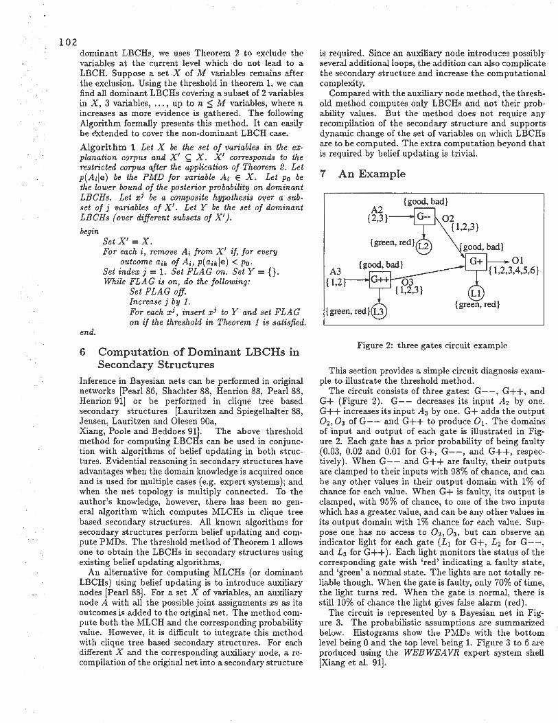
102

. I

· 1

I

dominant LBCHs, we uses Theorem 2 to exclude the variables at the current level which do not lead to a LBCH. Suppose a set X of M variables remains after the exclusion. Using the threshold in theorem 1, we can find all dominant LBCHs covering a subset of 2 variables in X, 3 variables, ... , up to n ~ M variables, where n increases as more evidence is gathered. The following Algorithm formally presents this method. It can easily be extended to cover the non-dominant LBCH case.

Algorithm 1 Let X be the set of variables in the ex­planation corpus and X' ~ X. X' corresponds to the restricted corpus after the application of Theorem 2. Let p(A;le) be the PMD for variable A; E X. Let Po be the lower bound of the posterior probability on dominant LBCHs. Let xi be a composite hypothesis over a sub­set of j variables of X '. Let Y be the set of dominant LBCHs ( over different subsets of X' ).

begin

end.

Set X ' = X. For each i, remove A; from X' if, for every

outcome a;k of A;, p(a;kle) < po. Set index j = 1. Set FLAG on. Set Y = {}. While FLAG is on, do the following:

Set FLAG off. Increase j by 1. For each xi, insert xi to Y and set FLAG on if the threshold in Theorem 1 is satisfied.

6 Computation of Dominant LBCHs in Secondary Structures

Inference in Bayesian nets can be performed in original networks [Pearl 86, Shachter 88, Henrion 88, Pearl 88, Henrion 91] or be performed in clique tree based secondary structures [Lauritzen and Spiegelhalter 88, Jensen, Lauritzen and Olesen 90a, Xiang, Poole and Beddoes 91]. The above threshold method for computing LBCHs can be used in conjunc­tion with algorithms of belief updating in both struc­tures. Evidential reasoning in secondary structures have advantages when the domain knowledge is acquired once and is used for multiple cases ( e.g. expert systems); and when the net topology is multiply connected. To the author's knowledge, however, there has been no gen­eral algorithm which computes MLCHs in clique tree based secondary structures. All known algorithms for secondary structures perform belief updating and com­pute PMDs. The threshold method of Theorem 1 allows one to obtain the LBCHs in secondary structures using existing belief updating algorithms.

An alternative for computing MLCHs ( or dominant LBCHs) using belief updating is to introduce auxiliary nodes [Pearl 88]. For a set X of variables, an auxiliary node A with all the possible joint assignments xs as its outcomes is added to the original net. The method com­pute both the MLCH and the corresponding probability value. However, it is difficult to integrate this method with clique tree based secondary structures. For each different X and the corresponding auxiliary node, a re­compilation of the original net into a secondary structure

is required. Since an auxiliary node introduces possibly several additional loops, the addition can also complicate the secondary structure and increase the computational complexity.

Compared with the auxiliary node method, the thresh­old method computes only LBCHs and not their prob­ability values. But the method does not require any recompilation of the secondary structure and supports dynamic change of the set of variables on which LBCHs are to be computed. The extra computation beyond that is required by belief updating is trivial.

7 An Example

A3 { 1,2

{good.bad}

G-- 02 { 1,2,3}

Figure 2: three gates circuit example

This section provides a simple circuit diagnosis exam­ple to illustrate the threshold method.

The circuit consists of three gates: G--, G++, and G+ (Figure 2). G-- decreases its input A2 by one. G++ increases its input A3 by one. G+ adds the output 02, 03 of G-- and G++ to produce 01. The domains of input and output of each gate is illustrated in Fig­ure 2. Each gate has a prior probability of being faulty (0.03, 0.02 and 0.01 for G+, G--, and G++, respec­tively). When G-- and G++ are faulty, their outputs are clamped to their inputs with 98% of chance, and can be any other values in their output domain with 1 % of chance for each value. When G+ is faulty, its output is clamped, with 95% of chance, to one of the two inputs which has a greater value, and can be any other values in its output domain with 1 % chance for each value. Sup­pose one has no access to 02, 03, but can observe an indicator light for each gate (L1 for G+, L2 for G- - , and L3 for G++ ). Each light monitors the status of the corresponding gate with 'red' indicating a faulty state, and 'green' a normal state. The lights are not totally re­liable though. When the gate is faulty, only 70% of time, the light turns red. When the gate is normal, there is still 10% of chance the light gives false alarm (red).

The circuit is represented by a Bayesian net in Fig­ure 3. The probabilistic assumptions are summarized below. Histograms show the PMDs with the bottom level being O and the top level being 1. Figure 3 to 6 are produced using the WEB WEA VR expert system shell [Xiang et al. 91] .

p(G+ = bad) p(G- - = bad)

p(G ++=bad)

p(A2 = 2)

p(A3 = 1)

p(02 = A2 -1 IA2, G - - = good)

p( 02 = A2IA2, G - - = bad) p(02 ::j:. A2 IA2, G - - = bad)

p(03 = A3 + 1IA3, G ++=good)

p(03 = A3IA3, G ++=bad)

p(03 ::j:. A3IA3, G ++=bad)

= 0.03 = 0.02

= 0.01

= 0.5

= 0.5

= = = =

1

0.98

0.01

1

= 0.98

= 0.01

p( 01 = A2 + A3IA2, A3, G+ = good) = 1

p(Ol = max(A2,A3) IA2,A3,G+ = bad)

p( 02 ::j:. max(A2, A3)IA2, A3, G+ = bad)

p(L = redlG = good)

p(L = redlG = bad)

lnlo A3

= 0.95 = 0.01 = 0.1 = 0.7

Figure 3: Expected behavior of three gates circuit after inputs A2, A3 are specified.

Suppose one knows that the inputs are A2 = A3 = 2. Figure 3 shows sharp distributions for all gates, which represents one's belief that, without any evidence, every­thing is expected to be normal. The expected output of the circuit is 4.

Unfortunately, the output is measured as 6. Entering this evidence into the network, PMDs of both G-- and G+ show the possibilities of fault ( the outcome 'bad' (b) in both gates has a probability value greater than 0.4 in Figure 4). With the understanding of the circuit, one can tell that only two cases are quite likely. One is that G-- is faulty and G+ and G++ are normal. In this case G- - produces output 3 which explains the error. The other is that G+ is faulty and G-- and G++ are normal. In this case G-- produces the expected value 1 and G+ generates the error. Other combinations are quite unlikely. However, without assuming this global

Figure 4: Output 0 1 = 6 rather than expected 4 is ob­served.

Figure 5: The indicator light L2 is found to be red (sig­naling faulty).

knowledge, it is not obvious from the PMDs whether both gates are faulty, or only one of them. Let the lower bound Po = 0.5. Since none of the outcomes of either gate is greater than 0. 75, the threshold by theorem 1, one can not determine the LBCH for this pair of gates. Additional evidence has to be gathered.

After checking the indicator light L2 and entering the value 'red' (signaling faulty), Figure 5 shows p(G- - = badle) = 0.82, p(G+ = goodle) = 0.80, p(G + + = goodle) = 0.99. To determine the LBCH over two vari­ables G-- and G+, this result is sufficient according to the individual threshold of theorem 1. The result is also sufficient for the LBCH over three gate variables ac­cording to the sum threshold of theorem 1 ( the thresh­old is 2.5). But it is not sufficient for the LBCH over three gate variables if the individual threshold of theo­rem 1 is adopted (0.83). Suppose this threshold is used and one gathers another piece of evidence L1 = green

10 3

104

J

I

(Figure 6). One finally has p(G - - = bad!e) = 0 .93 , p( G+ = goodle) = 0.92, and p( G + + = good le) = 0.99, which give the LBCH over three gate variables by any of the two thresholds. Using auxiliary node method for three gates, the LBCH has the probability value 0.92.

Info A3

Figure 6: The indicator light L1 is found to be green ( signaling normal).

8 Conclusion

This paper presents a straightforward threshold method of computing the LBCH via belief updating. The con­cept of LBCH is introduced in a decision theoretic con­text where the decision maker imposes a threshold on the expected utility. Dominant LBCHs are also MLCHs. The concept can equally well be introduced in the con­text where utility functions are non-negative. The se­lected context is felt to be closer to many practical situ­ations.

Although the threshold method is practical only if the number of variables over which the LBCH is computed is small, it is argued that computing the LBCH over small number of variables can often be justified and is often desirable.

The method can be used in conjunction with any belief updating algorithm either based on original networks or based on secondary structures. There has been no known algorithm performing belief revision in clique tree based secondary structures. Such secondary structures have advantages when domain knowledge is acquired once and is used for multiple cases ( e.g. expert systems), and when the net topology is multiply connected. Therefore, the threshold method provides secondary structure based al­gorithms with additional capability of obtaining LBCHs. The extra computation required is trivial.

Some features of the method are worth pointing out. First, the method does not provide probability values of LBCHs. In most cases, the actual probabilities of LBCHs are much larger than lower bounds such that high expected utility are associated with the correspond­ing decisions. Second, before the adequate evidence is

gathered such that a LBCH can be warranted, no LBCH can be given. When users have the option to collect more evidence, this feature prompts users not to stop with premature judgments. However when users are bounded with limited resource (time or information sources), it is possible that no LBCH is provided even if the actual MLCH has a probability greater than the lower bound. This is because the method is based on a sufficient con­dition of LBCHs (Theorem 1) which is not a necessary condition. It seems this is not a major problem since users can always rely on PMDs for rough guidance.

Acknowledgements

This research is supported by Operating Grant OGP0090307 from NSERC, and CRD34 7 4 from the Cen­tre for Systems Science at Simon Fraser University. The author would like to thank David Poole, Nevin Zhange, Bill Havens and Stefan Joseph for insightful comments to the early manuscript.

References

(Andreassen et al. 89] S. Andreassen, F .V. Jensen, S.l(. Andersen, B. Falck, U. Kjerulff, M. Woldbye, A.R. Sorensen, A. Rosenfalck and F . Jensen, "MUNIN - an expert EMG assistant", J.E. Desmedt, (Edt), Computer-Aided Electromyography and Expert Sys­tems, Elsevier, 255-277, 1989.

[Heckerman 90] D. Heckerman, A tractable inference al­gorithm for diagnosing multiple diseases, M. Henrion, R.D. Shachter, L.N. Kanai and J .F. Lemmer. (Eds.), Uncertainty in Artificial Intelligence 5, Elsevier Sci­ence Publishers, 163-171, 1990.

[Henrion 88] M. Henrion, Propagating uncertainty in Bayesian networks by probabilistic logic sampling, J . F. Lemmer and L. N. Kanai (Eds), Uncertainty in Artificial Intelligence 2, Elsevier Science Publishers, 149-163, 1988.

[Henrion 91] M. Henrion, Search-based methods to bound diagnostic probabilities in very large belief nets, B.D. D'Ambrosio, P. Smets and P.P. Bonissone (Eds.), Proc. 7th Conference on Uncertainty in Arti­ficial Intelligence, Morgan Kaufmann, 1991.

[Huchlenbroich 91] P. Huchlenbroich, Methodological principles in medical knowledge programming: part 1, Artificial Intelligence in Medicine, Vol.3, No.2, 113-123, 1991.

[Jensen, Lauritzen and Olesen 90a] F.V. Jensen, S.L. Lauritzen and K.G. Olesen, Bayesian updating in causal probabilistic networks by local computations, Computational Statistics Quarterly, 4, 269-282, 1990.

[Jensen, Olesen and Andersen 90b] , F.V. Jensen, K.G. Olesen and S.K. Andersen, "An algebra of Bayesian belief universes for knowledge based systems" , Net­works, Vol. 20, 637-659, 1990.

[Lauritzen and Spiegelhalter 88] S.L. Lauritzen and D.J. Spiegelhalter, Local computation with probabilities on graphical structures and their

application to expert systems, Journal of the Royal Statistical Society, Series B, 50, 157-244, 1988.

[Patil, Szolovits and Schwartz 82] R.S. Patil, P. Szolovits and W.B. Schwartz, "Modeling knowledge of the patient in acid-base and electrolyte disorders", P. Szolovits (Edt), Artificial Intelligence in Medicine, 191-226, 1982.

[Pearl 86] J . Pearl, "Fusion, propagation, and structur­ing in belief networks", Artificial Intelligence, 29: 241-288, 1986.

[Pearl 88) J. Pearl, Probabilistic Reasoning in Intelligent Systems: Networks of Plausible Inference, Morgan Kaufmann, 1988.

[Poole and Provan 90] D. Poole and G.M. Provan, What is an optimal diagnosis?, Proc. Sixth Confer­ence on Uncertainty in Artificial Intelligence, Cam­bridge, Mass., 46-53, 1990.

[Shachter 86] R.D. Shachter, Evaluating influence dia­grams, Operations Research, Vol.34, 6, 871-882, 1986.

[Shachter 88] R.D. Shachter, Probabilistic inference and influence diagrams, Operations Research, Vol.36, 4, 589-604, 1988.

[von Neumann and Morgenstern 47] J. von Neumann and 0 . Morgenstern, Theory of Games and Economic Behavior, Princeton University press, Princeton, NJ, 1947.

[Xiang et al. 91] Y. Xiang, B. Pant, A. Eisen, M.P. Bed­does, and D. Poole, PAINULIM: a neuromuscular di­agnostic aid using multiply sectioned Bayesian belief networks, Proc. ISMM International Conference on Mini and Microcomputers in Medicine and Health­care, Long Beach, CA, 64-69, 1991.

[Xiang, Poole and Beddoes 91] Y. Xiang, D. Poole, and M. P. Beddoes, Multiply sectioned Bayesian networks and junction forests for large knowledge based sys­tems, submitted to Computational Intelligence, 1991.

105

106

.I

A Rational Agent Can Be Surprised No Matter What

Yen-Teh Hsia* IRIDIA, Universite Libre de Bruxelles

50 av. F. Roosevelt, CP 194/6 1050, Brussels, Belgium

Abstract

We identify an abstract situation in which one can strongly argue for the rationality of being surprised no matter whether some particular proposition is true, and we show that we cannot use probability theory to capture the kind of intuitions that we want to formalize. A belief-function solution is de~ribed.

1 Introduction

Let us assume that we, as humans, are capable of being surprised, and that our intuitive degrees of surprise can also be measured in some way .1 Having made these two assumptions, we are interested in the following questions.

1. Are there situations in which a rational agent would be surprised no matter what?

2. If there are such situations, how can we formalize it?

Here, by "a rational agent," we mean an agent who tries to be 1lS objective as it/he/she can in making subjective judgments. And by "being surprised no matter what," we mean the situation is such that the agent would be surprised upon realizing that some proposition A is true, and the agent would also be surprised upon realizing that A is false.

The first question is actually the subject of a long time debate. G. L. S. Shackle, for example, wrote [Shackle 61, p. 75]:

To assign greater than zero degrees of potential surprise to both the hypothesis and its contradictory would ... betray an unresolved mental confusion.

• This work was supported in part by the DRUMS project funded by the Commission of the European Communities under the ESPRIT II-Program, Basic Research Project 3085.

lThe author has proposed a standard for measuring our degrees of surprise in [Hsia 91a]. The proposed standard (called a canonical measurement device) is not as easy to use as we would like it to be, but it seems to be acceptable in theory. This measurement is now described in the appendix.

Glenn Shafer [76, pp. 225-6] disputes Shackle's contention, arguing that "the occurrence of outright conflict in our evidence" may nevertheless result in mental states in which we assign greater than zero degrees of potential surprise to both a hypothesis and its contradictory. Isaac Levi [84; pp. 223-7] disagrees with Shafer, and wrote [p. 226]:

My contention is that ... it is not to be found in recommending that rational men believe both hypotheses to a positive degree.

Our own perspective is this. Though we perfectly agree that, in general, we are not (and possibly should not be) surprised no matter what, there may nevertheless be circumstances in which we would be surprised no matter whether some particular proposition is true. The purpose of this paper, then, is to identify one such circumstance along with its associated rationality. Once we have done so, it is then desirable that we answer the second question as well. In fact, this second question is interesting in its own right, because the prevailing view seems to be that we SHOULD BE ABLE TO use probability theory to capture the kind of intuitions that we want to formalize. As it turns out, probability theory will not work. Nor does possibility theory in the sense of Shackle [49, 61] or Zadeh [78].

This paper is organized as follows. First we identify one circumstance under which a rational agent would be surprised no matter what (Section 2). We then show that probability theory cannot be used to formalize the kind of intuitions that we want to capture, and we show how we can use belief functions to do it (Section 3). Section 4 concludes.

2 Permissibility of being surprised no matter what

We consider the following framework. Let 'f' be a finite, non-empty set of propositional primitives, 0 be the set of all (total) valuations of 'f' , and ~ p be the least set of formulas containing 'f', closed under -,, /\, Call any subset of 0 a proposition, and for every formula P in ~ p, we let [Pl be the set of models of P (valuations under which P is true). We assume that the actual situation or the actual state of affairs is uniquely represented by an element of 8. That is to say, if we are able to find out about everything that we need to know about the actual situation, then we can

ALWAYS identify exactly one element of 8 as THE representation of the actual situation. And thus, by saying that we would be surprised that a proposition A is true (or a formula f3 is true, or the proposition [f3] is true), it just means that we EXPECT to find the representation of the actual situation in 8\A (or [-,f3]). As a convention, we use S(A), where O:::;; S(A) :::;; I, to denote our degree of potential surprise that A is true; S(A) = 0 means "I would not be surprised upon realizing that A is true," and S(A) = I means "I would be totally surprised upon realizing that A is true." We also accept a notion of conditio"'1 potential surprise here, and we use S(. I B) to denote our degree of potential surprise GIVEN that B is true. This makes S(A) an abbreviation of S(A I 8).

The question we are asking, then, is this. Can we identify a certain situation such that, when formulated in the above framework, it is rational to have O < S([f3]), S([-,f3]) < I for some formula f3? To give a positive answer to this question, we need to describe what this situation is, what f3 is, and even more importantly, why it is rational to have 0 < S([f3]), S([-,f3]) < 1. This is what we do in this section. Below, we first describe what we consider to be a basic rationality of surprise. Then, we motivate the thought that we can be rational while being surprised no matter what. This is followed by an abstract description of a particular situation, along with two real-life examples.

We offer the following rationality of surprise. We would be surprised that f3 is true WHENEVER we have

a reason for expecting f3 to be false. Here, the notion of "reason" (for expecting f3 to be false) is deliberately left undefined; it is something that is subject to

-our judgments, and this judgment is based on two things: · (1) our general understanding of how things work (i.e., background knowledge), and (2) our information at hand about the actual situation (i.e., the context). To illustrate what we mean by "a reason for expecting something," consider the following examples. Suppose there is a random device that generates event- I with .9999999 chance and event-2 with .0000001 chance. Then we might say there is a good reason for expecting the random device to generate event-I, since there is almost a sure chance that event-I will occur.2 However, if the random device is such that it generates event-I with .5 chance and event-2 with .5 chance, then (so it seems) there is no reason why we should expect the random device to generate event-I (or event-2), since the two events are equally likely to occur. Finally, suppose we only know that the device generates either event- I or event-2 but we have no idea whether the device is random (not to mention about "the" chance set up). Then there does not seem to be any reason why we should expect the device to generate event-I (or event-2), since we are equally uncertain about both events.

Now that we have established a link between surprise (that something is true) and reason (for expecting the contrary), the question we want to answer just amounts to

2But note that it is entirely up to one's OWN judgment as to whether something constitutes a reason for expecting some proposition to be true.

107 the following. Are there situations in which we have a legitimate reason for expecting some f3 to be true and we also have a legitimate reason for expecting f3 to be false? In the very least, the answer to this question does not seem to be very straightforward. Consider, for example, the now famous Nixon story. We are faced with the following situation. Given (the only information) that Nixon is a republican, we would be surprised that he is a pacifist. And given that Nixon is a quaker, we would be surprised that he is not a pacifist. Now we are given the information that Nixon is both a republican and a quaker, would we be surprised that he is a pacifist (as he is a republican), and would we be surprised that he is a non-pacifist (as he is a quaker)? But even more importantly, SHOULD we consider ourselves irrational IF we would be surprised no matter whether Nixon is a pacifist? This, of course, depends on whether we consider being a republican (alternatively, a quaker) a "legitimate reason" for expecting him to be a non­pacifist (alternatively, a pacifist), despite the fact that he is also a quaker (alternatively, a republican). We do not think there is a clear cut answer here. As a second example, consider cases in which we have two credible witnesses testifying under oath, and they are contradicting each other. We know one of them is not telling the truth. But the question is: should we ALWAYS completely suppress our faith in at least one of the two witnesses? Clearly, if we do not do so, then we would be (and are certainly entitled to be) surprised no matter whether witness- I is telling the truth. 3 But why should we always completely suppress our confidence in at least one witness?

By now, we hope to have raised some interest in the issue of being surprised no matter what. Next, let us try to identify a situation in which one could strongly argue for the rationality of being surprised no matter what. The basic idea is as follows. Suppose there are two primitives X and Y ('f = {X, Y} ). We have a reason (call it RI for convenience) for expecting X to be false, i.e., S([X]) > 0. We also have a reason R2 for expecting Y to be false, i.e., S([YJ) > 0. These two reasons are intuitively independent in the following sense : whatever we learn about X (alternatively Y), it will have no effect on our judgments that RI (alternatively, R2) constitutes a legitimate reason for expecting Y (alternatively, X) to be false. Thus, for example, X can be "friend-I has spoken out against you," Y can be "friend-2 has spoken out against you," while RI is that friend- I has been a good friend of yours since high school, and R2 is that friend-2 has been a good friend of yours ever since you worked together in the same company. Say that you consider RI and R2 to be independent in having an impact on your judgment; that is, whether or not friend-I (alternatively, friend-2) has spoken out against you, it will have no effect on your judgment that R2 (alternatively, RI) constitutes a reason for expecting Y (alternatively, X) to be false. Now suppose you learn that X v Y is true. That is, you realize that at least one of friend- I and friend-2 has spoken out against you. We argue that, at

3If witness-1 is not telling the truth, then it would be somewhat surprising. But if witness-I is telling the truth, then witness-2 must be telling a lie. This would be somewhat surprising also.

108

I I

this point, RI (alternatively, R2) still constitutes a reason for expecting X (alternatively, Y) to be false, even though its impact on our judgments is now somewhat weakened by the revelation that X v Y is true. In other words, we are saying that we should still have S([X] I [X v Y]) > 0 (because of RI) and S([Y] I [Xv Y]) > 0 (because of R2), though we also think that S([X] I [X v Y]) and S([Y] I [X v Y]) should be strictly less than S([X]) and S([Y]), respectively. After all, RI and R2 are STILL there in our background considerations, despite the fact that X v Y is true. As we consider them to be independent in having an impact on our judgments, we do not see how we can "disqualify" any one of them upon realizing that X v Y is true. Because the information that X v Y is true is absolutely NON-INFORMATIVE in this respect; i.e., it does not tell us anything about the "illegitimacy" of RI, nor does it say anything about the illegitimacy of R2. As a result, we have no choice but to enter an epistemic state of confusions.4

A more complete example may help to illustrate the point.

Example 1. (Chemical plant) The three-member city council is now meeting behind closed doors to decide about the fate of a proposed plan for building a chemical plant. Council member A comes from District- I where unemployment rate is extremely high (say, 50 %), and has announced that he/she will vote "yes". Council member B comes from District-2 where unemployment rate is also extremely high, and has also announced that he/she will vote "yes". Council member C, however, comes from District-3 where unemployment rate is low, and has announced that he/she will vote "no" for fear of pollution, despite the fact that there is a fairly reasonable effort in the plan to prevent possible contaminations. YOU are the president of the group called "Citizens for the plant". Members of this group reside mainly in District- I and District-2, and are all friends or relatives of yours. You have lobbied very hard for the approval of the plan, and have got written promises from both A and B to vote "yes".

Now the waiting is over, and C comes out and happily announces that the vote is two against and one for (surprise!); the plan is now officially dead. But when asked who else voted against the proposal, C just says "you have to ask them yourselves," and leaves. While waiting very eagerly for A and B to come out from behind the door (where they are obviously quarreling; but you cannot hear a word), a being by the name of RATIONALITY approaches you and asks: would you be surprised if it is A who voted "no"? And would you be surprised if it is B who voted "no"?

To analyze this example, we first identify its components as follows.

X : A voted "no" Y : B voted "no"

4 A related question, then, is how we can be confused while being rational at the same time. We think our subsequent treatment of this X-Y problem could shed some light on this point.

Reason for expecting -,X (i.e., Rl): Unemployment rate in District- I is extremely high. Besides, A has given his/her promise, in writing, to vote "yes".

Reason for expecting-, Y (i.e., R2) : Unemployment rate in District-2 is extremely high. Besides, B has given his/her promise, in writing, to vote "yes".

We contend that it is perfectly rational that we be surprised no matter whether X is true (if X is false, then Y must be true), even though we know very well that X v Y is true. Because, despite the fact that X v Y is true, RI still constitutes a reason (a very good one, in fact) for expecting X to be false, and R2 still constitutes a reason for expecting Y to be false. We simply do not think we should COMPLETELY IGNORE the impact of these two background reasons in making our judgments.

Below, we give one other such example along with its associated rationalities. As the reasoning with this example is essentially the same, we will not go through it in detail. Instead, we just identify what X, Y, RI, and R2 are in this example.

Example 2. (UFO) You have heard about UFO (Un-identified Flying Object) sightings. However, you simply do not believe that space aliens exist and are visiting earth. "I would be surprised if space aliens do exist and are visiting earth, and I would not be surprised if there are no such things," you said. On the other hand, you also believe that the alleged UFO sightings are actually images of something else, e.g., a balloon or a reflection of the moon. "Nature can play incredible tricks with our eyes. However, I would be surprised if nature is also capable of displaying a realistic, high-tech phenomenon of a UFO," you said. Now you are looking at it - a thing that clearly looks like a flying saucer with three lights on it, and the situation (place, weather, time of the day, etc.) is such that you do not consider your "balloon theory" or "moon image theory" (or whatever other theory you have come up with) applicable in explaining what it is. Now the question is : would you be surprised if UFOs do exist? And would you be surprised if nature is indeed capable of displaying a realistic, high-tech UFO phenomenon?

Analysis of the UFO example. X : UFOs do exist Y : Nature is capable of displaying a realistic, high-tech

UFO phenomenon. Reason for expecting -,X : "There are no such things as

space aliens visiting earth!" Reason for expecting -, Y : Our understanding of how

nature works in displaying illusions.

3 Formalizing the intuition of being surprised no matter what

Having identified an abstract situation in which we can strongly argue for the rationality of being surprised no matter what, we now want to see how we might formalize it. In essence, what is required is as follows. We need to find some measure m. on the space 9x:Y = (TxTy, TxFy,

FxTy, FxFy} such that 1n. formalizes the idea that S([X] I [Xv Y]) = S( {TxTy, TxFy} I {TxTy, TxFy, FxTy}) > 0, and m also formalizes the idea that S([-,X] I [Xv Y]) = S({FxTy, FxFy} I {TxTy, TxFy, FxTy}) = S({FxTy} I {TxTy, TxFy, FxTy}) > 0.

We consider three contenders : (Bayesian) probability theory, possibility theory, and belief functions. Clearly, we can use belief functions in the sense of [Hsia 9Ia] to do it, because Hsia directly interprets Bel([-,X] I [Xv Y]) as S([X] I [Xv Y]), and it is possible to have both Bel([-,X] I [Xv Y]) > O and Bel([X] I [X v Y]) > 0. Later, we will give a more detailed account of how this is done. We cannot use possibility theory, however, as long as we interpret N([-,X] I [X v Y]) - the necessity measure - as S([X] I [X v Y]). This is because with possibility theory, we must have N([-,X] I [Xv Y]) = 0 or N([X] I [Xv Y]) = 0. But how about probability theory? We now show that THERE IS NO PROBABILITY DISTRIBUTION PON 8XY THAT IS CAP ABLE OF FORMALIZING THE IDEA THAT S([X] I [X v Y]) > 0 and S([-,X] I [X v Y]) > 0.

We consider the following set up. Suppose there is a random device (e.g., an urn containing black balls and white balls) that generates event-I with chance c and event-2 with

:, chance I -c. Of course we can assess our degree of belief that the device will generate event-I (alternatively, event-2), and

·we submit that it is perfectly rational to assess our degrees of belief as the following probability P : P( event-I) = c and P(event-2) = I -c.5 We also submit that whatever value c talces, we ought NOT be surprised in both cases. In other words, we claim that, as far as this random device is concerned, we should have S(event-I) = 0 or S(event-2) = 0.

'The reason is very simple : either c ;?; .5, in which case we · have NO reason for expecting event-2 to occur (and we leave !the issue of whether there IS a reason for expecting event-1 'to occur to the individual agent), or c < .5, in which case we have NO reason for expecting event-1 to occur. In more formal terms, let X be the proposition that "the random device will generate event-I." What we claim, then, is that we SHOULD have S([X]) = 0 or S([-,X]) = 0, WHATEVER C is.

Now we are in a very delicate situation. We just made the tacit assumption that our subjective probability CAN BE used as a way of representing our intuitive notion of surprise. But no matter how we use subjective probability to represent surprise (see, for example, the proposals of Bartlett (52], Gru-denfors (88, p. 168], Good (56], Pearl (88, p. 33] and Weaver (481), we certainly do NOT mean that we should also talce the DOMAIN on which we assess our subjective probability and degrees of potential surprise into account. In other words, by saying that probabilities can represent surprise, we are committed to saying that probabilities ALONE will do the job. To put it another way, given ANY probability distribution Pon a variable (a

5This is, in effect, an instance of the so-called Hacking principle [Hacking 75] . Essentially, what it says is the following. If there is an underlying objective probability which is known to us and we know of nothing else, then our belief should be the same as the objective probability.

propositional primitive) X, we should always be able to compute S([X]) and S([-,X]) without having to know WHAT X intuitively means and WHY we assess P. But clearly, X may well be the above proposition that "the random device will generate event-1," and P may well be the same as the underlying chance set up. Thus, we are led to the following observation. IF we admit there is something called a random device (that works according to some objective probability), and IF our subjective belief is the same as the objective probability when the latter exists and is known to us, and IF we consider it to be irrational to be surprised no matter what in the case of a two-event random device with known probability, THEN we have no choice but to compute a probability-induced measure of surprise S', where S'([X]) = 0 or S'([-,X]) = 0, whenever we are given a probability P on a binary variable X. In other words, unless we reject any of the three premises we listed above, we cannot say there is a subjective probability P(. I [Xv Y]) on 8xy that is capable of formalizing the idea that S([X] I [X v Y]) > 0 and S([-,X] I [X v Y]) > 0.

Next, we show how we can use belief functions [Shafer 76; Smets 88] in the sense of [Hsia 91a] to formalize our intuitions that S([X] I [X v Y]) > 0 and S([-,X] I [X v Y]) > O. 6 The basic idea here is NOT to interpret Bel(A) - the belief-value of A - as our "degree of belief that A is true", but to interpret it as our "degree of confidence in having the belief/expectation that A is true" [Hsia 91a; Hsia 92]. To see what the difference is, consider the following example. Someone tosses a fair coin, and we are interested in what the outcome is. From the perspective of "degree of belief," it is perfectly rational to give a .5 degree of belief to the proposition that Head is true and a .5 degree of belief !O the proposition that Head is false. But from the perspecuve of "degree of confidence in having a belief/expectation," however, the rational thing to do here is NOT to have the expectation (and thus the belief) that Head is true (or false) . After all, both head and tail have the same chance of being true. Therefore there is no reason for expecting Head to be true (or false). For more discussions on the difference between these two views of belief, see [Hsia 92].

Having adopted the above interpretation of Bel(A), we can now view Bel(8\A) as S(A), as long as we accept the postulate that our potential degree of surprise is PROPORTIONAL to our degree of confidence in expecting the contrary [Hsia 91a]. This gives rise to the following formalization of our intuitions. First, we expect X to be false with confidence ex, and we also expect Y to be false with confidence 13. This amounts to the following two marginal belief functions Belx (defined on 8x = {Tx, Fx}) and Bely (defined on 8y = {Ty, Fy}), where mx({Fx}) = ex, mx({Tx, Fx}) = I - ex, my({Fy}) = 13 and my({Ty, Fy}) = I - p (0 < ex < I and O < p < 1). And as we consider our two expectations to be independent of each other, we also have the following constraints that must be satisfied by the underlying joint belief function Bel on the 8xy space : Bel([-,X]) = Bel([-,X] I [Y]) = Bel([-,X] I [-, Y]) = ex; Bel([X]) = Bel([X] I [Y]) = Bel([X] I [-, Y]) = O; Bel([-, Y]) =

6see the appendix for a short introduction of belief functions.

10 9

110 Bel([-, Y] I [X]) = Bel([-, Y] I [-,X]) = ~; Bel([Y]) = Bel([Y] I [X]) = Bel([YJU-,XD = 0. By¥: theorem in [Hsi\91b], Bel must be Belx Y EBxy Bely XY, where Belx XY is the cylindrical extension of Belx to 8xY (e.g., mx(fFf}) = a leads to mxfxY((FxTy, FxFy}) = a), Bely x is the cylindrical extension of Bely to 8xy, and EBxy is Dempster's combination on the 8xy space. Having obtained Bel, our joint belief on 8 x y, we just use Dempster's rule of conditioning for making inferences, and this is what we do when we learn that X v Y is true. As a result, Bel([X] I [Xv Y]) = ~(1-a) / (1 - a~) and Bel([-,X] I [Xv Y]) = a{l-~) / (1 - ~); that is, we would be surprised no matter whether X is true. 7

4 Conclusion

One aspect of the existing notion of potential surprise, as was introduced by Shackle [49, 61] and reinforced by Levi [84], is that a rational agent should NOT be surprised no matter whether a proposition is true. In general, this does seem to conform to our intuitions. However, the purpose of this paper is to make the following point. It is POSSIBLE that we find ourselves in a situation in which we would be surprised no matter whether some particular proposition is true; moreover, there can be a clear-cut rationality in that

We also showed that Bayesian probability theory cannot be used to formalize the idea of being surprised no matter what. This result has an interesting consequence. That is, if our argument is acceptable, then it means that a Bayesian MUST never contemplate on the idea that a rational agent can be surprised no matter what

Finally, by showing that belief functions may be used to capture the idea of being surprised no matter whether some particular proposition is true. We hope to have demonstrated an important difference between belief functions and Bayesian probability theory.

Acknowledgements

The author is indebted to Philippe Smets and Paul Snow for invaluable comments, and has benefited from discussions with Bob Kennes, Vic Poznanski, Alex Saffiotti, and Michael Wong. Paul, in particular, motivated the writing of this paper. The author also thanks two anonymous referees for pointing out the need to talk about Bayesian probability theory.

Appendix A A canonical way of measuring our degrees of surprise

The basic idea is that we first provide the user with a simple statistic of how a lottery machine containing an unspecified number of black/white balls "behaves" (e.g., for 10426 trial runs, the outcome is a black one, and for 10576 trial runs, a

7Note that S([X] I [Xv Y]) = a(l-~) / (1 - a~)< a= S([X)), and S([Y) I [Xv Y]) = ~(1-a) / (1 - a~)<~ = S([Y)). That is, our confidence in expecting -,X or -, Y has been reduced, as it ought to be the case.

white one), and then we ask the user to assess his/her intuitive degree of surprise upon realizing that the actual ratio between the number of black balls and the number of white balls is M versus N, where M > N and there is no common deviser. We also ask that the user specify his/her intuitive degree of surprise as a number between O and 1, where O is defined as the user's intuitive degree of surprise upon realizing that the actual ratio is 1 versus 1 (i.e., the lottery machine contains N black ones and N white ones), and 1 is defined as the user's intuitive degree of surprise upon realizing that the actual ratio is one billion versus 1.

This, theoretically speaking, would allow us to "calibrate" anyone's intuitive degrees of surprise. Once we have made this calibration, we can then use it to measure this very same person's degrees of surprise in any domain. For example, given the only information that the entity we are interested in is a bird, the extent to which we will be surprised by the new information that the entity does not fly may be Gudged by us to be) the same as the extent to which we are surprised by the "canonical answer" that the actual ratio is "51 versus 43." If, in calibrating our intuitions, we recorded the extent of our surprise associated with "51 versus 43" as .4, then the extent to which we will be surprised by the new information that the entity does not fly (given the only information that it is a bird) is measured .4. This measurement scheme is clearly subjective, as the extent of surprise associated with "x versus y" (or "not-fly given is­bird") is, in general, different for different people.

Appendix B - A gentle introduction to belief functions

To formalize the notion of having a belief with a certain degree of confidence, we propose the use of the following definition.

Definition. (Belief function) Given a finite non­empty set f> of propositional primitives. 8, the frame of discernment, is the set of all (total) valuations of f>. A belief function on 8 is a function Bel: 28 -+ [0, l] which is characterized by an m-valuefunction mBel (written as "m" whenever confusions can be avoided; m is also called "the m­values of Bel"), where m: 28-+ [0, l] satisfies two conditions

(1) m(0) = 0, and

(2) 2.A: A~9m(A) = 1;

and for every subset B of 8, Bel(B) is defined as

2.A: A~Bm(A).8 A subset S of 8 is called a focal element of Bel if m(S) > 0. When Bel is such that m(8) = 1, Bel is called the vacuous belief function.

8This definition is consistent with [Shafer 76). Smets [88] has a slightly more general definition called an "open world" definition. In this definition, m(0) may or may not be 0, as e is not assumed to be exhaustive, and Bel(A) is defined as the sum of the m-values of those non-empty subsets of A.

The idea is this. Let us say that the reason that we are surprised to various extents in various circumstances (and that sometimes we are not surprised at all) is because we intuitively decompose our overall confidence in some way and commit the various portions of confidence to various propositions. Given this idea of decomposing and committing confidence, the definition above just pushes it to the extreme, admitting any possible decomposition of our overall confidence. For historical reasons, we call this possible decomposition "them-values."

Next, we need a concept of conditioning.

Definition. (Dempster's rule of conditioning) Let Bel be a belief function on 8 and m be its associated m-values. Let B be a non-empty subset of 8 such that Bel(8\B) *" 1. m(. I B), the m-values of Bel(. I B) (read as Bel conditioned by B), is defined as follows: V C !:: 8, if C !:: B

then m(C I B) = Lo: ~ e\B m(CuD) / K

else m(C I B) = 0, where K = 1 - Bel(8\B) is the normaliution constant.

(Note that for every subset S of 8, Bel(S n BIB)= Bel(S I B), whereas in general, m(S n B I B) *" m(S I B).)

The intuition behind this rule is as follows. Let m (i.e., an m-value function) be how we intuitively decompose our overall confidence. Suppose we now receive some information about the actual situation, saying that the truth is in the set B (B !:: 8). Given that the truth is in B,

. rationality requires that we expect the truth to be in B with ·total confidence, and that we do not expect the truth to be outside of B. This means that we must cancel any portion of confidence that was originally committed to a subset of 8\B, and that we redistribute these portions (Bel(8\B), in fact) in some way. What Dempster's rule does then is to redistribute Bel(8\B) in a way that is similar to how Bayes' rule does it - by proportions. But what about the portion of confidence that was originally committed to a set A that has a non-empty intersection with B? As it just happens that zero or more elements of A are ruled out in this particular instance, we let the ones that are not ruled out "inherit" the portion of confidence that was originally committed to A.

Next, Dempster's rule of combination (EBh) - a purely syntactical operation in our framework.

Let h be a non-empty subset of f'. Let Bel 1 and Belz be two belief functions on 8h (and let m1 and mz be their respective m-values). Bel1 EBh Belz is defined to be the following belief function Bel on 9b: V S !:: 8h, mBe1(S) =

LA,B: AnB=sm1(A)mz(B) / K,

where K = L A,B: AnB:it0m 1 (A)mz(B).

Finally, we need the notion of belief projection and extension. Let h and g be two subsets of f' such that h !:: g (g is f' by default).

The projection of an element x of 8 8 (e.g., g = (X1, Xz, X3, X5, X7) and x = <al, a2, a3, a5, a7>) to 8b, denoted as i\ is simply this element with the fhxtra coordinates dropped (e.g., h = {X1, X3, X5) and x = <al, a3, a5>).

The P,rojection of a subset A of 8 8 to 8b, denoted as A .J.\ is ( ih : X E A).

Let Bel be a belief function on 8 8 (and let m be its associated m-values), t~ projection ( or marginalization) of m to h, denoted as m \ is defined as

m.J.\A) = ~: B.J.h=A m(B).

BelJ.h .J.~he projection of Bel to h) is, as usual, characterized by m . The extension of S (S !:: 8h) to 8g, denoted as S ts, is the set (x: x e 8g and ih e SJ.

Let Bel be a belief function on 8b (and let m be its as~iated m-values), the extension ofm tog, denoted as m 8, is defined as V A~ 9b, m tg(A tg) = m(A), and m t 8(B) = 0 for all otherB ~ 8 8.

Bel tg phe extension of Bel tog) is, as usual, characterized by m 8•

References

Bartlett, M.S. (1952). The statistical significance of odd bits of information. Biometrika 39, 228-237.

Giirdenfors, P. (1988). Knowledge in Flux: Modeling the Dynamics of Epistemic States. The MIT Press, Cambridge, Massachussetts .

Good, IJ. (1956). The surprise index for the multivariate normal distribution. Annals of Mathematical Statistics 27, 1130-1135.

Hsia, Y.-T. (1991a). Belief and surprise- a belief-function formulation. In Proceedings of the Seventh Conference on Uncertainty in Al, Los Angeles, California, 165-173.

Hsia, Y.-T. (1991b). Characterizing belief with minimum committnent In Proceedings of the Twelfth International Joint Conference on Artificial Intelligence, Sydney, 1184-1189.

Hsia, Y.-T. (1992). Two notions of uncertainty in beliefs and their general incomparability. Technical Report TR/1RIDIAJ92-5.

Levi, I. (1984). Decisions and revisions. Cambridge University Press.

Pearl, J. (1988). Probabilistic Reasoning in Intelligent Systems: Networks of Plausible Inference. Morgan Kaufmann Publishers, Inc., San Mateo, California.

Shackle, G.L.S. (1949). Expectations in Economics. Cambridge University Press.

Shackle, G.L.S. (1961). Decision, Order and Time in Human Affairs. Cambridge University Press.

Shafer, G. (1976). A Mathematical Theory of Evidence. Princeton University Press.

111

. I

_· I i

. I • I

I

112 Smets, P. (1988). Belief functions. In Non-Standard Logics

for Automated Reasoning (P. Smets, E. H. Mamdani, D. Dubois and H. Prade eds.). Academic Press, London.

Weaver, W. (1948). Probability, rarity, interest and surprise. Scientific Monthly 61, 390-392.

Zadeh, L.A. (1978). Fuzzy sets as a basis for a theory of possibility. Fuzzy Sets and Systems 1, 3-28.

A Continuous Belief Function Model for Evidential Reasoning

Chua-Chin Wang and Hon-Son Don Department of Electrical Engineering

State University of New York Stony Brook, NY 11794

U.S.A.

Abstract

A unified framework for evidential reasoning is proposed, in which the belief function of a piece of evidence is represented as a probabil­ity density function which can be in a contin­uous or discrete form. A vector form of mu­tual dependency relationship of the evidence is considered and a dependency propagation the­orem is proved. An interpretation of belief con­junction from a geometrical view is proposed. This method can resolve the conflict result­ing from either the mutual dependency among two pieces of evidence or the structural depen­dency in an inference network due to the evi­dence combination order. Belief conjunction, belief combination, belief propagation proce­dures, and AND/OR operations of an infer­ence network based on the proposed framework are all presented, followed by some examples demonstrating the advantages of this method over the conventional methods.

1 Introduction

Evidential reasoning, which has been an essential part of many computational systems, is the task of as­sessing a certain hypothesis when certain pieces of evi­dence are given. The hypothesis is assessed by inferring its belief value from the belief values of different pieces of evidence. The belief value can be taken from a cer­tain belief region, e.g., a unit interval [O, 1), which can be discrete or continuous, or from a set of linguistic quan­tifiers, e.g., [very unlikely, unlikely, likely, very likely], etc. Regardless of the type of representation, the belief value of an evidence indicates the belief strength of that evidence. In describing the relationship between differ­ent pieces of evidence, dependency has been employed to describe the degree of truth of one piece of evidence implied by a second piece of evidence. If a hypothesis is supported by many pieces of evidence, then the com­bined belief strength of the hypothesis is not only dom­inated by the belief value of the individual evidence but also affected by the mutual dependencies among these evidence.

Because of the obscure and inexact nature of informa­tion, each piece of evidence is associated with some un­certainty. Reasoning with uncertainties in an inference network [3] includes three types of uncertainty aggrega­tions: belief conjunction, belief combination, and belief propagation. There are three major frameworks of ev­idential reasoning in the literature, i.e., the Dempster­Shafer theory of evidence, the fuzzy set theory, and the Bayesian probability theory [7], [12]. The advantages and disadvantages of these three frameworks have been discussed in [1], [2], [14), [15], and [16]. The ability of Shafer's belief function to manage uncertainty of infor­mation in a rule-based system has attracted lots of at­tention [4], [5], [7], [9], [10), [13), [16), [19). However, even with its strong popularity, the Shafer's model has drawbacks. Shafer's belief function model uses numer­ical values in the interval [O, 1) to represent the degree of belief of information, which can also be interpreted as an index of inexactness of that information. The non­robustness of this model has been discussed by Hau [5], Zaheh [19), and Wang [17), [18). Hau also has illustrated an example which shows the counter-intuitive result of Demspter's rule. Secondly, the basic probability assign­ment (BPA) of a belief function is in a form of discrete type function which can not always provide a precise description of an evidence for all the situations. It is often not appropriate to assign a discrete basic proba­bility assignment over [O, 1) by thresholding the interval into several regions, since the thresholds themselves can not describe the exact nature of a piece of evidence. The possible quantization problem caused by thresholding a continuous region for the weight of evidence has been dis­cussed by Cheng [1], who provided an example showing that a quantized version of an associative belief combi­nation may not necessarily be an associative one. The continuous form of a belief function, which is a more gen­eral representation, is needed to approximately express the vagueness of an evidence. The merit of a continuous form corresponds to the introduction of the membership function of fuzzy sets theory. Several other belief func­tion approaches are included in [4] and [8], which have focused on handling the belief combination problem by using Dempster's rule to deal with belief propagation. However, these approaches didn't provide a formal proof of their respective methods. Although Hau [5] proposed an interpolative method to employ a factor to indicate

113

114 the degree of dependency between the independent case and maximally dependent case. It turns out to be in­complete, because the dependency could be bilateral in­stead of unilateral. In a rule-based intelligent system, the inconsistency of evidential reasoning resulting from the mutual dependency among different pieces of evidence and the structural dependency caused by the improper arrangement of an inference network has not been fully solved.

Although lots of efforts have been spent on belief com­bination, the uncertainty management of continuous be­lief function and the resolution of conflict due to the de­pendency of evidence are still not fully solved. The fol­lowing is a proposed method which focuses on achieving conflict resolution of belief combination resulting from mutual dependency of evidence in an inference network. In addition, this method can also handle the information aggregation· based upon the continuous belief functions. The nature of a belief function associated with an evi­dence is a probabilistic function, which could be discrete or continuous. We will discuss the belief conjunction first, since the belief combination and the belief propa­gation are both based on the belief conjunction.

2 Framework of The Continuous Belief Function Model

2.1 Representation of Evidence and Rule

The first step in the simulation of human reasoning with uncertainty is to find a proper way to represent that uncertainty and then build up the inference procedure. In the belief function introduced by Shafer [12] and Hau [5], two parameters, i.e., lower bound and upper bound, are employed to indicate credibility and plausibility. For the sake of clarity, the belief function is borrowed to rep­resent the probability density function associated with a piece of evidence in the followin~ text, and the belief function proposed by Shafer, [11], l12], [13] is named as Shafer's belief function. But, as discussed earlier, the probability assignment strategy for Shafer's belief func­tion has its inherent flaw . For example, if a piece of evidence A is to emphasize that the closer it is to the truth, the stronger it is, then that evidence can be con­veniently modeled by a continuous function, which is a probability density function,

Be/A(B) = k · B, (1)

where B is in the interval [O, l] indicating the degree of truth of the evidence, and k is a constant. We can hardly find any significant thresholds to quantize the associated belief function into a discrete form which can be handled by either Dempster-Shafer theory [12] or Hau's modified Demsper's rule [5] . Therefore, a more general represen­tation of evidence is needed to represent such kind of uncertainty. In the following, we present our representa­tion of the evidence and the inference rules.

Definition 1 : A piece of evidence in a rule-based system is represented by a subset A of the frame of discernment 0, and a belief function associated with A is represented by a probability density function PA(B), where () is a

variable indicating the degree of truth for the evidence. A denotes the complement of A. 1 is used to denote the truth of the evidence and O is used to denote the falsity of the evidence. () is a numerical value in the interval [O, 1].

Note that the belief function is a probability density function in nature, the following property must hold,

(2)

This type of belief function can be transformed into a Shafer's belief function by assigning two bounds to the interval. For instance, if the above continuous belief function, Eqn. (1), is going to be transformed into the conventional belief function by choosing two thresholds in the beliefregion [O, 1] and compute the respective area of each part so that the numerical values of the credibility and the plausibility of this belief function are obtained. If two thresholds, say ! and j, are chosen and k is 2 de­rived from Eqn. (2), the following results are obtained,

fl 5 Cr A= Ji 2BdB = 9,

3 11 8

PIA = 2BdB = -- 9 3

On the other hand, given a Shafer's belief function by BPA method, e.g., a belief function with credibility ! and plausibility ~, it can not precisely express the char­acteristics of the linear continuous belief function shown by Eqn. (1).

Definition 2 : A rule R in a rule-based system conveying uncertainty is represented as

R : E-H with PE-+H(B)

where E is an evidence, H is a hypothesis implied by E, and PE-H(B) is a probability density function to de­scribe the degree of the truth of the rule. E is called antecedent, and H is called consequent of rule R.

In the above definition, the rule R: E - H is inter­preted as logic implication. In Section 1, we mentioned the inconsistency of evidential reasoning resulting from the mutual dependency among different pieces of evi­dence and the structural dependency caused by the vari­ous arrangements of an inference network. One example showing such inconsistency will be given in Section 2.3. The following definition of degree of mutual dependency is given to describe the relationship between two pieces of evidence.

Definition 3 : The degree of one evidence A depending on another evidence B is represented by PAB, where by 0 :S PAB :S 1.

Note that PAB is not necessarily equal to PBA , which means a dependency relationship is a directed link. If PAB equals 1, then it indicates A is totally dependent on B; if PAB is 0, then A won't be affected by B at all. In the following, PA~B is used to denote the belief function of evidence A depending on evidence B, and PAB is used to denote the coefficient of A depending on B .

2.2 Belief Conjunction

By definition, belief conjunction refers to the deduc­tion of the belief associated with (An B) from the belief associated with evidence A and B, respectively. That is, given two frames of discernment GA and 0B, a com­patibility relation between e A and e B is the Cartesian product of them, which is represented as

0A X GB --> 0AnB (3)

There are three possible dependency relationships be­tween two pieces of evidence A and B, which are

(i) A and B are independent;

(ii) A depends on B; and

(iii) B depends on A.

The relationship between two pieces of evidence can not be explicitly expressed by only one of the above rela­tionships due to the vagueness and incompleteness of the evidence. In the following, we will develop a general formulation to cope with such a situation. Let

and

PAnB(B)

Conj(A, B) = An B

PI · Pindep(B) + PAB · PA::}B(B)

+PBA · PB'*A(B)

[ Pindep ( B) l

[ PI PAB PEA ] · PA::}B(B) PB'*A(B)

(4)

The p's are dependency coefficients, which represent the degree of dependencies and PI+ PAB + PBA = 1. The a is called dependency vector, and the P is called the belief function vector. There are three terms in (2), repre­senting three different types of belief conjunction. Their meanings and how they can be computed are discussed in the following.

Case 1 : Independent Referring to Fig. 1, since the two pieces of evidence

A and B are independent, we assume that they can be located, respectively, on the two axes µ and v of the Cartesian coordinates. The probability density function of the A x B is the multiplication of the probability den­sity functions associated with individual evidence. That IS,

Pindep(µ, v) =PA(µ)· Ps(v) (5) The above expression is a 2-D function forming a 2-D surface which should be reduced to 1-D form for the be­lief function of the conjunction result. Since these two pieces of evidence are independent with each other, they are considered to be equally important to the desired be­lief conjunction, Conjindep, i.e., their contribution to the final result is the same. Therefore, for aw, all of the den­sity products PA(µ)· Ps(v), whereµ+ v = w, should be attributed to Pindep(w). The lineµ= vis called conjunc­tion line, and the resulted Pindep(w) can be considered to reside on this line by the following calculations,

Pindep(w) = Pindep(µ, v) lw=µ+v=

{

J; PA(µ) · PB(W - µ)dµ

t_1 PA(µ)· Ps(w - µ)dµ

115 = J; PB(v) · PA(w - v)dv if O < w < 1

= J~-- 1 p~(v) · PA(w - v)dv if 1 :S w :S 2

where w = µ+v . Obviously, the range ofw is [O, 2]. Also · note that µ + v = w is a line perpendicular to the line µ = v. The following propability conservation property can be easily proved.

Lemma 1: 12

Pindep(w)dw = l (7)

However, we are aware of the assumed range of a belief function is [O, 1). Therefore, normalization of the conjuncted belief function is necessary. This can be done by the following equation.

Pindep(B) = 2Pindep(w) lw=28 (8)

Case 2 : Totally Dependent This case includes two cases which are either A is to­

tally dependent on B or B on A. Here we only discuss the former case, because the other is the same. Refer­ring to Fig. 1, if A is totally dependent on B, then the resulted conjunction belief function should be the same as the belief function of B. This indicates that the ConjA::}B(A, B) is exactly the B, that is, the conjunc­tion line is rotated to overlap the v-axis and the range of w, which is the variable of the ConjA'*B(A, B), is [O, 1). On the other hand, in the case of B depending on A, we will have the conjunction line overlapping the µ-axis, and the Confo'*A (A, B) is exactly the A. Therefore, we have the following

PA'*B(B) = Ps(B)

PB'*A(B) = PA(B)

(9)

( 10)

The above Case 1 and 2 represent the extreme cases. The general case will lie in between these extreme cases and can be computed as an interpolation of these ex­treme cases according to the mutual dependency coef­ficients pr, PAB and PBA. The result has been given in Eqn. ( 4). The following conservation result can be easily proved.

Lemma 2 :

fo1

Pconj(A,B)(B)dB = 1

2.3 Belief Combination

Belief combination refers to the belief conjunction of several pieces of evidence supporting the same goal hypothesis. Hau discussed in [5) a fact that the basic probability assignment method will introduce a conflict (A n A) in belief combination because of the conjunc­tion of evidence supporting the same hypothesis with different degree of belief. Therefore, a conflict resolution approach is needed to achieve the consistency of belief combination. By the theory of previous subsection, if

(6)

116 both A and B are supporting hypothesis C, then the probability density function shown on the conjunction line is the belief function of C. Therefore, equations ( 4) to (10) can also be applied to the combination of the two pieces of evidence, except that the two pieces of evidence must support the same hypothesis. The deficiency and nonrobustness of Dempster's rule have been detailedly discussed in Hau's work [5]. However, both Hau and Shafer ignored the vagueness of the dependency rela­tionship between the two pieces of evidence. The mutual dependency relationship of pieces of evidence always in­troduces significant conflict in the reasoning result of an inference network. This conflict is shown in Fig. 2 and 3. Referring to Fig. 2, if there are three pieces of evi­dence, M, N, and K., supporting a hypothesis L, then in a sequential rule-based system, two of them have to be combined first, and then the result is combined with the third evidence. These two cases are shown in Fig. 3.

Example 1. Considering the two cases in Fig. 3, which have different structures. Assume

Cr(M) = 0.98, Cr(N) = 0.01, Cr(!<) = 0.01,

Pl(M) = 0.99, Pl(N) = 0.02,

Pl(K) = 0.99,

PNK =PKN= 0.5, PNM= 0.1,

PKM = 0.9.

The inconsistent results of these two cases by Hau's method are tabulated in Table 1.

CrL 6L 1-Ph Case 1 0.006903 0.012857 0.980239 Case 2 0.003064 0.033357 0.963579

Table 1: The results of Hau's approach applied to cases of Fig. 3.

When compared with human's reasoning process, this kind of inconsistency is unimaginable. From the assump­tion, evidence M is the strongest one to support the hy­pothesis L, the other two pieces of evidence N and K. are less important than M . According to Table 1, the resulted credibility of case 1 is more than twice of that of case 2. On the contrary, the plausibility of case 1 is only half of that of case 2. These results indicate that Hau's method is easily subject to the combination order of the evidence, which is not consistent with the intu­ition of human reasoning. To a human, if these three pieces of evidence are given, a belief function associated with L should be dominated by M, since the relative dependency ratios of N and ]{ indicate their less influ­ence on L, and because K. has a stronger dependency on M than N, M should have the dominant impact on L. Therefore, we conclude that the results given by Hau's method are not consistent with human reasoning.

The reason why the conflict appears in Example 1 is the mutual dependency relationship will propagate through the inference network by current belief combina­tion and then influence the following belief combination. Therefore, let's consider if the evidence is arranged in a latticed-structure inference network, as shown in Fig. 4, two pieces of evidence E 1 and E 2 are combined with each other so as to form an intermediate evidence E3 ,

and then E3 and E4 are combined to support the hy­pothesis H. Intermediate evidence means one piece of evidence synthesized by other evidence, and has all the properties that one piece of real evidence has. What have been given are the mutual relationships among E1, E2, and E 4 . Therefore, before E3 E4 are combined, the relationship between E3 and E 4 has to be determined . The following information is assumed to be known before the belief combination is performed.

P12 + P21 + PI12 = 1 P14 + P41 + PI, 4 = 1

P24 + P42 + PI.2 = 1

where all p's are known, and p['s denote the indepen­dency coefficients. The following result can be proved.

Interpolative Dependency Propagation Theorem : For the inference network shown in Fig. 4 and the above given information, the mutual relationships of E3 and E4 can be determined by the following equations

P12 P21 p34 = · P24 + · Pt4

P12 + P21 P12 + P21

p43 P12

P12 + P21 · P42 + P21

P12 + P21 · P41 (11)

P12 P21 PIJ•

P12 + P21 · PI.2 + · PI,.

P12 + P21

Proof : Using the vector notation of Section 2.2, let de­pendency vectors a14, a24, a34 denotes the mutual de­pendency relationships between E1 and E4, E2 and E4,

E3 and E 4 , respectively,

a14 = [pI14 Pt4 p41]

a24 = [ph. P24 p42]

a34 = [PIJ. p34 p43J

Since E 3 is the combination result of E 1 and E2, the following equation holds,

- P12 - P21 -a34 = · a24 + · a14

P12 + P21 P12 + P21

which proves the theorem.

Example 2. Given the same data as in Example 1, we use our method, i.e., equations (4) to (11), to process each combination in the two cases in Fig. 3. The final results are listed in Table 2.

CrL 6L l - PIL Case 1 0.106148 0.879853 0.013998 Case 2 0.105937 0.868451 0.025612

Table 2: The results of proposed model applied to either case of Fig. 3.

In Table 2, it is obvious that both cases have almost the same credibility CrL and plausibility CrL + e L, which means our model will not be seriously influenced by the order of the belief combination compared with the result derived by Hau's modified Dempster's rule , and meets the intuition of human reasoning. The con­flict appearing in Example 1 has been resolved by our

model. Here we have introduced a vector form for mu­tual dependency shown in ( 4) and the above dependency propagation theorem, which turns out to be superior to the conventional scalar form for the dependency between different pieces of evidence in resolving conflict caused by the dependency problem.

2.4 Belief Propagation

Belief propagation refers to the aggregation of the uncertainty associated with the evidence or fact to fire a rule and the uncertainty of the rule itself so as to deduce the uncertainty of the goal hypothesis of the rule. Refer­ring to Fig. 5, given a rule R : P --+ Q and an evidence P, then we are interested in exploring the belief function of the conclusion Q supported by the evidence P, which is defined as the belief propagation result of the evidence P and the rule R. Because it is impossible to obtain the exact belief function of the consequent Q from the given evidence and rule, what we cari expect is an assessment of the maximum bound and minimum bound of the belief function associated with Q. If an evidence A is covered by another evidence B, i.e., the information of A is con­tained in that of B, then we denote their relationship by A~ B . Using this notation, the relationship among the maximum bound Qmax, the minimum bound Qmin, and Q can be expressed as

Qmin ~ Q ~ Qmax •

Let PP-Q(B) be the belief function associated with the rule R and pp(B) be the belief function associated with the evidence P. The conjunction of the rule and the evidence is

(P _,. Q) n P =(Pu Q) n P = (Q n P)

The conjunction result ( Q n P) means the consequent Q holds when it is supported by the antecedent P. Therefore, the belief function of this conjunction pro­vides the minimum bound of the belief function of Q, i.e., Qmin = (Q n P). This result meets the definition which we have explored for the belief propagation. Therefore, by applying the conjunction procedure of Section 2.2 to a piece of evidence and a rule, we will get the result of belief propagation . In other words, the belief function obtained by the conjunction of the belief functions of the antecedent and the rule is actually the minimum bound of the belief function of the consequent.

However, we are also interested in assessing the max­imum bound of the belief function of the consequent Q. Referring to [4] and [5], the smallest range ofQ is (PnQ) which can also be derived from basic logic operations. Hence, we conclude that

Qmax = (P n Q) = P--> Q,

which implies the maximum bound of the belief func­tion of Q is exactly the same as the belief function of the given rule despite what the belief function of P is. In other words, if the maximum bound is employed as the belief propagation result, then the uncertainty of the an­tecedent will not have any impact on the belief propaga­tion. This is not true at all. Note that many researchers

have proposed various approaches to recover and assess the belief function of the consequent and provided many explanations to their methods, e.g., [4] and [5]. However, we are only interested in the impact provided by the an­tecedent to the consequent which shows the degree of the antecedent supporting the consequent. Henceforth, we adopt only the minimum bound of the belief function of the consequent in a belief propagation procedure to assess the uncertainty aggregation of belief propagation.

In propositional logic, the logic implication, A --> C , can be synthesized by the conjunction of other logic im­plications, for example, the rules A--> B and B --> C . It is easy to derive the following "chaining syllogism".

Lemma 3 : Given two rules

R1 : A --> B, R2 : B --> C,

with the belief functions p Ri ( B) and p R 2 ( B), respectively. The belief function PRa ( B) associated with the new rule, R3 : A --> C, is the conjunction of the two belief func­tions, PR1 (B) and PR2 (B).

2.5 AND/OR operations

In an inference network, the function of each node is either AND or OR operation. In order to analyze the uncertainty aggregation of an inference network, it is necessary to consider these two operations for belief function. In Section 2.2, we mentioned that the con­junction of two pieces of evidence are deemed as the AND operation of the two pieces of evidence, which is described as Conj(A, B) =An B. Therefore, all of the theory of the belief conjunction given in Section 2.2 can be applied to the AND operation.

An OR operation for two pieces of evidence can be de­fined as Union(A, B) =AU B . From basic logic theory, we know

AUB=A+B-AnB,

which means the following equation holds,

PUnion(A,B)(B) = PA(B) + PB(B) - Pconj(A,B)(B) (12)

where Pconj(A,B)(B) can be derived according to the model introduced in Section 2.2.

Since an inference network can be viewed as an AND /OR graph, if all of the evidence, rules, and the mu­tual dependency relationships are given, the belief func­tion of the hypothesis can be derived by the proposed model. The procedure is first to perform the operations of low-level nodes and then gradually propagate towards the root where the hypothesis resides.

3 Simulation Examples

In this section, we use some examples to illustrate the theory and procedures of the proposed evidential rea­soning model presented in the previous sections.

Example 3. There are two pieces of evidence A and B supporting a hypothesis C. Assume the property of A supporting C is the more A is true, then the more C

117

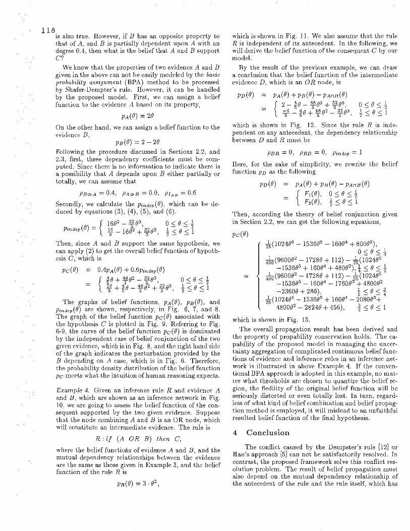
118

. 1

... ,

is also true. However, if B has an opposite property to that of A, and B is partially dependent upon A with an degree 0.4, then what is the belief that A and B support C?

We know that the properties of two evidence A and B given in the above can not be easily modeled by the basic probability assignment (BPA) method to be processed by Shafer-Dempter's rule. However, it can be handled by the proposed model. First, we can assign a belief function to the evidence A based on its property,

PA(/J) = 28

On the other hand, we can assign a belief function to the evidence B,

PB(/J) = 2 - 2/J Following the procedure discussed in Sections 2.2, and 2.3, first, three dependency coefficients must be com­puted. Since there is no information to indicate there is a possibility that A depends upon B either partially or totally, we can assume that

PB-:>A = 0.4, PA-:>B = 0.0, Phs = 0.6

Secondly, we calculate the Pindep(B), which can be de­duced by equations (3), (4), (5), and (6) .

{ 161]2 - 321]3 0 < /} < l

Pindep ( /J) = .!§. _ 15J2 +' 321]3 l < /} < 1 3 3 ' 2- -

Then, since A and B support the same hypothesis, we can apply (2) to get the overall belief function of hypoth­esis C, which is

Pc( IJ) 0 ::; /} ::; ! !::;B::;1

The graphs of belief functions, PA(/J), PB(/J), and Pindep(/J) are shown, respectively, in Fig. 6, 7, and 8. The graph of the belief function pc (/J) associated with the hypothesis C is plotted in Fig. 9. Referring to Fig. 6-9, the curve of the belief function pc (/J) is dominated by the independent case of belief conjunction of the two given evidence, which is in Fig. 8, and the right hand side of the graph indicates the perturbation provided by the B depending on A case, which is in Fig . 6. Therefore, the probability density distribution of the belieffunction Pc meets what the intuition of human reasoning expects.

Example 4. Given an inference rule R and evidence A and B, which are shown as an inference network in Fig. 10, we are going to assess the belief function of the con­sequent supported by the two given evidence. Suppose that the node combining A and B is an OR node, which will constitute an intermediate evidence. The rule is

R :i f (A ORB) then C,

where the belief functions of evidence A and B, and the mutual dependency relationships between the evidence are the same as those given in Example 3, and the belief function of the rule R is

which is shown in Fig. 11. We also assume that the rule R is independent of its antecedent . In the following, we will derive the belief function of the consequent C by our model.

By the result of the previous example, we can draw a conclusion that the belief function of the intermediate evidence D, which is an OR node, is

PD ( IJ) PA(/J) + PB(/J) - PAnB(/J)

{

2-1/}_48/}2+321]3 5 5 5 '

-6 _ 1/} + 481]2 _ 321]3 5 5 5 5 '

0 ::; /J ::; i i ::; /} ::; 1

which is shown in Fig. 12. Since the rule R is inde­pendent on any antecedent, the dependency relationship between D and R must be

PDR = 0, PRD = 0, Pindep = 1

Here, for the sake of simplicity, we rewrite the belief function PD as the following

PD(/J) PA(/J) + PB(/J) - PAnB(/J)

{ Fi ( /J) , 0 ::; /J ::; ! F2(/J) , i ::; /J::; 1

Then, according the theory of belief conjunction given in Section 2.2, we can get the following equations,

Pc(/J)

215(1024/}6

- 1536/J5 - 160/J4 + 800/J3),

0 ::; /} ::; i 4~0 (9600B2

- 1128/J + 112) - A (1024/J6

- 15361}5 + 1601}4 + 480/J3 ), i ::; I}::; ! 4~0 (9600/}2

- 1728/} + 112) - 215 (10241}6

-15361}5 - 160/J4 - 1760/J:r + 48001} 2

-2360/J + 280), ! ::; /J::; i A (1024/J6 - 15361}5 + 160/J4 - 2080B3+

48001}2 - 2824/J + 456), i ::; /J ::; 1

which is shown in Fig. 13. The overall propagation result has been derived and

the property of propability conservation holds. The ca­pability of the proposed model in managing the uncer­tainty aggregation of complicated continuous belief func­tions of evidence and inference rules in an inference net­work is illustrated in above Example 4. If the conven­tional BPA approach is adopted in this example, no mat­ter what thresholds are chosen to quantize the belief re­gion, the fiedility of the original belief function will be seriously distorted or even totally lost . In turn, regard­less of what kind of belief combination and belief propag­tion method is employed, it will mislead to an unfaithful resulted belief function of the final hypothesis .

4 Conclusion

The conflict caused by the Dempster's rule [12] or Hau's approach [5] can not be satisfactorily resolved. In contrast, the proposed framework solve this conflict res­olution problem. The result of belief propagation must also depend on the mutual dependency relationship of the antecedent of the rule and the rule itself, which has

long been ignored in the literature, in addition to the interpretations of the rule. The proposed model also embodies the inference in a lattice-structured inference network. Since an inference network can be treated as an AND/OR graph, the operation of any individual node (i.e., AND or OR) can reach the final result by applying the proposed model. If the node is AND, then it is con­sidered to be a Conj operation in the proposed model, while an OR node, then Union operation.

The new model offers several advantages over prior attempts. First, the conflict in the dependencies among the evidence in an inference network has been solved. Secondly, the discrete belief functions and the arbitrary continuous belief functions can be processed, which has not been researched to date. A continuous belief func­tion is extremely advantageous because it can represent the vagueness of a human concept more accurately than conventional means (i .e., BPA). Thirdly, the problem de­pendency propagation of an intermediate evidence has been resolved. Finally, the conflict of belief propaga­tion caused by the mutual dependency relationship of the antecedent of the rule and the rule itself has also been solved. This newly proposed strategy is intuitively closer to the intuitive reasoning process than is Demp­ster's consensus seeking strategy [11] [12] or Hau's com­promise seeking strategy [5], thus making this new model more successful and appealing than earlier attempts.

References

[1] Y. Cheng and R . L. Kashyap, "A study of asso­ciative evidential Reasoning," IEEE Trans. Pattern Anal. Machine Intell., vol.11, no.6, June 1989.

[2] P.R. Cohen, Heuristic reasoning about uncertainty: an artificial intelligence approach, Morgan Kauf­mann Publishers, Inc., Los Altos, California, 1985.

[3] R. 0. Duda, P. E. Hart, and N. Nilsson, "Subjective Baysian methods for rule-based inferen.ce systems," Proc. AF/PS, 1976.

[4] M. L. Ginsberg, "Nonmonotonic reasoning using Dempster's rule," Proc. National Con/. Artificial Intell. 1984, pp. 126-129.

[5] H. Y. Hau and R. L. Kashyap, "Belief combina­tion and propagation in a lattice-structured infer­ence network," IEEE Trans. Systems Man Cyber­net, vol. 20, no.l, Jan./Feb. 1990.

[6] R . A. Hummel and M. S. Landy, "A statiscal view­point on the theory of evidence," IEEE Trans. Pat­tern Anal. Machine Intell., vol. PAMI-10, no. 2, Mar. 1988.

[7] J. Ibara, "Extension of conditional probability and measures of belief and disbelif in hypothesis based on uncertain evidence," IEEE Trans. Pattern Anal. Machine Intell., vol. PAMI-9, no. 4, Jul. 1987

[8] M. Ishizuka, K. S. Fu, and J. T. P. Yao, "Inference procedure with uncertainty for problem reduction method," Information Sci. , vol. 28, pp. 179-206, 1983.

119 [9] K. B. Laskey, and P. E. Lehner, "Assumptions,

beliefs and probability," Artificial Intelligence, 41 (1989/90) 65-77.

[10] J. Pearl, "Fusion, propagation, and structuring in belief networks," Artificial Intelligence, 29 ( 1986) 24-1-288.

[11] G. Shafer and R. Logan, "Implementing Dempster 's rule for hierachical evidence," Artificial Intell., vol. 33, 1987.

[12] G. Shafer and J. Pearl, Readings in uncertain rea­soning, Morgan Kaufmann Publishers, Inc., San Mateo, California, 1990.

[13] P. P. Shenoy and G. Shafer, "Propagating belief functions with local computation," IEEE Expert, pp. 43-51, Fall 1986.

[14] H. Tahani and J. M. Keller, "Information fu­sion in computer vision using the fuzzy integral," IEEE Trans. Systems Man Cybernet, vol. 20, no.3, May/June 1990.

[15] L. E. Widman, K. A. Loparo and N. R. Nielsen, Ar7 tificial intelligence, simulation, and modeling, John Wiley & Sons Inc., 1989.

[16] J. Yen, "Generalizing the Dempster-Shafer theory to fuzzy sets," IEEE Trans. Systems Man Cybernet, vol. 20, no.3, May/June 1990.

[17] C.-C. Wang, and H.-S. Don, "A new approach to evidential reasoning by a potential model," Proc. ISMM Int. Con/. Computer Applications in Design, Simulation and Analysis, Las Vegas, Mar 1991.

[18] C.-C. Wang, and H.-S. Don, "A geometrical ap­proach to evidential reasoning," IEEE Int. Conf Systems, Man, and Cybernetics, Charlottesville, Virginia, Oct. 1991.

[19] L. A. Zadeh, "A simple view of the Dempster-Shafer theory of evidence and its implication for the rule of combination," Fuzzy Set Syst., vol. 11, 1983

(t, 1)

,.. , ,,_ .......... _ _,._a,o...._

·-

·I I

-:.1 . I

I .1

·1

120 C.. 1:

~ A0 •

c- ..

A8 ..... ,r... .......................

oftllrW....._...

~ Q

'II''

,..., ................ , ........... n.~ ......... ,........ ...... ., ... ..

.................... ............

:;: ,---.,-.,....--,--,--.---,--...... ----

'"··· F• I ..... t.MC._ .... ...._.. •f• ..... ~

.u:•

.......... I ,1 ... ,

, ... , ...... kac ...... -·~--h ...... l

•Jtl ::: .--.--,--,--,,--,--.--.--.--.--

,.,, ........... .,._..,..._ca1....,a .,.,, ___ ,,_ ..

~1 - -r---,- ···· 1·---·-r - --- ,· ---.- r·- --· r --·,-··· -

'\\ /" \ /.//

,, I I , , I \'-11··· .... , I 't1U1 1 U Ill 1) 0 LI :11 o -h f ot',H Ui.,• • , , ' 11 11 ,•..; . <1·11 1 I t ~ ,

fll.11 ....................... .._..Dlal ...... 4.

····, .!

0 ~

... 0

'tf.l ........... !M-.......... UN .. A ... a• la .... ).

::: ,-T"""-T"""-T"""-~~--,--,--,--,

/ /

, ,,'

,.,,,/

/

//~

//

.. 11:::-~~~--/,......, ......... , __..,-..J..-, _..___.._ ' 1)11t1 •! l U 11 11 11 ', ,i •l •h i , ,. ,,. 'IVd , , • U

Al, 11 ............................. ..

v\ .. . ~I ~/~~· ~~--, -l~ 'C) UU U I U U . • ll , 1 kJ <J 41.J 11 'JU U . l,41 U / tJ i i " '' IJ •Jl j I III J

A1,1, ............ ., .. c......-ca.....-4.

An Efficient Approach to Probabilistic Inference in Belief Nets *

Zhaoyu Li and Bruce D 'Ambrosio 303 Dearborn Hall

Department of Computer Science Oregon State University

Corvallis, OR 97331-3202 U.S. A.

zhaoyu©cs.orst.edu dambrosi©cs .orst.edu

Abstract

A number of exact algorithms have been devel­oped to perform probabilistic inference in be­lief nets in recent years. In general these al­gorithms have been developed from a graph­theoretic perspective. In this paper we con­sider probabilistic inference in a belief net from the combinatorial optimization point of view. Efficient probabilistic inference in a belief net can be seen as the problem of finding an opti­mal factoring given a set of probability distribu­tions to be combined. From this viewpoint , pre­viously developed algorithms are just different factoring strategies. We begin by defining the optimal factoring problem. We then present evidence for the utility of this perspective in the form of a very simple heuristic algorithm for factoring in multiply-connected networks. We show experimental evidence that this sim­ple greedy heuristic is more efficient than pre­viously developed exact probabilistic inference algorithms.

1 Introduction

A number of exact algorithms have been developed to perform probabilistic inference with belief nets in re­cent years. In general these algorithms have been de­veloped from a graph-theoretic perspective1 . Among the algorithms that have been developed are the propa­gation algorithms based on the original directed graph, such as the poly-tree propagation algorithm [Pearl, 1988; Pearl, 1986; Peot and Shachter, 1991), on a related di­rected graph, such as Symbolic Probabilistic Inference [D'Ambrosia, 1989; D'Ambrosia and Shachter, 1990) and Shachter's reduction algorithms [Shachter, 1986; Shachter, 1989; Shachter, 1988), or on a related undi­rected graph, such as Pearl's clustering and conditioning

*The authors gratefully acknowledge the support by NSF 91-00530 .

1 Shenoy's work [Shenoy, 1991) is very similar in spirit to ours. He studies inference under uncertainty from an al­gebraic perspective. However, he emphasizes mathematical foundations, whereas we emphasize algorithm development.

algorithms [Pearl, 1988) and Lauritzen and Spegielhal­ter's clustering algorithm [Lauritzen and Spiegelhalter, 1988).

The time complexity of probabilistic inference in a be­lief net is exponential in the number of nodes in the graph in the worst case. However, practical belief nets are usually only sparsely connected and we can take the advantage of conditional independence represented by sparseness of the graph to reduce the complexity of com­putation; that is, we may perform some non-numerical computation to reduce numeric computation. So, prob­abilistic inference in a belief net can generally be con­sidered as consisting of two components: numeric com­putation of the requested distributions and non-numeric computation or symbolic reasoning. For the above exact algorithms, the non-numeric computation of each algo­rithm is heuristic and is performed in polynomial time in the number of nodes of a belief net; but the time cost of numeric computation is exponential with respect to the maximum number of variables of two distributions to be combined in a query [Li, 1990). Therefore, the key point for speeding up a probabilistic inference algorithm is to reduce its numeric computation time. There are two ways to reduce the numeric computation time. One is to reduce the maximum dimensionality in the compu­tation by optimal arrangement of the computations to be performed. The second is to reduce the size of the computation by pre-computation or the re-structuring of the graph off-line. Pre-computation is not always ap­plicable. In this paper we will restrict our attention to finding more efficient factorings . Unfortunately, finding an optimal factoring is a hard problem.

Previous algorithms for inference in belief nets can be viewed as various heuristic strategies for factoring a product of a set of distributions. However, these strate­gies do not explicitly address the fundamental combina­torial optimization problem, and so may miss opportuni­ties for optimization. We begin by defining a combinato­rial optimization problem: Optimal Factoring. Then, we present a heuristic factoring algorithm. Finally, we show experimental results of the algorithm on randomly gen­erated belief nets and compare these results with those obtained by using the symbolic probabilistic inference (SPI) algorithm [D' Ambrosio, 1989], one of the most ef­ficient exact algorithms [Li, 1990).

The remainder of the paper is organized as follows.

121

I I

·· 1

122 Section 2 introduces a combinatorial optimization prob-lem - optimal factoring. Section 3 describes a heuristic factoring strategy we developed for multiply connected belief nets. Section 4 -shows experimental tests of the algorithm. Section 5 discusses the test results. Finally, section 6 discusses conclusions of the research.

2 Optimal factoring An optimal factoring problem (OFP) with n expressions can be considered as a combinatorial optimization prob­lem. Without loss of generality we assume that the do­main size of each variable is 2. The problem can be described as follows.

Definition 1 (FP) Given

1. a set of m variables V, 2. a set of n subsets of V: S = {S{1}, S{2} , ... , S{n}},

and 3. Q <; V is a set of target variables

define operations:

1. combination of two subsets S1 and SJ :

SwJ = S1 U SJ - {v : v (/. SK for K n J = ¢,,

K n J = ¢,, and v (/. Q},

I,J <; {1,2, .. . ,n}, InJ = ¢,; 2. the cost function of combining the two subsets:

µ(S{i}) = 0 for l $ i $ n, and

µ(SwJ ) = µ(S1) +µ(SJ)+ 2IS1uSJ I.

µ(S1 ) is not unique if II I > 2. In general, it depends on how we combine the subsets. We indicate these al­ternative combinations by subscripting µ. µa(S1) = µ shows the cost of combining result of S1 with respect to a specific tree structured combination of I, labeled a . We call this combination a factoring.

Definition 2 (OFP) An optimal factoring problem is to find a factoring a such that µa(S{i,2, ... ,n}) is min­imal.

In above definitions, Q is a set of target variables af­ter combining all subsets of S together; the set { v} in the formula SwJ is the variables which do not appear in the remaining subsets of S after combination of S1 with SJ . µa (SwJ ) is the total cost of combining all set S; ( i E J, J ) in a given factoring order, and is determined by the cardinalities of sets to be combined and affected by the size of { v} in previous combinations. If the do­main size of each variable is not limited to 2, the value 2l8 rUSJ I in above formula should be replaced with the multiplication of domain size of the variables in S1 U SJ . All possible factorings are equivalent to the results of permuting the n variables and then putting parenthe­ses in all possible ways in the permutation to form all S{i, 2 , ... ,n} 2 . It should be clear that determining the low­est cost way to combine distributions in a belief net is an OFP. The initial set of subsets is the set of sets each containing one variable ( or node) and its parents. The

2 The parentheses show the preference of combination.

reason that we do not restrict the appearance of variables in each subset S; is that some intermediate combination results or distributions still meet the definitions.

OFP generally is a hard problem. We suspect that OFP is an NP-hard problem, although do not yet have a proof-for this conjecture. Despite this, some restricted instances of OFP may have polynomial time algorithms. For example, given a domain of variables, if each pair of sets Si and Si is disjoint and the set Q is the union of all the sets Si; then the optimal ordering of a(S{i, , ... ,i,.}) could be obtained in linear time. Our specific interest is in the application of OFP to probabilistic inference.

One direct use of OFP is to find an optimal evaluation tree for computing queries in a belief net. Given a belief net with m nodes and some observations in it, a query involves identification of a subset n of the nodes relevant to the query, and computation of the conformal prod­uct [Shachter et al., 1990] of marginal and conditional probabilities of the n nodes. The n nodes with their re­lations can be mapped to the symbols in the definition of OFP: the n nodes with their immediate antecedent nodes are mapped to the n subsets of m variables; the queried nodes correspond to the variables in the sub­set Q; SwJ denotes the intermediate result of conformal product of distributions I and J; and µ gives the number of multiplications needed for the computation. Finding an optimal factoring minimizes the number of multipli­cations needed for this computation3 •

From the OFP point of view, we can see that previ­ously developed exact probabilistic inference algorithms are just different factoring strategies. However, these strategies didn't consider probabilistic inference as a fac­toring problem. We have proved [Li and D'Ambrosio, 1991] that there exists an optimal factoring algorithm which runs in polynomial time in the number of nodes for a poly-tree. However, finding an optimal factoring for an arbitrary belief net is a hard problem. In the next section we will present a heuristic algorithm for factor­ing an arbitrary belief net and show experimentally that this simple algorithm performs extremely well by testing it on randomly generated belief nets and comparing its results with those from SPI.

3 A heuristic factoring Algorithm

We now present an efficient heuristic algorithm, called set-factoring, we have developed for finding good fac­torings for probability computation. In a belief net with nodes {x1,x2, .. ,xn} connected by arcs, the general form of query is P(XJ IXK,XE), where XJ is a set of nodes being queried, XK is a set of conditioning nodes and XE is a set of observed nodes. P (XJ IXK, XE) can be com­puted from P(XJ,XKIXE) . For simplicity, we will only consider the case P(XJIXE) in the algorithm. This ig­nores several potential simplifications noted in [Shachter et al., 1990], but simplifies the presentation.

Given a query P(XJIXE) in a belief net, often only a sub-set of the nodes is involved in the probability com­putation. The involved nodes can be chosen from the

3 For proofs of the properties of probabilistic models which enable this a.lgebra.ic approach, see [Shachter et al., 1990].

original belief net by an algorithm which runs in time linear in the number of nodes and arcs in the belief net [Geiger et al., 1989]. Once we have obtained the nodes needed for the query, we have all the factors to be com­bined. In accordance with the definition 1, we have n sub-sets of n nodes and set Q. We use the following al­gorithm to combine these factors .

l. Construct a factor set A which contains all factors to be chosen for the next combination. Each fac­tor in set A consists of a set of nodes. Initialize a combination candidate set B empty.

2. Add any pairwise combination of factors of the fac­tor set A to B if the combination is not in set B, except the combination of two factors in which each factor is a marginal node and they have no com­mon child; and compute the u = (xUy) and sum(u) of each pair. Where x and y are factors in the set A, sum(u) is the number of nodes in u which can be summed over when the probability computation corresponding to the two factors is carried out.

3. Choose elements from set B such that C = { uiu : minimumB(lul - sum(u))}, here lul is the size of u excluding observed nodes. If ICI = 1, x and y are the factors for the next combination; other­wise, choose elements from C such that D = { ulu: maximumc(lxl+IYI), x, y Eu}. If IDI = 1, x and y are the terms for the next multiplication, otherwise, choose any one of D.

4. Generate a new factor by combining the candidate pair chosen from above steps and modify the factor set A by deleting two factors of the candidate pair from the factor set and putting the new factor in the set.

5. Delete any pair of set B which has non-empty inter­section with the candidate pair.

6. Repeat step 2 to 5 until only one element is left in the factor set A which is the final combination.

Following is an example to illustrate the algorithm by using the net shown in figure l. Suppose that we want to compute the query p( 4) for the belief net and assume that there are 2 possible values of each variable. The nodes relevant to the query are {1, 2, 3, 4}. We use the set-factoring algorithm to get their combination.

Loopl : factor set A is {1,2,3,4}; The set B is {(1,2) (1,3) (1,4) (2,3) (2,4) (3,4)} after step 2; the current combination is (1,2), i.e. p(2ll) * p(l) after step 3 (there was more than one candidate in this step, we chose one arbitrarily); the set A is {(1,2), 3, 4} after step 4; and the set B is {(3,4)} after step 5.

Loop2: factor set A is {(1,2),3,4}; The set B is {((1,2),3) ((1,2),4)) (3,4)} after step 2; the current com­bination is ((1,2),3) after step 3; the set A is {(1,2,3), 4} after step 4; and the set B is empty after step 5.

Loop3: factor set A is {(1,2,3),4}; The set B is {((1,2,3),4)} after step 2; the current combination is ((1,2,3),4) after step 3; the set A is {(1,2,3,4)} after step 4; and the set B is empty after step 5. The factoring

result is

p(4) = 1:(p(412,3H1:(p(3 ll)(p(211)p(1mn. 2,3 1

Figure 1: A simple belief net .

There are several things that should be noticed in the algorithm. First, queried nodes should not be deleted from any terms in the expression, and if a node is a queried node and it has no parents then the node will be combined after all other nodes are combined. Second, we assume that the number of the values of all nodes is same in the algorithm. If the numbers of values of the nodes in a belief net are different, we can consider the product of the number of values of all nodes related in each step instead of the number of nodes. Third, a caching strategy can be used in the algorithm. A caching table is generated before any query. Before combining any two factors, we check the caching table to see if there is a cached result for the combination. If there is a cached result, we can use the cached result at a cost of 0 instead of doing the real probability computation. If there is no such a cached result, then real computation will be carried out . This caching strategy will save some computation time.

The heuristic strategy in the algorithm can be ex­plained as follows: In step 2, (x Uy) shows the number of multiplications needed for combining the pair x and y4 • The elements in the set B are the candidates for the next combination. We don 't consider pairs consisting of two unrelated marginal nodes if they don't have common children since a combination of the two marginal nodes will usually increase dimensionality. In step 3, we choose the pairs which have the lowest result dimensionality as candidates since the best result of the current combina­tion may need less multiplications than those of the other combinations for subsequent combinations. The effect of summation is considered here; it always decreases the di­mensionality of the result. If more than one candidate is generated here, we choose the maximum (lxl + IYI) in step 4 as a criterion because this choice maximizes the number of variables being summed over. Usually, it is better to sum over variables as early as possible. Steps 4 and 5 are just preparations for the next loop .

The time complexity of the algorithm is dominated by the number of nodes related to the current query. Step

4 The number of multiplications should be 2lzuy l.

1 23

. I . - 1

I . _,

124 1 is linear in the number of nodes. In step 2, there are n * (n - 1)/2 pairs to be computed for the set B at the first loop, and (n- k) new pairs are added in the set at the end of the kth loop . There is a total of (n * (n -1)/ 2) + Z:k(n - k) = (n2 - 3n + 3) pairs are computed. For each pair, the union operation is O(m), here mis the maximum size of x; and sum(u) can be computed at the same time as computing ( x Uy). So the time complexity in step 2 is O(n3

) at most . The time cost of step 3 is linear in the number of pairs left in the set B and set C respectively, it is at most O(n2 ) including (n-1) loops needed for the two steps. Modifying the factor set in step 4 is linear in the number of factors, it has at most n eiements. Deleting some eiements from the set B in step 5 is linear in the number elements in the set. The time complexity is O(n2 ) in step 4 and O(n3 ) in step 5 including (n-1) loops for the algorithm. Therefore, the time complexity of the algorithm is O(n3 ) in the number of nodes.

4 Experimental tests

Time complexity of some currently used exact probabilis­tic inference algorithms, conditioning, clustering, reduc­tion and SPI, have been analyzed, and their efficiency has been experimentally tested [Li, 1990] with the im­plementation of IDEAL system [Srinivas and Breese, 1989] for conditioning, clustering and reduction algo­rithms and the implementation of SPI [D'Ambrosio, 1989]. Since SPI had better performance in that study than the others, we just experimentally compare set­factoring with SPI in this section.

Three sets of test cases were generated for time com­plexity experiments. We used J. Suermondt 's random net generator to generate all test cases. This generator starts with a fully connected belief net of size n, and re­moves arcs selected at random until the number of the remaining arcs is equal to a selected value. In each test case, we randomly5

, (ranging from 1 to the number of nodes in the belief net), determined the number of obser­vations to be inserted in that test case; then we randomly chose each observation from all unobserved variables in the belief net and finally we chose at random a set of variables as queries from remaining variables after each observation. The number of multiplications needed for each test case was recorded.

The first set of test cases is randomly generated with from 1.0 to 3.0 arcs per node and 8 to 13 nodes. The reason for choosing a set of small belief nets for testing is because we want to compare the results of set-factoring with those of an optimal algorithm, which is limited to run small belief nets because of time complexity6 • Ta­ble 1 shows the characteristics of the 10 test cases and the computational results of different algorithms measured in the number of multiplications: nodes is the number of nodes in each belief net; arcs/node is the average arcs per node; obs is the number of observations inserted in

5 Unless noted otherwise, all random selections are from uniform distributions over the indicated range.

6The optimal algorithm is a dynamic programming algo­rithm with exponential cost.

the belief net; and query is the total number of queries. The last three columns give the results of the generalized SPI [D'Ambrosio and Shachter, 1990], the set-factoring algorithm and the optimal algorithm respectively. From the table we see that the set-factoring has a better fac­toring result than the generalized SPI" but is not optimal in two test cases.

The second set of test cases is tree-structured belief nets. They are randomly generated with from 10 to 30 nodes. Table 2 shows the 10 belief nets and the test results. The columns 2 to 4 show the number of nodes, the number of observations and the number of queries for each test case. The columns 5 to 7 show the test results for each algorithm as in table l. From the table we see that the set-factoring has an optimal result for each tree structured belief net. The generalized SPI did not get optimal results for some test cases.

The third set of test cases is that used in testing SPI and Generalized SPI [D'Ambrosio, 1989; D'Ambrosio and Shachter, 1990; Shachter et al., 1990]. They are randomly generated from 1.0 to 5.0 arcs per node, and 10 to 30 nodes. In table 3, node shows the number of nodes and arc shows the number of arcs in each be­lief net; the columns obs and query give the the num­ber of observations and total queries in each test case respectively; and the rest of columns shows the num­ber of multiplications for each test case. A new version of SPI is used for comparison. SPI( cache) and set­fact (cache) show the results with intermediate result caching for both algorithms7•

From the above experimental results we see that the factoring strategy of set-factoring has better factoring re­sults than those of SPI in every case, particularly when a belief net is large. The number of multiplications in set-factoring is about half of those in SPI on average. Set-factoring is more consistent with respect to tasks and different kinds belief nets. As shown in table 3, set-factoring is better than SPI with caching for a large belief net, taking net 16 as an example. Since dimension in a factor will become large after some combinations, any bad combination order will cause many more multi­plications than a good combination does.

The time complexity of factoring for set-factoring and the time complexity of symbolic reasoning for SPI are only slightly different . In set-factoring, the time com­plexity is O(n3 ) in the number of nodes concerned in

· the current query at most; in SPI the time complexity is O(n3 ) at most in the number of nodes of the belief net . There should be no big difference. The time cost for symbolic reasoning in both algorithms is trivial com­pared to probability computation.

5 Discussion

While these results are preliminary, they seem a strong indication that the set-factoring algorithm is able to find better factoring for many problems, particularly in find­ing optimal factoring for all tree test cases. Also the set-factoring algorithm can be used as a suitable ana-

1 * denotes that corresponding algorithm is too slow to run the test case.

net nodes arcs/node obs query G.SPI set-factormg opt-alg 1 12 2 3 7 287 52 52 2 11 2.5 3 7 328 196 196 3 9 2.5 4 12 301 252 252 4 11 2 4 4 58 26 26 5 9 2.2 1 3 140 102 102 6 8 2.6 2 4 200 194 186 7 13 1 3 7 109 38 38 8 13 2.5 3 8 2760 1818 1716 9 13 2.4 3 8 144 94 94

10 10 1.7 3 7 237 174 174

Table 1: Ten small test cases and the test results by algorithms: the generalized SPI, the set-factoring and the optimal algorithm.

net nodes obs query G.SPI set-factormg opt-alg 1 23 6 68 728 646 646 2 19 19 89 1881 630 630 3 28 1 4 36 36 36 4 22 16 104 2959 1246 1246 5 17 7 34 809 404 404 6 12 9 27 335 148 148 7 24 17 128 1469 68 68 8 25 1 10 222 178 178 9 24 5 58 1478 1010 1010

10 22 5 46 1427 642 642

Table 2: Tree structured test cases and test results by algorithms: the generalized SPI, the set-factoring and the optimal algorithm.

net node arc obs query SPI set-factoring SPl(cache) set-fct (cache) 1 23 28 10 13 164 98 140 60 2 13 62 7 6 832 718 368 310 3 13 61 10 4 62 44 32 28 4 18 85 10 8 624 558 422 418 5 16 54 8 9 2,370 1,512 866 898 6 17 34 8 9 2,616 890 1,176 502 7 23 60 10 12 37,514 5,272 10,078 2,978 8 10 15 5 5 286 182 222 92 9 27 35 13 14 1,122 644 800 244

10 12 26 5 7 780 386 452 194 11 23 87 10 12 183,296 73,804 65,216 26,540 12 11 36 5 6 1,896 1,126 668 598 13 14 15 7 6 454 228 264 92 14 16 40 8 8 8,416 3,112 2,204 1,940 15 19 76 9 10 81,696 23,590 13,380 10,462 16 29 131 1 28 "' 6,569,756 16,146,192 3,196,900 17 29 90 14 14 1,489,040 143,334 254,292 73,146 18 16 35 9 6 2,480 898 816 450 19 15 53 7 8 15,986 4,168 3,068 1,896 20 26 101 13 13 717,552 124,734 113,248 63,834 21 28 34 14 13 2,052 847 1,384 330

Table 3: The experimental results of 21 test cases between SPI and set-factoring.

125

126

-I

lytical tool for evaluating other probabilistic inference algorithms. The most important conclusion from the experimental results is that OFP is a useful way of effi­ciently solving probabilistic inference problems in a belief net. From the OFP point of view, not only can we get a better algorithm than previously those developed, but also the algorithm is easy to understand and implement.

The main idea behind the set-factoring algorithm is, at each step, to find a pair with the best combination result . We tried the strategy of finding the pair with minimum multiplication as a candidate for combination; the re­sults are not as good as those obtained by set-factoring. The set-factoring algorithm only considers information iocaily for choosing each pair, so it can be implemented efficiently. It is this characteristic that prevents the al­gorithm from guaranteeing an optimal result for some multiply connected belief nets, because optimal results are related to all nodes concerned. It also tells us why the algorithm is good in tree structured belief nets: the factoring information for the tree is locally determined. Due to the locality of its heuristic strategy, set-factoring can work as a local factoring strategy in other proba­bilistic inference algorithms.

Since the last several combinations in factoring usu­ally have large dimensionality, combinations of the last few factors are critical in getting nearly optimal result for some belief nets. Considering this, we combined the set-factoring and the optimal algorithm together to get a new algorithm in which we used set-factoring to generate a partial result first and then used the optimal algorithm to complete the last several combinations. Since the op­timal algorithm can run efficiently for about 8 factors, the combined algorithm should run efficiently as well. The results of the combined algorithm are better than the set-factoring algorithm, particularly for large belief nets8 • This lead us to think of another factoring strategy of using the optimal algorithm. That is, if a belief net can be divided into several connected parts, we might use optimal algorithm within each part and then among all parts. We have not tested this idea yet.

The test result of the net 3 in table 3 for set-factoring (without caching) is optimal for each query, but both algorithms with caching give better results for the same queries. This indicates that a best probabilistic inference algorithm may not only depend on an optimal factoring strategy, but also depend on a good caching method for some tasks and some belief nets. There is a trade off between using a good factoring strategy and using an effective caching method in an inference algorithm, since a good factoring strategy flexible across many belief nets and tasks may be hard to combine with any caching method.

We have also studied the opportunities for parallelism in belief net inference. Set-factoring has shown good factoring results for parallel probability computation [D'Ambrosio et al., 1992].

8 Take the net 16 in table 3 as an example, the number of multiplications needed by the combined algorithm is about 75% of those by set-factoring.

6 Conclusions

In this paper we have presented a combinatorial opti­mization problem, optimal factoring. We have proposed that efficient probabilistic inference in a belief net can be considered as an optimal factoring problem. We be­lieve that it is a proper way to study the problem. From this point of view, finding an efficient exact probabilistic inference algorithm is the problem of finding an optimal factoring algorithm. Unfortunately, finding an optimal factoring in general is a hard problem. Currently de­veloped algorithms rely on structural properties of the graph to guide factoring . However, it is not clear this is the most direct way to find efficient factorings. We presented a heuristic factoring algorithm for multiply connected nets which makes no reference to graphical structure and yet outperforms current graph based algo­rithms.

References

[Srinivas and Breese, 1989] Sampath Srinivas and Jack Breese. IDEAL: Inference Diagram Evaluation and Analysis in Lisp, Documentation and Users Guide. Rockwell International Science Center, Palo Alto Laboratory, May 1989

[D'Ambrosio, 1989] Bruce D'Ambrosio. Symbolic Prob­abilistic Inference in Belief Networks. OSU technical report. December 1989.

[D'Ambrosio et al. , 1992] Bruce D'Ambrosio, Tony Fountain and Zhaoyu Li. Parallelizing Probabilistic Inference - Some Early Explorations. Submitted to the Eighth Conference on Uncertainty in Artificial Intelligence.

[D'Ambrosio and Shachter, 1990) Bruce D'Ambrosio and R. Shachter. Factoring Heuristics for General­ized SPI. OSU technical report. March 1990.

[Geiger et al., 1989] D. Geiger, T. Verma and J . Pearl. d-separation: From Theorems to Algorithms. Pro­ceedings of the fifth Workshop on Uncertainty in Ar­tificial Intelligence, pages 118-125. Windsor, Ontario, 1989.

[Lauritzen and Spiegelhalter, 1988] S. L. Lauritzen and D. J . Spiegelhalter. Local computations with Prob­abilities on Graphical Structures and Their Appli­cation to Expert Systems. Royal Statistical Society, pages 157-224. January 1988.

[Li, 1990] Zhaoyu Li. Complexity of Probabilistic Infer­ence in Belief Nets - an Experimental Study. MS the­sis, OSU. November 1990.

[Li and D'Ambrosio, 1991] Zhaoyu Li and Bruce D' Ambrosio. Probabilistic Inference in Belief Nets -A Combinatorial Optimization Problem. OSU, Oct, 1991.

[Pearl, 1988] J. Pearl. Probabilistic Reasoning in Intelli­gent Systems. Morgan Kaufmann, San Mateo, 1988.

[Pearl, 1986] J . Pearl. Fusion, Propagation, and Struc­turing in Belief Networks. Artificial Intelligence, 29(3): 241-288, 1986.

[Pearl, 1990] J. Pearl. Reasoning with Belief Functions: An Analysis of Compatibility. International Jour­nal of Approximate Reasoning, vol 4, pages, 263-289. September/November 1990.

[Peot and Shachter, 1991] Mark A. Peot and Ross D. Shachter, Fusion and Propagation with Multiple Ob­servations in Belief Networks. Artificial Intelligence, 48: 299-318, 1991.

[Shachter, 1986] R. D. Shachter. Evaluating Influence Diagrams. Operation Research, vol 34, pages 871-882, November 1986.

[Shachter, 1989] R. D. Shachter. Evidence Absorption and Propagation Through Evidence Reversal. Pro­ceedings of the Fifth Workshop on Uncertainty in Ar­tificial Intelligence, pages 303-310, 1989.

[Shachter, 1988] R. D. Shachter. Probabilistic Inference and Influence diagrams. Operations Research, Vol. 36, pages 589-604, July-August, 1988.

[Shachter et al., 1990] R. D. Shachter, Stig K. Ander­son and Kim L.Poh. Directed Reduction Algorithms and Decomposable graphs. Proceedings of the Sixth Conference on Uncertainty in Artificial Intelligence, pages 237-244, 1990.

[Shachter et al. , 1990] R. D. Shachter, B. D'Ambrosio, and B. D. Favero. Symbolic Probabilistic Inference in Belief Networks. Proceedings, Eighth National Con­ference on AI, pages 126-131, 1990.

[Shenoy, 1991] Prakash Shenoy. Independence In Valuation-based Systems, School of Business, University of Kansas, Nov. 1991.

127

!?8

.1

Definite Integral Information

Scott D. Goodwin Dept. of Computer Science

University of Regina.

Eric Neufeld Andre Trudel

Regina., Saskatchewan, Canada., S4S OA2

Dept. of Computational Science University of Saskatchewan Saskatoon, Saskatchewan,

Canada., S7N OWO

Jodrey School of Computer Science Acadia. University

Wolfville, Nova. Scotia., Canada., BOP lXO

( 306) 585-4 700 goodwin@cs.uregina..ca.

(306) 966-4887 eric@USask.ca.

(902) 542-2201 trudel@Aca.dia.U .ca.

Abstract Given vague temporal information about an interval, we wish to draw reasonable infer­ences about interior points and subintervals. Within the deductive framework of probability, such queries are sufficiently underconstrained as to result in degenerate answers. We show that when vague temporal information is rep­resented in the form of definite integral infor­mation, we can nonmonotonically infer answers to such queries that are both more interesting and useful. The inductive inference is achieved by identifying temporal intervals with reference classes and choosing the most specific. We also consider the effect of other knowledge- for in­stance, the knowledge that temporal informa­tion is true throughout some subinterval.

1 Introduction We study a previously undefined yet important class of temporal interval based information we call definite in­tegral information. An example of a problem involving such information is:

Over the year, it rains 40% of the time. Dur­ing winter (December 21- March 20), it rains 75% of the time. Over the summer (June 21 -September 20), it rains 20% of the time. What percentage of rainfall occurs during December? What is the chance of rain at midnight on De­cember 24th?

To obtain useful answers to these questions, it is neces­sary to go beyond what deductively follows from proba­bility theory.

The non-deductive reasoning we wish to do with defi­nite integral information requires nonmonotonic "jump­ing to conclusions" about subintervals and points based on interval information . In the absence of "other infor­mation," we assume that every point has an equal chance of having some property. We usually do have "other in­formation" and want to consider each point with respect to its most specific reference class, the narrowest class to which it belongs and for which we have "adequate" in­formation [Reichenbach, 1949; Kyburg, 1983]. Our view of what constitutes the narrowest reference class differs

from the commonly held view. We adopt recent ideas about inheritance of statistical information where infor­mation about a class of individuals has (the usual) down­ward influence on subclasses and has (a previously un­considered) upward influence on superclasses [Goodwin, 1991]. This lets us deal with conflicting sources of statis­tical knowledge by averaging the influences (i .e., a sort of "maximum entropy weighted average").

Such inferences require reasonable inductive assump­tions. Here we develop a probabilistic framework in which subinterval and point information is nonmono­tonically inferred directly from definite integral infor­mation . This direct inference hinges on an assump­tion of epistemological randomness, that is , if accord­ing to our current knowledge a particular point is in­terchangeable with any other point in some interval for which we have definite integral information, then the probabilistic properties of the point can be reasonably assumed to correspond to statistical properties of the interval. In a similar fashion, particular subintervals can reasonably be assumed to inherit statistical prop­erties from the interval. The problem of applying def­inite integral information to subintervals and points is related to the idea of direct inference in statistical rea­soning [Pollock, 1984]. Direct inference is the applica­tion of statistical information about a reference class to a member of the class. When there are multiple appli­cable reference classes, we must choose between them­this is the reference class problem [Reichenbach, 1949; Kyburg, 1983]-here we adopt the reference class selec­tion policy proposed in [Goodwin, 1991].

We also consider the effect of information such as con­tinuity. If we know the percentage of rainfall during an interval, the additional knowledge that the rain fell con­tinuously constrains the assumptions we can make about the distribution. In Section 5, we discuss how to reason in this case.

2 Definite integral information

The first order temporal logic we use is a variant of GCH [Trudel, 1990]. Point based information is represented with a function (J(t) which equals unity if (J is true at time point t, and equals zero otherwise. For example, "walking at time 3" is represented as walking(3) = 1. Our unorthodox representation of point-based informa-

R3: ?? r··-- -·- ...... , I I

Figure 1: Rainfall Summary

tion facilitates the representation of interval based infor­mation. Since the function /3(t) is a 0-1 valued function, we can integrate it over an interval to get the duration of truth of /3 over the interval. For example, if John is walking continuously between times O and 7, then :

Vt. 0 S t S 7 - walking(t) = l. We integrate to get the length of time (in this case 7 time units) that John is walking over the interval (0,7] :

17

walking(t)dt = 7. (1)

The value of the integral need not equal the length of the interval. For example, walked for 6 hours during some 10 hour period is represented as:

1to+lO

walking(t)dt = 6. to

(2)

Note that walking may not have occurred for 6 consecu­tive hours. It may have been interrupted many times.

Interval based information /3 is defined to be definite integral information if it can be represented in terms of a definite integral:

where O S a S (t2 - ti). For example, formulas (1- 2) describe definite integral information.

The rainfall example from Section 1 (summarized in Figure 1) is another example involving definite integral information. The GCH representation is given in Fig­ure 2. Here janl.s and janl.e refer to the start and end of January 1st respectively.

3 Examples

Using the rainfall example of Figure 1, we present dif­ferent examples of reasoning with definite integral infor­mation.

3.1 Interior point inferences

How likely is it to be raining at midnight on De­cember 24th? That is, what is the chance that raining(dec24.e) = 1: Notice that dec24 .e falls within the following reference classes ( refer to Figure 1) :

R1 = (janl.s, dec31.e], R 2 = (janl.s, mar20 .e] + (dec21.s, dec31.e], R3 = (decl.s, dec3I.e] .

129

1dec31.e

raining(t)dt = 0.4 x (dec31.e - janl.s) J anl.•

1dec31 .e

raining(t)dt = 0.75 x (dec31.e - dec21.s) dec2 l.•

1mar20.e

raining(t)dt = 0.75 x (mar20.e - janl.s) ;anl .•

r,ep20.e

}; raining(t)dt = 0.2 x (sep20.e - jun2I.s) jun21.•

janl.s = 0 I\ janl.e = l /\ .. . /\ dec31.e = 365

Figure 2: Rainfall Formulas

R3 is not useful because we cannot deduce any useful statistics about it from the axioms of Figure 2 ( and the axioms of probability) . We also choose to ignore R1 since R2 is a narrower (more specific, more relevant) reference class. We base our inferences about dec24.e on the ref­erence class R2 . According to our current knowledge, all the points within R2 are indistinguishable with respect to rain/ all so we assume every point in R 2 has the same chance of rain and conclude a 75% chance of rain at time dec24 .e.

3.2 Subinterval inferences

What percentage of rainfall occurs in December? The actual percentage of rainfall in December is:

rdec31 .e . , (t)dt Jdecl.• raining

(dec31.e - decl .s)

where the value of the numerator is unknown. To compute the amount of rainfall in December we divide the month (region R3 from Figure 1) into subregions R3a = (decl.s, dec20 .e] and R3b = (dec21.s, dec31.e] .

The narrowest reference class that contains R3a is

Rs = ( mar21.s , jun20 .e] + (sep21.s, dec20 .e] = R1 - R2 - R4 .

The statistic for Rs can be computed from the statistics for R1, R2 , and R4 , and from the relative sizes of these intervals . We compute the actual percentage of rain Ps over Rs to be:

p, - 0.4 X IR1I - 0.75 X IR2I - 0.2 X IR41 5

- IRsl _ 0.4 X 365-0.75 X (79+ 11] - 0.2 X 92

365 - (79 + 11] - 92

~ 33%.

By assuming every subset of Rs has the same expected percentage of rain, we conclude the expected percentage of rain over R3a is Ps.

The narrowest reference class (for which we have or can compute the actual percentage of rainfall) that con­tains R 3 b is R2. By assuming every subset of R 2 has

130 the same expected percentage of rain, we conclude the expected percentage of rain over Rab is 75%.

The expected percentage of rain over Ra equals a weighted average based on Raa and Rab:

P _ Ps x JRaa l + 0.75 x JRab l

a - JRa J

0.33 X 20 + 0.75 X 11 ~

31

~ 48%.

The answer to the original question is that it rams roughly half the time during December.

4 Direct inference rules

Let us now provide a formal characterization of the plau­sible inferences described in the previous section.

Definite integral information corresponds to a set of probabilistic constraints which determine a set of possi­ble interpretations. In general, we can only deduce weak constraints on subintervals and points from definite inte­gral information . For instance, from the rainfall example of Figure 2, the definite integral information that tells us that it rains 75% of the time in the winter, deductively implies that it rains between 50% and 100% of the time in the first half of winter . As for the individual points, we can only deduce that it may or may not be raining.

The plausible inferences we wish to make go beyond those deductively entailed by the definite integral infor­mation. They hinge on an assumption of epistemological randomness (or , roughly, a principle of indifference); that is, taking all we know into account, each possible inter­pretation is assumed to be interchangeable (i.e., equally expected). From this we can infer an expected value for the function /3 at a particular point. We can compute this value from the given definite integral information by first determining an interval of points, all of which have the same expected value for /3, and using definite integral information about the interval to determine the expected value at the particular point. This interval of points having the same expected value for /3 is a maxi­mally specific reference interval.

Definition 1 (MAX. SPECIFIC REF. INTERVAL)

The (possibly non-convex) interval R is a max­imally specific reference interval for f3 (t 0 ) if

l. to ER, and 2. /3 has the same expected value at every

point in R.

We do not need to know the expected value of /3 at ev­ery point in an interval to determine if it is maximally specific-we only need to know the expected values are the same. If the information we have concerning two points is identical ( with respect to /3), then the expected value of /3 at the points is the same. So all we need do is verify that we have the same information for every point in the interval.

Definition 2 (INTERCHANGEABLE POINTS)

Suppose the only definite integral information

our knowledge base contains concerning /3 is for the intervals: R1, R2, ... , Rn (we refer to these as explicit reference intervals for /3). We say two points t 1 and t 2 are interchangeable with respect to /3, by which we mean that /3 has the same expected value at t 1 and t2, if for every explicit reference interval R; for /3, we have t 1 E R; iff t2 ER;.

This says if the points fall within the same explicit refer­ence intervals, then the expected values are ( defined to be) the same.

Proposition 3 (FINDING MAX. SPEC. REF. !NT.)

If J is the intersection of the explicit reference intervals for /3 that contain the point t0 , and U is the union of the explicit reference intervals for /3 that do not contain the point t0 , then a maximally specific reference interval for /3( t0 )

is R = I - U.

Once we have identified a maximally specific reference interval for /3(to), we can relate the expected value of /3(to) to the definite integral information concerning the reference interval. To do this, we use the following prop­erty of mathematical expectation:

Proposition 4 (EXPECTATION OF SUMS)

For any interval I

E (1 /J(t)dt ) = 1 E((J(t))dt.

Interval I need not be convex. For example, if I = (x, y) U (u, v) and (x, y) and (u, v) are disjoint, then

f1 = J; +I:· Another useful property of mathematical expectation

is that the expected value of a constant is the constant.

Proposition 5 (PROPERTIES OF EXPECTATIONS)

For any interval I, expressions X, Y, and con­stant c

E(c) = c

E(cX) = cE(X) E(X + Y) = E(X) + E(Y).

We use Proposition 4 and the fact that the points of the reference interval have the same expected value for /3 to derive the following direct inference rule:

Proposition 6 ( DIRECT INFERENCE RULE 1) If R is a maximally specific reference interval for /3( to) then

E(/3(t0)) = E ( JR r~?dt) .

The expected value of /3 at to is equal to the average value of /3 over the interval R . Note that this follows trivially from the fact that /3 has the same value at every point in R since R is a maximally specific reference interval.

In the rainfall example (Figures 1 and 2), we com­pute the expected value for raining( dec24.e) as follows.

First, we identify a maximally specific reference interval for raining(dec24.e) using Proposition 3. Here we have R1 and R 2 as the explicit reference intervals for raining that contain dec24- e and R4 is the only explicit reference interval not containing dec24.e. So R = (R1nR2)-R4 = R2 is a maximally specific reference interval. The result E( raining( dec24.e)) = 75% now follows from Direct In­ference Rule 1, our definite integral information about R2 , and Proposition 5:

E( raining( dec24.e))

_ (JR1 raining(t)dt) - E IR2I

_ E (JR1

raining(t)dt)

IR2I

= E (0 . 75 x IR21)

IR2I 0.75 X IR2I

IR2I = 75%

Prop . 6

Prop . 5

Prop. 5

Another example is the computation of the expected value of raining(dec7.e):

E( 1·aining( dec7 .e))

= (JR, raining(t)dt) E IRsl

Prop. 6

E (JR, raining(t)dt)

IRsl Prop . 5

where R5 = R1 - ( R2 + R4 ) is a maximally specific refer­ence interval for raining(dec7.e) (by Proposition 3). We compute the numerator as follows:

E (l. raining(t)dt)

= E ( / raining(t)dt ) JR, - R1 - R•

= E (l, raining(t)dt

- [ raining(t)dt jR1

-l4

raining(t)dt)

= E(0.4 x 365 - 0.75 x 90 - 0.2 x 92)

= 60.1.

The value of the denominator is: IRs l = 365 - 90 - 92 = 183. So therefore: E(raining(dec7.e)) = 60.1/183 ::::::: 33%.

The following property is useful in relating subinter­vals to intervals:

Proposition 7 (DIRECT INFERENCE RuLE 2)

If S is a (possibly non-convex) subinterval of

Q, , 60% I I . I I 0 5 10 15

Figure 3: Overlapping reference intervals.

a maximally specific reference interval R for /3 then

(fs /3(t )dt) = (fR /3(t)dt)

E ISi E IRI . An example which uses Proposition 7 is the computa­tion of the expected value of raining over December. As in Section 3.2, we divide December into two subin­tervals Raa and Rab· By Proposition 3, we identify Rs = R1 - R2 - R4 as a maximally specific reference interval containing Raa and R2 as a maximally specific reference interval containing Rab· We then use Direct In­ference Rule 2 to relate the subintervals to the reference intervals . The computation of the expected values from the definite integral information about the reference in­tervals is then straightforward (see Appendix A) .

As a final example, suppose we know (see Figure 3) :

110

/3(t)dt = 6 I\ 115

/3(t)dt = 9.

Notice the explicit reference intervals Q1 = (0, 10] and Q 2 = [5, 15] overlap . For /3(7), we have Qa = Q1 n Q2 = [5, 10] is a maximally specific reference interval. We derive from the definite integral information that

fs 10

/3(t)dt E [4, 5]

and then by Direct Inference Rule 1, we have that

E (/3(7)) = E ( fs10 ~(t)dt ) E [l, 1].

5 Continuous definite integral information

If in addition to

110

walking(t)dt = 7,

we know that walking is uninterrupted (i .e., once the person starts walking, he walks for 7 consecutive time units), then this type of temporal information is called continuous definite integral information. Interval based information /3 is defined to be continuous definite integral information over some interval (t 1 , t 2 ) if:

1. J/1

2 f3(t)dt = a where O ~a~ (t 2 - ti), and

2. there exists a subinterval (ta, t4) of (t 1 , t2) such that

J/3• /3(t)dt = t4 - ta = a.

131

I

I

I

132 The direct inference rules from Section 4 are not ap­

plicable to continuous definite integral information . In­stead, we use the formulas presented below.

5.1 Interior point inferences

Given that walking is continuous definite inte­gral information over the interval (0,10) and that f0

10 walking(t)dt = 7, what is the chance that walking is true at times 0, 1, or 5? Intuition suggests that walk­ing is false at time O (there are an infinite number of subintervals of (0,10) of length 7 and only one of these subintervals contains the element 0) and true at time 5 (5 is an element of each subinterval of (0,10) of length 7) .

Formally, suppose we have continuous definite integral information about /3 over R = (Ra, Rb) where R is an interval of interchangeable points (see Definition 2) and JR /3(t)dt = L. To compute the expected value of /3 at a point t 0 in R, we use the proportion of subintervals of length L in R that contain ta:

E(f3(to)) = min(to, Rb ~bL2 ~ :a;,~Ra, to - L) . (3)

The term min( to, Rb - L) is the latest time and max( Ra, to - L) is the earliest time that a subinterval of length L that includes to could start. The denominator represents all the possible start times .

Returning to the walking example, the probability of walking at to = 0 is (0 - 0)/3 = 0. The probability at t 0 = 5 is (3 - 0) / 3 = 1 and the probability at t 0 = l is (1 - 0)/3 = 1/ 3.

5.2 Subinterval inferences

Once again , given that walking is continuous definite integral information over the interval (0,10) and that f

010 walking(t)dt = 7, what proportion of points in (0, 1)

is walking true? More generally, if (to, ti) is a subinterval of R =

(Ra, Rb), where R is defined as in Section 5.1 and letting I< = Rb - L - Ra, then :

E (1:• /3(t)dt) = 1:• E(/3(t))dt

Using equation 3, we substitute the integrand and obtain

JC 1 lti min(Rb - L, t) - max(Ra, t - L)dt to

= K - 1 (1:· min(Rb - L, t)dt

-1:· max(Ra,t - L)dt)

(1min(t1,R.+L)

- Radt min(to,R.+L)

rmax(R.+L,ti) )] +j (t - L)dt . max(R0 +L,to)

Returning to the walking example, we expect walking to be true at all points in (5, 6), at 1/6 of the points in (0, 1) and at 0.958333 of the points in (2.5 , 3.5) . As ex­pected, walking is true at greater proportions of intervals near the middle.

5.3 Continuous subinterval inferences

We now consider a variation of the problem dealt with in Section 5.2. Given that walking is continuous def­inite integral information over the interval (0,10) and that f0

10 walking( t )dt = 7, what is the probability that

walking is true throughout the interval (0.5, 1.5)? Note this is different from asking what proportion of points in (0 .5, 1.5) is walking true.

If R and L are defined as in Section 5 .1, then the probability /3 is true throughout (to, ti) ~ R is:

p (1:· /3(t)dt = ti - to)

= max 0, . ( L - (ti - to) )

IR I - (ti - to) This is a deductive consequence and requires no induc­tive assumption about probabilities at points.

Returning to the walking example, the probability that walking is true throughout (0, 1) is zero, throughout (5, 6) is 1.0, and throughout (0 .5, 1.5) is 0.05 .

6 Comparison with other work

The only previous attempt at representing a subset of definite integral information is Allen's processes [Allen , 1984]. Examples of processes are 'I am walking' and 'ran a while' over some interval. Questions have been raised about the correctness of Allen's representation (see [Trudel, 1992] for a discussion). Also, Allen does not consider the types of reasoning we are interested in.

Eberbach et. al. [Eberbach and Trudel, 1992] con­sider a problem which can be viewed as the opposite of that dealt with here. Instead of deriving probabilities at points based on interval based information, they be­gin with the probabilities at the points and then derive probabilities for the interval based information.

7 Conclusion

We have shown how to represent and reason with definite int,egral information-approximate knowledge about the duration of temporal information. Although very little can be said that is categorically true about any subinter­val or any specific point, many interesting results can be derived from the axioms of probability given the notion of inference from a maximally specific reference class. For example, given a set of temporal statistics, we have shown how to compute the probability that temporal in­formation is true at an interior point, the probability the information persists throughout a subinterval and the expected proportion of points at which temporal in­formation is true in a subinterval.

Acknowledgements

The first author acknowledges the support of the Insti­tute for Robotics and Intelligent Systems (IRIS). Re­search of the second author was supported by IRIS and NSERC grant OGP0099045. Research of the third au­thor was supported by NSERC grant OGP0046773. We thank Howard Hamilton for his comments.

Appendix A

The computation of the expected value of raining over December from the given definite integral information (see Figure 2) involves dividing December into two subin­tervals R3a and R3b· We then use Direct Inference Rule 2 in conjunction with the maximally specific reference intervals R5 = R1 - R2 - R4 and R2 as follows:

By Proposition 5,

( fR

3 raining(t)dt) _ E ( f R 3 raining(t)dt)

E IR3I - IR3I , Considering just the numerator,

E (l3

raining(t)dt) =

E (l3

• raining(t)dt) + E (l3

b raining(t)dt).

By rewriting Proposition 7 as

E (1 f3(t)dt) = E (fl;~t)dt) · ISi,

we can then write

E (1 raining(t)dt) R3a

and

E (l3

b raining(t)dt)

E (IR2

raining (t)dt)

IR2I · IR3bl , From previous computations, we substitute to obtain

E (1 raining(t)dt) :::::: 0.33. 20 R3a

and

E (l3

b raining(t)dt) = 0.75 · 11.

Then

E (l3

raining(t)dt) :::::: 0.33 · 20 + 0.75. 11

and

( f R raining(t)dt)

E 3 IR3I :::::: 48% .

References 133

[Allen, 1984) J .F. Allen. Towards a general theory of action and time. Artificial Intelligence, 23(2) : 123-154, 1984.

[Eberbach and Trudel, 1992) E. Eberbach and A. Trudel. Representing spatial and temporal uncertainty. In Fourth International Con­ference on Information Processing and Management of Uncertainty in Knowledge-Based Systems, Palma de Mallorca, Spain, 1992. [to appear) .

[Goodwin, 1991) S.D. Goodwin. Statistically Motivated Defaults. PhD thesis, Department of Computing Sci­ence, University of Alberta, Edmonton, Alberta, 1991. (also University of Regina Computer Science TR-91-03) .

[Kyburg, 1983] H.E. Kyburg, Jr . The reference class. Philosophy of Science, 50(3):374-397, September 1983.

[Pollock, 1984) J. Pollock. Foundations for direct infer­ence. Theory and Decision, 17:221-256, 1984.

[Reichenbach, 1949) H. Reichenbach. Theory of Prob­ability. University of California Press, Los Angeles, California, 1949.

[Trudel , 1990) A. Trudel. Temporal integration. In Pro­ceedings of the Eighth Biennial Conference on the Canadian Society for Computational Studies of Intel­ligence, pages 40-45, Ottawa, Canada, May 1990.

[Trudel, 1992) A. Trudel. A formal specification of Allen's processes. In European Conference on Artifi­cial Intelligence, Vienna, Austria, August 1992. [sub­mitted) .

134

I

A Characterization of Extensions of Gerneral Default Theory

Zhang Mingyi Guizhou Academy of Sciences

40 East Yanan Road, Guiyang City Guizhou Province, 550001, P.R. China

Abstract

A formalism for default reasoning introduced by Reiter [Reiter 1978a, 1978b, 1980, 1981, 1982], which provides a formal framework for an important part of human reasoning, ap­pears to be the most stable one of the ap­proaches to non-monotonic inference [Ginsbery, 1987]. However, Reiter and his followers have been placing a heavy emphasis on a class of so-called normal defaults since then, the rea­son why they do so seems to be that a general class of defaults is mathematically intractable [Reiter and Cirscuolo, 1981]. So up to now, the main point about general default theories remain unclear. In this paper a characteri­zation of extensions of general default theo­ries is given. Basded on this, several results on the existence of extensions are shown .All these essentially develop Reiter's theory and provide for introducing another class of de­faults, so-called Auto-compatible Default The­ory, which is more general than Normal Default Theory and enjoys very nice feature of the lat­ter [Mingyi, 1991a, 1991b].

Key Words : Default Theory, Extension of Default Theories, Compatible Subset of De­faults , Auto-compatible Default.

1. Introduction

Default reasoning is foundmental in Artificial Intelli­gence( AI) because it appears to be the only tractable method to deal with the problem of incomplete informa­tion and it is specifically concerned with common sense reasoning, which has recently been recognized in the AI literature to be foundamental importance for knowledge representation[Besnard, 1989].

A formalism for default resoning introduced by Re­iter[Reiter, 1978a], Default Logic, which puts forward the idea of using it as a knowledge represetation scheme

for an important part of human reasoning in AI, ap­pears to be the most stable: ahnost without exception, the articles that have appeared after Reiter's original one focus on applying Reiter's idea as opposed to modi­fying them. The single exception is Lukaszewicz's mod­ification[Lukaszewicz, 1984a, 1984b, 1985]. A number of people feel unconfortable with the face that not all theories of default logic have extension and that there is no proof theory worthy of this name of the whole logic. Lukaszewicz (1984b) has proposed an alternative view of the nation of extensions, one by which extensions ex­ist for any default theory. However, knowledge repre­sentation problems involving default reasoning need not be given solutions more conforming to everybody's intu­itions by Lukaszewicz's modified formalization of deriv­ability using default than by Reiter's original one. No Logic can be expected to be perfect for all cases for which it has been devised. to handle. There are always examples that can be given conterintutive or paradoxical inter­pretations. So default Logic cannot be attacked on the grounds that no particular approach to it deserves to be preferred over all others. In fact, Reiter's formalism al­lows for extending variations as well as for convervative variations ( e.g.Rychlik, 1985; Saint-Dizier, 1986, 1988; Etherigton, 1987; Froidevaux and Kagser, 1988; Mercer, 1987).

However, Reiter and his followers have been placed a heavy emphasis on the class of so-called normal de­faults and less concerned about the general class of de­faults since general default theories are mathematically intractable [Reiter and Cirscuolo, 1981]. Though it is so, Reiter et al. noticed that normal defaults can interact with each other in ways that lead to counterintutive re­sults and had to introduce a general class of so-called semi-normal defaults . Unfortunately, the semi-normal class lacks many nice features which are enjoyed by the normal class. Up to now, we little know intersting inves­tigation in this topic and main point about general de­fault theories remains unclear. In paticular, the problem on the existence of extensions of general default theories, which is complex and difficult to deal with, has been not explored.

Following a differet approach from one of [Reiter, 1980], this paper will explore the above mentioned prob­lem on the existence of extensions. Though Reiter gave a characterization of extensions (Theorem 2.1 [Reiter, 19801), it is faced with trouble testing an enormous col­lection of sets of closed wffs to determine if a default the­ory has an extension and such a testing is computation­ally intractable and inconvenient to investigation. So, we give a characterization of extensions , which depends only on the given information and default rules. Accord­ing to this, the sufficient c0nditions of [Mingyi, 1991a] becomes a direct result of the condition given by intro­ducing the notions of compatible subsets of defaults and auto-compatible defaults in the paper. All this provides for introducing another class of defaults, so-called Auto­compatible Defaults Theory [Mingyi, 1991b], which is more general than Normal Default Theory and enjoys very nice feature of the latter. It ' is worth noticing that the sufficient condition on the existence and unique­ness of extension for general default theories given in [Besnard, 1989](As far as we know, it is one of a few results on the existence of extesions expect Reiter's re­sult ) is just a corollary of our result, and Theorem 3 of [Wu, 1991] is only a particular example of the result of [Besnard, 1989]. Hence, our work is an essential devel­opment of Reiter's theory.

Following [Reiter, 1980], we use the following con­cepts and notations.

By a default 5 we mean any configuration of the form

a(x) : M[3i(x), ... Mf3n(x)!,(x)

where a (x), f3i(x), .. ,f3n(x), ,(x) are wffs whose free vari­ables are occur in x = x1 , ... , Xm· a (x) is called the prerequisite of the default, f3i( x), ... , f3n ( x) is called the consistency condition of the default 5, ,(x) is called the consequent of the default 5.

For simplicity, the form of a default 5 is usually abbreviated as a : M /31, ... , M f3nh provided it does not sacrifice clarity.

A default is closed iff none of a, /3 1 , .. . , /3n, , con­tains a free variable.

A default theory I:::. is a pair (D, W) where Dis a set of defaults and W is a set of closed wffs. If every element of D is closed, then ( D, W) is 01.lled a closed default theory. As in [Reiter, 1980], the technical results on closed default theories can be generalized to the case of open defaults by Skolemizing W as well as all of defaults of D. So there is clearly no ioss of generality by requiring wffs of Wand CON (D) to be closed. According to this, this paper only disscusses the closed default theories.

Given a closed default theory 6 = (D, W) and any D' ~ D, define

PRE(D') = {al(a : M/31, ... , M/3nh) E D'}

CON(D') = bl(a: M/31, ... , M/3n/,) ED'}

135 CCS (D') = {/3;l(a : M/31, ... , M/3n/,) E D'andl ~ i ~ n}

2. Existence of Extensions

In [Reiter, 1980] a characterization of extension by means of a sequence of sets of closed wffs(Theorem 2.l)is given by which we can determine if a set E of closed wffs is an extension of a closed default theory. Based on this, a few properties of default theories and a complete the­ory on the class of normal defaults are obtained.However, it is very difficult to decide whether a set of closed wff is an extension of a closed default theory by the condition since it needs to test an enormous collection of sets. So this obstructs further study on the general class of de­fault. In this section, it starts immidiately from a default theory's self to explore the problem on the existence of extensions. Unquestionably our result depending only given information W and the sets D of defaults is more simple and natural.

Definition 2.1: Let E be a set of closed wffs and 6 = (D, W) a closed default theory. Let us define

Eo(A) = W E;+i(l:::.) = Th(E;(t:::.))u{,l(a: M/31, ... , Mf3n/,) E

D where a E E;(!:::.)and-,/31, ... , -,f3n ¢ E}

Let

e(E, A)= LJ E;(A) O:Si<oo

For i > 0, define GD(E;(A)) = {(a : M/31, ... Mf3n/,) E Dia E E;-i(A)and-,/31, ... , -,f3n ¢ E}

and GD (Eo(A) ) = 0. Let GD(e(E, A), A) = Uo<i<oo GD(E;(A)). Usually, the symbol A in the notation E;(A) (i ~ O)

will be omitted if it does not make confusion. Definition 2.2: For any closed default theory

6 = (D, W), define Do(A) = {(a: M/31, ... , Mf3n/,) E DIW f- a}

and for i > 0, D;+i(A) = {(a M/31, ... , Mf3nh)IW u CON(D;(A)) f- a}

>.(D, A) = LJ D;(A) O'.Si <co

As the above, the symbol A in D;(A)(i ~ 0) and )..(D, A) will be omitted.

Notation: -,/31, ... , -,f3n ¢ E and S If -,{31, ... , -,f3n is an abbreviation for

-,/31 ¢ E , ... , -,f3n ¢ E and S If -,{31, ... , S If -,f3n , respectively.

It is easy to show that the following theorem is equivalent to Theorem 2.1 of [Reiter, 1980]. ·

Theorem 2.1.Let Ebe a set of closed wffs and A= (D, W) a closed default theory, then E is an extension of A iff E = e(E, A).

1 .J6

Corollary. Given a closed default theory A = ( D, W) and a set of closed wff s, then

e(E, A)= Th(W u CON(GD(e(E, A}, A}}).

Especially, if E is an extension of A then

E = Th(W u CON(GD(E, !:::..)).

Throughout the paper , GD(e(E, A), A}}) is re­placed by GD(E, A} when Eis an extension of A.

Definition 2.3. Let!:::..= (D, W) be a dosed default theory. D' ~ D is an incompatible subset of defaults with respect to!:::.. iff their is S = (a : M/31, ... , M f3nh) E D' such that WUCON(D'} I- -.f3i for some i, 1 :5 i :5 n. If D' is not incompatible then call it a compatible subset of defaults with respect to !:::... A compatible subset D* of defaults is maximally compatible subset of defaults iff' D* ~ D' implies D' = D*, where D' ~ D is any compatible subset of defaults.

Corollary 2.3.[Reiter, 1980] Any closed default theory has a maximally co:.apatible subset of defaults.

Proof: It is sufficient to notice that SD = { D' ~ D ID' is compatible} is not empty since efi E SD. The corollary is proved by Zorn's Lemma.

Defl..nition 2.4. Let 6. = (D, W) be a closed de­fault theory. A default

S = (a: M/31, ... , M/3nh) ED

is auto-incompatible with respect to A iff there exists a compatible subset D' of defaults such that

WuCON(D'} 'rj-.f31, ... ,-.f3n

and Wu CON(D' U {S}) I- ...,13

for some f3 E CCS(D' U {S}) . Here D' is said to be an associated auto-incomp;.tible subset of defaults with respect to S. And if S is not auto-incompatible then it is auto-compatible.

Corollary 2.4. Any closed default theory 6. = (D, W) with compatible subset D of defaults does not contain any auto-incompatible defaults .

Proof. It is clear from Definition 2.3 and 2.4. Lemma 2.5. Let E be an extension of a default

theory 6. = (D, W} then >.(GD(E, A}}= GD(E, A}. Proof. From Definitions 2.1 and 2.2 we have

>.(GD(E, A})= LJ (GD(E, A}}i O~i<oo

GD(E, !:::..} = LJ GD(Ei, A} O~i<oo

First, we prove by induction 0n i that (GD(E, A)), ~ GD(E2H2, !:::..).

Base: HS= (a: M/31, ... , M/3nh) E (GD(E, A))o then W I- a and -.{31, ... , -.f3n ~ E which implies

that a E E 1. So S E GD(E2, !:::..), that is, we proved (GD(E, !:::..))o ~ GD(E2, !:::..).

Step: Assume that (GD(E, !:::..))i ~ GD(E2i+2, !:::..). For any S = (a : M/31, ... , Mf3nh) E (GD(E, A))i+i then WLJCON(GD(E,!:::..)i) I- a and -.f31, ... ,-.f3n ~ E. By the induction assumption, WU CON(GD(E2i+2, A)) l­a . Therefore a E E2i+3.Hence SE GD(E2i+4, !:::..).

The result implies that >.(GD(E, !:::..)) ~ GD(E, !:::..). Similarly, we can prove by induction that

GD(Ei, !:::..) ~ GD(E, !:::..)i-1 for all i > 0. Base: It is clear that GD(E1, !:::..) ~ GD(E, !:::..)o, Step: Assume that GD(E,, A) ~ GD(E, A),-1

For any S = (a : M/31, ... , Mf3nh) E GD(EH1, !:::..), we have a EE, and -./31, ... -.f3n ~ E .So, a E Th(E,-d U CON(GD(Ei, !:::..)). Theorefore WuCON(GD(E,, !:::..)) l­a. By the induction assumption,

Wu CON((GD(E, 6.)),_i) I- a

which yields SE (GD(E, 6.)), The result implies GD(E, 6.) ~).. (GD(E, 6.)). And

all this complete the proof of the lemma. Theorem 2.6. Any closed default has an extension

iff there exists a compatible subset D· of defaults such that

Pl. >.(D*) = D* ~ D . P2. For any S = (a : M/31, ... ,M/Jnh) E D-D*,

either Wu CON(D*) 'r/ a or Wu CON(D*) I- -.(3, for some i, 1 :5 i :5 n.

Proof. The case where W is inconsistent is not con­sidered, as it makes the theorem trivial. In fact, 6. has a.n inconsistent extension iff W is inconsistent by corol­lary 2.2 of [Reiter, 1980]. At the same time, D* in the theorem is just empty.

(Only if part) ff 6. has a consistent extension E. First we show that GD(E, 6.) is compatible. Assume the contrary holds: there is S' = ( a' : M /3L ... , M f3'mh') E GD(E, 6.) such that W u CON(GD(E, 6.)) I- -.f3! for some i, 1 :5 i :5 m. Since E = Th(W U CON(GD(E, 6.))) it follows that -.f3f E E and this is a contradiction. So GD(E, 6.) satisfies Pl by Lemma 2.5.

Next , if there is S = (a : M/31, ... , Mf3mh) ED -GD(E, 6.) such that

Wu CON(GD(E, 6.)) I- a

and W u CON(GD(E, 6.)) 'r/ -./31, ... , -.f3n then o: E E,-.(31, ... , -.f3n ¢ E. Hence SE GD(E,6.). a con­tradition.That is, GD(E, 6.) satisfies P2.

(If part) Assume that D* is the compatible sub­set of defaults satisfing Pl an P2. Let E = Th(W U

CON(D*)). First we show by induction on i that e(E,!:::..) ~ E.

Base: Obviously, Eo s;;; E. Step: Assume that Ei s;;; E. Then Th(Ei) s;;;

E and Q E E, 1/31, ... , 1 /3n fl_ E for any 6 = (a : M/31, ... ,M/Jnh) E GD(E,+1,A) since Ei+i = Th(E,) u CON(GD(E,+1, A)). So 5 E D* (otherwise it would contradict P2). This implies E,+1 s;;; E.

Next we show E s;;; Ei(E, A). To prove this it is sufficient to show

D* s;;; GD(8(E, A), A) since E = Th(W u CON(D*)), W s;;; e(E, A) and

e(E, A) = Th(W u CON(GD(e(E, A), A))). In this similitude of the proof of Lemma 2.5, we show by induction on i that D*. s;;; GD(E2,+2, A).

Base: For any S = (a: M/31, ... ,M/3nh) E D*o, then WU CON(D*) If -,/31, ... ,-,f3n in view of the com­patibility of D* and a E E1 since WI- a. So 5 E E2,

Step: Assume (D* ), s;;; GD(Ezi+z, A) . Then for any 5 = (a : M/31, ... , Mf3nh) E (D*).+1, we have WU CON((D*).) I- a. By the induction assumption,

Wu CON(GD(E.+1, A)) I- a. So a E E2i+3· Hence WU CON(D*) If -i/31, ... , -i/3n by the compati­bility of D*. This gives 5 E GD(E2,+4, A) which yields (D*),+1 s;;; GD(Ez,H, A).

The result implies that D* s;;; GD(8(E, A), A) since D* = >.(D*) = Uo<,<oo(D*),. Therefore Es;;; e(E, A) . So, E = 8(E, A) and-Eis an extension of A by Theorem 2.1.

Theorem 2.1. Any closed default theory has exactly an extension iff there is a compatible sub­set of defaults satisfing Pl and P2 in Theorem 2.6 and for any such subsets of defaults D*, D**, W 1-1\CO N (D* ) <=> I\CON(D**) always holds, where the notation I\S means the conjunction of elements of any set S of wff, i.e. Aaes a .

Proof. It is sufficient to note that E 1 = E2 iff W 1-1\CO N (D* ) <=> I\CON(D**) . Where E 1 = Th(W u CON(D*)), E2 = Th(WuCON(D**)) . The remains of the proof is easy by Theorem 2.6.

Lemma 2.8. Given a closed default theory A = (D, W) and D', D" s;;; D. If D' s;;; D" then >.(D') s;;; >.(D"). As a result >.(>.(D')) = >.(D') for any D' s;;; D.

proof. The first part of the lemma is easily obtained by induction. For the seco1iJ part, it is easy to show that >.(>.(D')) s;;; >.(D') by Defii·. ition 2.2. Now we prove by induction on i that (D'), s;;; (>.(D'))..

Base: It is clear that (D')o s;;; (>.(D'))o, Step: Assume (D') i s;;; (>.(D')).. Then 5 E

>.(D') and W U CON((D').) I- a for any 5 = (a : M/31, ... , M/3nh) E (D') i+l· By the induction assump­tion,

Wu CON((>.(D'))i) I- a

which implies that 5 E (>.(D')) i+l· So, (D')i+i s;;; (>.(D')) .+1·

All of the above shows that >.(>.(D')) = >.(D') . The following consequence comes immidiately from

Lemma 2.8.

137 Corollary. Let D' be a maximally compatible

subset of defaults with respect to A = (D, W). Then >.(>.(D')) = >.(D') and >.(D') is also compatible.

Lemma 2.10. If a closed default theory A = (D, W) has an extension E, then there is a maximally compatible subset D* of defaults with respect to A such that GD(E, A)= >.(D*) .

Proof. The case where E is inconsistent is not con­sidered, as it makes the lemma trivial. By the proof of Theorem 2.6 we know that GD(E, A) is compat­ible and GD(E, A) = >.(GD(E, A)). So there is a maximally compatible subset D* of defaults such that GD(E, A) s;;; D* . By Lemma 2.8, GD(E, A) s;;; >.(D*). Let E* = Th(W u CON(D* )) . Clearly, E s;;; E* .Now we show by induction on i that (D* )i s;;; (GD(E,A)) ,, which implies that >.(D*) s;;; >.(GD(E, A ))) = GD(E, A) and that >.(D*) = GD(E, A).

Base: Clearly, (D* )o s;;; (GD(E, A))o.

Step: Assume (D*), s;;; (GD(E, A)),, then WU CON((D*).) I- a for any S = (a : M/31, ... , M/3nh) E (D*),+1· By the induction assumption, W U

CON((GD(E, A)),) I- a . Since -,/31, ... ,-,f3n ¢Eby the compatibility of D *. It follows that SE (GD(E,A))i+l · Therefore (D*).+1 s;;; (GD(E, A)).+1·

Theorem 2.11. Any closed default theory A = (D, W) has an extension iff there is a maximally com­patible subset D* of defaults with respect to A such that for any 5 = (a: M/31, ... , Mf3nh) ED - D*, either Wu CON(>.(D*)) If a or Wu CON(>.(D*)) I- -i/3, for some i, 1 ::::; i ::::; n.

The proof simply consists of an application of The­orem 2.6 and Lemma 2.10.

Remark. Theorem 2.11 provides for more simple and helpful schema to construct extensions of a closed default theory than Theorem 2.1 of [Reiter, 1980] does because it does not depend on any set E of closed wffs like one in Theorem 2.1 of [Reiter, 1980]. Assume that we can decide whether W U CON(D') I- a, -,13 hold for a given closed default theory A = (D, W) and any a, /3 E P RE(D) U CCS(D). To determine if A has an extension we need only to test every maximally com­patible subset of defaults with respect to A. In other words, for a given maximally compatible subset D * if there exists 5 = (a : M/31, ... , M/3nh) E D - D* such that Wu CON(>.(D* )) I- a and Wu CON(>.(D* )) If -i/31, ... , -if3n, then reject the D * and continue to test an­other maximally compatible subset of default. This test­ing will proceed till one of the following cases occurs:

C;:u;e 1. If all maximally compatible subsets of de­faults are rejected, then A has not any extension.

Case 2. If some maximally compatible subset D * of defaults is not rejected, then E = Th(WUCON(>.(D* ))) is one extension of A.

Clearly, This schema is more direct and helpful to finding extensions than one in [Reiter, 1980].

138

. ·1

3. Several Important Consequences

By using the nercessary and sufficient condition for the existence of extensions we obtain the following suffi­cient conditions which seems more important than those we know up to now.

Theorem 3.1. If a closed default theory A = (D, W) does not contain any auto-incompatible default then it has an extension.

Proof: In the case where Wis inconsistent, it is clear that D does not contain any auto-incompatible default and A has an inconsistent extension. So the theorem is true.

Now assume that W is consistent.First, if 0 is a max­imally compatible subset of defaults with respect to D... then 0 satisfies Pl and P2 m Theorem 2.6 since A does not contain any auto-incompatible default. Therefore D... has an extension E = Th(W) by Theorem 2.6. Next, suppose that A has a non-empty maximally compatible subset D* of defaults. For every D*, there are two cases to be considered.

Case 1. >.(D*) = D*. For any S = (a : M/31, ... M/3nh) E D - D*, WU CON(D* u S) f- -,13 for some /3 E CCS(D* U {S}) because of the max­imally compatibility of D*. If W U CON(D*) f- a and W U CON(D*) If -i/31, ... , -if3n then S is auto­incompatible, which results in a contradiction.Hence the conditions of Theorem 2.11 are satified and A has an extension.

Case 2. >. ( D*) C D*. If there is another maximally compatible subset D** of defauh3 such that >.(D*) ~ D** then

1). D... has an extensi0n as same as in the case 1, when >.(D** ) = D**.

2). In the case where >.(D** ) -:j; D**, consider third maximally compatible D*** such that >.(D** ) ~ D***. In this way we obtain a sequence of D*, D**, ... such that >.(D*) ~ >.(D**) ~ >.(D***) ~ ... let D = Uo<i >.(Di* ), where the notation i* represents i *'s and we have >.(Di*) CD'* . Of course it is possible that D = >.(Di*), that is , there is not any maximally compatible subset of defaults containing >.(D'*) except D*, but this does not change the following discussion.

It is easy to show that >.(D) = D.ln fact, if S = (a: M/31, ... Mf3nh) ED then there is some i > 0 such that S E (Di*). Since >. ( D'*) ~ D it follows that ). (Di* ) ~ >.(D) by lemma 2.8. So S E >.(D), which implies D ~ >.(D). On the other hand, it is clear that >.(D) ~ D. Hence >.(D) = (D).

Next, we show that D is comtatible. Assume it is not true, that is, there is 5 = (a : M/31, .. ,Mf3nh) ED such that W U CON(D) f- -i/3i for some i, 1 5 i 5 n. Then there exists j ~ 0 such that 5 E >.(Di*) and WU CON(>.(D3*)) f- -i/3i by Theorem 8.9(ii) of [Monk, 1976]. This contradicts the compatibility of >.(Di*).

Finally, given any 5 = (a : M/31, ... M/3nh) E

D - D, if Wu CON(D) r a and Wu CON(D) If -i/31 , ... , -if3n, then WU CON(D U {S}) f- -i/3 for some /3 E CCS(Du5) (if not, DUS would be compatible and SE >.(D) would hold since WUCON(D) r a, this gives a contradication).The above statement shows that S is auto-incompatible, which contradicts the hypothesis of the theorem.

All this shows that D satisfies the conditions of The­orem 2.6. So A has an extension.

Notice that the following result is used in the above proof.

Lemma 3.2. Let A = (D, W) be a closed default theory and D' ~ D any subset of defaults. Then S = (a: M/31, ... M/3n/,) E >.(D') iff Wu CON(>.(D')) r a.

Proof. The only if part is trivial and for the if part it is only needed to point out that there is some i ~ 0 such that WU CON((D'),) f- a by Theorem 8.9(ii) of [Monk, 1976] and that S E (D').+ 1 follows.

Theorem 3.3. Let A = (D, W) be a closed de­fault theory with the compatible subset D of defaults. Then A has a unique extension. In particullary, if >.(D) = D, then A has exactly one extension E = TH(W u CON(D)).

The proof follows immediately from Corolary 2.4 and Theorem 3.1.

Corollary 3.4 [Besnard, 1989]. A closed default theory A = (D, W) has exactly one extension if {/31 /\

... I\ f3n I\ "f l(a: M/31, ... Mf3nh) ED} is consistent with respect to A.

Proof. It is sufficient to notice that the consistency of WU {/,i /\ ... /\ /3n I\ "fl(a : M/31, ... M/3nh) E D} implies the compatibility of D. So, the corollary is true by Theorem 3.3.

Generally, there are examples satisfing the condi­tions of Theorem 3.3 but not satisfing the condition of Corollary 3.4, e.g. D... = ( { =:, ,..,/ }, 0) has a unique ex­tension E = Th(B I\ C) since { =:, =-/} is compatible, but WU {A I\ B, -iA I\ C} is inconsistent. It is worth mentioning that Theorem 3 of [Wu, 1991] is simply a special case of Proposition 6.2.23 of [Besnard, 1989] (it is also Corollary 3.4 here). And other theorems of [Wu, 1991] are some only trivial facts. So our results are more general than ones of [Besnard, 1989] and [Wu, 1991].

Based on Theorem 3.1, we will develop a class of de­faults , so-called auto-compatible theories, which is more general than one of normal defaults and which maintains very nice features enjoyed by the latter, such as semi­monotonicity and reasonably clean proof theory. Our another paper [Mingyi, 1991b] is devoted to the class of auto-compatible defaults.

References

[Reiter, 1978a.] Reiter R . On Reasoning by Default, Proc. Theoretical Issues fn Natural Language Processing, Ur­bana., 2, 1978a.. [Reiter, 1978b] Reiter R. On Closed World Databases, in Logic and Databases, Ca.Ilaire H a.nd Minker J (Eds), Plenum Press, New York, 1978b. [Reiter, 1980] Reiter R. A Logic for Default Reasoning, Artificial Intelligence, Vol.13, No.1-2, 1980. [Reiter a.nd Cirscuolo, 1981] Reiter R.a.nd Cirscuolo G. On Interacting Defaults, Proc. IJCAI-81, Vancouver. 1981. [Reiter, 1982] Reiter R. Circumscription Implies Pred­ica.de Completion (Sometimes), Proc . AAAI-82, Pitts­bargh, 1982. [McCarthy, 1980] McCarthy J. Circumscription-A from of Non-monotonic Reasoning, Artificial Intelligence, Vol.13, 1980. [McCarthy, 1986] McCarthy j. Application of Circum­sription to Formalizing Co,amonsense Knowledge , Arti­ficial Intelligence, 28, 1986. [Lukaszewicz, 1984a.] Lukaszewicz W. Nonmonotonic Logic for Default Theories, Proc .ECAI-84 Pisa, 1984a.. [Lukaszewicz, 1984b] Lukaszewicz W. Considerations on Default Logic, Proc . Nonmonotonic Reasoning Work­shop, New Paltz, N.Y, 1984b a.lso Computational Intel­ligence, 4, 1988. [Lukaszewicz, 1985] Lukaszewicz W. Two Results on De­fault Logic, Proc. IJCAI-85, Los Angles, 1985. [Ginsbery, 1987] Ginsbery M.L., Readings in Non­monotonic Reasoning, Morgan Ka.ufma.nn Publishers Inc., 1987. [Besnard, 1989] Besnard Ph. An Introduction to Default Logic, Spring-verlag New-York, Berlin, Heidlberg, 1989. [Wu, 1991] Wu, Maokong Th.ree Theorems about Default Reasoning, Chinese Journal of Computers, Vol.N o.8.1991. [Monk, 1976] Monk J. Mathematical Logic, Springer­verlag Inc., 1976. [Mingyi, 1991a] Zhang, Mingyi, On the existence of ex­tensions for General Default Theories, Techenical Re ­port, 1991. [Mingyi, 1991b] Zhang, Mingyi, Auto-compatible De­fault Theory, Techenical Report, 1991.

139

••• 1

140

·:1

I

What is a Default Priority?

Craig Boutilier Department of Computer Science

University of British Columbia Vancouver, British Columbia

CANADA, V6T 1Z2 email: cebly@cs.ubc.ca

Abstract

The notion of default priority has played a cen­tral role in default reasoning research. We show that Pearl's Z-ranking of default rules need not always correspond to priorities. Sys­tem Z can still be used for priorities, but per­haps not in the obvious manner. Rather than the Z-ranking of rules, we show that the Z­rankings of the negations of the material coun­terparts of rules correspond naturally to priori­ties. We also show that the priorities of default rules can be explained in terms of belief revi­sion by appeal to the epistemic entrenchment of the material counterpart of a rule in a the­ory of expectations in the Theorist sense. Fur­thermore, Brewka's notion of preferred sub the­ories provides a means of improving on Pearl's 1-entailment, given this connection. These re­sults are demonstrated within the modal logic CO*, a unifying framework for various types of default reasoning and belief revision.

1 Introduction

The notion of default priority has played a central role in default reasoning research. Default rules can lead to conflicting conclusions based on certain evidence, but some rules seem to naturally take priority over others. Thus, conflicts are resolved by permitting the violation of lower priority rules in order to satisfy higher priority rules, those that are deemed more important or seen as somehow providing more information.

Many mechanisms have been proposed for represent­ing priorities in systems like default logic and circum­scription. The use of semi-normal defaults has been pro­posed for asserting priorities in default logic (Reiter and Criscuolo 1981). McCarthy's (1986) simple abnormality theories also embody this notion through the introduc­tion of cancellation of inheritance axioms, while prior­itized circumscription allows the explicit expression of priorities (McCarthy 1986; Lifschitz 1985).

While these systems allow users to express priorities, nothing about these systems explains what a priority is, or why certain rules should have higher priority. In de­fault logic and circumscription, one merely asserts the

priorities of rules, and nothing constrains these rankings to respect any intuitions. Neither of these systems pro­vides an account of naturally occurring priorities.

Various explanations of priorities rely on the notion of specificity (Poole 1985). Suppose we have two default rules "birds fly" and "penguins don't." If something is known to be both a bird and a penguin, the conclu­sions sanctioned by these rules conflict. Most accounts claim that the rule "penguins don't fly" should be ap­plied (or has a higher priority) because penguins are a specific subclass of birds and we prefer conclusions based on more specific information. In a probabilistic setting, this corresponds to making inferences based on the nar­rowest reference class (Bacchus 1990) .1

While specificity seems to be an appropriate criterion for deciding priority, it wasn't until conditional theo­ries of default reasoning were developed that specificity was put on a firm semantic basis. In particular, Pearl's (1990) System Z is a natural and compelling method of assigning "priorities" to default rules, possible worlds, and arbitrary formulae . It has commonly been under­stood that the Z-ranking of rules corresponds to the pri­orities of those rules. In this paper, we will show that this is not always the case. Rather, the priorities of rules are the Z-rankings of certain formulae, the negations of the material counterparts of these rules.

We can explain default priorities in terms of belief re­vision as well. When revising a theory or set of beliefs to include some new fact (say, some new information that has been learned), we are often forced to give up some of these original beliefs if the new information is incon­sistent with the theory. The epistemic entrenchment of beliefs in a theory determines which of these should be given up and which should be kept when conflict arises (Gardenfors 1988). We prefer to hold on to more en­trenched beliefs. Default reasoning can be viewed as the revision of a theory of expectations to accommo­date the known facts (Gardenfors and Makinson 1991; Boutilier 1992d). Adopting this perspective, we show that a default priority, as defined above, is nothing more than the degree of entrenchment of the material coun­terpart of a rule in the theory of expectations. We use the correspondence between defaults and expectations to

1 However, other considerations may be involved in choos­ing the appropriate reference class (Kyburg 1983).

propose an extension of Pearl's notion of !-entailment, based on Brewka's (1989) preferred subtheories, that cor­rects certain deficiencies in its behavior with inheritance and independent conditionals. This approximates the· idea of counting "weighted rule violations" prescribed by the maximum entropy principle (Goldszmidt, Mor­ris and Pearl 1990), and is very similar to conditional entailment (Geffner and Pearl 1992).

In this paper, we will develop these connections within the unifying framework of the bimodal logic CO*. In (Boutilier 1991) this logic was shown to have the power to express normative conditionals, statements much like default rules, and capture solutions to the problem of ir­relevance. In (Boutilier 1992c) we show that CO* is the first "classical" logic of AGM belief revision (Ga.rdenfors 1988). The results of this paper indicate that default rea­soning can be viewed as a form of belief revision, a con­nection developed much further in (Boutilier 1992d). In Section 2 we very briefly review the logic CO* and define the normative conditional::}, reading A::} B as "A nor­mally implies B ." In Section 3, we discuss belief revision and epistemic entrenchment, recall some results showing how CO* can represent these concepts, and show how it is related to default reasoning. In Section 4, we discuss System Z and some results showing that Pearl's system of c-semantics is equivalent to a fragment of CO*. In Section 5, we demonstrate that the Z-ranking of a de­fault rule is not always equivalent to its priority, but that the Z-ranking of a certain formula is. This turns out to be precisely the degree of entrenchment of this formula in a theory of expectations. This allows us to relate !­entailment, a form of inference based on Z-ranking, to revision. In Section 6 we again use Z-ranking to de­termine priorities, but use these priorities in Brewka's (1989) model of Theorist to determine a more reason­able notion of consequence extending !-entailment.

2 The Logic CO*

In (Boutilier 1990; Boutilier 1991), we presented modal logics in which we defined a conditional connective ::}, reading A ::} B as "A normally implies B ." While the original logics are standard modal systems, the logics CO and CO* of (Boutilier 1991) are bimodal logics with considerable expressive power. They can be used to ax­iomatize solutions to the problem of irrelevance that have typically required extra-logical machinery. These logics can also be used to characterize the classic AG M model of revision (Boutilier 1992c) described in the next sec­tion. We recall several definitions here, but refer the reader to these papers for further motivation and details.

We now review the Kripkean possible worlds semantics for logics of normality. The bimodal logic CO is based on a standard propositional modal language ( over vari­ables P) augmented with an additional modal operator

l5. The sentence Dais read "a is true at all inaccessible worlds" (in contrast to the usual Da that refers to truth at accessible worlds).

Definition 1 A CO-model is a triple M = (W, R, i,o), where Wis a set (of possible worlds), Risa transi-

tive, connected2 binary relation on W (the accessi-14 1 bility relation), and 'P maps P into 2w (',O(A) is the set of worlds where A is true) .

Satisfaction is defined in the usual way, with the truth of a modal formula at a world defined as:

1. M l=w Da iff for each v such that wRv, M 1=11 a.

2. M l=w Da iff for each v s.t. not wRv, M 1=11 a.

We define several new connectives as follows: Oa =df

-,D-,a; Oa =dr -,0-,a; Da =df Da /\ Ba; and Oa =df

Oa V Oa. It is easy to verify that these connectives have the following truth conditions: Oa (Oa) is true at a world if a holds at some accessible (inaccessible) world; Da (Oa) holds iff a holds at all (some) worlds. The logic CO is based on the following axioms and inference rules, and is complete for the class of CO-models:

K D(A ::, B) ::, (DA ::, DB)

K' D(A ::, B) ::, (DA ::, DB)

T DA::, A

4 CIA ::, CIDA

S A::, DOA

H O(DA /\ DB) ::, D(A VB)

Nes From A infer DA.

MP From A ::, B and A infer B .

We often want to insist that all logically possible worlds be contained in our set of worlds W . This gives us the extension of CO called CO*.

Definition 2 A CO*-modelis any M = (W, R, 'P), such that M is a CO-model and {!: f maps Pinto {O, 1}} ~ {w* : w E W}.3

This class of models is characterized by the logic CO*, the smallest extension of CO containing the following:

LP Oa for all satisfiable propositional a.

In order to define a normative conditional, we impose the following interpretation on the accessibility relation R: world v is accessible to w ( wRv) iff v is at least as normal as w. Thus, R is an ordering of situations re­specting the degree to which an agent judges them to be "normal" or unexceptional. The truth conditions for A ::} B can be stated as "In the most normal situations in which A holds, B holds as well." 4 This condition can be expressed as

A=? B =de 0-,A V O(A /\ D(A::, B))

2 R is (totally) connected if wRv or vRw for any v, w E W (this implies reflexivity).

3 For all w E W, w• is defined as the map from P into {O, l} such that w0 (A) = 1 if£ w E <,:i(A); in other words, w• is the valuation associated with w.

'This is only a. rough formulation, for it presupposes the Limit Assumption, which is not a. property required by our definition. There need not be a. set of most normal worlds satisfying A. The conditional A => B is still meaningful in this circumstance (Boutilier 1991; Boutilier 1992c).

14 2 3 Revision and Entrenchment

In this section we give a sparse description of the main ideas behind belief revision, referring readers to Gardenfors (1988) for a comprehensive presentation of and motivation for, work in the area. '

Most work on belief revision models belief sets as de­ductively closed sets of sentences. We will use K to de­no~e arbitrary belief sets, and if K = Cn(KB) for some fimte set KB, we will usually refer to the revision of K as the revision of its base set KB. Revising a belief set K is required when new information is learned and must be ac~ommo.dated with these beliefs. If K i== -,A, learning A is relatively unproblematic. More troublesome is revi­sion when K I= -iA as some beliefs in K must be given up. The problem is in determining which part of K to give up, as there are a multitude of choices. Choosing which of these alternative revisions is acceptable depends largely on context. Fortunately, there are some logical criteria for reducing this set of possibilities.

The main criterion for discarding some revisions in deference to others is that of minimal change. lnforma,­tional economy dictates that as few beliefs as possible from K be discarded in order to facilitate belief in A (Gii.rdenfors 1988). While pragmatic considerations will often enter into these deliberations, the main emphasis of the work of Alchourr6n, Gardenfors and Makinson (1985) is in logically delimiting the scope of acceptable revisions. They propose a set of eight postulates main­tained to hold for any reasonable notion of revision (see e.g. (Gardenfors 1988)). A revision function * maps a belief set K and a proposition A to another belief set KA, the result of revising K by A.

While these postulates describe logical constraints on revision, it is often the case when revising K we are more willing to give up certain sentences than others. This is referred to as epistemic entrenchment, and we say A is no more entrenched than B (A :5E B) if we are at least as willing to give up A as B when revising theory K. In (Gardenfors 1988) postulates for guiding the revision of K are presented that any reasonable notion of epistemic entrenchment should satisfy. He also shows that a re­vision operator satisfies the eight AGM postulates iff it respects the following postulates for entrenchment:

(El) If A $E B and B $E C then A $E C.

(E2) If A I- B then A $EB.

(E3) If A,B EK then A $E AI\B or B $E AI\B.

(E4) If K # Cn(J.) then A(/. K iff A $E B for all B.

(E5) If B :5E A for all B then I- A.

The revision operator * and the entrenchment ordering are related by the identity

B E KA iff A ::, -,B <E A ::, B

Gardenfors and Makinson (1991) have also shown how belief revision can determine a nonmonotonic conse­quence relation. We describe a specific instance of this construction applied to a default theory. We can think of default rules as corresponding to expectations about the world. This view is adopted in Poole's (1988) Theorist

f~am~work, ~here default inference is effected by con­sidermg maximal subsets of such expectations ( or "hy­potheses") that are consistent with the known facts. Let T be a set of default rules or expectations; for instance,

T = {penguin ::> bird, bird ::> tly, penguin ::> -itly}.

If we took this theory at face value, we could never add penguin on threat of inconsistency. However, revising T by penguin allows us to give up some of the "default rules", which allow exceptions by their very nature. In general! we say that B is a nonmonotonic consequence of A (given default theory T) if B E T..4.. This is shown to be a meaningful notion (Makinson and Gardenfors 1990), and bears a close relationship to Theorist. Unfor­tunately, no notion of priority or specificity is sanctioned by these considerations alone. We examine this idea that

· default reasoning is the process of revising such a theory of "expectations" in Section 5, and how priorities can be determined naturally.

CO* can also be used to represent AGM revision as discussed in (Boutilier 1992c). We omit details here, but note that we can define a subjunctive conditional in CO* that captures precisely the AGM revision postu­lates. The connection to revision is made via the Ramsey test, whereby a subjunctive A > B is true with respect to a given state of belief K just when revising K by A results in a belief in B. Not surprisingly, the subjunctive and normative conditionals are identical in CO* and in (Boutilier 1992d) we pursue this connection, further es­tablishing the correlation between default reasoning and belief revision that is our concern here. 5

Naturally, we can also capture the entrenchment of beliefs in CO*. Assuming a particular theory K is de­ter~ined by a CO*-model M (see (Boutilier 1992c) for details), we can define $EM, the entrenchment ordering determined by M, as

B $EM A iff M t= 0(-iA ::, ()-iB).

In (Boutilier 1992b) we show this ordering respects the postulates (El) through (E5), and that any entrench­ment ordering is representable in a CO*-model.

4 System Z

One problem that has plagued default reasoning is that of priorities, as manifested in the above example. Revis­ing T by P (using P, B, and Fas the obvious abbrevia­tions) provides no guidance as to which of the two pos­sible resulting theories should be preferred. Intuitively, we ought to give up B :::, F, since P is logically stronger, or more specific than B. That is, default B :::, F has lower priority, or is more readily violated, than the oth­ers. Priorities have a long tradition in default reasoning (e.g., (McCarthy 1986)), but the most natural account seems to be that of Pearl.

Pearl (1990) describes a natural ordering on default rules named the Z-ordering, and uses this to define a non­monotonic entailment relation, !-entailment, put forth as an extension of €-semantics (Pearl 1988). The default

5 For the interested reader, we also describe how the Ga.rdenfors triviality result is avoided in (Boutilier 1992d).

rules r of (Pearl 1990) have the form a --+ (3, where a and /3 are propositional. We say a valuation (possible world) w verifies the rule a - (3 iff w I= a I\ (3, falsifies the rule iff w I= a I\ -./3, and satisfies the rule iff w I= a :) (3. For any rule r = a --+ (3, we define r* to be its material counterpart a :) /3. We assume that T is a finite set of such rules (and when the context is clear, we take T to refer also to the set of material counterparts).

Definition 3 (Pearl 1990) T tolerates a --+ /3 iff there is some world that verifies a --+ (3, and falsifies no rule in T; that is, {a I\ ,B} U {-y:) 6: 'Y - 6 ET} is satisfiable.

Toleration can be used to define a natural ordering on default rules by partitioning T as follows:

Definition 4 (Pearl 1990) For all i ~ 0 we define 71 = {r: r is tolerated by T-To -Ti - · · ·71-1}

Assuming T is e-consistent (see below), this results in an ordered partition T = To U T1 U · · · Tn. Now to each rule r E T we assign a rank (the Z-ranking), Z(r) = i whenever re 71. Roughly, but not precisely (see below), the idea is that lower ranked rules are more general, or have lower priority. Given this ranking, we can rank worlds according to the highest ranked rule they falsify:

Z(w) = min{n : w satisfies r , for all r E T such that Z(r) ~ n} .

Again, lower ranked worlds are to be considered more normal. Now any propositional a can be ranked accord­ing to the lowest ranked world that satisfies it; that is

Z(a) = min{Z(w): w I= a}. Given that lower ranked worlds are considered more nor­mal, we can say that a default rule a --+ /3 should hold iff the rank of a I\ (3 is lower than that of a I\ -.(3. This leads to the following definition:

Definition 5 (Pearl 1990) Formula (3 is 1-entailed by a with respect to T (written a 1-i /3) iff Z(a I\ /3) < Z(a I\ -./3) (where Z is determined by T).

We will see some examples of the types of conclusions sanctioned by !-entailment in Section 6, but refer to (Pearl 1990) for further details.

The default rules ordered by Z-ranking are usually assumed to be statements of high probability, based on Pearl's (1988) e-semantics. A set of rules T is €­

consistent if each rule can be consistently assigned a conditional probability no less than 1 - e for arbitrary e approaching 0. The theory T e-entails a rule a --+ /3 if the conditional probability of /3 given a can be made ar­bitrarily high merely by making the probabilities of each rule in T achieve some threshold. We can show that this logic of default rules, based on arbitrarily high probabili­ties, corresponds exactly to the fragment of CO* consist­ing of simple conditional sentences of the form a ::} /3. Assume Tis a finite set of simple default rules .6

6 We take a rule to be either a -+ /3 or a => /3, depending on context. We also assume each antecedent a is satisfiable, for simplicity, but these results can be restated for the more general case (Boutilier 1992a). Proofs may also be found in (Boutilier 1992a).

Theorem 1 Tis CO*-consistent iff Tise-consistent. 143 Theorem 2 T l=co. A=} B iffT e-entails A - B. Semantically, the equivalence of normative conditional inference in CO* and e-semantics can be seen by exam­ining Pearl's (1990) construction used to determine the e-consistency of a set of rules (see also Adams (1975)) and equating more probable worlds with more normal worlds in the sense of CO*.

As shown in (Boutilier 1991), the notion of !­entailment can be axiomatized in CO*. As discussed there, for any theory T there exists a unique CO*-model ZT corresponding precisely to the Z-ranking of worlds according to T (ZT is defined by the identity vRw iff Z(v) ~ Z(w)). We recall that ZT I= A=} B iff A 1-i B, for any given T. Thus, any semantic or syntactic results regarding Z-ranking and !-entailment can be applied to simple conditional theories in CO*. In what follows, we take default rules to be normative conditionals in CO*.

5 Priorities as Entrenchment We saw that revision in its simplest form could not ac­count for priorities on conflicting defaults. However, it seems clear that some notion of epistemic entrench­ment could characterize this feature. Let T be a set of expectations. As in the Theorist framework, or the Gardenfors-Makinson revision model of nonmonotonic logic, facts (nonmonotonically) derivable from premise A are those sentences (classically) derivable from {A} UT', where T' ~ T is some maximal subset of T consistent with A. This corresponds to having an initial belief set K = Cn(T) and revising K with new facts A, keeping as much of K ( or more precisely, T) as possible. As we saw earlier, there can be several choices for T', but some are preferable to others. In default reasoning, these preferences are expressed as priorities on default rules: certain rules should not be applied in deference to others in the case of conflict. In revision, preferences are repre­sented by epistemic entrenchment: certain sentences (in this case defaults) are more likely to be given up when revising than others.

Given this parallel, the question remains: do prior­ities correspond to entrenchments? The most obvious proposal is to associate priorities of default rules with their Z-rankings. In most naturally occurring sets of de­faults (or rather, most naturally occurring "examples") this proposal is adequate. However, the following ex­ample quickly shows that the Z-ranking of rules, Z(r), cannot be viewed as entrenchment of the corresponding material conditionals r* in a default theory. Theorem 3 Let T be a default theory with r1, r2 E T . Let ri ~E r2 iff Z(ri) ~ Z(r2), Then ~E will not, in

general, satisfy {E1} -{E5).

Proof As a counterexample, consider T consisting of the following four rules:

r1 (p I\ q) ::} X

r2 c ::} (-,p V -,q V X) r3 p => (-,cv q) r4 p =} -,x

It is easy to show that all rules have rank 0, ex­cept r1, which has rank 1. A verifying assignment

144 for r3,r4 is {p,-,q,-,~,-,c}, and for r2 is {-,p,c}, while any assignment verifying r1. must falsify r4. On this definition of entrenchment, r2 <E ri. How­ever, ri I- r2, violating postulate (E2). a

While Z-ranking of rules is not a coherent notion of entrenchment for our theory of expectations, we observe that the Z-ranking of formulae does in fact satisfy pos­tulates corresponding to the notion of plausibility, the dual of entrenchment (Grove 1988; Gardenfors 1988), and leads us to the following definition. We assume a background set of rules T and propositional A, B. Definition 6 Let T be a default theory. We say A is no

more entrenched (with respect to T) than B (writ­ten A $ET B) iff z(-,A) $ Z(-,B).

Recall that ZT is the unique CO*-model respecting the Z-ranking of worlds determined by T. Theorem 4 Let 5:EM be the entrenchment ordering de­termined by ZT. Then $ET is identical to 5:EM.

Corollary 5 The relation 5:ET satisfies {E1)-{E5). What does this say about priorities on default rules?

Clearly a formula is less entrenched than another if the Z­ranking of its negation is less than that of the other. This means we are prepared to violate default rules according to the following definition of priorities: Definition 7 Let T be a default theory, r1, r2 E T. We

say r1 has no priority overr2 (r1:; r2) iff z(-,ri) 5: Z(-,r;). If r1 :; r2 and not r2 ~ r1, then r1 has lower priority than r2 (r1 -< r2),

This · notion of priority is consistent with the view that we will satisfy defaults with higher priorities in the case of conflict when determining the consequence relation of 1-entailment, as substantiated by the following theorem. Theorem 6 Let T be a default theory and let * be the revision function determined by the ordering of entrench­ment 5:ET· Then Ah B iff BE T,4,

Corollary 7 B E T,4 iff A ::> -,B <ET A ::> B

Example Let T contain the following conditionals:

P => B, B => F, P => -,p, B => W

where we read P, B, F, W and G as "penguin," "bird," ''fly," "has-wings," and "green" respectively. Using CO* alone we can derive

B I\ P => -,p, F => -,p, B => -,p,

Using 1-entailment we can derive further:

-,B => -,p, -,p => -,B, GI\ B => F, PI\ -,W => B.

In our theory of expectations we have, for instance, both P :) F and P :) -,p (since -,p is also an expectation). Since P :) -,F is more entrenched (under Z-ranking) than P ::> F, the latter is given up when revising our expectations to include P, or equivalently, asking for the default consequences of P. Hence, P 1-i -,F. Unfortunately, certain intuitively desirable conclu­sions cannot be reached through 1-entailment, in particular P => W . We turn to such difficulties in the next section.

Figure 1: "Common" example.

r 0

2 2 1 1

Figure 2: "Uncommon" example.

Thus, we see that I-entailment can be modeled using a revision function that satisfies entrenchment of formulae respecting the Z-ordering. · That the Z-ordering of the negations of material counterparts of rules determines natural priorities ( as specified by the definition given above), rather than the Z-ranking of the rules them­selves, should be obvious given the following corollary. Corollary 8 For any i, if {A} U {r• : Z(r*) ~ i} is consistent, then A 1-i r• for each r• such that Z(r*) ~ i. This shows that if the set of rules above a certain pri­ority threshold is consistent with some set of premises A, each of these rules is "applied" when I-entailment is used. Thus rules are satisfied according to the priority determined by the Z-ranking of their negated material counterparts; in other words, the priority determined by the degree of entrenchment of their counterparts in the theory of expectations

{ A ::> B : A => B E T}

To the extent that these priorities are representative of default priorities in general, we can state that de­fault priorities correspond accurately to the epistemic entrenchment of the corresponding material condition­als within a default theory. Why the Z-ranking of rules doesn't correspond to priorities is demonstrated, using our previous examples, in Figures 1 and 2. In the first, we see that "common" examples of sets of rules often sat­isfy the property Z(r) = z(-,r*) - 1. Whenever we ask for the consequences of a using I-entailment, we must in­spect the set of minimal (in Z-rank) a-worlds. Given this relationship between Z(r) and z(-,r*) we notice that de­fault rules are "given up" in the order of their Z-ranking. However, this connection does not always hold, as evi­denced by Figure 2. Using the example from Theorem 3 we see that Z(r2) = z(-,r2) - 2; so, while rule r1 has a higher Z-ranking than r 2 , r2 cannot have lower priority than r 1 , since it cannot be given up (i.e., falsified) with­out giving up r1. Whenever we apply r1, rule r2 auto­matically "follows". W~ have determined that while the Z-ranking of default rules is a natural ordering, it can­not, in general, be viewed as a priority ranking. Instead, it induces priorities, by associating ranks with formulae, priorities corresponding to the Z-ranking of the negation of the material counterparts of rules. This view of prior­ities is also in concordance with the notion of epistemic entrenchment of rules within a default theory, or theory of expectations.

6 Preferred Subtheories

The Z-ranking of rules provides a very natural and com­pelling method of determining default priorities. The preference for more specific default rules is put on a firm semantic basis in a conditional framework and Z-ranking reflects this. To take our standard set of three default rules (P => B, B => F, P => -iF), given the knowl­edge PI\ B, we could potentially choose to use either the second rule or the third, but not both. In CO* (in­deed, in most conditional logics for default reasoning) P I\ B => -,F is derivable from this rule set, indicating a preference for the third rule. This can be explained as follows: at the most normal P -worlds, B and -iF must both hold. Since the most normal P AB-worlds cannot be more normal than these P-worlds, this set is also the set of most normal PI\ B-worlds. Since -iF holds at each of these, the conditional holds. Of course, these cannot be the most normal B-worlds due to the constraint B => F . Thus, the most normal B-worlds must be strictly more normal than these P-worlds (hence B => -,p is derivable as well). The Z-ranking of a rule indicates the degree of normality of the most normal worlds that can confirm that rule. The rules with P in the antecedent necessar­ily have a higher ranking ( are confirmed by less normal worlds) than those with B as a head.

The notion of !-entailment is determined by the Z­ranking of rules, and is based on the intuition that worlds should be considered as normal as possible subject to the constraints imposed by the rules. The Z-ranking of rules induces a ranking of worlds ( or ordering of normal­ity) through the definition of Z(w). While this seems to determine a reasonable notion of consequence, certain classes of examples are not treated appropriately using ! -entailment. This problem has been identified in (Gold­szmidt, Morris and Pearl 1990; Geffner and Pearl 1992). One problem is with the default inheritance of properties from superclasses. The example in the last section illus­trates this phenomenon. The conclusion W (wings) is not derivable given P (penguin) even though we should expect (default) transitivity through the class B (bird). This can be explained by observing that the most normal P -worlds must violate the rule B => F and must be given a Z-rank of 1 rather than O (most normal). However, any world w1 satisfying PI\ BI\ -,FI\ -iW is given the same rank as a world w2 satisfying PI\ BI\ -iF I\ W . While w1

violates both B => F and B => W, the Z-ranking of w1

is determined by the maximum rank of the set of rules it violates. Once the rank 1 rule B => F is violated ( as in w2), violation of a further rank 1 rule B => W (as in w1) incurs no additional penalty. In terms of entrenchment in the induced default theory T, the expectations P:::, W and P ::> -,w are equally entrenched. A related class of examples are those containing independent conditionals.

Example Consider two independent defaults R => W (if it's raining I walk to school) and F => M (if it's Friday I have a meeting). From the knowledge R I\ -, W I\ F one cannot conclude via !-entailment that M is true, even though the violation of the first default, RI\ -,w, should not prevent applica­tion of the second. Since both rules have rank 0, 1-

entailment assumes that violating both rules makes l 4 5 a world no less normal than violating one rule.

The counterintuitive results provided by !-entailment in each of these examples is due to its insistence on mak­ing worlds as normal as possible. This ensures that a world violating many rules of a certain rank is no less normal than a world violating a single rule of that rank, as reflected in the definition of Z(w). Forcing such worlds to be as normal as their less objectionable coun­terparts ( those violating single rules) will not effect the satisfaction of each default rule: violating one rule al­ready ensures that a world is considered abnormal and cannot be used to confirm rules of that rank. While !-entailment considers only the "quality" of violated de­fault rules in its ranking of worlds, it seems natural to consider also the number of violated rules. This has been suggested by Goldszmidt, Morris and Pearl (1990) in their maximum entropy proposal, and in Pearl and Geffner's (1992) conditional entailment.

In a priority-free setting Poole's (1988) Theorist framework can be viewed as counting rule violations. Given a set of default expectations D, the default conclu­sions based on a set of facts F are determined by adding to F some maximal subset S of D where FUS is consis­tent . As described earlier, this can seen as the revision of D to include F, but unfortunately does not allow for priorities on default rules, or the entrenchment of ex­pectations in D. Brewka (1989) has presented a simple generalization of Theorist in which the set of defaults D is partitioned to reflect priorities. Specifically

D = Do U D1 U · · · Dn

where each Di is a set of propositional formulae ( default expectations) such that the defaults in Di are preferred to, or have priority over, those in Dj just when i < j . In particular, we take Do to be a consistent set of premises which will not be violated.7 Just as Theorist takes maximal consistent subsets of D, Brewka proposes preferred subtheories of D:

S = Do U S1 U · · · Sn

is a preferred subtheory of D iff D = Do U S1 U · · · S-,. is a maximal consistent subset of D = Do U D1 U · · · D-,. for 1 :5 k $ n. In other words, we add to Do as many for­mulae from D1 as possible without forcing inconsistency, then add to these defaults from D2, and so on.

The problematic aspect of Brewka's theory is that lit­tle indication of the source of these priorities (the parti­tioning of D) is given ( although he does provide a syntac­tic mechanism for determining specificity). In general, any partitioning in permitted even though some of these are effectively useless. For instance, placing B :) F in D1 and B/1.P ::> -,Fin D2 will ensure that the second default is never applied to derive -iF. System Z provides a natu­ral ranking of rules that would seem to determine just the

7 Brewka. "prohibits" Do, maintaining that by allowing the most reliable set of formulae (premises) to be inconsistent Theorist is generalized. However, if consistent premises are not required, this is easily captured by postulating an empty set Do ( or F in the case of Theorist).

14 6 "priorities" needed for Brewka's partitioning. However, Brewka's notion of preferred subtheory automatically ac­counts for the intuitive preference that as many default rules as possible of a certain priority level be applied. This is due to the maximality condition on the subsets Si, and stands in sharp contrast with !-entailment. It should be a simple exercise to combine the two notions.

Let T be a consistent set of default rules or con­ditionals in CO*, such that T is partitioned as T = To U T1 U · · · Tn. Thus, the highest ranked rules have a rank of n. Roughly, these rules should have higher pri­ority than the others, followed by rank n - 1 rules, and so on. The corresponding set of expectations D (the ma­terial counterparts of T) should be partitioned similarly.

Definition 8 Let T be a consistent set of simpie condi-tionals in CO* with a maximum Z-rank of n. The Brewka theory Ds of expectations corresponding to T is given by Ds = D1 U · · · U Dn+l where

Di = {a :J (3: a=> (3 E Tn+1-i}

So, e.g., D1 consists of the counterparts of the rank n rules, while Dn+l corresponds to rank O rules.

We can also define a skeptical consequence relation, called B-entailment, using the Brewka theory deter­mined by T simply by considering what holds in all pre­ferred subtheories of DB. If a is a premise, it should be added to Ds in the role of Do.

Definition 9 Let T be a set of conditionals and Ds = D1 U · · · U Dn+l the corresponding Brewka theory. We say a B-entails (3 with respect to T (written a I-B (3) iff (3 is entailed by all preferred subtheories of (setting Do = {a})

Ds+a = {a} U D1 U · · · U Dn+l•

It should be clear that asking for the consequences of the theory DB will not correspond to 1-entailment.

Example Consider theory T from our earlier example. We saw that P 1-i Wis not sanctioned by T . The Brewka theory Ds contains two partitions: D1 = {P :J B, P :J -iF} and D2 = {B :J F, B :J W}. The unique preferred subtheory of Ds+a where a = P will contain all expectations except B :J F. In particular, even though the expectations in D1 cause the violation of B ::) F, the other expecta­tion in D2 is consistent and will be satisfied, unlike !-entailment. Hence, P 1-s Wis sanctioned by T.

A similar analysis shows that B-entailment provides more intuitive results on our example containing inde­pendent conditionals.

The Z-ranking of rules can be used to determine an ordering on possible worlds that captures !-entailment. The definition of Z(w) induced by the ranking of rules is characterized by the unique CO*-model ZT, which in turn satisfies a conditional a => /3 just when a 1-i (3. However, it is not an intrinsic property of the Z-ranking of rules that causes the problems in I-entailment we examined above. Rather it is the induced ranking of worlds and the model ZT, Indeed, Z-ranking can be used to determine different orderings on worlds, or different

CO*-models. In particular, we can define a ranking of worlds, or CO*-model, that satisfies the conditionals cor­responding to B-entailment, thus capturing some notion of counting rule violations in CO*. We must first intro­duce some terminology. We assume a fixed consistent set of conditionals T throughout, partitioned as usual.

Definition 10 For any valuation (world) w, the set of rules of rank i falsified by w is denoted

vi = { r E '.I'. : w falsifies r}

Definition 11 For valuations w, v, let

max(v, w) = max{i : vi C Vj or V;i C vi} If the set above is empty, we let max( v, w) = -1.

Thus, max( v, w) denotes the highest rule ranking such that the set of rules of this rank violated by w and v are such that one set is strictly contained in the other. We will use this quantity to rank worlds. If a world v violates a rule ranked higher than any rule violated by v, then v will be considered more normal. However, if this highest rank is the same for each world, v can be considered more normal is it violates fewer (with respect to set inclusion) rules of that rank than w.

Definition 12 The Brewka model of T, denoted z,¥ = (W, R, <p), is defined as follows: we let W and <p be as usual, capturing the set of valuations appropriate for the our propositional language; we define R as

1. Ifmax(v,w) = -1 then vRw and wRv

2. If V~ax(v,w) c Vvmax(v,w), vRw but not wRv

Proposition 9 Zj is a CO*-model.

Theorem 10 Zj F a => (3 if! a 1-B (3.

Thus, the Z-ranking of rules can be used to deter­mine a notion of entailment in CO* that differs from !-entailment and captures the idea that as many de­faults as possible should be applied within a given pri­ority threshold, even if certain rules cannot be applied. Naturally, the results of Section 5 can be applied directly to B-entailment as they were to !-entailment. In particu­lar, we can define an entrenchment ordering and revision function that corresponds to the notion of revising our expectations to effect default prediction. Definition 13 Let T be a default theory. The entrench­

ment ordering for the purposes of B-entailment 5:EB is the entrenchment ordering 5:EM determined by the CO*-model z,¥.

Proposition 11 The relation 5:EB satisfies {El} - {E5) .

Theorem 12 Let * be the revision function induced by $EB , and let D be the expectation set determined by conditionals T. Then A 1-B B iff B E DA iff A :) -iB <EB A :J B .

Naturally, the priorities of default rules reflect the en­trenchment of the corresponding material counterparts or expectations. Just as Theorem 3 shows that the Z-ranking of rules does not capture priorities precisely within the context of !-entailment, the counterexample there also shows this to be the case for B-entailment. So

while the "priority levels" of Brewka seem compelling, they do not provide a guarantee that rules ( or more pre­cisely, expectations) will be given up in the order speci­fied by the partition. In particular, the ordering specified by the partition D1 U · · · Dn will not, in general, be an entrenchment ordering; but the adopting the view that priorities correspond to entrenchment of expectations is justified, as it is quite easy to show that the analog of Corollary 8 holds for B-entailment (where Z-ranking of formulae is replaced by entrenchment using 5:EB ).

7 Concluding Remarks We have shown that Z-ranking is a useful way of rank­ing rules, but that these ranks cannot generally be inter­preted as priorities. Rather these induce entrenchment orderings on a theory of expectations, and revision of this theory corresponds to default prediction. Further­more, Z-ranking need not be tied to I-entailment, but can be used to induce priorities for other forms of en­tailment. We have presented one such notion, appealing to Brewka's preferred subtheories, and demonstrating its applicability on certain examples on which I-entailment fails to behave appropriately. Brewka's model reflects many of the same intuitions as prioritized circumscrip­tion (McCarthy 1986) and our B-entailment bears a re­markable similarity to Geffner and Pearl's (1992) condi­tional entailment. In particular, both ·of these notions of consequence have the goal of minimizing violations of defaults, but prefer to satisfy any higher priority default at the expense of lower priority defaults. In circumscrip­tion, however, priorities must be specified independently.

Although we have not done so here, it should be easy to see how the Brewka model Zj can be axiom­atized in CO*, just as the model ZT is axiomatized in (Boutilier 1991). However, the Theorist-style formula­tion suggests a straightforward conceptual and compu­tational approach to B-entailment. While the notion of counting rule violations within a priority level is cap­tured by B-entailment, this notion is somewhat different from the implicit "sum of weighted rule violations" of the maximum entropy formalism (Goldszmidt, Morris and Pearl 1990). Both maximum entropy and conditional entailment address certain difficulties with the priorities induced by System Z. An investigation of the differences with B-entailment should prove enlightening. The re­vision model of defaults might also be applied to these systems as well, !-entailment and B-entailment simply being two examples of the use of priorities as entrench­ment. This may illuminate important similarities and distinctions among these systems.

Acknowledgements I'd like to thank Moises Goldszmidt, Judea Pearl and David Poole for their helpful comments.

References Ada.ms, E. W. 1975. The Logic of Conditionals. D.Reidel,

Dordrecht.

Alchourr6n, C., Ga.rdenfors, P., and Makinson, D. 1985. On the logic of theory change: Partial meet contraction and

revision functions. Journal of Symbolic Logic, 50:510-14 7 530.

Bacchus, F . 1990. Representing and Reasoning with Proba­bilistic Knowledge. MIT Press, Cambridge.

Boutilier, C. 1990. Conditional logics of normality as modal systems. In Proc. of AAAI-90, pages 594- 599, Boston.

Boutilier, C. 1991. Inaccessible worlds and irrelevance: Pre­liminary report. In Proc. of IJCA!-91, pages 413-418, Sydney.

Boutilier, C. 1992a. Conditional logics for default reason­ing and belief revision. Technical Report KRR-TR-92-1, University of Toronto, Toronto. Ph.D. thesis.

Boutilier, C. 1992b. Epistemic entrenchment in autoepis­temic logic. (submitted).

Boutilier, C. 1992c. A logic for revision and subjunctive queries. In Proc. of AAAI-92, San Jose. To appear.

Boutilier, C. 1992d. Subjunctives, normatives and autoepis­temic defaults. (submitted).

Brewka., G. 1989. Preferred subtheories: An extended logical framework for default reasoning. In Proc. of IJCA!-89, pages 1043-1048, Detroit.

Ga.rdenfors, P. 1988. Knowledge in Flux: Modeling the Dy­namics of Epistemic States. MIT Press, Cambridge.

Ga.rdenfors, P. and Makinson, D. 1991. Nonmonotonic infer­ence based on expectations. To appear.

Geffner, H. and Pearl, J. 1992. Conditional entailment: Bridging two approaches to default reasoning. Artifi­cial Intelligence, 53:209-244.

Goldszmidt, M., Morris, P., and Pearl, J. 1990. A maximum entropy approach to nonmonotonic reasoning. In Proc. of AAAI-90, pages 646-652, Boston.

Grove, A. 1988. Two modellings for theory change. Journal of Philosophical Logic, 17:157-170.

Kyburg, Jr., H. E. 1983. The reference class. Philosophy of Science, 50(3):374-397.

Lifschitz, V. 1985. Computing circumscription. In Proc. of IJCAI-85, pages 121-127, Los Angeles.

Makinson, D. and Ga.rdenfors, P. 1990. Relations between the logic of theory change and nonmonotonic logic. In Fuhrmann, A. and Morreau, M., editors, The Logic of Theory Change, pages 185-205. Springer-Verlag, Berlin.

McCarthy, J. 1986. Applications of circumscription to for­malizing commonsense reasoning. Artificial Intelligence, 28:89-116.

Pearl, J . 1988. Probabilistic Reasoning in Intelligent Sys­tems: Networks of Plausible Inference. Morgan Kauf­mann, San Mateo.

Pearl, J. 1990. System Z: A natural ordering of defaults with tractable applications to default reasoning. In Vardi, M., editor, Proceedings of Theoretical Aspects of Rea­soning about Knowledge, pages 121-135. Morgan Kauf­mann, San Mateo.

Poole, D. 1985. On the comparison of theories: Preferring the most specific explanation. In Proc. of IJCAI-85, pages 144-147, Los Angeles.

Poole, D. 1988. A logical framework for default reasoning. Artificial Intelligence, 36:27-47.

Reiter, R. and Criscuolo, G. 1981. On interacting defaults. In Proc. of IJCAI-81, pages 270-276, Vancouver.

148

Possible Worlds Semantics for Default Logics

Philippe Besnard IRISA

Torsten Schaub FG Intellektik, TH Darmstadt

Alexanderstrafie 10 Campus de Beaulieu F-35042 Rennes Cedex

besnard@irisa.fr D-6100 Darmstadt

torsten@intellektik.informatik.th-darmstadt.de

Abstract

In this paper we introduce a uniform semanti­cal framework of various default logics in terms of Kripke structures. The approach provides a simple but meaningful instrument for com­paring existing default logics in a clear setting. Our possible worlds semantics is motivated by means of constrained default logic. It is then extended to Reiter's original default logic as well as Lukaszewicz' variant - whereas it easily deals with Brewka's cumulative default logic. Since the presentation is put into the perspec­tive of "commitment to assumptions" we obtain also a very natural modal interpretation on the notion of commitment.

1 Motivation

Recent research on default logic [Reiter, 1980] has pro­duced many derivatives of Reiter's original formalism [Lukaszewicz, 1988; Brewka, 1991; Delgrande and Jack­son, 1991; Schaub, 1991b]. Among them, all variants of default logic dealing with the notion of "commitment to assumptions" [Poole, 1989] employed constraints, ei­ther on formulas [Brewka, 1991] or on sets of formulas [Delgrande and Jackson, 1991; Schaub, 1991b]. Extend­ing the semantics for classical default logic1 introduced in [Etherington, 1987], a semantics for those variants was given in [Schaub, 1991a] which was based on a two­folded semantical structure: A pair of classes of models (II, II) . A deductively closed set E (called extension) of possibly nonmonotonic conclusions with underlying con­straints C could then be captured by such a pair (II, II). The first class, II, characterizes E and the second class, fr, characterizes C.

Although the elements of those semantical structures were (classical) first order interpretations, splitting the semantical characterizations of the extension and its un­derlying constraints might appear to be artificial. On the other hand, Kripke structures provide means to es­tablish relations between first order interpretations: A Kripke structure has a distinguished world, the "actual"

1 For the sake of clarity, we will refer to Reiter's default logic as cla&.sical default logic.

world, and a set of worlds accessible from it ( each world is a first order interpretation).

At first, we present a semantical characterization of constrained extensions [Delgrande and Jackson, 1991; .Schaub, 1991b] in terms of Kripke structures, thereby avoiding two-folded semantical structures. Given a con­strained extension ( E, C) and a Kripke structure m, we demand the actual world to be a model of the exten­sion, · E, and demand each world accessible from the ac­tual world to be a model of the constraints, C. That is, ml=E/\DC.2

The intuition behind our construction is very natural and easy to understand: The actual world of a Kripke structure exhibits what we believe and the accessible worlds exhibit what commitments we have allowed to adopt our beliefs. Hence, the actual world is our en­visioning of how things are, whereas the surrounding worlds represent the context in which that envisioning takes place.

We thus obtain a very natural semantical characteri­zation of the notion of commitment in the context of de­fault logics. The idea is roughly as follows. Our beliefs consist of the conclusions given by the applying default rules and the constraints ( or commitments) on our be­liefs stem from the justifications provided by the same default rules. Discussing the notion of cumulativity, we can moreover analyze the concept of nonmonotonic lem­mata in default logics.

Also, we show how our possible worlds semantics cap­tures classical default logic and Lukaszewicz' variant. We can then easily compare default logics and charac­terize the differences between them, especially in terms of commitment to assumptions as indicated above. In particular, the semantics reveals that all of the various default logics employ constraints (induced by the con­sequents and justifications of applied default rules) but differ basically in the extent to which the constraints are taken into account.

The rest of the paper is organized as follows. In Sec­tion 2 we reproduce the basic definition of classical and constrained default logic. In Section 3 we introduce our possible worlds semantics for constrained default logic and show how it characterizes the notion of commitment. Furthermore, we show that the semantics is able to cap-

2 Given a set of formulas S let OS stand for AaesDa.

ture cumulative default logic, too. Eventually, in Sec­tion 4 and 5 we demonstrate that our semantics applies to Reiter's and Lukaszewicz' versions of default logic as well.

2 From classical to constrained extensions

Classical default logic was defined by Reiter in [1980] as a formal account of reasoning in the absence of com­plete information. It is based on first order logic, whose sentences are hereafter simply referred to as formulas (instead of closed formulas). A default theory (D, W) consists of a set of formulas Wand a set of default rules D. A default rule is any expression of the form ¥ where a:, {3 and -r are formulas. a: is called the prereq­uisite, {3 the justification, and -r the consequent of the default rule.

Default knowledge is incorporated into the framework by means of default rules as nonmonotonic inference rules . They sanction inferences that rely upon given as well as absent knowledge. Such inferences therefore could not be made in a classical framework . A default rule is applicable, if its prerequisite holds and its jus­tification is consistent, ie. adding its negation does not yield a contradiction.

Informally, an extension of the initial set of facts W is defined as all formulas derivable from W using classical inference rules and all specified default rules:

Definition 2.1 Let (D, W) be a default theory. For any set of formulas S let r(S) be the smallest set of formulas S' such that

1. W ~ S ' , 2. Th(S') = S',

3. For any"'/ ED, ifa: ES' and-.{3 ff. S then-r ES' .

A set of formulas E is a classical extension of (D, W) iff r(E) = E.

Classical default logic does not enjoy the desirable fea­tures known as "commitment" and "cumulativity". The case of cumulativity is postponed to a later part. First, we concentrate on the notion of commitment.

Example 2.1 (non-commitment) The default the­ory ( { ~, ~ } , 0) has only one classical extension, Th( { C, D}). Both default rules have been applied, al­though they have contradicting justifications. Informally, there has . been no commitment to the assumption B nor -.B [Poole , 1989].

Brewka [1991] restored commitment (and cumulativity) in default logic by strengthening the applicability con­dition for default rules and making the reasons for be­lieving something explicit . In order to keep track of the assumptions, he introduced assertions, ie. formulas la­belled with the set of justifications and consequents of the default rules that have been applied. In [Delgrande and Jackson, 1991; Schaub, 1991b], it is shown how to retain commitment (and cumulativity) while dropping the change of formulas to assertions. For the formal presentation, we focus on constrained default logic as

149 introduced in [Schaub, 199lb]3. The approach taken by constrained default logic relies basically on dealing with two sets of formulas of the form (E,C) . A default rule is applicable if its prerequisite holds in E and its justi­fication is consistent wrt C ( compare with the case of classical default logic).

Since constrained default logic does not alter the lan­guage the notion of a default theory stays the same.

Definition 2.2 Let (D, W) be a default theory. For any set of formulas T let T(T) be the pair of smallest sets of formulas ( S', T') such that

1. W ~ S' ~ T', 2. S' = Th( S') and T' = Th(T'),

3. For any "'/ E D, if a: E S' and TU {/3} U {-r} If .l then -r ES' and {3, '"f ET'.

A pair of sets of formulas ( E, C) is a constrained exten­sion of (D, W) iff T( C) = (E, C).

Clearly, constrained extensions commit to their as­sumptions as constrained default logic employs a much stronger consistency check than classical default logic.

Example 2.2 (commitment ) The default theory ( { 'J, ' 7:JB} , 0) has two constrained extensions, (Th({C}), Th({C, B})) and (Th( {D}), Th({D, -.B})).

It turns out that the semantics proposed in [Schaub, 1991a] is appropriate to characterize constrained exten­sions. A preference relation wrt to a set of default rules was defined - similar to [Etherington, 1987]. Simply, pairs of classes of first order interpretations like (II, II) - called focused model structures - were considered in­stead of classes of first order interpretations. The idea is that, for a default rule "'~ /3 to "apply" wrt a pair (II, II), its prerequisite a: must be valid in II whereas the con­junction /3 I\ -r of its justification and consequent must be satisfiable in II. Taking into account all default rules, a maximal focused model structure (II, II) is constructed that corresponds to a constrained extension, whose con­straints correspond to the focused models II. Definition 2 .3 Let 6 = !!.:/- and II be a class of first

order interpretations. The order ~ 6 on 2n x 2n is de­fined as follows. For all (II1, II1), (II2, II 2) E 2n x 2n we

have (II1,II1) ~ 6 (II2,II2) iff

1. •hr E II2.11' I= a:,

2. 37!'EII2,11'1=/3A-r, 3. II1 ={7rEII2 l71'F'"f}, 4, II1 = {11' E II2 171' I= f3 /\7}.

Given a set of default rules D, we define ~ D to be the partial order obtained by unioning all orders ~6 such that 6 E D. Clearly, constrained default logic is di­rectly induced by this semantics. A constrained exten­sion (E, C) is determined as E is formed by all formulas that are valid in the class II of a ~ v-maximal focused

3 As constrained extensions are equivalent to [Delgrande and Jackson, 1991]'s extensions of J- default logic, all results carry over to their J- and P J- default logic.

. '

150

. I

model structure (II, II) whereas the constraints C consist of all formulas valid in the class II ( the so-called focused models) ..

3 A modal characterization of constrained default logic

The focused model structures suggest that the order­ing induced by a default rule has a modal nature with the corresponding semantical approach being based on Kripke structures. Intuitively, a pair (II, II) is to be ren­dered into a class 9J1 of Kripke structures such that II is captured by the actual worlds in 9J1 and II by the acces­sible worlds in 9J1. le . consider a non- modal formula a: it is valid in II iff a is valid in 9J1 and it is valid in IT iff Da is valid in 9J1.

Correspondingly, the counterpart to a maximal fo­cused model structure happens to be a class 9J1 of Kripke structures such that

( { a non-modal I 9J1 I= a}, { a non-modal I 9J1 I= Da}) forms a constrained extension of the default theory un­der consideration. As always, the first set establishes the extension whereas the second set characterizes its constraints.

We follow the definitions in [Bowen, 1979] of a Kripke structure ( called K-model in the sequel) as a quadruple (wo, O, 'R,I), where fl is a non-empty set (also called a set of worlds), w 0 E fl a distinguished world, 'R a binary relation on O (also called the accessibility relation) and I is a function that defines a first order interpretation Iw for each w E 0 . As usual, a K-model (wo, fl, 'R,I) is such that the domain of Iw is a subset of the domain of Iw, whenever (w, w') E 'R.

Formulas in K-models are interpreted using a lan­guage enriched in the following way: in a K-model (w0 , 0, 'R, I), for each w E fl, the first order inter­pretation Iw is extended so that for each e E Dw ( the domain of Iw), a constant e is introduced, let­ting Iw (e) = e. In every world w, each term is mapped into an element of D., as follows: Iw(f(t1, ... , t,.)) = (Iw(f)) (Iw(t1),,,, ,Iw(t,.)), n ~ 0.

Given a K-model m = (w 0 , 0, 'R., I), the modal entail­ment relation w I= a (in m) is defined by recursion on the structure of a:

W F P(t1, .. . 1 tn) iff (Iw(ti), .. , ,Iw(tn)) E Iw (P) w I= -iQ iff w ~ Q

w I= a v /3 iff w I= a or w I= /3 w I= Vz a(z] iff w I= a(e] for all e E Dw w I= Da iff w' I= a whenever (w, w') E 'R.

We write m I= a if w 0 I= a (in m). This means that m is a model of a. We denote classes of K-models by 9J1. We extend the modal entailment relation I= to classes of K-models 9J1 and write 9J1 I= a to mean that each element in 9J1 (that is, a K-model) entails a.

In order to characterize constrained extensions seman­tically, we now define a family of orders on classes of K-models. Analogously to [Etherington, 1987; Schaub, 1991a], given a default rule 6, its application conditions and the result of applying it are captured by an order >- 5 as follows.

Definition 3.1 Let 6 = ~. Let 9J1 and 9)1' be distinct 'Y

classes of K - models. We define 9J1 >-6 9J1' iff

9J1 = {m E 9J1' Im I= 'Y /\ D('Y /\ /3)}

and

1. 9J1' I= Q

2. 9)1' ~ D-i( 'Y /\ /3)

The partial order >- D is defined analogously to that in Section 2. Moreover, we define the class of K- models associated with W as 9Jlw = { 'Y /\ D"f I 'Y E W} and refer to >-v-maximal classes of K-models above 9Jlw as the preferred classes of K-models wrt (D, W).

As for modal logic, observe that the K-models .define the modal system K. It makes sense because the only property needed is distributivity for the modal operator D to ensure that the constraints are deductively closed.

As a reminder, we give below the axiom schema (K) and inference rule (NEC) that must be added to a clas­sical first order system in order to obtain K:

(K) D(a--+ /3) --+ (Da--+ D/3)

(NEC) Q

Da

The choice of condition 2 in Definition 3.1 is also worth discussing. At first glance, it seems more adequate to require 9)1' ~ -iD('Y /\/3) since we want to add D('Y /\{3) and the condition 9)1' ~ D-i('Y /\ /3) does not a priori ex­clude 9)1' I= -iD ('Y /\ {3). We illustrate why this is needed by means of the next example.

Example 3.1 Consider the default theory ( { } } , {-,A}) . With 9Jlw I= -iA, we also have 9Jlw I= D-iA. But using the condition 9)1' ~ -iDA would not prevent the "application" of the only default rule.

In the following examples, we show how preferred classes of K-models can characterize constrained extensions. At first, we give a detailed example that illustrates the main idea.

Example 3.2 Consider the default theory ( { A~ B } , {A}) that yields the constrained eztension (Th( {A, C} ), Th( {A, B, C}) ).

In order to characterize this semantically, we start with 9Jlw I= A /\ DA. Since 9Jlw I= A it remains to ensure that 9Jlw ~ D-i( C /\ B) - which is obvi­ous. Hence, we obtain a class of K-models 9J1 such that 9J1 I= A /\ DA /\ C /\ D( C /\ B). Thus, the actual worlds of our K-models satisfy the formulas of the eztension Th( { A, C}) whereas the surrounding worlds additionally fulfill the constraints, ie. Th( { A, B, C}).

In order to have a comprehensive example throughout the text, we extend the above commitment example as follows.

Example 3.3 (commitment) The default theory ({ : B : -,B : -,DA-,C} 0) has three constrained ezten-c> -ir-1 E ' sions: (Th( { C} ), Th( {B, C}) ), (Th( {D} ), Th( { ...,B, D}) ), and (Th({E}), Th({-iD /\ ...,c, E})).

9Jlw is the class of all K-models and clearly, we have 9Jlw ~ 0-i(C /\ B), 9Jlw ~ D-i(D /\ -iB), and 9Jlw ~

0-i(E /\-,DI\ -iC). Therefore, all of the default rules are potentially "applicable 11

•

Let us detail the case of the first constrained e:z:tension. We obtain a >- { 7!} - greater class

9Jl F CI\ D(C I\ B) .

In order to show that there is a>-{ , s , ~s } - greater class, -r:r, -r,-we would have to show that 9Jl ~ 0 -i(D /\ -iB) . But since D(C I\ B) F DB, we have 9Jl F D(B V -iD) that pre­vents us from "applying" the second default rule. Analo­gously, we do not obtain a >- { , s , ~D,.~o }-greater class. c:r ,-r-The above example is illustrated by means of some canonical K- models in Figure 1.

D -iB E -,c -,fl

~ D -i B _ \_ E -,c; -.D D~ E-i~

D E

Figure 1: Commitment in constrained default logic.

The last example shows how our construction copes with self- incoherent default theories.

Example 3.4 Consider the default theory ( { 9'}, 0) whose o~ly constrained e:z:tension is (Th(0), Th(0)). 9Jlw is the class of all K - models. But since 9Jlw F 0 -i (A /\ -iA) condition 2 of Definition 3.1 is falsified and, therefore, 9Jlw is the only preferred class.

An interesting point concerning Definition 3.1 is that finding a non- empty 9Jl ~ 9Jl' such that 9Jl F D(-y /\ /3) whenever 9}1' ~ 0-i('Y /\ /3) might appear to be impossi­ble, hence the next proposition.

P roposition 3.1 The empty class of K - models is never preferred wrt ( D, W) whenever W is consistent.

As a corollary we obtain that the existence of constrained extensions is guaranteed.

The notion of a preferred class of K- models illustrated above is put into a precise correspondence with con­strained extensions in the following theorem.

Theorem 3 .2 (Correctness & Completeness) Let (D, W) be a default theory. Let 9Jl be a class of K ­models and E, C deductively closed sets of formulas such that 9Jl = { m I m F EI\ DC}. Then,

( E, C) is a constrained e:z:tension of ( D , W) iff 9Jl is a >- D - ma:z:imal class above 9Jlw.

Then our possible· worlds approach amounts to the fo­cused model semantics [Schaub, 1991a] presented above: the fi rst order interpretations associated with the acces­sible worlds take over the role of the focused models.

1 5 1 Corollary 3 .3 Let (D, W) be a default theory, (II, II) a ~ D - ma:z:imal focused model structure above ( { 11' 111' F W}, { 11' j 71' F W}) and 9Jl a preferred class of K - models wrt (D, W) . Then, for a, /3 non- modal

II F a: if] 9Jl F a: and IT F /3 iff 9Jl F D/3. In the face of the above corollary, observe that a pre­ferred class of K- models contains "more" different ac­tual worlds than accessible ones. The reason is that fo­cused model structures (II, II) have the inclusion prop-erty II ~ II.

How does our semantics reflect the notion of commit­ment? As already pointed out, the intuition behind our construction is very natural and easy to understand: The actual world of a K-model captures what we believe and the surrounding worlds capture what commitments we have allowed to adopt our beliefs. Therefore, our seman­tics reflects the notion of commitment through modal ne­cessity: the commitments correspond to formulas whose necessity holds.

Since it is proved in [Schaub, 1991a] that the fo­cused model semantics captures cumulative default logic [Brewka, 1991], Theorem 3.2 and Corollary 3.3 estab­lish a possible worlds semantics for cumulative default logic as is shown next . First, recall that an assertion is a pair (a:, {a:1, .. . , a:m}), where a:, a:1, . .. , O:m are formu­las. Applied to an assertion e, Form(e) gives the formula whereas Supp(e) gives its label (called support). An as­sertional default theory is a pair (D, W), where D is a set of default rules and W is a set of assertions.

Definition 3.2 Let (D, W) be an assertional default theory. For any set of assertions S let O(S) be the small­est set of assertions S 1 such that4

1. w~s', 2. Th(S') = S',

3. For any ¥ E D, if (a:, Supp(a))

and Form( S) U Supp( S) U {/3} U { 'Y} If ('Y, Supp(a) U {/3} U {'y}) E S'.

E S' J. then

A set of assertions e is an assertional e:z:tension for (D, W) iff O(e) = e. Now, [Schaub, 1992] shows that if (E,C) is a con­strained extension of ( D, W) then there is an asser­tional extension £ of (D, {(a:, 0) I a: E W}) such that E = Form(£) and C = Th( Form(£) U Supp(£)) and conversely, if£ is an assertional extension of ( D, { (a:, 0) I a: E W}) then (Form(&), Th(Form(e) U Supp(&))) is a constrained extension of(D, W) . Consequently, our pos­sible worlds semantics also characterizes cumulative de­fault logic:

Theorem 3 .4 Let (D, W) be an assertional default the­ory. Let 9Jlw be the class of all K - models of { v I\ 077 I v E Form(W), 17 E Supp(W)}. Then, there e:z:ists a set of assertions£ which is an assertional eztension of (D, W) such that 9Jl = {m I m F Form(&) I\ DSupp(e)} iff 9Jl is a preferred class of K - models above 9Jlw .

4 Th denotes the asser tional theory operator such that if e1, .. , ,en E Th(S) and Form(e1), .. . ,Form(en) I- "Y then

("Y, Supp(6) U .. . u Supp(e,.)) E Th(S).

152 In the context of cumulative default logic, naturally the question arises how the notion of cumuiativity can be characterized by our possible worlds semantics. Intu­itively, cumulativity demands that th:e addition of a the­orem to the premises should not alter the set of conclu­sions. Apart from its theoretical interest, cumulativity is of great practical importance. Once a theory operator is cumulative, it allows for the generation of lemmata which often leads to the reduction of computational ef­forts.

First, let us look at the failure of cumulativity in clas­sical default logic:

Example 3 .5 (non-cumulativity5 ) The default the­ory ( { 'f , A v !l-,A} , 0) has one classical e:i:tension, Th( {A}). This e:i:tension inevitably contains A V B.

Adding this nonmonotonic theorem to the premises yields the default theory ( { 'f , Av!~ -,A } , { A V B}) that has now two e:i:tensions: Th{ {A}) and Th( {-iA, B}). Re­gardless of whether or not we employ a skeptical or a credulous notion of theory formation - in both ca,es we are changing the set of conclusions .

How assertional default theories restore cumulativity is shown below.

Example 3.6 ( cumulativity) The assertional default theory ( { 'f, Av!~ -,A}, 0) has also one e:i:tension which contains the assertions (A, {A}) and (AV B, {A}).

Adding the assertion (A V B, {A}) to the premises yields the assertional de­fault theory ({';,Av!l-,A},{ (AVB,{A})}) that has still the same assertional e:i:tension and no other.

In the case of constrained default logic, cumulativity was preserved in [Schaub, 1991b] by means of lemma default rules which are prerequisite- free default rules whose jus­tification consists of the assumptions underlying the ac­tual lemma which is given in the consequent. The major difference between the addition of assertions to the facts and the addition of lemma default rules to the set of default rules is that once we have added an assertion to the premises it is not retractable any more whenever an inconsistency arises. Thus, the addition of assertions is stronger than that of lemma default rules. Adding an assertion to the premises eliminates all extensions incon­sistent with the asserted formula or even its support. On the contrary, lemma default rules preserve all extensions and, therefore their purpose is more an abbreviation of default proofs.

How can those differences be envisioned by our semantics? Assume we have a constrained exten­sion ( E, C ) and the corresponding assertional exten­sion £ . Whenever we have a theorem f. E E and a minimal set of default rules Dl ~ GDbE, C)

( = { ¥ / a E E, CU {,B} U {w} ff .L}) which has

been used to derive f., there exists as well an assertion6

el = (l, UceD, {Jus(c5), Con(c5)}) E £ . Fora complement,

5 This example is originally due to David Makinson (1989). 6 Applied to a default rule 6, Jus(6) yields its justification

whereas Con( 6) returns its consequent .

the corresponding lemma default rule is

: /\ 6eD Jus( 6) I\ Con( 6) 6 - t t - l .

Take a default theory (D, W) and its assertional coun­terpart (D, W), where W = {(a, 0) I a E W}. Looking at cumulative default logic, we enforce (by adding the assertion el to W) that all preferred classes of K- models entail the formula

l I\ D(l /\ l\6eD, Jus(c5) /\ Con(c5)) . (1 )

In constrained default logic the addition of the lemma de­fault rule 8l to the set of default rules only demands the expression ( 1) to be entailed by those preferred classes of K- models, to which generation the lemma default rule has contributed. That is, we enforce the entailment of (1) only for all preferred classes of K- models 9J1 for which 9J1 >-GD~·c>u{ct} 9Jtw holds.

4 A modal characterization of classical default logic

Th~ possible worlds approach to default logic presented above turns out to be very general. The first evidence of this arises from the fact that the above semantical characterization carries over easily to classical default lo­gic. Indeed, the analogue to Definition 3.1 can be defined as follows. 7

Definition 4.1 Let 8 = ~- Let 9J1 and 9)1' be distinct .., .

classes of K-models . We define 9J1 >c 9Jt' iff

9J1 = {m E 9Jt' I m I= 'YI\ D'Y /\ 0,6}

and

1. 9Jt' I= a 2. 9Jt' ~ o-,,e

The partial order > D is defined analogously to that in Section 2.

Even though classical default logic does not employ explicit constraints, there is a natural counterpart given by the justifications of the generating default rules over a set of formulas E :

CE = {,e / 0 / ED, a E E, -,,e (/. E } 8

We obtain a semantical characterization that yields a one-to-one correspondence between consistent exten­sions and non- empty > D- preferred classes of K- models ( an inconsistent extension trivially corresponds to 9Jtw being preferred while being empty) .

Theorem 4.1 (Correctness & Completeness) Let (D, W) be a default theory. Let 9J1 be a class of K - models and E be a deductively closed set of formulas such that 9J1 = {m I m I= EI\ DE I\ OGE}· Then,

E is a consistent classical e:i:tension of (D , W) iff 9J1 is a > D - ma:i:imal non- empty class above 9Jtw. 7 Given a set of formulas S let <>S stand for /\aes <>a . 8 0bserve that the membership qualifying property is ex-

actly the third condition in the definition of a classical ex­tension.

Comparing Definition 4.1 with Definition 3.1, we observe two basic differences, reflecting the fact that constrained default logic employs a stronger consistency check than classical default logic. For one thing, the second condi­tion on 9:n' is weakened such that only /3 instead of,/\ /3 is required to be satisfied by some accessible world of SO!Jle K-model in 9:n'. Notice that dropping the require­ment on, /\/3 makes default logic losing the property of existence of extensions. For another thing, Definition 4.1 requires <>/3 to be valid in £m whereas Definition 3.1 re­quires 0/3 to be valid in 9:n. Stated otherwise, the pos­sible worlds semantics for classical extensions requires only some accessible world satisfying the justification /3 whereas the semantics for constrained default logic re­quires all accessible worlds to satisfy /3.

The conclusion is that from the perspective of com­mitment, constrained extensions adopt their beliefs by committing to all consequents and all justifications of applied default rules whereas classical default logic co.m­mits to consequents taken together but only to justifica­tions taken separately.

Example 4.1 (non-commitment ) The default the­ory ( { l, '7/, ' .... n; .... c} , 0) has only one classical ez­tension: Th( { C, D}) .

9:n w is the class of all K -models and clearly, we have 9:nw ~ D,B, 9:nw ~ D,(,B), and 9:nw ~ D,( ,D I\ ,C). That is, all of the default rules are po­tentially "applicable".

From 9:nw we can construct a class of K-models 9:n such that 9:n > { ~} 9:nw and

9:nl=C/\DC/\OB.

Accordingly, we can also construct a class of k-models 9:n' such that 9:n' > { , s , .... s} 9:nw and

-rr •--r:r-

9:n' I= CI\ DC/\ OB I\ DI\ DD I\ O,B.

But it is impossible to obtain a class 9:n" such that 9:n" >{,s , .... s , .... o" .... o} 9:nw since 9:n' I= c:r . --r:r- . -g--0,( ,DI\ ,C).

From 9:nw, selecting first the third default rule leads to a > {~}-greater class

9Jl I= EI\ DE I\<>( ,DI\ ,C).

From 9Jl we can construct a class of K -models mt such that ~l > { .... o" .... o.~} 9:nw and

~ I= EI\ DE I\ <>(,D I\ ,C) I\ CI\ DC/\ OB.

So, ~ is the empty set of K-models because <> (,DI\ ,C) I= O,C and DC/\ O,C I= .L

The last example is illustrated by means of some canon­ical K-models in Figure 2.

In contrast to Proposition 3.1, the possible worlds se­mantics for classical default logic admits the empty set of K-models above some non-empty 9:nw . This is the case whenever a default rule is applied whose consequent contradicts the justification of some default rule which is itself applied. In particular, this reflects the failure

c_\B CB ·c~

C

D~B DB

D~

D

~}

153

E ,C\ ,D E C D

EC~

E

: B : ,B CJJ

0

Figure 2: Commitment in classical default logic.

of semi-monotonicity in classical default logic whereas constrained default logic enjoys semi-monotonicity (A default logic is said to be semi-monotonic iff enlarging the set of default rules of a default theory can only pre­serve or enlarge the existing extensions.).

In addition, characterizing extensions in default logic strictly by non-empty> n-maximal elements above 9:nw avoids post-filtering mechanisms such as the stability criterion introduced in [Etherington, 1987]. Whenever an incoherent default theory arises, our characterization yields an empty set of K-models.

Examfle 4.2 The incoherent default theory ( { 4}, 0) of Ezample 3.4 has no classical eztension. 9:nw is the class of all K-models. Clearly, 9:nw ~ DA but the resulting class {m E 9:nw / m I= A I\ DA I\ 0,A} is obviously empty.

Finally, let us examine the failure of cumulativity in clas­sical default logic. In Section 3 we have characterized by means of a modal expression the solutions preserv­ing cumulativity. Taking the expression given in (1) but dropping the requirement of joint consistency yields the following modal expression for classical default logic:

l I\ o (t /\ A6EDt Con(o)) I\ <>Jus(DL) (2)

where l is an element of an e;x;tension E of a default theory (D, W) and Dt ~ GD~,E) is a set of default rules used to derive £.

Let us look at the canonical cumulativity example.

Example 4.3 (non-cumulativity) Consider the de­fault theory ( { '.f , Av!i ...,A }, {AV B}) obtained from Ezample 3.5 after adding A V B (so that we are con­sidering l = A V B). In addition to the eztension

154

·.· I . .

' ·•-1

Th( {A}), we have obtained a second one: Th( {-,A, B}). The semantical characterization of the classical ezten­sion Th( { -,A, B}) yields a class of K-models 9J1 that is > {Av ~;i ~A} -greater than 9J1w such that

9J1 I= (AV B) /\ D(A VB)/\ -,A I\ 0-,A

Since Dt = { 4} , 9J1 obviously does not entail our above modal ezpression (2):

9J1 ~ (AV B) I\ D((A VB) I\ A) I\ OA.

The entailment of the expression (2) in all preferred classes of K~models 9J1 such that 9J1 >GDba,s>u{(t} 9J1w can be enforced through the corresponding lemma de­fault rule for classical default logic ( cf. [Schaub, 1992]): Given £ and Dt = {81 , ... , 8,.} ~ ad£1·E) as described above, we obtain

: Jus(.51) /\ /\ 6EDt Con(.5), ... , Jus(.5.,) /\ /\ 6EDt Con(.5) Ct= l

5 A modal characterization of justified default logic

Further evidence for the generality of our approach is that it can easily capture a variant of default logic due to [Lukaszewicz, 1988], which we refer to as justified de­fault logic. Indeed, the analogue to Definition 3.1 and 4.1 can be defined as follows.

Definition 5.1 Let 8 = a/. Let 9J1 and 9)1' be distinct

classes of K-models. We define 9J1 C>6 9J1' iff

9J1 = {m E 9J1' Im I= 1 I\ o, /\ 0,6}

and

1. 9J1' I= a 2. 9)1' ~ 0-,,B V 0-,,

The partial order C> D is defined analogously to that in Section 2.

Compared to the order >6 given for classical default logic, the only difference is that the condition 9)1' ~ 0-,,B has become 911' ~ o-,,evo-,,, that is, 9)1' ~ -,(01 /\0,B). Indeed, the definition reveals the fact that the same constraints implicitly used in classical default logic (in the form of CE) are explicitly attached to justified extensions9 (in the form of J, see below) and, moreover, considered when checking consistency. That is, semanti­cally classical and justified default logic account for the justifications of the applied default rules in form of the modal propositions 0,6. However, in classical default logic they are discarded when checking consistency.

Formally, a justified extension is defined as follows.

Definition 5.2 Let (D, W) be a default theory. For any pair of sets of formulas (S, T) let \Jl(S, T) be the pair of smallest sets of formulas S', T' such that

1. W~S',

9 Originally, Lukaszewicz called his extensions modified extensions .

2. Th(S') = S',

3. For any a/ E D, if a E S' and VT/ E TU {,B}. SU {,} U {Tl} If .l then I ES' and f3 ET'.

A set of formulas E is a justified extension of (D, W) wrt to a set of formulas J iff 'I!(E, J) = (E, J) .

Lukaszewicz has shown in [1988) that justified default lo­gic guarantees the existence of extensions. Semantically, requiring 9J1' ~ -,(01 I\ 0,6) and adding those K- models entailing 0 1 /\0,B makes it obviously impossible to obtain the empty set of K-models (hence the analogue to Propo­sition 3.1 trivially holds). Lukaszewicz has also shown· that his variant enjoys semi-monotonicity. In fact, "ap­plying" a defau.lt rule a~ /3 enforces all C> D-greater classes

of K-models 9J1 to entail 0 1 /\ 0/3. Therefore, a later ~ "application" of a default rule a;, whose consequent

11 contradicts f3 ( eg. 1

1 = -,{3) is prohibited since its "application" requires 9Jl ~ 0-,13' V 0-,1 '.

Analogously to classical default logic, Definition 5.1 only requires 0/3 to be valid in 9J1 which is not enough for justified default logic to commit to its assumptions.

Example 5.1 (non-comm.itment) The default the­ory ( { } , '··;/, '-.D;-.c}, 0) has two justified exten­sions, Th( { C, D}) wrt { B, -,B} and Th( { E}) wrt {-,DI\ -,c}.

The first one is obtained analogously to that in Exam­ple 4 .1. That is, we obtain a preferred class

9J1' I= CI\ DC/\ OB I\ DI\ DD I\ 0-,B.

Also, selecting first the third default rule leads to a class 9Jl C> { ~} 9J1w such that

9Jl I= EI\ DE I\ 0(-,D I\ -,C).

Since we have 9Jl I= 0-,C and 9Jl I= 0-,D none of the other default rules is "applicable". Therefore, 9Jl is a (non-empty) preferred class.

Again, the last example is illustrated by means of canon­ical K-models in Figure 3.

Similarly to the case of classical default logic, there is a natural account of constraints attached to a set of formulas E justified by J : the justifications of the gen­erating default rules over E, as determined by J, which are simplylO C(E,J) =

{/3 I a/ E D, a EE, VT/ E JU {/3}. EU{,} U {Tl} If .l} Then, correctness and completeness hold as in the former sections.

Theorem 5.1 ( Correctness & Completeness) Let (D, W) be a default theory. Let 9J1 be a class of K ­models, E a deductively closed set of formulas, and J a set of formulas such that J = C(E,J) and 9J1 = {m I m I= EI\ DE I\ OC(E,J)}. Then,

10 Observe that the membership qualifying property is ex­actly the third condition in the definition of a justified extension.

:B : ,B :,CA,D c ,r •

c_\ CB

c~ Dr D.B D~

C D

~} C ~\_B CI) B

c~ CD

E ,C\,D E Q D

EC~

E

Figure 3: Commitment in justified default logic.

E is a justified extension of (D, W) wrt J iff 9J1 is a I> D - maximal class above !mw .

The equality J = C(E,J) simply states that the implicit constraints C(E,J) and the explicit constraints J coin­cide.

Notably, our possible worlds semantics is the first se­mantical characterization of justified default logic which is purely model-theoretic. In (1988], Lukaszewicz had to characterize justified extension by means of pairs (II, J), where II is a class of first order interpretations and J is a set of formulas. The reason why Lukaszewicz did so is that justified default logic allows for inconsistent sets of individually consistent constraints (so that the focussed models semantics cannot be adapted there).

6 Conclusion

We have presented a uniform semantical framework of various default logics in terms of Kripke structures. That is, we have first introduced a possible worlds semantics for constrained default logic and we have proved that it also captures cumulative default logic. Then, we have provided a simple modification for that possible worlds semantics in order to characterize classical default logic and in turn Lukaszewicz' variant.

Via adopting the perspective of commitment we have not only gained a clear criterion on that notion itself but, furthermore, provided a very natural modal interpreta­tion by which existing default logics can be compared in a simple but deeply meaningful manner. In partic­ular, the semantics has revealed that all of the various default logics employ constraints but differ in the extent to which the constraints are considered when checking consistency. Notably, in terms of modalities we have to

1 55 switch from <> to D whenever we want to preserve "com­mitment to assumptions".

Acknowledgements

We would like to thank Wolfgang Bibel, Gerd Brewka and Yves Moinard for useful comments on earlier drafts of this paper. In particular we are indebted to Robert Mercer for all his help. This research was partially sup­ported by CNRS under PRC IA and by the Ministry for Research and Technology within the project TASSO under grant no. ITW 8900 C2.

References

[Besnard, 1989] P. Besnard. An Introduction to Default Logic. Symbolic Computation - Artifical Intelligence. Springer, 1989.

[Bowen, 1979] K. Bowen. Model Theory for Modal Log­ics. Synthese Library. Reidel, Dordrecht, 1979.

[Brewka, 1991] G. Brewka. Cumulative default logic: In defense of nonmonotonic inference rules. Artificial In­telligence, 50(2) :183-205, July 1991.

[Delgrande and Jackson, 1991] J. Delgrande and W. Jackson. Default logic revisited. In J. Allen, R. Fikes, and E. Sandewall, eds., 2nd International Conference on the Principles of Knowledge Representation and Reasoning, pages 118- 127. Morgan Kaufmann, 1991.

[Etherington, 1987] D. Etherington. A semantics for de­fault logic. In International Joint Conference on Ar­tificial Intelligence, pages 495-498, 1987.

[Lukaszewicz, 1988] W . Lukaszewicz. Considerations on default logic - an alternative approach. Computa­tional Intelligence, 4:1-16, 1988.

[Makinson, 1989] D. Makinson. General theory of cu­mulative inference. In M. Reinfrank, J. de Kleer, M. Ginsberg, and E. Sandewall, eds., 2nd Interna­tional Workshop on Non-Monotonic Reasoning, pages 1-18. Springer, 1989.

[Poole, 1989] D. Poole. What the lottery paradox tells us about default reasoning. In R. Brachman, H. Levesque, and R. Reiter, eds., 1st International Conference on the Principles of Knowledge Represen­tation and Reasoning, pages 333-340. Morgan Kauf­mann, 1989.

[Reiter, 1980] R. Reiter . A logic for default reasoning. Artificial Intelligence, 13(1- 2):81- 132, 1980.

[Schaub, 1991a] T. Schaub. Assertional default theo­ries: A semantical view. In J . Allen, R. Fikes, and E. Sandewall, eds., 2nd International Conference on the Principles of Knowledge Representation and Rea­soning, pages 496- 506. Morgan Kaufmann, 1991.

[Schaub, 1991b] T. Schaub. On commitment and cumu­lativity in default logics. In R. Kruse, ed., European Conference on Symbolic and Quantitative Approaches to Uncertainty, pages 304- 309. Springer, 1991.

[Schaub, 1992] T . Schaub. On constrained default the­ories. Technical Report AIDA- 92- 2, FG Intellektik, TH Darmstadt, Alexanderstr. 10, D- 6100 Darmstadt, 1992.

156

Fast Solution of Large Interval Constraint Networks

Alexander Reinefeld Universitat Hamburg

Vogt-Kolln-Str. 30

D-2000 Hamburg 54

Abstract

We present a fast solution algorithm for quali­tative interval constraint problems that returns solutions to randomly generated problems in less than half a second on the average, with the hardest problems taking only half a minute on a RISC workstation. The fast solution time in these cases is attributed to the extraordinary pruning power of the path-consistency compu­tation, and to the fact that all our randomly generated interval networks of size 2: 14 were found to be inconsistent. While inconsistency is relatively easy to prove, our algorithm also solves large consistent net­works with 100 vertices within reasonable time limits. This is possible, because path­consistency reduces the solution search to an almost linear selection of atomic labels. \Ve con­clude that large interval constraint problems can be solved on a serial machine in cubic time in practice, whether the given network is con­sistent or not.

1 Introduction

Synopsis. In this paper, we present an empirical study on solving qualitative interval constraint networks of the sort first introduced by Allen [All83]. The problem is NP­complete [ViKa VB89]. Our algorithm first employs the relational-matrix composition algorithm of [LadMad88] to check the initial path-consistency and then uses path­consistency further as a pruning technique to reduce the size of the solution space.

In a first set of large-scale experiments, we gener­ated more than 200,000 random networks of various sizes 3 :S n :S 20. Our algorithm solved all problems in an ex­pected time of less than half a second on a SUN Spare­Station 1, with the hardest problem taking only half a minute [LadRei91]. The fast solution time is attributed to the following facts:

• The initial path-consistency computation effectively reduces the number of atoms per label, so that the subsequent search for an atomic labeling becomes an almost linear selection.

Peter Ladkin Universitat Bern

Langgasstraf3e 51

CH-301 2 Bern

• Networks of size n > 14 are inconsistent with more than 99 .99% certaiirty, which is usually detected in the initial path-consistency computation.

• Small networks are usually consistent . But the so­lution nodes are dense, and so there is little back­tracking in the search.

The results were obtained on networks , where the labels are independent, identically distributed random vari­ables drawn from a discrete probability distribution. ·while such networks are clearly "random" in a mathe­matical sense, their features may seldom be met in prac­tical applications. In practice, two intervals more likely precede, overlap or contain each other, than that they start or end exactly at the same time point 1 . The exact properties of "realistic" large networks are not known, since to our knowledge there exists no temporal reason­ing system that builds large consistent networks (- pos­sibly as a consequence of believing that the solution of large networks is infeasible) .

For our second set of experiments, we devised a method to synthetically generate large consistent net­works with dependent interval relations. Our results in­dicate that networks of 200 vertices can be solved with a reasonable amount of computing time. The maximal problem size is mainly restricted by the available mem­ory space to hold the reduced network matrices in the depth-first search tree. In practice ( eg. the technical di­agnosis system of [Nok91]) , large application problems are unlikely to exhibit the characteristics of random net­works, and often domain specific knowledge can be ex­ploited to aid in the solution process . Hence we believe our experiments exhibit behavior worse than can be ex­pected in real applications.

Scope of Experiments and Results. This paper gives answers to the following questions:

• How dense are solutions of randomly generated in­terval constraint networks?

1 In planning systems, exact time scales can often be more precise than is needed, in which case Allen's qualitative tem­poral calculus can suffice for temporal reasoning. For details of the conversion from metric to qualitative reasoning sys­tems (and vice versa) see (KauLad91) .

• Is there a difference in path-consistency behaviour between consistent and inconsistent interval net­works?

• How good is path-consistency pruning for searching the solution tree?

• How effectively can large consistent networks be solved?

• What size networks can be solved using these meth­ods?

Section 2 briefly introduces the notion of interval con­straint networks and presents algorithms for checking path-consistency and for deriving a solution. In Section 3, we summarise the properties of random interval con­straint networks of size 3::; n::; 20 from [LadRei91], and extend our investigation to include also solution density calculations. In Section 4, we concentrate on the solu­tion of large consistent networks. We present methods to speed up the solution search and show statistics ob­tained in consistent networks of sizes up ton = 100. The largest networks we ran were of size 200.

2 Interval Constraint Networks

Interval constraint problems of n intervals can be rep­resented as labelled digraphs, called networks, with up to n · (n - 1)/2 edges. Constraint relations, the la­bels of the graph, are formally sets (of interval pairs), which are sums (set-unions) of atomic constraint rela­tions. The atoms contain interval pairs ((x,y), (x' ,y' )) , where x, y, x', y' are points on the real line [All83] . We use the seven possible atomic relations between two in­tervals:

Equals: Precedes: During: Overlaps: Meets: Starts: Finishes:

1' = {((x,y), (x',y')): x = x ' < y = y' ES} P = {((x,y), (x',y')): x < y < x' < y 1 ES} D = {((x,y), (x',y')): x' < x < y < y' ES} 0 = {((x,y), (x',y')): x < x' < y < y' ES}

M = {((x,y), (x',y' )) : x < y = x ' < y' ES} S = {((x,y), (x',y')): x = x' < y < y' ES} F = {((x,y), (x',y' )) : x' < x < y = y' ES}

Taken together with the converse relations p~, D~, o~, M~, s~ and F~, this gives a total of 13 atomic relations, which generate a total of 213 possible different edge labels.

2.1 Path-Consistency

Path-consistency is a necessary condition for consis­tency but does not imply consistency. Properties of path­consistency were investigated in [Mac77, MohHen86, LadMad88]. The following is summarised from [Lad­Mad88].

Let intersection of relations be denoted by '·', and composition of relations by 'o' . Let P;i be the relational constraint between variables x; and Xj. Then a path­consistency computation may be regarded as computing the greatest fixed point of the following sets of equations (i.e. the collection of largest possible relations r;i satis­fying them):

function PC (var M: matrix): boolean; repeat

M <- M ·M2 ;

until M = M 2 ;

return (M # O); end;

Figure 1: Path-Consistency Algorithm

r;j = rij · IT(rik o rkj) k

157

where the symbol [Ik denotes the product taken over all k < n. The fixed point is the most-general path­consis~nt reduction of the original network. This obser­vation leads to the representation of binary constraint networks by ( n x n) matrices of relation symbols M;j, which correspond to the constraints P;j. We call such a matrix a· relational matrix. By its nature, the matrix has to represent a complete graph, so it contains an en­try of 1 (the universal relation, i.e. the union of all 13 atoms) wherever no constraint edge appears in the orig­inal problem.

Product and composition for relational matrices are defined by the following schemes, which use intersection and composition defined on relations:

( M · M');i = M;i · ( 1v! 1);i

(M O M')ij = II M;k O (M')ki k~n

Define also the power Mn by the usual induction,

M 1 =M,

Mn+i = (Jvr) o M

So, for example, M 2 = (Jvl o 1v!), as we use in our path-consistency algorithm in Figure 1. Algorithms in the literature differ mainly in the details of the iterations over the triangles. Note that our PC-function reduces the relational matrix M by side effect. If any zero edge is detected in M, PC returns false, indicating that the relation matrix M is not path-consistent.

We say that a network fails if a path-consistency com­putation detects inconsistency, and that it succeeds if it stabilises without detecting inconsistency. Succeeding networks are usually consistent, as shown in Figure 3, but this can not be always the case since the problem is NP-complete and path-consistency is cubic time.

2.2 Consistency

A network is consistent, if there exists a consistent atomic labeling . Our solution algorithm works as follows :

Perform a path-consistency computation until stability. If the network succeeds, randomly se­lect one edge and an atom from the label on that edge. Then run again the path-consistency algorithm and fix an atom on another edge un­til all labels are atomic. If the network does not succeed at some point, backtrack and choose an­other atom on that label.

158

.1

. I

• <

. I

function CC (var M: matrix; i, j : integer): boolean; { Consistency Computation, starting with edge Mij}

M' ,- M; {save matrix M} for each atom ak E Mii do begin

Mii ,_ ak; if PC(M) then

if i, j are last edges or CC(M, nexLi, nexLj) then

return (true); M ,_ M'; {restore M}

end; return (false); {no consistent labeling}

end;

begin {main} if PC(M) then

if CC(M, 1, 2) then writeln ("consistent"); else writeln ("inconsistent");

else wri teln (" not path-consistent"); end.

Figure 2: Consistency Computation Algorithm

Figure 2 describes the solution algorithm in a Pascal­like pseudo code. The main routine first invokes PC (Fig­ure 1) to check the path-consistency of the given network matrix M. If the network succeeds, the consistency com­putation CC is started. CC fixes an arbitrary atomic la­bel ak on the first edge M12. If the reduced network Mis still path-consistent, CC recursively deepens on the next edge, where it again selects an arbitrary atomic label. When all selected atomic labels form a path-consistent network, the whole network is consistent [LadMad88] .

Note that each PC-computation reduces the number of labels in the network matrix M as a side effect. Hence the size of the search space constantly reduces. The re­sulting search tree is bushy near the root and gets thinner in deeper levels. In practice, the solution process turns out to be essentially a linear selection of atoms. Very little backtracking occurs, because path-consistency is a very effective pruning technique.

3 Results for Random Networks

In a first set of experiments, we generated interval constraint networks where the labels are independent, identically distributed random variables drawn from a discrete probability distribution . The networks have the following properties:

• Each atom within a label occurs with the same prob­ability.

• Each label within the network occurs with the same probability.

We excluded networks with zero-labels, since they are known to be inconsistent . We generated 10,000 networks of sizes 3 to 20, and also 10,000 networks with pointisable

labels2 for the same range of sizes. Figure 3 shows the percentage of networks of each size that succeeded in the first path-consistency computation, and also those that were later found to be consistent by the solution search . For pointisable networks, path-consistency implies con­sistency [LadMad88], hence Figure 3 depicts only one graph with pointisable networks.

The graphs show a sharp jump in failure rate from net­works of size 8 (roughly 20% fail) to networks of size 11 (roughly 80% fail). The networks in this range (we call it the transition range) took particularly long to search, in comparison with networks outside the range. Even so, the average solution time required within the transition range was less than half a second of CPU time on a Sun SparcStation 1. Amongst the 200,000 problems gen­erated, we saw no case that needed longer than half a minute to solve.

Moreover, we found that all general networks that we randomly generated with more than 13 variables are inconsistent, as are all pointisable networks with more than 11 variables. While at sizes 14 to 17, some small number (~ 1 % ) of these inconsistent networks succeed , inconsistency of large networks is usually detected right in the initial path-consistency computation . But even in the rare cases when a large network succeeds , the ini­tial path-consistency computation has not been done in vain. It then serves to reduce the size of the labels (and therefore the branching degree of the search tree), which speeds up the subsequent solution search.

3.1 Time to Solve The CPU time needed to solve a randomly generated interval constraint network depends on the size of the network, the average label size, and the number of solu­tions in the search space.

Network Size. The larger the network, the less likely it is to be consistent, see Figure 3. All 70,000 random networks of size > 13 are inconsistent. Moreover, incon­sistency is easy to prove, since only one zero-label must be found. Zero-labels are usually detected early in the initial path-consistency computation, so that no search is required.

Our detailed statistical results (not shown here) indi­cate, that the large consistent networks need less iter­ations to stabilise in the path-consistency computation than the consistent ones. Inconsistent networks of size n > 14 usually stabilise in the first iteration of the initial path-consistency computation. The two bottom graphs in Figure 4 give the number of iterations averaged over all ( consistent and inconsistent) problems. In the worst case, at the size 9-networks of the random general net­works, an average of 3.3 iterations are needed to stabilise . On both sides, the graph quickly levels off to less than 2 iterations. Only the large consistent networks of size

2 Pointisable networks are those in which every 2-subnet­work may be represented by a point network, and therefore the whole network may be represented by a single, larger, point network. They were defined in (LadMad88], and in [vBeCoh89]. As a practical application, Nokel's technical di­agnosis system (Nok91] uses a subclass of pointisable net­works.

100

90

80

70

60

Percentage of Consistent 50

Problems

40

30

20 pointisable

10

0 3 4 5 6 7

general consistent

8 9 10 11

Network Size

size

3 4 5 6 7 8 9

10 11 12 13 14 15 16 17 18

12

159 general pointis.

path-c. con. 100.00 100.00 92.97

99.92 99.92 75.39 99.70 99.70 49.69 98.44 98.37 25.67 94.59 94.11 10.09 83.96 • 80.39 2.79 63 .75 53.84 0.56 40 .21 25 .50 0.07 20.52 6.90 0.02

8.34 1.16 0.00 2.83 0.09 0.00 1.01 0.00 0.00 0.22 0.00 0.00 0.04 0.00 0.00 0.01 0.00 0.00 0.00 0.00 0.00

13 14 15 16 17 18

Figure 3: Percentage of Consistent Networks, 10,000 Problems

Iter.

5

4

3

2

1

......--- random general (path-cons. only)

random general (all)

random pointisab

0 -1--,---,--,---,---,---.---,---,--,-,--.---r-r--.---.--.--,

4 6 8 10 12 14 16 18 20

Network Size

Figure 4: Iterations in Initial Path-Consistency Compu­tation, 10,000 Problems

> 7 (shown in the top graph) need more always than 4 iterations to stabilize.

Average Label Size. Figure 5 illustrates the pruning power of the path-consistency computation. Here, the average number of atoms per label is plotted for networks of size 3 to 20. The 10,000 randomly generated problem instances are split into two groups: the ones succeeding in the initial path-consistency computation (see the two

graphs at the top), and the ones that fail (the bottom graph). We plotted only data points that are supported by a sufficiently large number of samples (well above 100 problem instances) .

Initially, the average number of atoms per label is 13/2 = 6.5 for all network sizes, see the straight line at the top. For the failed networks (bottom graph), the first iteration of the path-consistency computation almost halves the label sizes, especially in the very small and the very large networks. The following iterations then reduce the remaining atoms further, until a zero-label is found, indicating that the network is inconsistent . Note that path-consistency is least effective in achieving re­ductions in networks of sizes 9 to 11. These are also the networks where the most iterations are needed to sta­bilise ( see Figure 4).

For succeeding networks the reduction is not as big. But again, half of the work is done with the first iteration of the initial path-consistency computation. Maximal re­ductions are achieved in networks of size 10 .

In general, one can predict right after the first iteration of the path-consistency computation whether a network will eventually succeed or not : If the first iteration leaves more than an average of 5 atoms per label, the network will very likely succeed, otherwise it will probably fail. The discrimination is more dramatic in the very small and very large networks than in those in the transition range.

160 7

6

5

Atoms 4

per Label

3

2

1

initial label size

failed networks

4 6 8

after 1. iter. of PC after complete PC

after 1. iter. of PC

10 12 14 16 18 20

Network Size

Figure 5: Average Label Sizes, 10,000 Problems

Solution Density. For succeeding networks, the ini­tial path-consistency computation leaves a number of atoms per label, which must be further reduced by means of search until a consistent atomic labeling is found (if there is one). The effort needed to solve the problem de­pends on the density of the solution nodes in the search space. We investigated how many of the initial atoms (after the initial path-conistency computation) are actu­ally part of a solution. This gives us a measure of the pruning power of the path-consistency computation .

For this purpose, we modified our algorithm to ex­amine the whole search space and return all solutions, rather than only one. We used the method described above to generate as many random problems as needed to obtain exactly 100 consistent networks of each size. All data is averaged over these 100 consistent networks.

After Initial PG Consistency ~earch n b bn s(n) b" I I

,7n1 ~ 3 6.33 254 10 25 22 2.20 4 6.17 1,149 114 13 262 2.30 5 6.00 7,776 744 10 1,817 2.44 6 5.87 40,910 4,272 10 10,756 2.52 7 5.62 177,074 10,446 17 26,636 2.55 8 5.46 789,844 14,814 53 38,967 2.63 9 5.31 3,356,222 16,899 198 44,780 2.65

10 4.91 8,143,572 87,730 93 230,703 2.63

Table 1: Solution Density in 100 Consistent Problems

Table 1 shows the results of the networks of sizes 3 ::; n :=; 10. The second column shows the branching factor of the brute force search tree b. It is given by the average number of atoms per label after the initial path-consistency computation. The 3rd column, bn, is the number of bottom positions in the search tree, equiv-

alently, the number of paths through the tree, when no pruning technique (like path-consistency) is used . It in­cludes inconsistent as well as all consistent paths in the original constraint problem. Hence, bn is the size of the search space of a brute force search. Dividing bn by the average solution number, s( n), gives the proportion of paths to solution paths of a simple brute force search without path-consistency pruning (see 5th column)3

. For network sizes n < 8 this number lies between 10 and 25, that is, every 10th to 25th leaf node (path) is a solution . In the larger networks, more nodes must be searched to find a solution, with the peak lying at size 9-networks. But even in this worst case the solutions are quite dense, considering the enormous size of the search space. vVe conjecture, that in some cases a simple brute force search strategy (possibly mixed with occa­sional consistency checks on every i-th tree level) should suffice to quickly obtain a solution.

When path-consistency pruning is applied in every in­terior node of the search tree, even fewer nodes are ex­panded. The second-to-last column shows the total num­ber of (interior) nodes I visited in the search process. Dividing I by the total number of solutions, s(n), gives the reciprocal of the pruned solution density, i.e . when path-consistency is used throughout the search . On the whole range of network sizes, this number lies between 2.2 and 2.7, that is, the probability that a path is a solu­tion path is 0.4. This constancy over the whole range of network sizes indicates that the pruned solution search is likely to be equally effective for all sizes of network4

•

From this it follows that the path-consistency compu­tation dominates other aspects of the search algorithm as the network size increases, and there are an expected constant number of path-consistency computations per problem. It further follows from [Mac77, MacFre85] that we can expect to obtain solutions in practice in cubic time for serial computations.

4 Large Consistent Networks

The larger the network, the more critical is the or­der of node expansions in the solution process. On one hand, path-consistency requires cubic time, which may be impractical for solving large problems. On the other hand, the program might run out of storage space, be­cause the solution process builds a search tree of depth d = n · (n - 1)/2, and even a simple depth-first search needs d2 words to store the intermediate (possibly re­duced) networks on a stack. For size 100-networks, a maximum of 24 million words are needed. In this sec­tion, we investigate these two features of large-problem solving.

We first describe methods to speed up the path­consistency computation and then enhancements to the

3 The reciprocal of this number is the brute-force solution density. We find the results tabulated in this form easier to read.

4 But one cannot conclude from this that the density of solutions at each interior search node is constant. In fact, we found that the structure of the search tree is highly unbal­anced, with solution nodes clustering in certain subtrees.

solution search. At the end of this Section, we present results obtained in large consistent networks of sizes up ton= 100.

4.1 Complexity of Path-Consistency

Path-consistency computations are known to be serial cubic time [Mac77], or parallel O(n2 log n) time, and it­erative algorithms take B(n2 ) time [LadMad88]. A com­plete network of size n has n · ( n - 1) /2 edges. For every edge, the compositions of all n - 2 alternative length-2-paths (=triangles) must be intersected with the original edge, giving a total of

n · (n-1) · (n -2) 2

compositions and intersections. Computing the converse relations (the other triangular matrix) requires another n · (n - 1)/2 operations. For size 10 networks, only 405 operations are needed, but for size 50, we get 60,025 and for size 100 even 490,050 operations. To make things worse , path-consistency is an iterative process, that usu­ally needs more than one iteration to stabilize. While in theory, a maximum of

13. (n - l) · (n-2)

2

iterations are required [All83], path-consistency sta­bilises much faster in praxis . Large random networks sta­bilise earlier than small ones, as is evident from Figure 4. This convenient property is due to the larger number of intersections, which effectively reduces the size of the labels.

4.2 Improved Path-Consistency Algorithm

The path-consistency algorithm of Section 2.1 simply recomputes all labels in every iteration . In practice , it suffices to recompute only the triangles of edges P;j

whose labels changed in the previous iteration. Some au­thors [Mac77,All83] proposed a queue data structure for maintaining the triangles that must be recomputed . The path-consistency computation then simply proceeds un­til the queue is empty. For our implementation, it turned out to be faster to flip a bit in the network matrix, de­noting that this element must be recomputed next time. This has the advantage that the evaluation order will be preserved in the next iteration.

4.3 Improved Solution Algorithm

We improved the solution process of our implementation along the same lines. Each time the consistency compu­tation function, CC, selects a certain atom on an edge P;j, the bits P;k and Pkj for 1 ::; k ::; n are flipped to tell the path-consistency procedure PC that only these edges must be recomputed. This saves computing time, especially in the large networks.

Our program spends roughly 98% of the total CPU time in path-consistency computations, with more than 3/4 being spent in path-consistency checks invoked by the solution search . In the following, we present meth­ods to speed up the solution algorithm by reducing the number of path-consistency computations.

161

7 initial label size

6 label size after one iteration of initial PC

5 •

Atoms 4

per Label

3

2

1

0-1---.--~--~-~--.----.--~-~---, 10 20 30 40 50 60 70 80 90 100

Network Size

Figure 6: Label Sizes m Large Consistent Networks (1000 Problems)

Skip atomic edges. In the search process, skip all edges with atomic labels . Due to the previous path­consistency computation, atomic labels are known to be consistent to the other labels and hence do not further restrict the search space. This does not only save com­puting time, but - more important - it saves memory space. For the network sizes we investigated, skipping atomic edges turns out to be absolutely necessary.

Select l'-atoms first. If an edge of the network con­tains an equals-relation, reduce the dimension of the net­work matrix by joining the two vertices and intersecting the labels of all adjacent edges. Formally: Let P;j con­tain al ' (possibly among other atoms). Then select the l'-relation first and do for all k ::; n : P;k +- P;k n Pjk

and Pik +- Pjk n P;k, If 11 is the only atom of P;j, delete the i-th row and

the i-th column from the network matrix. The label in­tersection has already been done in the preceeding path­consistency computation.

Select point-meeting-relations first. Select labels first, that have only few entries in the composition table. This applies for intervals starting or ending at exact ly the same time instance: equals, meets, starts, finishes and their converses. The motivation is, to cut the search space by reducing the amount of atoms remaining in the network.

4.4 Empirical Results on Large Consistent Networks

vVith the random-generation method we did not obtain any consistent network of size n 2: 14. All 70 ,000 net­works of size 14 to 20 were found to be inconsistent. This is because in the larger networks, more label composi­tions are intersected, which reduces the number of pos-

162 sible relations between two intervals. Hence, the proba­bility of two relations being consistent is low.

Since we do not know of any method to generate truly random large consistent networks, we generated consis­tent networks with dependent interval relations in the following way:

Pick a number .of intervals lying on a metric scale t 1 , ... , tm of discrete time instances and compute the relations that hold between each in­terval pair. This gives a set of initial relations that, taken together, form an initial solution. Then produce a final network by taking the sum of the initial relations and some other randomly chosen labels.

While the generated networks are clearly not random, they are consistent with at least one solution: the initial solution. The larger the time scale, the less likely it is for two intervals to have one or two end points in com­mon. In our case - we chose a scale of 100 discrete time instances - the labels before, overlaps, during and their converses occur with 16% probability, while meets, starts and finishes have only a 0.6% probability. We generated a total of 1000 consistent networks for sizes between 10 and 100. Figure 6 shows our experimental results: The topmost graph shows the initial label sizes, the middle graph shows the label sizes after the first iteration of the initial path-computation, and the bottom graph shows the label sizes at the end of the first path-consistency computation. Similar to the results obtained in random networks (Figure 5), these graphs show that most of the work is done after the very first iteration of the initial path-consistency computation. When the initial path­consistency computation is completely finished, even less atoms per label remain. In networks of size 80, eg., an av­erage of only 1.1 atoms per label remain to be examined in the solution search.

Our detailed statistical data (not presented here) in­dicates that the larger networks need fewer iterations to stabilise. The peak ( of about 7 iterations) is reached at the size 20-networks. In the larger networks, about 4 it­erations are required . Path-consistency is more effective for pruning in the larger networks.

5 Conclusions

According to our experience, large interval constraint networks can be solved with a reasonable amount of com­puting resources, no matter whether they are consistent or not . The initial path-consistency computation effec­tively eliminates inconsistent atomic relations from the network. Inconsistency is usually detected in the initial path-consistency computation. For the consistent net­works, most of the atoms that remain after the first path­consistency computation are part of a solution. Very lit­tle backtracking is necessary in the solution search.

The largest consistent networks we checked were of size 200 . Our experiments were limited by the main memory space of our workstation (8 Mbytes). Our so­lution algorithm stores the whole relation matrix in ev­ery interior node of the search tree. In the worst case, [n ·(n-1)/2]2 memory words are needed. This follows be-

cause the search tree has depth n · ( n - 1) /2, and for each level one a triangular relation matrix of size n·(n - 1)/2 is stored. If some labels in the network are already atomic (which is usually the case), less space is needed .

Solution time is dominated by the time needed to check the path-consistency, an expected constant num­ber of times. Solution is thus serial expected cubic time, even for large networks. We conclude that the search for better search techniques can be halted. Instead it seems more important to speed up the path-consistency com­putation. Our future research therefore includes imple­mentation of effective parallel path-consistency compu­tation schemes on a Transputer network .

References All83: Allen, J .F., Maintaining Knowledge about Tem­

poral Intervals, Comm. ACM 26 (11), November 1983, 832-843.

DeMePe91: Dechter, R., Meiri, I., and Pearl, J ., Tem­poral Constraint Networks. Artificial Intelligence 49, 1991, 61-95.

KauLad91: Kautz, H.A. and Ladkin, P.B., Integrating Metric and Qualitative Temporal Reasoning, Pro­ceedings of AAAI-91, the 9th National Conference on AI, AAAI Press 1991.

LadMad88: Ladkin, P.B., and Maddux, R.D ., On Bi­nary Constraint Networks, Kestrel Institute Techni­cal Report KES.U.88.8, under revision for publica­tion .

Lad90: Ladkin, P.B., Constraint Reasoning With In­tervals: A Tutorial, Survey, and Bibliography, ICSI Report TR-90-059, Sept. 1990.

LadRei91: Ladkin, P.B., and Reinefeld, A., How to Solve Interval Constraint Networks: The Definitive Answer - Probably, ICSI Report TR-91-063, Nov. 1991.

Mac77: Mackworth, A.K., Consistency in Networks of Relations, Artificial Intelligence 8, 1977, 99-118.

MacFre85: Mackworth, A.K., and Freuder, E.C., The Complexity of Some Polynomial Network Consis­tency Algorithms for Constraint Satisfaction Prob­lems, Artificial Intelligence 25, 65-74, 1985 .

MohHen86: Mohr, R., and Henderson, T .C., Arc and Path Consistency Revisited, Artificial Intelligence 28, 1986, 225-233.

Nok91: Noke!, K., Temporally Distributed Symptoms in Technical Diagnosis, Lecture Notes in Artificial In­telligence 517, Springer Verlag 1991.

vBeCoh89: van Beek, P.G. , and Cohen, R. , Approxi­mation Algorithms for Temporal Reason'ing, in Pro­ceedings of IJCAI89, the 11th Joint Conference on Artifical Intelligence, 1291-1296, Morgan Kaufmann 1989.

ViKaVB89: Vilain, M., Kautz, H., and van Beek, P.G., Constraint Propagation Algorithms for Tem­poral Reasoning, in Weld and de Kleer, eds., Read­ings in Qualititative Reasoning About Physical Sys­tems, Morgan Kaufmann 1989.

163

ORDERING HEURISTICS FOR ARC CONSISTENCY ALGORITHMS*

Richard J. Wallace Eugene C. Freuder

Computer Science Department University of New Hampshire

Durham, NH 03824 USA

Abstract

Arc consistency algorithms are used in solving constraint satisfaction problems and are important in constraint logic programming languages. Search order heuristics for arc consistency algorithms significantly enhance the efficiency of their implementation. In this paper we propose and evaluate several ordering heuristics. Care is taken with experimental design, involving random problems, and statistical evaluation of results. A heuristic is identified which yields about 50% savings on average, using the standard measure of consistency pair checks, with reasonable heuristic. computation cost.

1 Introduction

Arc consistency insures that any two mutually constraining problem variables are mutually consistent: given a value for one, we can find a value for the other which satisfies the constraint between them. The constraint specifies which pairs of values can be simultaneously assumed by the pair of variables.

Arc consistency is a fundamental concept in constraint­based reasoning [Mackworth, 1987] and has played a significant role in constraint logic programming [Dincbas et al., 1988; Van Hentenryck, 1989]. Arc consistency can also be used to answer temporal reasoning questions [Meiri, 1992]. Various forms of arc consistency have been utilized in various roles to solve constraint satisfaction problems (CSPs), i.e. to find values, for a set of variables, that satisfy a set of constraints. Many artificial intelligence problems, from scene analysis to scheduling, have been viewed as CSPs. For some classes of problems arc consistency processing alone essentially finds a solution [Freuder, 1982; Deville and Van Hentenryck, 1991]. Some algorithms repeatedly employ

*This work was supported by the National Science Foundation under Grant No. IRI-8913040. The government has certain rights to this material. Some of this work was done while the second author was a Visiting Scientist at the MIT Artificial Intelligence Laboratory.

generalized forms of arc consistency to find solutions to arbitrary problems [Mackworth, 1977a; Freuder, 1978]. Arc consistency can be used for "preprocessing" before further search, and may simplify a problem to the point where little if any subsequent search effort is needed, especially wheninitial "boundary conditions" are known [Waltz, 1975]. Full or partial arc consistency can be combined with backtrack search in "hybrid" algorithms [Nadel, 1989].

While there has been some indication in the literature that ordering heuristics can improve the performance of the relaxation (constraint propagation) algorithms that achieve arc consistency [Waltz, 1975], these heuristics have not received systematic study. (This is to be contrasted with the considerable attention devoted to ordering heuristics for constraint satisfaction backtrack search.)

This paper initiates such a systematic study. We identify factors that determine the efficiency of constraint propagation. Probabilistic arguments suggest the relationship between these factors and certain easily measurable problem characteristics. Several ordering heuristics are proposed based on these problem characteristics. Careful testing on random problems verifies our expectations of increased efficiency.

Our best heuristics halve the number of constraint checks (a standard measure of performance). The worst-case complexity of the overhead involved in computing the ordering is linear in the number of constraints, and does not add to the overall worst-case complexity of the arc consistency algorithm. Computation time data confirms the efficacy of the heuristic.

Most of our experiments are based on the standard AC-3 arc consistency algorithm [Mackworth, 1977b]. AC-4 [Mohr and Henderson, 1986] has a better worst-case bound than AC-3 (indeed its worst-case bound is optimal), but incurs the time/space costs of building and maintaining more elaborate data structures. AC-4 is also subject to ordering improvement, and we demonstrate this experimentally as well; however, in our tests AC-4 was very much less efficient than AC-3.

We would expect ordering heuristics to improve some partial arc consistency algorithms [Haralick and Elliott, 1980; Dechter and Pearl, 1988; Nadel, 1989; Freuder and Wallace, 1991]. The ideas should be generalizable to higher level consistency algorithms [Montanari, 1974; Mackworth. 1977b; Freuder, 1978; Cooper, 1989].

164

··'

Section 2 reviews basic concepts. Section 3 discusses factors that determine efficiency of relaxation for any problem and Section 4 discusses why some orderings would be expected to enhance performance a priori. Sections 5 and 6"describe methods and results, respectively, of experiments with random constraint satisfaction problems designed to assess the effectiveness of orderings based on these heuristics. Section 7 considers the effort required to obtain good orderings with specific heuristics. Section 8 summarizes the conclusions.

2 Basic Concepts

A constraint satisfaction problem (CSP) involves a set of n variables, v;, each having a domain of values, d; that it can assume. In addition, the problem is subject to some number of binary constraints, C;j, each of which is a subset of the Cartesian product of two domains, d; X dj. A binary constraint specifies which pairs of values can be simultaneously assumed by the pair of variables. (Only binary constraints are considered here; higher-order CSPs can also be represented by binary CSPs [Rossi et al., 1989].) A CSP is associated with a constraint graph, where nodes represent variables and arcs represent constraints (Figure 2).

AC-3 involves a sequence of tests between pairs of constrained variables, v; and Vf we say that v; is relaxed against Vj. Specifically, values in v; are checked against the constraint between v; and Vj to see if they are supported, i.e. are consistent with at · 1east one value in the domain of Vj; unsupported values are deleted. The AC-3 algorithm is shown in Figure 1. All ordered pairs of constrained variables are first put in list L. Each pair, (v;, Vj), is removed and v; is relaxed against Vj. When values are deleted, pairs may need to be added to L to determine if these deletions lead to further deletions.

Initialize L to { (vi, vj) I a constraint exists between vi and vj}.

While L is not empty Select and remove (vi, vj) from L. Relax vi against vj. If relaxation removes any values from vi,

add to L any pairs (vk, vi), lmj, such that there is a constraint between vk and vi and (vk, vi) is not already present in L.

Figure 1. The AC-3 algorithm.

The order in which pairs are selected for relaxation reduces to a question of how L is ordered, where the first pair in L is always selected. Specifically, how should L be ordered in the initialization phase and how should we insert additions to L during the relaxation phase? Ordinarily the initialization order is simply derived from the order in which the problem is described, and L is maintained as a queue [Mackworth and Freuder, 1985; Nadel, 1989]. We are concerned with heuristics for ordering L which result in more efficient processing.

3 Factors That Determine Efficiency of Relaxation

Differences in the efficiency of relaxation that depend on ordering can be ascribed to two factors: (i) if a value is deleted from d; when v; is relaxed against Vj, less work is performed if other constraints that include v; are tested after this restriction rather than before (minimizing the number of tests before deletion), (ii) work is reduced if pairs with nodes adjacent to the node relaxed are already on the list (minimizing the number of list additions, or relaxations). Both factors are consistent with the principle that, in good orderings, domain values are removed as quickly as possible (the "ASAP principle"). This idea was first stated by [Waltz, 1975] in his discussion of filtering descriptions of line drawings, viz, "The basic heuristic for speeding up the program is to eliminate as many possibilities as early as possible" (p. 60). However, it is not so much a heuristic as a characteristic of efficient performance, since conformity to this principle cannot be determined in advance.

{ (cd) (ce) (cf) }

1

(O 1)

(0 2)

0

a. constraint graph

b. restriction diagram Figure 2. CSP illustrating relaxation principles.

2

One aspect of CSP structure that can affect efficiency via the order of relaxation is the presence of sequential dependencies in the pattern of domain support. For example, suppose the values within domain dj that support a value in d; are not supported by values in another domain, dk. In this case, relaxing Vj against Vk removes the values in dj that supported the values in d;, and, if v; is then relaxed against Vj, the latter values are removed the first time this variable pair is tested. On the other hand, if v; is relaxed against Vj before the latter is relaxed against vk, these values cannot be removed, and more values are retained that will eventually be eliminated. Since failure to observe such dependencies will result in pairs being put back on the list after they have been examined, this is a special case of minimizing additions to the list of variable pairs. (A specific reference to sequential dependencies is made in [Gaschnig, 1974].)

These principles are illustrated with a simple example (Figures 2-3). The CSP in this case has three variables and two constraints, so its constraint graph is a tree. Domains have the same number of values and constraints the same number of acceptable pairs. Figure 2 also includes a restriction diagram, showing all values that could possibly be deleted by relaxation and any dependencies between them. Variable pairs with at least one domain subject to restriction are shown on the left, and each column to the right includes all values with the same depth of dependency (subscripted with variable names). The diagram, therefore, gives a 'parallel view' of relaxation. Dependency relations between specific values are shown by arrows.

start (abc) (def) (ghi)

good ordering (conforms to ASAP rule) 0 ag 1 remove a,b 7 cks (c) (def) (ghi) 2 ag 0 remove g 3 (c) (def) (hi) 0 ag 2 1 1 ag 0 3

fails to minimize pair checks (no list additions) 1 ag 0 9 cks 0 ag 1 remove a,b 7 (c) (def) (ghi) 2 ag 0 remove g 3 (c) (def) (hi) 0 ag 2 1

fails to minimize additions (no sequent depend. violations) 1 ag O 9 cks 0 ag 2 remove a 6 0 ag 1 remove b 4 2 ag O remove g 3 1 ag O 3

fails to respect sequential dependency 2 ag O 8 cks

(be) (c) (c)

(def) (def) (def)

(ghi) (ghi) (hi)

0 ag 1 remove a,b 7 (c) (def) (ghi) 0 ag 2 2 1 ag O 3 2 ag O remove g 3 (c) (def) (hi)

Figure 3. Relaxation with different orderings.

The course of relaxation of this problem for different AC-3 list orderings is shown in Figure 3. Constraint checks are shown on successive rows, including the variable relaxed (i ag j indicates that v; is relaxed against Vj), the values (of di) removed, the number of value pairs that were checked (assuming a lexicographic order), and the current domains after each instance of domain restriction. The first example shows an ordering consistent with the ASAP principle: when vo is relaxed against v1, the pair, (0 2), which includes an adjacent node is still on the list, the dependency between b in do and g in d2 is respected, and vo is relaxed against v2 and v1 against vo after their domains have been reduced. In the second example v1 is relaxed against vo at the beginning, when their domains have their original sizes, so more pair checks are required In the third example, vo is relaxed against v2 when the pair (1 0) has already been removed from the list; since a value is deleted from the

16 5 domain of vo, (1 0) must be put back on. In the fourth example, the sequential dependency between b in do and g in d2 is violated; nothing is deleted from d2 when v2 is first relaxed against vo, and the lack of support for g in the former domain must be discovered in a second test

4 Rationale for Order Heuristics

Many ordering heuristics can be devised, based on three major features of constraint satisfaction problems: (i) the number of acceptable pairs in each constraint (the constraint size or satisfiability [Nadel, 1988)), (ii) the number of values in each domain, (iii) the number of binary constraints that each variable participates in, equal to the degree of the node of that variable in the constraint graph. Simple examples of heuristics that might be expected to improve the efficiency of relaxation are: (i) ordering the list of variable pairs by increaing relative satisfiability, i.e. the proportion of possible pairs that are acceptable, (ii) ordering by increasing size of the domain of the variable relaxed against, (iii) ordering by descending degree of node of the variable relaxed

However, it is important to note that the principles of efficient relaxation described in Section 3 do not depend on differences in such features. Thus, in the example given there, domain size and satisfiability are both constant. (It is easy to construct similar examples where degree of node does not vary.) Conversely, variation in these features does not guarantee that a particular heuristic will enhance efficiency. For example, a smaller domain size does not itself imply that relaxation is more likely, since the acceptable pairs can include all domain values. This means that the case for ordering heuristics depends on probabilistic arguments. In other words, we must show that a given ordering can be expected to enhance efficiency, if we can make some assumptions about expected failure of domain support.

For any binary constraint, the range of possible satisfiabilities, from O to the product of the participating domains, can be divided into three parts, in which relaxation is inevitable, possible, or impossible, respectively. These subranges are:

(inevitable) 0 to dmax - 1 (possible) dmax to [(4-*4,;,.) - dmi,J (impossible) [(4-*'4.) - dmin + 1) to 4-*4..,

The basis for this division is not hard to see: (i) if the constraint size is less than the size of the largest domain, not all values can be supported, (ii) if at least one value of the larger domain is not supported, the largest possible constraint size cannot be larger than the product of the smaller domain size and one less than the larger one. If v; is relaxed against Vj, an alternative description of these intervals is:

(inevitable) 0 to d; - 1 (possible) d; to [(d;*dj) - dj] (impossible) [(d;*dj) - di+ 1) to d;*di

In accordance with the ASAP rule, an ideal ordering heuristic would insure that any pairs for which relaxation is more likely would be put at the beginning of the list. In particular, those pairs for which relaxation is inevitable

166

• I

would be tested first. Any reordering after a domain restriction should also have this property.

Since, for any domain pair, relaxation is at least as likely if the satisfiability is smaller, ordering based on increasing satisfiability is an obvious candidate heuristic. Two variants on this idea are ordering by relative satisfiability and by satisfiability per se, which does not discount the effects of domain size. A third heuristic of this type is suggested by the following argument Suppose that associated with each pair of values is a probability, p, that it will be included in the set of acceptable pairs. Then the following relation holds between the sizes of the domains, di and dj and the expected size of the set of constraint pairs based on these domains, IC;jl:

ICjjl = ldjl * ldjl * p.

In this case, if Vi is to be r~laxed against Vj, some domain restriction would be expected on average when ldjl * pis less than 1, because in this case the expected size of the constraint set is smaller than the domain size. Hence, ordering by ldjl * p, or equivalently, by ICjjl / ldjl, may be an effective heuristic.

Using the partitioning of satisfiabilities, an argument can also be made for the potential usefulness of heuristics based on domain size. Suppose that domains of size k are to be relaxed against domains of size 1, 2, and 4. For these cases, the relative number of possible values for the satisfiability that are in the "inevitable" range is k-1 /k, k­l/2k or k-l /4k, respectively; in general, this number is approximately 1/ ldjl. Similarly, the relative numbers of possible satisfiability values within the possible and impossible ranges are approximately 1 - 1/ldjl - 1/ld;I and 1/ld;I, respectively. Thus, with larger ldjl, the relative number of values in the impossible range is smaller, and, by the symmetry of the binomial expansion, so is the relative number of possible constraints that fall within this range. This suggests that ordering by increasing ldjl can be an effective heuristic. Another possibility is to order the pairs by decreasing difference in size between the domain of the variable relaxed and the domain of the variable relaxed against, with signs of the differences considered.

With other factors equal, if a variable is associated with more constraints, it is more likely that a given value in its domain will not be supported in one of these constraints. This suggests that variables with more constraints should be tested first, i.e. that ordering by decreasing degree of the node in the constraint graph of the problem would be an effective heuristic.

5 An Example

The effect of some of these heuristics is illustrated with a variation of the four queens problem. In the basic problem, four queens must be placed on a 4 X 4 board so that no two can attack each other. One way to represent this as a CSP is to define the rows, from top to bottom, as variables and the columns, from left to right, as domain values. In the present variant, the first domain has only one value, associated with a queen in column 2. Relaxation reduces this problem to the solution, ((2) (4) (1) (3)), i.e., column 2 for variable 1, column 4 for of variable 2, etc.

Table 1 shows the number of additions to the list and the total number of value pairs checked, for some of the heuristics introduced in the last section. (Variable pairs that are equivalent under a heuristic are placed on the list in lexicographic order, e.g., (1 2), (2, 4), (3, 1).). Results for two reference orderings are also included: (i) the lexicographic ordering maintained as a queue was used explicitly by [Nadel 89], while queue ordering appears to be the method generally used, as indicated above, (ii) an alternative baseline is provided by the mean of ten random orderings (whose derivation is described below). Results for reversed orderings are also introduced here; this is a more sensitive method for detecting the influence of a heuristic, even when it does not yield results that are appreciably different from the reference orders.

For this problem, the effect of ordering is apparent and sometimes dramatic. Orderings that might be expected to yield good performance, viz, increasing satisfiability and increasing size of the domain relaxed against, yield lower values for the measures of work in comparison with the standards. By the same token, an excessive amount of work is required for relaxation when the ordering reverses one of the 'good' orders. It should also be noted that treating the list as a stack rather than a queue does not improve efficiency. This was the typical finding for all problems, when these or other, more elaborate, placement strategies were tested.

Table 1 Efficiency of AC-3 with Different Ordering Heuristics

(Four Queens Problem with Domain 1 Restricted)

Ordering Random Order (Mn.) Lexicogr./Queue Lexicogr./Stack Increas. Satisfiab Decreas. Satisfiab Iner. Rel. Satisif. Deer. Rel. Satisif Increas. Domain J Decreas. Domain J

Additions 7 5 8

.2 13 5 9 0

12

Pair Checks 60 35 40

.29 110 52 65 25 87

6 Experiments with Random Problems

6.1 Methods

6.1.1 Problem Generation Evidence concerning the efficiency of ordering heuristics

was obtained experimentally with random CSPs. The main problem sets had six or 12 variables, with a maximum domain size of ten or 12, respectively. The number of binary constraints, the specific variable pairs subject to constraint, the size of each domain, the number of acceptable pairs in each constraint, and the specific value pairs in that constraint were chosen in this order using random methods. This procedure samples from the entire set of possible CSPs within the specified limits, producing problems that are heterogeneous in the features used to order the AC-3 list:

satisfiability, domain size, and degree of constraint graph node. To examine the behavior of heuristics for CSPs with graphs of different density, the factor of constraint number was "blocked" by dividing the range of possible values for each problem size into quarter-ranges. Samples of ten problems with at least one solution and five without solutions were generated for each quarter-range for six­variable problems, and for the lowest two quarter-ranges for 12-variable problems. (This method rarely generates 12-variable problems with solutions from the higher subranges.) CSPs with and without solutions were treated separately because relaxation stops immediately after all values of a domain or constraint have been eliminated. Limits for the number of solutions were set at 200 and 1000 for six- and 12-variable problems, respectively, to balance representativeness and tractibility. (Ten 12-variable problems from the first quarter-range with more than 1000 solutions gave qualitatively similar results, with somewhat smaller differences.)

6.1.2 Evaluation of Performance Relaxation performance was evaluated using the basic

measure of number of value pairs checked for inclusion in a constraint. Other measures were used to identify factors underlying improvement in performance that could be related to the principles described in Section 3: (i) number of list additions, (ii) mean size of domain restriction, (iii) mean location of value deletions in the sequence of constraint checks (the sum of the products of location and number of deletions divided by the total number of deletions). It was also necessary to assess the work required to sort the list initially and to keep it in order after successive relaxations. This is discussed below (Section 7) in connection with the issue of efficient sorting methods for specific heuristics.

For each problem, a baseline for perfomance was obtained by running AC-3 with randomly ordered lists. In these tests, the original list was produced by placing each variable pair in one of the initial set of positions (equal to twice the number of constraints), specified by a pseudorandom number. During relaxation, execution orders were produced by placing each added pair at random in one of q+ 1 possible positions in a q-element list.

An ordering heuristic partitions the set of variable pairs according to some feature of the problem. Therefore, unless each equivalence class is a singleton, there are many orders consistent with the heuristic at each major step of the procedure, i.e. with the choice of the next variable pair to check. A complete assessment of a heuristic would consider the range of efficiency possible for all such orderings. Since this is not feasible in most cases, it is necessary to rely on random samples, i.e. random orderings of equivalent pairs in the initial list and random insertion into a set of equivalent pairs during execution. For both random lists and lists ordered by heuristics, samples of size ten were used, since preliminary tests showed that these gave sufficiently stable means, compared with samples of 15 or 30.

Differences among orderings were evaluated statistically, using repeated measures analysis of variance (ANOV A) followed by nonorthogonal contrasts for comparisons of individual means. (Here the "mean" refers to a specific problem set, i.e. six- or 12-variable problems; in addition,

the number of pair checks for each problem was a mean of ten runs, as just described.) Separate analyses were carried out for six- and 12-variable problems with range of constraints and heuristics as factors. Paired comparison t tests were used to evaluate differences in mean performance (across all constraint ranges) between orderings based on a heuristic and those based on the reversed ordering.

6.2 Results

For all sets of random CSPs, there were marked differences due to ordering the list of variable pairs. For all problem sets, the best orderings reduced the number of pair checks by about 50% in comparison with either reference ordering. (For illustration, Figure 4 gives results for problem sets in the second subrange of constraints.) The main ANOV As included the two reference orderings: random (RAND) and a lexicographic ordering maintained as a queue {LEX/Q). Three heuristic orderings were also included, based on increasing satisfiability (SAT UP), increasing size of the domain relaxed against (DOM J UP), and decreasing degree of node (DEG DOWN). For both six- and 12-variable problems, the effects of range and heuristic were statistically significant (p < .001). Contrasts between the two reference orderings and each heuristic were statistically significant for SAT UP and DOM J UP but not for DEG DOWN. A second ANOV A based on the three satisfiability heuristics, increasing satisfiability, relative satisfiability and increasing value of C;jld;, yielded significant effects for range (p < .05) and heuristic (p < .001). Contrasts between relatively satisfiability and the other two heuristics were statistically significant (p < .001); the contrast between the latter was not. The effectiveness of simple satisfiability therefore depends on more than satisfiability per se; another factor may be the size of the domains, which tend to be small for low satisfiabilities.

900

en aoo I. "'C

I iii 700 C: :g 600

~ 500 i !: 3: '°;; 400 6-var :J ] 300 • .. ..c: ~ 200 'iij c. 100

12-var

For each heuristic shown in Figure 4, comparisons with the reversed order for six-variable problems yielded

167

• I

. ·I

I I I

.J

168 statistically significant differences in favor of the original heuristic (p < .001). This shows that each heuristic had som!! effect on efficiency, even when it could not be distinguished statistically from the reference orderings.

That good heuristics are consistent with the principles of efficient relaxation described in Section 3 is indicated by the analyses of list additions and domain restrictions during relaxation. An ANOV A for list additions based on the same five orderings as the one for pair checks yielded statistically significant effects for both range and heuristic (p < .001), and the orthogonal contrasts showed the same pattern of statistically significant results. In fact, the best orderings required only 1/4 and 1/5 of the additions required by the reference orderings for six- and 12-variable problems, respectively. The major part of the improvement in performance was, therefore, due to reduction in list additions. However, small but highly consistent differences (p < .001) were found for average size of domain restriction, with largest values associated with the best orderings and smallest values with the reverse orderings. This, together with the finding of more rapid relaxation, reflected in lower mean values for location of deletions (p < .001; with a ratio of 2: 1 for mean values of the reference orderings versus the best heuristics), suggests that good heuristics also minimized the number of value comparisons. The finding of more rapid relaxation is, of course, a direct demonstration of the ASAP principle.

The above results pertain to problems with solutions. For problems without solutions, the number of pair checks required to remove all elements from a domain or constraint showed the same differences between orderings as for problems with solutions. In the present case, the size of these differences was actually greater. mean performance ratios were 3-4:1 for six-variable problems and 5-10:1 for 12-variable problems. Statistical analysis yielded the same pattern of statistically significant differences as for problems with solutions.

Since Phase 1 of AC-4 uses a list of variable pairs, this part of the algorithm was tested for amenability to ordering heuristics, using the 12-variable problems. The list was ordered lexically or with the DOM J UP heuristic. With the ordering heuristic, fewer pair checks were performed during Phase 1 for both samples of ten problems and more values were deleted (p < 0.001 for both effects). Mean pair checks for problems in the second constraint subrange were 1454 for lexical ordering and 1017 for DOM J UP. This far exceeds the numbers required for the entire AC-3 algorithm with these orderings (cf. Figure 4; similar differences between AC-3 and -4 were found for the first subrange) and is due to the need to check each value against all values in adjacent domains, to find the total support for that value. For this reason, no further analysis of AC-4 is presented here, although more extensive examination with respect to average time complexity and effects of ordering would be useful.

7 Effort Required to Keep List Ordered

Although ordering heuristics can have a significant effect on the efficiency of relaxation, costs are incurred in sorting the original set of pairs (initial ordering) and in maintaining the

proper order as domains are restricted and pairs added during relaxation (execution ordering). The latter can affect the overall time complexity of relaxation, because adjustments may be necessary at each step of the procedure. It is therefore worth considering heuristics that order the list initially and then use a placement strategy, such as stacking or queueing, during relaxation, as well as efficient methods for maintaining list order in each phase of the process.

Evidence bearing on the efficiency of initial ordering followed by stacking or queueing was collected for the six­and 12-variable problems of the main experiments. Discussion of these results is limited to SAT UP and DOM J UP, since these were the most promising heuristics overall. For six-variable problems the mean increase in value pair checks for initial ordering alone, compared to initial and execution ordering, was 15% for SAT UP and for DOM J UP. For 12-variable problems the corresponding increases were 50% and 45%. This indicates that execution ordering can have a significant effect on performance, and should be carried out if it can be made efficient.

For initial ordering, O(e) performance can be achieved with a pigeonhole sort. For DOM J UP, this is likely to be sufficient, since the number of pigeonholes equals the maximum domain size, which should not be large. For SAT UP, the number of holes must equal the largest product of two domain sizes, so longer times may be required to scan the list, with useless steps due to empty holes. In the present tests, therefore, the number of pigeonholes was set at 1/5 the maximum. The list was partially sorted in this way, and then each hole was sorted with an insertion sort, which is very fast when no pairs are very out-of-order. For both heuristics O(e) performance was approximated for the two sets of experimental problems.

For DOM J UP, execution ordering is also straightforward and efficient After each domain restriction, the affected pairs are collected from one pigeonhole in at most O(e) steps and transferred in one further step. Since this is the complexity involved in collecting adjacent pairs and checking that they are not already on the list, the overall complexity of the algorithm can be maintained while keeping the list in order. For SAT UP, the process is complicated by the need to update the representation of constraints, which can take up to O(ed2) steps. Affected pairs must be rearranged in the list, in addition to adding adjacent pairs, which may require O(e)O(sort) steps. Since relaxation based on DOM J UP appears to be only slightly less efficient than SAT UP in terms of the number of pair checks, the overall efficiency of the former is therefore greater.

That DOM J UP is appreciably faster than LEX/Q overall was confirmed by timing tests on the 12-variable problems. Average CPU time per problem was 3.1 and 4.0 seconds, respectively, and for every problem the difference was in favor of the ordering heuristic.

8 Conclusions

Ordering heuristics can increase the efficiency of relaxation, reducing the number of value pair checks by a factor of two, on average, in comparison with reference orderings. These heuristics order the list of variable pairs so it conforms to

the principles of efficient relaxation discussed in Section 3; the major effect is to minimize list additions. For some heuristics, it is also possible to limit the work involved in establishing and maintaining an effective ordering, so this factor does not outweigh the benefit gained during relaxation. We conclude that ordering by increasing size of the domain relaxed against is an effective general strategy for enhancing performance of algorithms that establish full arc consistency.

Acknowledgements

Richard Lyczak suggested some of the heuristics. Karl Gevecker wrote the program to generate random CSPs.

References

[Cooper, 1989] Cooper, M. C. An optimal k-consistency algorithm. Artificial Intelligence, 41:89-95, 1989. [Dechter and Pearl, 1988] Dechter, R. and J. Pearl. Network­based heuristics for constraint-satisfaction problems. Artificial Intelligence, 34:1-38, 1988. [Deville and Van Hentenryck, 1991] Deville, Y. and P. Van Hentenryck. An efficient arc consistency algorithm for a class of CSP problems. In Proceedings of the Twelfth International Joint Conference on Artificial Intelligence, pages 325-330, S.ydney, August 1991. International Joint Committee on Artificial Intelligence. [Dincbas et al., 1988] Dincbas, M., P. Van Hentenryck, H. Simonis, A. Aggoun, T . Graf and F. Berthier. The constraint logic programming language CHIP. In Proceedings of the International Conference on Fifth Generation Computer Systems, Tokyo, 1988. [Freuder, 1978] Freuder, E. C. Synthesizing constraint expressions. Communications of the ACM, 21 : 958-966, 1978. [Freuder, 1982] Freuder, E. C. A sufficient condition for backtrack-free search. Journal of the ACM, 29:24-32, 1982. [Freuder and Wallace, 1991] Freuder, E. C., and R. J. Wallace. Selective relaxation for constraint satisfaction problems. In Third International Conference on Tools for Artificial Intelligence, pages 331-339, San Jose, CA, November 1991. IEEE Computer Society Press. [Gaschnig, 1974] Gaschnig, J. A constraint satisfaction method for inference making. In Proceedings 12th Annual Allerton Conj. on Circuit System Theory, pages 866-874, Urbana, IL, 1974. [Haralick and Elliott, 1980] Haralick, R. M. and G. L. Elliott. Increasing tree search efficiency for constraint satisfaction problems. Artificial Intelligence, 14:263-313, 1980. [Mackworth, 1977a] Mackworth, A. K., On reading sketch maps. In Proceedings of the Fifth International Joint Conference on Artificial Intelligence, pages 598-606, Cambridge, MA, August 1977. International Joint Committee on Artificial Intelligence. [Mackworth, 1977b] Mackworth, A. K. Consistency in networks of relations. Artificial Intelligence, 8:99-118, 1977. [Mackworth, 1987] Mackworth, A. K. Constraint satisfaction, In Encyclopedia of Artificial Intelligence, S.

1 6 9 Shapiro, editor, Vol. 1, pages 205-211. John Wiley & Sons, New York, 1987. [Mackworth and Freuder, 1985] Mackworth, A. K. and E. C. Freuder. The complexity of some polynomial network consistency algorithms for constraint satisfaction problems. Artificial Intelli![ence, 25:65-74, 1985. [Meiri, 1991] Meiri, I. Combining qualitative and quantitative constraints in temporal reasoning . In Proceedings of the Ninth National Conference on Artificial Intelligence, pages 260-267, Anaheim, CA, July 1991. American Association for Artificial Intelligence. [Mohr and Henderson, 1986] Mohr, R. and T. C. Henderson. Arc and path consistency revisited. Artificial Intelligence, 28:225-233, 1986. [Montanari, 1974] Montanari, U. Networks of constraints: Fundamental properties and applications to picture processing. Information Science, 7:95-132, 1974. [Nadel, 1988] Nadel, B. Precision complexity analysis: A framework for deriving exact-case results. Technical Report, Department of Computer Science, Wayne State University, 1988. . [Nadel, 1989] Nadel, B. Constraint satisfaction algorithms. Computational Intelligence, 5: 188-224, 1989 [Rossi et al., 1989] Rossi, F., V. Dhar and C. Petrie. On the Equivalence of Constraint Satisfaction Problems. Technical Report ACT-AI-222-89, MCC, Austin, TX, 1989. [Van Hentenryck, 1989] Constraint Satisfaction in Logic Programming. MIT Press, Cambridge, MA, 1989. [Waltz, 1975] Waltz, D. L. Understanding line drawings of scenes with shadows. In The Psychology of Computer Vision . P. H. Winston, editor , pages 19-91. McGraw-Hill, New York, NY, 1975.

170

Extending PA TR with Path Patterns and Constraints• Greg Sidebottom and Fred Popowich

School of Computing Science Simon Fraser University

Burnaby, British Columbia, VSA 1S6, Canada Email: {gregory ,popowich )@cs.sfu.ca

Abstract

We present an extension of the PATR-11 unification based grammar formalism, called PATTERN. PATR-11 uses path equations to constrain information contained in feature structures. PATTERN adds a generalization of regular expressions to path equations and path length constraints, effectively incorporating an extension of "functional uncertainty" into PATR-11. We describe in some detail how PATTERN can be implemented in Prolog and compare our implementation with another similar extension to PATR-11. We also give some examples to show that PATTERN can elegantly and declaratively describe some linguistic phenomena.

1 Introduction

Numerous formalisms have been proposed to help linguists formulate their theories for automatic language processing. In recent years, unification based grammar formalisms [Pereira and Warren, 1980; Shieber, 1986] have become popular because they allow linguists to form~late th_eir theories more declaratively than other formalisms, like augmented transition networks (A TNs) [Woods, 1970]. However, the expressive power of these formalisms is restricted in order to make computer processing of theories expressed in them more efficient. As a result, linguistic theories must often be transformed and redundancies must be introduced to be expressed in unification formalisms. Consequently, ad hoc extensions to grammar formalisms are often used i!l practice to avoid transformations and redundancies. For instance, Prolog predicates are often used in definite clause grammars (DCGs) [Pereira and Warren, 1980] and extensions of DCGs [Johnson and Klein, 1986]. Alternatively, more expressive unification formalisms are needed [Johnson and Rosner, 1989; Balari et. al, 1990; Schatz and Lehner, 1990]. Recent work in Constraint Logic Programming (CLP) [Cohen, 1990] promises to efficiently increase the expressive power of unification based grammar formalisms without ad hoc extensions.

This paper describes how to increase the expressive power of the PATR-11 (henceforth referred to simply as PATR) formalism [Shieber et al., 1983; Karttunen, 1986; Gazdar and Mellish, 1989]. The main information structures used

* This work was supported by the Centre for Systems Science at Simon Fraser University, by the Alberta Research Council, and by NSERC operating grant #OGP0041910.

in the PATR formalism, called feature structures (FSs), are record like structures which are a generalization of terms in standard first order logic. Information in FSs can be accessed by following paths of features, much like components of records are accessed in conventional programming languages. These sequences of feature n~es leading to information in a FS are called path expressions. FSs can also be unified in a way similar to term unification in logic programming [Lloyd, 1984].

The PA TR formalism was developed as a general purpose formalism for implementing other formalisms. In practical terms, PA TR is too weak for this since there are other formalisms which often have, as primitive operations, the ability to select an element of a list or access an arbitrarily deeply nested structure. The new formalism described here, called PATTERN, augments PATR with patterns and constraints for path expressions, so it addresses many of the practical weaknesses of PA TR in a well founded way. PATTERN path expressions may contain regular expressions, repetition expressions and length constraints, all of which have well defined meanings in formal language theory [Hopcroft and Ullman, 1979]. Moreover, recent work in CLP [Walinsky, 1989] provides some criteria which must be satisfied to ensure that constraints on regular expressions are implemented in a way that coincides with their declarative interpretation.

PATTERN uses a CLP approach to processing constraints on paths by treating them as strings. Constraint processing and CLP have been applied in other logic and unification based approaches to natural language processing. For instance, Tuda et. al. [1989] use constraint logic programming to help construct interpretations for sentences containing ambiguous words. Maruyama [1990] uses constraint processing techniques to deal with structural ambiguity. Balari et al. [1990] talk about constraint logic grammars. Schatz and Lehner [1990] ~se Pro log I~I' s [Colmerauer, 1990] Boolean constramt processmg capabilities to implement negation and disjunctio_n for f~ite feature domains in a unification based formalism. Like other methods for expressing sets of FSs disjunctively [Dawar and Vijay-Shanker, 1990; Kasper, 1987; Schatz and Lehner, 1990], PATTERN can be used to elegantly describe alternative structures.

Kaplan and Maxwell [1988] showed the utility of regular path expressions in characterizing linguistic phenomena. However, except for REGDPATR [Carlson, 1988], they have not been incorporated into the latest generation of general purpose unification formalism implementations (such as [Hirsh, 1988; Kilbury, 1990; Yampol and

Karttunen, 1990]). They have been incorporated into REGDPA1R by extending FSs so that they allow cyclicity. Our approach does not require a wholesale change to FSs.

The organization of the remainder of the paper is as follows: Section 2 describes how PATTERN augments PA TR with path patterns and constraints. Section 3 describes an experimental Prolog implementation of PATTERN. Section 4 gives several example applications of the PATTERN formalism, and section 5 closes with some discussion.

2 PATR with Path Patterns and Constraints

2.1 PATR

The PA TR formalism is based on the context free grammar formalism, except instead of atomic non-terminal and terminal symbols, PA1R uses FSs. As mentioned earlier, a FS is a kind of generalized record structure which can be unified with other feature structures. Feature structures are often represented in a kind of matrix notation. For instance,

consider the followinrn~~joe ~ F jobffinn:aane J

Ltitle:supervisor

age:A •

The variable F preceding this FS simply serves to give it a name. Atomic symbols are also considered feature structures. Variables may also occur with no following FS, as the variable A does. These variables name a feature structure which can be anything. The set offeaJures defined in a feature structure are the set of atomic symbols which are followed by colons. For instance, the features defined in F are name, job, firm, title, and age. In PA 1R, feature structures are specified using path equations. A path is a sequence of features separated by colons. A feature structure is considered a function from paths to other feature structures. For instance, using the FS above, F(name) = joe and F(job:title) = supervisor. Note that F(job) is a non­atomic feature structure, and F(job)(title) is a synonym for F(job:title). In general, path equations can be of the form

[1] F(f1:f2: ... :f,i) = G(g1:g2: ... :gm)

where n, m ~ O; F and Gare FSs; f1, f2, ... , fn and g1, g2, ... , gm are features. In this case, the FSs denoted by F(f1:f2: ... :fn) and G(g1:g2: ... :gm) are unified. Unification succeeds on two FSs F and G if there is no path 1t such that F(1t) and G(1t) are incompatible. Two FS are incompatible if they are different atomic FSs or one is atomic and one is not. Unifying FSs may instantiate variables and add paths to them. Note that [1] is an equality, not an assignment. If the two sides were swapped, it would have the same meaning.

FSs are often used to represent lists. For instance, in this paper, a list with elements X, Y, and Z, is represented using the features first and rest, and the atomic FS D, as follows:

[::[~st:Y . ]~ [2] rest:[first.Z

rest:[]

A theory in our version of the PA 1R formalism is a set of rules of the form

[3] Fo-+ F1, F2, ... , Fn, {C1, C2, ... , Cm}

where Fi (0 ~ i ~ n) are variables denoting feature structures and Cj (1 ~j ~ m) are path equations. The order in which the path equations appear does not matter, but to use the rule, they all must be true. Rules can be used to describe both the lexical information associated with words, and the syntactic and semantic structure of phrases. For instance, the rule:

Word-.+ {Word(lex)=he, Word(nurn)=sing, Word(cat)=pro}

defines a lexical entry for the word 'he'. The rule:

S-.+ NP, VP, {S(cat)=s, NP(cat)=np, VP(cat)=vp, S(sub)=NP(ref), NP(num)=VP(num)}

defines some of the syntactic and semantic relationships between the constituents of simple sentences composed of a noun phrase followed by a verb phrase. Specifically, the subject of the sentence (S) is determined from the referent of the noun phrase (NP), and the NP and verb phrase (VP) exhibit number agreement.

2. 2 The Extension PA TIERN generalizes the paths used in path equations and allows constraints other than path equations in rules. Specifically, the following two extensions are made:

1. any of the features fi or gj in [1] above can be replaced by a pattern expression, and

2. any Cj in [3] can be a path equation, set membership, or length constraint.

The remainder of this section defines pattern expressions, set membership constraints, and length constraints.

Pattern expressions are a generalization of regular expressions. As usual, regular expressions are used to denote regular sets; E is the empty string; regular expressions are constructed from a set r. of symbols using the alternation(+), concatenation(·), and Kleene closure(*) operators; !al is the length of CJ e r.*; and L(e) is the set of strings denoted by an expression e. We also use the notation e+ where L(e+) = L(e·e*) and en (non-negative integer n) where L(e°) = {E} and L(ei+l) = L(e·ei) for i > 0.

The constraints in PA TIERN are based on those used in CLP(l:.*) [Walinsky, 1989] which provides membership constraints on regular sets over a finite set r.. An important feature of CLP(l:.*) is that logic variables can be used to represent a named element of r.* in expressions. For instance, L(S·S) = { CJ·CJ I CJ e r.*}. The power of this feature becomes apparent when variables are used in more than one constraint. For instance, the pair of constraints

[4] {Xe A,x,Wl, Ye W2·x·A}

force X and Y to denote strings containing a distinguished 'x', where X's prefix before the 'x' is the same as Y's suffix after the 'x'.

Like Kaplan and Maxwell (1988], we interpret path equations of the form F(1t:e:p) = G('t) where 1t, p, and 'tare paths and e is a pattern expression, as the disjunction of

1 71

·. I . 1

I

172 F(1t:cr:p) = G('t)l for each cr e L(e). The possibility of using variables as in (4) above gives PATIERN more power than Kaplan and Maxwell's formalism or REGDPATR [Carlson, 1988).

PATTERN extends CLP{l:*) constraints in four ways. First, since PA TIERN uses components of strings in path expressions, the set l: over which strings range is the infinite set of all possible feature names. However, the complete set of features used in any particular PA~ description is finite, so we will assume later that l: 1s a finite set. Second, PA TIERN has the complement ~perator ' -', where L(e1 - e2) = L(el) \L(e2) and L(-e) = l: \L(e). Third, PA TIERN has repetition expressions of the form el, where J is a non-negative integer. Fourth, PA TIERN has relational constraints (=, :;t, <, ~) on integer expressions which may involve string length expressions.

The list constraints in Prolog III [Colmerauer, 1990) provide some functionality similar to the expressi?n constraints in PATIERN. Prolog III allows hst concatenation constraints and list length constraints. The main difference is that Prolog III uses equality and disequality constraints on list expressions directly (eg. X·Y = Z), instead of set membership constraints.

Path patterns make it possible to represent disjunctive constraints on FSs. For instance, if X is a FS representing a list using the same scheme as in (2) above, the path equation (X(rest*:first) = Y} selects an e!ement out of ~e list and unifies it with Y. A more comphcated example IS

( I ~ ISi ~ 4, S e rest*, X(S:first) = Y}, which unifies Y with the one of the second, third, fourth or fifth elements of X. When path patterns and constraints are used in conjunction with rules, fairly complicated data structure accesses and transformations can be succinctly described.

1 . W e E +- in(E, W, 0).

2 . in(E) ~ {var(E), !),prefix(E). 3 . in(X) ~ {inl:(X)), [X].

4 . in(O) ~ [].

5 . in([XIL]) ~ [X], in(L).

6. in(El·E2) ~ in(El), in(E2). 7. in(El+E2) ~ in(El) I in(E2). 8. in(E*) ~ in([]) I in(E·E*). 9. in(E+) ~ in(E·E*).

10. in(EO) ~ []. 11. in(EN) ~ {N > 0, M is N - 1}, in(E), in(EM).

12. prefix([]) ~ [] . 13. prefix([XIW]) ~ [X], prefix(W).

Figure 1 Prolog code for PATIERN's membership constraints

1 We use paths and strings of symbols interchangably.

3 • An Experimental Implementation in Prolog

The Pro log source code for PA TIERN' s set membership constraints is given in figure 12. The complement operator has not been implemented. However, negation of set membership constraints can be used in many instances where the complement operator is needed.

Strings are represented by lists of terms, with [] representing the empty string E. For clarity, we have used the common mathematical notation as much as possible. To actually execute this program in a Prolog system, minor modifications would have to be made to remove special symbols and superscripts.

The first line of the program is a clause which defines the set membership predicate ( e /2) in terms of the definite clause grammar (DCG) given in the remaining lines. Most Prolog systems automatically convert DCGs to Prolog; see [Sterling and Shapiro, 1986) for more details.

The DCG defines how to parse a string according to an expression. The production on line 2 takes care of the case where the expression E is a variable. It binds E to some prefix of the string being parsed using the predicate prefi.x/3, defined by the productions given in lines 12 and 13. The cut is used in line 2 because variables are intended to have only the meaning defined by line 2, but would match all the other productions for in/3. The production on line 3 takes care of the case where the expression X is a constant in the set l: of terminal symbols. The predicate call inl:{X) simply tests that X is some non-variable term which is not a list and whose functor is not any of the ones · used to construct expressions (eg. not ·/2, +/2, *11 or +11). Lines 4 and 5 cover the case where the expression is a string (represented by a list, as mentioned earlier) and ensure that the input string matches the expression. Lines 6 and 7 take care of the concatenation and alternation operators in the obvious way. Line 8 defines the Kleene closure operator in the usual recursive fashion and line 9 defines +11 in the standard way. Finally, lines 10 and 11 define repetition patterns recursively.

String length constraints are implemented in a straight forward way by generating lists of variables with appropriate lengths. Then, these lists are matched with the strings to be constrained.

Clearly, the power of PA TIERN constraints is far greater than that of regular constraints such as those in CLP(l:*) . Given an order on l:, the set of solutions for the variables in a set of constraints can be enumerated. However, this enumeration process is not guaranteed to terminate since many constraints have an infinite number of solutions.

Walinsky (1989) proves for regular expression constraints over a finite set l: that constraints of the fonn O' e e have a finite number of solutions when either O' is a ground string or e contains no variables or closure operators. Still assuming l: is finite, this result can be generalized to where lcrl has a finite upper bound or e contains no variables,

2we are indebted to Cliff Walinsky for making available a Prolog regular set membership constraint system on which this code is based.

closure operators, or complement operators. For constraints with a finite set of solutions, it is safe to implement the complement operator using negation as failure [Lloyd, 1984].

One way to implement PA TIERN constraints in a logic programming language like Prolog is to find a computation rule which delays evaluating constraints when they have an infinite number of solutions. As the previous discussion shows, this is possible for the kinds of constraints used in PATIERN system, though some programs may flounder in a manner similar to a safe implementation of negation as failure [Naish, 1985].

It is often possible avoid the floundering problem by setting bounds on the length of the strings generated by pattern expressions. In many cases, bound setting can be automated by analyzing PA TIERN rules and the input sentence. For instance, most PATTERN grammars which use lists represented by the scheme in [2] above will often only generate lists whose lengths are bounded by the size of the input sentence. These bounds can be used to constrain the length of strings generated by patterns such as rest*. We conjecture that this kind of analysis is sufficient for the effective use of most PATTERN grammars.

PA TIERN is implemented by a simple modification to the left corner parser from [Gazdar and Mellish, 1989]. All that is necessary is to modify the third clause of the denotes/2 predicate to expand regular expressions embedded in paths using the in/3 predicate defined in figure 1. We have not implemented the specialized computation rule or automatic bound setting. For now, we use a global bound to limit the length of strings generated by all patterns.

The computational complexity of analyzing sentences with PATTERN grammars is very high. Since PATR is Turing complete, the problem is undecidable in general. The problem of unifying disjunctive feature structures, which is subsumed by the problem of solving PATfERN constraints, is NP -complete [Kasper and Rounds, 1986]. However, in our experience, the time to analyze sentences using PATTERN grammars is similar to that of using plain PATR grammars.

4 . Applications

4 . 1 Anaphoric Dependency in Discourse Johnson and Klein [1986] show how a DCG formalism extended with FSs can be used to implement the theory of inter- and intra-sentence anaphoric dependency from

W ~ { W:!ex = she, W:cat = np, W:sem:in:rest•: first = Space, W:syn:index = Space:rest•:first, W:syn:index:type = fem, W:sem:scope:in = W:sem:in, W:sem:out = W:sem:scope:out} .

(a)PATTERN

173 Discourse Representation Theory. Figure 2 compares the PATTERN and DCG rules for the lexical entry for the word 'she' . Johnson and Klein use both Prolog lists and FSs in their implementation, as well as calls to the Prolog predicate member/2. The calls to member/2 are used to select arbitrary appropriate referents for pronouns· in a list of enclosing spaces. In PATTERN, we formulate lists using the scheme of [3] and use constraints involving the pattern rest* to achieve the same effect as the calls to member. It should be noted that the third and fourth constraints in the PATTERN rule can be combined into one constraint:

W:syn:index = W:sem:in:rest*:first:rest'" :first.

Two constraints are used to correspond exactly with Johnson and Klein's rule, where two calls to member/2 are required.

The remainder of the grammar given by Johnson and Klein is translated to PATTERN in a straight forward way, though some transformations are awkward. However, where PATTERN is awkward, Johnson and Klein use Prolog. We feel it is to PATTERN' s credit that Discourse Representation Theory can be expressed within it. Both grammars can be used to analyze discourses such as "A woman chased every donkey. Every boy saw her." to discover that 'her' refers to 'a woman' . They can also be used to discover that "A woman chased every donkey. Every boy saw it" is meaningless because 'it ' has no referent.

4 . 2 Free Word Order

In [Carlson, 1988], a REGDPATR description, called RUG, is given which can be used to analyze free word order languages. The rules in RUG set up a doubly linked list whose elements represent the words in the sentence. The list is constructed using the features 'left' and 'right' to indicate, respectively, the word to the left and right of the current word. Of particular interest in RUG is the use of regular path expressions to let verbs select their complements from an arbitrary length list. The list is stored an arbitrary number of list elements to the left or right of the list element for the verb. The key patterns used in paths are named AnyVComp, GrmFn and Domain. PATTERN can be used to elegantly implement RUG. AnyVComp, which is used to select an element out of a list, is the same as 'vcomp*• in PATTERN. GrmFn (for grammatical function) is the same as 'compl + comp2'. Domain, which is used to look one or more list elements to the left or right of the verb, is the same as 'left+ + right+•.

w(W) ~ { W :lex = she, W:cat = np, member(Space, W:sem:in), member(NP:syn:index, Space), W:syn:index:type = fem, W:sem:scope:in = W:sem:in, W:sem:out = W:sem:scope:out}.

(b) DCG with FSs

Figure 2 Comparison of PA TIERN with DCG extended with FS

174

. · 1

. I

4. 3 Functional Uncertainty Kaplan and Maxwell [1988] give examples in Lexical Functional Grammar [Kaplan and Bresnan, 1982] which show how regular feature sets (under the name of"functional uncertainty") can be used to elegantly describe long distance dependencies. Here, we put these ideas into the more general PATTERN framework. A difficult problem in handling topicalized sentences is that there can be an unbounded number of nested clauses. For instance, Kaplan and Maxwell [1988] use examples of the form (Mary, John claimed that Bill said that ... that Henry telephoned yesterday). In PATTERN, the solution to this problem uses constraints of the form: (F(topic) = F(comp*:GF), GF e subj + obj + obj2 + xcomp}. The expression 'comp*' accesses an arbitrary embedded clause and the constraint 'GF e subj + obj + obj2 + xcomp' forces the variable GF to denote one of the primitive grammatical functions. We note in this context that our current PA1TERN implementation's global bound on string lengths seems physiologically plausible, since people can only keep track of a bounded number of dependencies.

5. Discussion

5.1 Comparison with REGDPATR There are two fundamental differences between PATTERN and REGDPATR. First, PATTERN as with most FS formalisms, uses only atomic symbols for features while REGDPATR allows FSs to act as features. We will call these FSs which act as features feature structured features (FSFs). In REG DP A TR, FSFs are interpreted as disjunctions of paths. Second, REGDPATR requires cyclic feature structures to implement the Kleene closure and iteration operators. For instance, the expression 'a*' in PATTERN is equivalent to the cyclic FSF

.,{final:t] ·1a:x

in REGDPATR. When encountering this FSF during unification, REG DP A TR must transform it into a path. To do this, REGDPATR either takes the 'final' or the 'a' feature. Taking the former terminates the path and taking the latter adds an 'a' to the path and loops.

From the description given in [Carlson, 1988], it appears that PATTERN can direct! y represent the pattern expressions available in REGDPATR. REGDPATR has patterns of the form (anyof A B), which are expressed by 'A + B' in PATTERN. REGDPATR patterns of the form (noneof A B), which require A and B to be atomic FSs, are generated by Sin (not Se A+B}. REGDPATR also has something described as "iteration of paths," which apparently means patterns of the form 'EN' or something like those generated by S in (2$;JSJ~. S in a*} in PATTERN.

In conjunction with unification, REGDPATR uses "unit path unification" to search for alternative FSs which contain no FSFs. It should be noted that the unification/unit path resolution algorithm is incomplete in the sense that it may fail to detect that two feature structures are not unifiable. This is similar to the fact that our implementation of PA TIE RN, when augmented with a termination safe

computation rule, may terminate with floundered constraints which may be inconsistent

5.2 Conclusion The PATTERN formalism can be used to elegantly describe a variety of linguistic phenomena. Its pattern expressions and string constraints make it especially suited for describing disjunctive sets of FSs and access and transformation operations on data structures. PA 1TERN' s basis in formal language theory gives its constructs a well defined declarative semantics and a concise understandable mathematical notation. Though the formalism is so expressive that its implementation may have termination and efficiency problems, we argued that it can be implemented to perform reasonably well for practical purposes. Our initial experience with an experimental implementation of PATTERN supports this conjecture. Thus, we conclude that the PATTERN formalism is worthy of further study.

References

[Balari et. al, 1990] Balari, S., L. Damas and N. Moreira (1990) "CLG(n): Constraint Logic Grammars." In Proc. The 13th International Conference on Computational Linguistics, Helsinki, Finland, vol. 3, pp. 7-12.

[Carlson, 1988] Carlson, L. (1988) "RUG: Regular Unification Grammar." In Proc. The 12th International Conference on Computational Linguistics, Budapest, pp. 102-105.

[Cohen, 1990] Cohen, J. (1990) "Constraint Logic Programming," Communications of the ACM, 33 (7), pp. 52-68.

[Colmerauer, 1990] Colmerauer, A. (1990) "An Introduction to Prolog III," Communications of the ACM, 33 (7), pp. 69-90.

[Dawar and Vijay-Shanker, 1990] Dawar, A. and K. Vijay­Shanker (1990) "An Interpretation of Negation in Feature Structure Descriptions," Computational linguistics, 16 (1), pp. 11-20.

[Gazdar and Mellish, 1989] Gazdar, G. and C. Mellish (1989) Natural Language Processing in Prolog, Addison­Wesley, Don Mills, ON.

[Hirsh, 1988] Hirsh, S. (1988) "P-PATR: A Compiler for Unification-based Grammars." In Natural Language Understanding and Logic Programming II, V. Dahl and P. Saint-Dizier (ed.), Elsevier Science Publishers B.V., North-Holland.

[Hopcroft and Ullman, 1979] Hopcroft, J. E. and J. D. Ullman (1979) Introduction to Automata Theory, Languages, and Computation, Addison-Wesley, Don Mills, ON.

[Johnson and Klein, 1986] Johnson, M. and E. Klein (1986) "Discourse, Anaphora and Parsing." In Proc. The

11th International Conference on Computational Linguistics, Bonn, pp. 669-675.

[Johnson and Rosner, 1989] Johnson, R. and M. Rosner (1989) "A Rich Environment for Experimentation with Unification Grammars." In Proc. ACL Fourth European Conference, Manchester, pp. 182-189.

• [Kaplan and Bresnan, 1982] Kaplan, R. M. and J. Bresnan

(1982) "Lexical-Functional Grammar: A Formal System for Grammatical Representation." In The Mental Representation of Grammatical Relations, J. Bresnan (ed.), MIT Press, Cambridge, pp. 173-281.

[Kaplan and Max.well, 1988] Kaplan, R. and J. Max.well (1988) "An Algorithm for Functional Uncertainty." In Proc. The 12th International Conference on Computational Linguistics, Budapest, Hungary, pp. 297-302.

[Karttunen, 1986] Karttunen, L. (1986) "D-PATR: a Development Environment for Unification-Based Grammars." In Proc. The 11th International Conference on Computational Linguistics, Bonn, pp. 74-80.

[Kasper and Rounds, 1986] Kasper, R. and W. Rounds (1986) "A Logical Sematics for Feature Structures." In Proc. The 24th Annual Meeting of the Association for Computational Linguistics, pp. 257-266.

[Kasper, 1987) Kasper, R. T. (1987) "A Unification Method for Disjunctive Feature Descriptions." In Proc. 25th Annual Meeting of the ACL, Stanford, pp. 235-242.

[Kilbury, 1990] Kilbury, J. (1990) "QPATR and Constraint Threading." In Proc. The 13th International Conference on Computational Linguistics, H. Karlgren (ed.), Helsinki, vol. 3, pp. 382-384.

[Lloyd, 1984) Lloyd, J. W. (1984) Foundations of Logic Programming, Symbolic Computation, D. W. Loveland (ed.), Springer-Verlag, New York ..

[Maruyama, 1990] Maruyama, H. (1990) "Structural Disambiguation with Constraint Propagation." In Proc. 28th Annual Meeting of the ACL, Pittsburgh, pp. 31-38.

[Naish, 1985) Naish, L. (1985) "Negation and Control in Prolog." In Lecture Notes in Computer Science 238, G. Goos and J. Hartmanis (ed.), Springer-Verlag, New York.

[Pereira and Warren, 1980] Pereira, F. C. N. and D. Warren (1980) "Definite Clause Grammars for Language Analysis-a Survey of the Formalism and a Comparision with Augmented Transition Networks," Artificial Intelligence, 13, pp. 231-278.

[Schatz and Lehner, 1990] Schatz, U. and C. Lehner (1990) "Implementation of the Comprehensive Unification Formalism." Report #CIS-Bericht-90-30, Centrum fur Informations- und Sprachverarbeitung, Universitiit Mtinchen.

[Shieber et al., 1983] Shieber, S., et al. (1983) "The Formalism and Implementation of PATR-II." In Research on Interactive Acquisition and Use of Knowledge, B. Grosz and M. Stickel (ed.), SRI International, Menlo Park, CA, pp. 39-79.

[Shieber, 1986] Shieber, S. (1986) An Introduction to Unification-Based Approaches to Grammar, CSLI Lecture Notes #4, Stanford CA.

[Sterling and Shapiro, 1986] Sterling, L. and E. Shapiro (1986) The Art of Prolog: Advance Programming Techniques, MIT Press, Cambridge, MA.

[Tuda et al., 1989] Tuda, H., K. Hasida and H. Sirai (1989) "JPSG Parser on Constraint Logic Programming." In Proc. ACL Fourth European Conference, Manchester, pp. 95-102.

[Walinsky, 1989] Walinsky, C. (1989) "Constraint Logic Programming with Regular Sets." In Proc. Sixth International Conference on Logic Programming, Lisbon, Portugal, pp. 181-196.

[Woods, 1970] Woods, W. A. (1970) "Transition Network Grammars for Natural Language Analysis," Communications of the ACM, 13, pp. 591-606.

[Yampol and Karttunen, 1990] Yampol, T. and L. Karttunen (1990) "An Efficient Implementation of PATR for Categorial Unification Grammar." In Proc. The 13th International Conference on Computational Linguistics, Helsinki, Finland, vol. 2, pp. 419-424.

175

.. I

176

Structure Identification in relational data *

Rina Dechter Information and Computer Science

University of California Irvine, CA 92717

dechter@ics. uci. edu

Abstract

This paper presents several investigations into the prospects of identifying meaningful stru~­tures in empirical data, structures that permit effective organization of the data to meet re­quirements of future queries. We propose a general framework whereby the notion of .i~en­tifiability is given a precise formal definition, similar to that of learnability. Using this frame­work, we then address the problem of express­ing a given relation as a k-Horn theory and, if this is impossible, finding a best k-Horn ap­proximation to the given relation.

1 Introduction Discovering meaningful structures in empirical data has long been regarded as the hallmark of s~ientific ac~ivity. Yet despite the mystical aura surroundmg such discov­erie~ we often find that computational considerations of efficiency and economy play a major role in determining what structures are considered meaningful by scientists. Along this vein, we address the task of finding a com~u­tationally attractive description of the data, a descrip­tion that, both, is economical in storage, and permits future queries to be answered in a tractable way.

Invariably, the existence of such a desirable descrip­tion rests on whether the dependencies among the data items are decomposable into local, more basic depen­dencies, possessing some desirable features. A. classi~al example would be to find a finite state machme (with the least number of states) that accounts for observed dependencies among successive symbols in a very long string. In more elaborate settings the dependencies can form a graph ( as in the analysis of Markov fields) or a hypergraph (as in relational databases), and the task is to find the topology of these structures. Structure iden­tification includes such tasks as finding effective repre­sentations for probability distributions, finding econom­ical decompositions of database schema, finding simple Boolean expressions for truth tables, or finding logical theories that render subsequent processing tractable.

·This work was supported in part by the Air Force Office of Scientific Research, AFOSR 900136 and by NSF grant IRI-9157936.

Judea Pearl Cognitive Systems Laboratory Computer Science Department

University of California Los Angeles , CA 90024

judea@cs. ucla. edu

Despite the generality of the task at hand, very few formal results have been established, and these were pri­marily confined to probabilistic analysis [Chow and Liu, 1968· Pearl and Verma, 1991]. In this paper we focus on c~tegorical data and categorical descripti~n.s ~f ~he data. Given a relation p in the form of an explicit hstmg of the tuples of p, we ask whether we can find a more desirable description of p, say a constraint network pos­sessing desirable topological features, or a logical theory possessing desirable syntactic features ( e.g., Horn theo­ries) . The former is treated in a recent report [Dechter and Pearl 1991] and the latter in section 3. In both cases the clesirable features would be such that facilitate efficient query processing routines.

We view this task as an exercise in automatic iden­tification, because our main concern will be_ to recog­nize cases for which desirable descriptions exist and to identify the parameters of at least one such d~scrip_tion . Thus, we explore the existence of a tractable identifica­tion procedure that takes data as input, returns a theory and works in time polynomial in the size of the input . Given that the data was generated from a theory that has a desirable structure, our procedure should identify the underlying structure if it is unique, or an equivalent structure in case it is not unique. Conversely, if the data does not lend itself to effective organization, we wish our procedure to acknowledge this fact, so as to save further explorations. An additional requirement is sometimes imposed on the procedure, to identify a " best" approxi­mated theory, in case an exact desirable theory does not exist . We call this latter requirement "strong identifia­bility" .

Our analysis bears close relationships to that of Sel­man and Kautz [Selman and Kautz, 1991], where theory formation is treated as a task of "knowledge compila­tion". The main difference between the two approaches is that Selman and Kautz begin with a preformed theory in the form of a (reasonably sized) set of clauses, while we start with the bare observations, namely, a (reasonably sized) set of tuples which represent the models of the desired theory. This enables us to easily project the re­lation onto subsets of variables and solve subtasks which would be intractable had we started with a clausal the­ory. Another difference is that we require definite de­termination of whether the theory approximates or de­scribes the data.

This paper is organized as follows : Section 2 intro­duces a general framework of the identification task . We define weak and strong notions of identifiability and com­pare them to Valiant's [Valiant, 1984] notion of learn­ability using familiar examples. Section 3 focuses on identifying Horn theories and shows that k-Horn theo­ries (in which every clause contain at most k literals) can be identified and updated in polynomial time, when k is bounded. All theorems will be stated without proofs, which can be found in [Dechter and Pearl, 1991].

2 Preliminaries and Basic Definitions

2.1 Theories: Networks and Formulas

We denote propositional symbols, also called variables, by upper case letters P, Q, R, X, Y, Z, ... , propositional literals (i.e . P, -iP) by lower case letters p, q, r, x, y, z, ... and disjunctions of literals, or clauses, by a, /3 .... The complement operator "' over literals is defined as usual: If p = -,Q, then - p = Q, If p = Q then - p = -,Q. A formula in conjunctive normal form (CNF) is a set of clauses, <p = {a1, ... , C¥t} and it denotes their conjunc­tion. The models of a formula <p, M(cp), is the set of all satisfying truth assignments to all its symbols. A clause a is entailed by <p, written <p F a, iff a is true in all models of <p. A clause a is a prime implicant of <p iff <p F a and /3/3 ~ a s.t. <p F /3. A Horn formula is a CNF formula whose clauses all have at most one posi­tive literal. A k-CNF formula is one in which clauses are all of length k or less, and a k-Horn formula is defined accordingly.

Given a clause a we denote by base(a) the set of all propositional symbols on which a is defined. For in­stance, if a= {P V -iQ V R} then base(a) = {P, Q, R}. To characterize the structure of a formula <p we define its scheme to be the set of variables on which clauses are defined . Formally:

Definition 1 (Scheme) Let <p = cp(x1, ... ,xn) = {a1, .. ,,ar}, then

scheme(cp) = {base(ai)ll S j Sr}. (1)

Example 1 Consider the formula

<p = {(-iPV Q V R), (PV S), (-iPV-iS), (-iPV R)} . (2)

In this case,

scheme(cp) = {{P, Q, R}, {P, S}, {P, R}}, (3)

We next define the notions of constraint networks and relations which parallel the notions of formulas and their satisfying models for the case of multi-valued variables. A relation associates multi-valued variables with a set of tuples specifying their allowed combinations of values. A constraint network is a set of such relations, each defined on a subset of the variables and, together, are taken as conjunction of constraints, namely, they restrict value assignments to comply with each and every constituent relation. The theory of relations was studied extensively in the database literature [Maier, 1983].

Definition 2 (Relations and Networks) Given a set of multi-valued variables X = {X1 , ... , Xn},

177 each associated with a domain of discrete values, D1, ... , Dn, respectively, a relation or a constraint p = p(X1, ... , Xn) is a subset of value assignments to the variables in X,

p= {(x1, .. ,,xn)l(x1, .. ,,xn) E {D1xD2x ... xDn}}. (4)

A constraint network over X, N(X), consists of a set of such relations Pl, ~ .. , Pt each defined on a subset of variables S1, .. 1 St,Si ~ X. The set S = {S1 , .. ,St} is called the scheme of the constraint network, denoted scheme(N). The network N represents a unique relation rel( N) defined on X, which stands for all consistent as­signments, namely:

rel(N) = {x =(xi, ... , Xn) I VS; ES, Ils,(x) E pi}. (5)

where Ils, (x) denotes the projection of x onto S; ~ X. If rel(N) = p we say that N describes p.

Clearly, any CNF formula can be viewed as a spe­cial kind of constraint network, where the domains are bi-valued, and where the models of each clause specify a constraint on the variables contained in that clause. Accordingly, we say that a bi-valued relation p = p(X1, ... , Xn) is described ( or represented) by a formula <p = cp(x1, ... , Xn) iff M(cp) = p. We will use the term theory to denote either a network or a formula and, correspondingly, use scheme(T) and M(T) (or rel(T)).

When considering ways of approximating a relation p by a theory T we will examine primarily upper bound approximations, namely, theories T such that p ~ M(T).

Definition 3 A theory T E C is said to be a tightest approximation of p relative to a class C of theories if p ~ M(T), and there is no T' E C such that p ~ M(T' ) C M(T).

Example 2 The following relation:

P1 Q1 R1S 1 0 1 0 1 1 1 0 0 1 0 1 0 0 1 1 0 1 1 1 0 0 0 1

can be defined by the network:

P,Q,R T7fT 1 1 1 0 1 0 0 0 1 0 1 1 0 0 0

P,S 01 1 0

P,R IT 0 1 1 1

Being bi-valued, this relation can also be described by the formula:

<p = {(-, P V Q V R) , ( P V S) , (-, P V -, S), (-, P V R)} . ( 6)

2.2 Identifiability

We are now ready to give a formal definition of iden­tifiability - a property intrinsic to any class of theories and which governs our ability to decide whether a given

· 1

·. :" 1

l 7 ~elation p has a description within the class or not. As a preliminary and trivial example, we will then show (in subsection 2.4) that the class of k-CNF formulas is identifiable only for k = 2, namely, there is no tractable way of deciding whether an arbitrary relation p has a description as a k-CNF formula, unless k = 2. The class of 2-CNF theories, however, will turn out to be strongly identifiable, namely, not only can we decide the existence of a 2-CNF description, but we can also produce such a description if it exists, or, produce the tightest 2-CNF theory if a precise description does not exists (hence the term "strong" . )

To motivate the definition below we should notice that the decisions above depend on what we know apriori about the observed relation p. For example, were we given assurance that p has a description in k-CNF, it would be easy to produce one such a description. Thus, it is necessary to define the notion of identifiability rela­tive to a background class C' of theories from which p is chosen. We will adopt the convention that unless stated otherwise, C' is presumed to be the class of all theories, namely, p is arbitrary.

Definition 4 : (Identifiability) A class of theories C is said to be identifiable relative to a background class C', iff:

1. (Recognition) For every relation p that is describ­able by some theory T in C', there is an algorithm A, polynomial in IPI, that determines if p has a de­scription in C, and

2. (Description) If the answer to {1} is positive, A finds one theory of T E C that describes p, (i, e., p = M(T)) C is said to be strongly identifiable if, in addition to (1) and (2) above:

3. (Tightness) A always finds a theory To in C that is a tightest approximation of p.

By convention, a class in which the recognition or description tasks are NP-hard will be defined as non­identifiable. Note however that the complexity of A is measured relative to the size of p, and not relative to the size of its description T. Thus, the notion of identi­fiability will be applicable to highly constrained theories where the number of distinct observations grows polyno­mially with the number of variables.

2.3 An example: Identifiability of k-CNF theories.

Let C' be the set of all theories defined on n binary vari­ables. Consider whether the class C-1c C C' of relations expressible by k-CNF theories is identifiable relative to C'. Although we have algorithms for meeting require­ment (3) ( and hence (2)) of constructing a tightest k­CNF approximation for any given relation p, we do not have an effective way of testing whether this approxi­mation represents the relation p exactly, or a superset thereof. Even generating a single model of a tightest k­CNF theory is an NP-hard problem for k > 2. We thus conclude that C1; is not identifiable1 .

1 The non-existence of a tractable procedure for testing exact match with p is based on an unpublished theorem con-

Now consider the case where the background class C' is known in advance to consist of k-CNF theories, namely, p has a k-CNF description . It is easy then to identify one k-CNF theory which describes p. We sim­ply project p onto every subset of k or less variables and, for every r-tuple t, (r::; k) that is not found in the projection of p on X 1 , X 2 , ... , X r we introduce the clause (x1 V x2 V ... xr), with x; being a positive literal iff Xi is false int. This can be accomplished in time proportional to IPl(2n)k.

The theory found can be shown (see section 3) to be a tightest approximation of p relative to C1; and, since p is assured to have a description in Ck, this theory must be a precise description of p. We thus conclude that C1o is strongly identifiable relative to itself.

As a final variant of this example, consider the class of 2-CNF theories. This class is identifiable relative to any arbitrary C', and the reason is as follows: Given an arbitrary relation p, we can find a tightest 2-CNF ap­proximation r of p by the projection method described above. There remains to determine whether r represents p precisely. This last task can be accomplished by sim­ply comparing the size of M ( r) to that of p. If the two sizes are equal, r is obviously a description of p, because M(r) contains p. The distinct feature that renders 2-CNF theories identifiable ( unlike k-CNF, k > 2) is the tractability of the size-comparison task. A recent result [Dechter and Itai, 1991] states that for every theory T satisfiable in time t, deciding whether IM(T) I > c takes time O(ct). Now , since 2-SAT is satisfiable in polyno­mial time, testing M( r) > IPI can also be accomplished in polynomial time.

2.4 Identifiability vs. Learnability

There is a strong resemblance between the notion of iden­tifiability and that of learnability [Valiant, 1984]. If we associate theories with concepts ( or functions) and the models of a theory with the learning examples, we see that in both cases we seek a polynomial algorithm that will take in a polynomial number of examples and will produce a concept ( or a function) consistent with those examples, from some family of concepts C. Moreover, it is known that in order for a family C to be learnable (with one-sided errors) it must be closed under intersec­tion, and the algorithm must produce the tightest con­cept in C consistent with the observations [N atarajan, 1987]. This is identical to condition (3) of strong identi­fiability.

The main difference between the problems described in this paper and those addressed by Valiant's model of learning is that in the latter we are given the concept class C and our task is to identify an individual mem­ber of C that is (probably) responsible for the observed instances (in the sense of assuming a small probability of error on the next instance). By contrast, in struc­ture identification we are not given the concept class C. Rather, our objective is to decide whether a fully ob­served concept p, taken from some broad class C' (e.g., all relations) is also a member of a narrower class C

veyed to us by J. Ullman.

of concepts, one that possesses desirable syntactical fea­tures (e.g., 2-CNF, a constraint-tree, or a Horn theory). Thus, the task is not to infer the semantic extension of a concept from a subset of its examples (the entire exten­sion is assumed to be directly observed), but to decide if the concept admits a given syntactical description.

It turns out that deciding whether the tightest approx­imation exactly describes a given concept, even when the concept is of small size, might require insurmountable computation; a problem not normally addressed in the literature on PAC learning.

The differences between learnability and identifiabil­ity can be well demonstrated using our previous example of the class Ck of k-CNF theories. We have established earlier that while Ck is not identifiable relative to the class C' of all relations, it is nevertheless strongly identi­fiable relative to C' = Ck. By comparison the class Ck is known to be polynomially learnable [Valiant, 1984] since, given a collection of instances I of M ( <p), one can find in polynomial time the tightest k-CNF expression that contains I (see section 3.1). The fact that Ck is not iden­tifiable is not too disturbing in PAC learning tasks, be­cause there we assume that the examples must be drawn

. from some k-CNF theory, so in the long run, the tight­est k-CNF approximation to <p will eventually coincide

· with the theory from which <pis drawn. However, non­identifiability could be very disturbing if the possibility exists that the examples are taken from a theory outside Ck. In this case the tightest k-CNF theory consistent with the examples might lead to substantial ( one-sided) errors.

In general, if we set C' = C, then, if C is learnable, it must also be strongly identifiable, because condition (1) is satisfied automatically, and the learnability require­ment of zero error on negative examples is equivalent to

, (3). (Note that since the learner is entitled to observe the entire concept, the PAC requirement of limited er­ror plays no role in identifiability tasks.) However, there are concept classes that are identifiable but not learn­able under the condition C' = C, a simple example of which is the class of constraint trees. This class is not learnable because it is not closed under intersection, still, it has been shown to be identifiable [Meiri et al., 1990; Dechter, 1990; Dechter and Pearl, 1991] . The same ap­plies to star-structured networks. On the other hand, chains and k-trees are not identifiable [Dechter and Pearl, 1991].

3 Identifying Horn theories

In general , determining whether a given query formula follows from a given CNF formula is intractable. How­ever, when the latter contains only Horn clauses the problem can be solved in linear time [Dowling and Gal­lier, 1984]. Moreover, experience with logic program­ming and databases suggests that humans find it natural to communicate knowledge in terms of Horn expressions. Thus, it would be useful to determine whether a given set of observations (the data p) can be described as a Horn theory.

The tractability of Horn theories stems not from the topology of the interactions among their clauses but,

rather, from the syntactic restriction imposed on each individual clause. However, there are several impedi­ments to the prospects of identifying general Horn the­ories. First, Selman and Kautz have shown that finding a tightest Horn approximation to a given CNF formula is NP-hard [Selman and Kautz, 1991]. All indications are that starting with a given relation does not make this task any easier. Second, Selman and Kautz also observed that some CNF theories can be converted into Horn expressions only after invoking exponentially many clauses (in the size of the source theory). In such cases it will be futile to use the Horn theory instead of the observations themselves. The more practical question to ask then is whether a given relation can be described as a Horn theory of a reasonable size. To that end, we first analyze the identifiability of k-Horn formulas, namely, Horn formulas in which every clause contains at most k literals , and then extend the results to Horn theories of limited overall size. We start by analyzing general CNF formulas parameterized by their scheme.

3.1 Canonical and Maximal Formulas

Paralleling the multi-valued case, we will first extend the auxiliary notions of projection network and minimal network to those of projection formula and maximal for­mula.

Definition 5 Let p be a bi-valued relation over X = X1, ... , Xn, We define

179

canonical(p) = {(- X1 V"' x2V .. . V"' Xn)l(x1, X2, ... , Xn) (/. p} (7)

Example 3 Let p(P, Q, R) = {(100), (010), (001)} . Then, canonical(p) = {(-iP V -,Q V R), (P V -,Q V -iR), (-iP V Q V -iR), (P V Q V R), (-iP V-iQ V -iR}.

Similarly,

Definition 6 Given a constraint network N {pi, .. ,,Pt }, we define canonical(N) as the formula gen­erated by collecting the canonical formulas of every con­stituent relation in N. Namely,

canonical(N) = U{canonical(p;)lp; EN}. (8)

Clearly, M(canonical(p)) = p, and M(canonical(N)) = rel(N) .

We are now ready to extend the notion of projection network to a projection formula:

Definition 7 Given a relation p and a scheme S, the projection formula of p w.r.t S, denoted fs(p), is given by:

fs(p) = canonical(ITs(p)). (9) Theorem 1 Let Fs be the class of CNF formulas having scheme S. The formula rs (p) is a tightest approxima­tion of p relative to Fs.

Paralleling the notion of minimal networks in multi­valued relations, we will now show that among all formu­las <pin Fs that are equivalent to fs(p), fs(p) is max­imal w.r .t . the partial order ~ defined by set inclusion (of clauses). Clearly the class Fs is closed under union. The next theorem proves that among all equivalent for­mulas in Fs, fs(p) is the unique maximal formula.

.1

180 Theorem 2 Let <p, r E Fs and let p = M(<p), then

1. <p~r~<pUr~<p

2. There exists a unique maximal (w. r. t c; ) formula µs representing p given by µs = rs (p) .

A clause that contains another is clearly redundant, hence we prefer to consider formulas in reduced form :

Definition 8 A formula <p is reduced if none of its clauses contains another. The formula obtained af­ter eliminating clause subsumption from <p is denoted reduced( <p) .

Theorem 3 Let µs be a maximal formula of some rela­tion, then reduced(µs) contains all and only the prime­implicants of µs that are restricted to the subsets in s.

3.2 k-Horn formulas

We now restrict our attention to k-Horn formulas and their identifiability. We will first present a tractable al­gorithm for generating the maximal tightest k-Horn ap­proximation to a given relation, followed by a tractable test for exactness.

Let s•k denote the set of all subsets of X of size k or less. Our algorithm can be stated as follows: Given a relation p on n variables and a constant k, generate the formula r s•k (p) and throw away all non-Horn clauses. We claim that the resulting Horn theory is a tightest k­Horn approximation of p. Since, as we will show, this is also the longest form of the tightest approximation, we then generate its equivalent reduced version . To test if the resulting Horn theory represents p exactly, we enu­merate its models and test that no one lies outside p. A formal justification to this process is given in the follow­ing paragraphs.

Given a formula <p, we denote by Horn( <p) the formula resulting from eliminating all non-Horn clauses from <p.

Theorem 4 Let p be an n-ary bi-valued relation, k a constant, 1r = fs•k(p) and "1 = Horn(1r). Let Hk be the family of k-Horn formulas, then,

1. "1 is a tightest k-Horn approximation of 1r. 2. "1 is maximal w.r.t. Hk .

3. Both "1 and reduced(ry) are tightest k-Horn approx­imations of p .

4. if M(ry) :J p, no k -Horn formula describes p.

5. reduced(ry) equals the set of all k-Horn prime­implicants of "1 ·

Theorem 4 implies that the algorithm given below which generates the formula reduced( H orn(f s•k (p))), is guaranteed to return a tightest k-Horn approximation of p. The algorithm also returns a statement as to whether the formula found is an exact representation of p.

Algorithm Horn-generation(p, k) Input: a relation p(X1, ... , Xn) and an integer k. Output: A k-Horn formula describing p or a k-Horn tightest approximation of p.

1. begin

2. generate 71' ¢= r s•k (p) (by projecting p on all subsets and performing the canonical transformation)

3. Letµ.¢= Horn(11') (by eliminating all non-Horn clauses from 11') .

4. r, ¢= reduced(µ.) . (by eliminating subsumptions)

5. Sequentially enumerate the models of r,, { m1, m2, ... }, using the method in [Dechter and Itai, 1991], and

• If for some i :5 jpl, m; (j p, or if M(r,) contains more than !Pl elements, then return: "r, is a tightest k-Horn approximation." else, return: "r, describes p" .

6. end.

In [Dechter and Itai, 1991] we showed that the models of a Horn formula can be enumerated in time iinear in the number of models and the size of the formula. However , in the above algorithm we do not need to compute more then !Pl models, thus this computation is bounded by IPI,

To summarize:

Theorem 5 Algorithm Horn-generation provides a tightest k -H orn approximation of an arbitrary relation p . Moreover, this approximation equals the k -Horn prime­implicants of p. D

Example 4 Consider again the relation

and let k = 2. We have

PQR 1 0 0 0 1 0 0 0 1

PQ To

ITs• l (p) =O 1 0 0

PR 1 0 0 1 0 0

RQ To 0 1 0 0

and P = {O, 1}, Q = {O, 1}, R = {O, 1} . When applying the canonical transformation to each of these relations we get the ( already reduced) formula :

fs• l (p) = {(-.P V -.Q), (-.P V -.R), ((-.RV -.Q)} .

Since this is a Horn formula we do not throw clauses away. Computing the number of models of this theory yields 4 models (there is an additional (0,0,0) tuple), thus we conclude that the formula is a tightest 2-H orn approx­imation of p, and that pis not 2-Horn identifiable. If we generate the 3-Horn approximation for p we get the same formula . (The reason being that in this case, the 2-H orn approximation already contains all its Horn-prime im­plicants.) Going through the Horn-generation algorithm, step 2 yields:

fs.a(p) = {(-.P V -.Q V R), (P V -.Q V -.R), (-.P V Q V .

(P V Q V R), (-.P V -.Q-.R), (-.P V -.Q), (-.P V -.R), -.R V -

Step 3 eliminates the only non-Horn clause: (P V Q V R) and the result of further eliminating subsumptions is the same formula:

Horn(reduced(fs•a(p))) = {( -.Pv-.Q), (-.Pv-.R) , -.Rv-.Q: (10)

This suggests an anytime variation of our algorithm. Instead of applying the algorithm to all subsets of size k, we first apply the algorithm to subsets of size 2, then add the result of processing subsets of size 3, and so on, until we get a satisfying approximation. The next theorem assesses the complexity of our transformation and the size of its resulting Horn theory.

Theorem 6 (complexity)

1. The length (number of clauses) of reduced(Horn(I's•k(p))) is O(knk+ 1

).

2. The complexity of Horn-generation(p, k) is O(nk((k + l)jpj + 2k)).

Another important variant of the method described above is its on-line version, which is useful for stream processing. Assume the tuples of p are not available all at once, but are obtained sequentially as a stream of observations, normally containing many repetitions. In this case it might be advantageous to store a parsimo­nious theory of past data, rather than the data itself, and to update the theory incrementally whenever an ob­servation arrives that contradicts the theory.

Assume we are given a theory h which is a tightest k-Horn approximation of all past data, p, and a new tu­ple t arrives that contradicts h . In principle, updating h requires finding a tightest k-Horn theory that agrees with p U { t} . but, since p is no longer available, the best we can do is to find a tightest k-Horn approximation of M(h) U {t}. Fortunately, since Hk is closed under inter­section, we are guranteed that the two approximations are equivalent, namely, no information is lost by storing h instead of the exact stream of past observations.

The next theorem states that updating h can be done in polynomial time. Although each update may, in the worst case require as many as 0( nk+l) steps, it is nev­ertheless polynomial, and is more efficient than approx­imating p U { t} from scratch when the size of p is expo­nential in n .

Theorem 7 Incremental updating of best k-Horn ap­proximations takes 0( nk+1) steps per update.

Clearly, the facility for incremental on-line updating would be useful only when the size of p is the main factor that limits our ability to find a useful description of the data.

3.3 Extensions to general Horn formulas

A recent algorithm by [Angluin et al., 1990) permits us to extend the results of the last section to the identification of Horn theories of size q( n), for any fixed polynomial q. 2

The algorithm of Angluin et al. exactly learns Horn the­ories from equivalence queries and membership queries. An equivalence query is a conjectured Horn theory, and the response by the teacher is a counterexample to the correctness of the conjectured Horn theory (i .e. an as­signment that satisfies the correct theory but not the conjectured theory, or vice versa). In the case that there are no counterexamples, then the learning algorithm has succeeded in identifying the correct theory. Membership

2This possibility was brought to our attention by an anonymous reviewer of (Dechter and Pearl, 1991].

queries allow the algorithm to ask if a given assignment satisfies the target (i.e., correct) Horn theory, and it is answered yes or no by the teacher.

To be able to answer equivalence queries in polynomial time , Angluin et al. assumed that the target theory is Horn (in general, testing equivalence of two given theo­ries is intractable) . If we are given a relation p, then we can answer equivalence queries and provide coun­terexamples in polynomial time even when p is non­Horn. Given a conjectured Horn theory H, we first check that every tuple of p satisfies H . If not, we return the unsatisfying tuple as a counterexample. Otherwise , M(H) contains p, and we then determine whether or not M(H) = p by the polynomial enumeration method of [Dechter and Itai, 1991).

Thus, since we can polynomially answer the two basic queries of Angluin's learning algorithm, the algorithm must output an exact Horn representation of p if one exists. To determine whether or not one exists of size at most q(n), we can run the algorithm for t(n, q(n) time, where t(n, k) is the time needed by the algorithm to ex­actly learn a Horn theory of size k over n variables. If the algorithm succeeds in exactly learning p within t ( n, q ( n)) time, then there clearly is a Horn theory for p of size at most q(n). Otherwise, there is not. Of course, in this case the algorithm does not supply a tightest Horn ap­proximation, and the strong identifiability of q(n)-Horn theories remains an open problem.

4 Conclusions

This paper summarizes several investigations into the prospects of identifying meaningful structures in empiri­cal data. The central theme is to identify a computation­ally attractive description, in cases where the observed data possess such a description and a best approximate description otherwise. This feasibility of performing this task in reasonable time has been given a formal definition through the notion of identifiability, which is normally weaker (if C' = C) than that of learnability.

In a related paper [Dechter and Pearl, 1991) we have explored more generally the decomposition of data into a given scheme of smaller relations, as illustrated in Sec­tion 2.3. It can be shown that, whereas a best ap­proximation can be found, it is only in cases where the scheme is intrinsically tractable (e.g., 2-CFN) that we can (tractably) decide if the resulting approximation constitutes an exact representation of the data. The de­composition of data into a structure taken from a class of schemes turned out to be a harder task, intractable even in cases where each individual member of the class is tractable. The class of tree-structured schemes is an exception. Here it was shown that an effective procedure exists for determining whether a given relation is decom­posable into a tree of binary relations and, if the answer is positive, identifying the topology of such a tree. The procedure runs in time proportional to the size of the relation, but it is still an open question whether it pro­vides the best tree-structured approximation in case the answer is negative.

Focusing on bi-valued data, this paper has explored the identification of descriptions whose tractability stems

181

!, .

182 from syntactical rather than structural features. In par­ticular, we showed that k-Horn theories can be identified in polynomial time, when k is bounded. Finally, the pa­per presents both any-time and on-line algorithms for identifying Horn theories.

An important issue that was not dealt in this paper is assessing the goodness of the approximations provided by k-Horn theories. Another question is the feasibility of constructing both an upper bound and a lower bound approximations of p, in the manner discussed in [Selman and Kautz, 1991] and also in [Dechter, 1990]. Finally, we should mention that the methods presented in this paper will also handle partial observations, namely, ob­servations of truncated tuples of p.

5 Acknowledgments

We thank Itay Meiri and Amir Weinshtain for useful discussions.

References

[Angluin et al., 1990] D. Angluin, M. Frazier, and L. Pitt. Leaving conjunctions of horn clauses. In Pro­ceedings of the 31st Annual Symposium on Foundation of Computer Science, Volume I, St. Louis, MS, Octo­ber 1990. IEEE Computer Society Press.

[Chow and Liu, 1968] C. K. Chow and C. N. Liu. Ap­proximating discrete probability distributions with de­pendence trees. IEEE Trans. on Info. Theory, IT­(14):462-467, 1968.

[Dechter and Itai, 1991] R. Dechter and A. Itai. The complexity of finding all solutions. Technical report, University of California at Irvine, 1991.

[Dechter and Pearl, 1991] R. Dechter and J. Pearl. Structure identification in relational data. Technical Report R-172, Cognitive Systems Laboratory, UCLA, 1991. Forthcoming Artificial Intelligence.

[Dechter, 1990] R. Dechter. Decomposing a relation into a tree of binary relations. Journal of Computer and System Sciences, 4l(Special Issue on the Theory of Relational Databases):2-24, 1990.

[Dowling and Gallier, 1984] W. F. Dowling and J. H. Gallier. Linear time algorithms for testing the sat­isfiability of propositional horn formula. Journal of Logic Programming, 3:267-284, 1984.

[Maier, 1983] D. Maier. The Theory of Relational Databases. Computer Science Press, Rockville, Mary­land, 1983.

[Meiri et al., 1990] I. Meiri, R. Dechter, and J. Pearl. Tree decomposition with applications to constraint processing. In Proceedings of the the American As­sociation of Artificial Intelligence (AAAI-90), pages 10-16, Boston, MA, 1990.

[Natarajan, 1987] B.K. Natarajan. On learning boolean functions. In Proceedings of the 19th Annual ACM Symposium on Theory of Computation, pages 296-304, 1987.

[Pearl and Verma, 1991] J. Pearl and T. Verma. A the­ory of inferred causation. In J. A. Allen, R. Fikes, and E. Sandewall, editors , In Principles of Knowl­edge Representation and Reasoning: Proceedings of the Second International Conference, pages 441-452, San Mateo, CA, 1991. Morgan Kaufmann.

[Selman and Kautz, 1991] B. Selman and H. Kautz. Knowledge compilation using horn approximation. In In Proceedings of AAAI-91, Aneheim, CA, 1991.

[Valiant, 1984] L. G. Valiant. A theory of the learn­able. Communications of the ACM, 27( 11) :1134-1142, 1984.

Inference in Inheritance Networks using Propositional Logic and Constraint Networks Techniques

Rachel Ben-Eliyahu rachel@cs. ucla. edu

Cognitive Systems Laboratory Computer Science Department

University of California Los Angeles, California 90024

Abstract

This paper focuses on network default theo­ries. Etherington [Etherington, 1987] has es­tablished a correspondence between inheritance networks with exceptions and a subset of Re­iter's default logic called network default the­ories, thus providing a formal semantics and a notion of correct inference for such networks. We show that any such propositional network default theory can be compiled in polynomial time into a classical propositional theory such that the set of models of the latter coincides with the set of extensions of the former. We then show how constraint satisfaction tech­niques can be used to compute extensions and to identify tractable network default theories. For any propositional network theory, our algo­rithms compute all its extensions and verifies if a given conclusion is in one or all extensions.

1 Introduction

Research in multiple inheritance networks has focused on two main issues: developing fast algorithms that will operate on the network links to produce conclusions that match our intuition, and providing formal semantics for such networks. Clearly, the second is crucially important for adequate evaluation of the correctness of the first.

Etherington [Etherington, 1987] had approached the semantic issue by formalizing inheritance networks, called network default theories, within Reiter's default logic. While his framework has been criticized for de­manding all exceptions be listed explicitly, his approach is still valuable in that it embeds the notion of inheri­tance within this general and widely studied framework of default logic.

Our paper focuses on the computational aspects of such network theories. We first present a necessary and sufficient condition for their coherence, namely, for de­ciding whether or not they have an extension. Then, using constraint satisfaction techniques, we present effec­tive schemes for computing the extensions for any such network. In contrast, Etherington's procedure is only applicable to a subclass of networks theories called "or­dered network theories". Moreover, the complexity of

Rina Dechter dechter@ics. uci. edu

Information & Computer Science University of California Irvine, California 92717

our schemes is related to the sparseness of the networks, as captured by the parameter of induced width.

The approach leading to these results has already been applied to the subclass of propositional disjunction-free semi-normal default theories [Ben-Eliyahu and Dechter, 1991a]. We have shown there that any such default the­ory can be compiled in polynomial time into a proposi­tional theory, such that each of its models corresponds to an extension of the default theory. Constraint net­work techniques are then applied to compute extensions and to identify, analyze and solve tractable subclasses of this default logic. A generalization of this approach to network theories requires allowing size-two disjunctions in the default theory.

Our results pave the way for applying constraint net­works techniques to logic programming as well since it has been shown that there is a one-to-one correspon­dence between stable models of logic programs and ex­tensions of each of their default interpretations [Gelfond and Lifschitz, 1990]. Elkan [Elkan, 1990] has also shown that stable models of a logic program with no classical negation can be represented as models of propositional logic.

The paper is organized as follows: in section 2 we briefly introduce default logic and inheritance networks. In section 3 we describe how tasks of default theories are mapped into equivalent tasks in propositional logic. This mapping is exploited in section 4 where we present new procedures for query processing and identify tractable classes using constraint networks techniques. Section 5 provides concluding remarks. Due to space considera­tions all proofs are omitted. For more details see [Ben­Eliyahu and Dechter, 1991b].

2 Default logic and inheritance networks

2.1 Reiter's default logic

Following is a brief introduction to Reiter's default logic [Reiter, 1980]. Let .C be a first order language. A default theory is a pair 6. = (D, W), where Dis a set of defaults and W is a set of closed wffs ( well formed formulas) in .C. A default is a rule of the form a : /31 , ... , f3n/'Y , where a, /31 , .. . f3n and, are formulas in .C. The intuition behind a default can be: if I believe a, and I have no reason to

183

184 . believe that one of the (3; is false, then I can beheve ,. A default a: (3/, is normal if,= (3. A default is semi­normal if it is in the form a : (3 I\ 1 h . A default theory is closed if all the first order formulas in D and W are closed.

The set of defaults D induces an extension on W. In­tuitively, an extension is a maximal set of formulas that can be deduced from W using the defaults in D. Let Th(E) denote the logical closure of E in .C. We use the following definition of an extension: Definition 2.1 {[Reiter, 1980],theorem 2.1) Let E ~ .C be a set of closed wffs, and let b. = (D, W) be a closed default theory. Define1

• Eo = W • For i ~ 0 E;+1 = Th(E; ) LJ {'r la: f31, ... , f3nh ED

where a E E; and -,(31, ... -,f3n t E}. E is an extension for b. iff for some ordering E = LJ:0E; D

Most tasks on a default theory b. can be formulated using one of the following queries: Coherence: Does b. have an extension ? If so, find one. Set-Membership: Given a set of formulas S, Is S con-

tained in some extension of b.?

Set-Entailment: Given a set of formulas S, Is S con­tained in every extension of b.?

In this paper we show how, for a subclass called "net­work default theories", the above queries can be reduced to propositional satisfiability.

2.2 Inheritance networks and network default theories

The following brief introduction is adopted from [Ether­ington, 1987] and [Touretzky, 1984].

Inheritance networks are a knowledge representation scheme in which the knowledge is organized in a tax­onomic hierarchy, thus allowing representational com­pactness. If many individuals share a group of common properties, an abstraction of those properties is created, and all those individuals can "inherit" from that abstrac­tion. Inheritance from multiple classes is also allowed.

Usually, the inheritance network is a directed graph whose nodes represent individuals and abstractions ("classes"), and whose arcs denote relations between those nodes. The most common relations are "IS-A" and "ISN'T-A".

Consider the following information: • Mammals are warm-blooded. • Dolphins are mammals. • Flipper is a dolphin.

This information can be encoded in the inheritance net­work shown in figure 1 (where a solid arrow represents an "IS-A" relation) . A reasonable conclusion would be that Flipper is warm-blooded.

When exceptions to inheritance are allowed, the infer­ence in those systems becomes non-monotonic, namely, conclusions might change in light of new evidence. Sup­pose we start with the following set of axioms:

1 Note the appearance of E in the formula for E;+1 ·

Flipper

T Mammal, 0---0---0

Dolphins Warm-blooded

Figure 1: An inheritance network with no exceptions

Dolphins ~ Li~-on-land

Warm-blooded

Figure 2: An inheritance network with exceptions

• Mammals are warm-blooded.

• Mammals live on land.

• Dolphins are mammals.

• Dolphins do not live on land. This is an example of an inheritance network with ex­

ception: dolphins are mammals who live in the water . The network in figure 2 represents this knowledge ( "can­celed" arrows denote "ISN'T-A" relation). Given the in­formation that Flipper is a mammal, we will conclude that he lives on land, but the additional evidence that he is a dolphin will force us to retract that conclusion and adopt the belief that he does not live on land2 .

Etherington [Etherington, 1987] proposed a subclass of default theories called "network default theories" (in short, "network theories") as suitable to provide formal semantics and a notion of sound inference for those net­works:

Definition 2.2 (Network default theory) [Etherington, 1987] A default theory b. is a network default theory iff it satisfies the following conditions:

• W contains only: literals (i . e atomic formulae or their nega­tions), and disjuncts of the form ( a V (3) where a and (3 are literals.

• D contains only normal and seminormal defaults of the form : a : (3 / (3 or a : (3 I\ ,1 /\ ... /1. 'Yn/ (3 where a, (3 and 1; are literals. D

2 This conclusion is supported by the convention that fea­tures of a subclass override those of a super-class.

Etherington suggests a way to formalize inheritance relations in network theories. His translation is as fol­lows:

Strict IS-A: "A's are always B's". Etherington sug­gests translating this to the first-order formula 'v'x.A(x)--+B(x). Since we restrict our treatment to propositional theories, we will translate this link to the propositional rule schema A(x)--+B(x).

Membership: "The individual a belongs to the class A". This is represented by the fact A(a) (which denotes here a propositional literal).

Strict ISN'T-A: "A's are never B's" . Ethering-ton translates this to the first-order formula 'v'x.A(x)--+-,B(x). We will translate this link to the propositional rule schema A(x) --+-,B(x).

Nonmembership: "The individual a does not belong to the class A". This is represented by the fact -,A(a) .

Default IS-A: "A's are normally B's, but exceptions are allowed". This can be represented by the default rule schema A(x): B(x)/ B(x) .

Default ISN'T-A: "Normally A's are not B's, but ex­ceptions are allowed" . This can be represented by the default rule schema A(x): -,B(x)j-,B(x) .

Exception: "Normally A's are (not) B's, unless they have at least one of the properties C1, ... , Cn". This translates to the default rule schema A(x) : B(x) I\ -,C1(x) /\ .. . /\ -,Cn(x)/ B(x) (A(x): -,B(x) I\ -,C1(x) I\ ... I\ -,Cn(x) j -,B(x) )

Example 2.3 The inheritance network in figure 2 will be translated to the following network theory: D = { Mammal x :Lives-on-land x 11-.Dolphine x

Lives-on-land x) ' Dolphine x :-. Lives-on-land x }

-.Lives-on-land x) W = { Dolphine{x)--+Mammal(x), Mammal(x)--+ Warm-blooded{x) } D

An extension of a network theory then corresponds to a set of coherent conclusions one could draw from the in­heritance network it represents. Thus all the queries de­fined above (coherence, set-membership, set-entailment) are still very relevant when dealing with network theo­ries. Etherington has a nondeterministic procedure to compute an extension of a default theory. If the the­ory is what he calls an ordered network theory, then his procedure is guaranteed to produce an extension.

In the sequel we will show a procedure that computes all extensions for any propositional network theory. In fact, we deal with a superclass in which the prerequisite of a default is a conjunction of literals rather than just a single literal. We will assume, w .l.g ., that W is con­sistent, since when W is inconsistent, the extension is the inconsistent one. We also assume w .l.g. that each default has a single literal as a consequent.

3 Definitions and preliminaries We denote propositional symbols by upper case letters P, Q, R ... , propositional literals (i.e. P, -,p) by lower case

letters p, q, r ... , clauses by c1, c2, .... The number of lit­erals in the clause c is denoted by lc l.

The operator ,..., over literals is defined as follows: If p = -,Q, "'P = Q, If p = Q then "'P = -,Q. If fJ = a : /3/; is a default, we define pre(6) = a, just(6) = /3 and concl(6) = ; .

Given a set of formulas S and a formula w, Sl-w means that w is provable from premises S, and SFw means that. S entails w - i.e. that every model of S satisfies w as well. For propositional formulas, Sl-w iff SFw, hence we will use these notations interchangeably.

The logical closure of a set of formulas S is the set {wlS1-w }. We denote by Th(S) the logical closnrt of a set of formulas S.

An extension of a default theory is a logically closed set of formulas. How do we compute the logical closure of a set of clauses? Since the logical closure is an infinite set, we will not be able to compute the closure in a finite time. However, if the initial set of clauses is finite, we can compute a set which will represent the logical clo­sure using the notion of prime implicants as presented by Reiter and de Kleer [Reiter and de Kleer, 1987]:

Definition 3.1 A prime implicant of a set S of rlauses is a clause c such that

1. Sf=c, and 2. there is no proper subset c' of c such that Sf=c1

.

Given a set of formulas S, s+ will denote the set of its prime implicants. As Reiter and de Kleer note, a brute force method of computing s+ is to repeatedly resolve pairs of clauses of S, add the resolvents to S, and delete subsumed clauses, until a fixed point is reached3 . There are some improvements to that method, but it is clear that the general problem is NP-Hard since it also solves satisfiability. Nevertheless, for size-2 clauses the prime implicants can be computed in polynomial time since a resolvent of two clauses of size :::; 2 is also of size :::; 2.

The following proposition suggests that for network theories it is enough to consider extensions of a network theory containing clauses of size one or two only:

Proposition 3.2 Let E* be an extension of a network theory, and let E ' = {c lc E E*,lc l :::; 2}. Then E' contains all prime implicants of E* . D

We say that a set of clauses E satisfies the precondi­tions of 6 if pre(6) E Th(E) and the negation of just(6) is not in Th(E). We say that E satisfies a default 6 if it. does not satisfy the preconditions of 8 or else, it satisfies its preconditions and Th(E) contains its conclusion.

A proof of a clause c w.r.t. a given set of clauses E and a given network theory~= (D, W) is a sequence of rules 81, ... , On, n ~ 0, such that the following three conditions hold :

1. c E Th(WLJ{concl(61), ... , concl(bn)} ).

2. For all 1 :::; i :::; n, the negation of just( 8;) is not in Th(E).

3. For all 1 :::; i :::; n, pre(b;) is a subset of Th(WLJ{ con cl( 81), ... , con cl( 8;_ i)}) .

3 It is clear that this method will not generate all the tau­tologies, but it is easy to handle this exception.

18 5

186 The following lemma is instrumental throughout the pa­per:

Lemma 3.3 Th(E) is an extension of a network theory A iff Th(E)is a logical closure of a set of clauses E that satisfies:

1. W~E 2. E satisfies each rule in D. 3. For each clause c E E, there is a proof of c in E.

D

We define the dependency graph G(D,W) of a network theory A to be a directed graph constructed as follows: Each literal p appearing in D or in W is associated with a node, and an edge is directed from p to r iff there is a default rule where p appears in its prerequisite and r is its consequent or there is a clause p-r in W. An acyclic network theory is one whose dependency graph is acyclic, a property that can be tested linearly.

4 Compiling a network theory into a propositional theory

In this section we show how we can compile a given net­work theory A into a propositional theory PA such that PA has a model iff A has an extension, and vice-versa, every model of PA has a corresponding extension for A.

The common approach for building an extension, (used by Etherington [Etherington, 1987], Kautz and Selman [Kautz and Selman, 1991], and others), is to in­crement W using rules from D. We make a declarative account of this process by formulating the conditions of lemma 3.3 as a set of constraints that the default theory impose on the set of its extensions. This frees us from worrying about ordering, however, it requires adding a constraint guaranteeing that if a formula is in the exten­sion, then it has a non-circular proof. To enforce this restriction, we associate an index variable with each lit­eral in the transformed language, and require that p is in the extension only if it is the consequent of a rule whose prerequisite's indexes are smaller. Elkan [Elkan, 1990] used the same technique to insure that the justifications supporting a node in a TMS are noncircular.

Let #p stand for the "index associated with p", and let k be its number of values. These "multi-valued vari­ables" (as opposed to propositional variables which are bi-valued) can be expressed in propositional logic using additional O(k2) clauses and literals (see [Ben-Eliyahu and Dechter, 1991b]). For simplicity, however, we will use the multi-variable notations, viewing them as abbre­viations to their propositional counterparts.

Let £ be the underlying propositional language of A . For each propositional symbol in £, we define two propo­sitional symbols, lp and l..,p. For each pair of literals p and q in £ , we define the symbol Ipvq . We get a new set of symbols:£'= {Ip,l..,p lP E .C }LJ {Ipvq lp,q E £}. Intuitively, Jp stands for "P is in the extension", l..,p stands for "-,pis in the extension", and lpvq means that "p V q is in the extension" . For notational convenience Ip and lpvp will stand for the same propositional letter (same for J,._,pvq and Ip-- 9 ).

I Procedure translate-l(A)

1. Compute w+, the set of prime implicants of W .

2. For each c E w+ put le into PA.

3. For each p-q in W add Ip--+I9 into PA .

4. For each a: /3/p ED, add in(a) I\ cons(/3 )--ll' to PA·

5. For each p <t w+ do the following : Let Gp = {[in(q1 I\ q2 ... I\ qn) I\ cons(/3 )] A[#q1 < #p] I\ ... I\ [#qn < #p] I 38 E D such that c5 = q1 /\ q2 ... /\ qn : /3/ p } .

Let Lp = {[in(q) I\ [#q < #p]] lq--p E ~v+}. Let Sp= CpLJLp. If Sp is not empty then add to PA the formula Ip - [Vaespa]. Else, if Sp = 0 add -,JP to PA.

6. For each p V q <t w+, p "# q, add -,fpvq into PA .

Figure 3: Algorithm to compile a network theory into a propositional theory

To further simplify the notation we use the notions of in(w) and cons(w) that stand for "w is in the extension''. and "w is consistent with the extension", respertively. Formally, in(w) and cons(w) are defined as follows:

• if w = p then in(w) = Ip, cons(w) = -,J,....,p.

• if w = p V q then in(w) = lpvq ·

• ifw = p11\p21\ . .. l\pn, then in(w) = in(pi)l\in(p2)/\ ... I\ in(pn) , cons(w ) = /\i,jE{l, . . ,n }-,J"'p;V"'p1 ·

(Note that Pl I\ ... I\ Pn is "consistent with the ex­tension" iff -,[p1 /\ ... /\ Pn] is not in the extension iff (since all prime implicants are of size :S 2) for all i,j, "'Pi V "'Pi is not in the extension.)

Procedure translate-! in figure 3 compiles any net­work theory over £ into a propositional theory over £". This translation requires adding n index variables, n be­ing the number of literals in £, each having at. most n values. Since expressing an inequality in proposi­tional logic requires 0( n2) clauses, and since there are at most n possible inequalities per default , the result­ing size of this transformation is bounded by O( ID ln3 )

propositional sentences. Note also that the complexity of generating w+ is at most 0( n3 ).

The following theorems summarize the properties of our transformation . In all of them, PA is the set of sen­tences resulting from translating a given network theory A using translate-! .

Theorem 4.1 Let A be a network theory. Suppos e PA is satisfiable and 8 is a model for PA , and let £ = {c l8(Ic) = true}. Then:

1. E contains all its prime implicants.

2. Th(E) is an extension of A. D

Theorem 4.2 Let Th(E)be an extension for A. Then there is a model 8 for PA such that O(Jc) = true iff c E Th(E) and jcj $ 2. D

The above two theorems suggest a necessary and suffi­cient condition for the coherence of a network theory:

Corollary 4.3 A network theory A has an extension iff PA is satisfiable. D

For the next corollaries, we define for each clause c a formula prime( c) as follows: if c = P1 V P2 V ... V Pn prime(c) = [Vi,iE{l ... n}lp,vp;]

Corollary 4.4 A set of clauses, C, is contained in an extension of A iff there is a model for PA which satisfies the set {prime(c)jc EC}.

Corollary 4.5 A clause c is in every extension of a net­work theory A iff Pt:,J=prime(c). D

These theorems suggest that we can first translate a given network theory A to PA and then answer queries as follows: to test if A has an extension, we test satisfiability of PA; to see if a set S of clauses is a member in some extension, we test satisfiability of P ALJ{prime(c) lc E S}; and to see if S is included in every extension, we test if PA entails the formula [Acesprime(c)].

Example 4.6

Consider again the network theory from example 2.3 to­gether with the evidence that Flipper is a mammal (pred­icates are abbreviated by their initials; parameters are omitted since Flipper is the only individual):

D = {M : L/\-iD/ L, D: -,£/ -,£} W= {D-M,M-Wb,M}

This is an acyclic network theory, thus no indices are required. When translating A to PA we get :

w+ = WLJ{Wb, D-Wb} PA= {

following step 2: Iv-M, lM-wb, lwb, IM, Iv-wb

following step 3: Iv-IM, IM-lwb, Iv-Iwb

following step 4: IM A -,f-.L 1\-ilv A -,f-.Lvv-h, Iv A -ih-1-.L

following step 5: h-IM·A -,J-,L 1\-iln A -,f-.LvD, 1-.L-ID (\-,JL, -,J-.M, -,JD, -,J-,n, -,J_,wb

following step 6: {-,fx-ylx-y (/; {D-M,M-Wb, D- Wb}}

This set of sentences has only one model in which all and only the following literals are true:

IM, lwb, IL, In-M, lM-->Wb, In-->Wb

which correspond to the extension

Th( {M, Wb, L, D-->M, M -->Wb})

Example 4.7

Suppose we add the information that Flipper is a dolphin to what we knew in the previous example. This amounts to adding the proposition D to W. So we have to take -:Iv out of PA and add Iv to PA. The model for PA IS:

In, IM, lwb, 1-.L, In-->M, IM-wb, In-, Wh

which corresponds to the extension

Th({D,M, Wb,-,£,D-M,M-Wb})

which is the only extension.

4.1 An improved translation

Procedure translate-I can be improved. If a prerequi­site of a rule is not on a cycle with its consequent, we do not need to index them, nor enforce the partial or­der among their indices. Thus, we need indices only for literals which reside on cycles in the dependency graph. Furthermore, since we will never have to solve cyclicity between two literals that do not share a cycle, the range of the index variables is bounded by the maximum num­ber of literals that share a common cycle. In fact, we show that the index variable's range can be bounded by the maximal length of an acyclic path in any strongly connected component in G(D, W) . The strongly-connected components of a directed graph are a partition of its set of nodes such that for each subset C in the partition, and for each x, y EC, there are directed paths from x to y and from y to x in G. This improvement is discussed in detail in [Ben-Eliyahu and Dechter, 1991b].

5 Tractable network default theories Processing the network theory using our approach re­quires two steps: first, compile the default theory into a propositional theory, and then solve satisfiability. We have shown that the first step is tractable . The second step, however, is known to be NP-complete in general. In this section we show how propositional satisfiability can be regarded as a constraint satisfaction problem, and how techniques borrowed from that field can be used to solve satisfiability and to identify tractable subsets of propositional and network theories.

In general, constraint satisfaction techniques exploit the structure of the problem through the notion of a "constraint graph". For a propositional theory, the con­straint graph ( also called a "primal constraint graph") associates a node with each propositional letter and con­nects any two nodes whose associated letters appear in the same clause. Various graph parameters have been shown as crucially related to solving the satisfiability problem. These include the induced width, w·, the size of the cycle-cutset, the depth of a depth-first-search span­ning tree of this graph and the size of the non-separabfr components. It can be shown that the worse-case com­plexity of deciding consistency is polynomially bounded by any one of these parameters.

Since these parameters can be bounded easily by sim­ple processing of the given graph, they can be used for assessing tractability ahead of time. For instance .

18 7

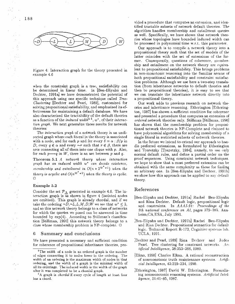
·1 188

, I

., . I

I

B

Figure 4: Interaction graph for the theory presented in example 4.6

when the constraint graph is a tree, satisfiability can be determined in linear time. In [Ben-Eliyahu and Dechter, 1991a] we have demonstrated the potential of this approach using one specific technique called Tree­Clustering [Dechter and Pearl, 1989], customized for solving propositional satisfiability, and emphasized its ef­fectiveness for maintaining a default database. We have also characterized the tractability of the default theories as a function of the induced width4 5 , w•, of their interac­tion graph. We next generalize those results for network theories:

The interaction graph of a network theory is an undi­rected graph where each literal in the theory is associated with a node, and for each p and for every fl= a : /3/ p in D, every q E a and every -r such that r E /3, there are arcs connecting all of them into one clique with p. Also, for each p- q in W, there is an arc between p and q.

Theorem 5.1 A network theory whose interaction graph has an induced width w• can decide existence, membership and entailment in O(n * 2w• +1 ) when the theory is acyclic and 0( n w• +2 ) when the theory is cyclic. 0

Example 5.2

Consider the set P ~ generated in example 4.6. The in­teraction graph is as shown in figure 4 (isolated nodes are omitted) . This graph is already chordal, and if we take the ordering -,D,-,L ,L,M,D,W we see that w• $ 3, and so this network theory belongs to a class of networks for which the queries we posed can be answered in time bounded by exp(4). According to Stillman's classifica­tion [Stillman, 1990) this network theory belongs to a class whose membership problem is NP-complete. D

6 Summary and conclusions

We have presented a necessary and sufficient condition for coherence of propositional inheritance theories , pro-

4The width of a node in an ordered graph is the number of edges connecting it to nodes lower in the ordering. The width of an ordering is the maximum width of nodes in that ordering, and the width of a graph is the minimal width of all its orderings. The induced width is the width of the graph after it was completed to be a chordal graph.

5 A graph is chordal if every cycle of length at least four has a chord.

vided a procedure that computes an extension, and iden­tified tractable subsets of network default theories. The algorithm handles membership and entailment 4ueries as well . Specifically, we have shown that network theo­ries whose topologies have bounded induced width can be processed in polynomial time w .r. t . this parameter.

Our approach is to compile a network theory into a propositional theory such that the set of models of the latter coincides with the set of extensions of the for­mer. Consequently, questions of coherence, member­ship and entailment on the network theory are equiva­lent to propositional satisfiability. This brings problems in non-monotonic reasoning into the familiar arenas of both propositional satisfiability and constraint satisfac­tion problems. Although we use here a two-step transla­tion (from inheritance networks to default theories and then to propositional theories), it is easy to see that. we can translate the inheritance network directly into a propositional theory.

Our work adds to previous research on network the­ories and inheritance reasoning. Etherington [Ethering­ton, 1987) has shown a sufficient condition for coherence and presented a procedure that computes an extension of ordered network theories only. Stillman [Stillman, 1990] has shown that the membership problem for proposi­tional network theories is NP-Complete and claimed to have polynomial algorithms for solving membership of a single literal in restricted subsets of network theories .

In the future we intend to extend our approach to han­dle preferred extensions, as formulated by Etherington and Touretzky [Touretzky, 1984], namely, to use only normal default rules, and define a partial order on the proof sequences. Using constraint network techniques, we hope to show that a most preferred extension can be obtained with the same complexity as those for findin15 an arbitrary one. In [Ben-Eliyahu and Dechter, l991bJ we show how this approach can be app lied to any defau lt. theory.

References

[Ben-Eliyahu and Dechter, 1991a] Rachel Ben-Eliyahu and Rina Dechter. Default logic, propositional logic and constraints. In AAAI-91: Proceedings of the 9th national conference on Al, pages 379-385, Ana­heim,CA,USA, July 1991.

[Ben-Eliyahu and Dechter, 1991b] Rachel Ben-Eliyahu and Rina Dechter. Propositional semantics for default. logic. Technical Report R-172, Cognitive systems lab. UCLA, 1991.

[Dechter and Pearl, 1989] Rina Dechter and Judea Pearl. Tree clustering for constraint networks. Ar­tificial Intelligence, 38:353-366, 1989.

[Elkan, 1990) Charles Elkan. A rational reconstruction of nonmonotonic truth maintenance systems. A rtifi­cial Intelligence , 43:219-234, 1990.

[Etherington, 1987] David W. Etherington. Formaliz­ing nonmonotonic reasoning systems. Artificial Int el­ligence, 31:41- 85, 1987.

[Gelfond and Lifschitz, 1990) M. Gelfond and V. Lifs­chitz. Logic programs with classical negation. In The 7th international conference on Logic Programming, pages 579-597, Jerusalem,Israel, June 1990.

[Kautz and Selman, 1991) Henry A. Kautz and Bart Selman. Hard problems for simple default logics. Ar­tificial Intelligence, 49:243- 279, 1991.

[Reiter and de Kleer, 1987) Raymond Reiter and Johan de Kleer. Foundations of assumption-based truth maintenance systems: Preliminary report . In AAAI-87: Proceddings of the national conference on AI, pages 183-188, Seattle,WA, July 1987.

[Reiter, 1980] Raymond Reiter. A logic for default rea­soning. Artificial Intelligence, 13:81-132, 1980.

[Stillman, 1990) Jonathan Stillman. It's not my default : The complexity of membership problems in restricted propositional default logics. In AAAI-90: Proceedings of the 8th national conference on artificial intelligence, pages 571- 578, Boston,MA, 1990.

[Touretzky, 1984) David S. Touretzky. Implicit order­ing of defaults in inheritance systems. In AAAI-84: Proceedings of the national conference on artificial in­telligence, pages 322-325, Austin,TX, 1984.

1 8 9

190

Decision-theoretic defaults

David Poole Department of Computer Science,

University of British Columbia, Vancouver, B.C., Canada V6T 1Z2

email: poole@cs.ubc.ca

Abstract

This paper considers defaults as summaries of decision-theoretic deliberations. We investigate the idea that the default e -+ a means that a is the optimal action based on all we know ( con­tingently) being e. It is shown how this notion of'a default is nonmonotonic and has a prefer­ence for more specific defaults. It has the ad­vantage of defaults can, in principle, be derived from lower level concepts. We thus have a ra­tional basis for determining whether a default is correct or not. One special case considered is where the action is whether to accept some proposition as true, accept it as false or nei­ther. This is needed to allow for conclusions to be used as premises in other defaults. It is shown that when the gain in utility of ac­cepting a proposition depends only only on the truth of the proposition, then the acceptance of q based on evidence e depends only on whether P(qje) exceeds a threshold that is a function of the utilities for accepting q. We also give a bound on the loss (in utility terms) of using an accepted proposition in another derivation.

1 Introduction

In AI, formal default reasoning started off as a spin off from logic [Reiter, 1980; McCarthy, 1980; McDer­mott and Doyle, 1980]. Logic is a normative theory of correct reasoning; the hope was that by adding in a " t . " . nonmono omc component, a normative theory of rea-soning where we jump to conclusions could be derived. Probability theory on the other hand started off as a normative theory of reasoning under uncertainty [Jef­freys, 1961], but is very quantitative in nature. Recently qualitative versions of probability theory have been pro­posed for default reasoning [Pearl, 1989; Neufeld, 1989; Bacchus, 1989]. One problem with all of these pro­posals (with some notable exceptions [Neufeld 1989· Bacchus, 1989]) is that we cannot "take the se~antic~ seriously"; there is no way to use the semantics to de­cide whether some default is correct or not. When we do take the semantics seriously it is not so obvious that the default statements say what we actually want to say.

1.1 Defaults and utilities

What one is prepared to say "yes" to depends on both utility and probabilistic information (Doyle [1989] argues this most strongly; see section 6.1).

If one is playing a game like "trivial pursuit" (where there is no penalty for saying something wrong over the penalty for saying nothing), it is better to have a wild guess at something than to say nothing. If one is in court acting as an expert witness, then one should only say what one is sure of; witnesses don't want to be caught out and have their credibility ruined. What one assents to, and so what defaults one uses, is very dependent on the situation and the utilities involved.

If one is in a closed room full of mixes of birds and someone opens up some windows high up in the room, then what one believes about the prototypical bird in ~he room changes as the proportion of the flying birds m the room changes1. At the start we may believe that the prototypical default bird in the room flies, but as the po~ulation of the birds change, after half an hour we may beheve that the prototypical bird in the room does not fly. Thus probabilistic information (information about proportions of populations with certain properties) does affect the defaults we make.

In this paper we consider a formulation of defaults that takes probability and utility into consideration.

1.2 The Proposal

Other people have observed that utilities have something to do with default reasoning [Shoham, 1987; Loui, 1990; Doyle, 1989; Kadie, 1988]. In this paper we take this re­lationship seriously and treat defaults as decision theory summaries.

A default e-+ A a means that a is the best decision out of those decisions in A if all you know is e. Note that the conclusion of a default is an action, and not a proposition as in most default frameworks (but see section 4).

The default "if you are in Vancouver in November ' carry an umbrella" , is of this type of a default that has

an action as a conclusion and propositions as premises. This is represented as

in_Vancouver A is..November-+ carry_umbrella

1 This example is due to Alan Mackworth (personal communication)

The main feature of this framework are: • We develop a meaning for defaults and inherit a

calculus (albeit very weak) for reasoning with these defaults that is sound with respect to the semantics.

• We can take the semantics seriously, and argue whether or not some default is true or not. More­over, it can be argued that these default statements are the sort of statements that correspond to every­day defaults.

• This is useful in its own right as a summary of what actions should be taken based on certain evidence. For example, in some implementations of influence diagrams (those that evaluate the diagram inde­pendently of any particular observations) [Shachter, 1986], the output is a contingency table of the out­put for all tuples of possible observations. One of the motivations for this paper was to allow for a more compact representation of the decisions based on different combinations of observations.

• Building on a decision theoretic base, we develop the notion of approximate reasoning, where we can have a measure on the cost of making a mistake. This is useful when we want to develop a theory of fast, but approximate reasoning.

In section 4 we consider the special case of where the actions are to accept some proposition, to accept its negation or to accept neither. This is special as it allows us to use the conclusion of the default as a premise for more inference. We analyse the possible costs of making this unsound but often reasonable rule.

2 Background 2.1 Probability We use a standard definition of conditional Bayesian probability (e.g., [Jeffreys, 1961]), where P(al/3) is a function from two propositions into the interval (0, 1], where f3 'I. false. We use the formulation based on the three axioms:

1. P(x lx) = 1

2. P(--.x ly) = 1 - P(x jy) 3. P(x /\ yjz) = P(x jy /\ z ) x P(y lz) The following lemma can be easily proven from the

axioms and is used in this paper:

Lemma 2.1 P(x lz) = P(x ly /1. z) x P(yj z ) + P(xj--.y /1. z) x P(--.y jz )

We use the symbol ::} for normal logical (material) implication. Lemma 2.2 if y =} z then P(x jy /\ z) = P(xly).

2.2 Classical decision theory

Under classical Bayesian decision theory ( e.g., [Raiffa, 1968]), we assume that there is a subjective utility func­tion, µ( a, w) of the utility of action a if the world is w.

The expected utility of action a given evidence e, t' (a,e) is given by

t'(a,e) = L µ(a,w) x P(wle) w

This is the utility of a averaged over all possible worlds, weighted by their probability.

3 Decision-theoretic defaults If e is a formula in the propositional calculus, and A = { a1 , a2 , ... } is a set of possible alternate actions ( the possible actions being primitive), and a E A, we write

if t'(a,e) = max£(a;,e).

a;EA

In other words, e -+ A a if, &iven all that we know ( contingently - see [Poole, 1991]) is e, a is the action in A that maximises expected utility.

3.1 Nonmonotonicity

The following example shows how the meaning of de­faults can allow us to derive defaults from lower level constructs. Note that, in general the user would not provide the probability and utility, but only provide the default. Because we have a formal definition of the truth of a default, we can argue about whether some default is reasonable (based on whether the underlying proba­bilities and defaults are reasonable). This example also shows the notion of defaults is nonmonotonic and shows how we have a preference for more specific defaults.

Example 3.1 Suppose we have the possible actions

A = { say.flies, say.not.flies, say.nothing}

and the following underlying utility and probability in­formation:

µ( say. / lies, flies) = 100 µ( say.flies, --.J lies) = - 200

µ( say.not./ lies, flies) = - 200

µ( say.not./ lies, --.J lies) = 100 µ( say.nothing, flies) = 0

µ( say.nothing, --.J lies) = 0

P(f lies lbird) = 0.9

P(flieslemu) = 0.001 P(bird jemu) = 1

Given bird we can derive the following expected utili­ties

£( say. / lies, bird) = µ(say . flies, flies) x P(flies lbird)

+µ( say./ lies, --.J lies) x P(--.J lieslbird) = 100 X 0.9 - 200 X 0.1

= 70 £( say.not./ lies, bird)

= µ( say.not. / lies, flies) x P(f lies lbird) +µ( say.not./ lies, --.J lies) x P(--.J liesjbird)

= - 200 X 0.9 + 100 X 0.1

= - 170 £( say.nothing, bird)

191

192

-1

= µ( say_nothing, flies) x P(f lies lbird)

+µ( say_nothing, -.J lies) x P(-.J lies lbird)

= 0

Thus we can derive the default

bird - A say_/ lies

Similarly if we were given emu, we can compute the ex­pected utility as:

£( say_/ lies, emu ) = -199.9 £ (say_not_flies, emu ) = 99.7

£( say_nothing, emu ) = 0

Thus we can derive the default

emu - A say_not_f lies

If we are given bird I\ emu we can use lemma 2.2 to show that the same deviation works as when we are given just emu and so we have:

bird I\ emu - A say_not_f lies

There are two things that can be derived from this example

nonmonotonicity When we learnt new information, namely that the individual was an emu as well as a bird, we no longer derived the conclusion say_flies, but rather derived the conclusion say_not_f lies. We thus change our minds when presented with differ­ent information.

specificity If we know that emus are birds, when we have both emu and bird, we make the same conclu­sion that we would using just emu. This preference for more specific defaults is true in general (section 3.2).

3.2 Specificity

One of the features of defaults that is important is the fact that more specific defaults should over-ride more general defaults. If we have x => y, then knowing x is more specific knowledge than knowing y. When we have the defaults x - A a and y - A b, then when given x I\ y we should conclude, by specificity, a. The following proposition establishes this:

Proposition 3.2 If x => y and x -A a then x /\ y -A a.

The proof of this and other propositions appears in Appendix A.

This result should not be too surprising, as the prefer­ence for more specific knowledge is common to the P.rob­abilistic formulations of defaults (see [Pearl, 19891) , as opposed to the logical formulations of defaults.

3.3 Ignoring Irrelevance If we have some condition c such that we make the same decision whether or not c is true, then we will make that decision even if we did not know the truth of c.

Proposition 3.3 The following is valid inference:

e/\c-Aa e I\ -.c -A a

e-A a

Thus if would make the same decision if c is true or false, then we can ignore the value of c in our defaults. What is important here is that we can derive conse­quences of our defaults based on the underlying defi­nition.

3.4 Disjunction

We cannot do arbitrary reasoning by cases. For example the disjunction rule of Pearl [1989]

e1 V e2 -A a

is not valid in general. It is however valid when e1 and e2 either imply each other or are inconsistent. Accepting this rule would lead us to Simpson's paradox [Neufeld and Horton, 1990].

3.5 Restricting the choices

Sometimes we may have fewer choices to make than at other times. The following proposition shows that if we do not eliminate the best choice, we can restrict the choices available without affecting the default.

Proposition 3.4 If e - A a and B ~ A such that a E B then e -Ba.

We can use the following lemma to split the set of possible alternatives.

Proposition 3.5 If e - A a and e - B b then either e - AUB a or e - AUB b

In the rest of the paper we assume that the set of choices of actions is fixed, and omit the subscript to -.

4 Acceptance Assumption

The preceding section considered the case when the con­clusion of a default was an action. Often in default rea­soning, we want to use a default to conclude that some proposition is true, and then use that proposition in fur­ther reasoning.

Jon Doyle has previously propounded the idea that we expand on:

"... we wish to use rationality as a standard for adopting assumptions by saying that an as­sumption should be adopted if the expected utility of holding it exceeds the expected utility of not holding it." [Doyle, 1989, p. 5]

In this section we show how to relate the action that is a conclusion of a default to the acceptance of the truth of a proposition. We consider the acceptance of a proposi­tion as a decision like another decision. For a proposition z there are three alternate decisions that could be made:

• zt is the decision to accept proposition z as true.

• zl is the decision to accept z as false.

• zu is the decision to neither accept z nor -,z.

For each proposition we make the decision of whether to accept it as true, to accept it as false or to make no commitment.

Example 4.1 We write the decision to accept flies as true if the individual under consideration is a bird as

bird - f lies1

This would correspond to the default in example 3.1, but the action is to accept the proposition flies, rather than the action to say something. Similarly the default that injured birds do not fly, can be written:

bird A injured -+ f lie sf

This says that if all you know about some individual is that the individual is an injured bird, that it is better to assume that it does not fly, than being uncommitted about the flying ability of the individual or assuming that it does fly.

We also allow for a default to conclude that we should not assume anything about the flying ability of young birds:

bird A young -+ f liesu

Note that we only have a two valued logic ( classical probability theory is based on every proposition being true or false in each possible world [Jeffreys, 1961]), but we have three possible actions that we can do with re­spect to a proposition. We assume here that it is never a good policy to assume a proposition and its negation.

Assumption 4.2 We assume the following inequalities:

µ(zllz) < µ(zulz) < µ(ztlz)

µ(ztl-,z) < µ(zul-,z) < µ(zll-,z) That is it is better to guess correctly than to be non­committal. And it is better to be non-committal than guessing wrongly2 •

The second assumption that we make is that the util­ities of different propositions are in some sense indepen­dent. We can treat the gain in accepting proposition z as not affected by the truth of other propositions.

Assumption 4.3 The change in utility of accepting z or accepting -,z or accepting neither in a world w de­pends only on the truth of z in w.

That is, if w1 and w2 are two worlds that agree on the truth of z then

µ( zr,w1)- µ( z8,w1) = µ( zr,w2)- µ( z8 ,w2)

where {r,s} C {t,u,f}. This assumption means that we only have to consider

the gain in making the correct decision and the loss in making an incorrect decision.

Definition 4.4 If p is an atomic proposition we use the following notational schema where r and s denote differ­ent elements of { t, f, u }, and <T is a sign ( one of+ or -i) such that <Tp is p if <T is + and <Tp is -ip is <T is -i. We define

rAs(<Tp) = µ(p8,w) - µ(pr,w) where w is a world in which <Tp is true. This schema, representing 12 different formulae, denotes the change in utility made what changing our action from r to s.

2 Analogous results to the ones below hold when the above constraints are violated - the arithmetic is slightly changed.

For example, f At(z) is µ(zt, w) - µ(zl, w), where z is true in w, which is the utility gained when we decide to commit to z over committing to -,z given that z is true.

uAf(-, z) is µ( zl,w) - µ( zu,w), where z is false in w, which is the utility gained when we decide to commit to -, z over not committing to the truth of z given that z is false.

Under assumption 4.2, f At(z), f Au(z) and uAt(z) are all positive. These all consist of the gain made by making a better guess given that z is true. Note also that

f At(z) = f Au(z) + uAt(z).

Thus 1.!lf(-,z), uAf(-,z) and 1Au(-,z) are all positive. All of the others are negative, using the equality

rA8 (<Tz ) = - 8 Ar(<Tz)

Lemma 4.5 Fors and reach being one oft, u or f, the following holds:

£( z8,x) - £(zr,x) = rA 8 (z)xP(zlx)+rAs(-,z)xP(-,zlx)

4.1 Characterization of defaults

In this section we analyse when we can conclude a default based on the assumptions in the previous section. We first consider when one decision should be made over another decision. Lemma 4.6

t'(zt,x) ~ t'( zl,x)

if and only if

Lemma 4.7

if and only if

1.!lf(-,z) P( zlx) ~ f At(z ) + t.!lf(-,z)

tAu(-,z) P( zlx) > ----------­- uAt(z) + tAu(-,z)

The following theorem is a direct corollary of lemmata 4.6 and 4.7.

Theorem 4.8 x -+ zt if and only if

What is important to notice here is that the decision to accept z based on x is determined completely by a threshold on the probability P(zlx) and that the thresh­old is a function of the utilities of the acceptance of z.

We can carry out a similar analysis of Lemma 4.9

t'( zU,x) ~ t'( zl,x)

if and only if

1 93

194

. I

The following theorem is a direct corollary of lemmata 4.6, 4.7 and 4.9.

Theorem 4.10 x -+ zt iff

( tAf(-,z) tAu(-,z) )

P(zlx) ~ max f At(z) + tAf(-,z)' uAt(z) + tAu(-,z)

X-+ zf iff

P z x < mm . ( tAf(-,z) uAf(-,z) )

( I ) - f At(z) + tAf(-,z)' f Au(z) + uAf(-,z)

x-+ zu iff P(zlx) is between these two values .

Example 4.11 Suppose we have the following utilities

µ(pu,p) = µ(pu, ..,p) = 0

µ(pt, p) = µ(pf, -.p) = a

µ(pt,-.p) = µ(pf,p) = - b

a is the prize we get for guessing right. b is the price we pay if we are wrong; both a and b are positive.

We have:

tAf(-,z) = 0.5

f At(z) + tAf(-,z) tAu(-,z) b

= uAt(z) + tAu(-,z) a+b uAf(-,z) a

f A u(z) + uAf (-.z) = a+b

We have the following cases of acceptance:

a>b

q -+ pt if P(plq) ~ ~ 1

q -+ pf 1'f P( I ) < p q - 2

Here we would never decide on pu. We would expect to lose by being noncommittal.

a=b

q-+ pt if 1

P(plq) ~ 2 q-+ Pu

1 if P(plq) = -

2

q-+ pf if 1

P(plq) ~ 2

Here, when P(plq) = k, it doesn't matter which decision we make. They all have the same expected utility.

a<b

q-+ l if b

P(plq) ~ a+ b

q-+ pf if a

P(plq) ~ a+ b

q-+ Pu if a < P( I ) < b a+b- pq_a+b

If we are very conservative we would expect that b ~ a. In this case we have

b --:::::1 a+b

The algebra of thresholding probability here is the same as the system of Bacchus [1989], but where the actual value of the threshold depends on the utilities associated with the acceptance of the conclusion of the default.

5 Approximate Reasoning

One of the features of utility-based approach to default reasoning is the ability to have a notion of the cost of get­ting a wrong answer. We can thus talk precisely about a tradeoff of accuracy, and consider the cost of making assumptions. Consider the following rule ( called "con­traction" [Pearl, 1989]):

X-+ yt XI\ y-+ zt

X-+ Z

This rule says that if we can conclude y, and use y to conclude z then we can conclude z without using y. This rule says that we can use derived conclusions as lemmata for other conclusions. This is not a valid rule of inference in the decision-theoretic defaults [Bacchus, 1989]. This is because we do not know that y is true we have only decided that we should make it true.

Pearl [1989] argues that €-semantics (in which con­traction is a valid rule) is an idealisation. One of the main advantages of the decision-theoretic defaults is that we can measure the cost of our idealisation. With the decision-theoretic defaults we can consider how much we can lose by applying the above rule.

Proposition 5.1 The maximum that we can lose by fol­lowing the above rule is

(1 - th(y1)) x tAf(-,z)

where th(y1) is the threshold for accepting y, which is

· ( 1Af(-,z) tAu(-,z) )

th(y1

) = max f At(z) + tAf(-,z)' uA1(z) + tAu(-,z)

Example 5.2 Using the utilities of example 4.11, we find that the maximum we can lose is

= (1 - th(y1

)) x 1Af(-,z) a

-bx (a+b) a+

= a

Even if we are extremely conservative and have a large b value, the conservatism in the acceptance of y means that we cannot lose much when we accept z.

6 Comparison with other proposals

6.1 Doyle Doyle has also considered the role of utility and probabil­ity in default reasoning [Doyle, 1989]. This paper can be seen as following in the pioneering steps of [Doyle, 1989]

in incorporating rationality into reasoning. We go into much more detail in one case of the general framework outlined by Doyle.

Doyle [1990] motivates his rational belief revision in economic terms. However, unlike the defaults in this paper, the object level statements are not statements of preference in a utility sense. The utility is to suggest alternate definitions of belief revision. I would argue that the notion of utility of beliefs should be logically prior to the notion of rational belief revision. Once we have a notion of the utility of belief, we should be able to use this to develop a notion of rational belief revision.

Other work of Doyle [1985; 1989] has considered the problem of default reasoning as a problem of group de­cision making, and used the theory of group decision making for default reasoning. The group decision mak­ing and the individual decision making used in this pa­per are not incompatible ( unless we want to claim they are the same [Doyle and Wellman, 19891), and so these approaches should be seen as complementary to the ap­proach propounded here.

6.2 Shoham

Shoham [1987] has argued that we should take probabili­ties and utilities into account when considering defaults. Here we take this suggestion seriously and consider the normative theory of decision making as a starting point. He instead develops a general framework of nonmono­tonic reasoning based on ordering of interpretations. The system propounded here cannot be simply put into the framework developed by Shoham ( one of the reasons is that we have automatic specificity, which one can show cannot be in any system that treats all logically equiva­lent formulae as equivalent [Poole, 1991]).

6.3 Loui

Loui [1990] has also proposed a mix between decision theory and defeasible reasoning. He has, however, sug­gested the opposite mix, namely using a form of defea­sible reasoning for decision making. His motivation is very different to the motivation of this paper; it is an intriguing idea to consider whether the default system propounded here could be used as the basis for the ar­gument system in Loui's proposal.

6.4 Bacchus

Bacchus [1989] has investigated the logic of thresholding conditional probability. All of the results of his theory can be transferred to the system in this paper. We com­plement Bacchus' work in that we show how straight­forward decision-theoretic concerns lead us to threshold­ing probability.

Rather than having a constant threshold for accep­tance, we have a different threshold for each proposition. While this is not inconsistent with Bacchus's results, it is interesting that we can determine exactly what the threshold should depend on. This is because we can an­swer the question of where the thresholds come from.

In Bacchus's system, all one can say about such rules as contraction ( section 5) is that they are unsound with respect to the thresholding semantics. In the system

outlined in this paper we can answer the question of how much we can lose by using these idealised rules of inference. and look at the utility of using conclusions, even if they may be mistaken.

7 Conclusion

In this paper we considered a simple idea; namely that defaults provide summaries of possible decisions that has already taken utilities and probabilities into considera­tions. This allows for a definition of default for which we can take the meaning seriously. I would argue that the default "birds fly" really means that if all you know about some individual is a bird, then it is good policy to assume that the individual can fly. Rather than us­ing decision theory directly for nonmonotonic reasoning [Kadie, 1988], this paper has explored only having the summaries of good decisions as defaults.

The main result was to show that under the assump­tion that the utility of the choice of whether to accept a proposition depends only on the truth of the proposi­tion ( assumption 4.3), the acceptance depends on thresh­olds of conditional probability. Thus we get to the same system that Bacchus [1989] proposed. We have the ad­vantage that we can derive the threshold for acceptance from utility considerations. This is one of the few pro­posals that can use the idea of the cost of an incorrect conclusion.

The resulting calculus is very weak. Further work can be carried out in incorporating independence assump­tions, and in making assumption 4.3 more realistic. As­sumption 4.3 is interesting as an idealisation, but is not practical. In practice the importance of a piece of infor­mation critically depends on what other information is true.

A Proofs

Proposition 3.2 If x ~ y and x ..... a then x /\ y ..... a.

Proof: If x ~ y then P(y lx) = 1.

&(a;,x/\y)

= Lµ(a;,w)xP(w lx/\y) w

= L µ(a;, w) x P(wlx) (by lemma 2.2) w

= &(a;,x)

The result follows immediately. D

Proposition 3.3 The following is valid inference:

e/\c ..... Aa

e /\ -,c ..... A a e ..... A a

Proof: Using lemma 2.1, we have

P(wle) = P(wle /\ c) x P(cle)

+P(wle /\ -,c) x P(-,cle) £(a;, e)

19 5

196

w

= P (cle) Lµ (ai, w) x P(wle I\ c) w

+P{-icle) Lµ (ai, w) x P(wle I\ -ic) w

= P (cle)£ (ai,e I\ c) + P (-icle)£ (ai,e /\ -ic)

We know e I\ c -+ a and e I\ -ic -+ a, so for each ai E A,

given£(a,e /\ c) ~ £ (a;,e /\ c)

and£{a,e /\ -ic) ~ £ (ai,e /\ -ic) then P(cle)£(a, e ,\ c) +

P (-icle)£ {a,e/\-ic) ~ P(cle)£(a;,e /\ c) + P (-,cle)£(a;,e /\ -ic)

so £(a,e ) ~ £(ai,e )

D

Lemma 4.5 For s and r each being one of t, u or f, the following holds:

£(z8, x )-£(zr, x ) = r L~.8 (z) xP(zlx)+r A 8 (-iz ) xP(-,zlx )

Proof:

D

£(z8,x ) - £(zr,x )

= Lµ (z8,w) x P(wlx ) - Lµ (zr,w) x P(wlx )

= w w

w:z true in w

(µ(z8,w) - µ(zr,w)) x P(wlx )

(µ(z",w) - µ(zr,w)) x P(wlx ) + w:z false in w

w:z true in w

P (wlx)

P (wlx ) w:z false in w

= r A 8 (z) X P(zlx ) + r A 8 (z) X P(-,z lx )

Lemma 4.6 £(z',x) ~ £(zl,x )

if and only if

tAf (-,z) P (zlx ) ~ f At (z) + tAf (-,z )

Proof: The following sequence of inequalities are all equivalent:

D

£(z',x ) ~ £(zl,x )

£(z',x)-£(zl,x) ~ 0

f At (z) x P(zlx ) - tAf (-,z ) x P(-,zlx ) ~ 0

f At (z) x P(zlx ) ~ tAf (-,z ) x {1- P(zlx )) (f At (z) + tAf (-,z )) x P(zlx ) ~ tAf (-,z )

tAf(-,z) P(zlx ) ~ f At (z) + tAf (-,z)

The proofs of lemmata 4. 7 and 4.9 are analogous to the proof of lemma 4.6, and are omitted.

Proposition 5.1 The maximum that we can lose by following the rule of contraction is

{1- th(yt )) x tAf (-,z )

where th(yt ) is the threshold for accepting y, which is

t _ ( tAf (-,z ) tAu (-,z) ) th(y ) - max f At (z) + tAf (-,z )' uAt (z ) + tAu (-,z)

Proof: Suppose we have x -+ yt and x I\ y -+ zt. The maximum we can lose by using the rule x -+ zt is given by how much we would gain by doing one of the other two actions. This is

max (£(zU,x ) -£(z',x ),£(zl,x ) - £(z',x ))

For s being either of u or f, we can derive

£(z8,x) - £(zt,x) = - 8 A'{z) X P(z lx) + tAs(-,z) X (1- P(z lx)) = tA8 (-,z ) - (8 At (z) + tAs (-,z)) X P (zlx )

P (zlx ) = P(zlx I\ y) x P(ylx ) + P (zlx I\ -iy ) x P (-,y lx) > P(zlx I\ y) x P(ylx )

( tAs (-,z) )

~ sAt (z ) + tAs (-,z ) X th(yt )

£(z8,x ) -£(z',x ) ~ tA 8 (-iz) - (8 At (z) + tAs (..,z)) X

( tA" (-,z) )

sAt (z) + tAs (-,z) X th(yt )

= tA 8 (-iz)- tAs (-,z) X th(yt) = tAs{-,z) X {1- th(yt ))

So that maximum that we can lose is

max (' Af (-,z) x (1- th(yt )) , tAu (-,z) x (1- th(yt )))

which, under assumption 4.2 is tAf (-,z ) x (1- th(y1) ) .

D

Acknowledgements

This research was supported under NSERC grant OG­P0044121, and under Project B5 of the Institute for Robotics and Intelligent Systems.

References

[Bacchus, 1989] F. Bacchus. A modest, but semanti­cally well founded, inheritance reasoner. In Proc. 11th International Joint Con/. on Artificial Intelligence, pages 1104-1109, Detroit, August 1989.

[Doyle and Wellman, 1989] J. Doyle and M. P. Well­man. Impediments to universal preference-based de­fault theories. In R. Reiter R. J. Brachman, H. J. Levesque, editor, Proc. First International Con/. on Principles of Knowledge Representation and Rea­soning, pages 94-102, Toronto, May 1989.

[Doyle, 1985] J. Doyle. Reasoned assumptions and pareto optimality. In Proc. 9th International Joint Con/. on Artificial Intelligence, pages 87- 90, Los An­geles, August 1985.

[Doyle, 1989] J. Doyle. Constructive belief and rational representation. Computational Intelligence, 5(1):1- 11, February 1989.

[Doyle, 1990] J. Doyle. Rational belief revision. In Preprints of Third International Workshop on Non­monotonic Reasoning, Lake Tahoe, CA, May 1990.

[Jeffreys, 1961] H. Jeffreys. Theory of probability. Ox­ford University Press, Oxford, third edition, 1961.

[Kadie, 1988] C. M. Kadie. Rational nonmonotonic reaoning. In Proc. Fourth Workshop on Uncertainty in Artificial Intelligence, pages 197-204, University of Minnesota, August 1988.

[Loui, 1990] R. P. Loui. Defeasible decisions: · what the proposal is and isn't. In M. Henrion et. al., editor, Uncertainty in Artificial Intelligence 5, pages 99-116. North Holland, 1990.

[McCarthy, 1980] J . McCarthy. Circumscription- a form of non-monotonic reasoning. Artificial Intelli­gence, 13(1,2):27- 39, 1980.

[McDermott and Doyle, 1980] D. McDermott and J. Doyle. Non-monotonic logic I. Artificial In­telligence, 13:41- 72, 1980.

[Neufeld and Horton, 1990] E. Neufeld and J . D. Hor­ton. Conditioning on disjunctive knowledge: Simp­son's paradox in default logic. In M. Henrion et. al., editor, Uncertain.ty in Artificial Intelligence 5, pages 117- 125, 1990.

[Neufeld, 1989] E. Neufeld. Defaults and probabili­ties; extensions and coherence. In H. J . Levesque R. J . Brachman and R. Reiter, editors, Proc. First International Con/. on Principles of Knowledge Rep­resentation and Reasoning, pages 312- 323, Toronto, May 1989.

[Pearl, 1989] J. Pearl. Probabilistic semantics for non­monotonic reasoning: A survey. In H. J . Levesque R. J . Brachman and R. Reiter, editors, Proc. First International Con/. on Principles of Knowledge Rep­resentation and Reasoning, pages 505- 516, Toronto, May 1989.

[Poole, 1991] D. Poole. The effect of knowledge on be­lief: conditioning, specificity and the lottery paradox in default reasoning. Artificial Intelligence, 49:281-307, 1991.

[Raiffa, 1968] H. Raiffa. Decision Analysis. Addison­Wesley, 1968.

[Reiter, 1980] R. Reiter. A logic for default reasoning. Artificial Intelligence, 13(1,2):81- 132, 1980.

[Shachter, 1986] R. D. Shachter. Evaluating influ-ence diagrams. Operations Research, 34(6):871- 882, November-December 1986.

[Shoham, 1987] Y. Shoham. Nonmonotonic logics: Meaning and utility. In Proc. 10th International Joint

Con/. on Artificial Intelligence, pages 388- 393, Milan, August 1987.

197

198

·, · 1

I

Hierarchical meta-logics for belief and provability: how we can do without modal logics *

Fausto Giunchiglia1•2 and Luciano Serafini1 Mechanized Reasoning Group

1 IRST, Povo, 38050 Trento, Italy 2DIST, University of Genoa, Via Opera Pia llA, Genova, Italy

fausto@irst.it, serafini@irst.it phone: +39 461 814440, fax: +39 461 810851

Abstract

MultiLanguage systems (ML systems) are for­mal systems allowing the use of multiple dis­tinct logical languages. In this paper we intro­duce a class of ML systems which use a hierar­chy of metatheories, each with a first order lan­guage containing names for the language below, and propose them as an alternative to modal logics. The motivations of our proposal are technical and epistemological. From a technical point of view, we prove, among other things, that modal logics can be embedded in the corresponding ML systems. Moreover, we show that ML sys­tems have properties not holding for modal log­ics and argue that these properties are justi­fied by our intuitions. We motivate our claim by studying how they can be used in the rep­resentation of beliefs (more generally, propo­sitional attitudes) and provability, two areas where modal logics have been extensively used.

1 Introduction and motivations

It has been argued that knowledge should be struc­tured into sets of facts or theories ( often called "con­texts"); some of the many examples are [Giunchiglia and Weyhrauch, 1988; Giunchiglia, 1992a; Weyhrauch, 1980; McCarthy, 1990; Kim and Kowalski, 1990]. In [Giunchiglia, 1991; Giunchiglia and Serafini, 1991a] the authors take a further step and introduce a new gen­eral kind of formal systems allowing multiple distinct languages and call them Multi-Language systems (ML systems). In [Giunchiglia, 1991] it is argued, in fact, that providing each theory with its own language allows us to give a natural and elegant proof theoretic account of multi-contextual reasoning and, also, extra flexibility which can be exploited in the representation of many phenomena.

In this paper we focus on a particular class of ML sys­tems which allow a hierarchy of metatheories, each using a first order language containing names for the language

•This work has been done as part of the project "MAIA", Advanced Model of Artificial Intelligence, under development at IRST.

below and propose them as an alternative to modal log­ics. We show how modal systems can be embedded in the corresponding ML systems by providing an equivalence result between their provability relations. Moreover, we prove that the ML systems we consider have further properties, not holding in modal logic, and argue that these properties are grounded into our intuitions. To justify our claim WP study how ML systems can be use_d in the representation of beliefs (more generally, proposi­tional attitudes) and provability, two areas where modal logics have been extensively used; [J .Y. Halpern, 1985] and [Boolos, 1979] are some of the many references on the use of modal logics respectively on the first and the second topic.

One of our main interests is to provide foundations to the implementation of "intelligent" reasoning sys­tems. The issue of mechanizibility and of naturalness of the interaction with the implemented system plays a central role in our research. The ideas described here have been incorporated into a system, called GETFOL, which gives the user the ability to define arbitrary ML systems (GETFOL is a total re-implementation/extension of the FOL system [Weyhrauch, 1980; Giunchiglia and Weyhrauch, 1991]).

The paper is strnctured as follows. Section 2 gives a short description of some basic notions concerning ML systems (but see [Giunchiglia, 1991] for a much longer presentation) . Section 3 introduces the class Mn, the Mn system MBK for the representation of propositio~al attitudes and the Mn system MK for the representat1011 of provability. Section 4 proves and discusses the main technical results about MBK and MK. Finally section 5 shows how Mn systems can be extended to capture var­ious modal logics. Proofs are skipped, for a complete treatment of the t,!chnical issues see [Giunchiglia and Serafini, 1991b].

2 ML systems

The goal of this section is to give a formalizatio!' of t!1e idea of system with multiple languages. A detailed dis­cussion about the d,!finitions concerning ML systems can be found in [Giunchiglia, 1991].

An axiomatic formal system S is usually described as a triple consisting of a language L, a set of axioms n~L and a set of inference rules Ll, i.e., S = (L, n, Ll).

The generalization we consider here is to take many lan­guages and many sets of axioms while keeping one set of inference rules. We thus have the following definition of multi-language system:

Definition 2.1 (Multi-Language System) Let I be a set of indices, { L1 her, a family of languages and {D1her a family of sets of wffs such that D;<;L;. A Multi-Language Formal System (ML system) MS is a triple ({L;}ier,{D;}ier,~) where {L;};er is the Family of Languages, {D;}iEI is the Family of sets of Axioms and ~ is the Deductive machinery of MS.

If A is a wff of a language L, we say that A is an L­wff. Each language L 1 is associated with its theory ( de­fined as the set of L;-wffs which can be proved by apply­ing the deduction machinery to the axioms). What can be derived is bound by language: certain formulas (like the conjunction of two theorems in two distinct theories) cannot be derived simply because there is no language in which they can be expressed .

Even if definition 2.1 is more general, allowing arbi­trary formal languages and deductive machinery, in this paper ( and in most of the work done so far), we con­centrate on first order languages and adopt a suitable modification of the natural deduction formalism, nota­tion and terminology defined in [Prawitz, 1965]. More­over, as we want to make effective use of the multiple languages, we define the inference rules in a way to take into account the language the wffs are extracted from. We write (A, i) to mean A and that A is a L;-wff. The deduction machinery ~' is therefore defined as a set of inference rules, written as:

(Ai , i1) (An , in ) ---------- l (A, i)

(1)

or as :

[(Bi, ii)] [(Bm, Jm)] (An+l, in+1), , .(An+m, in+m) (A , i)

8

(2) Picture (2) represents a rule 8 discharging the assump­tions (B1, }1), . . . , (Bm , Jm) [Prawitz, 1965] . Notice that in general, inference rules have premises and conclu­sions belonging to different languages. The rules whose premises and conclusions belong to the same language L; are called L;-rules, the others bridge rules [Giunchiglia, 1991]. L;-rules allow to draw consequences inside a the­ory while bridge rules allow to export results from one theory to another. One example of L;-rule for a theory i is modus ponens

(A-B, i) (A, i)

(B, i)

one example of bridge rule between the theories i, j and the theory k is multicontextual modus ponens [Giunchiglia, 1992a]

(A-B, i) (A, j) (B, k)

The meaning of the two rules is very different. The first allows us to derive B inside the theory i just because we

199

•("A") •("A'')

_____ ---- -----! n'"'-- -----f n.,., _____ _ A A

Figure 1: The family Mn

have derived A - B and A in the same theory. Thus, for instance, if we take the theory i to represent the beliefs of an agent a;, this means providing the agent a; with the ability of using modus ponens. Multicontextual modus ponens allows us to derive B in the theory k just because we have derived A - B in the theory i and A in the theory j. If we take the theories i, j, k to represent the beliefs of the ag•mts a1 , ai, ak, this means that ak will be able to take B as known, not because he has derived it, but because this is the result of the interaction of the results derived by a; and ai . The assertion of B in k is not the result of a deduction in k but, rather the result of the "propagation" of reasoning from i, j into k. ( [ Giunchiglia, 1992a] describes these issues in more detail.)

Deductions are trees of wffs built starting from a finite number of assumptions and axioms, possibly belonging to distinct languages, and applying a finite number of in­ference rules. Any deduction can be seen as composed of subdeductions in di8tinct languages, obtained by repeated applications of L;-rnles, any two or more subdeductions being concatenated hy one or more applications of bridge rules.

3 The class J'vt'R..

Informally, Mn systems have the following properties:

(i) the languages are ordered in a hierarchy;

(ii) each language in the hierarchy has names for the wffs of the levd below;

(iii) any two adjacent languages in the hierarchy, say M and O, are linked only by two bridge rules which are variations of the multi-language version of reflection up and reflection down ( as described in [Giunchiglia and Smaill, 19x9]) . In other words the bridge rules are of the form:

____.:.( A.....;,,_O-"-) _

(•("A"), AI) nup.

(•( "A") , M)

(A, 0)

where "•" is a unary predicate.

Figure 1 gives a graphical representation of the basic structure of the elements of Mn.

Each Mn system is a hierarchical meta-logic, in the sense that each pa ir of connected theories, 0 and M ,

200

I

satisfies the following conditions:

~ A if and only if ~ •("A") (3) . ~ • ("A-+B")-+(•("A" )-•("B")) (4)

which are the weakest conditions that guarantee the ob­ject/ meta relation between two theories.

In this section we present and discuss two important instances of Mn systems, that is MBK for the represen­tation of propositional attitudes and MK for the repre­sentation of metatheoretic theorem proving.

3.1 MBK: reasoning about propositional attitudes

MBK is the basic system for the representation of propo­sitional attitudes. To keep things simple we consider the single agent case. The generalization to the multi-agent case is straightforward.

The idea underlying the formalization of propositional attitudes is that there is an agent, let us call him a, who is acting in a world, and has both beliefs about this world, and beliefs about his own beliefs . For a proposi­tion A about the state of the world, Bl( "A") means that A itself is believed by a or, in other words, that A holds in a's view of the world; similarly Bl("Bl("A")") means that Bl("A") is believed by a, i.e. A holds in a's view of his beliefs of the world, and so on. In other words, a "sits on top" of his beliefs and is able to reason on the reification of his belief A, that is Bl( "A"), in a sort of "metaview" ofa believing A.

This process of reification can be iterated through a chain a metaviews; a's beliefs are thus the facts derived in a top theory which has a metaview, a metametaview, a meta .. . metaview of a's own beliefs.

To formalize the notion of belief in a multi-language framework we have a chain of theories, called views, where the theory above "sees" the theory below via re­flection principles which allow the derivation of Bl( "A") from A and viceversa (see figure 2). This chain has a top theory which is a's beliefs, that is, its basic beliefs about the world and his view of all the possible nestings of the belief predicate. In the case of the ideal reasoner, which we consider in the following, we need to have an infinitely descending chain and thus no bottom theory ( one more level of nesting of the belief predicate corresponds to one more theory in the chain, see figure 2).

As each theory is "above" an infinite chain and each level corresponds to a level of nesting of the belief pred­icate, all the languages in MBK must have the same expressibility, i.e. they must have the same notion of wellformedness.

To define MBK we need a way to index theories in the infinitely descending chain. We index the top theory with 0, the one below with 1 and so on.

In MBK the languages L(BO, are thus obtained from a propositional language L as follows:

Lo= L

Ln+l = Ln U {Bl("A"): A is an Li-wff}

L(BO = Unew Ln

Here L is the language used to express the basic facts about the world.

Bl("A") Bl( "A" )

_____ ---------}- n.,., -----{-- n'"·' __ _

A A

I

-----~------------------------------ --1 I I I ----------------------~

Figure 2: The system MBK

Definition 3.1 (MBK) Let L be a propositional lan­guage. Then MBK= ({Li}iew, {rli}iew, ~), is such that, for every i E w , L; = L(Bl), fii = 0 and il contains th e following rules:

((A, i)] (B, i)

...,.....----,- - [j {A-+B, i)

[(-,A, i)] ( .L, i) (A, i) .Li

(A, i + 1) (Bl("A"), i ) Rup i

(A, i) {A-+B, i) (B, i)

-+E;

(Bl("A" ),i} R. {A, i + 1) an .i

Restrictions: the Rup.i-rule can be app lied only if the index of every undischarged assumption (A, i) depends on, is lower than 01 · equal to i . .Li can be applied if A -is not of the fo rm .L.

The idea underlying the definition of MBK is that the only bridge rules arf' reflection up and down between any two adjacent theories and that any theory i has a set of inference rules which is complete for classical proposi­tional logic (this ensures that the i-th theory contains all the tautologies).

A lot of people in the AI and cognitive science commu­nity have argued in favour of this kind of "distributed" representation of bdiefs and deductions. ( Notice that in the multiagent case. instead of a hierarchy, we have a tree of theories. In this tree, each theory is above n theories, one for each agent; Pach of these n theories represents the beliefs of an agent as "seen" by the theory above them) . For instance Wilks [Wilks and Biem, 1979], in his work on belief ascription, speech acts and so on, advocates the use of distinct sPts of beliefs; Fauconnier [Fauconnier, 1985] has a mental space theory which uses environment­like entities; Dinsmore in [Dinsmore, 1991] formalizes

Th("A") Th("A")

_____ -----------l n.,.1 _________ ! n,., __

A A

Figure 3: The system MK

agents' beliefs by belief spaces, each of which .can con­tain further belief spaces for the formalization of the agents' nested beliefs. Konolige formalizes agents' nested beliefs using introspective machines [Konolige, 1984; Konolige, 1985], which are very similar to theories. Kim and Kowalski in [Kim and Kowalski, 1990] propose a very similar approach in the area of logic programming.

Notice that Perlis [Perlis, 1985] argues explicitly against the use of multiple hierarchical theories, the main argument being one of quantification. He argues, rightly, that we do not want to quantify over all the different lev­els. His point does not apply here as we are dealing with the propositional case; on the other hand, we argue that, even in the first order case, his observation does not rule out the use of multiple levels and, more generally, of multiple contexts. Even in the first order case we do not need to quantify over theories unless this is exactly the kind of reasoning we want to do. The basic intuition, underlying all our work, is that reasoning is always con­textual and that, therefore, all the arguments are im­plicitly bounded to the current context and to the con­texts it implicitly refers to (see also [Giunchiglia, 1992a; McCarthy, 1991]). We never quantify explicitly over con­texts unless we want to make the contextuality of rea­soning explicit.

3.2 MK: reasoning with metatheories

In metatheoretic reasoning, one usually starts with the object theory and then defines its metatheory, its metametatheory and so on. Analogously, in MK, the bottom theory is any object theory, the theory at level 1 is its metatheory, the theory at level 2 is its metametatheory and so on. Thus, if L is the propo­sitional language of the object theory, for any natural number i (i E w), Li is inductively defined as follows :

Lo = L

201 Li+t = Li U { Th( "A") : A is an Li-wff}

where: Th is an unary predicate and "A" is an individual constant (which acts as the name of A).

Definition 3.2 (MK) Let L be a propositional lan­guage. Then MK= ({Li}iEw, {Q}iew, ~), is such that, for every i E w, n, = 0 and ~ contains the following rules:

[(A, i)] (B, i) _.;...__.;,_ -+ I;

(A-+ B, i)

[ (-,A, i)] ( .l, i) (A, i) .li

(A, i) (A- B, i)

(B, i) -E;

(A, i) (Th("A"), i + 1) 'Rup.i

(Th("A"), i + 1) (A, i) Rdn.i

Restrictions: the 'Rup.i-rule can be applied only if the index of every undischarged assumption (A, i) depends on, is strictly greater than i. .li can be applied if A is not of the form .l.

Figure 3 gives a graphical representation of the struc­ture of MK.

Analogously to l\lBK, in MK reflection up and down between any two adjacent theories are the only two bridge rules and any theory i can prove all the tautolo­gies. Most of the in tuitions underlying MK are reported in [Giunchiglia and Serafini, 1991b].

3.3 Some notes about MK and MBK

MBK and MK are similar but different. Not least, they use different hierarchies of languages. The differences be­tween MBK and MK can be best summarized by point­ing out that in MK we have only one object theory and an infinite number of metatheories while in MBK we have one meta ... metatheory and an infinite number of object theories. These differences, which are substantial and seem motivated by our intuitions, do not seem for­malizable in modal logics. Our explanation of this fact is that, in modal logics, collapsing all the languages in one, one loses track of how, depending on the applica­tion, language is used in the hierarchy of nestings of the proof/belief predicate. Note that the union of all the languages in MK is the same as the union of all the lan­guages in MBK modulo the substitution of Th with Bl. Having a unique language has caused a certain degree of confusion between provability and belief; for instance in [Konolige, 1984] belief has been modeled as provabil­ity.

Some basic theorems in MBK and proofs are listed below. The proofs are examples of how deductions are constructed in MBK.

Proposition 3.1 For any wff A and B and any i E w, (i)-(iii) are theorems of MBK.

(i) (Bl("A-+B")-+(Bl("A") -+ Bl("B")) , i) (ii) (Bl(".l")-+Bl("A''), i)

202

·· I

f,.

{iii} (-.Bl("..L")-.(Bl("A") -.-.Bl("-.A")) , i)

Proof (i)

( ii)

(iii)

(Bl( "A-B"), i) (A -B, i+l) ndn.i

(Bl("A"), i)

( ndn.i

A, i + 1) -E;+1

(B, i + 1) Rup.i

(Bl( "B" ), i) (Bl("A") - Bl("B"), i) -I; ___ ...;.......;..._..;.__....;..._..;._...;... ___ - I;

(Bl( " A-B")- (Bl(" A")- Bl("B")), i)

(Bl( ".L" ), i) Rd -

( .L, i + 1) . n. I

(A, i + 1) 1;,+1 .

(Bl("A"), i) up.,

(Bl( " .L")- Bl("A"), i) -I;

(Bl( "A"), i) (Bl( "-.A"), i) (A, i + 1) Rdn.i (-.A, i + 1) Rdn., ..;._ __ ...;... ____ .;..._ __ .....;.. -E,+1

(.L, i + 1) -'------'- 'llup.i

(-.Bl(".L"), i) (Bl(".L") , i) --'--__;..---'-------'-...;...-"--..;.. -E;

(.L, i) (-.Bl("-.A"), i) .L;

-I; (Bl("A")--.Bl("-.A"), i)

--------------- -+I; (-.Bl(" .L" ) - ( Bl( "A")-+ -.Bl( "-.A" )), i)

Q .E.D. Under the obvious interpretation (read Bl("A") as

DA) the three theorems above hold also for modal K. In particular the translation of the first theorem is the ax­iom characterizing modal K (that is D(A-.B)-.(DA-. DB).

The wffs obtained by replacing Bl with Th in ( i), ( ii) and ( iii) of proposition 3.1 are theorems of MK as well . Their proofs can be obtained by replacing i with i + 2 ( and leaving i + 1 as it occurs) in the proof of the corresponding MBK theorems.

4 The main results about MBK

This and the following section describe the main tech­nical results for MBK. Unless explicitly stated the con­trary, all the theorems hold also for MK, modulo some obvious syntactic modifications.

Let L be a propositional language. We define the modal language L(D) as the minimal set of wffs built with the usual rules for the logical connectives plus the following rule: if A is a L(D)-wff then DA is a L(D)­wff. The modal system K is characterized by the axiom schema D(A-. B)-. (DA -. DB) and by the necessita­tion rule: if~ A then ~ DA. To carry out the proofs of the theorems listed in these pages, we have used Bull and Segerberg's version of modal K, as described in [Bull and Segerberg, 1984].

The mapping( .)* from L(D)-wffs to L(B0-wffs is then defined as follows:

(i) If A is a propositional constant then A• = A;

(ii) (. )* distributes over the propositional connectives;

(iii) (DA)*= Bl("A*") .

(.)* is an isomorphism with inverse, which we write(.)+. The first result i:;; a form of syntactic equivalence be­

tween provability in K and in MK.

Theorem 4.1 If A is an L(B0-wff then for any i E w , · f;,, 8 K (A, i), if and only if~ A+.

Corollary 4.1 (Consistency) For every i E w, ( ..L , i) is not a theorem in MBK.

Notice that in [Rivieres and Levesque, 1986], Des Riv­ieres and Levesque show how Montague and Thomason 's negative results [Montague, 1974; Thoma.son , 1980] can be avoided with a careful translation of modal logics into first order logics. Besides the differences in the motiva­tions, the main technical difference between the results stated by theorem 4.1 and corollary 4.1 and those de­scribed in [Rivieres and Levesque, 1986] is that they keep a unique language while we propose a hierarchy of dis­tinct, possibly different (as in MK) languages. [Attardi and Simi, 1991] describes another approach where reflec­tion rules are used still keeping consistency; the main technical difference with our work is, again , that they use a unique (amalgamated) language.

Theorem 4.1 does not mean that Kand MBK 's prov­ability and, more important, derivability relations can be put into a one-to-one mapping. There are further _ properties which hold specifically for MBK and MK but not for K. Some of these properties, described in the following, involve the multilanguage structure of MBK and concern the propagation of inconsistency through · the hierarchy of theories .

Theorem 4.2 If [ f;,, 8 K (..L, i) then r ~taK (..L, j) for any j 2: i .

Equivalently : if r l:laK (..L, i) then f li1BK (..L , j) for any j ::; i.

Note that the converse of theorem 4.2 does not hold ; deriving ..L in one theory does not yield the derivation of ..L in the theories above it. Because of the locality of de­ductions (inside a theory) and the filtering performed by reflection up, it is impossible to propagate the inconsis­tency upwards . Local inconsistency (inconsistency inside a theory) does not imply global inconsistency (inconsis­tency everywhere, in our case in all the theories), as it does happen in human reasoning and does not happen in the "usual" logical systems.

This property is highlighted by the following result.

Theorem 4.3 (..L , i + 1) l:laK (..L , i) .

As far as propositional attitudes are concerned, the localization of reasoning in general and that of inconsis­tency in particular has often been argued to be a prop­erty of common sense reasoning (see for instance [Fagin and Halpern, 1988]). The intuition behind this result is that we can have c1 believer which reasons consistently about inconsistent beliefs and, more generally, that it is possible to have consistent beliefs about inconsistent be­liefs . Analogously, in meta.theoretic theorem proving, a consistent meta.theory to an inconsistent theory can be used to reason (inside the system, not only in its informal meta.theory or in the code implementing it) consistently

about inconsistency. One goal could, for instance, to identify the set of assumptions/ axioms generating the inconsistency.

A stronger result can be stated for MK.

Theorem 4.4 For every finite set of wffs r, there exists a wff (A, i) such that r 'irK (A, i).

Theorem 4.4 says that, as long as we add finitely many (possibly contradictory) assumptions to it, MK cannot get into inconsistency. This result can actually be gen­eralized to axioms. Thus, as long as we allow only finite sets of axioms, there will always be a way to "get out" of an inconsistent situation simply by going high enough in the hierarchy of theories. The property described by theorem 4.4 does not hold in MBK, as in MBK there ex­ists a top theory. This, agrees with the intuition that an inconsistent believer, by definition, cannot reason con­sistently about his own beliefs.

5 ML systems for the other modal logics

In modal logic one usually extends K to obtain stronger logics, for instance T, K4, S5, by adding appropriate axioms. With ML systems, an analogous result can be obtained by adding suitable bridge rules. For instance ML systems which are equivalent to T, K4, K45, S4 and S5 can be elegantly obtained by adding bridge rules to MBK or to MK.

Definition 5.1 For any i ~ 0, let T;, S4i and S5i be the following bridge rules:

(A, i + 1) T. (A, i) '

(Th( "A"), i) (Th( "A"), i + 1)

(-,Th("A"), i) (-,Th("A" ), i + 1)

S4;

S5i

Restrictions: T; has the same restriction as ntip.i .

Then MBT, MBK4, MBK45, MBS4 and MBS5 are the ML systems obtained from MBK by adding, for any i the bridge rules T;, S4i, S4; plus S5i, T; plus S4; and T; plus S5;, respectively.

Let us write MBX to mean one among MBT, MBK4, MBK45, MBS4 and MBS5 and X to mean the corre­sponding modal system (T, K4, K45, S4 and S5 respec­tively). We can thus prove the following theorem.

Theorem 5.1 For any wff A and any i E w, ~Bx

(A, i), if and only if~ A+.

Table 1 shows how the translation of the axioms of a modal system X are theorems in the corresponding ML system MBX.

MBX systems give a first positive feedback on the conjecture, discussed in [Giunchiglia, 1991; Giunchiglia, 1992a; Giunchiglia and Serafini, 1991a], that we can con­centrate a lot of the "interesting research" on ML sys­tems on the search for "sU:itable" bridge rules. This cor-

responds to the in tuition that many reasoning phenori.-0 3 ena can be modelled as contextual reasoning by contro l­ling the propagatio11 of consequences among theories.

6 Conclusion

The main goal of this paper has been to propose mul­tilanguage systems which can be used, at least in some problem domains, in place of modal logics. This project has been carried out from two perspectives.

From a technical point of view, we have given various equivalence results with the most common modal logics. From a representational point of view, we have shown that multilanguage systems have properties not holding in modal logics and have argued that these properties are motivated by our intuitions. For instance we have intro­duced two ML syst,~ms, MBK and MK, both equivalent to modal K but with different characteristics. In partic­ular MK is constructed by starting from an object theory and by progressively adding metatheories in an infinitely ascending chain; this corresponds to the intuition that we build a metatlwory starting from the object theory it describes . MBK, on the other hand, is constructed by starting from the top meta ... metatheory and by pro­gressively adding an infinitely descending chain of object theories; this corresponds to the intution that a believer has a meta ... metaview of the world and of his beliefs. Each new view is a new object theory for the believer to reason about. Moreover, we have shown that ML systems have other interesting properties; for instance local inconsistency (inconsistency of a theory) does not imply global inconsistency (inconsistency of all the theo­ries) and a finite set of axioms cannot make MK globally inconsistent.

Notice that it is our deeper belief that multilanguage systems can be used to provide a unifying and founda­tional framework for the representation of knowledge and common sense reasoning. The idea is that reasoning is mainly contextual and that multilanguage systems pro­vide a framework for the formalization of context-based reasoning. The work on modal logics is only one of the many examples which are being studied inside the Mech­anized Reasoning Group; some other examples are : ab­stract reasoning, metatheoretic reasoning, reasoning by analogy, reasoning about time, reasoning about distinct subject matters.

Acknowledgments

The work with Alan Smail!, Alex Simpson, Carolyn Tal­cott, Paolo Traverl"o and Richard Weyhrauch has pro­vided some of the intuitions and motivations underly­ing the work described in this paper. The discussions with Enrico Giunchiglia and John McCarthy have pro­vided useful insights into the notion of context. David Israel, Kurt Konolige and Vladimir Lifschitz have pro­vided useful feedback. Alex Simpson has proof checked some versions of this paper and corrected some of the mistakes.

204

·. I

· '

translation of X axioms

(Bl( "A" ) -+ A, i)

(Bl(" A")-+ Bl(" Bl( "A")"), i)

(-,Bl("A") -+ Bl("-,Bl("A")" ), i)

MBX

(Bl( "A"), i) 1l (A, i + l) dn.,

(A, i) T;

(Bl("A") ...... . 4, i) -+I,

(Bl( "A") , i)

(Bl( "A" ), i + 1) S~ . (Bl( "Bl("A")" ), i) up.,

----------- -I · (Bl( " A")-+ Bl( " Bl( "A")"), i) I

(-,Bl( "A" ). i)

(-,Bl("A" ), I+ 1) 54

' -------1lp; (Bl( "-,Bl( "A'')" ), i) u .

- I · (-,Bl( "A")-+Bl(" -,Bl( "A" )"), i) I

Table 1: Proofs of the translation of the modal axioms

References

[Attardi and Simi, 1991] G. Attardi and M. Simi. Re­flections about reflection. In Principles of Knowl­edge Representation and Reasoning, proceedings of the second international conference, pages 22-31. Morgan Kaufmann, 1991.

[Boolos , 1979] G. Boolos. The Unprovability of Consis­tency, an essay in modal logic. Cambridge University Press, 1979.

[Bull and Segerberg, 1984] R. Bull and K. Segerberg. Basic Modal Logic . In D. Gabbay and F. Guenth­ner, editors, Handbook of Philosophical Logic, volume III, pages 1-88. D. Reidel Publishing Company, 1984.

[Dinsmore, 1991] J. Dinsmore. Partitioned Representa­tions. Kluwer Academic Publisher, 1991.

[Fagin and Halpern, 1988] R. Fagin and J.Y. Halpern. Belief, awareness, and limited reasoning. Journal of Artificial Intelligence, 34:39-76, 1988.

[Fauconnier, 1985] G. Fauconnier. Mental Spaces: as­pects of meaning construction in natural language. MIT Press, 1985.

[Giunchiglia and Serafini, 1991a] F. Giunchiglia and L. Serafini. Multilanguage first order theories of propositional attitudes. In Proceedings 3rd Scandi­navian Conferen ce on Artificial Intelligence, Roskilde University, Denmark, 1991. Also available as IRST­Technical Report no. 9001-02.

[Giunchiglia and Serafini, 1991b] F. Giunchiglia and L. Serafini. M ultilanguage hierarchical logics ( or: how we can do without modal logics). Technical Report 9110-07, IRST, Trento, Italy, 1991. Submitted to Ar­tificial Intelligence.

[Giunchiglia and Smaill, 1989] F . Giunchiglia and A. Smaill . Reflection in constructive and non­constructive automated reasoning. In J. Lloyd, editor,

Proc. Workshop on Meta-Programming in Logic Pro­gramming. MIT Press, 1989. IRST Technical Repor t 8902-04. Also available as DAI Research Paper 375, Dept. of Artificial Intelligence, Edinburgh.

[Giunchiglia and Weyhrauch, 1988] F. Giunchiglia and R.W . Weyhrauch. A multi-context monotonic axiom­atization of inessential non-monotonicity. In D. Nardi and P. Maes, editors, Meta-level architectures and R e­flection . North Holland, 1988. Also available as Tech­nical Report 910:i-02, MRG-DIST, University of Gen­ova, Italy.

[Giunchiglia and Weyhrauch, 1991] F. Giunchiglia and R.W. Weyhrauch. FOL User Manual - FOL version 2. Technical Report 9107-02, DIST - University of Gen­ova, Genova, Italy, 1991.

[Giunchiglia, 1991] F. Giunchiglia. Multilanguage sys­tems. In Proceedings of AAA! 1991 Spring S ymposium on Logical Formalizations of Commonsense R easo n­ing, 1991. IRST-Technical Report no . 9011-17.

[Giunchiglia, 1992a] F. Giunchiglia. Contextual reason­ing. -To appear in Epistemologia, 1992.

[J .Y. Halpern, 1985] Y. Moses J .Y. Halpern. A guide to the modal logics of knowledge and belief: prelim­inary draft. In Proceedings IJCAI-85, Los Angeles, CA. Morgan Kaufmann Pub!. Inc. , 1985.

[Kim and Kowalski. 1990] J .S. Kim and R.A . Kowalski . An application of amalgamated logic to multi-agent belief. In Prooedings of the Second Workshop on · Meta-programming in Logic, META90, pages 272-283 . K.U. Leuven, 1990.

[Konolige, 1984] K. Konolige . A deduction model of be­lief and its logics . Technical note 326, SRI , Artificial Intelligence Center, 1984. Stanford Computer Science Dept . PhD. thesis .

[Konolige, 1985] K. Konolige . A computational theory of belief introspection . In Proc. 9th IJCAI conference, 1985.

[McCarthy, 1990] J . McCarthy. Generality in Artifi­cial Intelligence. In J. McCarthy, editor, Formalizing Common Sense - Papers by John McCarthy, pages 226-236. Ablex Publishing Corporation, 1990.

[McCarthy, 1991] J. McCarthy. Notes on formalizing context . Unpublished, 1991.

[Montague, 1974] R. Montague. Syntactical treatment of modality, with corollaries on reflections principles and finite axiomatizability. In Formal Philosophy, se­lected papers of Richard Montague, pages 286-302, 1974. Originally published in 'Acta Philosophica Fen­nica' 16:153-167 (1963) .

[Perlis, 1985] D. Perlis. Languages with Self-Reference I: Foundations. Artificial Intelligence, 25:301-322, 1985.

[Prawitz, 1965] D. Prawitz. Natural Deduction - A proof theoretical study. Almquist and Wiksell, Stockholm, 1965.

[Rivieres and Levesque, 1986] J. Des Rivieres and H.J. Levesque. The consistency of syntactical treatments of modality. In J .Y. Halpern, editor, Theoretical Aspects of Reasoning about knowledge. Proc. 1986 conference, pages 115-130, 1986.

[Thomason, 1980] R.H . Thomason. A note on syntac­tical treatments of modality. Synthese, 44:391-395, 1980.

[Weyhrauch, 1980] R.W. Weyhrauch. Prolegomena to a theory of Mechanized Formal Reasoning. Artificial Intelligence . Special Issue on Non-monotonic Logic, 13(1), 1980.

[Wilks and Biem, 1979] Y. Wilks and J . Biem. Speech acts and multiple environments. In Proc. 6th JJCAI, 1979.

2 0 5

206

Tractable Approximate Deduction using Limited Vocabularies

Mukesh Dalal Rutgers University

Computer Science Department New Brunswick, NJ 08903

dalal@cs.rutgers.edu

Abstract

A new approach to tractable deduction from an expressive knowledge base is presented that approximates formulae by automatically map­ping them to some restricted language. Various mappings and their properties are discussed, and an anytime algorithm to compute approx­imations is presented. Several published ap­proaches prove to be special instances of ours. To illustrate this, our formalism is used to for­malize hierarchical knowledge bases, and to ex­tend them by allowing negation and mutual ex­clusion. We believe this to be the first compre­hensive theoretical framework for approximate reasoning.

1 Introduction

It is well known that reasoning with a knowledge repre­sentation system becomes more difficult as the represen­tation language becomes more expressive [Levesque and Brachman 1985]. Reasoning is apparently intractable even for the very weak representation language of propo­sitional logic [Cook 1971]. Since practical knowledge rep­resentation systems need more expressive representation languages [Doyle and Patil 1991], this intractability of reasoning is a serious problem.

Previous approaches to this problem have used tractable, but incomplete reasoning mechanisms. These mechanisms are often specified either algorithmically ( c.f. [Allen 1983]), or by using a non-standard model theory (c.f. [Levesque 1984a]) , or by using an incomplete set of inference rules ( c.f. [Konolige 1986]) . We present a new framework for obtaining efficient and expressive knowledge representation systems. Rather than restrict­ing the language in which assertions and/ or queries are framed, our approach restricts the internal representa­tion to a certain subset, called the vocabulary, of the formulae of the original language. Every formula in the original language is then suitably mapped to one or more formulae in the vocabulary. This mapping is used to translate all the information told to, and the queries asked of, the system. We show that powerful and effi­cient representation and reasoning can be obtained with a variety of different vocabularies.

David W. Etherington AT&T Bell Laboratories

AI Principles Research Department Murray Hill, NJ 07974 ether@research.att.com

Mapping formulae into restricted vocabularies can produce formulae that are either stronger or weaker than the original. Consequently, our approach leads to two special kinds of approximations - those that are unsound but complete, where all, but not only, true facts are inferred; and those that are incomplete but sound, where only, but not all, true facts are inferred. These two, taken together, can provide approximate, but tractable, upper and lower bounds on the results of exact, but intractable, sound and complete reasoning.1

Furthermore, these bounds can be refined by changing the vocabulary.

We present an anytime algorithm [Boddy and Dean 1988] that computes upper and lower bound approxi­mations. The algorithm successively refines approxima­tions, and can be stopped prematurely and yet yield meaningful answers. We show that it is guaranteed to provide better approximations after each refinement step.

Our approach is motivated by the Hierarchical Knowl­edge Bases (HKB) framework lBorgida and Etherington 1989], where the representation of input knowledge (ex­pressed in a restricted subset of first-order logic) is re­stricted to instances of elements of a pre-specified hi­erarchy of so-called "natural" disjunctions. One such hierarchy, of pets, is shown in Figure 1, where the nodes abbreviate the natural disjunctions. 2 For instance, the natural disjunction mouse(x) V gerbil(x) V hamster(x) is abbreviated as rodent(x). Less natural disjunctions - for instance, turtle(x) V dog(x) - are not directly represented in the hierarchy.

Any formula of the input language told to the sys­tem is approximated by the strongest natural dis­junction( s) equivalent to or weaker than it. For instance, turtle(joe) V dog(joe) is approximated as carnivore(joe). Queries to the system are similarly ap­proximated before being answered. If the hierarchy used to obtain such approximations is sparse (relative to the

1 Our approach ca.n also provide other a.pproxima.tions that a.re neither sound nor complete, but a.pplica.tions of such a.p­proxima.tions a.re less-readily a.ppa.rent.

2 The designation of some disjunctions a.s "na.tura.l" is ma.de by the designer of the hierarchy a.s a.ppropria.te for pa.rticula.r a.pplica.tions; the term ha.s no meta.physical significance.

pet

goldfish guppy

Figure 1: A simple hierarchy of pets

complete lattice of possible disjunctions), it is possible to improve the time complexity of representation and query-answering from linear to logarithmic in the size of the knowledge base [Borgida and Etherington 1989].

Our framework generalizes HKB and some other previ­ous approaches and provides a theoretical basis for them. Results about specific formalisms then fall out as corol­laries to theorems derived in the general framework. The framework can also be used to generate new mechanisms for approximate reasoning. We illustrate this by pre­senting instances of the framework that eliminate three of the major limitations of HKB, while maintaining its asymptotic tractability.

The rest of the paper is organized as follows. In the next section, we define the notion of vocabul.aries and their use in approximating formulae. In Section 3, we extend the notion of approximation to theories. Next, we define various kinds of approximate entailment and use them to obtain approximate answers to queries posed to a knowledge base. In Section 5, we present an any­time algorithm to compute approximations. We show an application of our framework, extending the expres­siveness of HKBs, in Section 6. Finally, we discuss some other related research. Given the limited space avail­able here, we rele~ate detailed discussion and proofs of various results to [Dalal and Etherington 1992].

2 Vocabularies and Approximations

Let .C be any language that has a notion of formula3,

and a notion of entailment, I=, which is a relation be­tween theories and formulae. The entailment relation is required to be monotonic, i.e., for any two theories r and r' and any formula 1/J, if r I= 1P and r ~ r' then r' I=¢. Most common logical languages - for instance, classical propositional logic and first-order predicate cal­culus - have monotonic entailment relations. For any theories rand E and any formula¢, we writer l=:r: ¢ iff r U E I=¢, and write r I= E iff for each formula 1/J E E, r I= 1/J . We often abbreviate the singleton theory {¢}

3 In this paper, we assume that all formulae are closed, i.e., all variables in a formula are bound. A theory is a (possibly infinite) set of formulae.

by 1/J . Given this notation, we can turn to the definition of vocabularies and approximations.

Definition 1 A vocabulary, V, is any (possibly infinite) subset of .C. •

Intuitively, the vocabulary consists of those for~ulae that are represented accurately. Other formulae m the language are approximated to formulae in the vocab­ulary, perhaps with some loss or gain of infor~ation. For example, in the HKB case [Borgida and ~thermgton 1989], the vocabulary is the set of all atomic formulae whose predicates are included in the hierarchy.

Any formula ¢ splits the vocabulary into three parts - the formulae that entail ¢, the formulae entailed by ¢, and the others. Intuitively, the set of formulae in the vocabulary that entail ¢ provides an upper-bound (stronger) approximation of¢. Similarly, the set of for­mulae in the vocabulary entailed by 1/J provides a lower­bound (weaker) approximation of ¢ . '.I'hese two appr?xi­mations of¢ are called its strengthenmg and weakenmg, respectively.

Definition 2 Let V be a vocabulary, and let E be a set of formulae. For any formula ¢ in .C, its weakening l t/J J v,:r: is the set { a E V I t/J l=:r: a}"; it: strengthening r1/Jlv,:r: is the set {a EV I a l=:r: 1/J}v,.

The set E can be thought of as containing definitions (see [Brachman and Schmolze 1985]) - a set of formulae that define the terms used in the system. For example, a "parent" can be defined as "a person who has at least one child" .

The subscript "v" on strengthenings prefigures the way they will be used in determining approximate en­tailment (Section 4). Since a formula's strengthening contains every formula that entails it, we treat strength­enings as limited disjunctions (the disjuncts do not inter­act). This captures the weakest strengthening possible given the vocabulary. Similarly, weakenings are treated as limited conjunctions (subscripted by ",._"), to capture the strongest possible weakening.

A weakening may be more concisely represented by a smaller set of formulae, by removing all those formulae

4 We omit the subscripts V and E when they are obvious from the context.

2 0 7

.,

I

· I

208 that are strictly weaker than some other formula in it. A strengthening may similarly be made concise by remov­ing strictly stronger formulae. The complete weakening or strengthening can be easily regenerated from this con­cise representation.

As an example, consider the propositional language over the alphabet { a, b, c}. Let the vocabulary be the set { a, b, a I\ b I\ c, a V b V c}, and the set of definitions be empty. The formula a's weakening is { a, a Vb V c} "; its strengthening is { a, a I\ b I\ c }v - both of which can be concisely represented as {a} . a V b's weakening is {aVbVc}". Its strengthening is {a,b,a/1.b/l.c}v, which can be concisely represented as { a, b }v.

Interactions among formulae are not considered while generating the approximations. Thus, given the previous vocabulary, neither a nor b belong to the strengthening of a I\ b, since neither individually entails a I\ b. Since formulae in an approximation do not interact, the weak­ening {a, b}" is different from the weakening { a I\ b}".

In this paper, we assume that any tests of the form 1/J l=:r: o:? and o: l=:r: 1/J?, where 1/J E C and o: E V, are tractable. This assumption is satisfied when the vo­cabulary and the definitions are not very rich, and no individual formula, 1/J, in the language C is very com­plex. This does not necessarily limit the expressiveness of C, since theories may contain many such formulae. Our framework can be extended to the case when this assumption does not hold [Dalal and Etherington 1992].

3 Approximating Theories

The notion of approximation can be extended to theo­ries. As in the case of formulae, the strengthening of a theory should contain exactly those formulae of the vo­cabulary that entail the theory. Recall that a formula entails a theory iff it entails each formula in the the­ory. Thus, the strengthening of a theory is obtained by ,intersecting the strengthenings of the formulae in it .

The corresponding extension of the notion of weak­ening to theories should contain all formulae of the vo­cabulary that are entailed by the theory. We call this the direct weakening of the theory. However, determin­ing whether any particular formula in the vocabulary is entailed by a theory may be intractable, or even unde­cidable.

Another approach to weakening a theory is to suitably combine the weakenings of its individual formulae . Since individual formulae are usually simpler than the entire theory, this is likely to be more efficient. Since the theory entails every formula that is entailed by some formula in the theory, such a weakening of the theory can be obtained by taking the union of the weakenings of the formulae in it . This is called the parallel weakening.

Constructing the parallel weakening of a theory ne­glects the interactions among the formulae in the theory. Allowing for limited interaction among formulae yields a more accurate weakening of the theory (i.e., a tighter lower bound). Formulae can still be weakened individu­ally, but in some sequential order. The theory is weak­ened one formula at a time, with the weakening obtained at each stage used in the generation of the weakening of the next formula. Formally, the weakening at any stage

can be treated as part of the set of definitions used to obtain the weakening of the next formula. This is called a sequential weakening of the theory.

Sequential weakening depends on the sequence in which the formulae of the theory are weakened. This de­pendency can be removed by iterating over the sequence of formulae until a fixed point is reached. This is called the iterative weakening of the theory.

Definition 3 For any vocabulary V, any set of defini­tions E, and any theory r of formulae in C:

J. the strengthening rri V,I: is the set {1P E V 11/J l=:r: r}v;

2. the direct weakening Lr J '{, I: is the set

{'I/JEV l fl=:r:1/J}"; , 3. the parallel weakening Lr Jf I: is the set

U1ped'I/JJv,:r:; ' 4. the sequential weakening Lr J t, :r: is defined

recursively by: '

LOJt-,:r: = LOJv,:r:

L{'I/J I O}Jt-,:r: = Lnn,I:ULl/!Jv,i:: where the formulae in the theory are assumed to be sequentially ordered, and { 1/J I O} denotes the se­quence obtained by adding '1/J at the beginning of the sequence n.

5. the iterative weakening Lr J t I: is defined to be

L f* J t, :r:, where f* is the infinite sequence obtained

by repeating f. 5 a

Lemma 1 shows that iterative weakening is indepen­dent of the particular sequence of formulae in the theory. In [Dalal and Etherington 1992], we show that the itera­tive weakening of a finite theory can be obtained in only a finite number of iterations.

Lemma 1 For any vocabulary V, and any set of defi­nitions E, if f1 and f2 are two theories in C contain­ing the same formulae, possibly ordered differently, then

triJt,:r: = Lr2Jt.:r:- • The following example shows that the various weaken­

ings defined above are distinct. Consider a propositional language. Let the vocabulary be the set of all atoms, and let the theory r be {a-+ b, a, a-+ c, dVe, d -+ f, e-+ /}. The parallel weakening of r is {a}"' its sequential weak­ening (assuming the above sequence) is {a,c}"' its iter­ative weakening is { a, b, c} "' and its direct weakening is { a, b, c, /}"" For this restricted vocabulary, the strength­ening of r is { }v, which amounts to an empty disjunc­tion, and hence is logically unsatisfiable. 6

Consider another theory, { a I\ ( b -+ c), b I\ ( a -+ d)}. It can be verified that for any sequence of formulae in this

5 r * should satisfy a.n ordering property similar to diago­na.liza.tion - for a.ny formula. t/J E r, a.nd a.ny number k E N, the kth occurrence of t/J in r* should fall within a. finite initial segment.

6 Simila.rly, some theories will be wea.kened to { }", which a.mounts to a.n empty conjunction, the trivia.Uy sa.tisfia.ble wea.kening.

theory, the sequential weakening is different from the it­erative weakening. Theorem 1 shows that the four types of weakenings are strictly ordered in terms of strength.

Theorem 1 For any vocabulary V , any set of defini­tions E, and any theory r in .c, LrJf,E ~ LrJi,E ~

. d LfJv,E ~ LfJv,E . • Though direct weakening is the most accurate, it is

also the most expensive to construct. Constructing other weakenings is likely to be more tractable, since it only re­quires considering interactions between formulae in the vocabulary and definitions, rather than the entire lan­guage .C . However, for sequential and iterative weaken­ing to be tractable, reasoning within the vocabulary and the definitions must be tr.actable.

4 Approximate Entailment

We have seen several ways to approximate formulae and theories. These notions can be used to determine whether a theory approximately entails a given formula. The basic idea is to reduce the question to one involv­ing approximations of the theory and the formula, rather than using the theory or the formula directly. Depend­ing on which types of approximation are used, various approximate entailment relations can be defined:

Definition 4 For any vocabulary V, any set of defini­tions E, any theory r, any formula '1/J in the language .C, and any x in {d,p, q, i} :

1. r ~V~E 1P iff \/o: E L'I/JJv,E 3(3 E LfJv,E ((31= o:);

2. r ~v:E 1P iff 3o: E r'I/Jlv,E 3(3 E LfJv,E ((31= o:);

9. f ~V,E 'Ip iff \/(3 E rrlv,E 3o: E r'I/Jlv,E ((31= o:);

4. r ~V~E '1/J iff \/o: E L'I/JJv,E \/(3 E rrlv,E ((31= o:). •

The first and second superscripts denote the type of approximation used on the theory and the formula, re­spectively. Nc:>te that the formulae in the two approxi­mations are compared pairwise, and that the formulae within an approximation do not interact. Theorem 2 shows that some of these approximate entailment rela­tions are related to exact entailment .

Theorem 2 For any vocabulary V, any set of definitions E, any theory r, and any formula '1/J in the language .C, if r approximately entails '1/J using any entailment in the SOUND column of the table given in Figure 2 then r I= '1/J; if r I= '1/J then r approximately entails '1/J using any entailment in the COMPLETE column. •

In other words, the approximate entailments in the fi rst column are weaker than I=, while those in second column are stronger than I=- The other three entail­ments, ~V~E for x in {p, q, i}, are neither stronger nor weaker than !=,

Various approximate entailments can also be com­bined to obtain more accurate approximations. For in­stance, the entailment defined as: f ~ 'Ip iff f ~f E 'Ip

and r ~i~E VJ, is complete and is more accurate (i .e., weaker) than either of the two entailments used to de­fine it.

MPLETE

~J.E ~,w V,E

~q, V,E ~" V,E

~i, V,E ~dw V,E

~d, V,E

Figure 2: Distinguished approximate entailments

At first, it may appear odd that the soundness and completeness of the various entailment relations are in­dependent of the vocabulary chosen. Considering the case of the trivial (empty) vocabulary may clarify the intuitions involved. If V is empty, then the strengthen­ing of any theory is { }v, while all of its weakenings are { }A. Thus, none of the approximate entailments in the SOUND column hold, while all the other approximate entailments do. On the other hand, if V = .C, then the strengthening and direct weakening of any theory ( or formula) are equivalent to the theory (formula) itself, so

~V~E , ~V,1: , ~tE , and ~i;:E all reduce to I=- Intu­itively, the entailments ~V,1: and ~i~E are complete for any vo.cabulary, since any gain or loss of information in r and '1/J compensate for each other.

It can easily be seen from this discussion how the rich­ness of the vocabulary is directly related to the cost of approximate reasoning, and inversely related to its ac­curacy.

4.1 Approximating Answers to Queries

Consider a know ledge base KB ( a set of formulae) and a query Q (a formula). Viewing the knowledge base functionally [Levesque 1984a], Ask(K B, Q) should re­turn "yes" if KB I= Q; and "unknown" otherwise.

The classical entailment relation I= is generally used to determine the correct answer to a query. However, ap­proximate answers can be obtained by using the approx­imate forms of entailment defined above. If the approx­imate entailment relation used is sound, then all the ap­proximate "yes" answers are correct. On the other hand, all the approximate "unknown" answers are correct if the chosen approximate entailment relation is complete. Thus, depending on the requirements that the answers need to satisfy, an appropriate notion of approximate entailment may be selected for query answering.

In general, the approximation of KB can be computed in advance, so the cost of approximation can be amor­tized over many queries. Furthermore, when new facts are told to KB, the old weakening can continue to be used while the new approximations are being computed, since any fact entailed by the old weakening will continue to hold under the updated version. Similarly, when facts are deleted every fact entailed by the new strengthening will hold under the old version. Hence, existing approx­imations can sometimes continue to be used while up-

20 9

210 dates are processed, although the bounds they provide may not be optimally tight. Another encouraging re­sult is that, for either insertions or deletions, both the revised strengthening and weakening can be computed incrementally, starting from the existing approximations [Dalal and Etherington 1992].

5 Computing Approximations We now turn to the question of computing approxima­tions. For the purpose of this section, we assume that the vocabulary V is fixed and finite. The definitions E are also assumed to be fixed. We show that a formula VJ can be approximated by appropriately combining the answers to questions of the form "does VJ FI: o:?", where o: is some formula in the vocabulary. Depending on the structure of the vocabulary V, the number of such ques­tions may vary from logarithmic to linear in the size of V.

We recall a well-known result from Algebra that allows us to represent the vocabulary in a more ordered way, such that some form of binary search can be applied. A poset (partially ordered set) (A, :::5) is called a chain if each element of A is related to every other element. A subset B ~ A is called an antichain if no two elements of B are related to each other.

Theorem 3 (Dilworth) Any poset can be expressed as a union of I B I disjoint chains, where B is a longest antichain in the poset. •

Consider the relation :::5 on V defined so that o: :::5 /3 iff /3 FI: o:. Notice that (V, :::5) is a poset, and let k be the size of any largest antichain in V. By Dilworth's theorem, V can be expressed as a union of k disjoint chains. Let [Vi, . .. , Vi:] be a sequence of chains obtained by some such decomposition . We add two special formulae - t (true) and f (false) - to each of the otherwise disjoint chains; and extend :::5 so that t :::5 o: :::5 f for every formula o: in the vocabulary. Note that t and f are not required to be in the vocabulary, V.

Definition 5 A frontier, o:, is a sequence [o:1 , ... , o:t] of formulae such that for each i = 1 ... k, O:i E V;. O:i is called the ith component of the frontier. •

Approximations can be concisely represented using frontiers . A frontier o: represents the weakening of a formula VJ iff for all i, O:i is the (logically) strongest for­mula in the chain V; such that VJ FI: O:i. Similarly, o: represents the strengthening of a formula VJ iff for all i, O:i is the (logically) weakest formula in the chain V; such that O:i FI: VJ. In such a representation, approximations of any formula contain exactly k formulae of V U { t, f}.

The frontier representing an approximation of a for­mula can be computed by doing k binary searches. For any i, the ith component of the frontier is obtained by doing a binary search on the chain V;. This provides an algorithm to compute approximations of any formula.

Theorem 4 Given a finite vocabulary and a set of defi­nitions, the algorithm sketched above correctly computes the approximations of any formula. •

Binary search among n items can be done using O(log n) pairwise comparisons. Each comparison here

corresponds to a call of the form VJ Filo:? (or o: FI: VJ?) . Assume that each such call takes time m ( a function of the particular VJ and E). Thus, obtaining the result from a chain V; requires time 0( m log I V; I) . Since we need results from all chains, computing an approxima-tion takes time O(m I::=1 log I V; I) . In the worst case, when all the chains are of the same size, it takes time O(mk log( I V I / k)) to compute either a weakening or a strengthening. Recall our assumption from Section 2 that any test of the form VJ FI: o:? and o: FI: VJ?, where VJ E .C, and o: E V, is tractable.

5.1 Anytime Guarantees

The algorithm described above has an interesting prop­erty - it can be stopped at any time before comple­tion to obtain a "reasonable" approximation of the ex­act frontier. Moreover, certain guarantees can be made about the quality of the approximation. For this, we need to define a metric to describe the quality of a par­tial answer.

Definition 6 The distance between two elements of a chain is the number of elements (strictly) stronger than one but weaker than the other. The distance between two frontiers is the sum of the distances between their corresponding components. •

Intuitively, the distance between two frontiers mea­sures how much latitude or "slack" the vocabulary al­lows for expression of concepts between them. Thus, the larger the distance between two frontiers, the less tightly they constrain what lies between them, and the more room for error.

Let us assume that d calls to the recursive binary search procedure have been made before the algorithm is prematurely stopped. We assume that these calls have been made greedily (i .e., make the call that has the longest chain left to search) . Let (o:x,, ... , o:y.) be the subchain given to the last (incomplete) call for each chain V;. We claim that the frontiers X = [o::i: 11 ••• , O:x1r ] and Y = [o:y1 , ••• , O:y1r] are good partial answers for the weakening and strengthening, respectively. Thus, the quality of the approximate answer is guaranteed to im­prove if the algorithm is allowed to run longer. Lemma 2 makes this more precise.

Lemma 2 If the algorithm to compute the weakening (or strengthening) of a formula is stopped after d recur­sive calls of binary search, then the distance of X and Y from the weakening or strengthening, respectively, is at most 0(1 V 12-d/ A:) . •

6 An application: Extending HKBs Our framework can be used to generate new mechanisms for approximate reasoning. We illustrate this by present­ing instances of this framework that eliminate three ma­jor limitations of HKB [Borgida and Etherington 1989], while maintaining its tractability. Other mechanisms for approximate reasoning can be similarly obtained by in­stantiating the framework .

Recall that HKB represents information using a hi­erarchy of naturally-occurring disjunctions, such as that

shown in Figure 1. When a positive formula is told to the HKB system, the clauses in the hierarchy that are sub­sumed (i.e., logically entailed) by the formula are made true. When a positive formula is asked as a query, there are two types of answers. Lower-bound answers are ob­tained by querying each maximal node in the hierarchy subsumed by the query, in turn - the answer is true iff any of them is true. Upper-bound answers are ob­tained by querying each minimal node in the hierarchy that subsumes the query - the answer is true iff all of them are true. 7

We first show that the HKB framework is a special case of the framework presented here. Let H be the set of predicates in the hierarchy. The language £ contains a restricted subset of positive formulae built from the predicates in H . The vocabulary V consists of all for:.. mulae of the form P( x), where P is a predicate in H and x is an individual. The definitions E consist of all for­mulae of the form 'vx(P(x)-. Pi(x)V ... V Pn(x)), where Pi, . . . , Pn are all the immediate children of a node Pin the hierarchy.

Theorem 5 Any formula tp in C told to the HKB sys­tem is represented by its weakening l t/J J v.~ . For any theory in £, the four kinds of weakening are identical. Given any positive query t/J to a knowledge base r, the upper-bound answer is true ifff ~tw~ tp. Given a clausal query t/J to a knowledge base r, the' lower-bound answer is true iff r ~v~ tp.8

• '

Since all four kinds of weakening are identical, a the­ory can be weakened by weakening its formulae inde­pendently. In [Dalal and Etherington 1992], we show that certain special properties of the vocabulary allow tractable weakening of individual formulae. Since ~V,~ is always sound, it follows that lower-bound answers are sound. Also, since ~tw~ is always complete, it follows that upeer-bound ans~ers are complete. Thus, the re­sults in lBorgida and Etherington 1989] are special cases of our results.

In [Dalal and Etherington 1992], we show new in­stances of our framework that avoid three major lim­itations of HKB, while maintaining its asymptotic tractability:

Negation: We allow representation of, and reasoning with, limited forms of negative information. For in­stance, if all fish-eaters are assumed to be either tur­tles or cats, then the system can be told fish-eater(joe) and -.turtle(joe), leading it to infer cat(joe). Formally, the language £ is extended to include conjunctions of negative literals using the predicates in H; and the vo­cabulary V is extended to include -.P(x), where P is a predicate in H and x is an individual. In this case, the iterative weakening of any theory is identical to its direct

7 Borgida a.nd Etherington also use a form of the general­ized closed-world assumption [Minker 1982] to obtain "no" answer in certain cases. We ignore this aspect.

8 For queries containing both /\ a.nd V, the lower-bound a.nswer is determined by applying the following recursive rules until a clausal query is obtained: VJ I\ w is true iff VJ is true a.nd w is true, and VJ V w is true iff VJ is true or w is true.

weakening. Also, if all the negative formulae are ordered before all the positive formulae then the sequential weak­ening is also identical to the iterative weakening. How­ever, if the vocabulary is extended to also allow some negative clauses, like -.mouse(stan) V -.cat(stan), then computing the sequential weakening becomes CoNP­hard. Thus, the above extension appears to be the best that can be done without losing tractability.

Mutual Exclusion: We allow certain nodes in the hi­erarchy to be declared to be mutually exclusive, i.e., hav­ing no common instances. For example, all the leaves in the pet hierarchy could be declared to be mutu­ally exclusive, making it possible to infer cat(joe) from fish-eater(joe) and rodent-eater(joe). Formally, two types of mutual exclusion can be allowed. In one form, all the children of a node can be declared to be (pair­wise) mutually exclusive; in the other form, all the leaf­descendants of a node can be declared to be mutually exclusive. Both forms are represented by adding more formulae to the set of definitions E of HKB. In the latter case, if P is the node in question, then the definitions include formulae of the form 'vx(C(x) -+- -.D(x)), for each pair C and D of distinct leaf nodes under P. In the former case, the definitions include formulae of the form 'vx(C(x) -+- -.D(x)), for each pair C and D of distinct children of P.

Tighter Bounds: Given the hierarchy of Figure 1 and the information cat(joe), the original HKB theory would simplistically specify "yes" as the upper-bound answer to the query cat(joe)t\(turtle(joe)Vdog(joe)). We can get better upper-bound answers by extending the hierarchy to include some conjunctive formulae. We then use the entailment relation obtained by intersecting ~dw and ~u : since both of these are complete, their intersection

is also complete. Moreover, this yields an answer that is more accurate than the upper-bound answer provided by the original HKB, which uses ~dw alone.

7 Related Research

Building on the intuitions in [Hobbs 1985], Imielinski [1987] proposes two mechanisms to abstract a knowl­edge base to obtain a potentially-simpler knowledge base that can be used to answer queries posed to the origi­nal knowledge base. In [Dalal and Etherington 1992], we show that both abstractions are special cases of our framework. Moreover, a new notion of abstraction can be developed using the ideas we have outlined.

Fagin and Halpern [1985] define a logic of general awareness, in which the beliefs of an agent are restricted to a pre-specified subset of formulae. This "awareness set" is closely related to the concept of vocabulary intro­duced above, and the limited beliefs entailed by a theory correspond to the direct weakening of the theory. How­ever, there are no notions corresponding to the other kinds of weakening nor to strengthening.

Selman and Kautz [1991] present a system in which formulae are compiled into a restricted language that allows efficient inference. Though their motivation is very similar to ours, the techniques differ. They approx­imate each theory by an upper- and a lower-bound in

211

212

.1

a tractable target language. Their upper bound corre­sponds to the direct weakening in our framework. How­ever, they have no notions corresponding to the other more tractable types of weakening, and their notion of strengthening is substantially different . Furthermore, they do not approximate queries.

There have been other approaches to the problem of the intractability of reasoning, in various other contexts. Some of them (lLevesque 1984b], [Allen 1983], etc.) are special cases of the generalization of this framework pre­sented in [Dalal and Etherington 1992].

8 Conclusions We presented a framework for approximate reasoning us­ing a limited vocabulary, and showed that it improves on many previous approaches, as well as facilitating the de­velopment of specific tractable reasoning techniques. We believe this is the first comprehensive theoretical frame­work for approximate reasoning.

We presented an anytime algorithm that, for finite vo­cabularies, computes weakenings and strengthenings of formulae. These approximations can be used to deter­mine whether a theory approximately-entails a formula. In [Dalal and Etherington 1992], we extend our treat­ment to infinite vocabularies, where approximate entail­ment is determined without explicitly computing entire approximations.

One limitation of this framework is the assumption that the F tests between pairs of individual formulae, taken one from the language and the other from the vo­cabulary, are tractable. In general, these tests may be intractable for complex formulae. We have generalized the framework presented here [Dalal and Etherington 1992]. In the generalized version, the approximation of a formula is obtained by combining the approximations of its sub-formulae, which can reduce the complexity sig­nificantly.

Acknowledgments We would like to thank our colleagues Alex Borgida, Henry Kautz, Bart Selman, James Crawford, Kumar Vadaparty and Ringo Ling for helpful discussions and comments on the earlier drafts of this paper. We also wish to thank AT&T Bell Laboratories for support for this research.

References

Allen, J. 1983. Maintaining knowledge about temporal intervals. Communications of the ACM, 26(11):832-843.

Boddy, M. and Dean, T . 1988. Solving time depen­dent planning problems. Technical report, Dept. of Computer Science, Brown University.

Borgida, A. and Etherington, D. 1989. Hierarchical knowledge bases and efficient disjunctive reasoning. In Brachman, R., Levesque, H., and Reiter, R., ed­itors, Proceedings First International Conference on Principles of Knowledge Representation and Reason­ing, pages 33-43. Morgan Kaufmann.

Brachman, R. and Schmolze, J . 1985. An overview of the KL-ONE knowledge representation system. Cog­nitive Science, 9:171- 216.

Cook, S. 1971. The complexity of theorem proving procedures. In Proceedings Third Annual ACM Sym­posium on the Theory of Computing, pages 151- 158.

Dalal, M. and Etherington, D. W. 1992. A general framework for approximating deduction. In prepara­tion.

Doyle, J. and Patil, R. 1991. Two theses of knowledge representation: language restrictions, taxanomic clas­sification, and the utility of representation services. Artificial Intelligence, 48(3) :261-297.

Fagin, R. and Halpern, J. 1985. Belief, awareness and limited reasoning. In Proceedings Ninth Inter­national Joint Conference on Artificial Intelligence (IJCAI-85), pages 491-501.

Hobbs, J. 1985. Granularity. In Proceedings Ninth In­ternational Joint Conference on Artificial Intelligence (IJCAI-85), pages 432- 435.

Imielinski, T. 1987. Domain abstraction and lim­ited reasoning. In Proceedings Tenth International Joint Conference on Artificial Intelligence (IJCAI-87), pages 997-1003, Milan.

Konolige, K. 1986. A deduction model of belief Reasearch Notes in Al. Pitman, London and Morgan Kaufmann, California.

Levesque, H. and Brachman, R. 1985. A fundamen­tal tradeoff in knowledge representation and reasoning (revised version) . In Brachman, R. and Levesque, H., editors, Readings in Knowledge Representation, pages 41-70. Morgan Kaufmann, Los Altos, California.

Levesque, H. 1984. Foundations of a functional ap­proach to knowledge representation. Artificial Intelli­gence, 23(2):155-212.

Levesque, H. 1984. A logic of implicit and explicit belief. Proceedings National Conference on Artificial Intelligence ( AAAI-8,1) , pages 198-202.

Minker, J. 1982. On indefinite databases and the closed-world assumption. In Loveland, D., editor, Proceedings Sixth International Conference on Auto­mated Deduction, Springer- Verlag Lecture Notes in Computer Science 138, pages 292-308.

Selman, B. and Kautz, H. 1991. Knowledge compila­tion using Horn approximations. In Proceedings Ninth National Conference on Artificial Intelligence ( AAAI-91 }, pages 904-909.

A Formal Analysis of Solution Caching

Vinay K. Chaudhri* Department of Computer Science

University of Toronto Toronto, Ontario M5S 1A4

vinay@ai.toronto.edu

Abstract

Many inference management systems store and maintain the conclusions found during a deriva­tion process in a form that allows these conclu­sions to be used during subsequent derivations. As this approach, called "solution caching", al­lows the system to avoid repeating these deriva­tions, it can reduce the system's overall cost for answering queries. Unfortunately, as there is a cost for storing these conclusions, it is not al­ways desirable to cache every solution found -this depends on whether the savings achieved by performing fewer inference steps for these future queries exceeds the storage overhead in­curred. This paper formally characterizes this tradeoff and presents an efficient algorithm, FOCL, that produces an optimal caching strat­egy: i.e., given an inference graph of a knowl­edge base, anticipated frequencies of queries and updates of each node in this graph, and various implementation-dependent cost param­eters, FOCL determines which of these nodes should cache their solutions to produce a sys­tem whose overall cost is minimal. The pa­per also presents empirical results that indicate that a system based on FOCL can significantly outperform one based on any of the standard approaches to solution caching .

1 Introduction

A "solution caching" 1 system will store and maintain the conclusions found during a derivation process, in a

•supported by the Department of Computer Science at the University of Toronto and by the Information Technol­ogy Research Centre of Ontario. Both authors gratefully ac­knowledge the help from Professors Charles Elkan and M. W . Carter, as well as from Tom Petsche, Wen-Ling Hsu and the anonymous referees.

tMuch of this work was performed at the University of Toronto where it was supported by the Institute for Robotics and Intelligent Systems and by an operating grant from the National Science and Engineering Research Council of Canada.

1 We will use the term "caching" as a shorthand for this form of "solution caching" . N.b., it does not refer to the

Russell Greinert Siemens Corporate Research

Princeton, NJ 08540 greiner@learning.siemens.com

form that allows the system to simply retrieve and re­use these stored solutions to answer subsequent queries. As this avoids the cost of repeating these derivations, it can significantly improve the response time for repeated queries. These savings are especially important in very large and complex knowledge bases and in applications where the response time is critical, such as real time process control. As caching does incur the cost of storing the derived conclusions, it may not be useful when the storage cost is very high or when the queries are not repeated a large number of times.

As an example, consider the knowledge base, J( B1 ,

shown in Figure 1.2 If we ask for all living objects (i .e., find all X satisfying the living(X ) query), the in­ference engine will backward chain , traversing the infer­ence graph down to the ground facts. Here, the solutions are:

{

living(slime2) living(george) living(john) } ~ = living(fred) living(fido) living(roxy)

living( applel) living( orange3) living(bean 7) (1)

An inference management system IMS3 that can cache its answers could then store these derived solutions, in effect forming a larger knowledge base J( Bt +- J( B 1 U ~ that includes all of J( B1 as well as these nine proposi­tions, ~- If the same query living(X ) is posed again, this IMS will find these solutions by a single lookup rather than by re-deriving them by backward chaining. Notice the IMS is spending additional time in process­ing the initial query to store this information, in the hope that it will save time later when addressing this same query for the second and subsequent times. Notice, however, that these cached entries can become "dirty" if the fact set is changed - e.g., if we delete the literal man(john), or add a new fact dog(shep). Hence, we must consider how often each type of fact is updated and the cost of propagating this change to insure the cached information remains accurate.

technique of moving information from secondary to primary storage.

2 Following PROLOO conventions, names that begin with a capital letter (e.g., "X") are variables . Unbound variables that appear in assertions are assumed universally quantified; those in queries, existentially quantified.

3 This IMS can be a knowledge representation system, a deductive database, a logic programming system, an object­oriented system, etc.

213

214

c dog man fruit car )

Rule Base Fact Set thing(X) :- living(X). thing(X) living(X) :- mammal(X). living(X)

:- inanimate(X). :- plant(X).

living(slime2) man(john) dog(fido) fruit(apple1) fruit(orange3)

mammal(george) man(fred) dog(roxy) vegetable(bean7) airplane(p17)

mammal(X) :- dog(X). mammal(X) :- man(X) . plant(X) : - vegetable(X). plant(X) inanimate(X) :- vehicle(X). inanimate(X)

:- vegetable(X) . :- airplane(X) .

sports_car(X) :- car(X), fast(X).

Figure 1: Knowledge Base I< B1 - Ground facts + Rules

• Structure of the inference graph • Distribution of queries and updates • Costs of each inference step, fact-set retrieval, . . . • Incremental cost of additional storage • Number of solutions to be cached (at each node)

Table 1: Factors Affecting Caching Performance

Our goal is 'to use solution caching as a way of pro­ducing an efficient IMS - one that requires a minimal amount of time to deal with the anticipated distribution of queries and updates.

There are two standard ways of dealing with solu­tion caching. Many systems, including PROLOG (CM81], never cache any solutions. Others (e.g., (Mos83]) will cache every solution found - e.g., at every node in the graph shown in Figure 1. This paper shows that neither of these two simple approaches leads to an optimally efficient system, and so proposes a third approach: of selectively caching only at certain nodes. Section 2 first develops a quantitative model that formalizes the inter­action amongst the different factors affecting the caching performance, summarized in Table 1. Section 3 then uses this model to define an algorithm, FOCL (for ".Eind Qptimal Qache 1,abel") that determines which literals should cache their solutions. Section 4 then presents a set of performance experiments to demonstrate that the optimal caching scheme produced by FOCL can sig­nificantly outperform the systems that use either obvi­ous approach, of caching everywhere or not caching any­where.

Due to space restrictions, this short article cannot pro­vide a comprehensive survey of the related research; in­stead, we refer the interested reader to our extended paper [CG92]. That paper also discusses how our re­sults can be used by a wide variety of systems, includ­ing knowledge representation, deductive databases, logic programming and object-oriented systems; and presents

both the relevant proofs and a more comprehensive dis­cussion of the FOCL algorithm.

2 Framework and Cost Model

This work deals with definite clause knowledge bases (i.e., a set of clauses, where each clause has exactly one positive literal); we call each ground atomic lit­eral a "fact" , and each non-atomic clause, a "rule" . We can arrange the rules into an inference graph g = (N, A), where each node n E N corresponds to an atomic literal, and each hyper-arc a E A corresponds to a rule, leading from (the nodes representing) its set of antecedents to (the node representing) its conclu­sion; see, e.g., Figure 1.4 As discussed above, given a query (e.g., "living(Y)"), the IMS will search through the graph seeking all solutions, both those correspond­ing to an immediate database retrieval ( which finds living(slime2)) as well as the solutions found by back­ward chaining - i.e., following the various rules to their subgoals, to obtain the other eight solutions shown in Equation 1. The IMS will then return all of these an­swers.

The IMS may also decide to "cache" these solu­tions - e.g., store all of the ~ set associated with the living(X) node. It may also store the solutions found at any intermediate node - e.g., store the facts { mammal(george), mammal(john), mammal(fred), mammal(fido), mammal(roxy)} associated with the mammal(X) node, or the facts {plant(bean7), plant(apple1), plant(orange3)} associated with the plant(X) node, etc.

Our IMS has the option of caching at any of the nodes in the graph - if so, it will store all of the derived solu­tions associated with each selected node. As an example, the first time the IMS encounters the living(X) query

•we will often identify each node n E /1/ with its associ­ated literal.

(perhaps as a subquery of the "higher" thing(X) query) it will compute the bindings shown in Equation l. If it has decided to cache at this node, it will then store the subset of these solutions that are not already explicitly present - that is, all but living(slime2). The second, and subsequent times IMS encounters this living(X) query, it will simply retrieve all nine solutions (the eight newly stored values, and the one originally stored) and so will not need to backward chain.

The retrieval time required to find these answers is clearly much less when these answer have been cached. There is, however, a cost to storing these solutions ini­tially, and there is also an additional cost each time there is an update to any of the relations used in any of living(X) 's "children" - i.e., if we add dog(shep), etc. Hence, it is not obvious whether we should cache at any of the nodes.

We can formally define our task in terms of the fol­lowing definition:

Defn#l. A Caching Label of an inference graph is a function which assigns a label of either "C+" or "C-" to each node in the graph. The label "C+" (resp ., "C-") means that solutions should (resp ., should not) be cached at this node. We let .C.C(g) refer to the set of all labels for the in­ference graph g = (N, A) - i.e.,

.C.C((N, A)) d~ { .Ce I .Ce: N - {c+ , c - } };

and let .Ce[nk] refer to the value the labelling .Ce E .C.C(g) assigns to the node nk EN.

The Overall Cost of a caching label .Ct, written E[.Ce], is the total cost required to perform all anticipated queries at all nodes, assuming the IMS uses the la­belling .Ce. This value is the sum of the costs asso­ciated with each node in the graph, and includes the costs of performing all retrieving inferencing, storing and updating steps. (The particular formula for these costs will depend on the type of inference graph and cost model involved; see the next subsection, espe­cially Equation 3.)

Optimal Cache Labelling Task: Instance: An inference graph g = (N, A) with its space of cache labellings C.C((}), and cost function E: .C.C(g) 1--+ ~.

Problem: Identify a cache labelling .C. E .CC(g) whose cost is minimal over all labellings - i.e., such that

'v .CE .C.C(g) E[.C.] ~ E[.C]. D

The rest of this subsection sketchs a particular con­crete cost model (i.e., a specific E[·] function) for a par­ticular class of inference graphs; [CG92] provides a more exact specification. 5

5This pa.per uses a. very simple model for purely peda.gogi­ca.l rea.sons; we a.re a.wa.re tha.t sophisticated PROLOG systems require a. much more ela.bora.te model (Debra.y, persona.I com­munication]. The a.na.lysis in this pa.per does a.pply to those models a.s well; see (CG92].

We assume that the total cost of a database retrieval varies linearly with the number of solutions obtained - e.g., the cost of retrieving the 2 facts matching man(Y) is twice the cost of retrieving the 1 fact match­ing vegetable(Z) (viz., vegetable(bean7)). In gen­eral, it will cost "nL" to retrieve the n facts matching a proposition, where L is a constant that is independent of the particular proposition considered; i.e. , independent of whether the query was man(Y) or vegetable(Z) .

We assume a uniform cost for caching any proposi­tion; i.e., it costs the same to cache dog(:fido) as to store between Ca P b); call this value "S''. It will also cost this same amount to perform any update to a cache - whether by adding or deleting a literal. We like­wise assume a uniform cost "R" for reducing any goal along any one rule, to that rule's ( appropriately instan­tiated) antecedents. For example, it costs R to reduce thing(X) to living(X); and costs the same R to reduce sports_car(X) to car(X) and :fast (X).

We assume, as given, the values of these parameters:

L - Cost of any one lookup, per unit fact found R - Cost of reducing any one goal (along any one rule) S - Cost of caching/ adding/ deleting any one fact

In addition, for each node n; in the inference graph, we must know

Defn#2. s(n;) is the current number of propositions explicitly in the fact set that match the goal associ­ated with this node. As an example based on the graph in Figure 2 ( taken from the far left side of Figure l 's KB1), s(n4 ) is the number of proposi­tions in the fact set that match dog(X) . Assuming the associated fact set contains ( all and only) the facts { dog(:fido) , dog(roxy), mammal(lulu) }, then s(n4) = 2, s(n3) = 1 and s(n1) = s(n2) = 0.

Defn#3. d(n;) is the number of direct queries posed at the node n; . E.g., we will ask the question mammal(X) a total of d( n3) times.

Defn#4. u( n;) is the rate of updates to the node n;, where each update is either adding or deleting a literal to the extension of the node n;. As an example, if we plan to add in two new literals - e.g., dog(shep) and dog(phydeau) - and delete one literal dog(:fido) over a period of time during which the number of queries was 100, then u(n4 ) = (2 + 1)/100 = 0.03 .

(The values of d( ·) and u( ·) are with respect to some interval of time; see Subsection 3.4. That subsection also discusses how to estimate the values of these pa­rameters.)

Given the values of these implementation-dependent parameters, we can compute the cost E[.Ct] of any given .Ce E .C.C(g). We need the following terms:

Defn#5. Given any node n EN, let Ch(n) = {n; I (n, n;) E A} refer to n's immediate children; and U ( n) refer to the set of nodes in the graph strictly strictly "under" n , at any depth : i.e.,

U(n) = Ch(n) U LJ U(n;). n;ECh(n)

215

216

l I

·I

# Direct Queries thing(X) :- living(X). living(X) :- mammal(X). mammal(X) :- dog(X).

# Matching Literals in Fact Set

J # Updjtes to Node

n1: thing(X) d(n1) = 100 s(n1) = 10 u(n1) = 10

n2: living(X)

na: mammal(X) d(n3 ) = 30 s(na) = 15 u(na) = 10

Figure 2: Knowledge Base I( B2; and Parameters

(Notice n fJ. U(n); and if n is a leaf, then Ch(n) = U(n) = {} .)

Defn#6. The Number of Indirect Queries at the node nk with respect to a labelling Ct, designated "lt(n1c)", is the total number of queries that the user can ask at any of n1c 's ancestor nodes and that will cause the inference process to retrieve values at n1c. Notice this value depends on the cache labelling.

If we cache at the parent node nk, then the child nk+1 receives only one indirect query - only for the first derivation. (E.g., ifwe cache at living(.), then its child mammal ( · ) will receive only a single indirect query.) If we do not cache, the number of indirect queries that nk+1 receives is the sum of direct and indirect queries at the parent. Hence,

if .Ct[n1c] = c­if .Ct[n1c] = c+ (2)

As the root node n 1 does not have any parents, we have lt(n1) = 0 for every Ct,

To illustrate this: using Figure 2, let C (- - - - ) de­note the labelling that does not cache at any node, and .C(-+--) , the labelling that caches only at the node n2 and nowhere else. Then the number of indirect queries at n3 is l (- -- - )(na) = d(n1)+d(n2); and I(-+-- )(na) = 1.

For any node n E N, define E[Ct, n] to be the cost of using the label .Ct to deal with the nodes including and below n - i.e., with the nodes {n} UU(n). Notice E[.Ct] = E[.Ct, (root)], where (root ) is the root node (here n 1). The incremental cost of dealing with the node n , above the cost of its children, involves the expense of retrieving n's complete extension a total of d(n) + lt(n) times. If we cache, then we must add in the cost of caching the additional It ( n) answers after answering the query for the first time, and also the cost of returning these cached solutions during each subsequent retrieval. We also have the additional cost of the processing the

subsequent updates. Hence,

E[.Ct, n] = Ln,eCh(n) E[.Ct, n;] +

{

[(L · s(n))+(R · ICh(n)l)](lt(n)+d(n)) if.Ct[n]=C­

[(L. s(n)) + (R · ICh(n)I)] if .Ct[n] = c+ + [d(n) + lt(n) - 1) · (L · (s(n) + s(U(n))]) + S · s(U(n)) + S · u(U(n))

(3)

where s(U(n)) = Ln,EU(n)s(ni) and u(U(n)) Ln;EU(n) u(ni) , Notice the value of E[.Ct, n] depends on both the labels of the nodes below n (as it involves E[.Ct, ni] for each ni E Ch(n)), and the labels of the nodes above n (as it involves lt(n)).

The precise characterization of the cost, shown in Equation 3, is one of the important contributions of our work. Notice it extends previous work ( e.g., [Sel89, SJGP90]) which assumes that this cost is given and is independent of the structure of the knowledge base.

3 Optimal Labelling Algorithm For pedagogical reasons, Subsection 3.1 first describes the FOCL algorithm for a simple class of inference graphs; Subsections 3.2 and 3.3 then discuss how FOCL generalizes to cover other classes, enabling FOCL to handle any "tree structured" inference graph; i .e., any graph that includes at most one directed path between any pair of nodes. (Figure 1 is an example.) FOCL de­pends on various input values; Subsection 3.4 discusses ways of obtaining or estimating these values.

3.1 Using FOCL for Linear KBs

This subsection deals only with the particular class of "linear knowledge bases", where each clause can have at most one negative literal and the conclusion of at most one rule can match any given proposition. (Hence, each "rule" can have only one antecedent, meaning there are no conjunctions; and any goal can be reduced to at most one subgoal, so jCh(n) I :'.S 1 for all nodes n.) The graph in Figure 2 suggests such a knowledge base.

P(n4, 0) = P(n•, 1) = P(n4, 2) = P(n4, 3) =

{ Ct I Ct[ni] = c- & Ct[n2] = c- & Ct(n3) = c- } { Ct I Ct[ni] = c+ & Ct[n2] = c- & Ct(n3) = c- }

( --- ?) (+ -- ?) (? + - ?) (??+?)

{ Ct I Ct[n2] = c+ & Ct(n3) = c - } { Ct I Ct(n3) = c+ }

Figure 3: Values of P(n;, j)

One naive way to find the optimal labelling is to enu­merate all of the possible labellings, compute the cost of each and select the one that is minimum. This approach is not computationally feasible even for this simple class of knowledge bases, as there are 21.N'I labellings.

Another approach is to label each node one at a time, by traversing the entire inference graph in one direction - either top down or bottom up . Unfortunately, the decision of whether to cache at a node depends on the cost of answering all queries at that node, which in turn depends on the labels of both the ancestor and the de­scendant nodes: the total number of queries that reach a node depend on which of its ancestors are cached, and the cost of obtaining the complete extension of a node will depend on which of its descendants are cached. This rules out a single traversal in either direction, as either requires quantities that would not be available. For­tunately, however, we can capture this interdependence using a dynamic programming technique to obtain a so­lution that is provably optimal [Nem66] .

The basic idea involves two traversals of the inference graph; see Figure 4. Equation 3 shows that the value of E[.Ce, nk] depends on E[.CL, nk+1J. lct(nk) and various input parameters. Fortunately, the values of E[.Ct, nk+1l and Ie(nk) can be decoupled: given any class of labellings that share a common It(nk) value, the best labelling will be the one with the smallest E[.Ce, nk+d value.

FOCL's first pass [Figure 4's Line 1] works from the root down to the leaf node (here from n1 to n4 ), par­titioning the set of possible labellings into equivalence classes that share a common value of It(nk). That is, define

P( nk, 0) = { Ct E CC(g) I 'v' o < j < k. Ct[nj] = c - } P(nk,i) = { CtECC(g)l'v'i<j<k.C,[nj] = C- & (4)

C,[n;] = c+} for i = 1..(k - 1)

Notice P( n;, j) is a set of labels. As an example, P( n1 , 0) = .C.C(()) is the set of all labellings.

Figure 3 describes the values of P( n4 , j) for the al­lowed values of j . Its right side encodes each P(n;,j) as a sequence of the form (±1, ± 2, . .. ±k) where, for each .Ce E P(n;,j), ±m = +means .Ce[nm] = c+, ±m = -means .Ce[nm] = c- , and ±m = ? means .Ce[nm] is arbi­trary. In general,

P(n;,j) 1

( ? ? . .. ? + irrele va nt

? ? ... ? ) irrelevant

for i = 1..(j - 1). Notice P( n; , j) does not restrict labels on the basis of their values for nodes nm where m < i or m ~ j .

The k sets {P(n1:, i)};;a1 partition the set of all la­bellings. By construction, the value of ft(nk) is the same

Algorithm FOCL( g, {d(n;), s(n;), u(n;)};, R, L, S)

1. For each nk := (root) .. (leaf) Compute {V(nk, i)}t;;;~ based on Equation 4, ...

2. For each nk := (leaf) .. (root) Compute {M(nk, i)}t;01 based on Equation 5, .. .

3. Return the optimal labelling, based on the decisions i:nade in determining M( (root), 0) .. .

Figure 4: Code for FOCL

for each label .Ct E P(nk, i); call this value V(nk, i). (Here, V(n1, 0) = 1, V(n2, 0) = 100, V(n2, 1) = 1, ... , V(n3, 0) = 180, V(n3, 1) = 81, V(n3, 2) = 180, etc.) Ob­serve that FOCL can compute these values efficiently using a single top-down pass as the values of V(n1:, i) can be computed based on the values of {V(nk - 1 ,j)}i. N.b., FOCL will only deal with these V(n;,j) values; it never needs to explicitly construct the P( nk, j) sets.

FOCL's second pass [Figure 4's Line 2] works from the bottom up (here from n4 up to n 1 ). At each stage, when dealing with nk, FOCL determines the labellings in each equivalence class that are best from "here down": that is, it computes M(nk, i), defined to be the smallest value of E[.CL, nk] over all labelling .Ce E P(nk,i); i.e.,

min{ E[.Ce, nk] I .Ce E P(nk, i) } (5)

Working bottom up, FOCL will know the values of {M(nk+1,j)}j when dealing with nk, It can use the appropriate value from this set in the role of "E[.Ct, nk+1J", together with the value V(nk,i) for "It(nk)" in Equation 3, and then compute the two can­didate values for M[ .Ct, nk]: one based on mapping nk to c+, and the other to c- . FOCL sets M ( nk, j) to be the smaller of these two values. It can then use this information to compute M(nk - I, i), and so on. On reaching the root node, FOCL explicitly has the value of M((root), 0), which by construction is the minimal value of E[.Ce] = E[.Ce, (root)] value over all .Ce E P((root),O) = .C.C(()), as desired.

At each stage, FOCL also records whether the pre­ferred label within each P(nk, i) mapped nk to c+ or c- ; it can assemble these mappings to form the optimal labelling. Notice the runtime of the FOCL process is O(INl 2

).6

6 Given the graph and values shown in Figure 2 and the parameters R = 2, L = 1 and S = 10, the optimal labelling is C(- +--)· Its cost is 29% (resp., 45%) better than the alter­native approach of not caching at all , (resp., indiscriminately caching everywhere) . Section 4 provides a more comprehen­sive set of examples.

21 7

218

: I

I

~ ( dog )( man )

Figure 5: Multiple rules matching a goal

3.2 Multiple Rules matching a (Sub)Goal

This subsection deals with the situation where multi­ple rules can match a goal. Consider Figure 5, taken from the left side of Figure l 's inference graph), and let na (resp., nd, nm) represent the node whose literal is mammal(X) (resp., dog(X), man(X)). In this case the nodes in each of the two diverging branches will receive the same number of indirect queries:

I( ) -I( )-{It(na)+d(na) t nm - t nd - l if .Ct[na] = c­if .Ct[na] = c+

As each of these two branches, separately, is a linear knowledge base, we can use the analysis from the pre­vious section. During the upward traversal, notice that Equation 3 continues to hold, even though Ch(na) = { nd, nm} is not a singleton. (As the first term of Equa­tion 3 is a summation over all the node's children, it will incorporate the cost of both the branches.) Thus the cost equation easily generalizes to the case of trees. The other computations remain the same as in the simple linear knowledge base case.

3.3 Conjunctions in Rules

Each rule with a conjunctive antecedent (i.e., each clause with more than one negative literal) corresponds to a more complicated hyper-arc in the inference graph. While computing the cost function for such nodes, we must deal with the extra overhead of finding solutions that satisfy all literals. This process is equivalent to eval­uating a join in the relational database [Ull88). There are various methods of evaluating joins, including selec­tion on an attribute, sort join, multiway merge-sort, join using index, etc. [Ull89) . As sort join seems to work well in general, we will base our discussion on this approach .

To explain the working of the sort join, consider the in­ference graph shown in Figure 6 ( taken from the far right side of Figure 1) . To answer the query sports_car(X), we first find all the solutions to car(X) and fast(X) individually, and then sort each of them independently. Then, in a single traversal of the sorted lists, we find the values that are common to both car and fast, giving the set of answers to the sports_car query.

Now does this affect our formulation? For each query at sports _car, there will be one query at each of car and fast. Thus the expressions for the basic terms remain similar to the previous subsection. The cost for sorting a list of length mis O(mlogm) [AHU87), and of a simple traversal, is 0( m) . Thus, in the above example if there are m1 solutions to fast and m2 solutions to car, the asymptotic cost of evaluating the conjunction is bounded by K(m1 log m1 + m2 log m2 + m1 + m2) where J{ is a

( car ) Figure 6: Conjunction in the Inference Graph

constant dependent on the implementation. This value needs to be added to the cost expression Equation 3.

When there are more than two subgoals in a conjunc­tion, we need to use multi-way joins [Ull89]. The basic process, however, remains the same.

3.4 Computing the Parameters

In any given environment, these values of the three im­plementation dependent parameters, L, R and S, are standard and should be known from the supplier's data. The three functions, u(nk), d(nk) and s(nk), are specific to an application and have to be obtained by the user of the FOCL algorithm.

Fortunately, we can estimate these values based on the statistics that are maintained by several commer­cial database systems [SAC+79). We can periodically collect these statistics (e.g., each time the system is "re-compiled"), and use these values as ( estimates of) s(nk), u(nk) and d(nk) when computing the appropriate caching label. We can also use statistical measures to bound our confidence in these estimates; see [Gre92) .

Notice that both d(n;) and u(n;) are with respect to some interval of time - either the "lifetime" of the over­all system, or the time during which this caching strategy is "in effect", which can be the interval of time between a pair of re-compilations.

4 Empirical Results

This section compares the performance of three IMS sys­tems: IMSopt that uses the optimal caching scheme ob­tained by FOCL, IMSv that uses the cache everywhere scheme of [SM91], and IMS.., that uses the no cache scheme.

Experimental Setup: We determined the values of E[IMSoptl, E[IMSv) and E[IMS..,) in 54 different con­texts. Each context is defined in terms of a particular knowledge base and specific distribution of queries, spec­ified below. All simulations use the same cost parameters R = 2, L = 1 and S = 10, obtained from experimental data [Deb90). The depth of each knowledge base is set at 6, which is considered typical for real applications. Furthermore, the only atomic database facts that match a node are at the leaves; i.e., s( n;) = 0 for all internal nodes n; . We also specify that each node n E .N is up­dated at the rate of u(n) = 0.01, i.e., once every one hundred queries.

We considered three clusters of experiments, which differ in terms of the number of ground instances that match each leaf predicate. Figure 7 (resp., Figure 8, Fig-

ure 9) describes 18 contexts in which each leaf predicate matches exactly 1 (resp ., 5, 10) database literals.

Each cluster of 18 = 6 x 3 contexts is formed as the cross-product of 6 different knowledge bases, depend­ing on whether the branching factor from goal to sub­goals was 1..6,7 and three different query distributions : In distribution Dist1, the root receives 10 queries (i.e., d( (root)) = 10), each node at the next level receives 20, then 30 for each node at level 3, etc. In Dist2, this is reversed - each leaf node receives 10 queries, and the root, 60, as there are 6 levels. In Dist3, every node at every level receives same number of queries. ((CG92] specifies this data more precisely.)

Each graph plots E[ IMS,.. J-E( IMS.,, l and E[IMSop<]

E[ IMS~ J-E( IMS.,,) versus the branching factor for E( IMS.p,] , ,

each of its 18 contexts. Notice that better IMS systems

have smaller E( I~~ iM§~~S.,, l values. As the optimal

IMSopt system has the uniform value 0, we did not plot values for the IMSopt system in these graphs.

Experiment Cluster 1: 1 Ground Instance per Leaf node: These results appear in Figure 7. For small values of ground instances (i .e., for branching factor:::::: 1), the best scheme is to cache everywhere and therefore the cost obtained by IMSv is the same as the cost of IMS opt. This does not hold for larger branch­ing factors, however; for branching factor is 6, IMSopt 's cost is 55% better than IMSv. The opposite is true for IMS.., as the degradation in cost is more pronounced for low values of the branching factor . (It is 700% when the branching factor is 1. This actual value is too high to be shown in Figure 7.) While the actual improvements vary with the specific query distribution, the improvements are significant in all cases - an average of 30%. How­ever, it seems that Dist2, with more queries at "higher" nodes, favours IMSv, which makes sense as there can be more saving in the inference cost, regardless of the query distribution.

Experiment Cluster 2: 5 Ground Instances per Leaf node: As shown in Figure 8, IMSv's cost is far worse than IMSopt 's in most of these cases. In fact, IMS.., is closer to optimum, even though it can be worse by as much as 50%. IMSv performs well only when the size of knowledge base is small (five rules, one ground instance) or when the query distribution is uni­form (Dist3). Since IMSv caches everywhere, it fails to respond to the variations in query distribution. This ef­fect was less pronounced when the number of instances was lower, as in the previous experiment .

Experiment Cluster 3: 10 Ground Instances per Leaf node: As shown in Figure 9, IMS.., seems to be

7Hence, the knowledge bases ranged from 5 rules and 1 ground instance (in Figure 7's framework, when the branch­ing factor is 1) to about 10,000 rules and approximately 100,000 ground instances (in Figure 9's framework, when the branching factor is 6) . Note that these are precisely the kind of knowledge bases envisaged to be required in the future applications (MCPT91] .

-"' 0 u .s = .9

I ~ 0 ~ ~ § ~

-8 .s = .g

i 0

i 1

80

60

40

20

Experiment 1

Dist3

DistY __ ,,. . ..-·

IMSv IMS~

// Distl---/ / / __ ....... -- - -

,,..~.,... Distz.__------v - ------0 ...__,=_._ ___ .__ _ _ _._ __ __. __ ____,

1 2 3 4 5 6 Branching Factor

Figure 7: Results for Experiment Cluster 1

Experiment 2 100 IMS..- -

IMS~------80 _ 12i~3.--

~ ------60

40

20 ___ Di

0 1 2 3 4 5 6

Branching Factor

Figure 8: Results for Experiment Cluster 2

Experiment 3 lOO .----~ ---r----r-- I.-.M'"""""ST"..-=.-:_- --,

IMS~ ·--------- Dist3

----------/_ ..

/

Dis~'

80

60

/ 40 Distl

.~--------------- ---20 ~-·-------------..Dist2-

0 i::::..._ ...:::..~::::::::::,;;;;===-----'---_J 1 2 3 4 5 6

Branching Factor

Figure 9: Results for Experiment Cluster 3

21 9

220

· 1

almost optimal here; in most cases within 10%. IMSv does worse in general, especially with larger branching factors.

Summary of Experiments: These experiments sug­gest that IMSv.is appropriate only for small number of ground instances; this explains the results obtained by [SM91] . However, this approach does not hold for larger knowledge bases. Given a large number of ground in­stances, it may be better to use IMS., rather than IMSv. Of course, neither of these can be better than IMS opt,

which is guaranteed to have the best performance in all cases.

5 Conclusions

This work can be extended in a few directions: To deal with inference graphs that are not tree-shaped (e.g., re­dundant [Gre91], recursive [SGG86], etc.); to estimate the number of solutions that can be cached at each node without actually running the inference process; to use sampling to approximate the distribution of queries and updates [LN90, Gre92]; and to deal with different cost models - e.g., to include the storage cost of maintain­ing cached values, or to allow the values of the various parameters ( e.g., R, L, S) to vary with the size of knowl­edge base, or the number of variables involved, etc.

To recap: this paper first presents a formal defini­tion of caching and a quantitative model that formalizes the interactions among the various parameters that af­fect caching performance. We use this model to design FOCL, an efficient algorithm that computes the optimal cache labelling for any "tree shaped" knowledge base; i.e., FOCL determines which literals should cache their solutions to obtain an IMS system whose overall cost (for answering a given distribution of queries, given a specific distribution of updates, etc.) is minimal. The paper also presents a set of experiments to illustrate that the FOCL-based IMSopt can outperform systems based on either of the standard caching strategies (no caching or universal caching), across a broad range of contexts.

References

[AHU87] Alfred V. Aho, John E. Hopcroft, and Jef­frey D. Ullman. Data Structure and Algo­rithms. Addison-Wesley Publishing Com­pany, 1987.

[CG92] Vinay K. Chaudhri and Russell Greiner. A formal analyis of caching in backward chain­ing systems. Technical Report forthcoming, University of Toronto, 1992.

[CM81] William F . Clocksin and Christopher S. Mel­lish. Programming in Prolog. Springer­Verlag, New York, 1981.

[Deb90] S. K. Debray. Personal Communication, 1990.

[Gre91] Russell Greiner. Finding the optimal deriva­tion strategy in a redundant knowledge base. Artificial Intelligence, 50(1):95-116, 1991.

[Gre92] Russell Greiner. Learning efficient query processing strategies. In Proceedings of Eleventh ACM SIGACT/SIGMOD Sympo­sium on Principles of Database Systems, 1992.

[LN90] R.J. Lipton and J .F. Naughton. Query size estimation by adaptive sampling. In Pro­ceedings of Ninth ACM SIGACT/SIGMOD Symposium on Principles of Database Sys­tems, pages 40- 46, 1990.

[MCPT91] John Mylopoulos, Vinay K. Chaudhri, Dim­itris Plexousakis, and Thodoros Topaloglou. Four Obvious Steps Towards Knowledge Base Management . in Proceedings of the Se"c­ond International Workshop on Intelligent and Cooperative Information Systems: Core Technology for Next Generation Information Systems, pages 28-30, Como, Italy, October 1991.

[Mos83] M. G. Moser . An Overview ofNIKL, the new implementation of KL-ONE. In C. L. Sidner, editor, Research in Knowledge Representa­tion and Natural Language Understanding -Annual Report, 1 September 1982 - 31 Au­gust 1983, pages 7-26. Bolt Beranek and Newman, 1983.

[Nem66] George L. Nemhauser. Introduction to Dy­namic Programming. John Wiley and Sons, Inc., New York, 1966.

[SAC+79] P.G. Selinger, M.M. Astrahan, D.D. Cham­berlin, R.A. Lorie, and T .G. Price. Access Path Selection in a Relational DBMS. In Proceedings of the 1979 SIGMOD Confer­ence, 1979.

[Sel89] Timos K. Sellis. Efficiently supporting pro­cedures in a relational database system. In Proceedings of the 1987 SIGMOD Confer­ence, Detroit, August 1989.

[SGG86] D. E. Smith, M. R. Genesereth, and M. L. Ginsberg. Controlling recursive inference. Artificial Intelligence, 30(3):343-89, 1986.

[SJGP90] Michael Stonebraker, Anant Jhingaran, Jef­frey Goh, and Spyros Potamianos. On rules, procedures, caching and views in databases. Technical Report UCB/ERL M90/ 36, Uni­versity of California, Berkeley, April 1990.

[SM91] G. Schmolze and William S. Mark. The NIKL Experience. Cognitive Science, 6(2):48-69, February 1991.

[Ull88] Jeffrey Ullman. Principles of Data Base and Knowledge Base Systems, volume 1. Addison Wesley, 1988.

[Ull89] Jeffrey Ullman. Principles of Data Base and Knowledge Base Systems, volume 2. Addison Wesley, 1989.

221

Reasoning about Action in First-Order Logic*

Charles Elkan Department of Computer Science and Engineering

University of California, San Diego La Jolla, California 92093-0114

ABSTRACT: The main contribution of this paper is a method of axiomatizing actions and their effects in standard first-order logic in a way that solves the frame problem. It has long been thought that the frame problem makes monotonic logics inadequate for reason­ing about action; this paper shows how to achieve the benefits of a nonmonotonic logic using a monotonic logic. The use of first­order logic permits considerable simplicity and a frame axiom that is explicit, fixed, and intu­itive. Moreover, complex worlds of actions can be axiomatized: fluents can be momentary or dynamic, the preconditions of actions need not be fully known, and the ramifications of actions can be stated unambiguously.

1 Introduction This paper discusses reasoning about actions and their effects using the ontology of states, actions, and fluents, known as the situation calculus. The main positive con­tribution of the paper is a method of axiomatizing ac­tions in standard first-order logic that solves the frame problem. It has long been thought that this problem makes monotonic logics inadequate for reasoning about action. This paper sp.ows that the introduction of a can­cels predicate, in addition to the more usual holds and causes predicate, and the use of bidirectional implication as a minimization operator, effectively allows nonmono­tonic reasoning about actions to be performed using first­order logic.

Section 2 below introduces the situation calculus and the frame problem using the Yale shooting problem as an example. Section 3 discusses criteria for evaluating candidate solutions to the frame problem, and Section 4 then presents our solution, which satisfies the criteria advanced previously. Section 5 explains extensions to the method to accommodate transient properties of the world, to solve the (representational) qualification prob­lem, and to solve the ramification problem: how to state the indirect effects of actions in a modular fashion . Fi­nally, Section 6 compares the methods of this paper to

•The preparation of this pa.per was supported by a. grant from the Powell Foundation a.nd by Grant No. IRI-9110813 from the N a.tiona.l Science Foundation.

related work.

2 The situation calculus and the frame problem

The most complex theories of action that have been treated formally in AI research involve multiple agents with differing beliefs and agents. in some of these the­ories the temporal properties of actions are also con­sidered: they take time, they may be concurrent or overlap. Substantial epistemic and temporal reasoning requires a logic with a theory of time and knowledge built into its structure [Moore, 1985; Konolige, 1986; Cohen et al., 1990]. Solving the frame problem inside such logics, which are typically modal, is beyond the scope of this paper.

This work reported here is directed towards reasoning about the actions of a single agent. At this level of detail, the traditional ontology is called the situation calculus [McCarthy and Hayes, 1969]. The categories of this on­tology are states, objects, fluents, and actions. Briefly, a state is a snapshot of the world, an object is something whose identity is preserved across states, a fluent is a relationship between objects that holds in some states, and an action is an event that changes one state into another.

States, objects, fluents, and actions can all be repre­sented as terms in a first-order language. For example, if a and b are constants designating two child's build­ing blocks, then stack( a, b) can designate the action of placing a on b, where stack(·,·) is a function symbol. Further, if so is a constant designating an an initial state, then do( so, stack( a, b)) designates the state result­ing from performing the action stack(a, b). 1 An exam­ple of a term representing a fluent is on(a, b), which presumably means that block a is on top of block b. The standard approach to encoding the situation cal­culus in first-order logic uses a special holds predicate. The arguments of holds are a fluent and a state, as in holds(on(a, b), do(s0 , stack(a, b))) .

1 The function symbol do(·,·) is sometimes named result(·,·). Contrary to the usual convention, the first ar­gument of do(·, ·) is a. state, a.nd the second argument is a.n action. This convention allows the state resulting from a. se­quence of actions a1, a2, ... a,. to be written perspicuously as do( · · · do(do(so,a1),a2),· ·· ,a1c) .

222

. I

In the world of the Yale shooting problem [Hanks and McDermott, 1986]2 there are two objects, a person Fred and a gun, three fluents, loaded, alive, and dead, and three actions, load, wait, and shoot. The fluents and actions have their obvious meanings and the person and the gun are left unnamed because they are fixed.

Only the load and shoot actions have significant ef­fects . Using the holds predicate these can be specified by the following axioms:

Vs holds(loaded, do(s, load)) Vs holds(loaded, s ) -+ holds(dead, do(s, shoot) ) Vs holds(loaded, s) -+ -,holds(alive, do(s, shoot )) Vs holds(loaded, s ) -+ -,holds(loaded, do(s, shoot )).

It should be possible to solve inference problems of various types using an axiomatization of a world of ac­tions and their effects. Two general classes of problems are those involving reasoning forward in time, and those requiring reasoning backwards. These can be called pro­jection and retrojection problems respectively. More pre­cisely, a projection problem is one where it is known what holds in an initial state, and the task is to draw conclusions about what holds after a certain sequence of actions. Retrojection problems are also loosely called ex­planation problems [Hanks and McDermott, 1987]. They require inferring what held before a given sequence of ac­tions, given observations of what holds afterwards.

The original paper on the Yale shooting world dis­cussed only a projection problem: given that Fred is alive to start with, is he dead in the state after loading the gun, then waiting, then shooting? Formally, given

holds(alive, so).

the task is to prove

holds(dead, do(do(do(s0 , load), wait), shoot)).

One's innocent hope is that the four axioms above about the effects of the shoot and load action!J are suffi­cient. Unfortunately, simply stating the effects of actions is not enough. To reach the desired conclusion at least the extra axiom

Vs holds(loaded, s) -+ holds(loaded, do(s, wait)).

is needed. To answer other projection and retrojection questions, many further axioms are necessary:

Vs holds(alive, s) -+ holds(alive, do(s, load)) Vs holds(alive, s) -+ holds(alive, do(s, wait) ) Vs holds(alive, s) I\ -,holds(loaded, s)

-+ holds(alive, do(s, shoot))

and so on. In general, if the world consists of a different actions

and e potential effects (that is, fluents), it seems that

2It is worth stressing that the contribution of this paper is not yet another "solution" to the Yale shooting problem. The contribution is a general method for axiomatizing the effects of actions. The Yale shooting problem is used as an expository example simply because it is well-known. Note also that there is no attempt here to state all claims with the maximum degree of generality.

on the order of ae axioms are needed. Almost all these axioms seem redundant: they express the typical case where an action does not influence a property of the world. These axioms, of the form

Vs holds(p, s) I\ II(s) -+ holds(p, do(s, a)),

where II(s) is a conjunction of holds conditions all refer­ring to the same state s , are called frame axioms. The frame problem is to escape the predicament of having to state so many axioms that should somehow be true by default .

3 Judging candidate solutions to the frame problem

The general issue behind the frame problem is to find a good way to state the relationships between actions and fluents in the situation calculus ontology. Papers on the frame problem generally propose a new logic and present examples of using that logic to express actions and effects. Most papers, however, do not discuss how to evaluate the candidate solutions to the frame problem that they advance. This section identifies three dimen­sions of adequacy along which these proposed solutions can be judged. For a more detailed and general discus­sion of these criteria, see [Elkan, 1991].

To constitute a successful general solution of the prob­lem of axiomatizing worlds of actions and their effects, a logic and a methodology for using the logic should give rise to axiomatizations that are declarative, par­simonious, and localist. These criteria seem more or less independent and exhaustive, but we shall not de­fend that claim. Rather, the remainder of this section is an attempt to give each of the criteria a definition that can be tested as objectively as possible.

Declarative. A declarative method of axiomatizing actions is one that uses a logic with a well-defined se­mantics specified independently of the rules of inference of the logic. Methods for representing actions that rely on a procedural definition of entailment, such as the STRIPS formalism and its variants [Lifschitz, 1986], do not satisfy this criterion. The main reason that a well­defined semantics is desirable is that it allows one to obtain high confidence in the correctness of a set of ax­ioms, by working out its consequences in two indepen­dent ways, model-theoretically and proof-theoretically, and checking that these correspond.

Parsimonious. Parsimony is relatively easy to de­fine. Suppose there are a different relevant actions, and e different relevant effects. An axiomatization that uses O(ae) space is not parsimonious. If each action influ­ences at most d properties of the world, then a parsimo­nious axiomatization should use at most O(ad) space.3

Localist . Ideally, each action-effect combination should be specified by a separate axiom, or by no axiom at all if it is a special case of some general frame axiom. However, it is somewhat arbitrary what is considered a separate axiom. In classical logics, two assertions can be viewed as separate axioms if the logical connective that

3 A criterion of parsimony is implicit in [Shoham, 1986].

links them implicitly is 'and'; one can imagine privileg­ing a different connective. Moreover, nonclassical logics often have a semantics that is entirely formal, but not compositional: the meaning of a set of axioms cannot be defined in terms of independent meanings for each axiom in the set . Any type of closed world assump­tion, for example, destroys compositionality. Without compositionality it is not clear why separate axioms are desirable. In addition, there is no necessary correlation between separate axioms and efficient inference. Many inference procedures preprocess input sets of axioms, and represent seemingly modular sets of axioms in unmodu­lar ways. In view of the considerations just outlined, we shall admit as "localist" any axiomatization that only has to be changed in a fixed, small· number of places when a new action is taken into account.

4 The general method of axiomatizing actions

Our approach to solving the frame problem uses three basic predicates: holds, causes, and cancels. The arguments of holds are a fluent and a state, as in holds(on(a, b), do(so, stack(a, b))). The arguments of causes and cancels are an action, a state, and a fluent, asm

causes( stack( a, b ), so, on( a, b )) . The single, fixed, general frame axiom is

Va,s,p holds(p,do(s,a)) +-+ (1) causes(a, s,p) V (holds(p, s) I\ -,cancels(a, s,p)).

This axiom has a common sense interpretation. It states that a fluent holds in the state resulting from an action if and only if the action "causes" the fluent, or the fluent held before the action, and the action does not "cancel" it. Note that both the causes and cancels predicates have state arguments, so whether or not an action in­fluences a fluent can depend on the state in which the action is taken.

Using the three basic predicates, the relationships of these fluents and actions can be specified by the following axioms:4

Va, s,p causes(a, s,p) - (2) ( a = load I\ p = loaded) V

(a = shoot /\p = dead I\ ho/ds(loaded, s))

Va, s, p cancels( a, s, p) - (3) ( a = shoot I\ p = alive I\ holds( loaded, s)) V

(a = shoot /\p = loaded I\ holds(loaded, s)). Axioms (1)- (3) describe the Yale shooting world . They can be used to solve many different inference problems, always using the standard semantics of first-order pred­icate calculus. For example, in all models of sentences (1)- (3) and holds(alive, s0 ), it is the case that

holds(dead, do(do(do(s0 , load), wait), shoot))

4 Almost every paper on the Yale shooting problem uses a slightly different set of fluents. The three used here are from the original circumscriptive attempt to solve the prob­lem [Hanks and McDermott, 1986]. Our solution does not depend on this choice of fluents.

is true. The shooting problem is thus solved. 22 3

The so-called murder mystery is a retrojection prob­lem, introduced in [Baker, 1989], The scenario is that Fred is alive initially but not after shooting the gun and then waiting:

holds(alive, s0 ) I\

-,holds( alive, do( do( s0 , shoot), wait)) .

The question is to discover when Fred died, and whether the gun was initially loaded. Axioms (1)-(3) and the sentence immediately above entail

holds(loaded, s0 ) I\ cancels(shoot, s0 , alive).

The mystery is solved. A natural question is whether all axiomatizations of

the type described above allow all projection problems to be solved. The following theorem states this question precisely, and affirms that the answer is yes.

Theorem: Let the theory T consist of the frame ax­iom (1), a causes axiom of the form

Va, s,p causes(a, s,p) -

a = a I\ p = 7r /\ IIa,,r

a cancels axiom of the form

"la,s,p cancels(a,s,p) -

a = Q' /\ p = 7r /\ na,,r

and an initial state axiom of the form

Vp holds(p, so) -

. . . V p = 1r1c V .. .

In these axioms each subformula 11 0 ,.. and n0 ,.. is a con­junction of preconditions that may i~volve lo~al existen­tial quantification. That is, each 110 ,,.. and n0 ,,.. is of the form

3x holds(f1 ( x), s) /\ · · · holds(f1c ( x), s)

where each /, is a fluent and x allows fluents to be parametrized. Then Tis consistent, and for all fluents p and action sequences a1, a2, . .. a1c, either

T t= holds(p, do(· · · do(do(so, ai), a2), · · ·, a1c))

or

T t= -,holds(p, do(, · -do(do(so, a1), a2), · · · , a1c)) .

P roof: Induction over the length of the action sequence a1,a2, , . . a1c . •

A planning problem is a projection problem where the action sequence is unknown. Given a goal fluent p, the

I · I

224 task is to find an action sequence 01, 02, ... Ok for some k such that

T p= holds(p, do(··· do(do(sQJ oi), 02), · · ·, 0,1:)).

A corollary of the theorem above is that planning is semi­decidable: for any set of goal fluents, if a plan exists that achieves them simultaneously, it can be found. Planning should in fact be efficiently decidable using axioms of the form proposed here, since these axioms correspond to the completion [Clark, 1978] of logic program clauses. For the particular axioms given as an example above, the corresponding logic program is

causes(A, S, P)-+ holds(P, do(S, A))

holds(P, S) A -,cancels(A, S, P ) -+ holds(P, do(S, A)) causes(load, S, loaded)

holds(loaded, S) -+ causes(shoot, S, dead)

holds(loaded, S) -+ cancels(shoot, S, alive)

holds(loaded, S) -+ cancels(shoot, S, loaded).

I Projection and planning problems can be reduced to query-answering against this pure PROLOG program. The state of the art in PROLOG implementation is about nine RISC cycles per logical inference [Mills, 1989]. One could in principle obtain a specialized reasoner running at a comparable speed for any world of actions and flu­ents axiomatized following our guidelines.

5 Solving further problems in axiomatizing actions

Incomplete· knowledge. The qualification problem is that any formalization of a fragment of common sense knowledge is always incomplete. However many pre­conditions have been taken into account in the formal statement of a rule, further preconditions exist whose truth influences the truth of the consequent of the rule, so the formal rule should have even more antecedents. Given that one can never be sure that all relevant pre­conditions for an action have been mentioned, the issue from a knowledge representation perspective is to axiom­atize actions and their effects in such a way that when new preconditions are discovered, they can be stated eas­ily [McCarthy, 1977]. For example in the Yale shooting world, one should be able to add the condition that the gun cannot be loaded if it is locked away.

In our framework, the preconditions of actions can be stated in a modular way using a new predicate prevented. Here is an example:

'r/a,s,p causes(a,s,p) +-+ -,prevented(a,s)A

(a = load A p = loaded) V

Va, s prevented(a, s) +-+

(a = load A holds(lockedaway, s) )

When a new precondition for an action is discovered, the use of the prevented predicate allows it to be taken into account by changing an axiomatization in just one place.

Using a prevented predicate in the way just described allows an axiomatization that is discovered to be incom­plete to be updated in a straightforward way. A second issue of incomplete knowledge is how to assert in an ax­iomatization that the preconditions of an action are only partially stated. Intuitively, the +-+ connective in the axiom defining prevented says that prevented is fully defined: there are no a and s such that the truth or falsity of prevented(a , s ) is unknown. Conditionally re­placing the +-+ connective with a unidirectional ~ connective permits the truth of prevented( a, s) to be partially unspecified. The following axioms say that prevented( a, s) is true if prevents( a, s) is true, and if · determined( a, s) is true, then prevented( a, s) is true only if prevents( a, s) is true. That is, prevented is fully speci­fied for those a and s for which determined is true, and partially specified for all other a and s.

Va, s prevented(a, s) - prevents(a, s)

Va, s (prevented(a, s ) -+ prevents(a, s))

- determined(a, s))

Va, s prevents(a, s) +-+

(a = load A holds(lockedaway, s ))

Va, s determined(a, s) +-+

a = load

Momentary and dynamic fluents. Once they start to hold, most properties of the world tend to continue to hold. The frame axiom (1) formalizes this observation. However some properties of the world tend to change by themselves. Fluents of this nature are called momentary [Lifschitz and Rabinov, 1989], and a flexible logic for reasoning about action must allow them to be decoupled from any frame axioms. The following modified axiom achieves this in our approach:

Va, s,p holds(p, do(s, a)) +-+

causes(a, s,p) V

(holds(p, s) f\ -,momentary(p) f\ -,cancels(a, s,p)) .

This axiom is identical to (1), except a fluent p holding in a state s may cease to hold because it is momentary as well as because it is canceled. For an example of how to use this axiom, consider the loud noise presumably caused by a shoot action. This fluent can be named bang and axiomatized by adding a description of what induces it to the causes axiom:

Va, s, p causes( a, s, p) +-+

(a = shoot I\ p = bang I\ holds(loaded, s)) V

and stating that it is momentary:

Vp momentary(p) +-+ p = bang.

A dynamic fluent is a property of the world whose na­ture is to change spontaneously [Lifschitz and Rabinov, 1989]. For example, the level of water in a swimming pool that is being filled changes even after unrelated ac­tions. Dynamic properties of the world are difficult to axiomatize in any logic that uses the situation calculus ontology, because they are typically time-dependent, and time is deliberately excluded from the situation calculus, in a tradeoff of tractability for expressiveness [Levesque, 1988]. However if one assumes that all actions take the same amount of time, for example, then dynamic fluents can be accommodated. One can write

Va,s,p causes(a,s,p) +-+

3k p = level(pool, k) I\

holds(level(pool, k - 1), s) I\ holds(filling(pool), s)

Va, s,p cancels(a, s,p) +-+

3k p = level(pool, k) /\

holds(level(pool, k), s) I\ holds(filling(pool), s)

The ramification problem. This problem is to ax­iomatize actions in such a way that their indirect effects can be stated independently. For example, suppose that the world of interest is a living room with two air vents. If both vents are blocked the room will be stuffy. One does not want to state this repeatedly as a potential ef­fect of every action that may block a vent. The standard solution in the literature lGinsberg and Smith, 1988; Baker and Ginsberg, 1989] to the· ramification problem is to use so-called domain constraints that state relation­ships between fluents without mentioning actions at all. Following this approach one would write

holds(stuffy, s) = (4) holds(blocked(venti), s) I\ holds(blocked(vent2), s).

Axioms of this sort are acausal: they are silent as to what events in the world have the power actually to induce other events. Unfortunately they often lead to unwanted ambiguity. Suppose that

holds(blocked(vent1), so) I\ -.holds(blocked(vent2), so)

is true. This entails -.holds(stuffy, so). What can one conclude is true after an action a given the fact causes(a, so, blocked(vent2))? All that can be deduced using (4) is

cancels(a, so, blocked( vent1)) V causes(a, so, stuffy) .

225 Intuitively, there should be no ambiguity: insufficient ventilation cannot normally cause a vent to become un­blocked .. We want to conclude

causes(a, so, stuffy).

This ambiguity problem is discussed in [Ginsberg and Smith, 1988], but no satisfactory solution is presented . The ambiguity can be resolved in our approach, because we have a theory of causation that, however limited, is explicit. We can state that if certain fluents are caused or canceled, then other fluents are also caused or canceled, given perhaps that various preconditions hold . In the present example, we can write

Va, s,p causes(a, s,p) +-+

(p = stuffy I\ holds(blocked(vent1), s)

I\ causes(a, s, blocked(vent2))) V

(p = stuffy I\ holds( blocked( vent 2 ), s)

I\ causes(a, s, blocked(vent1))) V

This axiom captures reality better: it entails causes(a, s0 , stuffy) as wanted.

The real issue is that if the vents are blocked, that brings about stuffiness causally, whereas in the other direction, stuffiness only suggests that the vents are blocked evidentially. Causal and evidential implications have different logical behaviours [Pearl, 1988]. It does not work to use the same -+ connective to encode both, whether the connective is understood inside a monotonic or a nonmonotonic logic.

One could still object that stating causal relationships explicitly is less parsimonious . However this difference is unimportant: computationally an undirected axiom such as (6) has to be indexed to make it usable whenever an instance of any of its left- or right-hand-side conjuncts becomes true or false. If anything, inference is more efficient with a causal description of indirect effects.

6 Discussion The simplicity of the ideas for reasoning about action introduced in this paper should not be misconstrued. Basing a solution to the frame problem on a weak, but explicit, theory of causality has been suggested before, notably in [Lifschitz, 1987]. The general idea is to specify what actions induce what effects, and to use the mini­mization machinery of a nonmonotonic logic to say that actions induce no other effects. There are two principal new ideas here: the introduction of a cancels predicate dual to the causes predicate, and the observation that bidirectional implication is a powerful minimization op­erator that can be used to obtain nonmonotonic effects .

Given any fixed information about a world of actions and their effects, all valid conclusions about that world can be obtained by monotonic inference using first-order logic. If new information about an action or an effect must be taken into account, then the truth of some con­clusions may change. New information can therefore not

226

I

: I

be taken into account just by adding new axioms to the prior axiomatization. However, with an axiomatization constructed according to the method laid out above, new information can be taken into account by modifying the prior axiomatization in a straightforward, precisely spec­ified, computationally easy way. Some nonmonotonic logics appear to allow new information to be taken into account just by adding new axioms, but in those logics, after new axioms are added, the overall minimization called for in the semantics of the logic must be performed again. This process is analogous to inserting new dis­juncts in the right hand side of an +-+ sentence, which is how new facts are included in the axiomatizations ad­vocated in this paper.

An alternative approach to axiomatizing the effects of actions in first-order logic has recently been published by Reiter [Reiter, 1991], building on work by Pednault [Ped­nault, 1989] and Schubert [Schubert, 1989]. The meth­ods of this paper are considerably simpler, for two main reasons. First, Reiter uses multiple frame axioms, each one involving quantification over actions and states. A single frame axiom is sufficient above, because it involves quantification over fluents in addition. Second, no dis­tinction is made in this paper between the preconditions under which an action is possible and the preconditions which must hold for it to have a particular effect. The absence of this distinction makes the theorem of Section 4 much simpler than the corresponding theorem in [Re­iter, 1991].

Some further contrasts between the techniques of this paper and alternative approaches to formalizing the ef­fects of actions are worth mentioning. The TWEAK calculus of [Chapman, 1987] is inherently incapable of solving the ramification problem. Approaches based on a separate logical theory or model for each state of the world [Ginsberg and Smith, 1988; Rao and Foo, 1989], with actions corresponding to database up­dates, do not have clear frame axioms. Approaches based on circumscription [Lifschitz and Rabinov, 1989; Baker and Ginsberg, 1989] do not have practical proof procedures.

Acknowledgement: Many of the ideas here first arose in discussions with Ray Reiter.

References [Baker and Ginsberg, 1989]

Andrew B. Baker and Matthew L. Ginsberg. Tempo­ral projection and explanation. In Proceedings of the Eleventh International Joint Conference on Artificial Intelligence, pages 906-911, August 1989.

[Baker, 1989] Andrew B. Baker. A simple solution to the Yale shooting problem. In Proceedings of the First International Conference on Principles of Knowledge Representation and Reasoning {KR'89}, pages 11- 20, 1989.

[Chapman, 1987] David Chapman. Planning for con­junctive goals. Artificial Intelligence, 32:333- 377, 1987.

[Clark, 1978] Kenneth. L. Clark. Negation as failure~ In Herve Gallaire and Jack Minker, editors, Logic and

Databases, pages 293- 322. Plenum Press, New York, 1978.

[Cohen et al. , 1990] Philip R. Cohen, -- Hector J . Levesque, and Joseph Nunes. On acting

together: Joint intentions for intelligent agents. In Proceedings of the National Conference ·on Artificial Intelligence, Boston, Massachusetts, August 1990.

[Elkan, 1991] Charles Elkan. Formalizing causation in first-order logic: Lessons from an example. In Work­ing Notes of the AAA! Spring Symposium on Logical Formalizations of Commonsense Reasoning, Stanford University, March 1991.

[Ginsberg and Smith, 1988] Matthew L. Ginsberg and David E. Smith. Reasoning about action I: A possi­ble worlds approach. Artificial Intelligence, 35(2) :165-195, June 1988.

[Hanks and McDermott, 1986] Steve Hanks and Drew McDermott. Default reasoning, nonmonotonic logics, and the frame problem. In Proceedings of the National Conference on Artificial Intelligence, pages 328- 333, August 1986.

[Hanks and McDermott, 1987] Steve Hanks and Drew McDermott. Nonmonotonic logic and temporal pro­jection. Artificial Intelligence, 33(3):379-412, Novem­ber 1987.

[Konolige, 1986] Kurt Konolige. A Deduction Model of . Belief. Pitman, 1986.

[Levesque, 1988] Hector J. Levesque. Logic and the com­plexity of reasoning. The Journal of Philosophical Logic, 17:355- 389, 1988.

[Lifschitz and Rabinov, 1989] Vladimir Lifschitz and Arkady Rabinov. Things that change by themselves. In Proceedings of the Eleventh International Joint Conference on Artificial Intelligence, pages 864- 867, August 1989.

[Lifschitz, 1986] Vladimir Lifschitz. On the semantics of STRIPS. In Proceedings of the Workshop on Rea­soning about Actions and Plans, pages 1- 9. Morgan Kaufmann Publishers, Inc., 1986.

[Lifschitz, 1987] Vladimir Lifschitz. Formal theories of action. In Proceedings of the Workshop on the Frame Problem in Artificial Intelligence, Lawrence, Kansas, 1987.

[McCarthy and Hayes, 1969] John McCarthy and Patrick J . Hayes. Some philo­sophical problems from the standpoint of artificial in­telligence. In Machine Intelligence, volume 4, pages 463- 502. Edinburgh University Press, 1969.

[McCarthy, 1977] John McCarthy. Epistemological problems of artificial intelligence. In Proceedings of the Fifth International Joint Conference on Artificial Intelligence, pages 1038- 1044, 1977.

[Mills, 1989] Jonathan W . Mills. A pipelined architec­ture for logic programming with a complex but single­cycle instruction set. In Proceedings of the IEEE First International Tools for AI Workshop, Septem­ber 1989.

[Moore, 1985] Robert C. Moore. Semantical considera­tions on nonmonotonic logic. Artificial Intelligence, 25(1):75- 94, 1985.

[Pearl, 1988] Judea Pearl. Embracing causality in de­fault reasoning. Artificial Intelligence, 35(2) :259- 271, June 1988.

[Pednault, 1989] Edwin P. D. Pednault . ADL: Explor­ingthe middle ground between STRIPS and the situa­tion calculus. In Proceedings of the First International Conference on Principles of Knowledge Representa­tion and Reasoning (KR '89 }, pages 324- 332. Morgan Kaufmann Publishers, Inc., 1989.

[Rao and Foo, 1989] Anand S. Rao and Norman Y. Foo. Minimal change and maximal coherence: A basis for belief revision and reasoning about actions. In Pro­ceedings of the Eleventh International Joint Confer­ence on Artificial Intelligence, pages 966- 971, August 1989.

[Reiter, 1991] Raymond Reiter. The frame problem in the situation calculus: A simple solution (sometimes) and a completeness result for goal regression. In Ar­tificial Intelligence and Mathematical Theory of Com­putation: Papers in Honor of John McCarthy, pages 359-380. Academic Press, 1991.

[Schubert, 1989] Lenhart K. Schubert . Monotonic solu­tion of the frame problem in the situation calculus: An efficient method for worlds with fully specified actions. In Knowledge Representation and Defeasible Reason­ing, pages 23- 67. Kluwer Academic Publishers, 1989.

[Shoham, 1986] Yoav Shoham. What is the frame prob­lem? In Proceedings of the Workshop on Reasoning about Actions and Plans, pages 83- 98. Morgan Kauf­mann Publishers, Inc., 1986.

227

228

I

Case-based Meta Learning: Using a Dynamically Biased Version Space

in Sustained Learning Jacky Baltes and Bruce MacDonald

The University of Calgary 2500 University Drive NW

Calgary, Alberta T2N 1N4, Canada {baltes,bruce }@cpsc.ucalgary.ca

Abstract

It is well-recognized that in practical inductive learning systems the search for a concept must be heavily biased. In addition the bias must be dynamic, adapting to the current learn­ing problem. Another important requirement is sustained learning, allowing transfer from known tasks to new ones. Previous work on dy­namic bias has not explicitly addressed learn­ing transfer, while previous case-based learn­ing research suffers from a variety of problems. This paper presents a method of Case-Based Meta Learning (CBML), in which the cases are concepts, rather than instances, and retrieved similar concepts are used as a skeletal version space to speed up learning. CBML is indepen­dent of the concept representation language. The CBML-Clerk system, which learns repet­itive operating system tasks, is presented as a demonstration.

1 Introduction

Autonomous agents must be able to learn the classifi­cations of objects by induction. For example, an au­tonomous robot must learn concepts such as "sidewalk" and "cliff," so it can behave safely. An intelligent agent in the operating system domain must be able to learn concepts such as a user-specific class of backup files. This could include file names such as file. BAK, file. CKP, file-, file . -n - , and #file#, as well as more specific formats (e.g. file.save_21_June_1991 and archived files) . Some researchers even argue that learning by induction is the main attribute of an intelligent process [Goldfarb, 1991].

In general, the learning problem is to search the space of all possible concept descriptions for a concept consis­tent with known examples. As well as the traditional resources measures of time and space complexity, de­signers of induction algorithms must deal with "sample complexity." The number of examples required to learn a concept, which is related to the user effort in teaching, must be minimized so that the user is not over-burdened [MacDonald, 1991].

In practical systems it is important to make learn­ing manageable by dynamically biasing the concept

search in response to the particular examples avail­able, and the learner's current environment [Heise, 1989; Heise and MacDonald, 1991].

This paper argues that case-based meta learning (CBML) provides a powerful and intuitive framework for the implementation of a dynamic bias, and presents the CBML-Clerk, which learns repetitive operating sys­tems tasks from examples. As well as using examples to bias the formation of a concept description, previously learned concepts strongly bias the search. It is this lat­ter bias that effectively reduces the sample complexity in terms of the questions a user must answer during learn­ing. As the system learns knowledge about concepts and their descriptions (meta knowledge), it avoids some of the problems associated with case-based learning sys­tems.

After a review of learning in version spaces, inductive bias, and the importance of dynamic bias, the paper in­troduces CBML, and presents a case study with exper­imental results that show a decrease in the number of questions required.

1.1 Learning in Version Spaces

A version space is the set of all concepts consistent with the given examples and counterexamples [Genesereth and Nilsson, 1987]. If there is a partial ordering on the set of concepts by generality (forming a version graph) then the space can be represented efficiently by its upper or general (G) and lower or specific (S) boundary. The Candidate Elimination Algorithm [Mitchell, 1977] is a bi-directional search through a version graph. A posi­tive example forces the S set to be generalized to include it, and removes members of the G set that do not cover it. A negative example forces the G set to be specialized to exclude it, and removes members of the S set that do cover it. The two sets may converge to one "correct" concept. If the boundaries overlap, the version space collapses. This is the result of incorrect example classifi­cation or a representation language that is not powerful enough to describe the appropriate concept .

2 Inductive Bias

Both empirical observation and the complexity of induc­tive learning show that the success of a learning algo­rithm depends on the method used to restrict the hy-

pothesis space (i.e. the inductive bias) [Mitchell, 1980; Michalski, 1983; Haussler, 1986; Heise and MacDonald, 1991]. Version spaces are an appropriate framework in which to examine bias, particularly dynamic biases, since the candidate elimination algorithm maintains all con­sistent hypotheses, and the result is independent of the order in which examples are presented. Once the ver­sion graph is defined, there is no further bias imposed ( although the two boundaries move closer as more ex­amples are seen).

Informally, an inductive bias can be defined as any method that prefers one hypothesis over others. Three different categories can be distinguished, based on the implementation mechanism.

• An absolute bias is a restriction in the representa­tion language. Certain concepts are not expressible, as they are not in the hypothesis space. A popular absolute bias is the restriction to conjunctive con­cepts; conjunctions of feature-value pairs.

• A relative bias selects one hypothesis over another if both of them are consistent with the example set.

• A random bias would select a consistent hypothesis at random.

This paper concentrates on relative biases since they do not prevent the system from learning any concept. Commonly used relative biases are based on the com­plexity of the concept description or the number of rele­vant features. For example, given 1, 3, and 8 as positive examples, a learner may prefer the concept "any digit" over "any odd digit or 8." Later if 4 is given as a neg­ative example, the learner must reconsider. However, it is important to note that a fixed relative bias improves the learning only for the initially preferred hypotheses.

Two other dimensions for the comparison of biases are strength and correctness. A weak absolute bias does not rule out many hypotheses, whereas a strong bias signif­icantly reduces the hypothesis space. A weak relative bias has a minimal effect on the search order, while a strong one reduces the effective search space markedly. A correct bias does not rule out the correct concept to be learned, while an incorrect one does. Strength is inde­pendent of any particular concept, whereas correctness must be defined relative to a concept. A learning system should have a strong bias that meets a certain measure of correctness for the concepts it must learn.

However, a static bias is not generally useful. Heise [Heise, 1989; Heise and MacDonald, 1991] has proposed that the dynamic nature of bias is the primary consider­ation in the design of real world inductive learners, and shown its usefulness in the ETAR robot system. For example, if a system is trying to learn concepts of file names, it is reasonable to prefer prefixes test* and suf­fixes *. c over concepts based on occurrences of single characters such as •e• . Many users organize their files by a prefix related to the content of the file (project 1, test, . .. ) and a suffix indicating its type (. c, . tex, . txt, ... ) . However, if the same system is to learn con-cepts in other operating system domains, such as string manipulation in a text editor, it may need to learn con­cepts such as "punctuation symbol," or "any word with

229 the letter Z in it" (*Z*). Here the prefix/ suffix pref-erences are inappropriate, although the learner should not discard them; it may need to read in files using the file name concepts it knows. Furthermore, it is conceiv­able that some users organize their files in a different way, for example placing different file types in differ-ent directories, so that preferred concepts might include project/•/test or project/•/a.out. Therefore, the bias must be dynamic so that the learner can adapt to both the user preferences and the current context .

3 Systems that use Dynamic Bias

STABB Ut&off argues that there are three steps m bias adaption lUtgoff, 1986].

• Recommend new concept descriptions that should be added to the hypothesis space.

• Translate the recommendations into expressions of the concept description language.

• Assimilate newly formed concepts into the original hypothesis space.

STABB represents the concept space as a version graph. An overly strong bias may remove the required concept, and this is detected when the version space col­lapses (i.e. there are no more hypotheses that are consis­tent with all examples) . STABB then adds extra nodes to the version graph. One heuristic for new node selec­tion is to add the least disjunction required, as depicted in figure 1 where the concept sin V cos is added.

Assimilating the new concept is not straightforward for STABB because adding nodes to a version graph may change the boundaries.

Predictor Gordon's system uses a feature value rep­resentation for instances [Gordon, 1990]. An example object in the domain can be represented as

object = (mat=wood,size=large,shape=sphere). The Predictor system uses three assumptions to adapt the bias.

• Irrelevance is used to mask features from the con­cept description ( e.g. ignore the material of an ob­ject) .

• Cohesion determines when to climb a generalization hierarchy of a feature. For example, in the version space of figure 1, if sin is the only example, cohesion will try to generate the concept description trig.

• Independence is used to mask feature-value pairs from the representation language. Two features are independent if and only if you can independently change one of the feature values and the resulting object is also a member of the concept. If

obj1 =(red, block, wood) and obj2=(green, sphere, wood)

are positive examples, then color and shape are independent if and only if

obj3=(green, block, wood) and obj4=(red, sphere, wood)

are positive examples as well .

230

. I

·I , I

I

A Example: cos, positive S-set:cos

cos sin tan G-set: trig

+

A Example: sin, pos~ive S-set: trig

cos sin tan G-set: trig

+ +

A Example: tan, negative S-set: n/a

cos sin tan G-set: n/a VS collapses

+ +

Example:

"" S-set: sin v cos G-set: sin v cos Add node to VS

(sin v cos) tan

A cos sin

+ +

Figure 1: Dynamic Bias in the STABB System. A least disjunction is added when the space collapses.

Predictor tests whether any of the biasing assump­tions can be applied and then actively tries to verify this assumption. Although it is an incremental learn­ing system, it can take advantage of the set of examples supplied. For example, if some objects satisfy the irrel­evance criteria for a given feature, the Predictor system searches the set of examples for instances that verify or invalidate this assumption. If the assumption is veri­fied for the current example set, the bias is adjusted and the hypothesis space reduced by masking the irrelevant feature. If in the future other examples show that the feature is not irrelevant, it will be unmasked.

ETAR Heise's system uses dynamic bias to learn robot procedures from examples [Heise, 1989; Heise and Mac­Donald, 1989]. In contrast to STABB, ETAR strength­ens the bias by focusing on aspects of a task trace that meet a relevance criterion. The criterion is spatial lo­cality relative to the robot hand. This enables a raw numeric sequence of. teacher guided robot positions to be partitioned into a chain of symbolic action nodes. The bias also enables action nodes to be merged when there are similar nodes within and between example task sequences, thus enabling the determination of branches and loops in the task . Throughout, the bias is driven by the example, or task trace, and dominates the search for an appropriate procedure. Example tasks include block­ing stacking, and sorting objects from a conveyor.

4 Issues in Dynamic Biasing

The common approach in the STABB and the Predic­tor systems is to use heuristics to adapt the represen­tation language and thus the hypothesis space. ETAR on the other hand uses its bias to modify the input ex­ample information, and the search process. All three address the problem of learning a single concept, not taking advantage of previous learning in a new learning

episode. 1 This has two limitations. In an autonomous agent, rather than defining different representation lan­guages and different biases for each concept, we would like to implement a general purpose learning algorithm that supports transfer of concepts. Second, the choice of initial bias has been ignored. The STABB system starts out with a strong bias and weakens this bias if forced to. Predictor uses a weak bias and tries to strengthen it. This means that both systems require extra work to achieve a successful bias. A system should use previous experience to approximate the initial bias.

The systems' biases operate directly on particu­lar representation languages. If the · language is changed, for example from DNF to CNF, then the dy­namic biasing algorithm must be updated. In addi­tion, since transformations of the representation lan­guage are made explicitly in STABB and Predictor, these approaches require explicit adaption rules. Such rules may be hard to find and to compute for non­trivial representation languages. For example, the Predictor's independence biasing assumption is hard to represent in DNF; the concept for independent color and shape in the description above would be:

(red and block) or (red and sphere) or (green and block) or (green and sphere).

The representation is simpler in CNF : (red or green) and (block or sphere).

CBML enables task transfer, and is not specific to particular representation languages.

5 Case-based Meta Learning

In case-based learning (CBL) classified examples (cases) are stored and used to help in classifying new, unknown examples [Aha, 1991]. The focus is on different issues than other case-based reasoning methods. The case

1 Although Heise's current work addresses this (personal communication) .

representation is restricted to feature-value pairs and cases are not adapted to fit a new situation. A sim­ple indexing scheme uses a similarity assessment of the new and previous cases. Approaches range from encod­ing a large amount of domain knowledge ( e.g. Protos [Bareiss, 1989]) to computing similarities dynamically (e.g. MBRtalk [Stanfill and Waltz, 1988]).

Breiman et al. (1984] argue that simple CBL algo­rithms are computationally expensive (because similari­ties between all cases and the current concept must be computed), intolerant to noise and irrelevant features, sensitive to the similarity function, give no simple way to define similarity functions for symbolic-valued fea­tures, and provide little information about the structure of the data. Aha (1991] proposes methods to overcome the first two, and notes that CBL must be sensitive to the current context. GCM-ISW [Aha and Goldstone, 1990] uses context as well as goal features in the similar­ity assessment of new cases.

A major criticism of CBL is the large amount of storage required. Recent research has alleviated this problem by storing only instances that can discriminate among different classifications [Aha, 1991]. In this pa­per cases do not represent single instances, but concepts learned in previous tasks. The case memory grows only linearly with the number of tasks that the system learns. The justification of this approach is analogous to Ham­mond's justification for case-based planning [Hammond, 1989]. Learning is an expensive operation so the results of the learning procedure should be stored and reused in the future .

In CBML previous cases are used as a skeleton of the hypothesis space, to guide the search. The skele­tal hypothesis space consists of concepts that have been successfully used in the past on a similar task. Once the most appropriate known concept is found, ordinary learning algorithms are used to find the correct node.

CBML implements a bias relating a new concept with previous learning experiences and tries to maintain the partitioning of the current instance set that would be imposed by previously know concepts. The bias is to maintain sets of instances that were learned . by previ­ous similar cases. For example, if each previous case generates one consistent classification (positive or nega­tive) for all elements of the current instance set matching *. txt, then the preferred hypotheses are those that as­sign one particular classification to all strings ending in .txt.

One distinction between previous dynamic biasing sys­tems and CBML systems is that CBML bias is ad­justed only when learning a concept in a similar task. It cannot yield better performance if the system is used only to learn one specific task. However, CBML and other dynamic biasing algorithms can complement each other since CBML is independent of the specific learner/ classifier algorithm. Furthermore,

1. CBML supports context dependent biases. Previous concepts that were useful in executing similar tasks are retrieved. Different tasks can use a common representation language.

2. CBML can provide an initial bias. If all similar pre-

231 vious concepts assign the same classification to all strings matching *. txt, then the important feature of this task may be suffixes.

3. CBML does not change the representation language explicitly, is independent of the language and the concept learner/ classifier, and needs no knowledge of how to change the bias to focus on, say, suffixes.

4. Since transformations are made only implicitly, transformation rules are not necessary.

CBML also does not suffer from the problems usually associated with CBL. The computational complexity is reduced since only concepts and not instances of con­cepts are stored. Noise in a CBML system is equiva­lent to retrieving a case that uses a different bias than the concept to be learned . This affects the efficiency but not the correctness of the learning procedure. In­stead of retrieving one similar case, CBML systems re­trieve all similar cases. Therefore, a CBML system is more robust with respect to irrelevant features and the choice of the similarity function. A CBML system uses a learner/classifier routine for learning and thus does not need to represent symbolic-valued features or structured data at an instance level.

6 Implementation of the CBML-Clerk

To show the operation of CBML in a realistic learning setting, Baltes implemented a CBML system on top of the Shell-Clerk [Baltes, 1991], which is an instructable system (see [MacDonald, 1991]) that learns repetitive operating system tasks by example, such as copying files, arranging mail messages, or reading news articles. File names are represented as strings and the representa­tion language is a subset of regular expressions, lim­ited to at most three terms in a disjunction. Never­theless, it can learn concepts such as all backup files (•-or#*# or •.CKP),allCsourcefiles(•.c or •.h), and all test files (•test* or •Test* or •TEST•) . The Shell- CLERK uses a "symmetric version space" (SVS) approach to learning string concepts, but requires a few too many questions ( 19 for 96 files) to learn common con­cepts such as *.*or •-. Based on the argument given in the previous section, CBML-Clerk was designed as an extension.

Instead of using a dynamic bias to select concept de­scriptions and use these concepts, constraints imposed by the domain require that the learning algorithm must not over-generalize (mistaken file erasure is unaccept­able). The CBML-Clerk uses the instance set partitions generated by previous tasks as a way to reduce the num­ber of questions to the user. It will ask for the classifi­cation of one of these sets, rather than that of a single example. Although there is no decrease in the number of instance classifications required from the user, less work is required to provide these classifications.

The Shell- Clerk requires the user to begin learning by listing a set of files that contains the target ones, then inputing a command and a prototype file name on which this command is to be executed . The original version then proceeded to question the user about individual file names. The CBML-Clerk begins the same way, then

232

. I

proceeds to ask questions about possibly relevant sets of file names.

6.1 Case Representation A case records the prototype file name, the command, and the concept description produced by the SVS algo­rithm. The candidate elimination algorithm can not be used directly because the G set is possibly infinite for a representation language with limited disjunctions in an infinite domain. 2 Concepts are described by a positive cover set - the most specific description of all positive instances - and a negative cover set - the most specific description of all negative instances - plus other infor­mation. For example, a concept matching strings a, b, and c but not any digits or other lower case characters, is represented by the following structure3

Pos-Cover: (a orb or c) Neg-Cover: (<digit> or <lovercase>)

6.2 Case Indexing The CBML system retrieves all similar cases when try­ing to learn a new concept. These concepts define the abstract hypothesis space. A case is considered similar to the current situation if at least one of the following conditions holds:

1. The concept uses the same prototype string. The SVS algorithm uses the first example string as a prototype to determine the number of independent disjunctions in a concept.

2. The user executed the same command on the strings matching the concepts. For example, let us assume that the user taught the system a task where all strings matching the concept had to be copied to a different directory. In a new task, the user tells the CLERK to copy all files matching a new concept, so the original concept will be retrieved.

6.3 Case Adaption

CBML provides the opportunity to adapt old cases to new situations, because cases are concept descriptions that may be used to partition the instance set. For ex­ample, if the concept to be learned (say •. txt, although the learner does not know this yet) and a retrieved con­cept (say •. tex) are determined to be inconsistent, an adaption rule can be fired to change the recalled con­cept description. In CBML-Clerk, if a similar case is inconsistent then the learner examines the complement of the concept, and if this is also inconsistent, then that retrieved concept is removed from consideration.

6.4 Case Storage

One major criticism of case-based learning systems is the large amount of storage required to store all instances. Recent research has alleviated this problem by only stor­ing instances that can discriminate among different clas­sifications. Only instances that were wrongly classified are added to the case memory [Aha, 1991].

2 See [Baltes, 1991] for details of the SVS algorithm. 3The SVS algorithm requires two extra cover sets. These

can be safely ignored for the discussion.

Since CBML stores only concepts and not instances in its case memory, this problem does not arise. It stores only one new concept for each new task that it learned. Therefore, the size of the case memory grows only lin­early with the number of tasks that the system can per­form.

6.5 Learning using CBML

The input to CBML-Clerk is the current command­prototype pair, a set of instances that must be clas­sified to perform the given task, a memory of previ­ous concepts, and a learner/ classifier algorithm. The learner/ classifier routine classifies instances as positive, negaiive, or unknown. if provided with the correct cias­sification (positive or negative) of an unknown instance, it returns an updated concept that is able to classify the previously unknown instance in the future.

Table 1 describes the CBML algorithm for the Clerk. After retrieving all similar cases from the concept mem­ory (Step 1), the classification of all instances as well as all similar cases is computed (:for-each beginning Step 2). If none of the instances in the instance set are un­known, then there is no need to learn. The algorithm simply returns after adding the concept to the case mem­ory (Step 4). Similar cases are removed if inconsistent with the current instance set (Step 3) .

In the next stage, similar cases are updated with the information from the current instance. For example, if case c is unable to classify instance i, but the current concept classifies i as either positive or negative, case c is updated to include the classification of i. Note that this update is temporary and is not reflected in the case memory (Step 5).

The algorithm next removes decision equivalent con­cepts (Step 6). In the example of table 2 the concepts •. c and •. c or •. cc will be combined because they are decision equivalent for the given set of new instances.

In the next step, the system is trying to find a subset of the instance set that allows it to discriminate best among all similar cases. For this purpose, a two-dimensional array is constructed, called the Min-Max-Table (Step 7) . The rows of the Min-Max-Table consist of sets of instances that have the same classification under all sim­ilar cases and are now classified as unknown. If there is only one element in the instance set for a given row, the row is deleted from the Min-Max-Table because it will only require one question to the user ( at a later stage) to find the classification of this instance. The columns consist of the similar concepts. The entry at row i and column j is the classification of instances in set i under the concept j. An example of a Min-Max-Table is given in table 2.

All instances belonging to the set with the best Min- . Max-Value are then presented to the user with the re­quest to classify all of the instances as positive, negative, or neither. If the answer is positive or negative, the con­cept to be learned is updated with the new classification for all elements of the set. If the user answered neither, these instances are removed from the instance set (Step 8). The user will be asked about the correct classification for all these instances later (Step 11).

CBML(command,prototype-string,instance-set,memory,learner/classifier) (returns an updated case memory)

1. similar-cases:= find-similar((command,prototype-string), memory) new-concept:= nil-concept unknown-instances:= nil

while (similar-cases not empty) 2. for-each case in similar-cases 3. if inconsistent(instance-set, case) then

remove (case, similar-cases) case' := make-case(command,prototype-string,concept(case)) (_, class) := learner/classifier(case', instance-set)

4. if all-instances-classified(class) then return(update-memory(case')) 5 . replace(similar-cases,case,update(concept(case),class)) 6. remove-equivalent(similar-cases) 7. bmm := best-min-max(similar-cases) 8 . if ask-user(instances(bmm)) = TRUE or FALSE 9. then new-concept:= update(new-concept,instances(bmm)) 10 . else unknown-instances:=

append(unknown-instances, remove(instances(best-min-max), instance-set))

11. (new-concept,_) : = learner/classifier( new-concept, append(unclassifiable-instances(instance-set),

unknown-instances)) return(update-memory(new-concept ))

learner/classifier returns a new concept and the c' c;;ification partition made by it. concept(case) returns the string concept of the case. A case includes a command, , prototype string and a string concept .

Table 1: The CBML Algorithm

The heuristic used to select the best Min-Max-Value is based on the assumption that the response of the user will often be positive or negative, so that a large number of similar cases will be removed. Let us assume that a set of instances is classified as positive by two similar cases, as negative by three cases, and as unknown by one case. Let us further assume that the size of the set of instances associated with this row in the Min­Max-Table is three. If the user's classification is positive, three cases can be removed from the Min-Max-Table, because they are inconsistent with this information. On the other hand, if the classification is negative only two cases can be removed. If the user answers neither, no concept can be removed and the user must be asked for the classification of these instances separately.

Min-Values and Max-Values are calculated for each row. The CBML algorithm selects the next instance set according to these rules:

• Choose the maximum of the Min-Values of all rows. The Min-Value of a row is the minimum of the num­ber of positive classifications and negative classifica­tions in a row.

• If there is a Min- Value tie among rows, select the instance set (row) with the highest Max-Value. The Max-Value is the maximum of positive and negative classifications.

For example, in table 2, instance set test. o, test. dat, a.out will be selected. The set test .h has a Min- Max­Value of (1,1) 4 while each other set has a Min-Max­Value of (1,2) . So the largest set is selected.

If there is more than one similar case left, the algo­rithm loops back to Step 2.

7 Results

The CBML-Clerk was tested on a sequence of different tasks in the operating system domain. Common con­cepts such as *. *, *. c, *. tex, *- were learned after only a few example tasks. The example concept in ta­ble 2 is learned after only three questions. Table 3 shows the results for the first five concepts in the original SVS paper [Baltes, 1991]. Here the concepts are not learned in any particular order and are not that well related to a particular task, so that CBML is not particularly ef­fective. Table 4 shows a more significant improvement when concepts are related, and are taught in a reason­able order. In both tests the command was the same for all concepts.

4 As above, this row will be deleted since the instance set includes only one concept.

2 3 3

234

.I

Learned concepts New Concept New Instances

test.c test1. c test.c· test.bak test.h test.o test.dat a.out

*·* •.c (•· or •.bak) (• .c or •.cc) •.c or •.h test.c test.c· test.bak test1.c test.h test.o test.data.out

new * . * * . c * · or * . bak ? t t f ? t t f ? t f t ? t f t ? t f ? ? t f f ? t f f ? t f f

Table 2: Example of the CBML-Clerk Min- Max-Table.

Concept Prototype I CBML Q I SYS Q I Comments test• or #test• test . ss 32 32 identical to SYS

* generic.c 2 19 optimal case for CBML •(file-io or built-in) built-in_amiga.ss 38 38 does not match previous

(_amiga or _sun)• prototype; not adapted •(amiga or sun)• built-in_amiga.ss 34 42 •e• test.as 39 41

Table 3: Results for the first five concepts reported in [Baltes, 1991]. There are 96 files and the third and fourth columns give the number of questions asked by CBML and the original SVS algorithm.

Concept Prototype I CBML Q I SVS Q ! Comments •.c test.c 8 8 For perfect learning it must ask about all

••• test.c 2 8 an optimal case a.out a.out 2 8 •· or •.bak test.bak 6 8 •.c or •.h test.c 6 8

There were eight files: a.out test.c test.h test.c test.bak test1.c test.o test.dat.

Table 4: Results for some related concepts, again comparing CBML and the original SVS algorithm.

8 Conclusion

This paper argues that skeletal, case-based hypothesis spaces can be used to reduce the sample complexity of learning algorithms. CBML is an simple, efficient, and intuitive way to construct hypothesis spaces from pre­vious experience. By using a case-based approach, the constructed spaces are context dependent and can there­fore be used as a dynamic bias.

CBML overcomes difficulties associated with dynamic biasing and case-based learning. An advantage is its ro­bustness, which is gained by retrieving all similar cases. Furthermore, CBML does not require an explicit set of transformation rules for adapting bias. CBML is in­dependent of the concept representation language. Al­though we have yet to devise sophisticated case adap­tion rules, CBML enables learning without case adap­tion . Improvements could also be made to the simple indexing scheme. Furthermore, at the moment only a single skeletal version space is generated. It seems rea­sonable that a hierarchy of spaces could further reduce the search through the hypothesis space, just as abstrac­tion hierarchies do in planning. The algorithm could also be extended to combine similar cases in the case memory, if many are found. This would reduce the computational complexity as well as the storage requirements.

CBML promises to be an appropriate trade-off be­tween the detail of case-based learning, and the gen­erality of inductive inference.

References

[Aha and Goldstone, 1990] D. W . Aha and R . L. Gold­stone. Learning ·attribute relevance in context in instance-based learning algorithms. In Proceedings of the Twelfth Annual Conference of the Cognitive Sci­ence Society, pages 141- 148, Cambridge MA, 1990. Lawrence Birnbaum.

[Aha, 1991] David W. Aha. Case-based learning algo­rithms. In Proceedings: Case- Based Reasoning Work­shop, pages 147- 158, 1991.

[Baltes, 1991] Jacky Baltes. A symmetric version space algorithm for learning disjunctive string concepts. In Proc. Fourth UNB Artificial Intelligence Symposium, pages 55- 65, Fredericton, New Brunswick, September 20- 1 1991.

[Bareiss, 1989] Ray Bareiss. Exemplar- Based Knowl­edge Acquisition. Academic Press, Inc., 1989.

[Breiman et al. , 1984] L. Breiman, J .H Friedman, R. A. Olshen, and C. J . Stone. Classification and regres­sion trees. Technical report, Wadsworth International Group, Belmont, CA, 1984.

[Genesereth and Nilsson, 1987] M. R. Genesereth and N. J . Nilsson. Logical foundations of artificial intel­ligence. Morgan Kauffman, 1987.

[Goldfarb, 1991] Lev Goldfarb . Verifiable characteriza­tion of an intelligent process. In Fourth UN B Artificial Intelligence Symposium, pages 67- 80, 1991.

235 [Gordon, 1990] Diana Faye Gordon. Active Bias Ad­

justement for Incremental, Supervised Concept Learn-ing. PhD thesis, University of Maryland, 1990.

[Hammond, 1989] Kristian J. Hammond. Case Based Planning. Academic Press Inc ., 1989.

[Haussler, 1986] David Haussler. Quantifying inductive bias in concept learning. Research report UCSC-CRL-86-25, University of California, Santa Cruz, CA 95064, November 1986.

[Heise and MacDonald, 1989] Rosanna Heise and Bruce A. MacDonald. Robot program construction from examples . In Proc. National Irish AI Conf, Dublin, Ireland, September 1989. Also in book form, edited by A. F . Smeaton and G. McDermott (Eds.), AI and Cognitive Sciences '89, Springer- Verlag, 1990.

[Heise and MacDonald, 1991] Rosanna Heise and Bruce A. MacDonald. Dynamic bias is necessary in real world learners. Technical report, University of Calgary, 1991.

[Heise, 1989] Rosanna Heise. Demonstration instead of programming: focussing attention in robot task ac­quisition. Master's thesis, Department of Computer Science, University of Calgary, 1989.

[MacDonald, 1991] Bruce A. MacDonald. Instructable systems. Knowledge Acquisition, 3(4):381- 420, De­cember 1991.

[Michalski, 1983] R. S. Michalski . A theory and method­ology of inductive learning. In R. S. Michalski, J . G. Carbonnel, and T. M. Mitchell, editors, Machine Learning, Vol. 1. Tioga, Palo Alto CA., 1983.

[Mitchell, 1977] Tom M. Mitchell. Version space: A can­didate elimination algorithm approach to rule learn­ing. In Proceedings of the 5th International Conference of on Artificial Intelligence, pages 305-310, 1977.

[Mitchell, 1980] Tom Mitchell. The need for biases in learning generalizations. Technical Report TR CBM­TR-117, Rutgers University, 1980.

[Stanfill and Waltz, 1988] C. Stanfill and D. Waltz. Learning to read; a memory-based model. In Pro­ceedings of a Case-Based Reasoning Workshop, pages 402- 413, 1988.

[Utgoff, 1986] Paul E. Utgoff. Machine Learning of In­ductive Bias. Kluwer Academic Publishers, 1986.

236

Learning Expertise from the Opposition•

Susan L. Epstein Department of Computer Science

Hunter College and The Graduate School of The City University of New York 695 Park Avenue, New York, NY 10021

USA

Abstract For very difficult games, like Go, it is increasingly clear that the most competitive programs will be those whose expertise is developed through learning during competition. This paper explores how the nature of the opposition during training affects the quality of learned behavior in two-person, perfect information board games. It considers different kinds of competitive training, the impact of trainer error, appropriate metrics for post-training performance measurement, and the ways those metrics can be applied. Variations in the playing skill learned from many kinds of opposition are described here for three different games. The results argue for a broad variety of training experience with play at many levels. This variety can either be driven by inherent elements of chance in the game or be introduced deliberately into the training. A case is made for extensive, thoughtful training of systems that learn, and for cautious reliance upon them.

1. Introduction

Educators promulgate many philosophies about what makes a good learning situation for humans, but it is difficult to compare how the same individual learns the same skill in more than one environment; prior learning experiences are to some extent ineradicable. With a computer program, however, it is possible to learn from the beginning as often as one likes, to compare and contrast learning environments in a variety of situations, and to test the resultant skill extensively without permitting further learning. In particular, with machines instead of people, one can ask how the nature of the opposition determines what, and how quickly, a game player learns.

The thesis of this paper is that the acquisition of absolute expertise in a competitive domain demands a broad variety of challenging experience as well as more thorough testing than traditionally anticipated. The contribution of this paper is its analysis of the impact of the training environment on

*This work was supported in part by NSF 9001936 and PSC­CUNY 668287.

learning to play games. It includes the formulation of appropriate performance metrics and recommendations for training a program to play games.

2. Competitive Learning and Expertise

'Iraditional AI game playing programs, like Deep Thought and HiTech, use fast, deep search to identify relevant future positions and evaluate their strength [Anantharaman et al., 1990; Berliner & Ebeling, 1989]. These programs rely on special-purpose hardware, clever storage and retrieval tactics, a few well-known search heuristics, and raw computing power to search deeply and quickly. There is a growing consensus in the AI game-playing community, however, that a game like Go cannot be played as well as chess is with such techniques, because Go's search space is so much larger than that of chess, and because Go offers so many more possibilities at each choice point.

As a result, there has been substantial recent interest in programs that learn to play games. Samuel's Checker Player was an early effort that learned an evaluation function based on input features of the checkers board [Samuel, 1963, 1967]. TD-gammon learns to play backgammon with a neural net that, after much practice, holds its own against a world master (Tosauro, 1992]. Morph learns to play chess with a pattern cache that is gradually improving against a strong commercial chess program [Levinson and Snyder, 1991J. Hoyle learns to play many simpler two-person perfect information board games extremely well against a variety of experts [Epstein, 1992]. TD-gammon learns the weights for its neural net, Morph learns patterns, and Hoyle learns useful knowledge about each game, knowledge that is probably correct and possibly applicable in a variety of contexts.

Do game-learning programs learn to play perfectly, or only as well as people? Against what kind of opposition do they learn to play best? Does the nature of the opposition affect their learning speed or long-term memory requirements? How does learning differ when the opposition's errors are due to lack of foresight, to lack of knowledge, or to random decisions? This paper describes a recent experiment with Hoyle to address these issues. Because Hoyle learns a broad variety of games against any specified opposition, it can be used to explore whether the answers to these questions are game-dependent.

3. Experimental Design

Each trial for this experiment has Hoyle learn a game while playing against another program, called a trainer, and then tests Hoyle's post-learning playing skill against four kinds of opposition.

3.1 The learning program

Hoyle is based upon FORR, a general architecture for a learning and problem solving expert, one that postulates and capitalizes upon regularities (Epstein, 1991). Hoyle's domain is two-person, perfect information board games. Given the definition of a new game, Hoyle begins as a rule­abiding novice that plays against an external, presumably expert, model. This model is only observed, never queried. As Hoyle plays it gradually improves, often becoming expert or even perfect at a game.

Each game Hoyle can play is an instantiation, a pre­specified, input instance, of a game frame . The only specific knowledge Hoyle has about a new game before playing is the values associated with these slots. Some slots hold constants: the name of the game, the markers assigned to each participant, the initial state of the board before play, whether the board is two-dimensional or three-dimensional, how often to scroll the screen during play, which places on the board are considered adjacent in games where pieces may slide, which lines on the board are considered wins if the game is won that way. Other slots hold the names of LISP functions: they display the current game on the screen, read and filter input moves, generate and effect legal moves, detect the end of a contest and who has won, and transform the board back and forth between a list and a visual representation. These functions are very brief, typically a total of less than 100 lines of code per game.

Hoyle's game-playing algorithm is a script that provides pre-defined, uniform, procedural direction to the program. The game-playing algorithm enables Hoyle to perform as if it were experienced in game playing, without expertise at any particular game. This script detects when it is the program's tum to move, ensures that the participants alternately make legal moves, and announces the end of each contest, along with any winner. Given a valid game definition and the game-playing algorithm, Hoyle simulates a rule-abiding novice, one that makes legal, if not astute, moves.

The game-playing algorithm also triggers Hoyle's Leamer. The Leamer is a set of algorithms for the discovery of useful knowledge, knowledge that is expected to be relevant and may be correct. Based on its playing experience, Hoyle computes and stores game-dependent useful knowledge. The Leamer has a uniform, heuristic, game­independent learning procedure for each item of useful knowledge. If the Leamer were to retain everything Hoyle experiences, useful knowledge for an interesting game could quickly become unmanageably large. Therefore the learning algorithms generalize and are highly selective about what they retain. There are useful knowledge slots to record average contest length, applicable two-dimensional symmetries, good openings, moves that expert opposition appears to have found valuable, relevant forks, important contest histories, whether going first or second is an

advantage, and significant states, situations that will inevitably be won or lost when both participants play expertly.

The application of learned useful knowledge is the task of Hoyle 's Advisors. An Advisor is a heuristic that makes comments about legal moves when it is the program's turn to make one. A comment is the Advisor's name, a move, and a weight, an integer from O to 10, indicating an opinion somewhere in the spectrum from strong aversion (0) to enthusiastic support (10). Each Advisor constructs its comments based upon the current state and the useful knowledge for the current game. For example, Victory compares useful knowledge with the current legal moves, and recommends with a weight of 10 each legal move that results in an immediate win.

Whenever it is Hoyle's tum to move, the game-playing algorithm provides the Advisors with the current game state, the legal moves, and any useful knowledge about the game already acquired. (If Hoyle has had little or no experience at this particular game, there may be no useful knowledge.) From the Advisors' comments, a simple arithmetic calculation selects a move that is forwarded to the game­playing algorithm for execution.

3.2 The trainers

There are five kinds of trainers in this experiment: self, random, perfect, fallible, and informed. The self trainer is the learning program itself, which takes both sides in every contest. The random trainer makes randomly-chosen legal moves, has no knowledge, and treats every possibility as equally likely. The perfect trainer plays as if it had exhaustively searched the tree and minimaxed the result back up to the current state to select its next move [Nilsson, 1980]. If there is more than one equally good move, the perfect trainer will make a random choice from among them. A perfect trainer for tic-tac-toe, for example, opens half the time in the center and half the time in a randomly-chosen comer. A perfect trainer is designed to provide a variety of high-quality expert play without mistakes. The fallible trainer is a variation on the perfect trainer, a variation that periodically has the opportunity to make a mistake. The fallible trainer with an error rate of e% makes the perfect trainer's move 100 - e% of the time, and makes a randomly-chosen, legal, not necessarily imperfect move e% of the time. There is a spectrum of fallible trainers in this experiment withe values in multiples of 10, from 10 to 90. Although a 10% chance of error may seem high, in many games the branch factor (number of legal alternative moves) decreases as play progresses, so that the likelihood of an error diminishes towards the end of a contest. For example, if there are three legal moves left in a contest, only one of which is correct, a random selection still has a 33% chance of making the right one. Thus there is only a .1(.67) = .067 chance of making a mistake at that point even though e = 10. The informed trainer applies an input, game­dependent evaluation function in an alpha-beta search to a fixed depth [Nilsson, 1980]. With a depth of d, the informed trainer uses the evaluation function to examine all the relevant nodes d moves after the current state, and minimaxes the result back up to the current state to select its next move. When an informed trainer makes a mistake, it

237

238

. I

. I

is because the evaluation function is an approximation of the knowledge inherent in the game tree, not because the trainer has made a randomly chosen move. Informed training is flawed by lack of foresight and lack o'f knowledge; fallible training is flawed by random error. Each evaluation function is absolutely correct at the end of a contest and reasonable but imperfect elsewhere, as if the trainer had good but incomplete understanding of the game. The informed trainers in this experiment, each with its own trial, have d values from 2 through 8.

3.3 The challengers

Post-learning playing skill is thoroughly tested against varied opposition caiied challengers: a perfect challenger, an expert challenger, a novice challenger, and a random challenger. The four offer a broad variety of competitive experience. Theperfectchallenger uses the same algorithm as the perfect trainer. The expert challenger simulates an expert equivalent to a fallible trainer with a 10% error rate; 90% of the time it plays flawlessly, 10% of the time it may err. The novice challenger simulates an expert equivalent to a fallible trainer with a 70% error rate; only 30% of the time is it guaranteed to play perfectly. Error rates for both the expert and the novice were selected from laboratory observation of their resultant play quality. Finally, the random challenger makes random legal moves.

•••• ~ 0000

Figure 1. The initial state for achi.

3.4 The games

The three games in this experiment are tic-tac-toe, lose tic­tac-toe, and an African game called achi. Tic-tac-toe is played on a three-by-three grid. One participant has five X's, and the other has four O's. Initially the board is empty, and X moves first. A tum is placing one of your markers in any empty square. The first one to place three of the same markers in a row, vertically, horizontally, or diagonally, wins. There are eight such winning lines; play ends in a draw when there are no more empty squares. Lose tic-tac-toe is played the same way as tic-tac-toe, except that the first one to place three of the same markers in a row, vertically, horizontally, or diagonally, loses. Aclzi is played on the board in Figure 1. The first participant has four black markers; the second has four white ones. Initially the board is empty, black moves first, and a tum is placing one of your markers on the intersection of two or more lines; there are nine such positions. Once all four of your markers are on the board, a tum is moving one of your markers to the single empty position. The first one to place three of the

same markers in a row, vertically, horizontally, or diagonally, wins. There are eight such winning lines. Play ends in a draw when it cycles through the same state for the fourth time.

The construction of a perfect trainer and fallible trainers requires a complete and correct perfect play theory for a game, a real-time algorithm that identifies the best possible move from every possible game state. The construction of a thoughtful but partially flawed evaluation function requires good human understanding of the features of a game. The games for which people have both a perfect play theory and such understanding are fairly simple. One way to make the learning task more difficult is to select games where the perfect play theory known to humans is noi naturally expressible in the learning program 's representation. Lose tic-tac-toe was chosen because Hoyle cannot represent its perfect play theory explicitly, although it can eventually acquire enough useful knowledge to play it perfectly. Lose tic-tac-toe was also selected because a randomly chosen move is likely to be a fatal error, and because the object is to avoid achieving a pattern, unlike the other two games. Achi was chosen because of the contrasts it offers to the other two: it has two stages with different move types, it is cyclic, and its branch factor remains four throughout the second stage of every contest. All these games have certain commonalities that make comparison appropriate: their boards are isomorphic and each is known to be a draw game (when played by perfect participants a contest always ends in a draw).

3. 5 The learning and testing cycle

A trial in this experiment consists of a learning experience followed by a testing experience. At the beginning of a trial, Hoyle has no specific knowledge about any of the games. A learningexperience is determined by the choice of a game and a trainer. Since there are three possible games and, with the values fore and d, 19 trainers, there are 57 trials . Once the game and the trainer for a trial are specified, Hoyle plays a tournament of contests at the specified game with its designated trainer. After the program is judged to have learned to play, learning is turned off, and Hoyle's skill is evaluated in a testing experience, a 20-contest tournament against each of the challengers. In both training and testing tournaments, Hoyle and its opposition alternate playing first.

This design makes several assumptions. The learner is not required to discover any role advantage inherent in the tree; the program is told that these are draw games. The program is instructed to stop learning when it meets a behavioral standard, i.e., when it draws or wins 10 consecutive contests; it evaluates its playing performance based on this externally specified standard. Finally, the program is expected to perform well against any competition. It should be able to exploit its opposition 's errors and to deal well with foolish moves.

Every learning experience is non-deterministic because the trainer or Hoyle can make random legal move choices from time to time. A single run for a trial may therefore not be representative of the trainer's impact on learning performance. To compensate for this uncertainty, each trial is run five times, and the results averaged.

3. 6 The evaluation criteria

Measuring whether or not a program plays perfectly requires either exhaustive testing (the play of all possible contests) or a perfect play theory for the game. For most interesting games neither of these is an option. An alternative standard is to require that the program achieve the best possible outcome (win, loss, or draw) the game tree offers, from any game state, against any opposition. Evaluation of learning based on contest outcome seeks effective play, rather than perfect play. It still demands, however, that the participant take full advantage of the opposition's mistakes, and identification of those mistakes is, once again, difficult to measure.

A more workable standard is role perfonnance. In a draw game, role performance requires a draw whether one moves first or second in the contest, even against a perfect player. Since losses in a draw game are always avoidable, a loss by the learner indicates imperfect performance. A win by the learner in a draw game, however, only indicates · the successful exploitation of a fatal error made by the opposition. This experiment uses role performance as the learning criterion: for a draw game and a challenger, reliability (the ability to withstand the competition) is measured by the percentage of wins and draws, and power (the ability to exploit the opposition's errors) is measured by the percentage of wins. A perfect player would be 100% reliable against all challengers and maximize its power as circumstances permitted. In a draw game, power against the expert challenger is always 0%.

To compare training behaviors across trainer type, con­struct a similarity metric for post-learning playing behaviors as follows. Let a trial of the experiment be represented as ~ = I b ij I, a 4x3 matrix where bij is the average of the J.th outcome (number of wins, losses, or draws) against the 1th challenger (perfect, expert, novice, or random). Define the challenger difference measure of two trials B and B' for the ith challenger to be the sum of the squares of the corre­sponding differences in their relevant rows

3 I (bij - b' ij) 2

j = 1 and define the difference of two testing behaviors as the sum

of their four challenger differences,

;t, (t, (~;- 17;;)2}

Identical testing behaviors have a zero difference in each row and a zero difference overall. The testing behavior among {Bl, B2, .. . , Bk} most similar to behavior B is the one whose difference from B is a minimum . . Finally, a le~rning program with an imperfect trainer may

fmd that leammg takes longer, or that it is burdened by many unimportant recollections. For each trial learning time is measured by the number of contests to meet the behavioral standard, in this experiment a minimum of 10. Learning space is measured by the additional memory allocated to Hoyle's associated useful knowledge cache, a heuristically restricted set of game states, moves, and contest histories recorded from playing experience.

4. Results and Discussion

The results of the 57 trials are summarized here. An important idea is that learning during training is often incomplete, that is, that a program can meet the behavioral standard (appear to have learned to draw consistently) without knowing how to play perfectly, or even very well. For example, after drawing 10 consecutive contests of lose tic-tac-toe against a perfect trainer, Hoyle then lost 12% of its contests against the expert challenger. This indicates that leamin~ was incomplete, i.e., that training against a perfect pla~er madequately prepared the program for competition against a strong player that makes occasional mistakes. In t~e dis.cussion that follows, Cox and Stuart's non-parametric bmomial test for trend is used to calculate whether or not there is a correlation between two sequences of numbers [Conover, 1980]. All correlations cited are 93.75% or better unless otherwise indicated. When one of the sequences is e values, data from the perfect trainer (e = 0) and the random trainer (e = 100) are also included.

4 .1 Individual games

4.1.1 Tic-tac-toe ~oyle's Advisors are immediately able to support a fairly h1~h level of play at tic-tac-toe. Against any informed tramer, for example, they never lose a contest. There is, however, a game state involving a simple fork from a comer ?pening, where Hoyle, before learning, will always make an mcorrect move and lose the contest. The perfect trainer periodically presents this game state; Hoyle fails, learns from its loss, and never makes a mistake in that state again. During training, however, there is no guarantee when or if th~t state will arise, particularly with a less than perfect tramer. Hoyle can learn many other things from less high­quality mistakes during training, but this particular piece of useful knowledge is essential for perfect reliability.

Only when e = 10 was perfect reliability at tic-tac-toe achieved consistently, i.e., against all the challengers in every run. In every other trial, even in perfect training, Hoyle lost a contest to some challenger in at least one run. These losses ranged from 2% to 5.5% in trials where some other run achieved perfect reliability. This suggests that at best e = 10 can be trusted to develop reliability. Reliability against the perfect challenger, the expert challenger, and the ?ovice challenger were negatively correlated with e value, 1.e., the more fallible the tic-tac-toe trainer, the less reliably Hoyle perfonned

Hoyle 's power in tic-tac-toe ranged from 12% to 23% against the expert, from 72% to 85% against the novice, and 85~ to 98% against the random challenger. Maximal power a~a1nst the rand~m challenger was developed from training . withe= 60, against the novice with d = 6, and against the expert with random training.

Leaming time averaged roughly 12 contests fore s 70 and for perfect training; in all the other trials it was an overconfident 10. Learning time was negatively correlated with e value; the more fallible the trainer, the faster the behavioral standard was met. Learning space ranged from 1 unit, for self training and all informed training, to 24.6 for e = 70. Leaming space was positively correlated with e value;

2 3 9

240

·1

I

the more fallible the trainer the more, presumably useful, knowledge was acquired. The self-trained program lost 30% of its contests to the perfect challenger and 2% to the novice challenger, but also managed to win 14% against the expert, 72% against the novice, and 93% against the random challenger.

4.1.2 Lose tic-tac-toe Lose tic-tac-toe is a game where relatively few moves are optimal, and even a single suboptimal move usually costs one the contest [Cohen, 1972]. For X there is typically exactly one correct move, including the single correct opening. As a result, the perfect play algorithm must be quite rigid and offers little opportunity to acquire po,ver during training.

Only after perfect training was Hoyle always perfectly reliable, and then only against the perfect challenger. After perfect training Hoyle still lost 12% of its contests to the expert, 18% to the novice, and 19% to the random challenger. Clearly, learning had been incomplete. (Inspection revealed that during training Hoyle usually met the behavioral standard by the endgame skill it had acquired.) For any other training, reliability was dramatically worse; losses to the perfect challenger averaged from 40% to 61 %, to the expert from 4% to 46%, to the novice from 14% to 29%, and to the random challenger from 7% to 23%. The program sporadically achieved perfect reliability against the perfect or the expert challenger on a single run for several low e values, but still went on to lose at least four testing contests against the other challengers in the same run. The most consistently reliable performance against the expert was achieved bye = 20, against the novice by e = 20 and d = 2, and against the random challenger by d = 5. Reliability against the perfect, expert, and novice challengers decreased with the error rate, i.e., the trainer's lack of skill appears to have misguided the learner. Reliability against the random challenger, however, increased with the error rate.

Hoyle's power at lose tic-tac-toe ranged from 14% to 41 % against the expert, from 54% to 72% against the novice, and from 60% to 80% against the random challenger. Maximal power against the random challenger was developed from training with d = 5, against the novice with e = 80, and against the expert in three trials, with e = 80, with random training, and with d = 4. Power against the expert challenger and against the random challenger increases with the error rate of the trainer. Presumably the lack of errors during training made the program less able to maneuver in the search space when the testers erred.

Learning time ranged from 10 contests, during two runs for e = 80, to 156 for a run when e = 70. Learning space ranged from 56.8 units ford= 7 to 340.8 ford= 3. Leaming space increased with learning time for fallible training. The self-trained program lost 61 % of its contests to the perfect challenger, 46% to the expert, 23% to the novice, and 22% to the random challenger, but also managed to win 14% against the expert, 66% against the novice, and 69% against the random challenger.

4.1.3 Achi Achi is a game where most serious errors occur early, in the stage when markers are first placed on the board. Contests

average 68 moves, offering ample opportunity for careless error while play cycles to a draw.

When e = 20, 30, 80, 90 and when d = 2, 4, 5, 6, 8 perfect reliability was achieved consistently, i.e., against all the challengers in every run. For other training, losses were rare (about .03%) and never to the expert challenger. Hoyle's power in achi ranged from 58% to 77% against the expert, from 97% to 100% against the novice, and 99% to 100% against the random challenger. Maximal power against the expert was achieved withe = 20.

Leaming time ranged from 10 to 13 contests, but was greater than 10 in only 3 runs. Leaming space ranged from 1 unit, for self training, all informed training, and perfect training, to 52.4 for e = 90. Leaming space is positively correlated with learning time for fallible training. Inspection of the useful knowledge cache revealed that, against a fallible trainer, the program always learns some accurate and quite sophisticated achi strategy that it does not acquire during perfect training. The resultant increase in its learning space from fallible training does not, however, improve the program's reliability or make a statistically significant change in its power. Although the knowledge was correct and clever, it had no visible impact on the evaluation criteria posited here, i.e., the fallible achi trainer induced learning that was a waste of resources. The self-trained program loses 1 % of its contests to the random challenger, but also manages to win 72% against the expert, 100% against the novice, and 99% against the random challenger.

4. 2 The impact of trainer error

Although it is possible to train a program to be at least fairly reliable for each of the three games, imperfect training offers better preparation for the occasional opportunities that arise across a broad range of competition. In lose tic-tac-toe, the most difficult of the three games for Hoyle to learn, the e value is correlated with the number of wins against the expert challenger; the more fallible the trainer, the more powerful the program. Wizen learning is incomplete, Hoyle's best preparation for imperfect play is a fallible trainer. After perfect training the program was 100% reliable against the perfect challenger, but only 88% against the expert challenger, 82% against the novice challenger, and 81 % against the random challenger.

When self training is compared to the entire range of e values for fallible training under the similarity metric of Section 3, there is a dramatic and distinctive similarity between self testing and e = 60% for tic-tac-toe, e = 50% and 80% for achi (where the difference from self training is almost 0), and e = 70% for lose tic-tac-toe, i.e., self training is like learning against a fallible player many of whose moves may be errors. At tic-tac-toe, self training produced the lowest power against the novice and near the lowest against the expert; it was also only 70% reliable against the perfect challenger. At lose tic-tac-toe, self training produced the lowest power against the expert and the lowest or near the lowest reliability against every challenger. Only at achi, the game where useful knowledge had the least impact, was self training moderately reliable and powerful.

The difference between learned behavior after informed trainer error and after random trainer error appears strongly related to both the nature of the evaluation function and the

game. For tic-tac-toe and achi, informed training relied upon the number of potential winning and losing lines (up to 8) on the board. This greedy approach always opens in the center, regardless of depth. As a result, no informed training

· offers Hoyle the opportunity to learn the simple fork from a comer opening that made the learner so reliable after perfect training at tic-tac-toe. Hoyle learns a minimum during informed training at any depth in these two games, so its resultant testing behavior is simply the luck of the draw against its challengers.

For lose tic-tac-toe, however, unless the trainer makes a lot of mistakes, a program that meets the behavioral standard is going to have to learn to open in the center. This is a move most people, and therefore the evaluation function we used, find highly counterintuitive. An informed trainer, regardless of depth, will never open in the center: either it will not search deeply enough or it will exercise its left-to­right bias. For Hoyle to learn the correct opening against an informed trainer, it must observe both a comer and a side opening, and then prove that those openings, rather than any later move, were responsible for the subsequent losses. Even then, the program must learn how to play after the correct qpening. Against a fallible trainer, there will be more opportunity for this to happen; against an informed trainer only half the contests (where Hoyle goes first) even offer the opportunity to learn to play X perfectly. As a result, informed training in lose tic-tac-toe is often slower than fallible training, and the resultant quality of play can be weaker.

5. Related Work

This research differs from prior work by educators and psychologists because it is able to start each learning experience with a machine that offers a tabula rasa, a clean slate. Because people cannot clear their minds of all prior experience, and because they may learn differently, the results may not be analogous to people. Hoyle's learning speed and output results, however, do simulate an experienced game player encountering an unfamiliar game [Epstein, 1992].

Neurogammon, an earlier version of TD-gammon, was a neural net program that learned to play backgammon [Tesauro and Sejnowski, 1989]. The program was trained to select the moves made in 400 contests where Tosauro, a strong but not world-class player, had played both sides. At the First Computer Olympiad in London in 1989, Neurogammon was clearly the strongest non-human competitor. When Neurogammon plays TD-gammon, however, it only wins 40% of the time. There are several obvious explanations for TD-gammon's improved strength. First, TD-gammon had much more extensive training; it learned on approximately 200,000 contests. Second, TD­gammon uses the TD(A.) algorithm instead of Neurogammon's standard back-propagation [Sutton, 1988; Rumelhart etal., 1986]. Finally, TD-gammon trains against itself, probably with a more varied set of experiences.

An alternative kind of training attempts to prime the learner, to provide it with a head start by first observing two perfect players in competition before making any moves itself. Experiments with a simple pattern-learner and

reinforcement training for several games on a three-by-three grid have indicated that priming slows learning [Painter, 1992]. One possible explanation for this is that the initial bias so developed is irrelevant, or even wrong, for many of the game states that the novice learning program soon faces. The head start must thus be partially unlearned before useful learning can take place. Painter also found that a random trainer produced a less reliable player. N-N{free, a hybrid learning program with a neural net, was also found to suffer from priming [Flax et al., 1990]. N-N{free also learned to play far better against a fallib le player with e = 5 than against a perfect player.

6. Conclusions

The role of the trainer in a competitive machine learning experience has usually been a matter of convenience. Input book games require the tedious assembly of databases. Human opposition of any caliber plays too slowly, tires too quickly, and may be fairly rigid in approach. That leaves only opposition from another machine.

One way to see training for a competitive domain is as a set of paths through a game tree. If the trainer always plays perfectly, the learner will have no experience with large portions of the problem space. After such an overly narrow learning experience, there is no reason to believe that a program will have the skill to deal with errors, or even with suboptimal moves, let alone exploit them to its advantage. The data presented here confirm this, particularly in a game where relatively few moves are good choices. (Go is reputed to be such a game.) A competitive learning experience against a perfect player is flawed, and the resultant performance is disappointing. No single trainer, in any of the games, achieved maximum power against all the challengers. Training against weak opposition is inadequate preparation for a stronger opponent, but training against strong opposition also turns out to be less adequate for a weaker opponent when learning is incomplete.

A somewhat less than perfect training experience introduces some variety into the paths through the game tree. Whether this variety is engendered by random noise or by lack of foresight and knowledge was not significant in the three games considered here. This experiment sugges ts that a trainer informed by an evaluation function but hampered by lack of exhaustive search not only has the narrowness of the perfect trainer, but is also no more valuable as its depth increases. One might expect, however, that in a game with a larger branching factor the probability of making a suboptimal choice, rather than a terrible one, would decrease, so that lack of foresight and knowledge in a trainer would be less damaging to learning than random noise would be. The potential tradeoff between partial knowledge and the ways it might lead the learner astray seems worth some additional explo ration.

It is possible that the results described here are a function of the learning program, i.e., Hoyle, rather than of the trainer. For example, one facet of Hoyle is its ability (but by no means proclivity) to imitate expertise it has observed in the opposition. TD-gammon, NIN-Tree, and Morph all imitate the opposition too, but with different learning methods from Hoyle 's . A program that ignored the behavior

241

242

··.1

• I

· I

of the opposition might be less susceptible to the influence of its trainer, although one could argue that it was not particularly intelligent either. Tesauro attributes TD­gammon's ability to learn to play so well in part to the variety of training situations that were forced upon it by the non-determinism of the dice during learning; Gelfand found e > 0 essential [Tesauro, 1991; Flax et al., 1990]. The results described here, in conjunction with theirs, suggest that the conclusion about the need for variety in training is a function of the learning task, not of the particular learning methods used here.

When learning time was relatively constant, learning space was observed (87.5% correlation for achi, 93.75% for tic-tac-toe) to increase with the fallibility of the trainer. When learning time in fallible training varied widely (in lose tic-tac-toe), learning space varied with it. In both cases, this is because the heuristics pick up a good deal of data that probably does not strengthen play, simply because the program was exposed to so many mistakes. A neural net has no such difficulty. It would be interesting to see whether other methods also have larger long-term memory requirements when training against weaker opposition.

Learning time was dependent on many factors. Hoyle simulates an expert game player; it has general heuristics for playing all games even before it learns about any specific game. This makes its initial level of play higher than, say, a neural net that randomized its initial weights. As a result, Hoyle could meet the behavioral standard relatively quickly in tic-tac-toe and achi. A fallible trainer often introduces peculiar situations that the program would fail on, but learn not to repeat, with a resultant increase in learning time. The more fallible the trainer, the more often this can happen. On the other hand, a fallible trainer also makes mistakes that the program can exploit. The more fallible the trainer, the more often this happens too, so that a highly fallible trainer may allow the program to meet the behavioral standard too quickly. All these factors visibly interacted, masking any correlation.

Self training offers a natural, gradual progression from weaker to stronger. It should therefore prepare the program for any opposition as good as itself. Of course, using a program as its own trainer deprives it of an important knowledge source that people learn from, the expert model. Self training is also a substantially slower way to acquire broad expertise; TD-gammon spent the first 25% of its training playing "long, looping contests that seemed to go nowhere" [Tosauro, 1991 ].

One solution to the high estimated e values similar to self training might be to raise the behavioral standard above 10 to lengthen the training time. In a game with a small search space this should augment Hoyle's useful knowledge and improve its performance, but there can be no guarantee of perfection. This was demonstrated in single runs withe from 20 to 60 for lose tic-tac-toe, with the behavioral standard set at 100 instead of 10. Leaming time with this higher behavioral standard ranged from 297 to 505 contests, instead of 10 to 156, and learning space from 336 units to 809, instead of 56.8 to 340.8. In every run with the higher behavioral standard, despite the fact that Hoyle had seen much more of the search space, the program still lost from 1 % to 2% of its contests and showed no significant change

in power. It is important to note that those losses were only to the novice or the random challenger. A higher behavioral standard improved reliability but not power. A higher behavioral standard also substantially increased learning time and memory requirements. In 505 contests averaging 9 states with markers on the board, Hoyle encounters 4545 (not necessarily distinct) states out of 5478 possible distinct states in the entire search space. Even after the opportunity to encounter as much as 83% of the entire search space, Hoyle is not perfectly reliable. What is required is not only more training but broader based training, i.e., novel experiences.

For games without an element of chance, variety in training can be introduced with a broad spectrum of opposition. As a result of this experiment, we recommend a hybrid training experience for any program in a competitive domain, one that interleaves sessions against a perfect trainer with practice against itself. That is the method Hoyle now uses in discovery mode, to develop its own expertise without human guidance. When Hoyle trains this way, it learns to be perfectly reliable and very powerful against all the challengers.

For more difficult games where no perfect trainer is possible, this research offers no reason to believe that self­training can ever result in perfect play. For such games, these results would advocate lesson-and-practice training: alternating sets of a few contests against the best player available (the lesson) and many contests against the learning program itself (the practice). Whether or not a perfect player is available, training should be periodically spiced with particularly fallible opposition and a random move or two, to keep a novice from taking the learner by surprise. Under this regimen, once game-learning programs surpass people, they can continue to train against each other. To the extent that such programs develop different styles of play, competition among them should strengthen their abilities. In so imperfect an environment, however, there can be little guarantee that they will ever play perfectly. A program can meet a behavioral standard and still have much to learn.

Acknowledgments

The author thanks Jack Gelfand and Gerry Tesauro for insightful discussions. Kouros Esfahany and Joanna Lesniak provided expert-level data generation and programming support.

References

[ Anantharaman et al., 1990] T. Anantharaman, M. S. Campbell, and F.-h. Hsu. Singular Extensions: Adding Selectivity to Brute-Force Searching. Artificial Intelligence 43 (1): 99-110, 1990.

[Berliner and Ebeling, 1989] H. Berliner and C. Ebeling. Pattern Knowledge and Search: The SUPREM Architecture.Artificiallntelligence 38 (2): 161-198, 1989.

[Cohen, 1972] D. I. A. Cohen. The Solution of a Simple Game. Mathematics Magazine 45 (4): 213-216, 1972.

[Conover, 1980] W. J. Conover. PracticalNon-Parametric Statistics, second edition. John Wiley and Sons, New York, NY, 1980.

[Epstein, 1991] S. L. Epstein. Learning under a Weak Theory, Tuchnical Report 91-01, Department of Computer Science, Hunter College, 1991.

[Epstein, 1992] S. L. Epstein. Prior Knowledge Strengthens Learning to Control Search in Weak Theory Domains. International Journal of Intelligent Systems, to appear.

[Flax et al., 1990] M. G. Flax, J. J. Gelfand, S. H. Lane, and D. A. Handelman. Integrating Neural Network and Tree Search Approaches to Produce an Auto-Supervised System that Learns to Play Games. In Proceedings of The Aerospace Applications of Artificial Intelligence Conference, Dayton, OH, 1990.

[Levinson and Snyder, 1991] R. Levinson and R. Snyder. Adaptive Pattern-Oriented Chess. In Proceedings of the Eighth International Machine Learning Workshop, 85-89. San Mateo, CA, August, 1991. Morgan Kaufmann.

[Nilsson, 1980] N. J. Nilsson. Principles of Artificial Intelligence. Tioga Publishing, Palo Alto, CA, 1980.

[Painter, 1992] J. Painter. Pattern Recognition for Decision Making in a Competitive Environment. Master's diss., Hunter College of the City University of New York, in preparation.

[Rumelhart et al., 1986] D. E. Rumelhart, G. E. Hinton, ,. and R. J. Williams. Learning Internal Representation by ~. Error Propagation. In Parallel Distributed Processing, . Vol. 1, ed. D. E. Rumelhart and J. McClelland. MIT

Press, Cambridge, MA, 1986. [Samuel, 1963] A. L. Samuel. Some Studies in Machine

Learning Using the Game of Checkers. In Computers and Thought, ed. E. A. Feigenbaum and J. Feldman. McGraw­Hill, New York, NY, 1963.

[Samuel, 1967] A. L. Samuel. Some Studies in Machine · Learning Using the Game of Checkers. II - Recent :: Progress. IBM Journal of Research and Development ll .. : (6): 601-617, 1967. (Sutton, 1988] R. S. Sutton. Learning to Predict by the

Methods of Temporal Differences. Machine Learning 3 (9-44, 1988.

[Tesauro and Sejnowski, 1989] G. Tesauro and T. J. Sejnowski. A Parallel Network that Learns to Play Backgammon. Artificial Intelligence 39 (3): 357 - 390, 1989.

[Tusauro, 1991] G. Tusauro. Personal communication. [Tesauro, 1992] G. Tusauro. Practical Issues in Temporal

Difference Leaming.Machine Learning, to appear.

243

244

-I

Training Networks Of Value Units Michael R.W. Dawson, Don P. Schopflocher,

James Kidd, and Kevin Shamanski

Biological Computation Project De_p_ai;tmel).t of Psychology

Umvers1ty of Alberta Edmonton, Alberta

ABSTRACT

A modification of the generalized delta rule is described that is capable of training multi-layer networks of value units -- that is, units defined by a particular nonmonotonic activation function, the Gaussian. For simple problems of pattern classification, this new rule produces networks that appear to have several advantages over standard feedforward networks.

Introduction

Physiological evidence clearly indicates that the brain is not a network of homogenous processors. "No longer can neural networks be viewed as the interconnection of many like elements by simple excitatory or inhibitory synapses. Neurons not only sum synaptic inputs but are endowed with a diverse set of intrinsic properties that allow them to generate complex activity patterns" (Getting, 1989, p. 187). Furthermore, physiological evidence also indicates that some neural properties, such as membrane potential -- one plausible physiological correlate of "unit activation" -- vary nonmonotonically with input (for example, see Hodgkin & Huxley, 1952, Fig. 6 to see nonmonotonicity of sodium conductance).

The relationships between simulated and real neural networks could be strengthened by exploring connectionist architectures that can include nonmonotonic activation functions. A processor with a simple nonmonotonic activation function would only generate strong responses if its net input fell within a particular range; if the net input is too small or too large, the processor would not respond. Such processors are called value units by Ballard (1986). However, value units are not usually found in parallel distributed processing (PDP) architectures. For instance, a prevailing algorithm for training PDP networks is the generalized delta rule (Rumelhart, Hinton, & Williams, 1986a, 1986b ). This rule was derived under the assumption that the activation of

processing units is a continuous, monotonic function of their net input ( e.g., a function like the logistic, see Rumelhart et al, 1986b, pp. 324-325). Ballard (1986) calls a processor with this type of sigmoid-shaped activation function an integration device. Thus, a system trained by the generalized delta rule is a homogenous network of · integration devices. Unfortunately, a network that includes value units cannot be usefully trained by the standard version of the generalized delta rule (see below).

In this paper, we describe a variation of the generalized delta rule that is capable of training feedforward neural networks that include value units. We also present the results of computer simulations which suggest that this paradigm has several advantages when compared to the standard generalized delta rule. First, the modified rule leads to faster training on a number of problems. Second, the modified rule allows us to train hybrid networks, which contain both integration devices and value units. Third, specific properties of the value unit architecture lead to networks that are easier to interpret, because they are simpler in structure (i.e., they contain fewer processing units and connections). Fourth, networks trained by the modified rule appear to generalize their performance to new instances better than standard networks.

A Learning Rule For Value Unit Networks

The generalized delta rule is a supervised learning procedure that uses the difference between a network's observed and desired output as the basis for changing the strengths of its connections. Rumelhart et al. (1986a, 1986b) define the response error of a network with n output units to some input pattern p as:

In this equation, Tpj represents the desired response of output unit j to the pattern, and O pj represents the

observed response of the unit. Rumelhart et al. derived two rules for modifying the connection weights in different parts of the network that lead to a reduction in error as defined in Equation (1). The first rule specifies how the

· weights of connections leading directly to output units are to be changed as a function of the response error calculated for the output units. The second rule specifies how output unit error can be used to compute the response error for processors in an adjacent layer of hidden units. Once hidden unit error is determined, hidden unit connections can be modified, and the error for the next layer of hidden units can be calculated. This process is repeated until all network connections have been modified.

The equations for the generalized delta rule were derived under the assumption that all network processors were integration devices. We now consider a different network architecture, in which every output unit is a value unit; we call this a value unit network. One simple expression that can be used to model the inverted-U -shaped activation function of any value unit j is the Gaussian:

where netpj is the net input to unit j when pattern p is presented to the network, and µj is the "bias" of the ,activation function. This equation defines a normalized yersion of the Gaussian which achieves a maximum value .of 1 when netpj = µj, and rapidly decreases towards O as '{letpj is increased or decreased from this optimal value. The properties of this function are described in detail by Bracewell (1978, pp. 53-57).

In principle, a value unit network can be trained using the generalized delta rule (i.e., by replacing the term f.(netpj) in Rumelhart et al.'s [1986b] Equations 13 and 14 with the first derivative of Equation 2). In practice, however, this rule is not useful when the Gaussian activation function is used -- we have found that this type of training will frequently reduce system error to a local minimum in which the network correctly asserts that some property is not true of pattern p, but fails to correctly assert that some property is true of pattern p.

This problem can be overcome as follows: One property of a perfectly trained value unit network is that, for any pattern p, the value of Equation (1) is 0. A second property is that netpj = µj for any pattern p with desired output Tpj = 1. In effect, this second property provides heuristic information that can be used to "steer" the network's search through the error space such that local minima of the type described above are avoided. This heuristic information can be added to the learning

al "hmb dfi" . . 24 5 gont y re e 1D1Dg system error (1.e., Equation 1) to include both of these properties.

Consider the following cost function CP as a measure of the response error to some pattern p for a value unit network with n output units:

= _!_ ~ (T - 0 )2 2L...J pj pj

j=l

1 n

+ - L TPi ·(netPi - µ) 2

2 j•l

(3)

The first component of CP measures the failure of the system to match the observed output with the desired output, and is identical to Equation (1). The second component measures the failure of the system to set net . = µj when the desired output is equal to 1. As definea! ~ s~c~nd component require~ that Tpj be either O or 1; this limits the network to (ideally) generating binary outputs after training. By making the minimization of Equation (3) the goal of learning, the local minimum problem described above is avoided, because the second term in CP prevents the weights being changed such that all of the net inputs are drawn towards infinity.

A learning rule for a system whose response errors are defined as in Equation (3) must specify how some change in weights ~ wij will decrease the error term CP for any pattern p . Because the Gaussian activation function is differentiable, such a rule can be defined by deriving a term proportional to -o Cpl S wij in a fashion analogous to Rumelhart et al. (1986b, pp. 325 - 326). It can be shown that the desired change in the weight of any connection terminating in some output value unit j is:

Equation ( 4), the learning rule for a value unit network, is clearly an extension of the generalized delta rule. The opj term in Equation (4) is equal to (-T. - O ·) G '( ) d . . al h . Pl .Pl • netf1 , an 1s eqmv ent to t e same term m Equatton

(11) o Rumelhart et al. (1986b), with the notable exception that the first derivative is not of the logistic function, but is instead of the Gaussian. The € . term in Equation ( 4) is equal to Tpi • (netpj - µj), and is ~he result of augmenting the to-be-mmimized error function (i.e., the result of converting EP to Cp). It serves to meet the condition that netpj - µj = 0 when T j = 1.

The error term calculated fur some output value unit j (i.e., the term o Pi - € pj) can be propagated backwards to layers of hidden units as is done with the standard generalized delta rule (see Rumelhart et al. [1986b] Equation 14). Such hidden units can be either

• • 1

I

246 al . . v ue uruts or integration devices. Error is defined for a hidden value unit with the Gaussian's derivative:

II

f)pi = G'(netp;). L wij. capj- ep} (5) j•l

The error for a hidden integration device is similarly defined using the first derivative of the logistic equation:

II

op; = J1(netp;) ·"'£ wi/ (a Pi- eP) (6) j•l

Results Of Computer Simulations

To explore the utility of the learning rule for value unit networks, we used the following procedure: The starting state for a value unit network was determined by setting all connection strengths and all values of µ. to

J random numbers selected from the range [-1, 1]. Learning then proceeded by running the network through a series of training epochs, during which the network was presented each to-be-learned pattern in a random order. A stochastic gradient approach ( e.g, Widrow & Steams, 1985) was adopted •• that is, network components were updated using the equations described above after each pattern presentation. The learning rate ,, was equal to 0.1 unless otherwise noted. Momentum was not used to speed learning, although a momentum term can be successfully incorporated into this learning algorithm. Training proceeded until a correct solution was achieved •• that is

' until the network generated a "hit" for all of its output units for every presented pattern. A "hit" occurred if O . was greater than 0.95 when Tp· = 1, or if O . was less th: 0.05 when Tpj = 0. This detmition of "hlt" allowed the target values Tpj to be equal to 1 or O; they were not equal to 0.9 and 0.1 as is often the case for networks of integration devices ( e.g., Rumelhart et al., 1986b, p. 329). A network was repeatedly trained on a problem until 100 correct solutions were obtained in order to determine the median speed of training. If a correct solution had not been achieved after 30,000 training epochs, the training run was stopped and tabulated as a local minimum. Local minima were not included when median network performance ( e.g., speed to learn) was computed.

In order to relate the performance of the value unit networks to the performance of 'standard' networks, networks of integration devices were also trained. In general, the standard procedures ( e.g., Rumelhart et al., 1986a, 1986b) for the generalized delta rule were applied: network connections and bias values were started

randomly in the range [-0.3, 03], and training proceeded with a learning rate of 0.5 and a momentum rate of 0.9 (unless otherwise stated). The only departures from standard training procedures were that a stochastic gradient approach was adopted (i.e., system error was not accrued during an epoch), the target output values T . were either O or 1, and the definitions of "hit" and "correEt solution" used to determine the convergence of a value unit network were also applied here.

I 10000,

I toOO T'IIPII QI NaTWCM

MOO ~ INmlAAT'ICN D&VIC&& - 111111 VALLIE INT&

eooo S! AOO

i 4000

I MOO

MOO

HOO

•

Fi~re 1 Comparison of speed of learning in value urut networks and networks of integration devices. Histograms indicate median epochs to learn over a set of 100 different training sessions for each architecture.

Speed of Training

The first set of simulations compared the number of epochs required to train the two types of networks. We used a number of the "toy problems" studied by Rumelhart et al. (1986b). The median numbers of epochs required to reach convergence for some of these problems are illustrated in Figure 1; more details are provided in

· Dawson and Schopflocher (1992). In general the value unit networks learned the solutions to these problems faster than did the standard networks. One-tailed dependent t-tests indicated that this difference was statistically significant (t = 1.928, df = 11, p < 0.05). Fewer local minima were encountered by the value unit networks as well, although for these problems local minima were rare for both architectures (14 totalling across problems for the value unit networks, 75 for the standard networks). This difference was also statistically significant (t = 1.778, df = 11, p < 0.05). Nevertheless, these results do not indicate that the value unit network is a "better" or "more practical" architecture in general. This is because there are many differences between the two types of networks that exist as free parameters that could be varied in such a way that a closer match in performance might be obtained. The key point underlying the statistical

tests is that when the generalized delta rule, defined with typical settings, is used as a benchmark ( c.f., Barnard & Casasent, 1989), the performance of the value unit rule is more than satisfactory.

Training Hybrid Networks

A second set of simulations was performed to examine the ability of the modified learning rule to train hybrid networks, which consisted of an output layer of value units, and a hidden layer of integration devices. Our major interest in training such networks was to take a small step towards increasing the biological plausibility of PDP networks; real neural networks are not comprised of homogenous processors ( e.g., Getting, 1989). Importantly, the ability to train such networks also permits a more appropriate comparison of learning speed than in the simulations above, because greater control can be achieved over artif actual differences between the two architectures.

The logic of this more rigorous comparison is ·quite straightforward: in a control condition, a ;homogenous network is trained to perform a task, and its ·speed to learn is measured. A test condition is then created by replacing parts of the control network with processors from the other architecture. This test network is trained, and its speed to learn is also measured. In this design, the basic patterns of connectivity (i.e., the number

W 1200

~ 1100 w Cl 1000

I: e: I:

,00

! 200 ;i 100

0

TYPE OF NETWCRK

f:;2J wreGR4TIOII D!VICEII

1111 MYaRII)

R t 4 NUMBER OF HIDDEN UNITS

Figure 2 Comparison of learnin~ speeds for homogenous network of integration devices vs. a hybrid network with value units in the output layer and integration devices in the hidden layer.

of processing units and the number of initial connections) for the control and the test networks are identical. Furthermore, during learning the common components of the two networks are treated identically -- they are

In one of our experiments, the control system was a homogenous network of integration devices trained with

247 a learning rate of 0.5 and a momentum of 0.9. The test system was a hybrid network in which the outputs were value units; the hidden units were still integration devices. A learning rate of 0.025 was used to train the µi parameters and the weights of the direct connections to the output units. All other aspects of the test system were the same as the control -- all connection weights and unit biases (including those of the value units) were selected randomly from the range [-0.3, 0.3], all connections and biases were modified using a momentum term of 0.9, and the learning rate for the hidden unit biases and connections was 0.5 as in the control system. Each network was given 100 different training sessions on each problem, and the median speed to learn was computed.

The results of this experiment are presented in Figure 2. Replacing the outputs of a homogenous network of integration devices with value units resulted in a dramatic improvement in speed of processing for all three problems. These results raise the intriguing possibility that the performance of existing "standard" backpropogation networks could be improved by replacing their output integration devices with value units and by training the resulting hybrid network with the modified generalized delta rule.

Why does a network with output value units learn the encoder problem so much faster than does a network with output integration devices, even when the internal components of the two networks are identical? Learning in a feedforward network can be described as a heuristic search through a parameter space (e.g., Sandon & Uhr, 1988). From this perspective, Equations (1) and (3) can be viewed as evaluation functions that are being minimized by a gradient descent procedure, and can be compared in terms of their heuristic power ( e.g., Nilsson, 1980, pp. 79-81 ). Clearly Equation (3) contains more information about the space being searched because it contains Equation (1) as its first component. The second component of Equation (3) introduces additional heuristic information about the Gaussian activation function that leads to more efficient search. Note that the end product of either gradient descent is the same, for it can be shown that the minimum values of Equations (1) and (3) are identical.

Value Unit Networks And Interpretation

Mozer and Smolensky (1989, p. 3) have noted that "one thing that connectionist networks have in common with brains is that if you open them up and peer inside, all you can see is a big pile of goo". This poses a major problem for connectionist research, because a trained network can be construed as an explanation of some phenomenon, and thus should be interpretable. In

I

248 response to this problem, some PDP researchers are currently concerned with discovering methods to reduce network size in order to increase network interpretability or performance ( e.g., Hagiwara, 1990; Mozer & Smolensky, 1989; Sietsma & Dow, 1988). With respect to this issue, two properties of the value unit architecture lead to smaller networks -- fewer processors and connections -· and thus may lead to more interpretable systems.

First, because it possesses a nonmonotonic activation function, a single value unit is not restricted to making linearly separable discriminations (see Dawson & Schopflocher, 1992, Figure 2). Thus, in general, value unit networks should require fewer processors to make the same discrimination than an integration device network. Indeed, a single value unit can perform the same function as a circuit in which one integration device receives input from two others, as is illustrated in Figure 3 for the XOR problem.

A second potential advantage of value unit networks was revealed as a byproduct of some research in which we have attempted to place stronger biological constraints on one aspect of the architecture, the parameters µj. Electrophysiological studies of neurons have shown that an action potential will be generated when the membrane potential exceeds a threshold voltage (the "all-or-none law", see Kandel, 1991, Figure 2-8). This threshold voltage is a likely physiological correlate of a PDP unit's bias (i.e., the term /Jj for integration devices, or the term µj for value units). Using standard training procedures for either architecture, unit biases are not constant, but are instead modified during learning along

1 ·-- -----1 DO A B

Figure 3 Architectures required for the XOR problem. (a) A standard network of integration devices. The crosshatched boxes and broken lines represents additional units and connections required in comparison to (b), a value unit architecture.

with network connections. However, in neurons, the

threshold membrane potential appears to be fixed -· it is not modified by learning. As a result, we have begun to explore the effects of training networks in which bias is a fixed parameter.

I .. TYPE OF NETWORK

'11 ~ INTmM110N~

70 ill VALLI!!- la.I WIIH!D

[ill VALW-W CQHITAHT'

• j .. I

• .. ...

I I 4 WMBER CF tlDDEN UNIT'S

Figure 4 The proportion of "dead" connections in a value unit network increases when bias terms are fixed throughout learning.

In one study, two control conditions were used: a homogenous network of integration devices, and a homogenous network of value units. Both of these control networks were trained using the standard procedures described previously. The experimental condition was a homogenous network of value units in which each µj was fixed at O throughout training. We compared the performance of these networks on three different versions of the encoder problem (4-2-4, 8-3-8, 16-4-16). One dependent measure was the percentage of "dead connections" at convergence -- the proportion of connection weights whose absolute value was less than 0.01. As can be seen in Figure 4, for both control networks roughly 50% of the possible connections were "dead" at trainings end. In contrast, when value unit bias was held constant, the percentage of "dead" connections was raised to 60% or better. This increase in network simplicity was statistically significant -- for each version of the encoder problem, t-tests indicated that the constant bias networks had significantly more dead connections than did the standard value unit networks (t = 13.662, 12.231, 13. 772 for the three problems respectively, df = 99, p < .OJ) and the standard integration device networks (t = 28.034, 15.554, 9.271, df = 99, p < .01). Interestingly, we have as yet been unable to train a single network of integration devices to convergence on an encoder problem when bias is fixed, even with exploring a wide range of learning and momentum rates, with a variety of starting configurations, and with liberalizing our definition of a local minimum to a failure to converge after 1,000,000 epochs.

Performance On A Larger Problem

The preceding computer simulations demonstrate certain potential advantages of the value unit architecture over networks of integration devices. However, these simulations have only examined very small problems. One reason for the popularity of the generalized delta rule in cognitive science has been its ability to train large networks on difficult and interesting problems ( e.g., Seidenberg & McClelland, 1989). Furthermore, in many of these problems networks of integration devices with n input units and m output units are taught mappings from m0 to mm. The preceding simulations have only examined Boolean mappings from {O,lt to {O,l}m. Our final set of results arises from part of a research programme designed to answer three different questions about value unit networks: Can a value unit network learn a mapping when input activations are not binary? How well does the learning rule train larger networks? How well does performance generalize to novel instances?

The second component of Equation (3) requires a value unit network to generate binary outputs. As a result, we were interested in determining whether we

- could train such a network a mapping from m0 to {O,l}m ·' for a complex problem. We decided to train a network to

identify membership in the Mandelbrot set, which is well known in the literature on chaotic dynamical systems ( e.g., Devaney, 1989, pp. 311-319). In essence, the Mandelbrot

, set is defined in a two-dimensional plane; one dimension ~ corresponds to real numbers, the other dimension :; corresponds to complex numbers. For any point in this . plane, a simple iterative function can be computed to

determine if the point is in the Mandelbrot set. If the value of this function rapidly increases (towards infinity) with repeated iterations, it is said that the point is not in the set; otherwise, the point is said to be part of the set.

We created one version of the Mandelbrot set using an algorithm described by Peitgen (1988, pp. 190ff). The figure that we created was a sample of 2500 equally spaced coordinates (a 50 by 50 display), ranging from -2.0 to 0.6 on the real axis, and whose real component on the imaginary axis ranged from -1.2 to 1.2. Membership in the Mandelbrot set was determined after 100 applications of the iterative equation. Two networks, one composed of value units, the other of integration devices, were trained on 500 coordinates from this display, randomly selected apart from the restriction that half of the sampled coordinates were in the set, and half were not. The value unit network had two input units that registered the coordinates of a point in the display, two layers of hidden value units with 20 units per layer, and a single value unit for output. The network of integration devices had a similar structure, with the exception that there were 40 units in each layer of hidden processors. Each network

249 was trained on the 500 instances for a specific number of epochs (ranging from 100 to 1000), and was then presented all 2500 points from the display to determine how well learning generalized to novel instances. Each of these training sessions was run 10 different times to examine average performance from different random starts.

OM l5TWCII( TYPli

- INTEQRAT10N De\llCEI o.oes - VAWl!UIITS

! ... \ c,; \ ~ OJIQf '"' -..... I ' " I Ult "---

' ,,----......

.... .i.....,.-~-.--ro--,----.~~~---.-~-100 200 900 ,400 l500 toO 'l'OO Mt tot 1000

.ocHS OI' '!'IWIINe

Figure 5 The average sum of squared error per pattern for two networks trained on the Mandelbrot set. These averages are taken over 2500 pattern instances, and 10 separate training runs.

The resulting data indicated that both networks did quite well at learning the coarse structure of the stimulus from the presented instances; this learning appeared to generalize nicely to points that had not been presented. In addition, the data suggested that the value unit network's performance was better than the network of integration devices; finer details of the Mandelbrot set seemed to appear earlier. A more objective test of this was performed by computing the sum of squared error of each network's output. These results are illustrated in Figure 5, which shows that the value unit network's response was more accurate than was the network of integration devices throughout training. Thus, with respect to our three general questions, the modified learning rule can usefully larger networks of value units; this training can incorporate continuous input values; this training also appears to generalize to novel instances. Furthermore, the advantages of the value unit architecture on the "toy problems" described earlier persist when more complicated mappings are presented to a substantially larger network.

References

Ballard, D. (1986). Cortical structures and parallel processing: structure and function. 17ie

Behavioural and Brain Sciences, 9, 67-120. Barnard, E., & Casasent, D. (1989). A comparison

between criterion functions for linear classifiers, with an application to neural nets. IEEE

250

I

Transactions on Systems, Man, and Cybernetics, 19, 1030-1041.

Bracewell, R.N. (1978). The Fourier transform and its applications, 2nd edition. Tokyo, McGraw-Hill Kogakusha.

Dawson, M.R.W., & Schopflocher, D.P. (1992). Modifying the generalized delta rule to train networks of nonmonotonic processors for pattern classification. Connection Science, accepted for publication.

Devaney, R.L. (1989). An introduction to chaotic dynamical systems, second edition. New York: Addison-Wesley

Getting, PA. (1989). Emerging principles governing the operation of neural networks. Annual Review of Neuroscience, 12, 185-204.

Hagiwara, M. (1990). Novel backpropogation algorithm for reduction of hidden units and acceleration of convergence using artificial search. Proceedings of the IEEE Joint International Conference On Neural Networks, Vol. I, 625-630.

Hodgkin, A.L., & Huxley, A.F. (1952). A quantitative description of membrane current and its application to conduction and excitation in nerve. Journal of Physiology, 117, 500-544.

Kandel, E.R. (1991). Nerve cells and behaviour. In E.R. Kandel, J.H. Schwartz, & T.M. Jessell (Eds.) Principles of neural science, third edition. New York: Elsevier.

Mozer, M.C., & Smolensky, P. (1989). Using relevance to reduce network size automatically. Connection Science, 1, 3-16.

Nilsson, NJ. (1980). Principles of artificial intelligence. Los Altos, CA: Morgan Kaufman Publishers.

Peitgen, H.-0. (1988). Fantastic deterministic fractals. In H.-0. Peitgen & D. Saupe (eds.) The science of fractal images. New York: Springer.

Rumelhart, D.E, Hinton, G.E., & Williams, RJ. (1986a). Learning internal errors by error propagation. In D. Rumelhart, J. McClelland and the PDP Group (Eds.) Parallel distributed processing, Vol. 1. Cambridge, MA: MIT Press.

Rumelhart, D.E, Hinton, G.E., & Williams, RJ. (1986b). Learning representations by back-propagating errors. Nature, 323, 533-536.

Sandon, PA., & Uhr, L.M. (1988). A local interaction heuristic for adaptive networks. Proceedings of the IEEE Joint International Conference On Neural Networks, Vol. I, 317-324

Seidenberg, M., & McClelland, J. (1989). A distributed, developmental model of word recognition and naming. Psychological Review, 96, 523-568.

Sietsma, J., & Dow, RJ.F. (1988). Neural net pruning -- why and how. Proceedings of the IEEE Joint

International Conference On Neural Networks, Vol. I, 325-333.

Widrow & Stearns (1985). Adaptive signal processing. Englewood Cliffs, NJ: Prentice Hall.

Acknowledgements

This research was supported by NSERC Operating Grant 2038 and by NSERC Equipment Grant 46584, both awarded to MRWD. The results on speed of training, and on training hybrid networks, are reported in Dawson and Schopflocher (1992). The other results reported in this paper have not been previously published. Thanks to Ngaire Nevin-Meadows, who conducted many of the simulations. Address correspondence to Dr. Michael Dawson, Biological Computation Project, Department of Psychology, University of Alberta, Edmonton AB CANADA T6G 2E9. Electronic mail : mike@psych.ualberta.ca

251

Relevancy Knowledge In Analogical Reasoning

Ye Huang and Alison E. Adam Department of Computation

University of Manchester Institute of Science and Technology P.0.Box 88, Manchester, M60 lQD, U.K.

huang@sna.co.umist .ac.uk alison@sna.co. umist .ac. uk

Abstract

Analogical reasoning (AR) is a process of ex­tending similarities. In order to justify such a process, knowledge must be employ~d, either implicitly or explicitly. Therefore, AR is knowl­edge based. This paper proposes a new form of knowledge, the relevancy rule, to support AR. It contains not only determination information, but also relevancy information . The determi­nation part says some pieces of information are sufficient to decide some others. The relevancy part says certain information has to be there, i.e. is necessary, for deciding some other infor­mation. The relevancy rule groups all the rele­vant predicates together for a particular target predicate, so that this group of relevant predi­cates will be able to determine the target pred­icate and contains no irrelevant 1 information. The necessity requirement of the relevancy rule is emphasized to justify this form of knowledge, and this stands in contrast to Russell's deter­mination rule . An AR system has been built where the learning of relevancy rules forms an important part. An inductive method of learn­ing relevancy rules is addressed in this paper. An example of a small block world problem is used to demonstrate this approach.

1 Introduction

AR has become an active research topic within artifi­cial intelligence and cognitive science over the past ten years. Kedar-Cabelli [1988a] gives a review fro~ the AI perspective. Vosniadou and Ortony [1989] describe work from the cognitive approach.

Generally speaking, AR is similarity based. Its un­derlying assumption is that similarity in some aspec~s of the problem case implies similarity in _so~e others. Sii:ce this is not true in all situations, restr1ct10ns must be m­troduced on the similarity extending process. That is, similarity in some aspects may only imply the similarity of certain other aspects . Therefore, knowledge about t~e relationships between these aspects is important. This

1 Irrelevancy is a relative concept. Here it means every element in the group is not ignorable.

suggests that the justification of an AR argume~t de­pends upon the underlying knowledge employed m the AR processes.

The underlying knowledge used in AR has been stud­ied from many directions. In abstraction based AR [Greiner 1988a;1988b], knowledge is expressed as a ~et of abstract formulae. It is these formulae that guide the AR processes. The purpose directed AR model of Kedar-Cabelli [1988b] employs a set of purpose struc­tures. These structures help to explain why an AR ar­gument is made. The determinat~on 7ule is a. gene~al form which represents the determmation relat10nships between properties. In the determination base AR model [Russell, 1988], AR becomes ~ justifia~le p~ocess.

These pioneering works guide the direction of the re­search described in this paper. The general understand­ing is that there is a body of kn?wledge use~ by AR which is different from that used m a conventional de­duction system. This body of knowledge is in a weaker form than the commonly used production rule formalism [Russell, 1988] and at an abstract level that is applicable to multiple domains [Greiner, 1988a; 1988b] .

This paper proposes a new form of knowledge, the rel­evancy rule. In some sense it is a descendant of the de­termination rule . However, the determination rule only expresses sufficiency requirements. P >- Q means that for any two cases, similarity in P implies similarity in Q, where P and Q are predicates . This is a general form. of knowledge supporting justifiable AR. One pro~lem with the determination rule is that there may be irrelevant properties in P . This irrelevant information may inter­fere with the comparison between a target case and a source case. The effect of this is that the generality of each rule is reduced . The flexibility of the AR system in dealing with new cases is thereby decreased .

The relevancy rule, as defined in this paper, has several advantages over its predecessor, the determination rule . It conveys not only determination information, but also relevancy information between properties in the world concerned. A condition which restricts applicable cases enables the relevancy rule to be case dependent, and this is an important feature of analogy.

This paper proceeds as follows : In section 2, the def­inition of one form of the relevancy rule is given. The discussion is focused on the necessity requirement and case restriction aspects. Section 3 concentrates on the

252

· I

I

inductive acquisition of relevancy rules. The learning algorithm is outlined in this section. An example of a small block world problem is used to demonstrate this approach.

2 Relevancy Knowledge

By relevancy knowledge we mean that knowledge which conveys relevant information between properties. What exactly is relevancy then? The following are some hints for defining it. Let P and Q represent properties of a problem domain,

• When we say P is relevant to Q, we are implicitly referring to a set of other properties, Aother . P is relevant to Q means that there exist certain circum­stances, if we keep values of the properties in the Aother fixed, where a change only in the value of P will be accompanied by a change in the value of Q. In other words, in order to decide the value of Q, one must inspect property P. P cannot be ignored under such circumstances.

• If we say P is relevant to Q, we assert that P will be able to change when other properties in the Aothtr

are fixed, at least in some circumstances. P can only be said to be relevant to Q with respect to Aothtr.

• If we want to decide the value of Q, all .relevant properties must be considered.

These suggestions imply that the relevancy relation­ship can be seen as one between a set of properties, {P,} and a single one, Q. There exist situations where if any one property in the set {P.} changes its value, the single property Q will also change and if none of the properties in the set changes its value, the single one will remain unchanged. This set of properties will be called the rel­evant set of a single property.

There are two ways of representing this relevant set, i.e. intensional and extensional representations. The intensional representation describes the relevant set im­plicitly by giving some assertions that all members of this set satisfy. The extensional representation gives the relevant set explicitly by listing all the elements of it. In this paper, only the extensional representation will be discussed.

2.1 Relevancy Rule: Form and Meaning

AR takes place in a world which is composed of a set of cases, which are described by a set of predicates. The term predicate is used here in a wider sense than its normal use in that its image may contain other values besides true and false. A case, for instance, can be a layout of blocks in a block world or a particular animal in an animal world (for an animal taxonomy problem). Analogy is a relationship between two cases. The AR problem is viewed as finding the proper value of a par­ticular predicate for a particular case. This predicate is known as the problem, and this particular case the target case.

Let S = { S, } be a set of cases and D = { P, } be a set of predicates. A predicate is defined as a classification of cases. i.e.,

P, = { U,j, j = 1, n}, where U;.j is a set of cases which, when the P;. is applied, will result the same value, p;. ..

We require that '

(1) U;.i CS, j = l,n; (2) U;.i ni# U;.1:. = {}; (3) U'J=1 U,j = S.

The relevancy rule is a relationship defined on D for a concept Q = P$. We say

(Condition, {Pi , P2, .. , Pm} RR Q)

iff Condition => Tl: ('v l )( (U1 E (P1 0 P2 0 .. 0 Pm ))

and => (( 3 j )( U$i E Q) and (U1 C U$; )) )

T2 : P;. ( i = 1, m ) are all relevant to Q with respect to {Pj I (j =/= i)and(j E [1, ml)} .

RR stands for relevancy relationship. @ is a classifier operator such that

P;.@ P; = {U1:. I (3m, n)U1:. = (U,m n Ujn)}

Basically, this definition says that { P;} , j = 1, m, con­tains enough unignorable (necessary) information for de­ciding Q under the 'Condition'. The set of Pj, j = 1, m, is called the relevant set of Q. Clearly, there can be more than one relevancy rule for a given Q.

Term Tl is a sufficiency requirement; it says that the values of Pj, j = 1, m, determine the value of Q. With­out this requirement, a comparison between P; in two cases will be useless for deciding Q. This is basically Russell's idea of determination based AR. It is an im­portant feature of the knowledge supporting analogical reasoning, of which Russell [1988] contains a thorough discussion. In the following paragraphs, another impor­tant feature, the necessity feature ofrelevancy knowledge will be discussed in depth.

2.2 Necessity Requirement of the Relevancy Rule

Term T2 is a necessity requirement . It says that any changes in Pj j = 1, m, will imply a change in Q. The reason for this is simple. If changes in P; have no effect on Q in whatever situation, then it is irrelevant.

2.2.1 Generality Generally speaking, the bigger the relevant set is, the

more specific the relevancy rule is. In the relevancy rule guided AR model, it is preferable to choose the most general form of relevancy. Let us examine a simple case described by the following table

Pi P2 Q cases 0 0 0 case1 1 1 1 case2 0 1 0 casea

Tablel

We can see that without T2, (Null, {P1,P2} RR Q) and (Null, {P1} RR Q) are true for the cases above.

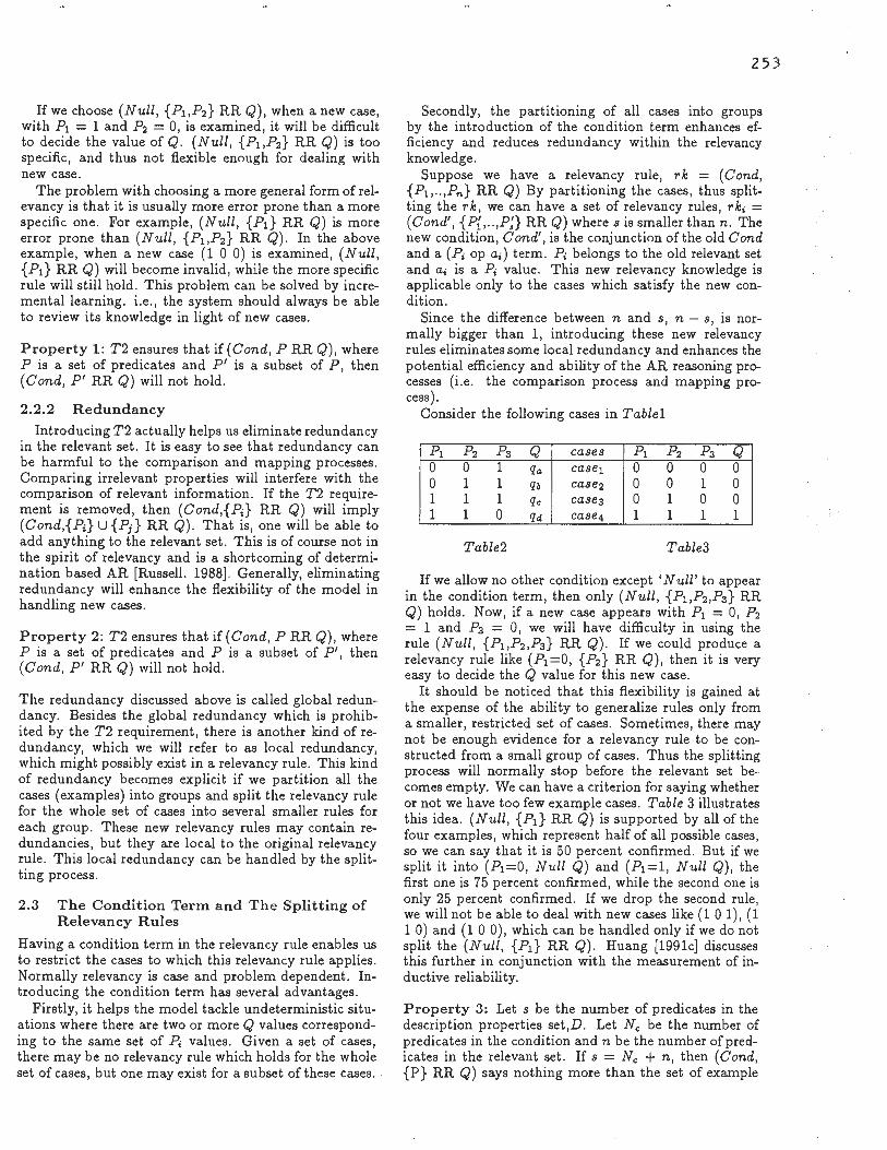
Ifwe choose (Null, {Pi,P2} RR Q), when a new case, with P1 = 1 and P2 = 0, is examined, it will be difficult to decide the value of Q. (Null, {Pi,P2} RR Q) is too specific, and thus not flexible enough for dealing with new case.

The problem with choosing a more general form of rel­evancy is that it is usually more error prone than a more specific one . For example, (Null, {Pi} RR Q) is more error prone than (Null, {Pi,P2} RR Q). In the above example, when a new case (1 0 0) is examined, (Null, {Pi} RR Q) will become invalid, while the more specific rule will still hold. This problem can be solved by incre­mental learning. i.e ., the system should always be able to review its knowledge in light of new cases.

Property 1 : T2 ensures that if (Cond, P RR Q), where P is a set of predicates and P' is a subset of P, then (Cond, P' RR Q) will not hold.

2.2.2 Redundancy

Introducing T2 actually helps us eliminate redundancy in the relevant set. It is easy to see that redundancy can be harmful to the comparison and mapping processes. Comparing irrelevant properties will interfere with the comparison of relevant information. If the T2 require­ment is removed, then (Cond,{Pi} RR Q) will imply (Cond,{Pi} U {Pj} RR Q). That is, one will be able to add anything to the relevant set . This is of course not in the spirit of relevancy and is a shortcoming of determi­nation based AR [Russell. 1988] . Generally, eliminating redundancy will enhance the flexibility of the model in handling new cases.

Property 2 : T2 ensures that if (Cond, P RR Q), where P is a set of predicates and P is a subset of P', then (Cond, P ' RR Q) will not hold.

The redundancy discussed above is called global redun­dancy. Besides the global redundancy which is prohib­ited by the T2 requirement, there is another kind of re­dundancy, which we will refer to as local redundancy, which might possibly exist in a relevancy rule . This kind of redundancy becomes explicit if we partition all the cases (examples) into groups and split the relevancy rule for the whole set of cases into several smaller rules for each group . These new relevancy rules may contain re­dundancies, but they are local to the original relevancy rule . This local redundancy can be handled by the split­ting process .

2.3 The Condition Term and The Splitting of Relevancy Rules

Having a condition term in the relevancy rule enables us to restrict the cases to which this relevancy rule applies. Normally relevancy is case and problem dependent . In­troducing the condition term has several advantages.

Firstly, it helps the model tackle undeterministic situ­ations where there are two or more Q values correspond­ing to the same set of Pi values. Given a set of cases, there may be no relevancy rule which holds for the whole set of cases, but one may exist for a subset of these cases.

2 53

Secondly, the partitioning of all cases into groups by the introduction of the condition term enhances ef­ficiency and reduces redundancy within the relevancy knowledge.

Suppose we have a relevancy rule , rk = (Cond , {Pi, .. ,Pn} RR Q) By partitioning the cases , thus split­ting the rk, we can have a set of relevancy rules, rki = (Cond', {P{, .. ,P;} RR Q) wheres is smaller than n . The new condition, Cond' , is the conjunction of the old Cond and a (Pi op ai) term. Pi belongs to the old relevant set and ai is a Pi value. This new relevancy knowledge is applicable only to the cases which satisfy the new con­dition .

Since the difference between n and s, n - s , is nor­mally bigger than 1, introducing these new relevancy rules eliminates some local redundancy and enhances the potential efficiency and ability of the AR reasoning pro­cesses (i .e. the comparison process and mapping pro­cess).

Consider the following cases in Table!

Pi P2 Pa Q cases Pi P2 Pa Q 0 0 1 qa case1 0 0 0 0 0 1 1 qb case2 0 0 1 0 1 1 1 qc casea 0 1 0 0 1 1 0 Qd case4 1 1 1 1

Table2 Table3

If we allow no other condition except 'Null' to appear in the condition term, then only (Null, {Pi,P2,Pa} RR Q) holds. Now, if a new case appears with Pi = 0, P2 = 1 and Pa = 0, we will have difficulty in using the rule (Null, {Pi,P2,Pa} RR Q) . If we could produce a relevancy rule like ( Pi = 0, { P2} RR Q), then it is very easy to decide the Q value for this new case.

It should be noticed that this flexibility is gained at the expense of the ability to generalize rules only from a smaller, restricted set of cases. Sometimes, there may not be enough evidence for a relevancy rule to be con­structed from a small group of cases. Thus the splitting process will normally stop before the relevant set be­comes empty. We can have a criterion for saying whether or not we have too few example cases . Table 3 illustrates this idea. (Null, {Pi} RR Q) is supported by all of the four examples, which represent half of all possible cases, so we can say that it is 50 percent confirmed. But if we split it into (Pi= O, Null Q) and (Pi = l, Null Q) , the first one is 75 percent confirmed, while the second one is only 25 percent confirmed. If we drop the second rule, we will not be able to deal with new cases like (1 0 1), (1 1 0) and (1 0 0), which can be handled only if we do not split the (Null, {Pi} RR Q) . Huang [1991c] discusses this further in conjunction with the measurement of in­ductive reliability.

Property 3: Let s be the number of predicates in the description properties set ,D . Let N e be the number of predicates in the condition and n be the number of pred­icates in the relevant set . Ifs = N e + n, then (Cond, {P} RR Q) says nothing more than the set of example

254

cases in an AR paradigm where similarity is defined by identity [Huang, 1991a] . That is, this rule will not help the system to deal with new cases.

In other words, splitting a bigger rule into small ones enables generalization. It is the generalization that in­troduces new knowledge into the system. For example, in table 2, (Null, {Pi,P2 ,P3 } RR Q) gives us nothing more than the four cases listed. But (Pi =O, {P2} RR Q) says more than the first two cases, and (Pi=O, {P3}

RR Q) says more than the last two cases.

3 Inductive Acquisition of Relevancy Rules

The relevancy rule based AR system is based upon the availability of relevancy knowledge, therefore, the acqui­sition of the relevancy rule becomes a critical problem. Conventionally, there are three ways of acquiring knowl­edge. The first one is to ask the user to supply the system with a set of relevancy rules. This is an efficient way if there are domain experts available. A good human computer interface and a method for eliciting relevancy knowledge can be a great help but is not within the scope of this paper. The second method is logical deduction. Once the logical properties of the knowledge are found and expressed in the form of implication rules, the de­duction of new rules from known ones becomes possible [Huang, 1991b] . The third way is the method of acquir­ing rules by induction. Given a set of experiences, an inductive system will produce a set of rules. These rules should satisfy certain criteria. In the following subsec­tions, only the inductive method will be addressed .

3.1 Inductive Learning

Traditionally, inductive learning refers to the process of generating descriptions or forming regularity rules from a set of data or facts. These generated descriptions or rules should account for the original data. Inductive meth­ods have a correlational nature. Basically, they examine some facts or examples and form concepts or rules by computing the commonality and difference among these examples.

The method described here is learning by searching and evaluating. Given a set of properties, D, and a tar­get Q, the problem is to find those P, which are subsets of D, and the proper corresponding conditions so that (Cond, P RR Q) hold. That is it satisfies the definition of the relevancy relationship. In the inductive learning paradigm, the decision as to whether a relevancy rule is satisfactory or not is based upon its empirical evaluation.

3.2 Searching Strategies

The search proceeds through a space of all the subsets of D. This space has a lattice structure. The biggest element of this structure is the description set, D . The descendants of a node {P.;} are the subsets resulting from taking one of the P.; out of this node. At each node, con­dition can be added to improve its evaluation. 2 Search-

2In fact, the condition part of the relevancy rule forms a more complicate structure.

ing is guided by the following strategies.

• Searching starts from the description node, D .

• Selection is based upon the evaluation of each node .. The evaluation reflects the requirements of an ac­ceptable relevancy rule.

• If a node satisfies the requirements, then there is no need to search its descendant .

• At each level of the lattice, only the best 3 node is selected, all others will be abandoned.

• Only the immediate descendants of the best node · are generated for further evaluation.

• The generation of condition term comes into play if the best node is not acceptable because of unsatis- · factory Tl or IR evaluations.

• Condition term of a node is generated by a splitting process. The condition will partition the whole case space thus restrict the case space to which this node applies.

• The condition is chosen so that the resulting rules -cover the maximum amount of cases .

3 .3 Empirical Measures

In real world, the logical requirements described in sec­tion 2 can hardly be met . Normally, P will not exactly decide Q. In order to generate a relevancy rule from a set of real world cases, three empirical measures are em­ployed in the evaluation of a candidate relevancy rule, which correspond to Tl, T2 and inductive reliability re­spectively.

For Tl, an entropy function is used to measure the homogeneity of Q value,

Tlcase,(rk) rcases(P, Q)

= L prob(group.; ) x entropy(group.;)

where entropy(groupi) = - Li prob( qi) x log(prob( qi)) and group.; is the ith group if we partition all exam­ple cases according to their values on the P . The prob(group.;) is the proportion of group.; against all ex­amples. This is exactly the same as the proportional method in Quinlan's work. [Quinlan, 1983]

IfTlcases(rk ) <€,we say that this rk satisfies the Tl requirement. The€ is a threshold value for Tlcases (rk) to be satisfactory.

The measure of T2 is defined by using the Tl measure. if rca.e(P, Q) ~ €

T2cases(rk)

otherwise T2 cas es ( rk) is undefined or meaningless. For a relevancy rule, rk, to satisfy the T2, we require

that T2caw(rk) < 0. The inductive reliability (IR) measure concerns the

proportion of the training examples to the overall space of cases. Generally, more evidence will lead to a stronger belief in the generated rule, thus a higher IR. But the

3 Heuristics, such as restricted maximum generalization, are used.

IR is also dependent on how big the potential case space is. 'Intuitively, given a fixed number of example cases, the bigger the potential case space, the smaller the IR measurement should be. In the system, we require that the IR measure for a relevancy rule must be greater than a certain threshold, which is termed as the E_Jevel.

The following formula 4 is for the IR measurement,

IRc,ues (rk) = Mc N Ng X 2s- . -n

IRcaHs(rk) = 0 Ng = 0

where Mc is the number of examples satisfying the condi­tion. The denominator is the potential number of all pre­dictable cases satisfying the condition. Ng is the number of groups, if example cases satisfying the condition are divided according to the relevant set Pi, .. ,P., . 5 Thesis the number of independent predicates in the Description set, and Ne is the number of predicates in the condition. s 2: Ne+ n.

3.4 Splitting The Relevancy Rule: Its Affects U pan The Measurements

Splitting relevancy rule has been discussed in section 2.3. If we have rk = (Cond, {Pi, P2, .. P.,} RR Q) Then

rki, = (Condi, , {Pi , P2 , .. , Pi-1, Pi+1, .. , P.,} RR Q)

are results of splitting rk by using Pi. Here the 'Condi .' is the conjunction of the old Condition 'Cond' and 'a 'Pi op Pi,' term, where Pi, is a value of Pi, j E [1, n] .

We will see that splitting an existing relevancy rule, because of its unsatisfactory Tl or IR measurements is an important method of generating new relevanc; rules with satisfactory measurements . In this subsection, properties will be presented concerning the relationship between the splitting of relevancy rules and its effects upon of the Tl and IR measurements.

From the definition of the Tl measurement, it can be shown [Huang , 1991c] that If we split rk into rki , .. rki then 1

_,

Property 4: Mini=l {Tl(rki,)} ::; Tl(rk)

rki, is a new relevancy rule for groupj, which consists of all cases in which Pi = Pi, .

This means that splitting the relevancy rule is a way of reducing the Tl measurement, or finding a new relevancy rule with a smaller Tl measurement.

From the definition of IR we can see that if a rele­vancy rule rk is broken into some more restricted ones rki, thus partitioning the example cases into groups, th~ following unequation hold

Property 5: IR(rk) ::; Max{IR(rki)}

This property says splitting a relevancy rule will at least

4This is a. simplified formula. . For deta.ils see (Hua.ng, 1991c)

5 Ng = 1 if n = 0 a.nd Mc =f. 0. Actually N9 = 0 implies Mc = 0, and vice versa.

255

increase the inductive reliabilities of some of the newly created relevancy rules.

Similarly, we can use Pk, which is not in the relevant set, to split a relevancy rule . The above two properties hold for this splitting as well .

3.5 Algorithm Outline

Given a set of example cases S, a description set D and a problem Q, this learning algorithm first sets the initial thresholds for € and E_level, then it puts the root rele­vancy rule, (Null, D RR Q) into the result set R . The R is a set of candidate relevancy rules. The evaluation of the rule, the splitting of the rule and the process of reducing redundancy then follow .

The evaluation process decides whether a relevancy rule, rk, is acceptable or not . For every rule in R, it computes the three empirical measures, to see if

(i) Tls(rk)::; e (ii) T2s(rk ) ::; 0 (iii) IRs(rk) 2: E-1evel

If (i), (ii) and (iii) are all satisfied, this process keeps this rk in R. If either (iii) or (i) are not true, it performs a splitting process for this rk. If (i), (iii) are true, but not(ii), it attempts to reduce redundancy for this rk .

The splitting process takes a relevancy rule , rk = (Cond, P RR Q), split it into rki = (Cond and P1, = Pk,, P -{Pk} RR Q) . P1, is chosen according to the general acceptance of all the rki, which is a function of the num­ber of example cases and the potential new cases these acceptable rki cover.

Reducing redundancy for ark = (Cond, P RR Q) is simply a question of removing the Pk, where P1, is the predicate corresponding to the maximum operation in the T2 measurement formula. If there are more than one of such Pi the one with the least variation in its values will be chosen. It will enable us to achieve the relevancy rule with the maximum generality.

3.6 Example

Based upon the strategies and evaluation measures, an experimental system of inductive learning of relevancy rules has been developed. Experiments has been carried out in the domains of a small block world, an animal tax­onomy problem, and a national flag description problem. These results have shown that relevancy rules in most cases have a very clear and understandable meaning. Us­ing these relevancy rules, the AR engine can solve new problems . More experiences have resulted in stronger relevancy rules, which will enable the AR engine to han­dle more new problems correctly. [Huang, 1991a;1991c]

In this section, this method is illustrated in a simple Block Moving Problem. Our problem in this block world will be briefly introduced. Then the relevancy knowledge learned from the experience is given. We will also see that using this knowledge, the problem can be solved correctly in certain cases.

This block world contains a three dimensional space, a block and a robot arm. Each dimension of the space has only two possible positions. The block may take one of two different shapes and may have one of two different

256

colours. The job of the robot arm is to move the block from an initial position to a target position.

There are two tools the robot arm may use, each cor­responding to a shape of the block. The robot arm may move one position in one of six direct ions if possible. There are no explicit rules about which tool should be used or which action should be taken for a given problem case.

Our model is to learn the relevancy rules from the experiences supplied. These relevancy rules will enable the AR engine to guide the robot to solve a new problem analogically.

Table 4 describes one set of experiences

Initial goal Motor Position I I Position I I Directions

X y z C s X y z T u L F P1 P2 P3 P4 Ps Ps P1 Pa Q1 Q2 Q3 Q4 0 0 0 0 0 0 1 1 1 n r n 0 0 1 0 0 0 1 1 1 n n f 0 0 0 0 0 0 1 0 1 n n f 0 0 0 0 1 0 1 1 0 n r n 0 0 1 0 1 0 1 1 0 n n f 0 1 0 0 0 0 0 0 1 n n b 0 1 0 0 0 0 1 1 1 n r n 0 0 1 1 0 0 1 1 1 n n f

Table 4 Training Experiences

where C = Colour; S = Shape; T = Tool; X (up-down) , Y (forward-backward), Z (right-left) are coordinates; U = Up-Down Motor; L = Left-Right Motor; F = Forward­Backward Motor; r = right; 1 = left; f =forward; b = backward; u = up; d = down; n = null.

Applying the induction process, the following relevan­cies have been produced among others, with € = 0.1, and E..level = 1/6. This EJ.evel is quite small. This is because the examples we supply to the model represent a very small portion of all the possible cases.

rk1, (P1 = 0 and Ps = 0 and P2 = 0, {Ps} RR Q1) rk1a, (Pi = 0 and Ps = 0 and Pa = 1, {Ps} RR Q1) rk2 , (Pi = 0 and P4 = 0 and Ps = 0 , Null RR Q2 ) rk2a, (Pi= 0 and Ps = 0 and P1 = 1, Null RR Q2 ) rk3, (Pi = 0 and Ps = 0, {P3,Pa} RR Q3) rk4, (Pi = 0 and Ps = 0, {P2,P3 1Pa} RR Q4 ) These relevancy rules give some useful regularities

within certain case sub-spaces. Rules rk1 and rk1a say that to decide which tool to use, only the shape of the block is relevant. Rules rk2 and rk2a say that Q2 is a constant. This is because we do not have any experience of moving the block up and down. To decide the action of the left-right motor, rk3 says that we only need to con­sider the Z coordinates of the initial and target cases. Rule rk4 says that in order to make a forward-backward move, we need to consider not only the Y coordinate of the initial situation, but also the Z coordinates of the initial and the goal situations. This can be explained by the fact that the right-left motor has priority over the forward- backward motor.

Now let us use these relevancy rules for the testing cases in the Test Cases Table. Relevancy rule guided

AR can be carried out in two directions: data directed or goal directed. The latter variant is described here.

Given a goal in a target case, the relevancy rule based AR process is as follow. ·

(i) Find a relevancy rule with the goal as its Q part . and where the target case satisfies the condition part o: the rule.

(ii) Find an experience case, which satisfies the 'con­dition', and shares the same values of properties in th€ relevant set of the relevancy rule with the target case .

(iii) Introduce the value of the goal in the experience case into the target. In complex situation, transforma­tion is necessary. Building a tower analogically in a mul­tiple blocks world is an example [Huang , 1991a]. I

(iv) Verify this value in the target case.

test ImLPos C s a 0 0 0 0 1 n n b 0 0 0 1 0 n n C 0 0 0 1 1 n n d 0 0 0 1 1 n r n e 0 0 0 1 0 n r n f 0 0 1 1 1 n n f g 0 1 0 0 0 n n n h 0 0 1 1 1 n ? f j 0 0 1 0 0 n ? f k 0 1 0 0 1 ? n b

Table 5 Test Cases Results

The results of applying this process and using the above relevancy knowledge are shown by table 5. Tests a to g have reached the correct conclusions. In Tests h and j, the model failed to generate actions for the Left-Right motor because of its lack of experience of moving left. In Test k it failed to generate the Up-Down motor ac­tion. The reason is that the model has not experienced enough cases in which the P1 property takes O value and therefore has not generated a relevancy rule for Q2 which applies to new cases with P7 = 0.

4 Conclusion

Knowledge guided AR is a way of making AR justifi- · able. The knowledge used in AR is different from that of conventional deductive reasoning mechanisms. This pa­per proposes the relevancy rule as a form of knowledge which can support the AR process. Relevancy knowl­edge describes a kind of general relationship between the properties of a given world. This is in contrast with Greiner's abstract formula , which describes a strong the­orem in an abstract domain applied to several different concrete domains. Automated acquisition of relevancy rules is easier than that of abstract formulae . Therefore the relevancy rule based AR model has a better chance of increasing its power. The relevancy rule considers the relevancy of a property for deciding another prop­erty is important . This is an enhancement of Russell's determination rule, which considers only determination information. Because considering irrelevant information may interfere with the analogical comparison. Relevancy rules enable an AR system to deal with new cases bet-

ter than a determination rule does. However, no attempt has been made to empirically or experimentally compare the results of relevancy rule based AR with that of any other methods, as that is beyond the scope of this paper.

Moreover, no comparison has been made between AR and conventional deductive methods. This is a field which lacks substantial work. So far, most authors con­sider AR to be a compliment to deductive methods. Only when the latter fails to produce results then AR comes into play. [Holland et al., 1989] There is no justi­fiable reason for giving deductive methods priority over AR in solving problems. Research on the relevancy rule may shed light on the study of the relationship between AR and deductive methods. One clue is that the conven­tional form of production rule has only a trivial differ­ence to a relevancy rule with a 'Null' as it relevant set. Can we say that deductive reasoning is a special form of AR? Study of the evolution of relevancy knowledge may provide a hint for explaining why both schemes of reasoning exist and how they relate to each other. This explanation seems more profound than simply claiming AR and deductive methods are completely different and compliment each other.

Learning is an important field of study in AI. An intel­ligent system need to be able to learn , i.e. be capable of improving its ability automatically. The relevancy rule based AR system is no exception since successful rea­soning in this system is based upon the availability of relevancy knowledge.

An important source of knowledge is experience . In­ductive learning of relevancy rules is a method of ac­quiring relevancy laws from cases from experience. This paper has proposed a way of searching and evaluating candidate relevancy rules . The nature of this method is to select a promising candidate rule and check if it accounts for its experiences according to certain criteria.

In addition, This paper has defined three empirical measures for the relevancy rule . They are the sufficiency measure, the necessity measure and the inductive relia­bility measure . They first two correspond to the logical requirements of a relevancy rule. The third concerns the amount of evidence or experiences that support the candidate rule. The criteria are set, based upon these measures, for accepting a candidate relevancy rule.

The learning of relevancy rules is a new topic, conven­tional techniques, such as heuristics of non-exhaustive searching and the entropy measurement method, are used in the experimental inductive system. However, some unanswered questions remain. How should the thresholds for accepting a relevancy rule be decided in the first place? How should they be adjusted accord­ing to the performance of the system in dealing with new cases? At present, initial thresholds are set ac­cording to the proportion of exceptional cases to the whole case (for the c) and according to a prediction rate (for the E_level). For instance, if we allow one ex­ception in every ten cases on average, the c would be 0.9log(0.9)+0.llog(0.1). Adjustment of the thresholds can be based upon the error rate of the analogical argu­ments. New thresholds should result in the evolution of relevancy rules. Substantial work is needed in this area.

257

To conclude, this paper has shown that relevancy knowledge is a form of knowledge which supports jus­tifiable AR. The inductive learning method described here provides a way of automatic acquisition of relevancy knowledge. This increases the ability of the relevancy rule guided AR system. The work described in this pa­per provides a preliminary basis for further study.

Acknowledgements

The first author wishes to thank all parties of the Sino­British Friendship Scholarship Scheme for sponsoring his studies resulting this paper. He would also like to thank Gerard V. Conroy for helpful discussions.

References

[Greiner, 1988a] Russell Greiner. Abstraction-Based Analogical Inference. In David H. Helman (Ed.) Ana­logical Reasoning, Kluwer Academic Publisher, 1988.

[Greiner, 1988b] Russell Greiner. Learning by Under-standing Analogies . In Armand Priedits(Ed.), Ana­logica, Pitman Publishing, London, 1988.

[Holland, et al. , 1989] John H. Holland, Keith J . Holyoak, Richard E. Nisbett and Paul R . Thagard. Induction : Processes of Inference, Learning, and Dis­covery. MIT, London, 1989.

[Huang, 1991a] Ye Huang. Analogical Reasoning: The Use of Relevancy Rule. Internal Report, Computation Department, UMIST, UK, 1991.

[Huang, 1991b] Ye Huang. On Derivation of Relevancy Knowledge. Internal Report, Computation Depart­ment, UMIST, UK, 1991.

[Huang, 1991c] Ye Huang . On Inductive Acquisition of Relevancy Knowledge. Internal Report, Computation Department, UMIST, UK, 1991.

[Kedar-Cabelli, 1988a] Smadar Kedar-Cabelli . Analogy - From a Unified Perspective. In David H. Helman (Ed.), Analogical Reasoning, Kluwer Academic Pub­lisher, 1988.

[Kedar-Cabelli, 1988b] Smadar Kedar-Cabelli . Toward a Computational Model of Purpose-Directed Analogy. In Armand Priedits (Ed.), Analogica, Pitman Publish­ing, London, 1988.

[Quinlan, 1983] Ross Quinlan. Learning Efficient Clas­sification Procedures. In R.S. Michalski, J .G. Car­bone! and T .M. Mitchel (Eds.), Machine Learning: An Artificial Intelligence Approach, Ch. 15, Vol I, Tioga Press, Palo Alto, CA, 1983.

[Russell, 1988] Stuart J, Russell. The Use of Knowledge in Analogy and Induction. Pitman Publishing, Lon­don, 1988 .

[Vosniadou and Ortony, 1989] Stella Vosniadou and An­drew Ortony. Similarity and Analogy. Cambridge Press, 1989.