Maxwell’s Equations - University of Delawareweile/ELEG648Spring06/Resources/Maxwell... · Using...
73
Introduction Basic Theory The Frequency Domain Maxwell’s Equations Daniel S. Weile Department of Electrical and Computer Engineering University of Delaware ELEG 648—Maxwell’s Equations D. S. Weile Maxwell’s Equations
Transcript of Maxwell’s Equations - University of Delawareweile/ELEG648Spring06/Resources/Maxwell... · Using...

IntroductionBasic Theory
The Frequency Domain
Maxwell’s Equations
Daniel S. Weile
Department of Electrical and Computer EngineeringUniversity of Delaware
ELEG 648—Maxwell’s Equations
D. S. Weile Maxwell’s Equations
IntroductionBasic Theory
The Frequency Domain
Outline
1 Maxwell Equations, Units, and VectorsUnits and ConventionsMaxwell’s EquationsVector TheoremsConstitutive Relationships
2 Basic TheoryGeneralized CurrentDerivation of Poynting’s Theorem
3 The Frequency DomainPhasors and Maxwell’s EquationsComplex PowerBoundary Conditions
D. S. Weile Maxwell’s Equations

IntroductionBasic Theory
The Frequency Domain
Units and ConventionsMaxwell’s EquationsVector TheoremsConstitutive Relationships
Outline
1 Maxwell Equations, Units, and VectorsUnits and ConventionsMaxwell’s EquationsVector TheoremsConstitutive Relationships
2 Basic TheoryGeneralized CurrentDerivation of Poynting’s Theorem
3 The Frequency DomainPhasors and Maxwell’s EquationsComplex PowerBoundary Conditions
D. S. Weile Maxwell’s Equations
IntroductionBasic Theory
The Frequency Domain
Units and ConventionsMaxwell’s EquationsVector TheoremsConstitutive Relationships
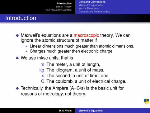
Introduction
Maxwell’s equations are a macroscopic theory. We canignore the atomic structure of matter if
Linear dimensions much greater than atomic dimensions.Charges much greater then electronic charge.
We use mksc units, that ism The meter, a unit of length,kg The kilogram, a unit of mass,
s The second, a unit of time, andC The coulomb, a unit of electrical charge.
Technically, the Ampère (A=C/s) is the basic unit forreasons of metrology, not theory.
D. S. Weile Maxwell’s Equations
IntroductionBasic Theory
The Frequency Domain
Units and ConventionsMaxwell’s EquationsVector TheoremsConstitutive Relationships
Variables
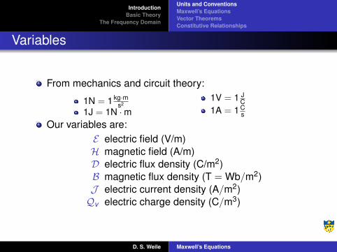
From mechanics and circuit theory:
1N = 1 kg·ms2
1J = 1N ·m1V = 1 J
C1A = 1 C
s
Our variables are:E electric field (V/m)H magnetic field (A/m)D electric flux density (C/m2)B magnetic flux density (T = Wb/m2)J electric current density (A/m2)Qv electric charge density (C/m3)
D. S. Weile Maxwell’s Equations

IntroductionBasic Theory
The Frequency Domain
Units and ConventionsMaxwell’s EquationsVector TheoremsConstitutive Relationships
Conventions
The normal to an open surfacebounded by a contour is relatedto the contour by the right handrule.
The normal to a closed surfacepoints out from the surface.
D. S. Weile Maxwell’s Equations
IntroductionBasic Theory
The Frequency Domain
Units and ConventionsMaxwell’s EquationsVector TheoremsConstitutive Relationships
Outline
1 Maxwell Equations, Units, and VectorsUnits and ConventionsMaxwell’s EquationsVector TheoremsConstitutive Relationships
2 Basic TheoryGeneralized CurrentDerivation of Poynting’s Theorem
3 The Frequency DomainPhasors and Maxwell’s EquationsComplex PowerBoundary Conditions
D. S. Weile Maxwell’s Equations
IntroductionBasic Theory
The Frequency Domain
Units and ConventionsMaxwell’s EquationsVector TheoremsConstitutive Relationships
Maxwell’s Equations in Integral Form
©∫∫D · dS =
∫∫∫Qv dv
©∫∫B · dS = 0∮
E · dl = − ddt
∫∫B · dS∮
H · dl =∫∫J · dS +
ddt
∫∫D · dS
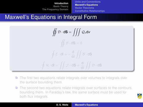
The first two equations relate integrals over volumes to integrals overthe surface bounding them.
The second two equations relate integrals over surfaces to the contoursbounding them. In Faraday’s law, the same surface must be used forboth flux integrals.
D. S. Weile Maxwell’s Equations

IntroductionBasic Theory
The Frequency Domain
Units and ConventionsMaxwell’s EquationsVector TheoremsConstitutive Relationships
Maxwell’s Equations in Integral Form
©∫∫D · dS =
∫∫∫Qv dv
©∫∫B · dS = 0∮
E · dl = − ddt
∫∫B · dS∮
H · dl =∫∫J · dS +
ddt
∫∫D · dS
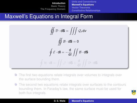
The first two equations relate integrals over volumes to integrals overthe surface bounding them.
The second two equations relate integrals over surfaces to the contoursbounding them. In Faraday’s law, the same surface must be used forboth flux integrals.
D. S. Weile Maxwell’s Equations
IntroductionBasic Theory
The Frequency Domain
Units and ConventionsMaxwell’s EquationsVector TheoremsConstitutive Relationships
Maxwell’s Equations in Integral Form
©∫∫D · dS =
∫∫∫Qv dv
©∫∫B · dS = 0∮
E · dl = − ddt
∫∫B · dS∮
H · dl =∫∫J · dS +
ddt
∫∫D · dS
The first two equations relate integrals over volumes to integrals overthe surface bounding them.
The second two equations relate integrals over surfaces to the contoursbounding them. In Faraday’s law, the same surface must be used forboth flux integrals.
D. S. Weile Maxwell’s Equations

IntroductionBasic Theory
The Frequency Domain
Units and ConventionsMaxwell’s EquationsVector TheoremsConstitutive Relationships
Conservation of Charge
C1
C2
S1S2
Consider a closed surface cleaved in half by an open surface.Using the Maxwell-Ampère Law in both directions gives∮
C1
H · dl =
∫∫S1
J · dS +ddt
∫∫S1
D · dS∮C2
H · dl =
∫∫S2
J · dS +ddt
∫∫S2
D · dS
D. S. Weile Maxwell’s Equations
IntroductionBasic Theory
The Frequency Domain
Units and ConventionsMaxwell’s EquationsVector TheoremsConstitutive Relationships
Conservation of Charge
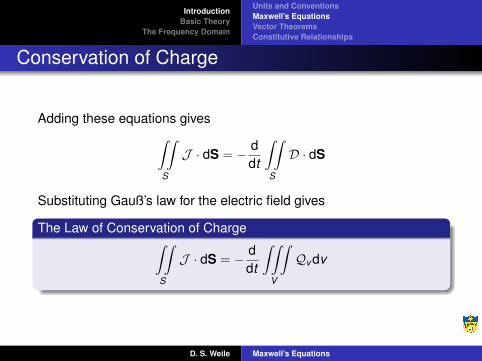
Adding these equations gives∫∫S
J · dS = − ddt
∫∫S
D · dS
Substituting Gauß’s law for the electric field gives
The Law of Conservation of Charge∫∫S
J · dS = − ddt
∫∫∫V
Qv dv
D. S. Weile Maxwell’s Equations
IntroductionBasic Theory
The Frequency Domain
Units and ConventionsMaxwell’s EquationsVector TheoremsConstitutive Relationships
Outline
1 Maxwell Equations, Units, and VectorsUnits and ConventionsMaxwell’s EquationsVector TheoremsConstitutive Relationships
2 Basic TheoryGeneralized CurrentDerivation of Poynting’s Theorem
3 The Frequency DomainPhasors and Maxwell’s EquationsComplex PowerBoundary Conditions
D. S. Weile Maxwell’s Equations
IntroductionBasic Theory
The Frequency Domain
Units and ConventionsMaxwell’s EquationsVector TheoremsConstitutive Relationships
The Divergence Theorem
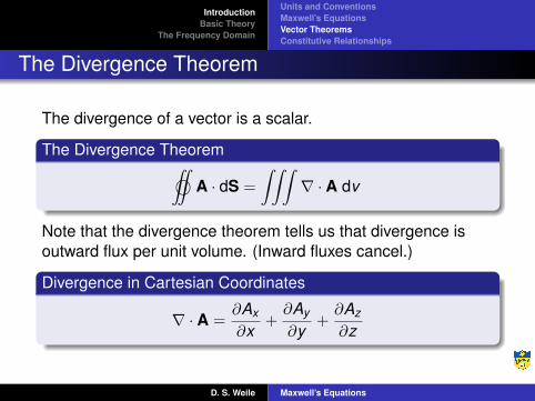
The divergence of a vector is a scalar.
The Divergence Theorem
©∫∫
A · dS =
∫∫∫∇ · A dv
Note that the divergence theorem tells us that divergence isoutward flux per unit volume. (Inward fluxes cancel.)
Divergence in Cartesian Coordinates
∇ · A =∂Ax
∂x+∂Ay
∂y+∂Az
∂z
D. S. Weile Maxwell’s Equations
IntroductionBasic Theory
The Frequency Domain
Units and ConventionsMaxwell’s EquationsVector TheoremsConstitutive Relationships
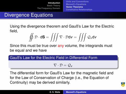
Divergence Equations
Using the divergence theorem and Gauß’s Law for the Electricfield,
©∫∫D · dS =
∫∫∫∇ · Ddv =
∫∫∫Qv dv
Since this must be true over any volume, the integrands mustbe equal and we have
Gauß’s Law for the Electric Field in Differential Form
∇ · D = Qv
The differential form for Gauß’s Law for the magnetic field andfor the Law of Conservation of Charge (i.e., the Equation ofContinuity) may be derived similarly.
D. S. Weile Maxwell’s Equations

IntroductionBasic Theory
The Frequency Domain
Units and ConventionsMaxwell’s EquationsVector TheoremsConstitutive Relationships
Stokes’s Theorem
The curl of a vector is a vector.
Stokes’s Theorem ∮A · dl =
∫∫∇× A · dS
Note that the curl is the rotation per unit area, with directiongiven by the right-hand rule. (Internal circulation cancels.)
Curl in Cartesian Coordinates
∇× A =
(∂Az
∂y−∂Ay
∂z
)ax +
(∂Ax
∂z− ∂Az
∂x
)ay +
(∂Ay
∂x− ∂Ax
∂y
)az
D. S. Weile Maxwell’s Equations
IntroductionBasic Theory
The Frequency Domain
Units and ConventionsMaxwell’s EquationsVector TheoremsConstitutive Relationships
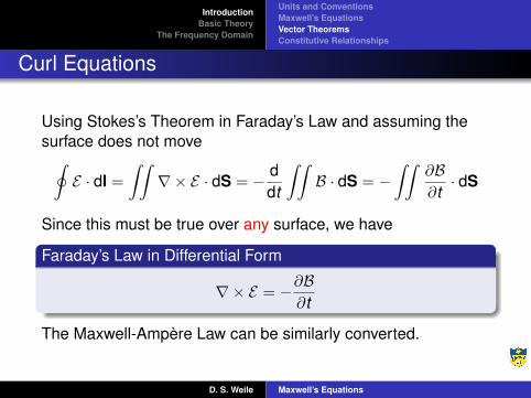
Curl Equations
Using Stokes’s Theorem in Faraday’s Law and assuming thesurface does not move∮E · dl =
∫∫∇× E · dS = − d
dt
∫∫B · dS = −
∫∫∂B∂t· dS
Since this must be true over any surface, we have
Faraday’s Law in Differential Form
∇× E = −∂B∂t
The Maxwell-Ampère Law can be similarly converted.
D. S. Weile Maxwell’s Equations

IntroductionBasic Theory
The Frequency Domain
Units and ConventionsMaxwell’s EquationsVector TheoremsConstitutive Relationships
Maxwell’s Equations in Differential Form
Maxwell’s Equations
∇ · D = Qv
∇ · B = 0
∇× E = −∂B∂t
∇×H = J +∂D∂t
Continuity Equation
∇ · J = −∂Qv
∂t
D. S. Weile Maxwell’s Equations
IntroductionBasic Theory
The Frequency Domain
Units and ConventionsMaxwell’s EquationsVector TheoremsConstitutive Relationships
Outline
1 Maxwell Equations, Units, and VectorsUnits and ConventionsMaxwell’s EquationsVector TheoremsConstitutive Relationships
2 Basic TheoryGeneralized CurrentDerivation of Poynting’s Theorem
3 The Frequency DomainPhasors and Maxwell’s EquationsComplex PowerBoundary Conditions
D. S. Weile Maxwell’s Equations
IntroductionBasic Theory
The Frequency Domain
Units and ConventionsMaxwell’s EquationsVector TheoremsConstitutive Relationships
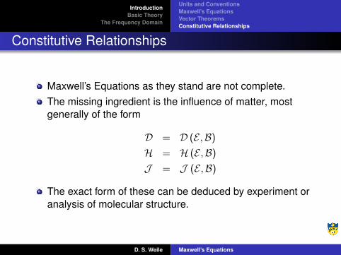
Constitutive Relationships
Maxwell’s Equations as they stand are not complete.The missing ingredient is the influence of matter, mostgenerally of the form
D = D (E ,B)H = H (E ,B)J = J (E ,B)
The exact form of these can be deduced by experiment oranalysis of molecular structure.
D. S. Weile Maxwell’s Equations

IntroductionBasic Theory
The Frequency Domain
Units and ConventionsMaxwell’s EquationsVector TheoremsConstitutive Relationships
Free Space
In vacuum (or, for all practical purposes, air) the constitutiverelationships are
D = ε0EB = µ0HJ = 0
We will see later that c, the speed of light in vacuum, is givenby the formula
The Speed of Light
c =1
√ε0µ0
= 2.99792458× 10⁸m/s
D. S. Weile Maxwell’s Equations

IntroductionBasic Theory
The Frequency Domain
Units and ConventionsMaxwell’s EquationsVector TheoremsConstitutive Relationships
Free Space
The value of the speed of light is set by internationalagreement, and serves to define the meter. (The second isdefined by another standard.)A useful approximation is c = 3× 10⁸m/sThe internationally agreed upon value for the permeabilityof free space is
µ0 = 4π × 10−7H/m
(By definition, 1H=1V-s/A.)The above implies
ε0 ≈ 8.854× 10⁻¹²F/m ≈ 10−9
36πF/m
(By definition, 1F = 1 C/V)
D. S. Weile Maxwell’s Equations
IntroductionBasic Theory
The Frequency Domain
Units and ConventionsMaxwell’s EquationsVector TheoremsConstitutive Relationships
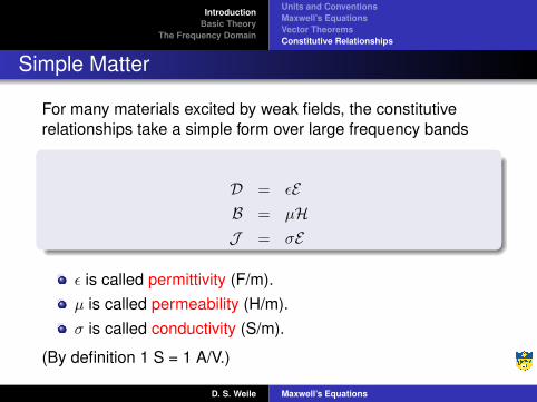
Simple Matter
For many materials excited by weak fields, the constitutiverelationships take a simple form over large frequency bands
D = εEB = µHJ = σE
ε is called permittivity (F/m).µ is called permeability (H/m).σ is called conductivity (S/m).
(By definition 1 S = 1 A/V.)
D. S. Weile Maxwell’s Equations
IntroductionBasic Theory
The Frequency Domain
Units and ConventionsMaxwell’s EquationsVector TheoremsConstitutive Relationships
Simple Matter Terminology
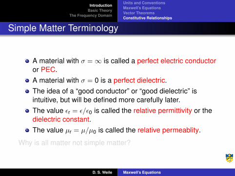
A material with σ =∞ is called a perfect electric conductoror PEC.A material with σ = 0 is a perfect dielectric.The idea of a “good conductor” or “good dielectric” isintuitive, but will be defined more carefully later.The value εr = ε/ε0 is called the relative permittivity or thedielectric constant.The value µr = µ/µ0 is called the relative permeablity.
Why is all matter not simple matter?
D. S. Weile Maxwell’s Equations

IntroductionBasic Theory
The Frequency Domain
Units and ConventionsMaxwell’s EquationsVector TheoremsConstitutive Relationships
Simple Matter Terminology
A material with σ =∞ is called a perfect electric conductoror PEC.A material with σ = 0 is a perfect dielectric.The idea of a “good conductor” or “good dielectric” isintuitive, but will be defined more carefully later.The value εr = ε/ε0 is called the relative permittivity or thedielectric constant.The value µr = µ/µ0 is called the relative permeablity.
Why is all matter not simple matter?
D. S. Weile Maxwell’s Equations

IntroductionBasic Theory
The Frequency Domain
Units and ConventionsMaxwell’s EquationsVector TheoremsConstitutive Relationships
Complicated Matter
In general linear matter, the constitutive parameter is acausal function of time to be convolved with theappropriate variable, i.e.
D(t) =∫ t
−∞ε(t − τ)E(τ)dτ
In nonlinear matter, the constitutive parameters arefunctions of the field variables, i.e.
ε = ε(E).
In short, in such media, the fields cannot be computed byconvolution in time.
D. S. Weile Maxwell’s Equations

IntroductionBasic Theory
The Frequency Domain
Units and ConventionsMaxwell’s EquationsVector TheoremsConstitutive Relationships
Complicated Matter
In anisotropic matter, the constitutive parameter is a matrixso that, for instance, E and D are not parallel. Normalmatter is called isotropic.Finally, in chiral matter, D is a function (generally linear) ofboth E and B, with a similar relation for H.In this class, we will never deal with anything morecomplicated then general linear matter.
D. S. Weile Maxwell’s Equations
IntroductionBasic Theory
The Frequency Domain
Generalized CurrentDerivation of Poynting’s Theorem
Outline
1 Maxwell Equations, Units, and VectorsUnits and ConventionsMaxwell’s EquationsVector TheoremsConstitutive Relationships
2 Basic TheoryGeneralized CurrentDerivation of Poynting’s Theorem
3 The Frequency DomainPhasors and Maxwell’s EquationsComplex PowerBoundary Conditions
D. S. Weile Maxwell’s Equations

IntroductionBasic Theory
The Frequency Domain
Generalized CurrentDerivation of Poynting’s Theorem
Generalized Current
Ampère’s law was originally
∇×H = J .
Maxwell amended this to include the “displacementcurrent”
J d =∂D∂t
He did this to ensure conservation of charge, andenvisioned it as a real current flow in the ether. This view isincorrect, but the definition is useful.
D. S. Weile Maxwell’s Equations
IntroductionBasic Theory
The Frequency Domain
Generalized CurrentDerivation of Poynting’s Theorem
Generalized Current
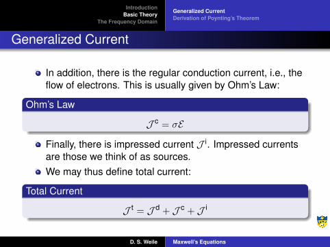
In addition, there is the regular conduction current, i.e., theflow of electrons. This is usually given by Ohm’s Law:
Ohm’s Law
J c = σE
Finally, there is impressed current J i. Impressed currentsare those we think of as sources.We may thus define total current:
Total Current
J t = J d + J c + J i
D. S. Weile Maxwell’s Equations

IntroductionBasic Theory
The Frequency Domain
Generalized CurrentDerivation of Poynting’s Theorem
Generalized Current
In a similar vein,
Md =∂B∂t
can be though of as a magnetic displacement current.“Voltage” sources can be envisioned as impressedmagnetic currentMi.Total magnetic current is then
Total Magnetic Current
Mt =Md +Mi
D. S. Weile Maxwell’s Equations

IntroductionBasic Theory
The Frequency Domain
Generalized CurrentDerivation of Poynting’s Theorem
Generalized Current
In terms of this generalized current, the curl equations become
∇× E = −Mt
∇×H = J t
A Vector Identity
∇ · ∇ × A = 0
A Theorem
∇ ·Mt = ∇ · J t = 0
D. S. Weile Maxwell’s Equations

IntroductionBasic Theory
The Frequency Domain
Generalized CurrentDerivation of Poynting’s Theorem
Generalized Current
In terms of this generalized current, the curl equations become
∇× E = −Mt
∇×H = J t
A Vector Identity
∇ · ∇ × A = 0
A Theorem
∇ ·Mt = ∇ · J t = 0
D. S. Weile Maxwell’s Equations

IntroductionBasic Theory
The Frequency Domain
Generalized CurrentDerivation of Poynting’s Theorem
Generalized Current
In terms of this generalized current, the curl equations become
∇× E = −Mt
∇×H = J t
A Vector Identity
∇ · ∇ × A = 0
A Theorem
∇ ·Mt = ∇ · J t = 0
D. S. Weile Maxwell’s Equations
IntroductionBasic Theory
The Frequency Domain
Generalized CurrentDerivation of Poynting’s Theorem
Proof of a Vector Identity
C1
C2
S1S2
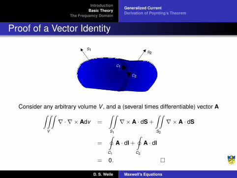
Consider any arbitrary volume V , and a (several times differentiable) vector A∫∫∫V
∇ · ∇ × Adv =
∫∫S1
∇× A · dS +
∫∫S2
∇× A · dS
=
∮C1
A · dl +∮C2
A · dl
= 0. �
D. S. Weile Maxwell’s Equations

IntroductionBasic Theory
The Frequency Domain
Generalized CurrentDerivation of Poynting’s Theorem
Generalized Current
We thus see that total current is solenoidal; that is it has nosources and sinks. Here is a circuit that demonstrates all threetypes:
Impressed
Current
Conduction Current
Displacement
Current
D. S. Weile Maxwell’s Equations
IntroductionBasic Theory
The Frequency Domain
Generalized CurrentDerivation of Poynting’s Theorem
Outline
1 Maxwell Equations, Units, and VectorsUnits and ConventionsMaxwell’s EquationsVector TheoremsConstitutive Relationships
2 Basic TheoryGeneralized CurrentDerivation of Poynting’s Theorem
3 The Frequency DomainPhasors and Maxwell’s EquationsComplex PowerBoundary Conditions
D. S. Weile Maxwell’s Equations
IntroductionBasic Theory
The Frequency Domain
Generalized CurrentDerivation of Poynting’s Theorem
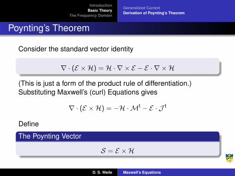
Poynting’s Theorem
Consider the standard vector identity
∇ · (E ×H) = H · ∇ × E − E · ∇ ×H
(This is just a form of the product rule of differentiation.)Substituting Maxwell’s (curl) Equations gives
∇ · (E ×H) = −H ·Mt − E · J t
Define
The Poynting Vector
S = E ×H
D. S. Weile Maxwell’s Equations
IntroductionBasic Theory
The Frequency Domain
Generalized CurrentDerivation of Poynting’s Theorem
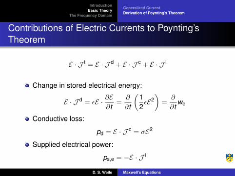
Contributions of Electric Currents to Poynting’sTheorem
E · J t = E · J d + E · J c + E · J i
Change in stored electrical energy:
E · J d = εE · ∂E∂t
=∂
∂t
(12εE2)
=∂
∂twe
Conductive loss:
pd = E · J c = σE2
Supplied electrical power:
ps,e = −E · J i
D. S. Weile Maxwell’s Equations
IntroductionBasic Theory
The Frequency Domain
Generalized CurrentDerivation of Poynting’s Theorem
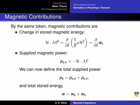
Magnetic Contributions
By the same token, magnetic contributions areChange in stored magnetic energy:
H ·Md =∂
∂t
(12µH2
)=
∂
∂twh
Supplied magnetic power:
ps,h = −H ·Mi
We can now define the total supplied power
ps = ps,e + ps,h,
and total stored energy,
w = we + wh.
D. S. Weile Maxwell’s Equations
IntroductionBasic Theory
The Frequency Domain
Generalized CurrentDerivation of Poynting’s Theorem
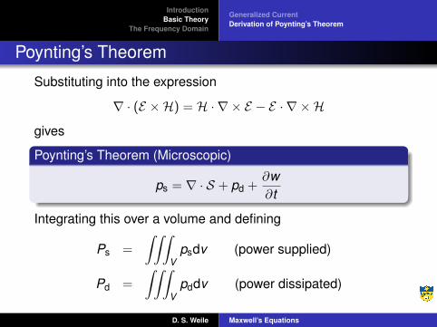
Poynting’s Theorem
Substituting into the expression
∇ · (E ×H) = H · ∇ × E − E · ∇ ×H
gives
Poynting’s Theorem (Microscopic)
ps = ∇ · S + pd +∂w∂t
Integrating this over a volume and defining
Ps =
∫∫∫V
psdv (power supplied)
Pd =
∫∫∫V
pddv (power dissipated)
D. S. Weile Maxwell’s Equations

IntroductionBasic Theory
The Frequency Domain
Generalized CurrentDerivation of Poynting’s Theorem
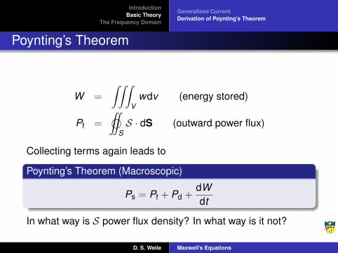
Poynting’s Theorem
W =
∫∫∫V
wdv (energy stored)
Pf = ©∫∫
SS · dS (outward power flux)
Collecting terms again leads to
Poynting’s Theorem (Macroscopic)
Ps = Pf + Pd +dWdt
In what way is S power flux density? In what way is it not?
D. S. Weile Maxwell’s Equations
IntroductionBasic Theory
The Frequency Domain
Generalized CurrentDerivation of Poynting’s Theorem
Poynting’s Theorem
W =
∫∫∫V
wdv (energy stored)
Pf = ©∫∫
SS · dS (outward power flux)
Collecting terms again leads to
Poynting’s Theorem (Macroscopic)
Ps = Pf + Pd +dWdt
In what way is S power flux density? In what way is it not?
D. S. Weile Maxwell’s Equations

IntroductionBasic Theory
The Frequency Domain
Phasors and Maxwell’s EquationsComplex PowerBoundary Conditions
Outline
1 Maxwell Equations, Units, and VectorsUnits and ConventionsMaxwell’s EquationsVector TheoremsConstitutive Relationships
2 Basic TheoryGeneralized CurrentDerivation of Poynting’s Theorem
3 The Frequency DomainPhasors and Maxwell’s EquationsComplex PowerBoundary Conditions
D. S. Weile Maxwell’s Equations
IntroductionBasic Theory
The Frequency Domain
Phasors and Maxwell’s EquationsComplex PowerBoundary Conditions
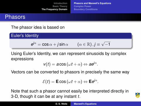
Phasors
The phasor idea is based on
Euler’s Identity
ejα = cosα+ j sinα (α ∈ R) , j ≡√−1
Using Euler’s Identity, we can represent sinusoids by complexexpressions
v(t) = a cos (ωt + α)⇔ aejα.
Vectors can be converted to phasors in precisely the same way
E(t) = E cos (ωt + α)⇔ Eejα.
Note that such a phasor cannot easily be interpreted directly in3-D, though it can be at any instant t .
D. S. Weile Maxwell’s Equations
IntroductionBasic Theory
The Frequency Domain
Phasors and Maxwell’s EquationsComplex PowerBoundary Conditions
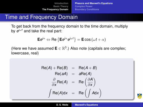
Time and Frequency DomainTo get back from the frequency domain to the time domain, multiplyby ejωt and take the real part:
Eejα ⇔ Re{
Eejαejωt} = E cos (ωt + α)
(Here we have assumed E ∈ R3.) Also note (capitals are complex;lowercase, real)
Re(A) + Re(B) = Re(A + B)
Re(aA) = aRe(A)∂
∂xRe(A) = Re
(∂A∂x
)∫
Re(A)dx = Re(∫
Adx)
D. S. Weile Maxwell’s Equations

IntroductionBasic Theory
The Frequency Domain
Phasors and Maxwell’s EquationsComplex PowerBoundary Conditions
A Justification
TheoremSuppose A,B ∈ C. Then
Re(Aejωt) = Re(Bejωt) ∀t ⇒ A = B
Proof.Inserting ωt = 0 into the assumption reveals that
Re(A) = Re(B).
Similarly, inserting ωt = π2 gives
Im(A) = Im(B).
D. S. Weile Maxwell’s Equations

IntroductionBasic Theory
The Frequency Domain
Phasors and Maxwell’s EquationsComplex PowerBoundary Conditions
Maxwell’s Equations in the Phasor Domain
Here, nonscript letters are complex numbers (i.e. phasors)
∇×H = J +∂D∂t⇒
∇× Re{
Hejωt}
= Re{
Jejωt}+∂
∂tRe{
Dejωt}
Re{∇× Hejωt
}= Re
{Jejωt +
∂
∂t
(Dejωt
)}Re{∇× Hejωt
}= Re
{Jejωt + jωDejωt
}∇× H = J + jωD
D. S. Weile Maxwell’s Equations

IntroductionBasic Theory
The Frequency Domain
Phasors and Maxwell’s EquationsComplex PowerBoundary Conditions
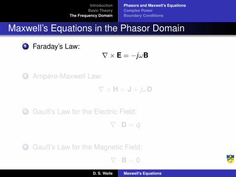
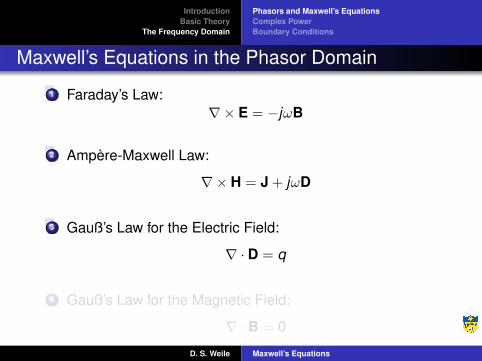
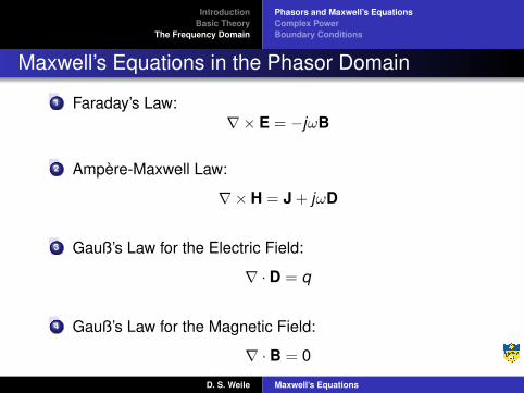
Maxwell’s Equations in the Phasor Domain
1 Faraday’s Law:∇× E = −jωB
2 Ampère-Maxwell Law:
∇× H = J + jωD
3 Gauß’s Law for the Electric Field:
∇ · D = q
4 Gauß’s Law for the Magnetic Field:
∇ · B = 0
D. S. Weile Maxwell’s Equations
IntroductionBasic Theory
The Frequency Domain
Phasors and Maxwell’s EquationsComplex PowerBoundary Conditions
Maxwell’s Equations in the Phasor Domain
1 Faraday’s Law:∇× E = −jωB
2 Ampère-Maxwell Law:
∇× H = J + jωD
3 Gauß’s Law for the Electric Field:
∇ · D = q
4 Gauß’s Law for the Magnetic Field:
∇ · B = 0
D. S. Weile Maxwell’s Equations
IntroductionBasic Theory
The Frequency Domain
Phasors and Maxwell’s EquationsComplex PowerBoundary Conditions
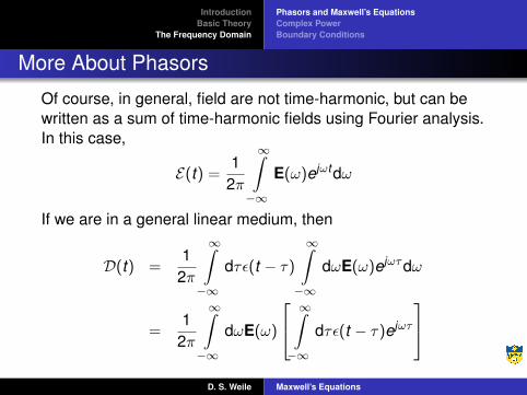
More About Phasors
Of course, in general, field are not time-harmonic, but can bewritten as a sum of time-harmonic fields using Fourier analysis.In this case,
E(t) = 12π
∞∫−∞
E(ω)ejωtdω
If we are in a general linear medium, then
D(t) =1
2π
∞∫−∞
dτε(t − τ)∞∫−∞
dωE(ω)ejωτdω
=1
2π
∞∫−∞
dωE(ω)
∞∫−∞
dτε(t − τ)ejωτ
D. S. Weile Maxwell’s Equations
IntroductionBasic Theory
The Frequency Domain
Phasors and Maxwell’s EquationsComplex PowerBoundary Conditions
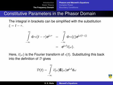
Constitutive Parameters in the Phasor Domain
The integral in brackets can be simplified with the substitutionξ = t − τ .
∞∫−∞
dτε(t − τ)ejωτ =
∞∫−∞
dτε(ξ)ejω(t−ξ)
= ejωt ε(ω).
Here, ε(ω) is the Fourier transform of ε(t). Substituting this backinto the definition of D gives
D(t) =∞∫−∞
ε(ω)E(ω)ejωtdω
D. S. Weile Maxwell’s Equations
IntroductionBasic Theory
The Frequency Domain
Phasors and Maxwell’s EquationsComplex PowerBoundary Conditions
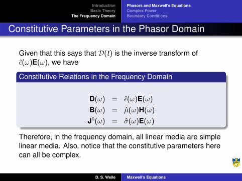
Constitutive Parameters in the Phasor Domain
Given that this says that D(t) is the inverse transform ofε(ω)E(ω), we have
Constitutive Relations in the Frequency Domain
D(ω) = ε(ω)E(ω)B(ω) = µ(ω)H(ω)
Jc(ω) = σ(ω)E(ω)
Therefore, in the frequency domain, all linear media are simplelinear media. Also, notice that the constitutive parameters herecan all be complex.
D. S. Weile Maxwell’s Equations
IntroductionBasic Theory
The Frequency Domain
Phasors and Maxwell’s EquationsComplex PowerBoundary Conditions
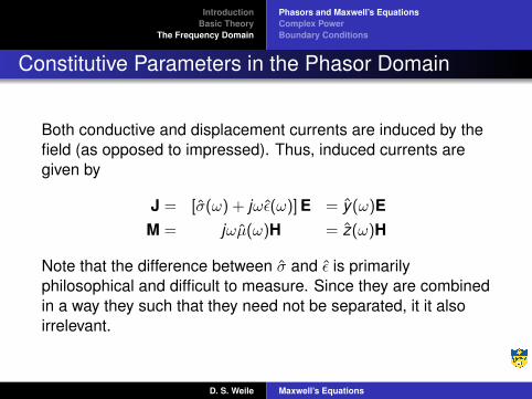
Constitutive Parameters in the Phasor Domain
Both conductive and displacement currents are induced by thefield (as opposed to impressed). Thus, induced currents aregiven by
J = [σ(ω) + jωε(ω)]E = y(ω)EM = jωµ(ω)H = z(ω)H
Note that the difference between σ and ε is primarilyphilosophical and difficult to measure. Since they are combinedin a way they such that they need not be separated, it it alsoirrelevant.
D. S. Weile Maxwell’s Equations

IntroductionBasic Theory
The Frequency Domain
Phasors and Maxwell’s EquationsComplex PowerBoundary Conditions
Final Form of the Curl Equations
Given all of these definitions, we can write the curl equations inthe form
−∇× E = z(ω)H + Mi
∇× H = y(ω)E + Ji
This is the most important form of these equations since itclearly separates sources from field effects.
D. S. Weile Maxwell’s Equations

IntroductionBasic Theory
The Frequency Domain
Phasors and Maxwell’s EquationsComplex PowerBoundary Conditions
Outline
1 Maxwell Equations, Units, and VectorsUnits and ConventionsMaxwell’s EquationsVector TheoremsConstitutive Relationships
2 Basic TheoryGeneralized CurrentDerivation of Poynting’s Theorem
3 The Frequency DomainPhasors and Maxwell’s EquationsComplex PowerBoundary Conditions
D. S. Weile Maxwell’s Equations

IntroductionBasic Theory
The Frequency Domain
Phasors and Maxwell’s EquationsComplex PowerBoundary Conditions
Poynting’s Theorem Revisited
Because S = E ×H, the computation of the Poynting vector isnonlinear, so more care is needed in bring it into the frequencydomain. To simplify matters, we can first look at how power iscomputed in circuit theory. Suppose
V(t) = Re{|V |ejφVejωt
}I(t) = Re
{|I|ejφIejωt
}Now
V(t)I(t) = |V ||I| cos(ωt + φV) cos(ωt + φI)
=12|V ||I| [cos(φV − φI) + cos(2ωt + φV + φI)]
D. S. Weile Maxwell’s Equations
IntroductionBasic Theory
The Frequency Domain
Phasors and Maxwell’s EquationsComplex PowerBoundary Conditions
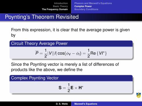
Poynting’s Theorem Revisited
From this expression, it is clear that the average power is givenby
Circuit Theory Average Power
P =12|V ||I| cos(φV − φI) =
12
Re {VI∗}
Since the Poynting vector is merely a list of differences ofproducts like the above, we define the
Complex Poynting Vector
S =12
E× H∗
D. S. Weile Maxwell’s Equations
IntroductionBasic Theory
The Frequency Domain
Phasors and Maxwell’s EquationsComplex PowerBoundary Conditions
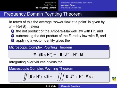
Frequency Domain Poynting Theorem
In terms of this the average “power flow at a point” is given byS = Re{S}. Taking
1 the dot product of the Ampère-Maxwell law with H∗, and2 subtracting the dot product of the Faraday law with E, and3 applying a vector identity gives the
Microscopic Complex Poynting Theorem
∇ · (E× H∗) = −E · Jt∗ − H∗ ·Mt
Integrating over volume givens the
Macroscopic Complex Poynting Theorem
©∫∫
(E× H∗) · dS = −∫∫∫
E · Jt∗ + H∗ ·Mtdv
D. S. Weile Maxwell’s Equations
IntroductionBasic Theory
The Frequency Domain
Phasors and Maxwell’s EquationsComplex PowerBoundary Conditions
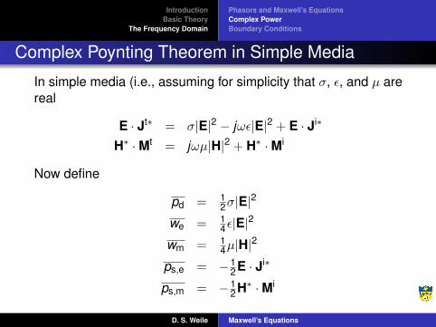
Complex Poynting Theorem in Simple Media
In simple media (i.e., assuming for simplicity that σ, ε, and µ arereal
E · Jt∗ = σ|E|2 − jωε|E|2 + E · Ji∗
H∗ ·Mt = jωµ|H|2 + H∗ ·Mi
Now define
pd = 12σ|E|
2
we = 14ε|E|
2
wm = 14µ|H|
2
ps,e = −12E · Ji∗
ps,m = −12H∗ ·Mi
D. S. Weile Maxwell’s Equations

IntroductionBasic Theory
The Frequency Domain
Phasors and Maxwell’s EquationsComplex PowerBoundary Conditions
Complex Poynting Theorem in Simple Media
Finally, defining pf = ∇ · S, we can finally interpret Poynting’sTheorem
Poynting’s Theorem Interpreted
ps = pf + pd + 2jω(wm − we)
All but the last term represent real average power flow. The lastterm represents reactive power, that is, the movement of powerback and forth between electric and magnetic form. How do Iknow this?Finally, the integral form of this theorem is trivial to derive andinterpret.
D. S. Weile Maxwell’s Equations

IntroductionBasic Theory
The Frequency Domain
Phasors and Maxwell’s EquationsComplex PowerBoundary Conditions
Outline
1 Maxwell Equations, Units, and VectorsUnits and ConventionsMaxwell’s EquationsVector TheoremsConstitutive Relationships
2 Basic TheoryGeneralized CurrentDerivation of Poynting’s Theorem
3 The Frequency DomainPhasors and Maxwell’s EquationsComplex PowerBoundary Conditions
D. S. Weile Maxwell’s Equations
IntroductionBasic Theory
The Frequency Domain
Phasors and Maxwell’s EquationsComplex PowerBoundary Conditions
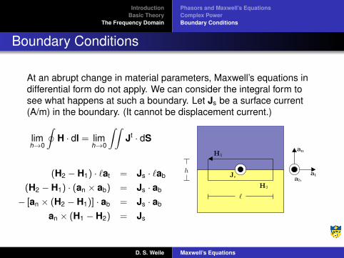
Boundary Conditions
At an abrupt change in material parameters, Maxwell’s equations indifferential form do not apply. We can consider the integral form tosee what happens at such a boundary. Let Js be a surface current(A/m) in the boundary. (It cannot be displacement current.)
limh→0
∮H · dl = lim
h→0
∫∫Jt · dS
(H2 − H1) · `at = Js · `ab
(H2 − H1) · (an × ab) = Js · ab
− [an × (H2 − H1)] · ab = Js · ab
an × (H1 − H2) = Js
an
atab
Jsh
!
H1
H2
D. S. Weile Maxwell’s Equations

IntroductionBasic Theory
The Frequency Domain
Phasors and Maxwell’s EquationsComplex PowerBoundary Conditions
General Boundary Conditions
Faraday’s Law works the same way. General boundaryconditions can be derived from the Gauss Laws by looking at asmall volume. The results are
General Boundary Conditions
an × (H1 − H2) = Js
(E1 − E2)× an = Ms
an · (D1 − D2) = qS
an · (B1 − B2) = qm,S
D. S. Weile Maxwell’s Equations

IntroductionBasic Theory
The Frequency Domain
Phasors and Maxwell’s EquationsComplex PowerBoundary Conditions
Finite Conductivity Boundary
If neither material has infinite conductivity, there can be nocharge in the boundary. This leads to the
Dielectric Boundary Conditions
an × (H1 − H2) = 0an × (E1 − E2) = 0an · (D1 − D2) = 0an · (B1 − B2) = 0
D. S. Weile Maxwell’s Equations
IntroductionBasic Theory
The Frequency Domain
Phasors and Maxwell’s EquationsComplex PowerBoundary Conditions
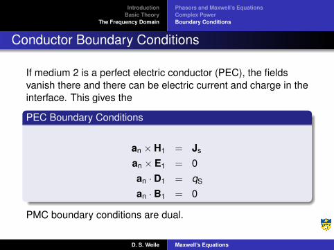
Conductor Boundary Conditions
If medium 2 is a perfect electric conductor (PEC), the fieldsvanish there and there can be electric current and charge in theinterface. This gives the
PEC Boundary Conditions
an × H1 = Js
an × E1 = 0an · D1 = qS
an · B1 = 0
PMC boundary conditions are dual.
D. S. Weile Maxwell’s Equations