Maximum Probability Domains From Quantum Monte … · Maximum Probability Domains From Quantum...

Maximum Probability Domains From QuantumMonte Carlo Calculations*

ANTHONY SCEMAMA,1 MICHEL CAFFAREL,2 ANDREAS SAVIN3

1CERMICS, Ecole Nationale des Ponts et Chaussées, 6 et 8 avenue Blaise Pascal,Cité Descartes—Champs sur Marne, 77455 Marne la Vallée Cedex 2, France

2Laboratoire de Chimie et Physique Quantiques, CNRS-UMR 5626, IRSAMC UniversitéPaul Sabatier, 118 route de Narbonne, 31062 Toulouse Cedex, France

3Laboratoire de Chimie Théorique, CNRS-UMR 7616, Université Paris Pierre et Marie Curie,Case 137, 4 place Jussieu, 75252 Paris Cedex 05, France

Received 31 March 2006; Revised 27 June 2006; Accepted 29 June 2006DOI 10.1002/jcc.20526

Published online in Wiley InterScience (www.interscience.wiley.com).

Abstract: Although it would be tempting to associate the Lewis structures to the maxima of the squared wave function|�|2, we prefer in this paper the use of domains of the three-dimensional space, which maximize the probability ofcontaining opposite-spin electron pairs. We find for simple systems (CH4, H2O, Ne, N2, C2H2) domains comparable tothose obtained with the electron localization function (ELF) or by localizing molecular orbitals. The different domains wedefine can overlap, and this gives an interesting physical picture of the floppiness of CH+

5 and of the symmetric hydrogenbond in FHF−. The presence of multiple solutions has an analogy with resonant structures, as shown in the trans-bentstructure of Si2H2. Correlated wave functions were used (MCSCF or Slater-Jastrow) in the Variational Quantum MonteCarlo framework.

© 2006 Wiley Periodicals, Inc. J Comput Chem 28: 442–454, 2007

Key words: chemical bond; maximum probability domains; electron localization function; Quantum Monte Carlo;electron pair

Introduction

Lewis’ concept of electron sharing producing electron pairs wasextremely fruitful in chemistry, but its translation to quantummechanics is not self-evident. Lewis himself was pessimistic.1 In1916, quantum mechanics was still in an embryonic stage, and Lewisfound it “hardly likely that much progress can be made” using it.

From the present perspective, the obstacle is the connectionbetween the high dimensionality of quantum mechanics (of thesquared wave function, |�|2) and the three-dimensional space ofthe molecular structure. One approach is to reduce the dimen-sionality by averaging over the positions of all electrons exceptone.2 One can also use other three-dimensional functions such aslocalized orbitals,3 the electron localization function,4 (ELF) ordecompositions like in population analysis.5

In Variational Quantum Monte Carlo (VMC), one works directlywith |�|2. Thus, some of the techniques just mentioned are applica-ble, but inadequate. In this paper, we will try to show that there is atool yielding an image close to that of Lewis and which is generallyapplicable to quantum mechanical methods, including VMC.

In fact, Lewis was much concerned about the spatial arrangementof valence electrons. In his paper,1 he starts with a “cubical atom,”the valence electrons being able to choose positions at the corners

of a cube. This allows a maximum of eight electrons around anatom. As Lewis goes on with his argumentation, he tends to giveit up due to “triple bonds for which the cubical structure offers nosimple representation.” Another problematic case he discusses isthat of the lithium atom, where the octet rule (term later introducedby Langmuir6) is not satisfied. He recognizes that in such a case“the pair of electrons forms the stable group.” Finally he suggeststhat for the C C bond the pairs of electrons around a carbon atommight be arranged tetrahedrally. Later, when the concept of electronspin was introduced, Linnett7 considers that for each spin separatelyelectrons arrange themselves tetrahedrally around the nucleus, andthat the two tetrahedra are kept apart.

From our present perspective, |�|2 controls the spatial dis-tribution of electrons. This has been exploited to return to thethree-dimensional structure of molecules. It was suggested8, 9 tosimply select the most probable arrangement of valence electrons,

*Dedicated to Professor Hans Georg von Schnering for his 75th birthday.

Correspondence to: A. Savin; e-mail: [email protected]

Contract/grant sponsor: Ministère Français de l’Enseignement Supérieuret de la Recherche Action Concertáe Incitative (ACI): “Simulation Molécu-laire.”

© 2006 Wiley Periodicals, Inc.

Maximum Probability Domains From Quantum Monte Carlo Calculations 443

Figure 1. Positions of the electron pairs at a maximum of the squaredsingle determinant wave function, in the water molecule. The positionsof the electron pairs (one spin-up and one spin-down at the same posi-tion) are shown as blue spheres. The locations of the hydrogen nuclei arerepresented as transparent white spheres, and that of the oxygen nucleusas a transparent red sphere. The electron pairs are connected with sticksto show the tetrahedral configuration.

i.e. the positions of the electrons that maximize |�|2. For example,in the sp3 carbon atom, Artmann8 shows that |�|2 is maximal whenthe electrons are localized at the vertices of a tetrahedron. In fact,it is quite easy to show that for perfectly localized orbitals, φi, themaximum of the Slater determinant built from them corresponds tothe arrangement where the electron pairs occupy the positions where|φi| take their largest value. (φi are perfectly localized orbitals when∫ |φi(r)|2|φj(r)|2dr = 0, i �= j, or if φi(r) �= 0, φj(r) = 0 for allj �= i). Note that quantum mechanics allows two electrons to occupythe same infinitesimal volume element as long as they have oppositespins. In Figure 1 the positions of the electron pairs at a maximumof the single determinant (Hartree-Fock) wave function are shownfor the water molecule.

When the single-determinant approximation is overcome (cor-relation is taken into account), we find that electrons of a pair tendto separate: The maximum of the single-determinant wave functionis not a maximum of the correlated wave function. The maximumis achieved when the electrons of a pair occupy different positionsin space. We see in Figure 2 that in the water molecule the elec-trons of the O H bonds separate along the bonds, “pre-dissociate,”while the electrons of the lone pairs separate in a direction perpen-dicular to the tetrahedral axis, similar to Figure 5 in Lewis’ paper.1

Fulde10 also noticed such effects in the correlated pair distributions.There are different equivalent maxima obtained by permutation ofspins.

We now come to another concept of Lewis, namely that of tau-tomerism. Lewis assumes that in a given substance, “it must not be

assumed that all of the molecules are in the same state, but rather thatsome are highly polar, some almost nonpolar, and others representall gradations between the two.” For Lewis, a nonpolar molecule isone “in which the electrons belonging to the individual atom are heldby such constraints that they do not move far from their normal posi-tions, while in the polar molecule the electrons, being more mobile,so move as to separate the molecule into positive and negative parts.”In the language of quantum mechanics, one could say that there is aprobability for a given arrangement of electrons obtained from |�|2.In this context one can ask about the relevance of considering onlythe highest maximum of |�|2. For example one can find anothermaximum corresponding to a structure (Fig. 3) resembling Lewis’cubical atom.1 The value of |�|2 at this maximum is close to thevalue at the maximum corresponding to the arrangement shown inFigure 2. Another way to look at this arrangement is that of twodisplaced tetrahedra, as proposed by Linnett7 (Fig. 4).

Also, as |�|2 is a probability density, the probability of havingthe given electron arrangement can be low if |�|2 is sharply peakedaround the maximum and the values of |�|2 close to the maximumare low. The electron arrangement can be of little significance ifthere are several other positions yielding also high values of |�|2.Thus, instead of searching for the positions of electrons which max-imize |�|2 it might be more relevant to investigate the regions ofspace where the probability of finding a pair of electrons is large. Wewill follow in the present paper this path, searching for the regionsof space � where the probability P� to find pairs of electrons ofopposite spins is maximal.

Figure 2. Positions of the electron pairs at a maximum of the squaredcorrelated wave function, in the water molecule. The positions of thespin-up electrons are shown as blue spheres and those of the spin-downelectrons are shown as green spheres. The location of the hydrogennuclei are represented as transparent white spheres, and that of the oxy-gen nucleus as a transparent red sphere. Sticks join the electrons of apair.

Journal of Computational Chemistry DOI 10.1002/jcc

444 Scemama, Caffarel, and Savin • Vol. 28, No. 1 • Journal of Computational Chemistry

Figure 3. Positions of the electron pairs at another maximum of thesquared correlated wave function in the water molecule. The positionsof the spin-up electrons are shown as blue spheres and those of thespin-down electrons are shown as green spheres. The location of thehydrogen nuclei are represented as transparent white spheres, and that ofthe oxygen nucleus as a transparent red sphere. Sticks join the electronsof a pair, and a cube has been added to the figure to show that the electronpairs almost form Lewis’ cubical atom.1

Before going on with specific examples, a few remarks:

• We consider here only pairs of electrons with opposite spins asthis is assumed to be the quantum mechanical equivalent to Lewis’electron pairs.

• It is natural to find several regions � as they correspond todifferent bonds or lone pairs.

• We expect to obtain regions that correspond to those where molec-ular orbitals localize. However, the method we use is not restrictedto a given type of wave function. In particular, it is not restricted tosingle Slater determinants. Within VMC, we have considered inthe following explicitly correlated wave functions.

• As we define spatial regions, we define sharp borders. This is tobe opposed to localized orbitals that extend over the whole spaceand are only dominant in some region of space.

• The regions of space we define are not basins as it is done in thetheory of Atoms in Molecules2 or for the ELF,11 although weexpect some resemblance of our �s with the latter.

• The different �s we consider may overlap in contrast with thebasins above, or with Daudel and coworkers’ loges.12 The lat-ter correspond to a most favorable partition of space, while wefind multiple solutions of our maximization problem. Differentapproaches to interpret chemical bonding may have differentadvantages, and may be used with more or less success in adifferent context. Allowing the domains to overlap may be con-ceptually less satisfying than partitioning of space (as it also

happens with basins), but overlapping may allow, if necessary,to reduce fluctuation of particles between domains.

• As it is common practice to look at the average number of elec-trons in a region of space (population), we will also present thisnumber for �. It is not an integer, as opposed to the number ofelectrons associated with the probability used to construct�. Notethat there is no special reason why the average population and thenumber of electrons for which the probability has been computedshould be identical. However, in practice these two numbers arefound to be quite close. Moreover, the population counts alsoelectrons of parallel spins and there are situations where thereare more or less than the number of electrons considered whenobtaining �.

The technical details of our calculations are presented in appen-dices. The first one presents the calculation of the probabilities in �,and the second one presents the algorithm for optimizing the regionsof space so as to obtain the �s. The data concerning the geometries,basis functions, and Jastrow factors will be provided upon request.Before pursuing with applications, we would like to mention somelimitations of our approach.

• The analysis is as good as the wave function we use. VMC allowssome flexibility in its choice but the ansatz is also subject toprejudice. In the results presented in this paper, the inclusion ofcorrelation has only little changed the �s and the corresponding

Figure 4. Positions of the electron pairs at the same maximum as inFigure 3 of the squared correlated wave function in the water molecule.The positions of the spin-up electrons are shown as blue spheres, thoseof the spin-down electrons are shown as green spheres, those of thehydrogen nuclei as transparent white spheres, and that of the oxygennucleus as a transparent red sphere. The spin-up and spin-down electronsare both connected together with sticks. Remark that the electrons ofsame spin are placed at the vertices of a tetrahedron, as suggested byLinnett.7



Figure 5. A domain maximizing the probability of finding two electronswith opposite spins, in CH4.

probabilities, despite the noticeable separation of the electrons inthe maxima of |�|2.

• The VMC method performs an exploration of |�|2 for a finitenumber of electron arrangements (configurations). Some infor-mation is lost in particular in the regions of low density, asthese are rarely explored by VMC. This can give slightly toolow populations or slightly too compact domains.

• The convergence criterion of the domain search algorithm mayalso be a source of error. For instance, if the optimal domainis not completely reached, � can have an overlap region withanother domain, which can in some cases be reduced by furtheroptimization.

• � is constructed from a union of small boxes, of size adaptedto the number of configurations, which in our case have edgesof ∼0.1 atomic units, which is also typical for other calculationsanalyzing the chemical bond. In our figures we have chosen notto use interpolation. One one hand, it produces some roughnessof surfaces shown. However, on the other hand, it gives somevisualization of the quality of our calculation.

We would like to mention that some work has already been donefor atoms and linear molecules using single determinant wave func-tions,13–15 as well as correlated wave functions.16 This paper is thefirst in which we present nonlinear molecules.

Applications

Simple Systems

CH4. Our first example is the methane molecule, where theexpected results are found: Each valence domain contains one pro-ton, and the electron pairs symmetrically partition the valence space(Fig. 5) in a way that is very similar to that obtained by the topo-

logical analysis of ELF displayed in Figure 6, and also analogousto domains where orbitals would localize.

Each � is populated by 2.0 electrons. The spin-independentprobabilities of finding one, two, and three electrons inside an opti-mal domain corresponding to the C H bond are respectively 0.21,0.55, and 0.19 (see Table 1). The spin-dependent probability of find-ing two electrons with opposite spins is P(2, 1) = 0.51 (where the“1” in the notation “P(2, 1)” stands for the singlet coupling). Forthe same population inside the domain, one can compute the prob-abilities one would obtain if the electrons were independent. Thedifference of the probabilities with those obtained with independentparticles shows the quantum effects. The differences with the prob-abilities of finding independent electrons (in a statistical sense, bya binomial distribution, and not constructed from a Slater determi-nant, cf. Appendix A) are −0.06, 0.25, and −0.01. A clear quantumchemical enhancement of the probability of finding two electronsinside the domain is observed. However, this is not the case for theprobabilities of finding one or three electrons. In this latter case, thesituation is similar to what would happen with classical particlesignoring the Pauli principle and considered as statistically indepen-dent. The probabilities were also calculated in the ELF basin, andall the values are practically equal to those in �.

Note that the basins of a topological analysis are defined as apartition of space, so the overlap of the basins is impossible bydefinition. Here, nothing prevents the domains from intersecting,and one can observe a very small overlap between two adjacentdomains. This seems to be an artifact of the algorithm, as using asymmetry-based partition of the space yields probabilities, whichare the same within our accuracy.

H2O. Similar to that in CH4, we obtain a structure with four domainsplaced at the corners of a tetrahedron with a small overlap. Theycorrespond to the O H bonds and the lone pairs. One of each of

Figure 6. A basin of the electron localization function (ELF) corre-sponding to a C H bond in CH4.



Table 1. Spin-Independent Probabilities P(ν) of Finding ν Electrons, Spin-Dependent Probability P(2, 1) ofFinding One Opposite-Spin Electron Pair, and Population in Each One of the Domains � of CH4, H2O, Ne,FHF− In and Out of Equilibrium, the Cs and C2v Structures of CH+

5 .

P(0) P(1) P(2) P(3) P(4) P(2, 1) Pop.

C H bond in CH4 0.02 0.21 0.55 0.19 0.03 0.51 2.0(−0.09) (−0.06) (0.25) (−0.01) (−0.06)

O H bond in H2O 0.04 0.26 0.46 0.20 0.04 0.39 1.9(−0.07) (−0.02) (0.15) (0.00) (−0.04)

Lone pair in H2O 0.05 0.26 0.42 0.21 0.05 0.39 2.0(−0.06) (−0.01) (0.12) (0.01) (−0.04)

Lone pair in Ne 0.06 0.26 0.39 0.22 0.06 0.30 2.0(−0.05) (−0.01) (0.09) (0.02) (−0.03)

F H bond in FHF− 0.06 0.27 0.39 0.21 0.06 0.30 2.0(−0.07) (0.00) (0.11) (0.02) (−0.03)

Three-center bond in CH+5 Cs symmetry 0.02 0.22 0.52 0.20 0.03 0.47 2.0

(−0.08) (−0.05) (0.22) (0.00) (−0.06)

Three-center bond in CH+5 C2v symmetry 0.03 0.24 0.54 0.16 0.02 0.50 1.9

(−0.09) (−0.04) (0.24) (−0.03) (−0.06)

�P(ν), the differences with probabilities in the case of statistically independent particles, are given in brackets. Alldomains maximize P(2, 1).

these domains is presented in Figure 7. The �s corresponding tolone pairs and bonds are naturally not equivalent. The populationin both domains is 2.0, and the probabilities are given in Table 1 aswell as the differences of probabilities with the case of independentparticles. As for methane, the quantum mechanical enhancement ofthe probabilities is significant for electron pairs.

Ne. As spherical symmetry is not imposed in the domain searchalgorithm, the valence of the neon atom can be described similar toCH4 and H2O by four domains containing each one spin-up and one

Figure 7. Domains maximizing the probability of finding two electronswith opposite spins, in H2O. The yellow domain represents the lone pairdomain and the transparent blue domain corresponds to the O H bond.

spin-down electron. These four domains are equivalent among them,but not unique. Figure 8 shows a domain maximizing the probabilityof finding two electrons with opposite spins. Each domain containson average 2.0 electrons, and the probabilities are given in Table 1.

The group of four domains can be arbitrarily rotated around thenucleus, in contrast to CH4 and H2O, where the orientation is fixedby the nuclei. However, in the HF molecule (not shown) the protondefines only one axis, and the three domains representing the lonepairs of the F atom can freely rotate around it. We can again noticean enhancement of P(2) due to quantum mechanical effects.

Figure 8. A domain maximizing the probability of finding two electronswith opposite spins (yellow), in the neon atom. The position of thenucleus is represented by a red sphere.



Figure 9. Domains maximizing the probability of finding one (yellowand green), and three (red) antiparallel electron pairs (three spins up andthree spins down) in N2. The red domain was made transparent to showthe positions of the two nuclei (violet spheres). One can distinguish herethe σ and π regions of the N N bond.

As the ELF respects by definition the symmetry of the wavefunction, ELF can see only an average of the “resonant” forms. Incases where there is only one structure, the borders of a domaincorrespond approximately to the separatrix of the basins of ELF,as in CH4 for example. If there are several equivalent maximumprobability domains, ELF will produce an average picture. In theneon atom, the average produced by ELF produces a spherical shell,and this one will include both the maximum probability domains aswell as their borders. As a result, instead of showing a maximumlocalization (≈1.0), ELF presents a lower value (≈0.8).

N2. N2 is a textbook example for the triple bond. Nevertheless, thetopological analysis of the ELF gives a population close to four elec-trons in the N N bond, which does not correspond to the commonLewis structure.17 Here, we searched for the domains maximiz-ing the probabilities of finding three up and three down electronsbetween the two nuclei, following the traditional σ/π interpreta-tion of the bond. The �s obtained are shown in Figure 9. The greendomain corresponds to the σ region of the N N bond, and the yellowdomain describes one of the lone pairs. The red domain maximizesthe probability of finding three up and three down electrons. Thesurface has been cut so as to make the σ (green) domain visible.

The probabilities are given in Table 2. For the domain associatedto the lone pair, there is a noticeable quantum mechanical enhance-ment of the probability to find three electrons. This may explainwhy the ELF basins describing the lone pairs are too populated.

However, there is another solution showing up when searchingfor an � corresponding to a pair of electrons. This is shown inFigure 10. It corresponds to one of the three banana bonds. As forthe lone pairs of HF, the group of three domains can freely rotatealong the molecular axis.

Notice that there is again another solution for the �s corre-sponding to electron pairs, which correspond to π bonds. Thesecan freely rotate around the molecular axis. They are not shown asa figure, but one can imagine their shape by removing the σ domainfrom the � corresponding to the triple bond and by dividing theremaining part by a plane containing the molecular axis.

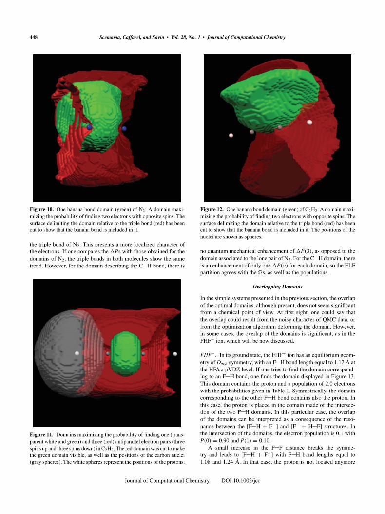
C2H2. The electronic structure of acetylene is similar to the struc-ture of N2. The lone pairs in N2 are replaced by C H bonds inacetylene. Here, one finds domains where the populations agree withthe populations of the ELF basins. The corresponding domains aredisplayed in Figure 11. One banana bond domain is presented inFigure 12. Because of the cylindrical symmetry, the group of threebanana bond domains can freely rotate along the molecular axis. Asfor N2, one finds σ and π domains with values of P(ν) similar tothose of the banana bond domains.

The values of the maximal probabilities for the C H and C Cbonds (Table 3) are slightly higher than for the lone pair and for

Table 2. Spin-Independent Probabilities P(ν) of Finding ν Electrons, Spin-Dependent Probability P(2, 1) ofFinding One Opposite-Spin Electron Pair, and Population in Each One of the Domains � of N2.

P(0) P(1) P(2) P(3) P(4) P(5) P(6) P(7) P(8) P(2, 1) Pop.

Lone Pair 0.04 0.25 0.46 0.20 0.04 0.00 0.40 2.0(−0.01) (−0.02) (0.17) (0.12) (−0.05) (−0.02)

σ bond 0.07 0.28 0.39 0.20 0.05 0.01 0.29 1.9(−0.06) (0.00) (0.09) (0.02) (−0.03) (−0.02)

π bond 0.07 0.28 0.37 0.21 0.06 0.01 0.28 2.0(−0.05) (0.00) (0.08) (0.02) (−0.02) (−0.02)

Banana bond 0.06 0.27 0.39 0.21 0.06 0.01 0.29 2.0(−0.06) (0.00) (0.10) (0.02) (−0.03) (−0.02)

Triple bond 0.00 0.03 0.11 0.24 0.31 0.21 0.08 5.9(−0.02) (−0.04) (−0.03) (0.05) (0.09) (0.04) (−0.03)

�P(ν), the differences with probabilities in the case of statistically independent particles, are given in brackets. The lonepair domain and the σ bond domain maximize P(2, 1) and the triple bond domain maximizes P(6, 1), the spin-dependentprobability of finding three up electrons and three down electrons. The banana bond domain maximizes P(2, 1).



Figure 10. One banana bond domain (green) of N2: A domain maxi-mizing the probability of finding two electrons with opposite spins. Thesurface delimiting the domain relative to the triple bond (red) has beencut to show that the banana bond is included in it.

the triple bond of N2. This presents a more localized character ofthe electrons. If one compares the �Ps with those obtained for thedomains of N2, the triple bonds in both molecules show the sametrend. However, for the domain describing the C H bond, there is

Figure 11. Domains maximizing the probability of finding one (trans-parent white and green) and three (red) antiparallel electron pairs (threespins up and three spins down) in C2H2. The red domain was cut to makethe green domain visible, as well as the positions of the carbon nuclei(gray spheres). The white spheres represent the positions of the protons.

Figure 12. One banana bond domain (green) of C2H2: A domain maxi-mizing the probability of finding two electrons with opposite spins. Thesurface delimiting the domain relative to the triple bond (red) has beencut to show that the banana bond is included in it. The positions of thenuclei are shown as spheres.

no quantum mechanical enhancement of �P(3), as opposed to thedomain associated to the lone pair of N2. For the C H domain, thereis an enhancement of only one �P(ν) for each domain, so the ELFpartition agrees with the �s, as well as the populations.

Overlapping Domains

In the simple systems presented in the previous section, the overlapof the optimal domains, although present, does not seem significantfrom a chemical point of view. At first sight, one could say thatthe overlap could result from the noisy character of QMC data, orfrom the optimization algorithm deforming the domain. However,in some cases, the overlap of the domains is significant, as in theFHF− ion, which will be now discussed.

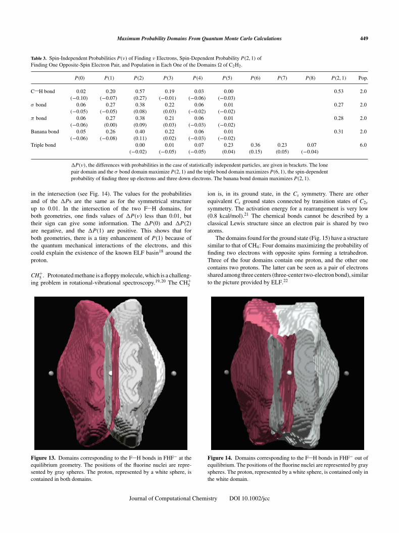
FHF−. In its ground state, the FHF− ion has an equilibrium geom-etry of D∞h symmetry, with an F H bond length equal to 1.12 Å atthe HF/cc-pVDZ level. If one tries to find the domain correspond-ing to an F H bond, one finds the domain displayed in Figure 13.This domain contains the proton and a population of 2.0 electronswith the probabilities given in Table 1. Symmetrically, the domaincorresponding to the other F H bond contains also the proton. Inthis case, the proton is placed in the domain made of the intersec-tion of the two F H domains. In this particular case, the overlapof the domains can be interpreted as a consequence of the reso-nance between the [F H + F−] and [F− + H F] structures. Inthe intersection of the domains, the electron population is 0.1 withP(0) = 0.90 and P(1) = 0.10.

A small increase in the F F distance breaks the symme-try and leads to [F H + F−] with F H bond lengths equal to1.08 and 1.24 Å. In that case, the proton is not located anymore



Table 3. Spin-Independent Probabilities P(ν) of Finding ν Electrons, Spin-Dependent Probability P(2, 1) ofFinding One Opposite-Spin Electron Pair, and Population in Each One of the Domains � of C2H2.

P(0) P(1) P(2) P(3) P(4) P(5) P(6) P(7) P(8) P(2, 1) Pop.

C H bond 0.02 0.20 0.57 0.19 0.03 0.00 0.53 2.0(−0.10) (−0.07) (0.27) (−0.01) (−0.06) (−0.03)

σ bond 0.06 0.27 0.38 0.22 0.06 0.01 0.27 2.0(−0.05) (−0.05) (0.08) (0.03) (−0.02) (−0.02)

π bond 0.06 0.27 0.38 0.21 0.06 0.01 0.28 2.0(−0.06) (0.00) (0.09) (0.03) (−0.03) (−0.02)

Banana bond 0.05 0.26 0.40 0.22 0.06 0.01 0.31 2.0(−0.06) (−0.08) (0.11) (0.02) (−0.03) (−0.02)

Triple bond 0.00 0.01 0.07 0.23 0.36 0.23 0.07 6.0(−0.02) (−0.05) (−0.05) (0.04) (0.15) (0.05) (−0.04)

�P(ν), the differences with probabilities in the case of statistically independent particles, are given in brackets. The lonepair domain and the σ bond domain maximize P(2, 1) and the triple bond domain maximizes P(6, 1), the spin-dependentprobability of finding three up electrons and three down electrons. The banana bond domain maximizes P(2, 1).

in the intersection (see Fig. 14). The values for the probabilitiesand of the �Ps are the same as for the symmetrical structureup to 0.01. In the intersection of the two F H domains, forboth geometries, one finds values of �P(ν) less than 0.01, buttheir sign can give some information. The �P(0) and �P(2)

are negative, and the �P(1) are positive. This shows that forboth geometries, there is a tiny enhancement of P(1) because ofthe quantum mechanical interactions of the electrons, and thiscould explain the existence of the known ELF basin18 around theproton.

CH+5 . Protonated methane is a floppy molecule, which is a challeng-

ing problem in rotational-vibrational spectroscopy.19, 20 The CH+5

Figure 13. Domains corresponding to the F H bonds in FHF− at theequilibrium geometry. The positions of the fluorine nuclei are repre-sented by gray spheres. The proton, represented by a white sphere, iscontained in both domains.

ion is, in its ground state, in the Cs symmetry. There are otherequivalent Cs ground states connected by transition states of C2v

symmetry. The activation energy for a rearrangement is very low(0.8 kcal/mol).21 The chemical bonds cannot be described by aclassical Lewis structure since an electron pair is shared by twoatoms.

The domains found for the ground state (Fig. 15) have a structuresimilar to that of CH4: Four domains maximizing the probability offinding two electrons with opposite spins forming a tetrahedron.Three of the four domains contain one proton, and the other onecontains two protons. The latter can be seen as a pair of electronsshared among three centers (three-center two-electron bond), similarto the picture provided by ELF.22

Figure 14. Domains corresponding to the F H bonds in FHF− out ofequilibrium. The positions of the fluorine nuclei are represented by grayspheres. The proton, represented by a white sphere, is contained only inthe white domain.



Figure 15. CH+5 in its ground state. The domain corresponding to the

three-center bond is shown with dots. A domain relative to a C H bondis displayed in order to show the overlap between the two domains.

The CH+5 ion in the transition state is represented in Figure 16

and the probabilities are given in Table 1. The optimal domains areanalogous to those found for the ground state, but one of the protonsparticipating to the three-center bond has moved towards the side ofthe domain in the intersection with the neighboring domain. Nowwe have two equivalent domains containing two protons, one protonbeing shared by these two domains. The description is similar to thatof FHF−.

The present description of the bonds agrees with the very flux-ional character of the molecule. The structure of the bondingdomains does not change when going from the Cs to the C2v confor-mation. Here, we can see the system as a central carbon nucleus, twocore electrons with opposite spins, and five protons moving easily ina fluid of eight valence electrons arranged as four pairs of oppositespins.

Figure 16. CH+5 in the transition state. The proton is contained in the

intersection of the transparent and the dotted domains.

Degenerate Structures—Si2H2

In contrast to C2H2, the most stable conformation of Si2H2 has abutterfly structure. However, there exists a local minimum that isclosely related to the structure of C2H2. For a recent study of thistrans-bent structure of Si2H2, see refs. 23–25.

A domain corresponding to the Si H bond was found, with apopulation of 1.9 electrons. The probabilities are given in Table 4.Between the two silicon atoms, we found a domain correspondingto a distorted triple bond populated by 5.8 electrons. The distortionis associated to the push of the Si H bond as shown in Figure 17.

Distorted banana bonds of Si2H2 were also found (Fig. 18). Asopposed to C2H2, they cannot freely rotate, but there exists only twoways of assigning them, which are related by the inversion symmetryoperation. These two structures can be viewed as resonant forms (seebottom of Fig. 18). The probabilities are given in Table 4.

Table 4. Spin-Independent Probabilities P(ν) of Finding ν Electrons, Spin-Dependent Probability P(2, 1) ofFinding One Opposite-Spin Electron Pair, and Population in Each One of the Domains � of Si2H2.

P(0) P(1) P(2) P(3) P(4) P(5) P(6) P(7) P(8) P(2, 1) Pop.

Si H bond 0.02 0.22 0.59 0.15 0.02 0.56 1.9(−0.11) (−0.06) (0.30) (−0.03) (−0.06)

Banana bond 0.07 0.27 0.38 0.21 0.06 0.01 0.28 2.0(−0.06) (0.02) (0.10) (0.02) (−0.02) (−0.02)

Two equivalent banana bonds 0.07 0.28 0.38 0.20 0.05 0.01 0.26 1.9(−0.06) (0.01) (0.11) (0.04) (−0.03) (−0.02)

Triple bond 0.01 0.03 0.12 0.25 0.29 0.19 0.08 5.8(−0.03) (−0.05) (−0.02) (0.07) (0.11) (0.04) (−0.02)

�P(ν), the differences with probabilities in the case of statistically independent particles, are given in brackets. The Si Hbond and the banana bond domains maximize P(2, 1). The triple bond domain maximizes P(6, 1).



Figure 17. Trans-bent structure of Si2H2: The optimal domains cor-respond to the Si H bond (white) and a distorted Si Si triple bond(blue). The domains have been cut along the molecular plane to showthe distorted character of the triple bond domain.

The optimized domains do not agree with the ELF partition,23

where four equivalent basins with fractional populations are found(Fig. 19). The two resonant forms may explain the ELF partition. Asremarked for N2, ELF shows an average of the resonant forms. Thesuperimposition of the domain corresponding to the “single bond”

Figure 18. Banana bonds of Si2H2. The domains were cut in a planeorthogonal to the Si Si axis in order to show their overlap. The tworesonant structures are displayed at the bottom of the figure, and thedomains displayed correspond to the resonant structure on the left.

Figure 19. Isosurfaces of the electron localization function (ELF) inthe trans-bent structure of Si2H2. The isosurface ELF = 0.88 is dis-played in transparent yellow, and the isosurface ELF = 0.94 (in fullyellow) shows the positions of the maxima.

of one resonant structure and those corresponding to the “doublebond” of the other resonant structure decreases the ELF separationbetween the two domains describing the double bond, so that thedouble bonds of the upper part of the figure will give raise only totwo localization domains, slightly separated by the molecular plane.Close to the plane perpendicular to it containing the silicon nuclei,we can see the borders of maximum probability domains in bothstructures, and thus expect that the separation in ELF will be moreclear.

Summary

Quantum mechanics requires the delocalization of the electron pairs,leading us to the definition of possibly overlapping domains. Theregions maximizing the probability of finding a given number ofpairs of electrons with opposite spins were found, and often domainsresembling basins of the ELF or domains of orbital localization wereobtained. Simple cases where four electron pairs share the molecularspace were described (CH4, H2O, Ne). The domains of acetyleneare very similar to the ELF basins, and although N2 has an electronicstructure very close to that of C2H2, its domains are slightly differentfrom the ELF basins, and the triple bond can easily be found withthe presented method.

A case that cannot be represented by basins is FHF−, wherethe overlap of the domains is chemically relevant: The protontakes advantage of both F H bonds of the two resonant structures.Another interesting case of overlapping domains is CH+

5 , where theelectronic structure is fixed, and the protons can move easily in the“fluid” made of the four electron pairs.

In some situations, the degeneracy of the optimal domains is self-evident (the four electron pairs of the Neon atom, or the three banana



bonds of acetylene). Nevertheless, there exists some structureswhere this degeneracy is less obvious, as in Si2H2.

Acknowledgments

It is our pleasure to dedicate this paper to Professor H. G. vonSchnering (Stuttgart) on his 75th birthday for continuously sup-porting and contributing to the methods helping to understand thechemical bond.

A. Scemama thanks the ACI: “Simulation Moléculaire” for apostdoctoral position. We also would like to acknowledge interest-ing discussions with Roland Assaraf (Université Pierre et MarieCurie and CNRS, Paris), Eric Cancès, Tony Lelièvre (both at EcoleNationale des Ponts et Chaussées, Champs-sur-Marne), and DavidL. Cooper (University of Liverpool). We would like to thank Prof.P. Fulde (Dresden) for comments on our manuscript and W. H. E.Schwarz (Siegen) for several suggestions that made us improve it.

Finally, we would like to thank David L. Cooper (University ofLiverpool) for drawing an attention to Si2H2 and Gernot Frenking(Philipps-Universität Marburg) for fruitful discussions concerningthis molecule.

Some of the numerical calculations have been performed usingthe computational resources of IDRIS (CNRS, Orsay) and CALMIP(Toulouse).

Appendix A: Calculation of the Probabilities in a Domain

Consider an N-electron wave function �. In a given domain � ofthe three-dimensional space, the probability of finding ν electronsinside the domain � and the N − ν remaining electrons outside of� (inside ��, the complement of �) is given by (see for exampleref. 12):

P�(ν) = N !ν!(N − ν)!

∫�

d1 . . . dν

∫��

d(ν + 1) . . . dN |�|2. (1)

The probability can be expressed in terms of spin-dependentprobabilities:

P�(ν) =∑

m

P�(ν, m) (2)

where the number of electrons is ν = να + νβ (να and νβ beingrespectively the number of spin-up and spin-down electrons insidethe domain) and m is defined as m = |να − νβ | + 1. For instance,the probability of finding one antiparallel pair of electrons and oneunpaired electron will be denoted P�(3, 2).

Another quantity of interest is �P�(ν): The difference betweenP�(ν) and the probabilities one would obtain with statisti-cally independent particles, P�,ind(ν), considering the popula-tion of the domain equal to the population calculated fromthe P�(ν).

�P�(ν) = P�(ν) − P�,ind(ν) (3)

with

P�,ind(ν) =(

Nν

) (∑Nn=0 nP�(n)

N

)ν (1 −

∑Nn=0 nP�(n)

N

)N−ν

(4)

coming from the binomial distribution.In practice, VMC simulations are well suited to the problem.

VMC consists in the sampling of the N-particle density using a ran-dom walk with the Metropolis algorithm. Usually, the local energyis averaged so as to calculate the expectation value of the energyassociated to the wave function, but here we are interested only inthe sampling property of the method. The calculation of all possibleprobabilities in a given domain is straightforward: At every step ofthe random walk, one has to count how many up and down elec-trons are inside the domain, and the spin-dependent probabilities areobtained after building the two-dimensional histogram dependingon ν and m.

An important remark can be made: The VMC code is used hereonly to sample the squared wave function, and not to compute expec-tation values. One of the major problems in usual VMC calculationsusing low-quality wave functions is the slow decrease of the statis-tical error on the estimator of the energy as a function of the numberof Monte Carlo steps. A lot of work has to be done to get accu-rate energies. For our applications this is not a problem since thesquared wave function is sampled whatever the quality of the wavefunction, and generally a few million configurations are sufficientto get accurate probabilities. This method can thus be applied tolarge molecules or systems containing atoms with a high nuclearcharge. Let us emphasize that any wave function can be sampledwithin VMC, and therefore the calculation of the probabilities isnot restricted to a particular class of wave functions.

Appendix B: Investigation of the Domain

In this appendix, we present the deformation procedure of thedomain as to maximize the probability of finding electron pairs.Here, we assume that a VMC simulation has already been done,and that a large set of independent electron configurations has beensaved in a file during the simulation. The probabilities could be cal-culated on the fly with the VMC code, but the acceleration techniquepresented at the end of this section imposes us to have the whole setof electron configurations always present in memory.

The user gives to the program a trial domain �0, which can be anELF basin for example. Starting from this initial guess, the defor-mation of the domain will result from successive local deformationsof the surface. The domain is distorted so as to maximize P�(ν, m)

via the function:

fν,m(�) = P�(ν, m)∏

(i,j)�=(ν,m)

(1 − P�(i, j)). (5)

The function fν,m(�) will thus simultaneously maximize P�(ν, m)

and minimize all the P�(i, j) in order to accelerate the convergencetowards the maximum of P�(ν, m).

Now, let us describe the domain deformation. The three-dimensional space is discretized in cells containing Boolean values.



The domain � is represented in the grid as the union of all the ele-mentary cells with a value equal to 1, and the rest of the space is setequal to 0. At the beginning of the search, fν,m(�0) is calculated forthe trial domain and a first iteration of the algorithm starts.

At the beginning of an iteration, all the cells belonging to thesurface are identified. The list of cells belonging to the surface isexplored randomly so as to avoid a preferred direction of deforma-tion of the domain. For each element of the list of surface cells, onemicro-iteration is performed as described in the next paragraph.

The micro-iteration consists in a local deformation of the domainaround a cell. First, the current cell c is removed from the domain andfν,m(�′

n) is calculated (n is the index of the current iteration and �′n

is the deformed domain). If fν,m(�′n) > fν,m(�n), the deformation

is favorable for the maximization of fν,m and the removal of cell cis accepted. Otherwise, if fν,m(�′

n) < fν,m(�n) the domain tries toexpand around the cell, and there is another step of exploration ofall the 3 × 3 × 3 − 1 = 26 cells surrounding c, which are outsidethe domain (with a value equal to zero in the Boolean grid).

To avoid a preferred direction for the local growth of the domain,the deformation is made such that its distance to c is constant, incontrast to the algorithm presented in ref. 16. This is not obvious inpractice, since the centers of the cells surrounding c are not posi-tioned on a sphere. One way is to explore the cells surroundingc, and to select the cells that will be added to the domain with aprobabilistic criterion. The Metropolis algorithm was used, wherethe addition of a cell was accepted with a probability equal to theoverlap between the cell and the largest sphere included in the boxmade of the 27 cells (centered on c). In this way, the growth of thedomain is locally spherical on average. For example, assume westart from an �0 that is composed of only one cell, and that one triesto find a domain relative to a core region of an atom. If one selectsuniformly all the cells surrounding c at every micro-iteration, thedomain will start to grow as a cube, and will only be deformed as asphere at the end of the optimization. If the convergence thresholdis too low, the optimal domain will not be a perfect sphere. Withthe probabilistic selection of the cells surrounding c, in the givenexample the domain will always grow spherically. Moreover, thishelps to control the homogeneous evolution of the borders of thedomain in low density regions. When the cells surrounding c havebeen processed, fν,m(�′

n) is calculated. If fν,m(�′n) > fν,m(�n), the

proposed deformation is favorable for the maximization of fν,m andthe deformation is accepted. Otherwise, it is rejected.

The calculation of the probabilities is accelerated as follows.Before the first iteration, a list of electron configurations is asso-ciated with each one of the elementary cells of the grid. For onecell, the list is composed of all the configurations, read from the filecontaining the history of the VMC random walks, which have atleast one electron inside the cell. In the regions of low density, thislist is short, and in the regions of high density, this list is usuallyhuge. During a micro-iteration, the values of all the probabilitiesare updated by taking into account only the configurations presentin the list. The update is done as follows. If one cell c has to beremoved from �, the probabilities are modified such that they takeaccount of all the configurations except those of the list. This isdone by calculating, for each configuration of the list, the numberof electrons and the spin multiplicity inside �, and by subtractingthe corresponding value to the two-dimensional histogram intro-duced in Appendix A. Now, the removal of c does not affect the

values of the probabilities since none of the set of configurationshas an electron inside c. c is then removed from � and we obtainthe domain �′. The probabilities are finally updated such that theyconsider again all the configurations. This is done by calculatingfor each configuration that has been removed from the total set (theconfigurations in the list associated with c) the number of electronsand the spin multiplicity inside �′, and by adding the correspondingvalue to the two-dimensional histogram. The addition of a new cellis done similarly.

When all the micro-iterations have been performed, the resultingdomain is regularized with a median filter: Each elementary cell isconsidered at the center of a larger box containing 3 × 3 × 3 = 27cells. All the 27 Boolean values are sorted in a list, and the valueof the middle element of the list (number 14) is assigned to the cellat the center of the larger box. In other words, if there are morezeros than the ones in the larger box, zero is assigned to the centralcell. Otherwise, one is assigned to the cell. The purpose of this stepis twofold. First, the optimal surface becomes more regular. Sec-ond, the number of points belonging to the surface is smaller if thesurface is smooth than if the surface is rough: The number of micro-iterations can be considerably reduced, speeding up the calculation.The iteration is now finished. The values of the probabilities arecalculated from the two-dimensional histogram, and fν,m(�n) isupdated. When

(fν,m(�n) − fν,m(�n−1)

)/fν,m(�n−1) < 0.005, the

calculation has converged, otherwise a new iteration is processed.When the optimal domain is found, � is regularized with a

Gaussian filter, where the width of the Gaussian is chosen equalto 0.2 atomic units (roughly twice the step of the grid). By this oper-ation, the original Boolean grid is converted to a grid of real values,and the domain is now blurred. The final border of the domain ischosen as the isosurface of the real grid such that fν,m(�) is maximal.

In the calculations performed in this paper, the median lengthof the list of configurations associated with an elementary cell wasabout 8, with some cells containing empty lists (far away from themolecule) and some cells containing lists of more than 104 elements(in the core regions). Hence, one micro-iteration needed about 8configurations instead of the few millions composing the total setof configurations, thanks to the acceleration procedure presentedabove. The computer time needed for a domain search was typicallybetween five and fifteen minutes on a regular PC (∼10% comparedwith the VMC sampling time), but the memory requirement is thelimiting factor: The few million electron configurations are kept inmemory for the calculation of the probabilities, and the number oflists to store is about 5 × 105, with a few lists containing severalthousands of elements. To make the storage of the electron config-urations more compact, instead of storing three real numbers forthe position of an electron we store a pointer to the elementary cellin which it is confined. This reduces the storage by a factor of 6,which is nonnegligible when 1 Gb of memory is needed to performa calculation.

The total set of configurations was split in ten smaller sets,after randomizing the full list of configurations to avoid correla-tions of configurations coming from consecutive steps of the VMCrandom walk. The probabilities were calculated from the ten sub-lists of configurations, supposed independent among each other,and error bars could then be calculated. In the text, all the values forthe probabilities are given with two significant figures. For a fixeddomain, the error bars on the probabilities were always below 10−2.



However, the largest error comes from the optimized domain: Asmall variation of the domain may have little influence on fν,m(�),but some effect on the relative values of the probabilities. Hence,as the populations inside the domains are calculated using all theprobabilities, they can fluctuate, and we estimate the populations tobe significant within 0.1 electrons.

A way to estimate the uncertainty of the border is to perform tendifferent domain searches from the ten sublists of configurations,and to add the different domains to the grid. The cells belonging to� in every optimal domain would have a value of 10, and the cellsalways out of � would have a value of 0. The other cells wouldrepresent the uncertainty of the border, with values ranging from1 to 9. We started by proceeding in this way, but the optimizeddomain with ten times less configurations was often much moreirregular.

Appendix C: Computational Details

All the wave functions appearing in this paper were optimized andsampled using the QMC = Chem (QMC = Chem is a QuantumMonte Carlo program written by M. Caffarel, IRSAMC, UniversitéPaul Sabatier—CNRS, Toulouse, France.) Quantum Monte Carloprogram. Trial wave functions were calculated using GAMESS26

at the Hartree-Fock level using Dunning’s cc-pVDZ basis set.27, 28

Correlation was included using Jastrow factors, optimized by min-imizing the variance of the local energy. Generally, 30–70% of thecorrelation energy was recovered. The core molecular orbitals werereplaced by atomic Slater type orbitals, so as to kill the large corefluctuations, and then to facilitate the optimization of the Jastrowfactor. For the special case of Si2H2, a CAS(10,10)/cc-pVDZ wavefunction was calculated using GAMESS, and no Jastrow factor wasused. A threshold of 0.05 was applied on the coefficients of thespin-adapted configuration functions so as to reduce the number ofdeterminants to 7. The ELF basins were computed using the TopModprogram,29 and all the figures were constructed using the Molekelprogram.30

References

1. Lewis, G. N. J Am Chem Soc 1916, 38, 762.2. Bader, R. F. W. Atoms in Molecules: A Quantum Theory; Clarendon

Press, Oxford, 1990.

3. Lennard-Jones, J. E. J Chem Phys 1952, 20, 1024.4. Becke, A. D.; Edgecombe, K. E. J Chem Phys 1990, 92, 5397.5. Mulliken, R. S. J Chem Phys 1955, 23, 1833, 1841, 2338, 2343.6. Langmuir, I. J Am Chem Soc 1919, 41, 868.7. Linnett, J. W. J Am Chem Soc 1961, 83, 2643.8. Artmann, K. Z Naturforsch 1946, 1, 426.9. Zimmermann, H. K.; Van Rysselberghe, P. J Chem Phys 1949, 17,

598.10. Fulde, P. Electron Correlations in Molecules and Solids Springer Series

in Solid State Sciences, 3rd ed., 1995, Vol. 100.11. Silvi, B.; Savin, A. Nature 1994, 371, 683.12. Aslangul, C.; Constanciel, R.; Daudel, R.; Kottis, P. Adv Quant Chem

1972, 6, 93.13. Gallegos, A.; Carbó-Dorca, R.; Lodier, F.; Cancès, E.; Savin, A. J

Comput Chem 2005, 26, 455.14. Cancès, E.; Keriven, R.; Lodier, F.; Savin, A. Theor Chem Acc 2004,

111, 373.15. Savin, A. Reviews of Modern Quantum Chemistry: A Celebration of

the Contributions of Robert G. Parr; Sen, K. D., Eds.; World Scientific:Singapore, 2002; p. 43.

16. Scemama, A. J Theor Comput Chem 2005, 4, 397.17. Ponec, R.; Chaves, J. J Comput Chem 2006, 28.18. Savin, A.; Becke, A. D.; Flad, J.; Nesper, R.; Preuss, H.; Von Schnering,

H. G. Angew Chem Int Ed Engl 1991, 30, 409.19. Marx, D.; Parrinello, M. Science 1999, 284, 59.20. Asvany, O.; Kumar, P. P.; Redlich, B.; Hegemann, I.; Schlemmer, S.;

Marx, D. Science 2005, 309, 1219.21. Müller, H.; Kutzelnigg, W.; Noga, J.; Klopper, W. J Chem Phys 1997,

106, 1863.22. Marx, D.; Savin, A. Angew Chem Int Ed Engl 1997, 36, 2077.23. Silvi, B.; Fourré, I.; Alikhani, M. E. Monatshefte für Chemie 2005, 136,

855.24. Lein, M.; Krapp, A.; Frenking, G. J Am Chem Soc 2005, 127,

6290.25. Danovich, D.; Ogliaro, F.; Karni, M.; Apeloig, Y.; Cooper, D. L.; Shaik,

S. Angew Chem Int Ed 2001, 40, 4023.26. Schmidt, M. W.; Baldridge, K. K.; Boatz, J. A.; Elbert, S. T.; Gordon,

M. S.; Jensen, J. H.; Koseki, S.; Matsunaga, N.; Nguyen, K. A.; Su, S. J.;Windus, T. L.; Dupuis, M.; Montgomery, J. A. J Comput Chem 1993,14, 1347.

27. Dunning, T. H. Jr. J Chem Phys 1989, 90, 1007.28. Woon, D. E.; Dunning T. H. Jr.; J Chem Phys 1993, 98, 1358.29. Noury, S.; Krokidis, X.; Fuster, F.; Silvi, Topmod is a topological

analysis program written by Université Pierre et Marie Curie, Paris,France.

30. Portmann, S.; Lüthi, H. P. Chimia 2000, 54, 766.


Maximum Probability Domains From Quantum Monte … · Maximum Probability Domains From Quantum...

Documents

Transcript of Maximum Probability Domains From Quantum Monte … · Maximum Probability Domains From Quantum...