Maximum Likelihood

See Davison Ch. 4 for background and a more thorough discussion.

SometimesSee last slide for copyright information

Maximum Likelihood

Sometimes

Close your eyes and differentiate?

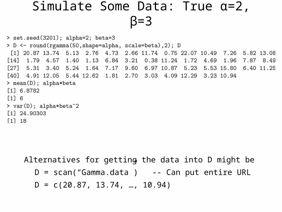
Simulate Some Data: True α=2, β=3

Alternatives for getting the data into D might be

D = scan(“Gamma.data”) -- Can put entire URL

D = c(20.87, 13.74, …, 10.94)

Log Likelihood

R function for the minus log likelihood

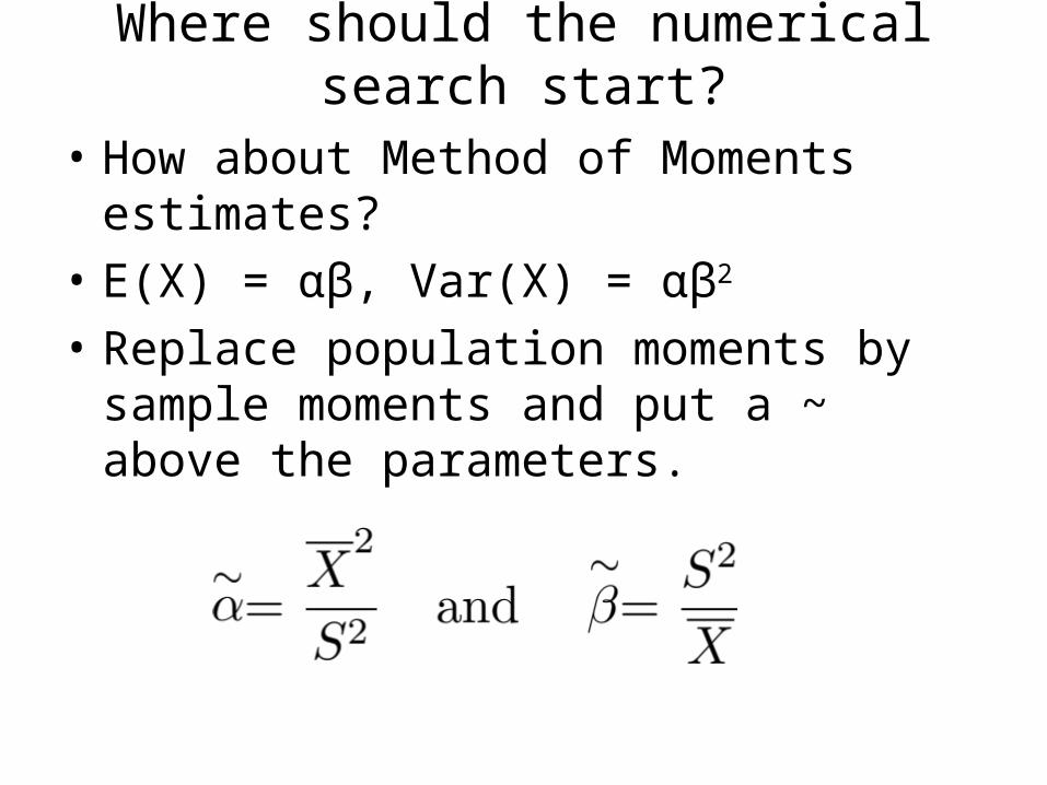
Where should the numerical search start?

• How about Method of Moments estimates?

• E(X) = αβ, Var(X) = αβ2

• Replace population moments by sample moments and put a ~ above the parameters.

If the second derivatives are continuous, H is symmetric.

If the gradient is zero at a point and |H|≠0, If H is positive definite, local minimum

If H is negative definite, local maximum

If H has both positive and negative eigenvalues, saddle point

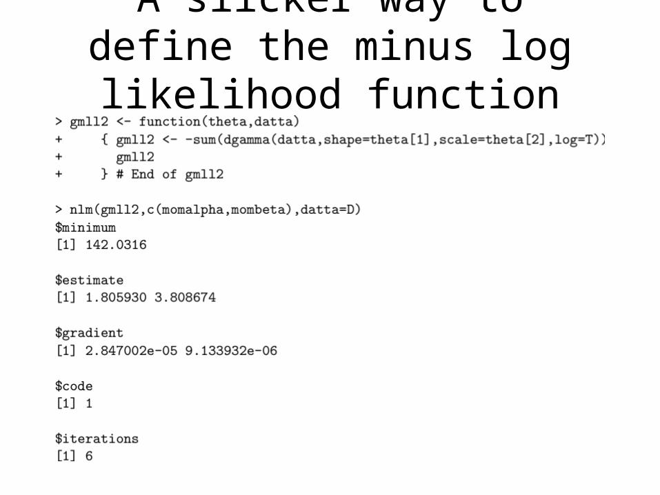
A slicker way to define the minus log likelihood function

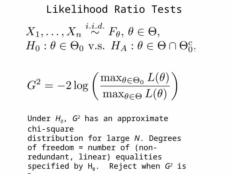
Likelihood Ratio Tests

Under H0, G2 has an approximate chi-square distribution for large N. Degrees of freedom = number of (non-redundant, linear) equalities specified by H0. Reject when G2 is large.

Example: Multinomial with 3 categories

• Parameter space is 2-dimensional

• Unrestricted MLE is (P1, P2): Sample proportions.

• H0: θ1 = 2θ2

Parameter space and restricted parameter space

R code for the record

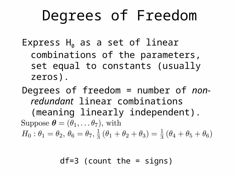
Degrees of Freedom

Express H0 as a set of linear combinations of the parameters, set equal to constants (usually zeros).

Degrees of freedom = number of non-redundant linear combinations (meaning linearly independent).

df=3 (count the = signs)

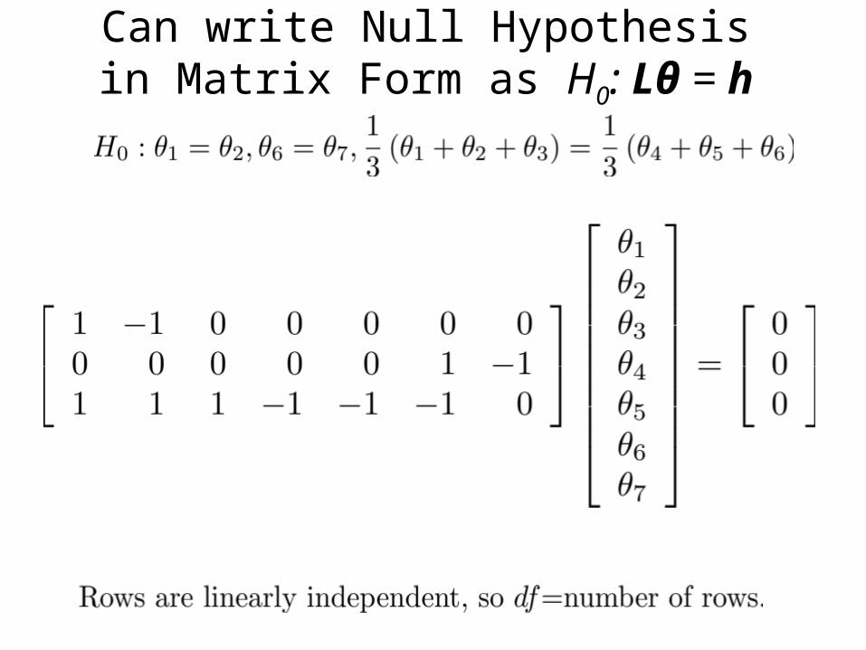
Can write Null Hypothesis in Matrix Form as H0: Lθ = h

Gamma Example: H0: α = β

Make a wrapper function

It's probably okay, but plot -LL

Test H0: α = β

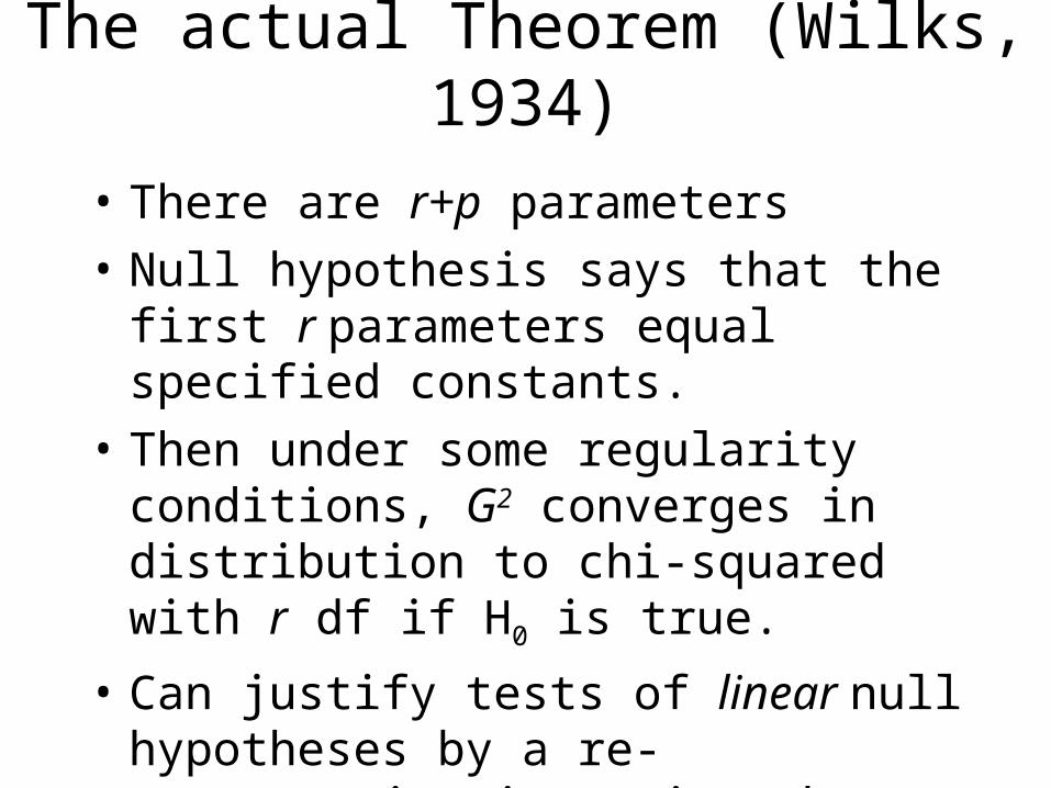
The actual Theorem (Wilks, 1934)

• There are r+p parameters

• Null hypothesis says that the first r parameters equal specified constants.

• Then under some regularity conditions, G2 converges in distribution to chi-squared with r df if H0 is true.

• Can justify tests of linear null hypotheses by a re-parameterization using the invariance principle.

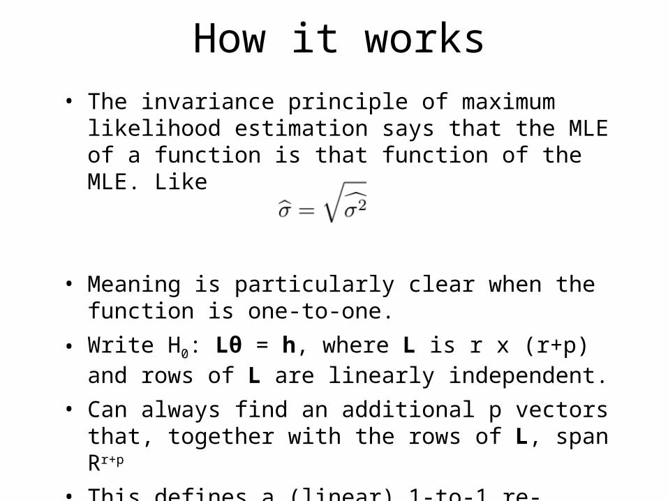
How it works• The invariance principle of maximum likelihood

estimation says that the MLE of a function is that function of the MLE. Like

• Meaning is particularly clear when the function is one-to-one.

• Write H0: Lθ = h, where L is r x (r+p) and rows of L are linearly independent.

• Can always find an additional p vectors that, together with the rows of L, span Rr+p

• This defines a (linear) 1-to-1 re-parameterization, and Wilks' theorem applies directly.

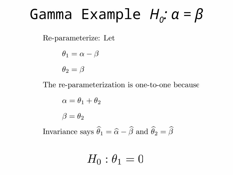
Gamma Example H0: α = β

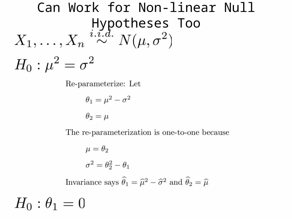
Can Work for Non-linear Null Hypotheses Too

Copyright Information

This slide show was prepared by Jerry Brunner, Department of

Statistics, University of Toronto. It is licensed under a Creative

Commons Attribution - ShareAlike 3.0 Unported License. Use

any part of it as you like and share the result freely. These

Powerpoint slides will be available from the course website:

http://www.utstat.toronto.edu/~brunner/oldclass/appliedf14