JOURNAL OF MULTIVARIATE ANALYSIS 12, 256-269 (1982)

Maximizing the Probability of Correctly Ordering Random Variables Using Linear Predictors

STEPHEN Po~mou*

Department of Mathematics, University of Illinois, Urbana, Illinois 61801

Communicated by S. Das Gupta

Let CT,, x,), CT,, x2),..., CT,, XJ b e a sample from a multivariate normal distribution where r, are (unobservable) random variables and x, are random vectors in Rk. If the sample is either independent and identically distributed or satisfies a multivariate components of variance model, then the probability of correctly ordering {T,) is maximized by ranking according to the order of the best linear predictors (E(T,Ix,)}. Furthermore, it orderings are chosen according to linear functions {b’x,] then the conditional probability of correct order given (T, = t,; i = l,,.., n) is maximized when b’x, is the best linear predictor. Examples are given to show that linear predictors may not be optimal and that using a linear combination other than the best linear predictor may give a greater probability of correctly ordering (r,} if ((T,, xt)) are independent but not identically distributed, or if the distributions are not normal.

1. INTR~DLJcTI~N

In many situations, an experimenter wishes to make inferences on an unobservable random vector, T = (T,, T,,..., T’,)‘, on the basis of an obser- vable vector X. We introduce the multivariate normal model,

where the mean and covariance structure are assumed known. Searle [6] considered primarily the problem of predicting T, on the basis of a linear combination of co-ordinates of X. Here we are concerned with the problem of ordering or ranking the {Ti} on the basis of functions of the co-ordinates of X. In Henderson [4] and Searle [6], it is shown that (under appropriate conditions) the probability of correct pairwise order is maximized by

Received December 5, 1979; revised February 6, 1981. AMS 1980 subject classification: Primary 62105. Key words and phrases: Linear predictors, selection index, multivariate normal. * This work was facilitated by National Science Foundation Grants MCS-78-04014, MCS-

79-0258 1, and MCS-80-02340.

256 0047.259X/82/020256-14$02.00/0 Copyright 0 1982 by Academic Press. Inc.

CORE Metadata, citation and similar papers at core.ac.uk

Provided by Elsevier - Publisher Connector

ORDERING RANDOM VARIABLES 257

ordering a pair (T,, T,) according to the best linear predictors (based on X.) An alternate shorter proof is given in Section 2 (Corollary 2.2). Furthermore, the following results are presented.

(1) Suppose for each i = l,..., n there are co-ordinates of X, say, x,, such that (T, , xl), (T,, x2),..., (T,, x,) are either independent and identically distributed (equivalently, V, C, and P are block diagonal with the diagonal blocks all identical) or obey the components of variance structure described in (4.1). Then the probability of correctly ordering { ri} is maximized by ranking according to the order of the best linear predictors. Furthermore, for every (ti ,..., tJ, the conditional probability given {Ti = f, ; i = l,..., n} of correctly ordering {T,} by ordering according to the ranking of {b’x,} is maximized when b = P;‘c,, where P, and c, are the ith blocks of P and C, respectively (which is equivalent to using the best linear predictors).

(2) It is shown by examples that in the general case (l.l), procedures other than ranking according to the best linear predictors can give strictly larger probability of correctly ordering {T,}. In fact, one example is of the form in (1) with (T,, xi) independent but not identically distributed; and ordering according to the best linear predictor actually has smaller probability than choosing an ordering at random. Another example is given to show that the normality assumption cannot be substantially generalized.

This problem was suggested in the context of animal breeding applications (e.g., see Hazel [3] or Henderson [5]). H ere Ti is a linear combination of (unobservable) genetic variables weighted by economic factors; and it is desired to find the largest values for T, on the basis of linear combinations I, = b; X, where Z is referred to as a selection index and X is a vector of measurements of phenotypic variables. However, as Searle [6] noted there is a wide variety of ranking and selection problems where model (1.1) is appropriate. If correct ranking is of crucial importance then the examples of Section 5 show that use of the best linear predictors may be inappropriate if the sampling situation does not obey the models of Sections 3 and 4. Theorem 2.1 describes how to find the best ordering in the general case by examining all n! possibilities. It would be useful and interesting to find a simpler algorithm which would identify the best ordering when n is not small enough to make it computationally feasible to compute n! multivariate normal probabilities in R”.

Remarks. (1) It is straightforward to extend the results of this paper to other selection problems. For example, the theorems of Sections 2, 3, and 4 can be extended to the problem of selecting N co-ordinates containing the k largest Ti values by simply replacing the cone Ci (i = l,..., n!), giving a specific ordering of the co-ordinates, by the cone Di (j = l,..., (l)), giving a specific subset of N co-ordinates containing the k largest ones. The coun- terexamples of Section 5 also hold for such selection problems.

258 STEPHEN PORTNOY

(2) Eaton [2] obtained general decision theoretic results (admissibility and minimaxity) when T is considered an unknown parameter. His results also hold in the independent case or when there is one other component of variance, but not more generally.

2. MAXIMIZING THE PROBABILITY OF CORRECT ORDER

For the basic theorem let T E R” and X E R” be random vectors with an arbitrary joint density in R”+m. For i = l,..., n! let Ci c R” denote the set of vectors in R” whose co-ordinates have the ith strict ordering; e.g., C, =

((X I,...) x,): x1 < xz < * * * < x,}. Define “the Ci ordering” to be the ordering of co-ordinates for vectors in Ci.

THEOREM 2.1. Under the above assumptions, the rule based on values of x E R”’ maximizing the probability of correctly ordering the co-ordinates of T is th,e foIlowing: for each x choose that ordering Ci which maximizes P{T E C, 1 X = x} over i = I,..., n!.

ProoJ Consider the statistical decision problem with observation space = R”, parameter space = R”, and distributions given by the conditional density of X given T = t (for t E R “). Define the action space to be ~2 = { Ci : i = I,..., n! } and introduce the loss function L(A, t) = 0 if t E A and 1 if t 6$ A (for A E A?). Then for any decision rule, 4: Rm + -M’, the conditional probability of correct order given T = t is just one minus the risk of ql; and the unconditional probability is just the Bayes risk for the prior distribution given by the marginal distribution of T. Thus, the rule maximizing the probability of correct order is the Bayes rule with respect to the marginal distribution of T: for each x E Rm choose Ci E ~4 minimizing E[L(Ci, T) ( X =x1. Clearly, this conditional loss is minimized by choosing Ci so that L(C,, T) = 0 with greatest conditional probability; that is, by choosing Ci to maximize P{T E Ci ] X = x). 1

Under model (1. I), the conditional distribution is multivariate normal with mean E[T ] X = x] linear in x and covariance matrix independent of x (note that E[T ] X = x] is the best predictor of T given X = x). Thus, the general problem is reduced to finding that Ci with maximum probability under a given multivariate normal distribution. In certain general cases, the best rule is to choose that C, containing E [T ] X = x] (that is, order co-ordinates of T according to the order of the best predictor). However, as Example 5.1 shows, the best rule is not based on E[T ] X = x] in general.

COROLLARY 2.2. Under model (l.l), $ n = 2 (that is, only two unob- served variables are to be compared) the probability of correct or&r is

ORDERING RANDOM VARIABLES 259

maximized by ranking according to the order of E [Tj ] X = x] (j = 1,2). If the means satisfy p, = Pz and v = 0 then the ranking depends on a linear function of x whose coeflcients depend on the covariance structure but not the means.

Proof In this case, C, and Cr are half spaces with common boundary equal to the main diagonal of R 2. Geometrically, any bivariate normal distribution is constant on ellipses; and the half space containing the center of the ellipse will contain the greatest fraction of the ellipse. The corollary follows since the center of each ellipse is the conditional mean, E[T 1 X = x]; and (if v = 0) E[T, ] X = x] = pt + bf x, where b, is a vector of coefficients depending only on the covariance. If pi = p,, the order depends only on bfx. 1

If n > 2 there are some simple general facts about when the ordering, C,, containing E[T 1 X = x] is best. Clearly, if P(C, )X =x) > 0.5 then C, maximizes the probability of correct order. (This follows since the boundary of two orderings has zero probability; and, hence, there can not be a second ordering with probability greater than 0.5.) On the other hand, if C, # C*, where C* maximizes P(C, ] X =x) (over i = l,..., n!), then P(C* ] X = x) < 0.5. This follows from Corollary 2.2 as follows: let S be a half space such that C* c S but E[T ] X = x] & S. Then (by the proof of Corollary 2.2) P(S ] X = x) Q P(Sc ] X = x) = 1 - P(S ) X = x); whence, P(c*(x= x) Q P(S ] X=x) Q 0.5. Thus, if C, is not optimal, the best ordering C* cannot be too good. However, even if C, is optimal, it may have small conditional probability (if n > 2).

In general, the examples of Section 5 show that strong conditions are needed to show tht C, is optimal. The following condition seems nearly as weak as possible.

THEOREM 2.3. Under model (ll), suppose that the conditional covariance matrix of T given X = x is an interclass correlation matrix. That is,

Cov(T ( X = x) = a1 + pee’, (2-l)

where e= (1 1 .a. 1)‘. Also assume p = ne (j?rr some constant n) and v = 0. Then the probability of correctly ordering the co-ordinates of T is maximized by choosing the ordering, C,, such that E[T ) X = x] E C, (i.e., by ranking according to the order of the best linear predictor); and furthermore the ranking does not depend on n.

Proof. Let n(i, j) denote the n x n permutation matrix interchanging co- ordinates T1 and TJ (and not changing any other co-ordinates). Let u1 =

260 STEPHEN PORTNOY

E[T, ) x = x ] (i = l,..., n). It will first be shown that if C, is an order such that ui > ui for u E C, then

P{TEC,IX=x}>P{TEIr(i,j)C,IX=x}. P-2)

To do this, condition further on { 7’,} for I # i and 1# j. Consider the case where C, is such that, for T E C,, Ti and Tj are neither the smallest nor the largest co-ordinate, nor are they adjacent in order (other cases will follow similarly). Then given (T!} for 1# i ori let A k be the value of the co-ordinate preceding Ti (in order C,), B 1 that succeeding Ti, A z that preceding Tj, and B, that succeeding Tj. It follows that there are (random) sets S, and S, depending on A ,, A,, B,, and B, in RZ (see Fig. 1) such that

P{TECk(X=x}=EP{ZES,},

P{TEn(i,j)C,IX=x)=EP(ZES2}, (2.3)

where Z = (Tj, Ti) and has the conditional distribution given X = x and T, = t, (for 1 f i or j), and expectation is over the conditional distribution of A,, B,, A,, 8, given X=x over C,. If (2.1) holds, direct computations show that the mean of 2, and covariance matrix of Z (conditional on X = x and T,= f, for If i orj) are

EZi = Ui + rZ C (T, - u,), 1zi.j

Cov(Z) = cd + /lAee’, (2.4)

FIG. 1. Projection into T,T, plane.

ORDERING RANDOM VARIABLES 261

where A =/3/(a + (n - 2)p). That is, if Ui > nj, EZ, > EZ,; and the conditional covariance matrix has one principal axis parallel to the main diagonal and the other perpendicular to it (see Fig. 1). To compute (2.3), first integrate along lines L, c S, and L, c S, perpendicular to the main diagonal (see Fig. 1); that is, condition on Z, + Z, = z and compute P{Z, -Z, EL, ) z} for v = 1,2). Since EZ, > EZ,, P{Z, -Z, EL, 1 z) > P{Z, - Z, E L, ) z}. Integrating z between a and b (in Fig. l), it follows that P{Z E S,} > P{Z E S,} (independent of the values of A,, A,, B,, and B2). Therefore, (2.2) follows by taking expectations over (T,} (I # i, j) using (2.3).

Now for any C, and given C, it is possible to find a finite product of transpositions x1 . . . x, (each factor being n(i, j) for some (i, j)) such that C,=n, .** n,C,. Thus, applying (2.2) inductively (using the fact that E[T 1 X = x] E C, at each step), proves the theorem. 1

3. THE i.i.d. CASE

Let CT,, x1), (T,, x2),..., (T,, xn) be an independent and identically distributed (i.i.d.) sample from a multivariate normal distribution in (k + 1) dimensions. Then the conditional distribution of T given X = x has i.i.d. co- ordinates; and, hence, (2.1) holds (with /I = 0 and q the common mean). Therefore, Theorem 2.3 immediately yields:

THEOREM 3.1. In the i.i.d. case described above, the probability of correctly ordering co-ordinates (T,,..., T,,) is maximized by ranking according to the order of the best linear predictors {E[ Ti 1 Xi = Xi]: i = l,..., n}, and the ranking does not depend on the means of (Ti, xi).

If one restricts attention to orderings based on linear predictors, the best linear predictors, E(T, 1 X = x), have the uniform optimality property of maximizing the conditional probability of correct order given T = t (for any t E RR). To see this, make the definitions

JW’J = A Var(T,) = u’,

and

E(q) = 0, Cov(x,) = P, COV(Ti, Xi) = C.

Then for any bE Rk

(3.1)

(3.2)

Hb’x, I T,l p@Fii =!$(Ti-P)= o, (T,-P),

(3.3) Var [b’x, 1 T,] = (b’Pb)(l - p’),

262 STEPHEN PORTNOY

where

(b’c)2 ‘* = a;(b’Pb) *

For any b E Rk introduce the normalization

bN = b/&i%,

(3.4)

(3.5)

and note that p (in (3.4)) is the same for b and b,. The following definition is also needed: a Conrad cone, C c R”, is a set

such that the origin 0 E C and if x, y E C and u 2 0, x + uy E C also. Note that Ci is a convex cone, and for any continuous distribution P(CJ = P(C,).

THEOREM 3.2. Consider the sampling sihtation given above. Let T E R” and X(n X k) denote

T’ = (T, ,..., T,); X’ = (x, y.:, x,). (3.6)

Let b* = P - ‘c (so that Xb * is the best predictor of T). Then for any b E R k t E R” and any convex cone C c R ‘,

P(Xb*EC,T-peEC)T=t}>P{XbEC,T-peEC(T=t}.

In particular, the inequality holds for orderings Cr (for which T E Ci if and only if T -pe E Ci).

In a personal communication Professor Shanti Gupta showed that the proof could be simplified somewhat if arbitrary cones are not considered. However, the basic ideas are the same and the additional generality seems desirable. Thus to prove the theorem the following lemma concerning probability content of convex cones is needed:

LEMMA. Let C c R” be a convex cone and let v E C, o > 0, a > 1, and d < 1. Let Z and Y be two random vectors in R” with (Z - V)/U - (Y - dv)/(aa) (that is, they have the same distribution, say, Q). Then

P{Y E C} < P{Z E C).

Proof of Lemma. Define A = {x: aox + dv E C} and B = {x: ox + v E C}. Then (since C is a convex cone)

ORDERING RANDOM VARIABLES 263

xEA=>uox+dvEC ~aox+dv+(a-d)vEC *aax+avE c =z- 0 + (l/u)(uox + uv) E c

*ux+vEC

*xEB.

Therefore, A c B; and hence (with Q as before)

P{YEC}=P s&4 1 I

= Q(A)< Q(B)=P /yEB/ =P{ZEC}. I

Proof of Theorem 3.2. Let b be an arbitrary vector in Rk and (as above) b* =P-‘c. Let e = (1 1 ... 1)’ E R”. Then from (3.3), (3.4), and normalization (3.9,

EP% I Tl =$-(T-pe)=c(T-pe),

52 = 1 -l!!!q 14 Cov[Xb, 1 T] = t*I, UT

(3.7)

Therefore the following vectors have the same (unit multivariate normal) conditional distribution given T,

z= Xb,* --p*(T -,ue)/u,

&qF ’

y = Xb,-Pp -lue)bJT j/m ’

where p and p* are defined by (3.4) using b and b*, respectively. Now it is well known that b * maximizes the correlation between Ti and b’xi ; so p* > p. Thus, the lemma can be applied with u2 = 1 - p* 2, v = p *(T - pe)/u,, d = p/p* < 1, and a = d-/d- > 1. Therefore, for any convex cone C c R” containing T -pe,

P{Xb,*ECIT}>P{Xb,ECIT),

and the theorem follows. m

(3.8)

264 STEPHEN PORTNOY

4. THE MULTIVARIATE COMPONENTS OF VARIANCE STRUCTURE

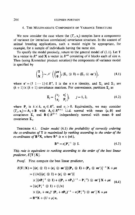
We now consider the case where the (Ti, xi) samples have a components of variance (or intraclass correlation) covariance structure. In the context of animal breeding applications, such a model might be appropriate, for example, for a sample of individuals having the same sire.

To specify the model precisely, return to the general model of (1.1). Let T be a vector in R” and X a vector in Rnk consisting of k blocks each of size n. Then (using Kronecker product notation) the components of variance model is specified by

G)-x ((“o’)v (zl 0 1) + (I;, 0 ee’)

i , (4-l)

where e’ = (1 1 -.a 1) E R”, I is the n X n identity, and Z, and & are (k+ 1)x (k+ 1) covariance matrices. For convenience, partition Zj as

x, = ‘j ‘i’

( ) cj P, ’ j= 1,2, (4.2)

where Pj is kx k, cjE Rk, and uj > 0. Equivalently, we may consider (Ti,xi)=Ai+B with AiERk” i.i.d. normal with mean (,u, 0) and covariance ?Z, and B E Rk+ ’ independently normal with mean 0 and covariance Zz.

THEOREM 4.1. Under model (4.1) the probability of correctly ordering the co-ordinates of T is maximized by ranking according to the order of the co-ordinates of B*X, where B* is n x (nk),

B* =c;P;’ @ I. (4.3)

This rule is equivalent to ranking according to the order of the best linear predictor, E[T 1 X].

ProoJ First compute the best linear predictor,

E(T 1 X) = [(cl 0 I) + (c; 0 ee’)][(P, 0 I) + (Pz 0 ee’)]-’ X +pe

= (l/n)[(cl 0 I) + (c; 0 =‘)I

x[(nP;’ 0 I)+((P,+nP,)-I-P;‘) 0 ee’]X+,ue (44)

= [(clP;’ 0 I) + (l/n)

X ((cl + ncJ (P, + nP,)-’ - c;P;‘) 0 ee’] X +pe

=B*X + (U+p)e,

ORDERINGRANDOMVARIABLES 265

where U is a constant linear function of X. Thus, the co-ordinates of the best linear predictor are ordered as B*X.

Now, to apply Theorem 2.3, Cov[T ] X] is computed. If A denotes the coefficients of B[T ] X], then, from (4.4),

Cov[T ] X] = Cov(T) - A[(c, @ I) + (c, @ ee’)]

=u, @ I+u, @ ee’-c;P;‘c, @ I-(l/n)a @ ee’,

where rfj are given in (4.2) and

a = (c, + nc,)’ (P, + nP,)-’ (c, + nc*) -c;p;‘c,.

Since the first factor in each Kronecker product is a scalar, Cov[T ] X] is an intraclass correlation matrix (and so satisfies (2.1)). Thus, Theorem 2.3 holds and the probability of correct order is maximized by choosing Ci such that E[T ] X] E C,. Thus, the theorem follows from (4.4). 1

To maximize the conditional probability of correct order given T = t, restrict consideration to “stationary” linear predictors BX (where B is n x (nk)) of the form

B = (b; @ I) + (b; @ ee’), (4.5)

where b, and b, lie in Rk.

THEOREM 4.2. Under model (4.1), the conditional probability, given T = t, that the order of the co-ordinates oft is the same as the order of the co-ordinates of BX is maximized over B, satisfying (4.5) by B = B *, with B * given by (4.3).

Note that if B does not satisfy (4.5), the conditional probability of correctly matching the order of T, given T = t, can be made quite large for each specific value of t; that is, given the order of T, the probability of matching it can clearly be improved. Thus the strongest (conditional) form of optimality could not hold for B*.

Proof of Theorem 4.2. Let r be an n x n orthogonal matrix with first row e’/fi and let r, denote the last (n - 1) rows of r. Then

(Ior) ; ( 1

-N(v, (I;, 0 I) + n(& 0 J)),

where v has first element fip and all others zero and J is n X n with the (1, 1) element unity and all other entries zero. Therefore,

266 STEPHEN PORTNOY

and the blocks of Y have exactly the same distribution as given by (3.1) and (3.2).

Now, as before, let Ci (i = l,..., n!) be the convex cone of the ith ordering of co-ordinates in R”. Let y E R” and note that since the main diagonal of R” is in the boundary of Ci for all i, y E Ci if and only if I1 y E Ii Ci (since membership in Ki will be determined by the co-ordinates (I, Ci) orthogonal to the first co-ordinate). Thus, for B given by (4.5).

BXECioI,B(I 0 I’)(I @ I’)XEI,Ci

o((l/n)b, 0 I)YEI,Ci.

Therefore,

P(BXEC,fT}=P{((l,‘n)b, @ I)YEr,CiIT}. (4.7)

But Theorem 3.2 can be directly applied to the model given by (4.6) in R”- ‘. Thus, it follows that the probability in (4.7) (which is independent of b,) is maximized (for all i) at b f = P - ‘c. Since b, is arbitrary, we may choose bf = 0. This proves Theorem 4.2. As in Theorem 4.1 this rule is equivalent to ordering according to the co-ordinates of the best linear predictor. m

5. COUNTEREXAMPLES IN MORE GENERAL CASES

EXAMPLE 5.1. Under model (1.1) suppose that T and X are three dimen- sional with zero means. Let T and X be the projections into the plane orthogonal to the main diagonal of R3. Denoting this plane as the x-y plane, the orderings C, (i = l,..., 6) are projected into the cones indicated in Fig. 2. In particular, the following projection is being used: for z E R3,

x = (2, - 22, + z3) 6,

Y = t-1 + z,>/fl.

For each E > 0 define the covariance structure of (X, T) so that X is concen- trated near the y-axis (i.e., the variance of the x co-ordinate is E’) and such that the variance of the y co-ordinate of X is e. Given X let T be such that E[T ] X] = X and the conditional covariance matrix of T given X is concen- trated very near a line (through X) parallel to the x-axis (i.e., the variance of the y co-ordinate is a’) and is such that the conditional variance of the x co- ordinate of T (given X) is nearly 1 (see Fig. 2). Then, arguing geometrically from Fig. 2, E[T ] X] E C, U C, with probability tending to 1 as E + 0, but conditional on X, f E C, U C, U C, U C, with probability tending to 1. Therefore as E + 0, the probability that T has the same order as E[T 1 X]

ORDERING RANDOM VARIABLES 267

FIG. 2. Projection into x-y plane orthogonal to main diagonal.

tends to 0 (as E + 0); and, hence, the conditional probability given T also converges to 0. However, the probability of correctly ordering T using the best rule (from Theorem 2.1) tends to 4 as E + 0 ( and the conditional probability given T = t is positive for all t).

This example can be transformed back to yield the covariance structure (using the notation of (1.1))

v= i

1 0 l--E 0 2E 0

l-&O 1

Direct calculations using (5.1) can verify the conclusions inferred geometrically above.

EXAMPLE 2. A similar, though not as strong, example can be obtained even when samples (T,, XJ are independent but not identically distributed. Again let T and X be three dimensional with zero means, and using the notation of (1.1 ), let

V=(; i ;), C=(; ~1 i), P=I. (5.2)

268 STEPHEN PORTNOY

Then E[TIX]=C’P-‘X=CX=(EX,,E%~,E’X~). (5. 3)

First consider the (marginal) probability of each ordering of co-ordinates of T. Direct computations yield (as E + 0)

P{T, < T, < T3}=P{TI < T, < 7’2}+,

P{T,<T,<T,}=P{T,<T,<T,}-tt, (5.4)

P{T, < T,< T,}=P(T3 < T,< T,}-+$.

Now note that Corr(T,, X,) = c*, Corr(T,, X,) = s3, and Corr(T,, Xi) = s/fi =&. Thus, as E -+ 0, T and X tend to become independent; and to find the limiting probability of matching order, only marginal probabilities need to be computed.

For the probabilities of orderings of CX = (&XI, szX,, e3Xj), direct computations yield (as E -+ 0)

limP{aZX2 < sX, < s3X3} =limP{s3X3 < eX, <&*X2} =O,

but all other orderings have probabilities tending to i. Thus the probability that the order of T matches the order of CX is

i P(TEC,,CXECJ+, .$+~.++$.o+$.o++~+Q.a i=l

1 =y.

However, each ordering of X itself is equally likely (since Cov(X) = I). So the probability that the order of T matches the order of X tends to d; and, thus, for E small enough X is better in terms of the probability of matching order than the best linear predictor CX. It is interesting to note that X is better than CX even if we only wish to match maxima. Again direct computations show that as E + 0 the probability that the index of max(T,, T2, T,) equals the index of max(X,, X2, X,) tends to 4 ; but the probability that it equals the index of max(&X, , s*X,, s3X3) tends to 5/16.

Note also that a model like (4.1) with three or more components of variance could be reduced by means of an orthogonal transformation to the covariance structure in (5.2). Thus, Example 2 shows that the optimality results of the earlier sections could not hold in such more general cases.

EXAMPLE 3. It is possible to extend some of the results to cases where the distributions are not multivariate normal. In particular, Theorem 2.1 is already stated more generally, and Theorems 3.2 and 4.2 depend only on computations involving conditional means and covariance matrices. Thus, if

ORDERING RANDOM VARIABLES 269

conditional means are linear, conditional covariances are constant, and conditional distributions form multivariate location-scale families, the results of Theorems 3.2 and 4.2, still hold. But these restrictions are very serious: for example, if conditional means are not linear, the best linear predictor may be of little value.

To obtain a specific example, let Xi N X(0, 1) for i = 1,2 and let Ti = X: - 1 + LX, (i = 1,2). Then EXi Ti = E and the best linear predictor is (&X1, LX*). As above, as E -P 0 it is easy to show that

But Ti is a function of X,; so using the predictor with co-ordinates Xt- 1 +Exi,

ACKNOWLEDGMENTS

The author wishes to thank Professor D. Gianola of the Department of Animal Sciences for suggesting the problem and making some helpful comments, and wishes to thank the referee for his careful reading and important suggestions.

REFERENCES

[ 1] COCHRAN, W. G. (1951). Improving by means of selection. In Proceedings, Second Berkeley Symposium, p. 449.

[2] EATON, M. L. (1967). Some optimum properties of ranking procedures. Ann. Math. Statist. 38, 124.

[3] HAZEL, L. N. (1943). The genetic basis for constructing selection indexes. Genetics 28, 476.

(41 HENDERSON, C. R. (1963). Selection Index and Expected Genetic Advance. NAS-NCR 982.

[S] HENDERSON, C. R. (1973). Sire evaluation and genetic trends. In Proceedings, Animal Breeding and Genetics Symposium in Honor of J. L. Lush, p. 10. Amer. Sot. Anim. Sci., Champaign, Ill.

[ 61 SERLE, S. R. (1974). Prediction, mixed models, and variance components. In Proceedings, Conference on Reliability and Biometry (Proschan and Serfling, Eds,), p. 229. SIAM, Philadelphia.