Maximizing Queueing Network Utility Subject to Stability ...
57
Queueing Systems 50, 401–457, 2005 c 2005 Springer Science + Business Media, Inc. Manufactured in The Netherlands. Maximizing Queueing Network Utility Subject to Stability: Greedy Primal-Dual Algorithm ALEXANDER L. STOLYAR [email protected] Bell Labs, Lucent Technologies, 600 Mountain Ave., 2C-322, Murray Hill, NJ 07974, USA Received 4 August 2004; Revised 4 February 2005 Abstract. We study a model of controlled queueing network, which operates and makes control decisions in discrete time. An underlying random network mode determines the set of available controls in each time slot. Each control decision “produces” a certain vector of “commodities”; it also has associated “traditional” queueing control effect, i.e., it determines traffic (customer) arrival rates, service rates at the nodes, and random routing of processed customers among the nodes. The problem is to find a dynamic control strategy which maximizes a concave utility function H ( X ), where X is the average value of commodity vector, subject to the constraint that network queues remain stable. We introduce a dynamic control algorithm, which we call Greedy Primal-Dual (GPD) algorithm, and prove its asymptotic optimality. We show that our network model and GPD algorithm accommodate a wide range of applications. As one example, we consider the problem of congestion control of networks where both traffic sources and network processing nodes may be randomly time-varying and interdependent. We also discuss a variety of resource allocation problems in wireless networks, which in particular involve average power consumption constraints and/or optimization, as well as traffic rate constraints. Keywords: queueing networks, convex optimization, primal-dual algorithm, stability, congestion control, resource allocation, scheduling, wireless, power and rate constraints AMS subject classification: 90B15, 90C25, 60K25, 68M12 1. Introduction 1.1. The problem We study a model of controlled queueing network, which operates and makes control decisions in discrete time t = 0, 1, 2,... . The key feature of the model is that each network control action has two effects. First, network has a finite set N p of “traffic” processing nodes, with queues, and each control action has associated “queueing con- trol” which affects traffic (customer) arrival rates to processing nodes, their processing (service) rates, routing between processing nodes, etc. Second, network generates a fi- nite number of “commodity (utility) flows,” forming set N u ; namely, each control action k generates amounts b n (k ), n ∈ N u , of the commodities. In addition, the available set of control options depends on some underlying random network “mode,” modelled by an ergodic Markov chain.
Transcript of Maximizing Queueing Network Utility Subject to Stability ...
Queueing Systems 50, 401–457, 2005c© 2005 Springer Science + Business Media, Inc. Manufactured in The Netherlands.
Maximizing Queueing Network Utility Subjectto Stability: Greedy Primal-Dual Algorithm
ALEXANDER L. STOLYAR [email protected] Labs, Lucent Technologies, 600 Mountain Ave., 2C-322, Murray Hill, NJ 07974, USA
Received 4 August 2004; Revised 4 February 2005
Abstract. We study a model of controlled queueing network, which operates and makes control decisionsin discrete time. An underlying random network mode determines the set of available controls in each timeslot. Each control decision “produces” a certain vector of “commodities”; it also has associated “traditional”queueing control effect, i.e., it determines traffic (customer) arrival rates, service rates at the nodes, andrandom routing of processed customers among the nodes. The problem is to find a dynamic control strategywhich maximizes a concave utility function H (X ), where X is the average value of commodity vector,subject to the constraint that network queues remain stable.
We introduce a dynamic control algorithm, which we call Greedy Primal-Dual (GPD) algorithm, andprove its asymptotic optimality. We show that our network model and GPD algorithm accommodate a widerange of applications. As one example, we consider the problem of congestion control of networks whereboth traffic sources and network processing nodes may be randomly time-varying and interdependent. Wealso discuss a variety of resource allocation problems in wireless networks, which in particular involveaverage power consumption constraints and/or optimization, as well as traffic rate constraints.
Keywords: queueing networks, convex optimization, primal-dual algorithm, stability, congestion control,resource allocation, scheduling, wireless, power and rate constraints
AMS subject classification: 90B15, 90C25, 60K25, 68M12
1. Introduction
1.1. The problem
We study a model of controlled queueing network, which operates and makes controldecisions in discrete time t = 0, 1, 2, . . . . The key feature of the model is that eachnetwork control action has two effects. First, network has a finite set N p of “traffic”processing nodes, with queues, and each control action has associated “queueing con-trol” which affects traffic (customer) arrival rates to processing nodes, their processing(service) rates, routing between processing nodes, etc. Second, network generates a fi-nite number of “commodity (utility) flows,” forming setN u; namely, each control actionk generates amounts bn(k), n ∈ N u , of the commodities. In addition, the available setof control options depends on some underlying random network “mode,” modelled byan ergodic Markov chain.
402 STOLYAR
Let X = (Xn, n ∈ N u), be the vector of long-term average rates at which com-modities are generated under a given control strategy. We seek to find a dynamic controlstrategy which maximizes a concave utility function H (X ) of average commodity rates,subject to the constraint that the network remains stable, that is, roughly speaking, queuesat the processing nodes remain bounded. (The utility function H need not be strictlyconcave.) In this paper we introduce a dynamic control algorithm, called Greedy Primal-Dual (GPD) algorithm, which solves the above problem (asymptotically, as describedshortly), under the natural assumption that, roughly speaking, it is feasible at all to keepthe network stable (even if we ignore utility optimization). As we will see, the algorithmis very parsimonious, and naturally decomposes to become a decentralized algorithm inspecial cases when different network elements can make “their own” control decisionsindependently.
Since both commodity generation and queueing control actions depend on a cho-sen network control action, our model accommodates, in general, scenarios in which“currently available” choices of commodity generation rates, traffic arrival and servicerates, and routing are mutually interdependent in arbitrary way. As we will see, thisfeature is very useful in modelling many systems arising in applications.
In applications, different commodity types may have different meanings, and someof the commodities may be “physical” and some “virtual.” In telecommunication systemsa commodity may be a traffic flow, which may (or may not) need to go through and beprocessed by the processing network (this is modelled by “coupling” the generatedcommodity amounts and amounts of arrived traffic to some nodes). A commodity mayalso correspond to a monetary award (or penalty), associated with a control action. Or,going back to telecommunications, and in particular wireless systems, a commodity maybe energy or power consumed by a control action. Thus, a commodity may be virtualin the sense that it serves simply to keep track of and optimize certain performancemeasures. For example, the GPD algorithm can be used to control a queueing networkat the lowest average cost (or power consumption), while keeping queues stable. Someexamples of applications are discussed in Section 5. We will demonstrate there that theGPD algorithm can create virtual processing nodes as well; for example, to solve thestated optimization problem, subject to additional desired constraints on the averagecommodity generation rates. To summarize, our abstract view that network controlactions have double effect of controlling queues on one hand, and generating somecommodities on the other hand, allows the model to accommodate a large variety ofapplications and scenarios.
1.2. Informal description of the GPD algorithm
Formal definitions of the model and the GPD algorithm are given in Section 4. Here wedescribe the algorithm informally, to facilitate discussion.
Recall that bn(k), n ∈ N u , are the commodity amounts generated by control k.Denote by �Qn(k) the expected average (possibly negative) increment, or drift, of the
GREEDY PRIMAL-DUAL ALGORITHM 403
queue length Qn at a processing node n ∈ N p, caused by control k, assuming that allQn at all processing nodes were large enough for queues to not empty as a result of thecontrol. (Drift values �Qn(k) incorporate the aggregate effect of new arrivals, service,and inter-node routing associated with control k.) Assume that the utility function H iscontinuously differentiable. The GPD algorithm is such that, from all the control actionsk available at time t (with the set of available k depending on the underlying randomnetwork mode), it chooses a control
k(t) ∈ arg maxk
∑
n∈N u
(∂ H (X (t))/∂ Xn)bn(k) −∑
n∈N p
βQn(t)�Qn(k), (1)
where β > 0 is a (typically small) parameter, and X (t) is the vector of the “currentaverages” of commodity rates, updated as follows:
Xn(t + 1) = Xn(t) + β(bn(k(t)) − Xn(t)), n ∈ N u . (2)
Using natural vector notations, and “.” to denote scalar products, the GPD rule (1) canbe concisely written as follows:
k(t) ∈ arg maxk
∇ H (X (t)) · b(k) − βQ(t) · �Q(k). (3)
We prove asymptotic optimality of the GPD algorithm in the following sense:
(I) When parameter β is small, the rescaled trajectories (X (t/β), βQ(t/β)), t ≥ 0,under GPD algorithm, are close to trajectories (x(t), q(t)), t ≥ 0, of some dynamicsystem. (We call the latter GPD-trajectories.)
(II) If network structure and parameters are such that it is feasible at all to keep queuesstable, then, as t → ∞, all GPD-trajectories converge to points (v∗, q∗) suchthat H (v∗) is the maximum possible value of network utility under the stabilityconstraint.
Analysis of the dynamic system (in Section 3), including proof of the global uni-form attraction property of GPD-trajectories (Theorem 2), is in fact the key part of thispaper. The dynamic system is “primal-dual”—the attraction points (v∗, q∗) are optimalsolutions to some underlying convex optimization problem and its dual. To the bestof our knowledge, the dynamic system is not of any known primal-dual type. (Previ-ously studied primal-dual dynamic systems include, for example, the classical Arrow-Hurwicz-Uzawa system (cf. [13]) and systems within passivity framework of [26]).
1.3. Discussion
It is easy to observe that, if we remove all processing nodes from our model (so thatthere is no stability constraint), the GPD algorithm reduces to the Gradient algorithm [3,21], always “greedily” choosing controls maximizing the drift of utility (“Lyapunov”)function H (X (t)), and shown to be asymptotically optimal as β ↓ 0 in [3, 21]. If
404 STOLYAR
we remove all commodity flows (so that we are not concerned about any utility), theGPD algorithm becomes a “MaxWeight”-type algorithm (cf. [4,20,22,23]), “greedily”pursuing minimization of Lyapunov function
∑N p (1/2)Q2
n(t), and known to ensurestability of queueing networks if such is feasible at all. (Cf. [4] for recent results andreview of previous work.)
The GPD rule (3) shows that, roughly speaking, the algorithm always “greedily”chooses controls maximizing the expected drift of function
H (X (t)) −∑
n∈N p
(1/2)βQ2n(t),
and thus can be viewed as a “naive” combination of the Gradient and MaxWeight algo-rithms. The fact that such naive combination produces an algorithm which is (asymp-totically) optimal for our problem, is non-trivial and perhaps even surprising for thefollowing reasons. For a MaxWeight algorithm, function
∑(1/2)Q2
n(t) is in fact a Lya-punov function which ensures stability. For the Gradient algorithm, H (X (t)) is “almost”a Lyapunov function—it becomes such after X (t) gets close to a certain region (and con-vergence to the region is not very hard to establish [21]). In contrast, it is easy to see thatfor the GPD algorithm function H (X (t)) − ∑
(1/2)βQ2n(t) cannot serve as a Lyapunov
function ensuring convergence to an optimal point. (See discussion at the beginning ofSection 3.5.)
The proof of convergence is further complicated by the fact that we do not requireutility function H (X ) to be strictly concave. As a result, optimal points (attractors) v∗
may be non-unique. We avoid strict concavity assumption because it is too restrictive inmany applications of interest. Utility functions which are linear in some of the Xn arean obvious example.
Papers [20] and [21], which, in particular, study convergence properties of dynamicsystems arising as asymptotic limits under “pure MaxWeight” and “pure Gradient”policies, serve as starting points of our analysis.
Remark 1 (The role of parameter β). Note that, the scaling (X (t/β), βQ(t/β)), which inthe limit gives rise to GPD-trajectories (x(t), q(t)), is such that the space scaling by factorβ is applied only to queue lengths Q, but not to average rates X. Given (2), this ensuresthat both x(t) and q(t) change on the same scale in space. In the special case when thereis no utility nodes, the first term under the arg max in (3) vanishes, making parameterβ irrelevant, and leading (as already mentioned above) to MaxWeight algorithm, whichis known to be optimal for the purposes of network stability (and not using parameterβ). However, in the GPD algorithm (for the purposes of utility maximization subjectto stability), we cannot avoid using small parameter β in (1) and (2), roughly for thefollowing reason. For any algorithm to be “close to optimal,” a rule for choosing controlsk(t) must be “close” to the rule
k(t) ∈ arg maxk
∇ H (v∗) · b(k) − q∗ · �Q(k),
GREEDY PRIMAL-DUAL ALGORITHM 405
where v∗ and q∗ are optimal solutions to the underlying convex optimization problemand its dual. In order for βQ(t) to stay “close” to q∗ (and X (t) to be close to v∗),parameter β in (3) must be small. Then, Q(t) will be large (of the order of 1/β), and theincrements of βQ(t) small. Parameter β also determines the time scale on which X (t)and βQ(t) converge “close to” optimal values - the convergence time is of the order1/β. Thus, the smaller the β, the more “precise” the GPD algorithm is, but at the costof larger queue lengths and larger convergence times.
Remark 2 (More general form of GPD algorithm, with “weighted queue lengths”). Allour results still hold if the queue lengths Qn(t) in (3) are weighted by arbitrary constantsγn > 0. In other words, optimality of the GPD algorithm still holds if rule (3) is replacedwith the following more general one:
k(t) ∈ arg maxk
∇ H (X (t)) · b(k) −∑
n∈N p
βγn Qn(t)�Qn(k).
In this case the GPD-trajectories (x(t), q(t)) are such that x(t) still converges to optimalpoints v∗, but it is the weighted vector (γnqn(t), n ∈ N p), not q(t) itself, that convergesto an optimal point q∗. (See Section 3.8.2.) This is a useful property for applications.As discussed in Remark 1 above, when system is close to optimal operating point,the (unscaled) queue lengths Qn(t) are “large,” of the order 1/β. Introducing a weightγn > 1 for queue n will “scale down” a typical size of Qn(t) by factor γn . In other words,weights γn provide “knobs” allowing one to control queue length magnitudes. (But, ofcourse, using GPD algorithm with all large weights γn will reduce its “precision,” dueto reasons discussed in Remark 1.)
1.4. Applications
One application of our network model and the GPD algorithm, which we discuss insome detail in Sections 5.1 and 5.2, is to dynamic congestion control of communicationnetworks. Recent advances in the theory of network congestion control originate fromthe discovery [10] that the congestion control mechanism employed by the TransportControl Protocol (TCP) in the Internet implicitly attempts to maximize the sum of trafficflow (concave) utilities, subject to the constraint that none of the network communicationlinks are overloaded. (Note that the latter condition is necessary for stability of suchnetworks.) This is a very large and active field, which we do not attempt to review here.(See [11,14,16,18] for recent reviews of the field.) We will only point out some aspects ofcongestion control modelling, to which we believe our results contribute, as illustratedby the application examples in Sections 5.1 and 5.2:
– We allow traffic sources to be randomly time-varying, interdependent, with possiblyseverely limited choices of instantaneously available transmission rates. This is thecase when, for example, several network users inject traffic into a network via a
406 STOLYAR
shared wireless link. (Cf. [1,8,15] for basic features of transmission rate allocationover shared wireless links.)
– Similarly, we allow traffic processing nodes in the network to be randomly time-varying, interdependent, with possibly limited choices of instantaneously availableservice rates. (This aspect is also addressed in [6], which is an independent andcontemporaneous work with present paper. See remark in Section 5.1.)
– Our models include routing and corresponding dynamics of the network queues. Thelatter means that (in our models) a data packet of a given traffic flow is forwarded tothe next node on the flow route only after it is served in the previous node. (This is incontrast to assuming, explicitly or implicitly, that “an independent copy” of a packetis sent directly from a traffic source to each of the nodes on its route, and each copyleaves the network after being served by the corresponding single node.)
– Our models accommodate scenarios where both traffic sources and network process-ing nodes operate under average “power” (or other “cost”) consumption constraints.
Emphasizing the last point above, we demonstrate by several examples inSection 5.3 that GPD algorithm provides a solution to a wide class of resource allocationproblems in wireless networks, which include power usage and traffic rate constraints.(Cf. [12,24,27] for some problems with power constraints.) We show that GPD algorithmeasily and naturally accommodates different system models and objectives by using, ifnecessary, virtual commodities and/or virtual queues. The algorithms are dynamic andparsimonious, i.e., not requiring a priori system information - using only current systemstate and current control choices. As a result, GPD algorithm provides a unified (andprovably optimal) framework for solving problems such as:
– “Optimize utility of the network traffic flows subject to stability and average powerusage constraints,”
– “Keep network stable subject to average power usage constraints” (this is a specialcase of the previous problem),
– “Minimize average power consumption of the network, subject to stability.”
1.5. Layout of the rest of the paper
In Section 2 we introduce basic notations and conventions used in the paper. Analysis ofthe dynamic system, including key attraction property of GPD-trajectories (Theorem 2),is in Section 3. Our queueing network model and formal definition of GPD algorithmare in Section 4; this section also contains a formal proof that rescaled trajectories(X (t/β), βQ(t/β)), t ≥ 0, indeed converge to GPD-trajectories, as β → 0. Section 5discusses applications of GPD algorithm in some detail. (Section 3 and Sections 4 and5 are virtually independent, besides the fact that Sections 4 and 5 refer to Theorem 2.However, we recommend that even if a reader is interested primarily in the network
GREEDY PRIMAL-DUAL ALGORITHM 407
model and applications, he/she at least skims through Sections 3.1–3.3 before readingSections 4–5.) Appendix contains some technical and auxiliary results.
2. Basic notation
We denote by R, R+, R−, and R−−, the sets of real, real non-negative, real non-positive,and real strictly negative numbers, respectively. Corresponding N-times product spacesare denoted RN , RN
+ , RN− , and RN
−−. The space RN is viewed as a standard vector-space,with elements x ∈ RN being row-vectors x = (x1, . . . , xN ). The scalar product ofx, y ∈ RN is
x · y.=
N∑
n=1
xn yn;
and the norm of x is
‖x‖ .= √x · x .
We denote by
ρ(x, y).= ‖x − y‖
the distance between vectors x and y in RN , and by
ρ(x, V ).= inf
y∈Vρ(x, y)
the distance between a vector x ∈ RN and a set V ⊆ RN . If (x(t), t ≥ 0) and V is avector function and a set, respectively, in RN , the convergence x(t) → V means thatρ(x(t), V ) → 0 as t → ∞.
The angle between two non-zero vectors x, y ∈ RN is defined in the usual way as
arccosx · y
‖x‖ ‖y‖ .
For a set V and a scalar function W (v), v ∈ V ,
arg maxv∈V
W (v)
denotes the subset of vectors v ∈ V which maximize W (v). In all cases in this paper,V will be compact (in appropriate topology) and W (v) continuous, so that the arg maxwill be non-empty.
For ξ, η ∈ R, we denote ξ ∧ η.= min{ξ, η}, ξ ∨ η
.= max{ξ, η}, ξ+ .= max{ξ, 0};for ξ ∈ R and η ∈ R+, [ξ ]+η = ξ if η > 0, and [ξ ]+η = ξ+ if η = 0.
408 STOLYAR
For a function h(t) of a real variable t, (d+/dt)h(t) denotes the right derivative.Abbreviation u.o.c. means uniform on compact sets convergence of functions.
The term almost everywhere (a.e.) means almost everywhere with respect to Lebesguemeasure. Abbreviation w.p.1 means with probability 1. Symbol
w→ signifies weak con-vergence of random processes.
We denote by DRN [0, ∞) the Skorohod space of functions with domain [0, ∞),taking values in RN , N ≥ 1, which are right-continuous and have left-limits. Thesubspace of DRN [0, ∞) consisting of continuous functions is denoted by CRN [0, ∞);notation CRN+ [0, ∞) is used for the subset of CRN [0, ∞) consisting of functions withvalues in RN
+ . (Topologies, σ -algebras, and norms on these spaces are specified later,where and when necessary.)
3. Greedy primal-dual dynamic system: Global attraction property
In this section we formally define and study convergence properties of a dynamic system,which, in particular, arises as an asymptotic limit describing evolution of the queueingnetwork model of Section 4. We believe that the dynamic system is of independentinterest as well, as a “tool” for solving certain convex optimization problems. In fact, themain convergence result, Theorem 2, is somewhat more general than a result “needed”in Section 4. (See Remark 1 following Theorem 2 in Section 3.3.) Theorem 2 allowssome further generalizations as well (see Section 3.8).
As mentioned earlier, this section is independent of Sections 4 and 5, besides thefact that those sections refer to Theorem 2. (In particular, reader should not look for directconnection between the model and notations we used in the Introduction, and those inthis section. A close connection in fact exists, which will become clear in Section 4.)In some places, however, we refer to Section 4 for “physical interpretations” of somematerial in this section.
3.1. Optimization problem
Consider a convex compact subset V ⊂ RN of a finite-dimensional space RN , N ≥1. (We will use notation N .= {1, . . . , N } for the set of indices of vectors ξ =(ξ1, . . . , ξN ) ∈ RN .) Assume that V ⊂ V , where V ⊆ RN is open and convex, andwe have a concave continuously differentiable (“utility”) function H (v), v ∈ V .
Consider the following optimization problem:
maxv∈V
H (v) (4)
subject to
v ∈ RN− . (5)
GREEDY PRIMAL-DUAL ALGORITHM 409
(For a “queueing interpretation” of the problem (4)–(5), as well as that of the non-degeneracy condition (8) below, see Remark 2 in Section 3.2. For a more specific -“physical” - interpretation of (4)–(5) and (8), see the problem (52)–(53) and condition(55) for the queueing network control model of Section 4.)
The problem (4)–(5) can be equivalently written as
maxv∈V cond
H (v), where V cond .= V ∩ RN− .
Optimization problem (4)–(5) is feasible when
V ∩ RN− = V cond �= ∅, (6)
in which case we denote by V ∗ ⊆ V the convex compact subset of its optimal solutions.(If H is strictly concave, the optimal solution is unique.) Also, we denote by Q∗ theconvex closed set of optimal solutions q∗ ∈ RN
+ to the following convex optimizationproblem, dual to the problem (4)–(5):
miny∈RN+
[maxv∈V
(H (v) − y · v)]
(7)
Next, in Section 3.2, we define a dynamic system, which, as we will show, “solves”problem (4)–(5) under the following non-degeneracy assumption, which is slightlystronger than (6):
V ∩ RN−− �= ∅. (8)
The dynamic system “solves” (4)–(5) in the sense that (assuming (8)) its trajectoriesconverge to the (saddle) set V ∗ × Q∗.
Note that, under assumption (8), set Q∗ is compact. Indeed, the optimal value ofthe problem (4)–(5) is
H (v∗) = maxv∈V
(H (v) − q∗ · v) (9)
for any v∗ ∈ V ∗ and any q∗ ∈ Q∗. Set Q∗ must be bounded, because otherwise, givencondition (8), we could make RHS of (9) arbitrarily large by choosing q∗ ∈ Q∗ withlarge norm ‖q∗‖.
3.2. Dynamic system definition
We define a trajectory of the greedy primal-dual dynamic system, or GPD-trajectory,as a triple of absolutely continuous functions (x, q, f ) = ((x(t), t ≥ 0), (q(t), t ≥0), ( f (t), t ≥ 0)), each taking values in RN , satisfying the following conditions:
(i) For all t ≥ 0,
x(t) ∈ V , (10)
410 STOLYAR
and for almost all t ≥ 0,
x ′(t) = v(t) − x(t), (11)
where
v(t) = (d/dt) f (t) (12)
satisfies
v(t) ∈ arg maxv∈V
(∇ H (x(t)) − q(t)) · v. (13)
(ii) We have
q(0) ≥ 0, (14)
fn(0) = qn(0) and qn(t) = fn(t) −[0 ∧ inf
0≤ξ≤tfn(ξ )
], t ≥ 0, n ∈ N .
(15)
The following lemma shows that a GPD-trajectory (x, q, f ) can be equivalently,and perhaps more intuitively, defined via a pair (x, q) only. (We use the above definitionbecause it is more convenient for the analysis. Sometimes, we call a pair (x, q) itself aGPD-trajectory, if there exists the corresponding GPD-trajectory (x, q, f ).)
Lemma 1. If (x, q, f ) is a GPD-trajectory, then the pair (x, q) satisfies the set ofconditions (10), (11), (13), (14), and the following condition
qn(t) ≥ 0, ∀t ≥ 0, and q ′n(t) = [vn(t)]+qn(t) a.e in t ≥ 0, n ∈ N . (16)
Conversely, if a pair of absolutely continuous functions (x, q) satisfies conditions (10),(11), (13), (14) and (16), then there exists unique f such that (x, q, f ) is a GPD-trajectory.
Proof of Lemma 1 is in Appendix.
Remark 1 (Interpretation in terms of optimization problem (4)–(5)). Functions x(t)and q(t) of a GPD-trajectory are “dynamically changing” primal and dual variables,respectively, for the problem (4)–(5). The term “primal-dual” in the name of the dynamicsystem reflects the fact that both x(t) and q(t) change simultaneously, and not in theway such that, say, x(t) always optimizes the Lagrangian H (x(t)) − q(t) · x(t) givenq(t) (this would be a “dual” dynamic system), or vice versa. The term “greedy” refersto the key condition (13), which states that “control” v(t) is always chosen within the“set of controls” V, so as to greedily maximize ∇x [H (x(t)) − q(t) · x ′(t)] · x ′(t), i.e.,the partial time derivative of the Lagrangian H (x(t)) − q(t) · x ′(t) with respect to x(t)only. Another interpretation of condition (13), which is important for our analysis (and
GREEDY PRIMAL-DUAL ALGORITHM 411
further justifies term “greedy”), is that control v(t) always greedily maximizes the timederivative of function H (x(t)) − (1/2)
∑n q2
n (t), with respect to both x(t) and q(t). (SeeLemma 3.)
Remark 2 (Queueing interpretation). Components of vector-function q(t) can be viewedas dynamically changing continuous “queue lengths” (or, “amounts of fluid”) at a finiteset of “nodes” n ∈ N . Components of control v(t) represent instantaneous rates ofchange of the queue lengths. (These rates can have any sign.) Queue lengths are notallowed to become negative (“reflected at 0”), that is, roughly speaking, if qn(t) = 0 andvn(t) < 0, then q ′
n(t) = 0 (see (16)). Function f (t) is simply an integral of v(t), so that(14)–(15) is an integral form of (16). Function x(t) is the exponentially weighted averageof past values of control v(t) (see (11), and also (39)–(40) below), and it determinesthe current “utility” H (x(t)) of the system. Condition (8) means that there exists acontrol which provides strictly negative “drift” to all the queues simultaneously. Forany v∗ ∈ V ∗ and any q∗ ∈ Q∗, (x(t), y(t)) ≡ (v∗, q∗) is a stationary GPD-trajectory(which is verified directly). Such trajectory represents an optimal operating point of thesystem in the sense that it maximizes (in the long-term) system utility while keepingqueues finite. This queueing interpretation of the dynamic system should not create afalse impression that the system only models “parallel server”-type queueing systems,where “customers” (or, “traffic”) arrive in nodes only exogenously, and leave the systemafter being served by any node. In fact, as we will show in Section 4, GPD-trajectoriesarise as (asymptotic) limits for a very general queueing network model, where customersserved by nodes may be routed for service in other nodes.
Theorem 1. For any x(0) ∈ V and any q(0) ∈ RN+ , there exists a GPD-trajectory
(x, q, f ) having (x(0), q(0), f (0) = q(0)) as initial condition.
Theorem 1 is a corollary (in fact—a part) of Lemma 12, formulated and proved inSection 3.6.
3.3. Global attraction result
The following theorem, showing that GPD-trajectories are such that (x(t), q(t)) isattracted to the saddle set V ∗ × Q∗, is the main result of this paper.
Theorem 2. Under the non-degeneracy condition (8), the following holds.
(i) For any GPD-trajectory (x, q, f ), as t → ∞,
x(t) → V ∗, (17)
q(t) → q∗ for some q∗ ∈ Q∗. (18)
412 STOLYAR
(ii) Let compact subsets V � ⊂ V and Q� ⊂ RN+ be fixed. Then, the convergence
(x(t), q(t)) → V ∗ × Q∗ as t → ∞, (19)
for GPD-trajectories is uniform with respect to initial conditions (x(0), q(0)) ∈V � × Q�.
Remark 1. In Theorem 2, the condition on set V is that it is convex and compact (asdefined in Section 3.1). In particular, it is not required that V is a polyhedron. For thenetwork model of Section 4, the corresponding “rate region” V (defined in Section4.4) is in fact a (convex) compact polyhedron. Thus, Theorem 2, which is referred to inSection 4, is a more general result than Section 4 needs to establish asymptotic optimalityof the GPD control algorithm introduced there.
Remark 2. Some generalizations of Theorem 2 are discussed in Section 3.8.
In the rest of Section 3, we first introduce (in Section 3.4) simple preliminariesneeded to prove Theorem 2(i), and then prove it in Section 3.5. Then, in Section 3.6,we establish a set of (more involved) basic properties of the family of GPD-trajectories,including their existence (thus proving Theorem 1), which we need for the proof ofTheorem 2(ii), presented in Section 3.7. (This layout is such that a reader interestedonly in the proof of convergence result of Theorem 2(i), can be spared the technicalpreliminaries needed for the proof of Theorem 2(ii) only.)
3.4. Preliminary observations
We start with a characterization of optimal dual solutions, given below in Lemma 2,which follows from basic convex programming duality theory (cf. [17], Sections 28 and30).
Suppose non-degeneracy condition (8) holds. By Kuhn-Tucker theorem, for anypair of optimal primal and dual solutions, v∗ ∈ V ∗ and q∗ ∈ Q∗, the complementaryslackness condition holds:
v∗ · q∗ = 0. (20)
Note that there always exists v∗ ∈ V ∗ for which the subset of n ∈ N with v∗n < 0 is
the maximum possible; this subset we denote by N (0) ⊆ N . Thus, a vector q∗ ∈ RN+
satisfies the complementary slackness condition (20) if and only if
q∗n = 0 for n ∈ N (0). (21)
For an optimal point v∗ ∈ V ∗, let C∗(v∗) denote the normal cone to V at v∗. (Itmay have any dimension from 0 to N. A zero-dimensional cone is the one containingthe single vector 0—this is the case when v∗ lies in the interior of V.) We know that
GREEDY PRIMAL-DUAL ALGORITHM 413
(v∗, q∗) ∈ V ∗ × Q∗ if and only if (v∗, q∗) is a saddle point of the Lagrangian H (v) − y ·v, v ∈ V, y ∈ RN
+ , for the pair of primal problem (4)–(5) and its dual (7). This impliesthe following property, recorded here for future reference.
Lemma 2. Assume non-degeneracy condition (8). Then, the following holds for anyfixed v∗ ∈ V ∗. Vector q∗ ∈ Q∗ if and only if q∗ ∈ RN
+ , ∇ H (v∗) − q∗ ∈ C∗(v∗) andthe complementary slackness condition (20) (or, equivalently, (21)) holds. (Note that,by Proposition 1 in Appendix, ∇ H (v∗) is same for all v∗ ∈ V ∗.)
Next, we observe some basic properties of GPD-trajectories, which hold regardlessof the condition (6) (or condition (8)).
Consider arbitrary fixed GPD-trajectory (x, q, f ). By Lemma 20 (in Appendix),the following properties hold:
ρ(x(t), V ) ≤ ρ(x(0), V )e−t , t ≥ 0; (22)
all three functions x, q and f are Lipschitz continuous in [0, ∞); x(·) is uniformlybounded and, moreover, x(t) for all t ≥ 0 is contained within the (compact) convexhull of V ∪ {x(0)}. The latter fact implies that ∇ H (x(t)) is uniformly bounded for allt ≥ 0.
Let us call a time point t > 0 regular (for given GPD-trajectory (x, q, f )) ifproper derivatives x ′(t), q ′(t), and f ′(t) exist, and conditions (11)–(13) hold for this t.(As shown in the proof of Lemma 1 (in Appendix), for every regular t, (16) holds aswell.) Almost all t ≥ 0 are regular. To simplify notation, throughout the rest of thisentire Section 3 we adopt a convention that any expression or statement involving anyof the functions x ′(t), q ′(t), f ′(t), or v(t), holds under the additional assumption that tis a regular point, even if we do not state it explicitly.
Let us introduce the following function:
F(v, y) = H (v) − 1
2
∑
n∈Ny2
n , v ∈ V , y ∈ RN+ . (23)
Lemma 3. For any GPD-trajectory, at any (regular) t ≥ 0,
d
dtF(x(t), q(t)) = ∇ H (x(t)) · (v(t) − x(t)) − q(t) · v(t), (24)
and
v(t) ∈ arg maxv∈V
∇ H (x(t)) · (v − x(t)) − q(t) · v (25)
(Expresions (24) and (25) imply that, given x(t) and q(t), v(t) is a point in V maximizing(d/dt)F(x(t), q(t)).)
414 STOLYAR
If, in addition, (6) holds (that is, V ∗ is non-empty), then for any v∗ ∈ V ∗
d
dtF(x(t), q(t)) ≥ ∇ H (x(t)) · (v∗ − x(t)) ≥ H (v∗) − H (x(t)). (26)
Proof. We have:
d
dtF(x(t), q(t)) = ∇ H (x(t)) · (v(t) − x(t)) −
∑
n
qn(t)[vn(t)]+qn(t)
= ∇ H (x(t)) · (v(t) − x(t)) −∑
n
qn(t)vn(t),
which proves (24). Inclusion (25) is equivalent to (13). The first inequality in (26)follows from condition (25) and the fact that q(t) · v∗ ≤ 0, and the second one from thesubgradient inequality.
3.5. Proof of Theorem 2(i)
Throughout this Section 3.5, we always assume that we are in the conditions of Theorem2(i), namely, that condition (8) holds and we consider a fixed GPD-trajectory (x, q, f ).
We start with a brief discussion of the key difficulties arising in the proof of Theorem2(i). (This also gives an outline of the proof.) Lemma 3 shows that the “control” v(t) isalways chosen within “set of controls” V so as to maximize the derivative of F(x(t), q(t)).However, function F(·, ·) alone cannot serve as a Lyapunov function to prove the globalattraction result, because it is not necessarily a non-decreasing function along a GPD-trajectory. We can claim that (d/dt)F(x(t), q(t)) ≥ 0 when x(t) ∈ V cond = V ∩ RN
−(see (26)), but the latter condition on x(t) clearly does not necessarily hold, roughlyfor the following two reasons. First, x(t) is not necessarily within the set V at all. (Infact, it is easy to construct examples when x(t) is never within V, and converges tooptimal set V ∗ ⊆ V “from outside” of V.) This problem is dealt with by using property(22), showing that x(t) converges to V “very fast.” Second and more serious difficultyis that, even if x(t) ∈ V , it is not necessarily within RN
− . To overcome this, we considera different “Lyapunov” function F∗ (see (27)), which is in fact non-decreasing as longas x(t) ∈ V (see (29)). (Again, we only have x(t) → V as in (22), not x(t) ∈ V ,but this turns out to be “good enough.”) Using F∗ allows us to prove in Lemma 6 theconvergence of x(t) to a set V max ⊆ V , which contains V ∗, and convergence of q(t) tosome point within Q∗. (In the proof of Lemma 6, geometric reasoning plays importantrole.) Then, in Lemma 7, using Lemma 6 and some essentially queueing observations,we finally establish x(t) → RN
− , which implies x(t) → V cond = V ∩ RN− . Only after
that, we “finish off” in Lemma 8 by using F as a “Lyapunov” function. (Function Fis also used at the very beginning, in Lemma 4, to provide crude estimates implyinguniform boundedness of q(t).)
GREEDY PRIMAL-DUAL ALGORITHM 415
Lemma 4. Trajectory (q(t), t ≥ 0) is uniformly bounded:
supt≤0
‖q(t)‖ < ∞.
Proof. For any (regular) t ≥ 0 we have:
d
dtF(x(t), q(t)) = [∇ H (x(t)) − q(t)] · v(t) − ∇ H (x(t)) · x(t)
≥ [∇ H (x(t)) − q(t)] · v(1) − ∇ H (x(t)) · x(t)
= −q(t) · v(1) + ∇ H (x(t)) · (v(1) − x(t)
),
where v(1) is some fixed element of V ∩ RN−−. (Such v(1) exists by (8).) Since both
∇ H (x(t)) and x(t) are uniformly bounded, and all components of v(1) are strictly neg-ative, we see that (d/dt)F(x(t), q(t)) ≥ ε1 > 0 as long as ‖q(t)‖ ≥ C1, for somefixed constants ε1 and C1. This implies (since H (x(t)) is uniformly bounded) that(d/dt)F(x(t), q(t)) ≥ ε2 > 0 as long as F(x(t), q(t)) ≤ C2, for some fixed ε2 andC2. This in turn means that F(x(t), q(t)) is uniformly bounded below, and therefore q(t)is uniformly bounded.
Let us fix arbitrary optimal dual solution q∗ ∈ Q∗, and associate with it thefollowing function
F∗(v, y).= H (v) − q∗ · v − 1
2
∑
n∈N(yn − q∗
n )2, v ∈ V , y ∈ RN+ . (27)
We also denote
H∗(v).= H (v) − q∗ · v,
and so F∗(v, y) = H∗(v) − (1/2)∑
n(yn − q∗n )2. Function H∗(v) is the Lagrangian
H (v) − y · v of the problem (4)–(5), with the dual variable y equal to q∗ ∈ Q∗. Thisimplies that the convex compact set
V max .= arg maxv∈V
H∗(v)
contains all optimal solutions to the problem (4)–(5), i.e. V ∗ ⊆ V max, and H∗(v∗) =H (v∗) for any v∗ ∈ V ∗. By Proposition 1 (in Appendix), the gradient ∇ H∗(v) =∇ H (v) − q∗ is same for all v ∈ V max. Consequently, ∇ H (v) is same for all v ∈ V max.
Lemma 5. Consider F∗(·, ·) associated with arbitrary q∗ ∈ Q∗. Then, for all (regular)t ≥ 0,
d
dtF∗(x(t), q(t)) ≥ [∇ H (x(t)) − q∗] · (v(t) − x(t)) − (q(t) − q∗) · v(t) (28)
416 STOLYAR
and
x(t) ∈ V impliesd
dtF∗(x(t), q(t)) ≥ 0. (29)
Proof. Indeed,
d
dtF∗(x(t), q(t)) = [∇ H (x(t)) − q∗] · (v(t) − x(t)) − (q(t) − q∗) · q ′(t)
= [∇ H (x(t)) − q∗] · (v(t) − x(t)) −∑
n
(qn(t) − q∗n )[vn(t)]+qn(t)
≥ [∇ H (x(t)) − q∗] · (v(t) − x(t)) −∑
n
(qn(t) − q∗n )vn(t),
where the inequality holds because, for any n, qn(t)[vn(t)]+qn(t) = qn(t)vn(t) andq∗
n [vn(t)]+qn(t) ≥ q∗n vn(t). This proves (28). To prove (29) we notice that, by condi-
tion (13), the RHS of (28) is maximized by v(t) among all v ∈ V . Thus, for any fixedv∗ ∈ V ∗, the RHS of (28) is no less than
[∇ H (x(t)) − q∗] · (v∗ − x(t)) − (q(t) − q∗) · v∗
≥ [∇ H (x(t)) − q∗] · (v∗ − x(t))
= ∇ H∗(x(t)) · (v∗ − x(t)) ≥ H∗(v∗) − H∗(x(t)) ≥ 0 ,
where the very last inequality is because v∗ maximizes H∗(v) over V.
Lemma 6. Consider F∗(·, ·) associated with arbitrary fixed q∗ ∈ Q∗. Let v∗ ∈ V ∗ befixed such that v∗
n < 0 for each n ∈ N (0). The following properties hold, as t → ∞.
(i) x(t) → V max, which in particular implies that ∇ H (x(t)) → ∇ H (v∗).
(ii) qn(t) → 0 for every n ∈ N (0).
(iii) [∇ H (x(t)) − q(t)] → C∗(v∗).
(iv) Both F∗(x(t), q(t)) and H∗(x(t)) converge (to some constants). Consequently,∑n(qn(t) − q∗
n )2 = ‖q(t) − q∗‖2 converges.
(v) q(t) → q∗∗, for some fixed element q∗∗ ∈ Q∗.
Proof. All statements of the lemma will follow from a number of auxiliary results,which we first derive. For any (regular) t ≥ 0,
d
dtF∗(x(t), q(t)) ≤ [∇ H (x(t)) − q∗] · (v(t) − x(t)) − (q(t) − q(t) − q∗) · v(t)
= [∇ H (x(t)) − q∗] · (v∗ − x(t)) − (q(t) − q∗) · v∗
GREEDY PRIMAL-DUAL ALGORITHM 417
+ [∇ H (x(t)) − q(t)] · (v(t) − v∗) (30)
= B1(t) + B2(t) + B3(t) ,
where Bi (t) is the ith term in the RHS of (30).We always have
B2(t) = −(q(t) − q∗) · v∗ = −q(t) · v∗ ≥ 0.
Moreover, for any ε1 > 0 there exists sufficiently small ε2 > 0 such that
B2(t) ≥ ε2 as long as qn(t) ≥ ε1 for ar least one n ∈ N (0). (31)
Analogous properties hold for B3(t). Namely,
B3(t) = [∇ H (x(t)) − q(t)] · (v(t) − v∗) ≥ 0 ,
because v(t) maximizes [∇ H (x(t)) − q(t)] · v over all v ∈ V . Moreover, for any ε1 > 0there exists sufficiently small ε2 > 0 such that
B3(t) ≥ ε2 as long as ρ([∇ H (x(t)) − q(t)], C∗(v∗)) ≥ ε1. (32)
The proof of (32) requires some technical details—it is presented in Appendix. (Note,that if V is a polyhedron, Property (32) is a rather simple observation. But, in the settingof Theorem 2, V is not necessarily polyhedral).
Now, let us turn to B1(t). Let us denote by x∗(t) the normal projection of x(t) ontoV; namely, x∗(t) is the (unique) point of V which is the closest to x(t). According to(22),
||x(t) − x∗(t)|| ≤ ||x(0) − x∗(0)||e−t , t ≥ 0.
We have
B1(t) = ∇ H∗(x(t)) · (v∗ − x(t))
≥ H∗(v∗) − H∗(x(t)) = B11(t) + B12(t) ,
where B11(t) = H∗(v∗) − H∗(x∗(t)) and B12(t) = H∗(x∗(t)) − H∗(x(t)).For B11(t) we have
B11(t) ≥ 0,
and, moreover, for any ε1 > 0 there exists sufficiently small ε2 > 0 such that
B11(t) ≥ ε2 as long as ρ(x∗(t), V max) ≥ ε1. (33)
418 STOLYAR
For the function B12(t), t ≥ 0, the following estimate holds for any pair 0 ≤ t1 ≤ t2 ≤∞:
∫ t2
t1
|B12(s)|ds ≤∫ t2
t1
C1||x∗(s) − x(s)||ds (34)
≤ C1
∫ t2
t1
||x∗(0) − x(0)||e−sds = C1|| x∗(0) − x(0)||[e−t1 − e−t2 ]
≤ C1||x∗(0) − x(0)|| < ∞ ,
where C1 > 0 is a uniform upper bound on ‖∇ H∗(x(s))‖ and ‖∇ H∗(x(s))‖ over alls ≥ 0. (For example, C1 can be chosen as the maximum of ‖∇ H∗(ξ )‖ over all ξ in theconvex hull of V ∪ {x(0)}).
Proof of (i). It is easy to see that, since V is convex, ‖x∗(t2) − x∗(t1)‖ ≤ ‖x(t2) −x(t1)‖ for any t1, t2 ≥ 0. Then, Lipschitz continuity of x(·) implies that x∗(·) is alsoLipschitz. The above estimates for B11(t) and B12(t) (along with the Lipschitz continu-ity of x∗(·) and non-negativity of B2(·) and B3(·)) show that ρ(x∗(t), V max) (and thenρ(x(t), V max) as well) must converge to 0. (Otherwise we would have
∫ ∞0
ddt F∗(x(t),
q(t))dt = ∞ which is impossible since F∗(x(t), q(t)) is uniformly bounded). Thisproves (i).
Property (ii) is obtained similarly to (i), relying on estimates (31) and (34) (alongwith the Lipschitz continuity of q(·) and non-negativity of B11(·) and B3(·)). Property(iii) is also obtained the same way, relying on estimates (32) and (34) (along with theconvergence of ∇ H (x(t)), Lipschitz continuity of q(·) and non-negativity of B11(·) andB2(·)).
Proof of (iv). Convergence of H∗(x(t)) follows directly from (i). Function F∗(x(t),q(t)) converges because it is absolutely continuous (in fact—Lipschitz) and bounded,its derivative (d/dt)F∗(x(t), q(t)) ≥ B12(t), and due to the estimate (34).
Proof of (v). Consider any limiting point q∗∗ of the trajectory (q(t), t ≥ 0), whichexists since the trajectory is bounded. We must have [∇ H (v∗) − q∗∗] ∈ C∗(v∗), by(i) and (iii). In addition q∗∗
n = 0 for every n ∈ N (0), by (ii), implying v∗ · q∗∗ = 0.Therefore, by Lemma 2, q∗∗ ∈ Q∗ . Note that properties (i)–(iv) of this Lemma hold forany a priori fixed q∗ ∈ Q∗, including q∗∗. Therefore, by (iv), ‖q(t) − q∗∗‖ converges,and it can only converge to 0.
Lemma 7. The following property holds:
limsupt→∞
xn(t) ≤ 0, n ∈ N .
Consequently, as t → ∞, x(t) → V max ∩ RN− ⊆ V cond.
GREEDY PRIMAL-DUAL ALGORITHM 419
Proof. We have the following lower bound for any n ∈ N and any pair 0 ≤ t1 ≤ t2 <
∞:
qn(t2) − qn(t1) ≥∫ t2
t1
vn(t)dt = xn(t2) − xn(t1) +∫ t2
t1
xn(t)dt.
If we further assume that xn(t) ≥ ε1 > 0 for all t ∈ [t1, t2], then
qn(t2) − qn(t1) ≥ xn(t2) − xn(t1) + ε1(t2 − t1), (35)
and if, in addition, xn(t1) = ε1 < xn(t2) = ε2, then
qn(t2) − qn(t1) ≥ ε2 − ε1. (36)
Thus, for any fixed positive levels ε1 < ε2, we have the following. First, by (35) andboundedness of xn(·), if xn(s) > ε1 at some time s, it must hit level ε1 within finite timeafter s—otherwise qn(t) → ∞ which is impossible. Second, the trajectory of xn(t) canmove from level ε1 to ε2 only finite number of times—otherwise, by (36), qn(t) wouldnever converge, which would contradict to Lemma 6(v).
Lemma 8. We have
x(t) → V ∗ as t → ∞.
Proof. We know that q(t) converges to some q∗ ∈ Q∗ and that x(t) → V cond. There-fore, it will suffice to show that F(x(t), q(t)) → F(v∗, q∗), where the function F(·, ·) isdefined in (23) and v∗ is an arbitrarily picked element of V ∗. Obviously, lim supt F(x(t),q(t)) ≤ F(v∗, q∗). Let us show that
lim inft
F(x(t), q(t)) ≥ F(v∗, q∗). (37)
Let us fix arbitrary ε > 0. Since q(t) converges, for all sufficiently large t, F(x(t), q(t))≤ F(v∗, q∗) − 2ε implies H (v∗) − H (x(t)) > ε. We have
d
dtF(x(t), q(t)) = ∇ H (x(t)) · (v(t) − x(t)) − q(t) · v(t)
≥ ∇ H (x(t)) · (v∗ − x(t)) − q(t) · v∗
≥ [H (v∗) − H (x(t))] − q(t) · v∗. (38)
In the RHS of (38), first, q(t) · v∗ → q∗ · v∗ = 0 and, second, for all large t, H (v∗) −H (x(t)) > ε as long as F(x(t), q(t)) ≤ F(v∗, q∗) − 2ε. This means that, for larget, (d/dt)F(x(t), q(t)) is strictly positive and bounded away from 0 as long as F(x(t),q(t)) ≤ F(v∗, q∗) − 2ε. Since this holds for any ε > 0, (37) follows.
Thus, (18) and (17) are proved by Lemma 6(v) and Lemma 8, respectively. Theproof of Theorem 2(i) is complete.
420 STOLYAR
3.6. Further basic properties of GPD-trajectories
Results of this section hold regardless of the condition (6) (and therefore regardless of(8)).
It follows directly from its definition that every GPD-trajectory (x, q, f ) (if exists)is such that f is Lipschitz continuous in [0, ∞) and, moreover, f ′(t) ∈ V almosteverywhere. We now introduce and study some operators which allow us to characterizeGPD-trajectories (x, q, f ) as essentially fixed points of a multivalued operator, mappinga set of Lipschitz continuous functions into itself. This will allow us to establish existenceand also obtain some properties of the family of GPD-trajectories which we will needin Section 3.7 to prove Theorem 2(ii).
We remind that CRN [0, ∞) [resp. CRN+ [0, ∞)] denotes the set of continuous func-tions on [0, ∞), taking values in RN [resp. RN
+ ]. On CRN [0, ∞) [and CRN+ [0, ∞)] wealways consider the topology induced by u.o.c. convergence. The space CRN [0, ∞) canbe viewed as a Banach space (that is, a complete normed space), if it is equipped withthe following norm
‖ f ‖∗ =∞∑
i=1
2−i ‖ f ‖i
1 + ‖ f ‖i,
where
‖ f ‖c.= sup
0≤t≤c‖ f (t)‖.
Note that the topology on CRN [0, ∞) induced by ||·||∗-norm coincides with thetopology of u.o.c. convergence.
Consider the subset L RN ⊂ CRN [0, ∞), consisting of Lipschitz continuous func-tions f such that f (0) ∈ RN
+ and f ′(t) ∈ V almost everywhere. (Since V is convex, thelatter condition is equivalent to [ f (t2) − f (t1)]/[t2 − t1] ∈ V for all 0 ≤ t1 < t2). Fora fixed ξ ∈ RN , we denote by L RN (ξ ) = { f ∈ L RN | f (0) = ξ} the restriction of L RN tofunctions f with f (0) = ξ . The following result is easily verified and presented here forfuture reference.
Lemma 9. The set L RN is a closed subset of CRN [0, ∞). Moreover, for any compactset A ⊂ RN
+ , set
{ f ∈ L RN | f (0) ∈ A} = ∪ξ∈A L RN (ξ )
is compact.
Now, let us define operatorA1, which takes ( f, x(0)) ∈ L RN ×V intoA1( f, x(0)) =(x, q) ∈ CRN [0, ∞) × CRN+ [0, ∞), as follows:
GREEDY PRIMAL-DUAL ALGORITHM 421
(a) function x ∈ CRN [0, ∞) is the unique solution of the differential equation
x ′(t) = f ′(t) − x(t), t ≥ 0, a.e., (39)
with fixed initial condition x(0), that is,
x(t) = x(0)e−t +∫ t
0f ′(t − ξ )e−ξ dξ
= x(0)e−t + [ f (t) − f (0)e−t ] −∫ t
0f (t − ξ )e−ξ dξ, t ≥ 0 ; (40)
(b) components of function q ∈ CRN+ [0, ∞) are obtained from the components of f bythe reflection mapping at 0 (as in (15)):
qn(t) = fn(t) −[0 ∧ inf
0≤ξ≤tfn(ξ )
], t ≥ 0, n ∈ N . (41)
Note that (41) implies q(0) = f (0) ∈ RN+ .
Lemma 10. Operator A1 has the following properties.
(i) Mapping A1 is continuous.
(ii) Image functions q are Lipschitz continuous, uniformly across all possible f .
(iii) Let a compact convex set V �, such that V ⊆ V � ⊂ V , be fixed. Then, uniformlyon x(0) ∈ V � and all possible f , the image functions x are Lipschitz continuousand are such that x(t) ∈ V � for all t ≥ 0.
Proof. Statements (i) and (ii) are verified directly, and (iii) follows from Lemma 20(in Appendix).
Denote CV [0, ∞) = {x ∈ CRN [0, ∞) | x(t) ∈ V , t ≥ 0}. We define a multival-ued operator A2, which takes (x, q) ∈ CV [0, ∞) × CRN+ [0, ∞) to the set A2(x, q) ⊂L RN (q(0)), as follows: function f ∈ A2(x, q) if and only if f ∈ L RN (q(0)) (whichimplies f (0) = q(0)) and conditions (12)–(13) hold, namely,
f ′(t) ∈ arg maxv∈V
(∇ H (x(t)) − q(t)) · v, t ≥ 0, a.e.
Lemma 11. Operator A2 has the following properties.
(i) MappingA2 is closed. Namely, if sequences of (x (i), q (i)) and f (i), with i = 1, 2, . . .,are such that (x (i), q (i)) → (x, q) ∈ CV [0, ∞) × CRN+ [0, ∞), f (i) ∈ A2(x (i), q (i))and f (i) → f , as i → ∞, then f ∈ A2(x, q).
(ii) For any (x, q), the image set A2(x, q) is a compact convex subset of L RN .
422 STOLYAR
Proof. (i) It suffices to show that at any point t > 0, where the derivative f ′(t) exists,
f ′(t) ∈ V (t) = arg maxv∈V
(∇ H (x(t)) − q(t)) · v. (42)
It follows from Proposition 2 (in Appendix), that for any ε > 0, there exists asufficiently small δ > 0 such that for almost all ξ ∈ [t, t + δ] and all sufficiently largeindices i, the set arg maxv∈V (∇ H (x (i)(ξ )) − q (i)(ξ )) · v is a subset of V (t ; ε) = {v ∈V |ρ(v, V (t)) ≤ ε}. This implies that
[ f (t + δ) − f (t)]/δ ∈ V (t ; ε).
Since V (t ; ε) ↓ V (t) as ε ↓ 0, and we can choose a sequence of pairs (ε, δ)converging to (0, 0), we obtain (42).
(ii) Since A2(x, q) is a subset of a compact set L RN (q(0)) (see Lemma 9) itscompactness follows from its closedness. Convexity is verified directly.
Lemma 12.
(i) A triple (x, q, f ) is a GPD-trajectory if and only if f ∈ L RN , x(0) ∈ V , (x, q) =A1( f, x(0)) and f ∈ A2(x, q).
(ii) For any x(0) ∈ V and any q(0) ∈ RN+ , there exists a GPD-trajectory (x, q, f )
having (x(0), q(0), f (0) = q(0)) as initial condition.
(iii) The set of GPD-trajectories (x, q, f ) is such that:
(iii.1) functions f and q are Lipschitz continuous, uniformly across all GPD-trajectories,
(iii. 2) for arbitrary compact convex set V �, V ⊆ V � ⊂ V , uniformly on x(0) ∈ V �,the functions x are Lipschitz continuous and are such that x(t) ∈ V � for allt ≥ 0.
(iv) The set of GPD-trajectories is closed.
(v) Let compact sets V � ⊂ V and Q� ⊂ RN+ be fixed. Then, the set of the GPD-
trajectories with x(0) ∈ V � and q(0) = f (0) ∈ Q� is compact.
Proof. Statement (i) follows directly from the definitions of operators A1 and A2, andLipschitz properties of their images, as described in Lemmas 10 and 11.
Proof of (ii). According to (i), a GPD-trajectory with initial state (x(0), q(0), f (0) =q(0)) exists if and only if the multivalued operator
Ax(0)( f ).= A2A1( f, x(0)),
which takes f ∈ L RN (x(0)) into a subset Ax(0)( f ) ⊆ L RN (x(0)), has a fixed point, thatis f ∈ Ax(0)( f ) for some f. Operator Ax(0) maps a compact convex subset L RN (x(0)) ofthe Banach space CRN [0, ∞) into the set of subsets of L RN (x(0)). From Lemmas 10 and
GREEDY PRIMAL-DUAL ALGORITHM 423
11 we see that operator Ax(0) is closed, and its images Ax(0)( f ) are compact and convex.Thus, by Kakutani theorem (cf. [9], Theorem XVI.5.1), operator Ax(0) has a fixed point.
Statements (iii) and (iv) follow from the properties of operators A1 and A2 de-scribed in Lemmas 10 and 11.
Proof of (v). Without loss of generality, we assume that V � is a compact convex setsuch that V ⊆ V � ⊂ V , as in (iii.2). By (iii), any sequence (x (i), q (i), f (i)), i = 1, 2, . . . ,
of GPD-trajectories with x (i)(0) ∈ V � and q (i)(0) = f (i)(0) ∈ Q� is such that, uniformlyon i, all three component functions x (i), q (i) and f (i) are Lipschitz. This means that wecan find a subsequence, converging u.o.c. to a triple (x, q, f ) with x(0) ∈ V � andq(0) = f (0) ∈ Q�. By (iv), (x, q, f ) is a GPD-trajectory.
We will also need a shift invariance property of the family of GPD-trajectories.For a GPD-trajectory (x, q, f ) and a constant τ ≥ 0, let us define its shifted version
�τ (x, q, f ) = (�τ x, �τ q, �τ f )
as follows:
(�τ x)(t) = x(τ + t), (�τ q)(t) = q(τ + t), t ≥ 0,
(θτ f )(t) = q(τ ) + [ f (τ + t) − f (τ )], t ≥ 0.
The following fact is verified directly.
Lemma 13. If (x, q, f ) is a GPD-trajectory, then, for any τ ≥ 0, �τ (x, q, f ) is also aGPD-trajectory.
3.7. Proof of Theorem 2(ii)
Throughout this Section 3.7, we always assume that we are in the conditions of Theorem2(ii), in particular, that condition (8) holds. Without loss of generality, we assume thatV � is a compact convex set such that V ⊆ V � ⊂ V , as in Lemma 12(iii.2). We denoteby �� the set of GPD-trajectories (x, q, f ) with (x(0), q(0)) ∈ V � × Q�.
Lemma 14. There exists a compact subset Q�� ⊂ RN+ , such that, for all GPD-
trajectories (x, q, f ) ∈ ��,
(x(t), q(t)) ∈ V � × Q��, t ≥ 0.
Proof. The fact that x(t) ∈ V � for all t, uniformly on ��, follows from Lemma12(iii.2). Given that both x(t) and ∇ H (x(t)) are uniformly bounded, the proof of Lemma4 goes through without change to show that ‖q(t)‖ is uniformly bounded as well.
424 STOLYAR
Lemma 15. For any ε > 0, there exists T (ε) > 0 such that, uniformly on (x, q, f ) ∈�� and on τ ≥ 0,
inf{t ≥ τ | ρ[(x(t), q(t)), V ∗ × Q∗] < ε} < τ + T (ε).
Proof. Suppose not. Then, for some fixed ε > 0, there exist sequences {(x (i), q (i), f (i))∈ ��}, {τ (i) ≥ 0} and {T (i) > 0}, with index i = 1, 2, . . ., such that T (i) ↑ ∞ and
infτ (i)≤t≤τ (i)+T (i)
ρ[(x(t), q(t)), V ∗ × Q∗] ≥ ε.
The sequence of shifted GPD-trajectories �τ (i) (x (i), q (i), f (i)) is such that their initialstates (�τ (i) x (i)(0), �τ (i)q (i)(0)) ∈ V � × Q��. Therefore, we can find a subsequenceconverging to a GPD-trajectory (x, q, f ) such that (x(t), q(t)) never converges to V ∗ ×Q∗. This contradiction completes the proof.
Lemma 15 shows that to prove Theorem 2(ii), it would suffice to prove that aGPD-trajectory with initial state “close to V ∗ × Q∗” stays close to this set. However, aswe will see shortly, we will only need the following, somewhat weaker, property.
Lemma 16. Consider a point (v∗, q∗) ∈ V ∗ × Q∗. Let �(v∗, q∗; ε) be the set of allGPD-trajectories such that ρ[(x(0), q(0)), (v∗, q∗)] ≤ ε and x(0) ∈ V . Then,
sup�(v∗,q∗;ε)
supt≥0
ρ[(x(t), q(t)), V ∗ × q∗] ↓ 0, as ε ↓ 0.
Proof. Within this proof, we will say that a (scalar or vector) variable h “is o(1; ε)” if‖h‖ ≤ δ(ε), for some positive function δ(ε) of ε > 0 vanishing as ε ↓ 0.
Consider a GPD-trajectory (x, q, f ) ∈ �(v∗, q∗; ε), and function F∗(x(t), q(t))associated with q∗. Since x(0) ∈ V , the entire trajectory of x(t) lies in V (see (22)).Then, by Lemma 5, F∗(x(t), q(t)) is non-decreasing and
F∗(x(0), q(0)) ≤ F∗(x(t), q(t)) ≤ F∗(v∗, q∗) = H∗(v∗) = H (v∗),
which implies
F∗(x(0), q(0)) ≤ F∗(x(t), q(t)) ≤ H∗(x(t)) ≤ H∗(v∗) = H (v∗).
We see that, uniformly on (x, q, f ) ∈ �(v∗, q∗; ε) and t ≥ 0, both |F∗(x(t), q(t)) −H (v∗)| and |H∗(x(t)) − H (v∗)|, and consequently ‖q(t) − q∗‖, are o(1; ε). This impliesthat, uniformly on �(v∗, q∗; ε), 0 ≤ t1 ≤ t2 and n ∈ N , the increment ‖qn(t2) − qn(t1)‖is o(1; ε). Then, the argument and the estimates we used in the proof of Lemma 7 showthat, uniformly on �(v∗, q∗; ε) and t ≥ 0, ρ(x(t), RN
− ) (and then ρ(x(t), V ∩ RN− )) is
o(1; ε).
GREEDY PRIMAL-DUAL ALGORITHM 425
We know that (uniformly on �(v∗, q∗; ε)) |F(x(0), q(0)) − F(v∗, q∗)| is o(1; ε).Let us show that [F(v∗, q∗) − F(x(t), q(t))] ∨ 0 is o(1; ε), uniformly on �(v∗, q∗; ε)and t ≥ 0. (This means that the lower bound of F(x(t), q(t)) is close to F(v∗, q∗) whenε is small.) Suppose not. Then, there exists ε1 > 0 such that, no matter how small ε > 0is, there exists a GPD-trajectory (x, q, f ) ∈ �(v∗, q∗; ε) such that in some time intervalthe value of F(x(t), q(t)) changes from F(v∗, q∗) − 2ε1 to F(v∗, q∗) − 3ε1. This isimpossible, however, because when ε (and then ‖q(t) − q∗‖ for all t) is small enough,inequality F(x(t), q(t)) ≤ F(v∗, q∗) − 2ε1 implies H (x(t)) ≤ H (v∗) − ε1, in whichcase (d/dt)F(x(t), q(t)) > 0 (by Lemma 3).
Finally, since [F(v∗, q∗)−F(x(t), q(t))]∨ 0 is o(1; ε), so is [H (v∗)−H (x(t))]∨ 0;and so is ρ(x(t), V ∩RN
− ) as we established earlier. This implies that ρ(x(t), V ∗) is o(1; ε),uniformly on �(v∗, q∗; ε) and t ≥ 0, which completes the proof.
Remainder of the proof of Theorem 2(ii). Suppose the statement is not true.Then, for some fixed ε1 > 0 the following property holds. There exist sequences{(x (i), q (i), f (i)) ∈ ��} and {η(i) ≥ 0} such that η(i) ↑ ∞ and
ρ[(
x (i)(η(i)
), q (i)
(η(i)
)), V ∗ × Q∗] ≥ ε1.
Let us choose arbitrary ε, 0 < ε < ε1. By Lemma 15, for all large i the following time
τ (i) = max{t ∈ [
0, η(i)] ∣∣ ρ
[(x (i)(t), q (i)(t)
), V ∗ × Q∗] ≤ ε
}
is well defined, and moreover sequence {T (i) = η(i) − τ (i) > 0} is bounded above(by Lemma 15) and is bounded below away from 0 (because all functions x (i) and q (i)
are uniformly Lipschitz). Recall also that, uniformly on (x, q, f ) ∈ ��, x(t) → V ast → ∞ (by (22)) and both x and q are bounded (by Lemma 14). Then, we can choose asubsequence of indices i along which
�τ (i)
(x (i), q (i), f (i)
) → (x, q, f ),
where (x, q, f ) is a GPD-trajectory such that x(0) ∈ V, ρ[(x(0), q(0)), (v∗, q∗)] ≤ ε
for some (v∗, q∗) ∈ V ∗ × Q∗, and ρ[(x(T ), q(T )), V ∗ × Q∗] ≥ ε1 for some T > 0.Since for the fixed ε1 we can choose arbitrarily small ε, we obtain (using compactnessof V ∗ × Q∗) a contradiction with Lemma 16.
3.8. Generalizations of Theorem 2
3.8.1. Free variables in the optimization problemConsider the following generalization of problem (4)–(5):
maxv∈V
H (v) (43)

426 STOLYAR
subject to
vn ∈ R, n ∈ N ( f ), and vn ∈ R−, n ∈ N \N ( f ), (44)
where N ( f ) is a fixed subset of N . (Superscript ( f ) stands for “free variables”). Letus denote by V ∗ the set of all optimal solutions of (43)–(44), and by Q∗ the set of allvectors q∗ ∈ RN such that q∗
n , n ∈ N \N ( f ), are optimal dual variables and q∗n = 0 for
n ∈ N ( f ) by convention.Now let us define generalized GPD-trajectories, corresponding to problem (43)–
(44). In terms of a pair (x, q), they are defined as trajectories satisfying conditions (10),(11), (13), (14) and the following generalized form of (16):
qn(t) ≥ 0, q ′n(t) = [vn(t)]+qn(t)
, n ∈ N \N ( f ), and qn(t) ≡ 0, n ∈ N ( f ). (45)
We claim that Theorem 2 holds as is for the optimization problem (43)–(44), ifGPD-trajectories are defined more generally as solutions to (10), (11), (13), (14), (45).
To see this, for a fixed constant c > 0, let us consider the following (shift) transformσ of RN : (σξ )n = ξn − c if n ∈ N ( f ), and (σξ )n = ξn otherwise. Let us choose clarge enough so that for all v ∈ V and n ∈ N ( f ), the values of vn − c are negative andbounded away from 0. (We can do this because V is bounded.) Consider the followingoptimization problem:
maxu∈σ V
H (σ−1u) subject to u ∈ RN− . (46)
It is easy to observe that the sets of optimal primal and dual solutions to the problem (46)are σ V ∗ and Q∗, respectively. Moreover, the following simple correspondence is easilyverified directly: (x, q) is a generalized GPD-trajectory (as defined in this Section 3.8.1)for the optimization problem (43)–(44) if and only if (σ x, q) is a “conventional” GPD-trajectory (as defined in Section 3.2), with qn(0) = 0, n ∈ N ( f ), for the problem (46).But, Theorem 2 applies to the latter. This proves our claim that Theorem 2 still holdsfor problem (43)–(44) and generalized GPD-trajectories.
3.8.2. Weighted “Queue Lengths”The following generalization of Theorem 2 also holds, and can be naturally combinedwith the generalization described in Section 3.8.1.
Consider arbitrary fixed (weighting) vector γ ∈ RN with all γn > 0. Consider ageneralized definition of a GPD-trajectory, with condition (13) replaced by
v(t) ∈ arg maxv∈V
(∇ H (x(t)) − [γ q(t)]) · v, (47)
where [γ q(t)] denotes vector (γnqn(t), n ∈ N ). (GPD-trajectories generalized this wayarise as asymptotic limits for the GPD control algorithm, which uses weigthed queuelengths. See Remark 2 in Section 1.3.)
GREEDY PRIMAL-DUAL ALGORITHM 427
We claim that Theorem 2 still holds, if we replace q(t) by [γ q(t)] in (13)(to obtain(47)), (18) and (19). It is important to emphasize that q∗ and Q∗ in Theorem 2 formulationdo not change.
One way to prove this claim is to slightly adjust the proof of Theorem 2, inparticular, use functions F and F∗ defined as
F(v, y) = H (v) − 1
2
∑
n∈Nγn y2
n , v ∈ V , y ∈ RN+ ,
F∗(v, y).= H (v) − q∗ · v − 1
2
∑
n∈N
1
γn(γn yn − q∗
n )2, v ∈ V , y ∈ RN+ ,
as opposed to the definitions (23) and (27). Another (more neat) way is to map the “new”formulation of Theorem 2 into the original one by, roughly speaking, changing variablesqn(t) to
√γnqn(t). This, however, requires some redefining of the set of controls V. We
do not provide details to save space.
4. Utility based resource allocation in a queueing network subjectto stability constraint
In this section we define and study a controlled queueing network. The model is suchthat, roughly speaking, each control action results in (a) network generating certainamounts of commodities and (b) a “queue processing action”, consisting in turn of (b.1)certain amounts of exogenous traffic arriving to and queued at the network nodes and(b.2) nodes processing certain amounts of traffic from their queues, with the processedtraffic either leaving the network or being routed to other nodes. The “utility” of thenetwork is a concave function H of the long-term average rates at which commodities aregenerated. Informally, the problem is to find a network control strategy which maximizesutility subject to the constraint that the network remains stable, namely, the queues atthe network nodes remain bounded. In this section we, first, introduce the model and theoptimization problem formally (in Sections 4.1–4.5). Then, we define a dynamic controlpolicy, which we call GPD algorithm (Section 4.6). Finally, in Section 4.8 we proveasymptotic optimality of the algorithm, namely, that, roughly speaking, the algorithmbecomes arbitrarily close to optimal as one of its parameters approaches 0.
We note that Sections 4.3 and 4.7 introduce equivalent forms of the networkmodel and GPD algorithm, respectively, solely for the purposes of problem formu-lation and analysis. As far as applications are concerned, the basic forms of the model(in Sections 4.1 and 4.2) and the algorithm (in Section 4.6) suffice.
4.1. The network model
We consider a network consisting of a finite set of nodesN = {1, 2, . . . , N }, N ≥ 1. Thenodes can be of two different types: Nu utility nodes form the subsetN u = {1, 2, . . . , Nu}
428 STOLYAR
and Np = N −Nu processing nodes form the subsetN p = {Nu +1, . . . , N }. Thus,N =N u ∪N p. (The cases when either N u or N p is empty are allowed.) Each processingnode n ∈ N p has associated queue, formed by customers waiting for processing (orservice) by the node. There is no predefined limit on the queue length (i.e., the numberof customers in the queue) at any node.
The system operates in discrete time t = 0, 1, 2, . . . as follows. (By convention, wewill identify an integer time t with the unit time interval [t, t +1), which will sometimesbe referred to as the time slot t.) The network has a finite set of modes M. The sequence ofmodes m(t), t = 0, 1, 2, . . . , forms an irreducible (finite) Markov chain with stationarydistribution {πm, m ∈ M}, where all πm > 0 and �πm = 1. (The mode process m(t)models the underlying randomly changing network “environment,” and is not affectedby any network control.) When the network mode is m ∈ M , a finite number of controlsis available, which form set K (m). (We denote by K = ∪m K (m) the finite set of allpossible controls across all modes m ∈ M .) If a control k ∈ K (m) is chosen at time t,then the following occurs (sequentially, as listed below):
(a) each utility node n ∈ N u generates an integer amount bk(k) of certain commodity.(The commodity may be, for example, the amount of “traffic”, although it can beanything, and bn(k) need not be non-negative);
(b) each processing node n ∈ N p serves integer number µn(k) ≥ 0 of customers fromits queue (or the entire queue n content, if it is less than µn(k)), which are thenrandomly and independently routed to other processing nodes (including possiblyself) with probabilities pnj (k), j ∈ N p,
∑j∈N p pnj (k) ≤ 1, or leave the network
with probability 1 − ∑j∈N p pnj (k);
(c) an integer number λn(k) ≥ 0 of exogenous customers arrive into each processingnode queue n ∈ N p.
If we denote by Qn(t) the queue size (number of queued customers) at a processingnode n ∈ N p at time t, and k = k(t) ∈ K (m(t)) is the control chosen at time t, then,according to steps (b) and (c) above,
Qn(t + 1) = Qn(t) − [Qn(t) ∧ µn(k)] + An(t) + λn(k), (48)
where An(t) is the total number of customers routed to this (processing) node at time tafter service at other processing nodes.
We make the following (non-restrictive in many applications) assumption on theset of controls. For any mode m ∈ M, along with any control k ∈ K (m), the set K (m)also contains any control k ′ that is identical to k in every respect, except that µn(k ′) = 0for some (possibly empty) subset of processing nodes n (and µn(k ′) = µn(k) for all otherprocessing nodes). More precisely, k ∈ K (m) implies k ′ ∈ K (m), if the following holds:bn(k ′) = bn(k) for all n ∈ N u, λn(k ′) = λn(k) and pnj (k ′) = pnj (k) for all n, j ∈ N p,
and for each n ∈ N p either µn(k ′) = µn(k) or µn(k ′) = 0.
GREEDY PRIMAL-DUAL ALGORITHM 429
Informally, the problem we are going to address is as follows. Let un, n ∈ N u ,denote long-term average value of bn(k(t)) for a utility node n, under a given dynamiccontrol policy, that is, a policy of choosing control k(t) depending on the network modeand state. (Thus, un is the average rate at which the commodity is produced by a utilitynode n.) We would like to find a dynamic control policy which maximizes some concaveutility function H (u1, . . . , uNu ), subject to the constraint that the network of processingnodes remains stable, that is, (informally speaking) the processes Qn(t), t ≥ 0, for alln ∈ N p remain bounded.
The network model described above is rather abstract. A reader who wishes togain a more concrete understanding of it, may wish at this point to look through anapplication example described at the beginning of Section 5.1.
4.2. Remarks on the model assumptions
Assumption that λn(k) and µn(k) for the processing nodes n ∈ N p are fixed numbers isnot essential—these quantities can be non-negative random variables with finite means.(In this case they will be i.i.d. in time but in general dependent across n at any giventime.) Moreover, for the processing nodes which never forward served customers toother nodes, these random variables can be real rather than integer.
For utility nodes n ∈ N u , assumption that bn(k) are integers is not essential. (All“integer” assumptions are related to forwarding of “discrete customers” between nodes.)Also, bn(k) can be real random variables with finite means, as long as utility functionH (u1, . . . , uNu ) is well defined on the convex hull of all possible realizations of vectors(b1(k), . . . , bNu (k)) for all k. (See definition of set B at the beginning of Section 4.5.)The latter condition is often true “automatically,” for example when H is defined on theentire space RNu .
Adjustments of our results and proofs to accommodate the above generalizationsare straightforward.
4.3. Equivalent network model
To simplify the formal problem statement (and simplify notations throughout analysis),it will be convenient to consider a slightly enhanced model, which is equivalent to themodel of Section 4.1, and is such that both utility and processing nodes are treated in a“more unified” way. The enhancement is as follows. First, for each utility node n ∈ N u
we denote µn(k) = −bn(k). Without loss of generality, we will assume that the valuesof µn(k) for all utility nodes n ∈ N u and all controls k ∈ K are strictly positive anduniformly bounded away from 0:
minn∈N u ,k∈K
µn(k) ≥ c∗ > 0. (49)
430 STOLYAR
Indeed, suppose an arbitrary constant c is fixed, and we replace bn(k) with bn(k) − cfor all n ∈ N u and all k, and replace the utility function H (u1, . . . , uNu ) with H (u1 +c, . . . , uNu + c). Then, the new model is equivalent to the original one, as long as anetwork control algorithm we are going to consider is invariant with respect to thischange of variables. The latter condition is easily seen to hold for the GPD controlalgorithm, which we introduce in Section 4.6. Finally, since the set of bn(k) for alln ∈ N u and all k is uniformly bounded, we can choose c > 0 large enough so that (49)holds.
We also set by convention λn(k) = 0 for all utility nodes n ∈ N u and all k ∈ K .Second, we introduce a queue (of infinite capacity) associated with each utility node n,and assume that (upon control k at time t) Qn(t) ∧µn(k) customers are served from thisqueue and leave the system (without being routed to any other node), and no customersever arrive in the queue. In other words, the same rule (48) of the queue size Qn(t)dynamics applies to utility nodes n ∈ N u (as well as for the processing nodes), but withboth An(t) = 0 and λn(t) = 0 for n ∈ N u , any time t and any k ∈ K . (Clearly, thequeue length process Qn(t), t ≥ 0, for any utility node has trivial behavior: it decreasesat the rate −c∗ or less until it hits 0, and then stays at 0; in particular, if Qn(0) = 0then Qn(t) = 0 for all t ≥ 0, and so this queue is trivially stable.) Also, we extend thedefinition of routing matrices to P(k) = {pnj (k), n, j ∈ N }, using a natural conventionthat pnj (k) = 0 when either n ∈ N u or j ∈ N u . From now on in this Section 4 weconsider the enhanced version of the model.
Further, without loss of generality, we assume the following construction governingrandom routing of customers after their service at processing nodes. Suppose that, forevery time t = 0, 1, 2, . . ., every possible routing matrix P = { pn j (k), n, j ∈ N }(i.e., such that P = P(k) for at least one k ∈ K ), and every processing node n ∈ N p,there is an i.i.d. sequence of random variables ξ1(t, P, n), ξ2(t, P, n), . . . . This sequencedetermines where the “first,” “second,” and so on, customer leaving processing node nis going after being served by node n at time t, given the control k chosen at time t wassuch that P(k) = P . Thus, each random variable ξi (t, P, n) takes values j ∈ N p withprobabilities pn j , and value, say, 0 (indicating that a customer leaves the network) withprobability 1 − ∑
j∈N p pn j . The sequences corresponding to different triples (t, P, n)are mutually independent.
4.4. System rate region
In this section we define the system rate region V ⊂ RN . The meaning of the rate regionis simple, and can be informally described as follows. Suppose, all initial queue sizesQn(0), n ∈ N , are “infinitely large,” so that they “never” hit 0. Then, elements v ∈ Vrepresent all possible vectors of long-term average drifts of the processes Qn(t), whichcan be induced by different control policies. We now proceed with the formal definitions.
For each control k ∈ K and time t = 0, 1, 2, . . ., consider random vector b(k, t) =(b1(k, t), . . . , bN (k, t)) where each component bn(k, t) is equal to the (random)
GREEDY PRIMAL-DUAL ALGORITHM 431
increment Qn(t + 1) − Qn(t) = −µn(k) + An(t) + λn(k) of node n queue length,assuming that k is the control chosen at time t and Q j (t) ≥ µ j (k) for all j ∈ N . (See(48)). We call bn(k, t) the nominal increment of queue n upon control k at time t. Notethat, for utility nodes n ∈ N u, bn(k, t) = −µn(k) = bn(k) for all t.
Random vectors b(k, t) are well defined by our construction governing routing.(See Section 4.3.) The components of each b(k, t) are in general mutually dependent.Moreover, if controls k and k ′ have equal routing matrix P(k) = P(k ′), random vectorsb(k, t) and b(k ′, t) are coupled, again via the routing process construction. However,the families of vectors {b(k, t), k ∈ K } corresponding to different times t are mutuallyindependent and identically distributed.
For each k ∈ K , let us denote b(k) = (b1(k), . . . , bN (k)) = Eb(k, t) (this expecta-tion does not depend on t); its n-th component
bn(k) = λn(k) − µn(k) +∑
j∈Nµ j (k)p jn(k), n ∈ N , (50)
will be called the drift of queue n upon control k. Using vector notations µ(k) =(µ1(k), . . . , µN (k)) and λ(k) = (λ1(k), . . . , λN (k)), we can rewrite (50) as
b(k) = λ(k) − µ(k)(I − P(k)).
For utility nodes n ∈ N u we have simply bn(k) = bn(k) = −µn(k) ≤ −c∗ < 0.Suppose, for each network mode m ∈ M , a probability distribution φm = (φmk, k ∈
K (m)) is fixed, which means that φmk ≥ 0 for all k ∈ K (m), and∑
k∈K (m) φmk = 1. Forsuch a set of distributions φ = (φm, m ∈ M), consider the following vector
v(φ) =∑
m∈M
πm
∑
k∈K (m)
φmkb(k).
If we interpret φmk as the long-term average fraction of time slots when controlk ∈ K (m) is chosen among the slots when the network mode is m, then v(φ) is thecorresponding vector of long-term average drifts of the queue lengths Qn(t) (assumingqueue lengths never hit 0).
The system rate region V is defined as the set of all possible vectors v(φ) corre-sponding to all possible φ. Clearly, V is a convex compact (in fact—polyhedral) subsetof RN , as a linear image of the compact polyhedral set of all possible values of φ. Rateregion V may turn out to be degenerate (i.e., have dimension less than N).
Note that for any v ∈ V and n ∈ N u we automatically have vn ≤ −c∗ < 0.Also, for future reference, note that the following equality holds for any fixed
vector ζ ∈ RN :
maxv∈V
ζ · v =∑
m∈M
πm maxk∈K (m)
ζ · b(k). (51)

432 STOLYAR
4.5. Underlying optimization problem
Let us denote by B ⊆ RNu the convex hull of the set {(b1(k), . . . , bNu (k)), k ∈ K }.Suppose a set V = B × RNp ⊆ RN is fixed, where B ⊆ RNu is an open convex setcontaining B. Clearly, V ⊂ V .
Suppose a continuously differentiable concave utility function H (v) is defined onV , and it is such that H (v) depends only on (v1, . . . , vNu ), and not on (vNu+1, . . . , vN ).Since, in essence, H is a function of (v1, . . . , vNu ) ∈ B, we sometimes write H (v1, . . . ,
vNu ) to mean H (v1, . . . , vNu , vNu+1, . . . , vN ) with arbitrary vn ∈ R, n ∈ N p.Consider the following optimization problem:
maxv∈V
H (v) (52)
subject to
v ∈ RN− . (53)
Problem (52)–(53) is feasible when
V ∩ RN− �= ∅, (54)
in which case we denote by V ∗ the compact convex set of optimal solutions of (52)–(53), and by Q∗ ⊆ RN
+ the closed convex set of optimal solutions to the problem dualto (52)–(53).
For a given network control algorithm, let (u1, . . . , uNu ) denote the vector of long-run average values of bn(k(t)) = bn(k(t), t) for utility nodes (that is, average rates atwhich commodities are generated by utility nodes). We seek to find a dynamic controlalgorithm such that, when problem (52)–(53) is feasible, utility H (u1, . . . , uNu ) is equalto the optimal value of the problem (52)–(53) and the queues at the processing nodes re-main stable. Such an algorithm would solve the problem of maximizing H (u1, . . . , uNu ),subject to the constraint that queues at the processing nodes remain stable, and, inessence, “solve” problem (52)–(53). Indeed, if a control policy is able to keep pro-cessing node queues stable, then this policy is easily mapped into an equivalent policy(using “virtual controls” introduced later in the paper) which produces exactly same un
for utility nodes, and produces non-positive (in fact—zero) long-term average values ofbn(k(t), t), also denoted by un , for all processing nodes. This means that the resultingvector u = (u1, . . . , uN ) is a feasible solution of problem (52)–(53) and, consequently,H (u) cannot exceed the optimal value of the problem. Thus, a dynamic control that weseek, would “produce” u = (u1, . . . , uN ) ∈ V ∗, i.e., an optimal solution of (52)–(53).
In the next Section 4.6 we introduce an algorithm (called GPD algorithm), which is(asymptotically) optimal in the sense that it (asymptotically) achieves the goal describedabove, under the following non-degeneracy assumption, which is slightly stronger thanfeasibility condition (54):
V ∩ RN−− �= ∅. (55)
GREEDY PRIMAL-DUAL ALGORITHM 433
Since we automatically have vn < 0, n ∈ N u , for all v ∈ V , assumption (55)means that there exists a control strategy which is able to provide strictly negativeaverage drift to all processing node queues. (Under (55), Q∗ is a compact set, as well asV ∗. See Section 3.1.)
Remark. Non-degeneracy assumption (55), or even a weaker feasibility assumption(54), are not needed for any of the results of this Section 4, which are concerned withnetwork dynamics under GPD algorithm. Assumption (55) is only invoked to applyTheorem 2 (which says that the dynamic system in fact converges to an optimal state),and thus establish asymptotic optimality of the GPD algorithm. (See also the discussionat the beginning of Section 4.8.)
4.6. Greedy primal-dual algorithm
Consider the following control policy. (Recall that H (·) is the utility function defined inSection 4.5.)
Greedy Primal-Dual (GPD) algorithm. At time t choose a control
k(t) ∈ arg maxk∈K (m(t))
∑
n∈N u
(∂ H (X (t))/∂xn)bn(k) −∑
n∈N p
βQn(t)bn(k), (56)
where running averages Xn(t) of the values of bn(k(t)) for utility nodes are updated asfollows:
Xn(t + 1) = (1 − β)Xn(t) + βbn(k(t)), n ∈ N u, (57)
with β > 0 being a (small) parameter, and where the queue lengths Qn(t), n ∈ N p, forthe processing nodes are updated according to (48). The initial values (X1(0), . . . , X Nu
(0)) ∈ B and Qn(0) ≥ 0, n ∈ N p, are fixed.
Remark. The initial condition (X1(0), . . . , X Nu (0)) ∈ B and the update rule (57) imply(by induction) that (X1(t), . . . , X Nu (t)) ∈ B for all t ≥ 0. Therefore, the (random)system evolution is well defined for all t ≥ 0, because all partial derivatives and theargmax in (56) are well defined.
It is very important to emphasize that the GPD algorithm defined above uses andmaintains variables Xn(t) for utility nodes only and queue lengths Qn(t) for processingnodes only.
4.7. Equivalent form of GPD algorithm
Solely for the purposes of the GPD algorithm analysis, we will now introduce somedefinitions and conventions, which will allow us to treat both utility and processing nodes
434 STOLYAR
in a unified way, and thus bring the definition of GPD algorithm to an equivalent formconvenient for the analysis. We wish to emphasize that these definitions and conventions(as well as those in Section 4.3) are not utilized in any way (neither explicit nor implicit)by the GPD algorithm itself, as it is defined in Section 4.6.
First, let us consider an extended set of controls. Let us denote by k ′ � k thefollowing partial order relation between controls k ′ and k (which may or may not bewithin K): 0 ≤ µn(k ′) ≤ µn(k), λn(k ′) = λn(k), pnj (k ′) = pnj (k) for all n, j ∈ N p, andbn(k ′) = bn(k) for n ∈ N u . Simply put, k ′ � k means that k ′ is identical to k in everyrespect, except it serves smaller or equal number of customers from each processingqueue n. For each mode m, consider the extended set of controls K (m)
.= {k ′|k ′ � k ∈K (m)}, and denote K = ∪m K (m). Clearly, K (m) ⊆ K (m) for each m, and K ⊆ K . Weextend the definitions of (random) nominal increment vectors b(k, t) and drift vectorsb(k) on all k ∈ K . Observe that if we were to define system rate region as in Section 4.4,but via extended control sets K (m), we would obtain the same region V. In addition,(51) can be strengthened as follows: for any fixed vector ζ ∈ RN ,
maxv∈V
ζ · v =∑
m∈M
πm maxk∈K (m)
ζ · b(k) =∑
m∈M
πm maxk∈K (m)
ζ · b(k). (58)
Note also that replacing K with K does not change the convex hull B defined inSection 4.5.
Now we will introduce the notion of a virtual control at time t. Suppose the actualcontrol (that is, the control actually chosen by a control algorithm) at time t is k = k(t) ∈K (m(t)). Then, the virtual control k = k(t) ∈ K (m) at time t is the control defined asfollows: k � k and
µn(k) = µn(k) ∧ Qn(t), n ∈ N p.
Simply put, the only difference between k and k is that, for those processing nodesn with Qn(t) < µn(k), µn(k) is “replaced” with µn(k) equal to the actual number ofcustomers Qn(t) which are served in slot t.
It is easy to see that if we were to replace actual control k(t) at time t with thecorresponding virtual control k(t), this will have no effect on the way Xn(t) for utilitynodes and queue lengths Qn(t) for processing nodes are updated at time t.
We extend the definition of nominal increments bn(k, t), given at the beginning ofSection 4.4, for all k ∈ K . The key reason for introducing the notion of virtual controlis that, for processing nodes, we always have:
Qn(t + 1) − Qn(t) = −µn(k(t)) + An(t) + λn(k(t)) = bn(k(t), t), n ∈ N p, (59)
that is, for the virtual control k(t) the actual queue increment for each processing nodeis equal to the corresponding nominal increment.
We already assumed (as part of the enhanced model formulation) that queues Qn(t)are maintained for utility nodes (as well as for processing nodes); let us further assume
GREEDY PRIMAL-DUAL ALGORITHM 435
that for utility nodes Qn(0) = 0, and therefore Qn(t) ≡ 0, t ≥ 0, for n ∈ N u . Using (59)and the fact that for utility nodes −µn(k(t)) = bn(k(t)) = bn(k(t), t) ≤ −c∗ < 0, theunified queue lengths update rule (48), which holds for all n ∈ N , can be equivalentlyrewritten as
Qn(t + 1) = [Qn(t) + bn(k(t), t)]+, n ∈ N . (60)
We will denote Q(t) = (Q1(t), . . . , QN (t)).We also assume that variables Xn(t) are maintained for processing nodes n ∈ N p
(as well as for utility nodes), with arbitrary initial values Xn(0) ∈ R, and with the updaterule
Xn(t + 1) = (1 − β)Xn(t) + βbn(k(t), t), n ∈ N p. (61)
Using the fact that for utility nodes bn(k(t)) = bn(k(t), t), we can combine (57)and (61) into a “unified” update rule for the vector X (t) = (X1(t), . . . , X N (t)) underGPD algorithm:
X (t + 1) = (1 − β)X (t) + βb(k(t), t). (62)
Using the conventions and notations introduced above, we see that the GPD algo-rithm can be equivalently defined as follows. (The equivalence is in the sense that bothproduce the same behavior of Xn(t), n ∈ N u , and Qn(t), n ∈ N p.)
GPD algorithm (equivalent form): At time t choose a control
k(t) ∈ arg maxk∈K (m(t))
[∇ H (X (t)) − βQ(t)] · b(k), (63)
where β > 0 is a (small) parameter, X (t) is updated according to (62) with X (0) ∈ V ,
and Q(t) is updated according to (60) (or, equivalently, (48)) with Qn(0) ≥ 0 forn ∈ N p and Qn(0) = 0 for n ∈ N u .
Random process S = {S(t), t = 0, 1, . . .}, where S(t).= (X (t), Q(t), m(t)),
describes evolution of the network. Given our model assumptions, S is a discrete timeMarkov chain with state space RN × Z N
+ × M , where Z+ is the set of non-negativeintegers.
4.8. Asymptotic optimality of GPD algorithm
The main result of this section (Theorem 3) is that, as β ↓ 0, the “fluid-scaled” pro-cesses {(X (t/β), t ≥ 0), (βQ(t/β), t ≥ 0)} converge to a random process {(x(t), t ≥0), (q(t), t ≥ 0)} with sample paths being GPD-trajectories studied in Section 3, that is,trajectories satisfying conditions (10), (11), (13), (14), (16). (This result, as well as allother results of Section 4, does not use assumption (55), or even (54)). But, according toTheorem 2, under the non-degeneracy assumption (55), for all GPD-trajectories, as time
436 STOLYAR
t → ∞, we have (x(t), q(t)) → V ∗ × q∗ for some fixed q∗ ∈ Q∗, where V ∗ and Q∗
are the sets of optimal solutions of the problem (52)–(53) and its dual, respectively. Inthis sense, Theorems 3 and 2 demonstrate asymptotic optimality of the GPD algorithm.
4.8.1. Asymptotic regime. Fluid scaled processes.First, we need to define the asymptotic regime formally. From this point on in the paper,we consider a sequence of processes Sβ = (Xβ, Qβ, mβ), indexed by the value ofparameter β, with β ↓ 0 along a sequence B = {β j , j = 1, 2, . . .} such that β j > 0for all j. The initial state Sβ(0) = (Xβ(0), Qβ(0), mβ(0)) is fixed for each β ∈ B and itsatisfies the conditions specified in the GPD algorithm definition in Section 4.6. (Hereand below, the processes and variables pertaining to a fixed parameter β will be suppliedthe upper index β. Expression β ↓ 0 means that β converges to 0 along the sequence B,unless otherwise specified.)
The probability law of the Markov chain mβ(·) describing the system mode processis same for each β.
Before we introduce fluid-scaled version of the process (for each β ∈ B), we needto augment the definition of the process itself. First, let us extend the definition of Xβ(t)to continuous time t ∈ R+ by adopting the convention that Xβ(t) is constant withineach time slot [l, l + 1). We do analogous domain extension for Qβ(t). For each β letus define some additional random functions, associated with the system evolution. Wedefine them for continuous time t ∈ R+ as well, although they (just as Xβ(t) and Qβ(t))are constant within each time slot [l, l + 1). Let us denote
Fβn (t)
.= Qβn (0) +
�t�∑
l=1
bβn (k(l − 1), l − 1), t ≥ 0, n ∈ N , (64)
Fβn (t)
.= Qβn (0) +
�t�∑
l=1
bβn (k(l − 1), l − 1), t ≥ 0, n ∈ N . (65)
Note that the difference between the definitions of Fβn (t) and Fβ
n (t) is that in (64)we sum up the values of bβ
n corresponding to actual controls chosen in the interval[0, t − 1], while in (65) we sum up bβ
n for the corresponding virtual controls.For future reference, we record the following simple facts. For the processing nodes
n we have (59), and therefore
Fβn (t) ≡ Qβ
n (t), t ≥ 0, n ∈ N p. (66)
For utility nodes
Qβn (t) ≡ 0, t ≥ 0, n ∈ N u, (67)

GREEDY PRIMAL-DUAL ALGORITHM 437
and
Fβn (l) − Fβ
n (l − 1) = bβn (k(l − 1), l − 1) = bβ
n (k(l − 1), l − 1) ≤ −c∗ < 0,
l = 1, 2, . . . , n ∈ N u . (68)
Denote by Gβm(t) the total number of time slots by (and including) time t −1, when
the system mode was m. Denote by Gβ
mk(t) (respectively, Gβ
mk(t)) the number of time slotsby (and including) time t −1 when the mode was m and the actual (respectively, virtual)control was k ∈ K (m). (Since actual controls are chosen from K (m), Gβ
mk(t)) ≡ 0 ifk ∈ K (m)\K (m).)
Clearly, for any n ∈ N , m ∈ M , and k ∈ K (m), we have:
Fβn (0) = Fβ
n (0) = Qβn (0), Gβ
m(0) = 0, Gβ
mk(0) = Gβ
mk(0) = 0,
and we have the following relations:
Gβm(t) =
∑
k∈K (m)
Gβ
mk(t), t ≥ 0,
Gβm(t) =
∑
k∈K (m)
Gβ
mk(t), t ≥ 0.
We define process Zβ , describing system evolution, as
Zβ = (Xβ, Qβ, Fβ, Fβ, Gβ, Gβ),
where
Xβ = (Xβ(t) = (Xβ
1 (t), . . . , Xβ
N (t)), t ≥ 0),
Qβ = (Qβ(t) = (Qβ
1 (t), . . . , Qβ
N (t)), t ≥ 0),
Fβ = (Fβ(t) = (Fβ
1 (t), . . . , Fβ
N (t)), t ≥ 0),
Fβ = (Fβ(t) = (Fβ
1 (t), . . . , Fβ
N (t)), t ≥ 0),
Gβ = (((Gβ
m(t), m ∈ M), t ≥ 0),
((Gβ
mk(t), k ∈ K (m), m ∈ M), t ≥ 0
)),
Gβ = ((Gβ
mk(t), m ∈ M, k ∈ K (m)), t ≥ 0
).
For each β consider the following process zβ , which is a fluid-scaled version ofprocess Zβ :
zβ = (xβ, qβ, f β, f β, gβ, gβ),
where xβ is obtained by time scaling only:
xβ(t).= Xβ(t/β), (69)
438 STOLYAR
and the other components by time and space scaling:
qβ(t).= βQβ(t/β), f β(t)
.= βFβ(t/β), f β(t).= β Fβ(t/β), (70)
gβ(t).= βGβ(t/β), gβ(t)
.= βGβ(t/β). (71)
Note that the component functions of zβ are piece-wise constant, with the “time slot”of length β.
4.8.2. Fluid sample paths under GPD algorithmWe now define fluid sample paths, which are fixed trajectories arising as possible limitsof sequences (on β) of realizations of zβ , given those realizations satisfy some functionallaw of large numbers (FLLN) type conditions.
Definition. A fixed set of functions z = (x, q, f, f , g, g) we will call a fluid samplepath (FSP) if there exists a sequence B0 of positive values of β, such that β ↓ 0, anda sequence of sample paths (of the corresponding processes) {zβ} such that (as β ↓ 0along sequence B0)
zβ → z, u.o.c,
and in addition
‖x(0)‖ ∈ V , ‖q(0)‖ < ∞,
(gβ
m(t), t ≥ 0) → (πmt, t ≥ 0) u.o.c. , ∀m ∈ M, (72)
(f βn (t), t ≥ 0
) →(
qn(0) +∑
m∈M
∑
k∈K (m)
bn(k)gmk(t), t ≥ 0
)u.o.c. , ∀n ∈ N ,
(73)
(f βn (t), t ≥ 0
) →(
qn(0) +∑
m∈M
∑
k∈K (m)
bn(k)gmk(t), t ≥ 0
)u.o.c. , ∀n ∈ N .
(74)
Remark. A sequence B0 whose existence is required in the above definition may becompletely unrelated to the sequenceB we introduced earlier. For an FSP z, any sequence{zβ} of sample paths satisfying conditions of the above definition, will be called asequence defining this FSP z.
Lemma 17. For any fluid sample path z, all its component functions are Lipschitz con-tinuous in [0, ∞), with the Lipschitz constant C + ‖x(0)‖, where C > 0 is a fixed con-stant depending only on the system parameters. In addition, functions fn(·), f n(·), gm(·),
GREEDY PRIMAL-DUAL ALGORITHM 439
gmk(·), gmk(·), are non-decreasing, satisfying the following relations:
gm(t) = πmt, t ≥ 0, m ∈ M, (75)
gm(t) =∑
k∈K (m)
gmk(t), t ≥ 0, m ∈ M, (76)
gm(t) =∑
k∈K (m)
gmk(t), t ≥ 0, m ∈ M, (77)
f (t) = q(0) +∑
m∈M
∑
k∈K (m)
b(k)gmk(t), t ≥ 0, (78)
f (t) = q(0) +∑
m∈M
∑
k∈K (m)
b(k)gmk(t), t ≥ 0, (79)
Proof. See Section 4.8.4.
Lemma 18. Any FSP z satisfies the following additional properties:
fn(t) ≡ qn(t), t ≥ 0, n ∈ N p, (80)
qn(t) ≡ 0, t ≥ 0, n ∈ N u, (81)
f ′n(t) ≤ −c∗ < 0 for almost all t ≥ 0, n ∈ N u . (82)
Proof. See Section 4.8.4.
Lemma 19. Any FSP z satisfies the following additional properties.
(i) For all t ≥ 0
x(t) ∈ V , (83)
and for almost all t ≥ 0 we have:
x ′(t) = v(t) − x(t), (84)
where
v(t).= (d/dt) f (t) ∈ V (85)
satisfies the condition
v(t) ∈ arg maxv∈V
[∇ H (x(t)) − q(t)] · v. (86)
440 STOLYAR
(ii) We have
q(0) ≥ 0, (87)
f (0) = q(0) and qn(t) = fn(t) −[0 ∧ inf
0≤ξ≤tfn(ξ )
], t ≥ 0, n ∈ N .
(88)Proof. See Section 4.8.4.
4.8.3. Fluid scaled processes converge to processes concentrated on fluid sample pathsLet N∗ = 4N +∑
m∈M (1+2|K (m)|), where |K (m)| is cardinality of set K (m), denote thetotal number of all scalar component functions comprising zβ = (xβ, qβ, f β, f β, gβ,
gβ). We will view random processes zβ as processes with realizations in the Skorohodspace DRN∗ [0, ∞) of functions with domain [0, ∞), taking values in RN∗ , which areright-continuous and have left-limits. The Skorohod topology and corresponding Borelσ -algebra on DRN∗ [0, ∞) are defined in the usual way. (Cf. [5] for the definitions.)
Theorem 3. Consider the sequence of processes {zβ} with β ↓ 0 along set B. Assumethat zβ(0) → z(0), where z(0) ∈ RN∗ is a fixed vector such that (x(0), q(0)) ∈ V × RN
+and qn(0) = 0, n ∈ N u . Then, the sequence {zβ} is relatively compact and any weaklimit of this sequence (i.e., a process obtained as a weak limit of a subsequence of {zβ})is a process with sample paths being FSPs (with initial state z(0)) with probability 1.
Theorem 3 and its proof (in Section 4.8.5) are analogous to the process convergenceresult in [21].
4.8.4. Proofs of Lemmas 17–19
Proof of Lemma 17. Consider a fixed FSP z and a sequence of paths zβ defining it. Foreach β, let Zβ be the corresponding unscaled path from which zβ is obtained.
To prove Lipschitz property of the components of z, recall that by (62) we have
Xβn (l) = βbβ
n (k(l − 1), l − 1) + (1 − β)Xβn (l − 1). (89)
Applying (89) iteratively for l = 1, 2, . . ., we obtain:
Xβn (l) = Xβ
n (l) + (1 − β)l Xβn (0), (90)
where
Xβn (l)
.=l−1∑
j=0
β(1 − β) j bβn (k(l − 1 − j), l − 1 − j).
We see that for any l ≥ 1
Xβn (l) ≤ c∗, (91)
GREEDY PRIMAL-DUAL ALGORITHM 441
where constant c∗ > 0 is a uniform upper bound of the (random) values of |bβn (k, l)|
across all n and k (and l). Indeed, Xβn (l) is a weighted sum of the values of bβ
n (k(0), 0), . . . ,bβ
n (k(l − 1), l − 1) with positive weights summing up to at most 1.Let us rewrite (89) as follows:
Xβn (l) − Xβ
n (l − 1) = βbβn (k(l − 1), l − 1) − β Xβ
n (l − 1). (92)
We see that the one time slot increments of Xβn (·) are uniformly bounded:
∣∣Xβn (l) − Xβ
n (l − 1)∣∣ ≤ β
(∣∣bβn (k(l − 1), l − 1)
∣∣ + ∣∣Xβn (l − 1)
∣∣ + ∣∣Xβn (0)
∣∣)
≤ β(2c∗ + Xβn (0)
). (93)
It is trivial to see that all other component functions of Zβ also have uniformly boundedone slot increments. Therefore, recalling the rescaling formulas (69)–(71), the Lipschitzcontinuity of all components of FSP z, with the specified Lipschitz constant (if we chooseC large enough), easily follows.
The fact that the components gm(·), gmk(·), gmk(·), fn(·), fn(·), are non-decreasing,and relations (75)–(79) follow directly from the definitions involved.
Proof of Lemma 18. Relations (80)–(82) immediately follow from the correspondingpre-limit relations (66)–(68), the definition of an FSP, and Lipschitz continuity of thecomponents of z.
Proof of Lemma 19. As in the proof of Lemma 17, consider a fixed FSP z and asequence of paths zβ defining it, along with their unscaled versions Zβ .
Update rule (89) implies (by induction) that, for all l = 0, 1, . . . ,vector (Xβ
1 (l), . . . ,Xβ
Nu(l)) lies within the (compact) convex hull of the set B∪{(Xβ
1 (0), . . . , Xβ
Nu(0))}. Since
(Xβ
1 (0), . . . , Xβ
Nu(0)) → (x1(0), . . . , xNu (0)), as β ↓ 0, we easily obtain that the entire
trajectory (x1(t), . . . , xNu (t)), t ≥ 0, lies within the (compact) convex hull of the setB ∪ {(x1(0), . . . , xNu (0))}. This, in particular, implies (83).
Since all component functions of an FSP are Lipschitz, they are absolutely con-tinuous, and therefore almost all points t > 0 are such that all component functions ofz have proper derivatives (that is, both right and left derivatives exist and are equal).Within the rest of this proof we will call such points t > 0 regular.
We now derive the basic integral equation for x(·) (it is equation (94) below), whichwill imply (84)–(85). Let us sum up equations (92) for l = 1, ..., j . We obtain
Xβn ( j) − Xβ
n (0) = β
j∑
l=1
bβn (k(l − 1), l − 1) −
j∑
l=1
β Xβn (l − 1).
442 STOLYAR
Switching to scaled processes, for all integer j ≥ 0 we have
xβn (β j) − xβ
n (0) = f βn (β j) − qβ
n (0) −∫ β j
0xβ
n (ξ )dξ.
Using the fact that all limiting functions xn and fn are Lipschitz continuous and we haveu.o.c. convergence zβ → z, we finally obtain the desired integral equation
xn(t) − xn(0) = fn(t) − qn(0) −∫ t
0xn(ξ )dξ, t ∈ R+. (94)
Since both xn(·) and fn(·) are Lipschitz continuous, (84) and (85) hold for everyregular point t > 0.
Let us prove (86). Consider a fixed regular point t > 0. It will suffice to provethat (86) holds for this t. To do that, we will first prove a similar property for v(t)
.=(d/dt) f (t) ∈ V , namely,
v(t) ∈ arg maxv∈V
[∇ H (x(t)) − q(t)] · v, (95)
and then show that (95) implies (86).The function ∇ H (η) − ζ of (η, ζ ) ∈ V × RN
+ is continuous and bounded in someopen neighborhood of point (x(t), q(t)). Given this, the rest of the proof of (95) isanalogous to the proof of Lemma 5(ii) in [20]. Namely, since (xβ(ξ ), qβ(ξ )) is close to(x(t), q(t)) when |ξ − t | and β are small, the following observation is true. (It followsfrom the form of GPD rule and Proposition 2 in Section 6.4.)
For any ε > 0, there exists a sufficiently small � > 0, such that for all unscaledpaths Zβ with sufficiently small β, we have the following property. For any (positiveinteger) time slot l within interval [t/β, (t + �)/β],
|[∇ H (Xβ(l − 1)) − βQβ(l − 1)] · b(k(l − 1)) − cm(l−1)| ≤ ε,
where we use notation
cm.= max
k∈K (m)[∇ H (x(t)) − q(t)] · b(k), m ∈ M.
(The values of cm depend on (x(t), q(t)) of course. We do not indicate this dependenceexplicitly to simplify notation.)
From the above observation we have∣∣∣∣∣
∑
t/β≤l≤(t+�)/β
[∇ H (Xβ(l − 1)) − βQβ(l − 1)] · b(k(l − 1)) −∑
t/β≤l≤(t+�)/β
cm(l−1)
∣∣∣∣∣≤ ε�/β + O(1),
where O(1) denotes a term with absolute value bounded above by some fixed constantC > 0 as β → 0. From the last display, multiplied by β, it is easy to obtain the following
GREEDY PRIMAL-DUAL ALGORITHM 443
estimate for the fluid-scaled paths:∣∣∣∣∣
∫ t+�
t[∇ H (xβ(ξ )) − qβ(ξ )] · d f β(ξ ) −
∑
m∈M
∫ t+�
tcmdgβ
m(ξ )
∣∣∣∣∣ ≤ ε� + βO(1).
Taking the limit on β → 0 and using (58), we obtain∣∣∣∣∣
∫ t+�
t[∇ H (x(ξ )) − q(ξ )] · d f (ξ ) −
∑
m∈M
cmπm�
∣∣∣∣∣
=∣∣∣∣∣
∫ t+�
t[∇ H (x(ξ )) − q(ξ )] · d f (ξ ) −
(maxv∈V
[∇ H (x(t)) − q(t)] · v
)�
∣∣∣∣∣ ≤ ε�.
Since � can be chosen arbitrarily small (for a given fixed ε) and ∇ H (x(ξ )) − q(ξ )is continuous at ξ = t , we have
|[∇ H (x(t)) − q(t)] · v(t) − maxv∈V
[∇ H (x(t)) − q(t)] · v| ≤ ε.
Finally, since ε can be chosen arbitrarily small [∇ H (x(t)) − q(t)] · v(t)= maxv∈V [∇ H (x(t)) − q(t)] · v, which completes the proof of (95).
To show that (95) implies (86), we need to verify that
[∇ H (x(t)) − q(t)] · v(t) = [∇ H (x(t)) − q(t)] · v(t).
Recall that the structure of our model is such that: vn(t) = vn(t) for all utility nodesn ∈ N u , and (∂/∂ξn)H (ξ ) = 0 for all processing nodes n ∈ N P . This means it willsuffice to verify the following fact:
If qn(t) > 0 for some n ∈ N p, then vn(t) = vn(t). (96)
To demonstrate (96), consider any n ∈ N P for which qn(t) > 0. Since qβ(ξ ) isclose to q(t) when |ξ − t | and β are small, the following observation (which relies inpart on the form of GPD rule) is true.
There exists a sufficiently small � > 0, such that for all unscaled paths Zβ withsufficiently small β, and any (positive integer) time slot l within interval [t/β, (t +�)/β],we have the following properties:
(a) µ j (k(l)) = µ j (k(l)) for any processing node j (including node n) for which q j (t) >
0;
(b) if q j (t) = 0 and p jn(k(l)) > 0 for some processing node j �= n, then µn(k(l)) =µn(k(l)) = 0;
(c) as a corollary of (a) and (b),
bβn (k(l), l) = bβ
n (k(l), l).

444 STOLYAR
The above observation easily implies (after switching to scaled paths and takingthe β ↓ 0 limit), that
fn(ξ ) − fn(t) = fn(ξ ) − fn(t), ∀ξ ∈ [t, t + �],
which implies vn(t) = vn(t). This proves (96), and thus completes the proof of (86) andstatement (i) of the lemma.
Statement (ii). Inequality q(0) ≥ 0 holds by the definition of an FSP, and f (0) =q(0) follows from (79). Using these relations and properties (80)–(82), the second partof (88) is verified directly.
4.8.5. Proof of Theorem 3Recall that the probability law of the Markov chain mβ(·) describing the network modeprocess is same for each β, and therefore, for each m ∈ M , sequence {gβ
m} satisfies thelaw of large numbers (LLN), namely
gβm(t) → πmt in probability ∀ t ≥ 0. (97)
The following asymptotic relations, for each n ∈ N , also easily follow from theLLN:
∣∣∣∣∣ f βn (t) −
(qβ
n (0) +∑
m∈M
∑
k∈K (m)
bn(k)gβ
mk(t)
)∣∣∣∣∣ → 0 in probability ∀ t ≥ 0, (98)
∣∣∣∣∣ f βn (t) −
(qβ
n (0) +∑
m∈M
∑
k∈K (m)
bn(k)gβ
mk(t)
)∣∣∣∣∣ → 0 in probability ∀ t ≥ 0. (99)
Using (97) and the uniform bound (93) on the increments of (unscaled paths) Xβn (·),
it is easy to see that the sequence {zβ} is asymptotically Lipschitz, namely, for some fixedC > 0,
P{‖zβ(t2) − zβ(t1)‖ ≤ C(t2 − t1) + ε} → 1, ∀ 0 ≤ t1 ≤ t2, ∀ε > 0. (100)
The above asymptotic Lipschitz property and the fact that the initial states zβ(0)remain uniformly bounded (in fact they converge), imply that the sequence of processes{zβ} is tight. Therefore, by Prohorov theorem (cf. Theorem 3.2.2 in [5]), the sequence{zβ} is relatively compact.
Consider any subsequence of indices β, along which zβ w→ z, where z = (x, q, f,f , g, g) is a random process. It easily follows from the asymptotic Lipschitz property(100) (and the fact of the weak convergence) that, w.p.1, the sample paths of z areLipschitz continuous. Moreover, using asymptotic properties (97), (98) and (99), it is
GREEDY PRIMAL-DUAL ALGORITHM 445
easy to see that, w.p.1, sample paths of z are such that
gm(t) = πmt, t ≥ 0, ∀m ∈ M,
fn(t) = qn(0) +∑
m∈M
∑
k∈K (m)
bn(k)gmk(t), t ≥ 0, ∀n ∈ N ,
fn(t) = qn(0) +∑
m∈M
∑
k∈K (m)
bn(k)gmk(t), t ≥ 0, ∀n ∈ N .
Using the above properties of the sample paths of z and the definition of an FSP,we obtain the fact that sample paths of z are FSPs w.p.1 (which completes the proof ofthe lemma).
This can be done, for example, analogously to the proof of Theorem 7.1 in [19].Alternatively, we can use Skorohod representation (cf. [5]), which allows us to constructall the processes zβ (of the converging subsequence) and process z on a common prob-ability space so that the convergence zβ → z is u.o.c. w.p.1, and then use the definitionof an FSP.
4.9. Comments on notions of asymptotic optimality and related issues
The notion of asymptotic optimality of GPD algorithm, as parameter β ↓ 0, describedat the beginning of Section 4.8 (let us label this notion (AO-1)), is not the only possible.Perhaps a more “conventional” asymptotic optimality statement would be as follows.
(AO-2) Under GPD algorithm, for each parameter β, let un, n ∈ N u, be expected valueof bn(k(t)),when Markov chain S is in stationary regime. Then, asβ ↓ 0, H (u1, . . . , uNu )converges to the optimal value of (52)–(53).
We believe that the above property (AO-2) in fact holds, and can be proved follow-ing steps similar to those in [21], where asymptotic optimality of the Gradient algorithmwas established in both forms (AO-1) and (AO-2), with the latter derived from the for-mer. We do not pursue the “derivation” of (AO-2) from (AO-1) here to save space andbecause the focus of this paper is on dynamic properties of the network under GPDalgorithm. (The fact that convergence of GPD-trajectories to the optimal set is uniform,as in Theorem 2(ii), is used in such derivation.)
We note that, under condition (55), stochastic stability of the network (roughly, theexistence of a stationary regime) under GPD algorithm with any fixed parameter β canbe established the same way as that for MaxWeight type algorithms. (Cf. [22,23,20,4]and references therein.) This is because, given our model assumptions (with, essen-tially, X (t) being confined to a compact set), when ||Q(t)|| is large the term βQ(t) in(63) dominates in norm the term ∇ H (X (t)), and so GPD “behaves like” a MaxWeightalgorithm for large ||Q(t)||, ensuring stability of the queue length process. The lattercircumstance also suggests that, in the heavy traffic asymptotic regime (cf. [20] andreferences therein), in which ||Q(t)|| is in fact “typically” large, the network behavior
446 STOLYAR
under GPD algorithm (with any fixed β) should be same (in the limit) as that under thecorresponding MaxWeight algorithm. In terms of our model, the system is in heavy traf-fic if, roughly speaking, the rate region V is such that the minimum possible average driftc, which can be provided simultaneously to all processing queues Qn(t), is close to 0.
5. Applications
5.1. Optimal congestion control of a network of time-varying switches
In this section we consider a network which is a special case of the network studied inSection 4, and is a model of a complex heterogeneous communication network. Supposeutility nodes n ∈ N u model “network users,” each generating data traffic. Processingnodes model buffers in the network, where data messages are queued while awaitingservice from the network elements, such as communication links, data routers, wirelesslinks, etc. Complexity and heterogeneity of the system will be captured by the factthat the users’ capabilities to inject traffic into the network are randomly time-varyingand mutually dependent; similarly, available rates at which data from different bufferscan be processed by the network, as well as available routing decisions, are mutuallydependent and randomly time-varying. The goal is to find a network control algorithmwhich maximizes aggregate utility of the generated traffic flows (a function of averagetraffic rates), subject to the constraint that the network remains stable, that is, data queuesin the buffers do not “run away” to infinity. Formally, the special case we consider hereis as follows.
The set of utility nodes (users)N u is broken down into non-intersecting subsetsNi
indexed by i ∈ Iu : ∪i∈IuNi = N u . Each such subset i we will call a (traffic) generatingswitch, so that Iu is the set of (indices of) these switches. The mode mi (t) of switchi ∈ Iu is an independent irreducible aperiodic Markov chain with the finite state spaceMi . Each switch i ∈ Iu can make control (traffic generation) decisions independently.When the switch mode is mi ∈ Mi , the available controls ki form a finite set Ki (mi ).If generating switch i chooses control ki ∈ Ki (mi ) at time t, then each node n ∈ Ni
generates the amount of data (the number of data bits, or customers) bn(ki ) ≥ 0, and theamounts of data λnj (ki ) ≥ 0 are sent to the processing nodes j ∈ N p. (We do not needto assume that
∑j∈N p λnj (ki ) ≤ bn(ki )).
The system utility function is H (x1, . . . , xNu), where each xn is interpreted as(long-term) average value of bn(ki (t)). Assume that the utility function decomposes as
H (x1, . . . , xNu ) =∑
i∈Iu
H (i)(x (i)
),
where x (i) = {xn, n ∈ Ni }. (In other words, the system utility is the sum of utilitiesof individual generating switches). Assume that each H (i)(x (i)) is concave continuouslydifferentiable function on (−δ, ∞)|Ni |, where δ > 0 is a fixed constant and |Ni | is thecardinality of Ni .
GREEDY PRIMAL-DUAL ALGORITHM 447
The processing nodes are also grouped into independent “switches.” Namely, theset of processing nodes (servers) N p is broken down into non-intersecting subsets Ni
indexed by i ∈ I p : ∪i∈I pNi = N p. Each such subset i we will call a (traffic) processingswitch, so that I p is the set of (indices of) these switches. The mode mi (t) of switchi ∈ I p is an independent irreducible aperiodic Markov chain with the finite state spaceMi . Each switch i ∈ I p can make control (traffic generation) decisions independently.When the switch mode is mi ∈ Mi , the available controls ki form a finite set Ki (mi ).If processing switch i chooses control ki ∈ Ki (mi ) at time t, then each node n ∈ Ni
processes (serves) the number µn(ki ) ≥ 0 of customers from its queue (or entire queuecontent, if it is less than µn(ki )), and these customers are independently routed to otherprocessing nodes (including self, in general) with probabilities pnj (ki ), j ∈ N p, or leavethe system with probability 1 − ∑
j∈N p pnj (ki ).The mapping of the network described above into the more general model of
Section 4 is straightforward. A network mode m is a combination of modes mi ofall individual switches (both generating and processing), and a network control k isa combination of controls of all individual switches. Naturally, if node n belongs toswitch i , then bn(k) = bn(ki ) for n ∈ N u , and µn(k) = µn(ki ) and pnj (k) = pnj (ki ) forn ∈ N p. For each processing node j
λ j (k) =∑
i∈Iu
∑
n∈Ni
λnj (ki ).
For this network, it is easy to see that the GPD algorithm specializes to the followingalgorithm in which all (generating and processing) switches choose their controls in-dependently, according to the following rules. (We remind that β > 0 is a—typicallysmall—parameter).
Control rule for a generating switch i ∈ Iu (“Generalized Gradient rule”): Attime t choose a control
ki (t) ∈ arg maxki ∈Ki (mi (t))
∑
n∈Ni
[(∂ H (i)
(X (i)(t)
)/∂xn
)bn(ki ) −
∑
j∈N p
βQ j (t)λnj (ki )
], (101)
and running averages Xn(t), n ∈ Ni , are updated as follows:
Xn(t + 1) = (1 − β)Xn(t) + βbn(ki (t)). (102)
The initial values Xn(0) ≥ 0, n ∈ Ni , are arbitrary.
448 STOLYAR
Control rule for a processing switch i ∈ I p (“MaxWeight rule”): At time tchoose a control
ki (t) ∈ arg maxki ∈Ki (mi (t))
∑
n∈Ni
[Qn(t)µn(ki ) −
∑
j∈N p
Q j (t)pnj (ki )µn(ki )
], (103)
Note that each generating switch only needs to keeps track of Xn for “its own”nodes. However, if a switch may generate or route data to processing nodes in other(processing) switches, then this switch needs to know queue lengths at those nodes.
In many cases of interest the above control rules reduce to very simple ones. Forexample, if a processing switch can never route served customers to other nodes, itscontrol choice only depends on its own state. Or consider a simple but realistic casewhen a traffic source (utility node) n is independent of other sources (i.e., it in itselfforms a switch with utility function Hn(xn)), it is not time-varying (has only one mode),and in any time slot it has only two choices: “send” or “not send” a fixed amount c > 0of data to a fixed processing node j . In this case the source chooses to send data in slott if and only if H ′
n(Xn(t)) − βQ j (t) ≥ 0.We note that the non-degeneracy condition (55) for the specialized network de-
scribed here has precisely same meaning as for the general network of Section 4: thereexists at least one control policy which would be able to provide strictly negative long-term drift to all processing node queues, if they would have “infinite” supply of cus-tomers. (This condition is only slightly stronger than saying that there exists a controlpolicy able to keep network stable). When this condition holds, the specialized GPDalgorithm described here is asymptotically optimal.
Remark. In paper [6], which is an independent and contemporaneous work with presentpaper, authors study the following problem (in terms of the model of this section). It isa one-hop system, consisting of a single processing switch, and all processed customersleaving the system (that is, with all pr j ≡ 0). Each processing queue j is “fed” by oneindependent traffic source n = n( j), with strictly concave increasing utility functionHn(xn) of average traffic rate xn . Each traffic source can generate traffic at any averagerate in any time slot. (Note that in this case sources are never “bottlenecks” limitingsystem utility. If available traffic generation rates are constrained, as in our model, suchadditional constraints may effect optimal average traffic rate allocation and optimalutility). The congestion control algorithm proposed in [6] is such that the control rulefor the processing switch is exactly same as the MaxWeight rule (103) above (but withall pnj = 0). However, the source traffic generation rule is different: the amount oftraffic a source generates in time slot t is a static function of queue length Q j (t) (ofthe processing node it feeds). It is shown that this congestion control (asymptotically)maximizes aggregate utility
∑n Hn(xn), while keeping queues stable. Thus the main
difference of the algorithm in [6] from the corresponding special case of GPD algorithmis the “static” traffic generation rule, different from the “greedy” rule employed by GPDalgorithm (see generating switch rule (101) above).
GREEDY PRIMAL-DUAL ALGORITHM 449
5.2. Optimal congestion control with additional constraints on the average trafficrates and average “power usage”
Let us consider the network described in the previous Section 5.1, but let us now introduceadditional network control constraint that the average traffic rates generated by eachsource n ∈ N u must be between certain lower and upper bounds, 0 ≤ xmin
n < xmaxn .
Furthermore, we will extend the network model itself to a seemingly more generalmodel, in which switches as they operate consume certain resource, say “transmissionpower.” Namely, when switch i chooses control ki , it uses power wi (ki ). We would liketo impose a further constraint that the average power consumed by switch i does notexceed a fixed upper bound wmax
i > 0.We now show that the model extension and all additional constraints can in fact be
mapped into the framework of our general network (Section 4), so that, again, a specialcase of GPD algorithm provides (asymptotically) optimal control.
For each additional constraint we have, let us introduce an additional independentvirtual processing node. Namely, for every (real) utility node n ∈ N u , we introduceindependent virtual nodes η(n) and ζ (n), which will correspond to the upper and lowerbound constraints on the average rate of generated traffic. We put (with i being the switchcontaining n):
λη(n)(k) = λη(n)(ki ) = bn(ki ),
µη(n)(k) ≡ xmaxn ,
λζ (n)(k) ≡ xminn ,
µζ (n)(k) = µζ (n)(ki ) = bn(ki ).
Note that since nodes η(n) and ζ (n) are virtual, each switch i can maintain andupdate the queue lengths at all these virtual nodes corresponding to its own real nodesn.
The maximum average power constraints are dealt with similarly to the maximumaverage traffic rate constraints. Namely, for every switch i ∈ Iu ∪ I p, we introduceindependent virtual node ν(i) and put:
λν(i)(k) = λν(i)(ki ) = wi (ki ),
µν(i)(k) ≡ wmaxi .
Each switch i can maintain and update the queue length at the corresponding node ν(i).The key observation is that each virtual queue is stable if and only if its corre-
sponding constraint is satisfied.The (asymptotically optimal) specialization of the GPD algorithm is as follows.
All (generating and processing) switches choose their controls independently, accordingto the following rules.

450 STOLYAR
Control rule for a generating switch i ∈ Iu : At time t choose a control
ki (t) ∈ arg maxki ∈Ki (mi (t))
∑
n∈Ni
[(∂ H (i)
(X (i)(t)
)/∂xn
)bn(ki ) −
∑
j∈N p
βQ j (t)λnj (ki )
]
+∑
n∈Ni
β[Qζ (n)(t) − Qη(n)(t)]bn(ki ) − βwi (ki )Qν(i)(t).
The averages Xn(t), n ∈ Ni , are updated as in (102), with arbitrary initial valuesXn(0) ≥ 0, n ∈ Ni . The virtual queue lengths, associated with this switch, are updatedas follows:
Qη(n)(t + 1) = [Qη(n)(t) − xmax
n
]+ + bn(ki ), n ∈ Ni ,
Qζ (n)(t + 1) = [Qζ (n)(t) − bn(ki )
]+ + xminn , n ∈ Ni ,
Qν(i)(t + 1) = [Qν(i)(t) − wmax
i
]+ + wi (ki ). (104)
Control rule for a processing switch i ∈ I p : At time t choose a control
ki (t) ∈ argki ∈Ki
max(mi (t))
∑
n∈Ni
[Qn(t)µn(ki ) −
∑
j∈N p
Q j (t)pnj (ki )µn(ki )
]− wi (ki )Qν(i)(t).
The virtual queue length Qν(i)(t) is updated as in (104).The non-degeneracy condition (55) for the network with additional average traffic
rate and average “transmission power” constraints has the following meaning: there ex-ists a control policy which would be able to provide strictly negative long-term drift to allprocessing node queues, while keeping average traffic generation rates strictly betweentheir lower and upper bounds, and keeping average transmission powers strictly belowtheir upper bounds. (This is only slightly stronger than requiring that it is feasible at allto keep network stable while keeping average traffic generation rates and average trans-mission power within the desired bounds). When this condition holds, the specializedGPD algorithm for this network is asymptotically optimal.
We remark here that a special case of the above network, consisting of a singlegenerating switch, with no average power constraints, corresponds to a problem ofutility based scheduling in wireless systems, subject to average rate constraints [2, 15].(In fact, this single-switch model is more general than those in [2,15].) The specializedGPD algorithm for this case (which is the control rule for a generating switch, withoutthe sums containing Q j and Qν(n)) provides an asymptotically optimal policy for theproblem. This algorithm is different from that in [15], but is close to that in [2].
5.3. Managing power usage (and other “costs”) in wireless systems
Saving power is a very important consideration in wireless communication systems(cf. [12,24,27]). If a resource allocation algorithm (say, transmission rate allocation)
GREEDY PRIMAL-DUAL ALGORITHM 451
has to comply with constraints on the average power usage, this seemingly presents aqualitatively more difficult problem. However, as the model in Section 5.2 demonstrates,the GPD algorithm allows one to accommodate average power constraints rather simply,by introducing virtual queues. In this section we would like to emphasize and extendthis point, by looking at different examples and showing that GPD algorithm can handlea large variety of average power management problems by using virtual queues andvirtual commodities.
Consider first a special case of the model in Section 5.2, consisting of a singlegenerating switch, with no average rate constraints (but with average power constraint).We obtain a generalized version of the problem studied in [24] (where a linear utilityfunction was used). Specialization of GPD algorithm to this case is a simple parsimoniousdynamic strategy (different from that in [24]), not requiring any a priori knowledge ofthe stationary distribution of the switch mode mi .
Next, consider another specialization of the network of Section 5.2, described asfollows. Suppose, the processing switches are same as before. The generating switches,however, do not consume energy, do not have average rate constraints, and in eachmode mi have only one available control. Thus, this is an “open-loop” model, where thegenerating switches are “uncontrollable”—they simply generate random input trafficflows for the network of processing switches. Such model is a generalized versionof the models considered in [12,27], which address the question “How to control anopen-loop network so that it remains stable, without violating average power usageconstraints by the processing switches?” The utility function does not matter, so we canset H (·) ≡ 0. Then, we obtain a specialized version of the GPD algorithm (differentfrom the algorithms of [12,27]), which is a simple parsimonious dynamic policy. (Note,that parameter β of GPD algorithm is irrelevant here, because generating switches arenot controlled at all.)
Finally, let us further extend, rather than specialize, the model of Section 5.2 asfollows. Suppose, for each switch i, in addition to the power wi (ki ), a control ki incurssome “cost” ci (ki ). The value of ci (ki ) may be the power itself, ci (ki ) = wi (ki ), orsome function of it, or something completely unrelated to it. Suppose, we would like tomaximize the utility function
∑
i∈Iu
H (i)(x (i)
) −∑
i∈Iu∪I p
y(i)
where y(i) is the average cost of controls chosen by switch i. As reader probably alreadyguessed by now, the GPD algorithm easily extends to this case as well, by simply treatingcosts ci for each i as another (“virtual”) commodity type. It is straightforward to derivethe corresponding form of GPD algorithm from its general form. Note that the resultingcontrol policy is such that each switch i will not need to maintain even its own cost rateestimate, because the utility function is linear in y(i). Thus, the computational complexityof the algorithm is essentially same as that of the algorithm without costs. We remarkthat, in particular, this algorithm solves the problem of “keeping queues stable at the
452 STOLYAR
minimum possible average cost” for the open-loop network described earlier in thissection.
Appendix
Proof of Lemma 1
We first show that conditions (10)–(15) imply (16). Let us call a time point t > 0 regularif proper derivatives x ′(t), q ′(t), and f ′(t) exist, and conditions (11)–(13) hold for this t.Almost all t ≥ 0 are regular. It will suffice to show that (16) holds at each regular pointt . Indeed, suppose t is regular. Then, first, (16) holds trivially when qn(t) > 0. Second,when qn(t) = 0 we must have q ′
n(t) = 0 (by regularity), and then vn(t) ≤ 0 becauseotherwise (15) would imply (d+/dt)qn(t) = vn(t) > 0.
Now, suppose (10), (11), (13), (14) and (16) hold for (x, q). Let us define
fn(t) = qn(0) +∫ t
0vn(ξ ) dξ,
so that (12) and the first part of (15) hold. To prove the second part of (15), we furtherdefine
hn(t) =∫ t
0I {qn(ξ ) = 0}([vn(ξ )]+ − vn(ξ )) dξ
and observe that qn(t) = fn(t) + hn(t) ≥ 0 for all t ≥ 0, function fn(t) is continuous,function hn(t) is continuous non-decreasing non-negative with hn(0) = 0, and, finally,time t cannot be a point of increase of hn(·) when qn(t) > 0. This implies (15) (cf. [7],Proposition 2.2.3). Function f satisfying (11), (12) and the first part of (15), is uniquebecause (according to these relations) it is uniquely determined by x and the initialcondition f (0) = q(0).
Estimate of the speed of convergence to a convex set
The following lemma is a slight modification of Lemma 3 in [21], and is presented herewith a proof for completeness. Note that in the differential inclusion (105) in Lemma 20it is only required that v(t) ∈ V . (There are no other conditions on v(t)).
Lemma 20. Suppose V is a convex compact subset of a finite-dimensional space RN .Suppose a vector-function (x(t), t ≥ 0), taking values in RN , is absolutely continuous,satisfying the following differential inclusion for almost all t ≥ 0:
x ′(t) = v(t) − x(t), v(t) ∈ V . (105)
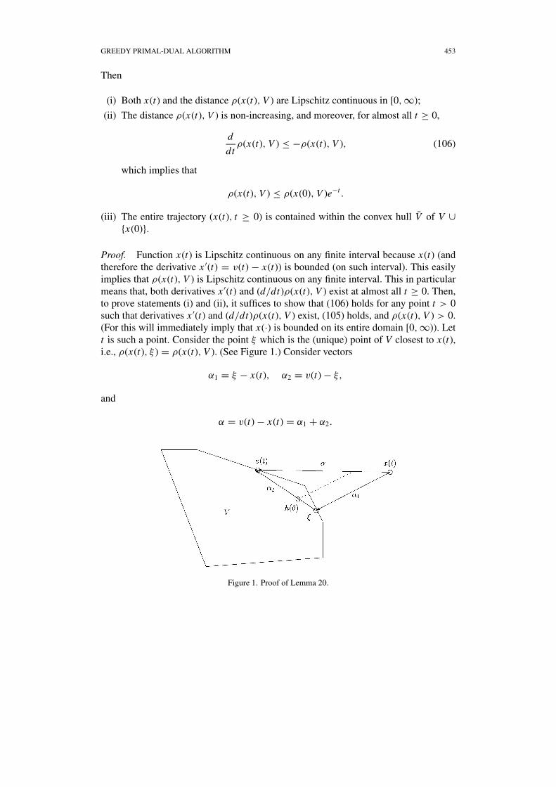
GREEDY PRIMAL-DUAL ALGORITHM 453
Then
(i) Both x(t) and the distance ρ(x(t), V ) are Lipschitz continuous in [0, ∞);
(ii) The distance ρ(x(t), V ) is non-increasing, and moreover, for almost all t ≥ 0,
d
dtρ(x(t), V ) ≤ −ρ(x(t), V ), (106)
which implies that
ρ(x(t), V ) ≤ ρ(x(0), V )e−t .
(iii) The entire trajectory (x(t), t ≥ 0) is contained within the convex hull V of V ∪{x(0)}.
Proof. Function x(t) is Lipschitz continuous on any finite interval because x(t) (andtherefore the derivative x ′(t) = v(t) − x(t)) is bounded (on such interval). This easilyimplies that ρ(x(t), V ) is Lipschitz continuous on any finite interval. This in particularmeans that, both derivatives x ′(t) and (d/dt)ρ(x(t), V ) exist at almost all t ≥ 0. Then,to prove statements (i) and (ii), it suffices to show that (106) holds for any point t > 0such that derivatives x ′(t) and (d/dt)ρ(x(t), V ) exist, (105) holds, and ρ(x(t), V ) > 0.(For this will immediately imply that x(·) is bounded on its entire domain [0, ∞)). Lett is such a point. Consider the point ξ which is the (unique) point of V closest to x(t),i.e., ρ(x(t), ξ ) = ρ(x(t), V ). (See Figure 1.) Consider vectors
α1 = ξ − x(t), α2 = v(t) − ξ,
and
α = v(t) − x(t) = α1 + α2.
Figure 1. Proof of Lemma 20.
454 STOLYAR
Consider auxiliary linear function
h(θ ) = ξ + α2(θ − t), θ ≥ t,
and note that h(θ ) ∈ V for all sufficiently small increments (θ − t) ≥ 0. Then, we canwrite
d
dtρ(x(t), V ) ≤ d+
dθρ(x(θ ), h(θ )) |θ=t=
− ||α1|| = −ρ(x(t), V ).
The proof of (i) and (ii) is complete. Statement (iii) is a corollary of (ii), becausev(t) ∈ V for almost all t and x(0) ∈ V .
Proof of (32)
If v∗ lies in the interior of V, the statement is obvious. Suppose v∗ lies on the boundaryof V. Let C◦(v∗) denote the cone polar to cone C∗(v∗). (In other words, C◦(v∗) is thecone normal to C∗(v∗) at point 0).
Denote by � the set of all unit length vectors ξ lying on the boundary of C◦(v∗).Let u∗(x) denote the normal projection of x on V, that is the point of V closest to x. Sincecone C◦(v∗) is polar to the normal cone C∗(v∗) (and V is compact), the following holds:
1
δsupξ∈�
||u∗(v∗ + δξ ) − (v∗ + δξ )|| ↓ 0 as δ ↓ 0.
(Otherwise we would be able to construct ξ ∈ � and a convex cone A, containing ξ
in the interior, such that the set v∗ + A intersects with V at a single point v∗. This isimpossible since ξ is an element of the polar cone C◦(v∗)). This in particular impliesthat
supξ∈�
α(u∗(v∗ + δξ ), ξ ) ↓ 0 as δ ↓ 0, (107)
where α(·, ·) denotes the angle between two vectors, and
infξ∈�
||u∗(v∗ + δξ ) − v∗||/δ → 1 as δ ↓ 0. (108)
Now we can finish the proof of (32). Since vector ∇ H (x(t))−q(t) is uniformly bounded,at any time t when its distance to C∗(v∗) is away from 0—namely, it is greater or equal tosome ε1 > 0—the angle between ∇ H (x(t)) − q(t) and C∗(v∗) is bounded away from 0as well. This implies that the angle between ∇ H (x(t))−q(t) and the cone C◦(v∗) is lessthan and bounded away from the right angle π/2. To summarize, if ξ (t) is the vector in �
forming the smallest angle with ∇ H (x(t))−q(t), then p(∇ H (x(t))−q(t), C∗(v∗)) ≥ ε1
GREEDY PRIMAL-DUAL ALGORITHM 455
implies α(∇ H (x(t)) − q(t), ξ (t)) ≤ π/2 − ε3 for some ε3 > 0 (depending on ε1).According to (107) and (108), we can always choose δ > 0 small enough so thatα(u∗(δξ (t)) − v∗, δξ (t)) < ε3/2 and ||u∗(δξ (t))|| ≥ δ/2. Finally, when ρ(∇ H (x(t)) −q(t), C∗(v∗)) ≥ ε1 we have α(∇ H (x(t)) − q(t), u∗(δξ (t)) − v∗) ≤ π/2 − ε3/2 (and,obviously, ‖∇ H (x(t)) − q(t)‖ ≥ ε1), and therefore
B3(t) = maxv∈V
[∇ H (x(t)) − q(t)] · (v − v∗) ≥ [∇ H (x(t)) − q(t)] · (u∗(δξ (t)) − v∗)
≥ ε1(δ/2) sin(π/2 − ε3/2) > 0.
Some elementary facts
Proposition 1. Suppose H (v) is a continuously differentiable concave function withconvex open domain V ⊆ RN , N ≥ 1. Suppose H (v) has same value along the linesegment L connecting two points v(1), v(2) ∈ V . Then, ∇ H (v(1)) = ∇ H (v(2)). (Andthen ∇ H (v) is same for all v ∈ L).
Proof. Suppose ∇ H (v(1)) �= ∇ H (v(2)). Let us pick a non-zero vector ζ ∈ RN suchthat
∇ H(v(1)
) · ζ > ∇ H(v(2)
) · ζ. (109)
Consider function
A(ξ ) = 1
2
[H
(v(1) + ζ ξ
) + H(v(2) − ζ ξ
)],
which is well defined for all sufficiently small real ξ . By concavity of H, for all (small)ξ, A(ξ ) ≤ A(0) = H (v(mid)), where v(mid) = [v(1) + v(2)]/2. On the other hand, by(109), A′(ξ ) > 0. Contradiction completes the proof.
The following fact is standard and is easy to verify directly.
Proposition 2. Suppose V ⊂ RN , N ≥ 1, is a compact set. The multivalued operatorwhich takes a vector ζ ∈ Rn into the set Vζ
.= arg maxv∈V ζ · v is closed. Namely, ifsequences of ζ (i) ∈ RN and v(i) ∈ V, on i = 1, 2, . . . are such that ζ (i) → ζ, v(i) ∈ Vζ (i) ,and v(i) → v, then v ∈ Vζ .
Since V is compact, closedness of the operator implies its upper semicontinuity(cf. [9], Lemma XVI. 5.1). Namely, for any ζ ∈ RN and ε > 0, there exists δ > 0 suchthat ||ζ ′ − ζ || < δ implies Vζ ′ ⊆ {v ∈ V | ρ(v, Vζ ) < ε}.
Acknowledgment
I would like to thank the referees for very useful comments, which helped in improvingpresentation in the paper.
456 STOLYAR
References
[1] M. Andrews, K. Kumaran, K. Ramanan, A.L. Stolyar, R. Vijayakumar and P. Whiting, Providingquality of service over a shared wireless link, IEEE Communications Magazine 39(2) (2001) 150–154.
[2] M. Andrews, L. Qian and A.L. Stolyar, Optimal utility based multi-user throughput allocation subjectto throughput constraints, in: Proceeding of INFOCOM’2005, Miami, March 13–17, 2005.
[3] R. Agrawal and V. Subramanian, Optimality of certain channel aware scheduling policies, in: Proc.of the 40th Annual Allerton Conference on Communication, Control, and Computing, (Monticello,Illinois, USA, October 2002).
[4] J.G. Dai and W. Lin, Maximum pressure policies in stochastic processing networks, OperationsResearch 53(2) (2005) 197–218.
[5] S.N. Ethier and T.G. Kurtz, Markov Processes: Characterization and Convergence, (John Wiley andSons, New York, 1986).
[6] A. Eryilmaz and R. Srikant, Fair resource allocation in wireless networks using queue-length-basedscheduling and congestion control, in: Proceedings of INFOCOM’2005, Miami, March 13–17, 2005.
[7] J.M. Harrison. Brownian Motion and Stochastic Flow Systems, (Wiley, 1985).[8] A. Jalali, R. Padovani and R. Pankaj, Data Throughput of CDMA-HDR, a high efficiency—high data
rate personal communication wireless system, in: Proc. of the IEEE Semiannual Vehicular TechnologyConference, VTC2000-Spring (Tokyo, Japan, May 2000).
[9] L.V. Kantorovich and G.P. Akilov, Functional Analysis, 2nd ed. (Pergamon Press, New York, 1982).[10] F.P. Kelly, A.K. Maullo and D.K.H. Tan, Rate control in communication networks: Shadow prices,
proportional fairness and stability, Journal of the Operational Research Society 49 (1998) 237–252.[11] F.P. Kelly, Fairness and stability of end-to-end congestion control, European Journal of Control 9
(2003) 159–176.[12] T. Klein and H. Viswanathan, Centralized power control for multi-hop wireless networks, (2003),
submitted.[13] S. Karlin, Mathematical Methods in Games, Programming, and Economics (Dover, New York, 1992).[14] S. Liu, T. Basar and R. Srikant, Controlling the Internet: A survey and some new results (2003),
preprint.[15] X. Liu, E.K.P. Chong and N.B. Shroff, A framework for opportunistic scheduling in wireless networks,
Computer Networks 41 (2003) 451–474.[16] S. Low, A duality model of TCP and queue management algorithms, IEEE/ACM Transactions on
Networking 11(4) (2003) 525–536.[17] R.T. Rockafellar, Convex Analysis, Princeton Univ. Press, 1970.[18] R. Srikant, The Mathematics of Internet Congestion Control (Birkhauser, 2004).[19] A.L. Stolyar, On the stability of multiclass queueing networks: A relaxed sufficient condition via
limiting fluid processes, Markov Processes and Related Fields 1(4) (1995) 491–512.[20] A.L. Stolyar, MaxWeight scheduling in a generalized switch: State space collapse and workload
minimization in heavy traffic, Annals of Applied Probability 14(1) (2004) 1–53.[21] A.L. Stolyar, On the asymptotic optimality of the gradient scheduling algorithm for multi-user through-
put allocation, Operations Research 53(1) (2005) 12–25.[22] L. Tassiulas and A. Ephremides, Stability properties of constrained queueing systems and scheduling
policies for maximum throughput in multihop radio networks, IEEE Transactions on AutomaticControl 37 (1992) 1936–1948.
[23] L. Tassiulas and P.P. Bhattacharya, Allocation of interdependent resources for maximal throughput,Commun. Statist.—Stochastic Models 16 (2000) 27–48.
[24] D. Tse and S. Hanly, Multi-access fading channels: Part I: Polymatroid structure, optimal resourceallocation and throughput capacities, IEEE Transactions on Information Theory 44(7) (1998) 2796–2815.
GREEDY PRIMAL-DUAL ALGORITHM 457
[25] P. Viswanath, D. Tse and R. Laroia, Opportunistic beamforming using dumb antennas, IEEE Trans-actions on Information Theory 48(6) (2002) 1277–1294.
[26] J.T. Wen and M. Arcak, A unifying passivity framework for network flow control, IEEE Transactionson Automatic Control 49(2) (2004) 162–174.
[27] E.M. Yeh and A.S. Cohen, Throughput and delay optimal resource allocation in multiaccess fadingchannels, in: Proceedings of ISIT, (Yokohama, Japan, June–July 2003).