Bayesian K-Means as a “Maximization-Expectation”

Algorithm

Kenichi Kurihara

kurihara@mi.cs.titech.ac.jp

Department of Computer Science

Tokyo Institute of Technology, Japan

Max Welling

welling@ics.uci.edu

Department of Computer Science

UC Irvine, CA 92697-3425, US

June 15, 2006

Abstract

We introduce a new class of “maximization expectation” (ME) algorithms wherewe maximize over hidden variables but marginalize over random parameters. Thisreverses the roles of expectation and maximization in the classical EM algorithm. Inthe context of clustering, we argue that the hard assignments from the maximizationphase open the door to very fast implementations based on data-structures such askd-trees and conga-lines. The marginalization over parameters ensures that weretain the ability to select the model structure (i.e. number of clusters). As animportant example we discuss a top-down “Bayesian k-means” algorithm and abottom-up agglomerative clustering algorithm. In experiments we compare thesealgorithms against a number of alternative algorithms that have recently appearedin the literature.

1 Introduction

K-means is undoubtedly one of the workhorses of machine learning. Faced with theexponential growth of data researchers have recently started to study strategies to speedup k-means and related clustering algorithms. Most notably, methods based on kd-trees[Pelleg and Moore, 1999, Moore, 1998, Zhang et al., 1996, Verbeek et al., 2003] andmethods based on the triangle inequality [Moore, 2000, Elkan, 2003] have been verysuccessful in achieving orders of magnitude improved efficiency.

Another topic of intense study has been to device methods that automatically deter-mine the number of clusters from the data [Pelleg and Moore, 1999, Hamerly and Elkan,2003]. One of the most promising algorithms in this respect is based on the “variationalBayesian” (VB) paradigm [Attias, 2000, Ghahramani and Beal, 2000]. Here distributionsover cluster assignments and distributions over stochastic parameters are alternatinglyestimated in an EM-like fashion. Unfortunately, it is difficult to apply the speed-uptricks mentioned above to this algorithm, at least without introducing approximations.One of the main goals in this paper is to propose a modification of VB-clustering thatcombines model selection with the possibility for fast implementations.

The technique we propose is an instance of a new class of “ME algorithms” thatreverses the roles of expectation and maximization in the EM algorithm. Alternatively,it can be viewed as a special case of the VB framework where expectation over hidden

1

variables is replaced with maximization. We show that convergence is guaranteed byderiving the objective that is optimized by these iterations.

In the context of clustering we discuss a ME algorithm that is very similar tok-means but uses a full covariance and an upgraded “distance” to penalize overlycomplex models. We also derive an alternative agglomerative clustering algorithm.Both algorithms can be implemented efficiently using kd-trees and conga-lines respec-tively. Experimentally, we see no performance drops relative to VB but at the sametime we demonstrate significant speedup factors. Our software is publicly available athttp://mi.cs.titech.ac.jp/kurihara/bkm.html

2 Maximization-Expectation Algorithms

Consider a probabilistic model, P (x, z, θ), with observed random variables (RVs), x,hidden RVs , z, and parameters, θ (which are assumed random as well). We adopt theconvention that RVs are called “hidden” if there is a hidden-RV for each data-case (e.g.cluster assignment variables), while RVs are called parameters if their number is fixedor needs to be inferred from the data (e.g. cluster centroids).

Given a dataset D, a typical task in machine learning is to compute posterior ormarginal probabilities such as p(z|D), p(θ|D) or p(D). The former can be used todetermine for instance a clustering of the data, when z represents cluster assignmentvariables. It is not untypical that exact expressions for these quantities can not bederived and approximate methods become necessary. We will now review a number ofapproaches based on alternating model estimation.

A standard approach is to represent the distribution using samples. The canonicalexample being a Gibbs sampler which alternatingly samples,

θ ∼ p(θ|z,D) ↔ z ∼ p(z|θ,D). (1)

Instead of sampling, one can fit factorized variational distributions to the exactdistribution, i.e. p(θ, z|D) ≈ q(θ)q(z). This “variational Bayesian” (VB) approximation[Attias, 2000, Ghahramani and Beal, 2000] alternatingly estimates these distributionsby minimizing the KL-divergence, KL[q(θ)q(z)||p(θ, z|D)] between the approximationand the exact distribution. This results in the updates,

q(θ) ∝ exp(E[log p(θ, z,D)]q(z)) ↔ q(z) ∝ exp(E[log p(θ, z,D)]q(θ)). (2)

Instead of maintaining a distribution over parameters, one could decide to estimate aMAP value for θ. To find this MAP value, θ∗, one can use the expectation-maximizationalgorithm (EM) to alternatingly compute,

θ∗ = argmaxθ

E[log(p(θ, z,D)]q(z) ↔ q(z) = p(z|θ∗,D). (3)

This turns out to be special case of the VB formalism by approximating the posterioras q(θ) = δ(θ, θ∗), where δ(·) is a delta function. Finally, one can also choose to usepoint-estimates for both θ and z, which is known as “iterative conditional modes” (ICM).In this case we iteratively maximize the posterior distributions, p(θ|z,D) and p(z|θ,D)which is equivalent to,

2

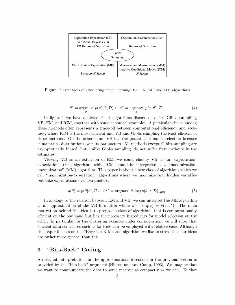
Figure 1: Four faces of alternating model learning: EE, EM, ME and MM algorithms

θ∗ = argmaxθ

p(z∗, θ,D) ↔ z∗ = argmaxz

p(z, θ∗,D). (4)

In figure 1 we have depicted the 4 algorithms discussed so far, Gibbs sampling,VB, EM, and ICM, together with some canonical examples. A particular choice amongthese methods often represents a trade-off between computational efficiency and accu-racy, where ICM is the most efficient and VB and Gibbs sampling the least efficient ofthese methods. On the other hand, VB has the potential of model selection becauseit maintains distributions over its parameters. All methods except Gibbs sampling areasymptotically biased, but, unlike Gibbs sampling, do not suffer from variance in theestimates.

Viewing VB as an extension of EM, we could classify VB as an “expectation-expectation” (EE) algorithm while ICM should be interpreted as a “maximization-maximization” (MM) algorithm. This paper is about a new class of algorithms which wecall “maximization-expectation” algorithms where we maximize over hidden variablesbut take expectations over parameters,

q(θ) = p(θ|z∗,D) ↔ z∗ = argmaxz

E[log(p(θ, z,D)]q(θ). (5)

In analogy to the relation between EM and VB, we can interpret the ME algorithmas an approximation of the VB formalism where we use q(z) = δ(z, z∗). The mainmotivation behind this idea is to propose a class of algorithms that is computationallyefficient on the one hand but has the necessary ingredients for model selection on theother. In particular for the clustering example under consideration, we will show thatefficient data-structures such as kd-trees can be employed with relative ease. Althoughthis paper focuses on the “Bayesian K-Means” algorithm we like to stress that our ideasare rather more general than this.

3 “Bits-Back” Coding

An elegant interpretation for the approximations discussed in the previous section isprovided by the “bits-back” argument [Hinton and van Camp, 1993]. We imagine thatwe want to communicate the data to some receiver as compactly as we can. To that

3

end, we first learn a probabilistic model for the data (say a “mixture of Gaussians”(MoG) model). We use the internal representation of the hidden units to encode thedata-vectors. For instance, the cluster assignments in a MoG can be used to vector-quantize the data-vectors. To communicate the data, we first send the parameters ofthe model that we learned. Next, we send the hidden representation for each data-vector.The receiver will predict the data vectors from this information, but since the code wesend is “lossy” we still need to send (hopefully small) error corrections. Note that thesender and receiver need to agree on a quantization level (or resolution) with which theymeasure parameters, code vectors and data vectors. Given such a quantization level,it takes less bits to encode small error terms than to encode the entire data vectorsthemselves resulting in the desired compression.

The reason that the optimal compression results in model selection follows from thefact that the number of parameters that are sent is constant (they have to be sendonly once) while the hidden representation and the error terms scale with the numberof data-vectors. Hence, when we have a few data vectors to communicate it doesn’tpay back to train a complicated model: the bits needed to send the model parametersmay be more expensive than sending the data vectors directly. On the other hand,using a complicated model to encode the data is warranted if we have to communicatelots of data vectors (assuming there is structure to be found in the data). It is thisdelicate interplay that determines the complexity of the model that results in optimalcompression.

According to Shannon [1948] we need log2 p(θ|M) bits to encode the parameters,log2 p(z|θ,M) bits to encode the hidden representation z (e.g. cluster assignments) andlog2 p(x|z, θ,M) to encode the error terms for a model “M”. Although one is inclinedto think that the optimal model and encoding results by minimizing the sum of the 3terms over z and θ (called energy), one can in fact do better. Consider for instance thecase that two choices for z both minimize the energy. Since both options are optimal,one can use this additional freedom to encode some side information (or future datavectors). In effect, we got some bits refunded. More generally, we can use a distributionq(z, θ) to choose which z and θ we use for the encoding. This will result in an an averageenergy term of,

E[q] =

∫

dθ∑

z

q(z, θ)(log2 P (x|z, θ,M) + log2 P (z|θ,M) + log2 P (θ|M)).

However, the amount of information contained in our stochastic choices of the codeand model parameters is,

H[q] = −∫

dθ∑

z

q(z, θ) log2 q(z, θ). (6)

Hence, the total amount of bits needed to communicate the data becomes F [q] =E[q] − H[q] which is equal to the negative of the logarithm of the marginal likelihood(or evidence).

We are now ready to interpret the approximations made by the 4 algorithms in figure1. The EM algorithm uses stochastic choices for the code vectors z but maximizes

4

over the parameters θ declining the refund possible from random choices. The VBformalism uses stochastic choices for both z and θ but uses a factorized distributionq(z, θ) = q(z)q(θ) to choose them which is also suboptimal1. ICM will not receive anybits back from either z or θ because it maximizes over both of them. Finally, in theME formalism we receive bits back from the parameters θ but since we optimize overthe encoding z we decline a potential refund which we would have obtained throughstochastic choices. The argument we are making in this paper is that this sacrifice willhelp us develop computationally efficient algorithms.

4 The Large N Limit

In the previous sections we have viewed the ME procedure as either an approximationto Bayesian model selection or as an approximation to the bits-back coding principle.In this section we will derive the result that for large N we recover the well knownBayesian information criterion (BIC), or equivalently the maximum description length(MDL) penalty.

The cost function (free energy) that the ME algorithm minimizes is given by thefollowing bound on the negative marginal likelihood,

F(z,K) = −E[log p(D, θ, z ′)]q(θ)δ(z′ ,z) −H[q(θ)] (7)

= − log p(D) +KL[q(θ)δ(z ′, z)||p(θ, z′|D)]

≥ − log p(D).

This free energy can be rewritten as,

F(z,K) =

∫

dθ [−q(θ) log p(D, z|θ) − q(θ) log p(θ) + q(θ) log p(θ)] . (8)

We use the result proven by Wang and Titterington [2005], that for N → ∞ theparameters converge to the maximum likelihood estimates, θN → θML. It was also shownthat the distribution q(θ) is asymptotically normal with a covariance matrix Cov(θ) =Σ/N . Moreover, the covariance Σ is smaller than the inverse Fisher information matrix:Σ I−1

F (meaning that I−1F − Σ is non-negative definite). Expanding log p(D, z|θ) up

to second order we find,

log p(D, z|θ) ≈ log p(D, z|θML) +N

2(θ − θML)T IF (θ − θML) (9)

Using that E[(θ − θML)(θ− θML)T ] = Σ/N and retaining only terms that grow withN we find for the first term of Eqn.8,

log p(D, z|θ) ≈ log p(D, z|θML). (10)

Using a similar approximation for the second term in Eqn.8 but observing that theHessian for log p(θ) does not grow with N we find that it can be ignored. The thirdterm represents the entropy of q(θ) which asymptotically becomes

1Note that one should in fact expect strong dependencies between z and θ.

5

H(θ) ≈ −M2

logN (11)

where M is the number of parameters in the model. Putting everything together wefind,

F(z,K) ≈ log p(D, z|θML) − M

2logN (12)

which matches the BIC/MDL criterion. Note however, that for small N the ME ap-proximation is different from the BIC/MDL criterion because it retains all orders inN .

5 The Hard Assignment Approximation for Bayesian Clus-

tering

In this section we will consider a specific example of the ME algorithm in the contextof clustering.

Let xn, n = 1, ..., N be a vector of IID continuous-valued observations in Ddimensions. For each data-case we define a cluster assignment variable, zn ∈ [1, ...,K].We assume that the data has been generated following a mixture of Gaussians,

p(xn, zn|α,µ,Ω) = N (xn|zn,µ,Ω) M(zn|α) (13)

where µ are the cluster means, Ω the inverse cluster covariances and α the mixing co-efficients. N (·) represents a normal distribution and M(·) a multinomial (or discrete)distribution. We place conjugate priors on the parameters and subsequently marginal-ized them out to give,

p(xn, zn) =

∫

dµdΩdα N (xn|zn,µ,Ω) M(zn|α) D(α|φ0) N (µ|m0, ξ0Ω) W(Ω|η0, B0).

(14)where D(·) is a Dirichlet distribution and W(·) is a Wishart distribution. The priors de-pend on some (non-random) hyper-parameters, m0, φ0, ξ0, η0, B0. Uninformative priorsare covered in appendix A.

For clustering, we are interested in the posterior distribution p(z|D), where D de-notes the data-set and z are binary assignment variables for each data-case. In theapproximation we propose we replace the full posterior with the following factorizedform,

p(z,θ|D) ≈ q(θ) δ(z, z∗) (15)

that is we maintain a distribution over parameters, but settle for a point-estimate of theassignment variables. Minimizing the KL-divergence between this approximate posteriorand the exact posterior, KL[q(θ)δ(z, z∗)||p(z,θ|D)], over q(θ) we find,

6

q(µ,Ω,α) =

[

K∏

c=1

N (µc|mc, ξcΩc) W(Ωc|ηc, Bc)

]

D(α|φc) (16)

where

ξc = ξ0 +Nc mc =Ncxc + ξ0m0

ξcηc = η0 +Nc

Bc = B0 +NcSc +Ncξ0ξc

(xc −m0)(xc −m0)T

φ = φ1, ..., φK φc = φ0 +Nc (17)

and where Nc denotes the number of data-cases in cluster c, xc is the sample mean ofcluster c, and Sc is its sample covariance.

The main simplification that has resulted from the approximation in Eqn.15 is thatthis distribution now factorizes over the clusters. Using this and Eqn.7 we derive thefollowing bound on the log evidence (or “free energy”),

F(z,K) =

K∑

c=1

[

DNc

2log π +

1

2log

ξcξ0

+ηc

2log det(Bc) −

η0

2log det(B0)

− logΓD(ηc

2 )

ΓD(η0

2 )+

1

Klog

Γ(N +Kφ0)

Γ(Kφ0)− log

Γ(φc)

Γ(φ0)

]

(18)

where ΓD(x) = πD(D−1)

4∏D

i=1 Γ(x+ 1−i2 ) and Γ(·) the Gamma function. We observe that

this objective also nicely factorizes into a sum of terms, one for each cluster. Unlike themaximum likelihood criterion, this objective automatically penalizes overly complexmodels. Our task is to minimize Eqn.18 jointly over assignment variables zn, n = 1..Nand K, the number of clusters.

6 The ME-Algorithm for Clustering: “Bayesian K-Means”

In this paper we study two approaches to minimizing the cost Eqn.18. The one which wediscuss in this section is a Bayesian variant of k-means (BKM), which is an instance ofthe more general class of “ME-algorithms”. In section 7 we will discuss an agglomerativeclustering algorithm.

From Eqn.5 we see that the ME algorithm iteratively maximizes E[log(p(θ, z,D)]q(θ),where p(θ, z,D) can be derived from Eqn.14 and q(θ) is given by Eqn.16. This leads(after some algebra) to the following iterative “labeling cost”,

7

CBKM =∑

n

γzn(xn) with (19)

γzn(xn) =

ηzn

2(xn −mzn

)TB−1zn

(xn −mzn)

+1

2log det(Bzn

) +D

2ξzn

− 1

2

D∑

d=1

Ψ

(

ηzn+ 1 − d

2

)

− Ψ(φzn).

where Ψ(x) = ∂ log Γ(x)∂x is the “digamma” function. We recognize γzn

(xn) as the Maha-lanobis distance plus some constant correction term. Due to this extra constant γ(x)can not be interpreted as a proper distance.

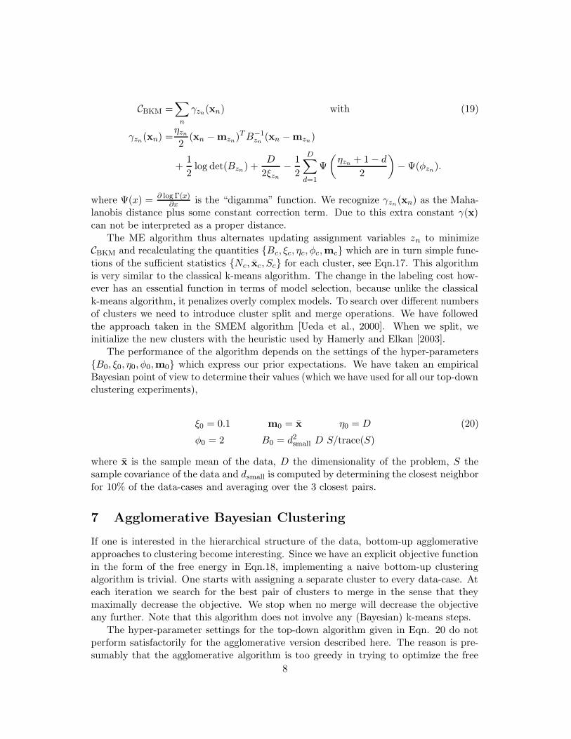
The ME algorithm thus alternates updating assignment variables zn to minimizeCBKM and recalculating the quantities Bc, ξc, ηc, φc,mc which are in turn simple func-tions of the sufficient statistics Nc, xc, Sc for each cluster, see Eqn.17. This algorithmis very similar to the classical k-means algorithm. The change in the labeling cost how-ever has an essential function in terms of model selection, because unlike the classicalk-means algorithm, it penalizes overly complex models. To search over different numbersof clusters we need to introduce cluster split and merge operations. We have followedthe approach taken in the SMEM algorithm [Ueda et al., 2000]. When we split, weinitialize the new clusters with the heuristic used by Hamerly and Elkan [2003].

The performance of the algorithm depends on the settings of the hyper-parametersB0, ξ0, η0, φ0,m0 which express our prior expectations. We have taken an empiricalBayesian point of view to determine their values (which we have used for all our top-downclustering experiments),

ξ0 = 0.1 m0 = x η0 = D (20)

φ0 = 2 B0 = d2small D S/trace(S)

where x is the sample mean of the data, D the dimensionality of the problem, S thesample covariance of the data and dsmall is computed by determining the closest neighborfor 10% of the data-cases and averaging over the 3 closest pairs.

7 Agglomerative Bayesian Clustering

If one is interested in the hierarchical structure of the data, bottom-up agglomerativeapproaches to clustering become interesting. Since we have an explicit objective functionin the form of the free energy in Eqn.18, implementing a naive bottom-up clusteringalgorithm is trivial. One starts with assigning a separate cluster to every data-case. Ateach iteration we search for the best pair of clusters to merge in the sense that theymaximally decrease the objective. We stop when no merge will decrease the objectiveany further. Note that this algorithm does not involve any (Bayesian) k-means steps.

The hyper-parameter settings for the top-down algorithm given in Eqn. 20 do notperform satisfactorily for the agglomerative version described here. The reason is pre-sumably that the agglomerative algorithm is too greedy in trying to optimize the free

8

Top-Down Bayesian K-Means

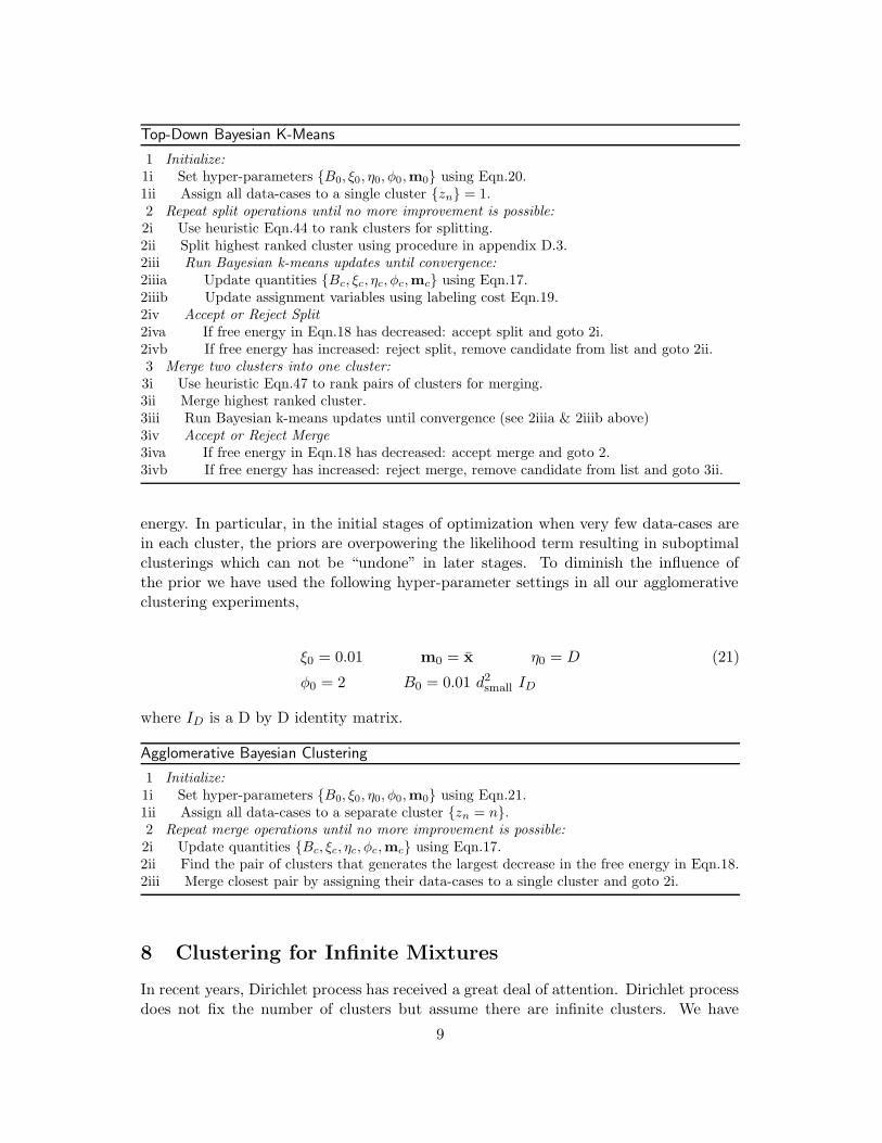
1 Initialize:1i Set hyper-parameters B0, ξ0, η0, φ0,m0 using Eqn.20.1ii Assign all data-cases to a single cluster zn = 1.2 Repeat split operations until no more improvement is possible:2i Use heuristic Eqn.44 to rank clusters for splitting.2ii Split highest ranked cluster using procedure in appendix D.3.2iii Run Bayesian k-means updates until convergence:2iiia Update quantities Bc, ξc, ηc, φc,mc using Eqn.17.2iiib Update assignment variables using labeling cost Eqn.19.2iv Accept or Reject Split2iva If free energy in Eqn.18 has decreased: accept split and goto 2i.2ivb If free energy has increased: reject split, remove candidate from list and goto 2ii.3 Merge two clusters into one cluster:3i Use heuristic Eqn.47 to rank pairs of clusters for merging.3ii Merge highest ranked cluster.3iii Run Bayesian k-means updates until convergence (see 2iiia & 2iiib above)3iv Accept or Reject Merge3iva If free energy in Eqn.18 has decreased: accept merge and goto 2.3ivb If free energy has increased: reject merge, remove candidate from list and goto 3ii.

energy. In particular, in the initial stages of optimization when very few data-cases arein each cluster, the priors are overpowering the likelihood term resulting in suboptimalclusterings which can not be “undone” in later stages. To diminish the influence ofthe prior we have used the following hyper-parameter settings in all our agglomerativeclustering experiments,

ξ0 = 0.01 m0 = x η0 = D (21)

φ0 = 2 B0 = 0.01 d2small ID

where ID is a D by D identity matrix.

Agglomerative Bayesian Clustering

1 Initialize:1i Set hyper-parameters B0, ξ0, η0, φ0,m0 using Eqn.21.1ii Assign all data-cases to a separate cluster zn = n.2 Repeat merge operations until no more improvement is possible:2i Update quantities Bc, ξc, ηc, φc,mc using Eqn.17.2ii Find the pair of clusters that generates the largest decrease in the free energy in Eqn.18.2iii Merge closest pair by assigning their data-cases to a single cluster and goto 2i.

8 Clustering for Infinite Mixtures

In recent years, Dirichlet process has received a great deal of attention. Dirichlet processdoes not fix the number of clusters but assume there are infinite clusters. We have

9

discussed a model selection using the free energy which search for the optimal numberof clusters. However, here we show it is straightforward to extend our models to infinitemixtures.

Following Griffiths and Ghahramani [2006], we define partition. So far, we have useda notation assignment to specify each object to one cluster. For example, assignments(z1, z2, z3) = (1, 1, 2) means x1, x2 and x3 are assigned to cluster 1, 1 and 2 respectively.If 1 and 2 are just labels, (1, 1, 2) would be equal to (2, 2, 1). A partition denotes a setof equivalent assignments. In this case, partition [z] is equal to set (1, 1, 2), (2, 2, 1).

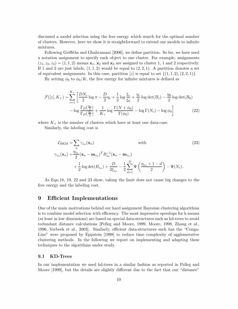
By setting φ0 to φ0/K, the free energy for infinite mixtures is defined as

F([z],K+) =

K+∑

c=1

[

DNc

2log π − D

2ηc +

1

2log

ξcξ0

+ηc

2log det(Bc) −

η0

2log det(B0)

− logΓD(ηc

2 )

ΓD(η0

2 )+

1

K+log

Γ(N + φ0)

Γ(φ0)− log Γ(Nc) − log φ0

]

(22)

where K+ is the number of clusters which have at least one data-case.Similarly, the labeling cost is

CBKM =∑

n

γzn(xn) with (23)

γzn(xn) =

ηzn

2(xn −mzn

)TB−1zn

(xn −mzn)

+1

2log det(Bzn

) +D

2ξzn

− 1

2

D∑

d=1

Ψ

(

ηzn+ 1 − d

2

)

− Ψ(Nc).

As Eqn.18, 19, 22 and 23 show, taking the limit does not cause big changes to thefree energy and the labeling cost.

9 Efficient Implementations

One of the main motivations behind our hard assignment Bayesian clustering algorithmsis to combine model selection with efficiency. The most impressive speedups for k-means(at least in low dimensions) are based on special data-structures such as kd-trees to avoidredundant distance calculations [Pelleg and Moore, 1999, Moore, 1998, Zhang et al.,1996, Verbeek et al., 2003]. Similarly, efficient data-structures such has the “Conga-Line” were proposed by Eppstein [1998] to reduce time complexity of agglomerativeclustering methods. In the following we report on implementing and adapting thesetechniques to the algorithms under study.

9.1 KD-Trees

In our implementation we used kd-trees in a similar fashion as reported in Pelleg andMoore [1999], but the details are slightly different due to the fact that our “distance”

10

function in Eqn.19 is different2.A kd-tree is a data-structure where every node is associated with a hyper-rectangle h

containing a subset of data-cases. Each node stores the sufficient statistics Nh, xh, Sh ofthe data-cases in its corresponding hyper-rectangle. The tree is constructed recursivelyby dividing the hyper-rectangles in two smaller hyper-rectangles and associating them(and their sufficient statistics) with the child nodes of the kd-tree.

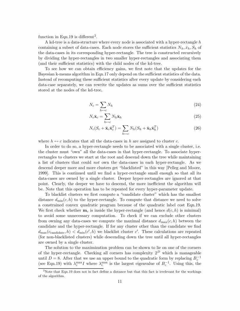
To see how we can obtain efficiency gains, we first note that the updates for theBayesian k-means algorithm in Eqn.17 only depend on the sufficient statistics of the data.Instead of recomputing these sufficient statistics after every update by considering eachdata-case separately, we can rewrite the updates as sums over the sufficient statisticsstored at the nodes of the kd-tree,

Nc =∑

h↔c

Nh (24)

Ncxc =∑

h↔c

Nhxh (25)

Nc(Sc + xcxTc ) =

∑

h↔c

Nh(Sh + xhxTh ) (26)

where h↔ c indicates that all the data-cases in h are assigned to cluster c.In order to do so, a hyper-rectangle needs to be associated with a single cluster, i.e.

the cluster must “own” all the data-cases in that hyper-rectangle. To associate hyper-rectangles to clusters we start at the root and descend down the tree while maintaininga list of clusters that could not own the data-cases in each hyper-rectangle. As wedescend deeper more and more clusters get “blacklisted” in this way [Pelleg and Moore,1999]. This is continued until we find a hyper-rectangle small enough so that all itsdata-cases are owned by a single cluster. Deeper hyper-rectangles are ignored at thatpoint. Clearly, the deeper we have to descend, the more inefficient the algorithm willbe. Note that this operation has to be repeated for every hyper-parameter update.

To blacklist clusters we first compute a “candidate cluster” which has the smallestdistance dmin(c, h) to the hyper-rectangle. To compute that distance we need to solvea constrained convex quadratic program because of the quadratic label cost Eqn.19.We first check whether mc is inside the hyper-rectangle (and hence d(c, h) is minimal)to avoid some unnecessary computation. To check if we can exclude other clustersfrom owning any data-cases we compute the maximal distance dmax(c, h) between thecandidate and the hyper-rectangle. If for any cluster other than the candidate we finddmax(ccandidate, h) < dmin(c

′, h) we blacklist cluster c′. These calculations are repeated(for non-blacklisted clusters) while descending down the tree until all hyper-rectanglesare owned by a single cluster.

The solution to the maximization problem can be shown to lie on one of the cornersof the hyper-rectangle. Checking all corners has complexity 2D which is manageableuntil D = 8. After that we use an upper bound to the quadratic form by replacing B−1

c

(see Eqn.19) with λmaxc I where λmax

c is the largest eigenvalue of B−1c . Using this, the

2Note that Eqn.19 does not in fact define a distance but that this fact is irrelevant for the workings

of the algorithm.

11

problem becomes axis aligned and can be easily solved separately for each dimension.We have also implemented the same strategy to lower bound the minimization problem,using the smallest eigenvalue instead.

9.2 Conga Lines

Conga line data-structures were proposed by Eppstein [1998] to speed up agglomerativeclustering algorithm from O(N 3) to O(N 2 log(N)). The basic idea is to maintain achanging partition of the data-set, where each partition is associated with a directedgraph consisting of a collection of paths. There are O(N) edges and the closest pair willalways be represented by some edge in this collection. The data-structure gets updated,i.e. new partitions and graphs are formed if we remove two clusters and insert the newlymerged cluster. It can be shown that these basic operations take O(N log(N)) timeinstead of the usual O(N 2) for naive implementations. Experimental results on speedupfactors are reported in section 11.

10 Other Instances of the ME Algorithm

So far, we have described the Bayesian k-means algorithm and agglomerative Bayesianclustering. However, it is straightforward to extend the ideas to clustering with discreteattributes. In section 11 we report on some experiments with multinomial distributionsand product of Bernoullis distributions in addition to Gaussian distributions.

The derivation of the relevant quantities are detailed in appendix B and C. Thetop-down and agglomerative algorithms of these models are the same as the algorithmsdescribed in section 6 and 7 with the free energy and the labelling costs replaced bythe ones for these models. Although the labelling costs, Eqn.37 and 43, are in factdifferent than Eqn.19, it is still possible to apply kd-tree data-structures to speed upthe algorithm. Empirical speedup factors are shown in section 11.

11 Experimental Results

In this section, we will show experimental results on a number of synthetic and realdatasets. We will also show the speedup between naive ME algorithms and ME algo-rithms using kd-trees and conga-lines.

11.1 Synthetic Data

In our first experiment we compared Bayesian k-means (BKM) with G-means (softwareobtained from Hamerly and Elkan [2003]), k-means+BIC [see also Pelleg and Moore,2000], mixture of Gaussians (MoG) + BIC and variational Bayesian learning for mix-tures of Gaussians (VBMG) [Attias, 2000, Ghahramani and Beal, 2000]. K-means+BIC,mixtures of Gaussians+BIC and VBMG use the same split and merge strategy as BKM,but different penalty terms to control the number of clusters. These algorithms weretested on a number of synthetic datasets that were generated similarly to Hamerly andElkan [2003]. For each synthetic dataset, we sampled K centroids and stds. such that

12

no two clusters are closer than τ × (the sum of two stds.)/2. After we generated 10datasets of size N , we multiplied the data within each cluster with a random matrix togive them full covariance structure. Figure 2 shows some typical results for BKM onthree random datasets with τ = 0.1, 0.5 and 2.

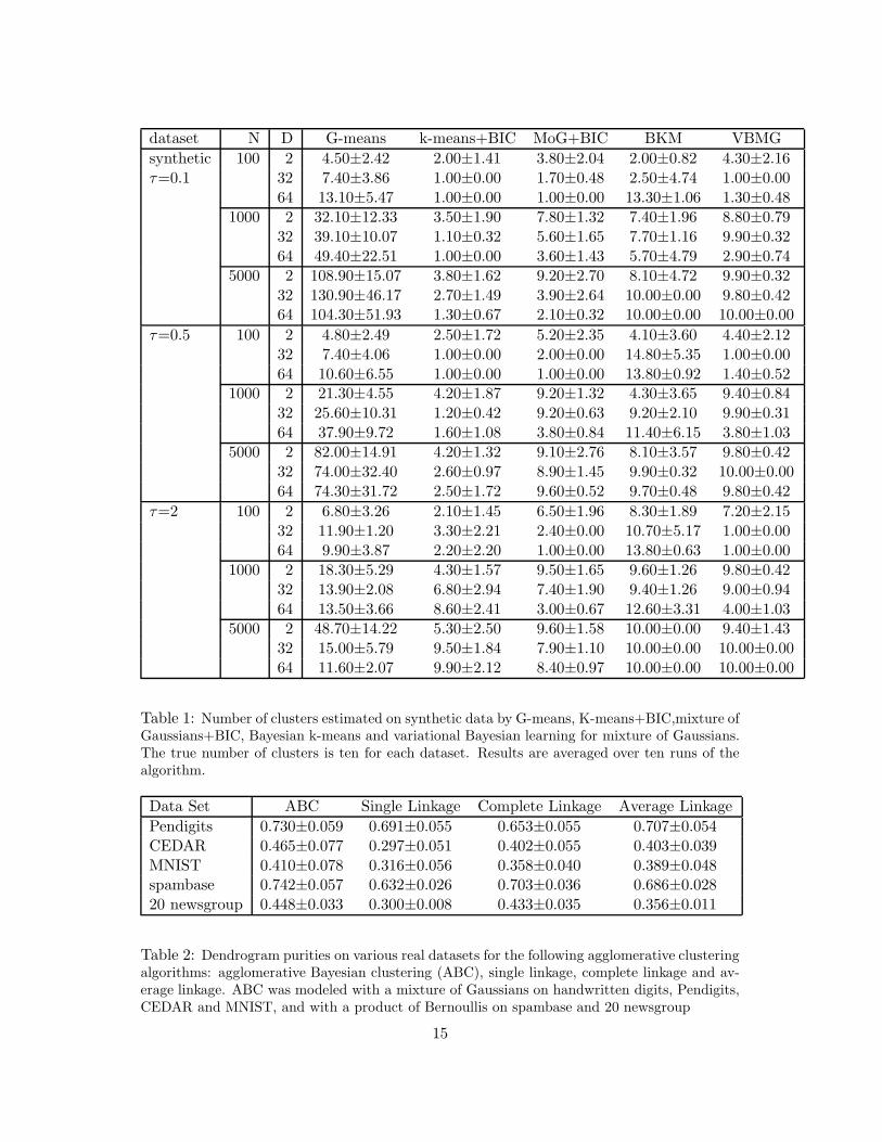
Table 1 shows the results of this experiment. We set K to 10. Therefore, the moreclose to 10, the better a result is. It should come as no surprise that BKM, VBMG andMoG+BIC outperform G-means and k-means+BIC since the latter assume isotropiccovariance. Between BKM, VBMG and MoG+BIC it seems hard to discern significantdifference in performance in these experiments.

We note however that the speedup for BKM is exact while speedup for MoG+BICis approximate [Moore, 1998] and no speedup is currently available for VBMG. Theperformance of the algorithms VBMG and BKM also depend on the setting of thehyper-parameters. The freedom to choose the hyper-parameters is an additional sourceof flexibility. Certainly, when good priors can be specified this should be helpful. In theexperiments reported here we did not make an attempt to improve results by specifyingpriors on a case by case basis, but instead used the empirical Bayesian “rule of thumb”(Eqns.20 and 21) for all experiments. Note that BIC can be derived as the “large-N”limit of both VBMG and BKM (see section 4).

11.2 Real Data

Next, we evaluated agglomerative Bayesian clustering (ABC) against the following tra-ditional agglomerative clustering methods: single, complete and average linkages. Weran these algorithms on real datasets: Pendigits, CEDAR dataset, MNIST dataset, UCIspambase dataset and 20 newsgroups dataset. Pendigits, CEDAR and MNIST datasetsare handwritten digits (0-9) data, and they have 16, 64 and 784 dimensions respectively.Following Hamerly and Elkan [2003], we applied a random projection to the MNISTdataset to reduce the dimension to 50. From the 20 newsgroup dataset, we used onlyrec.autos, rec.sport.baseball, rec.sport.hockey and sci.space categories and chose 50 fea-tures using mutual information. The spambase and the 20 newsgroups datasets werebinarized. ABC used a MoG on the handwritten digits and a product of Bernoullis onthe spambase and 20 newsgroup datasets.

Table 2 shows the results. For each dataset, we created 10 random subsets. Each ofthe handwritten digits datasets contains 100 data-cases. Spambase and 20 newsgroupcontain 200 and 240 data-cases respectively. We evaluated dendrograms with dendro-gram purity which represents how well a dendrogram clusters the known labels. Oneach dataset ABC built the highest purity dendrogram.

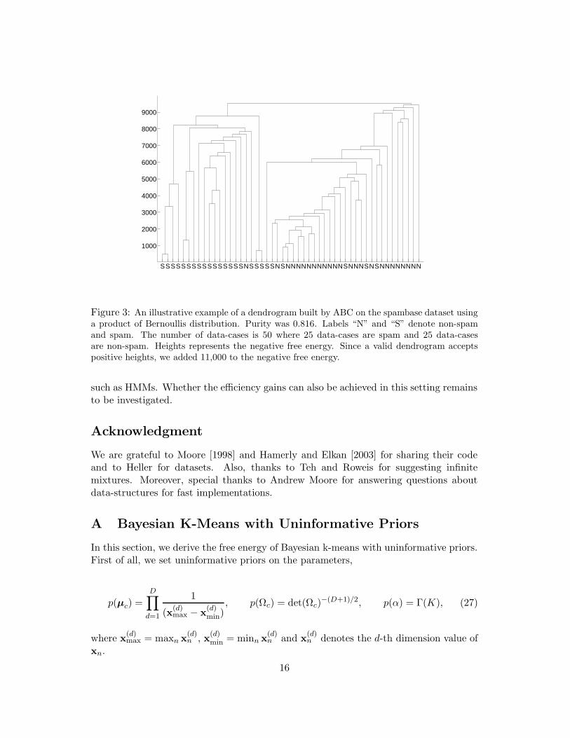
Figure 3 is an illustrative example of a dendrogram for a small subset of spambase.We used 50 data-cases only (25 spam cases, “N”, and 25 non-spam cases, “S”) so thatevery label can be plotted on the x-axis. The purity was 0.816 for this example. Theheight of each linkage represents the negative free energy. Since a valid dendrogramaccepts positive heights, we added 11,000 to the negative free energy.

Finding the correct number of clusters (even approximately) was unsuccessful usingthe hyper-parameter settings in Eqn.21 for each of the handwritten digits datasets.However, the results for the spambase and 20 newsgoups datasets were much better:ABC found K = 2.50 ± 0.53 for spambase and K = 2.0 ± 0.0 for 20 newsgroups.

13

Figure 2: Typical results for BKM for various values of τ = 0.1, 0.5, 2. The true K is equal toten. In these plots, BKM found eight, nine and ten clusters respectively. Since some ellipses aretoo small or too large, they are invisible.

Since we expect 2 groups of spam and non-spam and 3 to 4 groups in the 20 newsgroups(rec.sport.baseball and rec.sport.hockey are probably closely related) this is a reasonableoutcome.

11.3 Efficient implementations

Finally, we compared naive ME algorithms with efficient implementations using kd-treesand conga-lines. For the BKM + kd-trees experiment we varied one parameter at a timeand used default values of N = 20000, D = 2, τ = 3 and K = 5 to sample data. Anode in a kd-tree is declared a leaf if the number of data-cases in the node is less than1000 (the remaining points are treated individually). In the experiments with ABC +conga-lines, we vary N and use D = 2, τ = 3 and K = 10. For the multinomial ME(MME) + kd-trees, we set default values, N = 10000 and D = 8, and varied N and D.

Figure 4 shows the speedup factors. For BKM, speedup increases very fast with N(factor of 67 at N = 80000 ), moderately fast with τ (less overlap helps to blacklistcompeting clusters) and decreases surprisingly slow with dimension (factor of 3.6 in 256dimensions at N = 20000). ABC using the conga-lines is only slightly faster than thenaive implementation due to large overhead but this clearly becomes more significantwith growing N . MME also achieved speedup using kd-trees, but not as significant asBKM.

12 Conclusion

The contributions of this paper are twofold. Firstly a new class of algorithms is intro-duced that reverses the roles of “expectation” and “maximization” in the traditional EMalgorithm. This combines the potential for model selection (because we integrate overthe parameters) with fast implementations (because hard assignments are well suited forefficient data-structures such as kd-trees). Secondly, we have implemented and studiedone possible application of this idea in the context of clustering. Explicit algorithms werederived and experimentally tested for bottom-up Bayesian agglomerative clustering andtop-down Bayesian k-means clustering.

Although we have explored these ideas in the simplest possible context, namelyclustering, the proposed techniques seem to readily generalize to more complex models

14

dataset N D G-means k-means+BIC MoG+BIC BKM VBMG

synthetic 100 2 4.50±2.42 2.00±1.41 3.80±2.04 2.00±0.82 4.30±2.16τ=0.1 32 7.40±3.86 1.00±0.00 1.70±0.48 2.50±4.74 1.00±0.00

64 13.10±5.47 1.00±0.00 1.00±0.00 13.30±1.06 1.30±0.481000 2 32.10±12.33 3.50±1.90 7.80±1.32 7.40±1.96 8.80±0.79

32 39.10±10.07 1.10±0.32 5.60±1.65 7.70±1.16 9.90±0.3264 49.40±22.51 1.00±0.00 3.60±1.43 5.70±4.79 2.90±0.74

5000 2 108.90±15.07 3.80±1.62 9.20±2.70 8.10±4.72 9.90±0.3232 130.90±46.17 2.70±1.49 3.90±2.64 10.00±0.00 9.80±0.4264 104.30±51.93 1.30±0.67 2.10±0.32 10.00±0.00 10.00±0.00

τ=0.5 100 2 4.80±2.49 2.50±1.72 5.20±2.35 4.10±3.60 4.40±2.1232 7.40±4.06 1.00±0.00 2.00±0.00 14.80±5.35 1.00±0.0064 10.60±6.55 1.00±0.00 1.00±0.00 13.80±0.92 1.40±0.52

1000 2 21.30±4.55 4.20±1.87 9.20±1.32 4.30±3.65 9.40±0.8432 25.60±10.31 1.20±0.42 9.20±0.63 9.20±2.10 9.90±0.3164 37.90±9.72 1.60±1.08 3.80±0.84 11.40±6.15 3.80±1.03

5000 2 82.00±14.91 4.20±1.32 9.10±2.76 8.10±3.57 9.80±0.4232 74.00±32.40 2.60±0.97 8.90±1.45 9.90±0.32 10.00±0.0064 74.30±31.72 2.50±1.72 9.60±0.52 9.70±0.48 9.80±0.42

τ=2 100 2 6.80±3.26 2.10±1.45 6.50±1.96 8.30±1.89 7.20±2.1532 11.90±1.20 3.30±2.21 2.40±0.00 10.70±5.17 1.00±0.0064 9.90±3.87 2.20±2.20 1.00±0.00 13.80±0.63 1.00±0.00

1000 2 18.30±5.29 4.30±1.57 9.50±1.65 9.60±1.26 9.80±0.4232 13.90±2.08 6.80±2.94 7.40±1.90 9.40±1.26 9.00±0.9464 13.50±3.66 8.60±2.41 3.00±0.67 12.60±3.31 4.00±1.03

5000 2 48.70±14.22 5.30±2.50 9.60±1.58 10.00±0.00 9.40±1.4332 15.00±5.79 9.50±1.84 7.90±1.10 10.00±0.00 10.00±0.0064 11.60±2.07 9.90±2.12 8.40±0.97 10.00±0.00 10.00±0.00

Table 1: Number of clusters estimated on synthetic data by G-means, K-means+BIC,mixture ofGaussians+BIC, Bayesian k-means and variational Bayesian learning for mixture of Gaussians.The true number of clusters is ten for each dataset. Results are averaged over ten runs of thealgorithm.

Data Set ABC Single Linkage Complete Linkage Average Linkage

Pendigits 0.730±0.059 0.691±0.055 0.653±0.055 0.707±0.054CEDAR 0.465±0.077 0.297±0.051 0.402±0.055 0.403±0.039MNIST 0.410±0.078 0.316±0.056 0.358±0.040 0.389±0.048spambase 0.742±0.057 0.632±0.026 0.703±0.036 0.686±0.02820 newsgroup 0.448±0.033 0.300±0.008 0.433±0.035 0.356±0.011

Table 2: Dendrogram purities on various real datasets for the following agglomerative clusteringalgorithms: agglomerative Bayesian clustering (ABC), single linkage, complete linkage and av-erage linkage. ABC was modeled with a mixture of Gaussians on handwritten digits, Pendigits,CEDAR and MNIST, and with a product of Bernoullis on spambase and 20 newsgroup

15

SSSSSSSSSSSSSSSSNSSSSSNSNNNNNNNNNNNSNNNSNSNNNNNNNN

1000

2000

3000

4000

5000

6000

7000

8000

9000

Figure 3: An illustrative example of a dendrogram built by ABC on the spambase dataset usinga product of Bernoullis distribution. Purity was 0.816. Labels “N” and “S” denote non-spamand spam. The number of data-cases is 50 where 25 data-cases are spam and 25 data-casesare non-spam. Heights represents the negative free energy. Since a valid dendrogram acceptspositive heights, we added 11,000 to the negative free energy.

such as HMMs. Whether the efficiency gains can also be achieved in this setting remainsto be investigated.

Acknowledgment

We are grateful to Moore [1998] and Hamerly and Elkan [2003] for sharing their codeand to Heller for datasets. Also, thanks to Teh and Roweis for suggesting infinitemixtures. Moreover, special thanks to Andrew Moore for answering questions aboutdata-structures for fast implementations.

A Bayesian K-Means with Uninformative Priors

In this section, we derive the free energy of Bayesian k-means with uninformative priors.First of all, we set uninformative priors on the parameters,

p(µc) =D∏

d=1

1

(x(d)max − x

(d)min)

, p(Ωc) = det(Ωc)−(D+1)/2, p(α) = Γ(K), (27)

where x(d)max = maxn x

(d)n , x

(d)min = minn x

(d)n and x

(d)n denotes the d-th dimension value of

xn.

16

BKM + kd-trees BKM + kd-trees 70

20 10 0

80000 40000 20000 10000

data-cases

10

5

0 256 64 16 4

dimensions

BKM + kd-trees ABC + conga-lines

20

15

10

5

0 7 6 5 4 3 2 1

tau

2.5

2

1.5

1 9600 6400 3200 1600 800

data-cases

MME + kd-trees MME + kd-trees

0

2

4

6

8

10

12

160000 80000 40000 20000 10000

data-cases

0

2

4

6

8

10

12

64 32 16 8 4

dimensions

Figure 4: Speedup factors using fast data-structures, kd-trees and conga-lines. For Bayesiank-means (BKM) + kd-trees, the number of data-cases, dimensions and τ were varied. The resultof agglomerative Bayesian clustering (ABC) + conga-lines shows two plots; × and ∗ denoteoverall speedup factor and speedup factor per iteration respectively. For the multinomial ME(MME) + kd-trees, the number of data-cases and dimensions were varied.

17

As we see in section 5, we find an approximate posterior,

q(µ,Ω, α) =

[

K∏

c=1

N (µc|xc, NcΩc)W(Ωc|Nc − 1, NcSc)

]

D(α|Nc + 1). (28)

From this posterior and Eqn.7, we derive the free energy,

F(z,K) =K∑

c=1

[

D(Nc − 1)

2log π +

1

2logNc +

Nc − 1

2log det(NcSc) − log ΓD

(

Nc − 1

2

)

+1

Klog

Γ(N +K)

Γ(K)− log Γ(Nc + 1) +

D∑

d=1

log(x(d)max − x

(d)min)

]

. (29)

We notice that this free energy is singular if there exists a cluster c such that Nc ≤(D− 1)/2. This singularity leads to problems in agglomerative clustering because Nc isequal to 1 for each class c in the first step of agglomerative clustering.

The “labeling cost” is given by,

CBKM =∑

n

γzn(xn) with (30)

γzn(xn) =

Nzn(Nzn

− 1)

2(xn − xzn

)TS−1zn

(xn − xzn)

+1

2log det(Nzn

Szn) +

D

2Nzn

− 1

2

D∑

d=1

Ψ

(

Nzn− d

2

)

− Ψ(Nzn− 1). (31)

This labelling cost shows that we can apply kd-trees in the same way as section 9.1.

B Multinomial ME Algorithm

In this section, we derive a ME algorithm modeled with multinomial. Let xn be avector, (xn1, ...,xnD), where xnd denotes the number of occurrences of event d and∑D

d=1 xnd = W .The joint probability of xn and zn is described as,

p(xn, zn|α,β) = M(zn|α) M(xn|βzn) (32)

where α and β are the parameters of multinomials. We place conjugate priors on theparameters, then the marginal probability is given as,

p(xn, zn) =

∫

dαdβ M(zn|α) M(xn|βzn) D(α|φ0) D(βzn

|ψ0) (33)

where φ0 and ψ0 are hyper-parameters. In our experiments, we set φ0 and ψ0 to 1 and0.1 respectively.

18

As we found Eqn.16, we derive an approximate posterior,

q(α,β) = D(α|φ)

[

K∏

c=1

D(βc|ψc)

]

(34)

where

φ = φ1, ..., φK φc = φ0 +Nc

ψc = ψc1, ..., ψcD ψcd = ψ0 +Nc∑

nc=1

xncd. (35)

Finally, using Eqn.7 we derive the free energy of multinomial,

F(z,K) =

K∑

c=1

logΓ(φ0)

Γ(φc)+ log

Γ(

∑Dd=1 ψcd

)

Γ(Dψ0)+

D∑

d=1

logΓ(ψ0)

Γ(ψcd)+

1

Klog

Γ(Kφ0 +N)

Γ(Kφ0)

+

N∑

n=1

log

∏Dd=1 Γ(xnd + 1)

Γ(W + 1). (36)

As we saw in section 6, “labeling cost” of multinomial is given as,

CMME =∑

n

γzn(xn) (37)

where

γzn(xn) = a

Tzn

xn + bzn

azn= azn1, ..., aznDT aznd = −Ψ(ψznd) + Ψ

(

D∑

d=1

ψznd

)

bzn= −Ψ(φzn

).

This labeling cost is linear whereas BKM’s labeling cost is quadratic. Therefore, it is infact easier to apply kd-trees to multinomial than BKM.

C Product of Bernoullis ME Algorithm

In this section, we apply the ME algorithm to a product of Bernoullis model. Let xn bea vector, (xn1, ...,xnD), where xnd ∈ 0, 1 .

The joint probability of xn and zn is described as

p(xn, zn|α,λ) = M(zn|α)D∏

d=1

B(xnd|λznd) (38)

19

where B(·) denotes a Bernoulli distribution, B(xnd = 1|λznd) = λznd, B(xnd = 0|λznd) =1 − λznd. Using conjugate priors, the marginal probability is given as,

p(xn, zn) =

∫

dαdλ M(zn|α) D(α|φ0)

[

D∏

d=1

B(xnd|λznd)D(λznd|ω0)

]

(39)

where φ0 and ω0 are hyper-parameters. In our experiments, we set them to 1 and 0.1respectively.

Similarly to the preceding sections, we derive the approximate posterior,

q(α,λ) = D(α|φ)

[

K∏

c=1

D∏

d=1

D(λcd|ωcd)

]

(40)

where

φ = φ1, ..., φK φc = φ0 +Nc

ωcd = ωcd0, ωcd1 ωcdb = ω0 +

Nc∑

nc=1

δ(xncd, b) b ∈ 0, 1. (41)

By substituting this approximate posterior into Eqn.7, we find the free energy,

F(z,K) =K∑

c=1

[

D∑

d=1

logΓ(ωcd0 + ωcd1)

Γ(2ω0)− log

Γ(ωcd0)

Γ(ω0)− log

Γ(ωcd1)

Γ(ω0)

+1

Klog

Γ(Kφ0 +N)

Γ(Kφ0)− log

Γ(φc)

Γ(φ0)

]

. (42)

“labeling cost” of Bernoulli is given as,

CBME =∑

n

γzn(xn) (43)

where

γzn(xn) = a

Tzn

xn + bzn

azn= azn1, ..., aznDT aznd = −Ψ(ωznd1) + Ψ(ωznd0)

bzn=

D∑

d=1

−Ψ(ωznd0) + Ψ(ωznd0 + ωznd1) − Ψ(φzn).

Eqn.43 is also linear like multinomial’s labeling cost Eqn.37. Therefore, we can applykd-trees to the product of Bernoullis again in the same way as multinomial.

20

D Split and Merge Procedure

We have followed the split and merge procedure in the SMEM algorithm [Ueda et al.,2000]. In this section, we describe split and merge criteria, Jsplit and Jmerge, and theinitialization of newly created clusters.

D.1 Split Criterion

The split criterion Jsplit is defined as

Jsplit(c) =

∫

dx fc(x|θ) logfc(x|θ)p(x|c, θ) , (44)

where

fc(x|θ) =

∑Nn=1 δ(x− xn)p(c|xn, θ)∑N

n=1 p(c|xn, θ), (45)

with θ =

∫

dθ θ q(θ). (46)

Jsplit is a KL-divergence between the local empirical density fc(x) around clusterc, where each data-cases is weighted according to its responsibility under a mixture ofGaussians model with average parameters θ. A cluster which has the largest value forJsplit should be split because the large Jsplit means that the cluster has a poor estimateof its local density.

D.2 Merge Criterion

The merge criterion Jmerge is a cosine between N-dimensional vectors Pc1 and Pc2,

Jmerge(c1, c2|θ) =P

Tc1Pc2

||Pc1|| ||Pc2||(47)

wherePc = (p(c|x1, θ), · · · , p(c|xN , θ))

T . (48)

represent the responsibilities. When for two clusters these responsibility vectors are verysimilar, i.e. their Jmerge is large, then the clusters are good candidates for a merge.

D.3 Initialization of New Clusters

Clusters created by split or merge are initialized as follows. When we split a cluster c,we run one iteration of the usual K-means algorithm with centroids m ± d where m isthe centroid of cluster c and d = s

√λ with s is the principal eigenvector of cluster c and

λ is its eigenvalue.After we merge clusters we compute new hyper-parameters using Eqn.17.

21

References

H. Attias. A variational bayesian framework for graphical models. In Neural InformationProcessing Systems 12, 2000.

C. Elkan. Using the triangle inequality to accelerate k-means. In Proc. 20 InternationalConf. on Machine Learning, pages 147–153, 2003.

David Eppstein. Fast hierarchical clustering and other applications of dynamic clos-est pairs. In SODA: ACM-SIAM Symposium on Discrete Algorithms, 1998. URLciteseer.ist.psu.edu/eppstein98fast.html.

Z. Ghahramani and M. J. Beal. Variational inference for Bayesian mixtures of factoranalysers. In Neural Information Processing Systems, volume 12, 2000.

T. Griffiths and Z. Ghahramani. Infinite latent feature models and the indian buffetprocess. In Advances in Neural Information Processing Systems 18, pages 475–482,2006.

G. Hamerly and C. Elkan. Learning the k in k-means. In Neural Information ProcessingSystems, volume 17, 2003.

U. Hinton and G. van Camp. Keeping neural networks simple by minimizing the de-scription length of the weights. In Proc. 6th Annual Workshop on Comput. LearningTheory, pages 5–13. ACM Press, New York, 1993.

A. Moore. Very fast EM-based mixture model clustering using multiresolution kd-trees.In Neural Information Processing Systems Conference, 1998.

A. Moore. The anchors hierarchy: Using the triangle inequality to survive high-dimensional data. In Proc. of the 12th Conf. on Uncertainty in Artificial Intelligence,pages 397–405, 2000.

D. Pelleg and A. Moore. Accelerating exact k-means algorithms with geometric rea-soning. In Proc. of the 5th Int’l Conf. on Knowledge Discovery in Databases, pages277–281, 1999.

D. Pelleg and A. Moore. X-means: Extending K-means with efficient estimation of thenumber of clusters. In ICML, volume 17, pages 727–734, 2000.

C.E. Shannon. A mathematical theory of communication. Bell Sys. Tech. Journal, 27:379–423, 623–656, 1948.

N. Ueda, R. Nakano, Z. Ghahramani, and G.E. Hinton. SMEM algorithm for mixturemodels. Neural Computation, 12(9):2109–2128, 2000.

J. Verbeek, J. Nunnink, and N. Vlassis. Accelerated variants of the em algorithm forgaussian mixtures. Technical report, University of Amsterdam, 2003.

22

B. Wang and D.M. Titterington. Inadequacy of interval estimates corresponding tovariational bayesian approximations. In Robert G. Cowell and Zoubin Ghahramani,editors, International Workshop on Artificial Intelligence and Statistics, pages 373–380. Society for Artificial Intelligence and Statistics, 2005.

T. Zhang, R. Ramakrishnan, and M. Livny. Birch: An efficient data clustering methodfor very large databases. In ACM-SIGMOD Int. Conf. Management of Data, pages103–114, 1996.

23