Matthias Zwicker University of Bern Fall...

Computational Photography

Matthias ZwickerUniversity of BernUniversity of Bern

Fall 2010

TodayWarping and morphing

• Introduction

Warping• Warping

• MorphingMorphing

• Resampling

Introduction• Image warping: deform an image

P i d f iPerspective deformation

Introduction• Image warping: deform an image

Free-form deformationFree form deformationhttp://www.cs.technion.ac.il/~weber/Publications/Complex-Coordinates/index.html

Introduction• Morphing: seamlessly transform one image

into anotherinto another

http://en.wikipedia.org/wiki/Morphing

Introduction• Morphing: seamlessly transform one image

into anotherinto another

http://www-cs.ccny.cuny.edu/~wolberg/pub/cgi96.pdf

Introduction• Image morphing: warping & cross-dissolve

Warping

Warping &di lcross-dissolve

Warping

http://www-cs.ccny.cuny.edu/~wolberg/pub/cgi96.pdf

Warping & morphing• Applications

– Graphic design– 2D animation– Special effects

• Challenges• Challenges

– Design deformation function based on intuitive guser interface

– Avoid resampling artifactsAvoid resampling artifacts


• Introduction

Warping• Warping


• Resampling

Warping• Imagine image is made of rubber

• Stretch, bend, deform rubber

[Image by Frédo Durand][Image by Frédo Durand]

Warping• Image warping is described by a 2D-to-2D

mappingmapping

– Pixel (x,y) is mapped to position (u,v) – New position is given by functions u(x,y) , v(x,y)

(x,y) (u(x,y),v(x,y))

Warping• Image warping is described by a 2D-to-2D

mappingmapping

– Pixel (x,y) is mapped to position (u,v) – New position is given by functions u(x,y) , v(x,y)

• Desired mathematical properties• Desired mathematical properties

– Continuity (no gaps, cracks)y ( g p )– One-to-one (no foldovers)– Smoothness– Smoothness– Flexible enough to represent any warp desired

by userby user

Warping• Affine mapping ⎡⎣ u

v

⎤⎦ =⎡⎣ a b cd e f

⎤⎦⎡⎣ xy

⎤⎦– Translation, rotation,

scaling, shearing

⎣1

⎦ ⎣0 0 1

⎦⎣1

⎦

– Preserves parallel lines

Affine mapping

Warping• Projective mapping (homography)⎡ 0 ⎤ ⎡

b⎤⎡ ⎤ 0/ 0⎡⎣ u0

v0

w0

⎤⎦ =⎡⎣ a b cd e fg h i

⎤⎦⎡⎣ xy1

⎤⎦ u = u0/w0

v = v0/w0

– Preserves straight lines, but not parallel lines

/

Projective mapping

Warping• Projective and affine mappings not flexible

enoughenough

– Cannot express complicated deformations

• Idea: piecewise mapping

– Partition input image into separate pieces– Warp each piece individuallyp p y

• Simplest version: piecewise linear mapping

– Partition input image into triangles– Warp each triangle separatelyp g p y

Piecewise linear warping• User selects corresponding

feature points in sourcepand destination

• Construct triangle mesh• Construct triangle mesh– Same mesh topology on

b th iboth images– Topology: neighborhood

relationships i e relationships, i.e., connectivity

• Warp each triangle • Warp each triangle separately

Source Destination• Demo

http://www.mukimuki.fr/flashblog/labs/morphing/MorphApp.html

Constructing the triangle mesh• Triangulation of set of points in the plane

A titi f th h ll f th i t – A partition of the convex hull of the points into trianglesV ti f th t i gl th i t i t– Vertices of the triangles are the input points

– Triangles do not contain any other points• There are an exponential number of

triangulations of a point set

Different triangulations of a point set

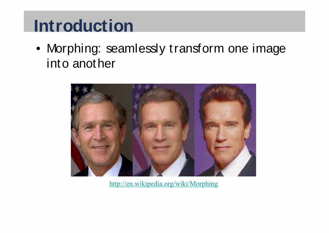
„Quality“ triangulation• Let α(T) = (α1, α2 ,.., αn) be the vector of angles

in the triangulation T in increasing orderg g

• Triangulation T1 is “better” than T2 if α(T1) > α(T2) lexicographicallyα(T2) lexicographically

• The Delaunay triangulation is the “best”http://en.wikipedia.org/wiki/Delaunay_triangulation

– Maximizes smallest angles

Good Bad

Improving a triangulation• In any convex quadrangle, an edge flip is

possiblepossible

• If this flip improves the triangulation p p glocally, it also improves the global triangulationtriangulation

Edge flipEdge flip

Naïve Delaunay algorithm• Start with arbitrary triangulation

• Flip any illegal edge until no more exist

...

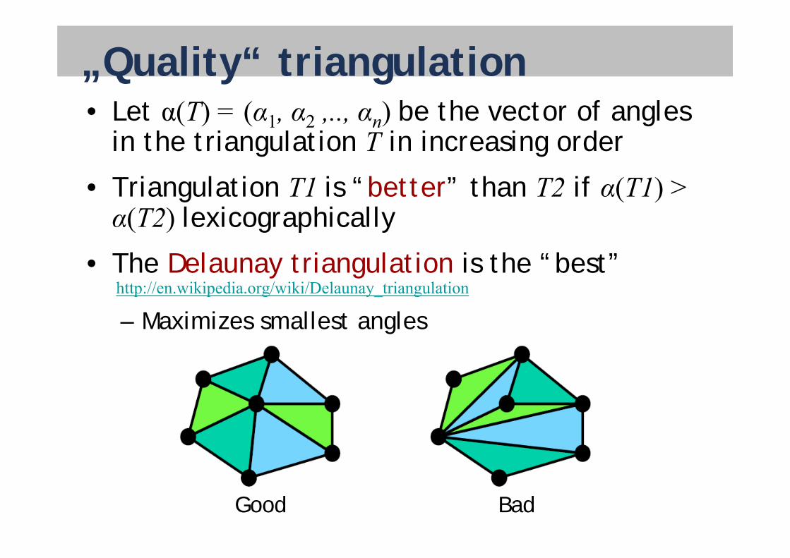
Piecewise affine mapping• Pair of corresponding triangles defines

affine mappingaffine mapping

13

2 1

3 2

Affine mappingSource Destination

Affine mapping

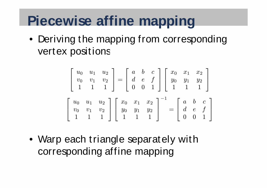
Piecewise affine mapping• Deriving the mapping from corresponding

vertex positionsvertex positions⎡u0 u1 u2

⎤ ⎡a b c

⎤⎡x0 x1 x2

⎤⎡⎣ u0 u1 u2v0 v1 v21 1 1

⎤⎦ =⎡⎣ a b cd e f0 0 1

⎤⎦⎡⎣ x0 x1 x2y0 y1 y21 1 1

⎤⎦⎡⎣ u0 u1 u2v0 v1 v21 1 1

⎤⎦⎡⎣ x0 x1 x2y0 y1 y21 1 1

⎤⎦−1 =⎡⎣ a b cd e f0 0 1

⎤⎦

W h t i l t l ith

⎣1 1 1

⎦⎣1 1 1

⎦ ⎣0 0 1

⎦

• Warp each triangle separately with corresponding affine mapping

ImplementationForward warp• For each pixel in input• For each pixel in input

imageCopy color to warped – Copy color to warped location in output

• Problem: gapsProblem: gapsInverse warp• For each pixel in output

image– Lookup color from

inverse warped location in inputin input

Source Destination

Implementation• Forward transformation

⎡⎣ u0 u1 u2v0 v1 v21 1 1

⎤⎦⎡⎣ x0 x1 x2y0 y1 y21 1 1

⎤⎦−1 =⎡⎣ a b cd e f0 0 1

⎤⎦⎣1 1 1

⎦⎣1 1 1

⎦ ⎣0 0 1

⎦

• Inverse transformation⎡x0 x1 x2

⎤⎡u0 u1 u2

⎤−1 ⎡a b cd f

⎤−1⎡⎣ y0 y1 y21 1 1

⎤⎦⎡⎣ v0 v1 v21 1 1

⎤⎦ =

⎡⎣ d e f0 0 1

⎤⎦

Implementation• Need to figure out which inverse

transformation needs to be applied to ppdestination pixel– Each triangle has different transformation– Each triangle has different transformation

• Determine in which triangle destination pixel lieslies– Need consistently oriented

t i l ( t l k i )

12

triangle (say counterclockwise)– Define edge normals

Ch k if i t i i id– Check if point is on insideof each edge using dot product

Normal

3productDestination triangle

3

Discussion• Piecewise linear warping is only C0 continuous

Fi t d i ti i t ti– First derivative is not continuous

• Not guaranteed to be one-to-one• Not guaranteed to be one to one

– Foldovers

Discussion• Many more sophisticated warping methods exist

Cage based (no mesh required)Cage-based (no mesh required)http://www.cs.technion.ac.il/~weber/Publications/Complex-Coordinates/index.html

Splines (Photoshop)Splines (Photoshop)Moving least squares interpolation

http://faculty.cs.tamu.edu/schaefer/research/mls.pdf


• Introduction

Warping• Warping


• Resampling

Morphing• Goal: smooth transition between source

and destination imageand destination image

• Separate shape and colorp p

Source Destination

Morphing• Warp each image separately, then cross-dissolve

Warp to inbetween shape Warp to inbetween shapep p Warp to inbetween shape

Morphing• Warp each image separately, then cross-dissolve

Cross-dissolve

Warp Warpp Warp

Shape interpolation• Instead of applying warp in one step, interpolate

to inbetween position

• Simplest solution: per triangle linear interpolation

(x, y) (u, v)

⎡ ⎤ ⎡ ⎤Source (t=0) Destination (t=1)

⎡⎣ xy

⎤⎦ (1− t) +⎡⎣ uv

⎤⎦ t

Note• Affine source-to-target mapping⎡

u⎤ ⎡

a b c⎤⎡

x⎤

Interpolated⎡ ⎤ ⎡ ⎤

⎡⎣ v1

⎤⎦ =⎡⎣ d e f0 0 1

⎤⎦⎡⎣ y1

⎤⎦• Interpolated

point

⎡⎣ xy

⎤⎦ (1− t) +⎡⎣ uv

⎤⎦ t

• Substitute inaffine mapping

⎡⎢⎢⎢⎣xy

1

⎤⎥⎥⎥⎦ (1− t) +⎡⎢⎢⎢⎣a b cd e f

0 0 1

⎤⎥⎥⎥⎦⎡⎢⎢⎢⎣xy

1

⎤⎥⎥⎥⎦ t =affine mapping ⎣1⎦ ⎣

0 0 1⎦ ⎣1⎦

⎛⎜⎡⎢ 1 0 00 1 0

⎤⎥(1 t) +

⎡⎢ a b cd f

⎤⎥t

⎞⎟ ⎡⎢ x ⎤⎥⎜⎜⎜⎝⎢⎢⎢⎣ 0 1 0

0 0 1

⎥⎥⎥⎦ (1− t) + ⎢⎢⎢⎣ d e f

0 0 1

⎥⎥⎥⎦ t⎟⎟⎟⎠ ⎢⎢⎢⎣ y1

⎥⎥⎥⎦• Can switch order of affine mapping and

interpolation!

Implementation• Given pair of source and

destination triangles derive

⎡⎣ a b cd e f

⎤⎦destination triangles, derive affine mapping

⎣0 0 1

⎦

• Compute interpolatedmapping

⎡⎢⎢⎢⎣1 0 00 1 00 0 1

⎤⎥⎥⎥⎦ (1− t) +⎡⎢⎢⎢⎣a b cd e f

0 0 1

⎤⎥⎥⎥⎦ tmapping

• Obtain inverse

⎣0 0 1

⎦ ⎣0 0 1

⎦⎛⎡1 0 0

⎤ ⎡a b c

⎤ ⎞−1⎛⎜⎜⎜⎝⎡⎢⎢⎢⎣ 0 1 0

0 0 1

⎤⎥⎥⎥⎦ (1− t) +⎡⎢⎢⎢⎣ d e f

0 0 1

⎤⎥⎥⎥⎦ t⎞⎟⎟⎟⎠

• Inversely map pixel in intermediate image to source imageto source image

Shape interpolation• Linear interpolation often leads to undesired

effects• Various improvements possible

E g As rigid as possible shape interpolation“– E.g., „As-rigid-as-possible shape interpolationhttp://www.cs.tau.ac.il/~dcor/online_papers/papers/arap.pdf

Triangulations

Linear

As-rigid-as-As-rigid-as-possible

Cross-dissolve• Interpolate colors linearly per-pixel

• Treat RGB color channels independently

C = I0(1 t) + I1tC = I0(1− t) + I1t

Interpolated warp, Interpolated warp,Per-pixel colorp p,Image I0

p p,Image I1

pinterpolation C

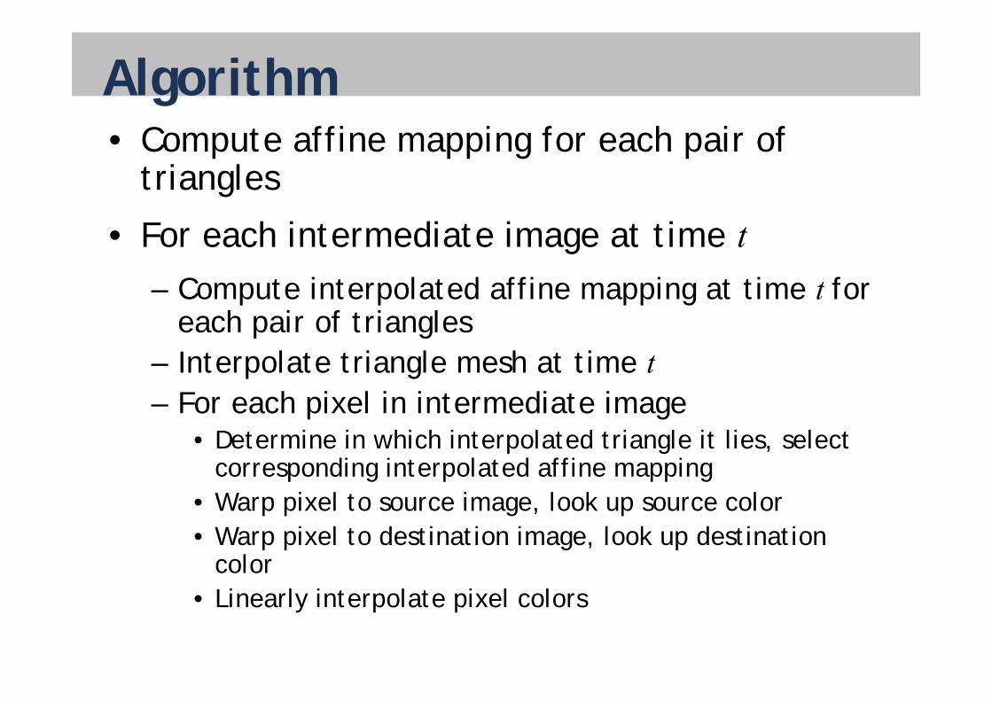
Algorithm• Compute affine mapping for each pair of

trianglesg

• For each intermediate image at time t– Compute interpolated affine mapping at time t for

each pair of trianglesl i l h i – Interpolate triangle mesh at time t

– For each pixel in intermediate imageD i i hi h i l d i l i li l • Determine in which interpolated triangle it lies, select corresponding interpolated affine mapping

• Warp pixel to source image, look up source colorWarp pixel to source image, look up source color• Warp pixel to destination image, look up destination

colorLi l i l i l l• Linearly interpolate pixel colors

Examples• http://youtube.com/watch?v=nUDIoN-_Hxs

• http://www.youtube.com/watch?gl=DE&hl=de&v=HdmnZyXAxWky

• http://www.youtube.com/watch?v=tyBs6-cmFvQ


• Introduction

Warping• Warping


• Resampling

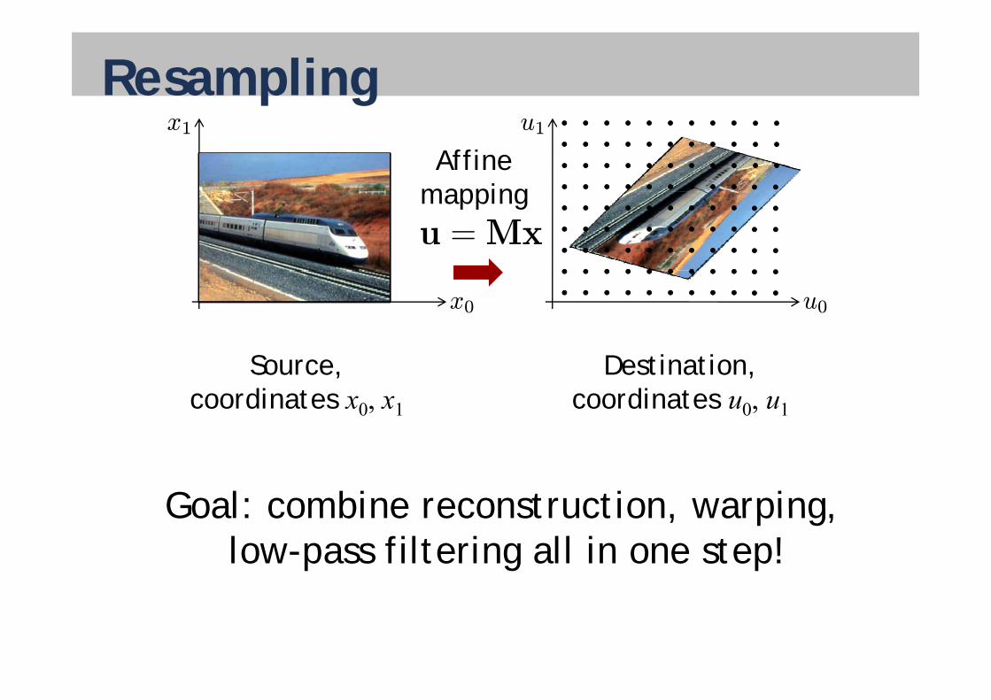
Resampling• Warped pixel location will not coincide

with source pixelswith source pixels

• Resampling: looking up and interpolating p g g p p gsource pixels

Ch ll id if– Challenge: avoid artifacts

• Great background materialghttp://www-2.cs.cmu.edu/~ph/texfund/texfund.pdf

– Image warping and texture mappingg p g pp g

Color look-up• Given warped pixel

• Closest four source pixels are at

• How to compute color of pixel?How to compute color of pixel?

Nearest-neighbor interpolation• Use color of closest source pixel

• Simple, but low quality

Bilinear interpolation1. Linear interpolation

horizontallyhorizontally

Bilinear interpolation1. Linear interpolation

horizontallyhorizontally

2. Linear interpolation vertically

Problems• In magnified regions,

not smooth enoughnot smooth enough

• In minified regions, g ,aliasing

• Goal

– In magnified regions – In magnified regions, smooth interpolationIn minified regions – In minified regions, take the average

Aliasing

P ti t f i Ph t hPerspective transform in Photoshop

ResamplingSource space Destination space

Resampling [Heckbert]http://www-2.cs.cmu.edu/~ph/texfund/texfund.pdf

Discrete input Discrete outputDiscrete input Discrete output

Reconstruct SampleLow-pass

Warp

Low passfilter

Reconstructed input Warped input Continuous output

Resamplingx1 u1

Affinemappingmappingu =Mx

x0 u0

Source,coordinates x0, x1

Destination,coordinates u0, u1

Goal: combine reconstruction warping Goal: combine reconstruction, warping, low-pass filtering all in one step!

Resamplingx1

ri(x)

x0

R t tiXfiri(x)

Reconstruction

Resamplingx1 u1

Affinemapping

ri(x)ri(M

−1u)

mappingu =Mx

x0 u0

R t ti

Xf (M 1 )

Xfiri(x) u =Mx

ReconstructionAffine mappingXfiri(M

−1u)

Resamplingx1 u1

Affinemapping

ri(x)ri(M

−1u)

mappingh(u)u =Mx

x0 u0

R t ti

Xf (M 1 )

Xfiri(x) u =Mx

ReconstructionAffine mappingXfiri(M

−1u)

Low-pass filteringXfiri(M

−1u) ? h(u) =Xfiρi

ow pass lte g

Resampling filterρi(u) = ri(M

−1u) ? h(u)Resampling filter

Resamplingx1 u1

Affinemapping

ri(x)ri(M

−1u)

mappingu =Mx h(u)

x0 u0

Source space formulation„Convolution of reconstruction

fil d d l

Destination space formulation„Convolution of warped

i fil d lfilter and warped low-pass filter in source space“

reconstruction filter and low-pass filter in destination space“

ρ0i(x) = ri(x) ? h0(x) ρi(u) = ri(M

−1u) ? h(u)

h0(x) = h(Mx)|M|where

Resamplingx1 u1

Affinemapping

ri(x)ri(M

−1u)

mappingu =Mx h(u)

x0 u0

Resampled image at destination pixel uXfiρ

0i(M

−1u)Xfiρi(M u)

Algorithm • For all destination pixels at positions u

• Map back to position in source image• Sum up contributions of all source space resampling

M−1u• Sum up contributions of all source space resampling

filters i

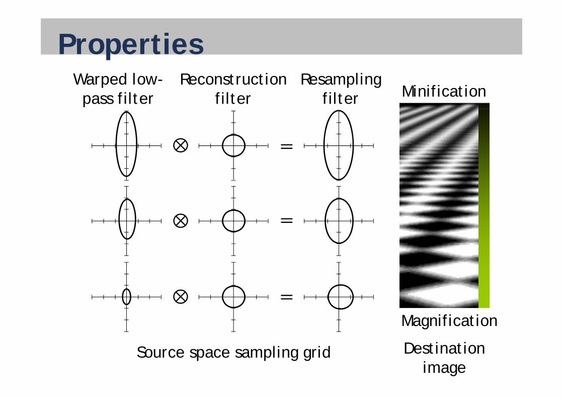
PropertiesWarped low-pass filter

Reconstructionfilter

Resamplingfilter Minification

Magnification

Source space sampling grid Destinationimage

Gaussian resampling filters• General (elliptical) 2D Gaussian

http://en.wikipedia.org/wiki/Gaussian_function#Two-dimensional_Gaussian_function

– Covariance matrix V– Centered at cCentered at c

1

2q|V|e

− 12 (x−c)TV−1(x−c)

• Convenient because

2πq|V|

• Convenient because

– Affine mapping of an (elliptical) Gaussian filter is again an Gaussian filter

– Convolution of two Gaussians is again a Gaussian– Combined resampling filter is Gaussian

Gaussian filters• Source space reconstruction filter

( )1 −1

2 (x−xi)T (x−xi)

• Destination space low-pass filter

ri(x) =2πe 2 (x xi) (x xi)

p p

h(u) =1

2πe−

12u

Tu

• Warped low-pass filter

h0(x) h(Mx)|M| |M|e−

12x

TMTMx

• Source space resampling filter

h (x) = h(Mx)|M| =2πe 2

1

D il ( h f li h l diff i )

ri(x)?h0(x) =

1

2πq|M−1M−1T + I|

e−12 (x−xi)T (M−1M−1T+I)−1(x−xi)

• Details (watch out for slightly different notation)http://www-2.cs.cmu.edu/~ph/texfund/texfund.pdf

Gaussian filters• Map destination pixel back to source

• Compute Gaussian resampling filter

Compute bounding box• Compute bounding box

• Evaluate at each source pixel in bounding Evaluate at each source pixel in bounding box, weight pixel color, sum up

M−1uM u

Bounding box• Isocontour of Gaussian is given by

r2(x) = xTVx = c• Axis aligned bounding box goes through points

on isocontour where partial derivatives vanish

r (x) = x Vx = c

on isocontour where partial derivatives vanish

∂ 2( )∂r2(x)

∂x0= 0x1

r2(x) = c

∂r2(x)

∂= 0

x0

∂x1

Bounding box• Quadratic form

2( ) TV V

⎡A B

⎤r2(x) = xTVx = c V =

⎡⎣B C

⎤⎦2( ) A 2 C 2

• Partial derivativesr2(x0, x1) = Ax

20 + 2Bx0x1 + Cx

21 = c (#)

Partial derivatives∂r2(x)

∂x= 2Ax0 + 2Bx1 = 0⇒ x0 = −B/Ax1

∂x0∂r2(x)

= 2Cx1 + 2Bx0 = 0⇒ x0 = −C/Bx1∂x1

2Cx1 + 2Bx0 0⇒ x0 C/Bx1

• Substitute for x0 in (#) and solve for x0, x1

Notes• If mapping is not affine, use local affine

approximation at each destination pixelapproximation at each destination pixel

• Tweak filter parameters for visually best p yresults

• Can use radial filter profiles other than exponential (Gaussian filter)p ( )

Notes• Anisotropic texture filtering in computer

graphics often implemented as approximation graphics often implemented as approximation to procedure described herehttp://en.wikipedia.org/wiki/Anisotropic_filtering

Trilinear mipmapping Anisotropic filtering

Next time• Panoramas

Matthias Zwicker University of Bern Fall...

Documents

Transcript of Matthias Zwicker University of Bern Fall...