Stat 251 Paper Review:

“A Jump Diffusion Model for Option Pricing,”

S. G. Kou

Matthew Pollard∗

11th May 2006

Abstract

This paper surveys the family of Jump Diffusion (JD) models for price variation.

It focuses on the Double Exponential Jump Diffusion (DEJD) model proposed by

Kou (2002). This simple model has several nice features allowing for analytic pric-

ing solutions for many options, notably exotic and path-dependent. The features

and specification of the DEJD model are discussed and placed into the general

framework of Affine Jump Diffusion models proposed by Duffie (1995). The ap-

proximate returns distribution is derived and compared with the normal. It looks

at equilibrium conditions imposed on jump diffusions under the rational expec-

tations model. Simulations of the DEJD model are presented and compared to

the S&P 500 index. Empirical testing and estimation of the model parameters is

discussed.

1 Introduction

Almost every aspect of modern finance, from valuations and portfolio choice to op-tion pricing and corporate finance, critically depend on the distribution describing thedynamics of security prices. For nearly a century, this distribution was normal. TheBrownian motion model, first proposed in Bachlier’s thesis Theorie de la Speculation(1900) and the geometric Brownian motion model (GBM) first proposed by Osborne(1959), have been enshrined in Finance’s two most successful theories: the Capital As-set Pricing Model (Sharpe, 1964) and the Black-Scholes Model (Black and Scholes, 1972)

Despite the success of the Black-Scholes model, empirical evidence against GBM hasaccumulated; see, among others, Sundaresan, 2000. Specifically, (1) real returns are notnormally distributed, instead the tails are asymmetric and heavier than normal (called“leptokurtotic”) , (2) volatility is not constant, instead it clusters into high and lowlevels and displays long range dependence, (3) a “volatility smile” in calculating impliedvolatilies through the Black-Scholes framework exists, see Bakashi et al. (1997) for anoverview.

∗Department of Statistics, University of California Berkeley; matthewcpollard@berkeley.edu

1

The inadequacy of Brownian motion has led to development of many alternativecontinuous-time models for price variation. These include stochastic volatility models,see Duffie (1995); conditional heteroskedastic models, in particular ARCH (Engle, 1982)and GARCH (Bollerslev, 1986); a chaos theory, multi-fractal model, see Mandelbrot(1963); and jump-diffusion models (JD), see Merton (1976a) and Kou (2002).

The jump-diffusion model was first suggested by Merton (1976a, 1976b), followingthe work of Press (1967). Merton suggested that returns processes consist of threecomponents, a linear drift, a Brownian motion representing “normal” price variations,and a compound Poisson process accounting for “abnormal” changes in prices (jumps)generated by important information arrivals. Upon each information arrival, the jumpmagnitude is determined by sampling from an independent and identically distributed(i.i.d) random variable.

A large class of JD models have been proposed; see Duffie (1995) and Merton (1990)for reviews. Merton’s first 1976 model assumes that this distribution is log-normallydistributed (LND), which renders estimation and hypothesis testing tractable. It has alsobeen shown to be consistent with empirical return distributions, displaying higher peaks,excess kurtosis and skewness; see Bakshi, Cao & Chen, 1997. However, analytic pricingformulas for only very simple options, such as European and American, exist underthis distribution (Kou, 2002). Proposed variations on Merton’s model include differentdistributional assumptions for jump magnitude (Ramezani & Zeng, 1998; Andersen &Andereasen, 2000; Kou, 2002), time-varying jump intensity, correlated jump-size (Naik(1993) and models where both price and volatility jump (Bakshi & Cao, 2004 and Erakeret al., 2003).

Each of these specific formulations are special cases of the Affine Jump Diffusion(AJD) framework proposed by Duffie, Pan and Singleton (2000). This framework ispopular among researchers due to its modelling flexibility and its tractability in de-riving risk-neutral representations for options pricing, as well as for straight-forwardeconometric estimation.

The Double Exponential Jump Diffusion (DEJD) model proposed by Kou (2002)is a special case of the AJD family. The model model enjoys several nice properties.The returns implied by the model are leptokurtotic and asymmetric. The model fitsobserved volatility smiles well. The model can be embedded into a rational expectionsequilibrium framework. Most importantly, the memoryless property of the exponentialdistribution family allows pricing formulas for exotic and path-dependent to be obtainedexactly. This is a significant advantage over alternative JD models in which analytictractability is confined to plain vanilla options. Because of these features, the DEJD isa popular choice within the JD family and has been used to model price variation instock indices (Ramezani & Zeng, 2004) and bond yield spread (Huang & Huang, 2003).

The remainder of this paper considers the DEJD model in detail. It summarizes themain results of Kou (2002), the returns distribution under jumps, that DEJD can beembedded into a rational expectations equilibrium framework, and pricing formulas forEuropean options. No empirical work was carried out to test the DEJD in Kou’s study.I look at the work of Ramexani and Zeng (2004), which empirically assesses the DEJDmodel against LJD and ARCH alternative models. This is the only empirical study to

2

date to consider the DEJD model. They conclude the results are, at best, weak.The paper is structured as follows. Section 2 presents the Merton and the Double

Exponential Jump Diffusion models. A simulation is carried out to graphically comparethe returns distribution under DEJD to GBM and real returns from the S&P-500 in-dex. Section 3 solves the DEJD stochastic differential equation and, from this solution,derives approximations to the returns density. It presents Kou’s exact density result,and provides an illustrative example comparing the DEJD returns density to GBM re-turns density. Section 4 briefly looks at general equilibrium theory and the rationalexpectations model (Lucas, 1978), and considers the result the log of the jump distribu-tion must belong in the exponential family. Section 5 discusses the problems of marketincompleteness under jump-diffusions and existence of risk-free measures, and derivesthe discounted payoff expectation equal to the price of a European call option. Kou’sformula for evaluating this expectation is given. Finally, section 6 surveys the empiri-cal work done in assessing the DEJD model compared to other JD models and ARCHspecifications.

2 The Jump-Diffusion Model

2.1 Merton’s Model

The jump-diffusion model on which Kou’s model is based was described by Merton(1976), which we follow here. The model for price variation consists of two parts:(1) a continuous diffusion according to geometric Brownian motion and (2) randomtime discontinuous jumps. The economic reasoning behind adding jumps is that thesecorrespond to important information revelations that cause the market to quickly revaluethe underlying asset. Under Merton’s model, the jump process is specified by a Poissonprocess with intensity λ, thus

P (jump in [t + ∆t)) = λ∆t + o(∆t).

and the times between jumps are i.i.d exponential random variables. Upon the ith eventtime, the jump magnitude Yi is drawn i.i.d from the log-normal distribution and theprice changes from St to StYi. Merton notes that under the log-normal assumption, thedistribution of St/So is lognormal with random variance parameter following the Poissondistribution.

2.2 Double Exponential Jump Diffusion Model

Kou proposes simple jump-diffusion model where the price of a financial asset is mod-elled by two parts, continuous geometric Brownian motion and jumps at random timeswith logarithm of jump sizes having double exponential distribution. The DEJD modelhas several nice features compared to alternative JD models. The returns distributionare asymmetric and leptokurtotic. Kou shows that the “volatility smile” exists undersimulated prices with double exponential jumps. Most importantly, the model has goodanalytic tractability.

3

Specifically, under the DEJD model, the price of an underlying asset, St, is assumedto satisfy the stochastic differential equation

dSt

St= µdt + σdWt + d

N(t)∑i=1

(Vi − 1)

v (1)

where Wt is a standard Brownian motion, N(t) is a Poisson process with rate λ and {Vi}is a sequence of independent and identically distributed nonnegative random jump sizes.The µdt + σdWt specifies a continuous geometric Brownian motion with instantaneousµ drift and σ volatility. The random increment d

∑N(t)i=1 (Vi−1) produces a jump (Vi−1)

during time t ∈ [s, s + ds] upon the event N(s + ds) = 1 + N(s).The distribution of Y = log(V ) is asymmetric double exponential with density

fY (y) = pη1e−η1y1{y≥0} + qη2e

η2y1{y<0}, η1 > 0, η2 > 0 (2)

where p, q ≥ 0 and p+ q = 1, represent the probability of upward and downward jumps.This is equivalently,

Y =

{ξ+, with probability p

−ξ−, with probability q,

where ξ+ and ξ− are exponential random variables with rates η1 and η2 respectively.This distribution was first proposed by Laplace (1774), giving rise to another name –“the first law of Laplace”, whereas the “second law of Laplace” is the normal density.The processes Wt, N(t), and Vi are assumed to be independent. Some useful propertiesof Y and V are

E(Y ) =p

η1− q

η2, Var(Y ) = pq(

1η1− 1

η2)2 + (

p

η21

+q

η22

),

E(V ) = E(eY ) = qη2

η1 + 1+ p

η1

η1 − 1, η1 > 1, η2 > 0.

Example Consider figure (1), which shows three series of plots: the log prices andreturns of the S&P 500 index from 1950 to 2006, log prices and returns generatedby the DEJD model. The simulated returns from DEJD are generated by discreteapproximation of the SDE, see Pollard (2006a) for details, and R code to do this ispresented in A.2 of the Appendix.

The parameters for the DEJ with µ = 20% per annum, σ = 20% per annum, ∆t = 1day, λ = 20, κ = −0.02 and η = 0.02. That is, I assume that there are about 20 dailyjumps per year with average jump size −2% and with jump volatility 2%.

It is clear that GBM returns bear little resemblance to real returns – to recentlyquote Mandelbrot, “nothing happens” in GBM. The DEJD model seems to performconsiderably better. The real returns experience occasional large jumps, such as October1987’s Black Tuesday, and the DEJD model captures. However, close inspection of realreturns reveals that the volatility of “normal” variation oscillates between high and lowslowly between years. The DEJD is not capturing this additional dynamic in prices

4

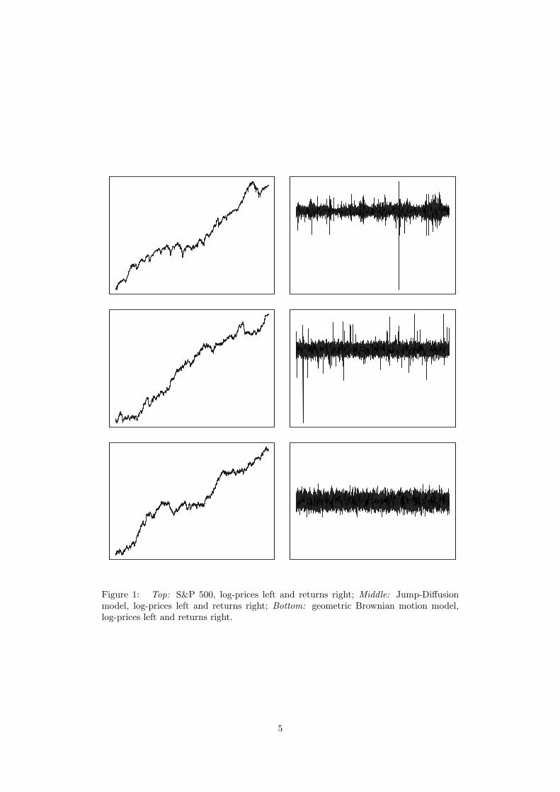
Figure 1: Top: S&P 500, log-prices left and returns right; Middle: Jump-Diffusionmodel, log-prices left and returns right; Bottom: geometric Brownian motion model,log-prices left and returns right.

5

variation.

3 Return Distribution

The solution to the stochastic differential equation in equation (1) is given by

St = S0exp{(µ− 12σ2)t + σWt}

N(t)∏i=1

Vi. (3)

This result generalizes the solution for GBM, St = S0exp{(µ− 12σ2)t+σWt}, to include

stochastic jumps. Proof of (3) is given in A.1 of the Appendix. From (3) , the simplereturn of the underlying asset in a small time increment ∆t becomes

St+∆t − St

St= exp

(µ− σ2/2)∆t + σ(Wt+∆t −Wt) +N(t+∆t)∑i=N(t)+1

Yi

− 1

where Xi = log(Vi). For small ∆t, we have the approximation ex ≈ 1 + x + x2/2 andthe result (∆Wt)2 ≈ ∆t to obtain

St+∆t − St

St≈ (µ− σ2/2)∆t + σ∆Wt +

N(t+∆t)∑i=N(t)+1

Xi +12σ2(∆Wt)2

≈ µ∆t + σZ√

∆t +N(t+∆t)∑i=N(t)+1

Xi,

where Z is a random variable with standard normal distribution and ∆Wt = Wt+∆t−Wt.

Under the assumption N(t) follows a Poisson process, the probability of having onejump in the interval (t, t+∆t] is λ∆t and having more than one is o(∆t). Therefore, forsmall ∆t, we have

N(t+∆t)∑i=N(t)+1

Xi ≈

{XN(t)+1 with probability λ∆t

0 with probability 1− λ∆t

and combining these results, the simple return of the underlying asset is approximatelydistributed as

St+∆t − St

St≈ µ∆t + σZ

√∆t + I ×X, (4)

where I is a Bernoulli random variable with P (I = 1) = λ∆t. Equation (4) allowsfor simple simulation of the returns generated by the DEJD model. Simulations arepresented in figure (1), discussed in Section 7. The function used to simulate returnsand code is presented in A.2 of the Appendix.

Let G equal the right hand side of (4). Using the independence between the expo-nential and normal distributions used in the model and formulae for the sum of doubleexponential random variables, Kou (2002) obtains the probability density function of G

6

−10 −5 0 5 10

0.00

0.05

0.10

0.15

0.20

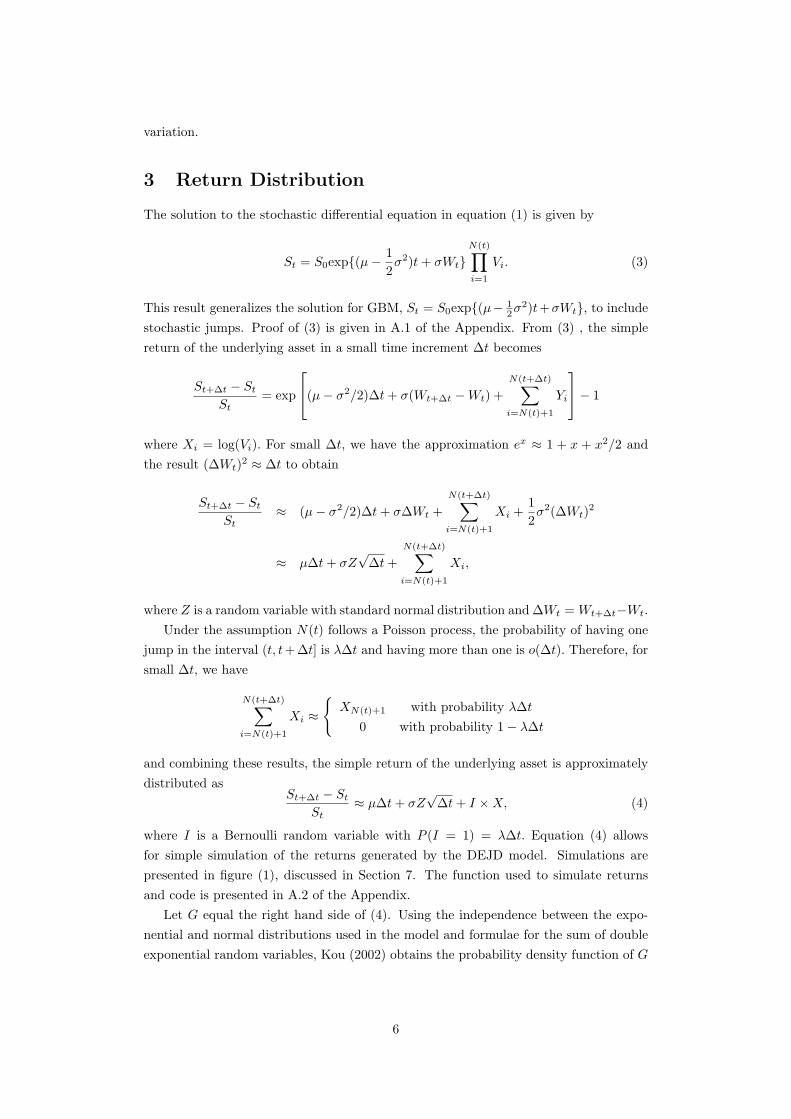
Figure 2: Density g(x) for a double exponential (red) with µ = 0.1, λ = 1,∆t = 1κ = 0.1, and density of normal (black, broken) with equal mean and variance.

as

g(x) =λ∆t

2ηeσ2∆t/(2η2)

{e−ω/ηΦ

(ωη − µ∆t

ση√

∆t

)+ eω/ηΦ

(ωη + µ∆t

ση√

∆t

)}+(1− λ∆t)

1σ√

∆tf

(x− µ∆t

σ√

∆t

),

where ω = x − µ∆t − κ, and f(.) and Φ(.) are the probability density and cumulativedistribution functions of the standard normal random variable. The density g has meanand variance given by

E(G) = µ∆t + λ∆tκ

V ar(G) = σ2∆t + 2η2λ∆t + κ2λ∆t(1− λ∆t).

The density g(x), comparing to a normal density with equal mean and variance, has ahigher peak and two heavy tails. The distribution is not symmetric: if the mean jumpsize κ > 0, the distribution is skewed right; and if κ < 0, skewed left. An example ofg(x) with parameters µ = 0.1, λ = 1,∆t = 1 κ = 0.1 is drawn in figure (2) with a normaldensity overlayed.

4 Equilibrium under Jump Diffusion

The prices of any asset, financial or otherwise, is subject to forces of demand and supply.By guidance of the market’s “invisible hand”, the adjustment of prices brings these forcesto equality. The point where demand and supply match, the equilibrium point, needsto exist, be unique and determinable if asset prices, such as options prices, are to bepredictable from theory.

Economists classify market equilibrium models into two categories, partial and gen-

7

eral Partial equilibrium models take the variables of prices, expectations and preferencesas given, and derive results that are assumed not to affect these market variables. Op-tion pricing models are typically partial equilibrium models, and a famous example isthe Black-Scholes model. Here, the expected return of a security, the risk free inter-est rate and the volatility are all determined independently of the model, and investorpreferences do not matter.

General Equilibrium models provide results by aggregating across assets and marketparticipants. They take the existence of a class of assets, the prices of those assets,and the expectations and preferences of all market participants as variables that aredetermined by the model itself. The simplest general equilibrium model is called theRational Expectations model (Lucas, 1978) and forms the basis of the Efficient MarketHypothesis.

Kou considers the family of jump diffusion models and whether a market equilibriumexists under rational expectations model. Under this model, there is only one risky assetwith price p(t). People (“agents”) are homogeneous and each try to solve the utilitymaximization problem

maxc

E

[∫ ∞

0

U(c(t), t)dt

]where U(c(t), t) is the utility function of the consumption process c(t). Each agent has anexogenous endowment process, δ(t), which provides income that can be either consumedor invested in a single risky asset that pays no dividends. If δ is Markovian, Stokey andLukas (1989) show that under mild conditions, p(t) must satisfy the Euler equation

p(t) =E[Uc(δ(T ), T )p(T )|Ft]

Uc[δ(t), t], ∀T ≥ t ≥ 0, (5)

where Uc is the marginal utility of consumption at time t.Kou explicitly derives the implication of equation (5) when the endowment process

δ(t) and the price St of the underlying asset are stochastic and satisfies the jump-diffusionSDE in (1) with jumps (Vi − 1) with Vi having arbitrary distribution. Specifically, heproposes a special correlated jump diffusion form for S(t),

dSt

St= µdt + σ(ρdW 1

t +√

1− ρ2dW 2t }+ d

N(t)∑i=1

(Vi − 1)

, Vi = Vi

β(6)

where the power β ∈ (−∞,∞) is an arbitrary constant, where W 1t is independent of W 2

t

and W 1t drives the jump diffusion for δ(t) given by (1). He considers equilibrium only

under special utility function forms

U(c, t) =e−θtcα

α, 0 < α < 1, U(c, t) = e−θtlog(c), if α = 0.

Kou’s first theorem states that the model in (6) satisfies the equilibrium conditions ifand only if

µ = r + σ1σ2ρ(1− α)− λ(ϕ(α+β−1)1 − ϕ

(α−1)1 )

8

where ϕ(a)1 := E[(V a

i −1)], the expected proportional jump size affecting the endowmentδ(t).

The second important result specifies possible distributions the endowment jump, V

. Let V be the family distributions for V . Then if for any real number a,

V a ∈ V, kxafV

(x) ∈ V

where k = {ϕ(a−1)1 + 1}−1,then the jump sizes for the asset price St under the phys-

ical probability measure P and jump sizes for St under the rational expectation risk-neutral measure Q belong to the same family V. Kou notes that this essentially requiresY = log(V ) to belong to the exponential distribution family. This condition satisfiedboth with Y having normal distribution, as in the LJD model, and Y having doubleexponential distribution.

5 Option Pricing

A serious criticism of JD models is that under the presence of random jumps the marketbecomes incomplete. This mean that replication of an option, or equivalently, risklesshedging of an option position, is impossible since prices discontinuously jump. However,Kou argues that this should be considered only as a special property of the BrownianMotion framework, and since riskless hedging is impossible in discrete time, this lossshould not make a difference to the actual value of an option. This is also voiced byMerton (1976a) and Naik and Lee (1990).

Given incompleteness, we can still derive option pricing formula that does not dependon risk attitudes of investors. Merton (1976a) proposes an economic argument: that, ifthe number of securities available is very large, the risk of sudden jumps is diversifiableand the market will therefore pay no risk premium over the risk-free rate for bearingthis risk. Alternatively, for a given set of risk premiums, we can consider a risk-neutralmeasure Q so that under Q

dSt

St= [r − λϕ]dt + σdWt + d

N(t)∑i=1

(Vi − 1)

where r is the risk-free interest rate, σ is price volatility between jumps, λ is jumpintensity,

ϕ = E[V − 1] = exp(κ)/(1− η2)− 1

where κ = E(Y ), and the parameters r, σ, λ, κ and η become risk-neutral parameterstaking consideration of the risk premiums. Kou constructs Q under the rational expec-tations framework as follows. Let δ(t) be a stochastic endowment process satisfying theDEJD SDE as before, and define

Z(t) := ertUc(δ(t), t) = e(r−θ)t(δ(t))α−1

where θ and α are parameters in investor’s intertemportal consumption utility function.

9

Then Z(t) is a martingale under P , and define the measure Q by the Radon-Nikodymderivative

dQ

dP:=

Z(t)Z(0)

.

Then under Q, the Euler equation (5) holds if and only if

St = e−r(T−t)EQ(ST |Ft).

The unique solution of this SDE is

St = S0exp[(r − σ2/2− λϕ)t + σdWt]N(t)∏i=1

Vi,

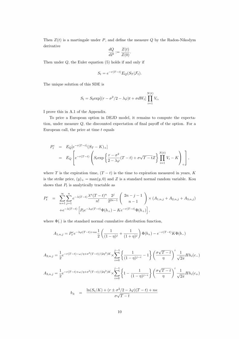
I prove this in A.1 of the Appendix.To price a European option in DEJD model, it remains to compute the expecta-

tion, under measure Q, the discounted expectation of final payoff of the option. For aEuropean call, the price at time t equals

P ct = EQ[e−r(T−t)(ST −K)+]

= EQ

e−r(T−t)

Stexp{

r − σ2

2− λϕ(T − t) + σ

√T − tZ

}N(t)∏i=1

Vi −K

+

,

where T is the expiration time, (T − t) is the time to expiration measured in years, K

is the strike price, (y)+ = max(y, 0) and Z is a standard normal random variable. Koushows that Pt is analytically tractable as

P ct =

∞∑n=1

n∑j=1

e−λ(T−t) λn(T − t)n

n!2j

22n−1

(2n− j − 1

n− 1

)× (A1,n,j + A2,n,j + A3,n,j)

+e−λ(T−t)[Pte

−λϕ(T−t)Φ(h+)−Ke−r(T−t)Φ(h+)],

where Φ(.) is the standard normal cumulative distribution function,

A1,n,j = P ct e−λϕ(T−t)+nκ 1

2

(1

(1− η)j+

1(1 + η)j

)Φ(b+)− e−r(T−t)KΦ(b−)

A2,n,j =12e−r(T−t)−ω/η+σ2(T−t)/(2η2)K×

j−1∑i=0

{1

(1− η)j−i− 1}(

σ√

T − t

η

)i1√2π

Hhi(c−)

A3,n,j =12e−r(T−t)+ω/η+σ2(T−t)/(2η2)K×

j−1∑i=0

{1− 1

(1− η)j−i

}(σ√

T − t

η

)i1√2π

Hhi(c+)

b± =ln(St/K) + (r ± σ2/2− λϕ)(T − t) + nκ

σ√

T − t

10

h± =ln(St/K) + (r ± σ2/2− λϕ)(T − t)

σ√

T − t

c± =σ√

T − t

η± ω

σ√

T − t

ω = ln(K/Pt) + λϕ(T − t)− (r − σ2/2)(T − t)− nκ

ϕ =eκ

1− η2− 1

and the Hni(.) functions are defined by

Hnn(x) =1n!

∫ ∞

x

(s− x)ne−s2/2ds, n = 0, 1, ...

and Hh−1(x) = exp(−x2/2), which is 2πf(x) where f(x) is the probability densityfunction of the standard normal variable. The Hhn(x) functions satisfy the recursion

nHhn(x) = Hhn−2(x)− xHhn−1(x), n ≥ 1,

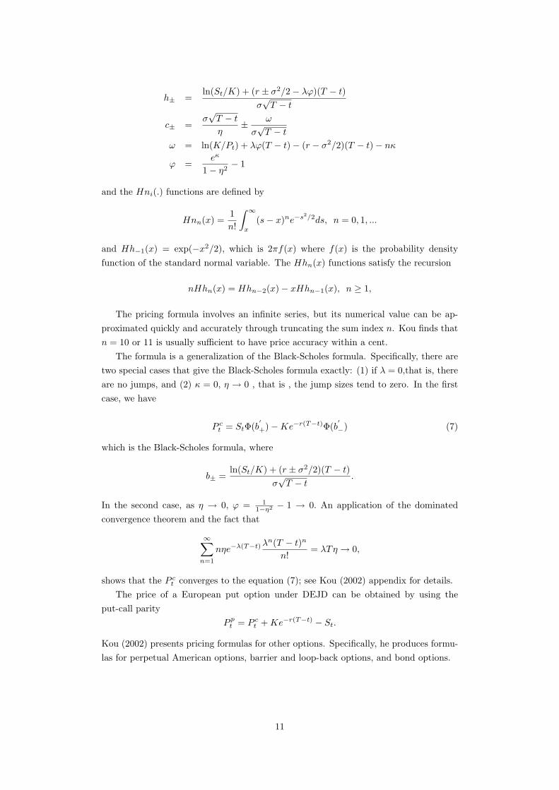
The pricing formula involves an infinite series, but its numerical value can be ap-proximated quickly and accurately through truncating the sum index n. Kou finds thatn = 10 or 11 is usually sufficient to have price accuracy within a cent.

The formula is a generalization of the Black-Scholes formula. Specifically, there aretwo special cases that give the Black-Scholes formula exactly: (1) if λ = 0,that is, thereare no jumps, and (2) κ = 0, η → 0 , that is , the jump sizes tend to zero. In the firstcase, we have

P ct = StΦ(b

′

+)−Ke−r(T−t)Φ(b′

−) (7)

which is the Black-Scholes formula, where

b± =ln(St/K) + (r ± σ2/2)(T − t)

σ√

T − t.

In the second case, as η → 0, ϕ = 11−η2 − 1 → 0. An application of the dominated

convergence theorem and the fact that

∞∑n=1

nηe−λ(T−t) λn(T − t)n

n!= λTη → 0,

shows that the P ct converges to the equation (7); see Kou (2002) appendix for details.

The price of a European put option under DEJD can be obtained by using theput-call parity

P pt = P c

t + Ke−r(T−t) − St.

Kou (2002) presents pricing formulas for other options. Specifically, he produces formu-las for perpetual American options, barrier and loop-back options, and bond options.

11

6 Empirical Assessment

In his concluding comments, Kou (2002) notes that no empirical work was carried outto test the DEJD in his study. At the time of writing, only one study, Ramexani andZeng (2004) ,has investigated the model against real data.

Ramezani and Zeng (2004) compare DEJD to six popular versions of the Autore-gressive Conditional Heteroskedasticity (ARCH) and the Log-Normal Jump Diffusion(LJD) specification. They fit each model to daily data from a large sample of firms andmonthly data from the S&P-500 and NASDAQ composite. The fit is carried out by max-imum likelihood estimation and they utilize the BIC criterion to assess the performanceof DEJD relative to the alternatives.

For individual stocks based on data spanning the period 10/96 to 12/98, they findboth LJD and DEJD fit the data better than GBM for every firm, supporting the use ofjump-diffusion models. Surprisingly, they find that that relative to LJD, DEJD providesa better fit for only 11% of the sampled firms. The results fell short of their expectations,given the flexibility associated with DEJD.

For comparison with ARCH specifications, they found that both DEJD and LJDperform better than the ARCH alternatives for the majority of individual stocks. Forstock indexes, the ARCH specifications dominate, in particular, GARCH(1,1) dominatefor monthly indexes and EGARCH(1,1) for daily indexes. The GBM specification failsto beat the alternatives for every time series.

In conclusion, they find that at best, the empirical evidence for DEJD is mixed.

7 Conclusion

This paper reviews the class of jump diffusion models paying particular focus on theDouble Exponential Jump Diffusion process proposed by Kou (2002). Under this model,the price of a financial asset is modelled by two parts, continuous geometric Brownianmotion and jumps at random times with logarithm of jump sizes having double expo-nential distribution. The DEJD model has several nice features compared to alternativeJD models. The returns distribution are asymmetric and leptokurtotic. Kou shows thatthe “volatility smile” exists under simulated prices with double exponential jumps. Mostimportantly, the model has good analytic tractability, allowing for explicit calculation ofboth vanilla and path-dependent prices. The explicit calculation is made possible partlybecause of the memoryless property of the double exponential distribution. Further-more, the model is compatible with a rational expectations framework unlike modelsusing jump distribution outside the exponential family.

However, the work by Ramezani and Zeng (2004) suggest that the DEJD modelis outperformed by Merton’s log-normal jump diffusion specification in modelling thereturns from individual stock and is dominated by GARCH(1,1) specifications for theS&P-500 and NASDAQ index. This is surprising given the flexibility of the DEJDmodel.

There are a number of interesting directions for future extensions of the model.Ramezani and Zeng (2004) suggest alternatives using time-varying jump intensities.

12

Adding correlation to the jump process may be used to simulate volatility clusteringeffects into the model. Alternatively, the plots in figure (1) suggest that a hybrid jumpand stochastic volatility model are the best approach for empirical success. Of course,it should be noted that the main reason the DEJD model is attractive is its simplicity.Its unclear whether adding further bells and whistles improves things.

A Appendix

A.1 Solving the DEJD Model

The solution the stochastic differential equation in (??) is given by

St = S0exp[(µ− σ2/2− λϕ)t + σWt]N(t)∏i=1

Vi,

where∏0

i=1 = 0. The solution is obtained as follows.Let ti be time corresponding to the ith jump. For t ∈ [0, t1), there is no jump and

the price is given by the solution to dSt/St = (r−λϕ)dt+σdWt. Consequently, the lefthand price limit at t1 is

St−1= S0exp(µ− σ2/2− λϕ)t1 + σWt1 ].

At time t1, the proportion of price jump is V1 − 1 so the price becomes

St1 = (1 + V1 − 1)Pt−1= V1Pt−1

= P0exp[(µ− σ2/2− λϕ)t1 + σWt1 ]V1.

For any t ∈ (t1, t2), there is no jump in the interval (t1, t] so that

St = St1exp[(µ− σ2/2− λϕ)(t− t1) + σ(Wt −Wt1)].

Plugging in St1 yields

St = S0exp([µ− σ2/2− λϕ)t + σWt]J1,

and repeating this scheme, we obtain the solution.

A.2 Program Code

A.2.1 rdexp

Draws random variates from the double exponential distribution specified by (2). Thecall variables are n (number of variates), p (skewness parameter, p > 0 means skewedright), and η1and η2 (rates of left and right exponential distributions).

rdexp = function(n,p,mu1,mu2) {nleft = rbinom(1,n,p)leftexp = -rexp(nleft,mu1)

13

rightexp = rexp(n-nleft,mu2)s = sample(c(leftexp,rightexp),size=n,replace=F)return(s) }

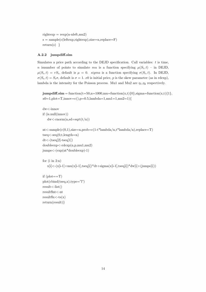
A.2.2 jumpdiff.sim

Simulates a price path according to the DEJD specification. Call variables: t is time,n isnumber of points to simulate mu is a function specifying µ(St, t) – in DEJD,µ(St, t) = rSt, default is µ = 0. sigma is a function specifying σ(St, t). In DEJD,σ(St, t) = Stσ, default is σ = 1. x0 is initial price, p is the skew parameter (as in rdexp),lambda is the intensity for the Poisson process. Mu1 and Mu2 are η1,η2 respectively.

jumpdiff.sim = function(t=50,n=1000,mu=function(x,t){0},sigma=function(x,t){1},x0=1,plot=T,innov=c(),p=0.5,lambda=1,mu1=1,mu2=1){

dw<-innovif (is.null(innov))

dw<-rnorm(n,sd=sqrt(t/n))

nt<-sample(c(0,1),size=n,prob=c(1-t*lambda/n,t*lambda/n),replace=T)tseq<-seq(0,t,length=n)dt<-(tseq[2]-tseq[1])doubleexp<-rdexp(n,p,mu1,mu2)jumps<-(exp(nt*doubleexp)-1)

for (i in 2:n)x[i]<-(x[i-1]+mu(x[i-1],tseq[i])*dt+sigma(x[i-1],tseq[i])*dw[i]+(jumps[i]))

if (plot==T)plot(cbind(tseq,x),type=”l”)result<-list()result$nt<-ntresult$x<-ts(x)return(result)}

14

References

[1] Merton, R., “Option Pricing When Underlying Stock Returns are Discontinuous”,Journal of Financial Economics, 3, 125-14, 1976.

[2] Sharpe, W., “Capital Asset Prices - A Theory of Market Equilibrium Under Con-ditions of Risk,” Journal of Finance, 425-442, 1964.

[3] Black, F., & M. Scholes.“The Pricing of Options and Corporate Liabilities.”Journalof Political Economy, 81, 637-654 , 1973.

[4] Osborne, M., “Brownian motion in the stock market,” Operations Research 7, 145-173, 1959.

[5] Sundaresan, S., “Continuous-time methods in finance: A review and an assessment,”Journal of Finance, 55, 1569-1622, 2000.

[6] Bakshi, G., Cao, C. & Chen, Z., “Empirical performance of alternative option pric-ing models,” Journal of Finance, 52, 2003-2049, 1997.

[7] Duffie, D., “Dynamic Asset Pricing Theory,” 2nd edn. Princeton University Press,Princeton, 1995.

[8] Engle, R., “ARCH, Selected Readings,” Oxford University Press, Oxford, 1995.

[9] Bollerslev, T., “Generalized Autoregressive Conditional Heteroskedasticity,” Jour-nal of Econometrics, 31, 307-327, 1986.

[10] Mandelbrot, B., “The variation of certain speculative prices”, Journal of Business,36, 394-419, 1963.

[11] Merton, R,“Option pricing when underlying stock returns are discontinuous,”, Jour-nal of Financial Economics, 3, 224-244, 1976a.

[12] Merton, R, “The impact on option pricing of specification error in the underlyingstock price returns,”, Journal of Finance, 31, 333-350, 1976b.

[13] Kou, S., “A jump diffusion model for option pricing,” Management Science 48,1086-1101, 2002.

[14] Press, J., “A Compound Events Model of Security Prices,” Journal of Business, 40,317-335, 1967.

[15] Ramezani, C. & Zeng, Y., “Maximum likelihood estimation of asymmetric jumpdiffusion processes: application to security prices.”, working paper, University ofWisconsin, Madison, 1998.

[16] Andersen, L. & Andreasen, J., “Volatility Skews and Extensions of the Libor MarketModel”, Applied Mathematical Finance, Vol 7, 1-32, 2000.

[17] Naik, V., “Option valuation and hedging strategies with jumps in the volatility ofasset returns,” Journal of Finance, 48, 1969-1984, 1993.

15

[18] Bakshi, G & Cao, C.“Disentangling the contribution of return-jumps and volatility-jumps on individual equity option prices,” working paper, Smith Business School,University of Maryland, 2004.

[19] Duffie, D., Pan, J., & Singleton, K., “Transform Analysis and Option Pricing forAffine Jump-Diffusions,” Econometrica, 68, 1343-1376, 2000.

[20] Ramezani, C., & Zeng, Y., “An Empirical Assessment of the Double ExponentialJump-Diffusion Process,” working paper, University of Missouri, 2004.

[21] Huang, J., & Huang, M., “How much of the corporate-treasury yield spread is dueto credit risk?,” working paper, Graduate School of Business, Stanford University,2003.

[22] Lucas, R., “Asset prices in an exchange economy”, Econometrica, 46, 1429-1445,1978.

[23] Naik, V., & Lee, M., “General equilibrium pricing of options on the market portfoliowith discontinuous returns,” Review of Financial Studies, 3, 493- 521, 1990.

16