Matter waves of Bose-Fermi mixtures in one-dimensional...

Matter waves of Bose-Fermi mixtures in one-dimensional optical lattices

Yu. V. Bludov,1,* J. Santhanam,2,† V. M. Kenkre,2,‡ and V. V. Konotop1,3,§

1Centro de Física Teórica e Computacional, Universidade de Lisboa, Complexo Interdisciplinar,Avenida Professor Gama Pinto 2, Lisboa 1649-003, Portugal

2Consortium of the Americas for Interdisciplinary Science and Department of Physics and Astronomy, University of New Mexico,Albuquerque, New Mexico 87131, USA

3Departamento de Física, Universidade de Lisboa, Campo Grande, Edifício C8, Piso 6, Lisboa 1749-016, Portugal�Received 10 May 2006�

We describe solitary wave excitations in a Bose-Fermi mixture loaded in a one-dimensional and stronglyelongated lattice. We focus on the mean-field theory under the condition that the fermion number significantlyexceeds the boson number, and limit our consideration to lattice amplitudes corresponding to the order of a fewrecoil energies or less. In such a case, the fermionic atoms display “metallic” behavior and are well-describedby the effective mass approximation. After classifying the relevant cases, we concentrate on gap solitons andcoupled gap solitons in the two limiting cases of large and small fermion density, respectively. In the former,the fermionic atoms are distributed almost homogeneously and thus can move freely along the lattice. In thelatter, the fermionic density becomes negligible in the potential maxima, and this leads to negligible fermioniccurrent in the linear regime.

DOI: XXXX PACS number�s�: 03.75.Lm, 03.75.Kk, 03.75.Ss

I. INTRODUCTION

It is widely recognized that optical lattices �OLs� providea powerful tool to manipulate matter waves, in particularsolitons, and to test properties emerging from the interplaybetween periodicity of the medium and nonlinearity origi-nated by two-body interactions �see, e.g., �1,2� and refer-ences therein�. OLs are flexible and controllable environ-ments in that they allow one to experimentally create verydifferent regimes, simply by changing the intensity and/orthe geometry of laser beams forming the lattice �2�. One suchregime in the study of matter waves, already well-understood, is characterized by the smallness of the latticeconstant compared to the mean healing length of the Bose-Einstein condensate �BEC� �3,4�. Physical properties in sucha regime are determined by the relations among the fre-quency of the matter-wave, width of the lowest allowedzones, and the width of a gap, in other words by the spec-trum of the noninteracting atoms embedded in the lattice.Another matter-wave system studied recently in this wayconsists of degenerate gases of fermionic atoms trapped in aharmonic potential in the presence of the optical lattice �5�. Ithas been shown that depending on the Fermi energy, fermi-onic atoms in an OL can exhibit either conducting or insu-lating behavior, and that in the conducting �or metallic�phase, fermionic atoms oscillate symmetrically in the har-monic potential, whereas in the insulating phase, the atomsare trapped on one side of the potential.

The above two cases concern bosons and fermions sepa-rately. During the last decade, great progress has beenachieved in the experimental realization of Bose-Fermi �BF�

mixtures �6,7�. The coexistence of the two components ofsuch a mixture with different physical properties, as well asthe interaction between them, naturally enriches the dynami-cal properties of each of the components, affecting their sta-bility �8� and leading to a possibility of the existence ofsolitary waves �9,10�. Dynamical studies have been carriedout both for a small number of fermions embedded in a largebosonic component �9,11� and a small number of bosonsembedded in a dominant fermionic component �10,12�. Inboth cases the main theoretical difficulty lies in accountingfor the dynamical properties of the fermionic atoms in themean-field approximation. For the case of a relatively largeamount of fermions, the case of interest in this paper, thedifficulty has been overcome in Ref. �12� through a descrip-tion of the fermionic component via a hydrodynamic ap-proximation �used also for the description of a single-component degenerated Fermi gas �13��.

An important property of BF mixtures wherein the fer-mion component is dominant is that the mixture tends toexhibit essentially three-dimensional character even in astrongly elongated trap. The Pauli exclusion principle resultsin the extension of the fermion cloud in the transverse direc-tion over distances comparable to the longitudinal dimensionof the excitations. It has been shown recently, however, thatthe quasi-one-dimensional situation can nevertheless be real-ized in a BF mixture due to strong localization of the bosoniccomponent �10�.

Taking into account the effectiveness of the OL in man-aging systems of cold atoms, their effect on the dynamics ofBF mixtures is of obvious interest. Some of the aspects ofthis problem have already been explored within the frame-work of the mean-field approximation. In particular, in Ref.�14� the dynamics of the BF mixtures were explored fromthe point of view of designing quantum dots and in Ref. �15�the existence of vortices in the BF mixtures in the presenceof an OL were discussed.

The goal of the present paper is to provide a mean-fielddescription of the dynamics of matter waves in a BF mixture

*Electronic address: [email protected]†Electronic address: [email protected]‡Electronic address: [email protected]§Electronic address: [email protected]

PHYSICAL REVIEW A 74, 1 �2006�

1050-2947/2006/74�4�/1�0� ©2006 The American Physical Society1-1

of a relatively small number of bosons and a large number ofspin-polarized, and thus noninteracting, fermions in a trapelongated in the longitudinal direction, in the presence of aone-dimensional �1D� OL along the longitudinal direction.We will concentrate on a situation where excitations of themixture have an effective 1D structure, with the characteris-tic scales in the longitudinal direction significantly exceedingthe lattice constant—a situation in which the effective massapproximation is valid for bosons. At the same time, we willexplore different regimes for the fermionic component, fo-cusing on cases wherein the Fermi energy exceeds the energyof the lattice barriers, and when the fermionic atoms arewell-localized in the lattice minima. We will also exploredifferent conditions for the bosonic component, and in par-ticular consider the cases of relatively deep and shallow lat-tices, as well as lattices with narrow gaps.

The organization of the paper is as follows. In Sec. II, wedescribe the statement of the problem and classify possibledynamical regimes of the mixture. In Sec. III, we considerthe fermionic system to be in the conducting phase, while thebosons are subjected to a lattice potential with a large bandgap. In Sec. IV, we study the case of the bosons being sub-jected to a lattice potential with a narrow band gap while inSec. V we consider the situation wherein the lattice potentialfor the bosons is shallow. In Sec. VI, we investigate thesystem in which the fermions have moderate density.

II. STATEMENT OF THE PROBLEM

A. Main equations and energetic characteristics

A mixture of bosons with spin-polarized fermions is de-scribed by the coupled Heisenberg equations for the fieldoperators �see, e.g., �12��

i ��

�t= −

�2

2mb�� + Vb� + g1�

†�� + g2�†�� , �1�

i ��

�t= −

�2

2mf�� + Vf� + g2�

†�� . �2�

Here � and � are boson and fermion field operators, res-pectively, mb and mf are masses of bosons and fermions.Two-body interactions of bosons with bosons and fermionsare characterized, respectively, by the coefficients g1=4��2abb /mb, and g2=2��2abf /m with m=mbmf / �mb+mf�,abb and abf being s-wave scattering lengths for the boson-boson and the boson-fermion interactions, respectively. Wewill deal with the case where the trap potentials are of theform

Vb =mb

2�b

2�r�2 + �b

2x2� + Ub�x� , �3�

Vf =mf

2� f

2�r�2 + � f

2x2� + Uf�x� , �4�

where �b and � f are the linear oscillator frequencies ofbosons and fermions in the transverse direction, r�= �y ,z�,

�b,f are the aspect ratios of the parabolic traps, and Ub,f�x�are periodic potentials. The lattice constant d for both thetrap potentials will be considered to be the same: Ub,f�x�=Ub,f�x+d�. In particular, we will focus on the case

Ub�x� = Ub cos�2�x� and Uf�x� = Uf cos�2�x� , �5�

where �=� /d. Also, we assume that the traps are stronglyelongated, i.e., �b,f �1, and deal with the situation where thefermion number per period Nf �and thus the mean density� ismuch larger than the number of bosons per period. We em-phasize that the last condition does not exclude the possibil-ity for the fermionic density to acquire locally small, andeven zero, values. This will naturally affect the choice ofanalytical approach. However, subject to the weakness of theboson-fermion interactions, in the leading order, the fermiondistribution will be described by a static Fermi density,which depends on the spatial variables and is designated be-low as n0�r�. Being a characteristic of noninteracting fermi-ons, this distribution is characterized by a Fermi energy EF.Other relevant energy parameters are as follows: the energyof the two-body interactions between the bosons, g1nb, andthe interactions between a boson and a fermion, g2

�nbnf�where nb,f are the respective mean densities of the bosonsand the fermions�, the transverse energies of the linear oscil-lators for the bosons, ��b, and for the fermions �� f, therecoil energy, Er= �2�2

2mb, as well as the energy characterizing

the potential depths, Ub,f.To reduce the number of parameters, we follow standard

practice and measure the energy in the units of the recoilenergy Er introducing EF=EF /Er, E1=g1nb /Er, E2=g1g2

�nbnf /Er, and Ub,f =Ub,f /Er. Then one can distinguisha number of different cases defined by the relations amongthe energy parameters. In the present paper we deal onlywith a few of them as summarized in Table I and describedin more detail below.

B. Approximations for bosons

The difference in the statistics obeyed by bosons and fer-mions means that it is appropriate to use different criteria forclassification of their respective limiting cases. Given that inthe present paper we will deal only with small amplitudeexcitations of weakly interacting condensates, the bosoncomponent is well-described in terms of the effective massapproximation �1,3,4�. We thus exclude the case of large po-tential barriers and limit our study to moderate barriers, Ub1 and shallow lattices, Ub�1. We also concentrate onsolitary wave solutions. On the one hand their characteristicsare determined by the two-body interaction energies, E1 andE2, and on the other hand, the spatial localization requirestheir frequencies �below denoted as �0, see Eqs. �19�, �37�,and �53�� to belong to a gap �E of the spectrum of nonin-teracting bosons �see, e.g., �1��. Therefore the dimensionlessgap width, which will be denoted as �E=�E /Er, is anotherimportant characteristic of the bosonic component. Whenone deals with a shallow lattice, one always has narrow gaps:�E�1. In the case of moderate lattice depth, both cases,narrow gap �E�1 and large gap �E�1, are possible. Whilethe lowest large gap is typical for cosinelike potentials used

BLUDOV et al. PHYSICAL REVIEW A 74, 1 �2006�

1-2

in most experimental settings, the case of a narrow gap�at the moderate depth� can be achieved either by consider-ing high energies, corresponding to higher bands, or by usinga superposition of several laser beams �see the example inSec. IV�.

C. Approximations for fermions

In the present paper we consider the fermionic density tobe large enough to justify describing it in the leading ordervia the Thomas-Fermi �TF� approximation �see, e.g., �8,17��

n0�r� =1

6�2�2mf

�2 �EF − Vf�r��3/2

�6�

for all r such that Vf�r�EF and n0�r�=0 otherwise. In thiscase, fermionic excitations induced by the interactions be-

tween the two species can be regarded as small perturbationsof the spatially inhomogeneous but time-independent back-ground distribution.

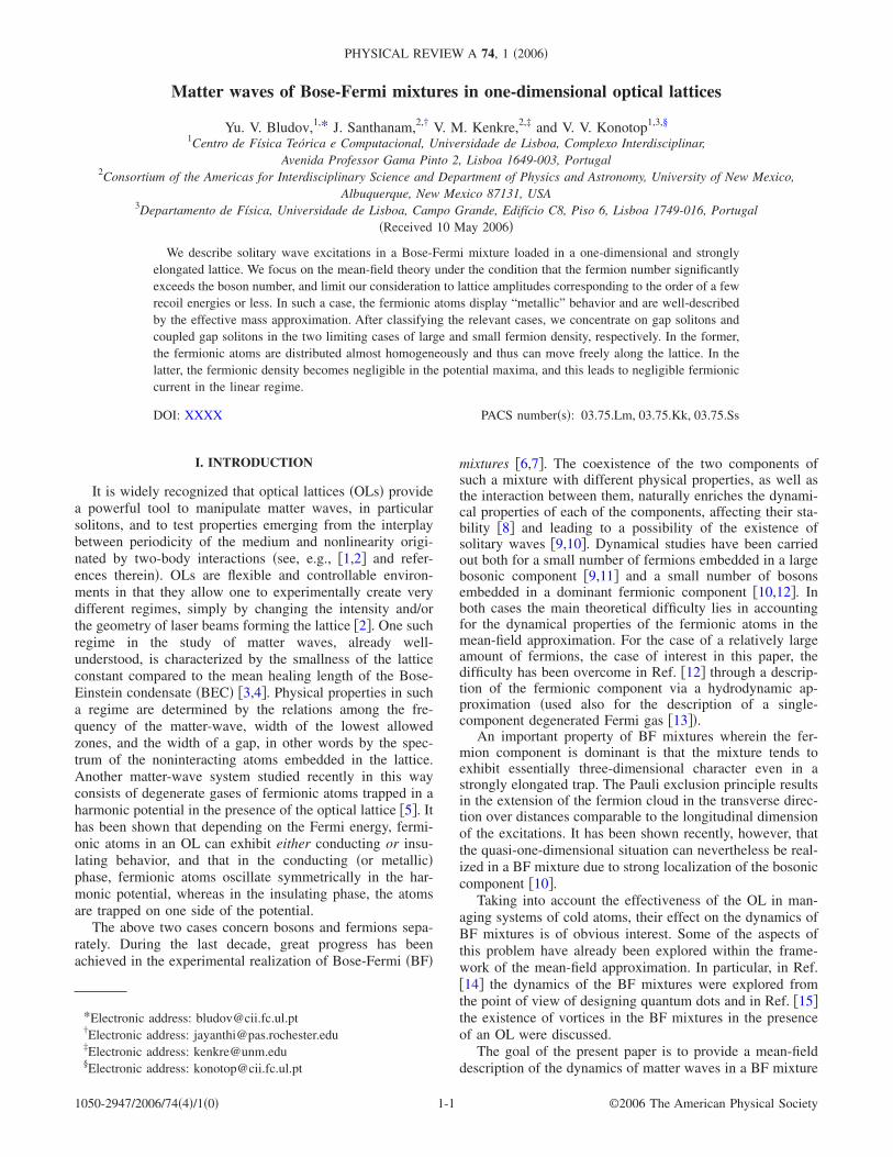
Considering the unperturbed distribution of the fermionsalong the �longitudinal� axis, which is chosen to be x, �i.e., atr�=0�, formula �6� gives an idea about three possible casesfor the distribution of the fermions �they are illustrated inFig. 1�. Namely, we will say that the density of fermions islarge if everywhere along the condensate axis the fermionicdensity significantly differs from zero �the first and secondcolumns in Fig. 1�. Then we still have two possibilities. Thefirst one corresponds to the Fermi energy being much higherthan the lattice amplitude, EF�U f �see the first column, Fig.1�a�� and the difference between the maximal and minimalvalues of the fermion density is small enough �Fig. 1�b�, thefirst column�. In that case in the leading order we can con-sider that the fermion density is independent of the longitu-

TABLE I. Different cases of optical potentials for bosons and fermions addressed in the present paper. Foreach of the cases for bosonic atoms one can associate one of the cases corresponding to the Fermionic atoms.Here we use the dimensionless variables �E, EF, Ub, and U f for the gap in the linear spectrum of bosons, forFermi energy, and for amplitudes of the lattice for bosons and for fermions, respectively. For more detaileddiscussions see the text.

Bosons Fermions

Moderate lattice: Ub1, wide gap: �E�1 Large density, EF�U f �Fig. 1 first column�Moderate lattice: Ub1, narrow gap: �E�1 Large density, EFU f �Fig. 1 second column�Shallow lattice: Ub�1, narrow gap: �E�1 Moderate density, EF�U f �Fig. 1 third column�

FIG. 1. �Color online� Examples of the distributions of the fermionic atoms considered in the present paper and summarized in Table I.The columns from left to right correspond to Uf =−0.2Erf, a=0.5d �the first column�; Uf =−1.5Erf, a=2.0d �the second column�; and Uf

=−3.0Erf, a=3.5d �the third column�. For the sake of convenience the energies are expressed in the units of the fermion recoil energyErf =

�2�2

2mf=MEr�M =mb /mf�. Panels �a� show the band structures �extended zones�, positions of the Fermi energies �solid red horizontal

lines�, and energies of the potential barriers for the fermions �dashed green horizontal lines�. Panels �b� show the cross sections of spatialdistributions of the fermion density at r�=0, computed numerically �solid red curves� and given by the Thomas-Fermi approximation�dashed blue curves� over one period �notice that in panels �b� of the first two columns the difference between the numerical results and theThomas-Fermi approximation are indistinguishable�. The three-dimensional plots show the spatial distributions of the fermions over threeperiods. For all three cases considered above, the number of fermions per lattice period is Nf =104. Details of the numerical calculations areexplained in Appendix A.

MATTER WAVES OF BOSE-FERMI MIXTURES IN ONE-… PHYSICAL REVIEW A 74, 1 �2006�

1-3

dinal coordinate x. The second possibility is shown in thesecond column of Fig. 1, where the Fermi level is still higherthan the OL potential, EFU f �Fig. 1�a�, the second column�,but the difference between values of the fermion density atthe OL potential maxima and minima is considerable. Thenone cannot neglect the x-dependence in the fermion density.In a general situation, both possibilities correspond to themetallic phase of the Fermi component. Indeed, in the firstcase, the Fermi level falls into one of the upper bands, wheregaps are negligibly small. In the second case, the high fer-mionic density can be achieved by increasing the transversedimension of the condensate, making the difference betweenneighboring transverse levels �� f to be less than the upperedge of the largest allowed band �typically of the first lowestband�. Then the lowest energy configuration corresponds topartially filled allowed bands in the longitudinal directionand partially filled transverse levels.

Finally, one can have EF�U f at some points of the x-axis.This case will be referred to as that of moderate density �seethe third column of Fig. 1�. In this case, unperturbed fermi-ons constitute an array of independent condensates located inthe potential minima.

It is worth pointing out that it can be seen from the insets�b� in Fig. 1 that in the cases of large fermion densities thespatial distributions are very well-described by the TF ap-proximation. Visible differences between the results of theTF approximation and the numerically �exact� computed dis-tributions appear in the case of moderate densities, especiallyin the vicinities of the OL potential maxima and minima�Fig. 1�b�, the third column�. However, the difference be-tween the real TF distribution and the approximate formula�6� is still of order of a few percents of the average distribu-tion. It also does not affect the lattice constant. Therefore inthe approximation we will use to treat small-amplitude mat-ter waves �in Sec. VI� the formula �6� will be employed.

D. Dynamical equations

In all the cases considered in the present paper we willneglect the boundary effects of the trap potential in the lon-gitudinal direction. This condition requires the aspect ratios�b,f to be negligibly small, since otherwise the dynamics andeven the form of solitary wave excitations can be signifi-cantly changed �see, e.g., discussion in �1,10��. We thus im-pose �b,f =0.

Since the energy will be measured in units of the recoilenergy, it is natural to introduce the dimensionless variablesR=�r and T= 1

2a2�2�bt where a=�� /mb�b is the trans-verse linear oscillator length of the bosons, and definethe dimensionless macroscopic wave function ��R ,T�= �2�� abb /��r , t�, where ��r , t�= ��, and the di-mensionless density of the fermions: �R ,T�= �6�2M3/2 /�3�nf�r , t�, M =mb /mf, nf�r , t�= �†�� the an-gular brackets stand for the expectation values�.

Then the equation governing the evolution of the bosonsin terms of the macroscopic wave function is obtained by thestandard averaging of Eq. �1�, which in dimensionless vari-ables gives �for the details see, e.g., �12��

i��

�T+ �R� − �b

2R�2 � − Ub�X�� − 2�1�2�

− �2�1 + M�K f �R,T�� = 0. �7�

Here after we use the notations �1,2=sign�g1,2�, �b

=1/ �a��2, K f =2abf�3�M3/2 , and �R ,T�= 0�R�+� �R ,T�, where

0�R� and � �R ,T� are the stationary �background� densityand local perturbation of density of the fermions, respec-tively.

A degenerate fermionic gas can be described in terms ofthe Landau theory of quasiparticles excited in the vicinity ofthe Fermi surface and is governed by the hydrodynamic ap-proximation. The respective equation for the local density ofquasiparticles can be derived directly from Eq. �2� �this isdone in Ref. �12�� and in dimensional variables reads

�2�

�T2 = �R · � 0�R� 4M

3 01/3� + ��2�2�� . �8�

Here we have introduced the dimensionless density in the TFapproximation

0 = �EF − � f2R�

2 − U f�X��3/2, �9�

and defined the parameters � f =� f�b / ��bM1/2� and �=2 abf /abb �1+M�M.

To complete the statement of the problem we now intro-duce the normalization conditions. We will be interested inbright and dark soliton solutions and therefore we distinguishthe normalization conditions for the bosons of the two types.In the case of spatially localized distribution of the bosons�the case of bright solitons� we impose the standard normal-ization condition

�2dR = Nb, Nb = 4�abb�Nb, �10�

where Nb is the total number of bosons and the integral isover the whole space. Formally, a dark soliton solution isconstructed against an infinite background, and therefore thenormalization condition must be written down for the back-ground solution in the absence of the soliton. The conditionis

dR� −�/2

�/2

dX�2 = Nb0, Nb0 = 4�abb�Nb0, �11�

where Nb0=4� abb �Nb0 and Nb0 is an average number ofbosons per OL period.

We will similarly impose the normalization for the back-ground of the fermionic component as

dR� −�/2

�/2

dX 0 = 6�2M3/2Nf , �12�

where Nf is an average number of fermions in a unit cell.


1-4

III. FERMIONS AT LARGE DENSITIES WITH BOSONSIN A LATTICE WITH A LARGE GAP

A. Scaling

Let us start with a moderate size lattice having a wide gapfor bosons and with large density of fermions. This is repre-sented by the first line in Table I and illustrated in the leftcolumn in Fig. 1. We introduce characteristic scales of thetransverse distribution of the bosons and the fermions: Forthe former, Rb=1/��b, which, in dimensionless units, corre-sponds to the transverse oscillator length of the low densityboson component; and for the latter, Rf =�EF /� f, which fol-lows from Eq. �9�. Here, we restrict our considerations to thepotential barrier being of the order of a few recoil energies,i.e., U f �1. This means that EF�1 �see Table I�. Consideringthe linear oscillator frequencies of the bosons and the fermi-ons to be of the same order of magnitude, � f ��b, we obtainthe relation Rf �Rb. On defining the small parameter �= a� �1, where �= �8�nb abb �−1/2 �nb is the maximal density

of bosons�, and requiring �10� Rf2 /Rb

2�EF /� f =�F / �� f�2�,

where �F1 is a parameter of the problem, we can rewriteEq. �9� with accuracy O��3� as

0 � EF3/2�1 −

3�2

2�F�� f

2R�2 + U f cos�2X�� . �13�

At this point we observe that � used in the definition of thesmall parameter is nothing but the healing length when onedeals with dark soliton excitations or sound waves. If, how-ever, bright matter solitons are under considerations, whenthe conventional definition of the healing length is not ap-propriate, � is of order of the mean soliton width. The scalingintroduced above allows us to concentrate on the spatial do-

main, limited in the transverse direction by some radius R,

which satisfies the condition Rb� R�Rf �i.e., by the domainin the transverse direction, where the bosonic component de-cays while the fermionic component changes insignificantly�.Specifically, we impose R=�−1/2.

B. Multiple-scale expansion and 1D equations

Following standard multiple-scale analysis �see, e.g.,�1,10��, we introduce scaled quantities tj =�

jT and xj =�jX,

regarded as independent variables, and look for a solution inthe form of the series

��R,T� = ��1 + �2�2 + �3�3 + O��4� . �14�

Moreover, it is clear from Eq. �8� that � ��2. Using theexpansion for � in the form of Eq. �14�, we find that thevalue � is of the order �2. In other words, � =�2 1, where 1��12.

Substituting the above expansions into Eq. �7� and gath-ering the terms of the same order in �, we rewrite Eq. �7� inthe form of a set of equations �1,3,10�:

�i�

�t0− L�� j = Fj , �15�

where Fj’s are given in Appendix B and depend only on �iwith i� j, and the operator L is given by

L � L� + Lx + �2�1 + M�K fEF3/2, �16�

where

L� = − �� + ��2 R�

2 ,

��2 = �b

2 − �23

2�1 + M�K f�EF� f

2, �17�

Lx = −�2

�x02 + U�x0� ,

U�x0� = Ub�x0� − �23

2�1 + M�K f�EFU f�x0� . �18�

For the next consideration it is important that the scalingchosen guarantees that ��0.

We look for a solution to Eq. �7� which describes a Blochfunction weakly modulated by the nonlinearity present in thetwo-body interactions. Such a solution can be sought in theform

�1 = A�x1,t1��n�x0��R��e−i�0t0, �19�

restricting our considerations to states bordering on the edgeof the first gap �i.e., here either n=0 or n=1�. Note that�n�x0� and ��R�� are defined in Appendix B. The envelopefunction A�x1 , t1� depends on the slow variables,�x1 ,x2 , . . . , t1 , t2 , . . . �, from which only the most rapid areindicated explicitly. The envelope function is independent ofx0, t0, and R�.

Direct substitution leads to the verification that the ansatz�19� satisfies the first �j=1� of Eq. �15� provided

�0 = �2�1 + M�K fEF3/2 + �n + 2��. �20�

Taking into account the wave nature of the discussed phe-nomena throughout this paper �0 will be referred to as afrequency �notice, however, that in the dimensionless units italso can be interpreted as energy or chemical potential,whenever one speaks about stationary solutions�.

Proceeding to the second order of expansion, i.e., to thecomputation of �2, one verifies that it cannot be made zerofor any time. We thus impose a constraint for the density ofbosons to be slowly dependent on time �i.e., to be indepen-dent on t0�. To this end �2 must be searched in the form

�2 = �n��n

Bn��x1,t1��n��x0��R��exp�− i�0t0� . �21�

Substituting this expansion into the second order equationfrom Eq. �15�, and eliminating secular terms by requiring F2to be orthogonal to �n�x�, we find that the envelope functionA is independent of t1, i.e., A=A�x1 , t2�. Furthermore,

�2 =�A

�x1�

n��n

�n�n

�n − �n��n��x0��R��e−i�0t0, �22�

where

�n�n = − 2 −�/2

�/2

�n��x�d

dx�n�x�dx . �23�


1-5

On the other hand, because the equation of the third orderinvolves a dependence on the fermion density, it must besolved together with Eq. �8�. Since the value �12 dependsupon t2, i.e., changes slowly in time, we can find the particu-lar solution of Eq. �8� in the static limit approximation�where �2 1 /�T2=0� in the form

1 = − �2�A�x1,t2�2�n2�2, �24�

where �=3��EF / �4M�. Here we have used the fact that from

Eq. �13�, 1 0

� 0

�X �1 and therefore in the leading order in Eq.�8� we can neglect the dependence of 0 upon the spatialcoordinates.

Comparing the result �24� with the explicit form of �1from Eq. �19�, we find that the same envelope function 1governs both the local fermion density and the boson density.Substituting Eq. �24� in F3 �see Appendix B� and requiringthe absence of secular terms in the third order equation of themultiple scale expansion �i.e., requiring the orthogonality ofF3 and �1�, we find that A�x1 , t2�, satisfies the NLS equation

i�A

�t2+

1

2M�2A

�x12 + �nA2A = 0. �25�

In this NLS equation,

1

2M= 1 + �

n��n

�n�n2

�n − �n��

1

2� �2�n,q

�q2 �q=1

, �26�

�n =��

��EF

1/2�1 + M�2�abf2

2�M3/2�abb− �1��

−�/2

�/2

�n�x�4dx ,

�27�

the quantity �n,q being defined in Appendix B. The effectivemass M characterizes the response of the bosons to the OLpotential—its expression through the dispersion relation canbe obtained by the so-called kp method �18–21�; see also�3�.

C. Bose-Fermi gap solitons

The NLS equation given in Eq. �25� is the main result ofour analysis. To check its experimental feasibility, let us con-sider an example of a Rb87-K40 mixture with characteristicsgiven in Ref. �6�, in a trap with a radial size a�2 �m andOL with a period � /��1 �m. Taking the number of ru-bidium atoms to be 500, and the scattering lengths abb=2 nm and abf =11 nm �16� providing �n�0, we obtain thatthe width of the bright soliton is ��14 �m �see the com-ment after Eq. �13��. This gives �=0.14. From Fig. 1 �thefirst column� after taking into account that the energies aremeasured in units of the fermion recoil energy Erf, and theratio between the fermion and the boson recoil energies isgiven by Erf /Er=M �2.17 for the Rb87-K40 condensate, wealso compute EF�124.2�1. Thus �F�2.43, which is inagreement with the imposed condition �F1 �see formula�13��.

It follows from Eq. �18� that, in a BF mixture, the pres-ence of the fermions can change the effective periodic poten-

tial for the bosons, and, consequently, the value of the gapwidth �E. This effect is illustrated in Fig. 2�a�. Thus if theinteraction between bosons and fermions is repulsive ��2

=1�, the boson-fermion interaction leads to a decrease in thepotential barrier for the bosons. As a result, the value of thegap width becomes narrower in comparison with the situa-tion in which �=0. In the opposite case, when the boson-fermion interaction is attractive ��2=−1�, there is an increasein the effective potential barrier for the bosons. In turn, thegap becomes wider in comparison with the �=0 case.

The BF mixture also exhibits another interesting propertywhich we illustrate in Fig. 2�b�: one can change the effectivepotential barrier for bosons by changing the transverse oscil-lator length. When the transverse linear oscillator length a isincreased �the linear oscillator frequency �b is decreased�,the value of E� decreases. Since � f is of the same order as�b �� f ��b�, this can lead to the lowering of the Fermi en-ergy EF. Equation �18� shows that this, in turn, can result inincreasing or decreasing the effective potential barrier andgap width for bosons when �2 equals 1 or −1, respectively. Itshould be mentioned that in the limit a→�, the value of theeffective potential for bosons tends to Ub, i.e., to the value inthe absence of the boson-fermion interaction. The absolutevalue of the effective mass M �see Fig. 2�c�� decreases �inthe case of the attractive boson-fermion interaction �2=−1�or increases �in the case of the repulsive boson-fermion in-teraction �2=1� with an increase in the transverse linear os-cillator length a. This is a remarkable finding of our analysis.This means that one can change the band gap properties ofthe bosons by changing the transverse oscillator frequency.

When the boson-fermion interaction is turned off ��=0�,the boson and the fermion components are independent ofeach other: the fermion density is given by the TF approxi-mation, Eq. �9�, and the boson system is described by the

(a) (b) (c)

FIG. 2. �Color online� �a� The bosonic band structure �reducedzones� for the two lowest energy bands in the case where the trans-verse linear oscillator length a=2.0d. �b� The dependence of theedges of the bosonic band gap �q=1� on the transverse linear oscil-lator length a. �c� The dependence of the effective mass M at theedges of the bosonic band gap �q=1� on the transverse linear oscil-lator length a. These dependencies were computed for the Rb87-K40,mixture where abf =0.02d, Nf =104 per period, U f =−3.0, Ub=−1.5, and for the cases when the boson-fermion interactions areabsent �solid black curves�, are repulsive �dashed-and-dot redcurves�, and are attractive �dashed blue curves�.


1-6

NLS equation. When ��0, the boson-fermion interactionsalways lead to attractive interactions between the bosons.This consequence of our present analysis is in qualitativeagreement with earlier results �8,10,12�. One can easily findthe critical value of the boson-fermion interaction at whichboth interactions are balanced, i.e., when �n=0:

abfcr = ��

�

2abbEF

1/2

M3/2

�1 + M�2�1/2

. �28�

When abf equals the critical value, the system becomes anideal gas, described by the linear Schrödinger equation. Ifabf is larger than the above critical value, �n�0, the inter-action between bosons and fermions dominates, leading to aneffective attractive interaction between the bosons.

As mentioned above, in the case of periodic lattices, thevalue of the effective mass can be either positive or negativedepending on the region of the Brillouin �reduced� zone �seeFig. 2�c��. Therefore formation of a bright soliton is possibleif M ·�n�0. For the example of the Rb87-K40 mixtureshown in Fig. 2, small amplitude bright solitons can be cre-ated in the vicinity of the edges �0=0.18 �M=−0.28� and�1=1.67 �M=0.13�, for �n�0 and �n�0, respectively. Anexplicit form of the respective solution is obtained directlyfrom Eq. �25� and in dimensionless variables can be writtendown as follows:

�2 = Ab sech2� X

�bs��n�X�2e−��R�

2, �29�

= 0 − �2Af sech2� X

�bs��n�X�2e−��R�

2. �30�

Here

Ab =��

��bs2 �nM

and Af = �Ab �31�

are the amplitudes of the modulations of density profiles forthe bosons and the fermions and �bs characterizes the widthof the soliton and parametrizes the family of the solutions. Aconvenient parametrization useful in experimental applica-tions is given by the total number of bosons, which can bedone using the normalization condition �10�. To this end,taking into account that �n�X� is normalized and is a rapidlyvarying function with respect to the soliton envelope�, weobtain, in leading order, the link

�bs =2

�Nb�nM. �32�

In the vicinity of the edges �0=0.18 �M=−0.28� and �1

=1.67 �M=0.13� �see the example shown in Fig. 2� a darksoliton can be excited if �n�0 and �n�0, respectively. Theexplicit form of the two-component dark soliton solutionreads

�2 = Ab tanh2� X

�ds��n�X�2e−��R�

2, �33�

= 0 − �2Af tanh2� X

�ds��n�X�2e−��R�

2, �34�

where

Ab =��

�

1

�ds2 �nM

and Af = �Ab. �35�

The link between the soliton width �ds and the number ofparticles per unit cell follows from Eq. �11�

�ds =1

�Nb0�nM. �36�

Formally, the expressions for the bright and the dark solitonscoincide with known formulas for the gap solitons in asingle-component bosonic condensate �see, e.g., �1–3��.These solutions have essentially different properties sincethey constitute only a part of the two-component soliton,the second component being a fermionic excitation. As wecan see, the bright and the dark soliton solutions are possiblefor both the boson and the fermion components dependingupon the sign of interactions and the effective mass. Whenthe interaction between bosons and fermions is attractive��2=−1�, we show that both the components can show si-multaneous increase �decrease� in their densities. By con-trast, in the case of repulsive interactions ��2=1� betweenthe components, there is an increase of the density of onecomponent while that of the other decreases.

The above-mentioned difference from the single-component bosonic condensate stems from the fact that thefermionic distribution creates an effective medium for thebosonic solitons. This distribution is very sensitive to thetransverse confinement of the condensate �as illustrated inFigs. 2�b� and 2�c��, and thus can be effectively governed byvariation of the transverse linear oscillator frequency. In par-ticular, by increasing the confinement in the transverse direc-tion, one can increase the Fermi energy EF, thus allowing forthe effective nonlinearity for bosons �n to change the sign�see Eq. �27�� and consequently to change the type of thesoliton.

IV. FERMIONS AT LARGE DENSITIES WITH BOSONSIN A LATTICE WITH AN ARROW GAP

A. Dynamical equations

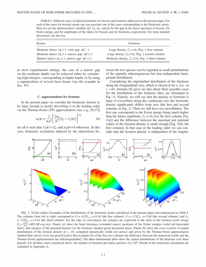
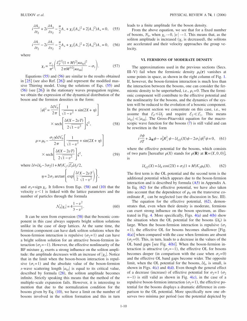
Now we consider the excitations of a BF mixture in adeep lattice for bosons with a narrow band gap. This situa-tion can be realized either when the frequency of the bosonicwave function is large enough or when the OL is created bylaser beams of more than one frequency. To illustrate the firstpossibility, we present an example of the potential in Fig. 3.Alternatively, the fermionic component can originate poten-tials with an arrow gap �see the discussion in Sec. VI�. Theexpansion provided in the previous section cannot be usedfor this case since one has to take into account couplingbetween Bloch states corresponding to the different edges ofthe gap. This coupling is due to the nonlinear interactionsand arises similarly to the situation of gap solitons in photo-


1-7

nic crystals �22� or in nonlinear discrete systems �23�. To bespecific, we assume that a narrow gap is created between thetwo bands n=2 and n=3: �E= �3−�2 � �2,3 where �2 and�3 are the upper boundary of the n=2 band and the lowerboundary of the n=3 band �see Fig. 3�. Using the expansionas shown in �22,23�, we look for a solution to Eq. �7� in theform �cf. Eq. �15��

�1 = �A2�x1,t1��2 + A3�x1,t1��3��e−i�0t0. �37�

Here, as before, An�x1 , t1� �n=2,3� are functions of slowvariables, � and �n are given in Appendix B, and �0 is re-ferred to as a frequency of the soliton. Expression �37� de-scribes the superposition of the modes bordering the narrowbosonic gap. Using the ansatz �37�, in the first order of ��j=1� for the bosons, we find from Eq. �15� at j=1

�0 = �2�1 + M�K fEF3/2 + � + 2��, �38�

where �= ��0+�1� /2 �cf. Eq. �20��.For the next order, we expand �2 over the complete set of

the eigenfunctions of the operator L �cf. Eq. �21��

�2 = �B2�2 + B3�3 + �n�2,3

Bn�n��e−i�0t0, �39�

where Bn=Bn�x1 , t1�. Substituting Eq. �37� and the last rep-resentation in Eq. �15� with j=2, we obtain

�n�

�� − �n��Bn��n� = − i�A2

�t1�2 − 2

�A2

�x1

��2

�x0− i

�A3

�t1�3

− 2�A3

�x1

��3

�x0.

The fact that the right-hand side of this equation must beorthogonal to �2 and �3 yields the two equations

�A2

�t1− iv

�A3

�x1= 0,

�A3

�t1+ iv

�A2

�x1= 0, �40�

where v=�32 is the group velocity of the mode �2+ i�3 inthe limit of the closed gap. For a discussion of this point, see,e.g., �22,23�. The further requirement of the orthogonality

between �1 and �2 yields the relation A2B2+ A3B3=0 �hereand henceforth in this paper an overbar stands for complexconjugation�. It follows from the system �40� that slowlyvarying amplitudes are related to each other as A2= ± iA3,which readily gives the link between B2 and B3: B2=� iB3.Consequently, from Eq. �40�, it follows that A2,3 dependingon x1�vt1.

Let us now fix the direction of propagation of the solutionby choosing the dependence on x=x1−vt1. This correspondsto the branch with A2=−iA3 and B2= iB3, which means thatthe second order term acquires the form:

�2 = ��2 − i�3�B2 + �n�2,3

�n2 − i�n3

� − �n

�n�A2

� x ��e−i�0t0.

Similar to the previous case, we solve Eq. �8� for the fermiondensity 1. After substituting �1 from Eq. �37�, we obtain

1 = − �2��2 + i�32�2A22. �41�

From Eqs. �37� and �41�, we see that both �1 and 1 are nowdetermined by the single envelope function A2.

Using the above result for 1 in the third order equation ofthe multiple scale expansion, i.e., in Eq. �15� with j=3, andrequiring orthogonality of F3 and �1 we find that A2 satisfythe following system of equations:

i�A2

�t2− iv

�A2

�x2+ �D22 − iD23�

�2A2

� x2 + �2A22A2

= − i�B2

�t1− iv

�B2

� x, �42�

i�A2

�t2− iv

�A2

�x2+ �D33 + iD32�

�2A2

� x2 + �3A22A2

= i�B2

�t1+ iv

�B2

� x, �43�

where

Dlm = �lm + �n�2,3

�ln�mn

� − �n

,

and

�l =��

��EF

1/2�1 + M�2�abf2

2�M3/2�abb− �1�

−�/2

�/2

��22 + �3

2��l2dx0.

Here we have taken into account that for symmetric poten-tials �0�X� and �1�X� are real and have different parities.

Taking into account that in a typical case �2��3, andusing the relation between A2 and A3, the variables B2 and B3can be determined from Eqs. �42� and �43�

FIG. 3. �Color online� An example of the band structure with anarrow band gap between bands n=2 and n=3 �solid black lines�.Here �E�0.004 and the potential is Ub=−cos�2X�. The dispersioncurves for the case without OL are depicted by red dash-and-dotcurves. The horizontal dashed curves �green and blue� represent theupper boundary of the n=2 band and the lower boundary of the n=3 band, respectively.


1-8

B3 = − iB2 = −D22 − D33 − 2iD23

4v

�A2

� x. �44�

Using this in Eqs. �42� and �43�, the evolution equation forthe envelope A2 takes the form of the NLS equation

i�A2

�t2+

1

2M�2A2

� x2+ �2A22A2 = 0, �45�

where the effective mass M is determined by

1

M= D22 + D33 =

1

2� �2�2,q

�q2 �q=1

+1

2� �2�3,q

�q2 �q=1

. �46�

Equation �46� shows that the effective mass is determined bythe influence of the remaining Bloch states of the periodiclattice potential on the two given states �in the case underconsideration �2, �3� and also by the mutual influence ofthese two states.

B. Coupled gap solitons and discussion of the results

As in the previous case existence of bright and dark soli-tons is determined by the sign of �2M. If �2M�0, one canobtain a bright soliton solution in the form

��2 =1

4Ab sech2�X − vT

2�bs��2�X�2 + �3�X�2�e−��R�

2,

�47�

= 0 −�2

4Af sech2�X − vT

2�bs��2�X�2 + �3�X�2�e−��R�

2,

�48�

where Ab,f and �bs are given by Eqs. �31� and �32� �with �nsubstituted by �2�. If �2M�0 one obtains a dark solitonsolution

�2 =1

2Ab tanh2�X − vT

�2�ds��2�X�2 + �3�X�2�e−��R�

2,

�49�

= 0 −�2

2Af tanh2�X − vT

�2�ds��2�X�2 + �3�X�2�e−��R�

2,

�50�

where Ab,f and �ds are given by Eqs. �35� and �36�, respec-tively.

We thus see that the result obtained here is qualitativelydifferent from that obtained in the previous section, i.e., fromsingle-mode gap solitons. First of all, a small gap results incoupling of the modes, which makes it impossible to obtain astatic solution �24�. Instead, soliton solutions are constructedagainst a background moving with the velocity v correspond-ing to the group velocity of the carrier wave �2+ i�3. Forinstance, for a potential whose band gap is illustrated in Fig.3, the group velocity v is equal to v�5.988. Second, theabsolute value of the effective mass is bigger than in the caseof single-mode gap solitons, since it is given by the differ-

ence of the effective masses associated with the two gapedges �see Eq. �46�� the effective mass M for the potentialof Fig. 3 is equal to M�0.49�. Finally, we notice that thespatial structure of the carrier wave is weakly pronounced inthe case at hand, since in a typical situation ��2�X�2+ �3�X�2� is weakly dependent on the spatial coordinate.

V. FERMIONS AT LARGE DENSITIESWITH BOSONS IN A SHALLOW LATTICE

Let us now pass to the case of a shallow OL, whereUb�1, an example of which is shown in Fig. 1 �the leftcolumn�. Now the periodic modulation itself must be consid-ered as a perturbation �so, Ub,f =�

2ub,f� and one has to modifythe multiple-scale expansion. This situation is also well-known in the theory of photonic crystals �25�.

In this case, in the multiscale expansion scheme we willseek the solution for ��R ,T� in the form of the series

��R,T� = ��1 + �3�3 + O��4� . �51�

At the same time the series for �R ,T�= �R�+�2 1�R ,T�remains valid. Notice that for a shallow lattice in Eq. �51� theterm proportional to the second power of � is absent �cf. Eq.�14��. The set of equations, obtained from the multiscale ex-pansion �15� will be modified. First, the operator Lx is givenby Lx=− �2

�x02 �cf. Eq. �18��. Second, the equation with j=3

appears as the second order approximation �there is no equa-tion with j=2�. Finally, now F3 is given by

F3 = − i��1

�t2−

�2�1

�x12 − 2

�2�1

�x0 � x2+ u cos�2x0��1

+ 2�1�12�1 + �2�1 + M�K f 1�1, �52�

with u=ub−3�2�1+M�K f�EFuf /2. As we can see from Eq.�52�, the information about the OL potential u appears in amultiscale equation of the third order. As a consequence, themacroscopic wave function for the bosons is given by aweakly modulated superposition of two counterpropagatingplane waves:

�1 =1

��A+eix0 + A−e−ix0��e−i�0t0. �53�

It might be useful here to recall that, in the case of a deep OLwith an arrow gap, the macroscopic wave function for thebosons was represented as a modulation of a superposition oftwo Bloch modes with opposite parity, see Sec. IV. In Eq.�53� as usual, A+�x2 , t2� and A−�x2 , t2� are functions of slowvariables independent of x0, t0, and R�. The factor �−1/2

before exponents is introduced for normalization. Using theansatz �53�, in the first order of � �j=1� for the bosons wefind �0=�2�1+M�K fEF

3/2+1+2��.Taking into account that the expression for the fermion

density 1 after substituting for �1 from Eq. �53� into Eq. �8�will be

1 = − �2�A+eix0 + A−e−ix02�2, �54�

and requiring the orthogonality of F3 to �1, we find that A+and A− satisfy the following system of equations:


1-9

i�A+

�t2+ 2i

�A+

�x2−

u

2A− + �s�A+2 + 2A−2�A+ = 0, �55�

i�A−

�t2− 2i

�A−

�x2−

u

2A+ + �s�A−2 + 2A+2�A− = 0, �56�

where

�s =��

�2�EF1/2�1 + M�2�abf2

2�M3/2�abb− �1� . �57�

Equations �55� and �56� are similar to the results obtainedin �25� �see also Ref. �26�� and represent the modified mas-sive Thirring model. Using the solutions of Eqs. �55� and�56� �see �26�� in the stationary waves propagation regime,we obtain the expression of the dynamical distribution of theboson and the fermion densities in the form:

�2 =UNb

2� � 1�1 − v2

+ sin�2X + �� sech�U�X − 2vT�

2�1 − v2 ��2, �58�

= 0 −�2�UNb

2� � 1�1 − v2

+ sin�2X + �� sech�U�X − 2vT�

2�1 − v2 ��2, �59�

where U=Ub−3�2�1+M�K f�EFU f /2,

� = 2�3 arctan�exp�U2

X − 2vT�1 − v2 �� ,

and �3=sign �s. It follows from Eqs. �58� and �10� that thevelocity v�1 is linked with the lattice parameters and thenumber of particles through the formula

Nb�s = 41 − v2

3 − v2 . �60�

It can be seen from expression �58� that the bosonic com-ponent in this case always supports bright soliton solutionsunlike in the case of deep lattices. At the same time, thefermion component can have dark soliton solutions when theboson-fermion interaction is repulsive ��2=1� and can havea bright soliton solution for an attractive boson-fermion in-teraction ��2=−1�. However, the effective nonlinearity of theBF mixture �s exerts a strong influence on the soliton ampli-tude: the amplitude decreases with an increase of �s. Noticethat in the limit when the boson-boson interaction is repul-sive ��1=1� and the absolute value of the boson-fermions-wave scattering length abf is equal to its critical value,described by formula �28�, the soliton amplitude becomesinfinite. Strictly speaking this means that the method of themultiple-scale expansion fails. However, it is interesting tomention that due to the normalization condition for thebosons given by Eq. �10�, we have a limit on the number ofbosons involved in the soliton formation and this in turn

leads to a finite amplitude for the boson density.From the above equation, we see that for a fixed number

of bosons, Nb, when �s→0, v →1. This means that, as thesoliton amplitude is increased ��s is decreased�, the solitonsare accelerated and their velocity approaches the group ve-locity.

VI. FERMIONS OF MODERATE DENSITY

The approximations used in the previous sections �Secs.III–V� fail when the fermionic density 0�r� vanishes atsome points in space, as shown in the right column of Fig. 1.If, however, the boson-fermion interaction is much less thanthe interaction between the bosons, one can consider the fer-mionic density to be unperturbed, i.e., 1=0. Then the fermi-onic component will contribute to the effective potential andthe nonlinearity for the bosons, and the dynamics of the sys-tem will be reduced to the evolution of a bosonic component.In the present section we concentrate on this case, i.e., weassume that EF�U f and require E2�E1. This meansabf � abb. The Gross-Pitaevskii equation for the macro-scopic wave function for the bosons �7� is still valid and canbe rewritten in the form

i��

�T+ �R� − �b

2R�2 � − Uef f�X�� − 2�1�2� = 0, �61�

where the effective potential for the bosons, which consistsof two parts �hereafter �X� stands for �R� at R= �X ,0 ,0��,is

Uef f�X� = Ub cos�2X� + �2�1 + M�K f 0�X� . �62�

The first term is the OL potential and the second term is theadditional potential which appears due to the boson-fermioninteraction and is described by formula �A5� in Appendix A.In Eq. �62� for the effective potential, we have also takeninto account that the dependence of 0 on the transverse co-ordinate R� can be neglected �see the discussion in Sec. III�.

The equation for the effective potential, �62�, demon-strates that, even when their density is moderate, fermionscan exert strong influence on the boson spectrum, as illus-trated in Fig. 4. More specifically, Figs. 4�a� and 4�b� showthe situation when the OL potential for the bosons �Ub� islarge. When the boson-fermion interaction is repulsive ��2

=1�, the effective OL for bosons becomes shallower �Fig.4�a�� when compared with the case when fermions are absent��2=0�. This, in turn, leads to a decrease in the values of theOL band gaps �see Fig. 4�b��. When the boson-fermion in-teraction is attractive ��2=−1�, the effective OL for bosonsbecomes deeper �in comparison with the case when �2=0�and the effective OL band gaps become wider. The oppositelimit, when the OL potential for the bosons, Ub, is small, isshown in Figs. 4�c� and 4�d�. Even though the general effectof a decrease �increase� of effective potential for �2=1 ��2

=−1� is still valid as shown in Fig. 4�c�, in the case of arepulsive boson-fermion interaction ��2=1�, the effective po-tential for the bosons displays a dramatic difference in com-parison to the OL potential. More specifically now one ob-serves two minima per period �see the potential depicted by


1-10

dash-and-dot lines in Fig. 4�c�. This is due to the fact that thepotential is not “monochromatic” anymore, as it is shown bythe first terms of its Fourier expansion: Uef f�X��0.435+0.008 cos�2X�+0.124 cos�4X�. Here, the second spatialharmonic, cos�4X�, is dominant. This in turn profoundlychanges the band structure of the bosonic spectrum since inthe absence of the second harmonic cos�2X� the Brillouinzone increases becoming �−2,2� and the gap at q= ±1 dis-appears. Now the first harmonic can be considered as a per-turbation of the periodic potential having a period twice aslarge as the period of the original OL. As an example, onecan see from Fig. 4�d�, that, in the case �2=1, the secondband gap �which is located in the vicinity of �=4� is widerthan the first band gap �located in the vicinity of �=1�, con-trary to the case where boson-fermion interactions are ab-sent, i.e., when �2=0.

In the case at hand, bosons just “feel” the change in theeffective periodic potential due to the presence of the fermi-ons. Thus, in the case of moderate fermion density, the bosonsystem can be reduced to either a narrow band gap case�when �2=1� or to a large band gap case �when �2=−1�. Theform of a bosonic soliton is determined either by Eq. �25� �inthe case of a large gap� or by Eq. �45� �in the case of anarrow gap�, with the only difference that now �=0 and�n�x0� are the eigenfunctions of the operator Lx=−�2 /�x0

2

+Uef f�x0�.

VII. CONCLUSION

In the present paper we have considered the formation ofmatter-wave solitons in a Bose-Fermi mixture embedded in aone-dimensional optical lattice and confined by a radiallysymmetric cigar-shaped parabolic trap. We have focused onthe mean-field regime, i.e., supposed that each cell of thelattice contains a large enough number of atoms, and inves-

tigated the case wherein the number of fermions significantlyexceeds the number of bosons. In such a situation, the mix-ture is described by the Gross-Pitaevskii equation for thebosons and by the hydrodynamic equation for the fermions,nonlinearly coupled with each other. The fermions in ourstudy are considered spin-polarized, and thus noninteracting,and therefore the nonlinearity of the system is due to thetwo-body boson-boson and boson-fermion interactions. Wehave shown that, in spite of the essentially three-dimensionalcharacter of the fermion distribution, the evolution equationgoverning the dynamics of the coupled boson-fermion exci-tations can be effectively one-dimensional. The elements re-sponsible for this conclusion are the strong confinement inthe transverse direction and the fact that a small number ofbosons occupies the lowest transverse level. We have alsofound that the boson-fermion interactions result in effectiveattractive interactions among the bosons themselves. Thisfinding agrees with previous studies, can lead to modula-tional instability, and could be used for soliton generation.

We have furthermore shown that the dynamics of small-amplitude solitons is described by the nonlinear Schrödingerequation with an effective mass, in analogy to the standardsituation of pure bosonic condensates loaded in an opticallattice. An essential difference in the present mixture case, inaddition to the significant change of the nonlinearity, is thatthe effective lattice potential is originated by the optical lat-tice and by unperturbed spatial distribution of the fermions.This difference stems from the existence of the fermioniccomponent in the mixture and has two immediate importantconsequences. First, the resulting periodic potential may benonmonochromatic with properties different from those ofthe optical lattice. Second, since the longitudinal distributionof the fermions is highly sensitive to any change in the trans-verse configuration of the trap, a new possibility to manipu-late the solitons appears. This possibility hinges on the�sometimes relatively weak� change of the transverse para-

(a) (b)

(d)

(c)

FIG. 4. �Color online� The effective potentials for the bosons �panels a,c� and the bosonic band structure �reduced zones� for the twolowest energy bands �panels b,d� when the boson-fermion interactions are absent �solid black curves�, are repulsive �dash-and-dot redcurves�, and attractive �dashed blue curves� for the case where af = �M�1/4a=3.5d, abf =0.012d, Nf =104 per period, U f =−6.0 and Ub=−1.5, M =4.0 �panels a,b� or Ub=−0.5, M =12.0 �panels c,d�. The choice of these parameters is determined by the fact that we requireabf � abb to consider the fermion density to be unperturbed and at the same time to obtain considerable influence of the boson-fermioninteraction on the effective potential. Thus we have to compensate the smallness of abf by a high enough value of the relation M=mb /mf. At the same time, we also have U f /Ub�M �such as in �27��.


1-11

bolic trap. Moreover, since the modulational instability isusually considered as a method of generation of solitons, onecan envisage the generation of solitons by means of thechange of the transverse parabolic trap. This was addressedin Ref. �9� in the case of Bose-Fermi mixtures when a rela-tively small number of fermions are embedded in a bosoniccomponent consisting of a much larger number of atoms.However, in this paper, we consider the situation where thenumber of fermions is larger than the number of bosons.Thus the effect of changing the transverse geometry is en-hanced because the fermions generate an effective lattice forthe bosons and thus even a very small change of the trans-verse distribution may have a more dramatic effect on theexistence of the soliton.

We have obtained explicit expressions for gap solitonsand coupled gap solitons in the case of large fermion densi-ties and moderate boson lattices. We have also shown thatbright and dark soliton solutions are possible for both theboson and the fermion components depending upon the signof interactions and the effective mass. �For the fermioniccomponent under the bright soliton we understand the localincrease of the density against an unperturbed distribution,often well-described by the Thomas-Fermi approximation.�In the case of shallow lattices for bosons we have shown thatthe bosonic component always supports bright soliton solu-tions and the fermion component can have bright and darksoliton solutions depending on the boson-fermion interac-tion. For the sake of convenience, the soliton solutions ob-tained for the different cases considered in this paper aresummarized in Table II.

We thus conclude that one has a large diversity of mattersolitons even when OL is deep enough, i.e., of the order of afew recoil energies: the fermionic component can make theeffective potential shallow or contribute to shrinking some ofthe gaps. Each of these cases requires modification of theasymptotic expansion needed for the description of the soli-tons and thus originates solitons with different properties. Tothe best of our knowledge, the respective solitons in purebosonic condensates �where the potential is created, say, ei-

ther by low-intensity laser beams or by a superposition oflaser beams of different frequencies� have not been consid-ered in the literature, so far. The respective results, however,can be easily obtained from those presented in this paper byimposing the scattering length of boson-fermion interactionsto be zero.

In all the cases considered in the present paper, the fermi-onic component was considered in the metallic phase. Thiswas justified by a large number of fermions and by the trans-verse confinement making the distance between the trans-verse energy levels to be less than widths of the energybands. This naturally means that the present research doesnot exhaust relevant experimentally feasible possibilitieseven in the regime of the mean-field approximation. In par-ticular, we did not consider the cases of deep optical lattices,where the allowed bands are very narrow, the fermionic com-ponent is in the insulator phase, and the bosonic componentis localized on a very few lattice periods giving rise to theintrinsic localized modes �or breathers�.

ACKNOWLEDGMENTS

Y.V.B. was supported by the FCT, SFRH/PD/20292/2004.The work of Y.V.B. and V.V.K. was supported by the FCTand European program FEDER under the grant POCI/FIS/56237/2004. V.M.K. acknowledges partial support ofDARPA under DARPA-N00014-03-1-0900 and the NSF un-der INT-0336343.

APPENDIX A: DIRECT COMPUTATIONOF THE UNPERTURBED DISTRIBUTION

OF FERMIONS

To find the unperturbed density distribution of the spin-polarized fermions, we use the following approximations: �i�the fermions are spin-polarized and thus noninteracting and�ii� the trap is long enough in the direction of the opticallattice, thus allowing us to neglect boundary effects, or inother words to consider the spacial ratio � f =0 in Eq. �4� and

TABLE II. Summary of the linear atomic densities for bosons and fermions obtained for different parameters of the optical lattice forbosons. In the boxes below the analytical expressions of the solitons, we indicate their type, as well as the respective formula in the text.Bright solitons of the fermionic component are understood as a local increase of the fermionic density against a background. For detaileddiscussion and notations see the text.

Lattice Gap Distribution of bosons�2 Distribution of fermions

Ab

cosh2�X/�bs��n�X�2

Bright soliton; Eq. �29� 0−

�2Af

cosh2�X/�bs��n�X�2

Bright �dark� soliton for �2�0 ��2�0�; Eq. �30�ModerateUb�Er

Large�E�E1,2

Ab tanh2� X�ds

� �n�X�2

Dark soliton; Eq. �33� 0−�2Af tanh2� X

�bs� �n�X�2

Bright �dark� soliton for �2�0 ��2�0�; Eq. �34�Ab

4 cosh2�X−vT/2�bs��2�X�2+ �3�X�2�


�2Af

cosh2��X−vT�/2�ds��2�X�2+ �3�X�2�

Bright �dark� soliton for �2�0 ��2�0�; Eq. �48�Narrow�E�E1,2

Ab

2 tanh2� X−vT�2�ds

��2�X�2+ �3�X�2�Dark soliton; Eq. �49�

0−�2

2 Af tanh2� X−vT�2�bs

��2�X�2+ �3�X�2�Bright �dark� soliton for �2�0 ��2�0�; Eq. �50�

ShallowUb�Er

Narrow�E�E1,2

UNb

2�

��1/�1−v2�+sin�2X+��

cosh(U�X−2vT�/2�1−v2)


�2�NbU2�

��1/�1−v2�+sin�2X+��

cosh�U�X−2vT�/2�1−v2�Bright �dark� soliton for �2�0 ��2�0�; Eq. �59�


1-12

substitute zero boundary conditions at infinity by the peri-odic boundary conditions. Then the single-particle wavefunction q,m�r� solves the Schrödinger equation:

−�2

2mf� q,m +

mf

2�2r�

2 q,m = Eq,m q,m, �A1�

and thus can be represented in the form

q,m = e−r�2 /2af

2Hmy

� y

af�Hmz

� z

af�

af�2my+mzmy ! mz ! �

�p=−�

�

cp�q�eiqx+2ip�x,

�A2�

where m= �my ,mz� are the transverse quantum numbers, q= �q ,!� where q and ! are the wave vector in the first BZ andthe number of the zone, respectively, af = �� /mf� f�1/2 is thetransverse linear oscillator length of the fermionic compo-nent; Hm�·� are the Hermit polynomials, and � is related tothe lattice constant d as defined in Sec. II of the text. Thecorresponding energy eigenvalues are given by Eq,m=Ex�q�+ �� f�my +mz+1�. The coefficients cp�q� and Ex�q� can beobtained as the eigenvalues of the matrix

Hp,p� =�2�q + 2p��2

2mf�p,p� +

Uf

2��p,p�+1 + �p,p�−1�

i.e.,

�p�

�Hp,p� − �pp�Ex�cp��q� = 0. �A3�

The Fermi radius can be found, supposing, that in the phasespace the number of fermions per one-dimensional shelldxdq is equal to dn=dxdq / �2��. Assuming that the numberof fermions Nf is large, we represent the equation for theFermi energy in the form

Nf =1

2��s=0

smax

�s + 1� −gs

gs

dq −d/2

d/2

dx =1

��s=0

smax

�s + 1�gs,

where gs are determined from the equation EF= �� f�s+1�+Ex�gs�, smax= �EF / �� f�−1 �here the square brackets standfor the integer value� is the number of the highest filled en-ergy level of transverse quantization, the factor s+1 appearsdue to the transverse quantization level degeneracy.

Similarly, to find the spatial distribution of the fermiondensity we integrate the absolute value of the square of thewave functions �A2� over all occupied states:

n�r�exp�−

r�2

af2 �

�2af2 �

s=0

smax

�t=0

s Ht2� y

af�Hs−t

2 � z

af�

2st ! �s − t�!

� 0

gs � �p=−�

�

cp�q�ei2p�x�2

dq . �A4�

At y=z=0 the formula �A4� can be rewritten as

n�x,0,0� =1

�2af2 �

s=0

�smax/2�

�t=0

s�− 1�s

2s�2t� ! ! �2s − 2t� ! !

� 0

g2s � �p=−�

�

cp�q�ei2p�x�2

dq . �A5�

Notice that if

−d/2

d/2 ��p

cp�q�ei2p�x�2dx = d �A6�

�or, equivalently, �p cp�q�2=1�, the normalization condition

dr� −d/2

d/2

dx n�r� =1

��s=0

smax

�s + 1�gs = Nf

is met.

APPENDIX B: ON THE MULTIPLE SCALE EXPANSION

For the sake of completeness here we present some detailsof the multiple-scale expansion used throughout the text.

The first three functions Fj �j=1,2 , . . . � in the right-handside of Eq. �15� are given by F1=0,

F2 = − i��1

�t1− 2

�2�1

�x0 � x1,

F3 = − i��1

�t2− 2

�2�1

�x0 � x2−

�2�1

�x12 − i

��2

�t1− 2

�2�2

�x0 � x1

+ 2�1�12�1 + �2�1 + M�K f 1�1

where j=1,2 , . . . coincides with the order of � at which theequation is obtained.

Next we define the eigenfunctions �n,q�x� of the operatorLx: Lx�n,q�x0�=�n,q�n,q�x0�, where n and q refer to the bandnumber and to the wave vector in the first Brillouin zone. Forthe Bloch functions bordering an edge of the Brillouin zone,i.e., for q= ±1, we introduce the notation �n�x��n,±1�x�.These functions are real. Next we consider the eigenvalueproblem for the 2D harmonic oscillator L��lm�R��= �2�l+m+1��lm�R�� and for its ground state we introduce thenotation �R�= R� �

��R�� 0,0�R�� = ��

��1/2

e−1/2��R�2

. �B1�


1-13

�1� V. A. Brazhnyi and V. V. Konotop, Mod. Phys. Lett. B 18, 627�2004�.

�2� O. Morsch and M. Oberthaler, Rev. Mod. Phys. 78, 179�2006�.

�3� V. V. Konotop and M. Salerno, Phys. Rev. A 65, 021602�R��2002�.

�4� H. Pu, L. O. Baksmaty, W. Zhang, N. P. Bigelow, and P. Mey-stre, Phys. Rev. A 67, 043605 �2003�; A. V. Yulin, D. V. Skry-abin, and P. S. J. Russel, Phys. Rev. Lett. 91, 260402 �2003�;H. Sakaguchi and B. A. Malomed, J. Phys. B 37, 1443 �2004�;B. J. Dabrowska, E. A. Ostrovskaya, and Yu. S. Kivshar, J.Opt. B: Quantum Semiclassical Opt. 6, 423 �2004�.

�5� L. Pezzè, L. Pitaevskii, A. Smerzi, S. Stringari, G. Modugno,E. DeMirandes, F. Ferlaino, H. Ott, G. Roati, and M. Inguscio,Phys. Rev. Lett. 93, 120401 �2004�.

�6� G. Mundugno, G. Roati, F. Riboli, F. Ferlaino, R. J. Brecha,and M. Iguscio, Science 297, 2240 �2002�.

�7� F. Schreck, G. Ferrari, K. L. Corwin, J. Cubizolles, L. Khayk-ovich, M.-O. Mewes, and C. Salomon, Phys. Rev. A 64,011402�R� �2001�.

�8� R. Roth, Phys. Rev. A 66, 013614 �2002�.�9� T. Karpiuk, M. Brewczyk, S. Ospelkaus-Schwarzer, K. Bongs,

M. Gajda, and K. Rzazewski, Phys. Rev. Lett. 93, 100401�2004�.

�10� J. Santhanam, V. M. Kenkre, and V. V. Konotop, Phys. Rev. A73, 013612 �2006�.

�11� T. Karpiuk, M. Brewczyk, and K. Rzazewski, Phys. Rev. A 69,043603 �2004�.

�12� T. Tsurumi and M. Wadati, J. Phys. Soc. Jpn. 69, 97 �2000�.�13� G. M. Bruun and C. W. Clark, Phys. Rev. Lett. 83, 5415

�1999�.�14� M. Salerno, Phys. Rev. A 72, 063602 �2005�.�15� M. Centelles, M. Guilleumas, M. Barranco, R. Mayol, and M.

Pi, Laser Phys. 16, 360 �2006�.�16� F. Ferlaino, C. D’Errico, G. Roati, M. Zaccanti, M. Inguscio,

G. Modugno, and A. Simoni, Phys. Rev. A 73, 040702�R��2006�.

�17� K. Mølmer, Phys. Rev. Lett. 80, 1804 �1998�.�18� M. A. Morrison, T. L. Estle, and N. F. Lane, Quantum States of

Atoms, Molecules, and Solids �Prentice-Hall, EnglewoodCliffs, NJ, 1976�.

�19� J. Kevorkian and J. D. Cole, Multiple Scale and Singular Per-turbation Methods �Springer, New York, 1996�, Chap. 6.

�20� H. Pu, L. O. Baksmaty, W. Zhang, N. P. Bigelow, and P. Mey-stre, Phys. Rev. A 67, 043605 �2003�.

�21� N. W. Ashcroft and N. D. Mermin, Solid State Physics �Saun-ders College Publishing, Fort Worth, TX, 1976�.

�22� V. V. Konotop and G. P. Tsironis, Phys. Rev. E 53, 5393�1996�.

�23� V. V. Konotop, Phys. Rev. E 53, 2843 �1996�; S. Jiménez andV. V. Konotop, Phys. Rev. B 60, 6465 �1999�.

�24� This phenomenon was observed in numerical studies of wavepropagation in photonic crystals by J. Peyraud and J. Coste,Phys. Rev. B 40, 12201 �1989�.

�25� A. B. Aceves and S. Wabnitz, Phys. Lett. A 141, 37 �1989�.�26� A. I. Maimistov and A. M. Basharov, Nonlinear Optical Waves

�Kluwer Academic Publishers, Dordrecht, The Netherlands,1999�.

�27� G. Modugno, F. Ferlaino, R. Heidemann, G. Roati, and M.Inguscio, Phys. Rev. A 68, 011601�R� �2003�.


1-14

Matter waves of Bose-Fermi mixtures in one-dimensional...

Documents

Transcript of Matter waves of Bose-Fermi mixtures in one-dimensional...