MATROID FILTRATIONS AND COMPUTATIONAL PERSISTENT HOMOLOGYghrist/preprints/Eirene.pdf · MATROID...

MATROID FILTRATIONS AND COMPUTATIONAL PERSISTENTHOMOLOGY

GREGORY HENSELMAN AND ROBERT GHRIST

ABSTRACT. This technical report introduces a novel approach to efficient com-putation in homological algebra over fields, with particular emphasis on com-puting the persistent homology of a filtered topological cell complex. The algo-rithms here presented rely on a novel relationship between discrete Morse theory,matroid theory, and classical matrix factorizations. We provide background, de-tail the algorithms, and benchmark the software implementation in the EIRENE

package.

1. INTRODUCTION

This paper reports recent work toward the goal of establishing a set of efficientcomputational tools in homological algebra over a field [13]. Our principal moti-vation is to improve upon the foundation built in [6] and develop and implementefficient algorithms for computing cosheaf homology and sheaf cohomology in thecellular setting. One can specialize to constructible cosheaf homology over thereal line, which includes persistent homology as a particular instance. As this in-cidental application is of particular current relevance to topological data analysis[5, 8, 10, 11, 19, 22], we frame our methods to this setting in this technical report.

We present a novel algorithm for computing persistent homology of a filteredcomplex quickly and memory-efficiently. There are three ingredients in our ap-proach.

(1) Matroid theory. Our algorithms are couched in the language of matroids,both for elegance and efficiency. This theory permits simple reformulationof standard notions of persistence [filtrations, barcodes] in a manner thatincorporates matroid concepts [rank, modularity, minimal bases] and theconcomitant matroid algorithms.

(2) Discrete Morse theory. It is well-known [2, 3, 7, 15, 16] that discreteMorse theory can be used to perform a simplification of the complex whilepreserving homology. We build on this to use the Morse theory to avoidconstruction and storage of the full boundary operator, thus improvingmemory performance.

Date: June 1, 2016.1

http://gregoryhenselman.org/eirene.html

2 GREGORY HENSELMAN AND ROBERT GHRIST

(3) Matrix factorization. Combining matroid and Morse perspectives withclassical matrix factorization theorems allows for both more efficient com-putation as well as the ability to back-out representative generators of ho-mology as chains in the original input complex, a capability of significantinterest in topological data analysis.

This technical report is intended for a reader familiar with homology, persistenthomology, computational homology, and (elementary) discrete Morse theory: assuch, we pass over the usual literature review and basic background. Since (inthe computational topology community) matroid theory is much less familiar, weprovide enough background in §2 to explain the language used in our algorithms.Matrix reformulation of persistence and subsequent algorithms are presented in§3-§6. Implementation and benchmarking appears in §7.

2. BACKGROUND

For the purpose of continuity it will be convenient to fix a ground field k, tobe referenced throughout. Given a k-vector space V and a set inclusion S ↪→ V ,we write 〈S〉 for the subspace spanned by S and V/S for the quotient of V by 〈S〉.Where context leaves no room for confusion we will identify the elements of Vwith their images under quotient maps, making it possible, for example, to speakunambiguously of the linear independence of T in V/S. Given an arbitrary set Eand singleton { j}, we write E + j for E ∪{ j}, and given any binary relation R onE we write Rop for {(t,s) : (s, t) ∈ R}.

We review the elements of finite matroid theory, full details of which may befound in a number of excellent introductory texts [4, 20, 21, 25]. The readershould note that while, for historical reasons, most authors restrict scope of theterm matroid to that of finite matroids, a number of generalizations to the infinitesetting have been proposed. Among these the finitary matroids of finite rank suitour purposes best, and we refer to finite-rank, finitary matroids implicitly wherevermatroids appear in the text.

With that preface, a (finite-rank, finitary) matroid M consists of a pair (E,I),where E is a set, I ⊆ 2E is a family of subsets, and (i) J ∈ I whenever I ∈ I andJ ⊆ I, and (ii) if I,J ∈ I with |I|< |J|, then there exists j ∈ J− I such that I+ j ∈ I.The sets E and I, sometimes written E(M) and I(M) to emphasize associationwith M, are called the ground set and independence system, respectively. The ele-ments of I are independent sets and those of 2E−I are dependent. Maximal-under-inclusion independent sets are bases and minimal-under-inclusion dependent setsare circuits. It follows directly from the axioms that a singleton {e} forms a circuitif and only if the replacement set

R(e→ B) = {b ∈ B : B−b+ e ∈B(M)}is empty for some basis B. The family of all bases is denoted B(M), and that of allcircuits is denoted C(M).

The conditions imposed by (ii) on I(M),B(M), and C(M) support a remarkablebranch of combinatorics, with fundamental ties to discrete and algebraic geome-try, optimization, algebraic and combinatorial topology, graph theory, and analysis

MATROID FILTRATIONS AND COMPUTATIONAL PERSISTENT HOMOLOGY 3

of algorithms. They also underlie a number of the useful properties associatedwith finite-dimensional vector spaces, many of which, including dimension, havematroid-theoretic analogs.

To illustrate, consider a matroid found very often in literature: that of a subsetU in a finite-dimensional, k-linear vector space V . To every such U correspondsan independence system I consisting of the k-linearly independent subsets of U ,and it is an elementary exercise to show that the pair M(U) = (U,I) satisfies theaxioms of a finite-rank, finitary matroid. We will introduce the next group of termswith explicit reference to this construction.

Zero We say e ∈ E is a zero element if {e} ∈ C(M). As remarked above, the zeroelements are those for which the set R(e→ B) is empty. Clearly u ∈U is a zero inM(U) if and only if u = 0 ∈V .

Rank Axiom (ii) can be shown to imply that |I| = |J| for every pair of maximal-with-respect-to-inclusion independent subsets of an arbitrary S⊆ E. This number,denoted ρ(S), is called the rank of S. By convention ρ(M) = ρ(E). If M = M(U),then ρ(S) = dim〈S〉.

Closure The closure of S ⊆ E, written cl(S), is the discrete analog of a subspacegenerated by S in V : formally, S is set of all e ∈ E such that {e}=C−S for someC ∈ C(M). If M = M(U), then S = U ∩ 〈S〉. A flat is a subset that contains itsclosure.

Deletion If S⊆ E then the family I= {T ∈ I(M) : T ⊆ E−S} is the independencesystem of a matroid M−S on ground set E−S, called the deletion of M by S. Therestriction of M to S, written M|S, is the deletion of M by E−S. If M = M(U) thenM|S = M(S).

Contraction The contraction of M by S, denoted M/S, is the matroid on ground setE−S with independence system {T ∈ I(M) : T ∪J ∈ I ∀ J ∈ I∩2S}. For the pur-pose of our discussion it is worth noting an alternate characterization of I(M/S): ifI is a maximal independent subset of S, then I(M/S) = {J ⊆ E−S : J∪ I ∈ I(M)}.As an immediate corollary, ρ(M/S) = ρ(M)− ρ(S). If M = M(U) then M/S isthe matroid generated by U−S in the quotient space V/〈S〉.

Minor Matroids obtained by sequential deletion and contraction operations are mi-nors of M. It can be shown that deletion and contraction commute, so that everyminor may be expressed (M− S)/T for some S and T . Where context leaves noroom for confusion we write S/T for (M|S)/T .

Representation A (k-linear) representation of M is a map φ : E→kr such that I ∈ Iif and only if φ(I) is linearly independent. Matroids that admit k-linear representa-tions are called k-linear. It is common practice to identify a representation E→ kr

with the matrix A ∈ k{1,...,r}×E such that A[ : ,e] = ϕ(e) for all e ∈ E. In general,


we will not distinguish between A and the associated E-indexed family of columnvectors. Given B ∈ B(M), we say ϕ has B-standard form if ϕ(B) is the basis ofstandard unit vectors in kr. Clearly B-standard representations of M(kr) are in 1-1correspondence with GLr(k).

We note a few facts regarding discrete optimization. Let f : E → R be anyweight function, S ⊆ eE be any family of subsets, and B ⊆ S be the family ofmaximal-under-inclusion elements of S. The elements of argmaxB∈B f (B), wheref (B) = ∑b∈B f (b), are of fundamental importance to a number of fields in discretegeometry and combinatorics, and the problem of finding the maximal B given E, f ,and an oracle to determine membership in S has been vigorously studied sincethe mid-20th century. This problem, NP-hard in general, admits a highly efficientgreedy solution in the special case where (E,S) constitutes a matroid. In fact, thischaracterizes finite matroids completely. The following is classical:

Proposition 1. Let E be a finite set and S be a subset of 2E closed under inclusion.Then S is the independence system of a matroid on ground set E if and only ifAlgorithm 1 returns an element of argmaxS f for arbitrary f : E→ R.

Proposition 1 affords a number of efficient proof techniques in the theory offinite matroids (as will be seen). As argminS f = argmaxS(− f ), Algorithm 1 alsoprovides a greedy method for obtaining minimal bases, which will be of primaryconcern.

Algorithm 1 Greedy algorithm for maximal set-weight

1: Label the elements of E by e1, . . . ,en, such that f (ei+1)≤ f (ei).2: S := /03: for i = 1, . . . ,n do4: if S+ s ∈ S then5: S← S+ s6: end if7: end for

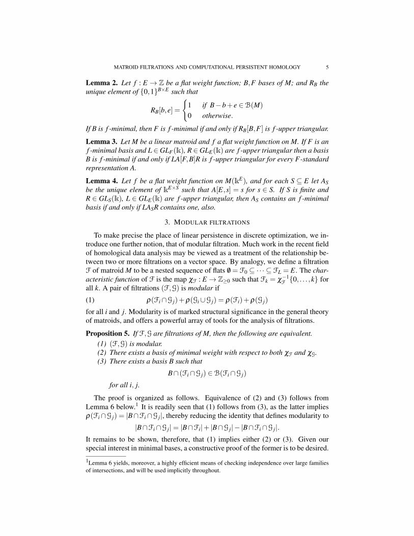
Our final comments concern the relationship between a pair of f -minimal bases.Up to this point, the terms and observations introduced have been standard ele-ments of matroid canon. In the following sections we will need two new notions,namely those of a flat function and an f -triangular matrix.

Given S,T ⊆ E and f : E→Z, say that A∈ kS×T is f -upper triangular if f [s]≤f [t] whenever A[s, t] is nonzero. The product of two f -upper triangular matricesis again upper-triangular, as are their inverses. We say A is f -lower triangular ifit is g-upper triangular for g = − f , and f -diagonal if it is f -upper and f -lowertriangular. We say f is flat if the inverse image f−1(−∞, t] is a flat of M for everychoice of t.


Lemma 2. Let f : E → Z be a flat weight function; B,F bases of M; and RB theunique element of {0,1}B×E such that

RB[b,e] =

{1 if B−b+ e ∈B(M)

0 otherwise.

If B is f -minimal, then F is f -minimal if and only if RB[B,F ] is f -upper triangular.

Lemma 3. Let M be a linear matroid and f a flat weight function on M. If F is anf -minimal basis and L∈GLF(k), R∈GLE(k) are f -upper triangular then a basisB is f -minimal if and only if LA[F,B]R is f -upper triangular for every F-standardrepresentation A.

Lemma 4. Let f be a flat weight function on M(kE), and for each S ⊆ E let ASbe the unique element of kE×S such that A[E,s] = s for s ∈ S. If S is finite andR ∈ GLS(k), L ∈ GLE(k) are f -upper triangular, then AS contains an f -minimalbasis if and only if LASR contains one, also.

3. MODULAR FILTRATIONS

To make precise the place of linear persistence in discrete optimization, we in-troduce one further notion, that of modular filtration. Much work in the recent fieldof homological data analysis may be viewed as a treatment of the relationship be-tween two or more filtrations on a vector space. By analogy, we define a filtrationF of matroid M to be a nested sequence of flats /0 = F0 ⊆ ·· · ⊆ FL = E. The char-acteristic function of F is the map χF : E→ Z≥0 such that Fk = χ

−1F {0, . . . ,k} for

all k. A pair of filtrations (F,G) is modular if

ρ(Fi∩G j)+ρ(Gi∪G j) = ρ(Fi)+ρ(G j)(1)

for all i and j. Modularity is of marked structural significance in the general theoryof matroids, and offers a powerful array of tools for the analysis of filtrations.

Proposition 5. If F,G are filtrations of M, then the following are equivalent.(1) (F,G) is modular.(2) There exists a basis of minimal weight with respect to both χF and χG.(3) There exists a basis B such that

B∩ (Fi∩G j) ∈B(Fi∩G j)

for all i, j.

The proof is organized as follows. Equivalence of (2) and (3) follows fromLemma 6 below.1 It is readily seen that (1) follows from (3), as the latter impliesρ(Fi∩G j) = |B∩Fi∩G j|, thereby reducing the identity that defines modularity to

|B∩Fi∩G j|= |B∩Fi|+ |B∩G j|− |B∩Fi∩G j|.It remains to be shown, therefore, that (1) implies either (2) or (3). Given ourspecial interest in minimal bases, a constructive proof of the former is to be desired.

1Lemma 6 yields, moreover, a highly efficient means of checking independence over large familiesof intersections, and will be used implicitly throughout.


Lemma 6. A basis B has minimal weight with respect to χF and χG if and only if

B∩ (Fi∩G j) ∈B(Fi∩G j)(2)

for all i, j.

Proof. If B satisfies (2) for all i, j then minimality with respect to F follows from anapplication of Lemma 6 to the family of intersections B∩Fi∩E. Minimality withrespect to B follows likewise. If on the other hand S = B∩ (Fi∩G j) /∈B(Fi∩G j)for some i, j, then there exists s ∈ Fi∩G j such that S+ s ∈ I(M). The fundamentalcircuit of s with respect to B intersects B−S nontrivially, hence B−b+ s ∈B(M)for some b ∈ B−S. Either χF(s) < χF(b) or χG(s) < χG(b), and the desired con-clusion follows. �

Proof of Proposition 5. As already discussed, it suffices to show (1) implies (2).Therefore assume (F,G) is modular, and for each i fix a χG-minimal

Bi ∈B(Fi/Fi−1).

The union B = ∪iBi ∈B(M) forms a χF-minimal basis in M, so it suffices to showB is minimal with respect to G. Since |B∩G j| ≤ ρ(G j), we may do so by proving|B∩G j| ≥ ρ(G j) for all j. Therefore let i and j be given, fix Si−1 ∈ B(Fi−1∩G j)and extend Si−1 to a basis Si of Fi∩G j.

Modularity of (Fi,G j) implies

ρ(G j/Fi) = ρ(G j ∪Fi)−ρ(Fi) = ρ(G j)−ρ(G j ∩Fi) = ρ(G j/(G j ∩Fi)),

so that, for all i and j,

ρ(G j/Fi) = ρ(G j/(Fi∩G j)) = ρ(G j/Si)≤ ρ(G j/(Si∪Fi−1))≤ ρ(G j/Fi).

As the quantities on either side are identical, strict equality holds throughout. Thusthe second equality below.

ρ(G j/Si−1)−ρ(Si/Si−1) = ρ(G j/Si)

= ρ(G j/(Si∪Fi−1) = ρ(G j/Fi−1)−ρ(Si/Fi−1).

A comparison of left- and right-hand sides shows ρ(Si/Si−1) = ρ(Si/Fi−1). Byconstruction the set Ti j = Si−Si−1 ∈ G j∩Fi−Fi−1 forms a basis in Si/Si−1, hence

|Ti j|= ρ(Si/Si−1) = ρ(Si/Fi−1) = ρ(Ti j/Fi−1).

Thus Ti j ∈ I(Fi/Fi−1), so |Bi∩G j| ≥ |Ti j|. A second and third application of mod-ularity provide the second and third equalities below,

|Ti j|= ρ(G j/Si−1)−ρ(G j/Si)

= ρ(G j/Fi−1)−ρ(G j/Fi)

= ρ(G j ∩Fi)−ρ(G j ∩Fi−1)

whence |Bi∩G j| ≥ ρ(G j ∩Fi)−ρ(G j ∩Fi−1). Summing over i yields

|B∩G j| ≥ ρ(G j)

which was to be shown. �


4. LINEAR FILTRATIONS

We now specialize to the case of linear filtrations. Recall that a linear fil-tration of a finite-dimensional vector space V is a nested sequence of subspaces/0 = F0 ⊆ ·· · ⊆ FL =V . Clearly, the linear filtrations of V are exactly the matroid-theoretic filtrations of M(V ). Since dimFi + dimG j = dimFi∩G j + dim〈Fi∪G j〉when F and G are linear, Proposition 5 implies that to every such pair correspondsa basis B ∈B(M) such that Fi∩G j = 〈B∩Fi∩G j〉 for all i, j. We are interested incomputing B when V = kr.

Assume that the data available for this pursuit are (1) an F-minimal basis F , (2) afinite set G containing a χG-minimal basis, and (3) oracles to evaluate χF on F andχG on G. These resources are commonly accessible for computations in persistenthomology, as described in the following section. One can assume, further, that Fis the set of standard unit vectors in V = kF . If such is not the case one can solvethe analogous problem for an F-standard representation ϕ ∈ GL(V ), and port thesolution back along ϕ−1. Our strategy will be to construct a (χF,χG)-minimal basisfrom linear combinations of the vectors in G. A few pieces of notation will aid itsdescription.

Given a matrix A ∈ kF×G, write supp s and supp t for the supports of row andcolumn vectors indexed by, s and t, respectively. Say that a relation R on E respectsf : E → R, or that R is an f -relation, if f (s) ≤ f (t) whenever (s, t) ∈ R. Given aχF-linear order <F and a χG-linear order <G, define P, S, and T by

P= {( f ,g) : f = max<Fsuppg, g = min<G

supp f}S = { f : ( f ,g) ∈ P(A,<F,<G) for some g}T = {g : ( f ,g) ∈ P(A,<F,<G) for some f}

and L, R, X , Y , Z, and ∗ by

L =S Sc

S X−1 0Sc −X−1Z I

A =T T c

S X YSc Z ∗

R =T T c

T I −X−1YT c 0 I

where Sc = F − S and T c = G− T . It can be helpful to regard P as the Pareto-optimal frontier of supp A = {(s, t) : A[s, t] 6= 0}with respect to <G and the inverse-order <F

op. See Figure 1.Lemma 7 now holds by construction.

Lemma 7. If P, S, and T are as above, then

(1) L is χF-lower-triangular,(2) R is χG-upper-triangular, and(3) The product LAR satisfies

LAR =T T c

S I 0Sc 0 ∗

for some block-submatrix ∗ of rank equal to rank A−|S|.


Where convenient we will write L(A,<F,<G), R(A,<F,<G), and P(A,<F,<G)for L,R, and P to emphasize association with their genera. In the description ofAlgorithm 2 we will write Lt and Rt for values of L and R associated to At .

Algorithm 2 Matrix reduction1: for t = 1, . . . ,r do2: At+1← LtAtRt3: if |At+1|∞ = r then4: break5: end if6: end for

The proof of Lemma 8 follows easily from Lemma 7:

Lemma 8. Stopping condition |At+1|∞ = r holds for some 1 ≤ t ≤ r. The matrixproducts L = Lt · · · · ·L1 and R = R1 · · · ·Rt are χF-upper-triangular and χG-lower-triangular, respectively.

Corollary 9. The columns of L−1 form an (F,G)-minimal basis in M(V ).

Proof. If L and R are as in Lemma 8, then up to permutation and nonzero-scalingLAR = [ I | 0 ]. By Lemma 4, AR = [ L−1 | 0 ] contains a G-minimal basis, perforcethe set of column vectors of L−1. Since in addition L−1 is χF-upper-triangular, theassociated basis is also χF-minimal. �

It can be shown that L(A,<F,<G) = L(AR,<F,<G), where R = R(A,<F,<G).Consequently, the matrices Rt in Algorithm 2 need not play any role whatever in thecalculation of L−1: one must simply modify the stopping criterion to accommodatethe fact that LA may have more nonzero coefficients than LAR. See Algorithm 3.

Algorithm 3 Light matrix reduction1: Initialize A1 = A2: while |P(At)|< r do3: At+1← LtAt , t← t +14: end while

5. HOMOLOGICAL PERSISTENCE

An application of the nth homology functor to a nested sequence of chain com-plexes C = (C0 ⊆ ·· · ⊆CL) in k-Vect yields a diagram of vector spaces

· · · → 0→ Hn(C0)→ ··· → Hn(CL)→ 0→ ·· ·to which one may associate a graded k[t]-module Hn(C) =⊕iHn(Ci), with t-actioninherited from the induced map Hn(Ci)→ Hn(Ci+1). Modules of the form Hn(C),often called persistence modules [5, 26], are of marked interest in topological dataanalysis.


FIGURE 1. Left: The sparsity pattern of a matrix A with rowsand columns in ascending <F and <G order. Nonzero coefficientsare shaded in light or dark grey, the latter marking P(A,<F,<G) ={(1,1),(4,2),(5,6),(6,7),(9,9)}. Right: The sparsity pattern of LAR, forgeneric A.

The sequence C0 ⊆ ·· · ⊆ CL engenders a modular pair (F,G) on the nth cyclespace Zn(CL), where

Fi = ker∂n(Ci); Gi = im ∂n(Ci); i = 1, . . . ,L;

and GL+1 = Zn(CL). Each n-cycle z maps naturally to a homology class [z] ∈Hn(Ci), where i = min{ j : z ∈ F j}. The proof of Proposition 10 follows fromcommutativity of Figure 5.

Proposition 10. A basis Z ∈ B(Zn) is (χF,χG)-minimal if and only if the non-nullhomologous cycles, {[z] : z ∈ Z, [z] 6= 0}, freely generate Hn(C).

Computation of (χF,χG)-optimal bases requires slightly more than a rote ap-plication of Algorithm 2 in general, since representations of the cycle space Znseldom present a priori. Rather, the starting data is generally an indexed familyE1, . . . ,EL of χF-minimal bases for the chain groups of CL in all dimensions. A lin-ear χF-order on E = E1∪ ·· ·∪En, denoted <, and a matrix representation of eachboundary operator with respect to En, denoted An, constitute the input to Algorithm4. As with Algorithm 3, we write P(An) for P(An,<,<) and Ln, Rn for L(An,<,<)and R(An,<,<) respectively. Where n is not specified, each declaration should beunderstood for all n.

Proposition 11. Algorithm 4 terminates for some t = t0. The columns of

Z = L−1n+1Rn[En,En+1−Pn+1]

form a (χF,χG)-minimal basis of Zn, where Pn+1 = {s : (s, t) ∈ Pt0n+1}.

Proof. Since L−1n+1Rn is χF-upper triangular, Z is χF-minimal in its closure, Zn.

By Lemma 4, the columns of R−1n Ln+1∂n+1L−1

n+2Rn+1 contain a χG-minimal basis


i=1

b1

⋮

br

5 10 15 20

The Barcode of a Modular Pair

FIGURE 2. Visual representation of a (χF,χG)-minimal basis B = {b1, . . . ,br} inthe special case where Gi ⊆ Fi, i = 1,2 . . .. Each row corresponds to an element ofB. The dot at location (i,b) is black if b∈Gi, blue if b∈Fi−Gi, and grey otherwise.The blue dots in column i thus collectively represent a basis of Fi/Gi, the blackdots represent zero elements, and the grey represent elements not contained in Fi.The horizontal bars generated by the blue dots correspond exactly to the barcodeof (F,G), when F and G are the induced filtrations on Cn for some filtered chaincomplex C.

of cl(∂n+1) = GnL, perforce the subset indexed by Pn+1. In the En-standard repre-

sentation of Cn this basis corresponds to L−1n+1Rn[En,Pn+1]. Any basis containing

L−1n+1Rn[En,Pn+1], in particular Z, is therefore G-minimal. �

Algorithm 4 Chain reduction

1: Initialize P0n = /0, P1

n = P(An), t = 12: while Pt

n 6= Pt−1n for some n do

3: t← t +14: An← LnAnL−1

n+15: Pt

n = P(An)6: end while7: An← R−1

n−1ARn

6. ACYCLIC RELATIONS

Consider a nested sequence of cellular spaces X0 ⊆ ·· · ⊆ XL = X . Most such fil-tered complexes that arise in scientific applications have very large n-skeleta, evenwhen n is small. Their boundary operators are highly sparse, and become accessi-ble to computation only through sparse representation in memory. One drawback


of sparse representation, however, is an oft disproportionate increase in the costof computing matrix products. All things being equal, it is therefore preferable toexecute fewer iterations of Algorithm 4 than many when A is sparsely represented.Since work stops when |Pt

n| = rankAn, one might naively hope to see improvedperformance when P1

n is close to rankAn – a hope realized in practice.Since Pt

n is entirely determined by <, anyone looking to maximize |P1n | will do

so by an informed choice of linear order. Enter acyclic relations, which provide ameans to determine a priori the inclusion of certain sets, called acyclic matchings,in P1

n . Our strategy will be to find a favorable acyclic matching, and from this toengineer a compatible order <. Much effort has already been invested in the designand application of matchings in algebra, topology, combinatorics, and computationvia the discrete Morse Theory of R. Forman and subsequent literature [9, 14, 16,17, 24]. We will discuss the details of our own approach to matchings, and itsconnection to discrete Morse theory in [13]. At present we limit ourselves to adescription of its use in Algorithm 4.

A binary relation R on a ground set E is acyclic if the transitive closure of Ris antisymmetric. Evidently, R is acyclic if and only if the transitive closure ofR∪∆(E×E) is a partial order on E. The following observation is similarly clear,but bears record for ease of reference.

Lemma 12. If E is finite and f is a real-valued function on E, then every acyclicf -relation extends to an f -linear order.

Proof. Assume for convenience im f = {1, . . . ,n}. Fix an acyclic f -relation R andfor i = 1, . . . ,n let Λi be a linear order on f−1(i) respecting the transitive closure ofR∪∆(E×E). The closure of

{(s, t) : f (s)< f (t)}∪Λ1∪·· ·∪Λn

is a linear order of the desired form. �

Suppose now that K is a finite-dimensional, k-linear chain complex supportedon {1, . . . ,N}, that En freely generates Kn, and that deg(e) = n for each e ∈ En. IfAn is the matrix representation of ∂n with respect to this basis, then a matching on(K,E) is a subrelation

V ⊆ supp A1∪·· ·∪ supp AN

such that for each s0 and t0 in E, the pairs (s0, t) and (s, t0) belong to V for at mostone s and one t. “Flipping” V yields a relation

RV =≤deg −V ∪V op

where ≤deg= {(s, t) : deg(s) < deg(t)}. We say V is acyclic ( f -acyclic) if RV isacyclic ( f -acyclic). Taken together, Proposition 13 and Lemma 12 imply that everyf -acyclic matching includes into P(An,<) for some f -linear <. In particular, givenlarge V , one can always find large P1

n .

Proposition 13. If V is a matching and < op linearizes RV , then V includes into∪nP(An,<).


It is quite easy to check wether V is acyclic in practice. The task of decidingf -acyclisity, though somewhat more involved in general, reduces to a linear searchwhen f is the characteristic function of a filtration.

Lemma 14. An acyclic matching V is χF-acyclic if and only if χF(s) = χF(t) forall (s, t) ∈V .

We close with a brief but computationally useful observation concerning the or-der of operations whereby products of form LnALn+1 are computed in Algorithm4. Elementary calculations show that AnLn+1 the columns of AnLn+1 indexed byPt

n+1 vanish at each step of the process. Thus the problem of computing LnAnLn+1reduces to that of computing LnA[ En−1 , En−Pt

n ]. In particular, if only free gen-erators for the first N−1 homology groups are desired, then while there is no needto compute Pm for m > N, identifying a subset S of PN+1 allows one to reduce thecalculation of LNAN to that of LNAN [ EN ,EN+1−S ].

Top-dimensional boundary operators have special status in scientific computa-tion, as they are often the the largest by far. If S may be determined formulaicallyprior to the construction and storage of AN – for example, by determining a closed-form expression for an acyclic matching – then the cost of generating large portionsof this matrix may be avoided altogether. As reported in the Experiments section,the effect of this reduction may be to drop the memory-cost of computation byseveral orders of magnitude. To our knowledge, this is the first principled use ofacyclic matchings to avoid the construction not only of large portions of the cellularboundary operator, but of the underlying complex itself.

7. EXPERIMENTS

An instance of Algorithm 4 incorporating the optimization described in §6 hasbeen implemented in the EIRENE library for homological algebra [12]. Exper-iments were conducted on a personal computer with Intel Core i7 processor at2.3GHz, with 4 cores, 6MB of L3 Cache, and 16GB of RAM. Each core has 256KB of L2 Cache. Results for a number of sample spaces, including those appearingin recent published benchmarks, are reported in Tables 1, 2, and 3. All homologiesare computed using Z2 coefficients.

Our first round of experiments computes persistent homology of a Vietoris-Ripsfiltration on a random point cloud on n vertices in R20, for values of n up to 240.Persistent homology with representative generators is computed in dimensions 1,2, and 3, with the total elapsed time and memory load (heap) recorded in Table 1.

Our second round of experiments parallels the benchmarks published in Fall2015 [18]. Note that Tables 6.1 and 6.2 of this reference record time and spaceexpenditures for ceratin large point clouds on various publicly available softwarepackages, some of which are run on a cluster. We append one new example to thistable: RG1E4, a randomly generated point cloud of 10,000 points in R20. Thiscomplex, the 2-skeleton of which has over 160 billion simplices, is, at the timeof this writing, the largest complex whose homology we have computed. All theinstances in Table 2 record computation of persistent H1.



# Vertices Size (B) Time (s) Heap(GB) CR40 0.00 2.13 0.02 0.1480 0.00 4.36 0.02 0.07120 0.19 15.7 4.58 0.04160 0.82 44.1 21.65 0.03200 2.54 124 33.46 0.03240 6.36 407 53.18 0.02

TABLE 1. Persistence with generators in dimensions 1, 2, and 3for the Vietoris-Rips complex of point clouds sampled from theuniform distribution on the unit cube in R20. Size refers to thesize of the 4-skeleton of the complete simplex on n vertices. CR,or compression ratio, is the quotient of the size of the generatedsubcomplex by the 4-skeleton of the underlying space.

VR Complex Size (M) Time (s) Heap (GB)C. elegans 4.37 1.33 0.00Klein 10.1 1.76 0.01HIV 214 12.6 0.04Dragon 1 166 15.6 0.08Dragon 2 1.3k 141 2.32RG1E4 1.66k 3.12k 35.7

TABLE 2. One-dimensional persistence for various Vietoris-Ripscomplexes. The data for C. elegans, Klein, HIV, Dragon 1, andDragon 2 were drawn directly from the published benchmarks in[18]. RG1E4 is a random geometric complex on 104 vertices, sam-pled from the uniform distribution on the unit cube in R20.

The third set of experiments shows where the algorithm encounters difficulties.We compute higher dimensional homology of fixed (non-filtered) complexes aris-ing from combinatorics. These complexes – the matching and chessboard com-plexes – are notoriously difficult to work with, as they have very few vertices, verymany higher-dimensional simplices, and relatively large homology [23]. The per-formance of EIRENE in Table 3 is consistent with the expected difficulty: acycliccompression can only do so much for such complexes.

Finally, Figure 4 illustrates the degree of compression achieved through EIRENEin the context of a random point cloud in dimension 20. The horizontal axis recordsthe number of vertices, n, used in the complex. The vertical axis records a ratioof size of various quantities relative to the rank of the boundary operator ∂4 of thecomplete simplex on n vertices.




Complex Dim Size (M) Time (s) Heap (GB)Chessboard 7 1.44 8.38k 26.9Matching 3 0.42 9.98k 37.0

TABLE 3. Homology of two unfiltered spaces, the chessboardcomplex C8,8 and the matching complex M3,13.

0.01

0.1

1

10

100

Vertices

0 50 100 150 200 250

Compression Ratios, Random Geometric Complex

FIGURE 3. Persistent H3 for a family of random geometric complexes. Samplesof cardinality k were drawn from the uniform distribution on the unit cube in R20,k = 20, . . . ,240. The method of §6 was applied to the distance matrix d of eachsample, resulting in a morse complex M. Recall that the n-cells of M are indexedby Mn = En−P1

n −P1n+1, where En is the family of n-faces of the simplex on k

vertices, and P1 is an acyclic matching. The EIRENE library applies a dynamicconstruction subroutine to build Mn from d directly. This subroutine generates theelements of Xn = En−P1

n−1 sequentially and stores the elements of Mn in memory;it does not generate elements of En−Xn, nor does it store any combinatorial n-simplex in memory. In the figure above, black, red, and blue correspond to theratios of |E4|, |X4|, and |M4|, respectively, to dim ∂4(E4). All statistics representaverages taken across 10 samples.

ACKNOWLEDGEMENTS

The authors wish to express their sincere gratitude to C. Giusti and V. Nanda fortheir encyclopedic knowledge, useful comments, and continued encouragement.



FIGURE 4. A one-dimensional class representative. Grey points represent a sam-ple of 5× 103 points drawn from a torus embedded in R3, with uniform randomnoise. Free generators for the associated persistence module, thresholded at threetimes the maximum noise level, were computed with the EIRENE library for homo-logical algebra. A representative for the unique 1-dimensional class that survivedto infinity was plotted with the open-source visualization library Plotly [1]. Ver-tices incident to the cycle representative appear in black.

This work is supported by US DoD contracts FA9550-12-1-0416, FA9550-14-1-0012, and NO0014-16-1-2010.

REFERENCES

[1] Plotly technologies inc. collaborative data science. https://plot.ly, 2015.[2] BAUER, U. Persistence in discrete Morse theory. PhD thesis, Göttingen, 2011.[3] BAUER, U., KERBER, M., AND REININGHAUS, J. Distributed computation of persistent ho-

mology. Proceedings of Algorithm Engineering and Experiments (ALENEX) (2014).[4] BJÖRNER, A., VERGNAS, M. L., STURMFELS, B., WHITE, N., AND ZIEGLER, G. M. Ori-

ented Matroids. Cambridge University Press, 1993.[5] CARLSSON, G. Topology and data. Bull. Amer. Math. Soc. (N.S.) 46, 2 (2009), 255–308.[6] CURRY, J., GHRIST, R., AND NANDA, V. Discrete Morse theory for computing cellular sheaf

cohomology. ArXiv e-prints (Dec. 2013).[7] DŁOTKO, P., KACZYNSKI, T., MROZEK, M., AND WANNER, T. Coreduction homology algo-

rithm for regular CW-Complexes. Discrete & Computational Geometry 46, 2 (2011), 361–388.[8] EDELSBRUNNER, H., AND HARER, J. Computational Topology: an Introduction. American

Mathematical Society, Providence, RI, 2010.[9] FORMAN, R. Morse theory for cell complexes. Adv. Math. 134, 1 (1998), 90–145.


https://plot.ly


[10] GHRIST, R. Elementary Applied Topology. Createspace, 2014.[11] GIUSTI, C., PASTALKOVA, E., CURTO, C., AND ITSKOV, V. Clique topology reveals intrinsic

geometric structure in neural correlations. Proceedings of the National Academy of the Sciences(2015).

[12] HENSELMAN, G. Eirene: a platform for computational homological algebra. http://gregoryhenselman.org/eirene.html, May 2016.

[13] HENSELMAN, G. Matroids, Filtrations, and Applications. PhD thesis, University of Pennsyl-vania, 2016.

[14] KOZLOV, D. Discrete Morse theory for free chain complexes. Comptes Rendus Mathematique340 (2005), 867–872.

[15] KOZLOV, D. Combinatorial Algebraic Topology, vol. 21 of Algorithms and Computation inMathematics. Springer, 2008.

[16] MISCHAIKOW, K., AND NANDA, V. Morse theory for filtrations and efficient computation ofpersistent homology. Discrete Comput. Geom. 50, 2 (2013), 330–353.

[17] NANDA, V., TAMAKI, D., AND TANAKA, K. Discrete Morse theory and classifying spaces. inpreparation, 2013.

[18] OTTER, N., PORTER, M. A., TILLMANN, U., GRINDROD, P., AND HARRINGTON, H. A. Aroadmap for the computation of persistent homology. http://arxiv.org/abs/1506.08903.

[19] OUDOT. Persistence Theory: From Quiver Representations to Data Analysis. AMS, 2015.[20] OXLEY, J. Matroid Theory, 2nd ed. ed. Oxford University Press, 2011.[21] PAPDIMITRIOU, C., AND STEIGLITZ, K. Combinatorial Optimization: Algorithms and Com-

plexity. Dover Press, 1998.[22] ROBINSON, M. Topological Signal Processing. Springer, Heidelberg, 2014.[23] SHARESHIAN, J., AND WACHS, M. Torsion in the matching complex and chessboard complex.

Advances in Math 212 (2007), 525–570.[24] SKÖLDBERG, E. Morse theory from an algebraic viewpoint. Transactions of the American

Mathematical Society 358, 1 (2006), 115–129.[25] TRUEMPER, K. Matroid Decomposition. Academic Press, San Diego, 1992.[26] ZOMORODIAN, A., AND CARLSSON, G. Computing persistent homology. Discrete Comput.

Geom. 33, 2 (2005), 249–274.

DEPARTMENT ELECTRICAL/SYSTEMS ENGINEERING, UNIVERSITY OF PENNSYLVANIA, PHILADEL-PHIA PA, USA

E-mail address: [email protected]

DEPARTMENTS OF MATHEMATICS AND ELECTRICAL/SYSTEMS ENGINEERING, UNIVERSITY

OF PENNSYLVANIA, PHILADELPHIA PA, USAE-mail address: [email protected]




HG≤1

��

//

%%KKKKK

KKKKK

HG≤2

��

%%KKKKK

KKKKK

G1

��

//

%%LLLLL

LLLLLL

G2

��

%%LLLLL

LLLLLL

〈G1〉 //

��

〈G2〉

��

HF≤1

��

//

%%KKKKK

KKKKK

HF≤2

��

%%KKKKK

KKKKK

F1

��

//

%%LLLLL

LLLLLL

F2

��

%%LLLLL

LLLLLL

〈F1〉 //

��

〈F2〉

��

HF≤1,G>1 //

%%KKKKK

KKKK

HF≤2,G>2

%%KKKKK

KKKK

F1/G1 //

%%KKKKK

KKKKK

F2/G2

%%KKKKK

KKKKK

〈F1〉/〈G1〉 // 〈F2〉/〈G2〉

FIGURE 5. A commutative diagram in Set. All maps preserve zero-elements.Recall that H = B∪{0} ⊆ kr for some (χF,χG)-optimal basis B. Arrows betweenthe top 12 objects are inclusions. The lowest two vertical arrows are quotient mapsin k-Vect. The restriction of an arrow a : X → Y to codomain X −{0} is aninclusion of matroid bases when a is oblique and X ⊆ H; it is an inclusion ofvector bases when a is the composition of colinear oblique arrows. The diagrammay be extended arbitrarily far to the right.

MATROID FILTRATIONS AND COMPUTATIONAL PERSISTENT HOMOLOGYghrist/preprints/Eirene.pdf · MATROID...

Documents

Transcript of MATROID FILTRATIONS AND COMPUTATIONAL PERSISTENT HOMOLOGYghrist/preprints/Eirene.pdf · MATROID...