Matrix Startup Template - ČZU · Resources Council's Groundwater School, Adelaide in 1973. The...
233
Transcript of Matrix Startup Template - ČZU · Resources Council's Groundwater School, Adelaide in 1973. The...


GROUNDWATER HYDRAULICS
by
C.P. HAZEL
Second Edition
June 2009

Lectures presented by C.P.Hazel of the Irrigation and Water Supply Commission, Queensland to the Australian Water Resources Council's Groundwater School, Adelaide in 1973. The lectures were presented initially in Imperial units at
the 1973 Groundwater School and then converted to metric units for use at the 1975 and subsequent Groundwater Schools. They were retyped and updated in 2009.

GROUNDWATER HYDRAULICS TOC i
TABLE OF CONTENTS
PREFACE .............................................................................................................................. 1 SECTION 1: PROPERTIES OF WATER AND WATER BEARING MATERIALS ..................... 3 1.1 INTRODUCTION ................................................................................................................... 3 1.2 FLUID MECHANICS ............................................................................................................... 3 1.2.1 Hydrostatics ..................................................................................................................... 3 1.2.2 Hydrodynamics ................................................................................................................ 5 1.3 SOIL MECHANICS ................................................................................................................10 1.3.1 Grain-Void Relationship ....................................................................................................10 1.3.2 Fluid Flow Properties .......................................................................................................11 1.3.3 Soil Pressures ..................................................................................................................12 1.3.4 Properties of Rock Types .................................................................................................13 SECTION 2: OCCURRENCE OF GROUNDWATER ........................................................... 17 2.1 INTRODUCTION ..................................................................................................................17 2.2 ORIGIN OF GROUNDWATER ....................................................................................................17 2.3 HYDROLOGIC CYCLE ............................................................................................................17 2.4 FACTORS AFFECTING THE ABSORPTION OF WATER ......................................................................19 2.5 VERTICAL DISTRIBUTION OF SUB-SURFACE WATER......................................................................19 SECTION 3: AQUIFERS ................................................................................................. 21 3.1 DEFINITIONS .....................................................................................................................21 3.2 AQUIFER FUNCTIONS ...........................................................................................................23 3.3 TYPES OF AQUIFER FORMATIONS ............................................................................................23 3.4 HYDRAULIC PROPERTIES .......................................................................................................23 SECTION 4: GROUNDWATER FLOW ............................................................................. 30 4.1 INTRODUCTION ..................................................................................................................30 4.2 DARCY’S LAW .....................................................................................................................30 4.3 HYDRAULIC CONDUCTIVITY (K) ..............................................................................................32 4.4 RELATION OF K TO PARTICLE VELOCITY ....................................................................................33 4.5 RELATION OF K TO INTRINSIC PERMEABILITY .............................................................................33 4.6 REYNOLD’S NUMBER ............................................................................................................35 4.7 RANGE OF VALIDITY OF DARCY’S LAW ......................................................................................35 4.8 GROUNDWATER FLOW RATE ..................................................................................................35 4.9 FLOW ANALOGIES ...............................................................................................................36 4.10 TYPES OF GROUNDWATER FLOW .............................................................................................36 4.11 STATES OF GROUNDWATER FLOW ...........................................................................................36 SECTION 5: BORE DISCHARGE TESTS .......................................................................... 38 5.1 INTRODUCTION ..................................................................................................................38 5.2 BACKGROUND ....................................................................................................................38 5.3 DEFINITIONS .....................................................................................................................38 5.4 FLOWING AND NON-FLOWING BORES .......................................................................................39 5.5 PLANNING A PUMPING TEST ...................................................................................................40 5.5.1 Test Design .....................................................................................................................40 5.5.2 Identify Site Constraints ...................................................................................................41 5.5.3 Purpose of the Test .........................................................................................................42 5.5.4 Specify Test Conditions ....................................................................................................42 5.5.5 Pumping rate and bore diameter ......................................................................................42 5.5.6 Bore Depth and Bore Screen ............................................................................................42 5.5.7 Observation Bores and Piezometers ..................................................................................43 5.6 MEASUREMENTS .................................................................................................................44 5.6.1 Time ...............................................................................................................................45 5.6.2 Water Levels/Heads .........................................................................................................45 5.6.3 Discharge Rate ................................................................................................................45 5.6.4 Temperature ...................................................................................................................45 5.6.5 Water Quality ..................................................................................................................46 5.7 SETUP AND INSTRUMENTATION ...............................................................................................46 5.8 DATA RECORDING AND PRESENTATION .....................................................................................51 5.8.1 Possible Corrections to Drawdown Data ............................................................................51 5.9 TESTING NON-FLOWING BORES ..............................................................................................51 5.9.1 Antecedent Conditions .....................................................................................................51

GROUNDWATER HYDRAULICS TOC ii
5.9.2 Constant Discharge Test ..................................................................................................51 5.9.3 Recovery Test .................................................................................................................52 5.9.4 Constant Drawdown Test .................................................................................................52 5.9.5 Step Drawdown Test .......................................................................................................52 5.9.6 Step Drawdown Test (Extended First Step) .......................................................................53 5.9.7 Variable Discharge/Variable Drawdown Test .....................................................................54 5.9.8 Multiple Aquifer Testing ...................................................................................................54 5.9.9 Applicability of Testing Procedures ...................................................................................54 5.9.10 Pump Stoppages .............................................................................................................54 5.9.11 Slug Tests .......................................................................................................................55 5.10 TESTING FLOWING BORES .....................................................................................................56 5.10.1 Antecedent Conditions .....................................................................................................56 5.10.2 Risk in Closing Low Pressure Bores ...................................................................................56 5.10.3 Flow Recession Test (Constant Drawdown) .......................................................................56 5.10.4 Static Test (Recovery) .....................................................................................................57 5.10.5 Dynamic (Step Drawdown) Tests......................................................................................58 5.10.6 Opening Dynamic Test .....................................................................................................58 5.10.7 Closing Dynamic Test ......................................................................................................59 5.10.8 Order of Tests .................................................................................................................60 5.11 DISINFECTION ....................................................................................................................60 SECTION 6: EVALUATION OF AQUIFER PROPERTIES USING OBSERVATION BORES .. 61 6.1 INTRODUCTION ..................................................................................................................61 6.2 SELECTING THE TYPE OF ANALYSIS ..........................................................................................61 6.3 CONFINED AQUIFER TEST ANALYSIS ........................................................................................62 6.3.1 Constant Discharge Tests .................................................................................................62 6.3.2 Variable Discharge Tests ..................................................................................................87 6.3.3 Other Methods ................................................................................................................87 6.4 SEMI-CONFINED AQUIFER TEST ANALYSIS .................................................................................87 6.4.1 General ...........................................................................................................................87 6.4.2 Constant Discharge .........................................................................................................88 6.5 UNCONFINED AQUIFERS WITHOUT DELAYED YIELD ......................................................................93 6.5.1 Constant Discharge .........................................................................................................93 6.5.2 Jacob’s Corrections for Drawdowns in Thin Unconfined Aquifers .........................................97 6.6 UNCONFINED AQUIFERS WITH DELAYED YIELD AND SEMI-UNCONFINED AQUIFERS ............................. 101 6.6.1 General ......................................................................................................................... 101 6.6.2 Boulton’s Method........................................................................................................... 102 6.7 SOFTWARE ...................................................................................................................... 110 6.8 IDENTIFYING AQUIFER TYPE FROM TEST DATA ......................................................................... 110 SECTION 7: BORE PERFORMANCE TESTS ................................................................... 112 7.1 INTRODUCTION ................................................................................................................ 112 7.2 EQUATION TO DRAWDOWN .................................................................................................. 112 7.3 EVALUATION OF AQUIFER PARAMETERS................................................................................... 113 7.3.1 Constant Discharge Test Analysis ................................................................................... 114 7.3.2 Variable Discharge Test Analysis .................................................................................... 114 7.4 EVALUATION OF NON-LINEAR HEAD LOSSES ............................................................................ 126 7.4.1 Drawdown Method ........................................................................................................ 126 7.4.2 Pressure Differential Method .......................................................................................... 127 7.4.3 Range of Intercepts ....................................................................................................... 128 7.4.4 Step Drawdown Test Analysis ........................................................................................ 129 7.4.5 Graphical Analysis ......................................................................................................... 130 7.4.6 Eden-Hazel Analysis....................................................................................................... 135 7.5 INTERMITTENT PUMPING TEST ANALYSIS ................................................................................ 143 7.6 EVALUATION OF LONG TERM PUMPING RATE ............................................................................ 148 7.7 SPECIFIC CAPACITY ........................................................................................................... 151 7.8 EVALUATION OF BORE EFFICIENCY......................................................................................... 152 7.8.1 When the Equation to Drawdown is Known ..................................................................... 153 7.8.2 When the Equation to Drawdown is Not Known ............................................................... 155 SECTION 8: EVALUATION OF AQUIFER PROPERTIES WITHOUT PUMPING TESTS.... 156 8.1 INTRODUCTION ................................................................................................................ 156 8.2 AREAL METHODS .............................................................................................................. 156

GROUNDWATER HYDRAULICS TOC iii
8.2.1 Numerical Analysis ........................................................................................................ 156 8.2.2 Flow-Net Analysis .......................................................................................................... 158 8.3 ESTIMATING TRANSMISSIVITY .............................................................................................. 161 8.3.1 General ......................................................................................................................... 161 8.3.2 Specific Capacity of Bores .............................................................................................. 161 8.3.3 Rough Method .............................................................................................................. 163 8.3.4 Logs of Bores ................................................................................................................ 164 8.3.5 Laboratory Analysis ....................................................................................................... 164 8.4 ESTIMATING STORAGE COEFFICIENT AND SPECIFIC YIELD ........................................................... 165 8.4.1 Confined Aquifers .......................................................................................................... 165 8.4.2 Unconfined Aquifers ...................................................................................................... 165 8.4.3 Water Balance ............................................................................................................... 166 8.4.4 Barometric Efficiency ..................................................................................................... 166 8.4.5 Tidal Efficiency .............................................................................................................. 167 SECTION 9: CORRECTIONS AND EFFECTS TO BE ALLOWED FOR WHEN ANALYSING 168 9.1 GENERAL ........................................................................................................................ 168 9.2 DELAYED YIELD FROM STORAGE ........................................................................................... 168 9.3 INCREASED DRAWDOWN CAUSED BY DEWATERING .................................................................... 168 9.4 ANOMALIES IN DRAWDOWN READINGS ................................................................................... 169 9.5 PARTIAL PENETRATION ....................................................................................................... 169 9.6 ANTECEDENT CONDITIONS .................................................................................................. 170 9.7 POSSIBLE DEVELOPMENT DURING PUMPING ............................................................................. 171 9.8 PROXIMITY OF BOUNDARIES ................................................................................................ 171 9.8.1 Method of Images ......................................................................................................... 171 9.9 WATER TEMPERATURE VARIATIONS IN HOT BORES .................................................................... 178 9.10 VARIATIONS IN ATMOSPHERIC PRESSURE ................................................................................ 178 9.11 TIDAL EFFECTS ................................................................................................................. 178 9.12 OTHER FACTORS TO BE CONSIDERED ..................................................................................... 179 SECTION 10: APPLICATION OF AQUIFER PROPERTIES ............................................... 180 10.1 INTRODUCTION ................................................................................................................ 180 10.2 VOLUME IN STORAGE ......................................................................................................... 180 10.3 VOLUME REMOVED FROM STORAGE ....................................................................................... 180 10.4 GROUNDWATER FLOW ........................................................................................................ 181 10.5 LEAKAGE ...................................................................................................................... 181 10.6 DRAWDOWN INTERFERENCE EFFECTS ..................................................................................... 182 10.6.1 Drawdown Within the Area of Influence .......................................................................... 182 10.6.2 Comparative Spread of Area of Influence ........................................................................ 183 10.6.3 Determination of Radius of Influence .............................................................................. 183 10.7 DRAINAGE PROBLEMS ......................................................................................................... 184 10.7.1 Mine Dewatering ........................................................................................................... 184 SECTION 11: GROUNDWATER MANAGEMENT .............................................................. 190 11.1 GROUNDWATER YIELD ANALYSIS ........................................................................................... 190 11.1.1 Bore Yields .................................................................................................................... 190 11.1.2 Aquifer Yields ................................................................................................................ 193 11.2 CONTROL OF GROUNDWATER USE ......................................................................................... 196 11.3 CONJUNCTIVE USE OF GROUNDWATER AND SURFACE WATER ....................................................... 196 11.4 GROUNDWATER RECHARGE .................................................................................................. 197 11.4.1 What is Recharge? ........................................................................................................ 197 11.4.2 Definitions .................................................................................................................... 197 11.4.3 Necessity for Recharge .................................................................................................. 197 11.4.4 Natural Recharge .......................................................................................................... 198 11.4.5 Artificial or Managed Recharge ....................................................................................... 199 11.5 SEA WATER INTRUSION IN COASTAL AQUIFERS ........................................................................ 203 11.5.1 General ......................................................................................................................... 203 11.5.2 Ghyben-Herzberg Concept ............................................................................................. 203 11.5.3 The Dynamic Concept .................................................................................................... 206 11.5.4 Location of the Interface ................................................................................................ 208 11.5.5 Structure of the Interface .............................................................................................. 212 11.5.6 Control of Intrusion ....................................................................................................... 212 REFERENCES .................................................................................................................... 213

GROUNDWATER HYDRAULICS TOC iv
GLOSSARY OF SYMBOLS USED ........................................................................................ 218 METRIC MULTIPLES......................................................................................................... 221 THE GREEK ALPHABET ..................................................................................................... 221 INDEX………………………………………………………………………………………………………. 222
FIGURES
Figure 1-1 Steady flow ............................................................................................................. 5 Figure 1-2 Continuity principle .................................................................................................. 5 Figure 1-3 Dynamic viscosity .................................................................................................... 7 Figure 1-4 Capillary rise ........................................................................................................... 9 Figure 1-5 Capillary rise in tubes .............................................................................................10 Figure 1-6 Pressure distribution ...............................................................................................13 Figure 1-7 Properties of pure water .........................................................................................16 Figure 2-1 Hydrologic cycle .....................................................................................................18 Figure 2-2 Vertical distribution of sub-surface water .................................................................20 Figure 3-1 Aquifer types .........................................................................................................22 Figure 3-2 Homogeneous anisotropic formation ........................................................................24 Figure 4-1 Laminar flow in a porous medium ............................................................................31 Figure 5-1 Flowing and non-flowing bores ................................................................................40 Figure 5-2 Cross section of a confined aquifer (after Kruseman and de Ridder, 1990) .................41 Figure 5-3 Cross section of an unconfined aquifer (after Kruseman and de Ridder, 1990) ...........41 Figure 5-4 Common discharge measuring devices.....................................................................48 Figure 5-5 Some common water level measuring devices ..........................................................49 Figure 5-6 Typical bore hole pump installation..........................................................................50 Figure 6-1 Steady state flow derivation – confined aquifer ........................................................62 Figure 6-2 Steady state flow example, confined aquifer ............................................................66 Figure 6-3 Non-steady state flow derivation - confined aquifer ..................................................67 Figure 6-4 Type curves for non-steady state flow in leady aquifer .............................................75 Figure 6-5 Type curve solution, confined aquifer, non-steady state, constant Q ..........................77 Figure 6-6 Modified non-steady state flow example – confined aquifer, constant Q, constant r,
varying t ................................................................................................................81 Figure 6-7 Modified non-steady state flow example – confined aquifer, constant Q, constant t,
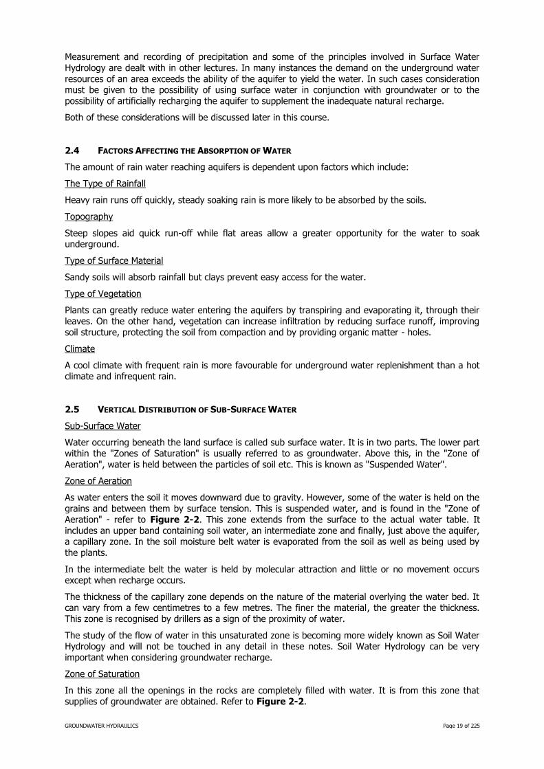
varying r ................................................................................................................83 Figure 6-8 Steady state flow example – semi-confined aquifer ..................................................91 Figure 6-9 Type curve solution, semi-confined aquifer, non-steady state ....................................95 Figure 6-10 Unconfined aquifer, steady state flow derivation ......................................................96 Figure 6-11 Steady state flow example – unconfined aquifer .......................................................99 Figure 6-12 Unconfined aquifer, variation of S with time ........................................................... 100 Figure 6-13 Delayed yield type curves ..................................................................................... 104 Figure 6-14 Boulton’s delay index curve .................................................................................. 108 Figure 6-15 Unconfined aquifer with delayed yield, non-steady state flow example .................... 109 Figure 6-16 Typical response curves for different aquifer types ................................................. 111 Figure 7-1 Constant drawdown example - straight line solution ............................................... 121 Figure 7-2 Constant drawdown test example using Eden-Hazel method ................................... 125 Figure 7-3 Step drawdown test – graphical analysis example .................................................. 133 Figure 7-4 Step drawdown test – graphical analysis, determination of “a” and “C” .................... 134 Figure 7-5 Step drawdown test – Eden-Hazel analysis............................................................. 138 Figure 7-6 Step drawdown test – Eden-Hazel analysis, determination of “a” and “C” ................ 139 Figure 7-7 Drawdown versus discharge curves for various times of discharge .......................... 142 Figure 7-8 Intermittent pumping – “F” versus “n” curves ........................................................ 146 Figure 7-9 Intermittent pumping – “F” versus “p” curves ........................................................ 147 Figure 7-10 Determination of long term pumping rate .............................................................. 150 Figure 8-1 Numerical analysis array ....................................................................................... 156 Figure 8-2 Numerical analysis example .................................................................................. 158 Figure 8-3 Typical flow net .................................................................................................... 159 Figure 8-4 Elemental square.................................................................................................. 160 Figure 8-5 Typical specific capacity - time - discharge curves .................................................. 163 Figure 9-1 Idealised section views of a discharging well in a semi-infinite aquifer bounded by a
perennial stream, and of the equivalent hydraulic system in an infinite aquifer ......... 172

GROUNDWATER HYDRAULICS TOC v
Figure 9-2 Generalised flow net showing stream lines and potential lines in the vicinity of a
discharging well dependent upon induced infiltration from a nearby stream ............. 173 Figure 9-3 Idealised section views of a discharging bore in a semi-infinite aquifer bounded by an
impermeable formation, and of the equivalent hydraulic system in an infinite aquifer174 Figure 9-4 Generalised flow net showing stream lines and potential lines in the vicinity of a
discharging well near an impermeable boundary .................................................... 175 Figure 9-5 Family of type curves for the solution of the modified Theis formula ........................ 177 Figure 10-1 Recharging pumped water to maintain water levels in sensitive areas...................... 187 Figure 10-2 Groundwater flow into a strip pit ........................................................................... 188 Figure 10-3 Multiple aquifer flow into a strip pit ....................................................................... 188 Figure 11-1 Constant discharge test – Callide Valley ................................................................. 192 Figure 11-2 Stable saltwater interface...................................................................................... 204 Figure 11-3 The dynamic saltwater interface ............................................................................ 207 Figure 11-4 Saltwater wedge in a confined aquifer ................................................................... 209 Figure 11-5 Saltwater wedge in an unconfined aquifer .............................................................. 211
TABLES
Table 1-1 Capillary rises in granular material ..............................................................................10 Table 1-2 Summary of the arithmetic mean of properties for all rock types ..................................14 Table 2-1 Distribution of sub-surface water ................................................................................20 Table 4-1 Indicative values of intrinsic permeability and hydraulic conductivity .............................34 Table 5-1 Recommended bore casing diameters (after Driscoll, 1986) .........................................42 Table 5-2 Suggested durations for discharge tests ......................................................................45 Table 5-3 Recommended pumping test applications ...................................................................54 Table 6-1 Data for steady state analysis ....................................................................................65 Table 6-2 Values of (Wu) for values of u between 10-15 and 9.9 ..................................................72 Table 6-3 Data for non-steady state flow analysis.......................................................................76 Table 6-4 Data for semi-confined aquifer test analysis ................................................................90 Table 6-5 Data for delayed yield analysis ................................................................................. 106 Table 7-1 G(α) for values of α between 10-4 and 1012 ............................................................... 115 Table 7-2 Richmond town bore no. 3 – test data ...................................................................... 118 Table 7-3 Format for pressure differential analysis ................................................................... 128 Table 7-4 Analysis of step drawdown test ................................................................................ 132 Table 7-5 Format for Eden-Hazel spreadsheet analysis ............................................................. 137 Table 7-6 Eden-Hazel test analysis .......................................................................................... 140 Table 7-7 Test data from Biloela, Callide Valley ........................................................................ 149 Table 7-8 Bore efficiencies for Richmond Town bore no. 3 ........................................................ 155 Table 7-9 Comparison of efficiency calculations ........................................................................ 155 Table 8-1 Average values of hydraulic conductivity of alluvial material in the Arkansas
Valley, Colorado ...................................................................................................... 165 Table 8-2 Storage coefficient approximation............................................................................. 165 Table 10-1 Drawdowns at control points during dewatering ........................................................ 187 Table 11-1 Pumping test data ................................................................................................... 191

GROUNDWATER HYDRAULICS Page 1 of 225
PREFACE
We have become accustomed to the belief that the most common source of useful water on our
planet is from rivers, streams, lakes and dams; a minor source is less obvious being underground. It is, however, extremely important. At any one time less than three percent of the available freshwater
on our planet is stored above ground, and more than 97% is stored below ground.
Surface water by virtue of its occurrence, is more easily understood. Groundwater, on the other hand,
because of its hidden nature, is shrouded with mystery and superstition.
Minor, though its use may be, it is extremely important, particularly in many parts of Australia where the annual rainfall is strongly seasonal, extremely variable and associated with very high evaporation,
and suitable surface water storage sites are not all that abundant.
The science of Groundwater Hydrology is concerned with the occurrence, availability and quality of
groundwater. Although many groundwater investigations are qualitative in nature, quantitative studies
are necessarily an integral part of the complete evaluation of occurrence and availability. The worth of an aquifer as a source of water depends largely on two inherent characteristics - its ability to store
water and to transmit water. As time progresses, its ability to mix waters of different qualities will also become more important.
There are very few places on this planet where one could drill a hole and not encounter water. In many cases, however, it may not be possible to extract water at a useful rate. The problem then is
not so much to locate groundwater, but to find a geologic formation which is capable of storing and
transmitting the water in useful quantities. Thorough knowledge of the geologic framework is essential before one can hope to understand the operation of the natural plumbing system within it.
Fortunately, most workers in the field of groundwater are geologists and geology will only be touched upon incidentally in these notes as it relates to some quantitative problem.
These notes give a brief coverage of the types of groundwater and the properties of water and water
bearing materials, but the main emphasis is on the hydraulic properties of the aquifers and the evaluation of groundwater systems.
The principal method of analysis in groundwater hydraulics is the application of equations derived for particular boundary conditions. These are generally applied to field tests of discharging bores. Prior to
1935, such equations were known only for the relatively simple steady-state flow conditions, which incidentally do not occur in nature. The development by Theis (1935) of an equation for the
non-steady state flow of groundwater was a milestone in groundwater hydraulics. Since 1935 the
number of equations and methods has grown rapidly and steadily. These are described in a wide assortment of publications, some of which are not conveniently available to many engaged in
groundwater studies. The essence of many of these will be presented and discussed, but frequent recourse should be made to the more exhaustive treatment given in the references cited. Indeed
many more papers have been written since these notes were first prepared and no attempt has been
made to include them.
In the years since 1973, when these notes were first prepared, the application of electronic computers
has simplified the solution of many difficult equations and computer programmes for most of the analyses presented in this document can be found on the internet. However, I would like to stress the
importance of knowing how the manual solutions are carried out before merely accepting the output
of a computer programme.
Also since 1973, groundwater modelling has developed significantly and is now used extensively for
the solution of many groundwater problems. However, it is very dangerous to attempt to build a groundwater model without a sound understanding of the physical properties and laws which control
groundwater storage and movement. When developing a groundwater model, carry out a rough check on the output. If the output is what you would expect and is based on reasonable physical parameters
of the aquifer material then use it to determine the temporal and spatial response of the aquifer to the
varying stresses placed upon it. If the output is not in accordance with what simple theory predicts or is only able to be calibrated by using unrealistic values for the aquifer parameters, then go back to the
drawing board and rebuild it.
To bring out the essential matters and relations and to give a better understanding of the applications
and of the limitations of the equations, worked examples and full derivations with their assumptions
have been included.

GROUNDWATER HYDRAULICS Page 2 of 225
In the limited time available I am able to present only a limited number of analytical methods.
However, a more complete coverage of the techniques available is presented in the extremely useful
reference "Analysis and Evaluation of Pumping Test Data" by G.P. Kruseman and N.A. de Ridder. The first edition of this reference was first published in 1970. A second edition was published in 1990.
In preparing these notes I have made use of both the above mentioned publication and of the lectures presented by S.W. Lohman to the Australian Water Resources Council Groundwater School,
1967.
I first prepared these notes in 1973 for presentation to the 4th Australian Water Resources Council Groundwater School which was held in Adelaide. They have been used extensively at many
Groundwater Schools since that time. I retyped and updated them slightly in 2009 but they are essentially the same as the original notes. I am grateful to the staff of Matrixplus Consulting for
formatting the document for me.
Apart from some additions for clarification, the only updates which I have included are minor and deal with flow through anisotropic media, a little more on the relationship between hydraulic conductivity
and intrinsic permeability and a brief introduction to the use of groundwater hydraulics in mine dewatering.
Colin P. Hazel
June 2009

GROUNDWATER HYDRAULICS Page 3 of 225
SECTION 1: PROPERTIES OF WATER AND WATER BEARING MATERIALS
1.1 INTRODUCTION
The science of Groundwater Hydrology is based upon the fundamental properties of firstly, water itself and secondly, the media through which it moves. At the risk of boring those people who have this basic knowledge at their fingertips, definitions and explanations of terms fundamental to this study are given here. If it serves no other purpose, this will at least collect the terms in a readily accessible place.
1.2 FLUID MECHANICS
It will be recalled that in the first consideration of solid objects they were assumed to be characterised by complete rigidity, i.e. by their ability to transmit shearing stresses.
Water, of course, is not a solid object (if frozen to ice it would be) but is a fluid and we define an ideal
fluid as a substance which is incapable of transmitting shearing stresses. Fluids can be divided into gases and liquids but we shall deal specifically with liquids.
The form or shape of any given mass of a liquid is quite indefinable as it conforms to the shape of the containing vessel. However, it does possess a definite volume at a definite temperature and pressure.
Liquids (particularly water) are but slightly compressible.
It is true that no real fluid can meet exactly the conditions of an ideal fluid since all fluids exert some
shearing stresses. For the moment we will, however, neglect this factor in our consideration of fluids
at rest.
1.2.1 Hydrostatics
Hydrostatics is simply the study of fluids at rest. The following definitions are applicable to fluids in general.
However, water is the fluid of prime concern, and the specific properties of water should be borne in
mind. Water is the only substance which can exist as solid, liquid or gas at atmospheric pressure.
Mass (or Inertia) (M) is the tendency of a body to resist a change of velocity. It determines the
acceleration of a body in response to a given force. Mass has often been explained in terms of "matter" but as the latter lacks any satisfactory definition, so then does the former in terms of it. Mass
is a fundamental, easily understood but not so easily adequately defined.
The unit of mass is the kilogram (kg).
Density (ξ) of a substance is its mass per unit volume. It varies with pressure and temperature.
ξ = M/V .....1.1
The unit of density is kilogram/cubic metre (kg/m3). The density of water at 4°C is 1000 kg/m3.
Densities at other temperatures from 0°C to 100°C are given in Figure 1-7.
Specific Gravity (S.G.) or Relative Density (R.D.) of a substance is the ratio of its density to the density
of water.
Being a ratio, it is dimensionless.
Displacement (s) is a change in position in a specified direction. It is then a vector quantity.
The unit of displacement is the metre (m).
Velocity (v) is the quantitative description of the motion of a body. Since it is related to direction as
well as speed of motion, it is a vector quantity. It is a rate of change of position in a specified
direction.
Instantaneous velocity = ds/dt
The units of velocity are metres per second (m/sec), or metres per day (m/day).
Acceleration (a) is the time rate of change of velocity, and is a vector quantity.
Instantaneous acceleration = dv/dt

GROUNDWATER HYDRAULICS Page 4 of 225
The units of acceleration are metres per second per second (m/sec2).
Acceleration due to gravity (g) is the acceleration produced on a body by the earth's gravitational field
and for most purposes is assumed to be constant at 9.80 m/sec2. It does, however, vary from place to place on the earth's surface.
Force (F) is that which produces or tends to produce a change in the state of motion of a body.
By Newton's second law of motion:
F = Ma
The force exerted on a body by the earth's gravitational attraction is referred to as its weight (W):
W = Mg .....1.2
The weight of a unit volume is referred to as the specific weight (γ):
γ = ξg
The adopted unit of force is the Newton, defined as that force which when acting on a mass of 1 kg
will produce an acceleration on it of 1 m/sec2.
A dyne is defined as the force required to move a mass of 1 gm with an acceleration of 1 cm/sec2.
The weight of a body having a mass of 1 kilogram is then 9.80 newtons (N).
Pressure (p) is defined as the perpendicular force per unit area exerted on a surface with which a fluid
is in contact.
The surface with which the fluid is in contact may, of course, be either a solid boundary or an
imaginary plane passed through the fluid for purposes of analysis.
p = F/A .....1.3
The adopted unit for pressure is the pascal (Pa), which is defined as 1 newton per square
metre (1 N/m). The common unit will be the kilopascal (kPa) which is 1000 pascals.
Strictly speaking, the magnitude of pressure should be expressed in terms of pascals above absolute
zero. However, it is generally more convenient to use atmospheric pressure as a reference, the
relative intensity p then representing the difference between absolute intensity pabs and atmosphere intensity pat.
i.e. p = pabs - pat .....1.4
Under normal conditions, pat = 101 kilopascals (kPa).
= 1010 millibars (mb) in meteorology.
Pressure may also be expressed in terms of the number of metres of water (or mercury) that a certain
pressure would support. Hydraulic head is measured in metres.
The pressure at a point A in a fluid h metres below the surface is given by:
p = pgh .....1.5
= a head of h metres of water
where:
p = pressure in pascals.
ξ = density in kg/m3.
h = depth in metres.
g = acceleration due to gravity = 9.8 m/sec2.
pat is then equal to a head 10.3 metres of water.
Pressure is the same at all points in the same horizontal plane within the fluid at rest. Any increment
of pressure applied at any point in a confined fluid is at once transmitted equally to all parts of the fluid.

GROUNDWATER HYDRAULICS Page 5 of 225
1.2.2 Hydrodynamics
Hydrodynamics is the study of fluids in motion.
This section deals with the motion of fluids and the various types of flow which may be encountered.
Steady Flow
Consider a fluid in motion in Figure 1-1 at a given time a particle of fluid at a given point, a, will have a particular velocity v1, at b a velocity v2, and at c at velocity v3. If, at all other times, the
velocity of whatever particle of fluid is at the point a, remains constant at v1, that at b remains v2 and
that at c remains v3, then the flow is said to be steady.
The path followed by a fluid particle in steady flow is called a streamline. Streamlines are
characterised by the property that the tangent at any point on the streamline gives the direction of flow of the fluid at that point. Particles of fluid may not flow from one streamline to another.
A bundle of similar streamlines is called a tube of flow e.g. steady flow in a pipe.
Non-Steady Flow
When the velocity of the particular fluid particle at a given point in a moving fluid varies with time, the
flow is described as non-steady.
Continuity Principle
Consider steady flow in a pipe of varying cross-sectional area as in Figure 1-2. Let the velocity of flow normal to plane A be v1 and at B be v2. Let the cross-sectional area of the pipe at A be A1, and at
B be A2.
Since the fluid is assumed to be incompressible the mass of fluid passing A in a given time t must equal the mass passing B in the same time, or there would be an accumulation of mass between A
and B, i.e. mass passing A in time t = mass passing B in time t:
v1 A1 t = v2 A2 t
or
v1A1 = v2A2 .....1.6
Figure 1-1 Steady flow
Figure 1-2 Continuity principle

GROUNDWATER HYDRAULICS Page 6 of 225
Thus in the case of steady flow in a pipe of varying cross-section, the highest velocity occurs at the
smallest section.
Since the fluid undergoes an acceleration in moving from A to B, from the second law of motion (F = Ma) the pressure at A must be higher than the pressure at B.
This principle is used in the venturi which is used to measure flows in pipes. Small tubes tapped into a constricted pipe at positions such as A and B enable the difference in pressure to be recorded. This
pressure difference is proportional to the velocity squared, so the meter can be calibrated to read flow
directly.
Bernoulli's Theorem
By the application of the principle of conservation of energy to the flow of a fluid in a tube of flow, Bernoulli's Theorem can be derived, viz:
.....1.7
or is sometimes written:
.....1.8
where:
p = pressure.
ξ = density of fluid.
g = acceleration due to gravity.
v = velocity.
h = potential or elevation head above datum level.
hf = head lost in overcoming friction when the fluid moves from the point 1 to point 2.
It must be emphasised that Bernoulli's Theorem is strictly applicable only to streamline flow.
In equation 1.7:
p/ξg = the pressure head.
v2/2g = the velocity head.
h = the elevation head.
The total head at any point is the summation of these three terms.
The summation of the elevation head and pressure head gives the potentiometric head, and the
concept is useful in analysing flows in pipes and flow in underground water.
A popular misconception is that flow takes place from areas of high pressure to areas of low pressure. This is not so. Flow occurs from areas of high potentiometric head to areas of low potentiometric
head. With a suitable arrangement of elevation heads it is possible for a fluid to flow from an area of low pressure to one of high pressure, e.g. the pressure in a storage tank located on a hill is smaller
than the pressure in a pipeline some distance down the hill. However, because of the greater
elevation on the hill, the potentiometric head is greater at the tank site and water is delivered along the pipe.
Viscosity
So far, only "ideal fluids" have been considered, i.e. fluids which cannot transmit shearing stresses
and on which no work is done in changing their shape.
In actual fact, no fluid is ideal and all possess, to some degree, the property of viscosity or internal friction.
The coefficient of dynamic viscosity or absolute viscosity (ε) is defined as the ratio of the intensity of shear, η, to the rate of deformation.
ttanconshg
v
g
p
2
2
fhhg
v
g
ph
g
v
g
p2
2
221
2
11
22

GROUNDWATER HYDRAULICS Page 7 of 225
i.e. .....1.9
where:
ε = dynamic viscosity.
η = intensity of shear.
dv/dy = velocity gradient in the transverse direction.
Figure 1-3 Dynamic viscosity
If we consider two plates in Figure 1-3 of surface area A separated by a thickness y of fluid and
moving at a velocity v relative to each other under an imposed force F, then:
.....1.10
where:
F = total tangential force applied, (N).
A = Area over which the force is applied, (m2).
ε = coefficient of dynamic viscosity, in decapoises (Nsm-2).
v = relative velocity, (m/sec).
y = distance between the layers at which velocity is measured, (m).
The coefficient of dynamic viscosity depends on the fluid and on its temperature.
In terms of units:
ε =
ε will have the dimensions of newton second/m2 and the unit is known as the decapoise.
Another viscosity coefficient, the kinematic coefficient of viscosity is defined by:
Kinematic coefficient of viscosity .....1.11
Laminar and Turbulent Flow
In laminar flow, the fluid particles move along parallel paths in layers or laminae. The magnitudes of
the velocities of adjacent laminae are not necessarily the same. Laminar flow is governed by the equation given as the definition of dynamic viscosity above, i.e.
.....1.12
The viscosity of the fluid is dominant and thus suppresses any tendency towards turbulence.
Above a certain critical velocity, the viscosity of the fluid is insufficient to damp out turbulence and the fluid particles move in a haphazard fashion where it is impossible to trace the motion of an individual
particle. Such motion is called turbulent flow.
y
F v
Fluid
dydv /
v
y
A
F.
)/(
)(
)(
)(2 secmvelocity
mcetandisx
marea
newtonsforce
)(.
)(cos.
densitymass
ityvisabsolute
dy
dv

GROUNDWATER HYDRAULICS Page 8 of 225
The shear stress for turbulent flow can be expressed as:
dy
dvz)(
.....1.13
where z is a factor depending on the density of the fluid and the fluid motion.
Reynold's Number
In pipeflow the transition from laminar to turbulent flow is characterised by well known values of
Reynold's Number (NR) which expresses the ratio of the inertial to viscous forces. Thus, there is a
lower limit critical number around 2100 below which flow in pipes is always laminar.
By analogy, in flow through porous media a Reynold's Number has been established as:
.....1.14
where:
v = the specific discharge, i.e. discharge per unit area.
D = a characteristic length. In pipe flow D is the internal diameter of the pipe. In flow
through porous media D is related to grain size.
= the kinematic viscosity of the fluid.
Because the grain sizes are so variable in flow through porous media no one value for Reynold's
Number can be set as the dividing line between laminar flow and turbulent flow. It has been
established that this transition occurs normally for a Reynold's Number in the range 1 to 10.
For non-circular cross-sections (in open channel flow):
where R is the hydraulic radius, and is equal to the ratio of the cross-sectional area to the wetted
perimeter.
Surface Tension (ζ)
Surface Tension is a property associated with the free surface of any liquid or the interface between any two non-miscible liquids.
It is well known that many insects are able to walk on the surface of liquids in apparent contradiction
to Archimedes' Principle. This property tends to suggest that there is a kind of membrane or skin that envelopes all liquids. In fact this very nearly describes what actually the situation is.
A molecule in the interior of a fluid is acted upon by attractive forces in all directions and the vector sum of these is zero. However, at the surface, a molecule is acted upon by a net inward cohesive
force perpendicular to the surface. Hence work is required to bring molecules to the surface.
The surface tension of a liquid is the work that must be done to bring enough molecules from inside
the liquid to form one new unit area on the surface.
The intermolecular forces also come into play when a liquid is in contact with a solid object - in this case there is an attraction of the molecules of the solid for those of the liquid.
Hence, for example, if pure water is placed in a clean glass container it will be observed that the water surface in contact with the glass turns up and lies flat on the glass. Thus the attraction of glass
for water is greater than that of water for itself.
On the other hand mercury placed in a glass container will be observed at the surface contact, to be drawn away from the glass indicating that the attraction of glass for mercury is less than that of
mercury for itself.
Capillarity or the rise or fall of a liquid in a capillary tube is caused by surface tension and depends on
the relative magnitudes of the cohesion of the liquid and the adhesion of the liquid to the walls of the containing vessel. Liquids rise in tubes they wet (adhesion > cohesion) and fall in tubes they do not
wet (cohesion > adhesion).
vDNR
)4( RvNR

GROUNDWATER HYDRAULICS Page 9 of 225
Figure 1-4 Capillary rise
From Figure 1-4:
cos22 rghr c .....1.15
cos2
grhc
.....1.16
where:
r = radius of the tube (m).
ξ = density of the fluid (kg/m3).
g = gravitational acceleration (9.8 m/sec2).
ζ = surface tension (newtons/m).
hc = capillary rise (m).
α= angle of contact between solid liquid and gas.
For pure water in clean glass:
α = 0 and cos α = 1
At 20˚C:
ζ = 0.073 N/m
ξ = 1000 kg/m3
hence:
hc = 1.5/r x 10-5 m .....1.17
where:
hc = capillary rise in metres.
r = radius of tube in metres.
Surface Tension is dependent on temperature; so then is capillarity.
At 99°C, for pure water in a clean glass:
ζ = 0.0591 N/m
ξ = 959 kg/m3
hc = (1.26/r) x 10-5
α
2r
hc p < atmospheric
p = atmospheric
density ξ, surface tension ζ

GROUNDWATER HYDRAULICS Page 10 of 225
Capillary rise in granular material is comparable to a bundle of capillary tubes of various diameters,
see Figure 1-5.
Figure 1-5 Capillary rise in tubes
Capillary rises in samples having essentially the same porosity (41%) after 72 days (Atterberg, cited in
Terzaghi, 1942) are given in Table 1-1. (Note that hc is nearly inversely proportional to grain size).
Table 1-1 Capillary rises in granular material
Material Grain Size (mm) hc (cm)
Fine Gravel 5 - 2 2.5
Very Coarse Sand 2 - 1 6.5
Coarse sand 1 - 0.5 13.5
Medium Sand 0.5 - 0.2 24.6
Fine Sand 0.2 - 0.1 42.8
Silt 0.1 - 0.05 105.5
Silt 0.05 - 0.02 *200
* Still rising after 72 days
1.3 SOIL MECHANICS
This study of Soil Mechanics will be limited to those soil properties relevant to groundwater hydraulics.
In general then, the study will be limited to porous media. Porous media are comprised of two distinct parts, a granular matrix and interconnected voids. In a saturated porous medium, water (or some
fluid) fills all of the voids or pore spaces.
1.3.1 Grain-Void Relationship
Porosity (ζ) of the soil mass is defined as the ratio of volume of the voids to the total volume of the
mass:
ζ= Vv/VT .....1.18
where:
Vv = volume of voids
VT = total volume
Primary porosity is related to granular material, while secondary porosity refers to the opening in joints and faults in hard rocks, and solution openings in limestone, dolomite, gypsum or other soluble
rocks.
Porosity is commonly expressed as a percentage and has no units.

GROUNDWATER HYDRAULICS Page 11 of 225
The porosity of a soil obviously depends on the properties of its constituent grains, some of which are
enumerated below.
Shape of the grains: since porosity is a function of the volume of voids, the more intimate the contact between grains the lower the porosity. Angularity tends to increase porosity.
Size of grains: provided grain size is uniform, the actual size will have no effect on the porosity.
Degree of assortment: a wide range of grain sizes will result in a smaller volume of voids and hence a
lower porosity. On the other hand, uniform sized grains will produce a higher porosity.
Type of packing or arrangement of grains: consider the idealized case of uniform sized spherical grains. For square packing a porosity of 47.64% is achieved, while for rhombic packing the porosity
will be only 25.95%.
In the same way, for random size and shape of grains, the porosity is controlled by the packing c.f.
maximum and minimum density.
Voids Ratio (e) is defined as the ratio of the volume of the voids to the volume of solids.
e = Vv/Vs .....1.19
1.3.2 Fluid Flow Properties
Coefficient of Permeability or Hydraulic Conductivity (K)
The law governing laminar water flow through soils is Darcy's Law and may be expressed as:- (See Section 4).
Q = -KiA .....1.20
where:
Q = rate of flow (in cubic metres per day).
i = hydraulic gradient or head loss per unit distance travelled (non dimensional).
A = the cross-sectional area through which the flow occurs (in square metres).
K = the coefficient of permeability or hydraulic conductivity (in metres/day).
The coefficient of permeability should not be confused with intrinsic permeability (See Section 4).
Darcy's Law may also be written:
KivA
Q
.....1.21
However careful distinction must be made between the superficial velocity v and the actual seepage
velocity vs where:
Q = Av = Av Vs .....1.22
where:
Q = total discharge rate.
A = cross-sectional area of porous medium.
v = average discharge velocity.
Av = cross-sectional area of voids.
Vs = actual seepage velocity.
Hence:
v = ζ vs .....1.23
where:
ζ = porosity.

GROUNDWATER HYDRAULICS Page 12 of 225
Hydraulic Conductivity may be determined in the laboratory by the use of permeameters or in the field
by pumping tests. Because of the problems associated with obtaining undisturbed samples and of
repacking disturbed samples in the laboratory, coefficients of permeability obtained from laboratory tests must be considered unreliable.
In practice, most aquifers are non-homogeneous and anisotropic (i.e. the material does not have like properties on all orientations of planes, generally resulting from stratification) and the hydraulic
conductivity will vary with location and direction of flow. The aquifer characteristics obtained from
pumping tests represent the average of values around the discharging bore.
Hydraulic conductivity and porosity are essentially unrelated e.g. clay generally has a high porosity
and low hydraulic conductivity while sand has a low porosity but high hydraulic conductivity.
Intrinsic Permeability (k)
The velocity of laminar flow through a porous medium may be described almost exactly by the
equation:
.....1.24
where:
ip = the pressure gradient.
ε = the dynamic viscosity of the fluid.
k = the intrinsic permeability (square micrometre).
This may be written:
gikv
.....1.25
where:
i = hydraulic gradient.
This equation is of the same form as the Darcy equation:
v = Ki
Hence:
.....1.26
The intrinsic permeability (k) is related solely to the properties of the porous medium. The coefficient of permeability or hydraulic conductivity (K) is related not only to the properties of the porous medium
but also to the properties of the fluid.
From extensive laboratory testing, Hazen found that the coefficient of permeability of sands in a loose
state depended on two quantities he called the effective grain size and the uniformity coefficient.
The effective grain size D10 of a sample is a grain size diameter such that 10 percent of the particles
are finer and 90 percent coarser.
Dn is defined as that diameter such that n% of the particles in a sample are finer.
The uniformity coefficient U is defined as:
10
60
D
DU
.....1.27
1.3.3 Soil Pressures
Pore Water Pressure
If the pores or interstices of a porous medium are filled with water then this water is subject to the same principles as outlined in section 1.1.1, hydrostatics.
pikv
kggkK

GROUNDWATER HYDRAULICS Page 13 of 225
The hydrostatic pressure in the water is given by:
pw = ξgh .....1.28
where:
pw = hydrostatic or pore water pressure.
ξ = density.
g = gravitational acceleration.
h = depth below the potentiometric level.
Intergranular Pressure
If a load is applied to an unsaturated porous medium it is transmitted from grain to grain at the points
of contact. The pressure at the points of contact, i.e. the intergranular pressure, is dependent on the force applied and the area of contact. The application of a force results in a larger area of
intergranular contact with a resultant slight deformation of the matrix and a reduction in voids ratio.
Total Pressure
If the porous medium is saturated and a confining layer placed over its surface and a load is applied,
see Figure 1-6, then the load is taken partly by the pore water and partly by the grains.
Figure 1-6 Pressure distribution
If the total pressure applied to the porous medium, i.e. force/area, is pt then at the interface of the
porous medium and confining layer:
pt = pw +pg .....1.29
where:
pt = total pressure.
pw = that part of the pressure borne by water (pore water pressure).
pg = that part of the pressure borne by grains.
When the applied load is in fact the material overlying an aquifer, then changes in applied load such
as atmospheric pressure changes or tidal changes will result in changes in pore water pressure with resultant changes in potentiometric level.
Likewise, a lowering of the potentiometric level by pumping results in a lowering of the pore water
pressure and a resultant increase in load to be carried by the grains and a slight compression of the aquifer matrix. An understanding of this transfer of pressures is necessary if the concept of storage
coefficient is to be understood.
1.3.4 Properties of Rock Types
The Hydrologic Laboratory of the U.S.G.S. has conducted tests on number of samples in order to
determine their properties. Table 1-2 summarises the arithmetic mean of properties determined by these tests. It must be stressed that the values are only indicative.
The table is taken from "Summary of Hydrologic and Physical Properties of Rock and Soil Materials as Analysed by the Hydrologic Laboratory of the U.S.G.S., 1948 - 1960".

GROUNDWATER HYDRAULICS Page 14 of 225
Table 1-2 Summary of the arithmetic mean of properties for all rock types
Strata
Property
Hydraulic Conductivity Dry Unit Weight (g/cc)
S.G. of Solids
Porosity Undisturbed
(%)
Porosity Repack
(%)
Specific Retention
(%)
Specific Yield (%) Repack
(m/day) Vert.
(m/day) Horiz.
(m/day)
Sedimentary Rocks
Water-Laid Deposits
Sandstone Fine 0.2 0.29 1.76 2.65 33 13 21
Medium 3.1 1.68 2.66 37 10 27
Siltstone N 1.61 2.65 35 43 29 12
Claystone N 1.51 2.66 43
Shale 2.53 2.73 6
Clay N N 1.49 2.67 42 48 38 6
Silt 0.0025 0.08 1.38 2.66 46 46 28 20
Sand Fine 2.5 3.8 1.55 2.67 43 32 8 33
Medium 12 14 1.69 2.66 39 35 4 32
Coarse 45 28 1.73 2.65 39 34 5 30
Gravel Fine 450 1.76 2.68 34 7 29
Medium 273 1.85 2.71 32 7 24
Coarse 150 1.93 2.69 28 9 21
Wind-Laid Deposits
Loess 0.08 1.45 2.67 49 46 27 18
Aeolian Sand 20 1.58 2.66 45 38 3 38
Tuff 0.16 1.48 2.50 41 21 21
Ice Laid Deposits
Till Clay 2.65
Silt 1.78 2.70 34 28 6
Sand 0.5 1 1.88 2.69 31 14 16
Gravel 30 1.91 2.72 26 12 16
Washed Silt 0.2 1.38 2.72 49 9 40
Drift Sand 38 14 1.55 2.69 44 36 3 41
Gravel 204 1.60 2.68 39 41

GROUNDWATER HYDRAULICS Page 15 of 225
Strata
Property
Hydraulic Conductivity Dry Unit Weight (g/cc)
S.G. of Solids
Porosity Undisturbed
(%)
Porosity Repack
(%)
Specific Retention
(%)
Specific Yield (%) Repack
(m/day) Vert.
(m/day) Horiz.
(m/day)
Sedimentary Rocks (continued)
Chemical and Organic Deposits
Limestone 1 1.8 1.94 2.75 30 13 14
Dolomite 2.02 2.69 26
Peat 5.7 0.13 1.54 92 49 44
Igneous Rocks
Weathered Granite 1.4 1.50 2.74 45
Weathered Gabbro 0.16 1.73 3.02 43
Basalt 0.008 2.53 3.07 17
Metamorphic Rocks
Schist 0.16 1.76 2.79 38 17 26
Slate N 2.94
Note: N indicates Negligible

GROUNDWATER HYDRAULICS Page 16 of 225
Figure 1-7 Properties of pure water

GROUNDWATER HYDRAULICS Page 17 of 225
SECTION 2: OCCURRENCE OF GROUNDWATER
2.1 INTRODUCTION
Natural underground reservoirs have many advantages. They are freely available for storing water without construction expenditure. Commonly, they have enormous capacities and do not become
clogged with silt and weeds as do lakes and reservoirs. They are relatively inexpensive to tap; they lose little or no water by evaporation; they can supply water over very large areas without the
necessity of building channels, pipelines or other distribution systems; and, if properly managed, their
period of usefulness has no foreseeable limit.
Groundwater occurs in the pores and interstices of rocks. In semi-confined aquifers (Section 3) large
volumes of water may be stored in the semi-pervious layers above and/or below the main aquifer. With a reduction in pressure this water moves vertically to the aquifer which then transmits it to the
bore.
The volume stored in any saturated material is given by:
.....2.1
And the volume released under gravity drainage is given by:
.....2.2
where:
Vv = volume of stored water (also volume of interstices).
VT = total volume of saturated material.
VD = volume of water released by gravity drainage.
ζ = porosity.
Sy = specific yield.
2.2 ORIGIN OF GROUNDWATER
Groundwater may originate in any of three ways:
Juvenile Water has its origin in molten rocks which underlie the earth's crust at great depths. These
rocks sometimes find their way to the surface, or near surface, of the earth. Upon cooling of the rock, water may be trapped or given off as steam from a volcanic vent. From the point of view of
worthwhile supplies of groundwater, juvenile water has little or no significance.
Connate Water is water trapped in the interstices of a sedimentary rock at the time it was deposited.
It may, for example, have been derived from the ocean or from fresh water sources, depending on
the locality in which the sedimentary rock was formed. Although of little importance from the point of view of significant quantities of groundwater being obtained from this source, it is nevertheless most
important in its effect on water quality in various rocks.
Meteoric Water is water derived from the atmosphere, generally in the form of rain and sometimes
snow and hail. It is the basic source from which the great bulk of groundwater is derived.
2.3 HYDROLOGIC CYCLE
The earth's water supplies are being constantly circulated. Figure 2-1 illustrates this cycle. The sun's heat evaporates water from the seas and lakes covering two-thirds of the earth's surface. This
evaporated water is virtually free of saline matter. The moisture forms clouds which precipitate as rain
over both the sea and land.
Tv VV
yTD SVV

GROUNDWATER HYDRAULICS Page 18 of 225
Some is evaporated before reaching the ground; more is intercepted by plant life and returned to the
atmosphere. Some rain which reaches the land surface makes its way back to the sea through rivers
and lakes. In doing so, it is subject to further evaporation. Some rain finds its way underground and this is the major source of water underground. Part of this water which has entered the soil is used by
plant life, and returns to the atmosphere through leaves. However, a proportion does eventually penetrate deep underground and is stored in natural materials. Even this water is acted upon by
gravity, and in the long term tends to make its way back to the sea to help recommence the cycle.
Figure 2-1 Hydrologic cycle
GROUNDWATER HYDRAULICS Page 19 of 225
Measurement and recording of precipitation and some of the principles involved in Surface Water
Hydrology are dealt with in other lectures. In many instances the demand on the underground water
resources of an area exceeds the ability of the aquifer to yield the water. In such cases consideration must be given to the possibility of using surface water in conjunction with groundwater or to the
possibility of artificially recharging the aquifer to supplement the inadequate natural recharge.
Both of these considerations will be discussed later in this course.
2.4 FACTORS AFFECTING THE ABSORPTION OF WATER
The amount of rain water reaching aquifers is dependent upon factors which include:
The Type of Rainfall
Heavy rain runs off quickly, steady soaking rain is more likely to be absorbed by the soils.
Topography
Steep slopes aid quick run-off while flat areas allow a greater opportunity for the water to soak underground.
Type of Surface Material
Sandy soils will absorb rainfall but clays prevent easy access for the water.
Type of Vegetation
Plants can greatly reduce water entering the aquifers by transpiring and evaporating it, through their
leaves. On the other hand, vegetation can increase infiltration by reducing surface runoff, improving
soil structure, protecting the soil from compaction and by providing organic matter - holes.
Climate
A cool climate with frequent rain is more favourable for underground water replenishment than a hot climate and infrequent rain.
2.5 VERTICAL DISTRIBUTION OF SUB-SURFACE WATER
Sub-Surface Water
Water occurring beneath the land surface is called sub surface water. It is in two parts. The lower part within the "Zones of Saturation" is usually referred to as groundwater. Above this, in the "Zone of
Aeration", water is held between the particles of soil etc. This is known as "Suspended Water".
Zone of Aeration
As water enters the soil it moves downward due to gravity. However, some of the water is held on the
grains and between them by surface tension. This is suspended water, and is found in the "Zone of Aeration" - refer to Figure 2-2. This zone extends from the surface to the actual water table. It
includes an upper band containing soil water, an intermediate zone and finally, just above the aquifer, a capillary zone. In the soil moisture belt water is evaporated from the soil as well as being used by
the plants.
In the intermediate belt the water is held by molecular attraction and little or no movement occurs except when recharge occurs.
The thickness of the capillary zone depends on the nature of the material overlying the water bed. It can vary from a few centimetres to a few metres. The finer the material, the greater the thickness.
This zone is recognised by drillers as a sign of the proximity of water.
The study of the flow of water in this unsaturated zone is becoming more widely known as Soil Water Hydrology and will not be touched in any detail in these notes. Soil Water Hydrology can be very
important when considering groundwater recharge.
Zone of Saturation
In this zone all the openings in the rocks are completely filled with water. It is from this zone that supplies of groundwater are obtained. Refer to Figure 2-2.

GROUNDWATER HYDRAULICS Page 20 of 225
Figure 2-2 Vertical distribution of sub-surface water
In non-pressure or unconfined aquifers, the top of the zone is called the water table. The water table
will fluctuate with recharge, use and groundwater flow.
In confined aquifers the water is prevented from rising by a confining layer. If a number of bores were
drilled through this confining layer the heights to which the water would rise would represent the potentiometric surface of the aquifer.
For the most part the presence of groundwater is continuous in the zone of saturation. However, its
availability depends upon the nature of the rock formation in which it occurs. For example, clay may be saturated but will not release the water to a bore or well. On the other hand, coarse saturated
gravel would yield large quantities.
In some cases the rate at which the saturated material will yield water is so slow that it is not
immediately obvious in a well or bore and drillers are inclined to say that the hole is dry.
This can explain the situation where a bore is drilled a few feet from a so called dry hole and yields a substantial quantity of water. In actual fact in both cases the material may be saturated but only
in the latter case will it yield water at a rate sufficient to give a successful bore.
The schematic representation in Table 2-1 gives the complete range of divisions. These will all be
present in areas of relatively deep water tables after prolonged dry spells. In other areas with higher water tables the uppermost divisions may not be present. Beneath lakes, swamps and
streams only the zone of saturation will be present.
Table 2-1 Distribution of sub-surface water
Pressure Zone Division(1) Bore
Gas phase, equals atmospheric
Unsaturated Zone Discontinuous capillary saturation
Liquid phase, less than atmospheric
Semi-continuous capillary saturation
Less than atmospheric
Saturated(2) Zone Continuous capillary saturation
Atmospheric water table S.W.L.
Greater than atmospheric Unconfined aquifer
Notes: (1) Capillary "Zones" of Terzaghi (1942)
(2) As redefined by Hubbert (1940). See also Lohman (1965, p.92).
Bedrock
Groundwater
Capillary Water
Soil Water
Soil Water Zone
Intermediate Zone
Capillary Zone
Suspended Water
Zone of Saturation
Zone of Aeration

GROUNDWATER HYDRAULICS Page 21 of 225
SECTION 3: AQUIFERS
3.1 DEFINITIONS
Aquifer
Lohman and others 1972, have defined an aquifer as a formation, group of formations or part of a
formation that contains sufficient saturated permeable material to yield significant quantities of water to bores and springs. Under this definition, an aquifer includes both the saturated and unsaturated
part of the permeable formation.
Confined (or Pressure or Artesian) Aquifer
A confined aquifer is a completely saturated permeable formation of which the upper and lower
boundaries are impervious layers. Completely impervious layers rarely exist in nature and hence confined aquifers are less common than is often realised.
In a confined aquifer the water is under sufficient pressure to cause it to rise above the aquifer if
given the opportunity e.g. if penetrated by a bore. The level to which the water rises is called the potentiometric level, the standing water level (S.W.L.) or static head. Pressure water or confined
water relates to water contained in aquifers of this nature.
If the pressure is sufficient to raise the water to the surface when a bore penetrates such an aquifer
then the water may flow from the bore without mechanical assistance. This type of bore is called a "flowing artesian bore".
Unconfined (Non Pressure or Water Table) Aquifer
An unconfined aquifer is a permeable formation only partly filled with water and overlying a relatively impervious layer.
It contains water which is not subjected to any pressure other than its own weight. If a bore penetrates such an aquifer the water will rise up the bore no higher than the depth at which it was
first encountered.
The level at which water stands in a bore penetrating an unconfined aquifer, i.e. the standing water level, is known as the water table, and is the depth at which the water in the unconfined aquifer is at
atmospheric pressure. Water does occur in the aquifer above the water table but at pressures less than atmospheric.
A perched aquifer is an unconfined aquifer separated from an underlying body of groundwater by an unsaturated zone. Its water table is a perched water table. It is supported by a perching bed whose
permeability is low. Perched groundwater may be either permanent or temporary.
Water in an unconfined aquifer is called unconfined or phreatic water.
Semi-Confined (or Leaky) Aquifer
The confining layers of many pressure aquifers are not completely impervious. The hydraulic conductivity of the confining layer may be very small when compared with that of the aquifer material,
but as the radius of influence of a discharging facility increases, the area through which the confining
layer is contributing water becomes very large and the volume of water contributed can be a very significant part of the total water discharged.
Such an aquifer is called a leaky or semi-confined aquifer. The flow of water from the confining layer to the aquifer is assumed to be vertical. The horizontal movement in this layer is negligible.
Semi-Unconfined Aquifer
If the hydraulic conductivity of the fine grained layer in a semi-confined aquifer is so great that the horizontal flow component in the covering layer cannot be ignored, then such an aquifer is
intermediate between the semi-confined aquifer and the unconfined aquifer and may be called a semi-unconfined aquifer.
In general, such aquifers do not release their water instantaneously from storage and exhibit what is called delayed drainage. Such aquifers may be called unconfined aquifers exhibiting delayed drainage
or delayed yield effects.
Schematic representation of the aquifer types is given in Figure 3-1.

GROUNDWATER HYDRAULICS Page 22 of 225
Figure 3-1 Aquifer types
Aquiclude
An aquiclude is an impermeable formation which may contain water, but is incapable of transmitting it
in quantities large enough to warrant extraction by a well or a bore.
Aquifuge
An aquifuge is an impermeable formation which neither contains nor transmits water. An example of
an aquifuge is solid granite.
Confining Bed
U.S.G.S. Water Supply Paper 1988 suggests that the term "confining bed" should supplant the terms
"aquiclude", "aquitard" and "aquifuge". It is a body of impermeable material stratigraphically adjacent to one or more aquifers.
Homogeneous and Isotropic
Two other terms which are frequently used in groundwater hydraulics are "homogeneous" and
"isotropic". Homogeneous means "the same at all locations" and isotropic means "the same in all directions".
The drilling logs of bores drilled anywhere in a homogeneous aquifer would be identical both in
material encountered and the thickness of material even though a number of different rock types was encountered throughout the depth of the bore.
In a non-homogeneous aquifer the material encountered and the thickness of material could both vary from place to place in the aquifer.
In an isotropic aquifer the type of material and its properties are the same in all directions. In nature,
aquifer material has been laid down in such a way that properties vary in different directions e.g. it is normally easier for water to move along the direction of layering in a horizontal direction than it is to
move across layers in a vertical direction.

GROUNDWATER HYDRAULICS Page 23 of 225
3.2 AQUIFER FUNCTIONS
An aquifer has three important functions namely:
Storage
It stores water as a reservoir. The aquifer characteristic describing the ability of an aquifer to store
water is the Porosity. The characteristic describing its ability to release water under gravity drainage is its specific yield. The property describing its elastic storage is the Storage Coefficient or Storativity,
and this is related to the elastic properties of both the water and aquifer material.
Transmission
It transmits water like a pipeline. The relevant aquifer characteristics are Hydraulic Conductivity and
Transmissivity (called Transmissibility in some references).
Mixing
It mixes water of different qualities. Poor quality water can be injected into an aquifer at one point,
mixed with the local groundwater and the mixture withdrawn as useable water at another location.
3.3 TYPES OF AQUIFER FORMATIONS
There are two general classes of formation which store and transmit water. These are:
Porous Rocks
Spaces between grains of sand and gravel - unconsolidated sands and gravels and consolidated
sandstones;
Fractured Rocks
These include crevices, joints and fractures in hard rock; and solution channels in limestone, and
shrinkage cracks and gas bubbles in basalt type volcanic rocks.
3.4 HYDRAULIC PROPERTIES
There are ten main hydraulic properties of the aquifer which should be understood. These are:
1. Hydraulic Conductivity.
2. Transmissivity.
3. Storage Coefficient.
4. Specific Mass Storativity.
5. Specific Yield.
6. Specific Retention.
7. Hydraulic Resistance.
8. Leakage Coefficient.
9. Leakage Factor.
10. Drainage Factor.
Hydraulic Conductivity (K) (see also Sections 1 and 4)
The hydraulic conductivity of an aquifer is the rate at which water at the prevailing viscosity can be transmitted through a unit area of an aquifer, normal to the direction of flow, under a unit gradient. It
is sometimes referred to in engineering literature as the coefficient of permeability.
.....3.1
where:
q = discharge rate per unit area normal to the direction of flow.
i = hydraulic gradient.
i
qK

GROUNDWATER HYDRAULICS Page 24 of 225
Hydraulic conductivity is dependent primarily on the nature of the pore space, the type of liquid
occupying it, and the gravitation attraction.
In a layered anisotropic aquifer the hydraulic conductivity will be different from layer to layer and the average hydraulic conductivity for the aquifer will be a function of the individual hydraulic
conductivities of each layer. In addition, the hydraulic conductivity is normally greater along the layering than across it and also greater along the direction of flow for extrusive igneous rocks. Hence,
the hydraulic conductivity is generally much greater in the horizontal direction than in the vertical
direction. In the absence of more precise data it can be assumed that the horizontal hydraulic conductivity is an order of magnitude greater than the vertical.
Figure 3-2 Homogeneous anisotropic formation
In Figure 3-2, the anisotropic formation comprises 3 layers of thicknesses b1, b2, and b3 with
hydraulic conductivities K1, K2 and K3 respectively.
The average horizontal hydraulic conductivity of a formation with n layers is given by:
.....3.2
where:
Khav = average horizontal hydraulic conductivity.
Khm = the hydraulic conductivity of the mth layer.
bm = the thickness of the mth layer.
b = the total thickness of the aquifer.
The effective hydraulic conductivity for vertical flow i.e. for flow through the n layers in the y direction
is given by:
.....3.3
where:
Kveff = the effective hydraulic conductivity for vertical flow.
Kvm = the vertical hydraulic conductivity of the mth layer.
bm = the thickness of the mth layer.
b = the total thickness of the aquifer.
Equations 3.2 and 3.3 are analogous to the flow of electricity through a series of resistors. In equation 3.2 the resistors are in parallel and in equation 3.3 the resistors are in series.
The dimensions of hydraulic conductivity are Volume/time/area (Length/Time). The units to be used
are m/day or m3/day/m.
K1
K2
K3
b1
b2
b3
b
y
x
b
bKavK mhmn
mh 1
vm
mn
m
v
K
b
beffK
1

GROUNDWATER HYDRAULICS Page 25 of 225
Transmissivity (T)
The transmissivity of an aquifer is the rate at which water at the prevailing viscosity can be
transmitted through a unit strip of aquifer under a unit gradient.
T= Kb .....3.4
where
K = the hydraulic conductivity.
b = aquifer thickness.
The dimensions of transmissivity are Volume/unit time/unit width (Length2/Time). The units to be used are m/day/m or m/day.
Storage Coefficient (S) (Confined Aquifers)
The storage coefficient or storativity of an aquifer is defined as the volume of water which a saturated
column of aquifer releases from or takes into storage per unit surface area per unit change in head.
Storage coefficient is related to the elastic properties of the water and of the soil matrix. It is not an indication of the total volume stored in an aquifer.
For a confined aquifer the value of Storage Coefficient ranges from about 10-5 to 10-3 or about 5 x 10⁻⁶ per metre of aquifer thickness.
C.E. Jacob (1940, 1950), probably the first to consider flow in an elastic aquifer, derived the equation for Storage Coefficient as:
.....3.5
where:
b = thickness of the aquifer.
ξ = density of the fluid (for water = 1,000 kg/m3).
g = acceleration due to gravity.
ζ = porosity.
β = compressibility of water, 4.8 x 10⁻⁷ kPa i.e.4.8 x 10-10 m2/N.
Ew = 1/β bulk modulus of water 2.08 x 10⁶ kPa.
α = compressibility of soil matrix. Sand and gravel α ~ 10-8 m2/N
Es = 1/α = bulk modulus of soil matrix.
C = a dimensionless ratio, which may be considered unity in an uncemented granular material. In a solid aquifer such as limestone having tubular solution cavities, C is apparently
equal to the porosity. The value for a sandstone ranges between these limits, depending upon the degree of cementation.
Bear (1972, p.207), suggests that the above expression is in error and the correct expression for
porous media should be:
))1((gbS
.....3.6
Bear's approach considers a constant control volume with both the fluid and soil matrix being free to
move across the boundaries when the porous media is subjected to varying pressures. Jacob considered that the control volume itself undergoes deformation.
)(C
gbS
)1
(sw E
C
Ebg
))1(
(sw EE
gb

GROUNDWATER HYDRAULICS Page 26 of 225
In either case, in the absence of other information a minimum value for Storage Coefficient can be
determined by using the first part only of equation 3.5, i.e. the compression of water alone.
.....3.7
It will be observed that S is directly proportional to b. Storage Coefficient has no dimensions.
From the following it can be seen that Storage Coefficient is best thought of in terms of strain.
The Coefficient of Bulk Compressibility, , may be defined for a saturated porous medium as the
fractional change in the bulk volume of the porous medium with a unit change in the external stress (ζ) exerted by the formation.
i.e. .....3.8
if the hydrostatic pressure (p) is held constant.
where:
Ub = the volume of a fixed mass of porous medium.
Because groundwater is generally associated with a relatively constant external stress (ζ) and a variable hydrostatic pressure (p) another coefficient of compressibility, αb, is often defined with
respect to a unit change in p.
.....3.9
where ζ is now held constant.
Two more kinds of compressibility in addition to αb have been proposed as:
1. rock (or solid) matrix compressibility, αs, which is the fractional change in volume of the solid matrix (Us) with unit change in p;
i.e. dp
dU
U
s
s
s
1
.....3.10
2. pore compressibility, αp, defined as the fractional change in pore volume (Up) with unit change in p.
i.e. dp
dU
U
p
p
p
1
.....3.11
It follows then, since:
psb UUU
dp
dU
dp
dU
dp
dU psb
and since:
bs UU )1( i.e. sb UU
)1(1
and
bp UU i.e. pb UU
1
wE
gbSmin
'
b
d
dU
U
b
b
b
1'
dp
dU
U
b
b
b
1

GROUNDWATER HYDRAULICS Page 27 of 225
then, by definition:
dp
dU
U
b
b
b
1
dp
dU
Udp
dU
U
p
p
s
s
)1(
ps)1( .....3.12
From the definition of S (by Bear):
where:
β is now written for αp and α is written for αs.
The major bracketed term is the compressibility of the porous medium, and bξg is in the form of a
stress. Since the compressibility is the inverse of the bulk modulus, then the Storage Coefficient is in the form of a strain of the porous medium.
It can be thought of as the amount of deformation of water and matrix per unit increase in hydrostatic pressure, or can be referred to as the elastic storage. The major bracketed term is the compressibility
of the porous medium, and bξg is in the form of a stress. Since the compressibility is the inverse of the bulk modulus, then the Storage Coefficient S is in the form of a strain of the porous medium.
It can be thought of as the amount of deformation of water and matrix per unit increase in hydrostatic
pressure, or can be referred to simply as the elastic storage.
Specific Mass Storativity or Specific Storage (Ss)
The Specific Mass Storativity (Ss) or Specific Storage is defined as the volume of water released from or taken into storage per unit volume of aquifer per unit change in head.
.....3.13
i.e.
where:
S = Storage Coefficient.
b = thickness of aquifer.
Specific Mass Storativity has the dimensions length-1.
It has the units metres-1.
Specific Yield or Phreatic Storage Coefficient (S) (Unconfined Aquifers)
The specific yield of an aquifer is the volume of water which will drain under gravity from a unit volume of aquifer. For a section of aquifer it is the ratio of the drainable water to the saturated
volume.
An unconfined aquifer has elastic storage properties as does a confined aquifer, but these are so small in comparison with the non-elastic storage properties that the specific yield is normally referred to as
the Storage Coefficient of an unconfined aquifer.
It is used to determine the recoverable volume of water stored between the standing water level and
a specified dead storage level.
For an unconfined aquifer the specific yield ranges from about 0.1 to 0.3.
Specific yield has no dimensions.
sw
sEE
gS)1(
(
b
SSs
)1((gbS

GROUNDWATER HYDRAULICS Page 28 of 225
Specific Retention (R)
The Specific Retention (R) is the volume retained when the specific yield has been released.
R = ζ - S .....3.14
Hydraulic Resistance (c)
The hydraulic resistance is a property of the confining layer of a semi-confined aquifer. It is the resistance against vertical flow and is defined as:
c = b'/K' .....3.15
where:
b1 = the saturated thickness of the semi-pervious layer.
K1 = the hydraulic conductivity of the semi-pervious layer for vertical flow.
If Darcy's law is applied to the confining layer then the hydraulic resistance may be thought of as the
drawdown in the aquifer required to give a unit discharge per unit area from the confining layer.
If c = the aquifer is confined.
Hydraulic resistance has dimensions of Time. The units used are days.
Leakage Coefficient
The leakage coefficient is a property of the confining layer of the semi-confined aquifer. It is the
inverse of hydraulic resistance and is defined as:
Leakage Coefficient = K'/b' .....3.16
where:
K1 = hydraulic conductivity of the semi-pervious layer for vertical flow.
b1 = saturated thickness of the semi-pervious layer.
Leakage coefficient may be defined as the rate at which water will leak from a unit area of the confining layer per unit drawdown in the aquifer proper.
It has the dimensions of 1/time.
The units of leakage coefficient are day -1.
Leakage Factor (L)
The leakage factor is a property of the semi-confined aquifer.
It is defined as:
L = √(Kbc)
= √(Tc) .....3.17
where:
c = hydraulic resistance of the semi-pervious layer.
K = hydraulic conductivity of the aquifer material.
b = thickness of the aquifer.
T = transmissivity of the aquifer.
The leakage factor describes the distribution of leakage into a semi-confined aquifer. High values of L
indicate that the influence of leakage will be small, i.e. a high resistance of the semi-pervious layer to flow, as compared with the resistance of the aquifer itself.
The dimensions of L are in length. The units of L are metres.
Drainage Factor (B)
The drainage factor is associated with the delayed yield in unconfined aquifers and is similar to the
leakage factor for semi-confined aquifers.

GROUNDWATER HYDRAULICS Page 29 of 225
It is defined as:
yS
KbB
or
yS
TB
.....3.18
where:
K = hydraulic conductivity of the aquifer.
b = aquifer thickness.
T = transmissivity of the aquifer.
1/α = the Boulton delay index (an empirical constant).
Sy = the specific yield after a long pumping time.
Large values of B indicate a fast drainage. If B = ∞ the yield is instantaneous with the lowering of the
water table, so the aquifer would be confined without delayed yield.
The dimensions of B are in length, and the units are metres.

GROUNDWATER HYDRAULICS Page 30 of 225
SECTION 4: GROUNDWATER FLOW
4.1 INTRODUCTION
Before a pumping test or groundwater basin can be analysed with any degree of confidence, it is necessary to have a basic understanding of groundwater flow, aquifer types and hydraulic properties
of the aquifer.
Groundwater in its natural state is invariably moving and this movement is related to established
hydraulic principles which in turn are governed by the geological structure of the material in which the
water occurs.
4.2 DARCY’S LAW
Although Hazen (1839) and Poisseuille (1846) found that the rate of flow through capillary tubes is
proportional to the hydraulic gradient, Darcy, a French hydraulic engineer, was the first to experiment
with sand.
In 1856 Darcy reported as follows, on his investigation of the flow of water through a horizontal sand
bed to be used for water filtration; (symbols as used in these notes).
"I have attempted by precise experiments to determine the law of flow of water through filters. The experiments demonstrate positively that the volume of water which passes through a bed of sand of a given nature is proportional to the pressure and inversely proportional to the thickness of the bed traversed; thus, in calling "A" the surface area of a filter, "K" a coefficient depending on the nature of the sand, "l" the thickness of the sand bed, P+H the pressure below the filter bed; one has for the flow of this last condition:
)( 0HlHl
KAQ
.....4.1
which reduces to:
)( lHl
KAQ
.....4.2
H0 = 0 when the pressure below the filter is equal to the weight of the atmosphere".
This may be written in the form:
dl
dhK
A
.....4.3
where:
q = discharge per unit area.
This statement, that the rate of flow of water through porous media is proportional to the head loss
and inversely proportional to the length of the flow path, is known universally as Darcy's Law. Darcy's Law forms the basis for the present day knowledge of groundwater flow.
As water percolates through a permeable material, the individual water particles move along paths which deviate erratically but only slightly from smooth curves known as "flow lines". If adjacent flow
lines are parallel the flow is said to be "linear" or "laminar".
The hydraulic principles involved in laminar flow are illustrated Figure 4-1.
In Figure 4-1, the points A and B represent the extremities of the flow lines. At each extremity a
stand pipe, known as a potentiometric tube, has been installed to indicate the level to which the water rises at these points. The water level in the tube at B is designated as the potentiometric level at B
and the vertical distance from this level to point B is the pressure head at B. The vertical distance between A and B represents the "position head" or difference in elevation heads above a set datum
level.

GROUNDWATER HYDRAULICS Page 31 of 225
Figure 4-1 Laminar flow in a porous medium
If the water in the hydraulic system stands at the same elevation in the potentiometric tubes at A and
B, the system is in a state of rest, regardless of the magnitude of the "position head". Flow can occur
only if the potentiometric levels at A and B differ. The difference in potentiometric levels, "h" is known as the "hydraulic head" at A with respect to B, or merely referred to as the difference in
potentiometric level between A and B. It can be observed that the difference in potentiometric level is equal to the difference in pressure heads at A and B only if the position head is zero.
In Figure 4-1, A and B represent any two points at the same elevation in the potentiometric tubes
rising from A and B respectively. Since the unit weight of the water is ξwg, the hydrostatic pressure at A1 exceeds that at B1 by an amount ξwgh. The difference ξwgh between the hydrostatic pressures at
the two points located at the same elevation is referred to as "excess hydrostatic pressure". It is this pressure that drives the water through the soil between A and B. The ratio:
l
u
l
hgi wp
.....4.4
in which "u" is the excess hydrostatic pressure, represents the pressure gradient from A to B. The
ratio:
l
h
l
u
gg
ii
ww
p 1
.....4.5
is known as the hydraulic gradient. It is a pure number.
If water percolates through fine saturated sand or other fine grained completely saturated soils
without affecting the structure of the soil, the discharge velocity or unit discharge is almost exactly
determined by the equation -
pik
v
.....4.6
in which:
v = average discharge velocity or unit discharge (m/s).
n = the dynamic viscosity of water (Nsm2).
k = an empirical constant referred to as the intrinsic permeability (m2).
ip = pressure gradient (Pa/m).

GROUNDWATER HYDRAULICS Page 32 of 225
The viscosity of water decreases with increasing temperature. The value k is a constant for any
permeable material with given porosity characteristics, and is independent of the physical properties
of the percolating liquid.
From equation 4.5 and 4.6 we obtain for the discharge velocity the expression:
gik
v w
.....4.7
Most seepage problems encountered in Civil Engineering and Groundwater Hydrology deal almost
exclusively with the flow of groundwater at moderate depths below the surface and with leakage out of reservoirs. The temperature of the percolating water varies so little that the unit weight ξwg is
practically constant, and, in addition, the viscosity varies within fairly narrow limits. Therefore, it is customary to substitute in equation 4.7:
gkK w
.....4.8
Hence:
v = -Ki .....4.9
where:
v = average discharge velocity or unit discharge.
K = coefficient of permeability, or hydraulic conductivity.
i = hydraulic gradient.
In Civil Engineering, the value K is commonly called the "coefficient of permeability". In Groundwater
Hydrology K is called the hydraulic conductivity. Equation 4.9 is commonly known as Darcy's Law.
Darcy's Law may also be written in the form:
Q = -KiA .....4.10
where:
Q = discharge rate through an area A.
i = the hydraulic gradient.
A = the cross-sectional area normal to the direction of flow.
K = the hydraulic conductivity of the material.
4.3 HYDRAULIC CONDUCTIVITY (K)
From equation 4.3 the hydraulic conductivity is expressed by
)/( dldhA
QK
which shows that K has dimensions of distance divided by time, i.e. velocity, but is in fact a discharge
per unit area. It is defined as the rate at which water is transmitted through a unit area under a unit gradient.
Laboratory tests by the United States Geological Survey have yielded coefficients of permeability or hydraulic conductivity, varying from 9.1 x 10⁻⁷ to 4.5 x 10² metres per day, but for most natural
aquifers values range between 0.04 and 25 metres per day.
The hydraulic conductivity of a porous medium refers to the ease with which a fluid will pass through it, and varies with the diameter and "degree of assortment" of the individual particles. A well sorted
gravel has a higher hydraulic conductivity than a well sorted coarse sand. However, gravel with a moderate percentage of medium- and fine-grained material may be considerably less permeable than
a uniformly sized coarse sand. The reason is that the smaller particles fill the larger pore spaces of the
gravel and so reduce the area available for flow of water.

GROUNDWATER HYDRAULICS Page 33 of 225
The hydraulic conductivity need not be the same in all directions. Hydraulic conductivity in the vertical
direction is normally less than the hydraulic conductivity in the horizontal directions. This is caused by
deposition of materials in horizontal layers. An occasional relatively impermeable layer reduces the vertical hydraulic conductivity without appreciably affecting horizontal hydraulic conductivity.
4.4 RELATION OF K TO PARTICLE VELOCITY
Because K has the dimensions of velocity (length/time), some might mistake this for the actual, or
particle velocity, of the water. However, from equation 4.10 we see that before simplification:
12
3
.. mmdaym
mK
which is the volumetric rate of flow through a given cross-sectional area under unit gradient. For the
average actual or particle velocity, we must know also the porosity of the medium. Thus,
dl
dhKAvAQ
.....4.11
dl
dhKv
.....4.12
where:
v = average water particle velocity.
ζ = porosity, as a decimal fraction.
dh/dl = hydraulic gradient = i.
4.5 RELATION OF K TO INTRINSIC PERMEABILITY
Intrinsic permeability is a measure of the relative ease with which a porous medium can transmit a
liquid under a potential gradient. It is a property of the medium alone dependent on the size and shape of the pores, and is independent of the nature of the fluid and of the force field causing
movement.
Intrinsic permeability, k, has the dimensions length2, whereas in equation 4.12, hydraulic conductivity,
K, has the dimensions, length/time.
The two concepts are related by the following expression:
g
Kk
.....4.13
or
g
K
.....4.14
where:
k = intrinsic permeability of the medium (length2).
K = the hydraulic conductivity (length/time).
ε = dynamic viscosity of the fluid (mass/length time).
ξ = the density of the fluid (mass/length2).
g = acceleration of gravity (length/time2).
= kinematic viscosity.

GROUNDWATER HYDRAULICS Page 34 of 225
It should be emphasised that the intrinsic permeability characteristics of a porous material are
expressed by k (length2) and not by K (length per unit time). The value of k is independent of the
properties of the liquid, whereas K depends not only on the properties of the porous material, but also on the properties of the liquid.
Groundwater hydraulics deals predominantly with the flow of water, however, the equations used could apply equally as well under certain conditions to the flow of other fluids through porous or
fractured media. The application to other fluids would of course have to take into account the relevant
viscosity of that fluid.
In the petroleum industry oil and gas are the dominant fluids but on occasions the flow of water
needs to be taken into account. In addition, the petroleum industry uses intrinsic permeability to describe the ease with the fluid moves through the solid matrix. The common unit used is the
millidarcy. It is important then that the relationship between hydraulic conductivity and the millidarcy
is defined in practical terms.
Because of the odd combination of units used at the time of Darcy's experiments the unit of intrinsic
permeability is defined using a mixture of units.
A medium with an intrinsic permeability of 1 darcy permits a flow of 1 cm3/s of a fluid with viscosity of
1 cP under a pressure gradient of 1 atm/cm acting across an area of 1 cm2. A millidarcy is equal to 0.001 darcy.
Water has a viscosity of 1.0019 cP or 1.0019 x 10⁻³ daP at about room temperature.
Occasions arise where it is desirable to convert intrinsic permeabilities in millidarcys to equivalent hydraulic conductivities for the flow of water. An intrinsic permeability of 1 millidarcy translates to a
hydraulic conductivity of 8.64 x 10⁻⁴ m/day.
Table 4-1 gives an indication of values for different materials.
Table 4-1 Indicative values of intrinsic permeability and hydraulic conductivity
Material k
(millidarcys) K
(m/day)
Clay 10-3- 1 8.64 x 10⁻⁷ - 8.64 x 10⁻⁴
Silt, sandy silts, clayey sands, till 1 - 102 8.64 x 10⁻⁴ - 8.64 x 10⁻²
Silty sands, fine sands 10 - 103 8.64 x 10⁻³ - 8.64 x 10⁻¹
Well sorted sands, glacial outwash 103 - 105 8.64 x 10⁻¹ - 8.64 x 101
Well sorted gravel 104 - 106 8.64 - 8.64 x 10²
The channels through which the water particles travel in a mass of soil have a variable and irregular
cross-section. As a consequence, the real velocity of flow is extremely variable. However, the average
flow through such channels is governed by the same laws that determine the rate of flow through straight capillary tubes having a uniform cross-section.
If the cross-section of the tube is circular, the velocity of flow increases with the square of the diameter of the tube. Since the average diameter of the voids in soil at a given porosity increases
practically in proportion to the grain size D it is possible to express K as:
K = constant x D2 .....4.15
From his experiments with loose filter sands of high uniformity (uniformity coefficient not greater than
about 2), Allen Hazen obtained the empirical equation,
2
101sec)/( DCcmK .....4.16
in which D10 is the effective size in centimetres of the sand and C1 (1/cm.sec) varies from about 80 to 150. The lower values apply to medium sand, well sorted and the higher values to coarse sand, well
sorted. Mid range values apply to poorly sorted coarse sand. It should be noted that equation 4.16 is
applicable only to fairly uniform sands in a loose state.
The coefficient of permeability or the hydraulic conductivity of uniform unconsolidated materials may
then be thought of as being proportional to the square of the effective grain size.

GROUNDWATER HYDRAULICS Page 35 of 225
4.6 REYNOLD’S NUMBER
In pipe flow the transition from laminar to turbulent flow is characterised by well known values of
Reynold's Number (NR) which expresses the ratio of the inertia forces to the viscous forces. There is a lower limit critical number around 2,100 below which flow in pipes is always laminar.
By analogy, in flow through porous media a Reynold's Number has been established as:
vDNR
.....4.17
where:
v = specific discharge i.e. discharge per unit area.
D = characteristic length. In pipe flow D is the internal diameter of the pipe. In flow through
porous media D is related to grain size.
= kinematic viscosity of the fluid.
Because the grain sizes are so variable in flow through porous media no one value for Reynold's
Number can be set as the dividing line between laminar flow and turbulent flow. It has been established that this transition occurs normally for a Reynold's Number in a range 1 to 10.
4.7 RANGE OF VALIDITY OF DARCY’S LAW
It must be emphasised that Darcy's Law is only valid for laminar flow in porous media.
For very low velocities, laminar flow occurs. There is a condition known as prelaminar flow for extremely slow percolation. However, this will not be considered in these notes. The upper limit of the
applicability of Darcy's Law is when the Reynold's Number is in the range of 1 to 10. A range rather than a specific number is given because the distribution of grain sizes of natural media for a specified
average grain diameter is limitless.
4.8 GROUNDWATER FLOW RATE
The previous sections have shown that when the water table is sloping, or has a gradient, then groundwater movement must exist and the magnitude of the resultant flow is dependant on the
hydraulic conductivity of the aquifer material and the magnitude of the gradient.
To obtain some idea of the magnitude of this flow, assume a gradient of 2 metres per kilometre and a hydraulic conductivity of 0.5 m3/dav/m2.
v = K dh/dl
= 0.5 (2/1000)
v = 0.001 m/day
Assuming a hydraulic conductivity of 250 m3/day/m2.
v = 250 (2/1000)
= 0.5 m/day
As can be seen, the rate of flow of groundwater under natural conditions is relatively small and varies
markedly from place to place as the gradient or the hydraulic conductivity varies.
It is possible to measure hydraulic conductivity both in the laboratory and in the field. Laboratory
measurements are outside the scope of this course but types of field measurements such as pumping
tests will be discussed later.

GROUNDWATER HYDRAULICS Page 36 of 225
4.9 FLOW ANALOGIES
The equivalent of Darcy's Law, as expressed in equation 4.3, to the basic laws of heat and electricity
flow has permitted the ready adaptation of solutions of complex heat and electrical flow problems to the flow of groundwater. The classic text "Conduction of Heat in Solids" by H.S. Carslaw and J.C.
Jaeger has become a source of information for the solution of problems in groundwater hydraulics.
The equivalents of flow of groundwater, heat and electricity is very useful in the modelling of
groundwater problems.
Heat Equivalent
Fourier's Law
f = -K dv/dl .....4.18
where:
f = a flux, or heat flow, per unit area.
K = the thermal conductivity.
v = temperature.
l = length of flow path.
Electrical Equivalent
Ohm's Law
I = -C (dE/dl)
where:
I = current (amperes) per unit area.
C = electrical conductivity (l/R), (mho cm) per unit area.
R = electrical resistance (ohms) per unit area.
E = electrical potential (volts).
l = length of flow path (centimetres).
4.10 TYPES OF GROUNDWATER FLOW
Laminar Flow (Darcy Flow)
Darcy Flow is laminar and any head loss in overcoming frictional resistance for laminar flow is
proportional to the discharge. This flow conforms to Darcy's Law. Occasions do arise where the flow is so low that other forces such as surface tension become dominant and Darcy's Law does not apply.
These cases are not dealt with in these notes.
Turbulent Flow (Non-Darcy Flow)
If the velocity becomes large enough, and Reynold's Number exceeds some value between 1 and 10,
the fluid flow becomes turbulent and Darcy's Law no longer applies. Head loss associated with overcoming frictional resistance for turbulent flow is normally proportional to the discharge squared.
4.11 STATES OF GROUNDWATER FLOW
There are two general states of groundwater flow. These are Steady State flow and Non-Steady State
flow.
Steady State Flow
Steady State or Equilibrium flow occurs when the discharge from the bore is in equilibrium with the
recharge to the aquifer system.

GROUNDWATER HYDRAULICS Page 37 of 225
Examples of when steady state flow might occur are:
1. when the radius of influence from a bore located in the centre of a circular island
intersects the sea; or
2. after extensive pumping in a leaky aquifer.
Steady State flow does not occur very frequently. In practice it is assumed to occur when the change of drawdown with times becomes negligible, after corrections have been made for outside influences,
such as tides, which might affect the water levels. Some analysts more loosely define steady state as
occurring when the rates of drawdown in the pumping bore and the observation bores are the same. This is not really steady state as water is still being drawn from storage from within the radius of
influence of pumping.
Non-Steady State Flow
All flow which is not in equilibrium with the recharge to the aquifer is called a Non-Steady State flow.
As long as there is a measurable change in drawdown with time the flow is classed as non-steady. In practice, this is the most common type of flow associated with discharging bores.

GROUNDWATER HYDRAULICS Page 38 of 225
SECTION 5: BORE DISCHARGE TESTS
5.1 INTRODUCTION
Various methods of estimating the aquifer parameters of hydraulic conductivity, transmissivity and storage co-efficient were presented in Section 4. However, it must be stressed that these were very
much estimates and based on such approximations as; the effective grain size of a disturbed sample of aquifer material instead of the undisturbed sample in the aquifer itself, the thickness of the aquifer
at one bore site rather than the varying thickness of the aquifer throughout the whole of the
groundwater system, an assumed value of porosity throughout the whole system and assumed value of bulk modulus for the solid matrix. Such estimates should be used only in the absence of more
accurate information.
By far the most accurate method of determining these aquifer parameters is by means of a pumping
test. The pumping test will not give a precise value of the parameters at each any every point within
the aquifer. However, because of the large areal extent of the radius of influence of the pumping bore, the drawdown responses observed at the pumping bore or observation bore will represent the
average effect of all transmissivities and storage coefficients encountered by that radius of influence. They will be representative of the aquifer as a whole.
This chapter on testing of bores by pumping and by slug tests gives a brief overview of the design and carrying out of pumping tests. The reader is assumed to have a basic understanding of groundwater
hydraulics. The main references used for the lecture notes are Kruseman and de Ridder (1990),
Dawson and Istok (1991) and Hazel (1975). Further reading material is given in the reference list. You are referred also to the Australian Standard® on Test Pumping of Water Wells (AS 2368-1990).
5.2 BACKGROUND
Generally pumping tests are carried out on bores for one of two reasons:
to determine the hydraulic characteristics of the aquifer. These aquifer characteristics,
such as Transmissivity and Storage Coefficient, are used to determine the ability of the aquifer to store and transmit water and hence assess its response to stresses such as
recharge and discharge; or
to determine the long term pumping capability of the bore itself under sustained
pumping. This is important for the correct selection of pumping equipment for
commissioning of the bore or for the determination of the number and spacing of bores to achieve a required objective.
Occasionally pumping tests are carried out for other reasons including:
to determine the existence and location of sub-surface boundaries which may affect
adversely or beneficially the long term pumping performance of a particular bore;
to check on the performance of a particular groundwater basin; or
to determine the radius of influence of a bore for dewatering or interference purposes.
On occasions it is not feasible or possible to carry out a pumping test. (The bore diameter may be
very small and preclude the insertion of pumping equipment or the hydraulic conductivity of the aquifer is such that the pumping rate would be exceedingly small.) However, it may be essential that
the hydraulic conductivity be determined. In cases such as this slug tests are frequently used to
calculate the hydraulic conductivity in the near vicinity of the bore being tested. Such determinations are representative of area in the immediate vicinity of the hole and not of the aquifer in general.
Whether flowing or non-flowing conditions are concerned, the testing process involves the removal of water from the aquifer at a controlled rate whilst monitoring the head or change in head (water level
or potentiometric level) response over time.
5.3 DEFINITIONS
Before proceeding with the various types of tests a number of terms will be defined.

GROUNDWATER HYDRAULICS Page 39 of 225
Standing Water Level (S.W.L.)
The depth from ground level to the water level in a non pumping bore outside the area of influence of
any pumping bore.
Static Head
This is the flowing bore equivalent of S.W.L. It is the height above ground level that water at a particular temperature would stand if the casing were extended upwards. It is expressed as meters or
kilopascals.
Drawdown
The distance that the water level in a bore or well has been lowered from the S.W.L. during pumping.
It is measured at specified time after pumping commenced.
Residual Drawdown
The distance that the water level in a bore or well remains lowered from the S.W.L. after pumping
ceases. It is measured at specified times after pumping stopped.
Recovery
The amount by which the water level in a bore has risen at a given time after pumping ceased. It is the difference between the Residual Drawdown after the given time and the hypothetical drawdown if
pumping had not ceased. When the water level returns to S.W.L. recovery is said to be complete.
Available Drawdown
For a particular pump installation this is the distance between the S.W.L. and the pump suction or the
depth of water over the pump suction.
5.4 FLOWING AND NON-FLOWING BORES
For a long time, flowing and non-flowing bores were regarded by some authorities as being
completely different from one another and as a result the techniques used in testing and analysing
them were different. This idea is entirely wrong. The only basic difference between a flowing bore and a non-flowing bore in a confined aquifer is that the ground level is lower than the standing water level
(or static head) in the case of a flowing bore and higher than it in a non-flowing bore as shown in Figure 5-1. If, in the case of a flowing artesian bore, the casing were extended high enough above
the ground the water would stand in the casing and a pump would have to be installed to discharge the water. The groundwater hydraulics are the same for both types of bores and no differentiation will
be made between the hydraulics of flowing and non-flowing bores in later chapters on evaluation of
aquifer properties.
It could be concluded that the idea of different of facilities is being proposed in this course because
separate sections have been allocated to tests on flowing and non-flowing bores. This is not so. It is true that the methods of measuring pressure in flowing bores can be different from the normal
methods used for non-flowing bores and other measurements such as temperature may be required.
However, the only reason for having a separate for tests on flowing bores is that they are so much easier to test (no pumping equipment is required) that a multitude of tests can be carried out with a
minimum of fuss.
The Australian Standard AS 2368-1990 exists to provide the minimum specification in terms of
procedures, measurements and other observations required when designing and performing a
pumping test. These procedures were included in Hazel (1975) and are set out at the end of this chapter.

GROUNDWATER HYDRAULICS Page 40 of 225
Figure 5-1 Flowing and non-flowing bores
5.5 PLANNING A PUMPING TEST
5.5.1 Test Design
To help in understanding the reasons for a number of the comments below typical cross sections of both a confined aquifer and an unconfined aquifer under pumping conditions are presented in
Figure 5-2 and Figure 5-3.
Basically, the field procedure requires that a pump be installed in the bore or for flowing bores, a
valve fitted to control flow. Once discharge has commenced observations of water levels from the test
and observation bores are made at selected times. Data are obtained in a way that is suitable to plot on a logarithmic time scale. Analysis of plotted data solves for the constants in the flow equation
which represent the hydraulic parameters of the aquifer. This may appear to be straightforward, however, many factors including the accuracy and ambiguity of data, and the skill, experience and
understanding of the analyst will determine the success of the analysis. Methods of analysis are presented in Chapters 10 and 11.
Proper test design is essential for the successful determination of aquifer properties and for the long
term pumping performance of a bore. The steps that follow are presented with the assumption that an initial site investigation has been completed and that the geology and the aquifer types and water
levels are known and there are no local authority reasons why a bore should not be drilled or tested.
The test duration could depend on the type of aquifer being tested. If a simple confined aquifer is
being tested then the drawdown-log time relationship may settle down very quickly. However, if the
aquifer exhibits leakiness, delayed yield, boundary effects or the like then the test duration may have to be extended. These effects will only become apparent during the test and for this reason it is
prudent to get into the habit of plotting the test results on semi-logarithmic paper as the test progresses.

GROUNDWATER HYDRAULICS Page 41 of 225
Figure 5-2 Cross section of a confined aquifer (after Kruseman and de Ridder, 1990)
Figure 5-3 Cross section of an unconfined aquifer (after Kruseman and de Ridder,
1990)
5.5.2 Identify Site Constraints
Conditions at the site impose constraints on pumping test design which should be recorded and taken into account prior to the start of the design process. A few examples, some of which are irrelevant if
the bore is already constructed, are:
limitation of placement (e.g. buildings, roads, railway lines or other bores);
limitation on pumping rate(s);
limitation on test duration;
local authority limitation on discharge of water;
location of the point of discharge for the pumped water to prevent recirculation;
use of an existing bore (this may limit number and location of observation bores,
problems with effects of bore storage, head losses); and
limitation on the placement of bores due to known presence of aquifer discontinuities,
presence of recharge and discharge zones.

GROUNDWATER HYDRAULICS Page 42 of 225
These limitations add complexities to the design of pumping tests and to the selection of the best
means of analysing them.
5.5.3 Purpose of the Test
If the purpose of the test is to ascertain aquifer parameters then a list of the required aquifer
parameters is needed to select an appropriate test type. For the determination of some parameters observation bores will be required.
If the purpose of the test is to determine the long term pumping capability of the bore them a much
simpler testing procedure can be carried out and observation bores may not be required.
5.5.4 Specify Test Conditions
With knowledge of why the test is being carried out the test conditions can be specified. These include: type of test, diameter of the pumping bore if the bore not been drilled, the pumping rate, the
number and location of observation bores, the depth and screen length of bores, and test duration
(Driscoll, 1986; Kruseman and de Ridder, 1990). Some of these conditions are discussed below. Once they have been decided upon and the bore is ready for testing, all of the conditions relating to the
bore and ancillary equipment should be recorded on a Bore Setup Sheet, an example of which is given in Attachment A. It should be stressed that the test design is an iterative process.
5.5.5 Pumping rate and bore diameter
If the bore has not yet been drilled it may be necessary to select a bore casing diameter and a likely
pumping rate. The selected pumping rate should be large enough to insure that drawdown can be
measured accurately in the bores, but the selected rate should not result in excessive drawdown. For unconfined aquifers ideally the water table should not be lowered by more than 25% (Ferris, 1962).
However, on occasions this may have to be sacrificed in favour of higher productivity. The pumping rate may be selected in a number of ways:
by using empirical equations (see Driscoll, 1986);
by using the analytical solutions of the models to predict drawdown for a range of
assumed pumping rates;
by carrying out short tests before the test proper; or
by seeking advice from the driller.
A preliminary selection of pumping bore casing diameters is shown in Table 5-1.
Table 5-1 Recommended bore casing diameters (after Driscoll, 1986)
Pumping Rate , (m3/d) Bore Casing Diameter, (mm)
<545 152 ID
409-954 203 ID
818-1910 254 ID
1640-3820 305 ID
2730-5450 356 OD
4360-9810 406 OD
6540-16400 508 OD
10,900-20,700 610 OD
16,400-32,700 762 OD
5.5.6 Bore Depth and Bore Screen
The depth of a new bore will usually be determined from the log of an exploratory bore or from logs of nearby existing bores. The bore should be drilled to the bottom of the aquifer, if possible.
The bore screen, slots or perforations should be designed to keep the entrance velocity low. This is
discussed further in Section 8. As a general rule bores should be screened over at least 80% of the aquifer thickness because at this screen length the groundwater flows towards the bore can be
assumed to be horizontal. However, the length screened depends very much on required use for the bore.

GROUNDWATER HYDRAULICS Page 43 of 225
Exceptions are:
in unconfined aquifers, it is common practice to screen only the lower half or lower one-
third of the aquifer;
if the aquifer is relatively shallow and the available drawdown is not large then it may
be better to screen the lower one-third of the aquifer of the aquifer to get a better
discharge rate from the bore. This may result in higher turbulent head losses but would result in a more productive bore;
in very thick aquifers, the length of the screen will be less than 80% (too expensive).
Such a partially penetrating bore induces vertical flow which can extend outward from
the bore to distances about 1.5 the thickness of the aquifer. Within this radius, measured drawdowns have to be corrected. The effect of vertical flow can sometimes
be reduced by screening at intervals throughout the aquifer rather than having the total length of the screen in the one section;
if the bore is to be used for dewatering purposes then the drawdown and pumping rate
from the bore have to be optimized; or
bores in consolidated aquifers may not need a screen.
5.5.7 Observation Bores and Piezometers
One of the methods available to determine an aquifer's ability to store water is to analyse drawdown
observations taken in nearby bores or water level measuring points during a pumping test. The storage co-efficient cannot be determined accurately from drawdown data from the pumping bore
itself.
Be mindful that most of the information presented in this section is for flow in porous media. It does
not necessarily apply to flow in fractured rocks. In particular, measurements of drawdowns in
observation bores taken during a pumping test of a bore drilled in a fractured rock aquifer may do little more than indicate what the drawdown effect is in that direction from the bore. It tells nothing
about drawdown effects in other directions. The flow in fractured rock aquifers can be very directional rather than radial in nature.
In the case of routine groundwater investigations, observation bores are invariably drilled to allow this
information to be obtained. Drawdown readings should be taken at approximately the same intervals as for the production bore. Unless data loggers are used it will not be possible, without excessive use
of manpower, to measure drawdowns at exactly the same times in each bore. While attempts should be made to measure them at approximately the same times as drawdowns are measured in the
production bore, it is more important that the actual times at which the measurements were taken should be recorded.
When testing a private facility the opportunity should be taken to measure drawdown in adjacent
bores. If this is to be done, the S.W.L. should be measured in the adjacent bore before pumping commences.
The location of the observation bore should be determined by GPS if possible. If this is not possible then the distance from the pumping bore should be measured and recorded and the relative locations
shown on the bore setup sheet.
In some detailed investigations it may be necessary to use more precise water level measuring points. While these are still water level observation points they are commonly referred to as piezometers. A
piezometer is an open-ended pipe (normally of small diameter, say 50mm) with a screen, 0.5 to 1 m long fitted to the bottom. The water levels measured in piezometers represent the average head at
the screen of the piezometer. In a heterogeneous aquifer, multiple aquifers or even in a thick homogeneous aquifer, a number (or cluster) of piezometers may be able to be placed at different
depths in one bore if the diameter of the bore hole is large enough and the water inlet section of each
piezometer is hydraulically isolated from the inlet of each of the others. The hole in which the cluster has been installed is normally is left cased above the uppermost piezometer. In such cases care has to
be taken to ensure complete isolation of the separate piezometers or vertical transfer of water can occur and invalidate the measurements. Such an arrangement of piezometers in a homogeneous

GROUNDWATER HYDRAULICS Page 44 of 225
aquifer may be used for example, to determine the vertical component of flow beneath a source of
contamination on the surface.
The number of observation bores depends on the reason for test, the required degree of accuracy and available funds. It is always preferable, but not always possible, to have many observation bores, (at
least three are recommended). The advantage is that the drawdowns measured can be analysed in two ways: by time-drawdown relationship and by distance-drawdown relationship. However, if the
objective of the test is to determine the long term pumping rate then observation bores may not be
required.
An observation bore should never be located closer than one aquifer thickness from the pumping
bore. Many suggestions have been made concerning the spacing of observation bores, one of which is that they should be located at distances b, 2b and 4b, from the discharging bore where b is the
aquifer thickness. If possible, observation bores should be located at such distances from the pumping
bore as to provide a reasonable spread of points when plotted on logarithmically in distance-drawdown plots.
If a substantial gradient exists in the potentiometric surface, then bores should be located up slope and down slope from the discharging bore. In unconfined aquifers two bores are desirable at each
distance, one located near the top and the other near the bottom of the aquifer. However, the distances at which observation bores should be placed depends on the type of aquifer, its
transmissivity, the duration of pumping, discharge rate, the length of the bore screen and aquifer
stratification (for details see Kruseman and de Ridder, 1990 and AS 2368-1990).
The depth of observation bores is also important. Ideally, in an isotropic and homogeneous aquifer, if
possible, the depth of the observation bore should coincide with depth to the mid point of the bore screen. However, in some cases existing bores are used as observation bores and as long as they are
at a suitable distance from the pumping bore they should be satisfactory. For heterogeneous aquifers
the use of a cluster of piezometers is recommended. Observation bores should also be placed in an aquitard to check whether its water level is affected by pumping in the aquifer. This information is
needed for leaky aquifer tests (Kruseman and de Ridder, 1990).
5.6 MEASUREMENTS
The adequate evaluation of a pumping test relies very much upon the recording of a number of sets
of measurements throughout the test. These include measurements of:
1. Time.
2. Discharge.
3. Water level or Head.
4. Temperature.
5. Water quality.
To analyse a pumping test accurately each set of measurements must include the recording time, head and discharge. The values obtained for the aquifer characteristics cannot be of greater accuracy
than that of the basic data. Care should be taken then in the measuring and recording of time discharge and head. For hot flowing bores measurements of temperature should be recorded as well.
Ideally, the natural fluctuation in hydraulic head of the aquifer should be known before the test
commences (e.g. hydrographs). This information can be used to correct the drawdown observed during the test.
In coastal aquifers where the hydraulic head is affected by tidal movements, a complete hydrograph should be obtained, including maximum and minimum levels.
For long-term tests (days), the levels of near-by surface waters and any precipitation should also be recorded and, if the aquifer being tested is a confined, the barometric pressure should recorded as
well.

GROUNDWATER HYDRAULICS Page 45 of 225
5.6.1 Time
The time measurements are normally started from the beginning of the test and may be recorded as
time of day or time since the test started It is desirable to record the time of day as this not only gives the location of the set of measurements in any one test, but also indicates the relationship between
that test and any other test which may have been carried out on the same day. This allows correction for any antecedent pumping conditions.
Time is recorded as time of day and date. In addition the time in minutes after a particular test starts
should be recorded, but if an accurate record of time of day is kept, this is not essential.
5.6.2 Water Levels/Heads
The water levels must be measured many times during a test, and as accurately as possible. The head measurement may be expressed in terms of water level, drawdown, or for a flowing bore, the back
pressure. At the beginning of a test, water levels or pressures will drop rapidly and the readings
should be made at short time intervals. Suggested time intervals for water level measurements in the pumping bore and observation bore, respectively are given later for each individual test (see also
Kruseman and de Ridder, 1990; and AS 2368-1990).
After some hours of pumping, the results can be plotted as time-drawdown curves on log-log and
semi-log paper. This can help to evaluate the progression of the test and to decide pump shutdown time. These initial plots will also give an indication of the type of aquifer and the presence of
boundaries. When the pump is shut down the water level recovery can be measured in what is known
as a recovery test.
Table 5-2 Suggested durations for discharge tests
Bore Use or Reason for Test Pumping Duration (hours) Recovery Duration (hours)
Stock and Domestic 4-6 2-4
Irrigation 24 6
Town Water Supply Bore /Industrial 100 24
Remeasurement 24 2
5.6.3 Discharge Rate
Discharge measurements are made using:
1. Time to fill a container of known volume.
2. Weir Boards.
2. Orifice Bucket.
3. Orifice Meter.
4. Flow Meter.
These are written in ascending order of accuracy.
5.6.4 Temperature
This is important in flowing bores only. When a hot bore stops flowing the water cools down and as it
cools it becomes denser than the hot water so that a decrease in measured pressure results. This is
often the cause of the falling off in pressure during the later stages of a static test. This effect has not been fully appreciated in the past but it is now obvious that a systematic programme of water
temperature reading must be incorporated in any test programme for flowing bores.
The temperature of the water should be taken as near to the discharge point as possible and
preferably in the mouth of the orifice meter at the following times:
1. at the beginning of the flow recession test, just after opening;
2. at the end of the flow recession test, immediately before closing for the static test;
3. during the first minute of the first stage of the opening dynamic test;
4. at each set of measurements in the first stage of the opening dynamic test; and
5. at the end of each other stage of the opening or closing dynamic test.

GROUNDWATER HYDRAULICS Page 46 of 225
5.6.5 Water Quality
It is not enough to know the aquifer’s ability to store and transmit water or even its ability to provide
water on a sustainable basis. All of this may be to no avail if the water quality is not suitable for the required use. Water samples should be taken during the test to assess its quality.
Samples should be taken at the start and end of the discharge stage of the test. One or both of these samples should be dispatched to the laboratory for the appropriate analysis. Details of sampling,
storage, preservation and analyses required are presented in Section 15.
It is also desirable to carry out field measurements of water quality during the test to see if changes in water quality are occurring. Parameters which are easily determined in the field by hand held
instruments include electrical conductivity, pH, total dissolved salts and temperature.
5.7 SETUP AND INSTRUMENTATION
The setup stage involves the installation of the pumping and ancillary equipment, and the appropriate instrumentation to measure time, discharge and water level or pressure head. Where the discharge
involves hot water (>40oC), temperature should be measured to enable a correction of pressure heads to be made. If observation bores are monitored, the distance and direction to the pumped bore should
also be recorded.
For all measurements, the instrumentation selected should be such that a relative level of accuracy is
maintained. For example, when measuring time to the minute, an error of less than 5 seconds is
acceptable, whereas when measuring hourly, the error allowed is up to one minute. Similarly, the magnitude of discharge will dictate the facility for measurement. The error involved will increase with
the 'coarser' devices; however, the relative error should be consistent.
Instantaneous discharge measurements are desirable, so the use of equipment such as the flow
meter, orifice meter or orifice bucket is advocated. Data loggers are now used to keep a continuous
record of discharge rate. Examples of discharge measuring devices include flow meters and buckets or drums of known volume for smaller flows, to orifice tube with piezometer (also know as an orifice
meter or a sharp crested circular weir), flow meters and calibrated sharp crested weirs (e.g. V-notch) for larger flows. Allowable limits for errors are discussed by Stallman (1971). Discharge (10%), water
level (5 mm), time (1%) and distance to observation bores (0.05%) are acceptable.
Figure 5-4 illustrates examples of these devices. AS 2368-1990 also gives a diagram of an orifice
bucket which is quite accurate and useful for measuring discharges of aerated water.
Water levels in non flowing bores are measured by a variety of apparatus the most common being the type whereby an electrical circuit is completed when the probe touches the water surface. It is
commonly referred to as a “dipper”. Transducers connected to data loggers are becoming increasingly popular. However, when using transducers check that the sensitivity of the transducer is compatible
with the required sensitivity of the water level measurement. It is also possible to measure water
levels by means of an air line. If air is bubbled down the line a pressure measuring device at the surface will indicate the head of water being displaced. Remember to keep the air bubbling during the
recovery phase otherwise the rising water in the bore will rise up the air line and give a false reading.
In the case of flowing bores it is not feasible to measure water levels. The pressures measured are
measurements of back pressure on the inlet side of the control valve.
Most bores have a reasonably high back pressure (which reduces as the flow increases) and the most accurate method of measuring it is by use of a transducer or a pressure gauge. A pressure gauge may
need to be calibrated quite regularly between tests.
If the back pressure is very small a water tube could be used i.e. the back pressure is the height that
water rises up the tube. Normally back pressures of bores being tested are not low enough for the use of a water tube.

GROUNDWATER HYDRAULICS Page 47 of 225
Several common methods for water level (or potentiometric head) measurement are listed below (see
Figure 5-5):
Electrical contact probe with tape - a meter or light indicates closed circuit on contact
with water. This commonly known as a dipper.
Acoustic device with tape - "plopper" makes sound on contact with water surface.
Pressure transducers - the magnitude of the electrical signal response of the device is
proportional to its depth of immersion. It may be connected to a data logger for remote
and continuous water level recording.
Pressure gauge - installed at bore head of flowing bore. Need to convert readings to
metres head of water.
Float device with tape - floats on water surface.
An air line.
For pumped bores, the type of device utilised will depend firstly on the available clearance in the hole
once the pump is installed, and secondly the suitability of the device. The electrical contact device is probably the most common as it is small and inexpensive to make. Conduit to house the device down
hole is advised since there is a tendency for the cable to entwine the pump column. Pressure transducers are also popular. For observation bores, pressure transducers may be preferred since
once established before commencement of pumping, they can provide continuous reliable data throughout the test and present an avenue for reducing labour intensity on-site. Data stored on a data
logger can also be transferred to a computer quite easily for analysis.
Instrumentation should also be available to monitor various aspects of the water chemistry. Parameters such as pH, conductivity, temperature, DO, Eh and dissolved CO2 may require monitoring.
Other characteristics of the discharge such as colour, smell and sediment load should be noted.
Primarily, suitable pump selection is based on its capacity to meet the range of drawdown and
discharge expected. With appropriate planning, the bore casing size will have been anticipated to
adequately house the pump. The nature of the discharge may also need to be considered as some types of pump do not handle heat or sand for example, as well as others. An example of a pumping
installation in a borehole is illustrated in Figure 5-6.

GROUNDWATER HYDRAULICS Page 48 of 225
Orifice Tube and Piezometer (Orifice Meter)
V-Notch Weir and Flume
Figure 5-4 Common discharge measuring devices

GROUNDWATER HYDRAULICS Page 49 of 225
Figure 5-5 Some common water level measuring devices

GROUNDWATER HYDRAULICS Page 50 of 225
Figure 5-6 Typical bore hole pump installation

GROUNDWATER HYDRAULICS Page 51 of 225
5.8 DATA RECORDING AND PRESENTATION
A good quality of presentation of data retrieved from the field is required at all times. It should be set
out clearly with all relevant measurements recorded. An example test data sheet is given in Attachment B. Record the precise details of time of measurement (exact time is noted if the
prescribed time is not possible or missed), discharge and drawdown measurements are required, as well as SWL, measuring point and observation bore distance. Details of the bore construction and
conditions to be encountered should be studied beforehand and may also be listed.
A graphical presentation is the most effective means of data representation as it facilitates most analysis techniques and also immediate visual interpretation. Data may be plotted once the
appropriate corrections (if any) have been applied. Graphs of drawdown or recovery versus log time for the pumped bore and each observation bore should be plotted for each test. For observation
bores, plotting log drawdown against log time (on the same scale as type curve) will enable
comprehensive analysis and determination of transmissivity, storage co-efficient, leakage, drainage and other parameters. Drawdown versus log distance may be plotted if there are a number of
observation bores. In addition to this data, plots of barometric pressure, rainfall, river stage, other pumping influences and antecedent water levels may be graphically represented. It is also useful to
provide a sketch of the location and distances of observation bores, boundaries and topography or provide their locations with a GPS instrument.
5.8.1 Possible Corrections to Drawdown Data
The field data may have to be converted into appropriate units before they are processed. The units of the International System are recommended.
Before being analysed the observed water levels may have to be corrected for external influences. It is therefore important that the local trend in the hydraulic head or water table is known. These
external influences and applied corrections will be discussed in Section 10 and in Section 12 (see also
standard hydrogeological textbooks such as Fetter, 1980; Freeze and Cherry, 1979; Todd, 1980). Common influences which may require correction are:
unidirectional variations such as natural recharge and discharge;
tidal and barometric fluctuations of hydraulic head and momentary fluctuations caused
by passing trains;
drawdowns causing dewatering of an unconfined aquifer;
temperature variations in a hot flowing bore; or
unique fluctuations such as a sudden rise or fall of nearby surface waters which are
hydraulically connected with the aquifer, heavy rains.
5.9 TESTING NON-FLOWING BORES
5.9.1 Antecedent Conditions
It is most important for the analysis of the test of a bore to know what variations had taken place in the discharge during the 24 hours or so previous to the test, as such variations may continue to have
some effect on the bore and these effects must be accounted for in the analysis. Before doing anything to the bore, therefore it is necessary to record the condition of the bore as it is found – has it
been pumped in the last 24 hours? What is the standing water level? Are there any bores in the near
vicinity that are pumping or have been pumped in the last 24 hours? Are there any rivers or lakes in the near vicinity? Has there been any substantial rainfall during this period? Any information obtained
should be recorded and reported.
5.9.2 Constant Discharge Test
As the name implies this test involves pumping the bore at a constant discharge rate and measuring the varying drawdown throughout the test.

GROUNDWATER HYDRAULICS Page 52 of 225
With the discharge held constant, drawdown measurements are taken during the test at the following
times after pumping commenced - 1, 2, 3, 4, 6, 8, 10, 20, 25, 30, 45, 60, 75, 90, 100, 120 minutes
then each half-hour to six hours and then hourly until the end of the test. If for any reason a reading at any of the above times is missed, then a reading should be taken as soon as possible thereafter
and the actual time of this reading should be recorded.
Rate measurements are taken at least at the start of the test, after 15 minutes, 30 minutes and every
half-hour thereafter, but at more frequent intervals if possible. However, care should be taken to
maintain the discharge rate constant throughout the test by regular inspections of the tube on the orifice meter or orifice bucket if these are being used.
5.9.3 Recovery Test
At the end of the constant discharge test residual drawdown measurements are taken, if possible, at
the following times after pumping ceases - 1, 2, 3, 4, 6, 8, 10, 15, 20, 25, 30, 45, 60, 75, 90, 100,
120 minutes then hourly until the water level has come back to within 15 centimetres of the standing water level to 80% of recovery. If for any reason a reading at any of the above times is missed, then
a reading should be taken as soon as possible thereafter and the actual time of this reading should be recorded.
5.9.4 Constant Drawdown Test
In this type of variable discharge test the drawdown is held at a constant value and variations in
discharge are measured. This type of test may be required when it is not possible to measure
drawdowns. The drawdown could be maintained at a constant level with the pump.
The drawdown is held constant by making sure that the pump breaks suction soon after the test
begins. The water level is then maintained at the pump suction throughout the test.
Because of the air/water mixture for this type of test an orifice meter cannot be used with any
reasonable degree of accuracy for the measurement of discharge and it is preferable to use a
container of known volume or, if one is available, an orifice bucket.
If an orifice bucket is used, rate measurements should be taken at the same intervals as drawdowns
were taken during the constant discharge test, i.e. 1, 2, 3, 4, 6, 8, 10, 15, 20, 25, 30, 45, 60, 75, 90, 100, 120 minutes then each half-hour to six hours and then hourly until the end of the test.
Regular checks should be made to see if the pump is maintaining a constant drawdown, i.e. the pump is breaking suction throughout the test.
On the completion of the pumping test, residual drawdown should also be taken, if possible, at 1, 2,
3, 4, 6, 8, 10, 15, 20, 25, 30, 45, 60, 75, 90, 100, 120 minutes then hourly until the water level comes to within 15 centimetres of the standing water level or 80% of recovery.
However, in many cases, a constant drawdown test is only carried out because it is not possible to measure drawdowns and in these cases, so it may not be possible to measure residual drawdowns
either.
If a container of known volume is used to measure the discharge rate then measurements should be taken as soon as the pump breaks suction then at 5, 15, 30, 45, 60 minutes and every half-hour
during the remainder of the test. The size of container should be suited to the likely discharge, since it is important to complete the measurement in as short a time as accuracy permits, e.g. a 500 litre tank
is unsuitable for a discharge of 5 cubic metres per day - a 1 litre container would be a better choice.
As the duration of the measurements may have a bearing on the plotting and analysis of the test, the actual time at which the measurements were commenced should be recorded in the remarks column.
5.9.5 Step Drawdown Test
In this type of variable discharge test the discharge is varied in controlled stages. The discharge rate
is maintained at a constant value within each stage. The discharge could be increased or decreased.
The advantage of this test is that the relationship between drawdown, laminar flow and so called,
turbulent flow can be determined accurately and the satisfactory pumping rate for any specified
drawdown can be ascertained. This knowledge is particularly desirable where the test rate is considerably less than the rate at which the bore is to be equipped.

GROUNDWATER HYDRAULICS Page 53 of 225
The test is normally carried out in steps, either increasing or decreasing the discharge from one step
to another. Drawdown measurements should be taken throughout each of the steps, with each step
regarded as a new stage. For example, if the first step ended at 60 minutes, then drawdown measurements in the second step should be taken at 61, 62, 63 minutes etc. In other words, the time
intervals between drawdown readings in each step should be the same as for the Constant Discharge Test, but the actual time since commencement of the test should be recorded. Actual clock time for
the commencement of the test should be recorded also.
On completion of the Step Drawdown Test, residual drawdown measurements should be taken as for the Constant Discharge Test.
5.9.6 Step Drawdown Test (Extended First Step)
One of the main reasons for testing a potential irrigation or town water supply bore is to determine its
long term pumping rate. If this rate is in excess of twice the test discharge rate then non-linear head
loss could become a very significant part of the drawdown and a straight comparison of test drawdown and available drawdown for estimation of long term yield is not valid. A long period of
pumping at constant rate is desirable to determine the likely effect of delayed yield in unconfined aquifers, or the presence of boundaries.
One possible way of determining these factors by using one only 24 hour test is to carry out the test on the basis of a normal constant discharge pump test up until 23 hours and at that time reduce the
discharge rate in steps, each of 20 minutes duration, until the discharge rate is zero. At this stage a
normal recovery test is conducted.
While the above paragraph and the following test procedure suggest that the shorter steps need only
be of 20 minute duration it may be necessary on occasions to increase this time. This should be determined after an examination of the drawdown performance in the early stages of the extended
first step. The hydrologic conditions which influence this first stage will have exactly the same
influence on the early stages of each step. The length of each step should be determined on the basis of how long it took the first step to settle down. This particularly important when testing bores in
fractured rock aquifers and in aquifers exhibiting delayed yield
If this type of test is carried out then all particulars of the bore including non-linear head loss or
possible delayed yield can be determined and more accurate estimate of long term pumping rate assessed.
When testing an irrigation bore, industrial bore or other bore with high capital cost equipment the
following test procedure is advocated:
1. Conduct a normal constant discharge test for 23 hours (i.e. 1,380 minutes), at
discharge rate Q.
2. At 1380 minutes reduce the rate to 3/4Q and hold constant.
3. Take residual drawdown readings at 1381, 1382, 1383 etc. minutes to 1400 minutes.
4. At 1400 minutes reduce the discharge rate to Q/2 and hold constant.
5. Take residual drawdown readings at 1401, 1402 etc. minutes to 1420 minutes.
6. At 1420 minutes reduce the discharge rate to Q/4 and hold constant.
7. Take residual drawdown readings at 1421, 1422 etc. minutes as for a normal recovery
test.
8. At 1440 minutes reduce the discharge rate to zero.
9. Take residual drawdown readings at 1441, 1442 etc. minutes as for a normal recovery
test.
10. Ensure that the residual drawdown readings are taken at 1380, 1400, 1420, 1440
minutes prior to the change in discharge rate.
11. Ensure that the final stage, i.e. step 9, is not omitted.
Recovery readings should be taken for a duration of some 6 hours in the same manner as was
indicated in the recovery section of the constant discharge test.

GROUNDWATER HYDRAULICS Page 54 of 225
It is also acceptable to carry out the tests with increasing rather than decreasing steps. The radius of
influence of the pumping bore is dependent only on the transmissivity and storage co-efficient and
independent of discharge rate. The discharge rate only determines the magnitude of the drawdown within the radius of influence.
When testing procedures require a 100 hour test the same procedure as above could be used except that the first step would be 99 hours duration.
5.9.7 Variable Discharge/Variable Drawdown Test
A variable discharge test can be carried out in which both the drawdown and the discharge are allowed to vary at random. This test has not been recommended in the past but now can be analysed
by computer.
While it is generally advisable to adopt a constant drawdown or discharge or a standard step
drawdown test, the electronic computer now permits variable readings to be analysed. For this
reason, even if difficulty is encountered in maintaining, say, a constant discharge, provided accurate measurements of drawdown and discharge can be made at given times, a test need not be
abandoned.
5.9.8 Multiple Aquifer Testing
Occasions arise where more than one aquifer is encountered when drilling a bore and each aquifer has access to the bore by slotted casing or screens adjacent to it.
The available drawdown is different for each aquifer and the contribution from each aquifer should be
considered in the analysis. More important still, a variation in S.W.L. will result in a proportionally greater reduction in available drawdown for the shallow aquifer than for the deeper ones.
One way of testing a bore which has encountered multiple aquifers is to carry out a number of tests on the bore. The number of tests should equal the number of aquifers contributing directly to the
bore.
Each test should be of the constant drawdown type. The first test should bring the water level below the bottom of the top aquifer. The second test should bring it below the bottom of the aquifer second
from the top.
This process is carried out for each aquifer except the deepest one. In that case the water is drawn
down to the top of the aquifer.
The test on the deepest aquifer should be of 24 hours duration plus 6 hours recovery. The tests on
each of the others need only be of 6 hours duration plus 2 hours recovery.
The series of tests can then be analysed to determine the contribution from each aquifer.
5.9.9 Applicability of Testing Procedures
A suggested programme to be carried out on various types of bores is detailed below and summarised in Table 5-3.
Table 5-3 Recommended pumping test applications
Type of Bore Type of Test
Stock and domestic Constant discharge or constant drawdown (4-6 hours)
Irrigation Step drawdown (extended first step) (24 hours)
Investigation As for irrigation bores
Town water supply and industrial As for irrigation bores but 100 hour duration
5.9.10 Pump Stoppages
It may happen that the discharge rate is stopped at some point during a pumping test on a bore. Such a stoppage could be planned, such as a normal maintenance stoppage, such as an oil change
during a 100 hour test, or accidental, such as mechanical or power failure.

GROUNDWATER HYDRAULICS Page 55 of 225
If the test is temporarily suspended, the time at which the stoppage occurred should be recorded as
should the time when pumping is recommenced. Accurate measurements of recovery should be made
for the non-pumping period. Every attempt should be made to record them as this could assist in the analysis of the test. It is important, however, that the time when the breakdown occurred and when
the pump was restarted are accurately recorded.
If the non-pumping period is less than 4 hours, the test should be recommenced and the test duration
extended by an amount equal to the non-pumping period. The actual time of pumping does not alter.
The non pumping period can be treated as a recovery time within the test and the test analysed accordingly.
If the non-pumping period exceeds 4 hours the test should be abandoned and a new 24 hour test, or 100 hour test, started after the breakdowns are rectified. Should this stoppage occur during the
supervisor's absence from the site and time of breakdown is missed then the test should be
abandoned and a new test started the next day.
5.9.11 Slug Tests
On occasions it is not feasible or possible to carry out a pumping test. (The bore diameter may be very small and preclude the insertion of pumping equipment; the hydraulic conductivity of the aquifer
is such that the pumping rate would be exceedingly small or the water in the aquifer may be contaminated and should not be discharged to the surface for test purposes.) However, it may be
essential that the hydraulic conductivity be known. In cases such as this slug tests are frequently used
to determine the hydraulic conductivity in the near vicinity of the bore being tested. Such determinations are representative of area in the immediate vicinity of the hole and not of the aquifer
in general.
A slug test involves inducing a rapid change in water level in the test bore and recording the recovery
in water level with time. Water level changes are induced by quickly adding or removing a slug (a
volume of water or a solid mass) to/from the bore, or using compressed air to displace the column of water.
The means of water column displacement are generally not significant in the analysis, as long as the water level recovery can be measured accurately. However, it is important that the slug be added or
removed quickly. There have been instances where some operators have been told to fill the bore to the top and then measure the rate of recovery. Unfortunately in some cases, the hydraulic
conductivity of the material outside the bore is such that it takes a long time for the bore to be filled.
Such a test is meaningless as the water begins to discharge into the aquifer from the moment that the water level begins to rise and not when the bore is full.
A rising head slug test is one where a slug of water is removed from the bore and the water levels are measured as the water rises to its original standing water level.
A falling head slug test is one where a slug of water is deposited in the bore and the water levels are
measured as the water falls to its original standing water level.
The “Slug Test” data can be analysed using methods such as the Bouwer and Rice or the Hvorslev
methods (for details refer to Freeze and Cherry – 1979, Weight WD and Sonderegger -2000 or Sanders – 1998).
To carry out a Slug Test the following data need to be collected:
H = the initial head of water (water table or standing water level) prior to the test.
H0 = the head of water immediately after adding ( or removing) the slug of volume V.
h = head of water in the bore at time t after the slug of water was deposited (or removed).
r = radius of the bore screen (or screen plus filter pack).
t = time since the slug of water was deposited (or removed).
L = the length of bore screen below the water table.
This information can then be plotted and the hydraulic conductivity calculated.

GROUNDWATER HYDRAULICS Page 56 of 225
Because the volume involved are very small the measurements need to be taken at more frequent
intervals. Once the slug has been inserted or withdrawn from the bore recovery measurements should
be taken at the following times after pumping commenced - 1, 2, 3, 4, 6, 8, 7,10, 20, 25, 30, 45, 60 seconds and each 20 seconds thereafter until 80% water level recovery has occurred. The duration
of the test will depend very much on the hydraulic conductivity of the material being tested; a highly conductive material will recover much quicker than a tight material.
The test can be of very short duration so it is best to maximize the amount of data obtained during
such a short period. This is best done by using a transducer and data logger combination for recording water levels. Additionally because the slug is being introduced or withdrawn from the top of
the water the transducer is best installed well below the level traversed by the slug.
The volumes involved are very small so the volume of the bore casing may need to be taken into
account.
5.10 TESTING FLOWING BORES
5.10.1 Antecedent Conditions
It is most important for the analysis of the test of a bore to know what variations had taken place in
the discharge during the 24 hours or so previous to the test, as such variations may continue to have some effect on the bore and these effects must be corrected for in the analysis. Before doing anything
to the bore, therefore it is necessary to record the condition of the bore as it is found - what is the
flow if any, and what is the back pressure if any? Any substantial alteration in the flow of the bore during the previous 24 hours should be determined also possibly by enquiry. These alterations should
be recorded and reported. If it is not possible to measure either the discharge or the back pressure the reasons for this must be stated and the best approximation made of the missing data.
5.10.2 Risk in Closing Low Pressure Bores
It is generally prudent not to close completely a bore with a pressure of less than 70 kPa especially if the temperature exceeds about 45°C. Whenever a bore is closed down the pressure should be kept
under observation. If, in a low pressure bore, the pressure stops rising and begins to fall the bore valve should immediately be opened fully as this would indicate the development of conditions
dangerous to the restoration of the flow. If the pressure in a high pressure bore begins to fall it is of no consequence and can probably be attributed to the cooling of the hot water. In such cases
continuation of the test will give information about this cooling effect.
5.10.3 Flow Recession Test (Constant Drawdown)
5.10.3.1 Purpose of Test
The flow recession test is carried out on an artesian bore which has been closed down completely or partially for a period. This test is identical with a constant drawdown test in a pumped bore and, as in
such a test, the head loss or drawdown remains constant while the discharge becomes less with time.
In this case however, the discharge is not mixed with air and can be measured by an orifice meter or other type of flow meter. The purpose of the test is to record measurements of discharge and back
pressure at intervals of time after the bore is opened. In this case the back pressure will usually be zero but this cannot be taken for granted and must be checked.
5.10.3.2 Procedure for Testing
The equipment necessary to measure flow and pressure is installed, and the flow and pressure of the bore as it is found is measured and recorded. The bore is then opened to allow it to flow freely
through the orifice meter or bucket or over the weir board. The time of opening should be recorded. Measurement of the flow should be made at standard intervals of time after the bore is opened. The
usual intervals are 1, 2, 5, 10, 15, 20, 30, 60, 90 and 120 minutes. As each measurement of flow is made the back pressure is also recorded, together with the time. If it is not possible to measure the
back pressure this should be stated. A period of 120 minutes is generally sufficient for a flow recession
test but in some circumstances it may be prolonged. If, for example, the bore is visited late in the afternoon it could be allowed to flow freely all night, proceeding to the next stage in the test
programme on the following morning. In this case the last reading must be made immediately before the flow is altered for the next test.

GROUNDWATER HYDRAULICS Page 57 of 225
5.10.3.3 Points to Remember
1. The back pressure and flow immediately before opening up the bore must be recorded,
whether or not the actual flow is zero. If this information is not available the test cannot be analysed and provides little information, although it Is still a useful and necessary
preliminary to the static test.
2. Changes in back pressure during the flow recession must be recorded.
3. Any sign of mud, drill cuttings or gas in the flow must be reported.
5.10.4 Static Test (Recovery)
5.10.4.1 Purpose of the Test
The static test in an artesian bore is identical with a water level recovery test in a pumped bore and is carried out by closing down the bore after it has been discharging at a reasonably constant rate for
some time. A static test is made as the first operation when the bore is flowing freely when visited or,
in a bore which is found partially or completely closed, following the flow recession test. The Static Test is the best means available to obtain a value of Transmissivity for a flowing bore.
When the bore is closed down the pressure will increase with time. The purpose of the static test is to record the back pressure at intervals of time. During a static test the flow is usually zero but this is not
always so and when the flow is not zero it must be measured at the same time as the pressure.
5.10.4.2 Flow Prior to Static Test
It is desirable that the flow of the bore be in a reasonably steady state before the bore is closed down
for a static test. If the bore is found already closed down when visited, partly or completely, a flow recession test must be carried out so that a condition of reasonably steady flow may be achieved.
Even quite a long period of flow recession may not result in a completely stable condition but the usual 2 hours is generally sufficient and if the flow recession test has been properly carried out any
necessary correction can be made in the analysis. If the bore is flowing freely when found it may be
closed down for the static test immediately without the necessity of a prior period of flow recession. The measuring equipment should be fitted to the bore prior to the static test being carried.
Before closing down an artesian bore for a static test it is essential to measure and record the back pressure and flow immediately before closure. In the absence of this data the analysis becomes very
much harder and sometimes impossible. Every effort should therefore be made to obtain this information. When this information is not recorded the reason should be clearly stated.
5.10.4.3 Rate of Closure
When an artesian bore is closed down it must be done slowly and steadily to avoid excessive water hammer which could damage the bore or the measuring equipment. A column of water in a bore one
thousand metres deep has a mass of the order of 10-20 tonnes and may be moving with a velocity of some two metres per second. This momentum cannot safely be checked suddenly and the water must
be brought to a stop gently. Observation of the gauge is the best guide to the smoothness of the
operation. It is suggested that the closure time be approximately one to three minutes and that the time of the beginning of the test be taken from the time of complete closure. A comment should be
made in the report indicating the time taken to close the bore.
5.10.4.4 Static Test with Some Discharge
While a static test usually follows the complete closure of a bore, it can also be carried out with only
partial closure. This can be done if it is imprudent to close the bore completely due to a fear of damage or where complete closure cannot be affected because of defective head works. There are
two ways of carrying out a static test with partial closure, either keeping the discharge constant by manipulation of the valve or allowing it to decrease with time normally. The first is preferable if it can
be managed but this cannot always be done. In either case, it is essential that a measure of the flow be made and recorded whenever the pressure is measured. This will show the analyst whether the
flow was constant or, if not, how it varied.

GROUNDWATER HYDRAULICS Page 58 of 225
5.10.4.5 Frequency of Measurements
Following the closure of the bore the pressure should be measured at standard time intervals, usually
1, 2, 3, 6, 10, 15, 20, 30, 45, 60, 90 and 120 minutes after closure. This period of 2 hours is sufficient for most static tests although in some cases a longer period may be specifically requested. Where the
static test is to be followed by other tests and the static test would finish late in the afternoon it may be desirable to leave the bore closed down all night and begin the next test in the morning. Periodic
readings of the pressure should be made during this extra period but certainly the final pressure
immediately before the next test must be recorded.
5.10.4.6 Gaseous Bores
The presence of gas in a bore can be a source of error in a static test involving complete closure. An accumulation of gas in the top of the bore will force the water back down the bore. The pressure
measurement made by the manometer is the pressure at the water surface and will be in error. If the
bore is only partially closed or if there is a leakage past the gate valve the gas will not accumulate. This suggests that where the presence of gas is known or suspected a slight intentional leak should be
allowed to permit the gas to escape. Such an operation should, of course be reported and the amount of the leak reported.
5.10.4.7 Points to Remember
1. The flow and back pressure immediately before closure must be recorded.
2. Any leakage during the test and any change in the leakage must be measured and recorded.
3. Every measurement must include observations of flow, if any, back pressure and time of measurement.
4. The actual time of measurement must be recorded, not the time at which it should have been made.
5.10.5 Dynamic (Step Drawdown) Tests
5.10.5.1 General
The name Dynamic Test is retained for this type of test for historical reasons as the original purpose
of the test was to determine the horse power available from a large artesian bore. Its modern use is different and it will be quite obvious that a dynamic test in an artesian bore is identical with that
known as a step drawdown test in a pumped bore and much of the procedure will be found to be similar. A dynamic test is in fact, a measurement of the different head loss caused by different rate of
discharge. The test involves, therefore, a series of stages during each of which the discharge is held
constant at a different rate while the back pressure is read at suitable intervals. A dynamic test is done either by opening the bore up in stages from a closed down condition or by closing it down in
stages from a free flowing condition. The former is known as an Opening Dynamic Test while the latter is known as a Closing Dynamic Test. Either one or both may be included in a test programme.
5.10.5.2 Pressure Control
The back pressure may change rapidly during the various stages of the dynamic test. In order to ensure that pressure being read is the correct one a useful trick is to install a petcock between the
bore and the pressure measuring device. The petcock is closed at the time of the reading thus holding the pressure steady. Once the measurement is taken the petcock is again opened to expose the
measuring device to the bore. It should be opened well in advance of the next reading.
5.10.6 Opening Dynamic Test
The opening dynamic test is the more usual. It can follow a static test or it can be the first test in a
programme in the case of a bore which is found closed when visited. In the former case, the pressure measuring equipment will have been already connected to the bore for the purpose of the static test.
In the latter case it should have been connected in order to read the pressure "as found". In either case the flow is zero or a small amount which will also have been measured and recorded.

GROUNDWATER HYDRAULICS Page 59 of 225
5.10.6.1 Testing Procedure
The bore is opened up to allow a predetermined discharge. This discharge should be approximately
one fifth of the estimated free flow. The bore should be allowed to discharge at this rate for 20 minutes although in very hot bores it may be desirable to extend this first stage for a longer period.
During the whole of the stage the discharge should be kept constant by the manipulation of the valves to compensate for the progressive reduction in flow which would normally take place. The pressure
should be read at standard intervals of time after the commencement of the stage. Customary
intervals are 1, 2, 5, 10, 15 and 20 minutes.
Following the last reading of the first stage the bore is opened up to increase the discharge to the
amount determined for the second stage which will be approximately 2/5 of the maximum expected free flow or twice the amount of the first stage. This discharge is again held constant at this value for
another 20 minutes with readings of pressure at the standard 2, 5, 10, 15 and 20 minute intervals of
time. After the completion of the second stage the discharge is again increased by the same amount for the third stage and so on.
It may not be possible to make the amount of the last stage an even multiple like the others. As it is desirable to keep the discharge constant and as it is therefore undesirable to run out of pressure
during the last stage, it is better to select a discharge for the last stage which is somewhat less than the usual increment to ensure that it can be maintained constant throughout the stage.
5.10.7 Closing Dynamic Test
The closing dynamic test may be made as the first test in the programme if the bore is found flowing freely but this is not usual. It is more usual for a closing dynamic test, when it is included in a
programme, to follow immediately after the opening dynamic test. It is particularly desirable that a closing dynamic test be carried out on very hot bores (say 50°C plus) to help overcome the effect of
cooling on back pressure. In the former case the back pressure "as found" should be noted, and the
discharge read either by orifice meter or bucket or by other method. If an orifice meter is used, however, it must be remembered that its connection may cause a slight increase in back pressure and
resultant slight decrease in flow. The flow measurement by the orifice meter may then not be the correct "as found" flow. It is important therefore to record the back pressure immediately before and
immediately after the diversion of the flow through the orifice meter. This will allow any necessary correction to be made. The time of all these readings must of course be recorded.
5.10.7.1 Testing Procedure
In either case the pressure and flow are observed and the bore closed until the discharge is that selected for the first stage, i.e. about 4/5 of the free flow. This discharge is kept constant for 20
minutes by the manipulation of the valve. This will result in a progressive increase in the back pressure which must be read at the appropriate intervals of time as in the opening dynamic test. Note
that pressures fall during an opening dynamic test but rise during a closing dynamic test.
At the end of the 20 minutes of the first stage the bore is closed further until the discharge is the amount selected for the second stage, i.e. about 3/5 of the free flow. This discharge is
maintained constant for 20 minutes while the pressure is read at the appropriate times. Stages 3 and 4 follow in the same way. The last stage will be carried out by completely closing the bore. In the
unusual case where the closing dynamic test is carried out directly from the initial "as found"
condition, the last stage should be treated as a static test and continued for 2 hours or preferably longer. In the more usual case in which the closing dynamic test follows the opening dynamic test this
last stage need not extend beyond the usual 20 minutes.
5.10.7.2 Discharge Control
In either type of dynamic test it is important that the discharge remain constant during each stage but if this cannot be done, perhaps because of insensitive control of the flow, the next best thing is to
record all measurable changes in the discharge together with the time at which they are observed and
the back pressure at that time. This will make an analysis possible still, although more difficult.

GROUNDWATER HYDRAULICS Page 60 of 225
5.10.7.3 Points to Remember
1. Discharge and back pressure immediately before the beginning of the first alteration in
flow must be recorded.
2. The time, discharge and pressure must be recorded for each observation.
3. The discharge should be constant during each stage.
4. Any mud, drill cuttings or gas in the flow should be watched for and recorded.
5. The temperature of the water must be recorded as set out in Section 5.4.4.
5.10.8 Order of Tests
Assuming that pressure tests are to be carried out, the order in which they are done depends on the
condition of the bore as found. The bore may be flowing freely or slightly controlled, it may be completely or almost completely shut down or it may be in some intermediate stage of control.
5.10.8.1 Free Flowing Bore
When the bore is found to be flowing freely or almost so the test programme is normally a static test followed by an opening dynamic test followed, if time permits or if specially instructed, by a closing
dynamic test. Each of these tests should be carried out in accordance with the detailed instructions given for the operation of whatever measuring devices are used.
5.10.8.2 Closed Bore
When the bore as found is closed or substantially closed the normal programme is a flow recession,
followed by a static test followed by an opening dynamic test, followed, if time permits, by a closing
dynamic test. Each of these tests should be carried out in accordance with the detailed instructions for each and in accordance with the detailed instructions given for the operation of the particular
measuring devices used.
5.10.8.3 Partially Closed Bore
If the bore is found to be in an intermediate stage of control, between fully closed and fully open, a
decision has to be made whether to close down at once for a static test or open up first for a recession test. It may be stated as a general rule however, that, when in doubt, the bore should be
opened to free flow. Only if the flow as found is a substantial fraction, at least two thirds of the estimated free flow, is there any case for closing it down for the static test without an intervening
period of free flow. The programme of testing will in either case be identical with that outlined in the two preceding paragraphs according to whether the static test comes first or whether it is preceded
by a recession test.
5.11 DISINFECTION
Because of the risk cross contamination from one aquifer to another the down hole pumping equipment should be disinfected thoroughly before and after a pumping test. This is normally done
with a chlorine solution to kill any bacteria which may be present. The details of disinfection will not
be covered in these documents but can be found in references such as Driscoll, 1988.

GROUNDWATER HYDRAULICS Page 61 of 225
SECTION 6: EVALUATION OF AQUIFER PROPERTIES USING OBSERVATION BORES
6.1 INTRODUCTION
It is now possible to apply the information which has been presented in the previous sections to a particular situation i.e. the evaluation of aquifer parameters. With an understanding of Darcy’s Law
and the law of conservation of mass, equations governing groundwater flow can be developed. With the use of field data collected from pumping tests these equations can be solved to determine
accurately the aquifer parameters which govern that flow. In addition, by the application of these
equations the long term pumping performance of bores can also be determined.
The field data can be collected from the discharging bore itself or from observation bores in the
vicinity of the discharging bore. The evaluation of aquifer properties has been sub-divided into test data from observation bores, test data from discharging bores, and data without pumping tests at all.
This Section presents methods for evaluating these parameters using data collected from observation
bores. Section 7 presents methods to determine some of these parameters using data collected from the pumping bore itself and how to use this information to develop the equation to drawdown for the
bore under a wide range of discharge rates. It also presents some methods to estimate some parameters if pumping tests are not available and to set upper and lower limits on them. Section 7
shows how some of these parameters are used to solve frequently encountered groundwater problems.
Software is available to solve many of these equations. However, without a solid understanding of
how they were developed, the assumptions made, and the ability to solve them manually, indiscriminate use of the software can be fraught with danger. To provide this understanding the
derivation and solutions of the equations for each type of analysis are presented together with the procedure for applying them and worked examples. Where possible the assumptions made regarding
hydraulic conductivity, types of flow and boundary conditions have been placed at the end of the
relevant sub-section. Although such solutions often only approximate field conditions, they provide valuable insight into the intricacies of groundwater flow. However, the extensive development of
groundwater supplies and the need to understand groundwater systems makes it important that practical solutions to groundwater problems be obtainable.
Because the following Steady State flow equations and the solutions of the Non-Steady State flow equations using type curves (with logarithmic plots) do not account for non-linear head losses at or
near the bore they cannot be used to analyse data from the pumped bore if non-linear losses are
present. They should be used only to analyse data from observation bores.
The Modified Non-Steady State flow equations, using semi-logarithmic plots can be used to analyse
data obtained from the pumping bore itself.
6.2 SELECTING THE TYPE OF ANALYSIS
Before attempting to analyse the results of a pumping test which has been carried out on a bore it is prudent to examine the log of the bore and determine the type of aquifer with which you are dealing.
Different aquifer types can and do respond differently when subjected to pumping. Typical aquifer responses are shown in Figure 6-16 at the end of this Section.
Having determined the type of aquifer, the method of analysis can be selected. If there is some doubt
as to the type of aquifer, then methods appropriate to each possible type should be used. For any one type of aquifer it is also desirable to analyse the test by a number of different methods, if different
methods exist, and select the solution after comparing results. The following pages are written on the assumption that the type of aquifer has been determined.
Methods of solution are presented for each type of aquifer, i.e. confined, semi-confined and unconfined. Not all methods of analysis are able to be presented in these notes and you are referred
to the references for other methods if required.
Where possible, for each type of aquifer, solutions are given for both Steady State flow and Non-Steady State flow.

GROUNDWATER HYDRAULICS Page 62 of 225
Literature deals mainly with cases in which non-linear head loss is absent. In most cases, this applies
only to observation bores some distance from the discharging bore. Methods of analysing data from
discharging bores as well as variable discharging pumping tests on bores and analyses for intermittent pumping conditions are provided in Section 7.
6.3 CONFINED AQUIFER TEST ANALYSIS
6.3.1 Constant Discharge Tests
When a bore is pumped, water is removed from the aquifer surrounding the bore and the potentiometric surface is lowered.
The drawdown at a given time is the distance or depth the water level is lowered from its original position.
A drawdown curve shows the variation of drawdown with distance from the bore and, to conform to
Darcy's Law, the hydraulic gradient decreases as distance from the well increases i.e. as the area through which the water is moving increases.
The head provided by lowering the water level in the bore will balance the frictional resistance of the aquifer to the passage of the water at the pumped rate.
In three dimensions the drawdown curve describes the shape more like a vortex than a cone, but it is commonly referred to as "the cone of depression". The outer limits of the cone describe what is called
the "area of influence" of the bore. The radius of this "area of influence" is known as the "radius of
influence".
6.3.1.1 Steady State Flow (Thiem Equation)
A pumping test under steady state conditions will give no indication of the storage coefficient of the aquifer since it is assumed that the change in storage is negligible once steady state conditions have
been achieved.
Storage coefficient can not be obtained from analysis of steady state flow conditions.
Derivation
Figure 6-1 represents half the cross-section of the cone of depression in the confined aquifer around a bore that has been pumped at a constant discharge rate Q for a period sufficiently long that steady
state flow is being closely approximated, and the volume of water being derived from storage is negligible compared with the volume of water moving towards the bore.
Figure 6-1 Steady state flow derivation – confined aquifer

GROUNDWATER HYDRAULICS Page 63 of 225
By the principle of conservation of mass the volume of water flowing radially towards the bore
through any two concentric cylinders within the cone of depression is equal to the volume of water
being discharged from the bore.
If these concentric cylinders have radii of r1 and r2 then observation bores placed r1 and r2 from the
centre of the discharging bore will reflect water level changes in each of these cylinders.
If Darcy's Law is expressed as a first order ordinary differential equation in cylindrical co-ordinates, as:
.....6.1
where:
A = 2πrb.
b = the aquifer thickness.
then:
.....6.2
Separating variables:
KdhQ
b
r
dr 2
Integrating between r1 and r2 and h1 and h2:
2
1
2
1
2h
h
r
r
dhQ
b
r
dr
12
1
2 2log
2log 2
1
2
1
hhQ
Kb
r
r
hQ
Kb
e
h
h
r
re
Hence:
.....6.3
or
12
1210
2
/log3.2
hh
rrKbT .....6.4
Because:
h1 +s1 = h2 +s2
then:
s1 - s2 = h2 - h1
and
21
1210 /log
2
3.2
ss
rrQT
.....6.5
If readings are taken in two observation bores during a pumping test on a bore then equation 6.5 may
be used to determine the transmissivity of the aquifer. However, a straight line solution does exist
which will allow the computation of transmissivity by graphical means and incorporates the drawdowns in any number of observation bores.
dr
dhKAQ
dr
dhrbKQ 2
12
1210
2
/log3.2
hhb
rrK

GROUNDWATER HYDRAULICS Page 64 of 225
Straight Line Relationship - For Steady State Flow
Equation 6.5 may be written as:
)log(log2
3.211021012 rr
T
Qss .....6.6
Equation 6.6 is now in the form:
)( 1212 xxmyy
This is an equation to a straight line with slope m.
Thus a plot of drawdown “s” against “log10r” under steady state conditions will result in a straight line with slope.
T
Q
2
3.2
If, on the plot, r2 is taken as 10r1 then log10r2 - log10r1 = 1 and
or
= Δs' .....6.7
where Δs' is the change in drawdown per log cycle from the distance-drawdown plot.
From Equation 6.7:
T
Qs
2
3.2'
and
'2
3.2
s
QT
.....6.8
The slope is negative because the drawdown, "s", decreases as distance "r" increases, or, stating in another way, if r2 is greater than r1, in the above expression then s2 - s1 is always negative. T will
always be positive.
This is a very convenient method of determining transmissivity under Steady State conditions.
Procedure
1. On semi-logarithmic graph paper plot the drawdowns (on natural scale) against the
radial distance from the pumping bore at which the drawdowns were measured (on
logarithmic scale).
2. Fit a straight line through the plotted points.
3. From the plot read the drawdown per log cycle, Δs'.
4. Using equation 6.8 calculate T, from T =
T
Qss
2
3.212
T
Qss
2
3.221
'2
3.2
s
Q

GROUNDWATER HYDRAULICS Page 65 of 225
Example
Table 6-1 presents data which was obtained by S.W. Lohman from a 3 day pumping test in 1937,
near Wichita, Kansas U.S.A. The aquifer in this case is actually unconfined but under steady state conditions provides a suitable example. The test results were in imperial units but have been
converted for these notes. The discharge rate Q was 5450 m3/day. The initial saturated thickness was 8.17m, and six observation bores were used, three on a line extending north from the pumped bore,
and three to the south. Steady State conditions can be assumed. Determine the transmissivity of the
aquifer.
In Figure 6-2 the values of drawdown, s, (col. 4), are plotted against corresponding distances from
the discharging bore, r, (col. 3) on semi-logarithmic graph paper.
A straight line has been drawn through the graphical averages of drawdowns for bores N-1 and S-1,
N-2 and S-2, N-3 and S-3. Transmissivity has been calculated using equation 6.8.
Table 6-1 Data for steady state analysis
1 2 3 4 5 6
Line Bore r s s2/2b s-s2/2b
(m) (m) (m) (m)
N 1 15.0 1.80 0.20 1.60
2 30.7 1.40 0.12 1.28
3 57.7 1.04 0.07 0.97
S 1 14.9 1.67 0.17 1.50
2 30.6 1.31 0.11 1.20
3 57.9 0.97 0.06 0.91
Assumptions
In deriving the Thiem equation, the following assumptions were made:
1. the aquifer is homogeneous, isotropic, and of infinite areal extent;
2. the discharging bore penetrates and receives water from the entire thickness of the aquifer;
3. the transmissivity is constant at all places and all times;
4. discharge has continued at a constant rate for a time sufficient for the hydraulic system
to reach a steady flow condition;
5. flow lines are radial; and
6. flow is laminar.

GROUNDWATER HYDRAULICS Page 66 of 225
0.60
0.80
1.00
1.20
1.40
1.60
1.80
2.00
1.00 10.00 100.00 1000.00
Distance" r" (m)
Dra
wdow
n "
s"
(m
)
N-1
N-2
N-3
S-1
S-2
S-3
s=0.68 m
s=1.96 m
Δ´ = 1.28m
Example
Using data from Table 6-1:
Using equation 6.8:
T = 2.3 Q / (2 π Δs´)
Q = 5450 m3/day
Δs´ = 1.28m
T = 1600 m2/day
Figure 6-2 Steady state flow example, confined aquifer

GROUNDWATER HYDRAULICS Page 67 of 225
6.3.1.2 Non-Steady State Flow
Derivation of Partial Differential Equation
Figure 6-3 Non-steady state flow derivation - confined aquifer
A generalised free body diagram is given in Figure 6-3 in the vicinity of a discharging bore. Assuming
impermeable planes bound the system on top and bottom and the flow is radial, we find, by the principle of conservation of matter, that the difference in the rate of flow through the inner face (Q t)
and the outer face (Q2) of the cylinder must be drawn from storage within the annulus.
dt
dVQQ 21
.....6.9
where is the change in volume of water between h2 and h1 with time.
The flow through the inner face is:
111 WTiQ
r
hrT 2
.....6.10
where:
T = transmissivity.
i = hydraulic gradient (at the inner face) =
W = the width of flow across the section (at the inner face equals the circumference of the
circle = 2πr).
dt
dV
r
h

GROUNDWATER HYDRAULICS Page 68 of 225
Since the second derivative defines the rate of change of slope the slope or gradient of the
potentiometric surface at the outer face of the cylinder is:
.....6.11
Then the flow through the outer face is:
.....6.12
The rate of change of volume within the cylindrical shell is expressed as:
.....6.13
where:
S = coefficient of storage.
For unconfined aquifer (or water table) conditions, S is equivalent to the specific yield of the material
dewatered by pumping. For pressure conditions where water is drawn from storage by compression of the aquifer, S is the storage coefficient. Specific yield and storage coefficient have been defined
previously.
Substituting the above values in equation 6.9:
St
hrdrdrrdr
r
h
r
hTr
r
hT 2)(2).(2
2
2
i.e. S
t
hrdr
r
hdr
r
hdr
r
hrdr
r
hrTr
r
hT 2))(2222(2
2
22
2
2
Dividing through by 2πrTdr and neglecting differentials higher than first order:
t
h
T
S
r
h
rr
h 12
2
.....6.14
Equation 6.14 is the partial differential equation for non-steady state radial flow.
This equation may be written in cartesian co-ordinates as:
t
h
T
S
z
h
y
h
x
h2
2
2
2
2
2
Note: when, the entire right hand side of equation 6.14 is zero indicating that there are no
changes in storage in the aquifer and steady state flow occurs.
The equation for steady state radial flow is then:
01
2
2
r
h
r
h
r .....6.15
drr
h
r
h2
2
)(2)(2
2
2 drrdrr
h
r
hTQ
drr
hii
2
2
12
St
hrdr
dt
dV2
0t
h

GROUNDWATER HYDRAULICS Page 69 of 225
Solution of Equation
Equation 6.14 for Non-Steady State Flow at constant discharge includes time "t" as a variable. The
solution may be applied both to conditions where dh/dt is finite and, for large values of "t", to conditions approaching steady state flow.
Through analogy with the mathematical theory of heat conduction, Theis (1935) with the assistance of Clarence Lubin developed the following solution of equation 6.14, which was later developed using
entirely hydrologic concepts by Jacob (1940).
.....6.16
where, in consistent units:
s = drawdown in an observation bore in the vicinity of the discharging bore, in metres.
Q = the discharge rate (constant) of discharging bore, in cubic metres per day.
T = transmissivity of the aquifer, in square metres per day.
r = distance from discharging bore to observation bore, in metres.
S = storage coefficient, expressed as a decimal fraction, dimensionless.
t = time of discharge and observation, in days.
u = lower limit of integration,
Equation 6.16 involves a number of assumptions which are listed further on in this section.
These restrictive assumptions make equation 6.16 strictly applicable only to a confined aquifer of rather unusual attributes not found in nature. However, when used with caution and judgment, the
equation can be applied successfully to many problems of groundwater flow that do not fully meet all the assumptions. When "t" is sufficiently large it can even be applied to unconfined aquifers. Under
the latter conditions, the specific yield S is used instead of the storage coefficient.
The integral expression in equation 6.16 cannot be integrated directly, but its value is given by the
infinite series derived as follows:
and
.....6.17
where:
!4!3!21
1 32 xxx
xx
e x
dxx
e
T
Qs
u
x
4
dxx
e
T
Qs
u
x
4
Tt
Sr
4
2
Tt
Sru
4
2
u
e
u
x xxxxdx
x
e........
!4.4!3.3!2.2log
432
.....)!3.3!2.2
log577216.0(32 uu
uue
......)!3.3!2.2
log577216.0(4
32 uuuu
T
Qs e
dxx
e
T
Qs
u
x
4
)(4
uWT
Qs

GROUNDWATER HYDRAULICS Page 70 of 225
The value of the series is commonly expressed as W(u), the "well function of "u".
Values of W(u) for values of u from 10-15 to 9.9 are given in tabular form in Appendix 6-A. Some of
these values are presented in graphical form in Figure 6-4. However, if the value of W(u) is required then in most cases sufficient accuracy is obtained by calculating it using the first two terms of the
series (i.e. W(u) ≈ -0.577216 -logeu). For a given value of u, T may be determined from:
.....6.18
And S may be determined from:
S = 4Ttu/r2 .....6.19
Theis Type Curve Solution
Theis devised a simple graphical method of superposition that makes it possible to obtain solutions of
equation 6.18 and 6.19.
By re-arranging equations 6.18 and 6.19 and taking logarithms of both sides, the following relationships are obtained:
.....6.20
and
.....6.21
If the discharge is held constant, the bracketed parts of the equations 6.20 and 6.21 are constant,
and s is related to r2/t in the same manner as W (u) is related to u. If the values of W (u) and u were plotted on logarithmic paper, a type curve for the relationship between s and r2/t would result. Values
of “s” could then be plotted against r2/t on transparent logarithmic paper to the same scale as the type curve and would be the same shape as the type curve, but would be displaced by an amount
Q/4πT on the “s” and “W (u)” axes, and by an amount 4T/S on the " r2/t " and “u” axes.
The plot of “s” versus r2/t could be moved over the type curve, keeping the axes parallel, until its shape was matched with a section of the type curve.
For this matching position, corresponding values of “W (u)” and “u”, "r2/t" and “s” are recorded for any point on the graphs. The point selected is called the “Match Point”. This match point does not
have to lie on the plotted curve. In fact, for convenience of calculations, a match point is frequently chosen so that “W (u)” = 1 and “u” = 1 and the values of s and r2/t are read.
Transmissivity and storage coefficient are then calculated from equations 6.18 and 6.19 making sure
that the units used are consistent.
If readings from only one observation bore are used then “s” could be plotted against “1/t” and “r2”
would be introduced in equation 6.19. This eliminates the necessity for calculating many values of r2/t.
However, it is recommended that the alternative method presented below be used in practice.
Alternative Type Curve Solution of Equation
The above method involves the calculation of the reciprocal for every "time" measurement, and apart from the extra calculations, additional sources of error are introduced because of these calculations.
A more convenient method is to plot "s" against "t" on logarithmic paper, and superimpose this on a type curve. This can be done for each observation bore. It is also possible to plot "s" against “t/r2” for
all observation bores.
Following the same reasoning as previously, “s” has the same relationship to “t/r2” as the well function “W (u)” has to “1/u”.
The type curve in this case is then a plot of W (u) against 1/u on logarithmic paper. A stylised curve of W (u) against 1/u is given in Figure 6-4.
The uppermost curve in this family of curves is in fact the curve of "W(u)" versus “I/u” (i.e. no leakage), or the Theis curve. If a deviation from the W (u) versus I/u curve does occur it can be
interpreted from the same type curve if the deviation is caused by leakiness.
)(4
uWs
QT
uS
T
t
rlog
4loglog
2
)(log4
loglog uW
T
Qs

GROUNDWATER HYDRAULICS Page 71 of 225
Procedure
Summarising the type curve solution, the procedure to be followed is:
1. Plot drawdown versus time for the observation bore, on transparent logarithmic paper with time on the horizontal axis.
2. Fit the plotted curve to the type curve of W (u) versus 1/u (Figure 6-4).
3. Select a match-point and read off values of W (u), (1/u), s and t,
4. Calculate the transmissivity, T, and storage coefficient, S, from equations 6.18 and
6.19.
5. Before calculating storage coefficient, S, from equation 6.19, ensure that the units of T
and t are such that S will be dimensionless.
The scale of the logarithmic paper on which drawdown and time are plotted must of course be the
same as the scale of the type curve paper.
If the recorded time units are not consistent with the required time units in equation 6.19 plot the recorded time values and make one only conversion to the match-point value when solving equation
6.19.

GROUNDWATER HYDRAULICS Page 72 of 225
Table 6-2 Values of (Wu) for values of u between 10-15 and 9.9
N\u Nx1O-15 Nx1O-14 Nx1O-13 Nx1O-12 Nx1O-11 Nx1O-10 Nx1O-9 Nx1O-8 Nx1O-7 Nx1O-6 Nx1O-5 Nx1O-4 Nx1O-3 Nx1O-2 Nx10-1 N
1.0
1.1
1.2
1.3
1.4
1.5
1.6
1.7
1.8
1.9
33.9615
33.8662
33.7792
33.6992
33.6251
33.5561
33.4916
33.4309
33.3738
33.3197
31.6590
31.5637
31.4767
31.3966
31.3225
31.2535
31.1890
31.1283
31.0712
31.0171
29.3564
29.2611
29.1741
29.0940
29.0199
28.9509
28.8864
28.8258
28.7686
28.7145
27.0518
26.9585
26.8715
26.7914
26.7173
26.6483
26.5838
26.5232
26.4660
26.4119
24.7512
24.6559
24.5689
24.4889
24.4147
24.3458
24.2812
24.2206
24.1634
24.1094
22.4486
22.3533
22.2663
22.1863
22.1122
22.0432
21.9786
21.9180
21.8608
21.8068
20.1460
20.0507
19.9637
19.8837
19.8096
19.7406
19.6760
19.6154
19.5583
19.5042
17.8435
17.7482
17.6611
17.5811
17.5070
17.4380
17.3735
17.3128
17.2557
17.2016
15.5409
15.4456
15.3586
15.2785
15.2044
15.1354
15.0709
15.0103
14.9531
14.8990
13.2383
13.1430
13.0560
12.9759
12.9018
12.8328
12.7683
12.7077
12.6505
12.5964
10.9357
10.8404
10.7534
10.6734
10.5993
10.5303
10.4657
10.4051
10.3479
10.2939
8.6332
8.5379
8.4509
8.3709
8.2968
8.2278
8.1634
8.1027
8.0455
7.9915
6.3315
6.2363
6.1494
6.0695
5.9955
5.9266
5.8621
5.8016
5.7446
5.6906
4.0379
3.9436
3.8576
3.7785
3.7054
3.6374
3.5739
3.5143
3.5481
3.4050
1.8229
1.7371
1.6595
1.5889
1.5241
1.4645
1.4092
1.3578
1.3080
1.2649
0.2194
0.1860
0.1584
0.1355
0.1162
0.1000
0.0863
0.07465
0.06471
0.05620
2.0
2.1
2.2
2.3
2.4
2.5
2.6
2.7
2.8
2.9
33.2684
33.2196
33.1731
33.1286
33.0861
33.0453
33.0060
32.9683
32.9519
32.8968
30.9658
30.9170
30.8705
30.8261
30.7835
30.7427
30.7035
30.6657
30.6294
30.5943
28.6632
28.6145
28.5679
28.5235
28.4809
28.1401
28.1009
28.3631
28.3268
28.2917
26.3607
26.3119
26.2653
26.2209
26.1783
26.1375
26.0983
26.0806
26.0242
25.9891
24.0581
24.0093
23.9628
23.9183
23.8758
23.8349
23.7957
23.7580
23.7216
23.6865
21.7555
21.7067
21.6602
21.6157
21.5732
21.5323
21.4931
21.4554
21.4190
21.3839
19.4529
19.4041
19.3576
19.3131
19.2706
19.2298
19.1905
19.1528
19.1164
19.0813
17.1503
17.1015
17.0550
17.0106
16.9680
16.9272
16.8880
16.8502
16.8138
16.7788
14.8477
14.7989
14.7324
14.7080
14.6654
14.6246
14.5854
14.5476
14.5113
14.4762
12.5451
12.4964
12.4498
12.4054
12.3628
12.3220
12.2828
12.2450
12.2087
12.1736
10.2426
10.1938
10.1473
10.1028
10.0603
10.0194
9.9802
9.9425
9.9061
9.8710
7.9402
7.8914
7.8449
7.8004
7.7579
7.7172
7.6779
7.6401
7.6038
7.5687
5.6394
5.5907
5.5443
5.4999
5.4575
5.4167
5.3776
5.3400
5.3037
5.2687
3.3547
3.3069
3.2614
3.2179
3.1763
3.1365
3.0983
3.0615
3.0261
2.9920
1.2227
1.1829
1.1454
1.1099
1.0762
1.0443
1.0139
0.9849
0.9573
0.9309
0.04890
0.04261
0.03719
0.03250
0.02844
0.02491
0.02185
0.01918
0.01686
0.01482
3.0
3.1
3.2
3.3
3.4
3.5
3.6
3.7
3.8
3.9
32.8629
32.8302
32.7984
32.7676
32.7378
32.7088
32.6806
32.6532
32.6266
32.6006
30.5604
30.5276
30.4958
30.4651
30.4352
30.4062
30.3780
30.3506
30.3240
30.2980
28.2578
28.2250
28.1932
28.1625
28.1326
28.1036
28.0755
28.0481
28.0214
27.9954
25.9552
25.9224
25.8907
25.8599
25.8300
25.8010
25.7729
25.7455
25.7188
25.6928
23.6526
23.6198
23.5880
23.5573
23.5274
23.4985
23.4703
23.4429
23.4162
23.3902
21.3500
21.3172
21.2855
21.2547
21.2249
21.1959
21.1677
21.1403
21.1136
21.0877
19.0474
19.0146
18.9829
18.9521
18.9223
18.8933
18.8651
18.8377
18.8110
18.7851
16.7440
16.7121
16.6803
16.6495
16.6197
16.5907
16.5625
16.5351
16.5085
16.4825
14.4423
14.4095
14.3777
14.3470
14.3171
14.2881
14.2599
14.2325
14.2059
14.1799
12.1397
12.1069
12.0751
12.0444
12.0145
11.9855
11.9574
11.9300
11.9033
11.8773
9.8371
9.8043
9.7726
9.7418
9.7120
9.6830
9.6548
9.6274
9.6007
9.5748
7.5348
7.5020
7.4703
7.4395
7.4097
7.3807
7.3526
7.3252
7.2985
7.2725
5.2349
5.2022
5.1706
5.1399
5.1102
5.0813
5.0532
5.0259
4.9933
4.9735
2.9591
2.9273
2.8965
2.8668
2.8377
2.8099
2.7827
2.7563
2.7306
2.7056
0.9057
0.8815
0.8583
0.8361
0.8147
0.7942
0.7745
0.7554
0.7371
0.7194
0.01305
0.01149
0.01013
0.008939
0.007891
0.006970
0.006160
0.005448
0.004820
0.004267

GROUNDWATER HYDRAULICS Page 73 of 225
N\u Nx1O-15 Nx1O-14 Nx1O-13 Nx1O-12 Nx1O-11 Nx1O-10 Nx1O-9 Nx1O-8 Nx1O-7 Nx1O-6 Nx1O-5 Nx1O-4 Nx1O-3 Nx1O-2 Nx10-1 N
4.0
4.1
4.2
4.3
4.4
4.5
4.6
4.7
4.8
4.9
32.5753
32.5506
32.5265
32.5029
32.4800
32.4575
32.4355
32.4140
32.3929
32.3723
30.2727
30.2480
30.2239
30.2004
30.1774
30.1549
30.1329
30.1114
30.0904
30.0697
27.9701
27.9454
27.9213
27.8978
27.8748
27.8523
27.8303
27.8088
27.7878
27.7672
25.6675
25.6428
25.6187
25.5952
25.5722
25.5497
25.5277
25.5602
25.4852
25.4646
23.3649
23.3402
23.3161
23.2926
23.2696
23.2471
23.2252
23.2037
23.1826
23.1620
21.0623
21.0376
21.0136
20.9900
20.9670
20.9446
20.9226
20.9011
20.8800
20.8594
18.7598
18.7351
18.7110
18.6874
18.6644
18.6420
18.6200
18.5985
18.5774
18.5568
16.4572
16.4325
16.4084
16.3884
16.3619
16.3394
16.3174
16.2959
16.2748
16.2542
14.1546
14.1299
14.1058
14.0823
14.0593
14.0368
14.0148
13.9933
13.9723
13.9516
11.8520
11.8273
11.8032
11.7797
11.7567
11.7342
11.7122
11.6907
11.6697
11.6491
9.5495
9.5248
9.5007
9.4771
9.4541
9.4317
9.4097
9.3882
9.3671
9.3465
7.2472
7.2225
7.1985
7.1749
7.1520
7.1295
7.1075
7.0860
7.0650
7.0444
4.9482
4.9236
4.8997
4.8762
4.8533
4.8310
4.8091
4.7877
4.7667
4.7462
2.6813
2.6576
2.6344
2.6119
2.5899
2.5684
2.5474
2.5268
2.5068
2.4871
0.7024
0.6859
0.6700
0.6546
0.6397
0.6253
0.6114
0.5979
0.5848
0.5721
0.003779
0.003349
0.002969
0.002633
0.002336
0.002073
0.001841
0.001635
0.001453
0.001291
5.0
5.1
5.2
5.3
5.4
5.5
5.6
5.7
5.8
5.9
32.3521
32.3323
32.3129
32.2939
32.2752
32.2568
32.2388
32.2211
32.2037
32.1866
30.0495
30.0297
30.0103
29.9913
29.9726
29.9542
29.9362
29.9185
29.9011
29.8840
27.7470
27.7271
27.7077
27.6887
27.6700
27.6516
27.6336
27.6159
27.5985
27.5814
25.4444
25.4246
25.4051
25.3861
25.3674
25.3491
25.3310
25.3133
25.2959
25.2789
23.1418
23.1220
23.1026
23.0835
23.0648
23.0465
23.0285
23.0108
22.9934
22.9763
20.8392
20.8194
20.8000
20.7809
20.7622
20.7439
20.7259
20.7082
20.6908
20.6737
18.5366
18.5168
18.4974
18.4783
18.4596
18.4413
18.4233
18.4056
18.3882
18.3711
16.2340
16.2142
16.1948
16.1758
16.1571
16.1387
16.1207
16.1030
16.0856
16.0685
13.9314
13.9116
13.8922
13.8732
13.8545
13.8361
13.8181
13.8004
13.7830
13.7659
11.6289
11.6091
11.5896
11.5706
11.5519
11.5336
11.5155
11.4978
11.4804
11.4633
9.3263
9.3065
9.2871
9.2681
9.2494
9.2310
9.2130
9.1953
9.1779
9.1608
7.0242
7.0044
6.9850
6.9659
6.9473
6.9289
6.9109
6.8932
6.8758
6.8588
4.7261
4.7064
4.6871
4.6681
4.6495
4.6313
4.6134
4.5958
4.5785
4.5615
2.4679
2.4491
2.4306
2.4126
2.3948
2.3775
2.3604
2.3437
2.3273
2.3111
0.5598
0.5478
0.5362
0.5250
0.5140
0.5034
0.4930
0.4830
0.4732
0.4637
0.001148
0.001021
0.0009086
0.0008086
0.0007198
0.0006409
0.0005708
0.0005085
0.0004532
0.0004039
6.0
6.1
6.2
6.3
6.4
6.5
6.6
6.7
6.8
6.9
32.1698
32.1533
32.1370
32.1210
32.2053
32.0898
32.0745
32.0595
32.0446
32.0300
29.8672
29.8507
29.8344
29.8184
29.8027
29.7872
29.7719
29.7569
29.7421
29.7275
27.5646
27.5481
27.5318
27.5158
27.5001
27.4846
27.4693
27.4543
27.4395
27.4249
25.2620
25.2455
25.2293
25.2133
25.1975
25.1820
25.1667
25.1517
25.1369
25.1223
22.9595
22.9429
22.9267
22.9107
22.8949
22.8794
22.8641
22.8491
22.8343
22.8197
20.6569
20.6403
20.6241
20.6081
20.5923
20.5768
20.5616
20.5465
20.5317
20.5171
18.3543
18.3378
18.3215
18.3055
18.2898
18.2742
18.2590
18.2439
18.2291
18.2145
16.0517
16.0352
16.0189
16.0029
15.9872
15.9717
15.9564
15.9414
15.9265
15.9119
13.7491
13.7326
13.7163
13.7003
13.6846
13.6691
13.6538
13.6388
13.6240
13.6094
11.4465
11.4300
11.4138
11.3978
11.3820
11.3665
11.3512
11.3362
11.3214
11.3608
9.1440
9.1275
9.1112
9.0952
9.0795
9.0640
9.0487
9.0337
9.0189
9.0043
6.8420
6.8254
6.8092
6.7932
6.7775
6.7620
6.7467
6.7317
6.7169
6.7023
4.5448
4.5283
4.5122
4.4963
4.4806
4.4652
4.4501
4.4351
4.4204
4.4059
2.2953
2.2797
2.2645
2.2494
2.2346
2.2201
2.2058
2.1917
2.1779
2.1632
0.4544
0.4454
0.4366
0.4280
0.4197
0.4115
0.4036
0.3959
0.3883
0.3810
0.0003601
0.0003211
0.0002864
0.0002555
0.0002279
0.0002034
0.0001816
0.0001621
0.0001448
0.0001293

GROUNDWATER HYDRAULICS Page 74 of 225
N\u Nx1O-15 Nx1O-14 Nx1O-13 Nx1O-12 Nx1O-11 Nx1O-10 Nx1O-9 Nx1O-8 Nx1O-7 Nx1O-6 Nx1O-5 Nx1O-4 Nx1O-3 Nx1O-2 Nx10-1 N
7.0
7.1
7.2
7.3
7.4
7.5
7.6
7.7
7.8
7.9
32.0156
32.0015
31.9875
31.9737
31.9601
31.9467
31.9334
31.9203
31.9074
31.8947
29.7131
29.6989
29.6849
29.6711
29.6575
29.6441
29.6308
29.6173
29.6048
29.5921
27.4105
27.3963
27.3823
27.3685
27.3549
27.3415
27.3282
27.3152
27.3023
27.2895
25.1079
25.0937
25.0797
25.0659
25.0523
25.0389
25.0257
25.0126
24.9997
24.9869
22.8053
22.7911
22.7771
22.7633
22.7497
22.7363
22.7231
22.7100
22.6971
22.6844
20.5027
20.4885
20.4746
20.4603
20.4472
20.4337
20.4205
20.4074
20.3945
20.3818
18.2001
18.1860
18.1720
18.1582
18.1446
18.1311
18.1179
18.1048
18.0919
18.0792
15.8976
15.8834
15.8694
15.8556
15.8420
15.8286
15.8153
15.8022
15.7893
15.7766
13.5950
13.5808
13.5668
13.5530
13.5394
13.5260
13.5127
13.4997
13.4868
13.4740
11.2924
11.2782
11.2642
11.2504
11.2368
11.2234
11.2102
11.1971
11.1842
11.1714
8.9899
8.9757
8.9617
8.9479
8.9343
8.9209
8.9076
8.8946
8.8817
8.8689
6.6879
6.6737
6.6598
6.6460
6.6324
6.6190
6.6057
6.5927
6.5798
6.5671
4.3916
4.3775
4.3636
4.3500
4.3364
4.3231
4.3100
4.2970
4.2842
4.2716
2.1508
2.1376
2.1246
2.1118
2.0991
2.0867
2.0744
2.0623
2.0503
2.0386
0.3738
0.3668
0.3599
0.3532
0.3467
0.3403
0.3341
0.3280
0.3221
0.3163
0.0001135
0.0001032
0.00009219
0.00008239
0.00007364
0.00006583
0.00005886
0.00005263
0.00004707
0.00004210
8.0
8.1
8.2
8.3
8.4
8.5
8.6
8.7
8.8
8.9
31.8821
31.8697
31.8574
31.8453
31.8333
31.8215
31.8098
31.7982
31.7868
31.7755
29.5795
29.5671
29.5548
29.5427
29.5307
29.5189
29.5072
29.4957
29.4842
29.4729
27.2769
27.2645
27.2523
27.2401
27.2282
27.2163
27.2046
27.1931
27.1816
27.1703
24.9744
24.9619
24.9497
24.9375
24.9256
24.9137
24.9020
24.8905
24.8790
24.8678
22.6718
22.6594
22.6471
22.6350
22.6230
22.6112
22.5695
22.5879
22.5765
22.5652
20.3692
20.3568
20.3445
20.3324
20.3204
20.3086
20.2969
20.2853
20.2739
20.2626
18.0666
18.0542
18.0419
18.0298
18.0178
18.0060
17.9943
17.9827
17.9713
17.9600
15.7640
15.7516
15.7393
15.7272
15.7152
15.7034
15.6917
15.6801
15.6687
15.6574
13.4614
13.4490
13.4367
13.4246
13.4126
13.4008
13.3891
13.3776
13.3661
13.3548
11.1589
11.1464
11.1342
11.1220
11.1101
11.0982
11.0865
11.0750
11.0635
11.0523
8.8563
8.8439
8.8317
8.8195
8.8076
8.7957
8.7840
8.7725
8.7610
8.7497
6.5545
6.5421
6.5298
6.5177
6.5057
6.4939
6.4822
6.4707
6.4592
6.4480
4.2591
4.2468
4.2346
4.2226
4.2107
4.1990
4.1874
4.1759
4.1646
4.1534
2.0269
2.0155
2.0042
1.9930
1.9820
1.9711
1.9604
1.9498
1.9393
1.9290
0.3106
0.3050
0.2996
0.2943
0.2891
0.2840
0.2790
0.2742
0.2694
0.2647
0.00003767
0.00003370
0.00003015
0.00002699
0.00002415
0.00002162
0.00001936
0.00001733
0.00001552
0.00001390
9.0
9.1
9.2
9.3
9.4
9.5
9.6
9.7
9.8
9.9
31.7643
31.7533
31.7424
31.7315
31.7208
31.7103
31.6998
31.6894
31.6792
31.6690
29.4618
29.4507
29.4398
29.4290
29.4183
29.4077
29.3972
29.3868
29.3766
29.3664
27.1582
27.1481
27.1372
27.1264
27.1157
27.1051
27.0946
27.0843
27.0740
27.0639
24.8566
24.8455
24.8346
24.8238
24.8131
24.8025
24.7920
24.7817
24.7714
24.7613
22.5540
22.5429
22.5320
22.5212
22.5105
22.4999
22.4895
22.4791
22.4688
22.4587
20.2514
20.2404
20.2294
20.2186
20.2079
20.1973
20.1869
20.1765
20.1663
20.1561
17.9488
17.9378
17.9268
17.9160
17.9053
17.8948
17.8843
17.8739
17.8637
17.8535
15.6462
15.6352
15.6243
15.6135
15.6028
15.5922
15.5817
15.5713
15.5611
15.5509
13.3437
13.3326
13.3217
13.3109
13.3002
13.2896
13.2791
13.2688
13.2585
13.2483
11.0411
11.0300
11.0191
11.0083
10.9976
10.9870
10.9765
10.9662
10.9559
10.9458
8.7386
8.7275
8.7166
8.7058
8.6951
8.6845
8.6740
8.6637
8.6534
8.6433
6.4368
6.4258
6.4148
6.4040
6.3934
6.3828
6.3723
6.3620
6.3517
6.3416
4.1423
4.1313
4.1205
4.1098
4.0992
4.0887
4.0784
4.0681
4.0579
4.0479
1.9187
1.9087
1.8987
1.8888
1.8791
1.8595
1.8599
1.8505
1.8412
1.8320
0.2602
0.2557
0.2513
0.2470
0.2429
0.2387
0.2347
0.2308
0.2269
0.2231
0.00001245
0.00001115
0.000009988
0.000008948
0.000008018
0.000007185
0.000006439
0.000005771
0.000005173
0.000004637

GROUNDWATER HYDRAULICS Page 75 of 225
Figure 6-4 Type curves for non-steady state flow in leady aquifer

GROUNDWATER HYDRAULICS Page 76 of 223
Example
Table 6-3 presents data supplied by J.G. Ferris and presented at the A.W.R.C. 1967 Ground Water
School, by S.W. Lohman. The test results were in imperial units but have been converted to metric for these notes. Table 6-3 gives drawdowns in three bores in an aquifer at varying distances from a bore
being pumped at a rate of 2720 m3/day.
Determine the transmissivity and storage coefficient for the aquifer using equations 6.18 and 6.19.
Table 6-3 Data for non-steady state flow analysis
Time since pumping started Bore N-1 Bore N-2 Bore N-3
r = 61 m r = 122 m r = 244 m
tm Drawdown "s" Drawdown "s" Drawdown "s"
(mins) (m) (m) (m)
1 0.20 0.05 0.00
1.5 0.27 0.08 0.01
2 0.30 0.12 0.01
2.5 0.34 0.14 0.02
3 0.37 0.16 0.03
4 0.41 0.20 0.05
5 0.45 0.23 0.07
6 0.48 0.27 0.08
8 0.53 0.30 0.11
10 0.57 0.34 0.14
12 0.60 0.37 0.16
14 0.63 0.40 0.18
18 0.67 0.44 0.22
24 0.72 0.48 0.27
30 0.76 0.52 0.29
40 0.81 0.57 0.34
50 0.85 0.61 0.37
60 0.88 0.64 0.40
80 0.93 0.68 0.45
100 0.96 0.73 0.49
120 1.00 0.76 0.52
150 1.04 0.80 0.56
180 1.07 0.83 0.59
210 1.10 0.86 0.62
240 1.12 0.88 0.64
(Drawdowns in observation bores N-1, N-2, N-3 at distance r from bore pumped at constant rate of 27203/day.)

GROUNDWATER HYDRAULICS Page 77 of 223
0.01
0.1
1
1 10 100 1000Time (mins)
Dra
wd
ow
n (
m)
0.1
1.0
10.0
1.0 10.0 100.0 1000.0
"1/u"
W(u
)
Match Point
W(u) = 1, 1/u = 10
s = 0.17m, t = 8.2 mins
(5.7 x 10⁻³ days
Figure 6-5 Type curve solution, confined aquifer, non-steady state, constant Q
The alternative type curve solution is shown is Figure 6-5, as a plot of drawdown versus time (in
minutes) on logarithmic paper. There is no need to convert the time units from minutes to days before plotting. The conversion can be done prior to the calculation of S from equation 6.19. The
analysis has been carried out for one bore only (bore N-2). Plots for N-1 and N-3 could be carried out separately or plotted as one curve as t/r2.
Solution
From equation 6.18:
Q = 2720 m3/day
From match point:
W(u) = 1, s = 0.17m
= 1270 m2/day
From equation 6.19:
r2 = 1.5 x 10⁴ m2
From match point:
T = 5.7 x 10⁻³ days, u = 0.1
S = 1.93 x 10⁻⁴
s
uWQT
)(
4
17.04
12720xT
2
4
r
TutS

GROUNDWATER HYDRAULICS Page 78 of 223
Assumptions
In deriving the equations for non-steady state flow the following assumptions were made:
1. the aquifer is homogeneous and isotropic;
2. the aquifer has infinite areal extent;
3. the discharging bore penetrates the entire thickness of the aquifer;
4. the bore has an infinitesimal (very small) diameter; and
5. the water removed from storage is discharged instantaneously with decline in head.
6.3.1.3 Modified Non-Steady State Flow Equations
Under certain circumstances the non-steady state flow equations can be modified to give straight line
solutions.
Jacob found that if “u” is very small (he suggested “u” is ≤ 0.01), then all terms beyond and including
“u” in equation 6.17 can be neglected. However, Driscoll suggests, and the author has found, that the
assumption is still valid for higher values of "u" with the error increasing as "u" increases. The smaller the value of “u” the smaller is the error involved.
Kruseman and de Ridder gives the following comparisons:
An error less than 1% 2% 5% 10%
For u smaller than 0.03 0.05 0.1 0.15
For these notes it is assumed that the Modified Non-Steady State Flow equations apply if “u” is
≤ 0.05. It can also be shown that, for an observation bore, “u”≤ 0.05 when s/Δs ≥ 1.05. This
relationship is developed in the derivation of equation 6.40.
Drawdown Method - Constant r, Varying t
For small values of "u" equation 6.17 reduces to:
)4
log577216.0(4
2
Tt
Sr
T
Qs e
.....6.22
This may be rewritten as:
)4
log562.0(log4 2
SSr
Tt
s
QT ee
.....6.23
If a series of drawdown measurements are taken at one observation bore at various times during a constant discharge pump test, then all terms in equation 6.23 are constant except "s" and "t".
Equation 6.23 can be rearranged to give:
)log25.2
(log4
3.210210 t
Sr
Tt
T
Qs
.....6.24
where:
= constant
= constant
A plot of drawdown "s" versus "log10t" will give a straight line with slope "bQ" and, provided non linear head loss is absent, an intercept of "aQ".
“bQ” is called “Δs” and is defined as the drawdown per log cycle.
)25.2
(log4
3.2210Sr
Tt
s
Q
tbQaQ 10log
Sr
Tba
210
25.2log
Q
s
Tb
4
3.2

GROUNDWATER HYDRAULICS Page 79 of 223
Transmissivity
In practice "s" is plotted against "t" on semi-logarithmic graph paper with "t" on the logarithmic scale.
.....6.25
and
.....6.26
Storage Coefficient (drawdown method)
From:
.....6.27
i.e.
and
.....6.28
Storage Coefficient (zero drawdown intercept)
Consider the case when the drawdown in the observation bore is zero, i.e. immediately prior to drawdown commencing. Let this point occur to days after the commencement of pumping.
Equation 6.28 then reduces to:
02
0
10
25.2
r
TtS
.....6.29
t0 is determined by extending the "time-drawdown" curve back until it intersects the zero drawdown
line.
Procedure
1. Plot on semi-logarithmic graph paper, drawdown versus time, with time on the logarithmic scale.
2. Calculate Δs, the drawdown per log cycle,
3. Transmissivity is determined using equation 6.26.
4. Storage Coefficient is determined either from equation 6.28 or 6.29.
5. In equation 6.29, "t0" is obtained by extrapolating the straight line plot back to intersect the zero drawdown line.
Note: equation 6.26 can be used to determine transmissivity using data from either the pumped bore or observation bore. The presence of non linear head loss does not affect the slope on a semi-log plot,
merely its location.
T
QsbQ
4
3.2
s
QT
4
3.2
)25.2
(log4
3.2210Sr
Tt
T
Qs
Sr
Tts
210
25.2log
Sr
Tt
s
s210
25.2log
Sr
Tts
s
2
25.210
s
s
r
TtS
10
25.2
2
2
025.2
r
Tt

GROUNDWATER HYDRAULICS Page 80 of 223
From equation 6.26 it can be seen that Δs is proportional to Q, and that “b” is the drawdown per log
cycle per unit discharge.
Equations 6.28 and 6.29 are influenced by the location on the plot. The drawdown in the pumped bore is influenced by non linear head loss, and the effective radius of the bore is unknown. Storage
coefficient should only be calculated from data obtained from an observation bore if it is to be calculated from pumping tests.
Example
Using the Modified Non Steady State Flow equations 6.26, 6.28 and 6.29 calculate Transmissivity and Storage Coefficient from the test data for Bore N-2 in Table 6-3.
The semi-logarithmic plot and analysis are presented on Figure 6-6.
Drawdown Method - Constant "t" varying "r"
This situation occurs when drawdowns are measured at the same time "t" in a number of observation
bores at varying distances "r" from the discharging bore.
Equation 6.23 reduces to:
)log225.2
(log4
3.21010 r
S
Tt
T
Qs
.....6.30
Equation 6.30 is an equation to a straight line. A plot of drawdown “s” against “r” will give a straight line with slope -2Δs i.e. twice the slope of the time-drawdown curve and in the opposite direction. As
“r” increases “s” decreases.
In practice, drawdown “s” is plotted against “r” on semi-logarithmic graph paper.
If the slope of the distance drawdown plot is called Δs' , then:
Δs' = -2Δs
= -2 x 2.3 Q/4πT
and
T = -2.3 Q/2π Δs' .....6.31
Δs’ is always negative so T is always positive.
In the same manner as was used to derive equation 6.28:
.....6.32
Transmissivity and storage coefficient are then calculated using equations 6.31 and 6.32 respectively.
Procedure
1. Plot on semi-logarithmic graph paper, drawdown in the observation bores, at time "t", versus the distance of the observation bores from the pumping facility "r". The distance
should be plotted on the logarithmic scale.
2. Determine the drawdown per log cycle Δs'.
3. Calculate the Transmissivity T from equation 6.31.
4. Calculate the Storage Coefficient from equation 6.32.
rssD 10log2
constant S
TtD
25.2log
10
)'/2(210
25.2ssr
TtS

GROUNDWATER HYDRAULICS Page 81 of 225
-0.20
0.00
0.20
0.40
0.60
0.80
1.00
1.20
1 10 100 1000
Time "t" (mins)
Dra
wd
ow
n "
s"
(m
)
N-1
N-2
N-3
s = 0.72 m
s = 0.33 m
Δs = 0.39 m
t0 = 1.5 mins
= 10-3
days
Example:
Using data from Bore N-2 in Table 6-3.
Using equation 6.26:
T = 2.3Q/(4πΔs)
Q = 2720 m3/day, and from plot Δs = 0.39m
Hence:
T = 1270 m2/day.
Using equation 6.28:
S = 2.25Tt/(r210s/Δs)
For the Modified Non-Steady State equations to apply:
s/Δs ≥1.05
Since Δs = 0.9m then s has to be ≥ 0.41m.
This applies at time > 15 mins.
At time t = 100 mins. (i.e. 6.94 x 10⁻² days):
s = 0.73m
s/Δs = 1.87
10s/Δs = 74 and r2 = 1.48 x 10⁴ m2
Hence:
S = 2.25 Tt / ( r2 10 s/Δs )
S = 1.81 x 10⁻⁴
Using equation 6.29:
S = 2.25 Tt0 / r2
t0 = 10 -3 days
Hence:
S = 1.93 x 10⁻⁴
Figure 6-6 Modified non-steady state flow example – confined aquifer, constant Q, constant r, varying t

GROUNDWATER HYDRAULICS Page 82 of 225
Example
Using the Modified Non-Steady State Flow equation 6.31 and 6.32 calculate Transmissivity and
Storage Coefficient from the test data presented in Table 6-3 Use the drawdown data at time 240 minutes.
The semi-logarithmic plot and analysis are presented on Figure 6-7.
Residual Drawdown Method
When discharge from a bore ceases, the water level in the bore begins to rise, or recover. This
process of recovery is best understood if it is thought of in terms of the following analogy.
Cessation of discharge from a bore is analogous to continuing pumping but having the water returned
to the bore at the same rate by means of a recharge pump. The net discharge is then zero.
It has been shown previously that the increase in drawdown in a bore is proportional to the logarithm
of time. Under the influence of the discharging pump the drawdown continues to increase but the
time for which the pump has been operating is relatively long.
The recharging bore has the effect of causing a rise in water level. Since it has only just started to
operate and is in an earlier part of the log scale, the rise in water level is going to be much faster than the increase in drawdown caused, at this particular time, by the discharging bore. The net result is
that the water level in the bore rises.
The net drawdown in the bore, or residual drawdown, is equal to the summation of the effects of the
hypothetical pumps operating during the recovery phase.
The influence of each of these hypothetical pumps is given by the following equations.
(discharging at Q1) .....6.33
and
(recharging at Q2) .....6.34
where:
t1 = time since pumping began.
t2 = time since pumping stopped.
To obtain a rise in water level during pumping it is not necessary to have a complete cessation of
pumping. Consider initially the case where the rate of recharge from the recharging bore is equal to the rate of discharge from the discharging bore.
Let Q1 = Q = Q
Residual drawdown = s1 + (-s2)
.....6.35
Sr
Tt
T
Qs
2
110
11
25.2log
4
3.2
2
110log
4
3.2
t
t
T
Q
Sr
Tt
T
Qs
2
210
22
25.2log
4
3.2

GROUNDWATER HYDRAULICS Page 83 of 225
0.10
0.30
0.50
0.70
0.90
1.10
1.30
10 100 1000 10000
Distance (m)
Dra
wdow
n (
m)
0.15 m
0.95 m
Δs´=-0.8m
Example:
Using data at 240 mins from Table 6-3.
From equation 6.31:
T = -2.3 Q / (2 π Δs´)
Q = 2720 m3/day, and Δs´ = 0.8m (from plot)
Hence:
T = 1250 m2/day
From equation 6.32:
S = 2.25 Tt /( r2 10(-2s/Δs´) )
t = 240 mins (0.167 days)
Using the drawdown at 50m:
s = 1.19m, r2 = 2500m2 and -2s/Δs = 2.98
Hence:
S = 1.88 x 10⁻⁴
Figure 6-7 Modified non-steady state flow example – confined aquifer, constant Q, constant t, varying r

GROUNDWATER HYDRAULICS Page 84 of 225
If Q, T, S, and r are all constant:
residual drawdown = constant log10 t1/t2
A plot of residual drawdown versus log10 t1/t2 results in a straight line with a slope of
hence:
.....6.36
where:
Δs (residual drawdown) is the slope of the residual drawdown versus log10 t1/t2.
If no interference effects are present, then the line extrapolated should intersect the zero residual
drawdown line at t1/t2 = 1.
If a recharge boundary has been encountered then the line will intersect the zero residual drawdown
line at a value of t1/t2 which is > 1.
If dewatering has occurred or an impermeable boundary has been encountered then the line will intersect the zero residual drawdown line at a value of t1/t2 which is < 1.
From equation 6.35 it can be seen that the residual drawdown has no storage coefficient term in it and storage coefficient cannot be determined by means of residual drawdown analysis.
Procedure
1. Calculate t1/t2 (t1 = time since pumping began and t2 = time since pumping stopped).
2. Plot, on semi-logarithmic graph paper, residual drawdown, on the natural scale, versus
t2/t2, on the logarithmic scale.
3. Determine Δs (residual drawdown).
4. Calculate the Transmissivity from equation 6.36.
Recovery Method
During the recovery period following a pumping test on a bore residual drawdowns are invariably
measured. The true recovery i.e. s2 in equation 6.34, is equal to the difference between the extended drawdown effect and the residual drawdown at that particular time.
The extrapolated drawdown could be read directly from the graph or determined by the following method:
Extrapolated drawdown = drawdown when pumping ceased +
Hence:
Recovery = drawdown when pumping ceased + - residual drawdown
Transmissivity
Equation 6.34 has exactly the same form as equation 6.33 which is the equation to drawdown. A plot
of recovery versus log10 t2 will give a straight line with slope Δs, which will be the same as the slope of the time-drawdown curve.
The transmissivity is given by:
T = 2.3 Q / 4πΔs
If the pumping rate were reduced, but not to zero, then the recharge to the bore by means of the
hypothetical recharge pump would be less than the initial discharge from the bore.
If the recharge to the bore, i.e. the reduction in discharge rate, is given as Q2, then the recovery in
the bore will be given by equation 6.34 and the transmissivity given by:
.....6.37
).(4
3.2
drawdownresiduals
QT
)cov(
2
4
3.2
eryres
QT
T
Q
4
3.2
21
110log
tt
ts
21
110log
tt
ts

GROUNDWATER HYDRAULICS Page 85 of 225
where Δs (recovery) is the slope of the recovery-time line following the reduction in discharge rate.
Storage Co-efficient
While the storage coefficient cannot be obtained by an analysis of the residual drawdown plot it can however, be obtained from the recovery plot. In fact, in many cases, a more accurate value of storage
coefficient can be obtained by using recovery figures.
In some cases there is a residual drawdown or an error in standing water level in the observation
pipes prior to commencement of pumping which has not been allowed for in the analysis. The analysis
of recovery is a difference between two measured water levels during a pumping test and any initial error will be compensated for.
The recovery at time t2 after pumping ceased is:
The storage coefficient is given by:
.....6.38
which has been derived in the same manner as equation 6.28.
If the recovery line is extrapolated back to zero recovery point to intersect the zero recovery line at t0, then:
.....6.39
These equations are identical to those for determination of T and S using drawdowns.
When determining transmissivity, either residual drawdown can be plotted against t1/t2 or recovery data can be plotted against the time since pumping stopped. In some cases the standing water level,
or static head, is unknown and recovery i.e. static head - residual drawdown, can be plotted against
t1/t2 to allow for antecedent conditions.
The slope of such a plot is of course in the opposite direction to the slope of residual drawdown
against t1/t2.
The value of T which is used in the equations for calculating storage coefficient is determined from
drawdown or recovery measurements in the observation bore being considered and not from the pumping bore.
The reason for this is that the aquifer may not be homogeneous and the transmissivity may not be the
same in all directions from the pumping bore. The transmissivity as indicated by the pumping bore is an average transmissivity for all materials encountered by the radius of influence. The drawdowns in
an observation bore, however, are related to the transmissivity in that direction alone.
It has been shown that the drawdown varies with the logarithm of time since pumping started.
Significant errors can result in determining long term bore yield from a short duration pumping test.
Any natural scale plot of drawdown level versus pumping time, will invariably give the deceptive picture of the approach to a fixed pumping level.
The flattening of slope is indicative of a logarithmic relationship when plotted to rectangular co-ordinates. If the pumping levels for a long duration test were plotted on the logarithmic scale it
becomes apparent that the drawdown is still increasing and so the bore has not reached an
equilibrium position and theoretically, never will.
Sr
Tt
T
Qs
2
2102
25.2log
4
3.2
)/(2
2
210
25.2ss
r
TtS
2
025.2
r
TtS

GROUNDWATER HYDRAULICS Page 86 of 225
Check on the Applicability of the Equations
The straight line approximation used in the Modified Non-Steady State Equation is valid for values of
"u" greater than or equal to 0.05.
This can be developed into simpler terms.
The equation for storage coefficient using the Modified Non-Steady State Flow Equations is given by equation 6.28 as:
where:
T = transmissivity.
t = time since pumping began (or in the case of recovery data, time since pumping stopped).
s = drawdown (or recovery) in the observation bore.
Δs = drawdown per log cycle.
r = distance of the observation bore from the discharging bore.
For the straight approximation to be valid “u” ≤ 0.05
i.e.
05.04
2
Tt
Sr
or
2
2.0
r
TtS
From the Modified Non-Steady State flow equation the storage coefficient is given by:
If the Modified Non-Steady State flow equations are to be applicable:
i.e.
2.25 / 10(s/Δs) ≤ 0.2
or
10(s/Δs) ≥ 11.25
or
(s/Δs) ≥ 1.05 .....6.40
For the Modified Non-Steady State Flow equations to be applicable the drawdown in the observation bore must be greater than 1.05 Δs.
This is a very quick and easy check on the applicability of the Modified Non-Steady State Flow
Equations, for radial flow in confined aquifers. Occasions will arise where the straight line approximation is valid even where the drawdown is less than 1.05 Δs. However, this will be apparent
in the plot, and it will be permissible to use the Modified Non-Steady State Flow Equations.
ssr
TtS
/210
25.2
ssr
Tt/210
25.22
2.0
r
Tt
)/(210
25.2ssr
TtS

GROUNDWATER HYDRAULICS Page 87 of 225
6.3.2 Variable Discharge Tests
Inherent in the previous equations is the fact that the discharge was held constant throughout the test. This is not always possible and in some cases it is desirable to allow the discharge to change throughout the test. The type of test in which the discharge is allowed to vary is called a variable discharge pumping test. Variable discharge tests are normally carried out to determine the pumping bore’s long term performance but the measurements from observation bores can still be analysed.
The two main types of variable discharge pumping tests are:
1. constant drawdown test. In this type of test the drawdown is held constant and the discharge is allowed to vary; and
2. the step drawdown test. In this type of test the discharge is allowed to vary in steps but
is held constant during each of the steps and measurements of drawdown are recorded at specified times.
Generally the step drawdown test is carried out such that the rate increases during the test. However, it is not necessary to carry out the test in this manner, in fact one of the most useful types of tests is one in which the test is run at a constant discharge for a reasonably long period of time, say in excess of 24 hours, to determine the existence of boundaries or delayed drainage, and then to allow the discharge to be reduced in steps so that the magnitude of any non-linear head loss can be determined. The last step in this particular type of the test is the recovery stage i.e. the discharge has been reduced to zero.
Extending this a little further it is apparent that stoppages, planned or accidental, during a pump test
can be allowed for in the analysis without a need to repeat the test.
The method of analysing variable discharge pumping tests is covered in Section 11 and will not be treated here. For most observation bores the non-linear head loss term is absent and can be ignored. The Eden-Hazel Method, Chapter 11 can be used to analyse variable discharge test data whether the tests are constant drawdown or variable drawdown.
6.3.3 Other Methods
Other methods, such as the Chow Nomogram, are available for analysing Non-Steady State flow in confined aquifers and can be found in the references cited. They will not be presented in this course but this does not mean that they are not suitable methods. Full advantage should be taken of all available methods for analysing pumping tests and each of the methods compared before the final conclusions are drawn.
6.4 SEMI-CONFINED AQUIFER TEST ANALYSIS
Much of the information presented in this section on Semi-Confined aquifers can be found in
G.P. Kruseman and N.A. De Ridder, 1991.
For a more complete coverage of available methods of analyses the reader is referred to that
publication.
6.4.1 General
In nature, perfectly confined and perfectly unconfined aquifers are less frequently found than semi-confined (or leaky) aquifers. In general, the latter are a common feature of many alluvial areas such as: deltas, coastal plains, river valleys, former lake basins etc.
The water associated with a semi-confined aquifer is stored not only in the aquifer material itself but also in the semi-pervious overlying or underlying material. It is quite probable that in this case the whole of the saturated material, including both the coarse transmitting material and the finer semi-pervious material, should be grouped together as the aquifer. However, only the coarse material should be regarded as having any significant transmitting characteristics.
When a semi-confined aquifer is pumped, water is contributed by both the aquifer proper and the
semi-pervious materials.

GROUNDWATER HYDRAULICS Page 88 of 225
Water is drawn from the aquifer in accordance with the principles and equations given for confined aquifers, but because of the increasing contribution from the semi-pervious layer as the drawdown increases and as the radius of influence increases, the contribution from the aquifer itself becomes smaller. The situation can arise where the contribution from the semi-pervious material is equal to the discharge from the bore and steady state flow will occur.
As a result of pumping, the potentiometric head in the aquifer is lowered, creating a difference in
groundwater head between the aquifer and the semi-pervious material.
This pressure differential causes a vertical flow of water from the semi-pervious material to the
aquifer. The amount of flow per unit area is directly proportional to the head differential and inversely
proportional to the hydraulic resistance of the saturated part of the semi-pervious layer.
.....6.41
where:
q = flow per unit area in the semi-pervious layer.
h1 = the head in the semi-pervious layer (assumed to be constant).
h pot = the potentiometric head in the aquifer at a particular time.
c = the hydraulic resistance of the semi-pervious layer.
It is assumed that the head of water in the semi-pervious layer is constant. Of course, with long
periods of pumping the semi-pervious layer can become drained and this assumption would not be valid.
The leakage coefficient is defined as the reciprocal of the hydraulic resistance (c).
If h1 remains constant then h' - h pot at a particular point is equal to the drawdown in the aquifer at
that radial distance from the discharging bore at a particular time.
From equation 6.41:
.....6.42
where:
1/c = the leakage coefficient.
s = the drawdown at a particular point in the aquifer.
Leakage coefficient is defined as the rate of leakage from the semi-pervious layer per unit area per
unit drawdown in the aquifer proper.
The total contribution from the semi-pervious layer is the summation of all terms such as equation
6.42 over the total area influence by pumping.
The contribution per unit area of the semi-pervious layer may be small, and thought to be negligible.
However, the contribution is over such a vast area, that, it can not only be significant, but may, in
fact, be the major source of water during a particular pump test.
It was stated previously that water was contributed by the aquifer in accordance with the principles
and equations controlling flow in confined aquifers. This is true, but the actual amount of water being contributed by the aquifer proper at any one time is not equal to the discharge from the bore. Thus
an attempt to utilise the confined aquifer equations with the bore discharge rate from a leaky aquifer will give erroneous results. The effect of leakage from the semi-pervious material must be taken into
account.
6.4.2 Constant Discharge
In these notes constant discharge test analyses only will be presented. The methods outlined in
Section VII for analysing variable discharge test analyses may be applied to tests on observation bores also.
c
hhq
pot'
c
sq

GROUNDWATER HYDRAULICS Page 89 of 225
6.4.2.1 Steady State Flow
A number of methods are available for analysing steady state flow in semi-confined aquifers but only
one will be presented here.
This does not mean that the others should be ignored.
Method of Analysis (Hantush-Jacob's Method)
Unaware of previous work done by De Glee, Hantush and Jacob (1955) derived the equation:
.....6.43
where:
K0 = the modified Bessel function of the second kind of zero order
Hantush and Jacob noted that if r/L is small (r/L < 0.05) then the steady state drawdown in a semi-confined aquifer can be approximated by:
.....6.44
where:
sm = maximum (or steady state) drawdown at distance r from the pumping bore.
Q = discharge rate.
T = the transmissivity of the aquifer.
L = the leakage factor of semi-pervious material = √(Tc).
r = distance of observation bore from pumping bore.
Thus a plot of "s" versus "r" on semi-logarithmic paper, with "r" on the logarithmic scale, will result in
a straight line in the range where r/L is small.
In the range where r/L is large, the points fall on a curve that approaches the zero drawdown axis asymptotically.
The slope of the straight line portion of the curve, i.e. the drawdown per log cycle of r, is expressed as:
.....6.45
This is of the same form as equation 6.8 for confined aquifers.
The extended straight line portion of the curve intersects the r axis where the drawdown is zero at the point r0. At this point s = 0, and r = r0, and equation 6.44 reduces to:
)12.1
(log2
3.20
0
10r
L
T
Q
From which it follows that:
Tcrr
L
00
12.112.1
.....6.46
= 1
)12.1
(log2
3.210
r
L
T
Qsm
)2(2
0 vKT
Qs
L
rv
2
T
Qsm
2
3.2

GROUNDWATER HYDRAULICS Page 90 of 225
And hence:
T
rc
2
0 )12.1/(
.....6.47
Procedure
1. Plot on semi-logarithmic paper "sm" versus "r" ("r" on the logarithmic scale), i.e. the maximum or steady state drawdown measured in each observation bore against the
corresponding distance of the observation bore from the pumped bore.
2. Draw the straight line of best fit through the points which appear to fall on a straight line.
3. Determine the slope of the line of best fit, i.e. the drawdown per log cycle.
4. Using the discharge rate Q calculate T from equation 6.45.
5. Extend the straight line to intersect the r axis and record this intercept as ro.
6. Calculate the hydraulic resistance "c" of the semi-pervious layer by substituting r and T into equation 6.47. The leakage coefficient can be calculated from the reciprocal of the
hydraulic resistance.
Table 6-4 Data for semi-confined aquifer test analysis
Time Since Pumping Began Drawdown in metres
Mins Days Bore 1 r = 30.5 m
Bore 2 r = 152 m
Bore 3 r = 305 m
0.2 0.000139 0.54 0.00 0.00
0.5 0.000347 0.84 0.04 0.00
1 0.000694 1.09 0.14 0.00
2 0.00139 1.30 0.28 0.04
5 0.00347 1.61 0.54 0.17
10 0.00694 1.80 0.71 0.30
20 0.0139 1.97 0.87 0.45
50 0.0347 2.11 1.01 0.59
100 0.0694 2.17 1.07 0.64
200 0.139 2.20 1.07 0.64
500 0.347 2.20 1.07 0.64
1000 0.694 2.20 1.07 0.64
Example
Table 6-4 (taken from Cooper, 1963 p. C54) gives postulated drawdowns in observation bores at
various distances from a bore which discharges at a constant rate of 5 450 m3 /day for 1,000 minutes
from a leaky artesian aquifer.
Determine transmissivity and hydraulic resistance for the aquifer utilising equation 6.45 and the
drawdown data at 1,000 minutes.
The semi-logarithmic plot and analysis are given in Figure 6-8.

GROUNDWATER HYDRAULICS Page 91 of 225
-1
-0.5
0
0.5
1
1.5
2
2.5
10 100 1000
Distance (m)
Draw
do
wn
(m
)
-0.2 m
1.37 m
r0 = 750 m
Δsm = 1.57m
Example
Using data from Table 6-4.
Transmissivity:
Using equation 6.45:
T = 2.3 Q / 2 π Δs
Q = 5450 m3/day
From the plot:
Δs = 1.37m.
Hence:
T = 1270 m2/day
Hydraulic Resistance: (see note)
Using equation 6.47:
c = ((r0/1.12)2 ) / T
From the plot:
r0 = 750m
Hence:
c = 353 days
Leakage Coefficient: (see note)
Leakage Coefficient =1/c
= 2.83 x 10⁻³ days
NOTE: the values derived for c and 1/c are approximate only. One assumption for the straight line solution is r/L < 0.05.
From equation 3.15:
L = √(Tc)
= 670m
i.e. only r values < 0.05 x 670 (i.e. 34m) can be used.
More reliance should be placed on the Non-Steady State solution given in Figure 6.9
Figure 6-8 Steady state flow example – semi-confined aquifer

GROUNDWATER HYDRAULICS Page 92 of 225
Assumptions
The assumptions made in deriving the Steady State flow equations presented above are:
1. The aquifer is infinite in areal extent.
2. The aquifer is homogeneous, isotropic and of uniform thickness.
3. Prior to pumping the potentiometric surface was (nearly) horizontal.
4. The aquifer is pumped at a constant discharge rate.
5. The pumped bore penetrates the entire aquifer and receives water from the entire
thickness of the aquifer by horizontal flow.
6. The aquifer is semi-confined.
7. Flow to the bore is in a steady state.
8. The potentiometric head in the semi-pervious material remains constant, so that
leakage through the covering layer is proportional to the drawdown of the
potentiometric head in the aquifer.
9. L > 3b.
10. r/L < 0.05.
6.4.2.2 Non-Steady State Flow
Before a state of equilibrium is reached the drawdown of the potentiometric head increases with time.
The flow equation will not be identical to the Theis equation because the contribution from the aquifer
is not constant but decreases as the contribution from the semi-pervious layer increases.
However, a flow equation similar to the Theis equation would be expected.
Method of Analysis (Hantush-Jacob Method)
According to Hantush and Jacob the drawdown in a semi-confined aquifer can be described by the following equation:
.....6.48
Equation 6.48 has the same form as the Theis equation for unsteady state flow in a confined aquifer, but there are two parameters in the integral, u and v (v = r/2L).
Values of L(u,v) for certain values of "v", as "u" varies, were computed by Cooper.
Utilising tabulated values of L(u,v) and u, solutions for T, S and c can be obtained. However, a type
curve solution would be preferable.
A method of solution along the same lines as was followed by the Theis type curve method has been developed, but instead of one type curve, there is a family of type curves, a type curve for each value
of "v".
This family of type curves is given in Figure 6-4.
u
yL
ry
dyeyT
Qs
)4
(2
2
1
4
uv
y
vy
dyeuv
vKT
Q
/
)(
202
2
)/
1)2(2(
4
),(4
vuLT
Qs
Tt
Sru
4
2

GROUNDWATER HYDRAULICS Page 93 of 225
Procedure
1. Plot on transparent double logarithmic paper, of the same scale as the type curve plot,
drawdown (on the vertical scale) versus time (on the horizontal scale).
2. Superimpose the plot on the type curve Figure 6-4, keeping the axes of the two plots
parallel, and fit it to one of the type curves.
3. Select the match point and record values of L(u,v), 1/u,s and t.
4. Record the v value of the type curve fitted.
5. Compute transmissivity from Equation 6.48:
6. Compute storage coefficient from:
.....6.49
7. Compute hydraulic resistance from:
C = b'/K'
= r2/4Tv2 .....6.50
If required the leakage coefficient could have been calculated as:
1/c = 4Tv2/r2
8. Make sure that the units used are consistent.
Example
Using the data presented in Table 6-4 for bore 3; determine the transmissivity storage coefficient,
hydraulic resistance and leakage coefficient for the aquifer.
The plot and type curve analysis are presented in Figure 6-9.
The test data is plotted on double logarithmic paper and overlaid on Figure 6-4.
Assumptions
The assumptions made in deriving the Non-Steady State flow equations presented above are:
1 to 6 from section 6.4.2.1
7. The flow to the bore is in a non-steady state i.e. the drawdown differences with time
are not negligible nor is the hydraulic gradient constant with time.
8. The water removed from storage is discharged instantaneously with decline in head.
9. The bore diameter is very small, so the storage in the bore can be neglected.
6.5 UNCONFINED AQUIFERS WITHOUT DELAYED YIELD
6.5.1 Constant Discharge
In this sub-section constant discharge test analysis only will be dealt with. The methods outlined in
Section 7 for analysing variable discharge tests may be applied.
6.5.1.1 General
There are some basic differences between unconfined and confined aquifers when they are pumped.
A confined aquifer is depressurized but not dewatered during pumping. This creates a cone of depression in the potentiometric surface water pumped from a confined aquifer comes from expansion
of the water in the aquifer due to a reduction in pressure, and from the compaction of the aquifer
material due to increased effective stress flow towards a fully penetrating well in a confined aquifer remains horizontal.
s
vuLQT
),(
4
2
4
r
TutS

GROUNDWATER HYDRAULICS Page 94 of 225
Pumping from an unconfined aquifer causes a dewatering of the aquifer and creates a cone of
depression in the water table. As pumping progresses, flow towards the well deviates to include a
vertical flow component.
In unconfined aquifers, the water levels near the bore tend to decline at a slower rate than described
by the Theis equation. The time-drawdown curves on log-log paper show a typical S-shape, from which three distinct segments can be recognised. The commonly used explanation is based on the
concept of 'delayed yield' (Boulton, 1954). This concept was further developed by Neuman (1972) and
Streltsova (1976).
They explain the three segments of the curve as follows:
the steep first segment covers the first minutes of the test and the unconfined aquifer
reacts in the same way as a confined aquifer (Theis curve); water is instantaneously released from storage;
the flat intermediate part reflects the effect of dewatering that accompanies the decline
in water table elevation; and
the steep late segment shows the situation where the flow in the aquifer is horizontal
again and the curve tends to conform to the Theis curve.
The derivation of equations for radial flow in any unconfined aquifer is extremely difficult. Dupuit
showed that in order to derive them it is necessary to assume that the flow is horizontal and uniform everywhere in a vertical section through the axis of the bore. This assumption is not too bad when the
magnitudes of the gradients involved are considered.
A concentric recharge boundary would have to surround the bore if steady state flow is to be
achieved. However, without such a boundary, steady state flow is approximated when the drawdown
differences become negligible with time if the pumping period is sufficiently long.

GROUNDWATER HYDRAULICS Page 95 of 225
Figure 6-9 Type curve solution, semi-confined aquifer, non-steady state

GROUNDWATER HYDRAULICS Page 96 of 225
Figure 6-10 Unconfined aquifer, steady state flow derivation
6.5.1.2 Steady State Flow (Thiem-Dupuit Method)
Derivation
To derive the Thiem equation for steady state flow in an unconfined aquifer let Figure 6-10
represent half the cross-section of the cone of depression in an unconfined aquifer around a
discharging bore that has been pumped at a constant rate Q long enough for a steady state flow to be closely approached, and the volume of water being derived from storage is negligible compared with
the volume of water moving towards the bore.
If the material is reasonably homogeneous, and if the base of the aquifer and the undisturbed water
table are assumed to be parallel and horizontal then, by the law of conservation of matter, provided
changes in storage are negligible, equal quantities of water are discharged from the bore and flow radially towards the bore through any two concentric cylinders within the cone of depression.
Under these conditions Darcy's Law may be expressed as first order ordinary differential equation in cylindrical co-ordinates.
where:
Q = the discharge rate from the bore.
K = the hydraulic conductivity of the aquifer.
A = the area of flow at radius "r".
= 2πrh.
then:
Separating variables:
dr
dhKAQ
dr
dhrhKQ 2
hdhQ
K
r
dr2

GROUNDWATER HYDRAULICS Page 97 of 225
Integrating between r1 and r2, and h1 and h2:
)(log 2
1
2
2
1
2 hhQ
K
r
re
.....6.52
Hence:
)(
)/(log3.22
1
2
2
1210
hh
rrQK
.....6.53
where:
K = the hydraulic conductivity.
Q = the discharge rate.
h2 = the potentiometric head (during pumping) at distance r2 from discharging bore.
h1 = the potentiometric head (during pumping) at distance r1 from the discharging bore.
In thick unconfirmed aquifers (where drawdown is negligible compared to the aquifer thickness, b):
h1 + h2 = 2b
and
(h22 - h1
2) = 2b (h2 - h1)
If s1 and s2 are drawdowns at distances r1 and r2 from the pumping bore, then:
h2 - h1 = sl - s2
And equation 6.53 reduces to:
.....6.54
which is the same as the Thiem equation for confined aquifers, and the straight relationship derived
for confined aquifers can be applied.
Example
Re-analyse the data presented in Table 6-1, using the corrected values of (s - s2)/2b (see Section 6.4.2 below for rationale) and determine transmissivity. Compare the result with the results obtained
using the uncorrected values. The plot and analyses are given in Figure 6-12.
6.5.1.3 Non-Steady State Flow
Provided the drawdowns are not excessive, and corrections applied as shown in section 6.4.2, then
the same equations can be used to solve for non-steady state flow in unconfined aquifers, as were used for non-steady state flow in confined aquifers.
6.5.2 Jacob’s Corrections for Drawdowns in Thin Unconfined Aquifers
Jacob (U.S.G.S. Water Supply Paper 1536-1, p.p. 253-254) showed that for thin unconfined aquifers in
which drawdown is an appreciable proportion of the aquifer thickness, a correction has to be applied
to the observed drawdowns before the equation for confined aquifers can be used to obtain transmissivity and storage coefficient.
The corrected drawdown is:
s' = s - (s2/2b) ……….6.55
2
1
2
1
2r
r
h
h
hdhQ
K
r
dr
2
1
2
1 2
2log
2h
h
r
re
h
Q
Kr
)(2
)/(log3.2
21
1210
ss
rrQT

GROUNDWATER HYDRAULICS Page 98 of 225
where:
s' = the corrected drawdown
s = the observed drawdown
b = the aquifer thickness
Derivation
This correction is derived in the following manner.
If:
b = saturated aquifer thickness prior to pumping
s = observed drawdown
h = saturated thickness during pumping then
h = b - s
and equation 6.52 can be rewritten as:
)/(log
)()(
12
2
1
2
2
rr
sbsbKQ
e
.....6.56
If the right hand side is expanded and multiplied by unity in the form 2b/2b:
.....6.57
If equation 6.57 is written as:
)/(log
)(2
12
'
2
'
1
rr
ssTQ
e .....6.58
where:
)2
(2
11
'
1b
sss
and )
2(
2
22
'
2b
sss
It is now in the same form as the Thiem equation for radial flow to a bore in a confined aquifer,
equation 6.5, except that:
and are written instead of s1 and s2 respectively.
Transmissivity
Using the corrected values for drawdowns the transmissivity can be calculated in the same manner as
was used for the Thiem equation for Steady State flow confined aquifers, Section 6.2.1.1, and the various equations for Non-Steady State flow.
Storage Coefficient
The apparent value of storage co-efficient can be determined using corrected values of drawdown and
transmissivity.
)/(log
)2
()2
(2
12
2
2
2
2
1
1
rr
b
ss
b
ssKb
Qe
)2
(2
11
b
ss )
2(
2
22
b
ss

GROUNDWATER HYDRAULICS Page 99 of 225
0.60
0.80
1.00
1.20
1.40
1.60
1.80
2.00
1.00 10.00 100.00 1000.00
Distance (metres)
Dra
wd
ow
n (
metr
es)
N - 1
S - 1
S - 2
S - 3
N - 2
N - 3
Δs' = 1.04 m
0.7 m
1.74 m
Example
Using data from Table 6-1.
Transmissivity:
Using equation 6.8:
T = 2.3Q / (2πΔs´)
Q = 5450 m3/day
From the plot:
Δs´ = 1.04m
Hence:
T = 1920m2/day
Figure 6-11 Steady state flow example – unconfined aquifer

GROUNDWATER HYDRAULICS Page 100 of 225
The true value of S is then obtained by applying the following correction:
.....6.59
where:
S = the corrected value of Storage Coefficient.
b = aquifer thickness.
s = observed drawdown.
S' = apparent storage coefficient calculated using corrected values of drawdown and
Transmissivity.
Remarks
When using equation 6.56 or 6.57, the drawdown should be small in relation to the saturated
thickness of the aquifer, or the assumption that the thickness of the aquifer is no longer valid.
There is no hard and fast rule stating just how small this drawdown should be, however, it would not
be wise to use these equations if the drawdown were greater than 10 percent of the saturated
thickness of the aquifer.
It is suggested that if s2/2b exceeds the accuracy of water level measurement, use it; if not neglect it.
It should be used in testing thin unconfined aquifers if it meets this criterion, regardless of the method or equation used.
The equations given above for determining T and S under conditions of both near steady state flow and non steady state flow are founded upon the assumptions pertaining to radial flow in confined
aquifers.
Some of these equations can be successfully applied to tests on unconfined aquifers provided that certain precautions are undertaken.
Among the assumptions involved in the Theis non-steady state flow equations is that the water removed from storage is discharged instantaneously with decline in head, as seems to happen in a
reasonably elastic confined aquifer. However, in an unconfined aquifer water drains very slowly from
the cone of depression, and to obtain reasonably complete gravity drainage may require pumping the well many days or even weeks, according to the character of the material. Boulton has provided one
method of analysing tests on aquifers exhibiting delayed drainage and this is presented in Section 6.5.2. If the above equations are used, however, to analyse tests on unconfined aquifers exhibiting
slow drainage then we may determine the apparent value of S at intervals of say 2 days after pumping was started, and plot S against t. If this is done we would obtain a relation something like
that shown in Figure 6-12.
Figure 6-12 Unconfined aquifer, variation of S with time
'Sb
sbS

GROUNDWATER HYDRAULICS Page 101 of 225
The last two values of the apparent S, at t1 and t2, are the same, and suggest that drainage is
reasonably complete, that the value of S (specific yield) has approached or reached the true value,
and that steady state flow has been approached.
Then, the obvious conclusion is that T and S should be determined for t1 or t2, and as these values of
time are constant for all observation wells, this eliminates from choice any of the flow equations in which the t is a variable.
Of the equations given above this leaves only those in which s and r are the variables, or are
considered the variables (this includes equations containing t/r2 or r2/t, when t is considered constant, and r is variable).
For thin unconfined aquifers, Jacob's corrections for s and S also should be used, and, if needed, corrections for partial penetration should be made. Of the equations above that meet these
qualifications, obviously the simplest to use are the Thiem equations, the equivalent straight line
solutions of the Theis equation for constant t, and solutions for S at constant t.
6.6 UNCONFINED AQUIFERS WITH DELAYED YIELD AND SEMI-UNCONFINED AQUIFERS
For this section on delayed yield you are referred to Kruseman and De Ridder.
6.6.1 General
The water pumped from an unconfined aquifer is derived from storage from:
1. gravity drainage;
2. compaction of the aquifer; and
3. expansion of the water itself.
In some fine grained unconfined aquifers, the assumption that the water is released instantaneously from storage is not valid. There is some delay between the pressure reduction and the final drainage
of water from the aquifer.
Such aquifers are said to exhibit delayed drainage or delayed yield.
It will be noted that delayed yield occurs not only in homogeneous fine grained aquifers, but also in
stratified unconfined aquifers. In these coarse grained aquifers one or more layers of fine sand are intercalated. The simplest form is that of a homogeneous coarse grained aquifer, which is bounded
below by an impervious layer and above by a fine grained layer whose hydraulic conductivity is notably lower than that of the material itself, but not so low that it can be classified as semi-pervious.
In fact such an aquifer is intermediate between the semi-confined and the "true" unconfined aquifer
and will therefore be called a semi-unconfined aquifer. If such an aquifer is pumped, the water table in the covering layer will also drop, though initially less than the potentiometric head in the underlying
pumped aquifer. Since the drawdown of the phreatic surface is not negligible, a horizontal flow component exists in the covering fine grained layer and should be taken into account.
Obviously the condition for a semi-confined aquifer, that the phreatic surface in the covering
semi-pervious layer is not affected by pumping of the aquifer, is not satisfied. Therefore the methods of analysing pumping test data from semi-confined aquifers are not applicable here.
Boulton (1963) (see also Pricket 1965) introduced a type curve method of analysing pumping test data from unconfined aquifers, in which allowances are made for the delayed yield from storage due
to slow gravity drainage. It can, for practical purposes, also be used to analyse the steady flow in a
pumped semi-unconfined aquifer, as described above, Boulton's method is described below. This is the only method which will be dealt with in this document but this does not mean that other methods
are not available or that they should not be used.

GROUNDWATER HYDRAULICS Page 102 of 225
6.6.2 Boulton’s Method
The time-drawdown curve of an observation bore in a pumped unconfined aquifer with delayed yield
can be divided into three distinct segments (Figure 6-14):
1. The first segment, covering a short period after pumping has begun indicates that an
unconfined aquifer reacts initially in the same way as does a confined aquifer. Water is released instantaneously from storage by the compaction of the aquifer and by the
expansion of the water itself. Gravity drainage has not yet started. Under favourable
conditions the transmissivity of the aquifer can be calculated by applying the Theis method to the first segment of the time-drawdown curve, which may cover little more
than the first few minutes of data. Only nearby bores can be used because the drawdown in distant bores during the first minutes of pumping is often too small to be
measured. Moreover, the storage coefficient computed from this segment cannot be
used to predict the long term drawdown of the water table.
2. The second segment of the time-drawdown curve shows a decrease in slope because of
the replenishment by gravity drainage from the interstices above the cone of depression. During this time, there is a marked discrepancy between the observed data
curve and the type curve for Non-Steady State flow.
3. The third segment, which may start from several minutes to several days after pumping
has begun, again conforms closely to the Theis type curve.
In the third segment there is equilibrium between the gravity drainage and the rate of fall of the water table, and hence the error between the observed data and the theoretical data according to the
Theis equation becomes progressively smaller.
It can be shown that the effective storage coefficient is:
SA + SY = γSA .....6.60
where:
SA = the volume of water instantaneously released from storage per unit drawdown per unit
horizontal area (equals effective early time storage coefficient).
SY = total volume of delayed yield from storage per unit drawdown per unit horizontal area
(equals specific yield).
γ = 1 + SY/SA .....6.61
The general solution of the flow equation is a rather complicated differential equation which
symbolically, and in analogy to the Theis equation, may be written as:
.....6.62
W(uAY,r/B) may be called the "well function of Boulton".
Under early time conditions this equation describes the first segment of the time-drawdown curve and
equation 6.62 reduces to:
.....6.63
where:
.....6.64
)/(4
, BruWKb
Qs AY
)/,(4
BruWKb
Qs A
Kbt
Sru A
A4
2

GROUNDWATER HYDRAULICS Page 103 of 225
Under later time conditions equation 6.62 describes the third segment of the time-drawdown curve
and reduces to:
.....6.65
.....6.66
However, the above mentioned formulae are only valid if y tends to infinity; in practice this means
that γ > 100. If 10 < γ < 100, the second segment of the time-drawdown curve is no longer horizontal, as it is when γ > 100, but the Boulton method still gives a fairly good approximation.
If γ tends to infinity, the second segment is described by:
)/(2
0 BrKKb
Qs
.....6.67
where:
KQ(r/B) is the modified Bessel function of the second kind and zero order.
In analogy to the leakage factor L from the semi-confined aquifer, the element B may be called the
drainage factor. It is defined:
.....6.68
.....6.69
and is expressed in length units (metres).
The value 1/α is called the "Boulton delay index" and is an empirical constant. It is expressed in time units (days) and is used combination with the "Boulton delay index curve" (Figure 6-14) to
determine the time twt that the delayed yield ceases to affect the drawdown.
)/,(4
BruWKb
Qs Y
Kbt
Sru Y
Y4
2
YS
KbB
YS
TB

GROUNDWATER HYDRAULICS Page 104 of 225
Figure 6-13 Delayed yield type curves

GROUNDWATER HYDRAULICS Page 105 of 225
Procedure
1. A family of "Boulton type curves" is constructed by plotting W(uAY,r/B) versus I/uA and
I/uy for a practical range of values of r/B on logarithmic paper. These values are plotted in Figure 6-14. The left hand portion of Figure 6-14 are the "type-A" curves,
(W(uA,r/B) versus I/u.); the right hand portion shows the "type-Y" curves (uY, r/B) versus I/uy).
2. Prepare the observed data curve on another sheet of double logarithmic paper of the
same scale as that used for the type curves, by plotting the values of drawdown s against the corresponding time t for a single bore at a distance r from the pumped
bore.
3. Superimpose the observed data plot on the type-A curves and, while keeping the co-
ordinate axes of the curves parallel, adjust until as much as possible of the early time
field data fall on one of the type-A curves. Note the r/B value of the selected type-A curve.
4. Select an arbitrary point A on the overlapping portion of the two sheets of graph paper and note the values of s, t, 1/uA and W(uA, r/B) for this point A.
5. Substitute these values into equations 6.63 and 6.64. Since Q is also known, calculate T and SA.
6. Shift the observed data curve until as much as possible of the later time field data falls
on the type-Y curve with the same r/B values as the selected type-A curve.
7. Select an arbitrary point Z on the superimposed curve and note the values of s, t, 1/uY
and W(uY, r/B) for this match point Z.
8. Substitute these values into equations 6.65 and 6.66 and because Q is also known,
calculate T and SY. The two calculations should give approximately the same
values for T.
9. Calculate 1/α by first determining the value of B from the value of r/B and the
corresponding value of r and substituting the values of B, SY, and T into equation 6.69.
10. Eventually the effects of delayed gravity drainage become negligible, and the type-Y
curve merges with the Theis curve. Determine the merging points of the type-Y curve for a particular value of r/B by measuring the value of αtwt for the particular value of r/B
on the vertical axis of the “Boulton delay index curve” (Fig 6-15). Because 1/α is known,
calculate twt. The factor twt is the time coordinate of the merging points of the time-drawdown curve that matches the type curve with the particular value of r/B on the
right hand type curve.
11. Repeat the procedure with the observed data from each of the available observation
bores. The calculations of T, SA and SY from the data of the different observation bores
should give approximately equal results.
Remarks
1. It should be noted that, for values of γ > 100, the slope of the line joining the corresponding type-A and type-Y is essentially zero. For values 10 < γ < 100 the slope
of this line is small and can be approximated by a line tangent to both curves. The
points on the observed data curves that could not be superimposed on the type-A or type-Y curve should fall along the tangent (Boulton 1964).
2. If no influence of delayed yield is apparent the observed data will fall completely along the left hand type curve.
3. If sufficient observations are made after the delayed yield has ceased to influence the time-drawdown curve, the observed data for t > twt, together with the right hand type
curve, can be used to calculate T and SY.
4. If the Boulton method is applied to pumping tests in semi-confined aquifers, it gives no information about the properties of the covering layer because B is defined in properties
of an unconfined aquifer.

GROUNDWATER HYDRAULICS Page 106 of 225
Example
Table 6-5 Data for delayed yield analysis
Time (mins) Drawdown (m) Time (mins) Drawdown (m)
0 0 41 0.128
1.17 0.004 51 0.133
1.34 0.009 65 0.141
1.7 0.015 85 0.146
2.5 0.030 115 0.161
4.0 0.047 175 0.161
5.0 0.054 260 0.172
6.0 0.061 300 0.173
7.5 0.068 370 0.173
9.0 0.064 430 0.179
14 0.090 485 0.183
18 0.098 665 0.182
21 0.103 1340 0.200
26 0.110 1490 0.203
31 0.115 1520 0.204
Table 6-5 presents data collected at an observation bore during pumping test at "Vennebulton".
The drilling log and the performance of a shallow observation bore during the test Indicated that the test should be analysed using the Boulton Method.
The bore was pumped for 25 hours at 873 m3/day.
The observation bore is 90 m from the discharging bore.
The logarithmic plot and match points are shown on Figure 6-15.
The left hand portion of the time-drawdown curve is superimposed on the family of Boulton type curves and adjusted, while keeping the co-ordinate axes parallel, until a good matching position with
one of the left hand type-curve portions is found. This is the case with the left hand portion of the curve for r/B = 0.6.
A match point (A) is chosen. This point is characterised by the following co-ordinate.
I/uA = 10
W(uA,r/B) = 1
s = 0.070 m
t = 16 min
= 1.11 x 10⁻² days
Substitution of these values into equations 6.63 and 6.64 yields.
Now the right hand portion is superimposed on the right hand portion of type curve r/B = 0.6 and
again a match point (Z) is chosen. This match point is characterised by the following co-ordinate:
I/uY = 1
W(uY,r/B) = 1
s = 0.105 m
t = 250 min = 1.74 x 10⁻¹ days

GROUNDWATER HYDRAULICS Page 107 of 225
Substitution of these values into equation 6.65 and 6.66 yields:
= 660 m2/day
Because r = 90m it follows that:
Using equation 6.69 α is calculated:
Because r/B = 0.6 we can find on the Boulton Delay-Index Curve, that αtwt = 3.6, hence:
twt = 3.6/0.51
= 7.0 day.
Finally with equation 6.61:
This procedure should be carried out for all available observations.
Assumptions
The Boulton method can be used for analysing pumping test data if the following conditions are
satisfied:
1. The aquifer has a seemingly infinite areal extent.
2. The aquifer is homogeneous, isotropic and of uniform thickness over the area
influenced by the pumping test.
3. Prior to the pumping, the potentiometric surface and/or phreatic surface are (nearly)
horizontal over the area influenced by the pumping test.
4. The aquifer is pumped at a constant discharge rate.
105.04
873
)/,(4
BruWs
QT Y
2
1
107.5
90
1074.166041
x
xxxx
2
4
r
TtuS Y
Y
mBr
rB 150
6.0
90
/
1
22
2
51.0
150107.5
660
day
xx
BS
T
Y
105
1041
104.5
107.51
1
4
2
x
x
S
S
A
Y

GROUNDWATER HYDRAULICS Page 108 of 225
5. The pumped bore penetrates the entire aquifer and thus receives water from the entire
thickness of the aquifer by horizontal flow.
6. The aquifer is unconfined but showing delayed yield phenomena or the aquifer is semi-unconfined.
7. The flow to the bore is in an unsteady state.
8. The diameter of the bore is small, i.e. the storage in the bore can be neglected.
Figure 6-14 Boulton’s delay index curve

GROUNDWATER HYDRAULICS Page 109 of 225
Figure 6-15 Unconfined aquifer with delayed yield, non-steady state flow example

GROUNDWATER HYDRAULICS Page 110 of 225
6.7 SOFTWARE
A large range of software currently exists for the analysis of pumping tests (e.g. ADEPT, 1994;
Dawson and Istok, 1991; Walton, 1988; see also catalogs of Scientific Software and Rockware; also explore Web sites). Included are programs for step drawdown test analysis for non linear head loss to
sophisticated type curve match programs via which a comprehensive range of parameters may be determined. It should be emphasised that computer software exists simply to aid in the process of
presenting and analysing data. The prerequisite for meaningful analysis of pumping test data is still an
understanding and appreciation of the thought processes described in this chapter. The recognition of aquifer types and the selection of the analysis technique applicable to the particular situation is still
required before use of the computer is contemplated. Although software is abundant and in most cases inexpensive, some are not considered user friendly. Before embarking on the purchase of a
suite of analysis software, its applicability to the desired analysis, its user friendliness and layout as
well as the compatibility to your computer should be checked.
6.8 IDENTIFYING AQUIFER TYPE FROM TEST DATA
It is often difficult to identify an appropriate analytical method to use to interpret drawdown data. The
best way to identify an aquifer system and hence the appropriate method of analysis is to compare the drawdown pattern of the aquifer with that of the various theoretical models. Figure 6-16 shows
typical semi-logarithmic drawdown response patterns for different types of aquifers. (Kruseman and
de Ridder, 1990; Dawson and Istok, 1991). Dawson and Istok also presents a table indicating the type of analysis most appropriate to determine various aquifer parameters for different types of aquifers
together with the data requirements to obtain those parameters. The information presented in this chapter will enable most analyses to be carried out but the reader is encouraged to read the
references.
System identification includes the construction of logarithmic plots of the drawdown vs. time since pumping started. In a number of cases, a semi-log plot of drawdown vs. time has more diagnostic
value. In practice, the effects of aquifer characteristics may appear much less clearly than as shown in Figure 6-16. Data scatter and overlapping obscure the idealized trends shown.
A troublesome fact remains, that the theoretical solutions to a well-flow problem are not unique. Some models, developed for different aquifer systems, yield similar responses to a given stress
exerted on them. In many cases, uncertainty as to which analysis to select will remain.
Figure 6-16a shows the straight-line method when u < 0.05. For a given pumping rate the slope of the line is inversely proportional to the value of T. A larger T will have a smaller slope. Figure 6-16b
and Figure 6-16c show the effects of a leaky aquitard after some pumping. The effect of partial penetration on a semi-log plot is complex (Figure 6-16d). Initially, flow is horizontal, and early
drawdown will be similar to a fully penetrating pumping well. With time, groundwater from below the
screen contributes well discharge and additional head loss increase the slope of the curve. Figure 6-16e shows that as pumping continues, well storage is depleted and the curve joins the
curve predicted for no well storages. The effects of aquifer boundaries are seen as a change in slope (Figure 6-16f). Discharge boundaries increase the slope and recharge boundaries reduce the slope.
In an unconfined aquifer the curve shows a delayed yield component as pumping continues and the
groundwater is withdrawn from the pore space (Figure 6-16g and Figure 6-16h).

GROUNDWATER HYDRAULICS Page 111 of 225
Figure 6-16 Typical response curves for different aquifer types

GROUNDWATER HYDRAULICS Page 112 of 225
SECTION 7: BORE PERFORMANCE TESTS
7.1 INTRODUCTION
The flow equations presented so far have been based on the assumption that flow is laminar. This is true for an observation bore located some distance from the discharging facility and the equations
presented so far have been based on the use of data collected from observation bores which are remote from the pumping bore. They have also been developed with the sole purpose of determining
the aquifer parameters.
While the determination of aquifer parameters is essential if we are to have an adequate understanding of the aquifer response to various stresses it is not the only reason for carrying out
pumping tests on bores. Frequently bores are tested to determine how they will perform under periods of sustained pumping. The only effective way to determine this is to analyse data collected
from the pumping bore itself.
Additionally, in many cases the only test data available are drawdown observations from within the discharging bore itself and these are the only data available for determination of aquifer parameters.
However, the flow through the bore screens, up the bore casing to the pump and in the aquifer adjacent to the screens may not be laminar and new techniques must be developed to cope with this
situation. The cause of non-linear flow is not fully understood. Some investigators refer to it as turbulent head loss. However, an examination of Reynold's Number does not always support the
existence of turbulent flow. Some have suggested that it is the result of inertia forces which are also
quadratic. In this document they will be referred to simply as non-linear head losses.
The Non-Steady State flow equations developed by Theis relied on the magnitude of drawdown for
the determination of the aquifer characteristics of transmissivity and storage coefficient. A change in the magnitude of this drawdown by addition of a non-linear head loss would change the location and,
because the scale is logarithmic, the shape of the data curve. This would result in the data curve
being fitted at an incorrect location on the type curve with subsequent errors in the evaluation of transmissivity and storage coefficient.
Clearly then, the type curve analyses relying on the magnitude of the drawdown cannot be used to analyse data obtained from the pumping bore itself, unless the non-linear head loss has been
subtracted from the total drawdown, leaving only the laminar flow drawdown for analysis.
The Modified Non-Steady State flow equations for determining transmissivity rely only on a linear
change in drawdown with the log cycle of time, and are independent of the magnitude of the
drawdown. The Modified Non-Steady State flow equations may then be used to analyse test data obtained from within the pumping to determine transmissivity or to predict long term performance of
the bore.
The only analyses which will be presented in this section will be based on the Modified Non-Steady
State flow equations.
7.2 EQUATION TO DRAWDOWN
It is generally agreed that the drawdown in a pumped facility is comprised of three terms, one non-linear flow term and two linear (or laminar) flow terms, one of which is time dependent while the
other is independent of time (but is dependent on the units of time).
The non-linear flow is constant for a particular value of discharge. The magnitude of each of the three components is governed by characteristics in the aquifer remote from the bore which are unlikely to
be changed. However, they are also governed by factors closer to the bore which can be changed and which can have very significant impacts on the drawdown in the bore. These changeable factors
include such things as incomplete development, poor gravel pack material, head loss through the bore screens and up the bore casing and non-Darcy flow regimes.
If the long term performance of a bore under different pumping regimes is to be evaluated then the
equation to drawdown has to be determined. It is not necessary that each separate component be identified and evaluated but it is important that all similar types are grouped e.g. all non-linear losses
be grouped together, all time dependent linear losses be grouped and all time independent linear losses be grouped.

GROUNDWATER HYDRAULICS Page 113 of 225
Using the modified non-steady state flow equations, the drawdown in the discharging bore can be
expressed as:
n
w
wt CQr
Tt
T
Qs
2
25.2log
4
3.2
nCQQtba )log( .....7.1
Generally n = 2 and the more common form of the equation to drawdown is:
2)log( CQQtba .....7.2
where:
swt = drawdown in the discharging bore at time "t" after discharge commenced.
Tb
4
3.2
= a constant in most cases. .....7.3
Sr
Tba
w
2
25.2log
= a constant. .....7.4
C = a constant.
T = transmissivity.
Q = discharge rate.
rw = effective radius of the bore.
t = time since discharge began at discharge rate Q.
S = storage coefficient.
n = a constant (normally 2).
CQn = non-linear head loss at discharge rate Q.
The value of "b" and hence transmissivity, can be determined from a single test.
To determine "a" and "C" and fully describe the equation to drawdown in a discharging bore it is necessary to solve at least two, and preferably more, simultaneous equations. This can be done
arithmetically or graphically.
This then requires two or more tests which are carried out at different discharge rates, or a variable
discharge test such as a step drawdown test.
7.3 EVALUATION OF AQUIFER PARAMETERS
In general, it is not possible to determine the storage coefficient using drawdown observations from within the pumping bore, by methods presented so far because the effective radius of the bore is not
known. For a bore finished in rock the effective radius may approach the nominal radius. However, the existence of large crevices, the over-reaming action of the drill bit, or local cementation of the
bore face may result in an effective radius greater or smaller than the nominal diameter. For a bore
finished in unconsolidated materials, the water level in the bore during pumping is lower than the water level in an equivalent uncased hole by an amount of the entry loss through the screen. If
development of the bore is incomplete, the packing of fine material in the formation adjacent to the screen can greatly reduce the hydraulic conductivity and result in an effective radius which is
considerably less than the nominal drilled size. An approximate method of determining the effective
radius of any bore was been developed by Jacob (1947).

GROUNDWATER HYDRAULICS Page 114 of 225
7.3.1 Constant Discharge Test Analysis
Transmissivity
Since the non-linear head loss, CQn is a constant for a particular discharge rate then the magnitude of the drawdown, as predicted by the Modified Non-Steady State flow equations for laminar flow alone,
will be increased by a constant value regardless of the time since pumping commenced. This then means that a plot of drawdown versus logarithm of time on semi-logarithmic paper, with the time on
the logarithmic scale, will result in a drawdown curve which has the same slope as that for laminar
flow alone but is displaced on the drawdown axis by a constant value, CQn.
The evaluation of the aquifer characteristic, transmissivity is dependent only on the slope Δs, of the
drawdown-time curve on semi-logarithmic paper. The techniques used to evaluate transmissivity utilising test data from an observation bore may be used then to evaluate transmissivity using test
data from the discharging bore.
T is given by equation 10.26 as:
T
QT
4
3.2
Procedure
1. Plot on semi-logarithmic graph paper, drawdown versus time, with time on the
logarithmic scale.
2. Calculate Δs, the drawdown per log cycle.
3. Calculate the transmissivity by:
s
QT
4
3.2
7.3.2 Variable Discharge Test Analysis
7.3.2.1 Constant Drawdown Test
Type Curve Solution
Jacob and Lohman (1952) derived an equation for determining T and S from tests in which the
drawdown is constant and the discharge varies with time. These conditions are met when a flowing
artesian bore is closed long enough for the artesian head to recover, then the bore is opened and allowed to flow for a period of 3 or 4 hours, during which time discharge measurements are made of
the declining flow. They are met also when because, drawdown measurements are unable to be obtained in a discharging bore, the water is pumped at such a rate as to maintain the water level at
pump suction. The equation, based upon the assumptions that the aquifer is extensive in area and
that T and S are constant at all times and places, was developed from analogous thermal conditions in an equivalent thermal system. This analysis does not account for non-linear head losses and is not
recommended for the analysis of tests where non-linear head losses are significant.
The equation, which is another solution of the partial differential equation to radial flow of
groundwater, is:
wsG
QT
)(2 .....7.5
where:
2
wSr
Tt
.....7.6
sw = the constant drawdown in the discharging bore.
rw = radius of the discharging bore (effective radius).
G (α) = the G function of α

GROUNDWATER HYDRAULICS Page 115 of 225
dxxJ
xYxeG x }
)(
)(tan
2{
4)(
0
01
0
2
.....7.7
J0(x) and Y0(x) are Bessel functions of zero order of the first and second kinds respectively.
Transmissivity and Storage Co-efficient
Equation 7.7 is not tractable by integration, but the integral was replaced by a summation and solved by numerical methods. The resulting values of G(α) for corresponding values of α are given in
Table 7-1, and can be plotted in the same way as W (u) was plotted against u. The plot is not given in this document but can be plotted if required from Table 7-1.
To determine T and S, a type curve solution is used and transmissivity calculated from equation 7.5. The value of storage coefficient determined from a type curve solution for data collected from a
discharging bore must be considered to be very approximate and has not been calculated here.
Table 7-1 G(α) for values of α between 10-4 and 1012
α 10-4 10-3 10-2 10-1 1 101 102 103
1 56.9 18.34 6.13 2.249 0.985 0.534 0.346 0.251
2 40.4 13.11 4.47 1.716 .803 .461 .311 .232
3 33.1 10.79 3.74 1.477 .719 .427 .294 .222
4 28.7 9.41 3.30 1.333 .667 .405 .283 .215
5 25.7 8.47 3.00 1.234 .630 .389 .274 .210
6 23.5 7.77 2.78 1.160 .602 .377 .268 .206
7 21.8 7.23 2.60 1.103 .589 .367 .263 .203
8 20.4 6.79 2.46 1.057 .562 .359 .258 .200
9 19.3 6.43 2.35 1.018 .547 .352 .254 .198
10 18.3 6.13 2.25 0.985 .534 .346 .251 .106
α 104 105 106 107 108 109 1010 1011
1 .1964 .1608 .1360 .1177 .1037 .0927 .0838 .0764
2 .1841 .1524 .1299 .1131 .1002 .0899 .0814 .0744
3 .1777 .1479 .1266 .1106 .0982 .0883 .0801 .0733
4 .1733 .1449 .1244 .1089 .0968 .0872 .0792 .0726
5 .1701 .1426 .1227 .1078 .0958 .0864 .0785 .0720
6 .1675 .1408 .1213 .1066 .0950 .0857 .0779 .0716
7 .1654 .1393 .1202 .1057 .0943 .0851 .0774 .0712
8 .1636 .1380 .1192 .1049 .0937 .0846 .0770 .0709
9 .1621 .1369 .1184 .1043 .0932 .0842 .0767 .0706
10 .1608 .1360 .1177 .1037 .0927 .0838 .0764 .0704
(From Jacob and Lohman, 1952)
Procedure
1. On transparent logarithmic paper, to the same scale as the type curve, plot Q/sw
against t/rw2 (or values of Q for a single well may be plotted against values of t).
2. Fit the plotted curve over the type curve.
3. Select a match-point and read off values of Q/sw, t/r2, G(α) and α.
4. Calculate T, from:
wsG
QT
)(2

GROUNDWATER HYDRAULICS Page 116 of 225
5. Calculate S, from:
2
wr
TtS
.....7.8
Because the type Curve is very flat a worked example has not been included but rather the rationale behind the derivation has been used to develop a more easily applied straight line solution.
7.3.2.2 Straight Line Solutions
Reciprocal of Discharge Method
Jacob and Lohman (1952) showed that for relatively large values of t, the function G (α) can be
closely approximately by 2/W (u). It was shown above that for sufficiently small values of u; W(u) can be closely approximated by:
Sr
TtuW
2
25.2log3.2)(
.....7.9
Making these substitutions in equation 7.5 and adding the subscript w to s and r2, we obtain, if
non-linear head losses are absent:
Sr
Tt
s
QT
w
2
25.2log
4
3.2
.....7.10
This is identical to equation 10.23 except for the subscripts.
In this case Q is a variable and sw is a constant.
Rearranging equation 7.10:
Sr
Tt
TsQww
2
25.2log
4
3.21
.....7.11
tESr
TE
w
log25.2
log2
tEFE loglog .....7.12
where:
wTsE
4
3.2
= constant = Δ1/Q.
Sr
TF
w
2
25.2
= constant.
Equation 7.12 is in the form of an equation to a straight line with 1/Q as the ordinate and log t as the abscissa. A plot of 1/Q against log t will yield a straight line with slope E. this slope is the change in
1/Q per log cycle and is called Δ1/Q.
Transmissivity
Rearranging equation 7.12 and substituting Δ l/Q for E we obtain:
)/1(4
3.2
QsT
w .....7.13
where:
sw = constant drawdown in the discharging bore.
Δ(1/Q) = change in 1/Q per log cycle of time.

GROUNDWATER HYDRAULICS Page 117 of 225
Transmissivity is then calculated using equation 7.13. As explained later this value of transmissivity
will frequently be too small.
Storage Co-efficient
Unless the non-linear head loss is taken into account the storage coefficient cannot be determined
accurately from drawdown measurements in a pumped bore. An attempt to determine storage coefficient from a discharging bore also assumes that the value of effective radius of the bore is
known. If there is any doubt at all of the value of the effective radius of the bore, owing to well
construction, well development, or caving, do not try to determine storage coefficient by these means.
Procedure
1. On semi-logarithmic graph paper, plot the reciprocal of discharge (1/Q), on the natural scale, against time since the start of pumping, on logarithmic scale.
2. Determine Δ (1/Q), the slope of the reciprocal of discharge per log cycle.
3. Calculate transmissivity from equation 7.13.
Example
Table 7-2 presents field data for a test carried out on Richmond Town Bore No. 3 on the 3rd July 1969. Richmond is a small town in North West Queensland overlying the Great Artesian Basin. The
bore is 405 m deep, has a water temperature of 41.7°C, a static head of 26.91 metres and is drilled into the Hooray Sandstone. The bore had been shut down for a long period prior to the test.
These test data have been used to analyse the constant drawdown (flow recession) first part of the
test using the straight line approximation; to analyse the stepped part of the test following the recovery (static test) using the Hazel Graphical method and finally to analyse the test as a whole from
the opening of the bore through the flow recession, static and stepped section using the Eden-Hazel method of analysis. The data in columns 6 and 9 relate to the Eden-Hazel analysis.
The test was conducted by C.P. Hazel. Static head prior to test: 26.57m = 261 kPa.
The bore casing radius: rw = 0.15 m.
(The data were analysed using the type curve to give a transmissivity of approximately 400 m2/day
but is not presented here.)
Analyse the constant drawdown component of the test data presented in Table 7-2 (from the start of
the test to 240 minutes) using the straight line solution.
The analysis is given in Figure 7-1.

GROUNDWATER HYDRAULICS Page 118 of 225
Table 7-2 Richmond town bore no. 3 – test data
Time Period
(i)
Step No.
Time From
Qi
(m3/day)
ΔQi
(m3/day)
Back Pressure
Drawdown
Start of test
t (mins)
End of
Static Test
(mins)
pwt (m)
swt
(m)
Start of Flow Recession (Constant drawdown) section of Test at 0 minutes.
The bore had been shut down for a long period of time prior to the Flow Recession Test.
t1 1 0 0 26.57 0.00 0.00
t2 2 1 3884 3884.0 2.28 24.29 0.00
t3 3 2 3819 -64.8 2.24 24.33 1169.20
t4 4 3 3786 -33.1 2.20 24.37 1833.63
t5 5 5 3731 -54.7 2.06 24.51 2643.53
t6 6 7 3709 -21.6 2.16 24.41 3169.37
t7 7 10 3705 -4.3 2.16 24.41 3728.90
t8 8 12 3633 -72.0 2.16 24.41 3995.83
t9 9 15 3623 -10.1 2.07 24.50 4317.14
t10 10 20 3600 -23.0 2.07 24.50 4734.09
t11 11 25 3590 -10.1 2.03 24.54 5062.17
t12 12 47 3547 -43.2 2.03 24.54 5964.54
t13 13 60 3524 -23.0 2.03 24.54 6306.33
t14 14 75 3514 -10.1 1.99 24.58 6624.87
t15 15 90 3502 -11.5 1.95 24.62 6881.35
t16 16 120 3480 -21.6 1.95 24.62 7274.62
t17 17 152 3459 -21.6 1.95 24.62 7588.74
180 3459 0.0 1.91 24.66 7833.30
t18 18 210 3437 -21.6 1.91 24.66 8027.00
t19 19 240 3427 -10.1 1.91 24.66 8202.19
Start of Static (Recovery) section of test at 240 minutes
242 0 -3427.2 23.00 3.57 7182.22
243 0 23.34 3.23 6584.56
246 0 24.04 2.53 5570.22
250 0 24.46 2.11 4832.76
255 0 24.79 1.78 4257.39
260 0 24.95 1.62 3856.86
270 0 25.24 1.33 3307.32
285 0 25.57 1.00 2781.49
300 0 25.74 0.83 2427.31
330 0 25.91 0.66 1961.95
352 0 26.03 0.54 1730.35
385 0 26.11 0.46 1476.76
473 0 26.24 0.33 1072.43
543 0 26.32 0.25 884.38
1170 0 26.57 0.00 349.78
t20 20 1320 0 0 26.69 -0.12 306.05
)log(1 ii
ni
i ttQ

GROUNDWATER HYDRAULICS Page 119 of 225
Time Period
(i)
Step No.
Time From
Qi
(m3/day)
ΔQi
(m3/day)
Back Pressure
Drawdown
Start of test
t (mins)
End of
Static Test
(mins)
pwt (m)
swt
(m)
Start of Dynamic (Step Drawdown) section of Test at 1320 minutes
1322 2 1135 1135.0 21.93 4.76 647.21
1323 3 1135 21.84 4.85 846.82
1324 4 1135 21.80 4.89 988.37
1325 5 1135 21.76 4.93 1098.11
1327 7 1135 21.68 5.01 1263.46
1330 10 1135 21.60 5.09 1438.52
1332 12 1135 21.55 5.14 1527.89
1335 15 1135 21.47 5.22 1637.14
t21 21 1340 20 1135 21.43 5.26 1777.71
1341 21 1640 505.0 18.69 8.00 1801.51
1342 22 1640 18.61 8.08 1976.21
1343 23 1640 18.57 8.12 2086.81
1344 24 1640 18.53 8.16 2170.63
1345 25 1640 18.49 8.20 2239.45
1347 27 1640 18.40 8.29 2350.69
1350 30 1640 18.32 8.37 2480.13
1352 32 1640 18.32 8.37 2551.44
1355 35 1640 18.28 8.41 2643.83
t22 22 1360 40 1640 18.24 8.45 2771.55
1361 41 2180 540.0 14.80 11.89 2794.18
1362 42 2180 14.71 11.98 2978.58
1363 43 2180 14.55 12.14 3094.78
1364 44 2180 14.55 12.14 3182.68
1365 45 2180 14.47 12.22 3254.80
1367 47 2180 14.38 12.31 3371.55
1370 50 2180 14.30 12.39 3508.10
1372 52 2180 14.30 12.39 3583.88
1375 55 2180 14.22 12.47 3682.81
t23 23 1380 60 2180 14.13 12.56 3821.29
1381 61 2725 545.0 10.24 16.45 3846.07
1382 62 2725 10.07 16.62 4034.11
1383 63 2725 10.03 16.66 4153.32
1384 64 2725 9.99 16.70 4243.97
1385 65 2725 9.95 16.74 4318.70
1387 67 2725 9.95 16.74 4440.41
1390 70 2725 9.82 16.87 4584.02
1392 72 2725 9.78 16.91 4664.34
1395 75 2725 9.74 16.95 4769.92
t24 24 1400 80 2725 9.66 17.03 4919.10
)log(1 ii
ni
i ttQ

GROUNDWATER HYDRAULICS Page 120 of 225
Time Period
(i)
Step No.
Time From
Qi
(m3/day)
ΔQi
(m3/day)
Back Pressure
Drawdown
Start of test
t (mins)
End of
Static Test
(mins)
pwt (m)
swt
(m)
Start of Dynamic (Step Drawdown) section of Test at 1320 minutes (continued)
1401 81 3270 545.0 5.47 21.22 4945.96
1402 82 3270 5.31 21.38 5136.08
1403 83 3270 5.22 21.47 5257.35
1404 84 3270 5.18 21.51 5350.04
1405 85 3270 5.06 21.63 5426.80
1407 87 3270 5.02 21.67 5552.52
1410 90 3270 5.02 21.67 5702.05
1412 92 3270 4.97 21.72 5786.25
1415 95 3270 4.85 21.84 5897.54
1420 100 3270 4.77 21.92 6056.00
(Tested by C.P.Hazel, 3rd July 1969)
)log(1 ii
ni
i ttQ

GROUNDWATER HYDRAULICS Page 121 of 225
0.000255
0.000260
0.000265
0.000270
0.000275
0.000280
0.000285
0.000290
0.000295
1 10 100 1000Time (mins)
1/Q
(day/m
3 )
0.000286
0.0002575
Δ 1/Q = 1.43 x10⁻⁵
Example
Using data from Table 7-2.
For this example the "flow recession" section of the test, i.e. the first 240 mins, has been analysed.
Using equation 7.13:
T = 2.3 / (4πsw Δ1/Q)
sww = 26.5m
From the plot:
Δ1/Q = 1.43 x 10⁻⁵
Hence:
T = 482 m2/day
Figure 7-1 Constant drawdown example - straight line solution

GROUNDWATER HYDRAULICS Page 122 of 225
Alternative Method - Time to Fill Container
In many cases the discharge during a constant drawdown test is measured by noting time t" to fill a
container of known volume V. This coupled with a task of calculating I/Q for each value of Q has given rise to the following form of equation 7.11.
By replacing Q with V/t'' in equation 7.11:
t"/V = Sr
Tt
Tsww
2
25.2log
4
3.2
.....7.15
or
t" =
tTs
V
Sr
T
Ts
V
www
log4
3.225.2log
4
3.22
.....7.16
This again is in the form of an equation to a straight line, ordinate t" and abscissa log t.
If t" (time to fill a container of volume V at time t after pumping commenced) is plotted against time since pumping commenced, on semi-logarithmic graph paper, with t" on natural scale, a straight line
will result with slope wTs
V
4
3.2
provided that the change in non-linear head loss is negligible as the discharge rate varies.
If the change in non-linear head loss is significant and the transmissivity is low then a curve and not a
straight line will result.
The slope, by the same reasoning as in previous cases, is then the change in t" per log cycle of t and
is designated by Δ t". Then:
Δt"= .....7.17
This is now in a form which is convenient to use and does not rely on the calculation of I/Q.
Transmissivity
The transmissivity is determined from:
''4
3.2
ts
VT
w .....7.18
where:
V = volume of container.
Δ t" = slope of the "time to fill container" versus log t.
sw = constant drawdown in the bore.
It should be noted that the value of transmissivity calculated from a constant drawdown test is nearly
always lower than the true value. This is because the presence of non-linear head loss in the measured drawdown in the discharging bore makes its actual value larger than the theoretical value
of drawdown in the bore.
Procedure
1. Plot on semi-logarithmic graph paper, time to fill a container of volume V against
logarithm of time since pumping commenced.
2. Determine Δt'', the change in t'' per log cycle of time.
3. Calculate transmissivity from:
''4
3.2
ts
VT
w
wTs
V
4
3.2

GROUNDWATER HYDRAULICS Page 123 of 225
Applicability of Straight Line Solutions
The straight line approximation of the constant drawdown condition is valid "for relatively large values
of t". It is desirable to have a yard-stick to show when the straight line approximation is valid.
A plot of α versus 1/G(α) on semi-logarithmic paper shows that the straight line approximation is valid
for values of α > 102 i.e. 1/α < 10-2.
Using the same process as was used to determine the s/Δs limit for u ≤ 0.05:
2
2
101
Tt
Srw
.....7.19
Sr
Tt
TQ
s
w
w
2
25.2log
4
3.2
TQsw
4
3.2)/(
Sr
Tt
Qs
Qs
ww
w
2
25.2log
)/(
/
.....7.20
)/1(/)/1(210
25.2QQ
wr
TtS
From equation 7.19:
2
210
wr
TtS
i.e. < 10-2
This results in:
(1/Q)/Δ(1/Q)>2.35 .....7.21
Hence for the straight line approximation to be applicable the reciprocal of the discharge divided by
the change in reciprocal of the discharge per log cycle must be greater than 2.35.
Limitation of the Straight Line Solutions
The above straight line approximations have been based on the assumption that the non-linear head
loss is negligible. They assume only head losses in the aquifer due to laminar flow. In practice we have to consider also losses in the casing slots, screens and casing, due to turbulent flow and other
non-linear losses. A more general form of the basic equation therefore, allowing for casing etc. friction as well as aquifer friction loss would be:
swt = (a + b log t) Q + CQ2 .....7.22
In the constant drawdown test this reverts to:
wtwt s
CQ
s
tba
Q
log1
.....7.23
The variable Q appears on both sides of the equation and a plot of 1/Q against log t will not therefore give us a straight line in this case unless C is very small. This means in practice that the usefulness of
the straight line approximation for constant drawdown analysis is limited to small flows and shallow
bores where C is in fact negligible.
)/1(/)/1(10
25.2QQ

GROUNDWATER HYDRAULICS Page 124 of 225
Eden-Hazel Analysis
The Eden-Hazel Analysis as presented in detail in Section 7.2.4 is a valid analysis of a constant
drawdown test and takes into account the effect of each change in discharge. It must be remembered, however, that the Eden-Hazel Analysis only applies when b, i.e. Δs/Q is constant
throughout the test. It can be used to determine if b is constant or to determine whether or not boundary effects have been encountered during the test.
The constant drawdown data presented in Table 7-2 together with the recovery (static test)
component (from 240 minutes to 1320 minutes) has been analysed using the Eden-Hazel analysis, with particular emphasis on the recovery component, and is presented on Figure 7-2.
Remarks
While the solutions obtained are similar, it would not be wise to use the type curve solution involving
G(α) and (α) by itself. The curve G(α) versus (α) is so very flat that, for low values of T, a large range
of possible match points can be obtained.
In the case of the Eden-Hazel analysis, the observed head in column 7 of Table 7-2 is plotted against
H, column 5, in Figure 7-2.
The equation for the line of best fit is:
pw = -aQ - bH - CQ2 + hstatic
where:
H (as explained in Section 7.2.4) = )log(1 ii
ni
i ttQ.
pw = back pressure in the bore at the surface (i.e. static head - residual drawdown).
hstatic = static head (or standing water level).
hstatic - pw = drawdown.
Note: negative values occur in the above equation because back pressures have been used in the
drawdown equation. These have an opposite sign to drawdown.
T is determined from the slope of the line which is equal to "b". The slope in this occasion has been determined from the recovery (static test) stage of the test. The same slope can be applied to every
point on the constant drawdown (flow recession) section and the non linear head loss could be calculated. In this case however, we will only calculate the transmissivity. The full equation to
drawdown will be determined later in this chapter when the Eden-Hazel method of analysing step drawdown tests is presented.
It will be noted that there is a difference between the transmissivity values determined using the
reciprocal of discharge and the Eden-Hazel method. This difference is probably due to a combination of a number of factors. One factor is the water temperature. The bore is warm and had been closed
down for a long period before the flow recession test (more than a week). The water in the bore would have cooled and the static head would have been lower on arrival than after the bore had been
flowing for an extended period. This not only effects the drawdown value used in the calculation but
also the measured discharge rates at the varying temperatures as the water heats up. The water temperature is only 47.1˚C which is not terribly hot, so this is not expected to be a large contributing
factor. Another factor is that the straight line solution assumes that there is no non-linear head loss. This not the case in this bore and the difference in non-linear head loss between the start and end of
the flow recession test can cause a significant difference in discharge rate.
The more accurate determination of transmissivity from this test is to be obtained from the recovery
section following the test using the Eden-Hazel method.

GROUNDWATER HYDRAULICS Page 125 of 225
-5.00
0.00
5.00
10.00
15.00
20.00
25.00
30.00
0.00 1000.00 2000.00 3000.00 4000.00 5000.00 6000.00 7000.00 8000.00 9000.00
Dra
wd
ow
n (
m)
)log(1 ii
ni
i ttQ
3883 m
3/d
ay
Flow recession (Constant Draw dow n) segment of test. Each of these points w ith a constant draw dow n and
varying f low rates could have a line draw n through it parallel to the line through recovery line and be used to
determine the equation to draw dow n for the bore.
Static (Recovery) segment of Test (0 m3/day)
3818
3785
3731
3709
3705
3633
3623
3600
3589
3546
3523
3513
3502
3480
3458
3437
3427
3458
Slope of recovery
line = 5.3 x 10⁻⁴
Example:
The test data are taken from Table 7-2.
The constant drawdown (flow recession) segment is from 0 - 240 mins and the recovery (static) section is from 240 - 1320 mins.
Emphasis has been placed on the recovery segment but the Eden-Hazel analysis enables the antecedent conditions of the flow recession segment to be taken into account.
The slope of the lines = 5.3 x 10⁻⁴
T = 2.3 / (4πb)
= 345 m2/day
Figure 7-2 Constant drawdown test example using Eden-Hazel method

GROUNDWATER HYDRAULICS Page 126 of 225
7.4 EVALUATION OF NON-LINEAR HEAD LOSSES
7.4.1 Drawdown Method
The general equation for the drawdown in a discharging facility can be written as:
swt - (a + b log t) Q + CQn
The value of b can be determined from a constant discharge test but evaluation of a and C requires test data at more than one discharge rate.
The solution of the simultaneous equations to drawdown can be determined graphically in the
following manner:
Case 1: n = 2
When n = 2, the general equation reduces to:
swt = (a + b log t) Q + CQ2 .....7.24
Dividing both sides by Q:
CQtbaQ
swt )log(
.....7.25
which is an equation to a straight line.
If swt/Q is plotted against Q, then a straight line will result with slope C and intercept of (a + b log t) on the swt/Q axis.
The value of "b" can be determined from the plot of drawdown versus log time on semi-logarithmic paper.
Knowing the time "t" for which the various values of swt were determined, "a" can be evaluated.
If the values of swt/Q were determined at t = 1, then the intercept on the swt/Q axis would be equal to "a".
Case 2: n ≠ 2
When n ≠ 2, a plot of swt/Q versus Q will result in a curve which intersects the swt/Q axis at
(a + b log t).
1)log( nwt CQtbaQ
s
.....7.26
The value of the intercept, (a + b log t), is then subtracted from each value of swt/Q to give:
swt - (a + b log t) = CQn-1 .....7.27
Taking log of both sides:
log (swt - (a + b log t)) = log C + (n-1) log Q
A plot of (swt/Q - (a + b log t)) versus Q on logarithmic graph paper will yield a straight line with slope
(n-1) and intercept C on the (swt/Q - (a + b log t)) axis.
The values of a, b, C and n are then readily evaluated.
Although an expression involving n ≠ 2 may occasionally appear to give a better fit to field data, it is
doubtful whether this refinement is ever justified. It is suggested that departures from a straight line of the plot s /Q against Q are far more likely to be due to departures from the laminar flow
component from aQ than to departures of the non-linear flow component from CQ2.

GROUNDWATER HYDRAULICS Page 127 of 225
Data which do not conform to a straight line plot of swt/Q against Q should, indeed, be viewed with
the utmost suspicion and the possibilities of delayed drainage, anisotropic conditions and boundary
effects, should be sifted thoroughly before the solution is accepted that in this particular facility the non-linear head loss is not proportional to Q2. It is not an infrequent occurrence for the physical
properties of an aquifer adjacent to the bore to alter during pumping. This can result in a change in the value of C during the test and this also should be investigated before the Q2 relationship is
abandoned.
7.4.2 Pressure Differential Method
In some cases the magnitude of the drawdown may be incorrect. This could be a direct result of an
incorrect reading of standing water level prior to the test or due to the fact that the standing water level was not available. The case may arise also where a set of drawdown readings for one test of a
set of tests is incorrect and these values need to be isolated and removed.
When n = 2, equation 7.24 applies:
swt = (a + b log t) Q + CQ2
If two tests are carried out with discharge rates Q1 and Q2 then the drawdowns at time t after pumping commenced will be s1 and s2. These drawdowns are expressed by the following equations:
2
111 )log( CQQtbas
2
222 )log( CQQtbas
By subtraction:
s1 - s2 = (a + b log t) (Q1 - Q2) + C (Q12 - Q2
2)
Dividing by (Q1 - Q2):
)()log( 21
21
21 QQCtbaQQ
ss
....7.28
This is an equation to a straight line.
A plot of versus (Q1 + Q2) will result in a straight line with slope C and intercept of
(a + b log t) on the axis.
This same process can be used to compare all drawdowns at a particular time "t" with drawdowns resulting from all other tests which have been carried out on a particular bore.
It is not necessary to use drawdowns in this analysis.
If:
h0 = the potentiometric head prior to pumping (s.w.l. or static head).
h1 = the potentiometric head at time "t" after commencement of pumping at discharge rate Q1.
h2 = the potentiometric head at time "t" after commencement of pumping at discharge rate Q2.
then:
s1 = h0 - h1
s2 = h0 - h2
and
s1-s2=h2-h1 .....7.29
This means then that water levels or, in the case of artesian bores, back pressures, may be inserted in
the equation instead of draw-down values.
Remember, however, that the order is reversed. That is h2 - h1 is inserted in place of s1 - s2.
21
21
ss
21
21
ss

GROUNDWATER HYDRAULICS Page 128 of 225
In the case of artesian bores which are being pressure tested the low flow stable pressure head may
not be known and back pressure differentials can be used to analyse step drawdown tests.
Table 7-3 Format for pressure differential analysis
1 2 3 4 5 6 7
Stage
(n) Q p
p1-pn
= sn-s1 Qn-Q1 Qn+Q1 sn-s1/Qn-Q1
1
2
3
4
5
In an important analysis it may be desirable not only to compute all differences in head loss between
Stage 1 and other stages as in Table 7-3, but to carry out this procedure using each of the stages in
turn as a base of reference.
In each case data from column 6 is plotted as abscissa against data from column 7 as ordinate. Each
plotted point should be labelled as to its source.
Sometimes it will be found that all combinations involving a certain observation are in disagreement
with those for all other combinations and this may be adequate reason for rejection of the incompatible observation as being probably in error.
This pressure differential analysis has the advantage of giving quite a number of points but they are
plotted at a relatively high value of discharge. Where possible the drawdown method and the pressure differential method should be used in conjunction with one another. More points will be available for
plotting and more confidence can be placed in the analysis.
7.4.3 Range of Intercepts
In some cases when plotting swt/Q versus Q a scatter of points results and difficulty is experienced in
selecting the best straight line to fit the points.
It would be desirable to have one end of the required straight line fixed - if not exactly at least within
certain limits.
The intercept is given as:
Intercept = (a + b log t) .....7.30
"b" is able to be determined from the semi-logarithmic plot as Δs/Q, and the time "t" is known. The
only unknown in the intercept is "a".
A range of intercepts can then be obtained by determining a range of values for "a".
Example
Take the case of an artesian bore:
Assume for the selected artesian bore the storage coefficient S lies between 10-3 and 10-5.
All practical values of r for a 152 mm diameter bore should lie between 10-2 and 1 metre.
Therefore all practical values of r2S should lie between 10-3 and 10-7.
Since:
Sr
Tba
2
25.2log
then:
73 10
25.2log
10
25.2log
Tba
Tb
.....7.31 73 1025.2log1025.2log TbaTb .....7.32
and "a" must fall within these limits.

GROUNDWATER HYDRAULICS Page 129 of 225
This example has been worked for the case of a confined aquifer and values for S and r have been
assumed. Other values of storage coefficient and effective radius could be inserted for other aquifer
conditions and a range of values for "a" determined for these conditions. The principle only is outlined in this example.
7.4.4 Step Drawdown Test Analysis
Inherent in the analyses of section 7.2.1 and 7.2.2 is the assumption that the drawdown swt is
measured at the same time "t" for each separate rate.
This situation can be achieved by carrying out a number of pumping tests at different rates.
However, this is time consuming and expensive. It is preferable to obtain all the required information
during one test.
A means of doing this is by conducting a step drawdown test, or a variable discharge-variable
drawdown pumping test.
A step drawdown test is one in which the discharge rate is changed, normally (but not necessarily) increased, in controlled stages. This type of test is used extensively to determine the non-linear head
loss associated with the discharging bore. This then enables the complete equation to drawdown to be determined for a range of discharge rates and also for a range of pumping periods.
In some cases it is desirable to carry out a long duration pumping test to determine the existence of, distance to, and location of any hydrological boundaries. Determination of the existence of these
boundaries is quite important especially for irrigation bores, town water supply or industrial bores.
With these bores it is also important to know the magnitude of non-linear head loss so that the long term pumping rate can be determined.
In order to avoid the necessity of carrying out an additional step drawdown test or additional constant discharge test, a convenient method of testing is to reduce the discharge rate in steps during the final
stages of a long duration pumping test. If the aquifer is showing a straight line relationship between
drawdown and log time, then this stepped component need only be done over the last hour of a long term test. Depending on the type of aquifer being tested the stages can be as short as 20 minutes.
The last stage of course would be complete closure, that is, the recovery.
This type of test can be used to determine not only the existence of hydrological boundaries, during
the long period of constant discharge, but also to ascertain the complete equation to drawdown in the bore. If subterranean hydrological boundaries exist then the recharge part of the test (that is that
section near the end of the test where the discharge rates are being decreased) will be affected in the
same manner as was the initial part of the test.
For all steps, other than the first, the drawdowns recorded during a step drawdown test will be
influenced by the effects of the previous steps. The drawdowns measured during these later steps will not be the drawdowns which would have resulted at that time after pumping, if the bore had been
pumped at that particular step rate from the commencement of the test.
The drawdown figures must then be corrected to allow for antecedent pumping conditions.
Consider the following step drawdown test:
Step 1- Discharge Rate Q1 for time t1.
Step 2 - Discharge Rate Q2, for time (t2 - t1).
Step 3 - Discharge Rate Q3, for time (t3 - t2).
The total duration of the test is t3, and at time t1, the discharge rate was changed from Q1 to Q2 and at time t2 the discharge rate was changed from Q2 to Q3.
This is analogous to:
Pump number one discharges Q1 from the bore for time t3.
At time t1, an additional pump is added which discharges at (Q2 - Q1) for time (t3 - t1).
At time t2 an additional pump is added and discharges at (Q3 - Q2) for time (t3 - t2).

GROUNDWATER HYDRAULICS Page 130 of 225
There are two important points which arise from the above analogy:
1. when each additional pump is added, its drawdown effect, in relation to time, starts
from the time when it was bought into operation; and
2. the hypothetical pumps are considered so that the true location of the drawdown
curves can be determined. The hypothetical pump discharging at Q - Qn-1 should not be analysed as a pump in its own right, because the non-linear head losses can cause
complications.
The non-linear head loss associated with Qn-1 is CQn-12.
When the rate is changed to Qn the non-linear head loss changes to CQn2. The increase in non-linear
head loss as a result of the change in rate from Qn-1 to Qn is then C (Qn2 - Qn-1
2).
This is not equal to C(Qn - Qn-1)2 which would be the non-linear loss associated with a pump of
Qn - Qn-1.
It is stressed then, that the hypothetical pump analogy should be used only to locate the drawdowns associated with the relevant discharge rate, and the non-linear head loss is the head loss associated
with the real pumping rate and not the hypothetical rates.
The plot of drawdown versus time on semi-logarithmic paper for the entire step drawdown test shows
the true position and variation of drawdown for rate Q1, but incorrect drawdowns and time variations for Q2 and Q3. The drawdowns recorded for Q2 and Q3 are the summations of separate pumping tests
starting at different times.
Therefore, before the test can be used effectively the true drawdowns for Q2 and Q3 must be calculated.
If the discharge rate is decreased, this is analogous to inserting a recharge pump in the bore.
A graphical method of correcting drawdowns, in the step drawdown test, for antecedent conditions, is
given below.
7.4.5 Graphical Analysis
Lennox (1966) refined the analysis of step drawdown tests by assuming that each step was a new test
and then plotted the measured drawdowns on semi-logarithmic paper at times corresponding to the time from the start of that particular step. This refinement is still incorrect because the drawdowns
measured during the second and subsequent steps are equal to the summation of the drawdown effect of the first step plus the drawdown effect of second and subsequent steps. These drawdowns
are measured at different time intervals.
The correction which should be applied is to take the increase in drawdown from the start of the second and subsequent steps and add this to the drawdown at the corresponding time in the first and
subsequent steps. This correction will then give the true drawdown of a constant discharge test starting at that particular step rate.
Hantush and Bierschenk in 1964 refined this approach taking into account that the drawdowns in each
step are a summation of the effects of all incremental steps but commencing at different times. They extend each step and determine the incremental drawdown at a set time after that step was started
and determine the equation to drawdown for a set time after pumping commenced.
The following procedure, developed by Hazel in 1966 unaware of the work done by Hantush and
Bierschenk, follows the same methodology as that of Hantush and Bierschenk but extends each step
back to begin at 1 minute. The resultant plot is then a series of drawdown curves, one curve for each discharge rate of the test. From such a plot it is a simple matter to determine a general equation to
drawdown for the bore and apply this for any time period or discharge rate required.

GROUNDWATER HYDRAULICS Page 131 of 225
Procedure
1. Plot on semi-logarithmic graph paper, drawdown versus time, with time on the
logarithmic scale.
2. Extend the first step by drawing a straight line through the plotted points. This indicates
how the bore would have behaved if the rate had not been altered.
3. Record the time when the rate was first changed, "t1". Using dividers or computer
techniques mark off the increments between step 2 and step 1 (extended) at time "t1 +
x" and plot this increment as an addition to the drawdown in Step 1 at time "x". This is then the true drawdown for rate Q2 at time "x". For instance, if the first step had ended
at 60 minutes and the first drawdown reading in the second step was taken at 61 minutes, then a line would be drawn through the drawdown points for the first step and
the difference between that line extended, and the 61 minute drawdown reading would
be plotted at 1 minute as an addition to the 1 minute drawdown for step 1. The same thing would apply to other time intervals.
4. Repeat step 3 for all points of step 2.
5. Draw and extend a straight line through the corrected points for step 2.
6. Extend the curve for step 2 of the test beyond "t2" (i.e. the end of step 2) by adding to step 1 (extended) the appropriate increments between step 1 (extended) and corrected
step 2 (extended), e.g. to determine a point on the extended step 2 curve at time t2 +y,
mark off the distance between the step line and the corrected step 2 line at time y, and add this to the step 1 line (extended) value at time t2 + y. The same procedure would
apply at other time intervals.
7. Using dividers or computer techniques in the same manner as in step 3 above, step off
the incremental drawdowns from step 2 (test results extended) and step 3 at time "t2 +
x" and plot these times at "x" as additional drawdowns to step 2 (corrected). This gives a corrected straight line for step 3.
8. This process is continued for any additional steps.
9. Determine Δs for steps 1, 2 (corrected) and step 3(corrected) and check to see if they
are in proportion to the rates.
10. Determine the drawdown at a selected time "t" for each of the corrected steps.
11. Carry out the graphical analysis as outlined in section 7.2.1 or 7.2.2 to determine the
equation for drawdown in the bore.
Remarks
This method of analysis is dependent on the drawdowns in the first, and in fact every step, being accurate and correctly plotted. If the drawdowns, and slope, in the first step are incorrect then so is
the rest of the analysis. The Eden-Hazel method described later removes this problem and provides
more certainty to the analysis. It also enables rogue steps to be identified and allowed for or discarded without abandoning the test as a whole.
Example
The data from the test which was carried out on the Richmond Town Bore No. 3 are tabulated in
Table 7-2. Following a closure of some 1080 minutes an opening dynamic test (step drawdown test)
was carried out. The effect of additional recovery on the dynamic test was small.
Analyse the step drawdown test component from 1320 minutes using the Graphical method of
analysis.
The semi-logarithmic plot and analysis are presented in Figure 7-3 and Figure 7-4.
The values of drawdown at 1 minute have been extracted from Figure 7-3 and the following tables, Table 7-4 compiled. Figure 7-4 gives the plot of sw 1min versus Q, and
The corrected drawdowns for each step were determined by the method set out in the procedure for this type of analysis and explained on the right hand side of Figure 7-3.
.QversusQQQ
ssn
n
n

GROUNDWATER HYDRAULICS Page 132 of 225
Table 7-4 Analysis of step drawdown test
Using 1 Minute Drawdowns
Step (n)
Q sw 1min sw 1min/Q Δs
(m) Δs/Q
(m/m3/day)
1 1135 4.59 0.00404 0.52 0.00046
2 1640 7.25 0.00442 0.82 0.00050
3 2180 10.6 0.00486 1.23 0.00056
4 2725 14.41 0.00529 1.54 0.00056
5 3270 18.62 0.00570 1.82 0.00056
Using Pressure Differentials
Step (n)
Q sw 1min sn-s1 Qn-Q1 Qn+Q1 sn-s1/Qn-Q1
1 1135 4.59
2 1640 7.25 2.66 505 2775 0.00527
3 2180 10.6 6.01 1045 3315 0.00575
4 2725 14.41 9.82 1590 3860 0.00618
5 3270 18.62 4.03 2135 4405 0.00657
Step (n)
Q sw 1min sn-s1 Qn-Q1 Qn+Q1 sn-s1/Qn-Q1
2 1640 7.25
3 2180 10.6 3.35 540 3820 0.0062
4 2725 14.41 7.16 1085 4365 0.0066
5 3270 18.62 11.37 1630 4910 0.00698
Step (n)
Q sw 1min sn-s1 Qn-Q1 Qn+Q1 sn-s1/Qn-Q1
3 2180 10.6
4 2725 14.41 3.81 545 4905 0.007
5 3270 18.62 8.02 1090 5450 0.00736
Step (n)
Q sw 1min sn-s1 Qn-Q1 Qn+Q1 sn-s1/Qn-Q1
4 2725 14.41
5 3270 18.62 4.21 545 5995 0.00771

GROUNDWATER HYDRAULICS Page 133 of 225
4.00
6.00
8.00
10.00
12.00
14.00
16.00
18.00
20.00
22.00
24.00
1 10 100 1000Time (mins)
Dra
wd
ow
n (
m)
Step 1, Q = 1135 m3/day, Δs = 0.52m
Step 2 (corrected), Q = 1640 m3/day, Δs =0.82m
0.52m
Step 3 (corrected), Q = 2180 m3/day, Δs = 1.23m
Step 4 (corrected), Q = 2725 m3/day, Δs = 1.54m
Step 5 (corrected), Q = 11640 m3/day, Δs =0.82m
18.62m
14.41m
10.60m
7.25m
4.59m
t1 =20mins
d1d1
t2 = 40 mins
t3 = 60 mins
t4 = 80 mins
D3
D3
Note:
(1) This distance, d1, at time t1 +x, is
transferred, using dividers, to time t=x (in this
case t1+x = 30 mins so x = 10mins) and added
to the drawdown line for Q1 at time t=x. This
repeated for all values of x to obtain the
corrected line for Q2. The same procedure is
used to correct all values
(2) To extend the test data line, the following
procedure should be followed. (As an example
step 4 will be extended.)
The distance D3, at time t = x mins, is to be
transferred to time t3 + x mins and added to
the test data extended line for Step 3. In this
case
x = 40mins
t3 = 60 mins
t3 + x = 100 mins
D3 is added at 100 mins
The same procedure is followed to extend
each step
Figure 7-3 Step drawdown test – graphical analysis example

GROUNDWATER HYDRAULICS Page 134 of 225
0
0.001
0.002
0.003
0.004
0.005
0.006
0.007
0.008
0.009
0 1000 2000 3000 4000 5000 6000 7000
Q and Q+Qn ( m3/day)
s1
min/Q
and
(sn-s
)/(Q
n-Q
)(m
/m3/d
ay)
draw dow ns step 2 as base step 3 as base step 4 as base step 5 as base
0.0032
0.0085
0/1
0/20/3
0/4
0/5
1/2
1/3
1/4
1/5
2/32/4
2/5
3/4
3/54/5
Note: 1/3 indicates that step 3 is
being compared w ith step 1 (as a
base) in the pressure differential
method
Example
To determine the equation to drawdown:
sw = (a + b log t) Q + C Q2
It is necessary to determine the values of "a", "b" and "C".
"b" is determined from Figure 7-3.
From the semi logarithmic plot the average value of "b" is 0.000528 (Δs/Q in Table 7 4):
then T = 345 m2/day
Values for "a" and "C" are obtained from Figure 7-4.
"a" is the intercept on the sw / Q axis and "C" is the
slope of the line sw /Q v Q.
From the plot:
"a" = 0.0032
and
"C" = (0.0085 - 0.0032) / 7000
= 7.6 x 10⁻⁷
The equation to drawdown is:
sw = (3.21 x 10⁻³ + 5.29 x 10⁻⁴ log t) + 7.60 x 10⁻⁷ Q2
where:
sw = drawdown in metres at time t.
t = time in minutes since discharge began.
Q = discharge rate in m3/day.
Note: if time in days is used in the equation then the value of "a" will have to be adjusted accordingly.
Figure 7-4 Step drawdown test – graphical analysis, determination of “a” and “C”

GROUNDWATER HYDRAULICS Page 135 of 225
7.4.6 Eden-Hazel Analysis
Eden and Hazel (1973) provided a reliable method of analysing variable discharge pumping test data
collected at the discharging bore which enables non-linear head losses to be calculated and the relationship between drawdown and discharge to be determined for any period of pumping. With such
a relationship it is possible not only to calculate the aquifer parameters but also to determine the long term pumping rate for a bore for any set period of pumping. The method also has the advantage of
catering for any change of discharge even pump stoppages during the test.
The method uses the same analogy of hypothetical discharging or recharging bores as presented in section 7.3.4.
The drawdown at any time "t" is a summation of the individual drawdowns of each of the hypothetical pumps.
The non-linear head loss at time "t" is the non-linear head loss associated with the actual discharge at
"t" and not a summation of the individual non-linear head losses associated with the hypothetical pumps.
Derivation
The general form of the modified non-steady state flow equation is:
swt - (a + b log t) Q + CQn
This equation applies to each and every constant discharge test which is carried out on the bore.
If "m" such constant discharge tests are conducted simultaneously on a bore but the starts of the
tests are staggered such that:
Test (Step) No. Discharge Start Time Analysis Time Duration of Test
1 ΔQ1 = Q1 t1 = 0 t t - t1 = t
2 ΔQ2 = Q2 - Q1 t2 t t - t2
3 ΔQ3 = Q3 - Q2 t3 t t - t3
m-1 ΔQm-1 = Qm-1 - Qm-2 tm-1 t t - tm-1
m ΔQm = Qm - Qm-1 tm t t - tm
Then the drawdown in the bore at time "t" after the start of the first step is equal to the sum of the individual effects from each step. That is:
swt = (a-b log (t-t1) ΔQ1 + (a-b log (t-t2) ΔQ2 + (a-b log (t-t3) ΔQ3 +.....+(a-b log (t-ti) ΔQi
+...+.....+ (a-b log (t-tm) ΔQm + CQmn .....7.33
i.e.
n
mi
mi
i
iwt CQQttbas ))log((1 .....7.34
n
m
mi
i
iii
mi
i
wt CQQttbQas11
)log(
or
n
m
mi
i
iimwt CQQttbaQs1
)log(
.....7.35
Since a, b and C are constants, then a plot of swt versus on natural scale graph
paper will give a series of parallel straight lines (one for value of Qi) with slope "b" and intercepts of (aQi + CQi
n) on the swt axis.
If these intercepts are divided by Qi, then "a” and "C" can be determined in the same manner as was
presented in sections 7.4.1 and 7.4.2.
mi
i
ii Qttb1
)log(

GROUNDWATER HYDRAULICS Page 136 of 225
This method of analysis gives a very ready means of allowing for antecedent pumping conditions, and
for pump stoppages. It is also is in a form which is readily amenable to computer programming or for
spreadsheet analysis. For simple tests manual computation is possible. This analysis is not dependent on the antecedent drawdowns, as is the method outlined in section 7.4.4, but rather on antecedent
discharges.
If the pump stops during a step for which the discharge rate had been Qn, then a recharge bore
delivering Qn to the bore is superimposed in the analysis. A similar operation is carried out for any
change in rate, so all rate changes are able to be accounted for in the analysis.
By means of a regression analysis, the constants a, b, C are able to be calculated and the equation to
drawdown can be determined for any required time of discharge. This technique is used extensively in Queensland to analyse pumping tests.
Procedure
The analysis is amenable to spreadsheet analysis and where possible it, including the plot of pressure
or drawdown versus should be carried out by computer. However, as is the case
with all pumping test analyses, the computer regression analysis output should not be accepted on
face value. The plots should always be scrutinised visually to ensure that that the results are acceptable. If the plots appear to be straight forward then accept the computer regression analysis
output. If the plots appear to have some inconsistencies then accept the mathematical and graphical
output but analyse the plots manually.
Occasions will arise, however, where a computer is not available or the analysis is so simple that a
manual operation may be preferable. In this case the following procedure should be followed, using the format suggested in Table 7-5. The same procedure is used to set up the spreadsheet analysis.
1. The steady state conditions, either complete shutdown unaffected by previous
discharge or steady flow for a previous long period, are recorded i.e. pressure, flow and time of measurement.
2. The incremental changes in discharge ΔQ1, ΔQ2 etc are recorded.
3. The times when the incremental discharges occurred, t1,t2, t3 etc are recorded.
4. The time since the start of the test, the discharge rate and pressure (or head or drawdown) are tabulated in columns 1, 2 and 3 of Table 7-5.
5. All positive values of t-t1, t-t2, t-t3 etc are listed in columns 4, 7, 10 etc respectively.
6. The logarithms of (t-t1), (t-t2), (t-t3) etc are listed in columns 5, 8, 11 etc respectively.
7. The values of ΔQ1 log (t-t1), ΔQ1 log (t-t1), ΔQ1 log (t-t1), etc are listed in columns 6, 9,
12 etc respectively.
8. For each value of "t", columns 6, 9, 12 etc are added and the sum i.e. is
recorded in the last column (column 13 in this case since only three steps are being
considered).
9. Column 3 is plotted against the last column; i.e. pressure (head or drawdown) is plotted
against to give a series of parallel straight lines, one line for each value
of Q (as recorded in column 2).
10. The slope of the parallel lines is calculated and recorded. This slope is the value "b' i.e.
Δs/Q.
11. The intercepts are recorded. These intercepts record the drawdown at one time unit
(i.e. 1 minute, 1 day or whichever time unit is used in column 1). If the pressure
differential method is to be used to analyse the results, the distance between the straight lines would be recorded.
12. The intercepts divided by the corresponding values of Q are plotted, on natural scale graph paper, against the values of Q (or the corresponding pressure differential method
can be used).
mi
i
ii Qttb1
)log(
ni
i
ii ttQ1
)log(
ni
i
ii ttQ1
)log(

GROUNDWATER HYDRAULICS Page 137 of 225
13. The slope of the line in (xii) gives the value of C, while the intercept on the intercept/Q
axes gives the value of a.
14. The equation to drawdown for the bore at any time "t" is then swt - (a + b log t) Q + CQ2.
Example
Analyse the test data in Table 7-2 for the flowing artesian bore at Richmond, in North West
Queensland. The bore is 405 metres deep, the water temperature 41.7°C and the static head 26.91
metres. The bore had been shut down for a long period prior to the test.
In this case the analysis was carried out using a spreadsheet but, as there were some 24 changes in
discharge, use of a computer program would have hastened the analysis.
The plots and analysis are given in Figure 7-5 and Figure 7-6.
In Figure 7-5, back pressures at the bore head, i.e. static head -drawdown, are plotted as well as
drawdowns listed in Table 7-2. This is similar to plotting negative values for drawdowns and negative
slopes result. This method of analysis is convenient when accurate values of static head, or S.W.L.,
are not known. In this case the static test crossed the zero line at 26.91 m indicating that
the correct static head for the bore was 26.91m and not 26.57m which was recorded at the start of
the test in Table 7-2. The cooling effect in the column of water in the bore prior to testing was then
some 0.34m. The equation to drawdown has been derived on the basis that the drawdown in each
step was 26.91m minus the back pressure during the step.
It will be noticed that the equation to drawdown is slightly different from that obtained in the Step
Drawdown Test Analysis, Figure 7-3 and Figure 7-4, when the antecedent flow recession and static tests were ignored.
Table 7-5 Format for Eden-Hazel spreadsheet analysis
t
Qt
swt
ΔQ1 = t1 = ΔQ2 = t2 = ΔQ3 = t3 = )log(1 iini
i ttQ
t - t1 log (t - t1)
ΔQ1 log (t - t1)
t - t2 log (t - t2)
ΔQ2 log (t - t2)
t - t3 log (t - t3)
ΔQ3 llog (t - t3)
1 2 3 4 5 6 7 8 9 10 11 12 13
ni
i
ii ttQ1
)log(

GROUNDWATER HYDRAULICS Page 138 of 225
0.00
5.00
10.00
15.00
20.00
25.00
30.00
0.00 1000.00 2000.00 3000.00 4000.00 5000.00 6000.00 7000.00 8000.00 9000.00
Back P
ressure
(m
)
Step 19 Q = 0 m3/day, static test segment of test
Step 23 Q = 2725 m3/day
Step 22 Q = 2180 m3/day
Step 21 Q = 1640
m3/day
Step 20 Q = 1135 m3/day
26.91m
22.1 m
Step 24 Q = 3270 m3/day
Steps 1 - 18 Flow recession segment of test
Slope of lines = b = 5.34 x 10 -4
22.3m
19.7m
16.2m
12.3m
8.0m
3883
3818
3785
3731
3709
3705
3633
3623
3600
3589
3546
3523
3513
3502
3480
3458
3458
3437
3427
Example:
The data are taken from Table 7.4, the test on Richmond Town Bore No. 3.
Details of the analysis are given in Table 7.6
From the plot:
b = (-22.1 - (- 26.91)) / 9000
= (26.91 -22.1) / 9000
= 5.34 x 10⁻⁴ m/m3/day
The negative sign occurs because back pressure is used in the plot instead of drawdown.
(p = static head - drawdown)
This also accounts for the negative slope.
Figure 7-5 Step drawdown test – Eden-Hazel analysis
)log(1 ii
ni
i ttQ

GROUNDWATER HYDRAULICS Page 139 of 225
0.000
0.001
0.002
0.003
0.004
0.005
0.006
0.007
0.008
0.009
0 1000 2000 3000 4000 5000 6000 7000
Q and Q+Qn (m3/Day)
s/Q
and (
p-p
n)/
(Qn-Q
)
Drawdowns Base Step 20 Base Step 21 Base Step 22 Base Step 23
0.0031
0.0088
Slope of the line i.e. C is
(0.0088 - 0.0031) / 7000
= 8.1 x 10⁻⁷
0/1
0/2
0/3
0/4
0/5
20/21
20/22
20/23
20/2421/22
21/23
21/24
22/23
22/24
23/24Note: 21/22 indicates that step 22 is being
compared w ith step 21 (as base) in the
pressure differential method.
Example:
To determine the equation to drawdown:
sw = (a + b log t) Q + C Q2
it is necessary to determine the values of "a", "b" and "C".
The value of "b" from Figure 7-5 is 5.34 x 10⁻⁴.
then T = 343 m2/day
Values for "a" and "C" are obtained from Figure 7-5.
"a" is the intercept on the sw / Q axis and "C" is the slope of the line sw /Q v Q.
From the plot:
"a" = 0.0031
and
"C" = (0.0085 - 0.0032) / 7000
= 8.1 x 10⁻⁷
The equation to drawdown is:
sw = (3.1 x 10⁻³ + 5.34 x 10⁻⁴ log t) + 8.10 x 10⁻⁷ Q2
where:
sw = drawdown at time t in metres.
t = time from start of discharge in mins.
Q = discharge rate in m3/day.
Note: If time in days is used in the equation then the value of "a" will have to be adjusted accordingly.
Figure 7-6 Step drawdown test – Eden-Hazel analysis, determination of “a” and “C”

GROUNDWATER HYDRAULICS Page 140 of 225
Table 7-6 lists the 1 min. drawdown divided by discharge rate as well as the analysis using the
pressure differential method for various discharge rates.
There are 24 different separate steps in the test - 18 in the flow recession (constant drawdown) section, 1 static (recovery) section and 5 steps in the dynamic (step drawdown) section. All sections
have been taken into account in the analysis which has resulted in the lot in Figure 7-7 and straight lines could be drawn through every point plotted to get 24 separate intersects on the drawdown or
back pressure axis. However, in this case the lines through the static test section and through the step
drawdown sections give sufficient control to enable the determination of the constants for the equation to drawdown.
Table 7-6 Eden-Hazel test analysis
Using Drawdowns
Discharge Rate Q (m3/day)
Back pressure Intercept at 1 minute
(m)
Drawdown Intercept at 1 minute (sw 1 min)
(m)
s 1 min /Q
(m/m3/day)
0 26.91 0
1135 22.30 4.61 0.00406
1640 19.70 7.21 0.00440
2180 16.20 10.71 0.00491
2725 12.30 14.61 0.00536
3270 8.00 18.91 0.00578
Note: the drawdown intercept at 1 minute can be obtained as the distance between the zero discharge line and the relevant discharge line.
Using Pressure Differentials
Base Step 20
Step
(n)
Qn
(m3/day)
p20 - pn Qn - Q20 Qn + Q20 p20 - pn
Qn - Q20
20 1135
21 1640 2.6 505 2775 0.00515
22 2180 6.1 1045 3315 0.00584
23 2725 10.0 1590 3860 0.00629
24 3270 14.3 2135 4405 0.00670
Base Step 21
Step
(n)
Qn
(m3/day)
p21 - pn Qn - Q21 Qn + Q21 p21 - pn
Qn - Q21
21 1640
22 2180 3.5 540 3820 0.00648
23 2725 7.4 1085 4365 0.00682
24 3270 11.7 1630 4910 0.00718
Base Step 22
Step
(n)
Qn
(m3/day)
p22 - pn Qn - Q22 Qn + Q22 p22 - pn
Qn - Q22
22 2180
23 2725 3.9 545 4905 0.00716
24 3270 8.2 1090 5450 0.00752

GROUNDWATER HYDRAULICS Page 141 of 225
Using Pressure Differentials
Base Step 23
Step
(n)
Qn
(m3/day)
p23 - pn Qn - Q23 Qn + Q23 p23 - pn
Qn - Q23
23 2725
24 3270 4.3 545 5995 0.00789
For demonstration purposes both drawdown and pressure differential methods were used. In this case
and in most cases it is sufficient to use only the drawdown method.
The values of "a", "b" and "C" have now been determined and the equation to drawdown is:
swt = (a + b log t) Q + C Q2
= (3.1 x 10⁻³ + 5.34 x 10⁻⁴ log t) Q + 8.1 x 10⁻⁷ Q2
where:
Q = discharge rate in m3/day.
t = time in minutes since discharge began.
Note: time is in minutes in this equation because the time units used to calculate )(log ii ttQ
for plotting were in minutes. If "day" time units had been used in the calculations and plotting we
would have had 1 day as the unit time intercept and the "a" term would have changed accordingly. It would have been increased by "b log1440". The constants "b" and "C" terms in the equation to
drawdown would be unaltered and the time units in the equation to drawdown would have to be days.)
This equation can now be used to produce drawdown versus discharge curves for various periods of
continuous pumping.
By way of illustration two curves have been drawn; one for a period of 105minutes (approximately
2 months) and one for a period of 106 minutes (approximately 2 years). These are given in Figure 7-7.

GROUNDWATER HYDRAULICS Page 142 of 225
0
10
20
30
40
50
60
0 500 1000 1500 2000 2500 3000 3500 4000 4500 5000
Discharge Rate (m3/day)
Dra
wdow
n (
m)
2 Months Continuous Discharge 2 years Continuous Discharge
Example
Having derived the equation to discharge for a bore in the form:
swt = (a + b log t) Q + C Q2
it is now possible to determine the drawdown for any duration "t" of constant discharge "Q".
Likewise it is also possible to what rate of discharge will result in a particular drawdown after a given duration of discharge.
If we take the equation to discharge for the Richmond Town Bore No. 3:
swt = (3.1 x 10⁻³ + 5.34 x 10⁻⁴ log t) Q + 8.1 x 10⁻⁷ Q2
where:
drawdown swt is in metres.
discharge Q is in m3/day.
time t is in minutes.
Note: the equation has been derived for time in minutes. If time in days is used in the equation then the value of "a" will have to be adjusted accordingly.
The plot shows the drawdown discharge relationship for times of 2 months and 2 years continuous discharge.
Figure 7-7 Drawdown versus discharge curves for various times of discharge

GROUNDWATER HYDRAULICS Page 143 of 225
7.5 INTERMITTENT PUMPING TEST ANALYSIS
The preceding drawdown equations refer to conditions during a continuous pumping test and any
extrapolation of the drawdown plots from the above must be made on the assumption that pumping is continuous.
In many cases continuous pumping is not required. A typical one being the case of a bore which is equipped with a windmill or a stock bore which is only pumped for, say 6 hours per day. In order to
extrapolate drawdowns fairly accurately under these conditions it becomes necessary to derive an
equation for drawdown in a bore which is subjected to intermittent pumping. The derivation of such an equation is set out below.
Because of the variation in non-linear head loss with discharge rate a correct solution really requires that a step drawdown test or a number of constant discharge tests be carried out on the bore.
However, if the extrapolated rate is reasonably close to the test rate then quite reasonable results can
be obtained by carrying out a single pumping test.
It is assumed that intermittent pumping is carried out for a period of t = "n" time units (these may be
days, months, years or any other time unit) at a discharge rate of Q.
The intermittent pumping is such that the bore is only pumped for a fraction "p" of a time unit during
each time unit. It is also assumed that pumping commences at the same position in each time unit. Under these conditions an expression is required for the maximum drawdown at the end of the last
pumping cycle which occurs during the nth time unit at t = (n - 1 + p).
The following analysis, developed by Hazel in 1965, accounts for recovery by the analogy that the act of stopping the discharge from a bore and allowing the water level to recover, is the same as allowing
the bore to continue discharging and superimposing a recharge pump which recharges the bore at the same rate as the discharge pump discharges and thus gives a net zero discharge.
Derivation
At the beginning of the pumping period a pump is started and discharges at a rate Q and continues to pump for (n - 1 + p) time units.
At time "p", a second pump, a recharge pump, is started and recharges the bore at a rate Q and continues to recharge for (n - 1) time units.
At time t = 1, a third pump, a discharge pump, is started and discharges at a rate Q from the bore and continues to discharge for the remaining (n -2 + p) time units.
At t = (1 + p) a fourth pump, a recharge pump is started and recharges at a rate Q and continues to
recharge for (n - 2) time units.
This process is then continued until t = (n - 1 + p) so that at the beginning of each pumping cycle a
discharge pump is started and at the beginning of each recovery cycle a recharge pump is started. The situation at t = (n - 1 + p) is analogous to having n pumps discharging and (n - 1) pumps
recharging.
The drawdown at t = (n - 1 + p) is then given by:
ptw
nt
t
rt
pnt
pt
wtpntw ssss ,
)1(
1
)1(
1
)1(,
.....7.36
where:
swt = the drawdown in the bore at time t resulting from the discharging pumps.
= the recovery in the recharged bore at time t.
srt = the recovery in the recharged bore at time t.
sw,t=p = the drawdown at t = p, i.e. at the end of the first pumping cycle.
Ρswt = the sum of the individual drawdowns resulting from each of the discharging pumps.
Ρsrt = the sum of the individual recoveries resulting from each of the recharging pumps.

GROUNDWATER HYDRAULICS Page 144 of 225
Utilizing the modified non-steady state flow equations, the effect of each discharging bore is such
that:
swt = (a + b log t) Q + C Q2
= aQ + bQ log t + C Q2
= Δs a/b + Δs log t + C Q2
The sum of the drawdown effects from each discharging pump at t = (n - 1 + p) is:
pnt
pt
ptw
pnt
pt
wt stsb
asCQns
1
1
,
21
log))(1(
.....7.37
The effect of recharging bore is such that:
srt = (a + b log t) Q +CQ2
= a Q + b Q log t + C Q2
= Δs a/b + Δs log t + C Q2
And the sum of the recovery effects at t = (n - 1 + p) is given by:
1
1
21
1
log))(1(nt
t
pnt
t
rt tsb
asCQns
.....7.38
The net drawdown at t = (n - 1 + p) is then:
1
1
)1(
)1(,
nt
t
rt
pnt
pt
wtpntw sss
ptw
nt
t
rt
pnt
pt
wt sss ,
)1(
1
)1(
)1( .....7.39
The non-linear head loss (CQ2) is considered to be identical for discharge and recharge conditions. Then:
)1(
1
2)1(
)1(
,)1(, log)(1(log))(1( 2
nt
t
pnt
pt
ptwpntw tsb
asCQnsts
b
asCQns
)1(
)1(
)1(
1
, loglogpnt
pt
nt
t
ptw tssts
)1(
)1(
)1(
1
,}loglog{pnt
pt
nt
t
ptwstts
ptwsnp
pns ,))!1log(
)!1((log
ptwspn
pns ,
)!1(
)!1(log
.....7.40
where, for convenience the following has been written:
(n-1+p)! = (n-1+p)(n-2+p)(n-3+p).....(1+p)p
then:
ptwpntw ssFs ,)1(, .....7.41

GROUNDWATER HYDRAULICS Page 145 of 225
where:
sw.(t=(n-1+p) = the maximum drawdown to be expected during the nth time unit of intermittent
pumping at discharge rate Q.
p = fraction of the time unit for which pumping takes place.
Δs = drawdown per log cycle of the "log time versus drawdown" curve for discharge rate Q.
sw,t=p = drawdown at the end of the first pumping cycle. The inclusion of this term also
accounts for the non-linear head loss during discharge.
F =
Values of F have been computed for a number of "n" and "p". Curves of "F" versus "p", and "F" versus
"n" for various "n" and "p" respectively have been plotted in Figure 7-8 and Figure 7-9
Procedure
1. Plot the test data on semi-logarithmic graph paper, drawdown versus logarithm of time.
2. Determine Δs, the drawdown per log cycle for discharge rate Q.
3. Determine the length of the pumping cycle, e.g. 1 day, 1 week etc.
4. Determine the fraction, p, of the pumping cycle for which the bore is being pumped.
5. Determine the number of cycles, n, to be analysed.
6. From the test data read off the drawdown at the end of a pumping duration "p" at discharge rate Q, i.e. sw,t=p. (If the equation to drawdown has been determined the
drawdown at time t = p can calculated for any discharge rate.)
7. From Figure 7-8 read the value of F for the values of "p" and "n" selected.
8. From equation 7.41 determine the drawdown at the end of pumping during the nth
cycle, i.e. sw,t=(n-1+p).
Example
A bore is to be pumped 6 hours per day every day. A pumping test was carried out at 200 m3/day and
Δs was calculated as 0.5m per log cycle. The drawdown at 6 hours was 10 m.
Find the maximum drawdown at the end of 70 days intermittent pumping at 200 m3 /day.
Solution
The time unit is taken as 1 day.
p = 6/24 = 0.25
n = 70
The drawdown at the end of the final pumping cycle i.e. time (n -1 + p), is given by equation 7.41.
i.e. ptwpntw ssFs ,)1(,
From Figure 7-8:
For p = 0.25 and n =70
F = 0.5
i.e. Max. Drawdown = 0.5 x 0.5 + 10
=10.25 m
pn
pn
)!1(
)!1(log

GROUNDWATER HYDRAULICS Page 146 of 225
0
0.2
0.4
0.6
0.8
1
1.2
1.4
1 10 100 1000 10000
Number of pumping Cycles (n)
Fp = 1.0 p = 0.75 p = 0.50 p = 0.33
p = 0.25
Figure 7-8 Intermittent pumping – “F” versus “n” curves
pn
pnF
)!1(
)!1(log""
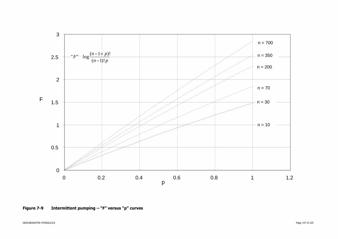
GROUNDWATER HYDRAULICS Page 147 of 225
Figure 7-9 Intermittent pumping – “F” versus “p” curves
0
0.5
1
1.5
2
2.5
3
0 0.2 0.4 0.6 0.8 1 1.2 p
F
n = 700
n = 350
n = 200
n = 70
n = 30
n = 10
pn
pnF
)!1(
)!1(log""

GROUNDWATER HYDRAULICS Page 148 of 225
7.6 EVALUATION OF LONG TERM PUMPING RATE
Frequently the objective of carrying out a pumping test on a bore is to determine its long term
pumping. This needs to be evaluated firstly to see if the bore is capable of supplying the required volume and secondly to ensure that the correct pumping equipment is purchased and installed.
This section gives some indication of how such a rate can be estimated and some of the pitfalls to be avoided when such estimates are made.
Constant Discharge Pumping Test
The constant discharge pumping test with recovery is the most common type of tests used and is suitable for the estimation of long term pumping rates which are of the same magnitude as the test
rate. The method of analysis uses the Modified Non-Steady State flow equations.
The following relates to the practical problems of estimating the long term pumping rate of a
particular bore using data obtained from one or more tests of this type- data being available only from
the pumping bore. The main assumption in the analysis is that the bore will continue to perform, under sustained pumping, in the same manner as indicated during the test.
Procedure
1. The drawdown-time data are plotted on semi-logarithmic graph paper with time on the
logarithmic scale. It is desirable to show the measured discharge rates at the relevant times on this plot.
2. The recovery-time, (or residual drawdown-t/t’), data are plotted on the same sheet to
the same scale.
3. The depth to pump suction is decided upon. Normally the pump suction is placed just
above the seal on the screen assembly.
4. The maximum available drawdown is obtained by subtracting the depth to standing
water level from the depth to pump suction.
5. The working drawdown is obtained by subtracting from the maximum available drawdown an allowance for anticipated drop in standing water level as a result of
seasonal conditions and other reasons.
6. By examination and computation from (i) and (ii) the rate which will give a drawdown
after 100,000 mins (70 days approximately), or any other predetermined period of anticipated demand, which is equal to the working drawdown is called the long term
pumping rate.
At first the method may seem relatively simple but it is beset with certain difficulties and in most cases a certain amount of judgement has to be applied.
Step 6 is of course an important step and some explanation is necessary.
Assume an ideal case where, after an initial curved portion, the drawdown-log time curve becomes a
straight line. If the discharge rate is held constant and there are no hydrologic boundaries, this
straight line should extend to the end of the test. It can be extrapolated also to any time desired, in this case 100,000 minutes has been adopted. In the case of a town water supply, or any other
situation where very long term continuous pumping is required, a period of 1,000,000 minutes i.e. 2 years, would be a better figure. In systems of very high storage/flow ratio a longer period may be
warranted e.g. a bore of relatively low transmissivity being used for a town water supply in the Great
Artesian Basin.
The long term pumping rate is obtained by multiplying the test rate by the ratio of the working
drawdown to the extrapolated drawdown at 100,000 minutes during the test.
510s
sQQ w
TL
.....7.42

GROUNDWATER HYDRAULICS Page 149 of 225
where:
QL = long term pumping rate.
QT = test rate.
sw = working drawdown.
s105 = test drawdown (extrapolated) to 105 minutes, or to the time required.
This rule should be applied with caution particularly in those cases where non-linear head losses are
present. It assumes, if non-linear head loss is present, that it is proportional to the discharge whereas
in fact the non-linear head loss is proportional to the discharge squared. In general it is considered most unwise to predict a long term pumping rate beyond the constant discharge test rate unless you
are very familiar with the conditions in the area and the efficiency of the contractor.
The straight comparison of drawdowns to discharge is most useful when “ironing out” variations in
drawdown caused by relatively small variations in pumping rate during a pumping test.
The figure of 100,000 minutes is more or less an arbitrary end point which seems reasonably convenient to use. The previous period is too short a time and the subsequent log period may be too
long a time for a normal irrigation cycle. A longer period is used of course for Town Water Supply or industrial requirements.
Example
Table 7-7 presents test data obtained by the Queensland Irrigation and Water Supply Commission in
1962.
The bore is located at Biloela in the Callide Valley of Central Queensland.
The semi-logarithmic plot is shown in Figure 7-10 and the analysis is given below.
Table 7-7 Test data from Biloela, Callide Valley
Time
(mins)
Drawdown
(m)
Discharge Rate
(m3/day)
1 2.07 2860
2 2.11
3 2.14
4 2.16
5 2.18 2860
10 2.22
20 2.28
40 2.33
60 2.37 2860
80 2.39
100 2.41
120 2.42
150 2.44 2860
180 2.45 2860
210 2.47
240 2.48 2860
270 2.49
300 2.50
330 2.51 2860
360 2.52

GROUNDWATER HYDRAULICS Page 150 of 225
2.00
2.10
2.20
2.30
2.40
2.50
2.60
1 10 100 1000
Time (mins)
Dra
wdow
n (
m)
Δs = 0.202m
Example
The test data used in this example are from Table 7.7.
Analysis
Long Term Pumping Rate:
Date Tested: August 1962
Top of Packer: 15.5mm BGL
Place Suction 0.15 m above top of packer: 15.35m BGL
Standing Water Level (SWL): 9.95mm BGL
Available Drawdown: 5.40m
Seasonal variation in SWL: 2m
Working Drawdown: 3.40m
At 2860 m3/day, Δs: 0.202m
Drawdown at 1,000 minutes: 2.61m
Drawdown at 100,000 minutes: 2.61 + 2 x Δs
= 3.014 m
Estimated Long Term Pumping Rate:
= (3.40/3.014) x 2860 m3/day
= 3220 m3/day
= 37.2 litres / sec
Transmissivity:
T = 2.3 Q/4πΔs
= 260 m2/day
Figure 7-10 Determination of long term pumping rate

GROUNDWATER HYDRAULICS Page 151 of 225
Variable Discharge Test
If the long term pumping rate for the bore seems to be much greater than the pumping ability of the
test pump then it is desirable to carry out a variable discharge pumping test to enable the non-linear head losses to be determined.
If a variable discharge test, such as a step drawdown test, is carried out then it is possible to determine the equation to drawdown for the bore for a certain period of discharge. Once the equation
to drawdown is determined the long term pumping rate can be calculated.
It is desirable to plot the equation to drawdown, at the time corresponding to the required pumping duration, in the form of drawdown versus discharge on natural scale graph paper. If a non-linear loss
is present this will result in a curved line.
The working drawdown is determined in the same way as described in the previous section.
Working drawdown = Depth to pump suction – Standing water level - seasonal variation.
The working drawdown is then read into the curve of drawdown versus discharge and the rate corresponding to the working drawdown is the long term pumping rate.
The determination of long term pumping rates by using variable discharge tests is desirable, as it accounts for non-linear head loss. This enables the analyst to estimate with some degree of
confidence, long term rates in excess of the test rate.
7.7 SPECIFIC CAPACITY
The Specific Capacity of a discharging bore at a particular time is defined as the ratio of the discharge rate to the drawdown in the bore at that time. It is then the discharge per unit drawdown for a
discharging bore. Its units are m3/day/m.
It is not a fixed value. It varies with both discharge rate and duration of pumping. However, if
calculated at the same time it can give an indication of the changing efficiency of a bore say during
development. Some analysts put a good deal of faith in it. If there is a reasonable degree of confidence in the values of drawdown and discharge being used, then in the absence of more
accurate information, specific capacity can be a useful tool for estimating transmissivity.
Several methods for estimating transmissivity from specific capacity have been published, some of
which are cited below. If we solve equation 10.23 for Q/s (specific capacity), using s as the drawdown in the discharging bore, and rw as the radius of the bore, and assuming that the bore is 100 percent
efficient, we obtain:
SrTt
T
s
Q
ww
2/25.2log3.2
4
.....7.43
which shows the manner in which Q/sw is approximately related to the other constants (T, and S) and
variables (r,t). As rw is constant for a particular bore being pumped, it can be seen that Q/sw is nearly proportional to T at a given value of t, but gradually diminishes as t increases. Thus, for a given bore,
considered 100 percent efficient, and assuming that water is discharged instantaneously from storage
with decline in head, we may symbolise the foregoing statements by the following equation:
where:
.....7.44
B = a constant for the bore, and includes the other terms in equation 7.43.
Driscoll simplifies this further and suggests inserting typical values of T, S, t, and rw into equation 7.43 to obtain an approximate value of transmissivity.
t
B
s
Q
w log

GROUNDWATER HYDRAULICS Page 152 of 225
If typical values are assumed for the variables in the log function of equation 7.43 such that:
t = 1 day;
T = 400 m2/day;
rw = 0.15m;
S = 10-3 for a confined aquifer; and
Sy = 10-1 for an unconfined aquifer;
then the specific capacity at 1 day has the following approximate relationships:
for a confined aquifer:
Q/sw = 0.72 T .....7.45
and for an unconfined aquifer:
Q/sw = 0.98 T .....7.46
It may appear to be presumptuous to use an average transmissivity or even to assume a
transmissivity value at all before one is known. However, because it appears in the log term of equation 7.43, its effect on the value of the divisor in either aquifer case is minimal. For example, if a
transmissivity of 1600 m2/day is used then the value for the confined aquifer would change from 0.72 T to 0.66 T a difference of about 8% for a 300% increase in the value of T.
No bore is 100 percent efficient, but, according to design, construction, age, etc., some bores are more efficient than others.
Thus we see that Q/sw diminishes not only with time but with pumping rate Q. In unconfined aquifers
it may be necessary to take into account delayed yield from storage.
7.8 EVALUATION OF BORE EFFICIENCY
While the radial flow equations provide a very good approximation to actual drawdowns in observation
bores remote from the pumping bore, very seldom if ever, does the actual drawdown in a pumping
bore equal that predicted by the radial flow equations. Invariably the drawdown in the pumping bore is greater, sometimes much greater than that theoretically predicted.
There are many reasons for this increase in drawdown. Some relate to the design of the bore, some to bore construction and others simply to normal groundwater flow which does not always comply
with the assumptions made for the derivation of the equations.
The design factors include:
1. Poor choice of screen apertures, resulting in higher than acceptable flow velocities at
the screen.
2. Less than full screen exposure to the flow resulting in longer flow lines and additional
head loss. This reduced screen exposure could be a consequence of either only part of the aquifer depth being screened (partial penetration) or less than complete screen
exposure around the circumference of the bore.
3. Incorrect filter pack material being used giving rise to greater head loss.
The construction factors would include inadequate development of the bore or screening the wrong
formation.
The hydraulic factors could result from the aquifer parameters being such that the flow near the
screen is no longer linear and additional non-linear head losses come into play.
The ratio of the theoretical drawdown to the actual drawdown is called the bore efficiency.
Regardless of the cause of the difference between the theoretical and actual drawdown in the bore it
is desirable to minimise the difference and make the bore as efficient as possible, and can provide optimal performance.

GROUNDWATER HYDRAULICS Page 153 of 225
Sometimes some of the factors have to be compromised to achieve optimal production from the bore.
For example, it would not be sensible to fully screen a shallow unconfined aquifer and so limit the
depth at which the pump can be set. It would be more prudent in such a case to screen only the bottom one third of the aquifer and allow additional head loss while at the same time achieving a
much greater working drawdown. The pump suction could then be set at two thirds of the aquifer depth. This would then achieve optimal sustained yield while sacrificing efficiency.
If bore efficiency is so important then it is important to have a way to measure it.
The higher the bore efficiency the smaller is the drawdown required in the bore to achieve a certain rate of discharge. This is important for a number of reasons, not the least of which is the energy costs
to pump water.
Jacob was one of the first to try to determine the efficiency of a bore. He assumed that the bore
efficiency was reduced solely by the presence of the non-linear head loss CQ2. He defined the
efficiency of the bore as the ratio of the laminar flow component of the drawdown to the total drawdown. He called the laminar flow term the aquifer loss and the turbulent flow head loss the well
loss.
His was the first step towards determining bore efficiency but it was not correct. While the turbulent
head loss is a contributing factor towards a reduction in bore efficiency it is not the sole contributing factor. Some of the turbulent losses are in the aquifer itself and may not be able to be removed but
more importantly some of the factors contributing to reductions in efficiency are in the laminar flow
component.
7.8.1 When the Equation to Drawdown is Known
A more correct approach is to compare the actual drawdown in the bore with the drawdown would have occurred if the radial flow equations applied right up to the bore. It is also significant that any
such determination will result in changes in bore efficiency with time as well as discharge rate.
The theoretical drawdown at the bore for a 100% efficient bore will be:
Sr
Tt
T
Qs
w
tw 2
25.2log
4
3.2 .....7.47
And the actual drawdown in the pumping bore is:
2
2
25.2log
4
3.2CQ
Sr
Tt
T
Qs
w
aw
i.e. .....7.48
where:
stw = the theoretical drawdown in a 100% efficient bore.
saw = the actual drawdown in the bore.
The bore efficiency is then obtained by comparing equation 7.47 with 7.48.
The efficiency ε of the bore is then:
stw/sa
ε = / .....7.49
To make such a comparison the true values of T, t, S and r should be inserted into equation 7.47. The
actual value of T can be obtained from the pumping tests on the bore and the bore radius is known. The value of S will have to be assumed for confined and unconfined aquifers if it is not known. This
will not present a major error since the range of S would be known and the S value is contained within the log term. The required value of t can also be inserted.
The values of "a", "b" and "C" in equation 7.48 can be obtained from the analysis of step drawdown
tests so sw in equation 7.47 is known for any required value of t.
)25.2
log4
3.2(
2Sr
Tt
T
Q
w
))log(( 2CQQtba
2)log( CQQtbaswa

GROUNDWATER HYDRAULICS Page 154 of 225
Note: remember that the "a" value in equation 7.48 is dependent on the time units used for t in the
equation. It is quite acceptable to use minutes as the time unit in the equation to drawdown if the
equation is to be used on its own. The use of days for the units is dimensionally correct but all that the conversion from minutes to days does is to change the value of the "a" term by a constant
"b x log 1440". However, if we are comparing equations as we must do in determining the bore efficiency then the units must be consistent. The "t" in equation 7.48 must be in days and the
"a" term must be consistent. If the "a" term had been calculated on the basis of a 1 minute intercept
and "t" had been expressed in minutes in equation 7.48 then to convert "t" to day units simply add "b x log 1440" i.e. 3.16 x b to the "a" term.
If we divide both sides of equations 7.47 and 7.48 by Q then the efficiency of the bore at one unit of time can be expressed as:
ε = ( ) / ( ) .....7.50
If the time at which the efficiency is being determined is1 then (b log t) in equation 7.48 becomes 0.
The transmissivity of the aquifer is constant and 2.3/(4πT) in equation 7.47 is equal to "b" which has
been determined from the pumping tests.
For convenience, in the absence of more reliable information, S could be taken as 10-3 for a confined
aquifer and 10-1 for an unconfined aquifer.
Example
Calculate the efficiency of the Richmond Town Bore No. 3 for discharge rates 1000 m3/day and
3000 m3/day at times 1 minute, 1 day and 1 week after pumping discharge commenced.
The equation to drawdown for the bore has been determined previously as:
swt = (a + b log t) Q + C Q2
= (3.1 x 10⁻³ + 5.34 x 10⁻⁴ log t) Q + 8.1 x 10⁻⁷ Q2
Since the time units in this equation are minutes they will have to be changed to days so that the
equation can be compared with equation 7.43. The "a" term has to be changed by adding "b x log 1440". The "a" term now becomes 4.78 x 10⁻³. All other terms remain the same.
The equation then becomes:
swt = (4.78 x 10⁻³ + 5.34 x 10⁻⁴ log t) Q + 8.1 x 10⁻⁷ Q2
where "t" is now in days.
The radius of the bore is 0.075m.
It is in a confined aquifer so we can take S as 10-3 and T (2.3/(4πb) is 345 m2/day.
Case 1 (at time 1 minute)
For Q = 3000 m3/day
Sr
Ttb
w
2
25.2log
= 0.000534 x log {(2.25 x 345) / (1440 x 0.0752 x 0.001)}
= 0.00266
a + CQ = 4.78 x 10⁻³ + 8.1 x 10-7 x 3000
= 0.00553
ε = 0.00266 / 0.00553
= 48%
The same procedure can be used to determine the efficiencies at the other times and rates to give the
results tabulated in Table 7-8.
Sr
Tt
T w
2
25.2log
4
3.2 CQtba log

GROUNDWATER HYDRAULICS Page 155 of 225
Table 7-8 Bore efficiencies for Richmond Town bore no. 3
Time
(mins)
(Days) Discharge Rate
(m3/day)
Bore Efficiency (η)
(%)
1 0.000694 1000 67.70
1 0.000694 3000 47.85
1440 1 1000 77.25
1440 1 3000 59.89
10080 7 1000 78.90
10080 7 3000 62.22
From Table 7-8 it can be seen that in this case the efficiency decreases with an increase in discharge
rate but increases with the duration of pumping. If continuous pumping is not required then in some instances it may be more economical to pump at lower rates for longer periods.
7.8.2 When the Equation to Drawdown is Not Known
The above procedure is able to be used if the equation to drawdown for the bore is known. In many instances the equation is not known and only a single pumping test is available. In such cases the
following procedure can be used.
The efficiency is determined using the same comparison as in the previous section i.e. the drawdown
in the bore operating at 100% efficiency is compared with the actual drawdowns in the pumping bore.
The theoretical drawdown at the bore for a 100% efficient bore will be:
Sr
Tt
T
Qs
w
tw 2
25.2log
4
3.2
and the actual drawdown in the pumping bore is taken from a plot of the test results. This analysis is
exactly the same as the previous case but it is limited to the test discharge rate. It does not give the
ability to determine the efficiency for rates other than the test rate.
Once again T can be calculated from the test data, rw is known and S can be assumed for confined
and unconfined conditions.
Driscoll uses more approximations still. Using the approximations to specific capacities given in
equation 7.45 and equation 7.46 for confined and unconfined aquifer conditions respectively, he compares the specific capacity of a theoretical bore of 100% efficiency with the specific capacity
(Q/sw) of the pumping bore at time 1 day.
This is a very quick method and gives a good indication of the efficiency of the bore.
By way of comparison, the values of corrected drawdowns for Richmond Town Bore No. 3 as plotted
in Figure 7-3 were extrapolated to 1 day. The specific capacities were calculated for each of the steps and the bore efficiencies estimated using Driscoll's approximation. The bore efficiencies for each
of the steps were also calculated using equation 7.50. Table 7-9 gives the efficiencies calculated
using each method.
Table 7-9 Comparison of efficiency calculations
Time
(day)
Discharge Rate
(m3/day)
Efficiency (%)
Using
Equation 7-50
Using
Approximate Method
1 1135 76 72
1 1640 71 67
1 2180 66 61
1 2725 62 57
1 3270 58 54

GROUNDWATER HYDRAULICS Page 156 of 225
SECTION 8: EVALUATION OF AQUIFER PROPERTIES WITHOUT PUMPING TESTS
8.1 INTRODUCTION
The most accurate method of determining aquifer parameters is to carry out a properly conducted pumping test on a bore with measurements of drawdown and discharge rate at selected times after
pumping commenced. However, in many instances data from pumping tests are not available and aquifer parameters have to be estimated. The methods outlined below provide some means of
obtaining reasonably reliable results.
8.2 AREAL METHODS
8.2.1 Numerical Analysis
The partial differential equation for two dimensional non-steady state flow can be expressed as:
t
h
T
S
y
h
x
h2
2
2
2
.....8.1
where:
h = the head at any point whose coordinates are x,y.
If we let the infinitesimal lengths x and y be expanded so that each may be equivalent to a finite
length "a" and similarly let t be considered equivalent to Δt. A plan representation of the region of
flow to be studied may then be subdivided by two systems of equally spaced parallel lines at right angles to each other. One system is oriented in the x direction, the other in the y direction, and the
spacing of lines equals the distance "a". A set of 5 gridline intersections, or nodes (observation bores), as shown in Figure 8-1, is called an array.
Figure 8-1 Numerical analysis array
The first two differentials in equation 8.1 can be expressed in terms of the head values at the nodes
(bores) in the array as:
2
031
2
2 2
a
hhh
x
h .....8.2
and
2
042
2
2 2
a
hhh
y
h .....8.3
where the subscripts refer to the numbered nodes in Figure 8-1.
4
0 1
2
x
y
3
a

GROUNDWATER HYDRAULICS Page 157 of 225
Substituting these closely equivalent expressions in equation 8.1, and letting t
h be considered
equivalent to Δh0/Δt, we obtain:
t
h
T
Sahhhhh 0
2
04321 4 .....8.4
where:
Δh0 is the change in head at node (bore) 0 during the time interval Δt.
This is merely an introduction to numerical analysis.
Example
This data was presented originally in imperial units but has been converted for these notes.
Stallman tried this method successfully on several such arrays in the Arkansas Valley, Colorado, during
the winter of 1965-66. Bores 1- 4 were spaced 304m apart, so that "a" (304/√2) was equal to 216m.
From the estimated values of T and S, "a" normally is determined from the convenient empirical relation a2S/T =10± days but in the Arkansas Valley, nearby boundaries made it necessary to use
a2S/T = 4± days. The elevations of the measuring points at each of the five wells were determined above a convenient arbitrary datum, and the water levels, measured in metres above datum, were
obtained from automatic water level sensors. The winter data from the Nevius site near Lamar, Colorado were plotted as shown in Figure 8-2, in which Ρh, in mm, represents the left hand side of
equation 8.4, and Δh0/Δt is in mm/day.
From equation 8.4 note that the slope of the straight line, which Stallman drew form a least-squares fit, is Ρh/( Δh0/Δt) = 3.99 days.
Hence:
a2S/T = 3.99 days
The value T/S is known as the Hydraulic Diffusivity.
S was known from neutron moisture probe tests, made during periods of both high and low water levels, to be about 0.18.
a2 = 4.7 x 10⁴ m2
then:
T = (a2S/ Ρh)/ (Δh0/Δt)
= (4.7 x 104 x 0.18) 3.99
= 2.12 x10³ m2 / day
This value of T was in close agreement with the results of a nearby pumping test.
Conversely, if the value of T were known, the storage coefficient could have been determined.

GROUNDWATER HYDRAULICS Page 158 of 225
Figure 8-2 Numerical analysis example
8.2.2 Flow-Net Analysis
In analysing problems of groundwater flow, a graphical representation of the flow pattern can be of
considerable assistance and may provide solutions to problems not readily amenable to mathematical solution. This is a logical, and on occasions eye-opening, follow-on from the normal water level or
potentiometric level contours which are frequently drawn during groundwater investigations. They can be used to determine aquifer characteristics of transmissivity and storage coefficient, or, knowing
these, the volume extracted. Recharge areas can be detected also by this means.
The first significant development in graphical analysis of flow patterns was made by Forchheimer (1930), but additional information was given by Casagrande (1937, p. 136, 137) and Taylor (1948).

GROUNDWATER HYDRAULICS Page 159 of 225
Legend:
___20___ depth below sea level in metres
flow line
Figure 8-3 Typical flow net
A "flow net", which is a graphical solution of a flow pattern, is composed of two families of lines or
curves (see Figure 8-3). One family of curves, termed equipotential lines (solid lines on map),
represent contours of equal head in the aquifer, and may be contours of the potentiometric surface or of the water table. Intersecting the equipotential lines at right angles (in isotropic aquifers) is another
family of curves (dashed lines on map) representing the streamlines, or flow lines, where each curve indicates the path followed by a particle of water as it moves through the aquifer in the direction of
decreasing potentiometric head.
Although the real flow pattern contains an infinite number of flow and equipotential lines, it may be
represented conveniently by constructing a net that uses only a few such lines, the spacing being
conveniently determined by the contour interval of the equipotential lines. The contour interval indicates that the total drop in head in the system is evenly divided between adjacent pairs of
equipotential lines; similarly the flow lines are selected so that the total flow is equally divided between adjacent pairs of flow lines. The movement of each particle of water between adjacent
equipotential lines will be along flow paths involving the least work, hence it follows that, in isotropic
aquifers, such flow paths will be normal to the equipotential lines, and the paths are drawn orthogonal to the latter.
The net is constructed so that the two sets of lines form a system of "squares". Note on the map that some of the lines are curvilinear, but that the "squares" are constructed so that the sum of the lengths
of each line in one system is closely equal to the sum of the lengths in the other system.
Let Figure 8-4 represent one idealised "square" of Figure 8-3, whose dimensions are Δw and Δl.

GROUNDWATER HYDRAULICS Page 160 of 225
Figure 8-4 Elemental square
Then, by rewriting Darcy's Law as a finite-difference equation for the flow, ΔQ, through this elemental
"square" of thickness b, we obtain:
ΔQ = -K b Δw (Δh/Δl) .....8.5
Since, by construction, Δw = Δl, then:
ΔQ = -TΔh .....8.6
If:
nf = number of flow channels;
nd = number of potential drops; and
Q = total flow
then:
Q = nf ΔQ or ΔQ = Q/nf .....8.7
and
h = nd Δh or Δh = h/nd .....8.8
Substituting equations 8.7 and 8.8 in equation 8.6 we obtain:
Q = -T (nf/nd)h .....8.9
or
hnn
QT
df )/( .....8.10
Conversely Q can be determined if T is known.
Example
Figure 8-3 presents the flow net for a hypothetical situation in which it is known that the discharge
from sub-area A is 100 000m3/day. It shows 15 flow channels surrounding the sub-area, hence nf = 15. The number of equipotential drops between the 30- and 60- m contours is 3, so nd = 3. The
total potential drop between the 30 and 60 m contours is 30 m, so h = 30 m.
Then, from equation 8.10:
)30)(3/15(
000,100T
= 667 m2/day
The value of T thus determined is for a much larger sample of the aquifer than that determined by a pumping test on a single bore. This method has been largely neglected, but is deserving of more
widespread application.
h1
h2
Δl
Δw

GROUNDWATER HYDRAULICS Page 161 of 225
8.3 ESTIMATING TRANSMISSIVITY
8.3.1 General
In some ground-water investigations, such as those of a reconnaissance type, it may be necessary to estimate the transmissivity of an aquifer from the specific capacity (yield per unit of drawdown) of
bores, as the determination of T by use of some of the equations discussed above may not be feasible. On the other hand, some of our modern quantitative studies, such as those for which
electric-analog models or mathematical models are constructed, require a sufficiently large number of
values of T so that transmissivity-contour maps (T maps) may be constructed.
In unconfined aquifers, such T maps generally require also the construction of water table contour
maps and bedrock-contour map, from which may be obtained maps showing lines of equal saturated thickness, b, for we have seen that T = Kb. For example, a quantitative investigation of a
240 kilometre reach of the Arkansas River Valley, in eastern Colorado, required a T map based upon
about 750 values, or about 0.65 values per square kilometre. About 25 of these values were obtained from pumping tests, selected as reliable tests from a greater number of tests conducted. About
200 values of T were estimated from the specific capacity of bores, by one of the methods to be described. About 525 values were estimated by geologists from studies of logs of bores and test
holes, by methods to be described. Thus, only about 3 percent of the values were actually determined from pumping tests.
8.3.2 Specific Capacity of Bores
The Specific Capacity of a discharging bore at a particular time is defined as the ratio of the discharge rate to the drawdown in the bore at that time. It is then the discharge per unit drawdown for a
discharging bore. Its units are m3/day/m.
It is not a fixed value. It varies with both discharge rate and duration of pumping. However, if
calculated at the same time it can give an indication of the changing efficiency of a bore say during
development.
Some analysts put a good deal of faith in it. If there is a reasonable degree of confidence in the values
of drawdown and discharge being used, then in the absence of more accurate information, specific capacity can be a useful tool for estimating transmissivity.
Several methods for estimating transmissivity from specific capacity have been published, some of which are cited below. If we solve equation 6.23 for Q/s (specific capacity), using s as the drawdown
in the discharging bore, and rw as the radius of the bore, and assuming that the bore is 100 percent
efficient, we obtain:
SrTt
T
s
Q
ww
2/25.2log3.2
4 .....8.11
which shows the manner in which Q/sw is approximately related to the other constants (T,S) and variables (r,t). As rw is constant for a particular bore being pumped, we see that Q/sw is nearly
proportional to T at a given value of t, but gradually diminishes as t increases by the amount log t. Thus, for a given bore, considered 100 percent efficient, and assuming that water is discharged
instantaneously from storage with decline in head, we may symbolise the foregoing statements by the
following equation:
t
B
s
Q
w log .....8.12
where:
B = a constant for the bore, and includes the other terms in equation 8.11.
Driscoll simplifies this further and suggests inserting typical values of T, S, t, and rw into equation 8.11 and obtaining an approximate value of transmissivity.

GROUNDWATER HYDRAULICS Page 162 of 225
If typical values are assumed for the variables in the log function of equation 8.11 such that:
t = 1 day;
T = 400 m2/day;
rw = 0.15m;
S = 10-3 for a confined aquifer; and
Sy = 10-1 for an unconfined aquifer;
then the specific capacity at 1 day has the following approximate relationships:
for a confined aquifer:
Q/sw = 0.72 T .....8.13
and for an unconfined aquifer:
Q/sw = 0.975 T .....8.14
It may appear to be presumptuous to use an average transmissivity or even to assume a
transmissivity value at all before one is known. However, because it appears in the log term of equation 8.11, its effect on the value of the divisor in either aquifer case is minimal. For example, if a
transmissivity of 1600 m2/day then the value for the confined aquifer would change from 0.72 T to 0.66 T a difference of about 8%.
No bore is 100 percent efficient, but, according to construction age, etc., some bores are more efficient than others. Jacob (1947, p. 1048) has approximated the head loss resulting from the
relatively high velocity of water entering a bore or bore screen as being proportional to some higher
power of the velocity approaching the square of the velocity, which in turn is nearly proportional to Q2; thus:
head loss = CQ2
where:
C = a constant of proportionality.
Adding this to equation 8.12:
)1(log
2
ww s
CQ
t
B
s
Q .....8.15
Thus we see that Q/sw diminishes not only with time but with pumping rate Q. In unconfined aquifers
it may be necessary to adjust factor B to further account for delayed yield from storage.
The relation of specific capacity to discharge and time for a particular bore in a confined aquifer is
shown in Figure 8-5 (Jacob, 1947, Figure 5; converted to metric for these notes).

GROUNDWATER HYDRAULICS Page 163 of 225
Figure 8-5 Typical specific capacity - time - discharge curves
In an uncased bore in, say, sandstone, rw may be assumed equal to the radius of the bore, but in
screened bores in unconsolidated material, in which the finer particles have been removed near the screen by bore development, or in gravel-packed bores, the effective rw generally is larger than the
screen diameter. Jacob (1947) described a method for determining the effective rw and the well loss
(CQ2) from a step drawdown test, and other methods are given earlier in this chapter.
Most other investigators have neglected well loss in their equations, which are equations for bores of
assumed 100 percent efficiency, such as equation 8.12, but some have adjusted for this loss by selection of an arbitrary constant for bores of similar construction in a particular area or aquifer, which
generally gives satisfactory results when used with caution.
Theis (1963a, p. 331-336) gave equations and a chart, based upon the Theis equation, for estimating T from specific capacity for constant S and variable t, with allowance for variable bore diameter but
not bore efficiency. Brown (1963, p. 336-338) showed how Theis' results may be adapted to artesian aquifers. Meyer (1963, p. 338-340) gave a chart for estimating T from the specific capacity at the end
of one day of pumping, for different values of S and for bore diameters of 0.5 (0.15), 1.0 (0.30) and
2.0 (0.61) ft (m). Bedinger and Emmett (1963, p. C188-C190) gave equations and a chart for estimating T from specific capacity, based upon a combination of the Thiem and Theis equations, and
upon average values of T and S for a specific area, for bore diameters of 0.5 (0.15), 1.0 (0.3) and 2.0 (0.61) ft. (m). Hurr (1966) gave equations and charts based upon the Theis and Boulton (1954a)
equations, which allow for delayed yield from storage, for determining T from specific capacity at different values of t for a bore 1.0 ft (0.3 m) in diameter. None of the methods just cited includes
corrections for bore efficiency, but this can be added in an approximate manner.
8.3.3 Rough Method
Using the Steady State Flow Equation, Equation 6.5:
1
2
21
log)(2
3.2
r
r
ss
QT .....8.16
Let:
r1 = the effective radius of the bore, in this case 0.3 m;
r2 = radius of influence of bore, assume 300 m;
s1 = drawdown in the bore (one only drawdown, no test has been carried out); and
s2 = 0.

GROUNDWATER HYDRAULICS Page 164 of 225
then:
1000log2
3.2
1s
QT
1
(2
3*3.2
s
Q)
If r2 were taken as 3000 m, then log r2/r1 would only be increased to 4. This is a 25% alteration but the order of T has not changed. Apart from the assumed values of r the solution must be approximate
as the bore has been assumed to be 100% efficient.
8.3.4 Logs of Bores
As noted in Section 8.3.1, about 525 values of t out of 750 total values, in the Arkansas Valley of
Eastern Colorado, were estimated by geologists from studies of logs of bores, and from drill cuttings from test holes. Wherever possible pumping tests were carried out on bores for which, or near which,
logs were available; otherwise, test holes were drilled near the bore tested. From several of many such pumping accompanied by logs, the values of T were carefully compared against the
water-bearing bed or beds, and, as T = Kb, the total T was distributed by cut and try among the
several beds, according to the following equation:
nnm
n
m bKbKbKbKbKT ......332211
1
.....8.17
From this the following table was prepared, comparing average values of K for different alluvial materials in the valley.
The same geologist who prepared Table 8-1 then carefully examined the logs of other bores and test holes, for which no pumping tests were available. He assigned values of K to each bed of known
thickness, on the basis of the descriptive words used by the person who prepared the log. The values of K assigned may have been equal to, or more or less than values given in the table (depending upon
cleanliness, sorting, mixing, etc), and thus necessarily involved subjective judgement; however, as
experience is gained, the geologist can estimate K and T with fair to good accuracy. The T values from all sources also are compared carefully with the saturated-thickness map.
This method for estimating T has been used successfully in the Arkansas Valley in Colorado, in the Arkansas Valley in Arkansas and Oklahoma (Bedinger and Emmett, 1963), in Nebraska, in California,
and can be used elsewhere.
8.3.5 Laboratory Analysis
Laboratory determinations for K of cores of consolidated rocks, such as partly to well cemented
sandstone, may be used in place of estimates. Reconstitution of disturbed samples of unconsolidated material is not possible, however, so laboratory determinations for K generally do not give reliable
values. However, they may be very useful in indicating relative values. Table 1-2 at the end of Section 1 gives indicative values of hydraulic conductivity for various rock types.
The above methods may also be used by the geologist in measuring exposed sections of rocks
containing water-bearing beds.

GROUNDWATER HYDRAULICS Page 165 of 225
Table 8-1 Average values of hydraulic conductivity of alluvial material in the Arkansas
Valley, Colorado
Material Hydraulic Conductivity
(m/day)
Gravel, coarse 305
Gravel, medium 286
Gravel, fine 265
Sand, very coarse to gravel 246
Sand, very coarse 204
Sand, coarse to very coarse 143
Sand, coarse 73
Sand, medium to coarse 33
Sand, medium 16.5
Sand, fine to medium 8.2
Sand, fine 4.1
Sand, very fine to fine 1.7
Sand, very fine 0.8
Clay 0.4
(Courtesy R. T. Hurr)
8.4 ESTIMATING STORAGE COEFFICIENT AND SPECIFIC YIELD
8.4.1 Confined Aquifers
In measuring sections of exposed rock which dip down beneath confining beds to become confined
aquifers, or in examining logs of bores or test holes in confined aquifers, S can be determined fairly closely from Table 8-2. The table is merely the calculation of the first term of equation 3.6 for
compression of water alone:
i.e.
Table 8-2 Storage coefficient approximation
b
(m)
S S/b
(m-1)
1 5 x 10⁻⁶ 5 x 10⁻⁶
10 5 x 10⁻⁵ 5 x 10⁻⁶
100 5 x 10⁻⁴ 5 x 10⁻⁶
1000 5 x 10⁻³ 5 x 10⁻⁶
One may either multiply the thickness in metres by 5 x 10⁻⁶ or interpolate between values in the first
two columns, thus for b = 300m, S = 1.5 x 10⁻³, etc. Values thus obtained are not absolutely correct; they represent the minimum value of S as no adjustments have been made for porosity or for
compressibility of the aquifer. However, the values so obtained are reliable estimates.
8.4.2 Unconfined Aquifers
It is more difficult to estimate the specific yield of unconfined aquifers than the storage coefficient of confined aquifers, but it can be done. It should be remembered that the specific yield applies only to
the material in the zone of water-table fluctuation and to the material within the cones of depression
of pumping bores. In general the specific yield ranges between 0.1 and 0.3 (10-30 percent), and long periods of pumping may be required to drain water-bearing material.
))1(
(sw EE
gbS

GROUNDWATER HYDRAULICS Page 166 of 225
Thus, in the absence of any determinations whatever, as in a rapid reconnaissance study, we would
not be far off by assuming that, for supposed long periods of pumping, the specific yield of an
unconfined aquifer is about 0.2. If logs of bores or tests holes are available, careful study of the grain sizes present, degree of sorting, and cleanliness, might allow a better estimate of S, which might then
be more or less than 0.2. A few laboratory determinations of the specific yield of disturbed samples may refine the estimate and allow extrapolation to similar material in the logs of other wells or test
holes, but such determinations are more likely to be too large than too small. The values of specific
yield obtained from reliable long pumping tests would greatly refine the estimates, and could be extrapolated to similar types of material elsewhere in the same aquifer. The values obtained from
neutron-moisture probes (Meyer, 1962) could be similarly extrapolated.
8.4.3 Water Balance
In any aquifer system a water balance must exist. This balance is expressed very simply by the
following equation:
Recharge+Groundwater Inflow = Draft+Groundwater Outflow +/- Change in Storage ...8.18
The Recharge includes such items as natural recharge from rainfall, or streamflow, artificial recharge and excess irrigation.
The Draft includes evapotranspiration, withdrawals for irrigation, industrial, Town Water Supplies, stock and domestic uses.
The change in storage is expressed as ASΔh where:
A = surface area of the water table.
S = storage coefficient or specific yield.
Δh = change in water level during the period of analysis.
This is probably the most accurate means of determining a regional storage coefficient.
8.4.4 Barometric Efficiency
The storage coefficient of a confined aquifer may be approximated by utilising the barometric efficiency (BE) of the aquifer.
A reduction in barometric pressure results in a rise in ground-water levels. The ratio of the change in groundwater pressure to the change in atmospheric pressure is called the barometric efficiency.
The barometric efficiency is defined as:
BE = ξgΔh/Δpa .....8.19
where:
ξ = density of water.
g = gravitational acceleration.
Δh = change in potentiometric level due to Δpa.
Δpa = change in atmospheric pressure.
The barometric efficiency can be interpreted as a measure of the competence of the overlying
confining beds to resist pressure changes; thick impermeable confining strata are associated with high barometric efficiencies, whereas thinly confined aquifers will display low values.
The barometric efficiency of unconfined aquifers is zero, i.e. a change in atmospheric pressure does not result in a change in water level.
It can be shown that the barometric efficiency is related to the storage coefficient of an aquifer by the
following equation:
BEE
gbS
w
.....8.20

GROUNDWATER HYDRAULICS Page 167 of 225
where:
S = storage coefficient.
ζ = porosity.
ξ = density of water.
g = gravitational acceleration.
b = thickness of the aquifer.
Ew = bulk modulus of elasticity of water.
BE = barometric efficiency.
Thus, from the barometric efficiency of a confined aquifer, an estimate of its storage coefficient can
be obtained.
8.4.5 Tidal Efficiency
Just as atmospheric pressure changes produce variations of potentiometric levels, so do tidal
fluctuations; both earth tides and ocean tides. The ocean tides vary the load on confined aquifers extending under the ocean floor. The earth tides result from varying gravitational forces on the
aquifer from both the moon and the sun. These forces can cause expansion and contraction of the aquifer which result changes in porosity and accompanying changes in groundwater levels.
Unlike the atmospheric pressure effect, tidal fluctuations are direct; i.e. as the sea level increases, so too does the ground water level. The ratio of potentiometric level amplitude to tidal amplitude is
known as the tidal efficiency of the aquifer.
Jacob showed that tidal efficiency (TE) is related to barometric efficiency BE by:
TE = 1 – BE .....8.21
Thus, tidal efficiency is a measure of the incompetence of overlying confining beds to resist pressure changes.
The storage coefficient of an aquifer can be computed from observations of the tidal efficiency by
replacing BE by 1 - TE in equation 8.20.
It has been further shown that the amplitude h of groundwater fluctuation at a distance x from the
shore is given by:
TtSx
x ehh 0/
0 .....8.22
where:
hx = the amplitude of groundwater fluctuations at distance x from shore.
h0 = the amplitude of tidal fluctuations at the shore.
x = distance of the observation bore from the shore.
t0 = the tidal period.
T = the transmissivity.
It has been further shown that the time lag tL of a given maximum or minimum water level in a bore after high or low tide occurs can be obtained from:
)4/( 0 TStxtL .....8.23
If the storage coefficient has been estimated from the tidal efficiency then a value of transmissivity
could also be estimated from equation 8.21.

GROUNDWATER HYDRAULICS Page 168 of 225
SECTION 9: CORRECTIONS AND EFFECTS TO BE ALLOWED FOR WHEN ANALYSING
9.1 GENERAL
Many of the assumptions which have been made in developing the equations presented previously are not met in nature and corrections have to be made to the data before they can be applied.
Some of the effects which have to be taken into account are:
delayed yield in unconfined aquifers;
increased drawdown caused by dewatering in unconfined aquifers;
anomalies in drawdown readings;
partial penetration;
antecedent pumping conditions;
possible development during pumping;
proximity of recharging or discharging boundaries;
water temperature variations in hot bores;
anisotropy, non-homogeneity and finite bore diameter;
variations in barometric pressure; and
tidal effects.
9.2 DELAYED YIELD FROM STORAGE
This effect is taken into account quite adequately by Boulton's analysis for unconfined aquifers exhibiting delayed yield. However if other equations are to be used then the value of storage
coefficient which has been calculated may have to be calculated many times throughout the test until the stable storage coefficient, or in this case specific yield, has been determined.
9.3 INCREASED DRAWDOWN CAUSED BY DEWATERING
Jacob suggested a correction to allow for dewatering which was presented in Section 9.4.3. The
correction applies to drawdowns measured in observation bores during a pumping test. These drawdowns should be small in relation to the saturated thickness of the aquifer.
Jacob's correction to drawdown is:
s' = s - s2/2b
where:
s' = the corrected drawdown.
s = the observed drawdown.
b = the aquifer thickness.
The corrected value is then used instead of the measured drawdown in the flow equations for
confined aquifers.
A correction should also be applied to the storage coefficient which is obtained when using these
equations. The correction to storage coefficient which has been applied after the correction to
drawdown is as follows:
S = (b-s)/b x S'

GROUNDWATER HYDRAULICS Page 169 of 225
where:
S = the corrected value of Storage Coefficient.
b = aquifer thickness.
s = observed drawdown.
S1 = apparent storage coefficient calculated using corrected drawdowns and transmissivity.
In many cases when pumping a bore the aquifer adjacent to the bore is dewatered causing a
reduction in saturated thickness of the aquifer and hence a reduction in the apparent transmissivity at
that point.
If the Modified Non-Steady State Flow Equations are used to analyse such a test the plot results in a
curve which increases in slope as time progresses. This increase in slope is caused by a continuing reduction in aquifer thickness. A correction should be made to allow for its reduction if transmissivity
is to be calculated from information from the discharging bore alone. The correction presented by
Jacob (Section 9.2) would be a good first approximation. The corrected drawdowns should not be used when determining long term pumping rates.
9.4 ANOMALIES IN DRAWDOWN READINGS
The data being analysed in any pumping test are subject to human error. Anomalies being encountered in the data should be carefully weighed before attributing them to a boundary condition.
If they are not consistent with other readings it is possible that they should be discarded. However,
they should not be discarded too quickly or before an investigation is carried out as to why the anomaly has occurred.
9.5 PARTIAL PENETRATION
A bore whose length of water entry is less than the aquifer thickness which it penetrates is known as
a partially penetrating bore. For such a bore the flow pattern differs from that for a fully penetrating bore with the same discharge because the average length of flow line is longer and so a greater
resistance to flow occurs.
For practical purposes, this results in the following relationships between two similar bores, one
partially and one fully penetrating the same aquifer.
If Qp = Q, then, swp > sw,
and
if swp = sw, then, Qp < Q
where:
Q = bore discharge for the fully penetrating bore.
sw = drawdown in a fully penetrating bore.
swp = drawdown in a partially penetrating bore.
Qp = discharge from a partially penetrating bore.
The alteration to the flow lines and so the magnitude of the drawdown applies not only to the bore
but to conditions in the aquifer at a considerable distance from the bore, which will give erroneous values of storage coefficient in observation bores installed in this effected zone.
The drawdowns in observation bores inserted into the top and the bottom of the aquifer respectively
and at the same distance from the discharging bore will be different if they are affected by partial penetration.
It has been found, however, that the effect of partial penetration is negligible beyond a distance of twice the saturated thickness from the bore. For this reason, observation bores which are to be used
in the calculation of storage coefficient should not be located closer to the partially penetrating pumping bore than twice the saturated thickness of the aquifer.

GROUNDWATER HYDRAULICS Page 170 of 225
The equations for determining the hydraulic characteristics of an aquifer are based upon the
assumption that the discharging bore taps the full thickness; observed water level drawdowns in bores
tapping less than the full thickness should be corrected before they are used in the equations. Equations and values are given by Jacob.
Such corrections generally are unnecessary if the observation bores are placed in pairs, one of each pair tapping the top part of the aquifer just below the cone of depression, and the other tapping the
bottom part of the aquifer. The drawdowns in each bore of each pair (corrected by subtracting s2/2b if
necessary) are plotted, then averaged graphically, not arithmetically (in a semi-logarithmic plot the arithmetic and graphical average is the same but this is not so in a logarithmic plot). It has been
found that for relatively thin unconfined aquifers, it is convenient to place three pairs of observation bores at distances from the discharging bore of b, 2b, 4b.
It is necessary to adjust for partial penetration effects if type curve solutions on log-log paper or
"distance-drawdown" curves on semi-logarithmic paper are to be used. In the case of "time-drawdown" curves on semi-logarithmic paper the correction is necessary for the calculation of S
but, for a sufficiently long pumping period it may not be necessary in computing T.
9.6 ANTECEDENT CONDITIONS
The standing water level in a bore may vary prior to the commencement of a test. Such variations
may be caused by tides, barometric pressure changes or other conditions. It is desirable to monitor
the water level in the bore for a period prior to the commencement of the test and extend the variation trend through the test. If possible pre-test observations are compared with records of
barometric pressure and, if applicable, tidal variations.
Correction of the data from a static or recovery test is generally necessary and occasions arise where
other pumping test data has to be corrected for antecedent pumping conditions. The only time that
the uncorrected data can be used is when the test follows a condition of a steady flow. The meaning of steady flow in this context is a flow condition which could not be expected to change by a
measurable amount over a period equal to that covered by the test in question, if the test had not been carried out. This period includes the no flow condition.
Depending on the particular bore this would generally require that the flow of the bore had not been altered in any way for at least 24 hours prior to the new test. If there is any doubt as to whether any
residual effect remains from earlier alteration in discharge, this can be checked quickly by evaluating
the maximum correction, which will be required at the end of the test, to see if this is significant.
Corrections for variation in discharge are computed by use of the equation:
δs = ΔQb log10 t1/t2
where:
δs = change in head caused by an increase (or decrease) in discharge of ΔQ between t1 and
t2 after this increase (or decrease) commenced to operate.
b = constant (Δs/Q), a function of the transmissivity of the bore.
ΔQ = change in discharge rate.
An increase, or positive value of delta Q, produces an increase in head loss or a reduction in pressure
while a decrease or negative value of delta Q produces a decrease in head loss or an increase in
pressure. The effects of all previous increases or decreases in discharge can be added or subtracted to give the net effect at any given point of time.
To compute this net correction it is obviously necessary to know the value of b. However, an approximate value only is necessary and this can be obtained from the early portion of the test being
analysed, before the effect of antecedent variations become apparent. If the value of b from the corrected data differs significantly from that used as a first approximation in computing the correction,
this new value of b may be substituted in the correction equation as a second approximation. This is
rarely necessary as quite a large change in b does not make a very large change in the correction.
If the test results are analysed using the Eden-Hazel method as presented in Section 7, the
corrections for antecedent conditions are carried out automatically.

GROUNDWATER HYDRAULICS Page 171 of 225
9.7 POSSIBLE DEVELOPMENT DURING PUMPING
Pumping is a form of mechanical development and it is possible that during a pumping test the bore is
still developing. Smaller drawdowns will be recorded in the pumping bore during the latter stages of such a test than would be expected if the aquifer conditions immediately adjacent to the bore had
remained constant throughout the test.
It is possible also that a collapse in the aquifer may have occurred during the pumping test and this
would result in a much larger drawdown during the final stages of the test than that which would be
expected. If this is the case then this final condition would control the future performance of the bore, unless the bore was brought back to the original condition. It would not be valid to discard this as
being a rogue value and determine the equation to drawdown for the bore from all previous drawdowns.
Negative values of C, the non-linear head constant, would indicate development during the test.
On occasions, development during testing, or collapses in the aquifer during testing, have been attributed to other causes.
9.8 PROXIMITY OF BOUNDARIES
So far, the aquifers we have considered in flow equations have all been assumed to be of infinite areal extent. Some aquifers are sufficiently large to satisfy this assumption reasonably well, at least during,
say, the period of a pumping test. Many aquifers have hydrologic boundaries, such as a nearby stream
or lake, and (or) geologic boundaries, such as the relatively impermeable bedrock wall of an alluvium-filled valley, or a fault. Such boundaries, if close enough to a discharging bore, may
invalidate the results obtained by use of the flow equations, unless suitable adjustments are made.
9.8.1 Method of Images
The method of images used for the solution of boundary problems in the theory of heat conduction in
solids has been adapted to the solution of boundary problems in groundwater flow. In this method, imaginary bores or streams, referred to as images, are arbitrarily placed at proper locations to
duplicate hydraulically the effect on groundwater flow caused by the real hydrologic or geologic boundary.
Following heat-flow terminology, a discharging image bore is regarded as a point sink, a recharging image bore as a point source; a discharging image stream (drain) is regarded as a line sink, a
recharging image stream as a line source. By use of various combinations of such sinks and sources,
corrections for almost every conceivable type and shape of boundary have been made so as to permit solution of the appropriate groundwater flow equation. We will take up a few of these; for others see
Ferris (1959), Ferris and others (1962), Walton (1962), and Kruseman and De Ridder (1970).
9.8.1.1 Recharging Boundary
If a bore in an unconfined aquifer near a large perennial stream hydraulically connected to the aquifer
is pumped, obviously the cone of depression cannot extend beyond the stream as the water level in such a stream remains relatively constant. Such a situation is shown in Figure 9-1A and
Figure 9-1B (Ferris and others, 1962).
In Figure 9-1A the nearly straight partly penetrating perennial stream is assumed to be straight and
fully penetrating and, hence, equivalent to a line source at constant head. The hydraulic counterpart
in an infinite aquifer is shown in Figure 9-1B, where a recharging image bore, or point source, has been placed on a line connecting the real and image bores, at right angles to the stream, at the same
distance, a, from the stream. The recharge and discharge rates, Q, are assumed equal. The resulting cone of depression (heavy solid line) is the algebraic sum of the cone of depression of the real bore
(dashed line) and the cone of impression of the recharging image bore (dashed line) and the former intersects the level of the stream as it should. The flow net for these conditions is shown in
Figure 9-2 - note that if the image bore and its flow net are removed, the flow net on the left is that
of the real bore obtaining water by induced infiltration from the streams.
In most field situations streams only partly penetrate the aquifer and the cone of depression may
extend beneath and beyond the stream bed. Hence when analysing pumping test data, when the distance to the recharge boundary is determined, this distance may be only the effective distance to a
fully penetrating stream which has the same hydraulic effect as the real stream.

GROUNDWATER HYDRAULICS Page 172 of 225
One of the first applications of the image-bore theory to groundwater flow was made by Theis (1941),
who developed an equation and presented a graph for computing the percentage of the water
pumped from a bore near a stream that 1s diverted from the stream at a known distance from the well (see also Theis, 1963b, p. C101-C105, Theis and Conover, 1963, p. C106-C109).
In 1938 Theis (Wenzel and Sand, 1942, p. 45) developed a formula for determining the decline in artesian head at any distance from a drain (line sink) discharging water at a constant rate.
Figure 9-1 Idealised section views of a discharging well in a semi-infinite aquifer bounded by a perennial stream, and of the equivalent hydraulic system in
an infinite aquifer
Ferris (1950) developed the same formula and gave data for plotting a type curve of his drain
function, C(u) versus u2.
Stallman (Ferris and others, 1962, p. 126-131) developed equations and a type curve for determining the decline in artesian head at any distance from a linear stream or drain of constant water level
(head).
Jacob (1943) developed methods based upon an unconfined aquifer subject to a constant rate of
recharge (W) and bounded by two parallel fully penetrating streams. From the shape of the water
table, as determined from water-level measurements in bores, may be estimated the base flow (groundwater runoff) of the streams or the average rate of groundwater recharge.

GROUNDWATER HYDRAULICS Page 173 of 225
Figure 9-2 Generalised flow net showing stream lines and potential lines in the vicinity of a discharging well dependent upon induced infiltration from a nearby
stream
Rorabaugh (1964) gave methods, equations, and charts for estimating the aquifer constant T/S from natural fluctuations of water levels in observation bores in finite aquifers having parallel boundaries.
Examples of such aquifers are: a long island or peninsula, an aquifer bounded by parallel streams, and an aquifer bounded by a stream and a valley wall. For similar finite aquifers, Rorabaugh (1964) also
developed methods for estimating groundwater outflow (as into streams) and for forecasting
streamflow recession curves. The component of outflow related to bank storage 1s computed from river fluctuations; the component related to recharge from irrigation and precipitation is computed
from water levels in a bore. Rorabaugh's methods should have widespread application 1n areas having the required boundary conditions.
9.8.1.2 "Impermeable" Barrier
Figure 9-3A below (Ferris and others, 1962, fig. 37) shows a discharging well 1n an aquifer bounded on the right by a barrier of relatively impermeable material. Hence it is assumed that no groundwater
can flow across the barrier. The image system in the hydraulic counterpart which permits a solution of the real problem by use of the flow equations, is shown in Figure 9-3B. Here an image bore with
discharge equal to that of the real bore is situated the same distance (a) from the barrier. The dashed theoretical cones of depression of the real and image bores intersect to form a groundwater divide at
the barrier, across which no flow can take place, thus satisfying the conditions. The real resultant
cone of depression (heavy line) is the algebraic sum of the dashed theoretical cones of depression. Figure 9-4 depicts the flow nets of the two-bore system. If the image bore and flow net are
removed, the flow net on the left is the one that would be observed for a discharging bore near the "impermeable" boundary.
In the case of two parallel impermeable boundaries (a channel aquifer) the effects of image bores will
be cumulative and the number of image bores required is never ending. This results in a progressive steepening of the semi-logarithmic plot. Particular reference to a bore with two parallel boundaries
can be found in U.S.G.S. Water Supply Paper I536-E p.p. 156, 157, and in Kruseman and De Ridder, 1970.

GROUNDWATER HYDRAULICS Page 174 of 225
9.8.1.3 Drawdown Interference From Discharging Bores
Regardless of the extent of an aquifer, other discharging bores within the area of influence (circular
area of cone of depression at radius where drawdown in an observation bore would be negligible at time t, say, <0.01 m), or within overlapping area of influence, constitute boundaries of the point-sink
type. Likewise, a recharging bore would be a boundary of the point-source type.
If T and S are known, as from discharging bore tests, then the effect of one discharging bore upon a
non-discharging bore is readily obtained by use of equation 6.18, equation 6.19 solved for
u = r2S/4Tt, and a table of W(u) v (u), for any distance r for known or assumed values of t and Q, or for any time t and for known or assumed values of r and Q. In this manner, families of
semi-logarithmic curves showing drawdowns at various distances from the discharging bore for various discharge rates can be drawn.
Figure 9-3 Idealised section views of a discharging bore in a semi-infinite aquifer
bounded by an impermeable formation, and of the equivalent hydraulic
system in an infinite aquifer
In preparing families of curves of this type, note that once the curves become straight lines, only a
few points are required to define the straight parts. Theis (1963c, p. C10-C15) has prepared a simple chart for the computation of drawdowns in the vicinity of a discharging bore.
Where many discharging bores are mutually interfering with each other, the problem becomes much
more complex and is best handled by an electric analog model or digital computer. If the aquifers are artesian, and have low values of T and S, the interference effects spread far 1n relatively short
periods and increase relatively rapidly with time at a given distance.

GROUNDWATER HYDRAULICS Page 175 of 225
Figure 9-4 Generalised flow net showing stream lines and potential lines in the vicinity
of a discharging well near an impermeable boundary
9.8.1.4 Application of Image-Bore Theory
Now that we have discussed several types of hydrogeologic boundaries and their simulation by the method of images, what do we do with them, and how do they affect the results of pumping tests?
From the preceding discussions, it should be evident that for a discharging bore in an aquifer bounded
by a relatively impermeable barrier, as in Fig. 9.4 a time versus drawdown plot for an observation bore near the pumped bore will be steepened (greater drawdown) at the value of t after the cone of
depression reaches the barrier. Conversely, if the discharging bore were near a perennial stream, as in Fig. 9.2, the curve for an observation bore near the pumped bore would be flattened (less drawdown)
at the value of t after the stream is reached. Computation of T and S by the Theis or similar equations
would then be valid only for the early data before the boundary effects changed the slope of the curve. This would offer no problem for a confined aquifer; but, in an unconfined aquifer, sufficient
time might not have elapsed to allow for reasonably complete drainage from storage, as discussed earlier.
Ferris and others (1962, p. 161, 162) described a method of plotting s versus t or r2/t for matching with the Theis type curve that permits of a solution for T and S and also for the distance from the
observation bore to the image bore. If the boundary is concealed, as a hidden fault, three or more
observation bores are required to locate the boundary (see Ferris and others, 1962, p. 164-166; Moulder, 1963).
Rather than describe the somewhat laborious method referred to in the first part of the preceding paragraph, we will take up a much simpler method devised by Stallman (1963b), for the solution of
single-boundary problems involving either a source or a sink. From Figure 9-2 and Figure 9-4,it is
evident that if s0 is the drawdown is an observation bore, and sp and si are the components of that drawdown caused, respectively, by the pumped bore and by the discharging or recharging image
bore, then s0 is the algebraic sum of sp and si , or:
s0 = sp +/- si .....9.9

GROUNDWATER HYDRAULICS Page 176 of 225
For this condition, equations 10.18 and 10.19 may be rewritten, respectively:
))((4
))()((4
0 uWT
QuWuW
T
Qs ip .....9.10
and
up = rp2S/4Tt, and ui = ri
2 S/4Tt .....9.11
where rp is the distance from the pumped bore to the observation bore, and ri is the distance from the observation bore to the image bore.
In equation 9.11, up and ui are seen to be related thus:
ui = (ri/rp)2up, or ui = K12up .....9.12
where:
K1 = ri/rp .....9.13
Note: the K1 in equations 9.12 and 9.13 of Stallman is simply a constant of proportionality and is not
to be confused with the K used for the hydrologic conductivity.
Stallman plotted a family of logarithmic type curves of W(u) versus 1/u for many values of his
K1 = r1/rp as shown in Figure 9-5.
In this analysis the drawdown in the observation bore, s0, is plotted against time since pumping
started, t, on logarithmic graph paper. For an aquifer in which a single boundary is suspected, the
plotted curve is superimposed on the family of type curves in Figure 9-5, and a match point found for values of ΡW(u) and i/up, and corresponding values of s0 and t respectively, in the same way as
matching the Theis type curve. Equation 9.10 can then be used to solve for T, after which equation 9.11 can be used to solve for S. (Note: By writing equations 9.10 and 9.11 for a particular
curve that is followed by the observed data, the value of ri can be calculated from equation 9.13).
If the suspected boundary is absent, and hence the aquifer is extensive, the observed data should follow the heavy parent type curve which is the Theis type curve. If a boundary exists, the observed
data will follow the parent curve until the boundary is first "felt", then it will deviate from the parent curve along one of the modified curves. Deviations below the parent curve are caused by recharging
images; those above by discharging images.

GROUNDWATER HYDRAULICS Page 177 of 225
Figure 9-5 Family of type curves for the solution of the modified Theis formula

GROUNDWATER HYDRAULICS Page 178 of 225
9.9 WATER TEMPERATURE VARIATIONS IN HOT BORES
By virtue of the aquifer depth the water in many flowing artesian bores is extremely hot. One bore at
Birdsville in southwest Queensland is some 1,220 metres in depth and has a temperature of 99°c at the surface. The back pressure at the surface on this bore is some 1210 kPa with zero flow.
It will be appreciated that the density of the water at this very high temperature is much lower than what it would be at a lower temperature. With this lower density the head of water to maintain the
pressure in the aquifer will be much higher.
If the flow from such a bore is stopped for any significant period then heat will be lost from the water to the surrounding ground, and the water cools. The most significant drop in temperature of course is
near the surface of the bore with a less significant drop as the aquifer is approached.
With the lowering in temperature the density of the water increases and the apparent pressure at the
surface decreases.
If a static test (recovery test) is carried out on such a bore then the pressure rises during the early stages of the test but the rate of rise does not conform with the theoretical rate as the water begins
to cool. In fact in some cases the pressure may begin to drop. The analyst must be aware of such conditions and how to overcome them.
Unfortunately there is no hard and fast rule for correcting for this condition as yet but a rough approximation based solely on densities indicates that the difference in head for the Birdsville bore at
99°C and 37.8°C is some 30 metres. This assumed a linear variation in temperature from the surface
to the aquifer which is unlikely to be correct.
9.10 VARIATIONS IN ATMOSPHERIC PRESSURE
A change in atmospheric pressure results in a change in the force applied to both the aquifer matrix
and the water within the aquifer.
The effect of this change in applied force is zero in an unconfined aquifer and there is no change in water level. However, in a confined aquifer, while the competence of the overlying confining material
is able to absorb the increase in load, such changes can and do have a significant impact on groundwater levels. The way in which the water level responds to changes in atmospheric pressure is
directly related to the storage coefficient of the aquifer. The relationship between water level change and change barometric pressure is called the barometric efficiency and will be discussed in more detail
in Section 8. The barometric efficiency can be used to determine storage coefficient.
Suffice to say at this stage that a drop in atmospheric pressure results in a rise in groundwater level in a confined aquifer. In the Great Artesian Basin, some bores which have recently stopped flowing will
start to flow again if a low pressure event such as a cyclone passes over the area. Of course such a recommencement of flow will be temporary.
9.11 TIDAL EFFECTS
Tidal effects can influence water levels in confined aquifers. The effect of tides is the opposite from
that of changes in atmospheric pressure. Rising pressure caused by higher tides result in rises in groundwater levels.
There are two types of tidal effects which need to be taken into account; ocean tides and earth tides.
Both of these effects are sinusoidal in nature.
The rising and falling sea levels impose varying loads on the confining layer of the aquifer where it
extends out under the sea. The change in groundwater level is greatest near the coast and attenuates as the distance from the coast increases.
Earth tides are a result of the gravitational attraction, predominantly between the moon and the earth. These gravitational forces act on the matrix of the aquifer alternately stretching it and compressing it.
These changes in structure cause changes in groundwater levels.

GROUNDWATER HYDRAULICS Page 179 of 225
9.12 OTHER FACTORS TO BE CONSIDERED
Other factors such as anisotropy, non-homogeneity and finite diameter of the facility should also be
taken into account but will not be discussed here. Methods of allowing for anisotropy and finite diameter of the bore can be found in the references.

GROUNDWATER HYDRAULICS Page 180 of 225
SECTION 10: APPLICATION OF AQUIFER PROPERTIES
10.1 INTRODUCTION
Knowledge of aquifer properties is a necessary pre-requisite for the solution of most groundwater problems. A few of the everyday problems are presented in this section together with an indication of
how aquifer parameters are used to solve them.
10.2 VOLUME IN STORAGE
The total volume of water which is stored in a saturated material is given by:
VT = V'Sζ .....10.1
where:
VT = total volume of water stored.
V'T = total saturated volume.
ζ = porosity.
However, not all of this water is available for extraction. Some water is held by the soil matrix under
gravity drainage, and additional water is unavailable as it is needed to provide the necessary gradient for groundwater flow. When considering the extractable volume of any groundwater basin some lower
limit, or dead storage level, should be determined and only water stored above that level considered in the calculations.
On this basis the total extractable volume stored in a ground-water basin is given by:
VE = VS x SY .....10.2
where:
VE = total extractable volume.
VS = saturated volume above dead storage level.
SY = specific yield of the material.
The volume of saturated material can best be obtained by obtaining average saturated thicknesses throughout the area, normally by an examination of private facilities or investigation facilities, and
multiplying this average figure by the total area being investigated. Shape factors of the basin may have to be taken into account.
Storage coefficient is not used to determine the total volume stored in an aquifer.
10.3 VOLUME REMOVED FROM STORAGE
In a case of a confined aquifer the net volume of water which has been removed from the aquifer may be obtained by multiplying the storage coefficient by the change in potentiometric head during
that period. The total volume which has been removed, of course, will have to take into account any recharge effects which occurred during the period. If the water level fell below the top of the confined
aquifer then the specific yield would have to be used for that period.
In the case of an unconfined, semi-unconfined, or semi-confined aquifer a drop in water level would normally be associated with drainage of some of the saturated material. In this case the net volume
removed during a certain period is obtained by multiplying the specific yield of the dewatered material by the change in potentiometric head during that period.
Volume removed from storage = S Δh .....10.3
where:
S = storage coefficient for a confined aquifer.
S = specific yield of dewatered material for any other type of aquifer.
Δh = change in head during the period considered.

GROUNDWATER HYDRAULICS Page 181 of 225
If the volumes removed for irrigation, stock, industrial and own water supplies are negligible or are
known from metering, then the volume removed by evapotranspiration can be computed.
It must be remembered that this is a net volume removed. To get the total volume removed any recharge events and down valley groundwater flow will have to be taken into account.
10.4 GROUNDWATER FLOW
The groundwater flow in any section of aquifer can is obtained by using the transmissivity, the
hydraulic gradient, and the area through which the water is moving.
In the case of leaky aquifers the main transmission system is the aquifer proper even though the
semi-pervious material which overlies the aquifer acts as a storage. The transmissivity which is obtained from pumping tests is invariably the transmissivity of the aquifer proper.
The groundwater flow through an aquifer is obtained from:
Q = TiW .....10.4
where:
Q = total groundwater flow through the section considered.
T = the average transmissivity in that section.
i = the hydraulic gradient (i.e. the slope of the potentiometric surface).
W = width of the section being considered.
The value of transmissivity varies with the saturated thickness in the alluvium and for this reason the
transmissivity values may not be constant across a particular cross-action. In cases such as this the cross-section is divided into smaller sections and groundwater flow computed for each of these
smaller sections. The total groundwater flow in the cross-section is then the sum of the flows in each of the smaller sections.
A special case of groundwater flow is the determination of flow into excavations which is important for
the mining industry and for construction operation which involves excavation below the water table. This situation is covered briefly in section 10.7.
Total flow in an aquifer can also be obtained by utilising flow nets.
10.5 LEAKAGE
From the analysis of tests carried out on leaky aquifers the leakage coefficient, (1/c), can be
determined.
From this, the rate of leakage from an overlying aquifer to a lower aquifer can be computed by using Darcy's Law.
Darcy's Law may be written as:
Q = -KiA
where:
K = the hydraulic conductivity.
i = the hydraulic gradient.
A = area through which the flow is occurring.
For vertical flow in the semi-confining layer or leaking layer Darcy's Law can be written as:
Ab
sKQ
|
| .....10.5

GROUNDWATER HYDRAULICS Page 182 of 225
where:
K|= vertical hydraulic conductivity of the semi-pervious layer.
B|= saturated thickness of the leaking layer.
S = drawdown in the main aquifer.
A = area through which leakage is occurring.
The leakage coefficient (K'/b1) is then the rate of flow from the leaking zone to the aquifer per unit
drawdown per unit area.
If the average leakage coefficient is obtained for an area then for each drawdown in the main aquifer the volume of water which will migrate to the lower aquifer per unit time per unit area can be
computed. Summing this over the total area the total volume which has migrated to the aquifer is able to be computed.
This is important if an unconfined aquifer overlies a leaky aquifer and is separated by a leaky material.
The major recharge to the system could occur in the unconfined zone and migrate to the lower aquifer through this leaking zone.
By analysing the demands which are placed on the upper unconfined aquifer the area to be covered by a well field tapping the lower aquifer and still maintaining equilibrium with the natural recharge
conditions can be determined.
10.6 DRAWDOWN INTERFERENCE EFFECTS
10.6.1 Drawdown Within the Area of Influence
Regardless of the extent of an aquifer, other discharging bores within the area of influence or within
overlapping areas of influence, constitute boundaries, of the point-sink type. Likewise, a recharging bore would be a boundary of the point-source type. If T and S are known, from discharging bore
tests, then the effect of one discharging bore upon a non-discharging bore is readily obtained by use
of equation 6.18 and equation 6.19 (solved for u = r2S/4Tt, and then calculate W(u) as the first two terms of the series i.e. W(u) = -0.577216 -logeu) or equation 6.24 and for any distance "r"< for
known or assumed values of t and Q, or for any time "t" for known or assumed values of r and Q.
Example
A bore, in an aquifer with transmissivity of 400 m2/day and a storage coefficient of 10-3, is pumped at 1000 m3/day. What is the drawdown in a bore 200m from the pumping bore after 1 day?
From equation 6.19:
u = r2S/4Tt
= 0.025
W(u) = (-0.577216 -logeu)
= 3.112
From equation 6.18:
)(4
uWT
Qs
= 0.619m
Or using equation 6.24:
Sr
Tt
T
Qs
210
25.2log
4
3.2
= 0.619m
The drawdown at any point in an aquifer system is a summation of the drawdown effects from all
discharging bores within that system.

GROUNDWATER HYDRAULICS Page 183 of 225
10.6.2 Comparative Spread of Area of Influence
Lohman (1965, p. 109, 110) showed that:
)3.2/4
2
10
25.2QTS
Ttr
)/(10
25.2ssS
Tt .....10.6
For a given set of conditions, all terms except r and S may be considered constant; then, using C as a
constant of proportionality:
r2 = C/S
If we multiply both sides by π then:
πr2 = A = C'/S .....10.7
Equation 10.7 may be used to compare the area of influence in a confined aquifer, A1 having a storage
coefficient of, say, 5 x 1O-5 with the area of influence in an unconfined aquifer, A2 having a specific yield of, say, 0.20. Assuming that T, Q, and s are the same for both aquifers, and that t also is the
same and long enough that u ≤ 0.05 & that the cone of depression in the unconfined aquifer has had
time to be drained, then:
345
2
1 10*45
10*2
2.0/'
10*5/'
C
C
A
A
Thus under the assumed conditions, the area of influence in the confined aquifer is 4,000 times larger
than that in the unconfined aquifer, or, the ratio of the radius extending to the circumference of negligible drawdown in the confined aquifer, to that in the unconfined aquifer, is:
3
2
2
2
1 10*4r
r
whence:
2.6310*4 3
2
1
r
r
Thus, changes in artesian head or pressure in a confined aquifer spread outward very readily from the
discharging bore, although it requires time for the drawdown to be measurable at a given distance from a discharging bore. By contrast, in an unconfined aquifer, changes in water level occur very
slowly as gravity drainage takes place, so the cone of depression enlarges very slowly.
10.6.3 Determination of Radius of Influence
If it is assumed that we are dealing with an aquifer in porous media and that the assumptions for the
modified non-steady state equations apply then the drawdown at any point within the area of influence at a given time t is given by:
Sr
Tt
T
Qs
2
25.2log
4
3.2
The radius of influence at any time t is the radius at which the drawdown is zero.
For this to apply the log term must be zero i.e. the value within the log term must equal 1.
Thus at the radius of influence:
S
Ttr 5.10 .....10.8

GROUNDWATER HYDRAULICS Page 184 of 225
where:
r0 = radius of influence at time t after pumping commenced.
T = transmissivity.
T = time since pumping commenced.
S = storage coefficient or specific yield, depending on the aquifer type.
From the above it can be seen that the radius depends only on time transmissivity and storage
coefficient and is completely independent of discharge rate. The discharge rate determines the
magnitude of the drawdown within the cone of depression but not the areal extent.
This is a very simple means of determining the radius of influence and, if used with care and common
sense, can be used to provide a reasonable approximation even for those aquifers which are not in porous media.
10.7 DRAINAGE PROBLEMS
Water tables near ground surface can be controlled by construction of drains or bores to maintain
level at or below specified depths.
Drains are designed in several ways. Some are composed of coarse sand or gravel so that their
permeability is higher than the surrounding porous media. Water flows readily through them and they serve as outlets for draining surrounding groundwater. Horizontal lines of open jointed tile or
perforated pipe are widely employed for drains. Other drains are simply open ditches which intercept
ground-water whenever the water table rises above the bottom of the ditch.
Drains have many applications, only a few of which can be mentioned here. An earth dam usually
contains drains near its toe to prevent saturation of the downstream face. Most foundations of structures contain drains around their perimeters to reduce hydrostatic pressure or water entrance.
Modern highways often contain sub-drains to avoid saturation of highway grade. On agricultural lands,
adequate drainage systems are essential for stabilising water tables below the root zone. High water tables may result naturally in flat lands bordering rivers, lakes, or the ocean, or may be produced
artificially by percolation from excess irrigation water.
To regulate water levels within narrow limits over a large area, drains are made in parallel lines at
depths and spacing governed by local crop and soil or aquifer conditions.
The design and construction of drains for controlling ground-later levels will not be covered in this
text. Basic principles involved, however, are the same as those described in preceding pages.
Pumping bores also may control water levels, the process being identical to bores providing water supplies. Where drainage bores are employed on agricultural lands, the extracted water may be
reapplied to the land for irrigation or may be wasted depending on the salinity of the water. A battery of spears, i.e., a line of small diameter bores, is often installed for dewatering construction sites. Relief
bores are placed near the toes of dams and levees to lower water tables and thereby reduce uplift
pressures produced by seepage under the structure.
10.7.1 Mine Dewatering
Mine dewatering is a special case of drainage and is not covered fully in these notes. However, there are applications of hydraulic parameters which can be of assistance in many cases and some of these
are given below.
There are two main types of mining operations namely:
open cut mining; and
underground mining.
In the case of open cut mining all aquifers overlying the material being mined are intersected and
inflows from all aquifers have to be taken into account in dewatering calculations.

GROUNDWATER HYDRAULICS Page 185 of 225
However, in many underground mining operations it is not necessary to remove all water overlying
the zone being mined. For instance a coal seam may need to be dewatered to enable safe and
economic working conditions. The coal seam may be overlain by other shallower aquifers which are not hydraulically connected to the coal seam itself. It is not necessary to dewater these overlying
aquifers as long as a connection does not exist.
The removal of water from the seam itself involves two separate processes:
depressurising the seam by removing water from elastic storage; and
dewatering the seam by draining water from the pores of the matrix.
The first process involves the use of the storage coefficient and the second involves the use of the
specific yield.
If there is no hydraulic connection between the seam being mined and the overlying aquifers then
both of these processes can be carried out without affecting the water levels in the overlying aquifers.
In isotropic aquifers it is possible to calculate discharge and drawdown for individual bores, multiple
bores (borefields), open pits and strip mines using simple analytical methods. Some of these methods
are presented below.
10.7.1.1 Single Bore Dewatering System
On some occasions it is possible to dewater a working area by pumping from a single bore. If the bore is deep enough, the pumping rate is high enough and the transmissivity and storage coefficient are
suitable then the cone of depression may be such that the water level will be drawn down below the bottom of the working area. A pumping test should be carried out on the bore to determine the
aquifer parameters and assess its long term pumping capacity. Since dewatering is normally a long
term process it is reasonable to assume that steady state conditions can be approximated. However, it would be prudent to find out at what time after pumping began that steady state conditions would be
approached. This can be done by either by plotting the time-drawdown on natural scale and selecting a time when the rate of drawdown increase appears to be very small or by plotting time-drawdown on
a semi-logarithmic scale and choosing a time from that. Under equilibrium conditions the rate at which
a bore will have to pump to produce a certain drawdown is given by equations 10.9 to 10.11 for unconfined and confined aquifers respectively:
unconfined aquifer:
.....10.9
confined aquifer:
....10.10
....10.11
....10.12
where:
Q = discharge rate (m3/day).
K = hydraulic Conductivity (m/day).
H = potentiometric head in bore before pumping (m).
hw = potentiometric head in bore during pumping (m).
h = potentiometric head at distance r from the bore (m).
r0 = radius of cone of depression (radius of influence) (m).
rw = effective radius of bore (m).
r = radial distance from bore (m).
w
w
rR
hHKQ
/log3.2
)(22
)/log3.2
( 2
K
rRQHh
wrr
hHKbQ
/log3.2
)(2
0
Kb
rrQs
2
/log3.2 0

GROUNDWATER HYDRAULICS Page 186 of 225
s = drawdown at distance r from the bore (m).
10.7.1.2 Equivalent Bores
Equations 10.9 to 10.12 for individual bores can on occasions be applied to circular and some rectangular arrays of bores around a similar shaped area to be dewatered. On such occasions, the
arrays of bores can be replaced by one bore (or equivalent circular pit) with a radius equivalent to the effective radius of the array and having an equivalent drawdown effect similar to the array of bores.
This equivalent radius is then used in the equations 10.9 to 10.12. The effective radius re is the radius
of a circle having the same area as the base of the rectangle.
If the rectangular array is such that the base length of the pit (y) is ≤ 1.5 times the base width (x) the
pit can be regarded as an equivalent bore with an equivalent bore radius of re= √(xy/π).
For cases where (y) > 1.5 (x) the flow can be treated as parallel flow through 2 sides and 2 ends plus
radial flow at each corner. This case is considered in Strip Pits below.
10.7.1.3 Multiple Bores - Bore Fields
In most cases a single bore will not be sufficient to provide adequate dewatering and a number of
bores will be required around the working area. The cones of depression from each of the bores will intersect and the drawdown at any point within the area of influence will be the sum of the individual
drawdowns from each bore.
The first step in this process is to identify a number of control points within the working area and the
drawdown necessary at each of those points to dewater the working area.
Next the number, location and pumping rates for each of the dewatering bores have to be determined. The locations of the bores may be influenced by physical features such as roads or
buildings. It is prudent to construct one bore and carry out a pumping test to calculate the transmissivity and storage coefficient for the area as well as a range of possible pumping rates for the
bore before attempting to determine the number and locations of the remaining bores.
Once these parameters have been obtained the locations of the bores can be set and drawdowns calculated at each of the control points. Once again equations 10.9 to 10.12 can be used to calculate
rates and drawdowns. A spreadsheet can be used to prepare a table such as Table 10-1. The spreadsheet enables various combinations of the number of bores, bore locations and individual
pumping rates to be trialled before the final bore installation begins. Using different combinations, the drawdowns at each of the control points are determined and checked against the design
requirements.
Example of borefield design
To enable safe excavation at the site below the groundwater levels at points A, B, C and D need to be
drawn down 15m below the present standing water level when excavation begins in 4 months time. This will be achieved by pumping from bores 1, 2, 3 and 4. At what rates do the bores have to be
pumped to achieve the required water levels?
The transmissivity of the aquifer being dewatered is 100 m2/day and the storage coefficient is 0.01.
Bore1 Bore 2
Bore 3 Bore 4
A B
C
D

GROUNDWATER HYDRAULICS Page 187 of 225
The drawdown “sw” at distance “r” from a pumping bore at time “t” after pumping commenced at
discharge rate “Q” is given by:
The drawdown at any point in the aquifer is the summation of the individual drawdowns resulting
from each pumping bore.
The pumping bores must of course be drilled deep enough to enable such drawdowns to occur.
Table 10-1 is a spreadsheet showing the design of the borefield.
Table 10-1 Drawdowns at control points during dewatering
Pumping
Bore
Pumping
Rate
(m3/day)
Control Point A Control Point B Control Point C Control Point D
Distance From
Pumping
Bore (m)
Drawdown (m)
Distance From Pumpin
g Bore (m)
Drawdown (m)
Distance From
Pumping Bore
(m)
Drawdown (m)
Distance From
Pumping Bore
(m)
Drawdown (m)
1 1300 35 5.58 122 2.99 134 2.80 87 3.69
2 1600 146 3.23 55 5.71 77 4.86 108 4.00
3 1200 59 4.15 117 2.84 105 3.05 63 4.03
4 1100 130 2.42 63 3.69 34 4.77 80 3.27
Total Drawdown
15.38 15.23 15.48 14.99
Design Drawdown
15.00 15.00 15.00 15.00
Occasionally it is necessary to dewater a working area while still maintaining the groundwater levels
on one or more zones outside of the working area. One way of achieving this is to pump water from
the dewatering bores and then recharge the water back into the aquifer where required. This technique is illustrated in Figure 10-1.
Figure 10-1 Recharging pumped water to maintain water levels in sensitive areas
10.7.1.4 Strip Pits
In strip pits (such as open cut mines) which intersect aquifers, water flows into the pit as parallel flow
through each of the four sides and as radial flow through the corners as shown in Figure 10-2. This model is equivalent to the discharge from one bore, with a quarter of the bore at each corner of the
pit, and parallel flow through two sides and two ends. Equations 10.13 and 10.14 give the relevant equations for this model for the unconfined and confined aquifer situations.
)25.2
(log4
3.2210Sr
Tt
s
Qsw

GROUNDWATER HYDRAULICS Page 188 of 225
Figure 10-3 illustrates flow into a strip pit which intersects more than one aquifer. It highlights the
fact that, regardless of depth of the pit, the maximum drawdown that can occur in any aquifer is to
the bottom of that aquifer. In the multi aquifer case each aquifer must be treated separately.
At any specified time t the lateral extent of the parallel flow can be considered to be equal to the
radius of influence of the bore quadrant located at each corner. Using the Modified Non-Steady State flow equations, the radius of influence is defined as that distance where the drawdown is zero.
The radius of influence is determined by equation 10.9 as r = 1.5 √Tt/S.
Parallel Flow to Sides and Ends
Quadrant of Circle
Radial Flow
Total Flow to Strip Pit:
= Flow through 2 sides
+ Flow through 2 ends
+Flow through 4 quadrants
Strip Pit
Figure 10-2 Groundwater flow into a strip pit
Ground Surface
SWL SWL
Aquifer 1
Aquifer 2
Min
e D
isc
ha
rge
Note: (1) The maximum drawdown in any aquifer is the distance from SWL to the bottom of that aquifer. The drawdown in aquifer 2 will then be greater than that in aquifer 1.
(2) The radius of influence in any aquifer at any time is independent of discharge rate. It depends
only on T and S for that aquifer. The magnitude of drawdown within the cone of depression is dependent on the discharge rate.
Figure 10-3 Multiple aquifer flow into a strip pit

GROUNDWATER HYDRAULICS Page 189 of 225
Knowing the radius of influence at time t and knowing the drawdown in aquifer at the pit face at the
same time it is possible to determine the drawdown at any distance r from the pit at that time. This
can be done using the equations or simply by using semi logarithmic paper and plotting drawdown against logarithm of distance. A straight line joining drawdown in the pit (plotted as 1 metre from the
side of the pit) and zero drawdown at the radius of influence. It is important to remember that the water level in an aquifer cannot be drawn down below the base of the aquifer. Hence, in the case of
multiple aquifers the maximum drawdown in each aquifer is determined by the base of the aquifer
and not necessarily to the water level in the pit itself.
Equations 10.13 and 10.14 can be used to calculate the flow into the pit:
unconfined aquifer:
....10.13
confined aquifer:
....10.14
where:
Q = discharge rate (m3/day).
K = hydraulic Conductivity (m/day).
H = potentiometric head in pit before pumping (m).
hw = potentiometric head in pit during pumping (m).
h = potentiometric head at distance r from the pit (m).
r0 = radius of cone of depression (radius of influence) (m).
rw = effective radius of bore (say 1m) at corner quadrant (m).
r = radial distance from pit (m).
L0 = maximum length of drawdown influence from side of pit (use r0) (m).
s = drawdown at distance r from the pit (m).
x = width of base of pit (m).
y = length of base of pit (m).
If the pit is of constant depth during its life then the drawdown in the pit will remain constant and the inflow rate will decline in the same manner as for a constant drawdown pumping test. However, in
mining practice, while the pit depth does remain relatively constant for long periods, the pit area
continues to expand. This expansion continues to intercept more and more aquifer and new drawdown conditions have to be taken into account. This can be done in discrete time steps and does
not have to be a precise and continuous operation.
0
22
0
22
2
)()(2
)/log(3.2
)(
L
hHKyx
rr
hHKQ
w
00
)()(2
)/log(3.2
)(2
L
hHKbyx
rr
hHKQ
w

GROUNDWATER HYDRAULICS Page 190 of 225
SECTION 11: GROUNDWATER MANAGEMENT
11.1 GROUNDWATER YIELD ANALYSIS
11.1.1 Bore Yields
Quite frequently the objective of carrying out a pumping test on a particular bore is to determine a
long term pumping rate at which the bore can be equipped for irrigation, town water supply or some other purpose.
The following paragraphs give some indication of how such a rate can be estimated and some of the pitfalls to be avoided when such estimates are made.
11.1.1.1 Constant Discharge Pumping Test
The constant discharge pumping test with recovery is suitable for the estimation of long term pumping rates which of the same magnitude of the test rate. The method of analysis uses the
Modified Non-Steady State flow equations.
The following relates to the practical problems of estimating the long term pumping rate of a
particular bore using data obtained from one or more tests of this type- data being available only from the pumping bore. The main assumption in the analysis is that the bore will continue to perform,
under sustained pumping, in the same manner as indicated during the test.
Procedure
1. The drawdown-time data are plotted on semi-logarithmic graph paper with time on the
logarithmic scale. It is desirable to show the measured discharge rates at the relevant times on this plot.
2. The recovery-time, (or residual drawdown-t/t’), data are plotted on the same sheet to
the same scale.
3. The depth to pump suction is decided upon. Normally the pump suction is placed just
above the seal on the screen assembly.
4. The maximum available drawdown is obtained by subtracting the depth to standing
water level from the depth to pump suction.
5. The working drawdown is obtained by subtracting from the maximum available
drawdown an allowance for anticipated drop in standing water level as a result of
seasonal conditions and other reasons.
6. By examination and computation from (i) and (ii) the rate which will give a drawdown
after 100,000 mins (70 days approximately), or any other predetermined period of anticipated demand, which is equal to the working drawdown is called the long term
pumping rate.
At first the method may seem relatively simple but it is beset with certain difficulties and in most cases a certain amount of judgement has to be applied.
Step 6 is of course an important step and some explanation is necessary.
Assume an ideal case where, after an initial curved portion, the drawdown-log time curve becomes a
straight line. If the discharge rate is held constant and there are no hydrologic boundaries, this
straight line should extend to the end of the test. It can be extrapolated also to any time desired, in this case 100,000 minutes has been adopted. In the case of a town water supply, or any other
situation where very long term continuous pumping is required, a period of 1,000,000 minutes i.e. 2 years, would be a better figure. In systems of very high storage/flow ratio a longer period may be
warranted e.g. a bore of relatively low transmissivity being used for a town water supply in the Great Artesian Basin.
The long term pumping rate is obtained by multiplying the test rate by the ratio of the working
drawdown to the extrapolated drawdown at 100,000 minutes during the test.

GROUNDWATER HYDRAULICS Page 191 of 225
510s
sQQ w
TL .....11.1
where:
QL = long term pumping rate.
QT = test rate.
sw = working drawdown.
s105 = test drawdown (extrapolated) to 105 minutes, or to the time required.
This rule should be applied with caution particularly in those cases where non-linear head losses are
present. It assumes, if non-linear head loss is present, that it is proportional to the discharge whereas
in fact the non-linear head loss is proportional to the discharge squared. In general it is considered most unwise to predict a long term pumping rate beyond the constant discharge test rate unless you
are very familiar with the conditions in the area and the efficiency of the contractor.
The straight comparison of drawdowns to discharge is most useful when “ironing out” variations in
drawdown caused by relatively small variations in pumping rate during a pumping test.
The figure of 100,000 minutes is more or less an arbitrary end point which seems reasonably
convenient to use. The previous period is too short a time and the subsequent log period may be too
long a time for a normal irrigation cycle. A longer period is used of course for Town Water Supply or industrial requirements.
Example
Table 11-1 Pumping test data
Time
(mins)
Drawdown
(m)
Discharge Rate
(m3/day)
1 2.07 2860
2 2.11
3 2.14
4 2.16
5 2.18 2860
10 2.22
20 2.28
40 2.33
60 2.37 2860
80 2.39
100 2.41
120 2.42
150 2.44 2860
180 2.45 2860
210 2.47
240 2.48 2860
270 2.49
300 2.50
330 2.51 2860
360 2.52
Table 11-1 presents test data obtained by the Queensland Irrigation and Water Supply Commission
in 1962.

GROUNDWATER HYDRAULICS Page 192 of 225
The bore is located at Biloela in the Callide Valley of Central Queensland.
The semi-logarithmic plot is shown in Figure 11-1 and the analysis is given below.
Long Term Rate
2.00
2.10
2.20
2.30
2.40
2.50
2.60
1 10 100 1000
Time (mins)
Dra
wdow
n (
m)
Figure 11-1 Constant discharge test – Callide Valley
Analysis
Long Term Pumping Rate
Date Tested August 1962
Top of Packer 15.5 m BGL
Place Suction 0.15 m above top of packer 15.35 m BGL
Standing Water Level (SWL) 9.95 m BGL
Available Drawdown 5.40 m
Seasonal variation in SWL 2 m
Working Drawdown 3.40 m
At 2860 m3/day, Δs 0.202 m
Drawdown at 1,000 minutes 2.61 m
Drawdown at 100,000 minutes 2.61 + 2 x Δs = 3.014 m
Estimated Long Term Pumping Rate (3.40/3.014) x 2860 m3/day
= 3220 m3/day
= 37.2 litres / sec
Transmissivity
T = 2.3 Q/4πΔs
= 260 m2/day
11.1.1.2 Variable Discharge Test
If the long term pumping rate for the bore seems to be much greater than the pumping ability of the test pump then it is desirable to carry out a variable discharge pumping test to enable the non-linear
head losses to be determined.

GROUNDWATER HYDRAULICS Page 193 of 225
If a variable discharge test, such as a step drawdown test, is carried out then it is possible to
determine the equation to drawdown for the bore for a certain period of discharge. The Eden-Hazel
method of analysis is given in Section 7.
Once the equation to drawdown is determined the long term pumping rate can be calculated.
It is desirable to plot the equation to drawdown, at the time corresponding to the required pumping duration, in the form of drawdown versus discharge on natural scale graph paper. If a non-linear loss
is present this will result in a curved line.
The working drawdown is determined in the same way as described in the previous section.
working drawdown = depth to pump suction - standing water level - seasonal variation
The working drawdown is then read into the curve of drawdown versus discharge and the rate corresponding to the working drawdown is the long term pumping rate.
The determination of long term pumping rates by using variable discharge tests is desirable, as it
accounts for non-linear head loss. This enables the analyst to estimate with some degree of confidence, long term rates in excess of the test rate.
11.1.2 Aquifer Yields
11.1.2.1 General
Before a dam is constructed, the hydrology of the stream and the losses from the dam must be evaluated if the long availability of water from the dam is to be determined.
In like manner the hydrology of any groundwater basin must be thoroughly understood before the
sustainable yield from the basin can be determined. This sustainable yield has had many names in past years. Terms such as “Safe Yield” and “Annual Yield” are a couple that have been used.
In 1967 Stan Lohman, from the United States Geological Survey, was invited to be the principal lecturer at the Groundwater School which was run under the auspices of the Australian Water
Resources Council. During his lectures he defined “Safe Yield” as “the amount of water one can
withdraw without getting into trouble”. Withdrawal may mean from flowing or pumped bores, and may mean continuously, as for industrial or municipal supplies, or seasonally, as for irrigation. Trouble
may mean anything under the sun, such as
1. running out of water;
2. drawing in salt water;
3. getting shot, or shot at, by irate bore owner or land owner;
4. getting sued by less irate neighbour; or
5. getting sued for depleting the flow of a nearby stream for which the water rights have been appropriated, or over-appropriated.
Lohman’s definition may sound facetious to some, but remembering that he would not attempt to put a number on it before development or in the early stages of development, especially if he did not
know where and how the withdrawal would be made, it actually makes a lot of sense. David Todd
defines it as “the amount of water which can be withdrawn annually without producing an undesired result”.
Occasions arise when the volume taken from storage far exceeds the sustainable yield of the basin. In many circumstances the use has to be controlled or reduced or surface water used in conjunction with
the groundwater or the groundwater recharged by artificial means. Sewage effluent could be reused
by pumping back into the aquifers after treatment or poor quality water in some aquifers could be mixed with better quality water in other parts of the aquifer to give usable water in larger quantities.
There some who believe that a figure should not be put on sustainable yield. However, when dealing with practical water supply problems it is necessary to know how much water can be withdrawn
annually with some reasonable assurance of being recharged over a specified period of time.
There many ways to evaluate the sustainable yield of an aquifer but I will present only one and even
it must be considered to be approximate since aquifer recharge is literally as variable as the weather.

GROUNDWATER HYDRAULICS Page 194 of 225
11.1.2.2 Evaluation
A realistic but conservative approach is to examine the records available for water levels, rainfall, and streamflow and determine what the “critical period” is for the area and examine the aquifer
performance over that period. The “critical period” for an aquifer could be taken as the maximum period that the water level has been below the full supply level. The full supply level determined may
be an arbitrarily defined level.
The lower level to which the water level is to be allowed to fall should also be determined. This is called the dead storage level. The sustainable yield can then be determined by a water balance
approach.
In order to be able to evaluate and operate this water balance it is necessary to have accurate records
of rainfall, water level measurements, volumes used (including irrigation, town water supply, industrial
use, stock and domestic use and evapotranspiration) for the period being analysed. It is also important to know other groundwater requirements such as environmental requirements,
groundwater dependent ecosystems and sub-marine groundwater discharges. Since a programme of water level measurement and water quality sampling is required, a network of water monitoring bores
is then a prerequisite to any groundwater basin evaluation and an integral part of groundwater management.
Procedure
1. Determine the recharge mechanism. An examination of water level response to likely recharge events such as rainfall and streamflow may allow a “rainfall-recharge” or
“streamflow recharge” relationship to be determined.
2. Assess the availability of recharge water by preparing a Rainfall Residual Mass Curve for
rainfall stations in the area. Quite frequently rainfall records are extensive and go back
many years. They not only present longer periods of record but are also more frequently read than the normal groundwater level records that are available. Normally
a Rainfall Residual Mass Curve based on monthly rainfalls is adequate for groundwater analyses.
The Rainfall Residual Mass Curve is determined in the following manner:
For the entire period of rainfall records calculate the average rainfall for each month,
i.e. the average for January, February, March, etc.
Starting at the beginning of the rainfall records subtract the average rainfall for that month from the actual rainfall in that month and add that difference to the cumulative
value of actual monthly rainfall minus average for all preceding months.
Plot the cumulative residual rainfall as a mass curve.
The Rainfall Residual Mass Curve represents the availability of water for recharge. It
does not represent the magnitude of recharge but rather the likelihood that recharge will occur.
The magnitude of recharge will depend not only on the availability of water but also on the fullness of the aquifer and the ability of the material in the recharge area to absorb
the water into the aquifer. However, there is more likelihood that recharge will occur if
water is available than if it is not. The Rainfall Residual Mass Curve is a very powerful tool for groundwater analyses.
An examination of the Curve will show that a wet period (above average rainfall) is associated with a rising limb of the Curve and a dry period ( below average rainfall) is
associated with a falling limb. In many cases the groundwater levels mirror the shape of the Curve but at a different scale. Rainfall Residual Mass Curves can reveal if a declining
water level is result of overuse or merely a climatic trend.
3. Determine the critical period. Having determined which is the major contributing recharge mechanism, locate the critical period of groundwater availability from either
rainfall or streamflow records or both for the area under investigation.

GROUNDWATER HYDRAULICS Page 195 of 225
4. Define the groundwater depletion curve. Any groundwater movement is associated with
a groundwater gradient. A change in water level will result in a change in gradient. A
higher water level is normally associated with a steeper gradient (and higher groundwater flow) while a lower groundwater level is normally associated with a lower
gradient (and a lower groundwater flow).
For water levels in a particular bore the rate of fall is greater when the water level is
higher than it is when the water level is low. Hence a plot of water level variation with
time for this bore will yield a logarithmic variation. Such a curve can be called a Depletion Curve. For a particular water use the water level will fall in accordance with
the Depletion Curve.
The shape of the Depletion Curve depends, among other things, on the natural
depletion of groundwater storage by groundwater flow, and on the volume extracted by
other means such as bores and evapotranspiration.
An examination of water levels in a number of bores may allow a depletion curve to be
drawn for each of the bores. The depletion curve for each bore may be entirely different from that for each of the other bores. Recharge events will of course have to
be removed from the depletion curve when it is drawn.
5. Determine the water use, other than by natural means, during the period for which the
depletion curve has been drawn.
6. Draw the water level behaviour curve for the critical period. Starting at full supply level at the beginning of the critical period draw the depletion curve from that water level
until a recharge event occurs. From the relationship derived for the recharge mechanism, evaluate the magnitude of the recharge and apply this water level rise at
the time when the recharge event occurs.
Apply the depletion curve again at the new level and trace the water level depletion until the next recharge event occurs.
This procedure is continued until the end of the critical period. The rainfall residual mass curve should show the same trends as this curve and provide a check on the
validity of the result.
7. Determine the levels which are to be adopted as full supply level and dead storage
level.
8. Calculate the sustainable yield. The water level is not to fall below the dead storage level. If it falls below such a level then the system fails.
The water level curve drawn during the critical period is for water use at the time for which the depletion curve was drawn.
Using the storage volume per unit depth and from the difference between the lowest level reached
and the dead storage level a volume either additional or reduced is available over the critical period. The yield which can be sustained on an annual basis is then the annual use during the period when
the depletion curve was drawn plus or minus the additional volume to bring the curve to dead storage level, divided by the duration of the critical period.
Likewise, if the water level at the end of the critical period fails to recover to full supply level, or rises
above full supply level, yield which can be sustained on an annual basis is determined as the annual use during the period when the depletion curve was drawn plus or minus the volume required to bring
the water level to full supply level divided by the duration of the critical period.
This method is rather rough but gives reasonable results.
The sustainable yield determined above is as stated previously, conservative. It allows for zero failure during the worst historical situation and does not represent the best use of water resources.
It would seem more attractive to base the annual use on the sustainable yield and on the water level
situation at the beginning of each year being considered. If the water level is high a use higher than the sustainable yield could be permitted. If the water level is following the critical curve then the use
could conform to the sustainable yield. If the water level is low then restrictions could apply.

GROUNDWATER HYDRAULICS Page 196 of 225
It could also be argued that using the worst historical period for analysis is too conservative. Maybe
the second worse or third worse period could be adopted and accept that failure periods will occur
and restrictions will be necessary on occasions.
11.2 CONTROL OF GROUNDWATER USE
The control of groundwater use must be carried at Government level. The first step is to introduce
legislation which proclaims the relevant area as one in which licences are required to drill bores and to
extract groundwater. These licences would have certain conditions in them pertaining to water use and depths to be drilled etc.
One of the necessary conditions of such licences is that the drilling logs and water samples etc. be forwarded to the relevant authority so that a better understanding of the groundwater resource can
be obtained.
A desirable second step is to install water meters on the bores. In this manner the total volume of water which is being extracted from the aquifer can be determined. People tend to use less water if
meters are installed.
Neither of these control methods is popular but in many cases they are necessary if the resource is to
be managed responsibly.
11.3 CONJUNCTIVE USE OF GROUNDWATER AND SURFACE WATER
In many areas maximum water development can only be achieved by conjunctive utilisation of both surface and groundwater reservoirs. Essentially this requires that surface water impound streamflow
which is then transferred at an optimum rate to the groundwater storage.
Surface storage could supply most annual water requirements while the groundwater reservoirs,
generally being many times larger, can be retained primarily for cyclic storage covering a series of
years having low rainfall. Thus, the groundwater levels would be lowered during a cycle of dry years and raised during wet periods. The optimum rate of transfer from surface to groundwater storage
must be large enough so that the surface water reservoir will be drawn enough to retain the next surface water runoff. To have a maximum feasible transfer, water must be artificially recharged into
the ground.
Depending on the nature of the existing development, it may be preferable to extract all supplies
direct from groundwater and use the surface water storage to replenish the groundwater storage
when necessary.
The basic difference between the usual separate developments of surface water and groundwater
resources and the conjunctive use operation of both storages is that the conjunctive yield of the system is greater than the sum of the individual yields of the two systems when operating separately.
In the Callide Valley in Central Queensland (refer Ashkanasy and Hazel, 1974) the main source of
irrigation water has been from the shallow alluvial aquifers of numerous creeks in the valley. One surface water storage, Callide Dam, had been built on one of the creeks in area to supply water to
Callide Power Station. The demand on the groundwater resources in that area has been greater than the aquifers' ability to supply the water. Parts of the district have been overdeveloped and many
sections of the aquifers completely dewatered.
The Queensland Government decided to increase the capacity of Callide Dam and use the additional stored volume to augment the groundwater supplies in the valley.
One of the main problems to be overcome in a conjunctive operation such as proposed in the Callide Valley is to determine when the water is to be released from the surface storage to be stored
underground. If the water is released too early the aquifers may be full when a potential recharge event occurs which then bypasses the aquifer system. This could occur in the Callide Valley because
Callide Dam is located on one creek but the water is being diverted from the dam to replenish the
alluvium associated with at least three creeks. On he other hand, if water is left in the dam for too long, evaporation losses become very significant and the advantages of conjunctive use are reduced.
It is necessary then to establish an operating rule for releases.

GROUNDWATER HYDRAULICS Page 197 of 225
Advantages of Underground Storage
There are many advantages to be gained by storing water underground, a few of which are:
vast storage volumes are available;
evaporation losses are negligible so water can be stored for long periods with minimum
loss;
the underground storage acts as a transmission system and avoids the use of costly
pipelines; and
turbid water can be filtered before use.
11.4 GROUNDWATER RECHARGE
11.4.1 What is Recharge?
In order to appreciate fully the process of recharge it is necessary to have a good understanding of the hydrologic cycle which accounts for the occurrence of fresh water on our planet and see how
recharge fits into that cycle.
Groundwater recharge is as natural a part of the Hydrologic cycle as precipitation, evaporation or
surface water runoff. However, it is not quite as easily understood as it is limited by more factors than
those which control the other parts of the cycle.
The process of percolation through the soil to increase the volume stored in an aquifer is called
"recharge".
11.4.2 Definitions
Recharge is considered to be that component of the hydrologic cycle which increases the net volume stored in an aquifer. It is not always accompanied by a rise in water level. For example if the recharge
event is superimposed on a rapidly declining water level situation, the water level may not rise but
because of the recharge the rate of decline may be reduced.
Recharge is variously expressed as a volume, a depth of water and as a depth of saturated aquifer.
These are all expressed over a given time period.
Recharge differs from infiltration in that:
infiltration is the amount of water per unit area that enters the soil profile over a given
period; and
not all of the infiltrated water reaches the aquifer to become recharge; much of it will
be utilized by the processes of evaporation and transpiration. The component which finally becomes recharge can vary from 0.1% under some native vegetation to
approximately 30%.
Recharge also differs from deep drainage in that:
deep drainage is that component of infiltration that moves vertically downwards below
the zone of evapotranspiration (or root zone). It may or may not become recharge. If there is a low permeability layer below the root zone, some of the deep drainage may
move laterally and enter the stream system without entering the aquifer of interest.
In a multiple aquifer system, some of the recharge will occur via leakage from other aquifers. In this chapter, we will deal with recharge from the land surface to the unconfined aquifer in that area.
11.4.3 Necessity for Recharge
Each one of us is familiar with the operation of a normal house-hold tank. If water is required from
the tank a tap is opened and water gushes forth. The successful long term operation of such a tank,
however, depends upon the volume in storage and replenishment from rain which has fallen on the catchment area. Without recharge to the tank, by rain, its long term yield would be a very small
quantity and would depend solely on the capacity of the tank.

GROUNDWATER HYDRAULICS Page 198 of 225
In the same manner, the long term yield from any aquifer must depend upon its ability to be
recharged or to have the water which is being removed replenished from some external source. If too
much recharge occurs then the groundwater storage overflows, sometimes uncontrollably and in areas where it is not required. This can give rise to salinisation and the associated problems.
In some cases, such as Australia's Great Artesian Basin and a number of unconsolidated throughout Australia, the draft from the aquifer far exceeds the volume of natural replenishment. In all of these
cases this overdraft results in a steady drop in pressure and a resultant reduction in discharge; with
some bores in the Great Artesian Basin ceasing to flow.
This decline in pressure and discharge continues until the recharge to the basin is equal to draft from
it. In this case of the Great Artesian Basin, the balance will be established by nature and the pastoral industry will not be endangered because of lack of water.
Sometimes the water pumped from aquifers can be replaced by other than natural means and this is
called artificial recharge or managed recharge. Artificial recharge has been practiced for decades and is on the increase.
11.4.4 Natural Recharge
Most aquifers receive fairly regular recharge under natural conditions.
The natural recharge of any groundwater storage depends upon a number of factors which include:
the availability of water. The recharge water is normally provided by rainfall,
unregulated streamflow or regulated streamflow. In some irrigation areas recharge also
occurs as result of excess irrigation water percolating down to the aquifer;
the ability of the surface material in the recharge area to accept the water. A sandy soil
will accept water more readily than a clayey soil. With prolonged infiltration the surface material may become clogged. This will result in a reduction in infiltration rate.
Recharge areas require regular maintenance if high acceptance rates are to be maintained;
the groundwater levels at the time of the potential recharge. If the aquifers are empty
more water can be accepted than when the water levels are high and the aquifers are
full; and
the ability of the aquifer to distribute the water once it has been accepted. If the water
can be transmitted quickly from the recharge area a greater volume of water can be
accepted.
Natural recharge normally takes the form of infiltration resulting from:
rainfall; and
streamflow.
Rainfall is by far the most common source of natural recharge to all of our Australian aquifer systems. The operation is as explained briefly in the hydrologic cycle. Rain falls upon the ground, filters into the
ground and thence to the aquifer system causing rises in the water level below the ground. In some
cases, there is not an easy access and water cannot percolate quickly to the aquifer. For instance, there may be a clay layer between the surface and the aquifer, in which case, water may take a long
time to penetrate to the aquifer or it may not penetrate at all but may run off in streams.
In some unconfined aquifers the aquifer material extends to the surface over its entire area and
recharge by rainfall is appreciable.
In the case of confined aquifers only part of the aquifer extends to the surface and infiltration occurs over a small portion of its total area. This intake area may be higher than most of the aquifer and the
water in the rest of the aquifer is under pressure. The recharge effect at the exposed area is then transmitted as a pressure effect and causes water level rises throughout the aquifer.
Streamflow. In many cases the beds of rivers are directly connected with aquifer systems. Flow in the river promotes infiltration through the bed of the river and replenishment of the aquifer system over a
large area. This type of recharge is not generally as effective as rainfall recharge. The river cuts
through the area like a ribbon and beneficial effects are felt only in a small area adjacent to the river while the effect further from the river is less significant.

GROUNDWATER HYDRAULICS Page 199 of 225
Because our Australian rainfall occurs on a seasonal basis, most of our rivers do not flow continuously.
The recharge occurrence from the river is then only on an intermittent basis and this type of natural
recharge could only be significant when the river flow is high. Such recharge could also be hampered by the fact that many of our rivers are dirty when flowing and the infiltration rate into the aquifers
through the bed of the river could be impeded by sediments which are carried in the water.
11.4.5 Artificial or Managed Recharge
Occasions arise where it is desirable to inject water into an aquifer system to achieve one or more
objectives which may include:
to stem the decline in water levels;
to supplement existing supplies;
to remove suspended solids by filtration through the soil;
to inhibit sea water intrusion that threatens to ruin freshwater bores in coastal areas
by:
1. preventing the annual draft from lowering the water levels below sea level; and
2. creating a barrier to prevent the landward movement of sea water thus enabling
greater use of the ground-water reservoir;
to store cyclic water surpluses for use in dry periods;
to prevent the subsidence of land surface resulting from excessive groundwater or oil
extraction;
to use the aquifer as a distributory system e.g. in densely populated areas recharge in
one area and withdraw in another.
Cases, such as the Burdekin Delta and the Condamine Area, arise here the draft of water from the underground source far exceeds the water which is being replenished on a natural basis. This could
be attributed to:
1. overdevelopment in an area where potential recharge water is inadequate; or
2. inadequate means of natural recharge in an area where the water available for
recharge is sufficient.
Situation 2 could be caused by the existence of clay seams between the surface and the aquifers,
preventing effective recharge.
In such cases, it is necessary to examine ways of increasing this natural recharge by artificial means.
Source of Recharge Water
A prerequisite to any artificial recharge scheme is of course to have a source of water available for artificial recharge purposes. Primary sources are:
surface runoff;
effluent or waste waters; and
imported waters.
Methods of Artificial Recharge
A number of methods are available for recharging groundwater systems. Those which will be
discussed briefly include:
Recharge Pits
In recharge pits, an area is normally excavated such that the bottom and sides of the excavation are
in contact with the aquifer system over quite a large area. Water is applied to the pit and percolates from it into the aquifer system.

GROUNDWATER HYDRAULICS Page 200 of 225
Recharge Trenches
In areas where the aquifer is deep and with side slopes the excavation is excessive it is not
economically feasible to excavate down to the aquifer. In such cases it is sometimes possible to recharge the area by utilizing natural drainage paths which are or can be connected to the aquifer.
One means of effecting such a connection is by using gravel filled trenches extending from the bed of the channel to the aquifer. Water is normally diverted from an external source into these channels and
percolates down to the aquifer either through the bed of the channel or through the gravel filled
trenches. This is one method of artificial recharge being used at present in the underground water reservoir in the Burdekin Delta in North Queensland.
Recharge Bores
In some cases it is also possible, provided the water has been suitably treated, to inject water directly
into aquifer systems by means of bores and wells. Basically, injection bores are similar to normal
producing bores. Owing to the relatively small area of aquifer in contact with the injection well, clogging of the aquifer is to be avoided carefully. Injection water must therefore be of a high
standard. Suspended material should be less than 1 p.p.m. Other factors contributing to clogging of the aquifers are:
chemical incompatibility between recharge water and the water in the aquifer or the
aquifer itself;
bacterial clogging of the aquifer; and
dissolved air or other gases in the water which can reduce the aquifer's hydraulic
conductivity.
The high cost of injection bores and water treatment usually restricts this form of recharge to
particular projects such as the creation of sea water barriers.
In order to stem the decline in water levels, it must be remembered that the amount of water to be
injected must be at least equal to the overdraft, i.e. the difference between the draft and the annual yield for the area.
It may be argued that if the water has to be supplied to these bores, it would probably be more
economical to supply the water directly to the areas in which the excess bores are located. This does not necessarily follow as injection of water into underground facilities also injects the water into
natural transmission systems, namely the aquifer. This then removes the necessity for installation of expensive pipelines.
Overseas, recharge bores have been very successful in controlling the sea water intrusion into coastal aquifers.
Stream Bed Spreading
In Queensland most of the rain falls during a very short interval and rivers and creek beds which are potentially good recharge areas are not exposed to water for a sufficiently long period for significant
recharge to occur.
The recharge can be increased in these cases by building weirs cross the streams to pond the water
and expose it to the aquifer for longer periods.
0ffstream Water Spreading
Offstream water spreading can be considered as essentially the same principal as building weirs
across streams. Bays are constructed away from the main course of the stream and water of a predetermined quality is pumped into them to promote recharge. The same effect can be obtained by
building contour levees in the catchment area of streams in an area of natural recharge. This reduces
the runoff and increases recharge.
To maintain reasonable infiltration rates it is customary to spell these bays periodically to allow them
to dry out. Weed growth should be controlled also.

GROUNDWATER HYDRAULICS Page 201 of 225
Problems Associated with Artificial Recharge
Artificial recharge is not a straight forward process and is fraught with many difficulties. I will not
attempt to deal with all of the problems which are likely to be encountered but will discuss briefly the most common of these which are:
Sedimentation
The sediments carried by recharge water, especially those associated with surface runoff can be
appreciable and present a major problem to the operation of a recharge system. In muddy water,
these sediments can contain as much as 2.1 tonne of mud per megalitre of water and can seal the surface through which recharge is taking place or they could seal the aquifer itself.
Most of these sediments can be removed by filtration. However, colloidal clays present the major problem as they resist almost all forms of filtration, clarification or settlement.
Because of the costs involved settling basins are normally used. This does not result in settlement of
all sediments and the recharge surface has to be cleared on a regular basis.
Algae
Algae should be controlled by use of chemicals, such as chlorine.
Potential Pollution of the Aquifer
If the recharge water carried chemical or biological compounds derived from fertilizers etc. there is a possibility of pollution of the aquifer. This possibility is more pronounced when the water is injected
directly into the aquifer by recharge bores. While filtering will remove suspended matter and will often
remove bacteria, it will not remove compounds which are chemically bound in the water e.g. salt in saline intrusion.
Pollution appears to be a more serious problem in fractured rock or cavernous aquifers than in porous rocks or unconsolidated sands and gravels.
Precautions must be taken to prevent the build up of bacteria which could reduce the infiltration rate,
especially for recharge bores.
It is also good practice in the case of recharge bores to have a pump installed in the bore to enable
the bore to be pumped periodically and to clean the aquifer material adjacent to the screens.
Maintenance
To achieve a reasonably uniform infiltration rate the recharge facilities require varying degrees of maintenance. The maintenance required depends on the type of facility used.
Recharge bores need to be pumped periodically to clean the aquifer adjacent to the bore. The
maintenance costs involved reduce if thorough treatment of the recharge water is carried out before recharge.
Maintenance of recharge spreading areas and pits can be relatively simple. In some cases it involves periodic "resting" of the area while in others tilling of the area may be necessary. Other conditions
may warrant the removal of the silt from the area. Regular maintenance can be costly but is vital for
the successful operation of any artificial recharge scheme.
Economic Feasibility
The provision of water by artificial recharge must of course be economically attractive.
Monetary expenditures in installation of the various recharge systems can be significant particularly
when maintenance costs are considered. For this reason an economic feasibility study must be an
integral part in the design of any artificial recharge system.
Costs of Recharge and Recharge Works (note: these costs are as at the 1975)
Costs for both capital works and operation vary widely.

GROUNDWATER HYDRAULICS Page 202 of 225
United States of America
Very little recharge work has been carried out in Australia to date but works in the United States of
America indicate that in the 1960's:
Recharge Barriers could cost $U.S.700,000 per mile (1.61 km) to construct and $U.S.
120,000 per mile (1.61 km) per annum to finance and operate.
Other forms of recharge range from $U.S. 40.70 per megalitre for interest, redemption,
maintenance and water cost to $U.S. 1.30 per megalitre for maintenance only.
Major factors influencing costs are high land acquisition charges and high water
purchase costs.
Burdekin Delta - North Queensland
The capital cost, to the end of 1970/71, involved in implementing the Burdekin Delta Artificial Recharge Scheme was of the order of $1,200,000. The average recharge benefit gained from the
scheme from July 1966 to July 1971 was of the order of 61,500 megalitres per annum. The average cost per megalitre of water artificially recharged, including interest, redemption and operating costs, is
of the order of $4.00 per megalitre for the area south of the Burdekin River and $2.30 per megalitre
for the area north of the Burdekin River.
Examples of Artificial Recharge Investigations in Queensland
Burdekin Delta
The Burdekin Delta, in northern Queensland is one of the largest users of groundwater in the State.
The prime source of natural recharge is from rainfall although contribution from streamflow can be significant. The main use is for irrigation of sugar cane. Investigation found that the quantity of water
which could be removed safely on an annual basis from the Burdekin Delta was of the order of
197,000 megalitres. The actual use, in 1963/64 when the detailed analysis was carried out, was in excess of the safe yield by some 77,500 megalitres. This resulted in a serious decline in water levels
and water quality. If the irrigation were to be continued at that rate then it was obviously necessary to replenish the underground water system be some artificial means. In fact, indications were that the
area irrigated was expected to rise to 28,400 hectares in the mid sixties and the water requirement
would then be 320,000 megalitres and the overdraft some 123,000 megalitres would need to be provided by artificial recharge.
As a result of the investigation artificial recharge of the underground water resources in the Burdekin Delta is being practised at present. The recharge scheme was implemented in the 1965/66 financial
year and the total capital cost for the area to the end of 1970/71 was of the order of $1,200,000.
The average volume recharged during the period July 1966 to July 1971 was of the order of 61,500
megalitres per annum. Infiltration rates of the order of 6m/day are obtained in the offstream recharge
areas. In the natural depressions recharge rates of 2500 m3/day are common.
In this case, water is pumped from the unregulated flow in the Burdekin River into recharge channels
which wind their way throughout the Burdekin Delta both on the north and south sides of the Burdekin River. On the north side, water is pumped into two natural creeks, namely Sheep-station
Creek and Plantation Creek, and finds its way into the aquifer system through the beds of these
creeks. On the south side water is pumped into artificial channels. In some areas these artificial channels intersected the aquifers and water migrated down into them. In others, the channels did not
intersect the aquifer and trenches were dug in the beds of the channels and backfilled with gravel to provide access to the aquifer.
Bundaberg Area
The draft in the Bundaberg area was also found to be more than the annual yield. This area also relies heavily on underground water to irrigate sugar cane. An investigation was carried out into ways of
replenishing this underground water by artificial means. However, unlike the Burdekin Delta, trials indicated the artificial recharge of the underground reservoir was not feasible and the excess has to
be provided from a surface storage. One of the main reasons that artificial recharge was not feasible was that quite a thick blanket of clay existed between the aquifer system and the surface.
In the Bundaberg area also, the main source of recharge is from rainfall.

GROUNDWATER HYDRAULICS Page 203 of 225
Condamine Area
A detailed analysis of the underground water system in the area has shown that the volume of water
which can be removed from the aquifer system with a reasonable assurance of being replaced by natural recharge mechanisms is of the order of 18,400 megalitres per annum. The difference between
the draft in 1971 and the annual yield is of the order of 73,800 megalitres per annum. That is, 73,800 megalitres per annum is being drawn from the aquifer system which has no assurance of
being recharge by natural means. This conclusion is supported by the continual decline in water levels
in the area, even though the potential for recharge with the exemption of one drought year - 1970, has been equal to or above average since 1964. In fact a 1 in 100 year flood was experienced during
that period.
As a result of this overexploitation of the groundwater there is a possibility that in the long term,
many supplies from the shallower bores in the area will be cut off altogether. Such a system is then
equivalent to the mining of water.
If steps were not taken to supply water by artificial recharge to overcome this imbalance then the
situation could arise where some 16,000 hectares which are currently being irrigated will no longer be able to be irrigated.
Investigations have shown that a blanket of clay exists between the surface and the aquifer. It appears to be thinner near the river and increases in thickness as distance from the river increases.
This clay blanket prevents natural recharge from rainfall.
The main recharge for the area is derived from flow in the Condamine River.
11.5 SEA WATER INTRUSION IN COASTAL AQUIFERS
11.5.1 General
Coastal aquifers may come in contact with the ocean and, under natural conditions, fresh
groundwater is discharged into the ocean. With the increased demand for groundwater in many coastal areas, however, the seaward flow of groundwater has been decreased or even reversed,
allowing saltwater to enter and move inland in aquifers. This problem is called sea water intrusion.
If the salt water travels inland to bore fields, underground water supplies become useless; moreover,
the aquifer becomes contaminated with salt which may take years to remove even if adequate fresh groundwater is available to flush out the saline water. The importance of protecting coastal aquifers
against this continual threat has lead to investigations pointing towards methods of prevention or
control of sea water intrusion.
Two techniques for determining the location of the salt water/ fresh water interface are presented.
The first, which is known as the Ghyben-Herzberg concept is based on hydrostatics i.e. no flow. The existence of a wedge must necessarily indicate the presence of a ground-water gradient which must
be associated with a flow. Hence any hydrostatic approach must be an approximation only.
The second method, the Dynamic concept does take into account such a flow condition.
11.5.2 Ghyben-Herzberg Concept
Two investigators, Ghyben and Herzberg, working independently became aware of the fact that in coastal aquifers, salt water existed below the fresh water. The depth at which it is encountered is
dependent on the head of fresh water above mean sea level at that point. They showed that,
generally, it could be expected to be encountered first at a depth below mean sea level which is approximately 40 times the head of fresh water above mean sea level, i.e. for every 1m of fresh water
above mean sea level there should be approximately 40m of fresh water below mean sea level before the salt water is encountered. The depth to the salt water/ fresh water interface is based on, among
other things, the densities of the two fluids. In the evaluation of the relationship above it has been assumed that the density of fresh water is 1000 kg/m3 and that of the sea water is 1025 kg/m3.
Before applying the equations applicable to salt water intrusion it would be necessary to ascertain the
densities for the area being investigated.
Derivation

GROUNDWATER HYDRAULICS Page 204 of 225
The necessity for the existence of a salt water wedge is based purely on density considerations as can
be seen from
Figure 11-2.
Figure 11-2 Stable saltwater interface
At point A on the interface, for equilibrium to exist, the pressure on the salt water side of the interface
(pAs) must equal the pressure on the fresh water side (pAf).
From hydrostatics:
pAs = ξsgz .....11.2
and
pAf = ξfgz + ξfghf .....11.3
where:
pAs = pressure at A on the salt water side.
pAf = pressure at A on the fresh water side.
ξf = density of fresh water.
ξs = density of salt water.
hf = head of fresh water above mean sea level.
z = depth to the interface below mean sea level.
Since the pressure at A is the same on both sides of the interface:
ξsgz = ξfgz + ξfghf
or

GROUNDWATER HYDRAULICS Page 205 of 225
f
fs
fhz
)( .....11.4
Example
If in an investigation area, the densities of fresh water and salt water 1000 kg/m3 and 1026 kg/m3,
determine the depth below mean sea level at which the salt water interface will be encountered at a
point here the fresh water stands 0.5m above mean sea level.

GROUNDWATER HYDRAULICS Page 206 of 225
Solution
From equation 11.4:
f
fs
fhz
)(
= 5.010001026
1000
= 19.2m below mean sea level
At this point the salt water interface would be expected to be 19.7m below the standing water level.
Remarks
Although the Ghyben-Herzberg concept, which is based on hydrostatics, implies no flow of the
interface, groundwater in coastal areas is invariably moving, and a dynamic concept is required.
Without fresh water flow i.e. no water level gradient, a horizontal interface would develop with the
fresh water floating on salt water.
A more correct picture of salt water intrusion is given in
Figure 11-3. Where the flow lines have a vertical component, the Ghyben-Herzberg concept gives too
small a depth to salt water. Further inland, where the flow lines are nearly horizontal, the error is negligible.
The Ghyben-Herzberg concept is also applicable, with the same limitations, to confined aquifers, where the potentiometric surface replaces the water table.
It should be remembered that sea water intrusion is quite natural and cannot be overcome
completely. What has to be determined is the magnitude of intrusion which will be acceptable in a particular area. A fresh water flow to sea is necessary to stabilise the interface, and the position of the
wedge depends on the magnitude of the flow to the sea. A reduction in the magnitude of fresh water flow will result in a movement of the toe of the wedge inland until stability is again achieved. A
smaller fresh water flow is associated with a smaller gradient which in turn results in a flatter wedge.
If the magnitude of the fresh water flow is increased, then the toe of the wedge moves seaward until stability is achieved and a steeper wedge results. The operation of sea water intrusion is then a
management problem.
11.5.3 The Dynamic Concept
In many areas of sea water intrusion the depth of salt water computed from the Ghyben-Herzberg
relation differs markedly from observations. Often these discrepancies can be attributed to assumptions that the head in the salt water is at mean sea level and that the fresh and salt waters are
static. An expression taking into account flows in each fluid can be derived by considering the fluid heads.

GROUNDWATER HYDRAULICS Page 207 of 225
Figure 11-3 The dynamic saltwater interface
Derivation
At point A in
Figure 11-3 hf and hs are potentiometric heads, related to a particular datum, in a region occupied by
fluids of densities ξf and ξs respectively. The potentiometric head is the summation of the elevation
head and the pressure head. As mean sea level has been adopted as datum level, then the following relationships apply.
For fresh water, the potentiometric head, hf, is given by:
hf = z + p/( ξfg) .....11.5
and
hs = z + p/( ξsg) .....11.6
where:
p = pressure at A.
z = elevation at A above the datum level.
ξf = density of fresh water.
ξs = density of salt water.
hf = potentiometric head of fresh water.
hs = potentiometric head of salt water.
Since there is no flow across the interface the pressure (p) at A on the salt water side of the interface
must equal the pressure (p) at A on the freshwater side of the interface.
Equations 11.5 and 11.6 may then, at point A, be reduced to:
GROUNDWATER HYDRAULICS Page 208 of 225
f
fs
f
s
fs
s hhz .....11.7
This then enables the depth to salt water, above datum, to be defined by the heads and densities across the interface.
If hs = 0 then equation 11.7 reduces to equation 11.4, the Ghyben-Herzberg relation.
If hs = 0, i.e. there is no potentiometric head in the salt water then no movement of salt water occurs and the wedge position is table.
However, if hs is negative, i.e. below mean sea level, then a hydraulic gradient exists from the sea to the land and the wedge will move inland until stability is achieved.
If hs is positive, i.e. above mean sea level, then a hydraulic gradient exists from the land to the sea
and the wedge will move towards the sea until stability is achieved.
Example
Measurements of potentiometric heads in observation bores in a coastal aquifer reveal that at a particular location the fresh water potentiometric head is 2m above mean sea level and the salt water
potentiometric head is 1m below mean sea level. If at this location, the densities of fresh water and salt water are 1000 kg/m3 and 1026 kg/m3 respectively, calculate the depth of the salt water
interface.
Solution
From equation 11.7:
f
fs
f
s
fs
s hhz
)2(10001026
1000)1(
)10001026(
1026
= -39.5 - 76.9 m
= -117.4m above mean sea level
The interface is then located 119.4m below the fresh water potentiometric level.
If the salt water head had been neglected the depth to the interface would be given by:
2)10001026(
1000z
= -76.9m above mean sea level
This indicates the invalidity of the Ghyben-Herzberg relation for general applications in intrusion areas.
Tidal fluctuations can cause fluctuations in potentiometric heads in coastal aquifer. Since the above expressions are related to mean sea level, care should be taken to use the mean potentiometric head
during a tide cycle when applying these equations.
11.5.4 Location of the Interface
Take the case of a static salt water wedge where the origin is taken at the toe of the wedge.
In this static case the potentiometric head of the salt water is zero.
In practice there must be an outlet, where the aquifer is in contact with the sea, through which fresh
water flows to the sea. This outlet is shown on the following figures but the error involved in taking the total length of the wedge, as shown on the figures to be the length of the wedge from shoreline is
considered to be negligible.

GROUNDWATER HYDRAULICS Page 209 of 225
11.5.4.1 Confined Aquifer
The situation which occurs in a confined aquifer having a stable salt water wedge is as shown in
Figure 11-4.
The fresh water discharge rate (q) through a unit width of the aquifer, required to maintain a stable
wedge is given by:
dx
dhazKq x
x )( .....11.8
From equation 11.7 (with hs = 0 and new origin):
x
fs
fhz
)(
Figure 11-4 Saltwater wedge in a confined aquifer
As the land surface beneath the sea is in fact an equipotential line the salt water interface should not be extended to intersect the mean sea level for this analysis. It should be extended only to intersect
the extension of the bottom of the confining layer. The variables and limits integration should then be related to the confined aquifer and not to depths below mean sea level.

GROUNDWATER HYDRAULICS Page 210 of 225
In
Figure 11-4 the saturated thickness of the wedge is given by:
azm xx
ahx
fs
f
)(
i.e. x
fs
f
m dhd)(
and x
f
fs
x dmdh)(
Equation 12.30 can be written as:
dx
dmKmq x
x .....11.9
Integrating between x = 0 and x = L, and mx = b and mx = 0
0
2
02
)(
b
x
f
fsLm
Kqx
2
2
)(b
KqL
f
fs ....11.10
where:
q = discharge rate per unit width of aquifer.
L = distance from shoreline to toe of wedge.
K = hydraulic conductivity of aquifer.
b = thickness of confined aquifer.
a = distance from top of confined aquifer to mean sea level.
Since all terms on the right hand side of equation 11.10 are constants, it may be concluded that the
length of the wedge is dependent on the unit discharge rate. If q increases, L must decrease and the wedge moves seaward; if q decreases, L must increase and the wedge moves inland.
It will be observed also from the above equations that the shape of the wedge is parabolic.
11.5.4.2 Unconfined Aquifer
The saltwater wedge in an unconfined aquifer is illustrated in Figure 11-5.

GROUNDWATER HYDRAULICS Page 211 of 225
Figure 11-5 Saltwater wedge in an unconfined aquifer
The fresh water discharge (q) through a unit width of aquifer required to maintain a stable wedge is given by:
dx
dhhzKq x
xx )( ....11.11
From equation 12.29 (with hs =0 and new origin):
x
fs
f
x hz)(
and dx
dhKhq x
fs
f
x ))(
1(
i.e. x
fs
f
x dhKhqdx )1(
Integrating from x = 0 to x = L, and from hx = ho to hx = 0.
0
2
0
0
0)1(
hfs
f
h
LKhqx
)1(2
2
0
fs
fKhqL ....11.12
From equation 11.7:
f
fszh
)(00
and equation 11.12 becomes:
)1()(2
2
2
0
fs
f
f
fsKzqL ....11.13
If h0 is very small compared with z0 then ho + z0 (i.e. the saturated thickness "b") can be substituted for z0 in equation 11.13 to give:
)(2
2
fs
f
sKbqL ....11.14

GROUNDWATER HYDRAULICS Page 212 of 225
or )(2
fs
f
sTbqL
It can be seen from equation 11.14 and equation 11.10 that qL for an unconfined aquifer is s times
qL for the confined aquifer.
where:
q = discharge rate per unit width of aquifer.
L = length of wedge.
K = hydraulic conductivity of the aquifer.
T = transmissivity of the aquifer.
zo = depth to bottom of aquifer below mean sea level.
b = saturated thickness.
The shape of the wedge is again parabolic. Again, since all terms on the right hand side of
equation 11.13 are constants then L is dependent on q.
11.5.5 Structure of the Interface
Since the two liquids are miscible the interface is not an ideal flow line of zero thickness but a
transition zone in which the water density varies from that of sea water to that of fresh. Field measurements of interfaces have revealed a mixing zone ranging from a metre or so to some hundred
metres.
Some of the factors which can affect the location of the zone include tidal fluctuations, pumping and
natural recharge and discharge of fresh water. These influences cause the interface to shift continually toward a new equilibrium position. Each movement, however, causes dispersion to occur, and a
transition zone with a salinity gradient is established.
Dispersion depends on the co-efficient of dispersion of the aquifer and the distance traversed by the groundwater. The thickness of the transition zone at any location depends upon the co-efficient of
dispersion, the unsteady fresh water flow field, the hydraulic conductivity and the tidal pattern. One could expect a thinner transition zone where the tidal range is small and thicker zone where the tidal
range is large.
11.5.6 Control of Intrusion
Once sea water intrusion develops in a coastal aquifer, it is not easy to control. The slow rates of
groundwater flow, the density differences between fresh and sea waters, and the flushing required usually mean that contamination, once established, may require years to remove under natural
conditions.
Several methods have been suggested to control intrusion. These include the reduction of pumping or
modification of pumping practices, artificial recharge to create a mound parallel to the coast or the
establishment of a pumping trough parallel to the coast.
However, as stated previously control of sea water intrusion is basically a management problem. The
allowable magnitude of intrusion must be decided upon and entered as a constraint on the system when determining annual yield.
Bear in mind that 1 m of water applied to an aquifer will have an entirely different effect on the salt
water wedge than would a 1m rise in water level.
Remarks
It should be remembered that, while a certain fresh water flow is required to maintain a stable wedge it is not always necessary that this flow be lost to the seas. Much of it could be intercepted by a series
of collector trenches parallel to the coast and utilised inland.

GROUNDWATER HYDRAULICS Page 213 of 225
REFERENCES
American Petroleum Institute, 1935 (1942), Standard Procedure for Determining Mining Permeability for Porous Media: Am. Petroleum Inst., Code 27, 2nd ed., 21p. (supersedes 1st ed., 1935).
Ashkanasy, N.M. and Hazel, C.P., 1974, The Conjunctive Utilization of Surface and Groundwater Supplies: The institution of Engineers, Australia, Civil Engineering Transactions, p. 108-114.
Athy, L.F., 1930, Density, Porosity, and Compaction of Sedimentary Rocks: Am. Assoc. Petroleum
Geologists Bull., v. 14, p. 1-24.
Australian Standard AS 2368-1990, 1990, Test pumping of water wells.
Bear, J., 1972, Dynamics of Fluids in Porous Media: American Elsevier Environmental Science Series.
Bedinger, M.S., and Emmett, L.F., 1963, Mapping Transmissibility of Alluvium in the Lower Arkansas River Valley, Arkansas: U.S. Geol. Survey Prof. Paper 475-C, p. C188-C190.
Bennett, R.R., 1962, Flow Net Analysis: U.S. Geol. Survey Water-Supply Paper 1536-E, p. 139-144.
Bennett, R.R., and Meyer, R.R., 1952, Geology and Groundwater Resources of the Baltimore Area: Maryland Dept. Geology Mines and water Resources Bull. 4,573 p.
Bentall R. and Others, 1963, Shortcuts and Special Problems in Aquifer Tests: U.S. Geol. Survey Water-Supply Paper 1545-C.
Boulton, N.S., 1954a, Unsteady Radial Flow to a Pumped Well Allowing for Delayed Yield From Storage: Internat. Assoc. Hydrology Pub. 37, p. 472-477.
Boulton, N.S., 1954b, The Drawdown of the Water Table Under Non-steady Conditions Near a Pumped Well in an Unconfined Formation: Inst. Civil Engineers Proc. (British), pt. 3, p. 564-579.
Boulton, N.S., 1963, Analysis of Data From Non-Equilibrium Pumping Tests Allowing for Delayed Yield From Storage: Inst. Civil Engineers Proc. (British), v. 26, p. 469-482.
Boulton, N.S., 1964, Discussion of “Analysis of Data From Non-Equilibrium Pumping Tests Allowing for Delayed Yield From Storage” by N.S.Boulton, Inst. Civil Engineers Proc., v. 28, p. 603-610. (Discussion by R.W. Stallman, W.C.Walton, Dr. J. Ineson and reply by author.)
Boulton, N.S., 1970, Analysis of Data From Pumping in Unconfined Anisotropic Aquifers: Journal of Hydrology, 10, pp. 369-378.
Boulton, N.S., 1971, An Extended Theory of Delayed Yield From Storage Applied to Pumping Tests in Unconfined Anisotropic Aquifers: Journal of Hydrology, 14, pp. 53-65.
Brown, R.H., 1963, Estimating the Transmissibility of an Artesian Aquifer from the Specific Capacity of a Well: U.S. Geol. Survey Water-Supply Paper 1536-1, p. 336-338.
Carslaw, H.S. and Jaeger, J.C., 1950, Conduction of Heat in Solids: Oxford, Clarendon Press, 386p.
Casagrande, Arthur, 1937, Seepage Through Dams: Harvard Graduate School Eng. Pub. 209.
Colville, J.S., 1965, Theory of Step Drawdown Tests, Unpublished, (PERS. COMM. C.S.I.R.O. Canberra)
Cooper, H.H., Jr., 1963, Type Curves for Non-steady Radial Flow in an Infinite Leady Artesian Aquifer: U.S. Geol. Survey Water-Supply Paper 1545-C, p. C48-C55.
Cooper, H.H., Jr. and Jacob, C.E., 1946, A Generalized Graphical Method for Evaluating Formation Constants and Summarizing Well-Field History: Am. Geophys. Union Trans., v 27, no. 4 p. 526-534.
Darcy, Henry, 1856, Les Fontaines Publiques de la Ville de Dijon: Paris, Victor Dalmont, 647 p.
Davis, S.N. and De Wiest, R.J.M., 1966, Hydrogeology: Wiley, New York, London, Sydney.
Dawson, K.J. and J.D. Istok, 1991, Aquifer Testing: Michigan, Lewis Publ.
De Wiest, R.J.M., 1965, Geohydrology: Wiley, New York, London, Sydney.
Driscoll, F.G., 1986, Groundwater and Wells: St. Paul, Johnson Filtration Systems Inc.

GROUNDWATER HYDRAULICS Page 214 of 225
Dupuit, J., 1848, Etudes Theoriques et Practiques Sur le Mouvment des Eaux Courantes: Paris,
Carilian-Goeury et V. Dalmont, 275 p.
Eden, R.N. and Hazel, C.P., 1973, Computer and Graphical Analysis of Variable Discharge Pumping Tests of Wells: The institution of Engineers, Australia, Civil Engineering Transactions, p. 5-
10.
Ferris, J.G., 1950, Quantitative Method for Determining Groundwater Characteristics for Drainage Design: Agr. Eng. V. 31, no. 6 p. 285-291.
Ferris, J.G., 1959, Groundwater in C.O. Wisler and E.F. Brater, Hydrology: New York, John Wiley and Sons, p. 198-272.
Ferris, J.G. and Others, 1962, Theory of Aquifer Tests - Groundwater Hydraulics: U.S. Geol. Survey Water-Supply Paper 1536-E, p. 69-174.
Forchheimer, Philipp, 1930, Hydraulik: 3rd ed., Leipzig and Berlin, Teubner.
Freeze, R.A. and J.A. Cherry, 1979, Groundwater: Englewood Cliffs, Prentice-Hall.
Gilluly, J., and Grant, U.S., 1949, Subsidence of the Long Beach Harbour Area, California: Geol. Soc.
America Bull., v. 60, p. 461-529.
Giles, R.V., 1962, Fluid Mechanics and Hydraulics, Schaum Publishing Co., New York.
Hagen, G.H.L., 1839, Ueber Die Bewegung Des Wassets in Engen Cylindrischen Rohren: Analen Physik u. Chemie (Leipzig), v. 46, p. 423-442.
Hantush, M.S., 1955, Preliminary Quantitative Study of the Roswell Groundwater Reservoir, New Mexico: Socorro, New Mexico Inst. Mining and Technology, 113p.
Hantush, M.S., 1960, Modification of the Theory of Leaky Aquifers: Jour. Geophys. Research, v. 65,
no. 11, p. 3713-3725.
Hantush, M.S., and Jacob, C.E., 1954, Plane Potential Flow of Ground Water With Linear Leakage: Am.
Geophys. Union Trans., v. 35, no. 6 p. 917-936.
Hantush, M.S., and Jacob, C.E., 1955, Non-Steady State Radial Flow in an Infinite Leady Aquifer: Am. Geophys. Union Trans., v. 36, no. 1 p. 95-100.
Hazel, C.P., 1973, Lecture Notes on Groundwater Hydraulics: Presented to Australian Water Resources Council, Fourth Groundwater School, Adelaide.
Hazel, C.P., 1975, Groundwater Hydraulics: Lecture Notes for AWRC Groundwater School.
Hedberg, H.D., 1936, Gravitational Compaction of Clays and Shales: Am. Jour. Sci., v. 31, p. 241-287.
Hubbert, M.K., 1940, The Theory of Groundwater Motion: Jour. Geology v. 48, no. 8 pt. 1, p. 785-942.
Hurr, R.T., 1966, A New Approach for Estimating Transmissibility From Specific Capacity: Water Resources Research, v. 2, no. 4 p. 657-664.
Huyakorn, P.S. and Dudgeon, C.R., Groundwater and Well Hydraulics: An Annotated Bibliography: Report 12, Water Research Laboratory University of New South Wales.
Irrigation and Water Supply Commission, Queensland, 1971, Testing of Artesian Bores: Internal Paper.
Jacob, C.E., 1940, On the Flow of Water in an Elastic Artesian Aquifer: Am. Geophys. Union Trans., pt. 2, p. 574-586.
Jacob, C.E., 1943, Correlation of Groundwater Levels and Precipitation in Long Island, New York: Am. Geophys. Union Trans., v. 24, pt. 2, p. 564-573.
Jacob, C.E., 1944, Notes on Determining Permeability by Pumping Tests Under Water Table Conditions: U.S.Geological Survey, Open File Report.
Jacob, C.E., 1946, Radial Flow in a Leaky Artesian Aquifer: Am. Geophys. Union Trans., v. 27, p. 198-
205.
Jacob, C.E., 1947, Drawdown Test to Determine Effective Radius of Artesian Well: Am. Soc. of Civil
Engineers Trans., v. 112, p. 1047-1070.

GROUNDWATER HYDRAULICS Page 215 of 225
Jacob, C.E., 1950, Flow of Groundwater: Chapter 5 in ROUSE, HUNTER (ed) Engineering Hydraulics:
New York, John Wiley and Sons, p. 321-386.
Jacob, C.E., 1963a, Determining the Permeability of Water Table Aquifers: U.S. Geol Survey Water-Supply Paper 1536-I, p. 245-271.
Jacob, C.E., 1963b, Correction of Drawdown Caused by Pumped Well Tapping Less Than the Full Thickness of an Aquifer: U.S. Geol Survey Water-Supply Paper 1536-1, p. 272-292.
Jacob, C.E., and Lohman, S.W., 1952, Non-Steady Flow to a Well of Constant Drawdown in an Extensive Aquifer: Am. Geophys. Union Trans., v. 33, p. 559-569.
Jaeger, J.C., 1942, Heat Conduction in a Wedge or an Infinite Cylinder Whose Cross-Section is a Circle or Section of a Circle: Philos. Mag., ser. 7, v. 33, no. 222, p. 527-536.
Johnson, E.E., Inc., 1966, Groundwater and Wells: Published by Edward E. Johnson Inc., St. Paul,
Minnesota, USA.
Kaxman, R.G., 1951, the Role of Aquifers in Water Supply: Am. Geophys. Union Trans., v. 32, no. 2, p. 227-230.
Kaxman, R.G., 1956, “Safe Yield” in Groundwater Development, Reality or Illusion?: Am. Soc. Civil Engineers Proc., Irrig. Drainage Div. Journal, v. 82, no. IR3, p. 1103-1 – 1103-12.
Kruseman, G.P. and N.A.d. Ridder, 1990, Analysis and Evaluation of Pumping Test Data: 2nd (completely revised) edition, Publication 47. Wageningen, International Insititute for Land
Reclamation and Improvement.
Kruseman R.G., and de Ridder, N.A., 1970, Analysis and Evaluation of Pumping Test Data: Bulletin 11, International Institute for Land reclamation and Improvement, Wageningen, the
Netherlands.
Lennox, D.H., 1966, Analysis and Application of Step-Drawdown Test: Journal of the Hydraulics
Division, Proceedings of the American Society of Civil Engineers H.Y.6, pp. 25-47.
Lohman, S.W., 1961, Compression of Elastic Artesian Aquifers: U.S. Geol. Survey Prof. Paper 424-B, art. 23, p. B47-B49.
Lohman, S.W., 1963, Method for Determination of the Coefficient of Storage From Straight-Line Plots Without Extrapolation: U.S. Geol. Survey Water Supply Paper 1545-C, p. C33-C37.
Lohman, S.W., 1965, Geology and Artesian Water Supply of the Grand Junction Area, Colorado: U.S. Geol. Survey Prof. Paper 451,149p.
Lohman, S.W., 1967, Lecture Notes on Groundwater Hydraulics: Presented to Australian Water
Resources Council Groundwater School, Adelaide.
Lohman, S.W., and Others, 1972, Definitions of Selected Groundwater Terms – Revisions and Conceptual Refinements: U.S. Geol. Survey Water Supply Paper 1988.
Meinzer, O.E., 1920, Quantitive Methods for Estimating Groundwater Supplies: Geol. Soc. America
Bull., v. 31, p. 329-338.
Meinzer, O.E., 1928, Compressibility and Elasticity of Artesian Aquifers: Econ. Geology, v. 23, p. 263-291.
Meinzer, O.E., 1932, Outline of Methods for Estimating Groundwater Supplies: U.S. Geol. Survey Water-Supply Paper 638-C, p. 99-144.
Meinzer, O.E., and Hard, H.H., 1925, The Artesian Water Supply of the Dakota Sandstone in North Dakota, With Special Reference to the Edgeley Quadrangle: U.S. Geol. Survey Water-Supply Paper 520, p. 73-95.
Meyer, R.E., 1963, A Chart Relating Well Diameter, Specific Capacity and the Coefficients of Transmissibility and Storage: U.S. Geol. Survey Water-Supply Paper 1936-1, p. 338-340.
Meyer, W.R., 1962, Use of a Neutron-Moisture Probe to Determine the Storage Coefficient of an Unconfined Aquifer: U.S. Geol. Survey Water-Supply Paper 450-E, p. E-174-E176.
Morris, D.A., and Johnson, A.L., 1966, Summary of Hydrologic and Physical Properties of Rock and Soil Materials, as Analysed by the Hydrologic Laboratory of the U.S.G.S. 1948-1960.

GROUNDWATER HYDRAULICS Page 216 of 225
Moulder, E.A., 1963, Locus Circles as an Aid in the Location of a Hydrogeologic Boundary: U.S. Geol.
Survey Water Supply Paper 1545-C, p. C110-C115.
Nutting, P.G., 1930, Physical Analysis of Oil Sands: Am. Assoc. Petroleum Geologists Bull., v. 14, p. 1337-1349.
Papadopulos, I.S., 1963, Preparation of Type Curves for Calculating T/S of a Wedge-Shaped Aquifer: U.S. Geol Survey Prof. Paper 4750B, p.B196-B198.
Papadopulos, I.S., 1967, Drawdown Distribution around a Large Diameter Well: Proceedings of
Symposium on Groundwater Hydrology Amer. Water Res. Assoc. Nov.1967.
Poiseuille, J.L.M., 1846, Experimental Investigations on the Flow of Liquids in Tubes of Very Small Diameter: Acad. Royal Sci. et Inst. France, Math. Phys. Sci. Mem., v. 9, p. 433-543.
Poland, J.F., and Davis, G.H., 1956, Subsidence of the Land Surface in the Tulare-Wasco (Delano) and Los Banos-Kettleman City Area San Joaquin Valley, California: Am. Geophys. Union Trans., v.
37, no. 3, p. 287-296.
Prickett, T.A., 1965, Type Curve Solution to Aquifer Tests Under Water Table Conditions:
Groundwater, Vol. 3, no. 2, July 1965.
Ramsahoye, L.E., and Lang, S.M., 1961, A Simple Method for Determining Specific Yield From Pumping Tests: U.S. Geol. Survey Water-Supply Paper 1536-C.
Richards, L.A., 1940, Concerning Permeability Units for Soil: Soil Sci. Soc. America Proc., v. 5, p. 49-
53.
Rorabaugh, M.I., 1953, Graphical and Theoretical Analysis of Step-Drawdown Test of Artesian Well: Proc. A.S.C.E. Vol. 79, no. 36.
Rorabaugh, M.I., 1960, Use of Water Levels in Estimating Aquifer Constants in a Finite Aquifer: Internat. Assoc. Sci. Hydrology Pub. 52, p. 314-323.
Rorabaugh, M.I., 1964, Estimating Changes in Bank Storage and Groundwater Contribution to Streamflow: Internat. Assoc. Sci. Hydrology Pub. 63, p. 432-441.
Southwell, R.V., 1940, Relaxation Methods in Engineering Science: London, Oxford Univ. Press.
Southwell, R.V., 1946, Relaxation Methods in Theoretical Physics: London, Oxford Univ. Press.
Stallman, R.W., 1956, Numerical Analysis of Regional Water Levels to Define Aquifer Hydrology: Am.
Geophys. Union Trans., v. 37, no. 4, p. 451-460.
Stallman, R.W., 1961a, Boulton’s Integral for Pumping-Test Analysis: U.S. Geol. Survey Prof. Paper
424-C, p. C24-C29.
Stallman, R.W., 1961b, The Significance of Vertical Flow Components in the Vicinity of Pumping Wells in Unconfined Aquifers: U.S. Geol. Survey Prof. Paper 424-B, p. B41-B42.
Stallman, R.W., 1962, Numerical Analysis: U.S. Geol. Survey Water-Supply Paper 1536-E, p. 135-139.
Stallman, R.W., 1963a, Electric Analogue of Three-Dimensional Flow to Wells and its Application to Unconfined Aquifers: U.S. Geol. Survey Water-Supply Paper 1536-H, p. 205-242.
Stallman, R.W., 1963b, Type Curves for the Solution of Single Boundary Problems: U.S. Geol. Survey Water-Supply Paper 1545-C, p. C45-C47.
Stallman, R.W., 1965, Effects of Water Table Conditions on Water Level Changes Near Wells: Water Resources Research, v. 1, no. 2, p. 295-312.
Stallman, R.W., 1971, Aquifer Test Design, Observation and Data Analysis, Chapter B1, Book 3,
Application of Hydraulics, Techniques of Water Resources Investigations of the U.S.G.S.
Stallman, R.W., and Papadopolus, I.S., 1966 Measurement of Hydraulic Diffusivity of Wedge-Shaped Aquifers Drained by Streams: U.S. Geol. Survey Prof. Paper 514, 50 p., 120 pls.
Sternberg, Y.M., 1968, Simplified Solution for Variable Rate Pumping Test: Journal of the Hydraulics
Division, Proc. Of the A.S.C.E., HY1, pp. 177-180.
Taylor, D.W., 1948, Fundaments of Soil Mechanics: New York, John Wiley and Sons. P. 156-198.

GROUNDWATER HYDRAULICS Page 217 of 225
Terzaghi, K., 1942, Soil Moisture and Capillary Phenomena in Soils: In Physic of the Earth-IX,
Hydrology, Ed. BY O.E. MEINZER: New York, McGraw Hill Pub. Co., p. 331-363.
Theis, C.V., 1935, The Relation Between the Lowering of the Piezometric Surface and the Rate and Duration of Discharge of a Well Using Groundwater Storage: Am. Geophys. Union Trans., v.
16, p. 510-524.
Theis, C.V., 1938, The Significance and Nature of Cone of Depression in Groundwater Bodies: Econ.
Geology v. 33, no 8, p. 889-902.
Theis, C.V., 1940, The Source of Water Derived From Wells: Civil Eng., v. 10, no. 5 p. 277-280.
Theis, C.V., 1941, The Effect of a Well on the Flow of a Nearby Stream: Am. Geophys. Union Trans.,
v. 22, p. 734-738.
Theis, C.V., 1963a, Estimating the Transmissibility of a Water Table Aquifer from the Specific Capacity of a Well: U.S. Geol. Survey Water-Supply Paper 1536-I, p. 332-336.
Theis, C.V., 1963b, Drawdowns Caused by a Well Discharging Under Equilibrium Conditions from an Aquifer Bounded by a Straight Line Source: U.S. Geol. Survey Water-Supply Paper 1545-C,
p. C101-C105.
Theis, C.V., 1963c, Chart for the Computation of Drawdown in the Vicinity of a Discharging Well: U.S.
Geol. Survey Water-Supply Paper 1545-C, p. C10-C15.
Theis, C.V., and Conover, C.S., 1963, Chart for Determining the Percentage of Pumped Water Being Diverted from a Stream or Drain: U.S. Geol. Survey Water-Supply Paper 1545-C, p. C106-
C109.
Thiem, Adolph, 1887, Verfahren fur Messung Naturlicher Grundwassergesch-Windigkeiten: Polyt.
Natizblatt, v. 42.
Thiem, Gunther, 1906, Hydrogische Methoden: Leipzig, J.M. Gebhart, 56p.
Thomas, H.E., 1951, The Conservation of Groundwater: New York, Toronto, London, McGraw Hill
Book Co., 327 p.
Todd, D.K., 1980, Groundwater Hydrology: New York, John Wiley and sons, Inc. 336 p.
Walton, W.C., 1962, Selected Analytical Methods for Well and Aquifer Evaluation: Illinois State Water Survey. Bull. 49, 81 p.
Walton, W.C., and Prickett, T.A., 1963, Hydrologic Electric Analog Computer: Am. Soc. Civil Engineers Proc., Hydraulics Div. Jour. V. 89, no. HY6, p. 67-91.
Walton, W.C., 1988, Groundwater Pumping Tests - Design and Analysis: Lewis Publishers Inc.,
Michigan.
Weeks, E.P., 1964, Use of Water Level Regression Curves to Determine the Hydraulic Properties of Glacial Outwash in Portage County, Wisconsin: U.S. Geol. Survey Prof. Paper 501B, p. B 181-B184.
Weight, W.D. and Sonderegger, J.L. 2000, Manual of Applied Field Hydrogeology. McGraw-Hill, New
York.
Wenzel, L.K., 1942, Methods for Determining Permeability of Water-Bearing Materials, With Special Reference to Discharging-Well Methods: U.S. Geol. Survey Water-Supply Paper 887, 192 p.
Wenzel, L.K., and Sand, H.H., 1942, Water Supply of the Dakota Sandstone in the Ellendale-Jamestown Area, North Dakota, With Reference to Changes Between 1923 and 1938: U.S.
Geol. Survey Water-Supply Paper 889-A, p. 1-81.
Wood, L.A., and Gabrysch, R.K., 1965, Analog Model Study of Groundwater in the Houston District, Texas, With a Section on Design, Construction and Use of Electric Analog Models by E.P. Patton Jr.: Texas Water Comm. Bull. 6508, 103 p.
Wyckoff, R.D., Botset, H.G., Muskat, M., and Read, D.W., 1934, Measurement of Permeability of Porous Media: Am. Assoc. Petroleum Geologists Bull. V. 18, no. 2, p. 161-190.

GROUNDWATER HYDRAULICS Page 218 of 225
GLOSSARY OF SYMBOLS USED
a - acceleration (m/sec2)
- constant in equation to drawdown
A - area (m2) (cm2)
b - thickness of confined aquifer (m)
- saturated thickness of unconfined aquifer (m)
- constant in equation to drawdown
B - drainage factor (m)
c - hydraulic resistance (day)
C - constant in equation to drawdown
d - differential
D - diameter (m) (cm) (mm)
Dn - grain size such that % of sample is finer
e - voids ratio
E - a constant
Es - bulk modulus of soil matrix
Ew - bulk modulus of elasticity of fluid
F - force (Newtons) (dynes)
- constant
g - acceleration due to gravity (9.8 m/sec)
G(α) - G function of (α) in constant drawdown analysis
h, H - head (m)
hc - capillary rise (cm)
hf - friction head loss (m)
i - hydraulic gradient (dimensionless)
ip - pressure gradient (gm/cc) (kg/m3)
J0 - Bessel function
K & K' - hydraulic conductivity or coefficient of permeability (m/day)
K0 - Bessel function
k - intrinsic permeability (cm2)
l - length (m)
L - Leakage factor (m)
M - mass (kg)
n - constant
NR - Reynold's number
p, P - pressure (kPa)
q - specific discharge
Q - discharge rate (m3/day) or (m3/sec)
r - radius (m)

GROUNDWATER HYDRAULICS Page 219 of 225
R - hydraulic radius (m)
- specific retention (dimensionless)
R.D. - relative density
s - displacement (m)
- drawdown (m)
S - Storage coefficient (and specific yield)
Ss - Specific mass storativity or specific storage
Sy - Specific yield
S.G. - Specific gravity
T - time (sec) (day)
T - Transmissivity (m2/day)
u - excess hydrostatic pressure
u - Tt
Sr
4
2
U - uniformity coefficient
- bulk volume
v - velocity (m/sec) (m/day)
- a leakage function
vs - seepage velocity (m/sec) (m/day)
V - volume (m3)
W(u) - well function of u
y - a dimensionless factor
- distance (cm) (m)
- thickness of fluid in viscosity (m)
Y0 - Bessel function
z - a dimensionless factor
α (alpha) - compressibility of soil matrix
- reciprocal of Boulton Delay Index
- function in constant drawdown analysis
Β (beta) - compressibility of water (kPa)-1
γ (gamma) - specific weight of fluid (use not recommended)
Δ(delta) - incremental value
ε (eta) - dynamic viscosity (poise) (decapoise)
ζ (theta) - porosity (dimensionless)
λ (nu) - kinematic viscosity (stokes)
π (pi) - 3.1416
ξ (rho) - density (kg/m3)
ζ (sigma) - surface tension (N/m)
Ρ (sigma) - summation
η (tau) - intensity of shear

GROUNDWATER HYDRAULICS Page 220 of 225
∂ - partial differential
> - greater than
< - less than
∞ - infinity
≈ - approximately equal to

GROUNDWATER HYDRAULICS Page 221 of 225
METRIC MULTIPLES
Symbol Designation Factor
T tera- 1012 1 000 000 000 000
G giga- 109 1 000 000 000
M mega- 106 1 000 000
k kilo- 103 1 000
h hecto- 102 100
da deca- 101 10
d deci- 10-1 0.1
c centi- 10-2 0.01
m milli- 10-3 0.001
κ micro- 10-6 0.000 001
n nano- 10-9 0.000 000 001
p pico- 10-12 0.000 000 000 001
THE GREEK ALPHABET
Greek Character Greek Name English Equivalent
Upper Case Lower Case Upper Case Lower Case
А α alpha A a
В β beta B b
Г γ gamma G g
Δ δ delta D d
Е ε epsilon Ĕ ĕ
Ζ δ zeta Z z
Η ε eta Ē ē
Θ ζ theta Th th
Θ η iota I i
Ι θ kappa K k
Κ ι lambda L l
Λ κ mu M m
Μ λ nu N n
Ν μ xi X x
Ξ ν omicron Ŏ ŏ
Ο π pi P p
Π ξ rho R r
Ρ ζ sigma S s
η tau T t
Σ υ upsilon Y y
Φ θ phi Ph ph
Τ χ chi Ch ch
Υ ψ psi Ps ps
Φ ω omega Ō ō

GROUNDWATER HYDRAULICS Page 222 of 225
INDEX
Acceleration, definition of, 3
- due to gravity, 4 Analysis, numerical, 156
Analysis of pumping tests (see confined
aquifer, semi-confined aquifer, unconfined aquifer) 61, 112
Anisotropic media, 24 Annual yield (sustainable yield), 193
Antecedent conditions,
- correction for, 170 Applicability of Modified Non-Steady State Flow
Equations, 86 Aquiclude, 22
Aquifer, 21 - artesian, 21
- confined, 21, 61, 67, 78, 82, 84, 165
- definition of, 21 - formation types, 23
- functions, 23 - leaky, 21
- non-pressure, 21
- perched, 21 - pressure, 21
- semi-confined, 21 - semi-unconfined, 21
- unconfined, 21, 93, 96, 97, 101, 102, 165 - types, 21
- water table, 21
Aquifer storage and recovery (see conjunctive use), 196
Aquifuge, 22 Aquitard, 22
Artesian bore, 21
Artificial recharge (managed recharge), 199 - bores, 200
- Bundaberg, 202 - Burdekin Delta, 202
- Condamine, 203
- costs, 201 - off-stream spreading, 200
- pits, 199 - problems, 201
- stream-bed spreading, 200 - trenches, 200
Available drawdown, 39
Barometric efficiency, 166
Bernoulli's theorem, 6 Bore (well),
- flowing artesian, 21
- sub-artesian, 21 Boulton's delay index, 28
Boulton's method for test analysis of unconfined aquifers, 102
Boundaries - corrections for, 171
- impermeable, 173
- recharging, 171
Capillarity, 8 Capillary zone, 19
Compressibility,
- bulk, 26 - pore, 26
- rock matrix, 26 Confined aquifer, 21, 61, 67, 78, 82, 84, 165
- storage coefficient estimation, 165
- test analysis; 61 constant discharge, 61, 114
modified non-steady state flow, 78 non-steady state flow, 67
recovery, 84 residual drawdown, 82
steady state flow, 62
variable discharge, 87, 114 Confined water, 21
Confining bed, 22 Conjunctive use (aquifer storage and
recovery), 196
Connate water, 17 Constant discharge test, 51
- analysis, 61 Constant drawdown test, 52
- analysis, 114, 116 - limitation of straight line solution, 123
- Eden-Hazel analysis, 124
- straight line solution, 116 - type curve solution, 114
Continuity principle, 5 Corrections for, 168
- antecedent conditions, 170
- boundaries, 171 - delayed yield, 168
- development, 171 - dewatering, 168
- drawdown anomalies, 169
- partial penetration, 169 - water temperature, 178
Critical period, 194
Darcy's law, 11, 30, 35 Dead storage level, 195
Delayed drainage, 28, 102
Delayed yield, 21 - corrections for, 168
Density, definition of, 3 Depletion curve, 195
Development,
- corrections for, 171 Dewatering
- corrections for, 168
Discharge tests (see also testing procedure), - flowing bores, 56

GROUNDWATER HYDRAULICS Page 223 of 225
- non-flowing bores, 51
Displacement, definition of, 3
Down valley flow, 181 Drainage factor, 28, 102
Drainage problems, 184 Drawdown, definition of, 39
- available, 39
- residual, 39 Drawdown anomalies,
- corrections for, 169 Dynamic test, 58
Eden-Hazel analysis, 135 - constant drawdown test analysis, 124
- non-linear head loss evaluation, 135 - determination of drawdown equation, 135
Effective grain size, 12 Efficiency (bore), 152
Equipotential lines, 159
Elastic storage (storage coefficient), 23, 25, 185
Flow
-laminar, 36
-non-steady, 37 -steady, 36
-turbulent, 36 Flow analogies, 36
Flow lines, 30 Flow nets, 158, 173
Flow recession test, 56
Force, definition of, 4 Fractured rocks, 23
Ghyben-Herzberg concept, 203
Gradient,
- hydraulic, 11 - pressure, 12
Groundwater - flow, 36
- management, 190
- origin of, 17
Head - definition of, 4
- elevation, 6 - friction, 6
- hydraulic, 4
- position, 6 - potentiometric, 6
- pressure, 6 - total, 6
- velocity, 6
Homogeneous media, 22 Hydraulic conductivity, 11, 12, 14, 23, 32, 165
Hydraulic radius, 8 Hydraulic resistance, 28
Hydrologic cycle, 17
Images, method of, 171
Inertia, 3
Interference, 174
Intergranular pressure, 13 Intermittent pumping analysis, 143
Intrinsic permeability, 12, 34
Jacob's corrections, 97
Jacob's equations, 78 Juvenile water, 17
Laminar flow, 36
Leakage, 28, 88
Leakage coefficient, 28 Leakage factor, 28
Long term pumping rate, - estimation of, 148
Management of groundwater, 190
Mass, definition of, 3
Meteoric water, 17 Mine dewatering, 184
Modified non-steady state flow equation, 78 - applicability of, 86
Multiple aquifer pumping tests, 54
Non-linear head loss, 112
Non-linear head loss evaluation, 126 - drawdown method, 126
- Eden-Hazel analysis, 135 - pressure differential method, 127
- range of intercepts, 128
- step drawdown test, 129 Non-steady state flow, 37, 67
Numerical analysis, 156 Observation bores, use of, 43
Origin of groundwater, 17
Partial penetration,
- corrections for, 169 Permeability
- coefficient of (hydraulic conductivity), 11
- intrinsic, 12, 34 Phreatic storage coefficient, 27
Pore water pressure, 12 Porosity, 10
Porous media, 10 Potentiometric level, 6
Potentiometric surface, 20
Pressure, - aquifer, 21
- definition of, 4 - atmospheric, 4
- hydrostatic, 4
- intergranular, 13 - total, 6
Pressure gradient, 12 Pressure water, 21
Properties of pure water, 16 Properties of rock types, 14
Pumping, intermittent, 143

GROUNDWATER HYDRAULICS Page 224 of 225
Pumping tests (see also testing procedure), 38
Pumping test analysis (see confined aquifer,
semi-confined aquifer, unconfined aquifer), 61, 112
Radius of influence, 21, 54, 183
Rainfall residual mass curve, 194
Recharge, 197 - artificial (managed recharge), 199
- factors influencing, 19 - natural, 198
Recovery, 39
Relative density, 3 Residual drawdown, 39
Reynold's number, 35 Rock types, properties of, 14
Safe yield (sustainable yield), 193
Sea water intrusion, 203
- control of, 210 - dynamic concept, 205
- Ghyben-Herzberg concept, 203 - location of interface, 207
- structure of interface, 210
Semi-confined aquifer, 17, 21 - test analysis of, 87
Soil water hydrology, 19 Specific capacity, 151
Specific discharge, 8, 35 Specific gravity,
- definition of, 3
Specific retention, 28 Specific storage, 27
Specific weight, definition of, 4 Specific yield, 23, 27, 68, 101, 165, 180
Standing water level, 21
Static head, 21 Steady state flow, 36, 162
Step drawdown test, 52 - analysis of, 129
- graphical method, 130
- Eden-Hazel method, 135 Storage coefficient, (see also analysis of
pumping tests), 13, 23, 25 - estimation of using: 165
barometric efficiency, 166 confined aquifers, 165
tidal efficiency, 167
unconfined aquifers, 165 water balance, 166
- phreatic (unconfined aquifer), 27 Storativity, 27
Streamline, 5, 159
Subsurface water, 19 Surface tension, 8, 19, 36
Suspended water, 19
Temperature, corrections for, 178 Test analysis (see confined aquifer, semi-
confined aquifer, unconfined aquifer),
Testing procedure, 38
- constant discharge test, 51
- constant drawdown test, 52 - disinfection, 60
- dynamic test, 58 - flow recession test, 56
- flowing bores, 39, 56
- investigation bores, 45 - irrigation bores, 45
- multi aquifer test, 54 - static tests, 57
- step drawdown test, 52
- stock and domestic bores, 45 - town water supply, industrial bores, 45
- variable discharge test, 54 Theis type curve solution, 70
- alternative, 70 Thiem equation, 162
Tidal efficiency, 167
Transmissivity, (see also analysis of pumping tests), 25
- estimation of using: 161 laboratory analysis, 164
logs of bores, 164
rough method, 163 specific capacity, 161
Turbulent flow, 7, 8, 35, 36, 52, 112, 123 Type curve solution,
- Boulton analysis, 102 - constant discharge test, 70
- constant drawdown test, 114
Unconfined aquifer, 93
- estimation of storage coefficient in, 165 - test analysis:
Boulton method, 102
delayed yield, 101 Jacob correction, 97
Lohman's suggestions, 100 non-steady state flow, 97
steady state flow, 96
Uniformity coefficient, 12
Velocity, - definition of, 3
- seepage, 11 Venturi, 6
Viscosity, 6
- dynamic, 6 - kinematic, 7
Voids ratio, 11 Volume
- stored in an aquifer, 180
- removed from storage, 180
Water, - connate, 17
- juvenile, 17 - meteoric, 17
- phreatic, 21

GROUNDWATER HYDRAULICS Page 225 of 225
- properties of pure, 16
- subsurface, 19
Water table, 20 Weight, definition of, 4
Well (see bore), 21 Well function W (u), 70
- tables, 72
Yield,
- bore yields, 190
- annual (safe, sustainable), 193
Zone of aeration, 19 Zone of saturation , 19