Matrix Learning in Learning Vector Quantization · Matrix Learning in Learning Vector Quantization...

Matrix Learning in Learning VectorQuantizationMichael Biehl1, Barbara Hammer2, Petra Schneider1

IfI Technical Report Series IfI-06-14

Impressum

Publisher: Institut für Informatik, Technische Universität ClausthalJulius-Albert Str. 4, 38678 Clausthal-Zellerfeld, Germany

Editor of the series: Jürgen DixTechnical editor: Wojciech JamrogaContact: [email protected]

URL: http://www.in.tu-clausthal.de/forschung/technical-reports/

ISSN: 1860-8477

The IfI Review Board

Prof. Dr. Jürgen Dix (Theoretical Computer Science/Computational Intelligence)Prof. Dr. Klaus Ecker (Applied Computer Science)Prof. Dr. Barbara Hammer (Theoretical Foundations of Computer Science)Prof. Dr. Kai Hormann (Computer Graphics)Prof. Dr. Gerhard R. Joubert (Practical Computer Science)Prof. Dr. Ingbert Kupka (Theoretical Computer Science)Prof. Dr. Wilfried Lex (Mathematical Foundations of Computer Science)Prof. Dr. Jörg Müller (Agent Systems)Dr. Frank Padberg (Software Engineering)Prof. Dr.-Ing. Dr. rer. nat. habil. Harald Richter (Technical Computer Science)Prof. Dr. Gabriel Zachmann (Computer Graphics)

Matrix Learning in Learning Vector Quantization

Michael Biehl1, Barbara Hammer2, Petra Schneider1

1- Rijksuniversiteit Groningen - Mathematics and Computing ScienceP.O. Box 800, 9700 AV Groningen - The Netherlands

2- Clausthal University of Technology - Institute of Computer ScienceJulius Albert Strasse 4, 38678 Clausthal-Zellerfeld - Germany

Abstract

We propose a new matrix learning scheme to extend Generalized Relevance Learn-ing Vector Quantization (GRLVQ), an efficient prototype-based classification algo-rithm. By introducing a full matrix of relevance factors in the distance measure,correlations between different features and their importance for the classificationscheme can be taken into account and automated, general metric adaptation takesplace during training. In comparison to the weighted euclidean metric used for GR-LVQ, a full matrix is more powerful to represent the internalstructure of the dataappropriately. Interestingly, large margin generalization bounds can be transferedto the case of a full matrix such that bounds which are independent of the inputdimensionality and the number of parameters arise. This also holds for local met-rics attached to each prototype. The algorithm is tested andcompared to GLVQwithout metric adaptation [16] and GRLVQ with diagonal relevance factors usingan artificial dataset and the image segmentation data from the UCI repository [15].

1 Introduction

Learning vector quantization (LVQ) as introduced by Kohonen constitutes a particu-larly intuitive and simple though powerful classification scheme [14] which is veryappealing for several reasons: the method is easy to implement; the complexity of theresulting classifier can be controlled by the user; the classifier can naturally deal withmulticlass problems; and, unlike many alternative neural classification schemes suchas feedforward networks and support vector machines, the resulting classifier is humanunderstandable because of the intuitive classification of data points to the class of theirclosest prototypes. For these reasons, LVQ has been used in avariety of academic andcommercial applications such as image analysis, telecommunication, robotics, etc. [4].

Original LVQ, however, suffers from several drawbacks suchas slow convergenceand instable behavior because of which a variety of alternatives have been proposed, asexplained e.g. in [14]. Still, there are two major drawbacksof these methods, whichhave only recently been tackled. On the one hand, LVQ relies on heuristics and a full

1

Introduction

mathematical investigation of the algorithm is lacking. This problem often leads to un-expected behavior and instabilities of training. Recently, it has rigorously been shownthat already slight variations of the basic LVQ learning scheme yield quite different re-sults [2, 3]. For this reason, variants of LVQ which can be derived from an explicit costfunction are particularly interesting, since they obey a well-defined dynamics. Severalproposals for cost functions can be found in the literature,the first one being generalizedLVQ which forms the basis for the method we will consider in this article [16]. Twoalternatives which implement soft relaxations of the original learning rule are [17, 18].These two approaches, however, have the drawback that the original crisp limit casedoes not exist (for [17]) resp. it shows poor results also in simple settings [8] (for [18]).The cost function as proposed in [16] has the benefit that it shows stable behavior andit aims at a good generalization ability already during training as pointed out in [11].

On the other hand, LVQ and variants severely rely on the standard euclidean met-ric and they are not appropriate for situations where the euclidean metric does not fitthe underlying semantic. This is the case e.g. for high dimensional data where noiseaccumulates and likely disrupts the classification, for heterogeneous data where theimportance of the dimensions differs, and for data which involves correlations of thedimensions. In these cases, which are quite common in practice, simple LVQ fails.Recently, a generalization of LVQ has been proposed based onthe formulation as costoptimization in [16] which allows the incorporating of every differentiable similaritymeasure [12]. The specific choice of the similarity measure as a simple weighted di-agonal metric with adaptive relevance terms turned out as particularly suitable in manypractical applications since it can easily account for irrelevant or inadequately scaleddimensions. At the same time, it allows easy interpretationof the result because therelevance profile can directly be interpreted as the contribution of the dimensions to theclassification [13]. For an adaptive diagonal metric, dimensionality independent largemargin generalization bounds can be derived [11]. This factis remarkable since it ac-companies the good experimental classification results forhigh dimensional data by atheoretical counterpart. The same bounds also hold for kernelized versions, but not foran arbitrary choice of the metric.

Often, the dimensions are correlated in classification tasks. In unsupervised cluster-ing, correlations of data are accounted for e.g. by the classical Mahalanobis distance[6] or fuzzy-covariance matrices as derived e.g. in the fuzzy-classifiers [7, 9]. For su-pervised classification tasks, however, an explicit metricwhich takes correlations intoaccount has not yet been proposed. Based on the general framework as presented in[12], we develop an extension of LVQ to an adaptive full matrix which describes ageneral euclidean metric and which can account for correlations of any two data di-mensions in this article. This algorithm allows for an appropriate scaling and also anappropriate rotation of the data to learn a coordinate system which is optimum for thegiven classification task. Thereby, the matrix can be chosenas one global matrix, oras individual matrices attached to the prototypes, the latter accounting for local ellip-soidal shapes of the classes. Interestingly, one can derivegeneralization bounds whichare similar to the case of a simple diagonal metric for this more complex case. Apart

DEPARTMENT OF INFORMATICS 2

MATRIX LEARNING IN LVQ

from this theoretical guarantee, we demonstrate the benefitof this extended method forseveral concrete classification tasks.

2 Generalized metric LVQ

LVQ aims at approximating a clustering by prototypes. Assume training data(~ξi, yi) ∈R

N × 1, . . . , C are given,N denoting the data dimensionality andC the numberof different classes. A LVQ network consists of a number of prototypes which arecharacterized by their location in the weight space~wi ∈ R

N and their class labelc(~wi) ∈ 1, . . . , C. Classification takes place by a winner takes all scheme. Forthis purpose, a (possibly parameterized) similarity measure dλ is fixed forRN . Often,the standard euclidean metric is chosen. A data point~ξ ∈ R

N is mapped to the classlabelc(~ξ) = c(~wi) of the prototypei for whichdλ(~wi, ~ξ) ≤ dλ(~wj , ~ξ) holds for everyj 6= i (breaking ties arbitrarily), i.e. it is mapped to the class of the closest prototype,the winner.

Learning aims at determining weight locations for the prototypes such that the giventraining data are mapped to their corresponding class labels. This is usually achieved bya modification of Hebbian learning, which moves prototypes closer to the data pointsof their respective class. A very flexible learning approachhas been introduced in [12]:Training is derived as a minimization of the cost function

∑

i

Φ

(

dλJ − dλ

K

dλJ + dλ

K

)

whereΦ is a monotonic function, e.g. the identity or the logistic function, dλJ =

dλ(~wJ , ~ξi) is the distance of data point~ξi from the closest prototype~wJ with the sameclass labelyi, anddλ

K = dλ(~wK , ~ξi) is the distance from the closest prototype~wK witha different class label thanyi. Note that the nominator is smaller than0 iff the classi-fication of the data point is correct. The smaller the nominator, the greater the securityof classification, i.e. the difference of the distance from acorrect and wrong prototype.The denominator scales this term such that it lies in between(−1, 1). A further possi-bly nonlinear scaling byΦ might be beneficial for applications. This formulation canbe seen as a kernelized version of so-called generalized LVQas introduced in [16].

The learning rule can be derived from this cost function taking the derivative. Weassume that the similarity measuredλ(~w, ~ξ) must be differentiable with respect to theparameters~w andλ. As shown in [12], for a given pattern~ξ the derivatives yield

∆~wJ = −ǫ · Φ′(µ(~ξ)) · µ+(~ξ) · ~∇~wJdλ

J

whereǫ > 0 is the learning rate, the derivative ofΦ is taken at positionµ(~ξ) = (dλJ −

dλK)/(dλ

J + dλK), andµ+(~ξ) = 2 · dλ

K/(dλJ + dλ

K)2. Further,

∆~wK = ǫ · Φ′(µ(~ξ)) · µ−(~ξ) · ~∇~wKdλ

K

3 Technical Report IfI-06-14

Generalized matrix LVQ

whereµ−(~ξ) = 2 · dλJ/(dλ

J + dλK)2. The derivative with respect to the parametersλ

yields the update

∆λ = ǫ · Φ′(µ(~ξ)) ·(

µ+(~ξ) · ~∇λdλJ − µ−(~ξ) · ~∇λdλ

K

)

.

The adaptation ofλ is often followed by normalization during training, e.g. enforcing∑

i λi = 1 to prevent degeneration of the metric. It has been shown in [12] that theseupdate rules are valid if the metric is differentiable. Thereby, this argument also holdsfor the borders of receptive fields, i.e. an underlying continuous input distribution, ascan be shown using delta-functions [12].

It has been demonstrated in [12], the squared weighted euclidean metricdλ(~w, ~ξ) =∑

i λi(wi−ξi)2 whereλi ≥ 0 and

∑

i λi = 1 constitutes a simple and powerful choicewhich allows to use prototype based learning also in the presence of high dimensionaldata with a different (but priorly not known) relevance of the input dimensions. Thischoice has the benefit that the relevance termsλi which are automatically adapted dur-ing training allow an interpretation of the classification:the dimensions with large pa-rametersλi contribute most to the classification. We refer to this method as generalizedrelevance learning vector quantization (GRLVQ). Alternative choices have been intro-duced in [12], including, for example, metrics which take local windows into accounte.g. for time series processing.

Note that the relevance factors, i.e. the choice of the metric need not be global, butit can be attached to a single prototype. In this case, individual updates take placefor the relevance factorsλj for each prototypej, and the distance of a data point~ξi

from prototype~wj , dλj (~wj , ~ξi) is computed based onλj . This allows a local relevanceadaptation taking into account that the relevance might change within the data space.This method has been investigated e.g. in [10]. We refer to this version as localizedGRLVQ (LGRLVQ).

3 Generalized matrix LVQ

Here, we introduce another specific relevant choice of the similarity measure, a full ma-trix, which can account for arbitrary correlations of the dimensions. We are interestedin a similarity measure of the form

dΛ(~w, ~ξ) = (~ξ − ~w)T Λ (~ξ − ~w)

whereΛ is a full matrix. Note that, this way, arbitrary euclidean metrics can be achievedby an appropriate choice of the parameters. In particular, correlations of dimensions androtation of the axes can be accounted for. Such choices have already successfully beenintroduced in unsupervised clustering methods such as fuzzy clustering [7, 9], however,accompanied by the drawback of increased computational costs, since these methodsrequire a matrix inversion at each adaptation step. For the metric as introduced above,a variant which has costsO(N2) can be derived.



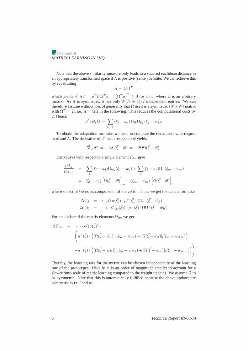
Note that the above similarity measure only leads to a squared euclidean distance inan appropriately transformed space ifΛ is positive (semi-) definite. We can achieve thisby substituting

Λ = Ω ΩT

which yields~uT Λ~u = ~uT Ω ΩT ~u =(

ΩT u)2 ≥ 0 for all ~u, whereΩ is an arbitrary

matrix. As Λ is symmetric, it has onlyN(N + 1)/2 independent entries. We cantherefore assume without loss of generality thatΩ itself is a symmetric(N ×N) matrixwith ΩT = Ω, i.e. Λ = ΩΩ in the following. This reduces the computational costs by2. Hence

dΛ(~w, ~ξ) =∑

i,j,k

(ξi − wi)ΩikΩkj (ξj − wj).

To obtain the adaptation formulas we need to compute the derivatives with respectto ~w andΛ. The derivative ofdΛ with respect to~w yields

~∇w dΛ = −2Λ (~ξ − ~w) = −2ΩΩ(~ξ − ~w).

Derivatives with respect to a single elementΩlm give

∂dΛ

∂Ωlm=

∑

j

(ξl − wl)Ωmj(ξj − wj) +∑

i

(ξi − wi)Ωil(ξm − wm)

= (ξl − wl)[

Ω(~ξ − ~w)]

m+ (ξm − wm)

[

Ω(~ξ − ~w)]

l

where subscriptl denotes componentl of the vector. Thus, we get the update formulas

∆~wJ = ǫ · φ′(µ(~ξ)) · µ+(~ξ) · ΩΩ · (~ξ − ~wJ )

∆~wK = − ǫ · φ′(µ(~ξ)) · µ−(~ξ) · ΩΩ · (~ξ − ~wK)

For the update of the matrix elementsΩlm we get

∆Ωlm = − ǫ · φ′(µ(~ξ)) ·(

µ+(~ξ) ·(

[Ω(~ξ − ~wJ )]m(ξl − wJ,l) + [Ω(~ξ − ~wJ )]l(ξm − wJ,m))

−µ−(~ξ) ·(

[Ω(~ξ − ~wK)]m(ξl − wK,l) + [Ω(~ξ − ~wK)]l(ξm − wK,m))

)

Thereby, the learning rate for the metric can be chosen independently of the learningrate of the prototypes. Usually, it is an order of magnitude smaller to account for aslower time-scale of metric learning compared to the weightupdates. We assumeΩ tobe symmetric. Note that this is automatically fulfilled because the above updates aresymmetric w.r.t.l andm.


Generalization ability

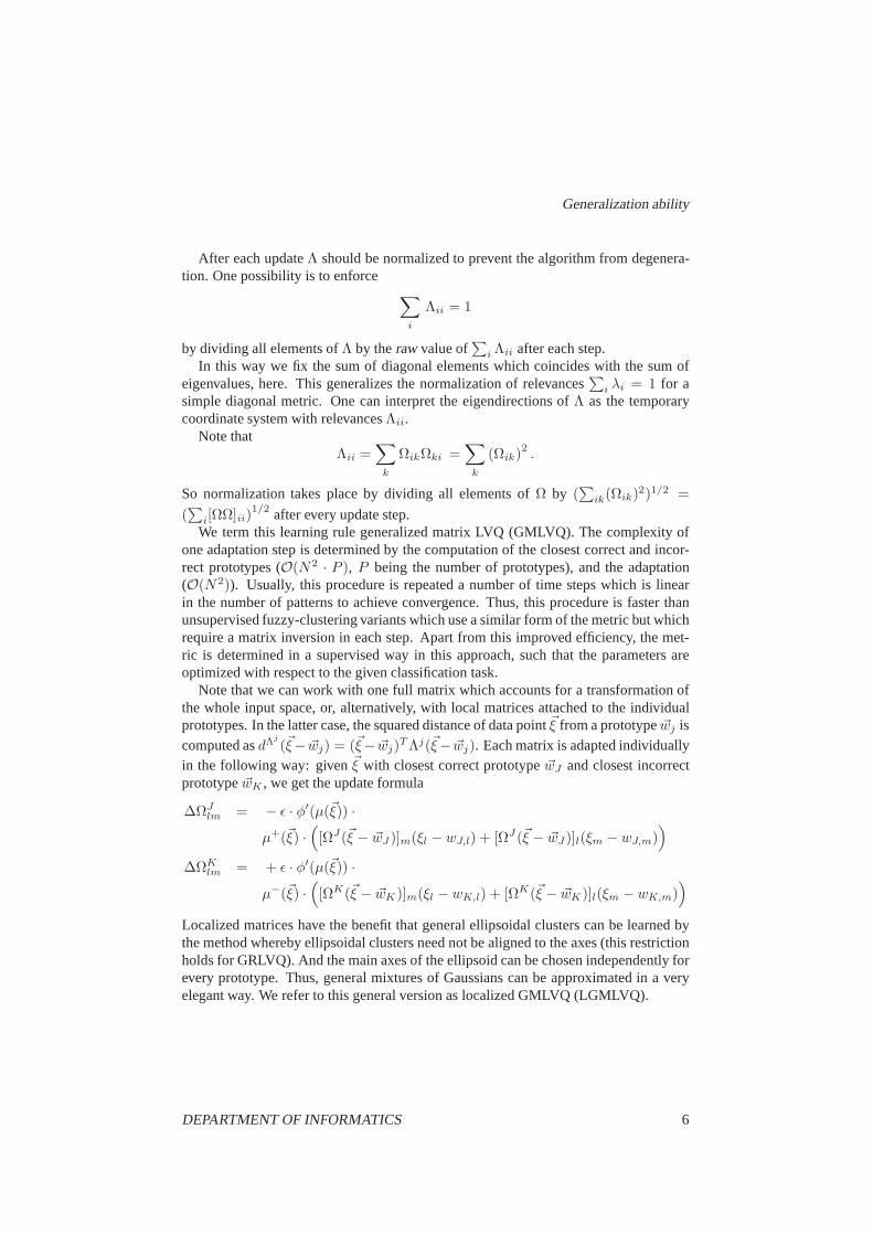
After each updateΛ should be normalized to prevent the algorithm from degenera-tion. One possibility is to enforce

∑

i

Λii = 1

by dividing all elements ofΛ by therawvalue of∑

i Λii after each step.In this way we fix the sum of diagonal elements which coincideswith the sum of

eigenvalues, here. This generalizes the normalization of relevances∑

i λi = 1 for asimple diagonal metric. One can interpret the eigendirections ofΛ as the temporarycoordinate system with relevancesΛii.

Note thatΛii =

∑

k

ΩikΩki =∑

k

(Ωik)2 .

So normalization takes place by dividing all elements ofΩ by (∑

ik(Ωik)2)1/2 =

(∑

i[ΩΩ]ii)1/2 after every update step.

We term this learning rule generalized matrix LVQ (GMLVQ). The complexity ofone adaptation step is determined by the computation of the closest correct and incor-rect prototypes (O(N2 · P ), P being the number of prototypes), and the adaptation(O(N2)). Usually, this procedure is repeated a number of time stepswhich is linearin the number of patterns to achieve convergence. Thus, thisprocedure is faster thanunsupervised fuzzy-clustering variants which use a similar form of the metric but whichrequire a matrix inversion in each step. Apart from this improved efficiency, the met-ric is determined in a supervised way in this approach, such that the parameters areoptimized with respect to the given classification task.

Note that we can work with one full matrix which accounts for atransformation ofthe whole input space, or, alternatively, with local matrices attached to the individualprototypes. In the latter case, the squared distance of datapoint~ξ from a prototype~wj iscomputed asdΛ

j

(~ξ− ~wj) = (~ξ− ~wj)T Λj(~ξ− ~wj). Each matrix is adapted individually

in the following way: given~ξ with closest correct prototype~wJ and closest incorrectprototype~wK , we get the update formula

∆ΩJlm = − ǫ · φ′(µ(~ξ)) ·

µ+(~ξ) ·(

[ΩJ(~ξ − ~wJ )]m(ξl − wJ,l) + [ΩJ (~ξ − ~wJ )]l(ξm − wJ,m))

∆ΩKlm = + ǫ · φ′(µ(~ξ)) ·

µ−(~ξ) ·(

[ΩK(~ξ − ~wK)]m(ξl − wK,l) + [ΩK(~ξ − ~wK)]l(ξm − wK,m))

Localized matrices have the benefit that general ellipsoidal clusters can be learned bythe method whereby ellipsoidal clusters need not be alignedto the axes (this restrictionholds for GRLVQ). And the main axes of the ellipsoid can be chosen independently forevery prototype. Thus, general mixtures of Gaussians can beapproximated in a veryelegant way. We refer to this general version as localized GMLVQ (LGMLVQ).



4 Generalization ability

One of the benefits of prototype-based learning algorithms consists in the fact that theyshow very good generalization ability also for high dimensional data. This observa-tion can be accompanied by theoretical guarantees. It has been shown in [5] that basicLVQ-networks equipped with the euclidean metric possess dimensionality independentlarge-margin generalization bounds, whereby the margin refers to the security of theclassification, i.e. the minimum difference of the distances computed for classification.A similar result has been derived in [11] for LVQ-networks asconsidered above whichpossess an adaptive diagonal metric. Remarkably, the margin is thereby directly cor-related to the nominator of the cost function as introduced above, i.e. these learningalgorithms inherently aim at margin optimization during training. As pointed out in[12], these results transfer immediately to kernelized versions of this algorithm wherethe similarity measure can be interpreted as the composition of the standard scaled eu-clidean metric and a fixed kernel map. In the case of an adaptive full matrix, however,these results are not applicable, because the matrix is changed during training, i.e. thekernel is optimized according to the given classification task in this setting.

Here, we directly derive a large margin generalization bound for (localized) GMLVQnetworks with a full adaptive matrix attached to every prototype, whereby we use theideas of [11]. We consider a LGMLVQ network given byP prototypes~wi with inputs|~ξ| ≤ B for someB > 0 and the case of a binary classification. That means, prototypesc(~wi) are labeled by1 or−1. Classification takes place by a winner takes all rule, i.e.

~ξ 7→ c(~wi) where(~ξ − ~wi)T Λi(~ξ − ~wi) ≤ (~ξ − ~wj)

T Λj(~ξ − ~wj)∀j 6= i (1)

with positive semidefinite matrixΛi with normalization∑

l Λill = 1. The network

corresponds to a function in the class

F := f : RN → −1, 1 | f is given by formula (1) for someΛi, ~wi

We can assume that prototypes are located within the data points, i.e.|~wi| ≤ B.Assume some unknown underlying probability measureP is given onRN×−1, 1.

The goal of learning is to find a functionf ∈ F such that the generalization error

EP (f) := P (y 6= f(y))

is as small as possible. However,P is not known during training; instead, examplesfor the distribution(~ξi, yi), i = 1, . . . , m, are available, which are independent andidentically distributed according toP . Training aims at minimizing the empirical error

Em(f) :=

m∑

i=1

|yi 6= f(~ξi)|/m .

Thus, the learning algorithm generalizes to unseen data ifEm(f) becomes representa-tive for EP (f) for an increasing number of examplesm with high probability.


Generalization ability

The training algorithm of LGMLVQ optimizes a cost function which is correlated tothe number of misclassifications of training. Assume a pattern (~ξ, y) is classified by aGMLVQ network which implements the functionf . We define the margin

Mf (~ξ, y) = −dΛJ

J + dΛK

K

wherebydΛJ

J refers to the distance from the closest prototype with classy anddΛK

K

refers to the distance from the closest prototype with classdifferent fromy. Note thatLGMLVQ tries to maximize this margin during training since it occurs as nominatorwithin the cost function. Following the approach [1], we define the loss function

L : R → R, t 7→

1 if t ≤ 01 − t/ρ if 0 < t ≤ ρ0 otherwise

whereρ > 0 is some fixed value. The term

ELm(f) :=

m∑

i=1

L(Mf(~ξi, yi))/m

accumulates the number of errors for a given data set, and, inaddition, also punishesall correct classifications with a margin smaller thanρ.

It is possible to correlate the generalization error and this modified empirical errorby a dimensionality independent bound. According to [1](Theorem 7) for allf ∈ Fwith probability at least1 − δ/2, the inequality

EP (f) ≤ ELm(f) +

2K

ρ· Gm(F) +

√

ln(4/δ)

2m

holds, wherebyK is a universal constant andGm(F) is the Gaussian complexity whichis the expectation of the quantity

Eg1,...,gm

(

supf∈F

∣

∣

∣

∣

∣

2

m

m∑

i=1

gi · f(~ξi)

∣

∣

∣

∣

∣

)

with respect to the patterns~ξi wheregi constitute independent Gaussian variables withzero mean and unit variance. It measures the amount of surprise in the consideredfunction class.

A winner-takes-all classification according to equation (1) can be formulated asBoolean formula over terms of the formdΛ

i

i −dΛj

j wherei andj enumerate the mutuallydifferent prototypes. There existP (P − 1)/2 such pairs. According to [1](Theorem16), we find

Gm(F) ≤ P (P − 1) · Gm(Fij)



wherebyFij denotes a LGMLVQ network with only two prototypes. For a networkwith two prototypes, we get for input~ξ

dΛi − dΛ

j

j ≤ 0

⇐⇒ ~ξT Λi~ξ − ~ξT Λj~ξ −2(~wT

i Λi − ~wTj Λj)~ξ + (~wi)

T Λi ~wi + (~wj)T Λj ~wj ≤ 0

This is the sum of a linear classifier and a quadratic term. Adding a constant inputdimension1 to ~ξ, the input to the linear classifier is restricted byB + 1 and the lengthof the weight vector is restricted by4B + 2B2 because vectors|~wi| are limited byBand the sum of the eigenvalues ofΛi is at most1. The empirical Gaussian complexityof this linear part is limited by

4B(B + 1)(B + 2)√

m

m

according to [1](Lemma 22). According to the same theorem, the Gaussian complexityof the quadratic term is limited by

4 · B · √m

m.

Thus, an overall estimation is given by the sum of these termswhich is of orderB3/√

m.Since the empirical Gaussian complexity and the Gaussian complexity differ by more

thanǫ with probability at most2 exp(−ǫ2m/8) according to [1](Theorem 11), i.e. theydiffer by no more than

√

8/m · ln(4/δ) with probability at least1− δ/2, we finally get

EP (f) ≤ ELm(f) + O

(

1√m

·(

P 2B3

ρ+

P 2√

ln(1/δ)

ρ+√

ln(1/δ)

))

(2)

with probability1 − δ. This bound is independent of the dimensionality of the data.Rather, it involves the marginρ which is directly optimized during GMLVQ training.

This bound holds for priorly fixed marginρ. For posterior marginρ, a generalizationof the argumentation as follows can be applied: Assume the empirical margin can beupper bounded byC > 0, a naive bound being e.g. the maximum distance of data in thegiven training set. We defineρi = C/i for i ≥ 1, and we choose prior probabilitiespi ≥0 with

∑

pi = 1 which indicate the confidence in achieving an empirical margin of sizeρi. Define the cost functionLi as above associated to marginρi and the correspondingempirical errorELi

m (f). We are interested in the probability

P(

∃i EP (f) ≥ ELi

m (f) + ǫ(i))


Experiments

where the bound

ǫ(i) =

(

K ′

√m

·(

P 2B3

ρi+

P 2√

ln(1/(piδ))

ρi+√

ln(1/(piδ))

))

depends on the empirical margin,K ′ being a constant. We can argue

P(

∃i EP (f) ≥ ELim (f) + ǫ(i)

)

≤∑

i

P(

EP (f) ≥ ELim (f) + ǫ(i)

)

≤∑

i

pi · δ = δ

because the boundsǫ(i) are chosen according to equation (2). Thus, posterior boundsdepending on the empirical margin and the prior confidence inachieving this margincan be derived.

5 Experiments

We test the performance of GMLVQ in comparison to GRLVQ and GLVQ without met-ric adaptation using an artificial data set and the image segmentation data set providedin the UCI repository [15].

5.1 Artificial Data

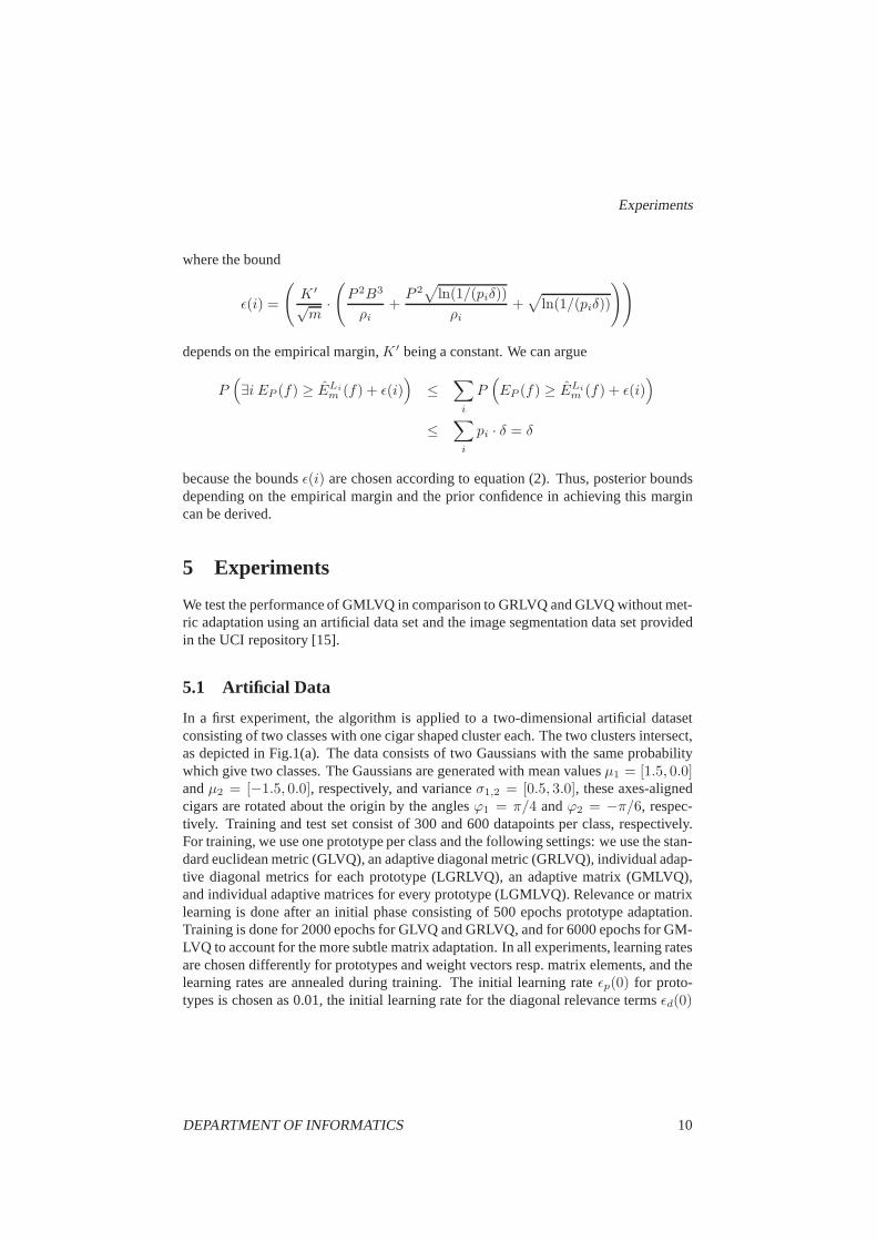
In a first experiment, the algorithm is applied to a two-dimensional artificial datasetconsisting of two classes with one cigar shaped cluster each. The two clusters intersect,as depicted in Fig.1(a). The data consists of two Gaussians with the same probabilitywhich give two classes. The Gaussians are generated with mean valuesµ1 = [1.5, 0.0]andµ2 = [−1.5, 0.0], respectively, and varianceσ1,2 = [0.5, 3.0], these axes-alignedcigars are rotated about the origin by the anglesϕ1 = π/4 andϕ2 = −π/6, respec-tively. Training and test set consist of 300 and 600 datapoints per class, respectively.For training, we use one prototype per class and the following settings: we use the stan-dard euclidean metric (GLVQ), an adaptive diagonal metric (GRLVQ), individual adap-tive diagonal metrics for each prototype (LGRLVQ), an adaptive matrix (GMLVQ),and individual adaptive matrices for every prototype (LGMLVQ). Relevance or matrixlearning is done after an initial phase consisting of 500 epochs prototype adaptation.Training is done for 2000 epochs for GLVQ and GRLVQ, and for 6000 epochs for GM-LVQ to account for the more subtle matrix adaptation. In all experiments, learning ratesare chosen differently for prototypes and weight vectors resp. matrix elements, and thelearning rates are annealed during training. The initial learning rateǫp(0) for proto-types is chosen as 0.01, the initial learning rate for the diagonal relevance termsǫd(0)



Table 1: (a): Percentage of correctly classified patters forthe artificial training and testset using the different LVQ-algorithms. (b): Percentage ofcorrectly classified patternsfor image data on training and test set.

(a)

Algorithm Training TestGLVQ 75.33 71.83

GRLVQ 74.33 72.33GMLVQ 79.67 77.83LGRLVQ 81.0 78.0LGMLVQ 91.67 90.75

(b)

Algorithm Training TestGLVQ 82.38 79.05

GRLVQ 85.71 84.52GMLVQ 91.9 87.86LGRLVQ 90.0 89.05LGMLVQ 96.19 94.29

is chosen as 0.005 and the initial learning rate for nondiagonal matrix elementsǫm(0)is chosen as0.0001. For annealing, we use the following learning rate schedules:

ǫ(t) =ǫ(0)

1 + τ · (t − tstart)

wheretstart denotes the starting epoch for the adaptation, i.e. it is 1 for the weightadaptation and 500 for the adaptation of matrix elements andrelevance factors. Theparameterτ is chosen as 0.0001.

The classification accuracies on the training and test set are summarized in Tab.1(a).The position of the resulting prototypes and decision boundaries are shown in Fig.1(b)-(f). GMLVQ determines one single direction in feature space, which is used for classifi-cation. The resulting matrixΩ projects the data onto the respective subspace as depictedin Fig.1(g), Fig.1(h) denotes the projections of the classes using the LGMLVQ matrices

ΛClass1 =

(

0.5156 −0.4997−0.4997 0.4844

)

ΛClass2 =

(

0.7195 0.44920.4492 0.2805

)

One can clearly observe the benefit of individual matrix adaptation: this allows eachprototype to shape its cluster according to the local ellipsoidal form of the class. Thisway, the data points of both cigar shaped clusters can be classified correctly exceptfor the tiny region where the classes overlap. Note that, forlocal metric parameteradaptation, the receptive fields of the prototypes are no longer separated by straightlines (see Fig. 1(d)) and, further, need no longer be convex in this case (see Fig. 1(f)).

5.2 Image Data

In a second experiment, the algorithm was applied to the image segmentation datasetprovided in the UCI repository [15]. The dataset contains 19dimensional feature vec-tors, which encode different attributes of 3x3 Pixel regions extracted out of seven out-door images (brickface, sky, foliage, cement, window, path, grass). The features 3-5 are


Experiments

−5 0 5

−10

−5

0

5

Class 1Class 2

(a)

−5 0 5

−10

−5

0

5

Class 1Class 2

(b)

−5 0 5

−10

−5

0

5

Class 1Class 2

(c)

−5 0 5

−10

−5

0

5

Class 1Class 2

(d)

−5 0 5

−10

−5

0

5

Class 1Class 2

(e)

−5 0 5

−10

−5

0

5

Class 1Class 2

(f)

−5 0 5

−10

−5

0

5

Class 1Class 2

(g)

−5 0 5

−10

−5

0

5

Class 1Class 2

(h)

Figure 1: (a): Artificial dataset used for training. (b)-(f)Position of prototypes and deci-sion boundaries after training with different LVQ-algorithms. (b):GLVQ, (c):GRLVQ,(d):LGRLVQ, (e):GMLVQ, (f):LGMLVQ, (g):data transformedby global matrixΩ,(h): data transformed by individual matrices for both prototypes.

(nearly) constant and were eliminated for this experiment.The training set consists of210 datapoints (30 per class), the test sets contains 300 datapoints per class.

As beforehand, we used one prototype per class. In all experiments, the adaptationof metric parameters starts after an initial training phasefor the prototypes consisting ofa few 100 epochs. As beforehand, we compare global and local relevance resp. matrixadaptation and simple GLVQ. The initial learning rates havebeen optimized on thetraining set and they are chosen as follows:

• GLVQ: ǫp(0) = 0.8

• GRLVQ: ǫp(0) = 0.8, ǫd(0) = 5 · 10−6

• LGRLVQ: ǫd(0) = 5 · 10−5

• GMLVQ: ǫp(0) = 0.8, ǫd(0) = 1 · 10−4, ǫm(0) = 5 · 10−5

• LGMLVQ: ǫp(0) = 0.8, ǫd(0) = 1 · 10−3, ǫm(0) = 5 · 10−5

These learning rates are annealed as beforehand usingτ = 0.001.



1 2 3 4 5 6 7 8 9 10 11 12 13 14 15 160

0.1

0.2

0.3

0.4

0.5

2 4 6 8 10 12 14 16

2

4

6

8

10

12

14

16

−0.08

−0.06

−0.04

−0.02

0

0.02

0.04

0.06

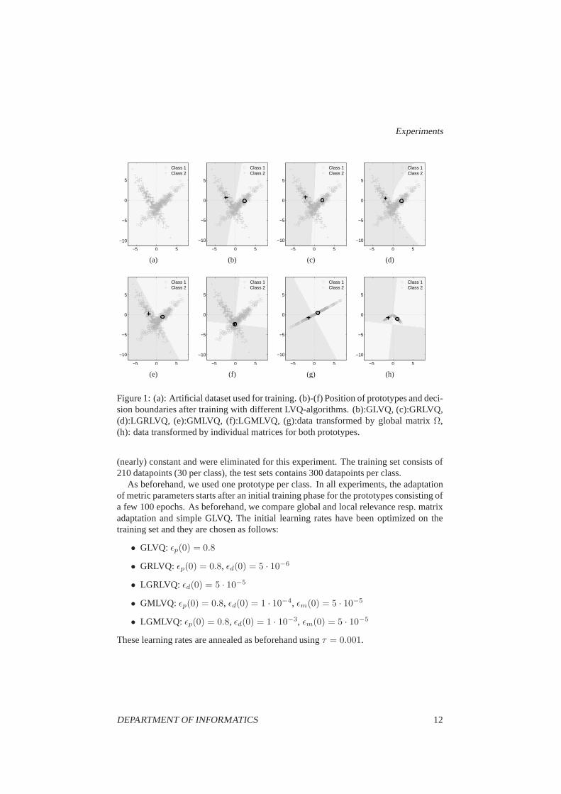
Figure 2: Visualization of the final relevance matrix for brickface-class. Left: diagonalelements. Right: nondiagonal elements

1 2 3 4 5 6 7 8 9 10 11 12 13 14 15 160

0.1

0.2

0.3

0.4

0.5

2 4 6 8 10 12 14 16

2

4

6

8

10

12

14

16

−0.08

−0.06

−0.04

−0.02

0

0.02

0.04

0.06

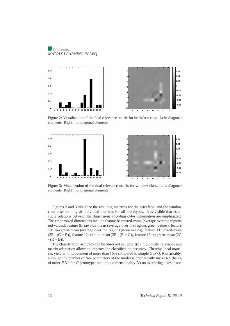
Figure 3: Visualization of the final relevance matrix for window-class. Left: diagonalelements. Right: nondiagonal elements

Figures 2 and 3 visualize the resulting matrices for the brickface- and the windowclass after training of individual matrices for all prototypes. It is visible that espe-cially relations between the dimensions encoding color information are emphasized:The emphasized dimensions include feature 8: rawred-mean (average over the regionsred values), feature 9: rawblue-mean (average over the regions green values), feature10: rawgreen-mean (average over the regions green values),feature 11: exred-mean(2R - (G + B)), feature 12: exblue-mean (2B - (R + G)), feature 13: exgreen-mean (2G- (R + B)).

The classification accuracy can be observed in Table 1(b). Obviously, relevance andmatrix adaptation allows to improve the classification accuracy. Thereby, local matri-ces yield an improvement of more than 10% compared to simple GLVQ. Remarkably,although the number of free parameters of the model is dramatically increased (beingof orderPN2 for P prototypes and input dimensionalityN ) no overfitting takes place.


References

This demonstrates the good generalization ability of the model as substantiated by theformal generalization bounds.

6 Discussion

We have extended GRLVQ, a particularly efficient and powerful prototype based classi-fier, by a full matrix adaptation scheme. This allows the adaptation of the class borderssuch that local ellipsoidal shapes are taken into account. The possibility to improvethe classification accuracy by this extension has been demonstrated in two examples.Remarkably, the generalization ability of the method is quite high as substantiated bytheoretical findings.

The complexity of full local matrix adaptations scales withN2 per epoch,N beingthe input dimensionality. This is better than comparable matrix adaptation methods asused e.g. in unsupervised fuzzy clustering [7, 9], however,the computational load be-comes quite large for large input dimensionality. Therefore, specific schemes to shapethe form of the matrix based on prior information are of particular interest. Nondiagonalmatrix elements indicate a correlation of input features relevant for the classification. Inmany cases, one can restrict useful correlations due to prior knowledge. As an example,spatial or temporal data likely sho a high correlation of neighbored elements, whereasthe other elements are probably independent. In such cases,one can restrict to a fixedadaptive bandwidth, decreasing the quadratic complexity to a linear term with respectto input dimensionality. Similarly, spatial correlationsin images or functional data canlead to a massive restriction of the free parameters of the matrices to promising regions.This possibility will be the subject of future experiments.

References

[1] P.L. Bartlett and S. Mendelson. Rademacher and Gaussiancomplexities: riskbounds and structural risks.Journal of Machine Learning Research3:463–4812,2002.

[2] M. Biehl, A. Ghosh, and B. Hammer. Learning vector quantization: The dynamicsof winner-takes-all algorithms,Neurocomputing69(7-9):660-670, 2006.

[3] M. Biehl, A. Ghosh, and B. Hammer. Dynamics and generalization ability of LVQalgorithms, to appear inJournal of Machine Learning Research, 2006.

[4] Bibliography on the Self-Organizing Map (SOM) and LearningVector Quantiza-tion (LVQ), Neural Networks Research Centre, Helsinki University of Technology,2002.

[5] K. Crammer, R. Gilad-Bachrach, A. Navot, and A. Tishby. Margin analysis of theLVQ algorithm. InAdvances of Neural Information Processing Systems, 2002.



[6] R. Duda, P. Hart, and D. Storck.Pattern Classification, Wiley, 2001.

[7] I. Gath and A.B. Geva. Unsupervised optimal fuzzy clustering. IEEE Transactionson Pattern Analysis and Machine Intelligence11:773–781, 1989.

[8] A. Ghosh, M. Biehl, and B. Hammer. Performance analysis of LVQ algorithms: astatistical physics approach,Neural Networks19:817-829, 2006.

[9] E.E. Gustafson and W.C. Kessel. Fuzzy clustering with a fuzzy covariance matrix.IEEE CDC, pages 761–766, San Diego, California, 1979.

[10] B. Hammer, F.-M. Schleif, and T. Villmann. On the Generalization Ability ofPrototype-Based Classifiers with Local Relevance Determination, Technical Re-port, Clausthal University of Technology, Ifi-05-14, 2005.

[11] B. Hammer, M. Strickert, and T. Villmann. On the generalization ability of GR-LVQ networks.Neural Processing Letters21(2):109–120, 2005.

[12] B. Hammer, M. Strickert, and T. Villmann. Supervised neural gas with generalsimilarity measure.Neural Processing Letters21(1): 21–44, 2005.

[13] B. Hammer and T. Villmann,Generalized relevance learning vector quantization,Neural Networks 15: 1059-1068, 2002.

[14] T. Kohonen,Self-organizing maps, Springer, Berlin, 1995.

[15] D.J.Newman, S.Hettich, C.L.Blake, C.J.Merz.UCI Repository of machine learn-ing databases[http://www.ics.uci.edu/ mlearn/MLRepository.html]. Irvine, CA:University of California, Department of Information and Computer Science, 1998.

[16] A.S. Sato and K. Yamada. Generalized learning vector quantization. InG. Tesauro, D. Touretzky, and T. Leen (eds.),Advances in Neural InformationProcessing Systems, volume 7, pages 423–429, MIT Press, 1995.

[17] S. Seo, M. Bode, and K. Obermayer,Soft nearest prototype classification, IEEETransactions on Neural Networks 14(2): 390-398, 2003.

[18] S. Seo and K. Obermayer,Soft Learning Vector Quantization. Neural Computa-tion 15(7): 1589-1604, 2003.


Matrix Learning in Learning Vector Quantization · Matrix Learning in Learning Vector Quantization...

Documents

Transcript of Matrix Learning in Learning Vector Quantization · Matrix Learning in Learning Vector Quantization...