matrices and algbra
82
1 Linear Algebra
-
Upload
jitendra-thakor -
Category
Education
-
view
229 -
download
0
Transcript of matrices and algbra

1
Linear Algebra

Systems of Linear Equation and Matrices
CHAPTER 1
FASILKOM UI 05

Linear Algebra - Chapter 1 [YR2005] 3
Introduction ~ Matrices
Information in science and mathematics is often organized into rows and columns to form rectangular arrays.
Tables of numerical data that arise from physical observations
Example: (to solve linear equations)
Solution is obtained by performing appropriate operations on this matrix
− 412
315
42
35
=−=+yx
yx

1.1 Introduction to
Systems of Linear Equations
Linear Algebra - Chapter 1 [YR2005] 5
Linear Equations
In x y variables (straight line in the xy-plane)
where a1, a2, & b are real constants,
In n variables
where a1, …, an & b are real constants
x1, …, xn = unknowns.
Example 1 Linear Equations
The equations are linear (does not involve any products or roots of variables).
byaxa =+ 21
bxaxaxa nn =+++ ...2211
73 =+ yx 1321 ++= zxy 732 4321 =+−− xxxx

Linear Algebra - Chapter 1 [YR2005] 6
Linear Equations
The equations are not linear. A solution of is a sequence
of n numbers s1, s2, ..., sn Э they satisfy the equation when x1=s1, x2=s2, ..., xn=sn (solution set).
Example 2 Finding a Solution Set
1 equation and 2 unknown, set one var as the parameter (assign any value)
or
1 equation and 3 unknown, set 2 vars as parameter
53 =+ yx 423 =+−+ xzzyx xy sin=
bxaxaxa nn =+++ ...2211
124 =− yx
212, −== tytx tytx =+= ,4
121
574 321 =+− xxx
txsxtsx ==−+= 321 ,,745

Linear Algebra - Chapter 1 [YR2005] 7
Linear Systems / System of Linear Equations Is A finite set of linear equations in the vars x1, ..., xn
s1, ..., sn is called a solution if x1=s1, ..., xn=sn is a solution of every equation in the system.
Ex.
x1=1, x2=2, x3=-1 the solution
x1=1, x2=8, x3=1 is not, satisfy only the first eq.
System that has no solution : inconsistent System that has at least one solution: consistent
Consider:
493
134
321
321
−=++−=+−
xxx
xxx
00,:
00,:
112222
111111
≠∧≠=+≠∧≠=+bacybxal
bacybxal

Linear Algebra - Chapter 1 [YR2005] 8
(x,y) lies on a line if and only if the numbers x and y satisfy the equation of the line. Solution: points of intersection l1 & l2
l1 and l2 may be parallel:
no intersection, no solution
l1 and l2 may intersect
at only one point: one solution
l1 and l2 may coincide:
infinite many points of intersection, infinitely many solutions
Linear Systems
x
x
y1l 2l
x
y
x
y
1l 2l
21 & ll
Linear Algebra - Chapter 1 [YR2005] 9
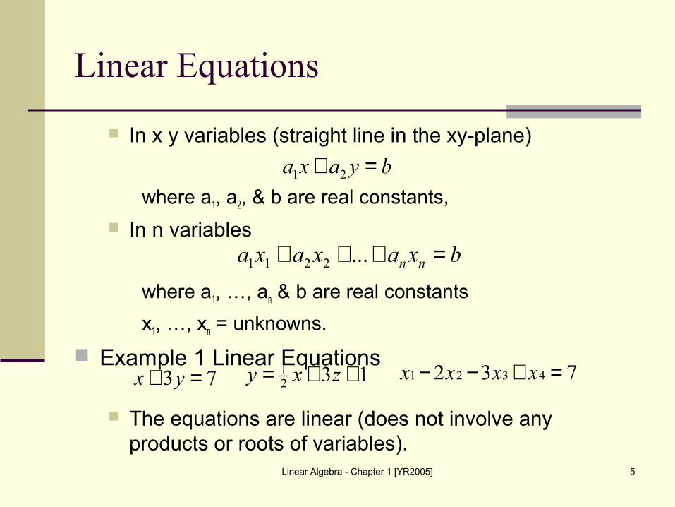
Linear Systems
In general: Every system of linear equations has either no solutions, exactly one solution, or infinitely many solutions.
An arbitrary system of m linear equations in n unknowns:a11x1 + a12x2 + ... + a1nxn = b1
a21x1 + a22x2 + ... + a2nxn = b2
am1x1 + am2x2 + ... + amnxn = bm
x1, ..., xn = unknowns, a’s and b’s are constants aij, i indicates the equation in which the coefficient
occurs and j indicates which unknown it multiplies

Linear Algebra - Chapter 1 [YR2005] 10
Augmented Matrices
Example:
Remark: when constructing, the unknowns must be written in the same order in each equation and the constants must be on the right.
mmnmm
n
n
baaa
baaa
baaa
21
222221
111211
0563
1342
92
321
321
321
=−+=−+
=++
xxx
xxx
xxx
−−
0563
1342
9211

Linear Algebra - Chapter 1 [YR2005] 11
Augmented Matrices
Basic method of solving system linear equations Step 1: multiply an equation through by a nonzero
constant. Step 2: interchange two equations. Step 3: add a multiple of one equation to another.
On the augmented matrix (elementary row operations): Step 1: multiply a row through by a nonzero
constant. Step 2: interchange two rows. Step 3: add a multiple of one equation to another.

Linear Algebra - Chapter 1 [YR2005] 12
Elementary Row Operations (Example)
r2= -2r1 + r2
r3 = -3r1 + r3
0563:
1772:
92:
3
2
1
=−+−=−=++
zyxr
zyr
zyxr
0563:
1342:
92:
3
2
1
=−+=−+
=++
zyxr
zyxr
zyxr
−−
0563
1342
9211
−−−
0563
17720
9211
27113:
1772:
92:
3
2
1
−=−−=−=++
zyr
zyr
zyxr
−−−−
271130
17720
9211

Linear Algebra - Chapter 1 [YR2005] 13
Elementary Row Operations (Example) r2 = ½ r2
r3 = -3r2 + r3
r3 = -2r3
27113:
:
92:
3
217
27
2
1
−=−−=−=++
zyr
zyr
zyxr
−−−−
271130
10
9211
217
27
23
21
3
217
27
2
1
:
:
92:
−=−−=−=++
zr
zyr
zyxr
−−−−
23
21
217
27
00
10
9211
3:
:
92:
3
217
27
2
1
=−=−=++
zr
zyr
zyxr7 172 2
1 1 2 9
0 1
0 0 1 3
− −

Linear Algebra - Chapter 1 [YR2005] 14
Elementary Row Operations (Example) r1 = r1 – r2
r1 = -11/2 r3 + r1
r2 = 7/2 r3 + r2
Solution:
3:
:
:
3
217
27
2
235
211
1
=−=−
=+
zr
zyr
zxr
−−3100
10
01
217
27
235
211
3100
2010
1001
3:
2:
1:
3
2
1
===
zr
yr
xr3:
:
1:
3
217
27
2
1
=−=−
=
zr
zyr
xr
−−3100
10
1001
217
27

1.2 Gaussian Elimination

Linear Algebra - Chapter 1 [YR2005] 16
Echelon Forms
Reduced row-echelon form, a matrix must have the following properties: If a row does not consist entirely of zeros the the
first nonzero number in the row is a 1 = leading 1 If there are any rows that consist entirely of zeros,
then they are grouped together at the bottom of the matrix.
In any two successive rows that do not consist entirely of zeros, the leading 1 in the lower row occurs farther to the right than the leading 1 in the higher row.
Each column that contains a leading 1 has zeros everywhere else.

Linear Algebra - Chapter 1 [YR2005] 17
Echelon Forms
A matrix that has the first three properties is said to be in row-echelon form.
Example: Reduced row-echelon form:
Row-echelon form:
−
−00
00,
00000
00000
31000
10210
,
100
010
001
,
1100
7010
4001
1 4 3 7 1 1 0 0 1 2 6 0
0 1 6 2 , 0 1 0 , 0 0 1 1 0
0 0 1 5 0 0 0 0 0 0 0 1
− −
Linear Algebra - Chapter 1 [YR2005] 18
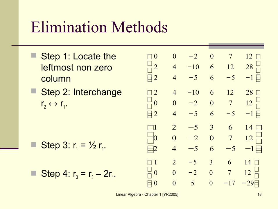
Elimination Methods
Step 1: Locate the leftmost non zero column
Step 2: Interchange r2 ↔ r1.
Step 3: r1 = ½ r1.
Step 4: r3 = r3 – 2r1.
−−−−−
156542
281261042
1270200
−−−−−
156542
1270200
281261042
−−−−−
156542
1270200
1463521
−−−−
29170500
1270200
1463521

Linear Algebra - Chapter 1 [YR2005] 19
Elimination Methods
Step 5 : continue do all steps above until the entire matrix is in row-echelon form.
r2 = -½ r2
r3 = r3 – 5r2
r3 = 2r3
−−−−
−
29170500
60100
1463521
27
−−
−
10000
60100
1463521
21
27
−−
−
210000
60100
1463521
27

Linear Algebra - Chapter 1 [YR2005] 20
Elimination Methods
Step 6 : add suitable multiplies of each row to the rows above to introduce zeros above the leading 1’s.
r2 = 7/2 r3 + r2
r1 = -6r3 + r1
r1 = 5r2 + r1
−
210000
100100
1463521
−
210000
100100
203521
210000
100100
703021

Linear Algebra - Chapter 1 [YR2005] 21
Elimination Methods
1-5 steps produce a row-echelon form (Gaussian Elimination). Step 6 is producing a reduced row-echelon (Gauss-Jordan Elimination).
Remark: Every matrix has a unique reduced row-echelon form, no matter how the row operations are varied. Row-echelon form of matrix is not unique: different sequences of row operations can produce different row- echelon forms.

Linear Algebra - Chapter 1 [YR2005] 22
Back-substitution
Bring the augmented matrix into row-echelon form only and then solve the corresponding system of equations by back-substitution.
Example: [Solved by back substitution]
−
0000000
100000
1302100
0020231
31
31
6
643
5321
132
0223
==++=+−+
x
xxx
xxxx
31
6
643
5321
321
223 1. Step
=−−=
−+−=
x
xxx
xxxx

Linear Algebra - Chapter 1 [YR2005] 23
Back-Substitution
31
6
43
5421
43
31
6
43
5321
31
6
2
243
2 ngSubstituti
2
223
ngSubstituti
2. Step
=−=
−−−=−=
=−=
−+−==
x
xx
xxxx
xx
x
xx
xxxx
x
Step 3. Assign arbitrary values to the free variables [parameters], if any
31
6
5
4
3
2
1
2
243
===
−==
−−−=
x
tx
sx
sx
rx
tsrx

Linear Algebra - Chapter 1 [YR2005] 24
Homogeneous Linear Systems
A system of linear equations is said to be homogeneous if the constant terms are all zero.
Every homogeneous sytem of linear equations is consistent, since all such systems have x1=0,x2=0,...,xn=0 as a solution [trivial solution]. Other solutions are called nontrivial solutions.
01
0
0
221
2222121
1212111
=+++
=+++=+++
nmnmm
nn
nn
xaxaxa
xaxaxa
xaxaxa

Linear Algebra - Chapter 1 [YR2005] 25
Homogeneous Linear Systems
Example: [Gauss-Jordan Elimination]
0
02
032
022
543
5321
54321
5321
=++=−−+=+−+−−=+−+
xxx
xxxx
xxxxx
xxxx
⇒
−−−−−
−
000000
001000
010100
010011
011100
010211
013211
010122
Linear Algebra - Chapter 1 [YR2005] 26
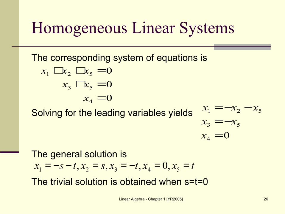
Homogeneous Linear Systems
The corresponding system of equations is
Solving for the leading variables yields
The general solution is
The trivial solution is obtained when s=t=0
04
53
521
=−=
−−=
x
xx
xxx0
0
0
4
53
521
==+=++
x
xx
xxx
txxtxsxtsx ==−==−−= 54321 ,0,,,

Linear Algebra - Chapter 1 [YR2005] 27
Homogeneous Linear Systems
Theorem:
A homogeneous system of linear equations with more unknowns than equations has infinitely many solutions.

1.3 Matrices and Matrix Operations

Linear Algebra - Chapter 1 [YR2005] 29
Matrix Notation and Terminology
A matrix is a rectangular array of numbers with rows and columns.
The numbers in the array are called the entries in the matrix.
Examples:
The size of a matrix is described in terms of the number of rows and columns its contains.
A matrix with only one column is called a column matrix or a column vector.
A matrix with only one row is called a row matrix or a row vector.
[ ] [ ]4,3
1,
000
10
2
,3012,
41
03
21
21
−−
−
πe
Linear Algebra - Chapter 1 [YR2005] 30
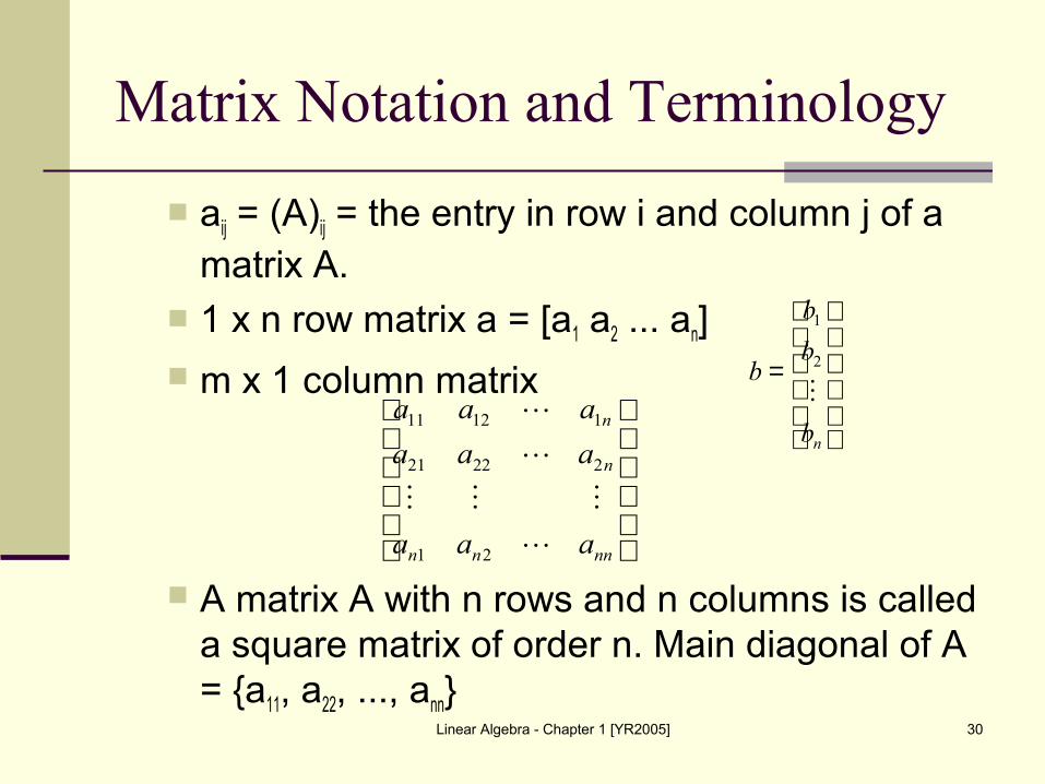
Matrix Notation and Terminology
aij = (A)ij = the entry in row i and column j of a matrix A.
1 x n row matrix a = [a1 a2 ... an]
m x 1 column matrix
A matrix A with n rows and n columns is called a square matrix of order n. Main diagonal of A = {a11, a22, ..., ann}
=
nb
b
b
b2
1
nnnn
n
n
aaa
aaa
aaa
21
22221
11211

Linear Algebra - Chapter 1 [YR2005] 31
Operations on Matrices
Definition: Two matrices are defined to be equal if they have the
same size and their corresponding entries are equal. If A = [aij] and B = [bij] have the same size, then A=B if
and only if (A)ij=(B)ij, or equivalently aij=bij for all i and j.
Definition: If A and B are matrices of the same size, then the sum
A+B is the matrix obtained by adding the entries of B to the corresponding entries of A, and the difference A–B is the matrix obtained by subtracting the entries of B from the corresponding entries of A. Matrices of different sizes cannot be added or subtracted.

Linear Algebra - Chapter 1 [YR2005] 32
Operations on Matrices
If A = [aij] and B = [bij] have the same size, then
(A+B)ij = (A)ij + (B)ij = aij + bij and
(A-B)ij = (A)ij – (B)ij = aij - bij
Definition: If A is any matrix and c is any scalar, then the product
cA is the matrix obtained by multiplying each entry of the matrix A by c. The matrix cA is said to be a scalar multiple of A.
If A = [aij], then (cA)ij = c(A)ij = caij.

Linear Algebra - Chapter 1 [YR2005] 33
Operations on Matrices
Definition
If A is an mxr matrix and B is an rxn matrix, then the product AB is the mxn matrix whose entries are determined as follows. To find the entry in row i and column j of AB, single out row i from the matrix A and column j from the matrix B. Multiply the corresponding entries from the row and column together and then add up the resulting products.

Linear Algebra - Chapter 1 [YR2005] 34
Partitioned Matrices

Linear Algebra - Chapter 1 [YR2005] 35
Matrix Multiplication by Columns and by Rows

Linear Algebra - Chapter 1 [YR2005] 36
Matrix Products as Linear Combinations

Linear Algebra - Chapter 1 [YR2005] 37
Matrix Form of a Linear System

Linear Algebra - Chapter 1 [YR2005] 38
Transpose of a Matrix
1.4 Inverses; Rules of Matrix Arithmetic

Linear Algebra - Chapter 1 [YR2005] 40
Properties of Matrix Operations
ab = ba for real numbers a & b, but AB ≠ BA even if both AB & BA are defined and have the same size.
Example:
−
=
−−=
=
−=
03
63,
411
21
03
21,
32
01
BAAB
BA

Linear Algebra - Chapter 1 [YR2005] 41
Properties of Matrix Operations
Theorem: Properties ofa) A+B = B+A
b) A+(B+C) = (A+B)+C
c) A(BC) = (AB)C
d) A(B+C) = AB+AC
e) (B+C)A = BA+CA
f) A(B-C) = AB-AC
g) (B-C)A = BA-CA
h) a(B+C) = aB+aC
i) a(B-C) = aB-aC
Math Arithmetic(Commutative law for addition)
(Associative law for addition)
(Associative for multiplication)
(Left distributive law)
(Right distributive law)j) (a+b)C = aC+bCk) (a-b)C = aC-bCl) a(bC) = (ab)Cm) a(BC) = (aB)C

Linear Algebra - Chapter 1 [YR2005] 42
Properties of Matrix Operations
Proof (d): Proof for both have the same size:
Let size A be r x m matrix, B & C be m x n (same size).
This makes A(B+C) an r x n matrix, follows that AB+AC is also an r x n matrix.
Proof that corresponding entries are equal: Let A=[aij], B=[bij], C=[cij]
Need to show that [A(B+C)]ij = [AB+AC]ij for all values of i and j.
Use the definitions of matrix addition and matrix multiplication.

Linear Algebra - Chapter 1 [YR2005] 43
Properties of Matrix Operations
Remark: In general, given any sum or any product of matrices, pairs of parentheses can be inserted or deleted anywhere within the expression without affecting the end result.
ij
ijij
mjimjijimjimjiji
mjmjimjjijjiij
ACAB
acAB
cacacabababa
cbacbacbaCBA
][
][][
)()(
)()()()]([
22112211
222111
+=+=
+++++++=++++++=+

Linear Algebra - Chapter 1 [YR2005] 44
Zero Matrices
A matrix, all of whose entries are zero, such as
A zero matrix will be denoted by 0 or 0mxn for the mxn zero matrix. 0 for zero matrix with one column.
Properties of zero matrices: A + 0 = 0 + A = A A – A = 0 0 – A = -A A0 = 0; 0A = 0
[ ]0,
0
0
0
0
,0000
0000,
000
000
000
,00
00

Linear Algebra - Chapter 1 [YR2005] 45
Identity Matrices
Square matrices with 1’s on the main diagonal and 0’s off the main diagonal, such as
Notation: In = n x n identity matrix.
If A = m x n matrix, then: AIn = A and InA = A
1000
0100
0010
0001
,
100
010
001
,10
01

Linear Algebra - Chapter 1 [YR2005] 46
Identity Matrices
Example:
Theorem: If R is the reduced row-echelon form of an n x n matrix A, then either R has a row of zeros or R is the identity matrix In.
=
232221
131211
aaa
aaaA
Aaaa
aaa
aaa
aaaAI =
=
=
232221
131211
232221
1312112
10
01
Aaaa
aaa
aaa
aaaAI =
=
=
232221
131211
232221
1312113
100
010
001

Linear Algebra - Chapter 1 [YR2005] 47
Identity Matrices
Definition: If A & B is a square matrix and same size Э AB = BA = I, then A is said to be invertible and B is called an inverse of A. If no such matrix B can be found, then A is said to be singular.
Example:
−
−=
=
31
52,
21
53AB
IBA
IAB
=
=
−
−
=
=
=
−
−=
10
01
31
52
21
53
10
01
21
53
31
52

Linear Algebra - Chapter 1 [YR2005] 48
Properties of Inverses
Theorem: If B and C are both inverses of the matrix A, then B = C.
If A is invertible, then its inverse will be denoted by the symbol A-1.
The matrix
is invertible if ad-bc ≠ 0, in which case the inverse is given by the formula
=
dc
baA
−−−
−−
−=
−
−−
=−
bcad
a
bcad
cbcad
b
bcad
d
ac
bd
bcadA
11

Linear Algebra - Chapter 1 [YR2005] 49
Properties of Inverses
Theorem: If A and B are invertible matrices of the same size, then AB is invertible and (AB)-1 = B-1A-1.
A product of any number of invertible matrices is invertible, and the inverse of the product is the product of the inverses in the reverse order. Example:
=
=
=
89
67,
22
23,
31
21ABBA
−
−=
−
−=
−
−= −−−
2
7
2
934
)(,1
11,
11
23 1
23
11 ABBA
−
−=
−
−
−
−=−−
2
7
2
934
11
23
1
11
23
11AB

Linear Algebra - Chapter 1 [YR2005] 50
Powers of a Matrix
If A is a square matrix, then we define the nonnegative integer powers of A to be
A0=I An = AA...A (n>0) n factors
Moreover, if A is invertible, then we define the negative integer prowers to be A-n = (A-1)n = A-1A-1...A-1
n factors Theorem: Laws of Exponents
If A is a square matrix, and r and s are integers, then ArAs = Ar+s = Ars
If A is an invertible matrix, then A-1 is invertible and (A-1)-1 = A An is invertible and (An)-1 = (A-1)n for n = 0, 1, 2, ... For any nonzero scalar k, the matrix kA is invertible and
(kA)-1 = 1/k A-1.

Linear Algebra - Chapter 1 [YR2005] 51
Powers of a Matrix
Example:
=
31
21A
−
−=−
11
231A
=
=
4115
3011
31
21
31
21
31
213A
−
−=
−
−
−
−
−
−== −−
1115
3041
11
23
11
23
11
23)( 313 AA

Linear Algebra - Chapter 1 [YR2005] 52
Polynomial Expressions Involving Matrices If A is a square matrix, m x m, and if
is any polynomial, then we define
Example:
nnxaxaaxp +++= 10)(
nnAaAaIaAp +++= 10)(
432)( 2 +−= xxxp
=
+
−−
=
+
−−
−=+−=
130
29
40
04
90
63
180
82
10
014
30
213
30
212432)(
2
2 IAAAp

Linear Algebra - Chapter 1 [YR2005] 53
Properties of the Transpose
Theorem: If the sizes of the matrices are such that the stated operations can be performed, then
a) ((A)T)T = Ab) (A+B)T = AT + BT and (A-B)T = AT – BT
c) (kA)T = kAT, where k is any scalard) (AB)T = BTAT
The transpose of a product of any number of matrices is equal to the product of their transpose in the reverse order.

Linear Algebra - Chapter 1 [YR2005] 54
Invertibility of a Transpose
Theorem: If A is an invertible matrix, then AT is also invertible and (AT)-1 = (A-1)T
Example:
−−
=
−−
=
−−
=
−−
=
−−=
−−−
53
21)(,
53
21)(,
52
31
13
25,
12
35
111 TT
T
AAA
AA

Linear Algebra - Chapter 1 [YR2005] 55
Exercise
Show that if a square matrix A satisfies A2-3A+I=0, then A-1=3I-A
Let A be the matrix
Determine whether A is invertible, and if so, find its inverse. [Hint. Solve AX = I by equating corresponding entries on the two sides.]
110
011
101

1.5 Elementary Matrices and
a Method for Finding A-1

Linear Algebra - Chapter 1 [YR2005] 57
Elementary Matrices
Definition: An n x n matrix is called an elementary matrix if
it can be obtained from the n x n identity matrix In by performing a single elementary row operation.
Example:
1. Multiply the second row of I2 by -3.
2. Interchange the second and fourth rows of I4.
3. Add 3 times the third row of I3 to the first row.
−
100
010
301
:3,
0010
0100
1000
0001
:2,30
01:1

Linear Algebra - Chapter 1 [YR2005] 58
Elementary Matrices
Theorem: (Row Operations by Matrix Multiplication) If the elementary matrix E results from performing a certain
row operation on Im and if A is an m x n matrix, then the product of EA is the matrix that results when this same row operation is performed on A.
Example:
EA is precisely the same matrix that results when we add 3 times the first row of A to the third row.
−=
=
−=
01044
6312
3201
103
010
001
,
0441
6312
3201
EA
EA

Linear Algebra - Chapter 1 [YR2005] 59
Elementary Matrices
If an elementary row operation is applied to an identity matrix I to produce an elementary matrix E, then there is a second row operation that, when applied to E, produces I back again.
Inverse operation
Row operation on I that produces E
Row operation on E that reproduces I
Multiply row i by c ≠ 0 Multiply row i by 1/c
Interchange rows i and j Interchange rows i and j
Add c times row i to row j Add –c times row i to row j

Linear Algebra - Chapter 1 [YR2005] 60
Elementary Matrices
Theorem: Every elementary matrix is invertible, and the inverse is also an elementary matrix.
Theorem: (Equivalent Statements) If A is an n x n matrix, then the following
statements are equivalent, that is, all true or all false.a) A is invertible
b) Ax = 0 has only the trivial solution.
c) The reduced row-echelon form of A is In.
d) A is expressible as a product of elementary matrices.

Linear Algebra - Chapter 1 [YR2005] 61
Elementary Matrices
Proof:
Assume A is invertible and let x0 be any solution of Ax=0.
Let Ax=0 be the matrix form of the system
)()()()()( adcba ⇒⇒⇒⇒)()( ba ⇒
0,0,0)(,0)( 00011
01 ==== −−− xIxxAAAAxA
)()( cb ⇒
0
0
11
1111
=++
=++
nnnn
nn
xaxa
xaxa
⇒
010000
00100
00010
00001
0
0
0
21
22221
11211
nnnn
n
n
aaa
aaa
aaa

Linear Algebra - Chapter 1 [YR2005] 62
Elementary Matrices
Assumed that the reduced row-echelon form of A is In by a finite sequence of elementary row operations, such that:
By theorem, E1,…,En are invertible. Multiplying both sides of equation on the left we obtain:
This equation expresses A as a product of elementary matrices.
If A is a product of elementary matrices, then the matrix A is a product of invertible matrices, and hence is invertible.
Matrices that can be obtained from one another by a finite sequence of elementary row operations are said to be row equivalent.
An n x n matrix A is invertible if and only if it is row equivalent to the n x n identity matrix.
)()( dc ⇒
nk IAEEE =12
112
11
112
11
−−−−−− == knk EEEIEEEA
)()( ad ⇒
Linear Algebra - Chapter 1 [YR2005] 63
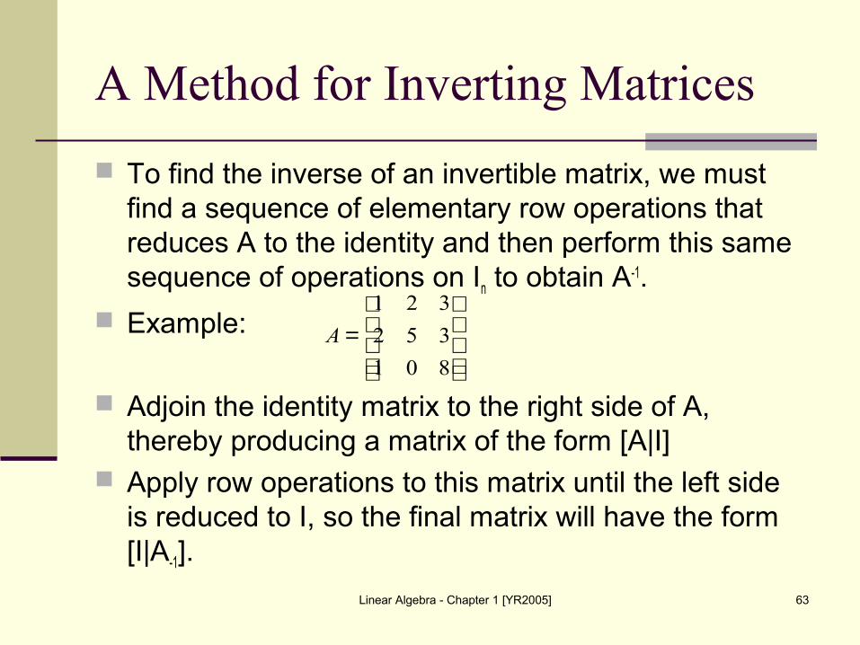
A Method for Inverting Matrices
To find the inverse of an invertible matrix, we must find a sequence of elementary row operations that reduces A to the identity and then perform this same sequence of operations on In to obtain A-1.
Example:
Adjoin the identity matrix to the right side of A, thereby producing a matrix of the form [A|I]
Apply row operations to this matrix until the left side is reduced to I, so the final matrix will have the form [I|A-1].
=
801
352
321
A

Linear Algebra - Chapter 1 [YR2005] 64
A Method for Inverting Matrices
Added –2 times the first row to the second and –1 times the first row to the third.
Added 2 times the second row to the third.
Multiplied the third row by –1.
Added 3 times the third row to the second and –3 times the third row to the first.
We added –2 times the second row to the first.
−−−−
−
−−−−
−
−−−
−
−−
−−
−−
−−
125
3513
91640
100
010
001
125
3513
3614
100
010
021
125
012
001
100
310
321
125
012
001
100
310
321
101
012
001
520
310
321
100
010
001
801
352
321

Linear Algebra - Chapter 1 [YR2005] 65
A Method for Inverting Matrices
Often it will not be known in advance whether a given matrix is invertible.
If elementary row operations are attempted on a matrix that is not invertible, then at some point in the computations a row of zeros will occur on the left side.
Example:
Added -2 times the first row to the second and
added the first row to the third.
Added the second row to the third.
−−=
521
142
461
A
−−−−
−−−
−−
111
012
001
000
980
461
101
012
001
980
980
461
100
010
001
521
142
461

Linear Algebra - Chapter 1 [YR2005] 66
Exercises
Consider the matrices
Find elementary matrices, E1, E2, E3, and E4, such that
a. E1A=B
b. E2B=A
c. E3A=C
d. E4C=A
−−−=
−−=
−−=
372
172
143
,
143
172
518
,
518
172
143
CBA
Linear Algebra - Chapter 1 [YR2005] 67
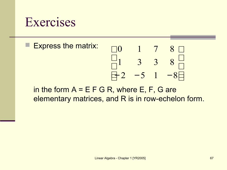
Exercises
Express the matrix:
in the form A = E F G R, where E, F, G are elementary matrices, and R is in row-echelon form.
−−− 8152
8331
8710

1.6 Further Results on
Systems of Equations and Invertibility

Linear Algebra - Chapter 1 [YR2005] 69
Linear Systems
Theorem:
Solving Linear Systems by Matrix Inversion:
If A is an invertible n x n matrix, then for each n x 1 matrix b, the system of equations Ax = b has exactly one solution, namely, x = A-1b.
Linear systems with a common coefficient matrix.Ax=b1, Ax=b2, Ax=b3, ..., Ax=bk
If A is invertible, then the solutions
x1=A-1b1, x2=A-1b2, x3=A-1b3, ..., xk=A-1bk
This can be efficiently done using Gauss-Jordan Elimination on [A|b1|b2|...|bk]

Linear Algebra - Chapter 1 [YR2005] 70
Linear Systems
Example: (a) (b)
The solution:
(a) x1=1, x2=0, x3=1
(b) x1=2, x2=1, x3=-1
98
5352
432
31
321
321
=+=++=++
xx
xxx
xxx
68
6352
132
31
321
321
−=+=++=++
xx
xxx
xxx
−
−
1
1
2
1
0
1
100
010
001
6
6
1
9
5
4
801
352
321

Linear Algebra - Chapter 1 [YR2005] 71
Properties of Invertible Matrices
Theorem: Let A be a square matrix.a) If B is a square matrix satisfying BA=I, then B=A-1.
b) If B is a square matrix satisfying AB=I, then B=A-1.
Theorem: Equivalent Statementsa) A is invertible
b) Ax=0 has only the trivial solutions
c) The reduced row-echelon form of A is In
d) A is expresssible as a product of elementary matrices
e) Ax=b is consistent for every n x 1 matrix b
f) Ax=b has exactly one solution for every n x 1 matrix b
Linear Algebra - Chapter 1 [YR2005] 72
Properties of Invertible Matrices
Theorem: Let A and B be square matrices of the same size. If AB is invertible, then A and B must also be invertible.
A fundamental problem.
Let A be a fixed m x n matrix. Find all m x 1 matrices b such that the system of equations Ax=b is consistent.

Linear Algebra - Chapter 1 [YR2005] 73
Exercises
Solve the system by inverting the coefficient matrix.
Find condition that b’s must satisfy for the system to be consistent.
6642
4973
744
032
=−−−−=+++=+++=−−−
zyxw
zyxw
zyxw
zyx
221
121
23
46
bxx
bxx
=−=−

1.7 Diagonal, Triangular,
and Symmetric Matrices

Linear Algebra - Chapter 1 [YR2005] 75
Diagonal Matrices
A square matrix in which all the entries off the main diagonal are zero. Example:
A diagonal matrix is invertible if and only if all of its diagonal entries are nonzero.
−
−
8000
0000
0040
0006
,
100
010
001
,50
02
=
nd
d
d
D
00
00
00
2
1
=−
nd
d
d
D
100
010
001
2
1
1
=
kn
k
k
k
d
d
d
D
00
00
00
2
1

Linear Algebra - Chapter 1 [YR2005] 76
Diagonal Matrices
Example:
−=
200
030
001
A
−=−
2
100
03
10
0011A
−=
200
030
0015A
−=−
321
24315
00
00
001
A
=
=
333322311
233222211
133122111
3
2
1
333231
232221
131211
343333323313
242232222212
141131121111
34333231
24232221
14131211
3
2
1
00
00
00
00
00
00
adadad
adadad
adadad
d
d
d
aaa
aaa
aaa
adadadad
adadadad
adadadad
aaaa
aaaa
aaaa
d
d
d

Linear Algebra - Chapter 1 [YR2005] 77
Triangular Matrices
Lower triangular = a square matrix in which all the entries above the main diagonal are zero.
Upper triangular = a square matrix in which all the entries under the main diagonal are zero.
Triangular = a matrix that is either upper triangular or lower triangular.
44
3433
242322
14131211
000
00
0
a
aa
aaa
aaaa
44434241
333231
2221
11
0
00
000
aaaa
aaa
aa
a

Linear Algebra - Chapter 1 [YR2005] 78
Triangular Matrices
Theorem: (basic properties of triangular matrices) The transpose of a lower triangular matrix is upper
triangular, and the transpose of an upper triangular matrix is lower triangular.
The product of lower triangular matrices is lower triangular, and the product of upper triangular matrices is upper triangular.
A triangular matrix is invertible if and only its diagonal entries are all nonzero.
The inverse of an invertible lower triangular matrix is lower triangular, and the inverse of an invertible upper triangular matrix is upper triangular.
Linear Algebra - Chapter 1 [YR2005] 79
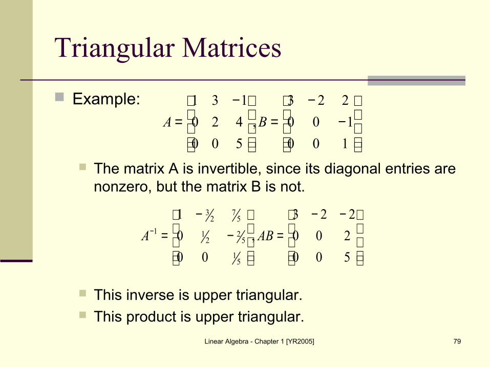
Triangular Matrices
Example:
The matrix A is invertible, since its diagonal entries are nonzero, but the matrix B is not.
This inverse is upper triangular. This product is upper triangular.
−
−=
−=
100
100
223
,
500
420
131
BA
−−=
−
−=−
500
200
223
,
00
0
1
51
52
21
57
23
1 ABA

Linear Algebra - Chapter 1 [YR2005] 80
Symmetric Matrices
A square matrix A is called symmetric if A = AT.
A matrix A = [aij] is symmetric if and only if aij=aji for all values of i and j.
−
−
−
4
3
2
1
000
000
000
000
,
705
034
541
,53
37
d
d
d
d
−
705
034
541

Linear Algebra - Chapter 1 [YR2005] 81
Symmetric Matrices
Theorem: If A and B are symmetric matrices with the same size, and if k is any scalar, then AT is symmetric A+B and A-B are symmetric kA is symmetric
Theorem: If A is an invertible matrix, then A-1 is
symmetric. If A is an invertible matrix, then AAT and ATA
are also invertible.
Linear Algebra - Chapter 1 [YR2005] 82
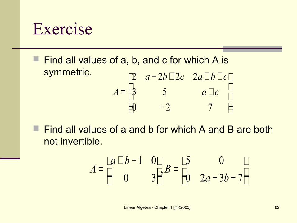
Exercise
Find all values of a, b, and c for which A is symmetric.
Find all values of a and b for which A and B are both not invertible.
−+
+++−=
720
53
2222
ca
cbacba
A
−−
=
−+=
7320
05,
30
01
baB
baA