Matlab software tools for model identification and data...

Model Identification and Data Analysis (Academic year 2017-2018)

Prof. Sergio Bittanti

Matlab software tools for model identification and data analysis

10/11/2017 Prof. Marcello Farina

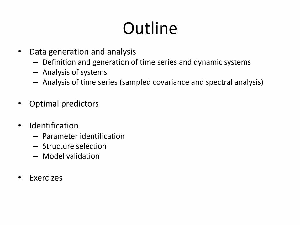
Outline • Data generation and analysis

– Definition and generation of time series and dynamic systems – Analysis of systems – Analysis of time series (sampled covariance and spectral analysis)

• Optimal predictors

• Identification

– Parameter identification – Structure selection – Model validation

• Exercizes

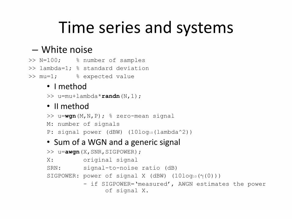
Time series and systems – White noise

>> N=100; % number of samples

>> lambda=1; % standard deviation

>> mu=1; % expected value

• I method >> u=mu+lambda*randn(N,1);

• II method >> u=wgn(M,N,P); % zero-mean signal

M: number of signals

P: signal power (dBW) (10log10(lambda^2))

• Sum of a WGN and a generic signal >> u=awgn(X,SNR,SIGPOWER);

X: original signal

SRN: signal-to-noise ratio (dB)

SIGPOWER: power of signal X (dBW) (10log10((0))) - if SIGPOWER=‘measured’, AWGN estimates the power

of signal X.

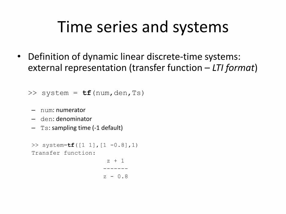
Time series and systems

• Definition of dynamic linear discrete-time systems: external representation (transfer function – LTI format)

>> system = tf(num,den,Ts)

– num: numerator

– den: denominator

– Ts: sampling time (-1 default)

>> system=tf([1 1],[1 -0.8],1)

Transfer function:

z + 1

-------

z - 0.8


• Step response of a LTI system >> T=[0:Ts:Tfinal];

>> [y,T]=step(system,Tfinal); % step response

>> step(system,Tfinal) % plot

• Response of a LTI system to a general input signal >> T=[0:Ts:Tfinal];

>> u1=sin(0.1*T); % e.g., sinusoidal input

>> u2=1+randn(T,1); % e.g., white gaussian noise

>> [y,T]=lsim(system,u1+u2,T);


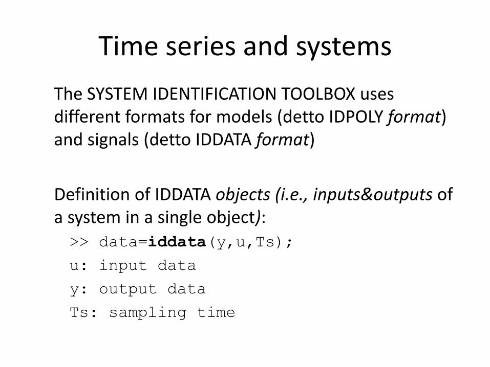
The SYSTEM IDENTIFICATION TOOLBOX uses different formats for models (detto IDPOLY format) and signals (detto IDDATA format)

Definition of IDDATA objects (i.e., inputs&outputs of a system in a single object): >> data=iddata(y,u,Ts);

u: input data

y: output data

Ts: sampling time

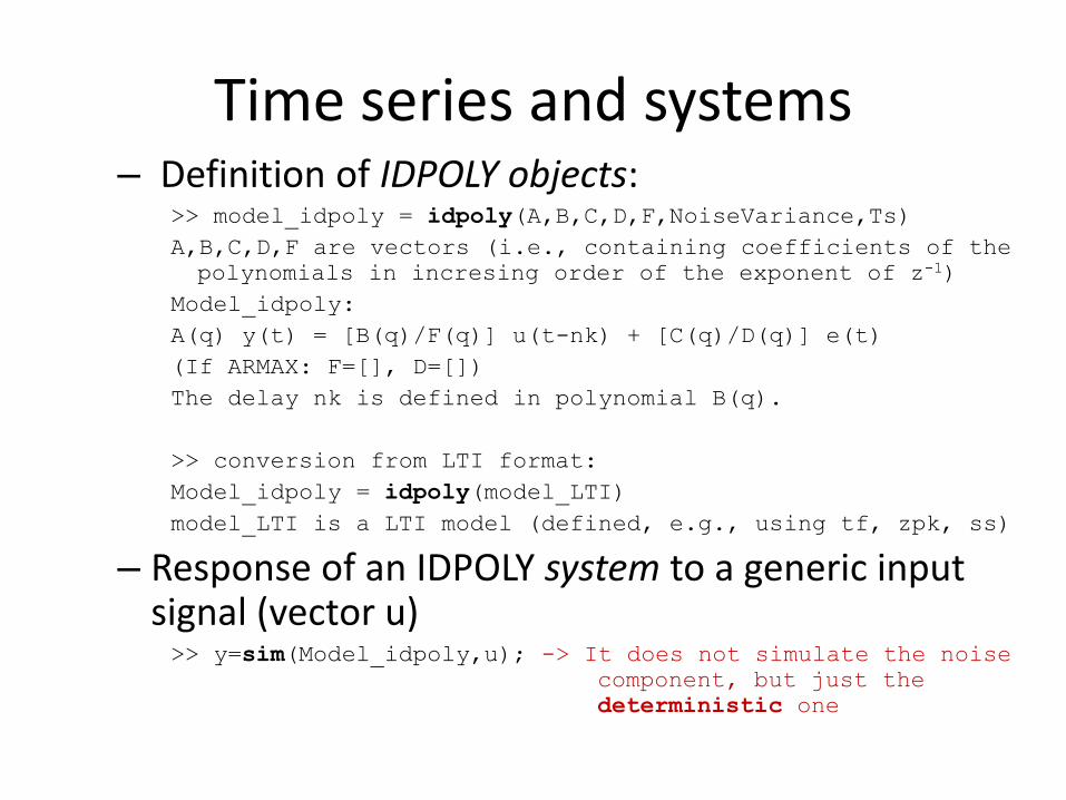
Time series and systems – Definition of IDPOLY objects:

>> model_idpoly = idpoly(A,B,C,D,F,NoiseVariance,Ts)

A,B,C,D,F are vectors (i.e., containing coefficients of the

polynomials in incresing order of the exponent of z-1)

Model_idpoly:

A(q) y(t) = [B(q)/F(q)] u(t-nk) + [C(q)/D(q)] e(t)

(If ARMAX: F=[], D=[])

The delay nk is defined in polynomial B(q).

>> conversion from LTI format:

Model_idpoly = idpoly(model_LTI)

model_LTI is a LTI model (defined, e.g., using tf, zpk, ss)

– Response of an IDPOLY system to a generic input signal (vector u)

>> y=sim(Model_idpoly,u); -> It does not simulate the noise

component, but just the

deterministic one


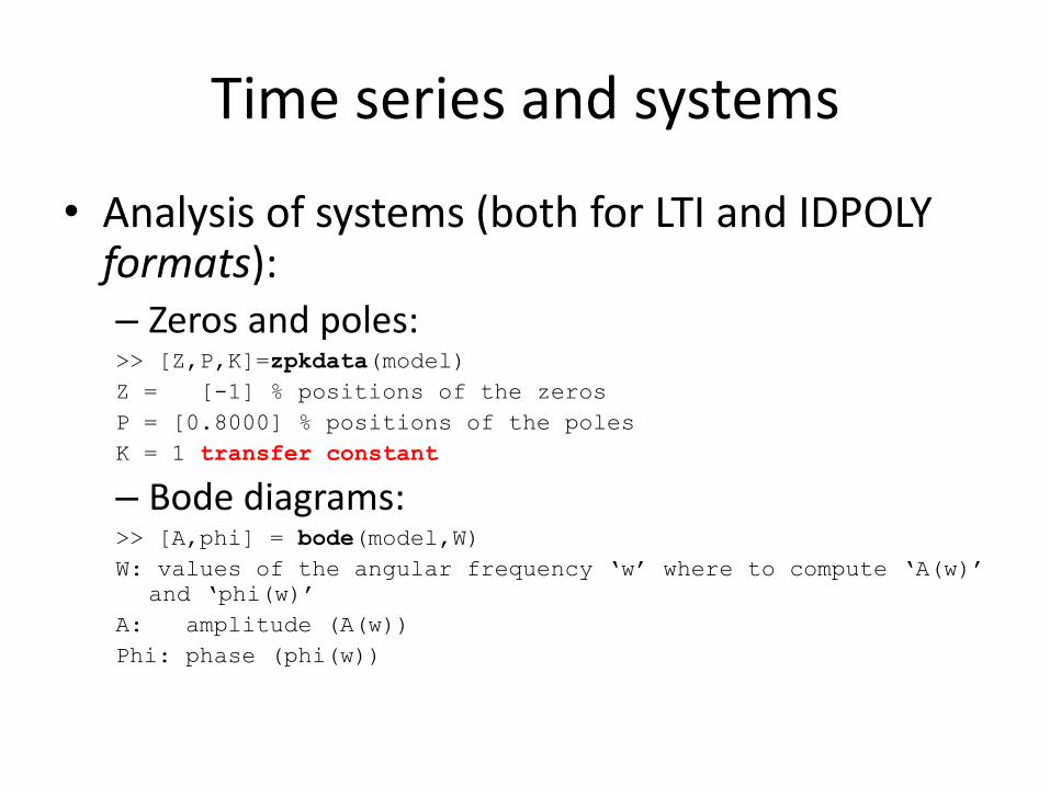
• Analysis of systems (both for LTI and IDPOLY formats): – Zeros and poles: >> [Z,P,K]=zpkdata(model)

Z = [-1] % positions of the zeros

P = [0.8000] % positions of the poles

K = 1 transfer constant

– Bode diagrams: >> [A,phi] = bode(model,W)

W: values of the angular frequency ‘w’ where to compute ‘A(w)’

and ‘phi(w)’

A: amplitude (A(w))

Phi: phase (phi(w))


– Bode diagrams:

>> [A,phi] = bode(model,[0.1 1])

A(:,:,1) =9.1179

A(:,:,2) =1.9931

phi(:,:,1) =-24.2456

phi(:,:,2) =-78.5036

>> bode(model)

>> % draws the Bode plots

(amplitude –dB- and phase)


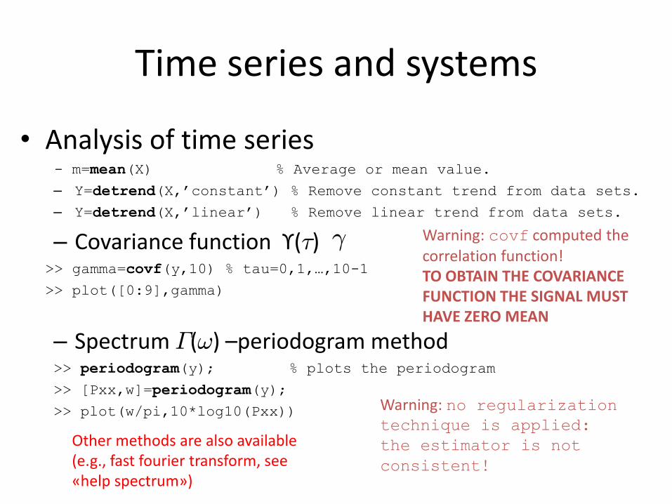
• Analysis of time series - m=mean(X) % Average or mean value.

– Y=detrend(X,’constant’) % Remove constant trend from data sets.

– Y=detrend(X,’linear’) % Remove linear trend from data sets.

– Covariance function ϒ(¿) >> gamma=covf(y,10) % tau=0,1,…,10-1

>> plot([0:9],gamma)

– Spectrum ¡(!) –periodogram method >> periodogram(y); % plots the periodogram

>> [Pxx,w]=periodogram(y);

>> plot(w/pi,10*log10(Pxx))

° Warning: covf computed the correlation function! TO OBTAIN THE COVARIANCE FUNCTION THE SIGNAL MUST HAVE ZERO MEAN

Warning: no regularization technique is applied:

the estimator is not

consistent!

Other methods are also available (e.g., fast fourier transform, see «help spectrum»)

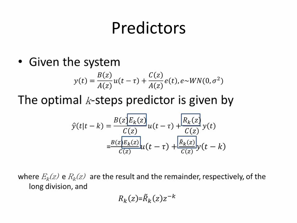
Predictors

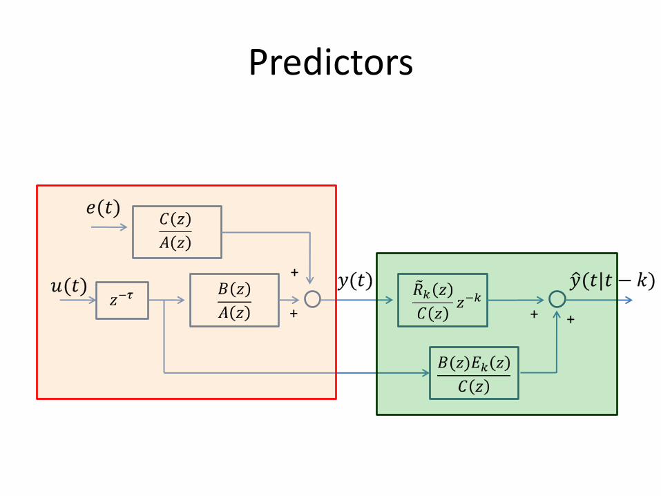
Predictors

+ +

+

+

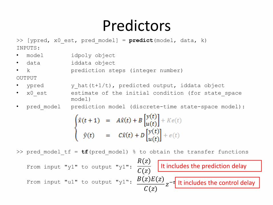
Predictors >> [ypred, x0_est, pred_model] = predict(model, data, k)

INPUTS:

• model idpoly object

• data iddata object

• k prediction steps (integer number)

OUTPUT

• ypred y_hat(t+1/t), predicted output, iddata object

• x0_est estimate of the initial condition (for state_space

model)

• pred_model prediction model (discrete-time state-space model):

>> pred_model_tf = tf(pred_model) % to obtain the transfer functions

From input "y1" to output "y1":

From input "u1" to output "y1“:

It includes the prediction delay

It includes the control delay

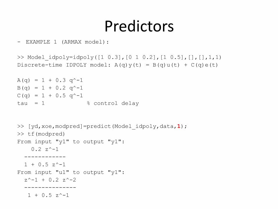
Predictors

- EXAMPLE 1 (ARMAX model):

>> Model_idpoly=idpoly([1 0.3],[0 1 0.2],[1 0.5],[],[],1,1)

Discrete-time IDPOLY model: A(q)y(t) = B(q)u(t) + C(q)e(t)

A(q) = 1 + 0.3 q^-1

B(q) = 1 + 0.2 q^-1

C(q) = 1 + 0.5 q^-1

tau = 1 % control delay

>> [yd,xoe,modpred]=predict(Model_idpoly,data,1);

>> tf(modpred)


0.2 z^-1

------------

1 + 0.5 z^-1

From input "u1" to output "y1":

z^-1 + 0.2 z^-2

---------------

1 + 0.5 z^-1

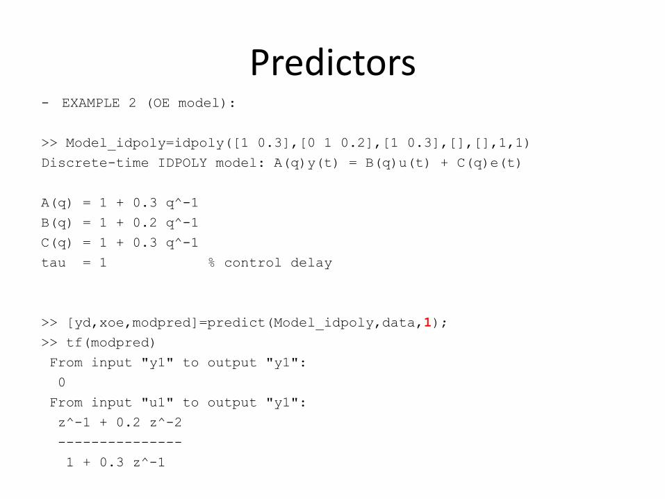
Predictors

- EXAMPLE 2 (OE model):

>> Model_idpoly=idpoly([1 0.3],[0 1 0.2],[1 0.3],[],[],1,1)


A(q) = 1 + 0.3 q^-1

B(q) = 1 + 0.2 q^-1

C(q) = 1 + 0.3 q^-1



>> tf(modpred)


0


z^-1 + 0.2 z^-2

---------------

1 + 0.3 z^-1

Predictors

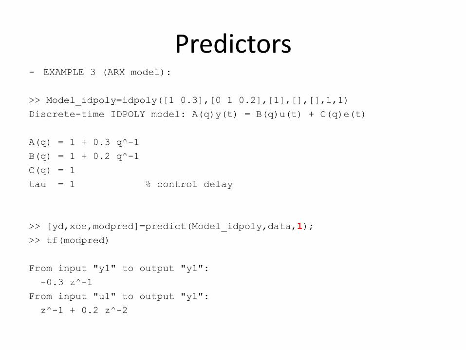
- EXAMPLE 3 (ARX model):

>> Model_idpoly=idpoly([1 0.3],[0 1 0.2],[1],[],[],1,1)


A(q) = 1 + 0.3 q^-1

B(q) = 1 + 0.2 q^-1

C(q) = 1



>> tf(modpred)


-0.3 z^-1


z^-1 + 0.2 z^-2

Predictors

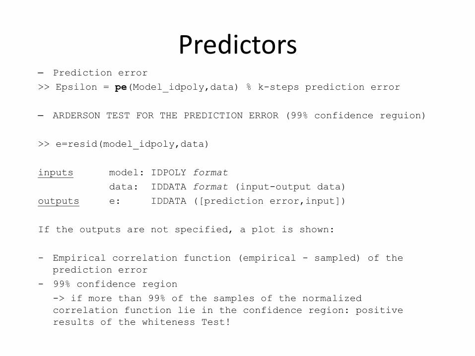
– Prediction error

>> Epsilon = pe(Model_idpoly,data) % k-steps prediction error

– ARDERSON TEST FOR THE PREDICTION ERROR (99% confidence reguion)

>> e=resid(model_idpoly,data)

inputs model: IDPOLY format

data: IDDATA format (input-output data)

outputs e: IDDATA ([prediction error,input])

If the outputs are not specified, a plot is shown:

- Empirical correlation function (empirical - sampled) of the

prediction error

- 99% confidence region

-> if more than 99% of the samples of the normalized

correlation function lie in the confidence region: positive

results of the whiteness Test!

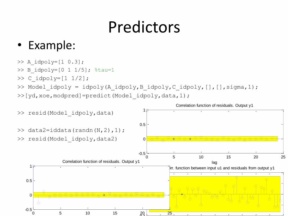
Predictors • Example:

>> A_idpoly=[1 0.3];

>> B_idpoly=[0 1 1/5]; %tau=1

>> C_idpoly=[1 1/2];

>> Model_idpoly = idpoly(A_idpoly,B_idpoly,C_idpoly,[],[],sigma,1);

>>[yd,xoe,modpred]=predict(Model_idpoly,data,1);

>> resid(Model_idpoly,data)

>> data2=iddata(randn(N,2),1);

>> resid(Model_idpoly,data2)

0 5 10 15 20 25-0.5

0

0.5

1Correlation function of residuals. Output y1

lag

-25 -20 -15 -10 -5 0 5 10 15 20 25-0.1

-0.05

0

0.05

0.1Cross corr. function between input u1 and residuals from output y1

lag

0 5 10 15 20 25-0.5

0

0.5

1Correlation function of residuals. Output y1

lag

-25 -20 -15 -10 -5 0 5 10 15 20 25-1

-0.5

0

0.5Cross corr. function between input u1 and residuals from output y1

lag

Identification >> systemIdentification % start the

MATLAB identification toolbox GUI

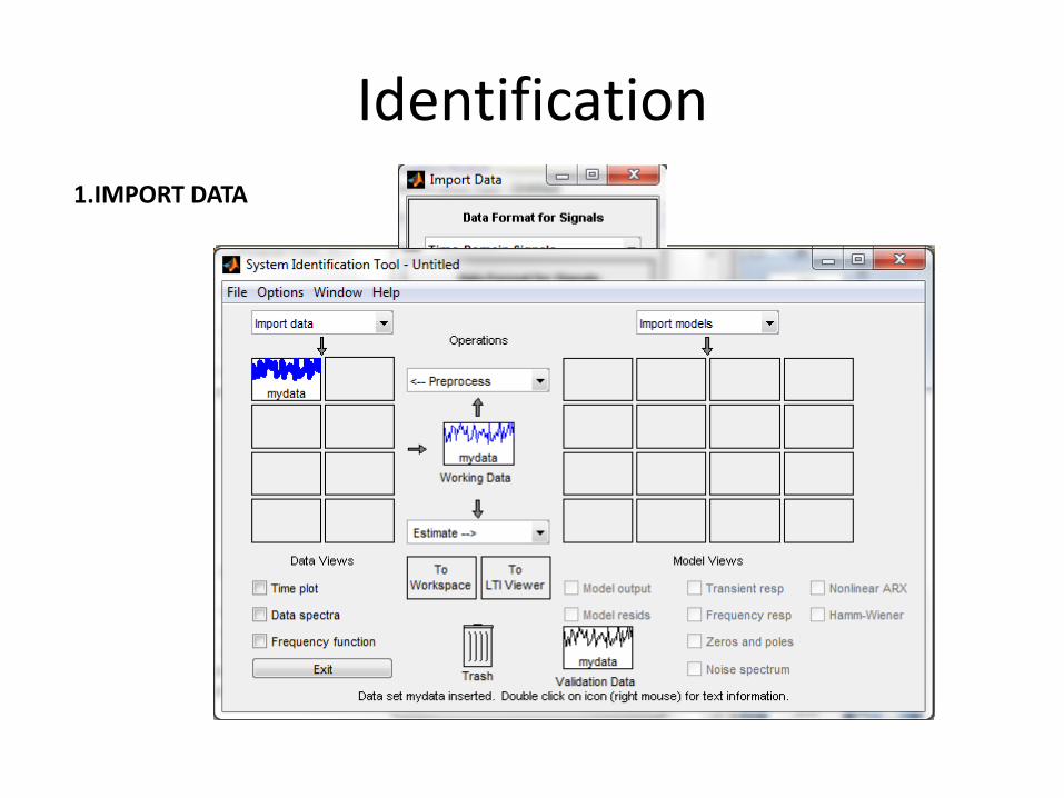
Identification

1.IMPORT DATA

Identification

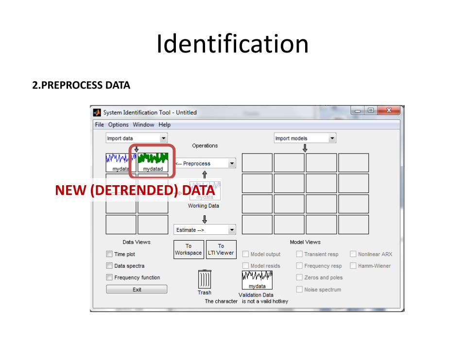
2.PREPROCESS DATA

NEW (DETRENDED) DATA

Identification

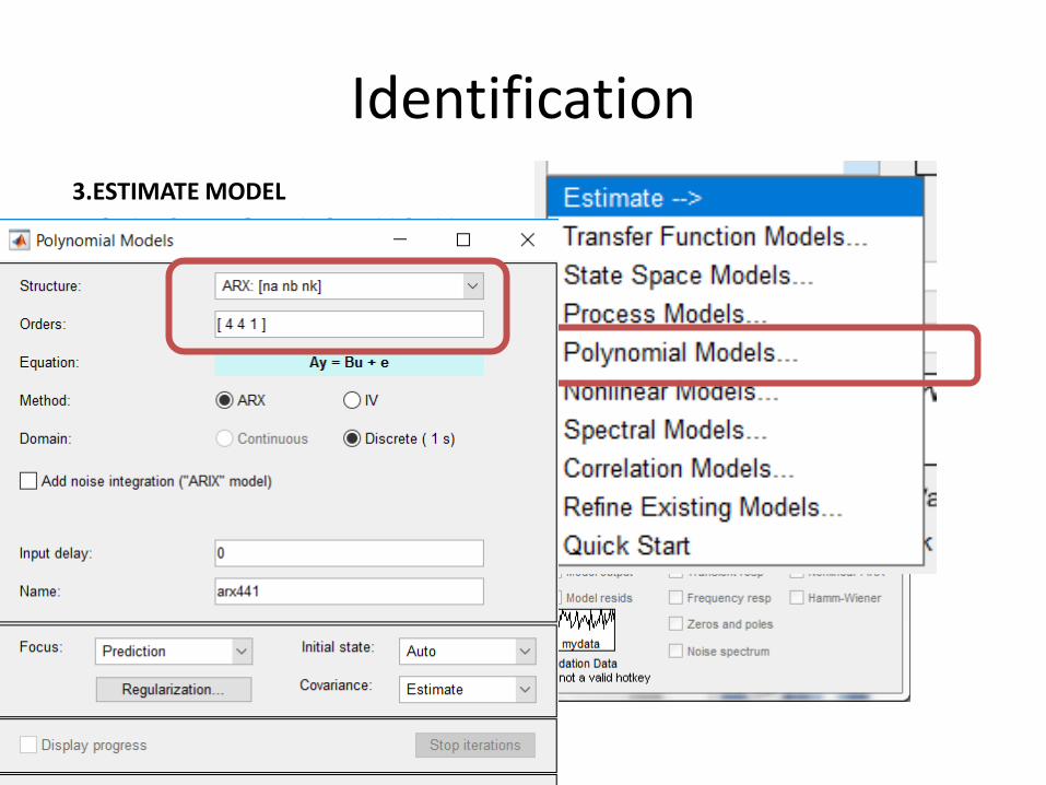
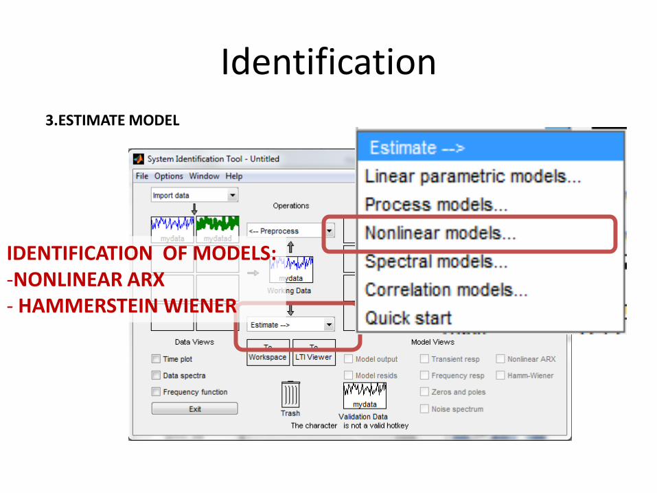
3.ESTIMATE MODEL

SELECT MODEL STRUCTURE

Identification

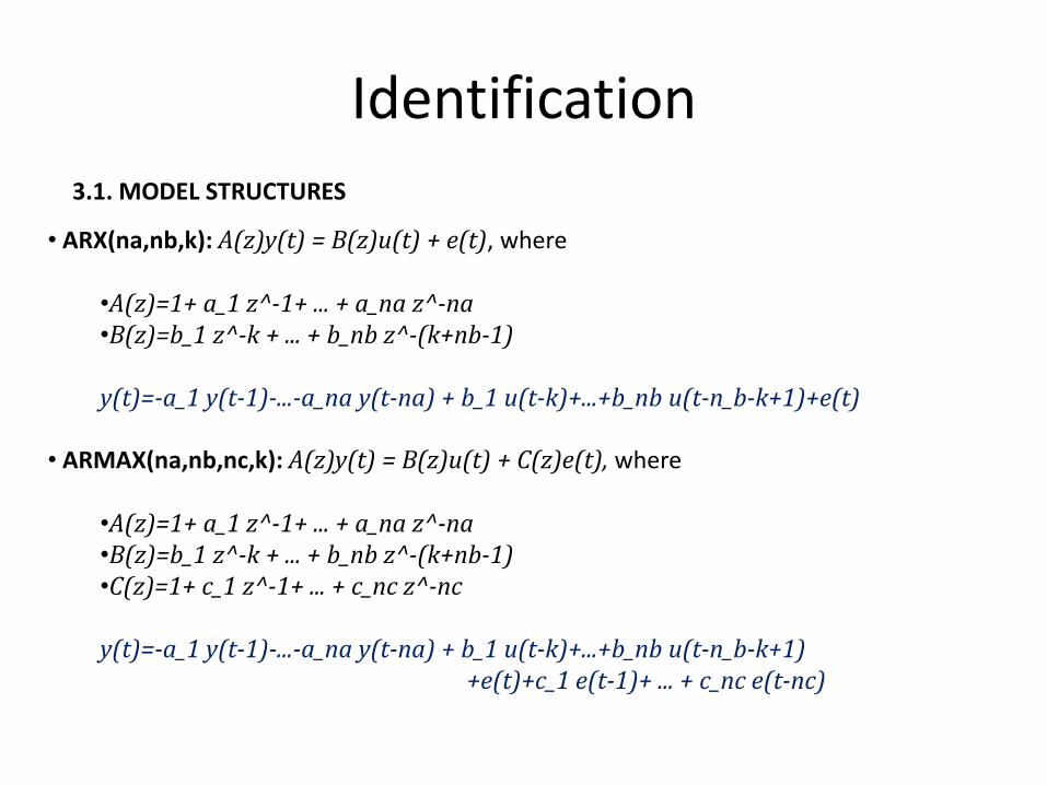
3.1. MODEL STRUCTURES

• ARX(na,nb,k): A(z)y(t) = B(z)u(t) + e(t), where

•A(z)=1+ a_1 z^-1+ ... + a_na z^-na •B(z)=b_1 z^-k + ... + b_nb z^-(k+nb-1) y(t)=-a_1 y(t-1)-...-a_na y(t-na) + b_1 u(t-k)+...+b_nb u(t-n_b-k+1)+e(t)

• ARMAX(na,nb,nc,k): A(z)y(t) = B(z)u(t) + C(z)e(t), where

•A(z)=1+ a_1 z^-1+ ... + a_na z^-na •B(z)=b_1 z^-k + ... + b_nb z^-(k+nb-1) •C(z)=1+ c_1 z^-1+ ... + c_nc z^-nc y(t)=-a_1 y(t-1)-...-a_na y(t-na) + b_1 u(t-k)+...+b_nb u(t-n_b-k+1) +e(t)+c_1 e(t-1)+ ... + c_nc e(t-nc)

Identification

3.1. MODEL STRUCTURES

• OE(nb,nf,k): y(t) = B(z)/F(z)u(t) + e(t), where

•B(z)=b_1 z^-k + ... + b_nb z^-(k+nb-1) •F(z)=1+ f_1 z^-1+ ... + f_nf z^-nf y(t)=-f_1 y(t-1)-...-f_na y(t-nf) + b_1 u(t-k)+...+b_nb u(t-n_b-k+1) +e(t)+f_1 e(t-1)+ ... + f_nf e(t-nf)

• BOX-JENKINS(nb,nc,nd,nf,k): y(t) = B(z)/F(z)u(t) + C(z)/D(z)e(t) • STATE-SPACE (n: order) [PEM or subspace identification]

x(t+1)=Ax(t)+Bu(t)+Ke(t) y(t)=Cx(t)+Du(t)+e(t)

Identification

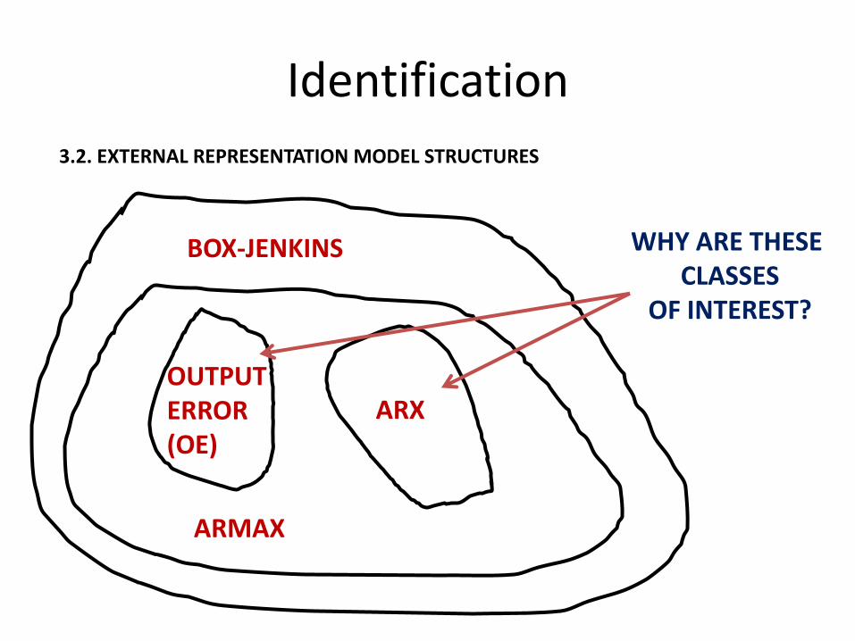
3.2. EXTERNAL REPRESENTATION MODEL STRUCTURES

BOX-JENKINS

ARMAX

OUTPUT ERROR (OE)

ARX

WHY ARE THESE CLASSES

OF INTEREST?

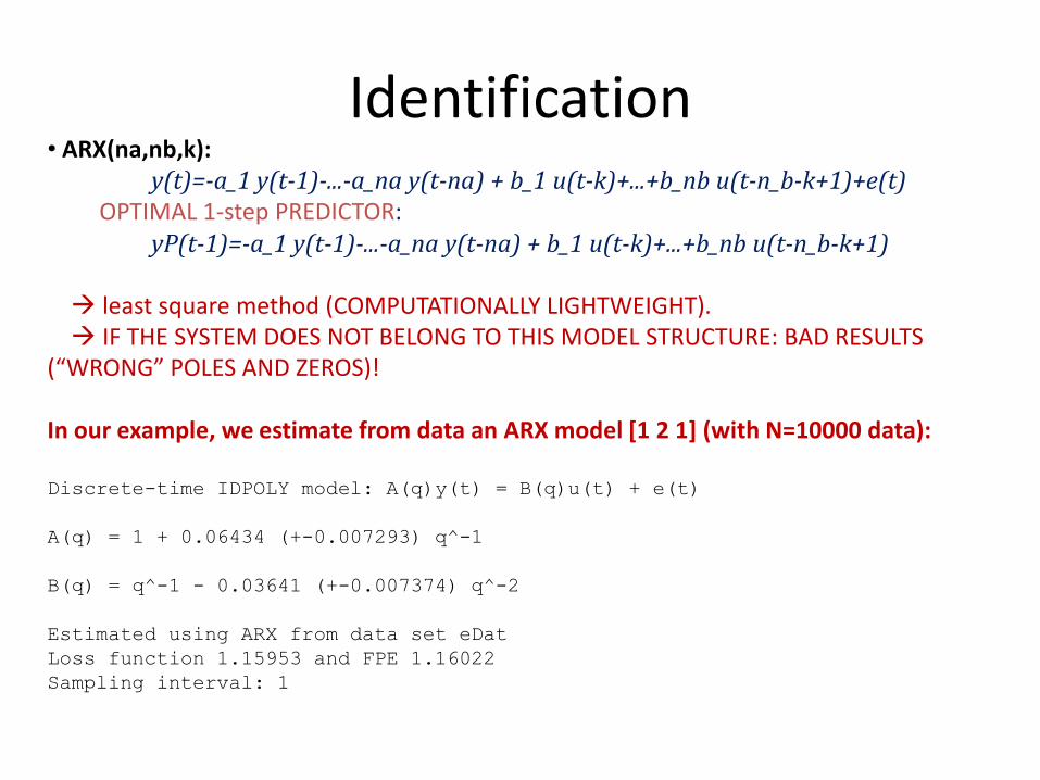
Identification • ARX(na,nb,k):

y(t)=-a_1 y(t-1)-...-a_na y(t-na) + b_1 u(t-k)+...+b_nb u(t-n_b-k+1)+e(t) OPTIMAL 1-step PREDICTOR: yP(t-1)=-a_1 y(t-1)-...-a_na y(t-na) + b_1 u(t-k)+...+b_nb u(t-n_b-k+1)

least square method (COMPUTATIONALLY LIGHTWEIGHT). IF THE SYSTEM DOES NOT BELONG TO THIS MODEL STRUCTURE: BAD RESULTS (“WRONG” POLES AND ZEROS)! In our example, we estimate from data an ARX model [1 2 1] (with N=10000 data): Discrete-time IDPOLY model: A(q)y(t) = B(q)u(t) + e(t)

A(q) = 1 + 0.06434 (+-0.007293) q^-1

B(q) = q^-1 - 0.03641 (+-0.007374) q^-2

Estimated using ARX from data set eDat

Loss function 1.15953 and FPE 1.16022

Sampling interval: 1

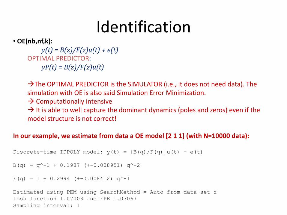
Identification • OE(nb,nf,k):

y(t) = B(z)/F(z)u(t) + e(t) OPTIMAL PREDICTOR: yP(t) = B(z)/F(z)u(t) The OPTIMAL PREDICTOR is the SIMULATOR (i.e., it does not need data). The simulation with OE is also said Simulation Error Minimization. Computationally intensive It is able to well capture the dominant dynamics (poles and zeros) even if the model structure is not correct!

In our example, we estimate from data a OE model [2 1 1] (with N=10000 data): Discrete-time IDPOLY model: y(t) = [B(q)/F(q)]u(t) + e(t)

B(q) = q^-1 + 0.1987 (+-0.008951) q^-2

F(q) = 1 + 0.2994 (+-0.008412) q^-1

Estimated using PEM using SearchMethod = Auto from data set z



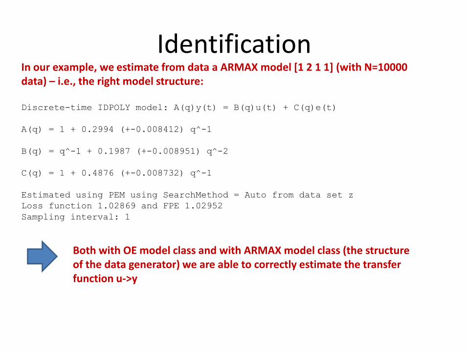
Identification In our example, we estimate from data a ARMAX model [1 2 1 1] (with N=10000 data) – i.e., the right model structure: Discrete-time IDPOLY model: A(q)y(t) = B(q)u(t) + C(q)e(t)

A(q) = 1 + 0.2994 (+-0.008412) q^-1

B(q) = q^-1 + 0.1987 (+-0.008951) q^-2

C(q) = 1 + 0.4876 (+-0.008732) q^-1

Estimated using PEM using SearchMethod = Auto from data set z



Both with OE model class and with ARMAX model class (the structure of the data generator) we are able to correctly estimate the transfer function u->y

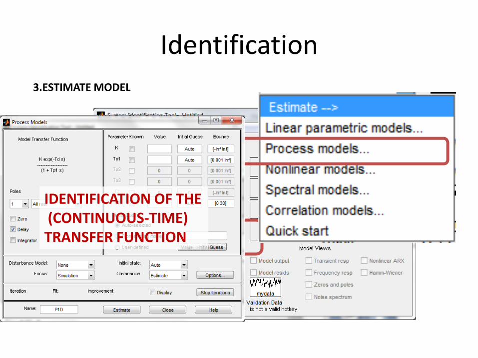
Identification

3.ESTIMATE MODEL

IDENTIFICATION OF THE (CONTINUOUS-TIME) TRANSFER FUNCTION

Identification

3.ESTIMATE MODEL

IDENTIFICATION OF MODELS: -NONLINEAR ARX - HAMMERSTEIN WIENER

Identification

4.Compare and validate models

For further details, see

http://it.mathworks.com/products/sysid/

Identification

Identification Other related Matlab functions (2 Identification toolbox)

• Parametric model estimation – ar - AR-models of signals using various approaches.

– armax - Prediction error estimate of an ARMAX model.

– arx - LS-estimate of ARX-models.

– bj - Prediction error estimate of a Box-Jenkins model.

– ivar - IV-estimates for the AR-part of a scalar time series (with instrumental variable method).

– iv4 - Approximately optimal IV-estimates for ARX-models.

– n4sid - State-space model estimation using a sub-space method.

– nlarx - Prediction error estimate of a nonlinear ARX model.

– nlhw - Prediction error estimate of a Hammerstein-Wiener model.

– oe - Prediction error estimate of an output-error model.

– pem - Prediction error estimate of a general model.

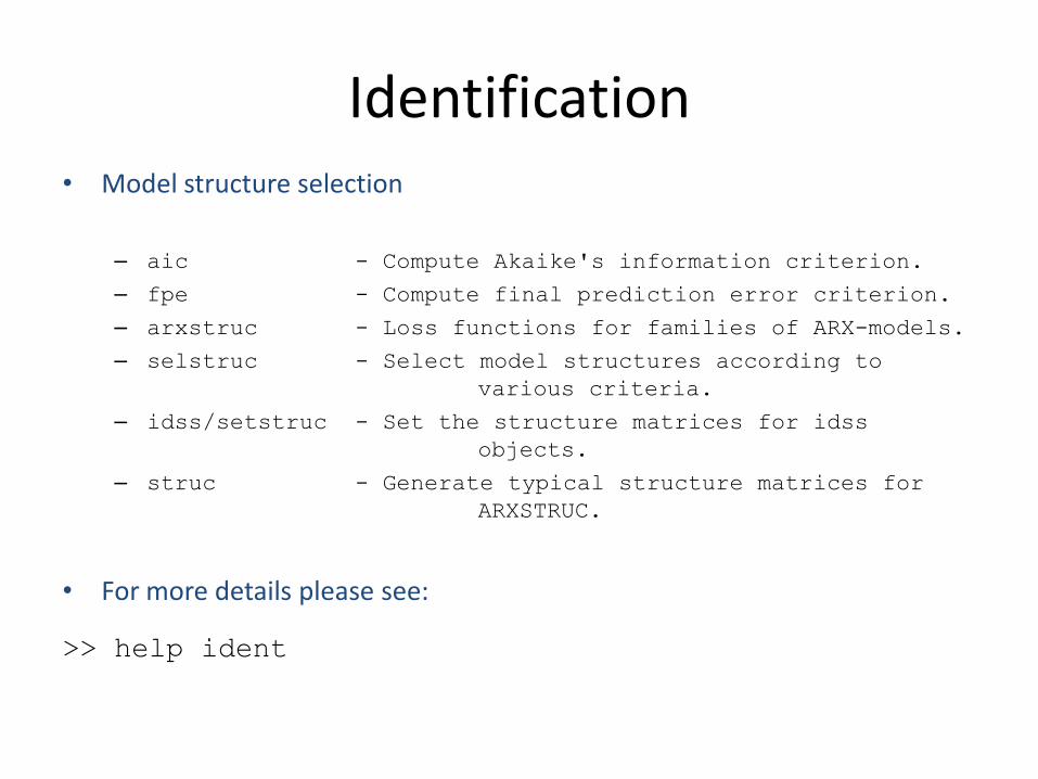
Identification • Model structure selection

– aic - Compute Akaike's information criterion.

– fpe - Compute final prediction error criterion.

– arxstruc - Loss functions for families of ARX-models.

– selstruc - Select model structures according to

various criteria.

– idss/setstruc - Set the structure matrices for idss

objects.

– struc - Generate typical structure matrices for

ARXSTRUC.

• For more details please see:

>> help ident

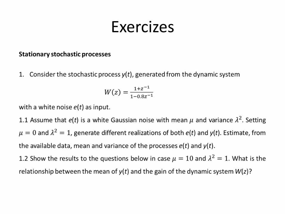
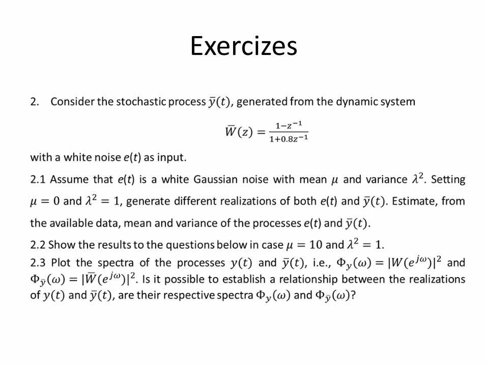
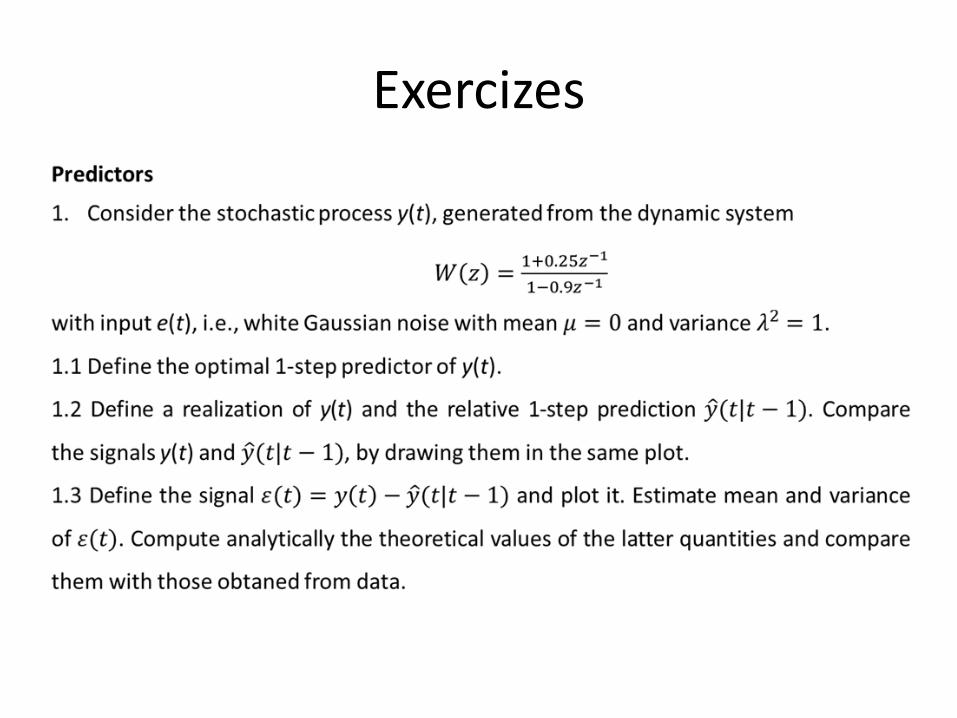
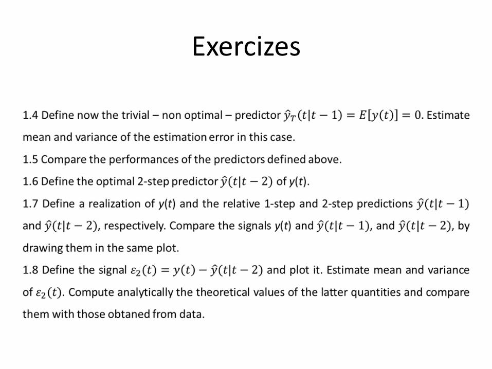
Exercizes

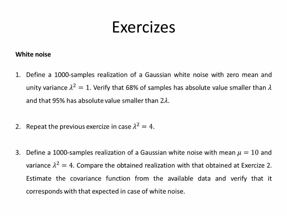
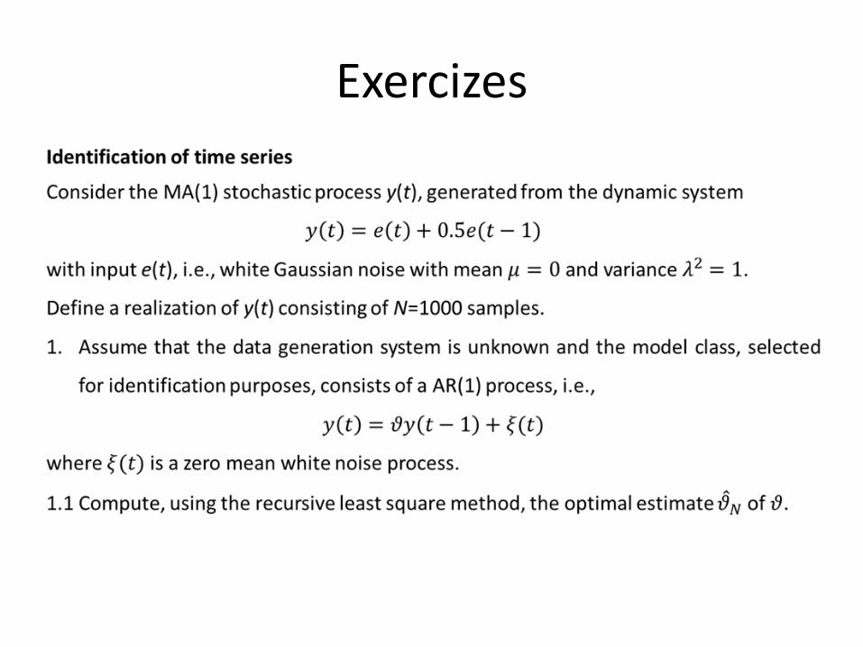
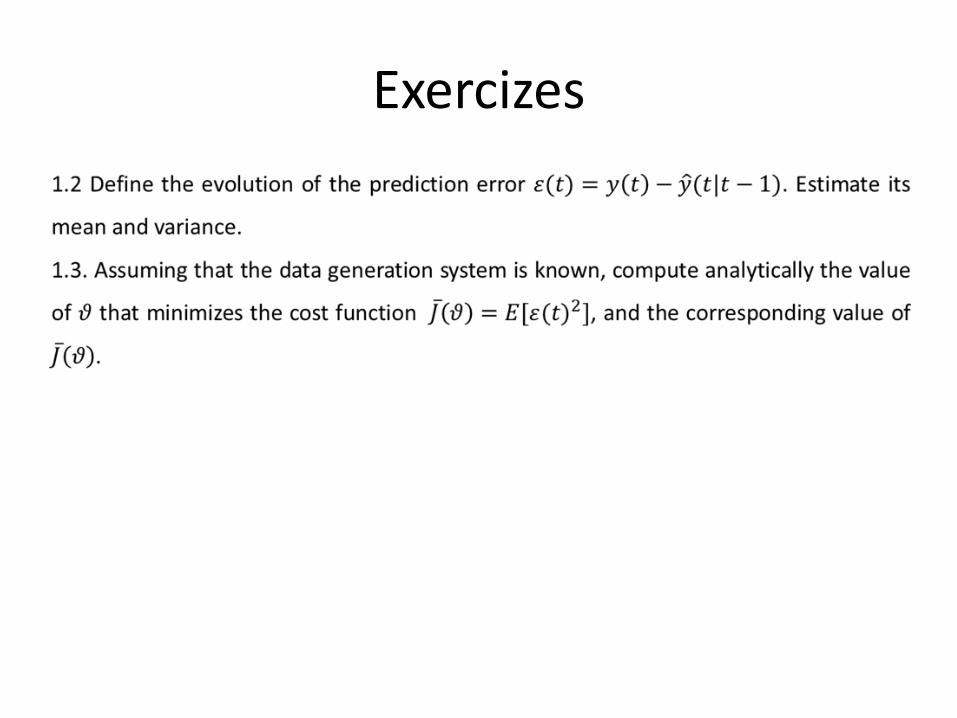
Exercizes

Model Identification Consider the ARMAX system y(t)=0.1 y(t-1)+2u(t-1)-0.8 u(t-2)+e(t)+0.3e(t-1) Where e(t) is a white noise with zero mean and unitary variance. 1. Generate a 1000-samples realization of the output signal y(t), when the input

u(t) is a persistently exciting signal (e.g., a white noise), and where y(0)=0;. 2. Identify, using the identification toolbox:

1. an ARX(1,1,1) model 2. an ARX(1,2,1) model 3. an ARMAX(1,2,2,1) model 4. an ARMAX(1,1,2,1) model 5. an OE(2,1,1) model

3. Compare and analyze the results (possibly add validation data to validate the results).

Exercizes

Matlab software tools for model identification and data...

Documents

Transcript of Matlab software tools for model identification and data...