Matlab Simulink Model of a Braked Rail Vehicle and Its ...

Grazyna BarnaRail Vehicles Institute ”TABOR”

Poland

1. Introduction

When a braking force applied to the axle sets of a rail vehicle exceeds a critical value, whichdepends on the wheel-rail adherence, the wheels start to slide. If no corrective action is taken,in a very short time the wheels can be locked. Locking of the wheels or their excessive slidecan result in increased braking distance and damage to the wheel rims (flat spots, also called”flats”). Wheel flats are sources of vibration and noise, they lower riding quality of a vehicleas well as passenger comfort, but first and foremost increasing of the braking distance directlyimpairs safety of the train staff and passengers and also of people nearby. In order to preventexcessive wheel slide and wheel lock, rail vehicles are equipped with Wheel Slide Protection(WSP) systems.

From the point of view of a WSP controller, the rail vehicle is a strongly non-linear andnon-stationary plant. From the other hand there exist intuitive expert knowledge concerningthe way the slide should be controlled. For these two reasons fuzzy logic controllers (FLC) arewidely used in WSP systems (Caldara et al. (1996), Barna (2009)).

One of the basic problems concerning FLCs is lack of formal methods of design. Designing therule bases of the fuzzy controllers is usually performed using a trial-and-error method, whichin turn requires performing numerous tests of the controlled plant. When a controlled plant isa rail vehicle, possibilities of performing such tests are very limited due to high costs of testsand danger of damaging the wheels. A commonly used solution to this problem is employinga simulator of a braked rail vehicle, which can be used for preliminary design, optimizationand tuning of the controllers. Tests on a real object are performed at the last stage of the designprocess in order to verify the designed controller.

The purpose of this chapter is to present the Matlab Simulink� model of a braked rail vehicleand its many applications, which comprise both designing and testing of the WSP systems. Inthe next two introductory sections the slide phenomenon as well as the structure and principleof operation of WSP systems are described in order to provide the readers who are not familiarwith the WSP devices with some useful information which would facilitate reading of thischapter.

2. Slide during braking of a rail vehicle

During braking of a rail vehicle, a braking torque generated by a rail vehicle braking systemis applied to the axle sets. When a value of this torque exceeds a boundary value, which

Matlab Simulink® Model of

a Braked Rail Vehicle and Its Applications

9

www.intechopen.com

2 Will-be-set-by-IN-TECH

depends on the instantaneous value of wheel-rail adherence, than the circumferential speedof the wheels starts to decrease (which is called sliding). If no corrective action is taken, in avery short time the wheels can be locked.

Locking of the wheels of a rail vehicle, as well as an excessive wheel slide have severalnegative consequences, out of which two are critical. First and foremost, due to decreasingof the adhesion coefficient, the braking force remains constant at a small value, which makesimpossible effective braking of a vehicle and results in significant increasing of the brakingdistance. As an example, the braking distance of a 150A passenger car braked at 120 km/hamounts, according to both field and simulation tests approximately 480 m, while at brakingwith all the wheels locked at the beginning of braking it can be increased even up to 800 m.Increasing of the braking distance impairs the safety of passengers, train staff and peoplein proximity. Secondly, when locked wheels slide along the rails, flat spots (called "flats")can be produced on wheel treads. The depth of a wheel flat can amount up to severalmillimeters (Pawełczyk (2008)), especially in case of a prolonged slide. In Fig. 1 and Fig. 2photographs of wheel flats of a passenger car wheels are shown.

Fig. 1. Flat spot on a wheel tread 1

Fig. 2. Flat spot on a wheel tread 2

Increase of the temperature of the sliding wheel and rapid cooling of the outer wheellayer, caused by regaining speed after the wheel slide has ceased, may result in formingof martensite around the flat spot. Martensite is a form of steel, firm, but fragile, which is

190 Technology and Engineering Applications of Simulink

www.intechopen.com

Matlab Simulink� Model of a Braked Rail Vehicle and its Applications 3

subjected to cracks and crumbling. It develops first of all at the surface, and then propagatingfar into the wheel material. It results in developing the loss of the material of the wheeltreads (Jergéus (1998); Kwasnikowski & Firlik (2006)).

Damage to the wheel treads may be caused not only by wheel lock, but also by excessivedifference (above 30 km/h) between vehicle velocity and circumferential velocity of a wheel.

Vibrations also lower the comfort of the passengers and the trains staff, negatively influencingtheir mood and ability to work after the journey, and also their health. In Fig. 3 simulationcharacteristics are shown for both a vehicle with round wheels and a vehicle with one flatspot on one wheel, at speed 140 km/h. The influence of a flat spot is seen the most clearly forfrequency of app. 13,5 Hz. Lowering of comfort, defined as increasing of the effective valueof vertical acceleration in the middle of the body amounts in this particular case to app. 30 %,and it depends on the vehicle velocity (Ofierzynski (2008)).

The concern about wheel slide has increased, as rail vehicles began running at higher speeds,because not only braking torque which is necessary to brake a vehicle needs to be bigger,which increases the probability of the wheel slide, but also consequences of such event aremore serious when it occurs at high vehicle velocities.

To prevent the described above situations, rail vehicles are equipped with Wheel SlideProtection (WSP) devices, which detect slide of the vehicle wheels and adequately controlthe braking torque, not only preventing wheels from being locked, but also increasing theadhesion coefficient value, thus making the braking distance as short as possible.

Because a safety critical system is a system the failure of which can result in severeconsequences, e.g. death or injury of people, or significant damages to property orenvironment, thus it is evident that a WSP device is a safety critical system (Barna & Kaluba(2009)). Standard CEN (2009) and leaflet UIC (2005) contain specification of requirements forboth structure and functions of WSP devices.

Fig. 3. Swing and frequency characteristics of vertical acceleration in the middle of thepassenger car body, respectively without and with a wheel flat (Ofierzynski (2008))

3. Wheel Slide Protection systems

A WSP system consists of the following elements: wheel speed sensors, controller and dumpvalves. The block diagram of a WSP system for a two-axle bogie with block brake is shown inFig. 4 ( Barna (2009), UIC (2005), CEN (2009)).

A WSP controller on the basis on signals from speed sensors of all wheel-sets, performscalculation of circumferential wheel velocities and determines circumferential wheel

191Matlab Simulink® Model of a Braked Rail Vehicle and Its Applications

www.intechopen.com


Fig. 4. Block diagram of a WSP system: DV1, DV2 - dump valves, V1, V2 - speedmeasurement signals, EV1, EV2, BV1, BV2 - dump valve control signals

accelerations and wheel slides, performs estimation of vehicle velocity (called the referencevelocity), and then, on the basis of the obtained values appropriately controls the dumpvalves, in order to adjust the braking torque to the instantaneous adhesion conditions (Barna(2010a)). When a slide is detected, the braking torque should be adequately decreased byproper control of the dump valves; after recovery of adhesion the torque should be increasedin order to provide effective braking of the vehicle.

Speed sensors make possible measuring the angular speeds of the wheels – they generatesquare-wave signals from which circumferential wheel speeds can be calculated, and whichare main input signals for the WSP controller.

The WSP actuators are dump valves, mounted as close as possible to the brake cylinders.The valves can adopt one of the three states, which makes possible increasing, decreasing ormaintaining the pressure value in the brake cylinders:

• filling of the cylinders (F)

• venting of the cylinders (V)

• cutting-off the air supply without venting (H).

Both filling and venting of the dump valves can be performed in one of the two followingways (Boiteux (1999)):

• continuous: applying either F or V state

• graduated: increasing or decreasing of the pressure are realized by applying repeatedsequences of respectively F and H or V and H states.

In Barna (2009) seven levels of pressure change have been proposed, designated P1, P2, P3,U1, U2, U3, H. The levels are obtained by cyclical applying sequences of the three mentionedabove states of the valves P3: P, P2: P H, P1: P H: H, U1: U H H, U2: U H, U3: U. Each of thestates is applied for a defined period of time, e.g. 100 ms.


www.intechopen.com


4. Characteristics of the WSP controllers

Wheel Slide Protection (WSP) devices control braking torque, not only preventing wheelsfrom being locked, but also increasing the adhesion coefficient value, making the brakingdistance as short as possible. Thus the main task of WSP systems is ”to make the best use ofavailable adhesion for all intended-operating conditions by a controlled reduction and restoration ofthe brake force to prevent axle sets from locking and uncontrolled sliding due to low adhesion” (CEN(2009)).

The main difficulties concerning the control algorithm resulting from the characteristics of abraked rail vehicle as a controlled plant are listed below, the first two out of which are themost crucial:

• instantaneous value of the coefficient of adhesion between wheel and rail ψ cannot bemeasured

• translation vehicle speed vT is usually not measured due to costs

• controlled plant is highly non-linear

– characteristics ψ = f (s) is non-linear (see Fig. 13)

– characteristics Mb = f (pc) is characterized by hysteresis

– dump valves behavior is non-linear

• controlled plant is non-stationary — parameters of characteristics ψ = f (s) change in away which is possible to comprehend in stochastic manner only

• direct control of a braking torque is not possible; actuators control the pressure values inthe brake cylinders

• controlling of the brake cylinder pressures is performed indirectly and discretely

• instantaneous values of the cylinder pressures are not known.

The task of a WSP controller is to achieve the highest possible at the current adhesionconditions adhesion forces (forces transferred to the wheels of the axle sets), which isequivalent with achieving the shortest possible braking distance. This goal is achieved, asmentioned in Section 3 by proper control of the dump valves of each axle set.

In Fig. 5 a trajectory ψ = f (s) for an optimally working controller has been shown,superimposed on a generalized adhesion versus slide curve. A WSP device equipped withsuch a controller, called in Boiteux (1999) a Second Generation WSP, realizes control in theneighbourhood of the point B of an adhesion curve and maintains a value of a relative slide sclose to its optimum value sB (see subsection 5.2.4).

A control system such as described above is called an extremum regulation system. The taskof the extremum regulation system is maintaining a controlled signal as close as possible tothe extremum value, which changes depending on disturbance signals (Kaczorek (1977)). Inthe case of a braked rail vehicle and a WSP controller this extremum value should be theinstantaneous value of adhesion coefficient between wheel and rail ψ.

In Fig. 6 an overall block diagram of a WSP control system is shown, which is a base forpractically realized control algorithms of WSP controllers.

A braked rail vehicle as a control plant is strongly non-linear and non-stationary,therefore the WSP controllers are usually designed using Fuzzy Logic and Expert


www.intechopen.com


s

ψ

α

B

A

1

Fig. 5. The principle of operation of an optimal Wheel Slide Protection (Boiteux (1999))

Δ

σ(k)

∆v(k)

∆2v(k)

Δ

V O(k),V L(k) ∆pc(k) v(k)

ControllerDumpvalves

Railvehicle

Speedsensors

Determiningthe referencespeed

+

−

vref (k)

σ(k)

Fig. 6. Practical block diagram of WSP control system (Barna (2009))

Knowledge techniques (Caldara et al. (1996); Cheok & Shiomi (2000); Mauer (1995); Sanz &Pérez-Rodríguez (1997); Will & Zak (2000)).

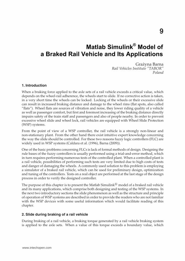
The WSP control system using Fuzzy Logic controllers implemented in Matlab Simulink� is

shown in Fig. 7. The control system is realized as Triggered Subsystem Simulink� block,triggered every 100 ms, which corresponds to a real controller program cycle time. The

controller blocks for every axle are implemented with Fuzzy Logic Controller Simulink�

blocks. The inputs for each FLC block are absolute axle slide σ [km/h] and axle acceleration a,which are calculated on the basis of the measured wheel circumferential velocities and vehiclereference velocity vref , as shown in Fig. 6. The measured wheel circumferential velocities are


www.intechopen.com


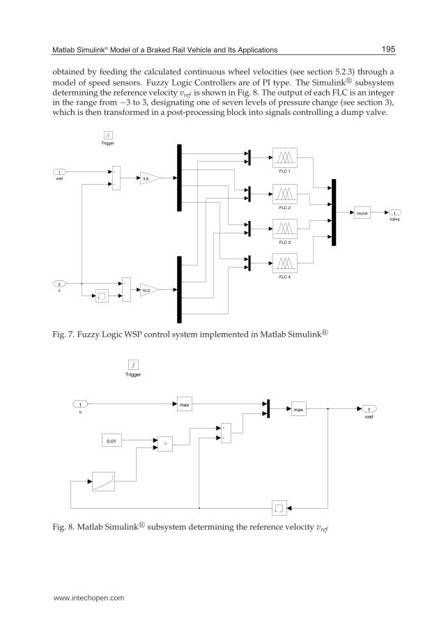
obtained by feeding the calculated continuous wheel velocities (see section 5.2.3) through a

model of speed sensors. Fuzzy Logic Controllers are of PI type. The Simulink� subsystemdetermining the reference velocity vref is shown in Fig. 8. The output of each FLC is an integerin the range from −3 to 3, designating one of seven levels of pressure change (see section 3),which is then transformed in a post-processing block into signals controlling a dump valve.

Valve

1round

3.6

10.0

FLC 4

FLC 3

FLC 2

FLC 1

Trigger

v

2

vref

1

Fig. 7. Fuzzy Logic WSP control system implemented in Matlab Simulink�

vref

1

0.01

maxmax

Trigger

v

1

Fig. 8. Matlab Simulink� subsystem determining the reference velocity vref


www.intechopen.com


5. Simulator of a braked rail vehicle

5.1 Introduction

Designing and testing of the FLC WSP controllers demands performing numerousexperiments. Performing tests using a real rail vehicle is not feasible, because of high costsand possibility of damaging the object, therefore for designing and testing WSP controllers atest stand is indispensable. One of the most important elements of the test stand is a simulatorof a braked rail vehicle.

The mathematical model of a braked rail vehicle, simulation model and various versions of asimulation stand are presented in this subsection.

5.2 Mathematical model of a braked rail vehicle

5.2.1 Introduction

The basis for a rail vehicle simulator is a mathematical model of a braked rail vehicle,taking into consideration the basic phenomena occurring during sliding and omitting thephenomena that are of no or slight significance.

The model has the following parameters:

• parameters describing properties of the vehicle (e.g. mass, number of axles, inertia of theaxle sets)

• vehicle velocity in the moment of commencement of braking

• intensiveness of braking defined as the maximum pressure in the brake cylinders.

The inputs to the model are:

• state of dump valves generated by the WSP controller

• state of the rail (adhesion coefficient).

The purpose of the model is performing the simulations of braking of a rail vehicle at reducedadhesion. Therefore all the basic phenomena influencing the wheel speeds during brakingmust be modeled as faithfully as feasible. A special attention must be put to all the mainnon-linear subsystems of the system. The most important example is the wheel-rail adhesioncoefficient.

Some simplifying assumptions have been adopted, which simplify the model, while do notsignificantly alter its functionality. One of these assumptions is considering the vehicle as arigid body with the agglomerated mass.

The model consists of the following subsystems:

• model of a braking system

• model of a rotational motion of a wheel-set

• model of the adhesion curve

• model of a translation vehicle motion.

The subsystems of the model are described in the subsequent subsections.


www.intechopen.com


5.2.2 Model of a braking system

The model of the braking system describes the relation between pressure in the brakecylinders of the axle set and its braking torque.

This model can be divided into the following three subsystems:

• model of the pneumatic system and the dump valves

• model of the lever system

• model of the friction elements.

5.2.2.1 Model of the pneumatic system and the dump valves

The pressure at the input of a dump valve can be described with the followingequation (Kaluba (1999)):

pc in = pcmax

(

1 − e−0.75t)

. (1)

The dump valves are a part of delivery of the WSP system. However, from the modelingpoint of view, because they are integrated into the pneumatic system of the vehicle, they areconsidered as part of this system.

The dump valve has been modeled as the inertia element of adjustable time constantindependently for filling TF and venting TV .

The pressure in the brake cylinders supplied by the valve are given with one of the followingequations:

for filling

pc = p0 + (pc in − p0)

(

1 − e− t−tz

TF

)

, (2)

for venting

pc = p0e−

t−t0TV , (3)

and for holdingpc = p0. (4)

5.2.2.2 Model of the lever system

The relation between the pressure of the friction linings of the brake blocks onto the wheeltreads of the brake disks, which is exerted by the piston of the brake cylinder and the pressurein the brake cylinder is highly non-linear and is characterized by hysteresis, resulting fromfriction in the brake cylinder and in the joints of the clamp mechanism (Knorr (2002); Tao &Kokotovic (1996)). This relation is shown in Fig. (9). The two rays limiting the area are givenwith:

Nk1 = (pc Ak − Ff )ηsηrip, (5)

Nk2 = (pc Ak − Ff )(2 − ηsηr)ip. (6)


www.intechopen.com


holding

holding

venting

filling

pc

Nk

pc1pc2pFf

Nk1Nk2

Fig. 9. Relation between the air pressure in brake cylinders and the brake blocks pressure

5.2.2.3 Model of the friction elements

Because some vehicles are equipped with disk brakes and some with block brakes, models ofboth types of brakes have been prepared.

For both types of the brakes the braking torque is given with:

Mb = Nkμrb, (7)

where rh is the braking radius.

For the block brake, the braking radius rh is equal to the wheel radius r, for the disk brake itis equal to the radius of the brake disk rd.

The friction coefficient between the friction linings of the brake blocks and the wheel tread orthe brake disk μ depends in a non-linear way on many factors, first of all on wheel velocityand pressure of the disk block.

A simplified value of the friction coefficient μ for a block brake is given with the empiricalequation. In this model the equation given in Sachs (1973) has been adopted:

μ = 0, 163

√

40, 25

v3

√

2, 461

px, (8)

while:

px =Nk

Ax. (9)

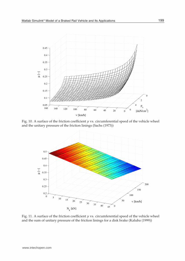
In Fig. 10 a surface of the friction coefficient μ vs. circumferential speed of the vehicle wheeland the unitary pressure of the friction linings for a block brake is shown.

For the disk brake the friction coefficient μ has been determined on the basis of the resultspresented in Kaluba (1999). In Fig. 11 a surface of the friction coefficient μ vs. circumferentialspeed of the vehicle wheel and the sum of unitary pressure of the friction linings for a diskbrake is shown.


www.intechopen.com


020406080100120140160

0

2

4

6

0.05

0.1

0.15

0.2

0.25

0.3

0.35

0.4

0.45

px

[daN/cm2]

v [km/h]

µ [

−]

Fig. 10. A surface of the friction coefficient μ vs. circumferential speed of the vehicle wheeland the unitary pressure of the friction linings (Sachs (1973))

05

1015

2025

3035

4045 0

50

100

150

200

0.2

0.25

0.3

0.35

0.4

0.45

0.5

v [km/h]

Nk [kN]

µ [

−]

Fig. 11. A surface of the friction coefficient μ vs. circumferential speed of the vehicle wheeland the sum of unitary pressure of the friction linings for a disk brake (Kaluba (1999))


www.intechopen.com


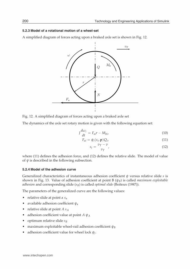
5.2.3 Model of a rotational motion of a wheel-set

A simplified diagram of forces acting upon a braked axle set is shown in Fig. 12.

Q

N

Fa

ω

Mb

r

vT

Fig. 12. A simplified diagram of forces acting upon a braked axle set

The dynamics of the axle set rotary motion is given with the following equation set:

Jdωi

dt= Fair − Mbi, (10)

Fai = ψi(si, p)Qi, (11)

si =vT − v

vT, (12)

where (11) defines the adhesion force, and (12) defines the relative slide. The model of valueof ψ is described in the following subsection.

5.2.4 Model of the adhesion curve

Generalized characteristics of instantaneous adhesion coefficient ψ versus relative slide s isshown in Fig. 13. Value of adhesion coefficient at point B (ψB) is called maximum exploitableadhesion and corresponding slide (sB) is called optimal slide (Boiteux (1987)).

The parameters of the generalized curve are the following values:

• relative slide at point α sα

• available adhesion coefficient ψα

• relative slide at point A sA

• adhesion coefficient value at point A ψA

• optimum relative slide sB

• maximum exploitable wheel-rail adhesion coefficient ψB

• adhesion coefficient value for wheel lock ψl .


www.intechopen.com


s[−]

ψ

ψB

0sα sA sB

ψα

ψA

ψl

wheellock

α

B

A

1

Fig. 13. Generalized characteristics of instantaneous coefficient of adhesion ψ versus relativeslide s (ORE (1985))

The shape and parameters of the curve depend on many factors, most of which are difficultor impossible to establish. The most important factors are listed below (Boiteux (1987; 1990;1998); ORE (1985; 1990)):

• state of the rail

• vehicle velocity vT

• absolute wheel slide σ

• relative wheel slide s

• circumferential deceleration of the wheels d

• slide energy E developed in the wheel and a rail contact point.

The mathematical model of adhesion coefficient, based on Boiteux (1987; 1990; 1998); ORE(1985; 1990), is described in detail in Barna (2009).

As an example, according to Boiteux (1987), maximum exploitable wheel-rail adhesioncoefficient ψB and optimum relative slide sB can be estimated with the following equations:

ψB = k

√

Q ψα Eo

2 dm, (13)

and

sB =1

vT

√

2 Eo dm

Q ψα. (14)

One of the most important behavior of the adhesion curve, which has been taken intoconsideration is, that during the braking at low adhesion with efficiently operating WSP


www.intechopen.com


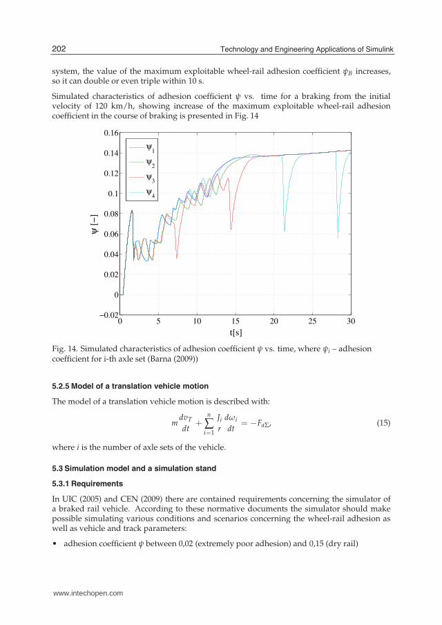
system, the value of the maximum exploitable wheel-rail adhesion coefficient ψB increases,so it can double or even triple within 10 s.

Simulated characteristics of adhesion coefficient ψ vs. time for a braking from the initialvelocity of 120 km/h, showing increase of the maximum exploitable wheel-rail adhesioncoefficient in the course of braking is presented in Fig. 14

0 5 10 15 20 25 30−0.02

0

0.02

0.04

0.06

0.08

0.1

0.12

0.14

0.16

t[s]

ψ [

−]

ψ1

ψ2

ψ3

ψ4

Fig. 14. Simulated characteristics of adhesion coefficient ψ vs. time, where ψi – adhesioncoefficient for i-th axle set (Barna (2009))

5.2.5 Model of a translation vehicle motion

The model of a translation vehicle motion is described with:

mdvT

dt+

n

∑i=1

Ji

r

dωi

dt= −FaΣ, (15)

where i is the number of axle sets of the vehicle.

5.3 Simulation model and a simulation stand

5.3.1 Requirements

In UIC (2005) and CEN (2009) there are contained requirements concerning the simulator ofa braked rail vehicle. According to these normative documents the simulator should makepossible simulating various conditions and scenarios concerning the wheel-rail adhesion aswell as vehicle and track parameters:

• adhesion coefficient ψ between 0,02 (extremely poor adhesion) and 0,15 (dry rail)


www.intechopen.com


• adhesion variation as occurs in real life

• sudden changes of adhesion as the ones occurring when a wheel encounters a spilled oilor dead leaves

• dynamic variation of wheel-rail adhesion coefficient vs. vehicle velocity and the slidecontrolled by WSP system

• maximum rail slope of 50‰

• drag braking test (when a vehicle is hauled at constant speed).

Simulator should make possible modeling the vehicles of the following parameters:

• vehicle velocity up to 240 km/h

• changes of parameters such as wheel diameter and inertia of axle sets, mass of the vehicleand particular bogies as well as location of the centroid, loading with passenger or cargoas well as braking force characteristics

• various brake positions with braking rate values λ being within the range 25% do 200%(for the braking systems independent of adhesion)

• braking systems which, apart from the friction brake are additionally equipped with thebrake independent of adhesion, e.g. track brake

It is recommended, that for the traction vehicles it should be possible to simulate blending(electrodynamic brake cooperating with friction brake).

5.3.2 Simulation model

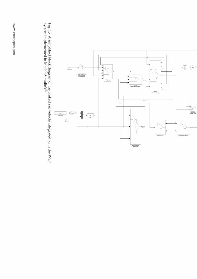
The simulation model of the braked rail vehicle integrated with the WSP system has been

implemented in Matlab Simulink�. A simplified block diagram of the model is shown inFig. 15. Validation of the model is basically performed by comparing the braking distancesobtained from simulations performed with the experimental results (CEN (2009); UIC (2005)).

5.3.3 Simulation stands

In the Figures 16, 17 i 18 block diagrams showing various possibilities of realizing thelaboratory test stand have been shown.

In Fig. 16 a stand described in UIC (2005) and CEN (2009) is shown, in which the computersimulation is minimized. This stand comprises a hardware model of a brake system withdump valves installed and pressure sensors mounted in brake cylinders. These pressurevalues are read by the analog inputs of the computer vehicle simulator, which calculates theadhesion forces and resulting wheel velocities. Fast analog output or counter output board ofthe computer vehicle simulator outputs pulse train simulating impulses from the WSP speedsensors.

A real WSP controlling device inputs the simulated speed signals from the computer vehiclesimulator and outputs signals controlling dump valves in the hardware model of a brakesystem. The advantage of this stand is fidelity of simulating the pneumatic part of the vehiclebraking system, which makes possible obtaining accurate values of brake cylinder pressuresduring WSP operation. The disadvantage is relatively high cost of the stand.

In Fig. 17 another version of a test stand is shown in which, comparing to the previous stand,also the pneumatic system is computer simulated. A reliable model of a pneumatic system


www.intechopen.com

16

Will-b

e-s

et-b

y-IN

-TE

CH

0.06

pmax[kPa]

385

lh

STOP

Sterowanie zaworowStan zaworow

Regulatorprzeciwposlizgowy

Przetwornikobr−imp 10ms

Obliczaniepredkosci referencyjnej

Model zaworowupustowych

Modelzestawu kolowego

Modelukladu hamulcowego

Losowa zmianawspolczynnikaprzyczepnosci

Krzywaprzyczepnosci

1s

1s

1000

−1/m

Fcn

f(u)

Clock

10ms

100ms

vT

vT4

Tp1..6

4

4

s1..6

4

4

vzest 1..6

t

t

t

2

p

4

4

pcyl1..6

4

ZO

4

ZL

4

4

4

4

4

44

4

Mh1..6

4

4

4

4

4 4 psi

4

4

4

E0

4

4

0

Fig

.15.A

simp

lified

blo

ckd

iagram

of

the

brak

edrail

veh

iclein

tegrated

with

the

WS

Psy

stemim

plem

ented

inM

atlabS

imu

link�

204Technology and Engineering Applications of Simulink

ww

w.intechopen.com


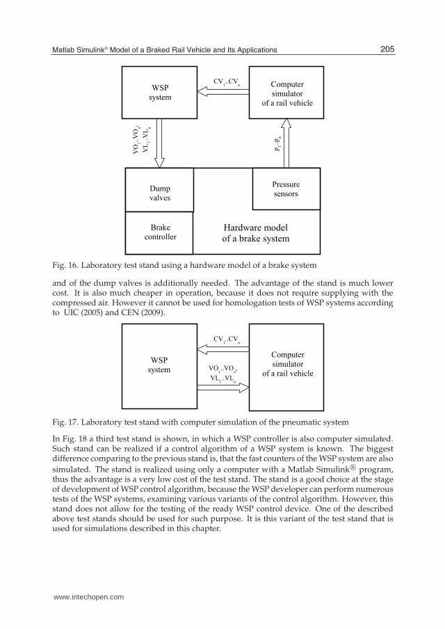
Fig. 16. Laboratory test stand using a hardware model of a brake system

and of the dump valves is additionally needed. The advantage of the stand is much lowercost. It is also much cheaper in operation, because it does not require supplying with thecompressed air. However it cannot be used for homologation tests of WSP systems accordingto UIC (2005) and CEN (2009).

Fig. 17. Laboratory test stand with computer simulation of the pneumatic system

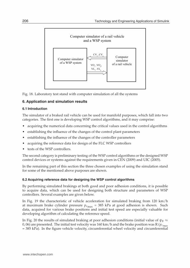
In Fig. 18 a third test stand is shown, in which a WSP controller is also computer simulated.Such stand can be realized if a control algorithm of a WSP system is known. The biggestdifference comparing to the previous stand is, that the fast counters of the WSP system are also

simulated. The stand is realized using only a computer with a Matlab Simulink� program,thus the advantage is a very low cost of the test stand. The stand is a good choice at the stageof development of WSP control algorithm, because the WSP developer can perform numeroustests of the WSP systems, examining various variants of the control algorithm. However, thisstand does not allow for the testing of the ready WSP control device. One of the describedabove test stands should be used for such purpose. It is this variant of the test stand that isused for simulations described in this chapter.


www.intechopen.com


Fig. 18. Laboratory test stand with computer simulation of all the systems

6. Application and simulation results

6.1 Introduction

The simulator of a braked rail vehicle can be used for manifold purposes, which fall into twocategories. The first one is developing WSP control algorithms, and it may comprise:

• acquiring the numerical data concerning the critical values used in the control algorithms

• establishing the influence of the changes of the control plant parameters

• establishing the influence of the changes of the controller parameters

• acquiring the reference data for design of the FLC WSP controllers

• tests of the WSP controllers.

The second category is preliminary testing of the WSP control algorithms or the designed WSPcontrol devices or systems against the requirements given in CEN (2009) and UIC (2005).

In the remaining part of this section the three chosen examples of using the simulation standfor some of the mentioned above purposes are shown.

6.2 Acquiring reference data for designing the WSP control algorithms

By performing simulated brakings at both good and poor adhesion conditions, it is possibleto acquire data, which can be used for designing both structure and parameters of WSPcontrollers. Several examples are given below.

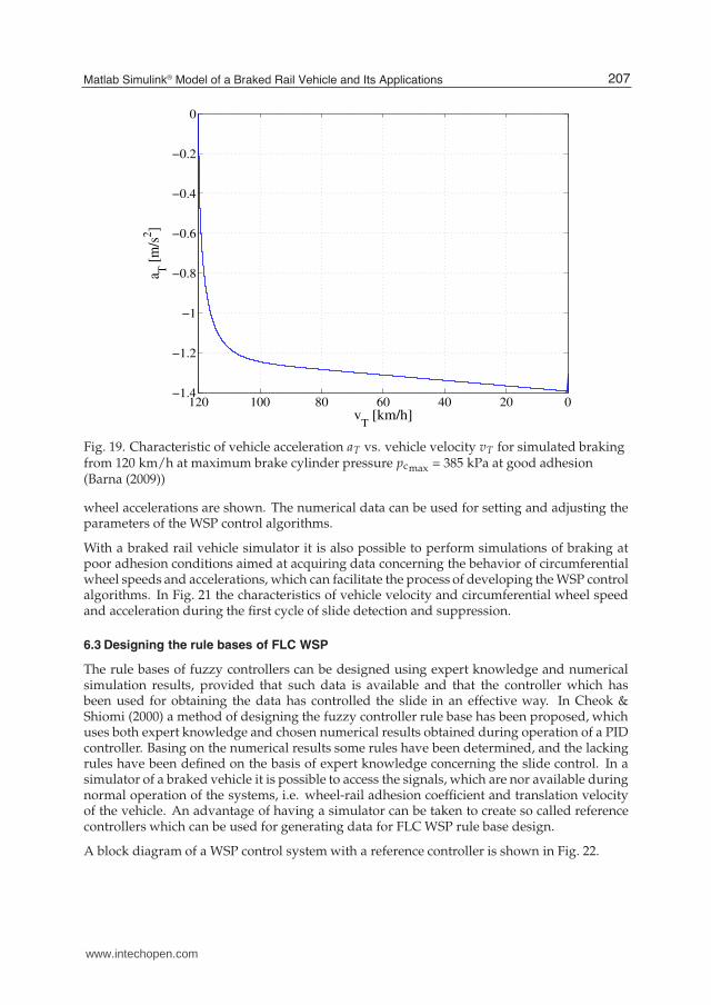
In Fig. 19 the characteristic of vehicle acceleration for simulated braking from 120 km/hat maximum brake cylinder pressure pcmax = 385 kPa at good adhesion is shown. Suchdata, acquired for various brake positions and initial test speed are especially valuable fordeveloping algorithm of calculating the reference speed.

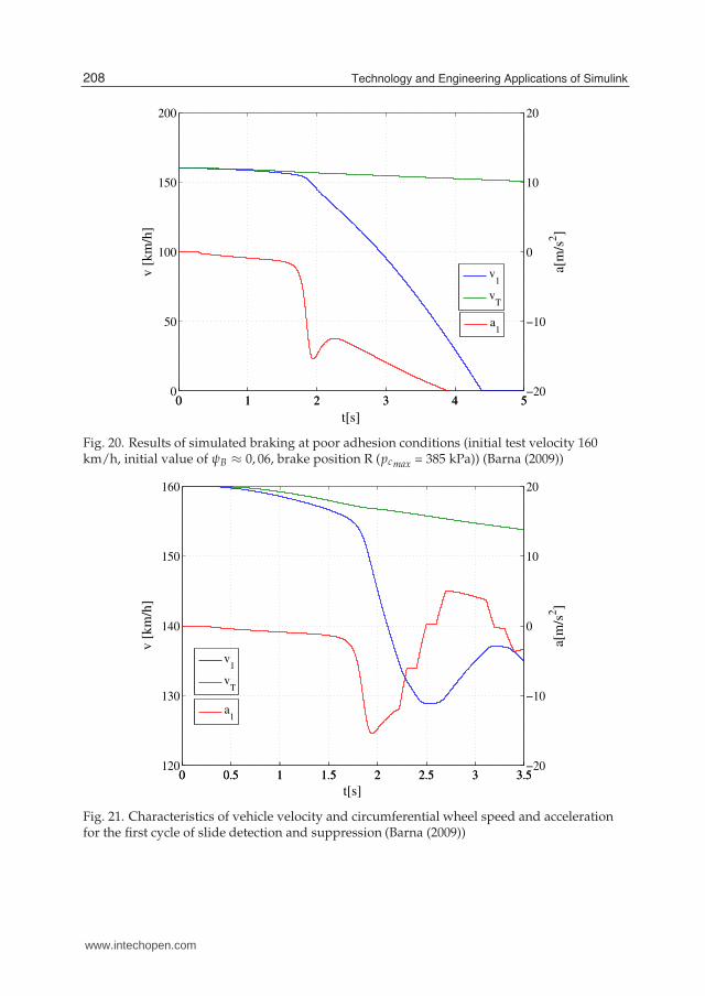
In Fig. 20 the results of simulated braking at poor adhesion conditions (initial value of ψB ≈

0, 06) are presented. The initial test velocity was 160 km/h and the brake position was R (pcmax= 385 kPa). In the figure vehicle velocity, circumferential wheel velocity and circumferential


www.intechopen.com


020406080100120−1.4

−1.2

−1

−0.8

−0.6

−0.4

−0.2

0

vT [km/h]

a T [

m/s

2]

Fig. 19. Characteristic of vehicle acceleration aT vs. vehicle velocity vT for simulated brakingfrom 120 km/h at maximum brake cylinder pressure pcmax = 385 kPa at good adhesion(Barna (2009))

wheel accelerations are shown. The numerical data can be used for setting and adjusting theparameters of the WSP control algorithms.

With a braked rail vehicle simulator it is also possible to perform simulations of braking atpoor adhesion conditions aimed at acquiring data concerning the behavior of circumferentialwheel speeds and accelerations, which can facilitate the process of developing the WSP controlalgorithms. In Fig. 21 the characteristics of vehicle velocity and circumferential wheel speedand acceleration during the first cycle of slide detection and suppression.

6.3 Designing the rule bases of FLC WSP

The rule bases of fuzzy controllers can be designed using expert knowledge and numericalsimulation results, provided that such data is available and that the controller which hasbeen used for obtaining the data has controlled the slide in an effective way. In Cheok &Shiomi (2000) a method of designing the fuzzy controller rule base has been proposed, whichuses both expert knowledge and chosen numerical results obtained during operation of a PIDcontroller. Basing on the numerical results some rules have been determined, and the lackingrules have been defined on the basis of expert knowledge concerning the slide control. In asimulator of a braked vehicle it is possible to access the signals, which are nor available duringnormal operation of the systems, i.e. wheel-rail adhesion coefficient and translation velocityof the vehicle. An advantage of having a simulator can be taken to create so called referencecontrollers which can be used for generating data for FLC WSP rule base design.

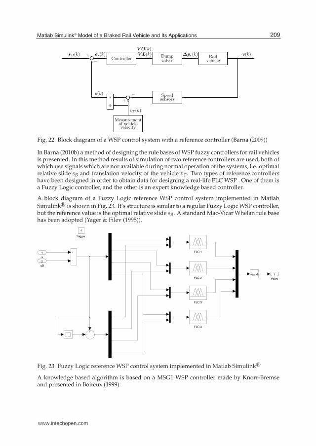
A block diagram of a WSP control system with a reference controller is shown in Fig. 22.


www.intechopen.com


0 1 2 3 4 50

50

100

150

200

t[s]

v [

km

/h]

v1

vT

0 1 2 3 4 5−20

−10

0

10

20

a[m

/s2]

a1

Fig. 20. Results of simulated braking at poor adhesion conditions (initial test velocity 160km/h, initial value of ψB ≈ 0, 06, brake position R (pcmax = 385 kPa)) (Barna (2009))

0 0.5 1 1.5 2 2.5 3 3.5120

130

140

150

160

v [

km

/h]

v1

vT

0 0.5 1 1.5 2 2.5 3 3.5−20

−10

0

10

20

t[s]

a[m

/s2]

a1

Fig. 21. Characteristics of vehicle velocity and circumferential wheel speed and accelerationfor the first cycle of slide detection and suppression (Barna (2009))


www.intechopen.com


sB(k) es(k)V O(k),V L(k) ∆pc(k) v(k)+

−Controller

Dumpvalves

Railvehicle

Speedsensors

Measurementof vehiclevelocity

+

−∗

÷

vT (k)

s(k)

Fig. 22. Block diagram of a WSP control system with a reference controller (Barna (2009))

In Barna (2010b) a method of designing the rule bases of WSP fuzzy controllers for rail vehiclesis presented. In this method results of simulation of two reference controllers are used, both ofwhich use signals which are nor available during normal operation of the systems, i.e. optimalrelative slide sB and translation velocity of the vehicle vT. Two types of reference controllershave been designed in order to obtain data for designing a real-life FLC WSP . One of them isa Fuzzy Logic controller, and the other is an expert knowledge based controller.

A block diagram of a Fuzzy Logic reference WSP control system implemented in Matlab

Simulink� is shown in Fig. 23. It’s structure is similar to a regular Fuzzy Logic WSP controller,but the reference value is the optimal relative slide sB. A standard Mac-Vicar Whelan rule basehas been adopted (Yager & Filev (1995)).

Valve

1round

FLC 4

FLC 3

FLC 2

FLC 1

Trigger

sB

2

s

1

Fig. 23. Fuzzy Logic reference WSP control system implemented in Matlab Simulink�

A knowledge based algorithm is based on a MSG1 WSP controller made by Knorr-Bremseand presented in Boiteux (1999).


www.intechopen.com


The input controller values for each axle set are:

• absolute wheel slide σ

• circumferential wheel acceleration a.

The output controller values are the same as in the Fuzzy Logic controllers described earlier.Three reference functions are defined, which divide the slide space into four ranges versusthe reference velocity vre f : ∆σ1(vre f ), ∆σ2(vre f ) and ∆σ3(vre f ). These functions are shown inFig. 24.

∆σ1 = f(vref )

∆σ2 = f(vref )

∆σ3 = f(vref )

vref

∆σ

Fig. 24. Reference values of absolute slide used in control algorithm of MSG1 WSPsystem (Boiteux (1999))

Four values of circumferential wheel accelerations are also defined: a1, a2, a3 oraz a4. Thesevalues are demonstratively pictured in Fig. 25.

t

a

a1

a2a3

a4

Fig. 25. Values of circumferential wheel accelerations used in control algorithm of MSG1WSP system pictured demonstratively (Boiteux (1999))

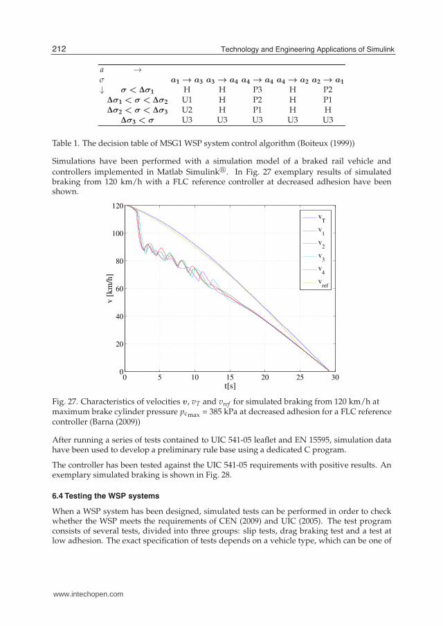
The decision table of MSG1 WSP system control algorithm is presented in Table 1.

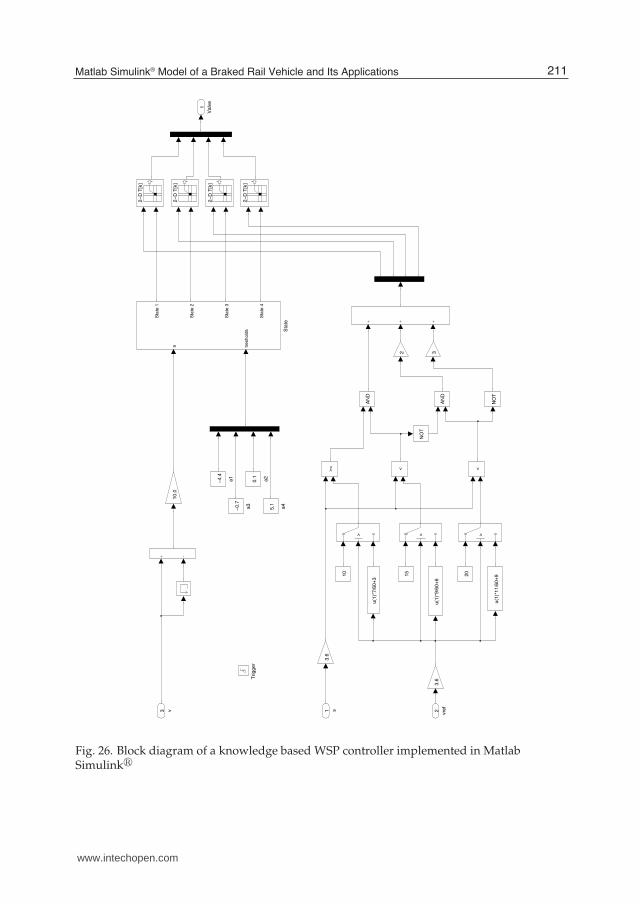
A block diagram of a knowledge based WSP control system implemented in Matlab

Simulink� is shown in Fig. 26.


www.intechopen.com


Valv

e

1

20

a4

5.1a3

−0.7

a2

0.1

10

15

a1

−4.4

>

>

>

Sta

te

a tre

sh

old

s

Sta

te 1

Sta

te 2

Sta

te 3

Sta

te 4

<<>=

NO

T

NO

T

AN

D

AN

D

10.0

3.6

32

3.6

u(1

)*7/6

0+

3

u(1

)*9/6

0+

6

u(1

)*11/6

0+

9

2−

D T

[k]

2−

D T

[k]

2−

D T

[k]

2−

D T

[k]

Trigger

v3

vre

f

2s1

Fig. 26. Block diagram of a knowledge based WSP controller implemented in MatlabSimulink�


www.intechopen.com


a →

σ a1 → a3 a3 → a4 a4 → a4 a4 → a2 a2 → a1

↓ σ < ∆σ1 H H P3 H P2∆σ1 < σ < ∆σ2 U1 H P2 H P1∆σ2 < σ < ∆σ3 U2 H P1 H H

∆σ3 < σ U3 U3 U3 U3 U3

Table 1. The decision table of MSG1 WSP system control algorithm (Boiteux (1999))

Simulations have been performed with a simulation model of a braked rail vehicle and

controllers implemented in Matlab Simulink�. In Fig. 27 exemplary results of simulatedbraking from 120 km/h with a FLC reference controller at decreased adhesion have beenshown.

0 5 10 15 20 25 300

20

40

60

80

100

120

t[s]

v [

km

/h]

vT

v1

v2

v3

v4

vref

Fig. 27. Characteristics of velocities v, vT and vref for simulated braking from 120 km/h atmaximum brake cylinder pressure pcmax = 385 kPa at decreased adhesion for a FLC referencecontroller (Barna (2009))

After running a series of tests contained to UIC 541-05 leaflet and EN 15595, simulation datahave been used to develop a preliminary rule base using a dedicated C program.

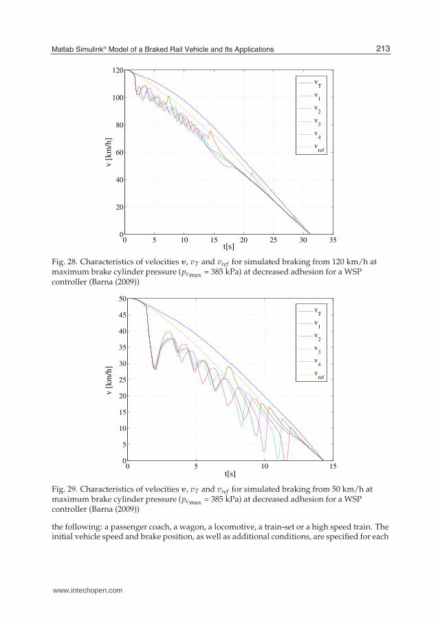
The controller has been tested against the UIC 541-05 requirements with positive results. Anexemplary simulated braking is shown in Fig. 28.

6.4 Testing the WSP systems

When a WSP system has been designed, simulated tests can be performed in order to checkwhether the WSP meets the requirements of CEN (2009) and UIC (2005). The test programconsists of several tests, divided into three groups: slip tests, drag braking test and a test atlow adhesion. The exact specification of tests depends on a vehicle type, which can be one of


www.intechopen.com


0 5 10 15 20 25 30 350

20

40

60

80

100

120

t[s]

v [

km

/h]

vT

v1

v2

v3

v4

vref

Fig. 28. Characteristics of velocities v, vT and vref for simulated braking from 120 km/h atmaximum brake cylinder pressure (pcmax = 385 kPa) at decreased adhesion for a WSPcontroller (Barna (2009))

0 5 10 150

5

10

15

20

25

30

35

40

45

50

t[s]

v [

km

/h]

vT

v1

v2

v3

v4

vref

Fig. 29. Characteristics of velocities v, vT and vref for simulated braking from 50 km/h atmaximum brake cylinder pressure (pcmax = 385 kPa) at decreased adhesion for a WSPcontroller (Barna (2009))

the following: a passenger coach, a wagon, a locomotive, a train-set or a high speed train. Theinitial vehicle speed and brake position, as well as additional conditions, are specified for each


www.intechopen.com


test. In order to check whether a WSP meets the requirements of the normative documents,appropriate simulated tests should be performed, and the results assessed.

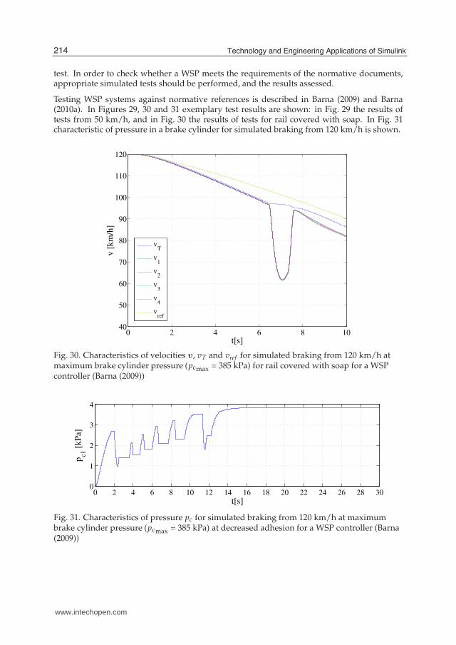
Testing WSP systems against normative references is described in Barna (2009) and Barna(2010a). In Figures 29, 30 and 31 exemplary test results are shown: in Fig. 29 the results oftests from 50 km/h, and in Fig. 30 the results of tests for rail covered with soap. In Fig. 31characteristic of pressure in a brake cylinder for simulated braking from 120 km/h is shown.

0 2 4 6 8 1040

50

60

70

80

90

100

110

120

t[s]

v [

km

/h]

vT

v1

v2

v3

v4

vref

Fig. 30. Characteristics of velocities v, vT and vref for simulated braking from 120 km/h atmaximum brake cylinder pressure (pcmax = 385 kPa) for rail covered with soap for a WSPcontroller (Barna (2009))

0 2 4 6 8 10 12 14 16 18 20 22 24 26 28 300

1

2

3

4

t[s]

pc1

[kP

a]

Fig. 31. Characteristics of pressure pc for simulated braking from 120 km/h at maximumbrake cylinder pressure (pcmax = 385 kPa) at decreased adhesion for a WSP controller (Barna(2009))


www.intechopen.com


7. Conclusions

In order to design an efficient WSP controller, a simulator of a braked rail vehicleis indispensable. The mathematical model of the wheel-rail adhesion must compriseregeneration of adhesion by controlled slide.

The simulator can be used for manifold purposes, including developing and testing of WSPcontrollers.

One of possible applications is using the simulation results of the reference controllers fordesigning the rule bases for WSP FLC controllers. From the analysis of performance ofthe WSP fuzzy controller, the rule base of which has been designed in this way, it can beconcluded, that this method makes possible designing efficient controllers.

The test program realized by the simulator must comply with the requirements of CEN (2009)and UIC (2005), thus making possible testing of the controllers in the whole possible range ofslide and acceleration values.

The futer research concerning the simulator of the braked rail vehicle would comprise:

• further development of the mathematical model of particular sub-models, especially themodel of the adhesion coefficient and model of the pneumatic system

• developing a software/hardware simulator with xPCTarget toolbox using a computerfitted with I/O boards.

8. Acknowledgements

This paper has been produced as part of the Research Projects "Microprocessor based Anti-slipSystem for traction rail vehicles meeting the requirements of Technical Specifications ofInteroperability" N R10 0046 06/2009 with the financial support of the Ministry of Scienceand Higher Education.

9. List of symbols

a [m/s2] – circumferential wheel accelerationaT [m/s2] – vehicle accelerationAk [m

2] – area of piston of the brake cylinderAx [m2] – area of friction surface of the brake diskdm [m/s2] – average value of circumferential wheel deceleration from the beginning of

braking and the moment when the slide value reaches 0.4e [−] – control errorE [J] – instantaneous value of axle set slide energy, from the start of the braking until

the instant moment tEo [J] – value of axle set slide energy from the start of braking until reaching of the

working point (s, ψ) point BFf [N] – force of the return spring of the brake cylinder

Fa [N] – adhesion force for an axle setFaΣ [N] – sum of adhesion forces for all axle sets of a vehicleip [−] – final ratio of clamp mechanisms of an axle setJ [kg m2] – moment of inertia of rotating elements associated with an axle set, reduced to

the axle set axis


www.intechopen.com


Lh [m] – total braking distanceMb [Nm] – braking torque of an axle setm [kg] – vehicle massN [N] – vertical rail reaction force for an axle setNk [N] – pressure exerted by brake discs, reduced to the braking radiusn [−] – number of axle sets of a vehiclepc [Pa] – brake cylinder pressurep [−] – vector of parameters of ψ vs. s characteristicspcmax [Pa] – maximum pressure in a brake cylinder for a given brake positionpcin [Pa] – instantaneous air pressure at inlet of a dump valvepc0 [Pa] – outlet dump valve air pressure value at the moment of change of the dump

valve statepx [daN/cm2] – unitary pressure of the friction linings of a brake blockQ [N] – instantaneous load of the axle setr [m] – wheel radiusrb [m] – brake radiusrd [m] – brake disk radiuss [−] – relative slide of wheels against the railssB [−] – optimum relative slidesα [−] – relative slide for point αt [s] – timeTh [s] – total time of braking until standstillTV [s] – time constant of dump valve ventingTF [s] – time constant of dump valve fillingv [km/h] – circumferential velocity of axle set wheelsvre f [km/h] – vehicle reference velocity

vT [km/h] – vehicle velocityγ [−] – coefficient of rotational massηr [−] – coefficient of increasing the efficiency of the lever mechanism of the brake

clamp mechanism in motionηs [−] – static efficiency of the lever mechanism of the brake clamp mechanismλ [−] – braking rateμ [−] – friction coefficient of the brake block friction liningψ [−] – instantaneous value of wheel-rail adhesion coefficientψB [−] – maximum exploitable wheel-rail adhesion coefficientψl [−] – adhesion coefficient for locked wheelsψα [−] – available adhesion coefficientσ [km/h] – absolute slide of wheels against the railsσ [km/h] – estimated absolute slide of wheels against the railsω [rad/s] – angular velocity of a vehicle axle set

10. References

Barna, G. (2009). Control Algorithms of Wheel Slide Protection Systems for Rail Vehicles (in Polish),PhD thesis, Poznan University of Technology.

Barna, G. (2010a). Simulation based design and tests of wheel slide protection systems forrail vehicles, Application of System Science, Computer Science, Academic PublishingHouse EXIT, Warsaw, pp. 271–280.


www.intechopen.com


Barna, G. (2010b). Simulation based design of fuzzy wheel slide protection controller forrail vehicles, Proceedings of 15th International Conference on Methods and Models inAutomation and Robotics, Miedzyzdroje.

Barna, G. & Kaluba, M. (2009). Safety and reliability of microprocessor brake control systemsfor multiple units, Proceedings of XI International Conference QSEV 2009 (Quality, Safetyand Ecology in Transport), Kraków.

Boiteux, M. (1987). Influence de l’énergie de glissment sur l’adhérence exploitable en freinage,Revue Générale des Chemins de Fer 106(October): 05–15.

Boiteux, M. (1990). Influence de l’énergie de glissment sur l’adhérence exploitable en freinage,Revue Générale des Chemins de Fer 109(Juillet - Août): 31–38.

Boiteux, M. (1998). Le problème de l’adhérence en freinage, Chemins de Fer 5(452): 28–39.Boiteux, M. (1999). Auxiliaires sophistiqués du freinage d’aujourd’hui — les antienrayeurs,

Chemins de Fer 6(459): 24–35.Caldara, C., Rivera, M. G. & Poma, G. (1996). Software implementation of an anti-skidding

control system for traction electrical drives based on fuzzy-identification techniques,Symposium on Power Electronics, Industrial Drives, Power Quality, Traction Systems,Capri, pp. C3–19 – C3–25.

CEN (2009). EN 15595, Railway applications — Braking — Wheel Slide Protection.Cheok, A. D. & Shiomi, S. (2000). Combined heuristic knowledge and limited measurement

based fuzzy logic antiskid control for railway applications, IEEE Transactions onSystems, Man, and Cybernetics — Part C: Applications and Reviews 30(4).

Jergéus, J. (1998). Martensite formation and residual stresses around railway wheel flats, ProcInsts Mech Engrs, Vol. 212, pp. 69–79.

Kaczorek, T. (1977). Theory of Automatic Control Systems (in Polish), WNT, Warszawa.Kaluba, M. (1999). Influence of selected factors upon developing of the phenomenon of fluid friction in

the disk brakes of rail vehicles (in Polish), PhD thesis, Poznan University of Technology.Knorr Bremse AG. (2002). Bremsen für Schienenfahrzeuge; Handbuch Bremstechnische Begriffe und

Werte, Knorr Bremse AG.Kwasnikowski, J. & Firlik, B. (2006). Excessive wear of the wheel treads of the rail bus,

Proceedings of 17th Scientific Conference ”Rail Vehicles”, Kazimierz Dolny, pp. 413–422.Mauer, G. F. (1995). A fuzzy logic controller for an ABS braking system, IEEE Transactions on

Fuzzy Systems 3(4): 381–388.Ofierzynski, M. (2008). The method of automatic generation of a model for dynamic-running

calculations of rail vehicles (in polish), Proceedings of 18th Scientific Conference ”RailVehicles”, Vol. 2, Katowice – Ustron, pp. 392 – 412.

ORE (1985). Adhesion During Braking and Anti-skid Devices, ORE B 164, RP 1, Synthesis ofCurrent Knowledge Concerning Adhesion, Office for Research and Experiments of theInternational Union of Railways, Utrecht.

ORE (1990). Adhesion During Braking and Anti-skid Devices, ORE B 164, RP 2, Fundamental Lawsof Adhesion in braking, Office for Research and Experiments of the International Unionof Railways, Utrecht.

Pawełczyk, M. (2008). Mathematical model of a system: wheel with a flat spot – rail,Proceedings of 18th Scientific Conference ”Rail Vehicles”, Vol. 2, Katowice – Ustron,pp. 425 – 434.

Sachs, K. (1973). Elektrische Triebfahrzeuge, Vol. 1, 2 edn, Springer-Verlag, Wien New York.Sanz, M. G. R. R. & Pérez-Rodríguez, J. (1997). An antislipping fuzzy logic controller for a

railway traction system, Proceedings of the sixth IEEE International Conference on FuzzySystems, Barcelona.


www.intechopen.com


Tao, G. & Kokotovic, P. (1996). Adaptive control of systems with actuator and sensor nonlinearities,John Wiley Sons, Inc., New York.

UIC (2005). UIC 541-05, Brakes — Specifications for the Construction of Various Brake Parts —Wheel Slide Protection Device (WSP), 2 edn.

Will, A. B. & Zak, S. H. (2000). Antilock brake system modelling and fuzzy control, Int. J.Vehicle Design 24(1): 01–18.

Yager, R. R. & Filev, D. P. (1995). Essentials of Fuzzy Modeling and Control, Wiley-Interscience,New York.


www.intechopen.com

Technology and Engineering Applications of SimulinkEdited by Prof. Subhas Chakravarty

ISBN 978-953-51-0635-7Hard cover, 256 pagesPublisher InTechPublished online 23, May, 2012Published in print edition May, 2012

InTech EuropeUniversity Campus STeP Ri Slavka Krautzeka 83/A 51000 Rijeka, Croatia Phone: +385 (51) 770 447 Fax: +385 (51) 686 166www.intechopen.com

InTech ChinaUnit 405, Office Block, Hotel Equatorial Shanghai No.65, Yan An Road (West), Shanghai, 200040, China

Phone: +86-21-62489820 Fax: +86-21-62489821

Building on MATLAB (the language of technical computing), Simulink provides a platform for engineers to plan,model, design, simulate, test and implement complex electromechanical, dynamic control, signal processingand communication systems. Simulink-Matlab combination is very useful for developing algorithms, GUIassisted creation of block diagrams and realisation of interactive simulation based designs. The elevenchapters of the book demonstrate the power and capabilities of Simulink to solve engineering problems withvaried degree of complexity in the virtual environment.

How to referenceIn order to correctly reference this scholarly work, feel free to copy and paste the following:

Grażyna Barna (2012). Matlab Simulink(r) Model of a Braked Rail Vehicle and Its Applications, Technology andEngineering Applications of Simulink, Prof. Subhas Chakravarty (Ed.), ISBN: 978-953-51-0635-7, InTech,Available from: http://www.intechopen.com/books/technology-and-engineering-applications-of-simulink/matlab-simulink-model-of-a-braked-rail-vehicle-and-its-applications

© 2012 The Author(s). Licensee IntechOpen. This is an open access articledistributed under the terms of the Creative Commons Attribution 3.0License, which permits unrestricted use, distribution, and reproduction inany medium, provided the original work is properly cited.

http://creativecommons.org/licenses/by/3.0

Matlab Simulink Model of a Braked Rail Vehicle and Its ...

Documents

Transcript of Matlab Simulink Model of a Braked Rail Vehicle and Its ...