MATLAB SIMSCAPE manual
153
Simscape™ 3 User’s Guide
description
tutorial matlab simulink simscape modulein the book are included some examples useful to create own models
Transcript of MATLAB SIMSCAPE manual

Simscape™ 3User’s Guide

How to Contact The MathWorks
www.mathworks.com Webcomp.soft-sys.matlab Newsgroupwww.mathworks.com/contact_TS.html Technical Support
[email protected] Product enhancement [email protected] Bug [email protected] Documentation error [email protected] Order status, license renewals, [email protected] Sales, pricing, and general information
508-647-7000 (Phone)
508-647-7001 (Fax)
The MathWorks, Inc.3 Apple Hill DriveNatick, MA 01760-2098For contact information about worldwide offices, see the MathWorks Web site.
Simscape™ User’s Guide
© COPYRIGHT 2007–2010 by The MathWorks, Inc.The software described in this document is furnished under a license agreement. The software may be usedor copied only under the terms of the license agreement. No part of this manual may be photocopied orreproduced in any form without prior written consent from The MathWorks, Inc.
FEDERAL ACQUISITION: This provision applies to all acquisitions of the Program and Documentationby, for, or through the federal government of the United States. By accepting delivery of the Programor Documentation, the government hereby agrees that this software or documentation qualifies ascommercial computer software or commercial computer software documentation as such terms are usedor defined in FAR 12.212, DFARS Part 227.72, and DFARS 252.227-7014. Accordingly, the terms andconditions of this Agreement and only those rights specified in this Agreement, shall pertain to and governthe use, modification, reproduction, release, performance, display, and disclosure of the Program andDocumentation by the federal government (or other entity acquiring for or through the federal government)and shall supersede any conflicting contractual terms or conditions. If this License fails to meet thegovernment’s needs or is inconsistent in any respect with federal procurement law, the government agreesto return the Program and Documentation, unused, to The MathWorks, Inc.
Trademarks
MATLAB and Simulink are registered trademarks of The MathWorks, Inc. Seewww.mathworks.com/trademarks for a list of additional trademarks. Other product or brandnames may be trademarks or registered trademarks of their respective holders.
Patents
The MathWorks products are protected by one or more U.S. patents. Please seewww.mathworks.com/patents for more information.

Revision HistoryMarch 2007 Online only New for Version 1.0 (Release 2007a)September 2007 Online only Revised for Version 2.0 (Release 2007b)March 2008 Online only Revised for Version 2.1 (Release 2008a)October 2008 Online only Revised for Version 3.0 (Release 2008b)March 2009 Online only Revised for Version 3.1 (Release 2009a)September 2009 Online only Revised for Version 3.2 (Release 2009b)March 2010 Online only Revised for Version 3.3 (Release 2010a)


Contents
Modeling Physical Systems
1Basic Principles of Modeling Physical Networks . . . . . 1-2Overview of the Physical Network Approach to ModelingPhysical Systems . . . . . . . . . . . . . . . . . . . . . . . . . . . . . . . 1-2
Variable Types . . . . . . . . . . . . . . . . . . . . . . . . . . . . . . . . . . . . 1-4Building the Mathematical Model . . . . . . . . . . . . . . . . . . . . 1-5Direction of Variables . . . . . . . . . . . . . . . . . . . . . . . . . . . . . 1-6Connector Ports and Connection Lines . . . . . . . . . . . . . . . . 1-8Connecting Simscape Diagrams to Simulink Sources andScopes . . . . . . . . . . . . . . . . . . . . . . . . . . . . . . . . . . . . . . . . 1-10
Introducing the Simscape Block Libraries . . . . . . . . . . . 1-11Library Structure Overview . . . . . . . . . . . . . . . . . . . . . . . . . 1-11Using the Simulink Library Browser to Access the BlockLibraries . . . . . . . . . . . . . . . . . . . . . . . . . . . . . . . . . . . . . . 1-11
Using the Command Prompt to Access the BlockLibraries . . . . . . . . . . . . . . . . . . . . . . . . . . . . . . . . . . . . . . 1-12
Essential Steps to Building a Physical Model . . . . . . . . . 1-14Building Your Model . . . . . . . . . . . . . . . . . . . . . . . . . . . . . . . 1-14Using the Conserving Ports . . . . . . . . . . . . . . . . . . . . . . . . . 1-15Using the Physical Signal Ports . . . . . . . . . . . . . . . . . . . . . . 1-16
Creating a Simple Model . . . . . . . . . . . . . . . . . . . . . . . . . . . 1-17Building a Simscape Diagram . . . . . . . . . . . . . . . . . . . . . . . 1-17Modifying Initial Settings . . . . . . . . . . . . . . . . . . . . . . . . . . . 1-25Running the Simulation . . . . . . . . . . . . . . . . . . . . . . . . . . . . 1-26Adjusting the Parameters . . . . . . . . . . . . . . . . . . . . . . . . . . . 1-29
Modeling Best Practices . . . . . . . . . . . . . . . . . . . . . . . . . . . . 1-35Grounding Rules . . . . . . . . . . . . . . . . . . . . . . . . . . . . . . . . . . 1-35Avoiding Numerical Simulation Issues . . . . . . . . . . . . . . . . 1-38
Modeling Pneumatic Systems . . . . . . . . . . . . . . . . . . . . . . . 1-42
v

Intended Applications . . . . . . . . . . . . . . . . . . . . . . . . . . . . . . 1-42Assumptions and Limitations . . . . . . . . . . . . . . . . . . . . . . . 1-42Fundamental Equations . . . . . . . . . . . . . . . . . . . . . . . . . . . . 1-43Network Variables . . . . . . . . . . . . . . . . . . . . . . . . . . . . . . . . 1-44Connection Constraints . . . . . . . . . . . . . . . . . . . . . . . . . . . . 1-45References . . . . . . . . . . . . . . . . . . . . . . . . . . . . . . . . . . . . . . . 1-45
Simulating Physical Models
2How Simscape Simulation Works . . . . . . . . . . . . . . . . . . . 2-2Simscape Simulation Phases . . . . . . . . . . . . . . . . . . . . . . . . 2-2Model Validation . . . . . . . . . . . . . . . . . . . . . . . . . . . . . . . . . . 2-4Network Construction . . . . . . . . . . . . . . . . . . . . . . . . . . . . . . 2-4Equation Construction . . . . . . . . . . . . . . . . . . . . . . . . . . . . . 2-5Computing Initial Conditions . . . . . . . . . . . . . . . . . . . . . . . . 2-5Performing Transient Initialization . . . . . . . . . . . . . . . . . . . 2-6Transient Solve . . . . . . . . . . . . . . . . . . . . . . . . . . . . . . . . . . . 2-6
Working with Solvers . . . . . . . . . . . . . . . . . . . . . . . . . . . . . . 2-8Selecting a Solver . . . . . . . . . . . . . . . . . . . . . . . . . . . . . . . . . 2-8Input Filtering . . . . . . . . . . . . . . . . . . . . . . . . . . . . . . . . . . . . 2-10
Troubleshooting Simulation Errors . . . . . . . . . . . . . . . . . 2-13Troubleshooting Tips and Techniques . . . . . . . . . . . . . . . . . 2-13System Configuration Errors . . . . . . . . . . . . . . . . . . . . . . . . 2-14Numerical Simulation Issues . . . . . . . . . . . . . . . . . . . . . . . . 2-17Initial Conditions Solve Failure . . . . . . . . . . . . . . . . . . . . . . 2-19Transient Simulation Issues . . . . . . . . . . . . . . . . . . . . . . . . 2-20
Finding an Operating Point . . . . . . . . . . . . . . . . . . . . . . . . 2-22What Is an Operating Point? . . . . . . . . . . . . . . . . . . . . . . . . 2-22How to Find Operating Points . . . . . . . . . . . . . . . . . . . . . . . 2-23Finding Operating Points with Simscape, Simulink, andRelated Products . . . . . . . . . . . . . . . . . . . . . . . . . . . . . . . . 2-24
Linearizing at an Operating Point . . . . . . . . . . . . . . . . . . 2-28What Is Linearization? . . . . . . . . . . . . . . . . . . . . . . . . . . . . . 2-28How to Linearize a Model . . . . . . . . . . . . . . . . . . . . . . . . . . . 2-30
vi Contents

Linearizing a Model with Simscape, Simulink, and RelatedProducts . . . . . . . . . . . . . . . . . . . . . . . . . . . . . . . . . . . . . . . 2-30
References . . . . . . . . . . . . . . . . . . . . . . . . . . . . . . . . . . . . . . . 2-34
Generating Code . . . . . . . . . . . . . . . . . . . . . . . . . . . . . . . . . . 2-35About Code Generation from Simscape Models . . . . . . . . . 2-35Related Simulink Code Generation Documentation . . . . . . 2-35Reasons for Generating Code . . . . . . . . . . . . . . . . . . . . . . . . 2-36Using Code-Related Products and Features . . . . . . . . . . . . 2-36How Simscape Code Generation Differs from Simulink . . . 2-37
Limitations . . . . . . . . . . . . . . . . . . . . . . . . . . . . . . . . . . . . . . . 2-39Sample Time and Solver Restrictions . . . . . . . . . . . . . . . . . 2-39Algebraic Loops . . . . . . . . . . . . . . . . . . . . . . . . . . . . . . . . . . . 2-39Restricted Simulink Tools . . . . . . . . . . . . . . . . . . . . . . . . . . 2-40Unsupported Simulink Tools . . . . . . . . . . . . . . . . . . . . . . . . 2-42Simulink Tools Not Compatible with Simscape Blocks . . . 2-42Code Generation . . . . . . . . . . . . . . . . . . . . . . . . . . . . . . . . . . 2-42
Logging Simulation Data
3About Simulation Data Logging . . . . . . . . . . . . . . . . . . . . . 3-2Suggested Workflows . . . . . . . . . . . . . . . . . . . . . . . . . . . . . . 3-2Limitations . . . . . . . . . . . . . . . . . . . . . . . . . . . . . . . . . . . . . . 3-2
How to Log Simulation Data . . . . . . . . . . . . . . . . . . . . . . . . 3-3How to Enable Data Logging . . . . . . . . . . . . . . . . . . . . . . . . 3-3Data Logging Options . . . . . . . . . . . . . . . . . . . . . . . . . . . . . . 3-4
Data Logging Example . . . . . . . . . . . . . . . . . . . . . . . . . . . . . 3-6
vii
Working with Physical Units
4Overview . . . . . . . . . . . . . . . . . . . . . . . . . . . . . . . . . . . . . . . . . 4-2
Unit Definitions . . . . . . . . . . . . . . . . . . . . . . . . . . . . . . . . . . . 4-4
Specifying Units in Block Dialogs . . . . . . . . . . . . . . . . . . . 4-9
Thermal Unit Conversions . . . . . . . . . . . . . . . . . . . . . . . . . . 4-11About Affine Units . . . . . . . . . . . . . . . . . . . . . . . . . . . . . . . . 4-11When to Apply Affine Conversion . . . . . . . . . . . . . . . . . . . . 4-11How to Apply Affine Conversion . . . . . . . . . . . . . . . . . . . . . 4-12
Angular Units . . . . . . . . . . . . . . . . . . . . . . . . . . . . . . . . . . . . . 4-14References . . . . . . . . . . . . . . . . . . . . . . . . . . . . . . . . . . . . . . . 4-14
Using the Simscape Editing Mode
5About the Simscape Editing Mode . . . . . . . . . . . . . . . . . . . 5-2Suggested Workflows . . . . . . . . . . . . . . . . . . . . . . . . . . . . . . 5-2What You Can Do in Restricted Mode . . . . . . . . . . . . . . . . . 5-3What You Can Do in Full Mode . . . . . . . . . . . . . . . . . . . . . . 5-4Switching Between Modes . . . . . . . . . . . . . . . . . . . . . . . . . . 5-4Working with Block Libraries . . . . . . . . . . . . . . . . . . . . . . . 5-7
Working with Restricted and Full Modes . . . . . . . . . . . . 5-9Setting the Model Loading Preference . . . . . . . . . . . . . . . . . 5-9Saving a Model in Restricted Mode . . . . . . . . . . . . . . . . . . . 5-10Working with a Model in Restricted Mode . . . . . . . . . . . . . 5-13Switching from Restricted to Full Mode . . . . . . . . . . . . . . . 5-21
Editing Mode Information . . . . . . . . . . . . . . . . . . . . . . . . . . 5-23What Is the Current Mode? . . . . . . . . . . . . . . . . . . . . . . . . . 5-23Which Licenses Are Checked Out? . . . . . . . . . . . . . . . . . . . . 5-23
viii Contents
Examples
AGetting Started . . . . . . . . . . . . . . . . . . . . . . . . . . . . . . . . . . . . A-2
Best Practices . . . . . . . . . . . . . . . . . . . . . . . . . . . . . . . . . . . . . A-2
Editing Mode . . . . . . . . . . . . . . . . . . . . . . . . . . . . . . . . . . . . . . A-2
Index
ix

x Contents

1
Modeling Physical Systems
• “Basic Principles of Modeling Physical Networks” on page 1-2
• “Introducing the Simscape Block Libraries” on page 1-11
• “Essential Steps to Building a Physical Model” on page 1-14
• “Creating a Simple Model” on page 1-17
• “Modeling Best Practices” on page 1-35
• “Modeling Pneumatic Systems” on page 1-42
1 Modeling Physical Systems
Basic Principles of Modeling Physical Networks
In this section...
“Overview of the Physical Network Approach to Modeling Physical Systems”on page 1-2
“Variable Types” on page 1-4
“Building the Mathematical Model” on page 1-5
“Direction of Variables ” on page 1-6
“Connector Ports and Connection Lines” on page 1-8
“Connecting Simscape Diagrams to Simulink Sources and Scopes” on page1-10
Overview of the Physical Network Approach toModeling Physical SystemsSimscape™ software is a set of block libraries and special simulation featuresfor modeling physical systems in the Simulink® environment. It employsthe Physical Network approach, which differs from the standard Simulinkmodeling approach and is particularly suited to simulating systems thatconsist of real physical components.
Simulink blocks represent basic mathematical operations. When youconnect Simulink blocks together, the resulting diagram is equivalent to themathematical model, or representation, of the system under design. Simscapetechnology lets you create a network representation of the system underdesign, based on the Physical Network approach. According to this approach,each system is represented as consisting of functional elements that interactwith each other by exchanging energy through their ports.
These connection ports are bidirectional. They mimic physical connectionsbetween elements. Connecting Simscape blocks together is analogous toconnecting real components, such as pumps, valves, and so on. In other words,Simscape diagrams mimic the physical system layout. If physical componentscan be connected, their models can be connected, too. You do not have tospecify flow directions and information flow when connecting Simscapeblocks, just as you do not have to specify this information when you connect
1-2

Basic Principles of Modeling Physical Networks
real physical components. The Physical Network approach, with its Throughand Across variables and bidirectional physical connections, automaticallyresolves all the traditional issues with variables, directionality, and so on.
The number of connection ports for each element is determined by the numberof energy flows it exchanges with other elements in the system, and dependson the level of idealization. For example, a fixed-displacement hydraulicpump in its simplest form can be represented as a two-port element, with oneenergy flow associated with the inlet (suction) and the other with the outlet.In this representation, the angular velocity of the driving shaft is assumedconstant, making it possible to neglect the energy exchange between thepump and the shaft. To account for a variable driving torque, you need a thirdport associated with the driving shaft.
An energy flow is characterized by its variables. Each energy flow isassociated with two variables, one Through and one Across (see “VariableTypes” on page 1-4 for more information). Usually, these are the variableswhose product is the energy flow in watts. They are called the basic, orconjugate, variables. For example, the basic variables for mechanicaltranslational systems are force and velocity, for mechanical rotationalsystems—torque and angular velocity, for hydraulic systems—flow rate andpressure, for electrical systems—current and voltage.
The following example illustrates a Physical Network representation of adouble-acting hydraulic cylinder.
The element is represented with three energy flows: two flows of hydraulicenergy through the inlet and outlet of the cylinder and a flow of mechanical
1-3

1 Modeling Physical Systems
energy associated with the rod motion. It therefore has the following threeconnector ports:
• A — Hydraulic conserving port associated with pressure p1 (an Acrossvariable) and flow rate q1 (a Through variable)
• B — Hydraulic conserving port associated with pressure p2 (an Acrossvariable) and flow rate q2 (a Through variable)
• R — Mechanical translational conserving port associated with rod velocityv3 (an Across variable) and force F3 (a Through variable)
See “Connector Ports and Connection Lines” on page 1-8 for more informationon connector port types.
Variable TypesPhysical Network approach supports two types of variables:
• Through — Variables that are measured with a gauge connected in seriesto an element.
• Across — Variables that are measured with a gauge connected in parallelto an element.
The following table lists the Through and Across variables associated witheach type of physical domain in Simscape software:
Physical Domain Across Variable Through Variable
Electrical Voltage Current
Hydraulic Pressure Flow rate
Magnetic Magnetomotive force(mmf)
Flux
Mechanical rotational Angular velocity Torque
Mechanicaltranslational
Translational velocity Force
1-4

Basic Principles of Modeling Physical Networks
Physical Domain Across Variable Through Variable
Pneumatic Pressure andtemperature
Mass flow rate and heatflow
Thermal Temperature Heat flow
Note Generally, the product of each pair of Across and Through variablesassociated with a domain is power (energy flow in watts). The exceptions arepneumatic domain, where the product of pressure and mass flow rate is notpower, and magnetic domain, where the product of mmf and flux is not power,but energy. These result in a pseudo-bond graph.
Building the Mathematical ModelThrough and Across variables associated with all the energy flows form thebasis of the mathematical model of the block.
For example, the model of a double-acting hydraulic cylinder shown in theprevious illustration can be described with a simple set of equations:
F p A p A3 1 1 2 2= −i i
q A v1 1 3= i
q A v2 2 3= i
1-5

1 Modeling Physical Systems
where
q1,q2 Flow rates through ports A and B, respectively (Through variables)
p1,p2 Gauge pressures at ports A and B, respectively (Across variables)
A1,A2 Piston effective areas
F3 Rod force (Through variable)
v3 Rod velocity (Across variable)
The model could be considerably more complex, for example, it couldaccount for friction, fluid compressibility, inertia of the moving parts, andso on. For all these different mathematical models, however, the elementconfiguration (that is, the number and type of ports and the associatedThrough and Across variables) would remain the same, meaning that thePhysical Network approach lets you substitute models of different levels ofcomplexity without introducing any changes to the schematic. For example,you can start developing your system by using the Resistive Tube block fromthe Foundation library, which accounts only for friction losses. At a laterstage in development, you may want to account for fluid compressibility.You can then replace it with a Hydraulic Pipeline block, available withSimHydraulics® block libraries, or, depending on your application, even witha Segmented Pipeline block if you also need to account for fluid inertia. Thismodeling principle is called incremental modeling.
Direction of VariablesEach variable is characterized by its magnitude and sign. The sign is theresult of measurement orientation. The same variable can be positive ornegative, depending on the polarity of a measurement gauge. That is whyit is very important to apply exactly the same rule to all the variables inthe Physical Network.
Elements with only two ports are characterized with one pair of variables, aThrough variable and an Across variable. Since these variables are closelyrelated, their orientation is defined with one direction. For example, if anelement is oriented from port A to port B, it implies that the Through variable(TV) is positive if it “flows” from A to B, and the Across variable is determined
1-6

Basic Principles of Modeling Physical Networks
as AV = AVA – AVB, where AVA and AVB are the element node potentials or, inother words, the values of this Across variable at ports A and B, respectively.
This approach to the direction of variables has the following benefits:
• Provides a simple and consistent way to determine whether an element isactive or passive. Energy is one of the most important characteristics tobe determined during simulation. If the variables direction, or sign, isdetermined as described above, their product (that is, the energy) is positiveif the element consumes energy, and is negative if it provides energy to asystem. This rule is followed throughout the Simscape software.
• Simplifies the model description. Symbol A B is enough to specifyvariable polarity for both the Across and the Through variables.
• Lets you apply the oriented graph theory to network analysis and design.
As an example of variables direction rules, let us consider the Ideal ForceSource block. In this block, as in many other mechanical blocks, port C isassociated with the source reference point (case), and port R is associatedwith the rod.
1-7

1 Modeling Physical Systems
The block positive direction is from port C to port R. This means that the forceis positive if it acts in the direction from C to R, and causes bodies connectedto port R to accelerate in the positive direction. The relative velocity isdetermined as v = vC – vR, where vR, vC are the absolute velocities at ports Rand C, respectively, and it is negative if velocity at port R is greater than thatat port C. The power generated by the source is computed as the product offorce and velocity, and is negative if the source provides energy to the system.
All the elements in a network are divided into active and passive elements,depending on whether they deliver energy to the system or dissipate (or store)it. Active elements (force and velocity sources, flow rate and pressure sources,etc.) must be oriented strictly in accordance with the line of action or functionthat they are expected to perform in the system, while passive elements(dampers, resistors, springs, pipelines, etc.) can be oriented either way.
Connector Ports and Connection LinesSimscape blocks may have the following types of ports:
• Physical Conserving ports — Bidirectional ports (for example, hydraulicor mechanical) that represent physical connections and relate physicalvariables based on the Physical Network approach.
• Physical Signal ports — Unidirectional ports transferring signals that usean internal Simscape engine for computations.
Each of these ports and connections between them are described in greaterdetail below.
1-8

Basic Principles of Modeling Physical Networks
Physical Conserving PortsSimscape blocks have special Conserving ports . You connect Conservingports with Physical connection lines, distinct from normal Simulink lines.Physical connection lines have no inherent directionality and represent theexchange of energy flows, according to the Physical Network approach.
• You can connect Conserving ports only to other Conserving ports of thesame type.
• The Physical connection lines that connect Conserving ports togetherare bidirectional lines that carry physical variables (Across and Throughvariables, as described above) rather than signals. You cannot connectPhysical lines to Simulink ports or to Physical Signal ports.
• Two directly connected Conserving ports must have the same values for alltheir Across variables (such as pressure or angular velocity).
• You can branch Physical connection lines. When you do so, componentsdirectly connected with one another continue to share the same Acrossvariables. Any Through variable (such as flow rate or torque) transferredalong the Physical connection line is divided among the multiplecomponents connected by the branches. How the Through variable isdivided is determined by the system dynamics.
For each Through variable, the sum of all its values flowing into a branchpoint equals the sum of all its values flowing out.
Each type of Physical Conserving ports used in Simscape blocks uniquelyrepresents a physical modeling domain. For a list of port types, along withthe Through and Across variables associated with each type, see the table in“Variable Types” on page 1-4.
Physical Signal PortsPhysical Signal ports carry signals between Simscape blocks. You connectthem with regular connection lines, similar to Simulink signal connections.Physical Signal ports are used in Simscape block diagrams instead ofSimulink input and output ports to increase computation speed and avoidissues with algebraic loops. Unlike Simulink signals, which are essentiallyunitless, physical signals can have units associated with them. You specifythe units along with the parameter values in the block dialogs, and Simscape
1-9

1 Modeling Physical Systems
software performs the necessary unit conversion operations when solving aphysical network.
Simscape Foundation library contains, among other sublibraries, a PhysicalSignals block library. These blocks perform math operations and otherfunctions on physical signals, and allow you to graphically implementequations inside the Physical Network.
Connecting Simscape Diagrams to Simulink Sourcesand ScopesSimscape block diagrams use physical signals instead of regular Simulinksignals. Therefore, you need converter blocks to connect Simscape diagramsto Simulink sources and scopes.
Use the Simulink-PS Converter block to connect Simulink sources or otherSimulink blocks to the inputs of a Physical Network diagram. You canalso use it to specify the input signal units. For more information, see theSimulink-PS Converter block reference page.
Use the PS-Simulink Converter block to connect outputs of a PhysicalNetwork diagram to Simulink scopes or other Simulink blocks. You can alsouse it to specify the desired output signal units. For more information, seethe PS-Simulink Converter block reference page.
For an example of using converter blocks to connect Simscape diagrams toSimulink sources and scopes, see “Creating a Simple Model” on page 1-17.
1-10

Introducing the Simscape™ Block Libraries
Introducing the Simscape Block Libraries
In this section...
“Library Structure Overview” on page 1-11
“Using the Simulink Library Browser to Access the Block Libraries” onpage 1-11
“Using the Command Prompt to Access the Block Libraries” on page 1-12
Library Structure OverviewSimscape block library contains two libraries that belong to the Simscapeproduct:
• Foundation library — Contains basic hydraulic, pneumatic, mechanical,electrical, magnetic, thermal, and physical signal blocks, organized intosublibraries according to technical discipline and function performed
• Utilities library — Contains essential environment blocks for creatingPhysical Networks models
In addition, if you have installed any of the add-on products of the PhysicalModeling family, you will see the corresponding libraries under the mainSimscape library.
You can combine all these blocks in your Simscape diagrams to model physicalsystems. You can also use the basic Simulink blocks in your diagrams, such assources or scopes. See “Connecting Simscape Diagrams to Simulink Sourcesand Scopes” on page 1-10 for more information on how to do this.
Using the Simulink Library Browser to Access theBlock LibrariesYou can access the blocks through the Simulink Library Browser. To displaythe Library Browser, click the Library Browser button in the toolbar of theMATLAB® desktop or Simulink model window:
1-11

1 Modeling Physical Systems
Alternatively, you can type simulink in the MATLAB Command Window.Then expand the Simscape entry in the contents tree.
For more information on using the Library Browser, see “Library Browser” inthe Simulink Graphical User Interface documentation.
Using the Command Prompt to Access the BlockLibrariesTo access individual block libraries by using the command prompt:
• To open the Simscape library, type simscape in the MATLAB CommandWindow.
• To open the main Simulink library (to access generic Simulink blocks), typesimulink in the MATLAB Command Window.
The Simscape library consists of two top-level libraries, Foundation andUtilities. In addition, if you have installed any of the add-on products of thePhysical Modeling family, you will see the corresponding libraries underSimscape library, as shown in the following illustration. Some of theselibraries contain second-level and third-level sublibraries. You can expand
1-12

Introducing the Simscape™ Block Libraries
each library by double-clicking its icon. For more details on library hierarchyand descriptions of block categories, see “Block Reference”.
1-13

1 Modeling Physical Systems
Essential Steps to Building a Physical Model
Building Your ModelThe rules that you must follow when building a physical model with Simscapesoftware are described in “Basic Principles of Modeling Physical Networks” onpage 1-2. This section briefly reviews these rules.
• Build your physical model by using a combination of blocks from theSimscape Foundation and Utilities libraries. Simscape software lets youcreate a network representation of the system under design, based on thePhysical Network approach. According to this approach, each system isrepresented as consisting of functional elements that interact with eachother by exchanging energy through their ports.
• Each Simscape diagram (or each topologically distinct physical network ina diagram) must contain a Solver Configuration block from the SimscapeUtilities library.
• If you have hydraulic elements in your model, the working fluid used inthe hydraulic circuit defines their global parameters, such as fluid density,fluid kinematic viscosity, fluid bulk modulus, and so on. To specify theworking fluid, attach a Custom Hydraulic Fluid block (or a Hydraulic Fluidblock, available with SimHydraulics block libraries) to each topologicallydistinct hydraulic circuit. If no Hydraulic Fluid block or Custom HydraulicFluid block is attached to a circuit, the hydraulic blocks use the defaultfluid, which is Skydrol LD-4 at 60°C and with a 0.005 ratio of entrapped air.
• If you have pneumatic elements in your model, default gas properties arefor dry air and ambient conditions of 101325 Pa and 20 degrees Celsius.Attach a Gas Properties block to each topologically distinct pneumaticcircuit to change gas properties and ambient conditions.
• To connect regular Simulink blocks (such as sources or scopes) to yourphysical network diagram, use the connector blocks, as described in “Usingthe Physical Signal Ports” on page 1-16.
• Use the incremental modeling approach. Start with a simple model, runand troubleshoot it, then add the desired special effects. For example, youcan start developing your system by using the Resistive Tube block fromthe Foundation library, which accounts only for friction losses. At a laterstage in development, you may want to account for fluid compressibility.
1-14
Essential Steps to Building a Physical Model
You can then replace it with a Hydraulic Pipeline block, available withSimHydraulics block libraries, or, depending on your application, even witha Segmented Pipeline block if you also need to account for fluid inertia. Forall these different mathematical models, the element configuration (thatis, the number and type of ports and the associated Through and Acrossvariables) would remain the same, meaning that the Physical Networkapproach lets you substitute models of different levels of complexitywithout introducing any changes to the schematic.
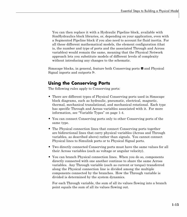
Simscape blocks, in general, feature both Conserving ports and PhysicalSignal inports and outports .
Using the Conserving PortsThe following rules apply to Conserving ports:
• There are different types of Physical Conserving ports used in Simscapeblock diagrams, such as hydraulic, pneumatic, electrical, magnetic,thermal, mechanical translational, and mechanical rotational. Each typehas specific Through and Across variables associated with it. For moreinformation, see “Variable Types” on page 1-4.
• You can connect Conserving ports only to other Conserving ports of thesame type.
• The Physical connection lines that connect Conserving ports togetherare bidirectional lines that carry physical variables (Across and Throughvariables, as described above) rather than signals. You cannot connectPhysical lines to Simulink ports or to Physical Signal ports.
• Two directly connected Conserving ports must have the same values for alltheir Across variables (such as voltage or angular velocity).
• You can branch Physical connection lines. When you do so, componentsdirectly connected with one another continue to share the same Acrossvariables. Any Through variable (such as current or torque) transferredalong the Physical connection line is divided among the multiplecomponents connected by the branches. How the Through variable isdivided is determined by the system dynamics.
For each Through variable, the sum of all its values flowing into a branchpoint equals the sum of all its values flowing out.
1-15

1 Modeling Physical Systems
Using the Physical Signal PortsThe following rules apply to Physical Signal ports:
• You can connect Physical Signal ports to other Physical Signal ports withregular connection lines, similar to Simulink signal connections. Theseconnection lines carry physical signals between Simscape blocks.
• You can connect Physical Signal ports to Simulink ports through specialconverter blocks. Use the Simulink-PS Converter block to connect Simulinkoutports to Physical Signal inports. Use the PS-Simulink Converter blockto connect Physical Signal outports to Simulink inports.
• Unlike Simulink signals, which are essentially unitless, Physical Signalscan have units associated with them. Simscape block dialogs let you specifythe units along with the parameter values, where appropriate. Use theconverter blocks to associate units with an input signal and to specify thedesired output signal units.
For examples of applying these rules when creating an actual physical model,see the following section, “Creating a Simple Model” on page 1-17.
1-16

Creating a Simple Model
Creating a Simple Model
In this section...
“Building a Simscape Diagram” on page 1-17
“Modifying Initial Settings” on page 1-25
“Running the Simulation” on page 1-26
“Adjusting the Parameters” on page 1-29
Building a Simscape DiagramIn this example, you are going to model a simple mechanical system andobserve its behavior under various conditions. This tutorial illustrates theessential steps to building a physical model, described in the previous section,and makes you familiar with using the basic Simscape blocks.
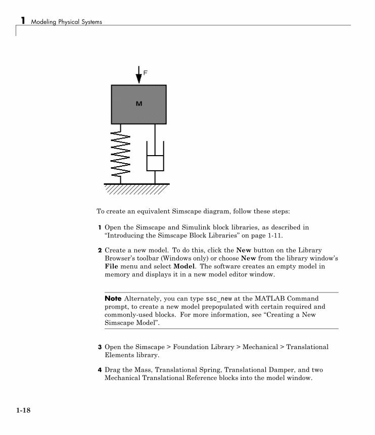
The following schematic represents a simple model of a car suspension. Itconsists of a spring and damper connected to a body (represented as a mass),which is agitated by a force. You can vary the model parameters, such as thestiffness of the spring, the mass of the body, or the force profile, and view theresulting changes to the velocity and position of the body.
1-17
1 Modeling Physical Systems
To create an equivalent Simscape diagram, follow these steps:
1 Open the Simscape and Simulink block libraries, as described in“Introducing the Simscape Block Libraries” on page 1-11.
2 Create a new model. To do this, click the New button on the LibraryBrowser’s toolbar (Windows only) or choose New from the library window’sFile menu and select Model. The software creates an empty model inmemory and displays it in a new model editor window.
Note Alternately, you can type ssc_new at the MATLAB Commandprompt, to create a new model prepopulated with certain required andcommonly-used blocks. For more information, see “Creating a NewSimscape Model”.
3 Open the Simscape > Foundation Library > Mechanical > TranslationalElements library.
4 Drag the Mass, Translational Spring, Translational Damper, and twoMechanical Translational Reference blocks into the model window.
1-18

Creating a Simple Model
5 Orient the blocks as shown in the following illustration. To rotate a block,select it and press Ctrl+R.
6 Connect the Translational Spring, Translational Damper, and Mass blocksto one of the Mechanical Translational Reference blocks as shown in thenext illustration.
1-19

1 Modeling Physical Systems
7 To add the representation of the force acting on the mass, open theSimscape > Foundation Library > Mechanical > Mechanical Sources libraryand add the Ideal Force Source block to your diagram.
To reflect the correct direction of the force shown in the original schematic,flip the block by selecting Format > Flip Block > Up-Down from the topmenu bar of the model window. Connect the block’s port C (for “case”) tothe second Mechanical Translational Reference block, and its port R (for“rod”) to the Mass block, as shown below.
1-20

Creating a Simple Model
8 Add the sensor to measure speed and position of the mass. Place the IdealTranslational Motion Sensor block from the Mechanical Sensors libraryinto your diagram and connect it as shown below.
1-21

1 Modeling Physical Systems
9 Now you need to add the sources and scopes. They are found in the regularSimulink libraries. Open the Simulink > Sources library and copy theSignal Builder block into the model. Then open the Simulink > Sinkslibrary and copy two Scope blocks. Rename one of the Scope blocks toVelocity and the other to Position.
1-22

Creating a Simple Model
10 Every time you connect a Simulink source or scope to a Simscape diagram,you have to use an appropriate converter block, to convert Simulink signalsinto physical signals and vice versa. Open the Simscape > Utilities libraryand copy a Simulink-PS Converter block and two PS-Simulink Converterblocks into the model. Connect the blocks as shown below.
1-23

1 Modeling Physical Systems
11 Each topologically distinct physical network in a diagram requiresexactly one Solver Configuration block, found in the Simscape > Utilitieslibrary. Copy this block into your model and connect it to the circuit bycreating a branching point and connecting it to the only port of the SolverConfiguration block. Your diagram now should look like this.
1-24

Creating a Simple Model
12 Your block diagram is now complete. Save it as simple_mech1.mdl.
Modifying Initial SettingsAfter you have put together a block diagram of your model, as described in theprevious section, you need to select a solver and provide the correct valuesfor configuration parameters.
To prepare for simulating the model, follow these steps:
1 Select a Simulink solver. On the top menu bar of the model window,select Simulation > Configuration Parameters. The ConfigurationParameters dialog box opens, showing the Solver node.
Under Solver options, set Solver to ode15s (Stiff/NDF) andMax stepsize to 0.2.
1-25

1 Modeling Physical Systems
Also note that Simulation time is specified to be between 0 and 10seconds. You can adjust this setting later, if needed.
Click OK to close the Configuration Parameters dialog box.
2 Save the model.
Running the SimulationAfter you’ve put together a block diagram and specified the initial settings foryour model, you can run the simulation.
1 The input signal for the force is provided by the Signal Builder block. Thesignal profile is shown in the illustration below. It starts with a value of 0,then at 4 seconds there is a step change to 1, and then it changes back to 0at 6 seconds. This is the default profile.
1-26

Creating a Simple Model
The Velocity scope outputs the mass velocity, and the Position scopeoutputs the mass displacement as a function of time. Double-click bothscopes to open them.
2 To run the simulation, click in the model window toolbar. The Simscapesolver evaluates the model, calculates the initial conditions, and runs thesimulation. For a detailed description of this process, see “How SimscapeSimulation Works” on page 2-2. Completion of this step may take a fewseconds. The message in the bottom-left corner of the model windowprovides the status update.
3 Once the simulation starts running, the Velocity and Position scopewindows display the simulation results, as shown in the next illustration.
1-27

1 Modeling Physical Systems
In the beginning, the mass is at rest. Then at 4 seconds, as the input signalchanges abruptly, the mass velocity spikes in the positive direction andgradually returns to zero. The mass position at the same time changesmore gradually, on account of inertia and damping, and stays at the newvalue as long as the force is acting upon it. At 6 seconds, when the inputsignal changes back to zero, the velocity gets a mirror spike, and the massgradually returns to its initial position.
1-28
Creating a Simple Model
You can now adjust various inputs and block parameters and see their effecton the mass velocity and displacement.
Adjusting the ParametersAfter running the initial simulation, you can experiment with adjustingvarious inputs and block parameters.
Try the following adjustments:
1 Change the force profile.
2 Change the model parameters.
3 Change the mass position output units.
Changing the Force ProfileThis example shows how a change in the input signal affects the force profile,and therefore the mass displacement.
1 Double-click the Signal Builder block to open it.
2 Click the first vertical segment of the signal profile and drag it from 4 to 2seconds, as shown below. Close the block dialog.
1-29

1 Modeling Physical Systems
3 Run the simulation. The simulation results are shown in the followingillustration.
1-30

Creating a Simple Model
Changing the Model ParametersIn our model, the force acts on a mass against a translational spring anddamper, connected in parallel. This example shows how changes in the springstiffness and damper viscosity affect the mass displacement.
1 Double-click the Translational Spring block. Set its Spring rate to 2000N/m.
1-31

1 Modeling Physical Systems
2 Run the simulation. The increase in spring stiffness results in smalleramplitude of mass displacement, as shown in the following illustration.
3 Next, double-click the Translational Damper block. Set its Dampingcoefficient to 500 N/(m/s).
4 Run the simulation. Because of the increase in viscosity, the mass is slowerboth in reaching its maximum displacement and in returning to the initialposition, as shown in the following illustration.
1-32

Creating a Simple Model
Changing the Mass Position Output UnitsIn our model, we have used the PS-Simulink Converter block in its defaultparameter configuration, which does not specify units. Therefore, thePosition scope outputs the mass displacement in the default length units,that is, in meters. This example shows how to change the output units for themass displacement to millimeters.
1 Double-click the PS-Simulink Converter block. Type mm in the Outputsignal unit combo box and click OK.
2 Run the simulation. In the Position scope window, click to autoscalethe scope axes. The mass displacement is now output in millimeters, asshown in the following illustration.
1-33

1 Modeling Physical Systems
1-34

Modeling Best Practices
Modeling Best Practices
In this section...
“Grounding Rules” on page 1-35
“Avoiding Numerical Simulation Issues” on page 1-38
Grounding RulesThis section contains guidelines for using domain-specific reference blocks(such as Electrical Reference, Mechanical Translational Reference, and soon) in Simscape diagrams, along with examples of correct and incorrectconfigurations.
Add reference blocks to your models according to the following rules:
• “Each Domain Requires at Least One Reference Block” on page 1-35
• “Each Circuit Requires at Least One Reference Block” on page 1-36
• “Multiple Connections to the Domain Reference Are Allowed Within aCircuit” on page 1-37
Each Domain Requires at Least One Reference BlockWithin a physical network, each domain must contain at least one referenceblock of the appropriate type. For example, the electromechanical modelshown in the following diagram has both Electrical Reference and RotationalReference blocks attached to the appropriate circuits.
1-35

1 Modeling Physical Systems
Each Circuit Requires at Least One Reference BlockEach topologically distinct circuit within a domain must contain at least onereference block. Some blocks, such as an Ideal Transformer, interface twoparts of the network but do not convey information about signal levels relativeto the reference block. In the following diagram, there are two separateelectrical circuits, and the Electrical Reference blocks are required on bothsides of the Ideal Transformer block.
1-36

Modeling Best Practices
The next diagram would produce an error because it is lacking an electricalreference in the circuit of the secondary winding.
The following diagram, however, will not produce an error because theresistor defines the output voltage relative to the ground reference.
Multiple Connections to the Domain Reference Are AllowedWithin a CircuitMore that one reference block may be used within a circuit to define multipleconnections to the domain reference:
1-37

1 Modeling Physical Systems
• Electrical conserving ports of all the blocks that are directly connected toground must be connected to an Electrical Reference block.
• All translational ports that are rigidly clamped to the frame (ground) mustbe connected to a Mechanical Translational Reference block.
• All rotational ports that are rigidly clamped to the frame (ground) must beconnected to a Mechanical Rotational Reference block.
• Hydraulic conserving ports of all the blocks that are referenced toatmosphere (for example, suction ports of hydraulic pumps, or return portsof valves, cylinders, pipelines, if they are considered directly connected toatmosphere) must be connected to a Hydraulic Reference block.
For example, the following diagram correctly indicates two separateconnections to an electrical ground.
Avoiding Numerical Simulation IssuesCertain configurations of physical modeling blocks can cause numericaldifficulties or slow down your simulation. When this happens, Simscapesolver issues a warning in the MATLAB workspace and, if it fails to initialize,a Simscape error.
1-38
Modeling Best Practices
In electrical circuits, common examples that can cause this behavior includevoltage sources connected in parallel with capacitors, inductors connected inseries with current sources, voltage sources connected in parallel, and currentsources connected in series. Often, the cause of the numerical difficulty isimmediately apparent. For example, two voltage sources in parallel musthave identical voltage values; otherwise, the ports connecting them would notbe physical conserving ports. In practical circuits, topologies such as parallelvoltage sources are possible, and small difference in their instantaneousvoltages is possible due to parasitic series resistance.
Note Mathematically, these topologies result in Index-2 differential algebraicequations (DAEs). Their solution requires two differentiations of theconstraint equations and, as such, it is numerically better to avoid thesecomponent topologies where possible.
There are two approaches to resolving these difficulties. The first is to changethe circuit to an equivalent simpler one. In the example of two parallel voltagesources, one source can be simply deleted. The same applies to two seriescurrent sources, the deleted one being replaced by a short circuit. For somecircuit topologies, however, it is not possible to find an equivalent simpler onethat resolves the problem, and the second approach is needed.
The second approach is to include small parasitic resistances in thecomponent. In the Simscape Foundation library, the Capacitor and Inductorblocks include such parasitic terms, so that you can connect capacitances inparallel with voltage sources and inductors in series with current sources. Ifyour circuit does not have any such topologies, then you can change the defaultparasitic terms to zero. Note that other blocks do not contain these parasiticterms, for example, the Mutual Inductor block. Therefore, if you wanted toconnect a mutual inductor primary in series with a current source, you wouldneed to introduce your own parasitic conductance across the primary winding.
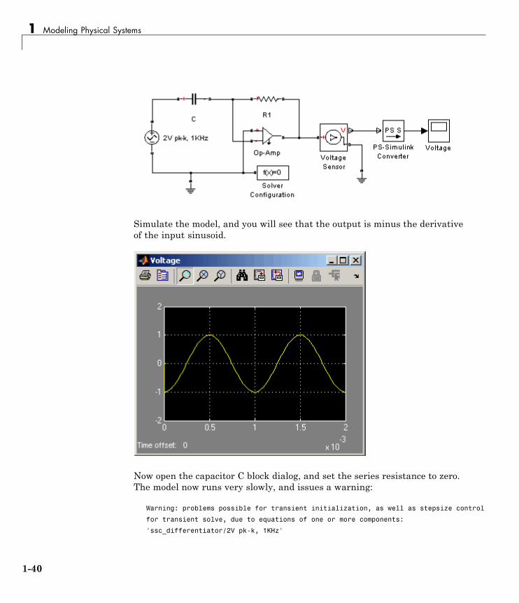
Example of Using a Parasitic Resistance to Avoid NumericalSimulation IssuesThe following diagram models a differentiator that might be used as part of aProportional-Integral-Derivative (PID) controller. You can open this model bytyping ssc_differentiator in the MATLAB Command Window.
1-39
1 Modeling Physical Systems
Simulate the model, and you will see that the output is minus the derivativeof the input sinusoid.
Now open the capacitor C block dialog, and set the series resistance to zero.The model now runs very slowly, and issues a warning:
Warning: problems possible for transient initialization, as well as stepsize control
for transient solve, due to equations of one or more components:
'ssc_differentiator/2V pk-k, 1KHz'
1-40

Modeling Best Practices
'ssc_differentiator/Op-Amp'
'ssc_differentiator/C'
The cause of the warning is that the circuit effectively connects the voltagesource in parallel with the capacitor. This is because an ideal op-ampsatisfies V+ = V- , where V+ and V- are the noninverting and inverting inputs,respectively. This is an example where it is not possible to replace the circuitwith an equivalent simpler one, and a parasitic small resistance has to beintroduced.
1-41

1 Modeling Physical Systems
Modeling Pneumatic Systems
In this section...
“Intended Applications” on page 1-42
“Assumptions and Limitations” on page 1-42
“Fundamental Equations” on page 1-43
“Network Variables” on page 1-44
“Connection Constraints” on page 1-45
“References” on page 1-45
Intended ApplicationsThe Foundation library contains basic pneumatic elements, such as orifices,chambers, and pneumatic-mechanical converters, as well as pneumaticsensors and sources. Use these blocks to model pneumatic systems, forapplications such as:
• Factory automation — basic pneumatic linear/rotational actuators, valves(variable orifices), and air supply
• Robotics — robotic arms and haptic interfaces
• Gaseous transportation systems and pipelines
You can also use these blocks to model dry air and low-pressure flows, forexample, for HVAC applications.
Assumptions and LimitationsPneumatic block models are based on the following assumptions:
• Working fluid is an ideal gas satisfying the ideal gas law.
• Specific heats at constant pressure and constant volume, cp and cv, areconstant.
1-42

Modeling Pneumatic Systems
• Processes are adiabatic, that is, there is no heat transfer betweencomponents and the environment (except for components with a separatethermal port).
• Gravitational effects can be neglected, that is, underlying equations containno head pressures due to gravity.
Fundamental EquationsThe energy balance for a control volume [1] is
dEdt
Q W m hv
gz m hv
gcvcv cv i i
ii
io o
o= − + + +⎛
⎝⎜⎜
⎞
⎠⎟⎟
⎛
⎝⎜⎜
⎞
⎠⎟⎟
− + +∑2 2
2 2zzo
o
⎛
⎝⎜⎜
⎞
⎠⎟⎟
⎛
⎝⎜⎜
⎞
⎠⎟⎟∑
where
Ecv Control volume total energy
Qcv Heat energy per second added to the gas through the boundary
Wcv Mechanical work per second performed by the gas
hi, ho Inlet and outlet enthalpies
vi, vo Gas inlet and outlet velocities
g Acceleration due to gravity
zi, zo Elevations at inlet and outlet ports
mi, mo Mass flow rates in and out of the control volume
The equation is an accounting balance for the energy of the control volume. Itstates that the rate of energy increase or decrease within the control volumeequals the difference between the rates of energy transfer in and out across theboundary. The mechanisms of energy transfer are heat and work, as for closedsystems, and the energy that accompanies the mass entering and exiting.
Pneumatic block models make several simplifying assumptions, as describedpreviously.
1-43
1 Modeling Physical Systems
The ideal gas law relates pressure, density, and temperature:
p RT= ρ
where
p Absolute pressure
ρ Gas density
R Specific gas constant
T Absolute gas temperature
Also, the specific enthalpies for an ideal gas at temperature T and constantpressure and constant volume are given by:
h c Tp=
h c Tv=
The pneumatic components also use the mass continuity equation:
ddt V
m mi oρ = −( )1
where ρ is the density of the gas within the component. For components withno internal mass of gas, the equation simplifies to:
G m mi o= =
where G is the mass flow rate through the component.
For specific equations used in each block, see the block reference pages.
Network VariablesThe Across variables are pressure and temperature, and the Throughvariables are mass flow rate and heat flow. Note that these choices result in
1-44

Modeling Pneumatic Systems
a pseudo-bond graph, because the product of pressure and mass flow rateis not power.
Connection ConstraintsEvery node in a pneumatic network must have a defined temperature aswell as pressure. This rule places some constraints on how you connectthe pneumatic elements. In effect, every node should have a volume offluid associated with it. When the ideal gas law is applied, this volumeof fluid determines the relationship between temperature and pressure.Some elements already have a volume of fluid associated with them, andtherefore having just one of these components connected to a node satisfiesthis condition. Such blocks include Constant Volume Pneumatic Chamber,Pneumatic Piston Chamber, Rotary Pneumatic Piston Chamber, andPneumatic Atmospheric Reference.
An exception to the above rule (that every node must have a volume of fluidassociated with it) occurs when two nodes are connected by a component forwhich the heat equation says that the temperatures are equal. In this case,just one of the nodes needs to be connected to a component with associatedvolume of fluid. Such components include the pressure and flow rate sources.
For models that represent an actual pneumatic network, these constraintsshould have no impact. For example, connecting two orifices in series makesno physical sense because the underlying assumption of the orifice equationis that gas is discharged into a volume of fluid. Therefore, modeling actualphysical systems should automatically satisfy these constraints.
References[1] Moran M.J. and Shapiro H.N. Fundamentals of EngineeringThermodynamics. Second edition. New York: John Wiley & Sons, 1992.
1-45

1 Modeling Physical Systems
1-46

2
Simulating Physical Models
• “How Simscape Simulation Works” on page 2-2
• “Working with Solvers” on page 2-8
• “Troubleshooting Simulation Errors” on page 2-13
• “Finding an Operating Point” on page 2-22
• “Linearizing at an Operating Point” on page 2-28
• “Generating Code” on page 2-35
• “Limitations” on page 2-39
2 Simulating Physical Models
How Simscape Simulation Works
In this section...
“Simscape Simulation Phases” on page 2-2
“Model Validation” on page 2-4
“Network Construction” on page 2-4
“Equation Construction” on page 2-5
“Computing Initial Conditions” on page 2-5
“Performing Transient Initialization” on page 2-6
“Transient Solve” on page 2-6
Simscape Simulation PhasesSimscape software gives you multiple ways to simulate and analyze physicalsystems in the Simulink environment. Running a physical model simulationis similar to running a simulation of any other Simulink model. It entailssetting various simulation options, starting the simulation, and viewing thesimulation results. See the Using Simulink documentation for a generaldiscussion of these topics. This chapter focuses on aspects of simulationspecific to Simscape and SimHydraulics models. Refer to the SimMechanics™and SimDriveline™ documentation for specifics of simulating and analyzingSimMechanics and SimDriveline models.
You might find this brief overview helpful for constructing models andunderstanding errors.
Simscape simulation sequence is shown in the following flow chart.
2-2

How Simscape™ Simulation Works
It consists of the following major phases:
1 “Model Validation” on page 2-4
2 “Network Construction” on page 2-4
3 “Equation Construction” on page 2-5
4 “Computing Initial Conditions” on page 2-5
2-3

2 Simulating Physical Models
5 “Performing Transient Initialization” on page 2-6
6 “Transient Solve” on page 2-6
Model ValidationSimscape solver first validates the model configuration and checks your dataentries from the block dialogs. In particular:
• Each topologically distinct physical network in a diagram requires exactlyone Solver Configuration block.
• If your model contains hydraulic elements, each topologically distincthydraulic circuit in a diagram requires a Custom Hydraulic Fluid block(or Hydraulic Fluid block, available with SimHydraulics block libraries)to be connected to it. These blocks define the fluid properties that act asglobal parameters for all the blocks connected to the hydraulic circuit. Ifno hydraulic fluid block is attached to a loop, the hydraulic blocks in thisloop use the default fluid. However, more than one hydraulic fluid block ina loop generates an error.
Similarly, if your model contains pneumatic elements, default gasproperties for a pneumatic network are for dry air and ambient conditionsof 101325 Pa and 20 degrees Celsius. Attaching a Gas Properties block to apneumatic circuit lets you change gas properties and ambient conditionsfor all the blocks connected to the circuit. However, more than one GasProperties block in a pneumatic circuit generates an error.
• Signal units specified in a Simulink-PS Converter block must matchthe input type expected by the Simscape block connected to it. Forexample, when you provide the input signal for an Ideal Angular VelocitySource block, specify angular velocity units, such as rad/s or rpm, in theSimulink-PS Converter block, or leave it unitless. Similarly, units specifiedin a PS-Simulink Converter block must match the type of physical signalprovided by the Simscape block outport.
Network ConstructionAfter validating the model, Simscape solver constructs the physical networkbased on the following principles:
• Two directly connected Conserving ports have the same values for all theirAcross variables (such as voltage or angular velocity).
2-4

How Simscape™ Simulation Works
• Any Through variable (such as current or torque) transferred alongthe Physical connection line is divided among the multiple componentsconnected by the branches. For each Through variable, the sum of all itsvalues flowing into a branch point equals the sum of all its values flowingout.
Equation ConstructionBased on the network configuration, the parameter values provided in theblock dialogs, and the global parameters defined by the fluid properties, ifapplicable, Simscape solver constructs the system of equations for the model.
These equations contain variables of the following types:
• Dynamic— Time derivative of this variable appears in equations. Dynamicvariables are the independent states for simulation.
• Algebraic— Time derivative of this variable does not appear in equations.Algebraic variables are always dependent (on dynamic variables, otheralgebraic variables, or inputs).
Computing Initial ConditionsSimscape solver computes the initial conditions only once, in the beginning ofsimulation (t=0).
Initial conditions are computed by setting all dynamic variables to 0, exceptthose corresponding to blocks that have an initial condition field in theirblock dialogs, and solving for all the system variables. The blocks with initialconditions have their dynamic variables set according to the user-providedvalue in the block dialog. Initial conditions can only be set on dynamicvariables, because these are the independent states for simulation. Forexample, the Translational Spring block has the Initial deformationparameter, so the corresponding spring position state is set to the initial offsetspecified in the block dialog. Refer to the block reference documentation tofind which blocks have initial conditions specified through their dialogs.
It is required that the initial conditions for dependent dynamic states be setconsistently. For example, the initial voltages on two parallel capacitors mustbe equal. When the solver detects dependent dynamic variables, it performs
2-5

2 Simulating Physical Models
a check and issues an error if the initial conditions on dynamic states arenot set consistently.
This concludes the initial conditions computation when the Start simulationfrom steady state check box in the Solver block dialog box is not selected(this is the default).
When this box is selected, the solver attempts to find the steady state thatwould result if the inputs to the system were held constant for a sufficientlylarge time, starting from the initial state obtained from the initial conditionscomputation, described previously. Although the solver tries to find theparticular steady state resulting from the given initial conditions, it isnot guaranteed to do so. All that is guaranteed is that if the steady-statesolve succeeds, the state found is a steady state (within tolerance). Steadystate means that the system variables are no longer changing with time.Simulation then starts from this steady state.
Note If the simulation fails at or near the start time when you use the Startsimulation from steady state option, consider clearing the check box andsimulating with the plain initial conditions computation only.
Performing Transient InitializationAfter computing the initial conditions, or after a subsequent event (such asa discontinuity resulting, for example, from a valve opening, or a hard stophitting the stop), Simscape solver performs transient initialization. This isdone by fixing all dynamic variables and solving for algebraic variables andderivatives of dynamic variables. The goal of transient initialization is toprovide a consistent set of initial conditions for the next transient solve phase.
Transient SolveFinally, Simscape solver performs transient solve of the system of equations.In transient solve, continuous differential equations are integrated in timeto compute all the variables as a function of time.
Simscape solver continues to perform the simulation according to the resultsof the transient solve until it encounters an event, such as a zero crossing or
2-6

How Simscape™ Simulation Works
discontinuity. The event may be within the physical network or elsewhere inthe Simulink model. If an event is encountered, Simscape solver returns tothe phase of transient initialization, and then back to transient solve. Thiscycle continues until the end of simulation.
2-7

2 Simulating Physical Models
Working with Solvers
In this section...
“Selecting a Solver” on page 2-8
“Input Filtering” on page 2-10
Selecting a SolverIt is possible to choose any variable-step or fixed-step solver for modelscontaining Simscape blocks. However, implicit solvers, such as ode14x,ode23t, and ode15s, are a better choice for a typical model. In particular,for stiff systems, implicit solvers typically take many fewer timesteps thanexplicit solvers, such as ode45, ode113, and ode1.
When you first create a model, the default Simulink solver is ode45. To selecta different solver, follow a procedure similar to that in “Modifying InitialSettings” on page 1-25.
If you do not modify the default solver and your system is stiff, yourperformance may not be optimal. To alert you to a potential issue, the systemissues a warning when you use an explicit solver in a model containingSimscape blocks. You can turn off this default warning or changed it to anerror for a particular model, by following these steps:
1 From the top menu bar in the model window, select Simulation >Configuration Parameters. The Configuration Parameters dialog boxopens.
2 In the left pane of the Configuration Parameters dialog box, selectSimscape.
2-8

Working with Solvers
3 Select the desired option from the Explicit solver used in modelcontaining Physical Networks blocks drop-down list:
• warning — Makes the system issue a warning upon simulation if themodel uses an explicit solver. This is the default option, designed to alertyou to a potential issue if you use the default solver.
• error— Makes the system issue an error upon simulation if the modeluses an explicit solver. If your model is stiff, and the use of explicitsolvers undesirable, you may choose to select this option to avoidtroubleshooting errors in the future.
• none — Turns off issuing a warning or error upon simulation withexplicit solver. For models that are not stiff, explicit solvers can beeffective, often taking fewer timesteps than implicit solvers. If you workwith such models and use explicit solvers, select this option to turn offthe warning upon simulation.
2-9

2 Simulating Physical Models
4 Click OK.
Input FilteringIf you use an explicit solver, you may need to provide time derivatives ofsome of the input signals. By default, needed input derivatives are providedby filtering the input through a low-pass filter. The derivative of the filteredinput can then be computed by the Physical Networks simulation engine.
You can control the way you provide time derivatives for each input signal byconfiguring the Simulink-PS Converter block connected to it:
1 Double-click the Simulink-PS Converter block to open its dialog box.
2 Click the Derivatives tab.
2-10

Working with Solvers
3 To avoid filtering the input signal, set Input derivatives parameter toFirst derivative of input user-provided.
When you select this option, a second Simulink input port appears on theSimulink-PS Converter block, to let you connect the signal providing inputderivatives. Input filtering is then turned off.
4 If you cannot provide the first derivative of the input signal as an additionalinput signal to the Simulink-PS Converter block, leave the Inputderivatives parameter set to No user-input provided derivatives. Inthis case, however, it is important to set the appropriate Input filteringtime constant parameter value for your model.
The filter time constant controls the filtering of the input signal. Thefiltered input follows the true input but is smoothed, with a lag on the orderof the time constant chosen. You should set the time constant to a valueno larger than the smallest time interval of interest in the system. Thetrade-off in choosing a very small time constant is that the filtered inputsignal will be closer to the true input signal, at the cost of increasing thestiffness of the system and slowing down the simulation.
Because input filtering can appreciably change the input signal anddrastically affect simulation results if the time constant is too large, awarning is issued when input filtering is used. The warning indicates whichSimulink-PS Converter blocks have their input signals filtered. You can turnoff this warning (or change it to an error) by changing the preferences on theSimscape pane of the Configuration Parameters dialog box:
1 From the top menu bar in the model window, select Simulation >Configuration Parameters. The Configuration Parameters dialog boxopens.
2 In the left pane of the Configuration Parameters dialog box, selectSimscape.
2-11
2 Simulating Physical Models
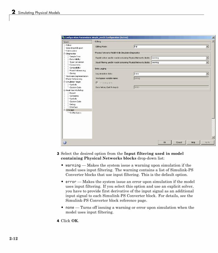
3 Select the desired option from the Input filtering used in modelcontaining Physical Networks blocks drop-down list:
• warning — Makes the system issue a warning upon simulation if themodel uses input filtering. The warning contains a list of Simulink-PSConverter blocks that use input filtering. This is the default option.
• error— Makes the system issue an error upon simulation if the modeluses input filtering. If you select this option and use an explicit solver,you have to provide first derivative of the input signal as an additionalinput signal to each Simulink-PS Converter block. For details, see theSimulink-PS Converter block reference page.
• none— Turns off issuing a warning or error upon simulation when themodel uses input filtering.
4 Click OK.
2-12

Troubleshooting Simulation Errors
Troubleshooting Simulation Errors
In this section...
“Troubleshooting Tips and Techniques” on page 2-13
“System Configuration Errors” on page 2-14
“Numerical Simulation Issues” on page 2-17
“Initial Conditions Solve Failure” on page 2-19
“Transient Simulation Issues” on page 2-20
Troubleshooting Tips and TechniquesSimscape simulations can stop before completion with one or more errormessages. This section discusses generic error types and error-fixingstrategies. You might find the previous section, “How Simscape SimulationWorks” on page 2-2, useful for identifying and tracing errors.
If a simulation failed:
• Review the model configuration. If your error message contains a list ofblocks, look at these blocks first. Also look for:
- Wrong connections — Verify that the model makes sense as a physicalsystem. For example, look for actuators connected against each other,so that they try to move in opposite directions, or incorrect connectionsto reference nodes that prevent movement. In electrical circuits, verifypolarity and connections to ground.
- Wrong units — Simscape unit manager offers great flexibility in usingphysical units. However, you must exercise care in specifying thecorrect units, especially in the Simulink-PS Converter and PS-SimulinkConverter blocks. Start analyzing the circuit by opening all the converterblocks and checking the correctness of specified units.
• Try to simplify the circuit. Unnecessary circuit complexity is the mostcommon cause of simulation errors.
• Break the system into subsystems and test every unit until you are positivethat the unit behaves as expected.
2-13

2 Simulating Physical Models
• Build the system by gradually increasing its complexity.
The MathWorks recommends that you build, simulate, and test your modelincrementally. Start with an idealized, simplified model of your system,simulate it, verify that it works the way you expected. Then incrementallymake your model more realistic, factoring in effects such as friction loss,motor shaft compliance, hard stops, and the other things that describereal-world phenomena. Simulate and test your model at every incrementalstep. Use subsystems to capture the model hierarchy, and simulate and testyour subsystems separately before testing the whole model configuration.This approach helps you keep your models well organized and makes it easierto troubleshoot them.
System Configuration Errors
• “Missing Solver Configuration Block” on page 2-14
• “Extra Fluid Block or Gas Properties Block” on page 2-14
• “Missing Reference Block” on page 2-15
• “Basic Errors in Physical System Representation” on page 2-15
Missing Solver Configuration BlockEach topologically distinct Simscape block diagram requires exactly oneSolver Configuration block to be connected to it. The Solver Configurationblock specifies the global environment information and provides parametersfor the solver that your model needs before you can begin simulation.
If you get an error message about a missing Solver Configuration block,open the Simscape Utilities library and add the Solver Configuration blockanywhere on the circuit.
Extra Fluid Block or Gas Properties BlockIf your model contains hydraulic elements, each topologically distincthydraulic circuit in a diagram requires a Custom Hydraulic Fluid block(or Hydraulic Fluid block, available with SimHydraulics block libraries)to be connected to it. These blocks define the fluid properties that act asglobal parameters for all the blocks connected to the hydraulic circuit. If no
2-14

Troubleshooting Simulation Errors
hydraulic fluid block is attached to a loop, the hydraulic blocks in this loopuse the default fluid. However, more than one hydraulic fluid block in a loopgenerates an error.
Similarly, more than one Gas Properties block in a pneumatic circuitgenerates an error.
If you get an error message about too many domain-specific global parameterblocks attached to the network, look for an extra Hydraulic Fluid block,Custom Hydraulic Fluid block, or Gas Properties block and remove it.
Missing Reference BlockSimscape libraries contain domain-specific reference blocks, which representreference points for the conserving ports of the appropriate type. Forexample, each topologically distinct electrical circuit must contain at leastone Electrical Reference block, which represents connection to ground.Similarly, hydraulic conserving ports of all the blocks that are referencedto atmosphere (for example, suction ports of hydraulic pumps, or returnports of valves, cylinders, pipelines, if they are considered directly connectedto atmosphere) must be connected to a Hydraulic Reference block, whichrepresents connection to atmospheric pressure. Mechanical translationalports that are rigidly clamped to the frame (ground) must be connected to aMechanical Translational Reference block, and so on.
If you get an error message about a missing reference block, or node, checkyour system configuration and add the appropriate reference block basedon the rules described above. For more information and examples of bestmodeling practices, see “Grounding Rules” on page 1-35.
Basic Errors in Physical System RepresentationPhysical systems are represented in the Simscape modeling environmentas Physical Networks according to the Kirchhoff’s generalized circuit laws.Certain model configurations violate these laws and are therefore illegal.There are two broad violations:
• Sources of domain-specific Across variable connected in parallel (forexample, voltage sources, hydraulic pressure sources, or velocity sources)
2-15
2 Simulating Physical Models
• Sources of domain-specific Through variable connected in series (forexample, electric current sources, hydraulic flow rate sources, force ortorque sources)
These configurations are impossible in the real world and illegal theoretically.If your model contains such a configuration, upon simulation the solver issuesan error followed by a list of blocks, as shown in the following example.
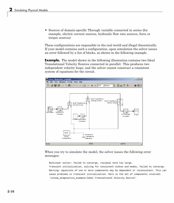
Example. The model shown in the following illustration contains two IdealTranslational Velocity Sources connected in parallel. This produces twoindependent velocity loops, and the solver cannot construct a consistentsystem of equations for the circuit.
When you try to simulate the model, the solver issues the following errormessages:
Nonlinear solver: failed to converge, residual norm too large.
Transient initialization, solving for consistent states and modes, failed to converge.
Warning: equations of one or more components may be dependent or inconsistent. This can
cause problems in transient initialization. Here is the set of components involved:
'vsloop_diagnostics_example/Ideal Translational Velocity Source1'
2-16

Troubleshooting Simulation Errors
'vsloop_diagnostics_example/Ideal Translational Velocity Source'
Initial conditions solve failed to converge.
You can simplify the system by using a single Ideal Translational VelocitySource block, with its control signal supplied by the Sine Wave block. Add theconstant value from the second source to the bias of the sine wave.
Numerical Simulation Issues
• “Dependent Dynamic States” on page 2-17
• “Parameter Discontinuities” on page 2-19
Numerical simulation issues can be either a result of certain circuitconfigurations or of parameter discontinuities.
Dependent Dynamic StatesCertain circuit configurations can result in dependent dynamic states, or theso-called higher-index differential algebraic equations (DAEs). Simscapesolver can handle dependencies among dynamic states that are linear inthe states and independent of time and inputs to the system. For example,capacitors connected in parallel or inductors connected in series will not causeany problems. Other circuit configurations with dependent dynamic states,in certain cases, may slow down the simulation or lead to an error when thesolver fails to initialize.
In electrical circuits, common examples that can cause this behavior includevoltage sources connected in parallel with capacitors, inductors connected inseries with current sources, and so on. To address this issue, the Capacitorand Inductor blocks include parasitic terms (parallel conductance and seriesresistance). For other blocks that do not contain these parasitic terms, youmight need to introduce your own parasitic conductance or resistance intothe circuit. For more information on best modeling practices, as well as fortroubleshooting suggestions, see “Avoiding Numerical Simulation Issues”on page 1-38.
Examples in other domains include direct connections between a velocitysource and a mass, a force source and a spring, a pressure source and a
2-17

2 Simulating Physical Models
hydraulic accumulator, or a flow rate source and a fluid inertia. If youencounter this error, try to either simplify the circuit or include additionalblocks, such as spring-damper combinations or constant orifices, to avoid thedirect connection that results in dependent states.
Example. The model shown in the following illustration contains an IdealTranslational Velocity Source directly connected to a Mass.
When you try to simulate the model, the solver issues the following errormessages:
Nonlinear solver: failed to converge, residual norm too large.
Transient initialization, solving for consistent states and modes, failed to converge.
Warning: problems possible for transient initialization, as well as stepsize control
for transient solve, due to equations of one or more components:
'mech_model1/Mechanical Translational Reference'
'mech_model1//Ideal Translational Velocity Source'
'mech_model1/Mass'
Initial conditions solve failed to converge.
2-18

Troubleshooting Simulation Errors
You can try adding a very stiff spring between the velocity source and themass. To avoid the possibility of high-frequency oscillations introduced by thespring, connect it in parallel with a damper with a high damping coefficient.
Parameter DiscontinuitiesNonlinear parameters, dependent on time or other variables, may also leadto numerical simulation issues as a result of parameter discontinuity. Theseissues usually manifest themselves at the transient initialization stage (see“Transient Simulation Issues” on page 2-20).
Initial Conditions Solve FailureThe initial conditions solve, which solves for all system variables (with initialconditions specified on some system variables), may fail. This has severalpossible causes:
• System configuration error. In this case, the Simulation Diagnosticswindow usually contains additional, more specific, error messages, suchas a missing reference node, or a warning about the component equations,followed by a list of components involved. See “System ConfigurationErrors” on page 2-14 for more information.
2-19

2 Simulating Physical Models
• Dependent dynamic state. In this case, the Simulation Diagnosticswindow also may contain additional, more specific, error messages,such as a warning about the component equations, followed by a list ofcomponents involved. See “Dependent Dynamic States” on page 2-17 formore information.
• The constraint residual tolerance may be too tight to produce a consistentsolution to the algebraic constraints at the beginning of simulation. Youcan try to increase the Constraint Residual Tolerance parameter value(that is, relax the tolerance) in the Solver Configuration block.
If the Simulation Diagnostics window has other, more specific, errormessages, address them first and try rerunning the simulation. See also“Troubleshooting Tips and Techniques” on page 2-13.
Transient Simulation Issues
• “Transient Initialization Not Converging” on page 2-20
• “Step-Size-Related Errors” on page 2-21
Transient initialization happens at the beginning of simulation (aftercomputing the initial conditions) or after a subsequent event, such as adiscontinuity (for example, when a hard stop hits the stop). It is performedby fixing all dynamic variables and solving for algebraic variables andderivatives of dynamic variables. The goal of transient initialization is toprovide a consistent set of initial conditions for the next transient solve step.
Transient Initialization Not ConvergingError messages stating that transient initialization failed to converge, or thata set of consistent initial conditions could not be generated, indicate transientinitialization issues. They can be a result of parameter discontinuity.Review your model to find the possible sources of discontinuity. See also“Troubleshooting Tips and Techniques” on page 2-13.
You can also try to decrease the Constraint Residual Tolerance parametervalue (that is, tighten the tolerance) in the Solver Configuration block.
2-20

Troubleshooting Simulation Errors
Step-Size-Related ErrorsA typical step-size-related error message may state that the system is unableto reduce the step size without violating the minimum step size for a certainnumber of consecutive times. This error message indicates numericaldifficulties in solving the Differential Algebraic Equations (DAEs) for themodel. This might be caused by dependent dynamic states (higher-indexDAEs) or by the high stiffness of the system. You can try the following:
• Tighten the solver tolerance (decrease the Relative Tolerance parametervalue in the Configuration Parameters dialog box)
• Specify a value, other than auto, for the Absolute Tolerance parameterin the Configuration Parameters dialog box. Experiment with thisparameter value.
• Tighten the residual tolerance (decrease the Constraint ResidualTolerance parameter value in the Solver Configuration block)
• Increase the value of the Number of consecutive min step sizeviolations allowed parameter in the Configuration Parameters dialog box(set it to a value greater than the number of consecutive step size violationsgiven in the error message)
• Review the model configuration and try to simplify the circuit, or add smallparasitic terms to your circuit to avoid dependent dynamic states. For moreinformation, see “Numerical Simulation Issues” on page 2-17.
2-21

2 Simulating Physical Models
Finding an Operating Point
In this section...
“What Is an Operating Point?” on page 2-22
“How to Find Operating Points” on page 2-23
“Finding Operating Points with Simscape, Simulink, and Related Products”on page 2-24
What Is an Operating Point?An operating point of a system is a dynamic configuration that satisfies designand use requirements called operating specifications. You can express suchoperating specifications as requirements on the system state x and inputs u.It is not always possible to find a dynamic state that satisfies all operatingconditions. Also, a system might have multiple operating points satisfyingthe same requirements.
Operating points are essential for designing and implementing systemcontrollers. You can optimize a system at an operating point for performance,stability, safety, and reliability.
The most important and common type of operating point is a steady state,where some or all of the system dynamic variables are constant.
Using Operating Points for LinearizationAn important motive for finding operating points is linearization, whichdetermines the system response to small disturbances at an operating point.Linearization results influence the design of feedback controllers to governdynamic behavior near the operating point. A full linearization analysisrequires one or more system outputs, y, in addition to inputs.
See “Linearizing at an Operating Point” on page 2-28.
ExampleA pilot flying an aircraft wants to find, for a given environment, a state of theaircraft engine and control surfaces that produces level, constant-velocity, and
2-22

Finding an Operating Point
constant-altitude flight relative to the ground. The requirements of "level,""constant velocity," "constant altitude," and "relative to the ground" constituteoperating specifications. This operating point is a steady state of the aircraftvelocity, altitude, and orientation in space.
How to Find Operating PointsYou can provide predefined state and input vectors, x0 and u0, to specifyan operating point. If you do not know an operating point in advance, youhave two methods of identifying an operating point that satisfies operatingspecifications.
• “Time-Based Search” on page 2-23: Observing the actual or simulatedbehavior of the system in time is more general, but less precise, and usuallyrequires a trial-and-error process to find a precise operating point.
• “State-Based Search” on page 2-23: If you know the system dynamics, youcan solve for steady states, at least in principle.
Time-Based SearchYou can sometimes find operating points and steady states by trial and errorwhile operating or simulating over some length of time and varying thesystem parameters, inputs, and initial conditions. In such a time-basedapproach, you isolate and study instants or intervals of time when a systemsatisfies the operating specifications. The system state and inputs underthose conditions constitute the operating point, which you can also specifyby an operating or simulation time.
State-Based SearchThe alternative to trial-and-error searching for steady states is trimming.In this state-based approach, you bypass time-based simulation and findsolutions for inputs, outputs, states, and state derivatives satisfying anoperating specification. Trimming specifies inputs and part of a state andsolves the system dynamics for the rest of the state. The resulting full stateand input vectors, x0 and u0, constitute the operating point.
There is no general guarantee that such solutions, x0, exist for given operatingspecifications and inputs, u0.
2-23

2 Simulating Physical Models
Checking Discrete System StatesAn operating point includes the state of discrete system variables thatchange in a discontinuous way. In general, you cannot find these states bysmall, continuous changes of system variables. Such states usually requiresystematic exploration of the discrete variables over the full range of theirpossible values.
Finding Operating Points with Simscape, Simulink,and Related ProductsYou have a number of ways to find an operating point in a Simscape model.You can impose operating specifications and isolate operating points usingSimscape and Simulink features and, in some cases, with such relatedproducts as Simulink® Control Design™ and Control System Toolbox™software. The full state vector of your model contains:
• Simulink components, which can be continuous or discrete.
• Simscape components, which are continuous.
Tip Whichever method that you choose to find an operating point, if you wantto use it for linearization, you must save the operating point information inthe form of a simulation time t0, a state vector x0, and an input vector u0,or an operating point object.
Simulating in Time to Search for an Operating PointOne way to identify operating points is to simulate your model and inspect itsstate x and output y as a time series.
1 In your Simscape model, set up sensor outputs for whatever block outputsyou want to observe.
2 Connect Scope blocks, To Workspace blocks, or both, to your Simscapeblock outputs to observe and record simulation behavior.
3 In the Data Import/Export pane of your model Configuration Parameterssettings, select the Time, States, and Output check boxes to record thissimulation information in your workspace.
2-24

Finding an Operating Point
Using the Simscape Steady-State SolverMost commonly, the operating point that you want is a steady state. You havea precise method for identifying steady states with the Simscape steady-statesolver, which allows you to isolate steady states more exactly than you canwith ordinary simulation. It is particularly recommended for isolating steadystates of a strongly nonlinear character. You can search for multiple steadystates with the steady-state solver by varying the model inputs, parameters,and initial conditions.
The Simscape steady-state solver initializes the system and inputs first,then determines a steady state. In general, the system does not remain inthis initial steady state x(t=0) = x0 during simulation, because the systeminputs u change independently, and the system has to respond by changingits state x(t).
To implement the steady-state solver:
1 In each, some, or all of the physical networks in your Simscape model,open the Solver Configuration block.
2 In each block dialog box, select the Start simulation from steady statecheck box.
3 In the model Configuration Parameters settings, on the DataImport/Export pane, select the States check box to record the time seriesof x values in your workspace.
If you also have input signals u in the model, you can capture those inputsby connecting To Workspace blocks to the input Simulink signal lines.
4 Close these dialog boxes and start simulation.
The first vector of values x(t=0) that you capture during simulation reflectsthe steady state x0 that the Simscape solver identified.
2-25

2 Simulating Physical Models
Using Simulink Control Design Techniques
Note The techniques described in this section require the Simulink ControlDesign product. You must use the features of this product on the Simulinklines in your model, not directly on Simscape physical network lines or blocks.
The following methods are state-based, allowing you to impose operatingspecifications, and work well for simple to moderately complex Simscapemodels. The MathWorks™ does not recommend these methods for highlycomplex Simscape models.
To find operating points, use the operspec and findop functions, customizingwhere necessary. Create an operating specification object with operspec,then compute an operating point object with findop. The findop functionattempts to find an operating point that satisfies the operating specificationsand reports on its success or failure. If the search is successful, find_opreturns state values satisfying the operating specifications.
You have several choices for operating specifications for the components ofthe state vector.
AssumedOperatingCondition
Operating Specification
Default Request that all state component derivatives be zero.This is a steady-state for the whole model, not just aSimscape network within the model.
Nondefault Request any value you want independently for eachstate component.
Nondefault Request that a particular state component derivativebe zero.This is a steady-state condition for that statecomponent.
2-26

Finding an Operating Point
Additional Simulink Control Design Methods. Instead of the commandline interface, you can use the associated graphical user interface, throughthe model menu bar: Tools > Control Design > Linear Analysis. For moredetails on the use of operating point specification objects, related functions,and the graphical interface, see the Simulink Control Design documentation.
Using Sources to Find Operating Points Not RecommendedYou can impose an operating specification on part of a Simscape model byinserting source blocks from the Simscape Foundation Library. These imposespecified values of system variables in parts of the model. You can simulateand save the state vector.
However, you cannot obtain an operating point for the original system(without the source blocks) by saving the state values from the model andthen removing the source blocks. In general, the number, order, and identityof state components change after adding and removing Simscape blocks ina model.
Simulink trim Function Not Supported with Simscape ModelsThe Simulink trim function is not supported for models containing Simscapecomponents.
2-27
2 Simulating Physical Models
Linearizing at an Operating Point
In this section...
“What Is Linearization?” on page 2-28
“How to Linearize a Model” on page 2-30
“Linearizing a Model with Simscape, Simulink, and Related Products” onpage 2-30
“References” on page 2-34
What Is Linearization?Determining the response of a system to small perturbations at an operatingpoint is a critical step in system and controller design. Once you find anoperating point, you can linearize the model about that operating point toexplore the response and stability of the system. To find an operating point ina Simscape model, see “Finding an Operating Point” on page 2-22.
Choosing a Good Operating Point for LinearizationAlthough steady-state and other operating points (state x0 and inputs u0)might exist for your model, that is no guarantee that such operating points aresuitable for linearization. The critical question is: how good is the linearizedapproximation compared to the exact system dynamics?
• When perturbed slightly, a problematic operating point might exhibitstrong asymmetries, with strongly nonlinear behavior when perturbed incertain ways and smoother behavior in other ways.
• Small perturbations might change discrete states in a large, discontinuousway that violates the linear approximation.
Operating points with a strongly nonlinear or discontinuous character are notsuitable for linearization. You should analyze them in full simulation andperturb the system by varying its inputs, parameters, and initial conditions.
2-28

Linearizing at an Operating Point
Tip A reliable way to check for such an unsuitable operating point is tolinearize at several nearby operating points. If the results differ greatly, theoperating point is strongly nonlinear.
What Is Linear Response?Near an operating point, you can express the system state x, inputs u, andoutputs y relative to that operating point in terms of x – x0, u – u0, and y –y0. For convenience, shift the vectors by subtracting the operating point:x – x0 → x, etc.
If the system dynamics does not explicitly depend on time and the operatingpoint is a steady state, the system response to state and input perturbationsnear the steady state is approximately governed by a linear time-invariant(LTI) state space model:
dx/dt = A·x + B·u
y = C·x + D·u.
The matrices A, B, C, D have components and structures that are independentof the simulation time. A system is stable to changes in state at an operatingpoint if the eigenvalues of A are negative.
If the operating point is not a steady state or the system dynamics dependsexplicitly on time, the linearized dynamics near the operating point is morecomplicated. The matrices A, B, C, D are not constant and depend on thesimulation time t0 , as well as the operating point x0 and u0 [1].
Tip While you can linearize a closed system with no inputs or outputs andobtain a nonzero A matrix, obtaining a nontrivial linearized input-outputmodel requires at least one input component in u and one output componentin y.
2-29

2 Simulating Physical Models
ExampleA pilot is flying, or simulating, an aircraft in level, constant-velocity, andconstant-altitude flight relative to the ground, with a known environment. Acrucial question for the aircraft pilot and designers is: will the aircraft returnto the steady state if perturbed from it by a disturbance, such as a windgust — in other words, is this steady state stable? If the operating point isunstable, the aircraft trajectory can diverge from the steady state, requiringhuman or automatic intervention to maintain steady flight.
How to Linearize a ModelOnce you know an operating point, you have three practical methods forinvestigating the system response to small disturbances.
Full Simulation- or Operation-Based PerturbationsYou can experiment with the system or a system simulation by makingrepeated, different, and slight changes to the system parameters, inputs,and initial conditions, while operating at a steady state. This methodrequires costly trial and error and generates uncontrolled and impreciseapproximations.
Analytic Approximations to Known State DynamicsIf you know the system state dynamics and an operating point x0 and u0 inanalytic form, you can apply standard approximation techniques to derive ananalytic form for the A, B, C, D matrices.
Numerical Approximations to Known State DynamicsIf you have a controlled numerical approximation to your system statedynamics and operating point, you can apply standard computationaltechniques to generate numerical approximations to the A, B, C, D matrices.
Linearizing a Model with Simscape, Simulink, andRelated ProductsUse the following methods to create numerical linearized state-space modelsfrom a model containing Simscape components.
2-30

Linearizing at an Operating Point
Independent Versus Dependent StatesAn important difference from normal Simulink models is that the states in aphysical network are not independent in general, because some states havedependencies on other states through constraints.
• The independent states are a subset of system variables and consist ofSimscape dynamic variables and Simulink states.
• The dependent states consist of Simscape algebraic variables anddependent (constrained) dynamic variables.
For more information on Simscape dynamic and algebraic variables, see “HowSimscape Simulation Works” on page 2-2.
The only components of the A, B, C, D matrices that can be nonzero are thosecorresponding to independent states.
• The A matrix, of size n_states by n_states, is all zeros except fora submatrix of size n_ind by n_ind, where n_ind is the number ofindependent states.
• The B matrix, of size n_states by n_inputs, is all zeros except for asubmatrix of size n_ind by n_inputs.
• The C matrix, of size n_outputs by n_states, is all zeros except for asubmatrix of size n_outputs by n_ind.
• The D matrix, of size n_outputs by n_inputs, can be nonzeros everywhere.
Obtaining the Independent Subset of States. A complete linearizedsolution uses only an independent subset of the system states. From thematrices A, B, C, D, you can obtain a minimal input-output linearized modelwith the minreal and sminreal functions from Control System Toolboxsoftware.
Linearizing with the Simulink linmod and dlinmod FunctionsThe Simulink functions linmod and dlinmod provide a way of linearizinga Simscape model. There are several ways that you can use linmod anddlinmod, and the linearization results differ depending on the method chosen.To use these functions, you do not have to open the model, just have the modelfile on your MATLAB path.
2-31

2 Simulating Physical Models
For more information about Simulink linearization, see “Linearizing Models”in the Simulink documentation.
Note If your model has continuous states, use linmod. (Continuous statesare the Simscape default.) If your model has mixed continuous and discretestates, or purely discrete states, use dlinmod.
Linearizing a model with the local solver enabled (in the Solver Configurationblock) is not supported.
Linearizing with Default State and Input. You can call linmod withoutspecifying state or input. Enter linmod('modelname') at the command line.
With this form of linmod, Simulink linearization solves for consistent initialconditions in the same way it does on the first step of any simulation. Inparticular, any initial conditions, such as initial offset from equilibrium for aspring, are set as if the simulation were starting from the initial time.
linmod allows you to change the time of externally specified signals (but notthe internal system dynamics) from the default. For this and more details, seethe function reference page.
Linearizing with the Steady-State Solver at an Initial Steady State.If you have previously used the Simscape steady-state solver to find anoperating point, you can linearize at that operating point:
1 Open one or more Solver Configuration blocks in your model.
2 Select the Start simulation from steady state check box for the physicalnetworks that you want to linearize.
3 Close the Solver Configuration dialog boxes and save the modified model.
4 Enter linmod('modelname') at the command line.
linmod linearizes at the first step of simulation. In this case, the initial stateis also an operating point, a steady state.
2-32
Linearizing at an Operating Point
For more about setting up the steady-state solver, see the Solver Configurationblock reference page. For more details on its use, see “Using the SimscapeSteady-State Solver” on page 2-25.
Linearizing with Specified State and Input — Ensuring Consistencyof States. You can call linmod and specify state and input. Enterlinmod('modelname',x0,u0) at the command line. The extra argumentsspecify, respectively, the steady state x0 and inputs u0 for linearizingthe simulation. When you specify a state to linmod, ensure that it isself-consistent, within solver tolerance.
With this form of linmod, Simulink linearization does not solve for initialconditions. Because not all states in the model have to be independent, it ispossible, though erroneous, to provide linmod with an inconsistent state tolinearize about.
If you specify a state that is not self-consistent (within solver tolerance), theSimscape solver issues a warning at the command line when you attemptlinearization. The Simscape solver then attempts to make the specified x0consistent by changing some of its components, possibly by large amounts.
Tip You most easily ensure a self-consistent state by taking the state fromsome simulated time. For example, by selecting the States check box on theData Import/Export pane of the model Configuration Parameters dialogbox, you can capture a time series of state values in a simulation run.
Linearizing with Simulink Linearization BlocksYou can generate linearized state-space models from your Simscape model byadding a Timed-Based Linearization or Trigger-Based Linearization block tothe model and simulating. These blocks combine time-based simulation up tospecified times or internal trigger points, with state-based linearization atthose times or trigger points.
For complete details about these blocks, see their respective block referencepages.
2-33

2 Simulating Physical Models
Linearizing with Simulink Control Design Software
Note The techniques described in this section require the Simulink ControlDesign product. You must use the features of this product on the Simulinklines in your model, not directly on Simscape physical network lines or blocks.
The following methods require that you start with an operating point objectsaved from trimming the model to an operating specification, as explained in“Using Simulink® Control Design Techniques” on page 2-26.
To linearize a model with an operating point object, use the linearizefunction, customizing where necessary. The resulting state-space objectcontains the matrices A, B, C, D.
Additional Simulink Control Design Methods. Instead of the commandline interface, you can use the associated graphical user interface, throughthe model menu bar: Tools > Control Design > Linear Analysis. For moredetails on linearization, operating points and state-space objects, relatedfunctions, and the graphical interface, see the Simulink Control Designdocumentation.
References
[1] Brogan, W. L., Modern Control Theory, 2nd Ed., Englewood Cliffs, NewJersey, Prentice-Hall, 1985.
[2] The MathWorks, Control System Toolbox User Guide,www.mathworks.com/access/helpdesk/help/toolbox/control/.
2-34

Generating Code
Generating Code
In this section...
“About Code Generation from Simscape Models” on page 2-35
“Related Simulink Code Generation Documentation” on page 2-35
“Reasons for Generating Code” on page 2-36
“Using Code-Related Products and Features” on page 2-36
“How Simscape Code Generation Differs from Simulink” on page 2-37
About Code Generation from Simscape ModelsYou can use Real-Time Workshop® software to generate stand-alone C codefrom your Physical Networks models and enhance simulation speed andportability. Certain features of Simulink software also make use of generatedor external code. This section explains code-related tasks you can performwith your Simscape models.
Code versions of Simscape models typically require fixed-step Simulinksolvers, which are discussed in the Simulink documentation. Some features ofSimscape software are restricted when you translate a model into code. See“How Simscape Code Generation Differs from Simulink” on page 2-37, aswell as “Limitations” on page 2-39.
Note Code generated from Simscape models is intended for rapid prototypingand hardware-in-the-loop applications. It is not intended for use as productioncode in embedded controller applications.
Add-on products based on the Simscape platform also support code generation,with some variations and exceptions described in their respective User’sGuides. Consult those User’s Guides for more information.
Related Simulink Code Generation DocumentationConsult Simulink Acceleration modes, Real-Time Workshop, and xPCTarget™ documentation for general information on code generation.
2-35
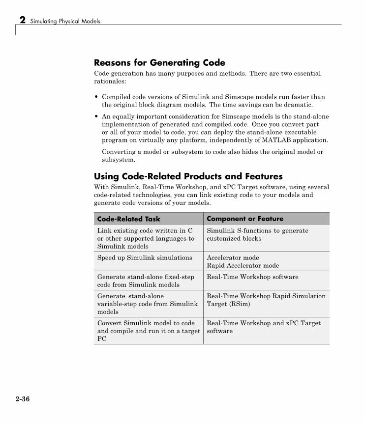
2 Simulating Physical Models
Reasons for Generating CodeCode generation has many purposes and methods. There are two essentialrationales:
• Compiled code versions of Simulink and Simscape models run faster thanthe original block diagram models. The time savings can be dramatic.
• An equally important consideration for Simscape models is the stand-aloneimplementation of generated and compiled code. Once you convert partor all of your model to code, you can deploy the stand-alone executableprogram on virtually any platform, independently of MATLAB application.
Converting a model or subsystem to code also hides the original model orsubsystem.
Using Code-Related Products and FeaturesWith Simulink, Real-Time Workshop, and xPC Target software, using severalcode-related technologies, you can link existing code to your models andgenerate code versions of your models.
Code-Related Task Component or Feature
Link existing code written in Cor other supported languages toSimulink models
Simulink S-functions to generatecustomized blocks
Speed up Simulink simulations Accelerator modeRapid Accelerator mode
Generate stand-alone fixed-stepcode from Simulink models
Real-Time Workshop software
Generate stand-alonevariable-step code from Simulinkmodels
Real-Time Workshop Rapid SimulationTarget (RSim)
Convert Simulink model to codeand compile and run it on a targetPC
Real-Time Workshop and xPC Targetsoftware
2-36

Generating Code
How Simscape Code Generation Differs fromSimulinkIn general, using the code generated from Simscape models is similar to usingcode generated from regular Simulink models. However, there are certaindifferences.
Simscape and Simulink Code Are Generated SeparatelyReal-Time Workshop software generates code from the Simscape blocksseparately from the Simulink blocks in your model. The generated Simscapecode does not pass through model.rtw or the Target Language Compiler. Allthe code generated from a single model resides in the same directory, however.
Compiler Support and Precompiled LibrariesSimscape software and its add-on products provide static runtime librariesprecompiled for compilers supported by Real-Time Workshop software. Theseare the standard UNIX compilers for UNIX operating systems, LCC andMicrosoft® Visual Studio® for 32-bit Windows®, and Microsoft Visual Studiofor 64-bit Windows.
For all other compilers, the static runtime libraries needed by code generatedfrom Simscape models are compiled once per model during the code generationbuild process.
Simscape Code Reuse Is Not SupportedReusable subsystems in Simulink reuse code that is generated once from thesubsystem. You cannot generate reusable code from subsystems containingSimscape blocks.
Tunable Parameters Are Not SupportedA tunable parameter is a Simulink run-time parameter that you can changewhile the simulation is running. Simscape blocks do not support tunableparameters in either simulations or generated code.
2-37

2 Simulating Physical Models
Simscape Run-Time Parameter Inlining Ignores GlobalExceptionsIf you choose to enable parameter inlining for code generated from a Simscapemodel, the software inlines all its run-time parameters. If you choose to makesome of the global Simscape block parameters exceptions to inlining, theexceptions are ignored. You can change global tunable parameters only byregenerating code from the model.
2-38

Limitations
Limitations
In this section...
“Sample Time and Solver Restrictions” on page 2-39
“Algebraic Loops” on page 2-39
“Restricted Simulink Tools” on page 2-40
“Unsupported Simulink Tools” on page 2-42
“Simulink Tools Not Compatible with Simscape Blocks” on page 2-42
“Code Generation” on page 2-42
Sample Time and Solver RestrictionsThe default sample times of Simscape blocks are continuous. You cannotsimulate Simscape blocks with discrete solvers using the default sample times.
If you switch to a local solver in the Solver Configuration block, the associatedstates become discrete. If there are no continuous Simulink or Simscapestates elsewhere in the model, you should use a discrete solver to simulatesuch a model.
You cannot override the sample time of a nonvirtual subsystem containingSimscape blocks.
Algebraic LoopsA Simscape physical network should not exist within a Simulink algebraicloop. This means that you should not directly connect an output of aPS-Simulink Converter block to an input of a Simulink-PS Converter block ofthe same physical network.
For example, the following model contains a direct feedthrough betweenthe PS-Simulink Converter block and the Simulink-PS Converter block(highlighted in magenta). To avoid the algebraic loop, you can insert aTransfer Function block anywhere along the highlighted loop.
2-39
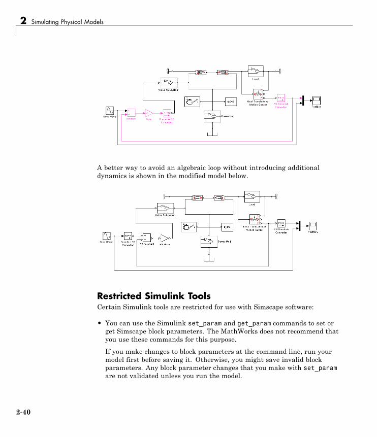
2 Simulating Physical Models
A better way to avoid an algebraic loop without introducing additionaldynamics is shown in the modified model below.
Restricted Simulink ToolsCertain Simulink tools are restricted for use with Simscape software:
• You can use the Simulink set_param and get_param commands to set orget Simscape block parameters. The MathWorks does not recommend thatyou use these commands for this purpose.
If you make changes to block parameters at the command line, run yourmodel first before saving it. Otherwise, you might save invalid blockparameters. Any block parameter changes that you make with set_paramare not validated unless you run the model.
2-40
Limitations
• Enabled subsystems can contain Simscape blocks. Always set the Stateswhen enabling parameter in the Enable dialog to held for the subsystem’sEnable port.
Setting States when enabling to reset is not supported and can leadto fatal simulation errors.
• You can place Simscape blocks within nonvirtual subsystems that supportcontinuous states. Nonvirtual subsystems that support continuous statesinclude Enabled subsystems and Atomic subsystems. However, physicalconnections and physical signals must not cross nonvirtual boundaries.When placing Simscape blocks in a nonvirtual subsystem, make sureto place all blocks belonging to a given Physical Network in the samenonvirtual subsystem.
• Simulink configurable subsystems work with Simscape blocks only if all ofthe block choices have consistent port signatures.
• For Iterator, Function-Call, Triggered, and While Iterator nonvirtualsubsystems cannot contain Simscape blocks.
• An atomic subsystem with a user-specified (noninherited) sample timecannot contain Simscape blocks.
• You can use the Simulink Save As command only to rename Simscapemodels within the current version. Saving in a previous version format isnot supported for models containing Simscape blocks.
• Linearization with the Simulink linmod function or with equivalentSimulink Control Design functions and graphical interfaces is notsupported with Simscape models if you use local solvers.
• Model referencing is supported, with some restrictions:
- All Physical connection lines must be contained within the referencedmodel. Such lines cannot cross the boundary of the referenced modelsubsystem in the referencing model.
- The referencing model and the referenced model must use the samesolver.
For further information, consult the Simulink documentation onreferencing models.
2-41

2 Simulating Physical Models
Unsupported Simulink ToolsCertain Simulink tools and features do not work with Simscape software:
• The Simulink Profiler tool does not work with Simscape models.
• Physical signals and physical connection lines between conserving ports aredifferent from Simulink signals. Therefore, the Signal and Scope Managertool and the signal label functionality are not supported.
Simulink Tools Not Compatible with Simscape BlocksSome Simulink tools and features do not work with Simscape blocks:
• Execution order tags do not appear on Simscape blocks.
• Simscape blocks do not invoke user-defined callbacks.
• You cannot set breakpoints on Simscape blocks.
• Reusable subsystems cannot contain Simscape blocks.
• You cannot use the Simulink Fixed-Point Tool with Simscape blocks.
• The Report Generator reports Simscape block properties incompletely.
Code GenerationCode generation is supported for Simscape physical modeling software and itsfamily of add-on products. However, there are restrictions on code generatedfrom Simscape models.
• Code reuse is not supported.
• C++ code generation is not supported.
• Tunable parameters are not supported.
• Run-time parameter inlining ignores global exceptions.
• Simulation of Simscape models on fixed-point processors is not supported.
• Block diagnostics in error messages are not supported. This means thatif you get an error message from simulating generated code, it does notcontain a list of blocks involved.
• Conversion of models or subsystems containing Simscape blocks toS-functions is not supported.
2-42

Limitations
• Simulation-in-the-loop (SIL) is not supported.
• Code generation respects the Linear Algebra setting in the SolverConfiguration block, but only when you choose the local solver option.Otherwise, code generation uses full linear algebra.
“Generating Code” on page 2-35 describes Simscape code generation features.“Restricted Simulink Tools” on page 2-40 describes limitations on modelreferencing.
There are variations and exceptions as well in the code generation features ofthe add-on products based on Simscape platform. For details, see the User’sGuides for individual add-on products.
Code Generation and Fixed-Step SolversMost code generation options for Simscape models require the use of fixed-stepSimulink solvers. This table summarizes the available solver choices,depending on how you generate code.
Code Generation Option Solver Choices
Accelerator modeRapid Accelerator mode
Variable-step or fixed-step
Real-Time Workshop software: RSimTarget*
Variable-step or fixed-step
Real-Time Workshop software: Targetsother than RSim
Fixed-step only
* For the RSim Target, Simscape software supports only the Simulinksolver module. In the model Configuration Parameters dialog box, see theReal-Time Workshop: RSim Target: Solver selection menu. The defaultis automatic selection, which might fail to choose the Simulink solver module.
2-43

2 Simulating Physical Models
2-44

3
Logging Simulation Data
• “About Simulation Data Logging” on page 3-2
• “How to Log Simulation Data” on page 3-3
• “Data Logging Example” on page 3-6

3 Logging Simulation Data
About Simulation Data Logging
In this section...
“Suggested Workflows” on page 3-2
“Limitations” on page 3-2
Suggested WorkflowsYou can log simulation data to the workspace for debugging and verification.Data logging lets you analyze how internal block variables change with timeduring simulation. For example, you may want to see that the pressure in ahydraulic cylinder is above some minimum value, or compare it against thepump pressure. If you log simulation data to the workspace, you can laterquery, plot, and analyze it without rerunning the simulation.
Simulation data logging can also replace connecting sensors and scopes totrack simulation data. These blocks increase the model complexity and slowdown simulation. The “Data Logging Example” on page 3-6 shows how youcan log and plot simulation data instead of adding sensors to your model. Italso shows how you can print the complete logging tree for a model, and plotsimulation results for a selected variable.
For additional information, see the reference pages for the classessimscape.logging.Node, simscape.logging.Series, and their associatedmethods.
LimitationsSimulation data logging is not supported for:
• Model reference
• Generated code
• Accelerator mode
• Rapid Accelerator mode
3-2
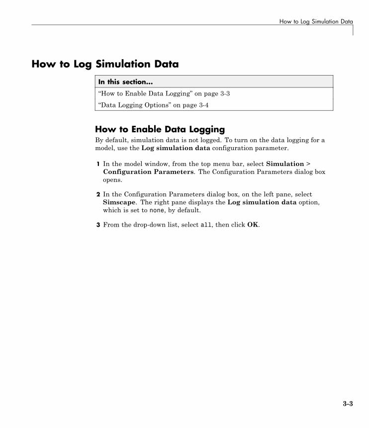
How to Log Simulation Data
How to Log Simulation Data
In this section...
“How to Enable Data Logging” on page 3-3
“Data Logging Options” on page 3-4
How to Enable Data LoggingBy default, simulation data is not logged. To turn on the data logging for amodel, use the Log simulation data configuration parameter.
1 In the model window, from the top menu bar, select Simulation >Configuration Parameters. The Configuration Parameters dialog boxopens.
2 In the Configuration Parameters dialog box, on the left pane, selectSimscape. The right pane displays the Log simulation data option,which is set to none, by default.
3 From the drop-down list, select all, then click OK.
3-3

3 Logging Simulation Data
4 Simulate the model. This creates a workspace variable named simlog (asspecified by the Workspace variable name parameter), which containsthe simulation data.
For information on how to access and use the data stored in this variable, see“Data Logging Example” on page 3-6.
Data Logging OptionsWhen you set the Log simulation data configuration parameter to all,other options in the Data Logging group box become available.
• Workspace variable name — Specifies the name of the workspacevariable that stores the simulation data. Subsequent simulations overwritethe data in the simulation log variable. If you want to compare data from
3-4
How to Log Simulation Data
two models or two simulation runs, use different names for the respectivelog variables. The default variable name is simlog.
• Limit data points — Saving data to the workspace can slow down thesimulation and consume memory. Use this checkbox in conjunction withthe Data history (last N steps) parameter to limit the number of datapoints saved. The checkbox is selected by default. If you clear it, thesimulation log variable contains the data points for the whole simulation,at the price of slower simulation speed and heavier memory consumption.
• Data history (last N steps)— Specify the number of simulation steps tolimit the number of data points output to the workspace. The simulationlog variable contains the data points corresponding to the last N steps of thesimulation, where N is the value that you specify for theData history (lastN steps) parameter. You have to select the Limit data points checkboxto make this parameter available. The default value logs simulation datafor the last 5000 steps. You can specify any other positive integer number.If the simulation contains fewer steps than the number specified, thesimulation log variable contains the data points for the whole simulation.
After changing your data logging preferences, rerun the simulation togenerate a new data log.
3-5

3 Logging Simulation Data
Data Logging ExampleThe model shown represents a permanent magnet DC motor.
This model is very similar to the Permanent Magnet DC Motor demo, but,unlike the demo model, it does not include the Ideal Rotational MotionSensor and the Current Sensor blocks, along with the respective PS-SimulinkConverter blocks and scopes. For a detailed description of the PermanentMagnet DC Motor demo, see “Working with a Simscape Demo Model” in theSimscape Getting Started Guide.
This example shows how you can log and plot simulation data instead ofadding sensors to your model.
1 Build the model, as shown in the preceding illustration.
2 To enable data logging, open the Configuration Parameters dialog box,in the left pane, select Simscape, then set the Log simulation dataparameter to all and click OK.
3-6

Data Logging Example
3 Simulate the model. This creates a workspace variable named simlog (asspecified by the Workspace variable name parameter), which containsthe simulation data.
4 The simlog variable has the same hierarchy as the model. To see the wholevariable structure, at the command prompt, type:
simlog.print
This command prints the whole data tree.
dc_motor1+-Electrical_Reference2| +-V| | +-v| +-i
3-7

3 Logging Simulation Data
+-Friction_Mr| +-C| | +-w| +-R| | +-w| +-t| +-w+-L| +-i| +-i_L| +-n| | +-v| +-p| | +-v| +-v+-Load_Torque| +-C| | +-w| +-R| | +-w| +-S| +-t| +-w+-Mechanical_Rotational_Reference| +-W| | +-w| +-t+-Mechanical_Rotational_Reference1| +-W| | +-w| +-t+-Motor_Inertia_J| +-I| | +-w| +-t+-Rotational_Electromechanical_Converter| +-C| | +-w| +-R| | +-w
3-8

Data Logging Example
| +-i| +-n| | +-v| +-p| | +-v| +-t| +-v| +-w+-Rotor_Resistance_R| +-i| +-n| | +-v| +-p| | +-v| +-v+-Simulink_PS_Converter+-x1_5V
+-i+-n| +-v+-p| +-v+-v
5 Every node that represents an Across, Through, or internal block variablecontains series data. To get to the series, you have to specify the completepath to it through the tree, starting with the top-level variable name. Forexample, to get a handle on the series representing the angular velocity ofthe motor, type:
s1 = simlog.Rotational_Electromechanical_Converter.R.w.series;
6 To see how the motor speed changes with time, type:
plot(s1.time, s1.values)
This plots the motor speed in default units (radian/s).
3-9

3 Logging Simulation Data
7 To get a plot in revolutions per minute, type:
plot(s1.time, s1.values('rpm'))
3-10

Data Logging Example
8 Compare this figure to the RPM scope display in the Permanent MagnetDC Motor demo. The results are exactly the same.
9 To plot the current through the motor, type:
s2 = simlog.Rotational_Electromechanical_Converter.i.series;plot(s2.time, s2.values)
3-11
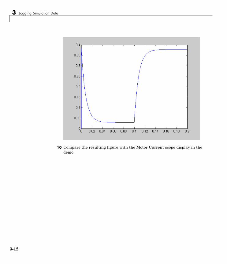
3 Logging Simulation Data
10 Compare the resulting figure with the Motor Current scope display in thedemo.
3-12

4
Working with PhysicalUnits
• “Overview” on page 4-2
• “Unit Definitions” on page 4-4
• “Specifying Units in Block Dialogs” on page 4-9
• “Thermal Unit Conversions” on page 4-11
• “Angular Units” on page 4-14

4 Working with Physical Units
OverviewUnlike Simulink signals, which are essentially unitless, physical signalscan have units associated with them. You specify the units along with theparameter values in the block dialogs, and Simscape unit manager performsthe necessary unit conversion operations when solving a physical network.Simscape blocks support standard measurement systems. The default blockunits are meter-kilogram-second or MKS (SI).
Simscape software comes with a library of standard units, and you can defineadditional units as needed (see “Unit Definitions” on page 4-4). You can usethese units in your block diagrams:
• To specify the units of an input physical signal, type a unit name, or amathematical expression with unit names, in the Input signal unit fieldof the Simulink-PS Converter block dialog. You can also select a unitfrom a drop-down list, which is prepopulated with some common inputunits. Signal units that you specify in a Simulink-PS Converter block mustmatch the input type expected by the Simscape block connected to it. Forexample, when you provide the input signal for an Ideal Angular VelocitySource block, specify angular velocity units, such as rad/s or rpm, in theSimulink-PS Converter block, or leave it unitless. If you leave the blockunitless, with the Input signal unit parameter set to 1, then the physicalsignal units are inferred from the destination block.
• Simscape block dialogs have drop-down combo boxes of units next to aparameter value, letting you either select a unit from the drop-down list, ortype a unit name (or a mathematical expression with unit names) directlyinto the box. These drop-down lists are automatically populated by thoseunits that are commensurate with the unit of the parameter, based on thecurrent list of unit definitions. For example, if a parameter is specified, bydefault, with the units of meters per second, m/s, the drop-down list of unitscontains commensurate units, such as mm/s, in/s, fps (feet per second),fpm (feet per minute), and so on, including any other linear velocity unitscurrently defined in your unit registry.
• To specify the units of an output physical signal, type a unit name, or amathematical expression with unit names, in the Output signal unitfield of the PS-Simulink Converter block dialog. You can also select a unitfrom a drop-down list, which is prepopulated with some common outputunits. The system compares the units you specified with the actual units
4-2

Overview
of the input physical signal coming into the converter block and applies again equal to the conversion factor before outputting the Simulink signal.The default value is 1, which means that the unit is not specified. If youdo not specify a unit, or if the unit matches the actual units of the inputphysical signal, no gain is applied.
For more information, see “Specifying Units in Block Dialogs” on page 4-9.
4-3

4 Working with Physical Units
Unit DefinitionsSimscape unit names are defined in the pm_units.m file, which isshipped with the product. You can open this file to see how thephysical units are defined in the product, and also as an examplewhen adding your own units. This file is located in the directorymatlabroot\toolbox\physmod\unit_manager\unit_manager.
Default registered units and their abbreviations are listed in the followingtable. Use the pm_getunits command to get an up-to-date list of unitscurrently defined in your unit registry. Use the pm_adddimension andpm_addunit commands to define additional units.
Physical Unit Abbreviations Defined by Default in the Simscape UnitRegistry
Quantity Abbreviation Unit
Amount of substance mol Mole
Angle rad
deg
rev
Radian
Degree
Revolution
Angular velocity rpm
Hz
Revolutions/minute
Revolutions/second
Capacitance F
pF
nF
uF
Farad
Picofarad
Nanofarad
Microfarad
Charge c Coulomb
Conductance S
nS
uS
mS
Siemens
Nanosiemens
Microsiemens
Millisiemens
4-4

Unit Definitions
Physical Unit Abbreviations Defined by Default in the Simscape UnitRegistry (Continued)
Quantity Abbreviation Unit
Current A
pA
nA
uA
mA
kA
Ampere
Picoampere
Nanoampere
Microampere
Milliampere
Kiloampere
Energy J
Btu
eV
Joule
British thermal unit
Electronvolt
Flow rate lpm
gpm
Liter/minute
Gallon/minute
Force N
dyn
lbf
mN
Newton
Dyne
Pound-force
Millinewton
Inductance H
uH
mH
Henry
Microhenry
Millihenry
4-5

4 Working with Physical Units
Physical Unit Abbreviations Defined by Default in the Simscape UnitRegistry (Continued)
Quantity Abbreviation Unit
Length m
cm
mm
km
um
in
ft
mi
yd
Meter
Centimeter
Millimeter
Kilometer
Micrometer
Inch
Foot
Mile
Yard
Magnetic flux Wb Weber
Magnetic flux density T
G
Tesla
Gauss
Mass kg
g
mg
lbm
oz
slug
Kilogram
Gram
Milligram
Pound mass
Ounce
Slug
Pressure Pa
bar
atm
psi
Pascal
Bar
Atmosphere
Pound/inch^2
Power W
HP
Watt
Horsepower
4-6

Unit Definitions
Physical Unit Abbreviations Defined by Default in the Simscape UnitRegistry (Continued)
Quantity Abbreviation Unit
Resistance Ohm
kOhm
MOhm
GOhm
Ohm
Kiloohm
Megaohm
Gigaohm
Temperature K
C
Fh
R
Kelvin
Celsius
Fahrenheit
Rankine
Time s
min
hr
ms
us
ns
Second
Minute
Hour
Millisecond
Microsecond
Nanosecond
Velocity mph
fpm
fps
Miles/hour
Feet/minute
Feet/second
Viscosity absolute Poise
cP
reyn
Poise
Centipoise
Reyn
Viscosity kinematic St
cSt
Newt
Stokes
Centistokes
Newt
4-7

4 Working with Physical Units
Physical Unit Abbreviations Defined by Default in the Simscape UnitRegistry (Continued)
Quantity Abbreviation Unit
Volume l
gal
Liter
Gallon
Voltage V
mV
kV
Volt
Millivolt
Kilovolt
Note This table lists the unit abbreviations defined in the product. Seethe following section, “Specifying Units in Block Dialogs” on page 4-9,for information on how to use the abbreviations above, or mathematicalexpressions with these abbreviations, to specify units for the parametervalues in the block dialogs.
4-8

Specifying Units in Block Dialogs
Specifying Units in Block DialogsSimscape block dialogs have drop-down combo boxes for units next to aparameter value. For example, in the Constant Volume Chamber block,the drop-down list for the Chamber volume parameter contains l, gal,in^3, ft^3, mm^3, cm^3, m^3, and km^3, and the drop-down list for the Initialpressure parameter contains Pa, bar, psi, and atm.
You can either select a unit from the drop-down list, or type a commensurateunit name (or a mathematical expression with unit names) directly into theunit combo box of the block dialog. You can use the abbreviations for theunits defined in your registry, or any valid mathematical expressions withthese abbreviations. For example, you can specify torque in newton-meters(N*m) or pound-feet (lbf*ft). To specify velocity, you can use one of thedefined unit abbreviations (mph, fpm, fps), or an expression based on anycombination of the defined units of length and time, such as meters/second(m/s), millimeters/second (mm/s), inches/minute (in/min), and so on.
Note Affine units (such as Celsius or Fahrenheit) are not allowed in unitexpressions. For more information, see “About Affine Units” on page 4-11.
The following operators are supported in the unit mathematical expressions:
* Multiplication
/ Division
^ Power
+, - Plus, minus — for exponents only
() Brackets to specify evaluation order
Metric unit prefixes, such as kilo, milli, or micro, are not supported. Forexample, if you want to use milliliter as a unit of volume, you have to addit to the unit registry:
pm_addunit('ml', 0.001, 'l');
4-9

4 Working with Physical Units
The drop-down lists next to parameter names are automatically populatedby those units that are commensurate with the unit of the parameter. If youspecify the units by typing, it is your responsibility to enter units that arecommensurate with the unit of the parameter. The unit manager performserror checking when you click Apply or OK in the block dialog box, and issuesan error if you type an incorrect unit.
In the Simulink-PS Converter and the PS-Simulink Converter block dialogs,the drop-down lists are prepopulated with some common input and outputunits, and it is your responsibility to select or type a unit expressioncommensurate with the expected input or output units. The error checkingfor the converter blocks is performed at the time of simulation. See “ModelValidation” on page 2-4 for details.
Note Currently, physical units are not propagated through the blocks in thePhysical Signals library, such as PS Add, PS Gain, and so on.
4-10

Thermal Unit Conversions
Thermal Unit Conversions
In this section...
“About Affine Units” on page 4-11
“When to Apply Affine Conversion” on page 4-11
“How to Apply Affine Conversion” on page 4-12
About Affine UnitsThermal units often require an affine conversion, that is, a conversion thatperforms both multiplication and addition. To convert from the old value Toldto the new value Tnew, we need a linear conversion coefficient L and an offset O:
Tnew = L * Told + O
For example, to convert a temperature reading from degrees Celsius intodegrees Fahrenheit, the linear term equals 9/5, and the offset equals 32:
TFahr = 9 / 5 * TCels + 32
Simscape unit manager defines kelvin (K) as the fundamental temperatureunit. This makes Celsius (C) and Fahrenheit (Fh) affine units because theyare both related to kelvin with an affine conversion. Rankine (R) is defined interms of kelvin with a zero linear offset and, therefore, is not an affine unit.
The following are the default Simscape unit registry definitions fortemperature units:
pm_adddimension('temperature', 'K'); % defines kelvin as fundamental temperature unit
pm_addunit('C', [1 273.15], 'K'); % defines Celsius in terms of kelvin
pm_addunit('Fh', [5/9 -32*5/9], 'C'); % defines Fahrenheit in terms of Celsius
pm_addunit('R', [5/9 0], 'K'); % defines rankine in terms of kelvin
When to Apply Affine ConversionIn dealing with affine units, sometimes you need to convert them using justthe linear term. Usually, this happens when the value you convert representsrelative, rather than absolute, temperature, ΔT = T1 – T2.
4-11
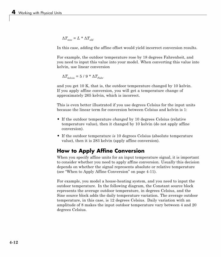
4 Working with Physical Units
ΔTnew = L * ΔTold
In this case, adding the affine offset would yield incorrect conversion results.
For example, the outdoor temperature rose by 18 degrees Fahrenheit, andyou need to input this value into your model. When converting this value intokelvin, use linear conversion
ΔTkelvin = 5 / 9 * ΔTFahr
and you get 10 K, that is, the outdoor temperature changed by 10 kelvin.If you apply affine conversion, you will get a temperature change ofapproximately 265 kelvin, which is incorrect.
This is even better illustrated if you use degrees Celsius for the input unitsbecause the linear term for conversion between Celsius and kelvin is 1:
• If the outdoor temperature changed by 10 degrees Celsius (relativetemperature value), then it changed by 10 kelvin (do not apply affineconversion).
• If the outdoor temperature is 10 degrees Celsius (absolute temperaturevalue), then it is 283 kelvin (apply affine conversion).
How to Apply Affine ConversionWhen you specify affine units for an input temperature signal, it is importantto consider whether you need to apply affine conversion. Usually this decisiondepends on whether the signal represents absolute or relative temperature(see “When to Apply Affine Conversion” on page 4-11).
For example, you model a house-heating system, and you need to input theoutdoor temperature. In the following diagram, the Constant source blockrepresents the average outdoor temperature, in degrees Celsius, and theSine source block adds the daily temperature variation. The average outdoortemperature, in this case, is 12 degrees Celsius. Daily variation with anamplitude of 8 makes the input outdoor temperature vary between 4 and 20degrees Celsius.
4-12
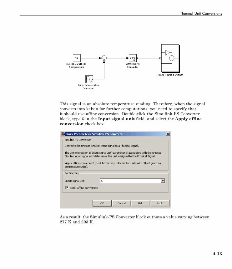
Thermal Unit Conversions
This signal is an absolute temperature reading. Therefore, when the signalconverts into kelvin for further computations, you need to specify thatit should use affine conversion. Double-click the Simulink-PS Converterblock, type C in the Input signal unit field, and select the Apply affineconversion check box.
As a result, the Simulink-PS Converter block outputs a value varying between277 K and 293 K.
4-13
4 Working with Physical Units
Angular UnitsSimscape implementation of angular units relies on the concept of angularunits, specifically radians, being a unit but dimensionless. The notion ofangular units being dimensionless is widely held in the metrology community.The fundamental angular unit, radian, is defined in the Simscape unitregistry as:
pm_addunit('rad', 1, 'm/m');
which corresponds to the SI and NIST definition [1]. In other words, Simscapeunit manager does not introduce a separate dimension, 'angle', with afundamental unit of 'rad' (similar to dimensions for length or mass), butrather defines the fundamental angular unit in terms of meter over meter or,in effect, 1.
The additional angular units, degree and revolution, are defined respectivelyas:
pm_addunit('deg', pi/180, 'rad');pm_addunit('rev', 2*pi, 'rad');
As a result, forward trigonometric functions, such as sin, cos, and tan, workdirectly with arguments expressed in angular units. For example, cosinus of90 degrees equals the cosinus of (pi/2) radians and equals the cosinus of (pi/2).Expansion of forward trigonometric functions works in a similar manner.
Another effect of dimensionless implementation of angular units is theconvenience of the work-energy conversion. For example, torque (in N*m)multiplied by angle (in rad) can be added directly to energy (in J, or N*m). Ifyou specify other commensurate units for the components of this equation,Simscape unit manager performs the necessary unit conversion operationsand the result is the same.
References[1] The NIST Reference on Constants, Units, and Uncertainty,http://physics.nist.gov/cuu/Units/units.html
4-14
5
Using the Simscape EditingMode
• “About the Simscape Editing Mode” on page 5-2
• “Working with Restricted and Full Modes” on page 5-9
• “Editing Mode Information” on page 5-23

5 Using the Simscape™ Editing Mode
About the Simscape Editing Mode
In this section...
“Suggested Workflows” on page 5-2
“What You Can Do in Restricted Mode” on page 5-3
“What You Can Do in Full Mode” on page 5-4
“Switching Between Modes” on page 5-4
“Working with Block Libraries” on page 5-7
Suggested WorkflowsThe Simscape Editing Mode functionality is implemented for customers whoperform physical modeling and simulation using Simscape platform andits add-on products: SimDriveline, SimElectronics®, SimHydraulics, andSimMechanics. It allows you to open, simulate, and save models that containblocks from add-on products in Restricted mode, without checking out add-onproduct licenses, as long as the products are installed on your machine. Itis intended to provide an economical way to distribute simulation modelsthroughout a team or organization.
Note Unless your organization uses concurrent licenses, see the Simscapeproduct page on the MathWorks Web site for specific information on how toinstall add-on products on your machine, to be able to work in Restricted mode.
The Editing Mode functionality supports widespread use of Physical Modelingproducts throughout an engineering organization by making it economical forone user to develop a model and provide it to many other users.
Specifically, this feature allows a user, model developer, to build a model thatuses Simscape platform and one or more add-on products and share thatmodel with other users, model users. When building the model in Full mode,the model developer must have a Simscape license and the add-on productlicenses for all the blocks in the model. For example, if a model combinesSimscape, SimHydraulics, and SimDriveline blocks, the model developerneeds to check out licenses for all three products to work with it in Full mode.
5-2
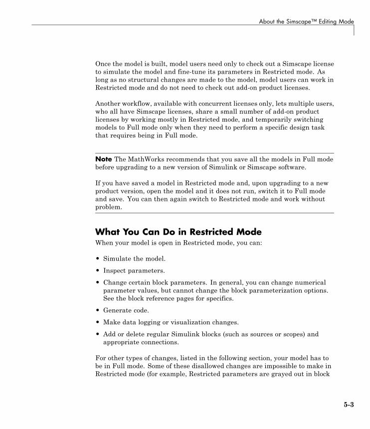
About the Simscape™ Editing Mode
Once the model is built, model users need only to check out a Simscape licenseto simulate the model and fine-tune its parameters in Restricted mode. Aslong as no structural changes are made to the model, model users can work inRestricted mode and do not need to check out add-on product licenses.
Another workflow, available with concurrent licenses only, lets multiple users,who all have Simscape licenses, share a small number of add-on productlicenses by working mostly in Restricted mode, and temporarily switchingmodels to Full mode only when they need to perform a specific design taskthat requires being in Full mode.
Note The MathWorks recommends that you save all the models in Full modebefore upgrading to a new version of Simulink or Simscape software.
If you have saved a model in Restricted mode and, upon upgrading to a newproduct version, open the model and it does not run, switch it to Full modeand save. You can then again switch to Restricted mode and work withoutproblem.
What You Can Do in Restricted ModeWhen your model is open in Restricted mode, you can:
• Simulate the model.
• Inspect parameters.
• Change certain block parameters. In general, you can change numericalparameter values, but cannot change the block parameterization options.See the block reference pages for specifics.
• Generate code.
• Make data logging or visualization changes.
• Add or delete regular Simulink blocks (such as sources or scopes) andappropriate connections.
For other types of changes, listed in the following section, your model has tobe in Full mode. Some of these disallowed changes are impossible to make inRestricted mode (for example, Restricted parameters are grayed out in block
5-3

5 Using the Simscape™ Editing Mode
dialog boxes). Other changes, like changing the physical topology of a model,are not explicitly disallowed, but if you make these changes in Restrictedmode, the software will issue an error message when you try to run, compile,or save such a model.
What You Can Do in Full ModeYou need to open a model in Full mode if you need to do any of the following:
• Add or delete Physical Modeling blocks (that is, Simscape blocks or blocksfrom the add-on product libraries).
• Make or break Physical connections (between Conserving or PhysicalSignal ports).
• Change the types of signals going into actuators or out of sensors (forexample, from velocity to torque).
• Change configuration parameters.
• Change block parameterization options and other restricted parameters.
• Change physical units of parameters.
Switching Between ModesThe following flow chart shows what happens when you switch betweenmodes.
5-4

About the Simscape™ Editing Mode
New models are always created in Full mode. You can then either save themodel in Full mode, or switch to Restricted mode and save the model inRestricted mode.
5-5
5 Using the Simscape™ Editing Mode
When you load an existing model, the license manager checks whether it hasbeen saved in Full or Restricted mode.
• If the model has been saved in Restricted mode, it opens in Restricted mode.
• If the model has been saved in Full mode, the license manager checkswhether all the add-on product licenses for this model are available and, ifso, opens it in Full mode. If a add-on product license is not available, thelicense manager issues an error message and opens the model in Restrictedmode. See also “Example with Multiple Add-On Products” on page 5-6.
Note You can set a Simulink preference to specify that the models are alwaysto open in Restricted mode, regardless of the way they have been saved.
When a model is open, you can transition it between Full and Restrictedmodes at any time, in either direction:
• When you try to switch from Restricted to Full mode, the license managerchecks whether all the add-on product licenses for this model are available.If a add-on product license is not available, the license manager issues anerror message and the model stays in Restricted mode. See also “Examplewith Multiple Add-On Products” on page 5-6.
• No checks are performed when switching from Full to Restricted mode.
Note If a add-on product license has been checked out to open a model in Fullmode, it remains checked out for the remainder of the MATLAB session.Switching to Restricted mode does not immediately return the license.
Example with Multiple Add-On ProductsWhen you try to open a model in Full mode or to switch from Restricted toFull mode, the license manager scans the model and attempts to check outthe required add-on product licenses as it encounters them in the model. If alicense is not available, the license manager issues an error message and themodel stays in Restricted mode. The licenses are checked out sequentially. Asa result, if a model uses blocks from multiple add-on products, some of the
5-6

About the Simscape™ Editing Mode
add-on product licenses may have already been checked out by the time thelicense manager encounters an unavailable license. In this case, these add-onproduct licenses stay checked out until you quit the MATLAB session, eventhough the model is in Restricted mode.
For example, consider a model that uses blocks from SimHydraulics andSimDriveline libraries, but the user who tries to open it has only theSimDriveline license available. It may happen that the license managerchecks out a SimDriveline license first, and then tries to check out aSimHydraulics license, which is not available. The license manager thenissues an error message and opens the model in Restricted mode, but theSimDriveline license stays checked out until the end of the MATLAB session.
Working with Block LibrariesThis section describes the specifics of working with block libraries whileusing the Editing Mode functionality. These rules are applicable to anyphysical modeling blocks, that is, blocks from all Simscape libraries, includingthe add-on products. In general, you need to work in Full mode when youmodify a library block. However, when you open a model that references themodified block, you may work in Restricted mode, under certain conditions.The following summary details the Editing Mode rules for modifying andusing library blocks:
• To add physical modeling blocks to a library block, you need to work inFull mode.
- If this library block had not previously contained physical modelingblocks, you need to work in Full mode to load a preexisting model thatuses this library block or to drag this block to a model.
- If this library block had previously contained physical modeling blocks,you can work in Restricted mode when loading a preexisting model thatuses this library block. However, you have to work in Full mode to dragthis block from the library to a model.
• To add external physical ports to a library block, you need to work in Fullmode.
- You can work in Restricted mode when loading a preexisting model thatuses this library block.
5-7

5 Using the Simscape™ Editing Mode
- However, to connect these additional ports, you need to work in Fullmode because you are changing the model topology.
• To delete external physical ports from a library block, you need to work inFull mode. If these ports were connected in a model saved in Restrictedmode, loading the model causes the topology to change, so you need toswitch to Full mode to save or compile the model.
Resolving Block Library LinksAll Simscape blocks in your models, including the add-on products’ blocks,must have resolved block library links. You can neither disable nor breakthese library links. This is a global requirement of Simscape platform, whichis necessary to enforce the Editing Mode rules for modifying and using libraryblocks, listed above. A model with broken library links will neither compilenor save. You must restore all the broken block library links for your model tobe valid.
If you want to customize certain blocks and use them in your models, youmust add these modified blocks to your own custom library, then copy theblock instances that you need to your model.
5-8

Working with Restricted and Full Modes
Working with Restricted and Full Modes
In this section...
“Setting the Model Loading Preference” on page 5-9
“Saving a Model in Restricted Mode” on page 5-10
“Working with a Model in Restricted Mode” on page 5-13
“Switching from Restricted to Full Mode” on page 5-21
Setting the Model Loading PreferenceBy default, when you load an existing model, the license manager checkswhether it has been saved in Full or Restricted mode and tries to open it inthis mode. However, you can set your preferences so that the models arealways open in Restricted mode, regardless of the way they have been saved.
1 From the MATLAB top menu bar, select File > Preferences. ThePreferences dialog box opens.
2 In the left pane of the Preferences dialog box, select Simscape. The rightpane displays the Editing Mode group box. By default, the Load modelsusing option is set to Editing mode specified in models.
3 Select Restricted mode always from the drop-down list, as shown, andclick OK.
5-9

5 Using the Simscape™ Editing Mode
Now, when you open a model, the license manager does not attempt to checkout add-on product licenses and always opens the model in Restricted mode.
Saving a Model in Restricted ModeRather that setting your preferences so that all the models always open inRestricted mode, you can switch an individual model to Restricted modebefore saving it. Such a model will then, by default, open in Restricted mode.
1 From the top menu bar in the model window, select Simulation >Configuration Parameters. The Configuration Parameters dialog boxopens.
2 In the left pane of the Configuration Parameters dialog box, selectSimscape. The right pane displays the Editing Mode option, which is bydefault set to Full.
3 Select Restricted from the drop-down list, as shown, and click OK.
5-10

Working with Restricted and Full Modes
4 Save the model.
Note The Simscape entry does not appear in the left pane of theConfiguration Parameters dialog box until you add at least one PhysicalModeling block to your model. If you create an additional configuration set fora model, the Simscape entry does not appear in it until you either activateit or perform a Physical Modeling operation, such as adding or deleting aPhysical Modeling block or connection, opening a Physical Modeling blockdialog box, and so on.
Once you have switched a model to Restricted mode, working with it followsthe rules described in “Working with a Model in Restricted Mode” on page
5-11

5 Using the Simscape™ Editing Mode
5-13. Note, however, that the add-on product licenses for this model staychecked out until you quit the MATLAB session.
When you open a model that has been saved in Restricted mode, the licensemanager opens it in Restricted mode and does not check out the add-onproduct licenses.
Example of Saving a Model in Restricted ModeIn this example, you switch a model to Restricted mode and save it.
1 Open the Simple Mechanical System demo model(ssc_simple_mechanical_system).
2 From the top menu bar in the model window, select Simulation >Configuration Parameters. The Configuration Parameters dialog boxopens.
3 In the left pane of the Configuration Parameters dialog box, selectSimscape. The right pane displays the Editing Mode option, which isset to Full by default.
5-12
Working with Restricted and Full Modes
4 Select Restricted from the drop-down list and click OK.
5 Save the model as test_edit_mode.mdl.
Working with a Model in Restricted ModeWhen you open a model in Restricted mode, you can perform a variety oftasks: simulate the model, inspect and fine-tune block parameters, addand delete basic Simulink blocks, and so on. For a complete list of allowedoperations, see “What You Can Do in Restricted Mode” on page 5-3.
When you open a block dialog box in Restricted mode, some of the blockparameters may be grayed out. These are the so-called restricted parametersthat can be modified only in Full mode. In general, you can change numericalparameter values in Restricted mode, but you cannot change the blockparameterization options. See the block reference pages for specifics. Notealso that when a restricted parameter defines the block parameterizationschema, nonrestricted parameters available for fine-tuning in Restricted modedepend on the value of this restricted parameter. For example, in a ConstantVolume Chamber block, the Chamber specification parameter is restricted.If, at the time the model entered Restricted mode, this parameter was setto By volume, then the nonrestricted parameters available for fine-tuningwould be Chamber volume, Specific heat ratio, and Initial pressure. If,however, it was set to By length and diameter, you will have a different setof parameters available in Restricted mode.
You cannot change physical units in Restricted mode. When you open a blockdialog box in Restricted mode, the drop-down lists of units next to a parametername and value are grayed out. When you open a PS-Simulink Converter orSimulink-PS Converter block dialog box, the Unit parameter is grayed out.
The following examples illustrate operations allowed and disallowed inRestricted mode:
• “Simulating and Fine-Tuning a Model in Restricted Mode” on page 5-14
• “Adding and Deleting Simulink Blocks in Restricted Mode” on page 5-17
• “Performing an Operation Disallowed in Restricted Mode” on page 5-19
5-13

5 Using the Simscape™ Editing Mode
Simulating and Fine-Tuning a Model in Restricted ModeThis example shows how you can work with a model in Restricted mode bychanging certain parameter values and observing the simulation results.
1 Open the test_edit_mode model, which you saved in Restricted mode in“Example of Saving a Model in Restricted Mode” on page 5-12. The modelopens in Restricted mode.
2 Open the Joint C Position scope and simulate the model. The models runsand simulates in Restricted mode.
5-14

Working with Restricted and Full Modes
3 Double-click the Wheel and Axle block to open its dialog box. Notice thattheMechanism orientation parameter is grayed out, because you cannotmodify the block driving direction in Restricted mode.
4 Change the Wheel radius parameter value to 0.1.
5-15

5 Using the Simscape™ Editing Mode
5 Simulate the model again. Notice that the motion amplitude of node Cbecame smaller as a result of the wheel radius change.
6 Double-click the Mass block and change theMass parameter value to 24.
7 Simulate the model. Notice that doubling the mass resulted in increasedvibrations.
5-16

Working with Restricted and Full Modes
Adding and Deleting Simulink Blocks in Restricted ModeThis example shows how you can change the model input signal in Restrictedmode by adding and deleting basic Simulink blocks.
1 Open the test_edit_mode model, which you saved in Restricted mode in“Example of Saving a Model in Restricted Mode” on page 5-12. The modelopens in Restricted mode.
2 Open the Joint C Position scope and simulate the model.
5-17

5 Using the Simscape™ Editing Mode
3 Delete the Signal Builder block named Force Input. Replace it with a SineWave block from the Simulink Sources library, as shown below.
4 Simulate the model again. The model successfully compiles and simulatesin Restricted mode.
5-18
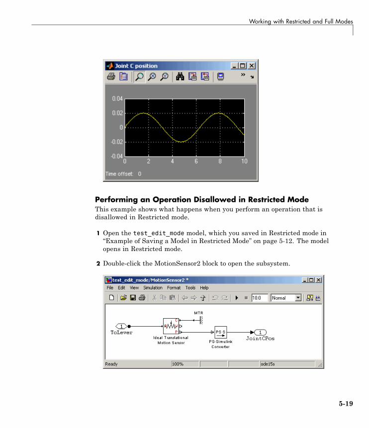
Working with Restricted and Full Modes
Performing an Operation Disallowed in Restricted ModeThis example shows what happens when you perform an operation that isdisallowed in Restricted mode.
1 Open the test_edit_mode model, which you saved in Restricted mode in“Example of Saving a Model in Restricted Mode” on page 5-12. The modelopens in Restricted mode.
2 Double-click the MotionSensor2 block to open the subsystem.
5-19

5 Using the Simscape™ Editing Mode
3 Delete the connection line between port P of the Ideal Translational MotionSensor block and the PS-Simulink Converter block. Instead, connect portV of the Ideal Translational Motion Sensor block to the input port of thePS-Simulink Converter block, to measure the velocity on node C of thelever.
4 Try to simulate the model. An error message appears saying that themodel cannot be compiled because its topology has been changed while inRestricted mode. You can either undo the changes, or switch to Full mode,as described in “Switching from Restricted to Full Mode” on page 5-21.
5-20
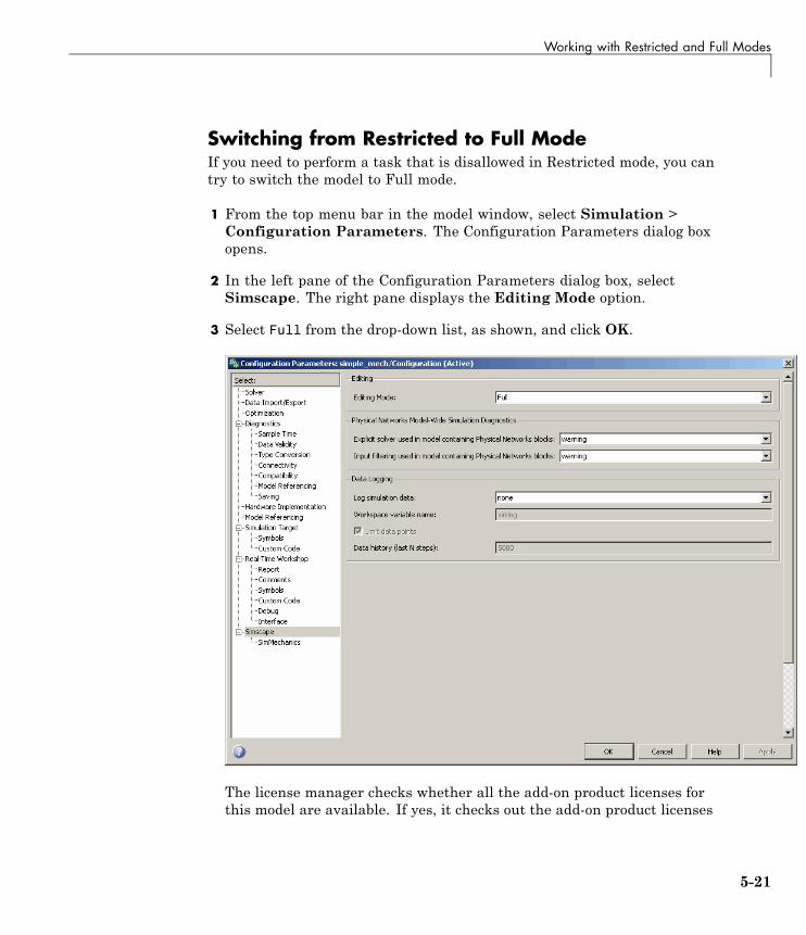
Working with Restricted and Full Modes
Switching from Restricted to Full ModeIf you need to perform a task that is disallowed in Restricted mode, you cantry to switch the model to Full mode.
1 From the top menu bar in the model window, select Simulation >Configuration Parameters. The Configuration Parameters dialog boxopens.
2 In the left pane of the Configuration Parameters dialog box, selectSimscape. The right pane displays the Editing Mode option.
3 Select Full from the drop-down list, as shown, and click OK.
The license manager checks whether all the add-on product licenses forthis model are available. If yes, it checks out the add-on product licenses
5-21

5 Using the Simscape™ Editing Mode
and switches the model to Full mode. If a add-on product license is notavailable, the license manager issues an error message and the model staysin Restricted mode.
Note If the switch to Full mode fails but some of the add-on product licenseshave already been checked out, they stay checked out until you quit theMATLAB session. For more information, see “Example with Multiple Add-OnProducts” on page 5-6.
Once the model is switched to Full mode, you can perform the needed designand simulation tasks, and then either save it in Full mode, or switch back toRestricted mode and save it in Restricted mode.
5-22

Editing Mode Information
Editing Mode Information
In this section...
“What Is the Current Mode?” on page 5-23
“Which Licenses Are Checked Out?” on page 5-23
What Is the Current Mode?If you are unsure whether the model is currently open in Restricted or Fullmode, you can check by following these steps.
1 From the top menu bar in the model window, select Simulation >Configuration Parameters. The Configuration Parameters dialog boxopens.
2 In the left pane of the Configuration Parameters dialog box, selectSimscape. The right pane displays the Editing Mode option, which iseither Full or Restricted.
3 At this point, you can either try switching the mode by selecting a differentoption from the drop-down list, or click Cancel to stay in the current mode.
Which Licenses Are Checked Out?Use the MATLAB license command to get a list of all the licenses currentlyin use. In the MATLAB Command Window, type
license('inuse')
This command returns a list of licenses checked out in the current MATLABsession. In the list, products are listed alphabetically by their license featurenames.
5-23

5 Using the Simscape™ Editing Mode
5-24

A
Examples
Use this list to find examples in the documentation.

A Examples
Getting Started“Creating a Simple Model” on page 1-17
Best Practices“Grounding Rules” on page 1-35“Example of Using a Parasitic Resistance to Avoid Numerical SimulationIssues” on page 1-39
Editing Mode“Example of Saving a Model in Restricted Mode” on page 5-12“Simulating and Fine-Tuning a Model in Restricted Mode” on page 5-14“Adding and Deleting Simulink Blocks in Restricted Mode” on page 5-17“Performing an Operation Disallowed in Restricted Mode” on page 5-19
A-2
Index
IndexEelectrical ground
specifying 1-35
Llinearizing
Simscape™ models 2-28
Nnumerical simulation issues
avoiding 1-38
Ooperating points
finding in Simscape™ models 2-22linearizing Simscape™ models at 2-28
Pports
physical conserving 1-9physical signal 1-9
SSimscape Editing Mode 5-2
Full mode 5-4
information 5-23Restricted mode 5-3saving in Restricted mode 5-10switching between modes 5-4workflows 5-2working in Restricted mode 5-13working with block libraries 5-7
Simscape softwareblock library structure 1-11editing modes 5-2logging simulation data 3-2
Ttrimming
Simscape™ models 2-22
Uunits
defining physical units 4-4
Vvariables
across 1-4direction 1-6through 1-4using in model equations 1-5
Index-1