MatlabforCS6320Beginners

Basics: Starting Matlab 

o CADE Lab remote access 

 o Student version on your own computer 

  Change the Current Folder to the directory where your programs, images, etc. will be stored 

     

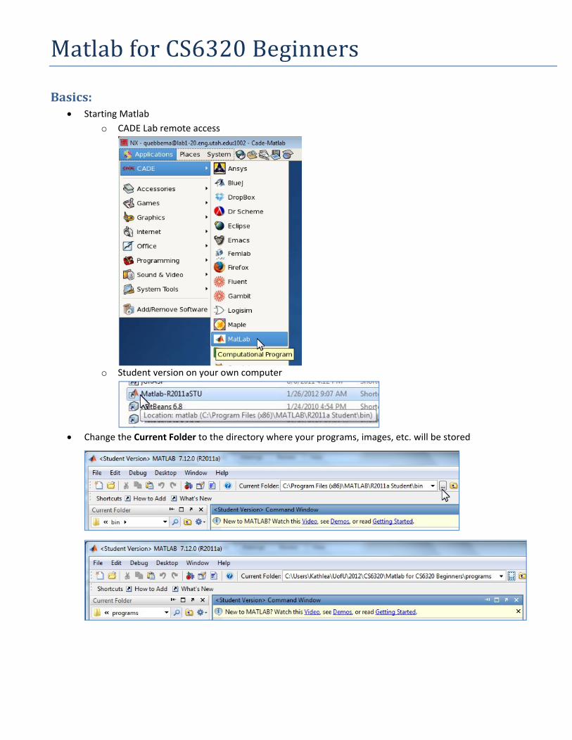
Getting help from Matlab(primers, tutorials, online help) 

 

 

o If you are a Matlab beginner you can click on Getting Started for general help with how Matlab works or 

click on User's Guide | Programming fundamentals | Syntax Basics for basic information such as how 

variables are created and initialized in Matlab. 

o An excellent description of Matlab expressions can be found in Getting Started | Matrices and Arrays | 

Expressions. It points out the fact that Matlab stands for "Matrix Laboratory". Whenever possible use a 

matrix expression instead of a for loop to make matrix calculations. These expressions will execute 

much faster than nested for loops, because Matlab is optimized for manipulating matrices. 

   

Creating, writing and running programs (m‐files) 

o You can run commands in the Command Window to try out how they work 

o For automatically running commands, create an m‐file. This is the "source code" for MatLab programs. 

m‐files are interpreted programs, called scripts, and are not compiled before running. Remember: 

Matlab is a "Computational Program", not your usual programming language. 

o m‐files can be created in two ways: type edit in the Command window or click on the Actions icon in 

the Current Folder window and select New File | Script: 

  

 

 

 

 

 

 

o The Editor ‐ Untitled window will pop up (when you save it you can give it a name): 

 

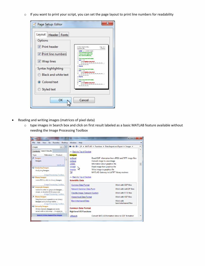
o If you want to print your script, you can set the page layout to print line numbers for readability 

 

 

Reading and writing images (matrices of pixel data) 

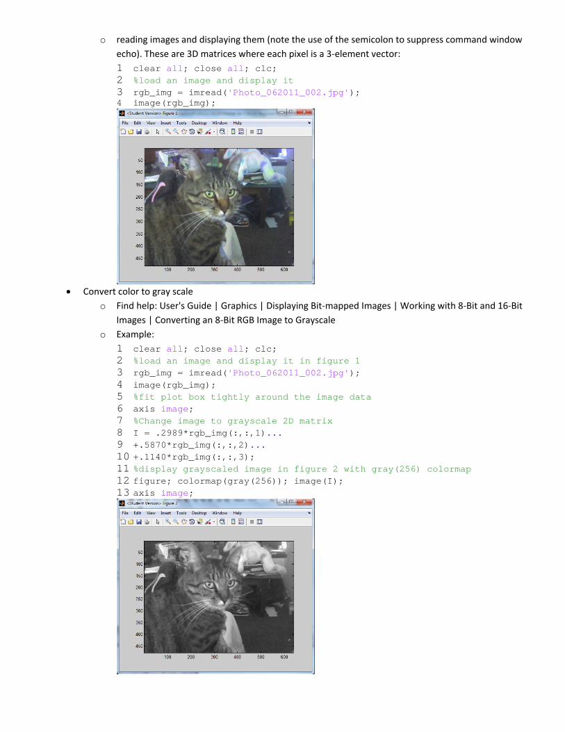
o type images in Search box and click on first result labeled as a basic MATLAB feature available without 

needing the Image Processing Toolbox 

 

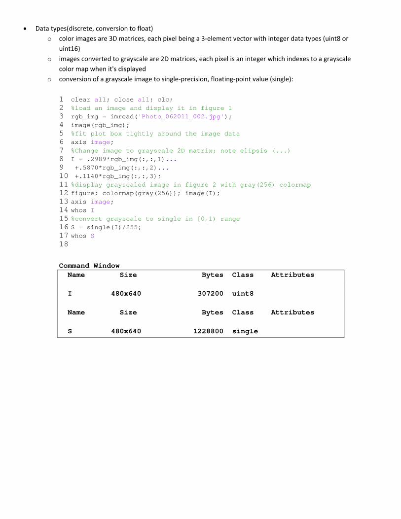
o reading images and displaying them (note the use of the semicolon to suppress command window 

echo). These are 3D matrices where each pixel is a 3‐element vector: 

1 clear all; close all; clc; 2 %load an image and display it 3 rgb_img = imread('Photo_062011_002.jpg'); 4 image(rgb_img);

Convert color to gray scale 

o Find help: User's Guide | Graphics | Displaying Bit‐mapped Images | Working with 8‐Bit and 16‐Bit 

Images | Converting an 8‐Bit RGB Image to Grayscale 

o Example: 

1 clear all; close all; clc; 2 %load an image and display it in figure 1 3 rgb_img = imread('Photo_062011_002.jpg'); 4 image(rgb_img); 5 %fit plot box tightly around the image data 6 axis image; 7 %Change image to grayscale 2D matrix 8 I = .2989*rgb_img(:,:,1)... 9 +.5870*rgb_img(:,:,2)... 10 +.1140*rgb_img(:,:,3); 11 %display grayscaled image in figure 2 with gray(256) colormap 12 figure; colormap(gray(256)); image(I); 13 axis image;

Display images(multiple) 

o figure, image, and subplot 

1 clear all; close all; clc; 2 %load an image and display it in first row, 1st column, figure 1 3 im1 = imread('Photo_062011_002.jpg'); 4 subplot(2,2,1);image(im1); 5 %fit plot box tightly around the image data 6 axis image; 7 %Change image to grayscale 2D image 8 I = .2989*im1(:,:,1)... 9 +.5870*im1(:,:,2)... 10 +.1140*im1(:,:,3); 11 %display grayscaled image in 1st row, 2nd column, figure 1 12 subplot(2,2,2); colormap(gray(256)); image(I); 13 axis image; 14 %load another image and display it in second row, 1st column figure 1 15 im2 = imread('IMG_1766.jpg'); 16 subplot(2,2,3); image(im2); 17 axis image; 18 %load 3rd color image and display it in second row, 2nd column figure 1 19 im3 = imread('IMG_1768.jpg'); 20 subplot(2,2,4); image(im3); 21 axis image;  

 

writing images: 

1 clear all; close all; clc; 2 %load an image and display it in figure 1 3 rgb_img = imread('Photo_062011_002.jpg'); 4 image(rgb_img); 5 %fit plot box tightly around the image data 6 axis image; 7 %Change image to grayscale 2D matrix; note elipsis (...) 8 I = .2989*rgb_img(:,:,1)... 9 +.5870*rgb_img(:,:,2)... 10 +.1140*rgb_img(:,:,3); 11 %display grayscaled image in figure 2 with gray(256) colormap 12 figure; colormap(gray(256)); image(I); 13 axis image; 14 %write grayscaled image to new file 15 imwrite(I,gray(256),'grayStarbuck.jpg','jpg');

File: grayStarbuck.jpg

 

 

Data types(discrete, conversion to float) 

o color images are 3D matrices, each pixel being a 3‐element vector with integer data types (uint8 or 

uint16) 

o images converted to grayscale are 2D matrices, each pixel is an integer which indexes to a grayscale 

color map when it's displayed 

o conversion of a grayscale image to single‐precision, floating‐point value (single): 

 

1 clear all; close all; clc; 2 %load an image and display it in figure 1 3 rgb_img = imread('Photo_062011_002.jpg'); 4 image(rgb_img); 5 %fit plot box tightly around the image data 6 axis image; 7 %Change image to grayscale 2D matrix; note elipsis (...) 8 I = .2989*rgb_img(:,:,1)... 9 +.5870*rgb_img(:,:,2)... 10 +.1140*rgb_img(:,:,3); 11 %display grayscaled image in figure 2 with gray(256) colormap 12 figure; colormap(gray(256)); image(I); 13 axis image; 14 whos I 15 %convert grayscale to single in [0,1) range 16 S = single(I)/255; 17 whos S 18

Command Window Name Size Bytes Class Attributes I 480x640 307200 uint8 Name Size Bytes Class Attributes S 480x640 1228800 single

Read cursor position and values (manual definition of features) 

1 clear all; close all; clc; 2 rgb_img = imread('Photo_062011_002.jpg'); 3 I = .2989*rgb_img(:,:,1)... 4 +.5870*rgb_img(:,:,2)... 5 +.1140*rgb_img(:,:,3); 6 %display grayscaled image in figure 2 with gray(256) colormap 7 fig = figure; colormap(gray(256)); image(I); 8 axis image; 9 %get data object 10 dcm_obj = datacursormode(fig); 11 %enable cursormode 12 set(dcm_obj,'DisplayStyle','datatip',... 13 'SnapToDataVertex','on','Enable','on') 14 %prompt user 15 disp('Click on the image to display a data tip, then press Return.') 16 pause % Wait while the user does this. 17 %save cursor position and display in Command Window 18 c_info = getCursorInfo(dcm_obj); 19 pos = c_info.Position 20

 

Command Window Click on the image to display a data tip, then press Return. pos = 379 193

Overlay gray scale image with processed binary (logical data type) image information(color overlay) 

pointoperation: Thresholding an image (binarize) with specified threshold. 

Filtering: Neighborhood filter: 

o Averaging (smoothing) 

o Edge detection(x,y derivatives, magnitude ‐> edge image) 

o Application: overlay binarized edge image with original