MATLAB‑based algorithm to estimate depths of isolated thin dike‑like sources using higher‑order horizontal derivatives of magnetic anomaliesYunus Levent Ekinci1,2*

BackgroundGeomagnetic surveys aim to investigate subsurface geology through the anomalies in the Earth’s magnetic field originating from magnetic minerals contained in subsurface rocks (Kearey et  al. 2002). The estimation of model parameters of magnetic sources, such as location, depth, thickness, dip, size, shape, extension, and magnetic susceptibil-ity, is extremely important in the interpretation stage. However, the well-known complex nature of the magnetic anomalies may complicate the interpretation. According to the Gauss theorem, if the potential field is known only on a bounding surface, there may be infinitely many equivalent causative source distributions inside the boundary that can

Abstract

This paper presents an easy-to-use open source computer algorithm (code) for esti-mating the depths of isolated single thin dike-like source bodies by using numerical second-, third-, and fourth-order horizontal derivatives computed from observed mag-netic anomalies. The approach does not require a priori information and uses some fil-ters of successive graticule spacings. The computed higher-order horizontal derivative datasets are used to solve nonlinear equations for depth determination. The solutions are independent from the magnetization and ambient field directions. The practical usability of the developed code, designed in MATLAB R2012b (MathWorks Inc.), was successfully examined using some synthetic simulations with and without noise. The algorithm was then used to estimate the depths of some ore bodies buried in different regions (USA, Sweden, and Canada). Real data tests clearly indicated that the obtained depths are in good agreement with those of previous studies and drilling information. Additionally, a state-of-the-art inversion scheme based on particle swarm optimiza-tion produced comparable results to those of the higher-order horizontal derivative analyses in both synthetic and real anomaly cases. Accordingly, the proposed code is verified to be useful in interpreting isolated single thin dike-like magnetized bodies and may be an alternative processing technique. The open source code can be easily modified and adapted to suit the benefits of other researchers.

Keywords: Depth determination, Magnetic anomalies, Higher-order horizontal derivatives, Dike-like magnetized bodies, Open source code

Open Access

© 2016 The Author(s). This article is distributed under the terms of the Creative Commons Attribution 4.0 International License (http://creativecommons.org/licenses/by/4.0/), which permits unrestricted use, distribution, and reproduction in any medium, provided you give appropriate credit to the original author(s) and the source, provide a link to the Creative Commons license, and indicate if changes were made.

RESEARCH

Ekinci SpringerPlus (2016) 5:1384 DOI 10.1186/s40064‑016‑3030‑7

*Correspondence: ylekinci@beu.edu.tr 1 Department of Archaeology, Faculty of Arts and Sciences, Bitlis Eren University, 13000 Bitlis, TurkeyFull list of author information is available at the end of the article

Page 2 of 15Ekinci SpringerPlus (2016) 5:1384

produce the same anomaly characterization (Li and Oldenburg 1996). In some cases, remanent magnetization mostly produces noteworthy effects, which may lead to incor-rect interpretations if overlooked (Telford et al. 1990). Data processing techniques notice-ably assist in the interpretation of potential field anomalies and may also aid in geological implications and mapping (Blakely 1995). Hence, depending on the objectives of analyses and studies, many processing techniques have been reported for interpreting potential field anomalies. If potential field  data quality permits, numerous analysing procedures can be conducted that facilitate in building a general understanding of the details of caus-ative bodies (Ekinci and Yiğitbaş 2012, 2015; Balkaya et al. 2012; Ekinci et al. 2013, 2014).

Generally, model parameters of causative structures are frequently analysed and esti-mated using spectral methods, inversion and modelling techniques, graphical methods, and other numerical methods (Ekinci and Sarı 2008). To determine model parameters such as source depth, magnetic anomalies are commonly interpreted using some sim-ple-shaped geometric source bodies such as point source, sheet, sphere, horizontal and vertical cylinders, and prism (Gay 1963, 1965; Mohan et  al. 1982; Prakasa Rao et  al. 1986; Rao and Babu 1991; Abdelrahman and Sharafeldin 1996). Further, some studies have reported a number of automatic methods, such as Werner (Werner 1953) and Euler (Thompson 1982; Reid et al. 1990) deconvolution methods, in which the depth estima-tion problem is transformed into the problem of determining a solution to a system of linear equations (Abdelrahman and Abo-Ezz 2001). One of the efficient  numerical methods to estimate the depth at the top of a isolated dike-like body involves analys-ing the numerical second-, third-, and fourth-order horizontal derivative anomalies of magnetic data computed using some filters of successive graticule spacings (Abdelrah-man and Abo-Ezz 2001). By considering many recent studies focused on determining the depths to the top of isolated thin dike-like magnetic sources (Bastani and Pedersen 2001; Abdelrahman and Essa 2005; Asfahani and Tlas 2007; Tlas and Asfahani 2011a, b; Cooper 2012, 2014, 2015), it was assumed that it might be favourable to develop a com-puter code to implement a depth-determination procedure for the benefit of scientific studies and investigations. The algorithm based on the use of higher-order horizontal derivative analyses is designed using MATLAB R2012b (Mathworks Inc.). To evaluate the efficiency of the developed code, synthetically produced magnetic anomalies with and without noise and some real magnetic anomalies from Arizona (USA), Kiirnu-navaara (Sweden), and Ontario (Canada) were analysed. Applications clearly  showed that the results obtained from the proposed code, particle swarm optimization (PSO), and previous studies are comparable.

MethodsHigher‑order horizontal derivative analyses and depth determination

The general expression for a magnetic anomaly either in total, vertical, or horizontal fields of an arbitrary magnetized thin dike-like structure is given by (Gay 1963; Atchuta Rao et al. 1980; Sundararajan et al. 1985; Abdelrahman and Sharafeldin 1996; Asfahani and Tlas 2007; Tlas and Asfahani 2011a, b)

(1)T(xi, xo, A, z, θ) = A

z cos θ+ (xi − xo) sin θ

(xi − xo)2 + z2

i = 1, 2, 3, 4, 5, . . . , N

Page 3 of 15Ekinci SpringerPlus (2016) 5:1384

where A = K z, and z represents the depth to the top of the magnetized thin dike, K is the amplitude coefficient or effective intensity of magnetization, θ is the effective angle of magnetization or the index parameter, and x and xo represent the horizontal position coordinates on the profile and the exact origin of the anomaly, respectively. By using this formula, it is implicitly assumed that the source structure is perpendicular to the profile direction. To implement the depth estimation procedure, numerical values of the higher-order horizontal derivatives of magnetic data are required. Second-order hori-zontal derivatives are obtained by

where T2 represents the second-order horizontal derivative, T represents the magnetic data, x is the horizontal position coordinate, and s is the graticule spacing or numeric sample interval (i.e., 2, 3, 4, and 5). The nonlinear equation used for depth estimation is derived using Eq. (1) and is given by the following expression (see Abdelrahman and Abo-Ezz 2001 for detailed descriptions)

where

where T2 (0) represents the origin of the profile, which can be located practically by draw-ing a straight line joining the maximum and minimum values of the magnetic anomaly profile and locating the vertical axis by its intersection with the anomaly curve (Stanley 1977; Abdelrahman and Hassanein 2000; Abdelrahman and Abo-Ezz 2001; El-Araby 2003; Abdelrahman et  al. 2012). In Eq.  (3), the right- and left-hand terms involve the parameter z, which is the depth to the top of the dike-like magnetic source. This nonlin-ear equation is solved easily by using an iterative method (Press et al. 2007) in the form of

where zu is the updated depth and zi is the initial depth (close to zero; e.g., 1e-1). In each iteration, zu is used as the initial estimate and the iteration terminates when the differ-ence between zu and zi reaches a user-defined small value close to zero (e.g., 1e-5). By using the simple finite-difference approximation, the third-order horizontal derivatives of the magnetic data are obtained as follows

and the nonlinear equation derived from Eq. (1) becomes

(2)T2(xi) =T(xi + 2s)− 2T(xi)+ T(xi − 2s)

(2s)2

(3)z =

[

F(

9s2 + z2)(

s2 + z2)[

z3 − z(

4s2 + z2)]

(

4s2 + z2)[(

s2 + z2)

(z)−(

9s2 + z2)

(z)]

]1/2

(4)F =T2(s)+ T2(−s)

T2(0)

(5)zu = f(zi)

(6)T3(xi) =T(xi + 3s)− 3T(xi + s)+ 3T(xi − s)− T(xi − 3s)

(2s)3

(7)z =

[(

3F(

4s2 + z2)(

16s2 + z2)

4(

9s2 + z2)

[

(

s2 + z2)

−(

9s2 + z2)

(

4s2 + z2)

−(

16s2 + z2)

])

− s2

)1/2

Page 4 of 15Ekinci SpringerPlus (2016) 5:1384

where

determines the depth to the top of the magnetized body by using third-order horizontal derivatives (Abdelrahman and Abo-Ezz 2001). Similarly, by using the finite-difference approximation, numerical values of fourth-order horizontal derivatives are obtained by

and the nonlinear depth equation derived from Eq.  (1) is given as (Abdelrahman and Abo-Ezz 2001)

where

Again, Eq. (5) is used to determine the global minimum.

Inversion through PSO

It is known that global optimization algorithms as samplers are more suitable for achiev-ing sampling during optimization. The main advantage of these algorithms is their abil-ity to escape from local minima by performing a stochastic search within the model space (Balkaya 2013; Ekinci et al. 2016). Moreover, to determine the global minimum, they do not need a well-constructed initial estimate as they provide a robust and versa-tile search process. PSO (Kennedy and Eberhart 1995), a global optimization method, is one of the popular naturally inspired metaheuristic algorithms based on the behav-iour of bird flocks and fish schools searching for food (Pallero et  al. 2015). In brief, a user-defined objective function is optimized through a swarm of particles, searching the space of model parameters, whose responses are similar to the observed data. This stochastic population-based search algorithm is initialized by assigning a population of particles (a group of model parameters) with random positions (x) and velocities (v) in the search space (Göktürkler and Balkaya 2012). During inversion, position and velocity of each particle are updated using the following equations (Kennedy and Eberhart 1995; Shi and Eberhart 1998)

(8)F =T3(s)+ T3(−s)

T3(0)

(9)T4(xi) =T(xi + 4s)− 4T(xi + 2s)+ 6T(xi)− 4T(xi − 2s)+ T(xi − 4s)

(2s)4

(10)z =

[

FA

B

]1/2

(11)F =T4(s)+ T4(−s)

T4(0)

(12)A =

(

z2(

4s2 + z2)

(z)− 4z2(

16s2 + z2)

(z)+ 3z(

16s2 + z2)(

4s2 + z2))

(

16s2 + z2)(

4s2 + z2)

(13)B =2z

(

s2 + z2) −

3z(

9s2 + z2) +

z(

25s2 + z2)

Page 5 of 15Ekinci SpringerPlus (2016) 5:1384

where vki is the velocity of the particle i at the kth iteration, xki is the current i model at kth iteration, w represents the value of the inertia weight (0 < w < 1), and c1 and c2 are the coefficients controlling the particle’s individual (i.e., best local value) and social behaviours (i.e., best global value), respectively. The symbols r1 and r2 are the random number generators (Press et al. 1994) drawn uniformly in the open interval [0, 1] (Srivas-tava and Agarval 2010). The iteration terminates after reaching the maximum number of iterations defined by the user or obtaining the desired objective function value (Shi and Eberhart 1998; Poli et al. 2007; Luke 2009; Salmon 2011; Peksen et al. 2011, 2014; Gök-türkler and Balkaya 2012), which is defined as follows

where the superscript T is the matrix transpose, N is the amount of data, and dobs and dcal represent the magnetic anomalies observed and calculated at T(xi). In this study, 10 independent runs were performed using 100 particles to obtain the optimum model parameters. Values 1, 2, and 2 were assigned for the inertia weight (w) and the cogni-tive and social scaling factors (c1 and c2), respectively (Kennedy and Eberhart 1995). The root-mean-square values were calculated by obtaining the square root of Eq. (15).

The computer algorithmThe developed MATLAB-based code (HigherDerivatives.m) analyses magnetic profile datasets using higher-order horizontal derivatives. During code execution, the procedure first loads the two-column profile dataset, which is written in SURFER data (*.dat) file format (GOLDEN SOFTWARE). The first and second columns include the horizontal distances of the observation points over the profile and the corresponding magnetic read-ings, respectively. An input dialog box is then opened to store the sampling interval of the profile in meters and the maximal graticule spacing number. Although, the default value for the maximal graticule spacing number is five, the user can increase the number if the length of the dataset is suitable. Next, the designed algorithm computes the higher-order horizontal derivative data for the given graticule spacing values and displays them on the screen via a MATLAB figure. After computing the depths by utilizing the afore-mentioned nonlinear equations, the derived results are stored in a text file compatible with a Microsoft text document. The developed open source algorithm (Additional file 1: HigherDerivatives) and synthetic datasets (Additional file 2: Figure1data and Additional file 3: Figure2data) are given as Additional files in text format. The code and datasets must be copied into a MATLAB.m file and a worksheet in the SURFER program, respectively.

Test studiesSynthetic data examples

First, the efficiency of the developed algorithm was tested by constructing some syn-thetic simulations with and without noise. Synthetic magnetic dataset was generated using Eq.  (1). Figure 1a demonstrates the magnetic anomaly of the noise-free example

(14)vk+1i = wvki + c1r1

(

pki − xki

)

+ c2r2

(

gki − xki

)

xk+1i = xki + vki

(15)Err = [dobs − dcal]T· [dobs − dcal]/N

Page 6 of 15Ekinci SpringerPlus (2016) 5:1384

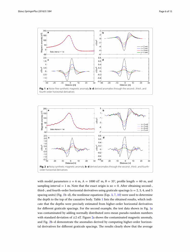
with model parameters z = 6 m, A = 1000 nT m, θ = 35°, profile length = 60 m, and sampling interval = 1 m. Note that the exact origin is xo = 0. After obtaining second-, third-, and fourth-order horizontal derivatives using graticule spacings (s = 2, 3, 4, and 5 spacing units) (Fig. 1b–d), the nonlinear equations (Eqs. 3, 7, 10) were used to determine the depth to the top of the causative body. Table 1 lists the obtained results, which indi-cate that the depths were precisely estimated from higher-order horizontal derivatives for different graticule spacings. For the second example, the test data shown in Fig. 1a was contaminated by adding normally distributed zero-mean pseudo-random numbers with standard deviation of ±2 nT. Figure 2a shows the contaminated magnetic anomaly, and Fig. 2b–d demonstrate the anomalies derived by computing higher-order horizon-tal derivatives for different graticule spacings. The results clearly show that the average

Fig. 1 a Noise-free synthetic magnetic anomaly, b–d derived anomalies through the second-, third-, and fourth-order horizontal derivatives

Fig. 2 a Noisy synthetic magnetic anomaly, b–d derived anomalies through the second-, third-, and fourth-order horizontal derivatives

Page 7 of 15Ekinci SpringerPlus (2016) 5:1384

depths obtained from higher-order horizontal derivatives are very close to each other (Table 1). When considering the standard deviations of obtained depths, the third-order derivative produced an optimum result (5.94 ± 0.39 m). Although there is artificial noise in the magnetic dataset, the obtained average depth seemed to be very convincing. Addi-tionally, the results obtained through higher-order horizontal derivative analyses were compared with those obtained using one of the state-of-the-art inversion techniques, namely PSO. As mentioned earlier, the inversion process was repeated 10 times by using different starting models, and the model having the minimum objective-function value (i.e., error) was considered the best-fitting model. Table  2 lists the search space parameters for PSO and the estimated depths. Figure 3 shows observed and calculated magnetic anomalies for both noise-free and noisy examples. According to the closeness of the results obtained using higher-order horizontal  derivative analyses and the PSO technique in the synthetic examples, it was considered beneficial to compare the results obtained using the developed code with both PSO algorithm and previous studies to evaluate the effectiveness of the proposed code for real data cases.

Table 1 The depths obtained through higher-order horizontal derivative analyses for syn-thetic magnetic anomalies

Graticule spacing (s)

Second order derivative Third order derivative Fourth order derivative

Estimated depth (m)

Iteration number

Estimated depth (m)

Iteration number

Estimated depth (m)

Iteration number

Synthetic model without noise

2 6.00 36 6.00 26 6.00 27

3 6.00 26 6.00 18 6.00 22

4 6.00 21 6.00 15 6.00 19

5 6.00 17 6.00 13 6.00 16

Synthetic model with noise

2 5.14 31 6.05 26 4.82 24

3 6.30 27 5.44 17 6.44 23

4 5.79 20 6.39 16 5.81 18

5 6.15 18 5.87 13 6.17 17

Average depth (m)

5.84 ± 0.52 5.94 ± 0.39 5.81 ± 0.71

Table 2 Search space ranges and estimated parameters for synthetic magnetic anomalies

Model par. True values

Search spaces Estimated parameters

Min. Max. Noise‑free data Noisy data

z (m) 6 1 20 6.04 6.11

θ −35 −90 90 −35.23 −36.23

A (nT m) 1000 10 10e3 1004.84 1015.97

rms (nT) 0.30 2.44

Run number at which the best solution obtained

2 1

Page 8 of 15Ekinci SpringerPlus (2016) 5:1384

Real data examples

After the successful synthetic experiments, magnetic anomalies of a copper mine (Ari-zona, USA), an iron mine (Kiirunavaara, Sweden), and an olivine diabase dike (Ontario, Canada) were considered for investigating the effectiveness of the developed code on field datasets.

Pima copper mine, Arizona, USA

The first example includes a vertical component magnetic anomaly (Fig.  4a) obtained from the Pima copper mine, Arizona, USA (Gay 1963), which has been a major industry since the nineteenth century. The Pima mining district is one of the largest porphyry copper districts in USA. Mineralization related to Laramide igneous activity is known to occur in Paleozoic sedimentary rocks, Mesozoic sedimentary and volcanic sequences, and in Paleocene igneous rocks (Shafiqullah and Langlois 1978). The 728 m long verti-cal magnetic anomaly profile was digitized using a sampling interval of 13 m (Fig. 4a). The digitized magnetic anomaly was used to obtain the depth to the top of the ore body. Figure  4b–d show the anomalies derived from the use of different higher-order hori-zontal  derivatives for different successive graticule spacings (s =  2, 3, 4, and 5). After

Fig. 3 Synthetic magnetic datasets and the anomalies calculated by using the best-fitting model parameters obtained from PSO algorithm. a Noise-free example, b noisy example

Fig. 4 a Vertical component magnetic anomaly over Pima copper mine, Arizona, USA (adapted from Abdel-rahman and Sharafeldin (1996), p 219), b–d derived anomalies through the second-, third-, and fourth-order horizontal derivatives

Page 9 of 15Ekinci SpringerPlus (2016) 5:1384

obtaining the horizontal derivative anomalies, Eqs. 3, 7, and 10 were applied to compute the depth to the top of the copper ore dike. Table 3 shows the results: the average depths obtained from second-, third-, and fourth-order horizontal derivatives do not differ from each other significantly. The one with the lowest standard deviation yielded the opti-mal approximation. The depth to the top of the ore body computed using the developed algorithm is 67.9 m. The depth of this dike structure was previously reported by several researchers through different algorithms, and was recorded as 69.8 m (Gay 1963), 66 m (Abdelrahman and Sharafeldin 1996), 71.5 m (Asfahani and Tlas 2007), 71.25 m (Tlas and Asfahani 2011a), and 60 m (Abdelrahman and Essa 2015). Thus, the depth obtained using the developed code is very close to those of previous studies. Additionally, using the search space values, shown in Table 4, PSO algorithm produced a solution of 68.3 m (Fig. 7a), which matches well with the depth obtained using the developed code. Nota-bly, the actual depth of the top of this thin dike body obtained by drilling is approxi-mately 64 m (Gay 1963).

Kiirunavaara iron mine, Sweden

The second field example is the vertical component of the magnetic anomaly observed at Kiirunavaara iron mine (northern Sweden), which is the largest of the apatite iron ores in Sweden. The Kiirunavaara group or Kiruna porphyries host economically important iron oxide-apatite deposits in the Kiruna and Malmberget areas (Lynch and Jönberger 2014). The vertical component magnetic anomaly used in this study is due to a vein of approxi-mately 20  % magnetite (Grant and West 1965). The 600  m long vertical component

Table 3 The depths obtained through higher-order horizontal derivative analyses for Ari-zona (USA) vertical magnetic anomaly

Graticule spacing (s)

Second order derivative Third order derivative Fourth order derivative

Estimated depth (m)

Iteration number

Estimated depth (m)

Iteration number

Estimated depth (m)

Iteration number

2 64.12 30 58.30 20 60.54 23

3 65.20 22 56.26 14 61.62 19

4 69.39 19 61.43 13 68.89 17

5 72.78 16 68.19 12 74.35 16

Average depth (m)

67.87 ± 3.99 61.05 ± 5.22 66.35 ± 6.5

Table 4 Search space ranges and  estimated parameters for  Arizona (USA)  vertical mag-netic anomaly

Model par. Search spaces Estimated parameters

Min. Max. Arizona data

z (m) 1 200 68.29

θ −90 90 −50.76

A (nT m) 10 10e4 39267.31

rms (nT) 10.88

Run number at which the best solution obtained

2

Page 10 of 15Ekinci SpringerPlus (2016) 5:1384

magnetic anomaly was digitized with a sampling interval of 12 m (Fig. 5a). Figure 5b–d illustrate the anomalies obtained from higher-order horizontal derivatives for different graticule spacings. Table 5 lists the depths at the top of the ore body computed through Eqs. 3, 7, and 10. The results clearly show that the depths obtained by the use of second- and fourth-order horizontal derivatives are very close to each other, whereas the depth computed through the third-order horizontal derivative differs significantly. This may be due to the regional background, as suggested by Abdelrahman and Abo-Ezz (2001). The lowest standard deviation for the depths was obtained from the second-order horizon-tal derivatives and the average depth obtained is 65.4 m, which is close to the results of other studies: 59 m by Sundararajan et al. (1985) and 62–63 m by Grant and West (1965). Table 6 lists the search ranges used and the parameters obtained from PSO inversion. The PSO algorithm yielded a depth of 56.1 m (Table 6; Fig. 7b), which moderately sup-ports the results of the higher-order horizontal derivative analyses.

Diabase dike, Pishabo Lake, Ontario, Canada

The third example is a total field magnetic anomaly observed above an outcropping of a gabbroic olivine diabase dike, which intersects the northwestern arm of Pishabo Lake,

Fig. 5 a  Vertical component magnetic anomaly over Kiirunavaara iron mine, Sweden (adapted from Sunda-rarajan et al. (1985), p 564), b–d derived anomalies through the second-, third-, and fourth-order horizontal derivatives

Table 5 The depths obtained through higher-order horizontal derivative analyses for Kiiru-navaara (Sweden) vertical magnetic anomaly

Graticule spacing (s)

Second order derivative Third order derivative Fourth order derivative

Estimated depth (m)

Iteration number

Estimated depth (m)

Iteration number

Estimated depth (m)

Iteration number

2 69.39 35 28.31 12 71.07 27

3 66.46 24 30.95 11 66.82 21

4 63.07 19 47.55 12 63.86 17

5 62.59 15 49.66 11 63.51 15

Average depth (m)

65.38 ± 3.18 39.12 ± 11.04 66.32 ± 3.5

Page 11 of 15Ekinci SpringerPlus (2016) 5:1384

Ontario, Canada (McGrath and Hood 1970). The airborne total field magnetic data have been collected with a flight elevation of approximately 304 m (McGrath and Hood 1970). The dike having a width of approximately 220 m (Abdelrahman et  al. 2007) has been described as being composed of plagioclase, augite, biotite, apatite, olivine, and large patches of magnetite (El-Araby 2003). The other geological units in the study area are the granite gneiss and greywacke (McGrath and Hood 1970). A sampling interval of 40  m was used to digitize the 2000 m long total field magnetic anomaly. The digitized magnetic anomaly (Fig. 6a) was subjected to depth determination analyses. The anomalies obtained using higher-order horizontal derivatives for different graticule spacings are shown in Fig. 6b–d. Furthermore, Table 7 lists the computed depths and indicates that the aver-age depth obtained from the second-order horizontal derivatives has the lowest stand-ard deviation value. The obtained depth from the second-order horizontal derivatives is 319.5 m, which is in agreement with the flight height. In addition, the results of previous studies show close similarities: 294 m by El-Araby (2003), 317 m by Abdelrahman et al. (2007), 318.9 m by Abdelrahman et al. (2009), and 320 m by Abdelrahman et al. (2012). Moreover, the depth of 322.6 m obtained using PSO algorithm (see the details in Table 8; Fig. 7c) is very close to the depth obtained using the proposed code.

Table 6 Search space ranges and estimated parameters for Kiirunavaara (Sweden) vertical magnetic anomaly

Model par. Search spaces Estimated parameters

Min. Max. Kiirunavaara data

z (m) 1 200 56.09

θ −90 90 10.39

A (nT m) 10 10e6 3713125.65

rms (nT) 2970.68

Run number at which the best solution obtained 10

Fig. 6 a  Total field magnetic anomaly over Ontario diabase dike, Canada (adapted from Abdelrahman et al. (2012), p 187), b–d derived anomalies through the second-, third-, and fourth-order horizontal derivatives

Page 12 of 15Ekinci SpringerPlus (2016) 5:1384

ConclusionsAn easy-to-use computer algorithm was developed in MATLAB to estimate the depths to the top of thin dike-like causative bodies by using higher-order horizontal deriva-tives of observed magnetic data. The proposed approach is based on the analyses of the

Table 7 The depths obtained through  higher-order horizontal  derivative analyses for Ontario (Canada) total magnetic anomaly

Graticule spacing (s)

Second order derivative Third order derivative Fourth order derivative

Estimated depth (m)

Iteration number

Estimated depth (m)

Iteration number

Estimated depth (m)

Iteration number

2 294.73 45 329.90 25 264.83 29

3 327.41 34 239.45 18 317.79 26

4 326.89 27 307.93 18 299.40 22

5 329.05 23 274.93 18 296.40 19

Average depth (m)

319.52 ± 16.55 288.05 ± 39.50 294.61 ± 21.99

Table 8 Search space ranges and  estimated parameters for  Ontario (Canada)  total mag-netic anomaly

Model par. Search spaces Estimated parameters

Min. Max. Ontario data

z (m) 1 400 322.55

θ −90 90 −37.81

A (nT m) 10 20e4 141600.27

rms (m) 13.55

Run number at which the best solution obtained 3

Fig. 7 Observed datasets and the anomalies calculated by using the best-fitting model parameters obtained from PSO algorithm. a Pima copper mine, Arizona, USA example, b Kiirunavaara iron mine, Sweden example, c Ontario diabase dike, Canada example

Page 13 of 15Ekinci SpringerPlus (2016) 5:1384

numerical second-, third-, and fourth-order horizontal derivative anomalies obtained from the observed magnetic data by using some filters of successive graticule spacings. The nonlinear depth determination problem is rapidly solved in the code. The accuracy and effectiveness of the developed code were tested on synthetically produced magnetic datasets with and without noise. Additionally, the usability of the algorithm was evalu-ated by reanalysing some well-known magnetic anomalies from different parts of the world (USA, Sweden, and Canada). The results show that the outputs of the algorithm yielded satisfactory solutions, which are in good agreement with the actual, previously published, and PSO results. The main advantage of the proposed  technique is that it does not need a priori information for determining the depth and can be easily used for short or long profile datasets having anomalies due to single thin dike-like sources. Further, the solutions are independent from the magnetization and ambient field direc-tions, namely, inclination and declination angles. Consequently, the developed algorithm using higher-order horizontal derivative analyses was proved useful in interpreting mag-netic anomalies observed over single isolated thin dike-like source bodies and may be an efficient tool in magnetic prospecting. Furthermore, one of the greatest benefits of the developed code is that it is an open source algorithm. Thus, it is easy to modify and adapt the algorithm to suit the benefits of the other researchers studying similar or spe-cial topics.

Author details1 Department of Archaeology, Faculty of Arts and Sciences, Bitlis Eren University, 13000 Bitlis, Turkey. 2 Career Research and Application Center, Bitlis Eren University, 13000 Bitlis, Turkey.

AcknowledgementsI wish to thank Dr. Coşkun Sarı for his encouragement to develop the presented algorithm and to take this work forward. I am grateful to Dr. Çağlayan Balkaya for his help about PSO algorithm. Two anonymous reviewers are also thanked for their constructive comments, which have greatly improved the paper. PSO algorithm was implemented using the toolboxes in Scilab, the free software for numerical computation (http://www.scilab.org/), which is a trademark of INRIA (http://www.inria.fr/).

Competing interestsThe author declares that he has no competing interests.

Received: 19 February 2016 Accepted: 9 August 2016

ReferencesAbdelrahman EM, Sharafeldin SM (1996) An iterative least squares approach to depth determination from residual mag-

netic anomalies due to thin dikes. J Appl Geophys 34:213–220Abdelrahman EM, Hassanein HI (2000) Shape and depth solutions from magnetic data using a parametric relationship.

Geophysics 65:126–131Abdelrahman EM, Abo-Ezz ER (2001) Higher derivatives analysis of 2-D magnetic anomalies. Geophysics 66:205–212Abdelrahman EM, Essa KS (2005) Magnetic interpretation using a least-squares, depth-shape curves method. Geophysics

70:L23–L30Abdelrahman EM, Abo-Ezz ER, Soliman S, El-Araby TM, Essa KS (2007) A least-squares window curves method for inter-

pretation of magnetic anomalies caused by dipping dikes. Pure appl Geophys 164:1027–1044

Additional files

Additional file 1: HigherDerivatives. MATLAB code of the higher-order horizontal derivative analyses. The code given in text format must be copied into a MATLAB.m file.Additional file 2: Figure1data. Noise-free synthetic data shown in Fig. 1a. The dataset given in text format must be copied into a worksheet in the SURFER program.Additional file 3: Figure2data. Noisy synthetic data shown in Fig. 2a. The dataset given in text format must be copied into a worksheet in the SURFER program.

Page 14 of 15Ekinci SpringerPlus (2016) 5:1384

Abdelrahman EM, Soliman S, Abo-Ezz ER, El-Araby TM, Essa KS (2009) A least-squares standad deviation method to inter-pret magnetic anomalies due to thin dikes. Near Surf Geophys 7:41–46

Abdelrahman EM, Abo-Ezz ER, Essa KS (2012) Parametric inversion of residual magnetic anomalies due to simple geo-metric bodies. Explor Geophys 43:178–189

Abdelrahman EM, Essa KS (2015) A new method for depth and shape determinations from magnetic data. Pure Appl Geophys 172:439–460

Asfahani J, Tlas M (2007) A robust nonlinear inversion for the interpretation of magnetic anomalies caused by faults, thin dikes and sphere like structure using stochastic algorithms. Pure Appl Geophys 164:2023–2042

Atchuta Rao D, Ram Babu HV, Sankar Narayan PV (1980) Relationship of magnetic anomalies due to surface features and the interpretation of sloping contacts. Geophysics 45:32–36

Balkaya Ç (2013) An implementation of differential evolution algorithm for inversion of geoelectrical data. J Appl Geo-phys 98:160–175

Balkaya Ç, Göktürkler G, Erhan Z, Ekinci YL (2012) Exploration for a cave by magnetic and electrical resistivity surveys: Ayvacık sinkhole example, Bozdağ, İzmir (western Turkey). Geophysics 77(3):B135–B146

Bastani M, Pedersen LB (2001) Automatic interpretation of magnetic dike parameters using the analytical signal tech-nique. Geophysics 66:551–561

Blakely RJ (1995) Potential theory in gravity and magnetic applications. Cambridge University Press, CambridgeCooper GRJ (2012) The semi-automatic interpretation of magnetic dyke anomalies. Comput Geosci 44:95–99Cooper GRJ (2014) The automatic determination of the location and depth of contacts and dykes from aeromagnetic

data. Pure Appl Geophys 171:2417–2423Cooper GRJ (2015) Using the analytic signal amplitude to determine the location and depth of thin dikes from magnetic

data. Geophysics 80:J1–J6Ekinci YL, Sarı C (2008) Depth determination from higher derivatives analysis of magnetic anomalies. In: The 18th interna-

tional geophysical congress and exhibition of Turkey, pp 1–4Ekinci YL, Yiğitbaş E (2012) A geophysical approach to the igneous rocks in the Biga Peninsula (NW Turkey) based on

airborne magnetic anomalies: geological implications. Geodin Acta 25(3–4):267–285Ekinci YL, Yiğitbaş E (2015) Interpretation of gravity anomalies to delineate some structural features of Biga and Gelibolu

peninsulas, and their surroundings (north-west Turkey). Geodin Acta 27(4):300–319Ekinci YL, Ertekin C, Yiğitbaş E (2013) On the effectiveness of directional derivative based filters on gravity anomalies

for source edge approximation: synthetic simulations and a case study from the Aegean graben system (western Anatolia, Turkey). J Geophys Eng 10(3):035005

Ekinci YL, Balkaya Ç, Şeren A, Kaya MA, Lightfoot CS (2014) Geomagnetic and geoelectrical prospection for buried archae-ological remains on the Upper City of Amorium, a Byzantine city in midwestern Turkey. J Geophys Eng 11(1):015012

Ekinci YL, Balkaya Ç, Göktürkler G, Turan S (2016) Model parameter estimations from residual gravity anomalies due to simple-shaped sources using Differential Evolution Algorithm. J Appl Geophys 129:133–147

El-Araby HM (2003) Quantitative interpretation of numerical horizontal magnetic gradients over dipping dikes. Bull Fac Sci Cairo Univ 71:97–121

Gay P (1963) Standard curves for interpretation of magnetic anomalies over long tabular bodies. Geophysics 28:161–200Gay SP (1965) Standard curves for the interpretation of magnetic anomalies over long horizontal cylinders. Geophysics

30:818–828Göktürkler G, Balkaya Ç (2012) Inversion of self-potential anomalies caused by simple geometry bodies using global

optimization algorithms. J Geophys Eng 9:498–507Grant FS, West GF (1965) Interpretation theory in applied geophysics. McGraw-Hill Book Company, New YorkKearey P, Brooks M, Hill I (2002) An Introduction to geophysical exploration. Blackwell, OxfordKennedy J, Eberhart R (1995) Particle swarm optimization. IEEE Int Conf Neural Netw 4:1942–1948Li YG, Oldenburg DW (1996) 3-D inversion of magnetic data. Geophysics 61:394–408Luke S (2009) Essentials of metaheuristics (Lulu), p 233. http://cs.gmu.edu/∼sean/book/metaheuristics/Lynch E, Jönberger J (2014) Summary report on available geological, geochemical and geophysical information for the

Nautanen key area, Norrbotten. Geological Survey of Sweden report no 34McGrath PH, Hood PJ (1970) The dipping dike case, a computer curve matching method of magnetic interpretation.

Geophysics 35:831–848Mohan NL, Sunderarajan N, Seshagiri Rao SV (1982) Interpretation of some two dimensional magnetic bodies using

Hilbert transform. Geophysics 47:376–387Pallero JLG, Fernandez-Martinez JL, Bonvalot S, Fudym O (2015) Gravity inversion and uncertainty assessment of base-

ment relief via Particle Swarm Optimization. J Appl Geophys 116:180–191Pekşen E, Yas T, Kayman AY, Özkan C (2011) Application of particle swarm optimization on self-potential data. J Appl

Geophys 75:305–318Pekşen E, Yas T, Kıyak A (2014) 1-D DC resistivity modeling and interpretation in anisotropic media using particle swarm

optimization. Pure Appl Geophys 171:2371–2389Poli R, Kennedy J, Blackwell T (2007) Particle swarm optimization: an overview Swarm Intell 1:33–57Prakasa Rao TKS, Subrahmanyam M, Murthy AS (1986) Nomogram for the direct interpretation of magnetic anomalies

due to long horizontal cylinders. Geophysics 51:2156–2159Press WH, Teukolsky SA, Vetterling WT, Flannery BP (1994) Numerical recipes in FORTRAN, 2nd edn. Cambridge University

Press, New DelhiPress WH, Flannery BP, Teukolsky SA, Vetterling WT (2007) Numerical recipes, the art of scientific computing. Cambridge

University Press, New YorkRao DB, Babu NR (1991) A rapid method for three-dimensional modeling of magnetic anomalies. Geophysics

56:1729–1737Reid AB, Allsop JM, Granser H, Millett AJ, Somerton IW (1990) Magnetic interpretation in three dimensions using Euler

deconvolution. Geophysics 55:80–91Salmon S (2011) Particle swarm optimization in Scilab. http://forge.scilab.org/index.php/p/pso-toolbox/downloads/

Page 15 of 15Ekinci SpringerPlus (2016) 5:1384

Shafiqullah M, Langlois JD (1978) The Pima mining district Arizona: a geochronologic update. In: New Mexico Geological Society Guidebook 29th field conference, pp 321–327

Shi Y, Eberhart RC (1998) Parameter selection in particle swarm optimization. In: Proceedings of the 7th international conference on evolutionary programming VII (New York), pp 591–600

Srivastava S, Agarval BNP (2010) Inversion of the amplitude of the two-dimensional analytic signal of the magnetic anomaly by the particle swarm optimization technique. Geophys J Int 182:652–662

Stanley JM (1977) Simplified magnetic interpretation of the geologic contact and thin dike. Geophysics 42:1236–1240Sundararajan N, Mohan NL, Vijaya Raghava MS, Seshagiri Rao SV (1985) Hilbert transform in the interpretation of mag-

netic anomalies of various components due to a thin infinite dike. Pure Appl Geophys 123:557–566Telford WM, Geldart LP, Sheriff RE, Keys DA (1990) Applied geophysics. Cambridge University Press, CambridgeThompson DT (1982) EULDPH—a new technique for making computer-assisted depth estimates from magnetic data.

Geophysics 47:31–37Tlas M, Asfahani J (2011a) Fair function minimization for interpretation of magnetic anomalies due to thin dikes, spheres

and faults. J Appl Geophys 75:237–243Tlas M, Asfahani J (2011b) A new best-estimate methodology for determining magnetic parameters related to field

anomalies produced by buried thin dikes and horizontal cylinder-like structures. Pure Appl Geophys 168:861–870Werner S (1953) Interpretation of magnetic anomalies of sheet-like bodies. Sveriges Geologiska Undersokning, Series C,

Arsbok 43 (No 6), p 49