Maths for Signals and Systems Linear Algebra in Engineering

Lectures 8-9, Friday 30th October 2015

DR TANIA STATHAKI READER (ASSOCIATE PROFFESOR) IN SIGNAL PROCESSING IMPERIAL COLLEGE LONDON

Semi-orthogonal matrices with more rows than columns

• The column vectors 𝑞1, … , 𝑞𝑛 are orthogonal if 𝑞𝑖𝑇 ∙ 𝑞𝑗 = 0 for 𝑖 ≠ 𝑗.

• In order for a set of 𝑛 vectors to satisfy the above, their dimension 𝑚 must be at

least 𝑛, i.e., 𝑚 ≥ 𝑛. This is because the maximum number of 𝑚 − dimensional

vectors that can be orthogonal is 𝑚.

• If their lengths are all 1, then the vectors are called orthonormal.

𝑞𝑖𝑇 ∙ 𝑞𝑗 =

0 when 𝑖 ≠ 𝑗 (𝐨𝐫𝐭𝐡𝐨𝐠𝐨𝐧𝐚𝐥 vectors)

1 when 𝑖 = 𝑗 (𝐮𝐧𝐢𝐭 vectors: 𝑞𝑖 = 1)

• I assign to a matrix with 𝑛 orthonormal 𝑚 −dimensional columns the special letter

𝑄𝑚×𝑛.

• Now I will drop the subscript because no one uses it.

• I wish to deal first with the case where 𝑄 is strictly non-square (it is rectangular),

and therefore, 𝑚 > 𝑛.

• The matrix 𝑄 is called semi-orthogonal.

Semi-orthogonal matrices with more rows than columns

Problem:

Consider a semi-orthogonal matrix 𝑄 with real entries, where the number of rows

𝑚 exceeds the number of columns 𝑛 and the columns are orthonormal vectors.

Prove that 𝑄𝑇𝑄 = 𝐼𝑛×𝑛.

Solution:

𝑄𝑇𝑄 =

𝑞1𝑇

𝑞2𝑇

⋮𝑞𝑛𝑇

𝑞1 𝑞2 … 𝑞𝑛 = 𝐼𝑛×𝑛.

We see that 𝑄𝑇 is only an inverse from the left.

This is because there isn’t a matrix 𝑄′ for which 𝑄𝑄′ = 𝐼𝑚×𝑚. This would imply

that we could find 𝑚 independent vectors of dimension 𝑛, with 𝑚 > 𝑛. This is

not possible.

Semi-orthogonal matrices: Generalization

• In linear algebra, a semi-orthogonal matrix is a non-square matrix with real

entries where: if the number of rows exceeds the number of columns, then the

columns are orthonormal vectors; but if the number of columns exceeds the

number of rows, then the rows are orthonormal vectors.

• Equivalently, a rectangular matrix of dimension 𝑚 × 𝑛 is semi-orthogonal if

𝑄𝑇𝑄 = 𝐼𝑛×𝑛, 𝑚 > 𝑛 or 𝑄𝑄𝑇 = 𝐼𝑚×𝑚, 𝑛 > 𝑚

• The above formula yields the terms left-invertible or right-invertible matrix.

• In the above cases, the left or right inverse is the transpose of the matrix. For that

reason, a rectangular orthogonal matrix is called semi-unitary. (To remind you: a

unitary matrix is the one with an inverse being its transpose.)

Semi-orthogonal matrices: Generalization

Problem 1:

Show that for left-invertible, semi-orthogonal matrices of dimension 𝑚 × 𝑛, 𝑚 > 𝑛 𝑄𝑥 = 𝑥 for every 𝑛 − dimensional vector 𝑥.

Solution:

𝑄𝑥 2 = 𝑄𝑥 𝑇 𝑄𝑥 = 𝑥𝑇𝑄𝑇𝑄𝑥 = 𝑥𝑇𝐼𝑥 = 𝑥𝑇𝑥 ⇒ 𝑄𝑥 2 = 𝑥 2 ⇒ 𝑄𝑥 = 𝑥 .

Problem 2:

Show that for right-invertible, semi-orthogonal matrices of dimension 𝑚 × 𝑛, 𝑚 < 𝑛, 𝑄𝑇𝑥 = 𝑥 for every 𝑚 − dimensional vector 𝑥.

Solution:

𝑄𝑇𝑥 2 = 𝑄𝑇𝑥 𝑇 𝑄𝑇𝑥 = 𝑥𝑇𝑄𝑄𝑇𝑥 = 𝑥𝑇𝐼𝑥 = 𝑥𝑇𝑥 ⇒ 𝑄𝑇𝑥 2 = 𝑥 2 ⇒ 𝑄𝑇𝑥 =𝑥 .

Orthogonal matrices

Problem 1:

Extend the relationship 𝑄𝑇𝑄 = 𝐼𝑛×𝑛 for the case when 𝑄 is a square matrix of

dimension 𝑛 × 𝑛 and has orthogonal columns.

Solution:

𝑄𝑇𝑄 = 𝐼𝑛×𝑛 ⇒ 𝑄−1 = 𝑄𝑇. The inverse is the transpose.

Problem 2:

Prove that 𝑄𝑄𝑇 = 𝐼𝑛×𝑛.

Solution:

Since 𝑄 is a full rank matrix we can find 𝑄′ such that 𝑄𝑄′ = 𝐼𝑛×𝑛. This gives:

𝑄𝑇𝑄𝑄′ = 𝑄𝑇𝐼𝑛×𝑛 ⇒ 𝐼𝑛×𝑛 𝑄′ = 𝑄𝑇 ⇒ 𝑄′ = 𝑄𝑇

Therefore, we see that 𝑄𝑇 is the two-sided inverse of 𝑄.

Examples of elementary orthogonal matrices Rotation

• Rotation matrix:

𝑄 =𝑐𝑜𝑠𝜃 −𝑠𝑖𝑛𝜃𝑠𝑖𝑛𝜃 𝑐𝑜𝑠𝜃

and 𝑄𝑇 = 𝑄−1=𝑐𝑜𝑠𝜃 𝑠𝑖𝑛𝜃−𝑠𝑖𝑛𝜃 𝑐𝑜𝑠𝜃

Problem

Show that the columns of 𝑄 are orthogonal (straightforward).

Show that the columns of 𝑄 are unit vectors (straightforward).

Explain the effect that the rotation matrix has on vectors 𝑗 =01

and 𝑖 =10

,

when it multiplies them from the left.

The matrix causes rotation of the vectors.

• Permutation matrices:

𝑄 =0 1 00 0 11 0 0

and 𝑄 =0 11 0 . 𝑄𝑇 = 𝑄−1 in both cases.

Problem

Show that the columns of 𝑄 are orthogonal (straightforward).

Show that the columns of 𝑄 are unit vectors (straightforward).

Explain the effect that the permutation matrices have on a random vector

𝑥𝑦𝑧

or 𝑥𝑦 when they multiply the vector from the left.

The matrices cause re-ordering of the elements of these vectors.

Examples of elementary orthogonal matrices: Permutation

• Householder Reflection matrices

𝑄 = 𝐼 − 2𝑢𝑢𝑇 with 𝑢 any vector that satisfies the condition 𝑢 2 = 1 (unit vector).

𝑄𝑇 = 𝐼𝑇 − 2𝑢𝑢𝑇 𝑇 = 𝐼 − 2𝑢𝑢𝑇 = 𝑄

𝑄𝑇𝑄 = 𝑄2 = 𝐼

Problem

For 𝑢1 = 1 0𝑇 and 𝑢2 = 1/ 2 −1/ 2

𝑇 find 𝑄𝑖 = 𝐼 − 2𝑢𝑖𝑢𝑖

𝑇, 𝑖 = 1,2.

Explain the effect that matrix 𝑄1 has on the vector 𝑥𝑦 when it multiplies the

vector from the left.

Explain the effect that matrix 𝑄2 has on the vector 𝑥𝑦 when it multiplies the

vector from the left.

• A generalized definition is 𝑄 = 𝐼 − 2𝑣𝑣𝑇

𝑣 2 with 𝑣 any column vector.

Examples of elementary orthogonal matrices

Householder Reflection

• The goal here is to start with three independent vector 𝑎, 𝑏, 𝑐 and construct three

orthogonal vectors 𝐴, 𝐵, 𝐶 and finally three orthonormal vectors.

𝑞1 = 𝐴/ 𝐴 , 𝑞2 = 𝐵/ 𝐵 , 𝑞3 = 𝐶/ 𝐶

• We begin by choosing 𝐴 = 𝑎. This first direction is accepted.

• The next direction 𝐵 must be perpendicular to 𝐴. Start with 𝑏 and subtract its

projection along 𝐴. This leaves the perpendicular part, which is the orthogonal

vector 𝐵 (what we knew before as error!), defined as:

𝐵 = 𝑏 −𝐴𝐴𝑇

𝐴𝑇𝐴𝑏

Problem: Show that 𝐴 and 𝐵 are orthogonal.

Problem: Show that if 𝑎 and 𝑏 are independent then 𝐵 is not zero.

The Gram-Schmidt process

• The third direction starts with 𝑐. This is not a combination of 𝐴 and 𝐵.

• Most likely 𝑐 is not perpendicular to 𝐴 and 𝐵 .

• Therefore, subtract its components in those two directions to get 𝐶:

𝐶 = 𝑐 −𝐴𝐴𝑇

𝐴𝑇𝐴𝑐 −𝐵𝐵𝑇

𝐵𝑇𝐵𝑐

The Gram-Schmidt process

• In general we subtract from every new vector its projections in the

directions already set.

• If we had a fourth vector 𝑑, we would subtract three projections onto 𝐴, 𝐵, 𝐶 to get

𝐷.

• We make the resulting vectors orthonormal.

• This is done by dividing the vectors with their magnitudes.

The Gram-Schmidt process: Generalization

• Assume matrix 𝐴 whose columns are 𝑎, 𝑏, 𝑐.

• Assume matrix 𝑄 whose columns are 𝑞1, 𝑞2, 𝑞3 defined previously.

• We are looking for a matrix 𝑅 such that 𝐴 = 𝑄𝑅. Since 𝑄 is an orthogonal matrix

we have that 𝑅 = 𝑄𝑇𝐴.

𝑅 = 𝑄𝑇𝐴 =

𝑞1𝑇

𝑞2𝑇

𝑞3𝑇

𝑎 𝑏 𝑐 =

𝑞1𝑇𝑎 𝑞1

𝑇𝑏 𝑞1𝑇𝑐

𝑞2𝑇𝑎 𝑞2

𝑇𝑏 𝑞2𝑇𝑐

𝑞3𝑇𝑎 𝑞3

𝑇𝑏 𝑞3𝑇𝑐

• We know that from the method that was used to construct 𝑞𝑖 we have

𝑞2𝑇𝑎 = 0, 𝑞3

𝑇𝑎 = 0, 𝑞3𝑇𝑏 = 0

and therefore,

𝑅 =

𝑞1𝑇𝑎 𝑞1

𝑇𝑏 𝑞1𝑇𝑐

0 𝑞2𝑇𝑏 𝑞2

𝑇𝑐

0 0 𝑞3𝑇𝑐

• 𝑄𝑅 decomposition can facilitate the solution of the system 𝐴𝑥 = 𝑏, since

𝐴𝑥 = 𝑏 ⇒ 𝑄𝑅𝑥 = 𝑏 ⇒ 𝑅𝑥 = 𝑄𝑇𝑏. The later system is easy to solve due to the

upper triangular form of 𝑅.

• So far you have learnt two types of decompositions: the 𝑳𝑼 and the 𝑸𝑹.

The factorization 𝐴 = 𝑄𝑅 (𝑄𝑅 decomposition)

• The Determinant is a crucial number associated with square matrices only.

• It is denoted by det 𝐴 = 𝐴 . These are two different symbols we use for

determinants.

• If a matrix 𝐴 is invertible, that means det 𝐴 ≠ 0.

• Furthermore, det 𝐴 ≠ 0 means that matrix 𝐴 is invertible.

• For a 2 × 2 matrix 𝑎 𝑏𝑐 𝑑

the determinant is defined as 𝑎 𝑏𝑐 𝑑

= 𝑎𝑑 − 𝑏𝑐. This

formula is explicitly associated with the solution of the system 𝐴𝑥 = 𝑏 where 𝐴 is

a 2 × 2 matrix.

Determinants

1. det 𝐼 = 1. This is easy to show in the case of a 2 × 2 matrix using the formula of

the previous slide.

2. If we exchange two rows of a matrix the sign of the determinant reverses.

Therefore:

• If we perform an even number of row exchanges the determinant remains the

same.

• If we perform an odd number of row exchanges the determinant changes sign.

• Hence, the determinant of a permutation matrix is 1 or −1.

1 00 1

= 1 and 0 11 0

= −1 as expected.

Properties of determinants

3a. If a row is multiplied with a scalar, the determinant is multiplied with that scalar

too, i.e., 𝑡𝑎 𝑡𝑏𝑐 𝑑

= 𝑡𝑎 𝑏𝑐 𝑑

.

3b. 𝑎 + 𝑎′ 𝑏 + 𝑏′

𝑐 𝑑=𝑎 𝑏𝑐 𝑑

+𝑎′ 𝑏′

𝑐 𝑑

Note that det 𝐴 + 𝐵 ≠ det 𝐴 + det 𝐵

I observe linearity only for a single row.

4. Two equal rows leads to 𝑑𝑒𝑡 = 0.

As mentioned, if I exchange rows the sign of the determinant changes.

In that case the matrix is the same and therefore, the determinant should

remain the same.

Therefore, the determinant must be zero.

This is also expected from the fact that the matrix is not invertible.

Properties of determinants

5. 𝑎 𝑏𝑐 − 𝑙𝑎 𝑑 − 𝑙𝑏

=𝑎 𝑏𝑐 𝑑

+𝑎 𝑏−𝑙𝑎 −𝑙𝑏

=𝑎 𝑏𝑐 𝑑

− 𝑙𝑎 𝑏𝑎 𝑏

=𝑎 𝑏𝑐 𝑑

Therefore, the determinant after elimination remains the same.

6. A row of zeros leads to 𝑑𝑒𝑡 = 0. This can verified as follows for any matrix: 0 0𝑐 𝑑

=0 ∙ 𝑎 0 ∙ 𝑏𝑐 𝑑

= 0𝑎 𝑏𝑐 𝑑

= 0

7. Consider an upper triangular matrix (∗ is a random element) 𝑑1 ∗ … ∗

0 𝑑2 … ∗

⋮0⋮0⋱…⋮𝑑𝑛

= 𝑑1𝑑2…𝑑𝑛

I can easily show the above using the following steps:

I transform the upper triangular matrix to a diagonal one using elimination.

I use property 3a 𝑛 times.

I end up with the determinant 𝑑𝑖det (𝐼)𝑛𝑖=1 = 𝑑𝑖

𝑛𝑖=1 .

Same comments are valid for a lower triangular matrix.

Properties of determinants

8. det 𝐴 = 0 when 𝐴 is singular. This is because if 𝐴 is singular I get a row of

zeros by elimination.

Using the same concept I can say that if 𝐴 is invertible then det 𝐴 ≠ 0.

In general I have 𝐴 → 𝑈 → 𝐷, det 𝐴 = 𝑑1𝑑2…𝑑𝑛 =product of pivots.

9. det 𝐴𝐵 = det 𝐴 det 𝐵

det 𝐴−1 =1

det 𝐴

det 𝐴2 = [det(𝐴)]2

det 2𝐴 = 2𝑛det(𝐴) where 𝐴: 𝑛 × 𝑛

10. det 𝐴𝑇 = det 𝐴 .

In order to show that, we use the 𝐿𝑈 decomposition of 𝐴 and the above

properties. 𝐴 = 𝐿𝑈 and therefore 𝐴𝑇= 𝑈𝑇𝐿𝑇. Determinant is always product

of pivots.

This property can also be proved by the use of induction.

Properties of determinants

Determinant of a 2 × 2 matrix

• The goal is to find the determinant of a 2 × 2 matrix 𝑎 𝑏𝑐 𝑑

using the properties

described previously.

• We know that 1 00 1

= 1 and 0 11 0

= −1.

•𝑎 𝑏𝑐 𝑑

=𝑎 0𝑐 𝑑

+ 0 𝑏𝑐 𝑑

=𝑎 0𝑐 0+𝑎 00 𝑑

+0 𝑏𝑐 0+0 𝑏0 𝑑

=

0 +𝑎 00 𝑑

+0 𝑏𝑐 0+ 0 = 𝑎𝑑

1 00 1

+ 𝑏𝑐0 11 0

= 𝑎𝑑 − 𝑏𝑐

• I can realize the above analysis for 3 × 3 matrices.

• I break the determinant of a 2 × 2 random matrix into 4 determinants of simpler

matrices.

• In the case of a 3 × 3 matrix I break it into 27 determinants.

• And so on.

Determinant of any matrix

• For the case of a 2 × 2 matrix 𝑎 𝑏𝑐 𝑑 we got:

𝑎 𝑏𝑐 𝑑

=𝑎 0𝑐 0+𝑎 00 𝑑

+0 𝑏𝑐 0+0 𝑏0 𝑑

= 0 +𝑎 00 𝑑

+0 𝑏𝑐 0+ 0

• The determinants which survive have strictly one entry from each row and

each column.

• The above is a universal conclusion.

Determinant of any matrix

• For the case of a 3 × 3 matrix 𝑎11 𝑎12 𝑎13𝑎21𝑎31

𝑎22 𝑎23𝑎32 𝑎33

we got:

𝑎11 𝑎12 𝑎13𝑎21𝑎31

𝑎22 𝑎23𝑎32 𝑎33

=

𝑎11 0 0

00

𝑎22 00 𝑎33

+

𝑎11 0 0

00

0 𝑎23𝑎32 0

+⋯ =

𝑎11𝑎22𝑎33 − 𝑎11𝑎23 𝑎32 +⋯

• As mentioned the determinants which survive have strictly one entry from each

row and each column.

Determinant of any matrix

• For the case of a 2 × 2 matrix the determinant has 2 survived terms.

• For the case of a 3 × 3 matrix the determinant has 6 survived terms.

• For the case of a 4 × 4 matrix the determinant has 24 survived terms.

• For the case of a 𝑛 × 𝑛 matrix the determinant has 𝑛! survived terms.

The elements from the first row can be chosen in 𝑛 different ways.

The elements from the second row can be chosen in (𝑛 − 1) different ways.

and so on…

Problem

Find the determinant of the following matrix: 0 00 1

1 11 0

1 11 0

0 00 1

Big Formula for the determinant

• For the case of a 𝑛 × 𝑛 matrix the determinant has 𝑛! terms.

det 𝐴 = ±𝑎1𝑎𝑎2𝑏𝑎3𝑐…𝑎𝑛𝑧𝑛!terms

𝑎, 𝑏, 𝑐, … , 𝑧 are different columns.

In the above summation, half of the terms have a plus and half of them have a

minus sign.

Big Formula for the determinant

• For the case of a 𝑛 × 𝑛 matrix, cofactors consist of a method which helps us to

connect a determinant to determinants of smaller matrices.

det 𝐴 = ±𝑎1𝑎𝑎2𝑏𝑎3𝑐…𝑎𝑛𝑧𝑛!terms

• For a 3 × 3 matrix we have det 𝐴 = 𝑎11(𝑎22𝑎33 − 𝑎23 𝑎32) + ⋯

• 𝑎22𝑎33 − 𝑎23 𝑎32 is the determinant of a 2 × 2 matrix which is a sub-matrix of the

original matrix.

Cofactors

• The cofactor of element 𝑎𝑖𝑗 is defined as follows:

𝐶𝑖𝑗 = ±det 𝑛 − 1 × 𝑛 − 1 matrix 𝐴𝑖𝑗

𝐴𝑖𝑗 is the 𝑛 − 1 × 𝑛 − 1 that is obtained from the original matrix if row 𝑖 and

column 𝑗 are eliminated.

We keep the + if (𝑖 + 𝑗) is even.

We keep the − if (𝑖 + 𝑗) is odd.

• Cofactor formula along row 1:

det 𝐴 = 𝑎11𝐶11 + 𝑎12𝐶12 +⋯+ 𝑎1𝑛 𝐶1𝑛

• Generalization:

Cofactor formula along row 𝑖: det 𝐴 = 𝑎𝑖1𝐶𝑖1 + 𝑎𝑖2𝐶𝑖2 +⋯+ 𝑎𝑖𝑛 𝐶𝑖𝑛

Cofactor formula along column 𝑗: det 𝐴 = 𝑎1𝑗𝐶1𝑗 + 𝑎2𝑗𝐶2𝑗 +⋯+ 𝑎𝑛𝑗 𝐶𝑛𝑗

• Cofactor formula along any row or column can be used for the final estimation of

the determinant.

Estimation of the inverse 𝐴−1 using cofactors

• For a 2 × 2 matrix it is quite easy to show that

𝑎 𝑏𝑐 𝑑

−1

=1

𝑎𝑑 − 𝑏𝑐𝑑 −𝑏−𝑐 𝑎

• Big formula for 𝐴−1

𝐴−1 =1

det(𝐴)𝐶𝑇

𝐴𝐶𝑇 = det(𝐴) ⋅ 𝐼

• 𝐶𝑖𝑗 is the cofactor of 𝑎𝑖𝑗 which is a sum of products of 𝑛 − 1 entries.

• In general 𝑎11 … 𝑎1𝑛⋮ ⋮𝑎𝑛1 … 𝑎𝑛𝑛

𝐶11 … 𝐶𝑛1⋮ ⋮𝐶1𝑛 … 𝐶𝑛𝑛

= det(𝐴) ⋅ 𝐼

Solve 𝐴𝑥 = 𝑏 when 𝐴 is square and invertible

• The solution of the system 𝐴𝑥 = 𝑏 when 𝐴 is square and invertible can be now

obtained from

𝑥 = 𝐴−1𝑏 =1

det(𝐴)𝐶𝑇𝑏

• Cramer’s rule:

First element of vector 𝑥 is 𝑥1 =det(𝐵1)

det(𝐴). Then 𝑥2 =

det(𝐵2)

det(𝐴) and so on.

What are these matrices 𝐵𝑖?

𝐵1 = 𝑏 ⋮ last 𝑛 − 1 columns of 𝐴

𝐵1 is obtained by 𝐴 if we replace the first column with 𝑏. 𝐵𝑖 is obtained by 𝐴 if we replace the 𝑖th column with 𝑏.

In practice we must find (𝑛 + 1) determinants.

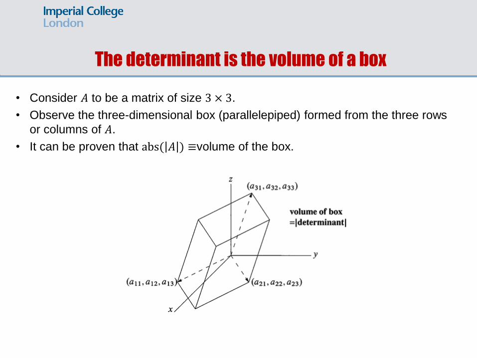
The determinant is the volume of a box

• Consider 𝐴 to be a matrix of size 3 × 3.

• Observe the three-dimensional box (parallelepiped) formed from the three rows

or columns of 𝐴.

• It can be proven that abs( 𝐴 ) ≡volume of the box.

det 𝐴 ≡volume of a box

• Take 𝐴 = 𝐼. Then the box mentioned previously is the unit cube and its volume

is 1.

Problem:

Consider an orthogonal square matrix 𝑄. Prove that det 𝑄 = 1 or −1.

Solution:

𝑄𝑇𝑄 = 𝐼 ⇒ det 𝑄𝑇𝑄 = det 𝑄𝑇 det 𝑄 = det (𝐼) = 1

But det 𝑄𝑇 =det 𝑄 ⇒ 𝑄 2 = 1 ⇒ 𝑄 = ±1

• The above results verifies also the fact that the determinant of a 3 × 3 matrix is

the volume of the cube that is formed by the rows of the matrix. This is because

if you consider 𝐴 = 𝑄 with 𝑄 being an orthogonal matrix, the related box is a

rotated version of the unit cube in the 3D space. Its volume is again 1.

• Take 𝑄 and double one of its vectors. The cube’s volume doubles (you have two

cubes sitting on top of each other.) The determinant doubles as well (property

3a).