Mathematics Meets Medicine: An Optimal Alignment · Mathematics Meets Medicine: An Optimal...

Mathematics Meets Medicine:An Optimal Alignment

Jan Modersitzki

Department of

Computing and Software

McMaster University

Hamilton, Canada

http://www.cas.mcmaster.ca/˜modersit

http://www.cas.mcmaster.ca/~modersit

Mathematics Meets Medicine c© Jan Modersitzki, March 28, 2008,

MotivationImage RegistrationGiven a reference image R and a template image T ,

find a reasonable transformation y, such that

the transformed image T [y] is similar to R

refe

renc

eR

tem

plat

eT

transformed template T [y]

A1 IR T D S 1 C F+R VP RIC Σ Titlepage Motivation Outline


MotivationImage RegistrationGiven a reference image R and a template image T ,

find a reasonable transformation y, such that

the transformed image T [y] is similar to RQuestions:

I What is a transformed image T [y]? image model T [y]

I What is similarity of T [y] and R? D[ T [y],R ]

I What is reasonability of y? S[ y ]

Image Registration: Variational Problem

D[ T [y],R ] + S[ y− yreg ]y−→ min, yreg(x) = x



OutlineI Applications

I Variational formulation D[ T [y],R ] + S[ y ]y−→ min

I image models T[y]I distance measures D[ T[y], R ]I regularizer S[ y ]

I Numerical methods

I Constrained image registration

I Conclusions



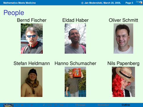
PeopleBernd Fischer Eldad Haber Oliver Schmitt

Stefan Heldmann Hanno Schumacher Nils Papenberg



Applications

A1 IR T D S 1 C F+R VP RIC Σ HNSP fMRI DTI Mam Liver Motion SPECT∑


HNSP: Sectioningwith Oliver Schmitt,Institute of Anatomy, University Rostock, Germany

I slicedI flattenedI stainedI mountedI . . .I digitized

large scale digital images, up to 10.000× 20.000 pixel



HNSP: Microscopy



HNSP: Deformed Imagessections 3.799 and 3.800 out of about 5.000

human affine linear elastic

|Torig − R| = 100% |Tlinear − R| = 72% |Telastic−R| = 50%



HNSP: Results3D elastic registration of a part of the visual cortex(two hemispheres; 100 sections a 512× 512 pixel)



Neuroimaging (fMRI)with Brian A. Wandell, Department of Psychology,Stanford Vision Science and Neuroimaging Group

“flattened visual cortex”



DTI: Diffusion Tensor Imagingwith Brian A. Wandell, Department of Psychology,Stanford Vision Science and Neuroimaging Group



MR-mammography, biopsy (open MR)with Bruce L. Daniel,Department of Radiology, Stanford University

pre contrast post contrast 3D



Virtual Surgery PlanningS. Bommersheim & N. Papenberg, SAFIR, BMBF/FUSIONFuture Environment for Gentle Liver Surgery Using Image-Guided Planning and Intra-Operative Navigation



Results for 3D US/CT

with Oliver Mahnke, SAFIR, University of Lubeck& MiE GmbH, Seth, Germany



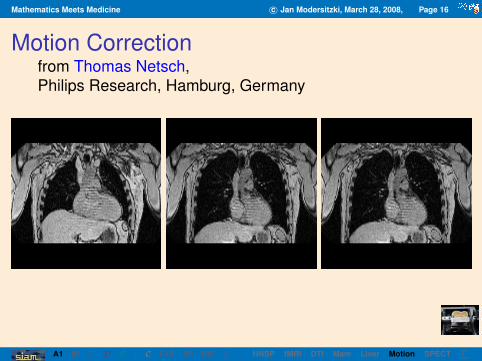
Motion Correctionfrom Thomas Netsch,Philips Research, Hamburg, Germany



SPECT: Single Photon Emissions CTwith Oliver Mahnke, SAFIR, University of Lubeck& MiE GmbH, Seth, Germany

image registered Lester



Registration in Medical ImagingI Comparing/merging/integrating images from different

I times, e.g., pre-/post surgery

I devices, e.g., CT-images/MRI

I perspectives, e.g., panorama imaging

I objects, e.g., atlas/patient mapping

I Template matching, e.g., catheter in blood vessel

I Atlas mapping, e.g., find 2D view in 3D data

I Serial sectioning, e.g., HNSP

I . . .

Registration is not restricted to medical applications



Classification of Registration TechniquesI feature spaceI search spaceI search strategyI distance measure

I dimensionality of images (d = 2, 3, 4, . . .)I modality (binary, gray, color, . . . )I mono-/multimodal imagesI acquisition (photography, FBS, CT, MRI, . . . )I inter/intra patient



Image Registration

A1 IR T D S 1 C F+R VP RIC Σ


Transforming Images

D[ T [y],R ] + αS [ y− yreg ]y−→ min

A1 IR T D S 1 C F+R VP RIC Σ I MS ML y


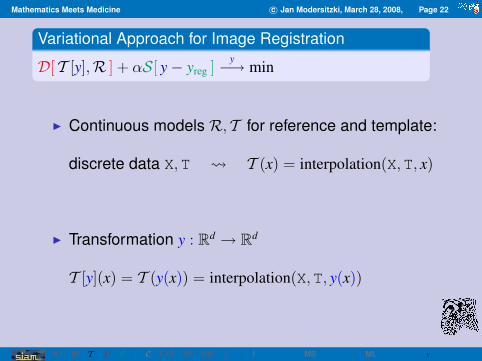
Variational Approach for Image Registration

D[ T [y],R ] + αS[ y− yreg ]y−→ min

I Continuous models R, T for reference and template:

discrete data X,T T (x) = interpolation(X,T, x)

I Transformation y : Rd → Rd

T [y](x) = T (y(x)) = interpolation(X,T, y(x))



Interpolation



Multi-Scale



Multilevel



Transforming Images

T [y](x) = T (y(x)) = interpolation(X,T, y(x))no

n-lin

ear



Distance Measures




Distance MeasuresI Feature Based

(Markers / Landmarks / Moments / Localizer)

I L2-norm, Sum of Squared Differences (SSD)

DSSD[ T [y],R ] = 12

∫Ω

[ T (y(x))−R(x) ]2 dx,

I correlation

I Mutual Information (multi-modal images)

I Normalized Gradient Fields

I . . .



Sum of Squared Differences



Mutual Information



Regularization


A1 IR T D S 1 C F+R VP RIC Σ Ill-Posed (Non-)Parametric Regularizer Square Σ


Transformation y

1 2 34 5 67 8

1 2 34 5 87 6

I Registration is severely ill-posed

I Restrictions onto the transformation y needed

I Goal: implicit physical restrictions



Implicit versus Explicit Regularization . . .Registration is ill-posed requires regularization

I Parametric RegistrationI restriction to (low-dimensional) space

(rigid, affine linear, spline,. . . )I regularized by properties of the space (implicit)I not physical or model based

I Non-parametric RegistrationI regularization by adding penalty or likelihood (explicit)I allows for a physical modelI y is no longer parameterizable



. . . implicit versus explicit regularization

registration is ill-posed requires regularization

I parametric registration

parametric registration

D[ R,T; y ]y= min s.t. y ∈ Q = x +

∑wjqj, w ∈ Rm

I non-parametric registration

non-parametric registration

D[ R,T; y ] + αS[ y− yreg ]y= min



References for Well-PosednessM. Droske and M. Rumpf.A variational approach to non-rigid morphological registration.SIAM Appl. Math., 64(2):668–687, 2004.

B. Fischer and J. Modersitzki.A unified approach to fast image registration and a new curvaturebased registration technique.Linear Algebra and its Applications, 380:107–124, 2004.

J. Weickert and C. Schnorr.A theoretical framework for convex regularizers in PDE-basedcomputation of image motion.Int. J. Computer Vision, 45(3):245–264, 2001.

. . .



Regularizer Sy(x) = x + u(x), displacement u : Rd → Rd

I “elastic registration” Selas[ u ] = elastic potential of u

I “fluid registration” Sfluid[ u ] = elastic potential of ∂tu

I “diffusion registration” Sdiff[ u ] = 12

∑d`=1

∫Ω‖∇u`‖2

R2 dx

I “curvature registration” Scurv[ u ] = 12

∑d`=1

∫Ω

(∆u`)2 dx

I . . .



Elastic RegistrationTransformation/displacement, y(x) = x + u(x)

Selas[ u ] = elastic potential of u

=

∫Ω

λ+ µ

2‖ ∇ · u‖2 +

µ

2

d∑i=1

‖ ∇ ui‖2 dx

image painted on a rubber sheet

C. Broit.Optimal Registration of Deformed Images.PhD thesis, University of Pensylvania, 1981.

Bajcsy & Kovacic 1986, Christensen 1994, Bro-Nielsen 1996,Gee et al. 1997, Fischer & M. 1999, Rumpf et al. 2002, . . .



Fluid RegistrationTransformation/displacement, y(x, t) = x + u(x, t)

Sfluid[ u ] = elastic potential of ∂tu

image painted on honey

GE. Christensen.Deformable Shape Models for Anatomy.PhD thesis, Sever Institute of Technology, Washington University,1994.

Bro-Nielsen 1996, Henn & Witsch 2002, . . .



Diffusion RegistrationTransformation/displacement, y(x) = x + u(x)

Sdiff[ u ] = oszillations of u= 1

2

∑d`=1

∫Ω‖∇u`‖2

R2 dx

heat equation

B. Fischer and J. Modersitzki.Fast diffusion registration.AMS Contemporary Mathematics, Inverse Problems, ImageAnalysis, and Medical Imaging, 313:117–129, 2002.

Horn & Schunck 1981, Thirion 1996, Droske, Rumpf & Schaller2003, . . .



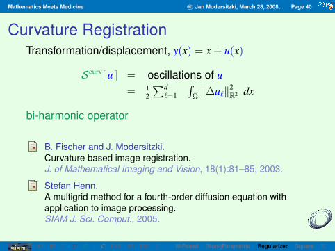
Curvature RegistrationTransformation/displacement, y(x) = x + u(x)

Scurv[ u ] = oscillations of u= 1

2

∑d`=1

∫Ω‖∆u`‖2

R2 dx

bi-harmonic operator

B. Fischer and J. Modersitzki.Curvature based image registration.J. of Mathematical Imaging and Vision, 18(1):81–85, 2003.

Stefan Henn.A multigrid method for a fourth-order diffusion equation withapplication to image processing.SIAM J. Sci. Comput., 2005.



Registration of a Curvature Registration

I Goal: do not penalize affine linear transformationsS[ Cx + b ]

!= 0 for all C ∈ Rd×d and b ∈ Rd

I But: Sdiff,elas,fluid,...[ Cx + b ] 6= 0 !

I Idea: Scurv[ y ] =∑

`

∫Ω

(∆y`)2 dx ⇒ Scurv[ Cx + b ] = 0

reference “fluid” “curvature”



Summary Regularization

I Registration is ill-posed requires regularization

I Regularizer controls reasonability of transformation

I Application conform regularization

I Enabling physical models(linear elasticity, fluid flow, . . . )

I high dimensional optimization problems



Numerical Methodsfor Image Registration

A1 IR T D S 1 C F+R VP RIC Σ OD DO ML Books


Optimize↔ DiscretizeImage Registration

D[ T [y],R ] + αS[ y− yreg ]y−→ min, yreg(x) = x

Numerical Approaches:

I Optimize→ Discretize

I Discretize→ Optimize

I relatively large problems:2.000.000 – 500.000.000 unknowns



Optimize→ Discretize: ELEImage Registration

J [y] = D[ T [y],R ] + αS[ y− yreg ]y−→ min, yreg(x) = x

I Euler-Lagrange eqs. (ELE) give necessary condition:Dy + αSy = 0 ⇐⇒ f [y] + αAy = 0system of non-linear partial differential eqs. (PDE)

I outer forces f , drive registration

I inner forces Ay, tissue properties

I ELE PDE: balance of forces



Optimize→ Discretize: SummaryContinuous Euler-Lagrange equations

f [y] + αA y = 0, f [yk] + αA yk+1 = 0, f [y] + αA y = yt

all difficulties dumped into right hand side fspatial discretization straightforwardefficient solvers for linear systemssmall controllable steps ( movies)moderate assumptions on f and A (smoothness)

no optimization problem behindnon-linearity only via fsmall stepssoftware: http://www.math.uni-luebeck.de/SAFIR


http://www.math.uni-luebeck.de/SAFIR


Discretize→ Optimize: SummaryDiscretization finite dimensional problem: yh ≈ y(xh)

D(yh) + αS(yh)yh

−→ min, yh ∈ Rn, h −→ 0

efficient optimization schemes (Newton-type)linear systems of type H δy = −rhs,

H = M + αB>B, M ≈ Dyy, rhs = Dy + α(B>B)yh

efficient multigrid solver for linear systemslarge steps

discretization not straightforward (multigrid)all parts have to be differentiable (data model)



Multilevel



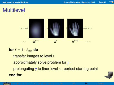
Multilevel

· · · → → → → · · ·

· · · h`−1 h` h`+1 · · ·

for ` = 1 : `max do

transfer images to level `

approximately solve problem for y

prolongating y to finer level perfect starting point

end for



Advantages of Multilevel Strategy

Regularization

Focus on essential minima

Creates extraordinary starting value

Reduces computation time

?



Example: Multilevel Iteration History



Literature

I Hajnal JV, Hill DLG, Hawkes DJ: Medical Image Registration, CRC 2001.

I Modersitzki J: Numerical Methods for Image Registration, OUP 2004.

I Goshtasby AA: 2-D and 3-D Image Registration, Wiley 2005.



Constrained Image Registration

A1 IR T D S 1 C F+R VP RIC Σ In


Example: COLDCombining Landmarks and Distance Measures

R T T [yLM] T [yCOLD]

Patent AZ 10253 784.4; Fischer & M., 2003

A1 IR T D S 1 C F+R VP RIC Σ In


Adding ConstraintsConstrained Image Registration

D[ T [y],R ] + αS[ y− yreg ] + β∫

Ωψ(Csoft[ y ]

)dx

y−→ min

subject to Chard[ y ](x) = 0 for all x ∈ ΩC

Example: landmarks/volume preservation

CLMi [ y ] = ‖y(ri)− ti‖, ψ(C) = 0.5‖C‖2

CVP[ y ](x) = det(∇y(x)), ψ(C) = (log C)2

I soft constraints (penalty)

I hard constraints

I both constraintsA1 IR T D S 1 C F+R VP RIC Σ In


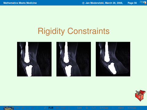
Rigidity Constraints

A1 IR T D S 1 C F+R VP RIC Σ Soft Q 1+1 S-Knee Σ Hard H-Knee Σ


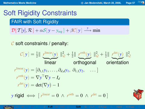
Soft Rigidity ConstraintsFAIR with Soft Rigidity

D[ T [y],R ] + αS[ y− yreg ] + βC[ y ]y−→ min

C soft constraints / penalty:

C[ y ] = 12‖ rlinear(y)︸︷︷︸

linear

‖2Q + 1

2‖ rorth(y)︸︷︷︸orthogonal

‖2Q + 1

2‖ rdet(y)︸︷︷︸orientation

‖2Q

rlinear(y) = [∂1,1y1, . . . , ∂d,dy1, ∂1,1y2, . . . ]

rorth(y) = ∇y>∇y− Id

rdet(y) = det(∇y)− 1

y rigid ⇐⇒ [ rlinear = 0 ∧ rorth = 0 ∧ rdet = 0 ]



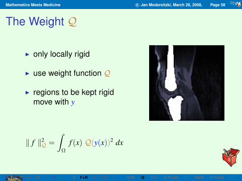
The Weight Q

I only locally rigid

I use weight function Q

I regions to be kept rigidmove with y

‖ f ‖2Q =

∫Ω

f (x) Q(y(x))2 dx



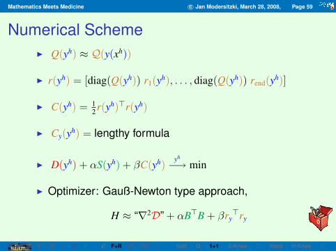
Numerical SchemeI Q(yh) ≈ Q(y(xh))

I r(yh) = [diag(Q(yh)) r1(yh), . . . , diag(Q(yh)) rend(yh)]

I C(yh) = 12r(yh)>r(yh)

I Cy(yh) = lengthy formula

I D(yh) + αS(yh) + βC(yh)yh

−→ min

I Optimizer: Gauß-Newton type approach,

H ≈ “∇2D” + αB>B + βry>ry



Example: KneeT & grid det(∇y)− 1 T(y)

notp

enal

ized

pena

lized



Summary of Soft Rigidity Constraints

Results are OK

Implementation is straightforward

Constraints are not fulfilled

How to pick penalty (β, ψ)?



Hard Rigidity ConstraintsFAIR with Hard Rigidity

D[ T [y],R ]+αS[ y− yreg ]y−→ min subject to y rigid onQ

Eulerian→ Lagrangiancomputations of D and Sinvolve det(∇y)

rigidity in T domain “linear” constraints

y(x) = Dkx+tk, k = 1 : #segments



Lagrangian Model of Rigidity (2D)I rigid on segment i

y(x) = Q(x)wi =

(cos wi

1 − sin wi1

sin wi1 cos wi

1

)(x1

x2

)+

(wi

2wi

3

)I w = (w1, . . . ,wm), C = (C1, . . . , Cm), m = #segments

C i[ y,w ] = y(x)− Q(x)wi, i = 1, . . . ,m

I Lagrangian:

L(y,w, p) = D[ y ] + αS[ y ] + p>C[ y,w ]

I Numerical Scheme:

Sequential Quadratic Programming



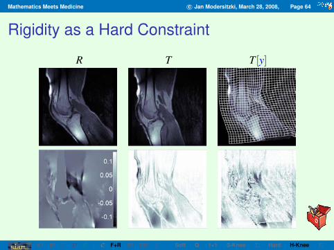
Rigidity as a Hard Constraint

R T T[y]



Summary of Hard Rigidity Constraints

Results are OK

Implementation is interesting

Constraints are fulfilled

No additional Parameters



Volume Preserving ImageRegistration

A1 IR T D S 1 C F+R VP RIC Σ In Soft Hard Dis Opt Blobs MRI


Example: Tumor MonitoringMRI scans of a female breast, with Bruce L. DanielDepartment of Radiology, Stanford University

pre

cont

rast

post

cont

rast

pre

cont

rast

post

cont

rast



Volume Preserving Constraints

∫y(V)

dx =

∫V

dx for all V ⊂ Ω

assuming y to be sufficient smooth,

det(∇y) = 1 for all x ∈ Ω

Volume Preserving Constraints

C[ y ](x) = det(∇y(x))− 1, x ∈ ΩC



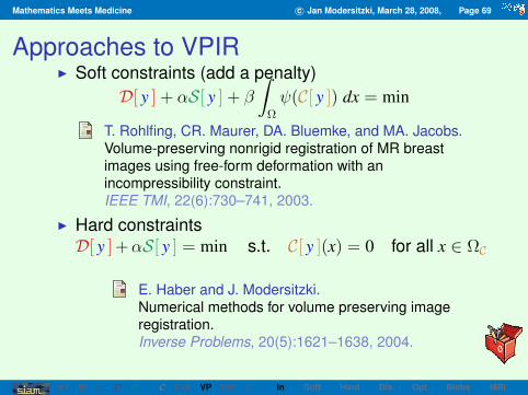
Approaches to VPIRI Soft constraints (add a penalty)

D[ y ] + αS[ y ] + β

∫Ω

ψ(C[ y ]) dx = min

T. Rohlfing, CR. Maurer, DA. Bluemke, and MA. Jacobs.Volume-preserving nonrigid registration of MR breastimages using free-form deformation with anincompressibility constraint.IEEE TMI, 22(6):730–741, 2003.

I Hard constraintsD[ y ] +αS[ y ] = min s.t. C[ y ](x) = 0 for all x ∈ ΩC

E. Haber and J. Modersitzki.Numerical methods for volume preserving imageregistration.Inverse Problems, 20(5):1621–1638, 2004.

I Mass preservationS. Haker and A. Tannenbaum.Optimal transport and image warping.MICCAI 2001, pages 120–127, 2001.

L. Zhu, S. Haker, and A. Tannenbaum.Area preserving mappings for the visulization of medicalstructures.MICCAI 2003, pages 277–284, 2003.



Volume Preservation using Soft Constraints

D[ y ] + αS[ y ] + β

∫Ω

log2 (Csoft[ y ] + 1)

dxy−→ min

Drawbacks of Soft Constraints

I constraints are generally not fulfilled

I small soft constraints might be large on small regions(tumor!)

I additional parameters

I bad numerics for β →∞



Continuous Framework, Hard ConstraintsVPIR

D[ y ] + αS[ y ]y−→ min s.t. C[ y ] = 0, x ∈ ΩC

I Distance measure D with Gateaux derivative

dy,vD[ y ] =∫

Ω〈f (x, y(x)), v(x)〉Rd dx

I Regularizer S with Gateaux derivative

dy,vS[ y ] =∫

Ω〈By(x),Bv(x)〉Rd dx

I Volume preserving constraints

C[ u ] = det(∇y)− 1dy,vC[ y ] = det(∇y)

⟨∇y−>,∇v

⟩Rd,d



Example: Volume Preservation in 2D

C[ x + u(x) ] = det(I2 +∇u)− 1= ∂1u1 + ∂2u2 + ∂1u1∂2u2 − ∂2u1∂1u2

= ∇ · u + N[u]

I N is nonlinear, N[0] = 0I linearization

Cy ≈ ∇ · + [ξ(x) · ∂1 η(x) · ∂2]

I Stokes problem, needs careful discretization tokeep LBB conditions or h-ellipticity



Discretizing . . .I T and R on cell center gridI y = [y1, y2] on staggered grids

•

•

•

•

•

•

•

•

•

I

I

I

I

I

I

I

I

I

I

I

I

N N N

N N N

N N N

N N N

N

N

I

I

I vol(V, y) =∫

y(V)dx ≈ vol(box), ci = vol(boxi)− hd

I C(yh) = (ci)ni=1, Cy(yh) straightforward but lengthy



. . . and OptimizeDiscrete VPIRFind yh such that

D(yh)+αS(yh)yh

−→ min s.t. Ci(yh) = 0, i = 1 : #voxel

I SQP: Sequential Quadratic ProgrammingI Lagrangian with multiplier p

L(yh, p) = D(yh) + αS(yh) + p>C(yh)

I Necessary conditions for a minimizer: ∇L(yh, p) = 0I Gauß-Newton type method, H = “∇2D” + αB>B(

H CyCy> 0

)(δyδp

)= −

(Ly

Lp

)



Details . . .

I Solving the KKT system: MINRES(H Cy

Cy> 0

)(δyδp

)= −

(Ly

Lp

)

I with preconditioner(H

S

),

S ≈ Cy H−1 Cy>

S−1 := Cy† H (Cy

†)>

Cy† = (Cy Cy

>)−1Cy

I Multigrid for H and Cy Cy>



. . . detailsI Line search for yh ← yh + γδyh based on merit function

meritKKT(yh) := D(yh) + αS(yh) + θ‖C(yh)‖1

θ := ‖p‖∞ + θmin

p from ‖Dy + αSy + Cy>p‖ p−→ min

note, (Cy Cy>)p = −Cy(Dy + αSy)

I For the projection step:

meritC(yh) := ‖C(yh)‖22

I If meritC(yh) > tol, solve for correction δy such that

C(yh + δy) ≈ C(yh) + Cy(yh) δy = 0

I Assuming Cy has full rank,

δy = Cy> w, where (Cy Cy

>) w = −C(yh)



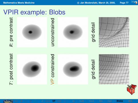
VPIR example: BlobsR

:pr

eco

ntra

st

unco

nstra

ined

grid

deta

il

T:

post

cont

rast

VP

cons

train

ed

grid

deta

il



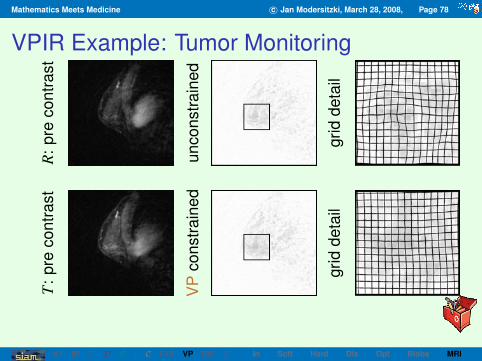
VPIR Example: Tumor MonitoringR

:pr

eco

ntra

st

unco

nstr a

ined

grid

deta

il

T:

pre

cont

rast

VP

cons

train

ed

grid

deta

ilA1 IR T D S 1 C F+R VP RIC Σ In Soft Hard Dis Opt Blobs MRI


VPIR Example: Tumor Monitoring

unconstrained VP constrained



Registration and IntensityCorrection

A1 IR T D S 1 C F+R VP RIC Σ In RIC MRI NSP


Distance MeasuresI images features (moments, landmarks, markers, . . . )I sum of squared differences (SSD)I mutual information (MI)

Problem: sophisticated distance measures enableregistration, but do not correct intensities

R T |T − R|

http://www.sci.utah.edu/stories/2002/sum mri-epi.htmlA1 IR T D S 1 C F+R VP RIC Σ In RIC MRI NSP


RIC: Registration and Intensity CorrectionRegistration and Intensity Correction

J [y, s] = D[ T [y], s R ] + S[ y− yreg ] + Hom(s)y,s−→ min

D[ T [y], s R ]e.g.= 1

2‖T [y]−sR‖2L2

= 12

∫ (T (y(x))−s(x)R(x)

)2dx

intensity correction needs to be regularized(excludes trivial solutions s = T /R, s ≡ 1)

choices: Hom(s) =∫|∇s|p dx, |∇s| =

√(∂1s)2 + (∂2s)2

I diffusivity for p = 2I total variation for p = 1I Mumford-Shah penaltyI . . .A1 IR T D S 1 C F+R VP RIC Σ In RIC MRI NSP


MRI inhomogeneitiesImages from Samsonov, Whitaker, & Johnson, University of Utah

R T(yRIC) TV correction s

s R |T(yRIC)− s R| |T(yplain)− R|



Staining ArtifactsImages from Oliver Schmitt, Anatomy, University Rostock

R T(yRIC) TV correction s

s R |T(yRIC)− s R| |T(yplain)− R|



Summary



SummaryI Introduction to image registration:

important, challenging, interdisciplinary

I General framework based on a variational approach:D[ T [y],R ] + αS[ y− yreg ]

y−→ min

I Discussion of various building blocks:I image model T [y]I distance measures DI regularizer S

I Numerical methods:multilevel, optimize↔ discretize

I Constraints C:landmarks, local rigidity, intensity correction, . . .



Solutions and Algorithms For Image Registration


Mathematics Meets Medicine: An Optimal Alignment · Mathematics Meets Medicine: An Optimal...

Documents

Transcript of Mathematics Meets Medicine: An Optimal Alignment · Mathematics Meets Medicine: An Optimal...