1

Mathematics Applications is an ATAR course which focuses on the use of mathematics to solve problems in contexts that involve financial modelling,

geometric and trigonometric analysis, graphical and network analysis, and growth and decay in sequences. It also provides opportunities for students to

develop systematic strategies based on the statistical investigation process for answering questions that involve analysing univariate and bivariate data,

including time series data.

Text: Sadler Applications Unit 3 and 4

Week Syllabus Reference Sadler Reference Assessment

1-2 Topic 3.1: Bivariate data analysis (20 hours)

The statistical investigation process

3.1.1 review the statistical investigation process: identify a problem; pose a statistical

question; collect or obtain data; analyse data; interpret and communicate results

Identifying and describing associations between two categorical variables

3.1.2 construct two-way frequency tables and determine the associated row and column

sums and percentages

3.1.3 use an appropriately percentaged two-way frequency table to identify patterns that

suggest the presence of an association

3.1.4 describe an association in terms of differences observed in percentages across

categories in a systematic and concise manner, and interpret this in the context of the

data

Unit 3 Chapter 1 Ex 1A

MATHEMATICS LEARNING AREA

Mathematics Applications Units 3 and 4

Course Outline

2

Identifying and describing associations between two numerical variables

3.1.5 construct a scatterplot to identify patterns in the data suggesting the presence of an

association

3.1.6 describe an association between two numerical variables in terms of direction

(positive/negative), form (linear/non-linear) and strength (strong/moderate/weak)

3.1.7 calculate, using technology, and interpret the correlation coefficient (r) to quantify

the strength of a linear association

Unit 3 Chapter 1 Exercise 1B

2-3

Fitting a linear model to numerical data

3.1.8 identify the response variable and the explanatory variable for primary and

secondary data

3.1.9 use a scatterplot to identify the nature of the relationship between variables

3.1.10 model a linear relationship by fitting a least-squares line to the data

3.1.11 use a residual plot to assess the appropriateness of fitting a linear model to the data

3.1.12 interpret the intercept and slope of the fitted line

3.1.13 use the coefficient of determination to assess the strength of a linear association in

terms of the explained variation

3.1.14 use the equation of a fitted line to make predictions

3.1.15 distinguish between interpolation and extrapolation when using the fitted line to

make predictions, recognising the potential dangers of extrapolation

3.1.16 write up the results of the above analysis in a systematic and concise manner

Unit 3 Chapter 1 Exercise 1C, 2A

Investigation 1

4-5

Association and causation

3.1.17 recognise that an observed association between two variables does not necessarily

mean that there is a causal relationship between them

3.1.18 identify possible non-causal explanations for an association, including coincidence and

confounding due to a common response to another variable, and communicate these

explanations in a systematic and concise manner

Unit 3 Chapter 2 Exercise 2B, 2C

3

The data investigation process

3.1.19 implement the statistical investigation process to answer questions that involve

identifying, analysing and describing associations between two categorical variables

or between two numerical variables

6-7 Topic 3.2: Growth and decay in sequences (15 hours)

The arithmetic sequence

3.2.1 use recursion to generate an arithmetic sequence

3.2.2 display the terms of an arithmetic sequence in both tabular and graphical form

and demonstrate that arithmetic sequences can be used to model linear growth

and decay in discrete situations

3.2.3 deduce a rule for the term of a particular arithmetic sequence from the

pattern of the terms in an arithmetic sequence, and use this rule to make

predictions

3.2.4 use arithmetic sequences to model and analyse practical situations involving

linear growth or decay

Unit 3 Chapter 3, Exercise 3A, 3B, 3C

8-9

The geometric sequence

3.2.5 use recursion to generate a geometric sequence

3.2.6 display the terms of a geometric sequence in both tabular and graphical form

and demonstrate that geometric sequences can be used to model exponential

growth and decay in discrete situations

3.2.7 deduce a rule for the term of a particular geometric sequence from the

pattern of the terms in the sequence, and use this rule to make predictions

3.2.8 use geometric sequences to model and analyse (numerically, or graphically

only) practical problems involving geometric growth and decay

Unit 3 Chapter 4 Exercise 4A, 4B

Test 1

4

10-11

Sequences generated by first-order linear recurrence relations

3.2.9 use a general first-order linear recurrence relation to generate the terms of a

sequence and to display it in both tabular and graphical form

3.2.10 generate a sequence defined by a first-order linear recurrence relation that gives

long term increasing, decreasing or steady-state solutions

3.2.11 use first-order linear recurrence relations to model and analyse (numerically or

graphically only) practical problems

Unit 3 Chapter 4 Exercise 4C

12-13 Topic 3.3: Graphs and networks (20 hours)

The definition of a graph and associated terminology

3.3.1 demonstrate the meanings of, and use, the terms: graph, edge, vertex, loop,

degree of a vertex, subgraph, simple graph, complete graph, bipartite graph,

directed graph (digraph), arc, weighted graph, and network

3.3.2 identify practical situations that can be represented by a network, and construct

such networks

3.3.3 construct an adjacency matrix from a given graph or digraph and use the matrix

to solve associated problems

Unit 3 Chapter 5 Exercise 5A, 5B

14

Planar graphs

3.3.4 demonstrate the meanings of, and use, the terms: planar graph and face

3.3.5 apply Euler’s formula, to solve problems relating to planar graphs.

Unit 3 Chapter 5 Exercise 5C

15

Paths and cycles

3.3.6 demonstrate the meanings of, and use, the terms: walk, trail, path, closed walk,

closed trail, cycle, connected graph, and bridge

3.3.7 investigate and solve practical problems to determine the shortest path between

two vertices in a weighted graph (by trial-and-error methods only)

Unit 3 Chapter 5 Exercise 5D, 5E

5

3.3.8 demonstrate the meanings of, and use, the terms: Eulerian graph, Eulerian trail,

semi-Eulerian graph, semi-Eulerian trail and the conditions for their existence,

and use these concepts to investigate and solve practical problems

3.3.9 demonstrate the meanings of, and use, the terms: Hamiltonian graph and semi-

Hamiltonian graph, and use these concepts to investigate and solve practical

problems

16 Shortest Path A systematic approach Semester 1 Examination Revision

Unit 3 Chapter 6 Exercise 6

Test 2

17

Semester 1 Examination

Semester 1 Examination

18 Topic 4.1: Time series analysis (15 hours)

Describing and interpreting patterns in time series data

4.1.1 construct time series plots

4.1.2 describe time series plots by identifying features such as trend (long term

direction), seasonality (systematic, calendar-related movements), and irregular

fluctuations (unsystematic, short term fluctuations), and recognise when there

are outliers

Unit 4 Chapter 1 Exercise 1A

Investigation 2

19

Analysing time series data

4.1.3 smooth time series data by using a simple moving average, including the use of

spreadsheets to implement this process

4.1.4 calculate seasonal indices by using the average percentage method

Unit 4 Chapter 2 Exercise 2A, 2B

6

4.1.5 deseasonalise a time series by using a seasonal index, including the use of

spreadsheets to implement this process to fit a least-squares line to model long-

term trends in time series data

4.1.7 predict from regression lines, making seasonal adjustments for periodic data

The data investigation process

4.1.8 implement the statistical investigation process to answer questions that involve

the analysis of time series data

Exercise 2C, 2D

20 Topic 4.2: Loans, investments and annuities (20 hours)

Compound interest loans and investments

4.2.1 use a recurrence relation to model a compound interest loan or investment and

investigate (numerically or graphically) the effect of the interest rate and the

number of compounding periods on the future value of the loan or investment

4.2.2 calculate the effective annual rate of interest and use the results to compare

investment returns and cost of loans when interest is paid or charged daily,

monthly, quarterly or six-monthly

4.2.3 with the aid of a calculator or computer-based financial software, solve

problems involving compound interest loans, investments and depreciating

assets

Unit 4 Chapter 3 Exercise 3A,

21-22

Reducing balance loans (compound interest loans with periodic repayments)

4.2.4 use a recurrence relation to model a reducing balance loan and investigate

(numerically or graphically) the effect of the interest rate and repayment amount

on the time taken to repay the loan

4.2.5 with the aid of a financial calculator or computer-based financial software,

solve problems involving reducing balance loans

Unit 4 Chapter 3 Exercise 3B, 3C, 3D

7

23-24

Annuities and perpetuities (compound interest investments with periodic payments made

from the investment)

4.2.6 use a recurrence relation to model an annuity, and investigate (numerically or

graphically) the effect of the amount invested, the interest rate, and the payment

amount on the duration of the annuity

4.2.7 with the aid of a financial calculator or computer-based financial software, solve

problems involving annuities (including perpetuities as a special case)

Unit 4 Chapter 3 Exercise 3D, 3E, Chapter 4 Exercise 4A, 4B

Investigation 3

25 Topic 4.3: Networks and decision mathematics (20 hours)

Trees and minimum connector problems

4.3.1 identify practical examples that can be represented by trees and spanning trees

4.3.2 identify a minimum spanning tree in a weighted connected graph, either by

inspection or by using Prim’s algorithm

4.3.3 use minimal spanning trees to solve minimal connector problems

Unit 4 Chapter 5 Exercise 5A, 5B Chapter 6 Exercise 6A, 6B

Test 3

26

Project planning and scheduling using critical path analysis (CPA)

4.3.4 construct a network to represent the durations and interdependencies of

activities that must be completed during the project

4.3.5 use forward and backward scanning to determine the earliest starting time (EST)

and latest starting times (LST) for each activity in the project

4.3.6 use ESTs and LSTs to locate the critical path(s) for the project

4.3.7 use the critical path to determine the minimum time for a project to be

completed

4.3.8 calculate float times for non-critical activities

Unit 4 Chapter 7 Exercise 7A, 7B

8

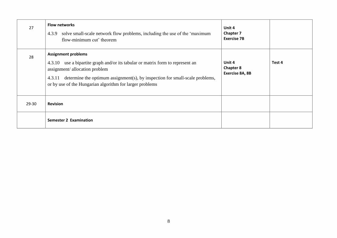
27

Flow networks

4.3.9 solve small-scale network flow problems, including the use of the ‘maximum

flow-minimum cut’ theorem

Unit 4 Chapter 7 Exercise 7B

28

Assignment problems

4.3.10 use a bipartite graph and/or its tabular or matrix form to represent an

assignment/ allocation problem

4.3.11 determine the optimum assignment(s), by inspection for small-scale problems,

or by use of the Hungarian algorithm for larger problems

Unit 4 Chapter 8 Exercise 8A, 8B

Test 4

29-30

Revision

Semester 2 Examination

9

2017 Assessment Record – Mathematics Applications Year 12- Unit 3 and 4

Assessment My Raw mark (%) YEAR Weighting YEAR Value (Raw mark x

weighting) Test 1

8 %

Test 2

8 %

Test 3

12 %

Test 4

12 %

Investigation 1 6

3

2%

Investigation 2 6

3

2%

Investigation 3 6

3

2%

Semester 1 EXAM

15%

Semester 2 EXAM – 25%

ASSESSMENT PROCEDURE 2017

Refer to College Diary