Mathematics and Statistics in...

UsingBioInteractiveResourcestoTeachMathematicsandStatisticsinBiology Pg.1

UsingBioInteractive

ResourcestoTeach

Mathematicsand

Statisticsin

Biology

PaulStrode,PhDFairviewHighSchoolBoulder,Colorado

AnnBrokawRockyRiverHighSchool

RockyRiver,Ohio

Version:October2015

2015


UsingBioInteractiveResourcestoTeach

MathematicsandStatisticsinBiologyAboutThisGuide 3 StatisticalSymbolsandEquations 4

Part1:DescriptiveStatisticsUsedinBiology 5MeasuresofAverage:Mean,Median,andMode 7

Mean 7 Median 8 Mode 9 WhentoUseWhichOne 9 MeasuresofVariability:Range,StandardDeviation,andVariance 9 Range 9 StandardDeviationandVariance 10 UnderstandingDegreesofFreedom 12 MeasuresofConfidence:StandardErroroftheMeanand95%ConfidenceInterval 13Part2:InferentialStatisticsUsedinBiology 17 SignificanceTesting:Theα(Alpha)Level 17 ComparingAverages:TheStudent’st-TestforIndependentSamples 18

AnalyzingFrequencies:TheChi-SquareTest 21 MeasuringCorrelationsandAnalyzingLinearRegression 25Part3:CommonlyUsedCalculationsinBiology 31 RelativeFrequency 31

Probability 31 RateCalculations 33 Hardy-WeinbergFrequencyCalculations 34 StandardCurves 36Part4:BioInteractive’sMathematicsandStatisticsClassroomResources 39 BioInteractiveResourceName(LinkstoClassroom-ReadyResources) 39


AboutThisGuideManystatesciencestandardsencouragetheuseofmathematicsandstatisticsinbiologyeducation,includingthenewlydesignedAPBiologycourse,IBBiology,NextGenerationScienceStandards,andtheCommonCore.SeveralresourcesontheBioInteractivewebsite(www.biointeractive.org),whicharelistedinthetableattheendofthisdocument,makeuseofmathandstatisticstoanalyzeresearchdata.Thisguideismeanttohelp

educatorsusetheseBioInteractiveresourcesintheclassroombyprovidingfurtherbackgroundonthe

statisticaltestsusedandstep-by-stepinstructionsfordoingthecalculations.Althoughmostoftheexampledatasetsincludedinthisguidearenotrealandaresimplyprovidedtoillustratehowthecalculationsaredone,thedatasetsonwhichtheBioInteractiveresourcesarebasedrepresentactualresearchdata.

Thisguideisnotmeanttobeatextbookonstatistics;itonlycoverstopicsmostrelevanttohighschoolbiology,focusingonmethodsandexamplesratherthantheory.Itisorganizedinfourparts:

• Part1coversdescriptivestatistics,methodsusedtoorganize,summarize,anddescribequantifiable

data.Themethodsincludewaystodescribethetypicaloraveragevalueofthedataandthespreadofthedata.

• Part2coversstatisticalmethodsusedtodrawinferencesaboutpopulationsonthebasisof

observationsmadeonsmallersamplesorgroupsofthepopulation—abranchofstatisticsknownasinferentialstatistics.

• Part3describesothermathematicalmethodscommonlytaughtinhighschoolbiology,including

frequencyandratecalculations,Hardy-Weinbergcalculations,probability,andstandardcurves.

• Part4providesachartofactivitiesontheBioInteractivewebsitethatusemathandstatisticsmethods.AfirstdraftoftheguidewaspublishedinJuly2014.Ithasbeenrevisedbasedonuserfeedbackandexpertreview,andthisversionwaspublishedinOctober2015.Theguidewillcontinuetobeupdatedwithnewcontentandbasedonongoingfeedbackandreview.

Foramorecomprehensivediscussionofstatisticalmethodsandadditionalclassroomexamples,refertoJohnMcDonald’sHandbookofBiologicalStatistics,http://www.biostathandbook.com,andtheCollegeBoard’sAPBiologyQuantitativeSkills:AGuideforTeachers,http://apcentral.collegeboard.com/apc/public/repository/AP_Bio_Quantitative_Skills_Guide-2012.pdf.


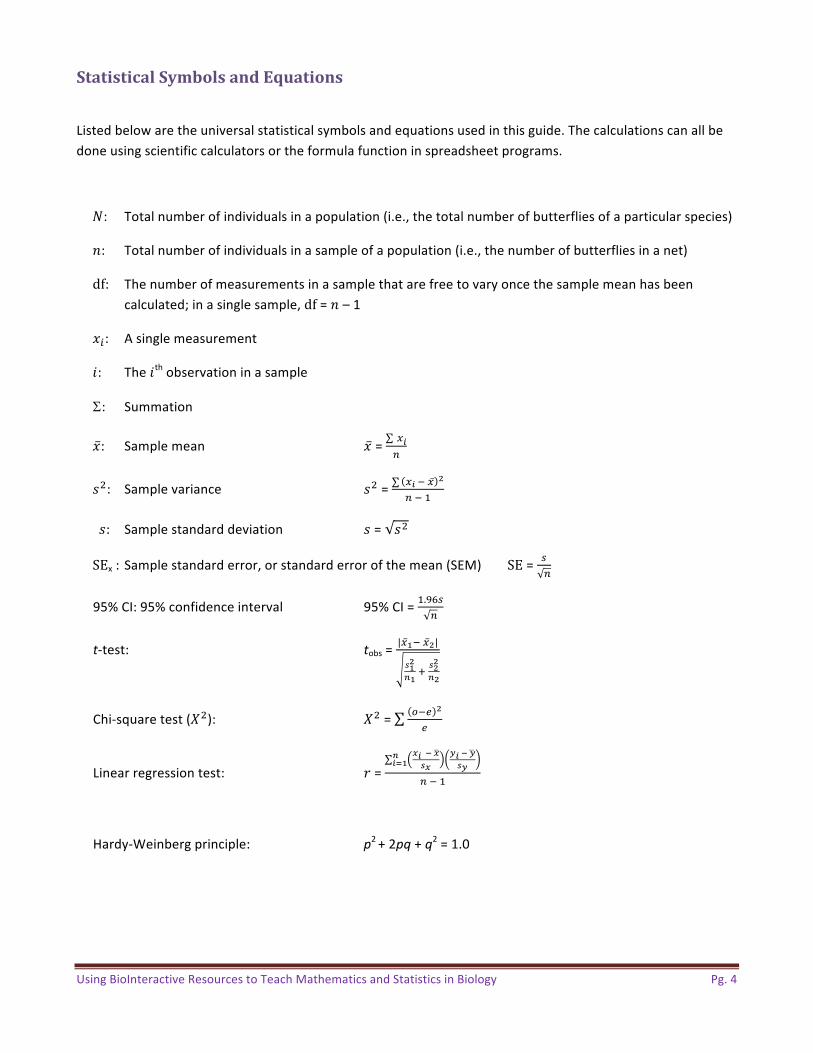
StatisticalSymbolsandEquations

Listedbelowaretheuniversalstatisticalsymbolsandequationsusedinthisguide.Thecalculationscanallbedoneusingscientificcalculatorsortheformulafunctioninspreadsheetprograms.

!: Totalnumberofindividualsinapopulation(i.e.,thetotalnumberofbutterfliesofaparticularspecies)

#: Totalnumberofindividualsinasampleofapopulation(i.e.,thenumberofbutterfliesinanet)

df: Thenumberofmeasurementsinasamplethatarefreetovaryoncethesamplemeanhasbeencalculated;inasinglesample,df=#–1

&': Asinglemeasurement

(: The(thobservationinasample

S: Summation

&: Samplemean &= *+,

-.: Samplevariance -.=∑ *+0*1

,02

-: Samplestandarddeviation -= -.

SEx: Samplestandarderror,orstandarderrorofthemean(SEM) SE= 5,

95%CI:95%confidenceinterval 95%CI=2.785,

t-test: tobs=|*:0*1|

;:1<:=;1

1<1

Chi-squaretest(>.): >.= ?0@ 1

@

Linearregressiontest: A=B+CB;B

<+D:

E+CE;E

,02

Hardy-Weinbergprinciple: p2+2pq+q2=1.0


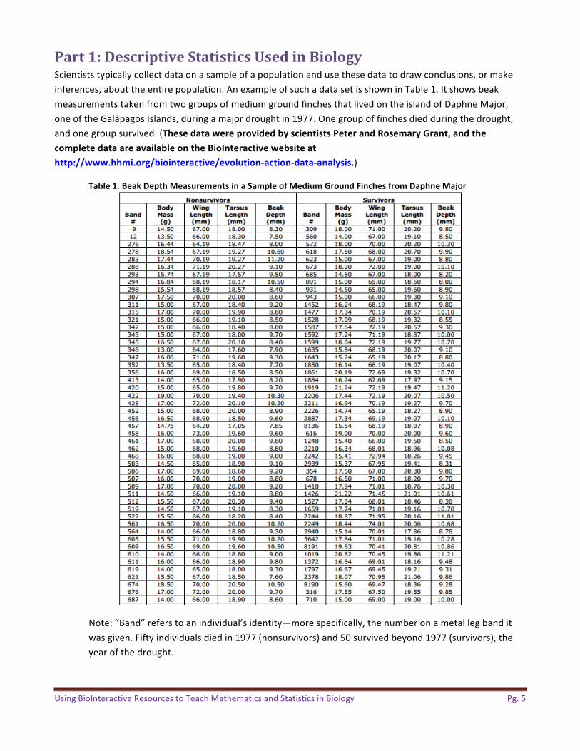
Part1:DescriptiveStatisticsUsedinBiologyScientiststypicallycollectdataonasampleofapopulationandusethesedatatodrawconclusions,ormakeinferences,abouttheentirepopulation.AnexampleofsuchadatasetisshowninTable1.ItshowsbeakmeasurementstakenfromtwogroupsofmediumgroundfinchesthatlivedontheislandofDaphneMajor,oneoftheGalápagosIslands,duringamajordroughtin1977.Onegroupoffinchesdiedduringthedrought,andonegroupsurvived.(ThesedatawereprovidedbyscientistsPeterandRosemaryGrant,andthe

completedataareavailableontheBioInteractivewebsiteat

http://www.hhmi.org/biointeractive/evolution-action-data-analysis.)

Table1.BeakDepthMeasurementsinaSampleofMediumGroundFinchesfromDaphneMajor

Note:“Band”referstoanindividual’sidentity—morespecifically,thenumberonametallegbanditwasgiven.Fiftyindividualsdiedin1977(nonsurvivors)and50survivedbeyond1977(survivors),theyearofthedrought.


HowwouldyoudescribethedatainTable1,andwhatdoesittellyouaboutthepopulationsofmediumgroundfinchesofDaphneMajor?Thesearedifficultquestionstoanswerbylookingatatableofnumbers.

OneofthefirststepsinanalyzingasmalldatasetliketheoneshowninTable1istographthedataand

examinethedistribution.Figure1showstwographsofbeakmeasurements.Thegraphonthetopshowsbeakmeasurementsoffinchesthatdiedduringthedrought.Thegraphonthebottomshowsbeakmeasurementsoffinchesthatsurvivedthedrought.

Beak Depths of 50 Medium Ground Finches That Did Not Survive the Drought

Beak Depths of 50 Medium Ground Finches That Survived the Drought

Figure1.DistributionsofBeakDepthMeasurementsinTwoGroupsofMediumGroundFinches

Noticethatthemeasurementstendtobemoreorlesssymmetricallydistributedacrossarange,withmostmeasurementsaroundthecenterofthedistribution.Thisisacharacteristicofanormaldistribution.Moststatisticalmethodscoveredinthisguideapplytodatathatarenormallydistributed,likethebeakmeasurementsabove;othertypesofdistributionsrequireeitherdifferentkindsofstatisticsortransformingdatatomakethemnormallydistributed.

Howwouldyoudescribethesetwographs?Howaretheythesameordifferent?Descriptivestatisticsallowsyoutodescribeandquantifythesedifferences.TherestofPart1ofthisguideprovidesstep-by-stepinstructionsforcalculatingmean,standarddeviation,standarderror,andotherdescriptivestatistics.


MeasuresofAverage:Mean,Median,andModeInthetwographsinFigure1,thecenterandspreadofeachdistributionisdifferent.Thecenterofthedistributioncanbedescribedbythemean,median,ormode.Thesearereferredtoasmeasuresofcentral

tendency.

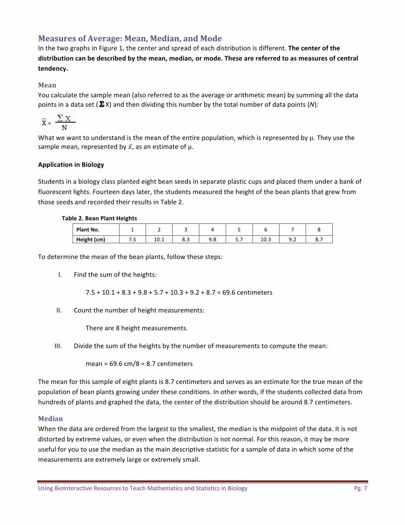
MeanYoucalculatethesamplemean(alsoreferredtoastheaverageorarithmeticmean)bysummingallthedatapointsinadataset(�X)andthendividingthisnumberbythetotalnumberofdatapoints(N):

Whatwewanttounderstandisthemeanoftheentirepopulation,whichisrepresentedbyµ.Theyusethesamplemean,representedby&,asanestimateofµ.

ApplicationinBiology

Studentsinabiologyclassplantedeightbeanseedsinseparateplasticcupsandplacedthemunderabankoffluorescentlights.Fourteendayslater,thestudentsmeasuredtheheightofthebeanplantsthatgrewfromthoseseedsandrecordedtheirresultsinTable2.

Table2.BeanPlantHeights

PlantNo. 1 2 3 4 5 6 7 8

Height(cm) 7.5 10.1 8.3 9.8 5.7 10.3 9.2 8.7Todeterminethemeanofthebeanplants,followthesesteps:

I. Findthesumoftheheights:

7.5+10.1+8.3+9.8+5.7+10.3+9.2+8.7=69.6centimeters

II. Countthenumberofheightmeasurements:Thereare8heightmeasurements.

III. Dividethesumoftheheightsbythenumberofmeasurementstocomputethemean:

mean=69.6cm/8=8.7centimeters

Themeanforthissampleofeightplantsis8.7centimetersandservesasanestimateforthetruemeanofthepopulationofbeanplantsgrowingundertheseconditions.Inotherwords,ifthestudentscollecteddatafromhundredsofplantsandgraphedthedata,thecenterofthedistributionshouldbearound8.7centimeters.

MedianWhenthedataareorderedfromthelargesttothesmallest,themedianisthemidpointofthedata.Itisnotdistortedbyextremevalues,orevenwhenthedistributionisnotnormal.Forthisreason,itmaybemoreusefulforyoutousethemedianasthemaindescriptivestatisticforasampleofdatainwhichsomeofthemeasurementsareextremelylargeorextremelysmall.


Todeterminethemedianofasetofvalues,youfirstarrangetheminnumericalorderfromlowesttohighest.Themiddlevalueinthelististhemedian.Ifthereisanevennumberofvaluesinthelist,thenthemedianisthemeanofthemiddletwovalues.


AresearcherstudyingmousebehaviorrecordedinTable3thetime(inseconds)ittook13differentmicetolocatefoodinamaze.

Table3.LengthofTimeforMicetoLocateFoodinaMaze

MouseNo. 1 2 3 4 5 6 7 8 9 10 11 12 13

Time(sec.) 31 33 163 33 28 29 33 27 27 34 35 28 32Todeterminethemediantimethatthemicespentsearchingforfood,followthesesteps:

I. Arrangethetimevaluesinnumericalorderfromlowesttohighest:

27,27,28,28,29,31,32,33,33,33,34,35,163

II. Findthemiddlevalue.Thisvalueisthemedian:

median=32secondsInthiscase,themedianis32seconds,butthemeanis41seconds,whichislongerthanallbutoneofthemicetooktosearchforfood.Inthiscase,themeanwouldnotbeagoodmeasureofcentraltendencyunlessthereallyslowmouseisexcludedfromthedataset.

ModeThemodeisanothermeasureoftheaverage.Itisthevaluethatappearsmostofteninasampleofdata.IntheexampleshowninTable3,themodeis33seconds.

Themodeisnottypicallyusedasameasureofcentraltendencyinbiologicalresearch,butitcanbeusefulindescribingsomedistributions.Forexample,Figure2showsadistributionofbodylengthswithtwopeaks,ormodes—calledabimodaldistribution.Describingthesedatawithameasureofcentraltendencylikethemeanormedianwouldobscurethisfact.

Figure2.GraphofBodyLengthsofWeaverAntWorkers(Reproducedfromhttp://en.wikipedia.org/wiki/File:BimodalAnts.png.)


WhentoUseWhichOneThepurposeofthesestatisticsistocharacterize“typical”datafromadataset.Youusethemeanmostoftenforthispurpose,butitbecomeslessusefulifthedatainthedatasetarenotnormallydistributed.Whenthedataarenotnormallydistributed,thenotherdescriptivestatisticscangiveabetterideaaboutthetypicalvalueofthedataset.Themedian,forexample,isausefulnumberifthedistributionisheavilyskewed.Forexample,youmightusethemediantodescribeadatasetoftoprunningspeedsoffour-leggedanimals,mostofwhicharerelativelyslowandafew,likecheetahs,areveryfast.Themodeisnotusedveryfrequentlyinbiology,butitmaybeusefulindescribingsometypesofdistributions—forexample,oneswithmorethanonepeak.

MeasuresofVariability:Range,StandardDeviation,andVarianceVariabilitydescribestheextenttowhichnumbersinadatasetdivergefromthecentraltendency.Itisameasureofhow“spreadout”thedataare.Themostcommonmeasuresofvariabilityarerange,standard

deviation,andvariance.

RangeThesimplestmeasureofvariabilityinasampleofnormallydistributeddataistherange,whichisthedifferencebetweenthelargestandsmallestvaluesinasetofdata.


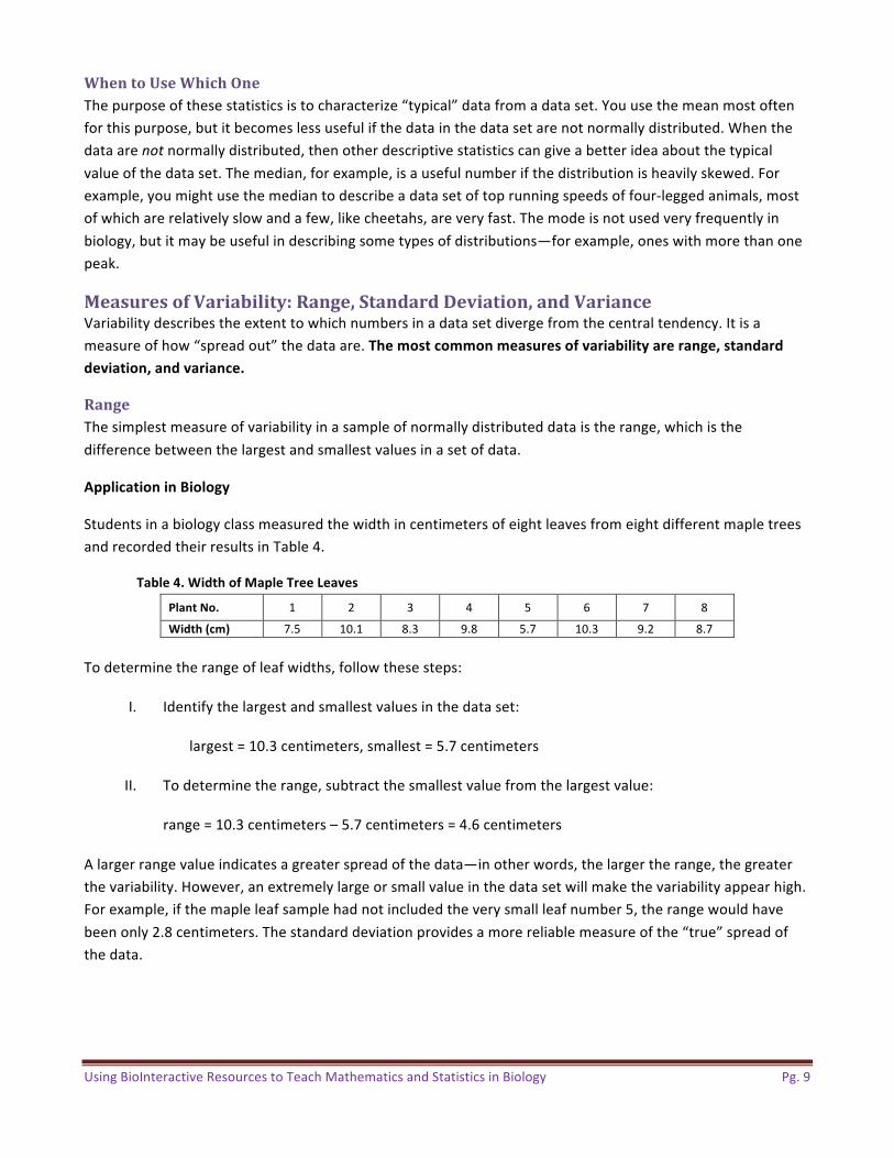
StudentsinabiologyclassmeasuredthewidthincentimetersofeightleavesfromeightdifferentmapletreesandrecordedtheirresultsinTable4.

Table4.WidthofMapleTreeLeaves

PlantNo. 1 2 3 4 5 6 7 8

Width(cm) 7.5 10.1 8.3 9.8 5.7 10.3 9.2 8.7Todeterminetherangeofleafwidths,followthesesteps:

I. Identifythelargestandsmallestvaluesinthedataset:

largest=10.3centimeters,smallest=5.7centimeters

II. Todeterminetherange,subtractthesmallestvaluefromthelargestvalue:

range=10.3centimeters–5.7centimeters=4.6centimeters

Alargerrangevalueindicatesagreaterspreadofthedata—inotherwords,thelargertherange,thegreaterthevariability.However,anextremelylargeorsmallvalueinthedatasetwillmakethevariabilityappearhigh.Forexample,ifthemapleleafsamplehadnotincludedtheverysmallleafnumber5,therangewouldhavebeenonly2.8centimeters.Thestandarddeviationprovidesamorereliablemeasureofthe“true”spreadofthedata.


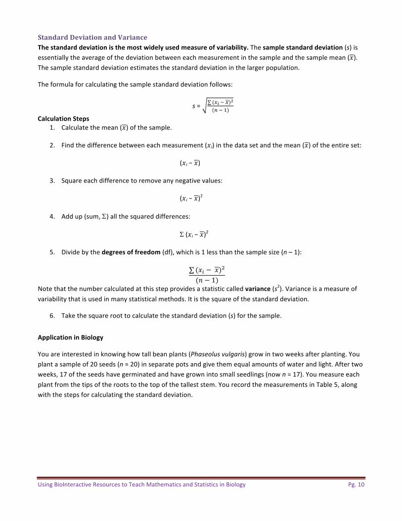
StandardDeviationandVarianceThestandarddeviationisthemostwidelyusedmeasureofvariability.Thesamplestandarddeviation(s)isessentiallytheaverageofthedeviationbetweeneachmeasurementinthesampleandthesamplemean(&).Thesamplestandarddeviationestimatesthestandarddeviationinthelargerpopulation.

Theformulaforcalculatingthesamplestandarddeviationfollows:

s= ∑ (*+0*)1(,02)

CalculationSteps1. Calculatethemean(&)ofthesample.

2. Findthedifferencebetweeneachmeasurement(&i)inthedatasetandthemean(&)oftheentireset:

(&i−&)3. Squareeachdifferencetoremoveanynegativevalues:

(&i−&)24. Addup(sum,S)allthesquareddifferences:

S (&i−&)25. Dividebythedegreesoffreedom(df),whichis1lessthanthesamplesize(n–1):

∑ (&' − &).(# − 1)

Notethatthenumbercalculatedatthisstepprovidesastatisticcalledvariance(s2).Varianceisameasureofvariabilitythatisusedinmanystatisticalmethods.Itisthesquareofthestandarddeviation.

6. Takethesquareroottocalculatethestandarddeviation(s)forthesample.


Youareinterestedinknowinghowtallbeanplants(Phaseolusvulgaris)growintwoweeksafterplanting.Youplantasampleof20seeds(n=20)inseparatepotsandgivethemequalamountsofwaterandlight.Aftertwoweeks,17oftheseedshavegerminatedandhavegrownintosmallseedlings(nown=17).Youmeasureeachplantfromthetipsoftherootstothetopofthetalleststem.YourecordthemeasurementsinTable5,alongwiththestepsforcalculatingthestandarddeviation.


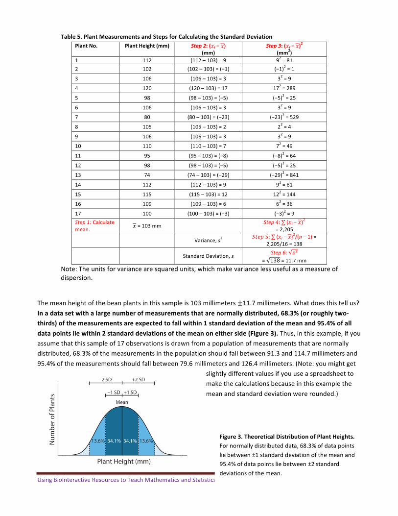
Table5.PlantMeasurementsandStepsforCalculatingtheStandardDeviation

PlantNo. PlantHeight(mm) Step2:(&i−&)(mm)

Step3:(&i−&)2(mm

2)

1 112 (112–103)=9 92=812 102 (102–103)=(−1) (−1)2=1

3 106 (106–103)=3 32=9

4 120 (120–103)=17 172=289

5 98 (98–103)=(−5) (−5)2=25

6 106 (106–103)=3 32=9

7 80 (80–103)=(−23) (−23)2=529

8 105 (105–103)=2 22=4

9 106 (106–103)=3 32=9

10 110 (110–103)=7 72=49

11 95 (95–103)=(−8) (−8)2=64

12 98 (98–103)=(−5) (−5)2=25

13 74 (74–103)=(−29) (−29)2=841

14 112 (112–103)=9 92=81

15 115 (115–103)=12 122=144

16 109 (109–103)=6 62=36

17 100 (100–103)=(−3) (−3)2=9Step1:Calculatemean. &=103mm Step4:∑ (&i−&)2

=2,205

Variance,s2 KLMN5:∑ (&i−&)2/(n–1)=2,205/16=138

StandardDeviation,s Step6: -.= 138=11.7mm

Note:Theunitsforvariancearesquaredunits,whichmakevariancelessusefulasameasureofdispersion.

Themeanheightofthebeanplantsinthissampleis103millimeters±11.7millimeters.Whatdoesthistellus?Inadatasetwithalargenumberofmeasurementsthatarenormallydistributed,68.3%(orroughlytwo-

thirds)ofthemeasurementsareexpectedtofallwithin1standarddeviationofthemeanand95.4%ofall

datapointsliewithin2standarddeviationsofthemeanoneitherside(Figure3).Thus,inthisexample,ifyouassumethatthissampleof17observationsisdrawnfromapopulationofmeasurementsthatarenormallydistributed,68.3%ofthemeasurementsinthepopulationshouldfallbetween91.3and114.7millimetersand95.4%ofthemeasurementsshouldfallbetween79.6millimetersand126.4millimeters.(Note:youmightget

slightlydifferentvaluesifyouuseaspreadsheettomakethecalculationsbecauseinthisexamplethemeanandstandarddeviationwererounded.)

Figure3.TheoreticalDistributionofPlantHeights.

Fornormallydistributeddata,68.3%ofdatapointsliebetween±1standarddeviationofthemeanand95.4%ofdatapointsliebetween±2standarddeviationsofthemean.

Num

ber o

f Pla

nts

Plant Height (mm)

34.1%13.6% 34.1% 13.6%

Mean

–2 SD +2 SD

–1 SD +1 SD


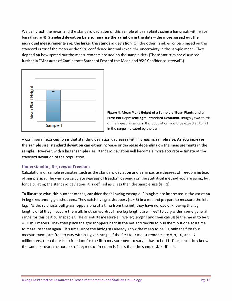
Wecangraphthemeanandthestandarddeviationofthissampleofbeanplantsusingabargraphwitherrorbars(Figure4).Standarddeviationbarssummarizethevariationinthedata—themorespreadoutthe

individualmeasurementsare,thelargerthestandarddeviation.Ontheotherhand,errorbarsbasedonthestandarderrorofthemeanorthe95%confidenceintervalrevealtheuncertaintyinthesamplemean.Theydependonhowspreadoutthemeasurementsareandonthesamplesize.(Thesestatisticsarediscussedfurtherin“MeasuresofConfidence:StandardErroroftheMeanand95%ConfidenceInterval”.)

Figure4.MeanPlantHeightofaSampleofBeanPlantsandan

ErrorBarRepresenting±1StandardDeviation.Roughlytwo-thirdsofthemeasurementsinthispopulationwouldbeexpectedtofallintherangeindicatedbythebar.

Acommonmisconceptionisthatstandarddeviationdecreaseswithincreasingsamplesize.Asyouincreasethesamplesize,standarddeviationcaneitherincreaseordecreasedependingonthemeasurementsinthe

sample.However,withalargersamplesize,standarddeviationwillbecomeamoreaccurateestimateofthestandarddeviationofthepopulation.

UnderstandingDegreesofFreedomCalculationsofsampleestimates,suchasthestandarddeviationandvariance,usedegreesoffreedominsteadofsamplesize.Thewayyoucalculatedegreesoffreedomdependsonthestatisticalmethodyouareusing,butforcalculatingthestandarddeviation,itisdefinedas1lessthanthesamplesize(n−1).

Toillustratewhatthisnumbermeans,considerthefollowingexample.Biologistsareinterestedinthevariationinlegsizesamonggrasshoppers.Theycatchfivegrasshoppers(#=5)inanetandpreparetomeasuretheleftlegs.Asthescientistspullgrasshoppersoneatatimefromthenet,theyhavenowayofknowingtheleglengthsuntiltheymeasurethemall.Inotherwords,allfiveleglengthsare“free”tovarywithinsomegeneralrangeforthisparticularspecies.Thescientistsmeasureallfiveleglengthsandthencalculatethemeantobex=10millimeters.Theythenplacethegrasshoppersbackinthenetanddecidetopullthemoutoneatatimetomeasurethemagain.Thistime,sincethebiologistsalreadyknowthemeantobe10,onlythefirstfourmeasurementsarefreetovarywithinagivenrange.Ifthefirstfourmeasurementsare8,9,10,and12millimeters,thenthereisnofreedomforthefifthmeasurementtovary;ithastobe11.Thus,oncetheyknowthesamplemean,thenumberofdegreesoffreedomis1lessthanthesamplesize,df = 4.


MeasuresofConfidence:StandardErroroftheMeanand95%ConfidenceIntervalThestandarddeviationprovidesameasureofthespreadofthedatafromthemean.Adifferenttypeofstatisticrevealstheuncertaintyinthecalculationofthemean.

Thesamplemeanisnotnecessarilyidenticaltothemeanoftheentirepopulation.Infact,everytimeyoutakeasampleandcalculateasamplemean,youwouldexpectaslightlydifferentvalue.Inotherwords,thesamplemeansthemselveshavevariability.Thisvariabilitycanbeexpressedbycalculatingthestandarderrorofthemean(abbreviatedasSE*orSEM).

Toillustratethispoint,assumethatthereisapopulationofaspeciesofanolelizardslivingonanislandoftheCaribbean.Ifyouwereabletomeasurethelengthofthehindlimbsofeveryindividualinthispopulationandthencalculatethemean,youwouldknowthevalueofthepopulationmean.However,therearethousandsofindividuals,soyoutakeasampleof10anolesandcalculatethemeanhindlimblengthforthatsample.Anotherresearcherworkingonthatislandmightcatchanothersampleof10anolesandcalculatethemeanhindlimblengthforthissample,andsoon.Thesamplemeansofmanydifferentsampleswouldbenormallydistributed.Thestandarderrorofthemeanrepresentsthestandarddeviationofsuchadistributionandestimateshowclosethesamplemeanistothepopulationmean.

Thegreatereachsamplesize(i.e.,50ratherthan10anoles),themorecloselythesamplemeanwillestimatethepopulationmean,andthereforethestandarderrorofthemeanbecomessmaller.

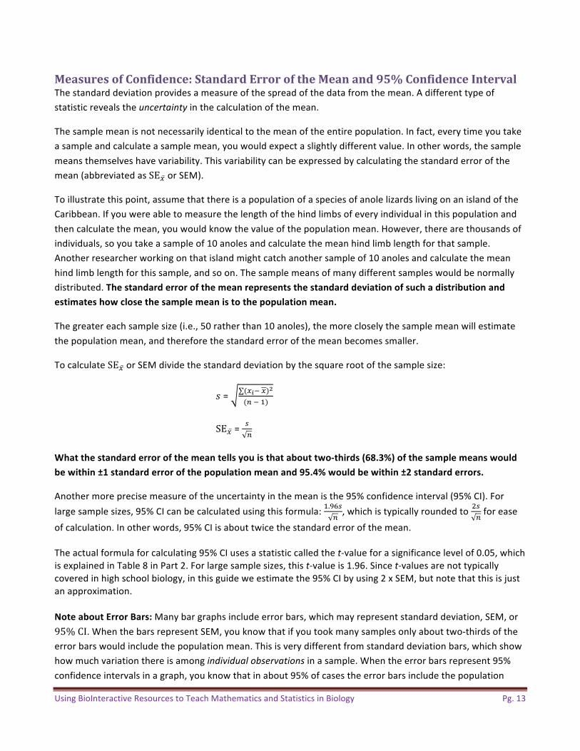
TocalculateSE*orSEMdividethestandarddeviationbythesquarerootofthesamplesize:

-= ∑(*+0*)1(,02)

SE*= 5,

Whatthestandarderrorofthemeantellsyouisthatabouttwo-thirds(68.3%)ofthesamplemeanswould

bewithin±1standarderrorofthepopulationmeanand95.4%wouldbewithin±2standarderrors.

Anothermoreprecisemeasureoftheuncertaintyinthemeanisthe95%confidenceinterval(95%CI).Forlargesamplesizes,95%CIcanbecalculatedusingthisformula:2.785, ,whichistypicallyroundedto.5,foreaseofcalculation.Inotherwords,95%CIisabouttwicethestandarderrorofthemean.Theactualformulaforcalculating95%CIusesastatisticcalledthet-valueforasignificancelevelof0.05,whichisexplainedinTable8inPart2.Forlargesamplesizes,thist-valueis1.96.Sincet-valuesarenottypicallycoveredinhighschoolbiology,inthisguideweestimatethe95%CIbyusing2xSEM,butnotethatthisisjustanapproximation.NoteaboutErrorBars:Manybargraphsincludeerrorbars,whichmayrepresentstandarddeviation,SEM,or95%CI.WhenthebarsrepresentSEM,youknowthatifyoutookmanysamplesonlyabouttwo-thirdsoftheerrorbarswouldincludethepopulationmean.Thisisverydifferentfromstandarddeviationbars,whichshowhowmuchvariationthereisamongindividualobservationsinasample.Whentheerrorbarsrepresent95%confidenceintervalsinagraph,youknowthatinabout95%ofcasestheerrorbarsincludethepopulation


mean.IfagraphshowserrorbarsthatrepresentSEM,youcanestimatethe95%confidenceintervalbymakingthebarstwiceasbig—thisisafairlyaccurateapproximationforlargesamplesizes,butforsmallsamplesthe95%confidenceintervalsareactuallymorethantwiceasbigastheSEMs.

ApplicationinBiology—Example1

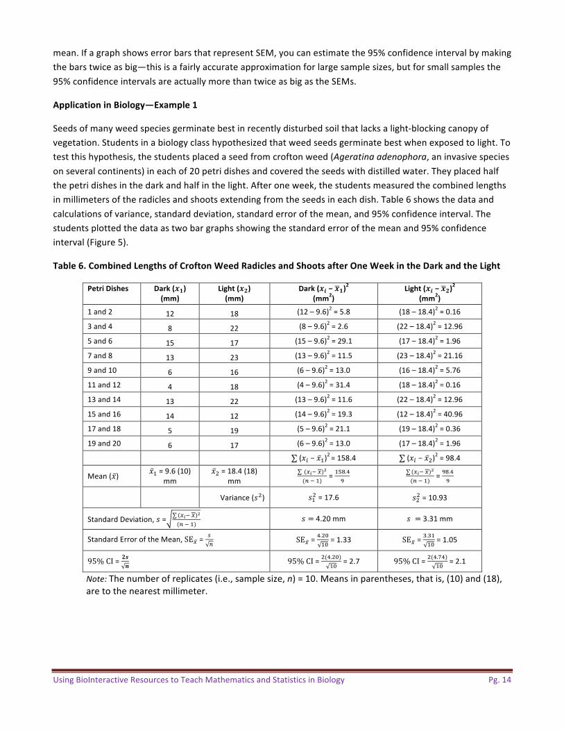
Seedsofmanyweedspeciesgerminatebestinrecentlydisturbedsoilthatlacksalight-blockingcanopyofvegetation.Studentsinabiologyclasshypothesizedthatweedseedsgerminatebestwhenexposedtolight.Totestthishypothesis,thestudentsplacedaseedfromcroftonweed(Ageratinaadenophora,aninvasivespeciesonseveralcontinents)ineachof20petridishesandcoveredtheseedswithdistilledwater.Theyplacedhalfthepetridishesinthedarkandhalfinthelight.Afteroneweek,thestudentsmeasuredthecombinedlengthsinmillimetersoftheradiclesandshootsextendingfromtheseedsineachdish.Table6showsthedataandcalculationsofvariance,standarddeviation,standarderrorofthemean,and95%confidenceinterval.Thestudentsplottedthedataastwobargraphsshowingthestandarderrorofthemeanand95%confidenceinterval(Figure5).

Table6.CombinedLengthsofCroftonWeedRadiclesandShootsafterOneWeekintheDarkandtheLight

PetriDishes Dark(Z[)(mm)

Light(Z\)(mm)

Dark(Z]−Z[)2(mm

2)

Light(Z]−Z\)2(mm

2)

1and2 12 18 (12–9.6)2=5.8 (18–18.4)2=0.16

3and4 8 22 (8–9.6)2=2.6 (22–18.4)2=12.96

5and6 15 17 (15–9.6)2=29.1 (17–18.4)2=1.96

7and8 13 23 (13–9.6)2=11.5 (23–18.4)2=21.16

9and10 6 16 (6–9.6)2=13.0 (16–18.4)2=5.76

11and12 4 18 (4–9.6)2=31.4 (18–18.4)2=0.16

13and14 13 22 (13–9.6)2=11.6 (22–18.4)2=12.96

15and16 14 12 (14–9.6)2=19.3 (12–18.4)2=40.96

17and18 5 19 (5–9.6)2=21.1 (19–18.4)2=0.36

19and20 6 17 (6–9.6)2=13.0 (17–18.4)2=1.96

∑(&'−&2)2=158.4 ∑(&'−&.)2=98.4

Mean(&) &2=9.6(10)mm

&.=18.4(18)mm

(*+0*)1(,02) =2^_.`7 ∑ (*+0*)1

(,02) =7_.`7

Variance(-.) -2.=17.6 -..=10.93

StandardDeviation,-= ∑ (*+0*)1(,02) - =4.20mm - =3.31mm

StandardErroroftheMean,SE*= 5, SE*=`..a2a=1.33 SE*=b.b22a=1.05

95%CI=\cd 95%CI=.(`..a)2a =2.7 95%CI=.(`.e`)2a =2.1

Note:Thenumberofreplicates(i.e.,samplesize,n)=10.Meansinparentheses,thatis,(10)and(18),aretothenearestmillimeter.


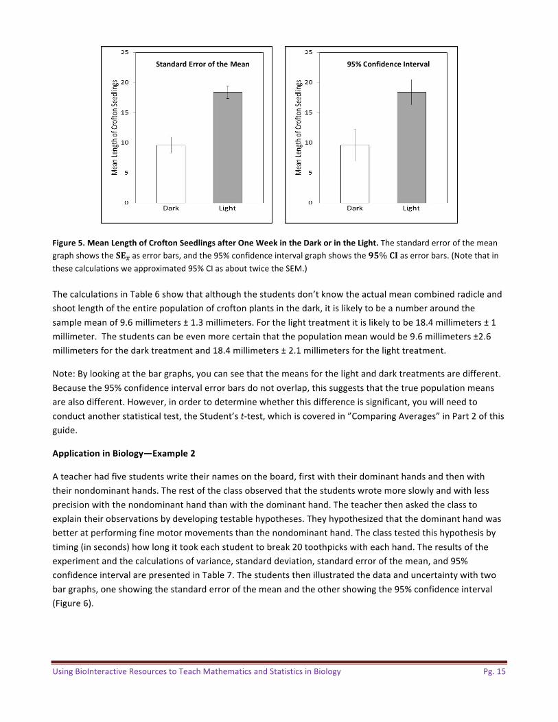
Figure5.MeanLengthofCroftonSeedlingsafterOneWeekintheDarkorintheLight.ThestandarderrorofthemeangraphshowsthefgZaserrorbars,andthe95%confidenceintervalgraphshowsthehi%jkaserrorbars.(Notethatinthesecalculationsweapproximated95%CIasabouttwicetheSEM.)ThecalculationsinTable6showthatalthoughthestudentsdon’tknowtheactualmeancombinedradicleandshootlengthoftheentirepopulationofcroftonplantsinthedark,itislikelytobeanumberaroundthesamplemeanof9.6millimeters±1.3millimeters.Forthelighttreatmentitislikelytobe18.4millimeters±1millimeter.Thestudentscanbeevenmorecertainthatthepopulationmeanwouldbe9.6millimeters±2.6millimetersforthedarktreatmentand18.4millimeters±2.1millimetersforthelighttreatment.

Note:Bylookingatthebargraphs,youcanseethatthemeansforthelightanddarktreatmentsaredifferent.Becausethe95%confidenceintervalerrorbarsdonotoverlap,thissuggeststhatthetruepopulationmeansarealsodifferent.However,inordertodeterminewhetherthisdifferenceissignificant,youwillneedtoconductanotherstatisticaltest,theStudent’st-test,whichiscoveredin”ComparingAverages”inPart2ofthisguide.


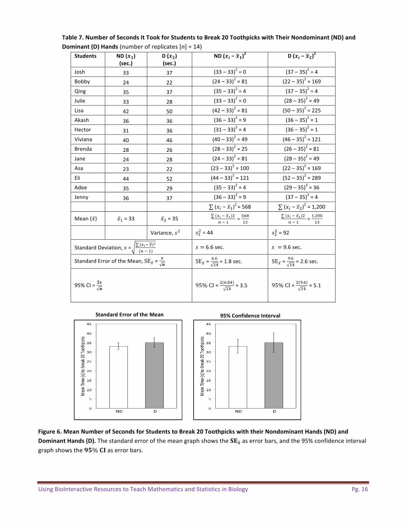
Ateacherhadfivestudentswritetheirnamesontheboard,firstwiththeirdominanthandsandthenwiththeirnondominanthands.Therestoftheclassobservedthatthestudentswrotemoreslowlyandwithlessprecisionwiththenondominanthandthanwiththedominanthand.Theteacherthenaskedtheclasstoexplaintheirobservationsbydevelopingtestablehypotheses.Theyhypothesizedthatthedominanthandwasbetteratperformingfinemotormovementsthanthenondominanthand.Theclasstestedthishypothesisbytiming(inseconds)howlongittookeachstudenttobreak20toothpickswitheachhand.Theresultsoftheexperimentandthecalculationsofvariance,standarddeviation,standarderrorofthemean,and95%confidenceintervalarepresentedinTable7.Thestudentsthenillustratedthedataanduncertaintywithtwobargraphs,oneshowingthestandarderrorofthemeanandtheothershowingthe95%confidenceinterval(Figure6).

StandardErroroftheMean 95%ConfidenceInterval


Table7.NumberofSecondsItTookforStudentstoBreak20ToothpickswithTheirNondominant(ND)and

Dominant(D)Hands(numberofreplicates[n]=14)Students ND(Z[)

(sec.)

D(Z\)(sec.)

ND(Z]−Z[)2 D(Z]−Z\)2

Josh 33 37 (33–33)2=0 (37–35)2=4

Bobby 24 22 (24–33)2=81 (22–35)2=169

Qing 35 37 (35–33)2=4 (37–35)2=4

Julie 33 28 (33–33)2=0 (28–35)2=49

Lisa 42 50 (42–33)2=81 (50–35)2=225

Akash 36 36 (36–33)2=9 (36–35)2=1

Hector 31 36 (31–33)2=4 (36–35)2=1

Viviana 40 46 (40–33)2=49 (46–35)2=121

Brenda 28 26 (28–33)2=25 (26–35)2=81

Jane 24 28 (24–33)2=81 (28–35)2=49

Asa 23 22 (23–33)2=100 (22–35)2=169

Eli 44 52 (44–33)2=121 (52–35)2=289

Adee 35 29 (35–33)2=4 (29–35)2=36

Jenny 36 37 (36–33)2=9 (37–35)2=4

∑(&'−&2)2=568 ∑(&'−&.)2=1,200Mean(&) &2=33 &.=35 ∑(*+0*:).

,02 =^8_2b ∑(*+0*1).

,02 =2,.aa2b

Variance,-. -2.=44 -..=92

StandardDeviation,-= ∑ (*+0*)1(,02) - =6.6sec. - =9.6sec.

StandardErroroftheMean,SE*= cd SE*= 8.82`=1.8sec. SE*= 7.82`=2.6sec.

95%CI=\cd 95%CI=.(8._`)2` =3.5 95%CI=.(7.8)2` =5.1

Figure6.MeanNumberofSecondsforStudentstoBreak20ToothpickswiththeirNondominantHands(ND)and

DominantHands(D).ThestandarderrorofthemeangraphshowsthefgZaserrorbars,andthe95%confidenceintervalgraphshowsthehi%jkaserrorbars.

StandardErroroftheMean 95%ConfidenceInterval


Thecalculationsindicatethatittakesabout31.2seconds(33−1.8)to34.8seconds(33+1.8)forthenondominanthandtobreaktoothpicksandabout32.4to37.6secondsforthedominanthand.Youcanbemorecertainthattheaverageforthenondominanthandwouldfallsomewherebetween29.5seconds(33–3.5)and36.5seconds(33+3.5)andforthedominanthandsfallssomewherebetween29.9seconds(35–5.1)and40.1seconds(35+5.1).

Thisendsthepartondescriptivestatistics.GoingbacktothefinchdatasetinTable1andFigure1ofPart1,

howwouldyoucalculatethesamplemeansforbeaksizesofthesurvivorsandnonsurvivors?Istheremore

variabilityamongsurvivorsornonsurvivors?Whatistheuncertaintyinyoursamplemeanestimates?To

findtheanswerstothesequestions,seethe“EvolutioninAction:DataAnalysis”activitiesat

http://www.hhmi.org/biointeractive/evolution-action-data-analysis.

Part2:InferentialStatisticsUsedinBiologyInferentialstatisticstestsstatisticalhypotheses,whicharedifferentfromexperimentalhypotheses.Tounderstandwhatthismeans,assumethatyoudoanexperimenttotestwhether“nitrogenpromotesplantgrowth.”Thisisanexperimentalhypothesisbecauseittellsyousomethingaboutthebiologyofplantgrowth.Totestthishypothesis,yougrow10beanplantsindirtwithaddednitrogenand10beanplantsindirtwithoutaddednitrogen.Youfindoutthatthemeansofthesetwosamplesare13.2centimetersand11.9centimeters,respectively.Doesthisresultindicatethatthereisadifferencebetweenthetwopopulationsandthatnitrogenmightpromoteplantgrowth?Oristhedifferenceinthetwomeansmerelyduetochance?Astatisticaltestisrequiredtodiscriminatebetweenthesepossibilities.

Statisticaltestsevaluatestatisticalhypotheses.Thestatisticalnullhypothesis(symbolizedbyH0andpronouncedH-naught)isastatementthatyouwanttotest.Inthiscase,ifyougrow10plantswithnitrogenand10without,thenullhypothesisisthatthereisnodifferenceinthemeanheightsofthetwogroupsandanyobserveddifferencebetweenthetwogroupswouldhaveoccurredpurelybychance.ThealternativehypothesistoH0issymbolizedbyH1andusuallysimplystatesthatthereisadifferencebetweenthepopulations.

Thestatisticalnullandalternativehypothesesarestatementsaboutthedatathatshouldfollowfromthe

experimentalhypothesis.

SignificanceTesting:Thea(Alpha)LevelBeforeyouperformastatisticaltestontheplantgrowthdata,youshoulddetermineanacceptablesignificancelevelofthenullstatisticalhypothesis.Thatis,ask,whendoIthinkmyresultsandthusmyteststatisticaresounusualthatInolongerthinkthedifferencesobservedinmydataaresimplyduetochance?Thissignificancelevelisalsoknownas“alpha”andissymbolizedbya.

Thesignificancelevelistheprobabilityofgettingateststatisticrareenoughthatyouarecomfortable

rejectingthenullhypothesis(H0).(Seethe“Probability”sectionofPart3forfurtherdiscussionofprobability.)Thewidelyacceptedsignificancelevelinbiologyis0.05.Iftheprobability(p)valueislessthan0.05,yourejectthenullhypothesis;ifpisgreaterthanorequalto0.05,youdon’trejectthenullhypothesis.


ComparingAverages:TheStudent’st-TestforIndependentSamplesTheStudent’st-testisusedtocomparethemeansoftwosamplestodeterminewhethertheyare

statisticallydifferent.Forexample,youcalculatedthesamplemeansofsurvivorandnonsurvivorfinchesfromTable1andyougotdifferentnumbers.Whatistheprobabilityofgettingthisdifferenceinmeans,ifthepopulationmeansarereallythesame?

Thet-testassessestheprobabilityofgettingaresultmoredifferentthantheobservedresult(i.e.,thevaluesyoucalculatedforthemeansshowninFigure1)ifthenullstatisticalhypothesis(H0)istrue.Typically,thenullstatisticalhypothesisinat-testisthatthemeanofthepopulationfromwhichsample1came(i.e.,themeanbeaksizeofsurvivors)isequaltothemeanofthepopulationfromwhichsample2came(i.e.,themeanbeaksizeofthenonsurvivors),orm1=m2.RejectingH0supportsthealternativehypothesis,H1,thatthemeansaresignificantlydifferent(m1¹m2).Inthefinchexample,thet-testdetermineswhetheranyobserveddifferencesbetweenthemeansofthetwogroupsoffinches(9.67millimetersversus9.11millimeters)arestatisticallysignificantorhavelikelyoccurredsimplybychance.

At-testcalculatesasinglestatistic,t,ortobs,whichiscomparedtoacriticalt-statistic(tcrit):

tobs=|*:0*1|no

Tocalculatethestandarderror(SE)specificforthet-test,wecalculatethesamplemeansandthevariance(s2)forthetwosamplesbeingcompared—thesamplesize(n)foreachsamplemustbeknown:

SE= 5:1,:+ 51

1

,1

Thus,thecompleteequationforthet-testis

tobs=|*:0*1|

;:1<:=;1

1<1

CalculationSteps

1. Calculatethemeanofeachsamplepopulationandsubtractonefromtheother.Taketheabsolutevalueofthisdifference.

2. Calculatethestandarderror,SE.Tocomputeit,calculatethevarianceofeachsample(s2),anddivideit

bythenumberofmeasuredvaluesinthatsample(n,thesamplesize).Addthesetwovaluesandthentakethesquareroot.

3. Dividethedifferencebetweenthemeansbythestandarderrortogetavaluefort.Comparethe

calculatedvaluetotheappropriatecriticalt-valueinTable8.Table8showstcritfordifferentdegreesoffreedomforasignificancevalueof0.05.Thedegreesoffreedomiscalculatedbyaddingthenumber

ofdatapointsinthetwogroupscombined,minus2.Notethatyoudonothavetohavethesamenumberofdatapointsineachgroup.

4. Ifthecalculatedt-valueisgreaterthantheappropriatecriticalt-value,thisindicatesthatyouhave

enoughevidencetosupportthehypothesisthatthemeansofthetwosamplesaresignificantlydifferentattheprobabilityvaluelisted(inthiscase,0.05).Ifthecalculatedtissmaller,thenyoucannotrejectthenullhypothesisthatthereisnosignificantdifference.


Table8.Criticalt-ValuesforaSignificanceLevela=0.05DegreesofFreedom(df) tcrit(a=0.05)1 12.712 4.303 3.184 2.785 2.576 2.457 2.368 2.319 2.2610 2.2311 2.2012 2.1813 2.1614 2.1415 2.1316 2.1217 2.1118 2.1019 2.0920 2.0921 2.0822 2.0723 2.0724 2.0625 2.0626 2.0627 2.0528 2.0529 2.0430 2.0440 2.0260 2.00120 1.98Infinity 1.96

Note:Therearetwobasicversionsofthet-test.Theversionpresentedhereassumesthateachsamplewastakenfromadifferentpopulation,andsothesamplesarethereforeindependentofoneanother.Forexample,thesurvivorandnonsurvivorfinchesaredifferentindividuals,independentofoneanother,andthereforeconsideredunpaired.Ifwewerecomparingthelengthsofrightandleftwingsonallthefinches,thesampleswouldbeclassifiedaspaired.Pairedsamplesrequireadifferentversionofthet-testknownasapairedt-test,aversiontowhichmanystatisticalprogramsdefault.Thepairedt-testisnotdiscussedinthisguide.


Afterasmallpopulationofcrayfishwasaccidentallyreleasedintoashallowpond,biologistsnoticedthatthecrayfishhadconsumednearlyalloftheunderwaterplantpopulation;aquaticinvertebrates,suchasthewaterflea(Daphniasp.),hadalsodeclined.ThebiologistsknewthatthemainpredatorofDaphniaisthegoldfish,andtheyhypothesizedthattheunderwaterplantsprotectedtheDaphniafromthegoldfishbyprovidinghidingplaces.TheDaphnialosttheirprotectionastheunderwaterplantsdisappeared.Thebiologistsdesignedan


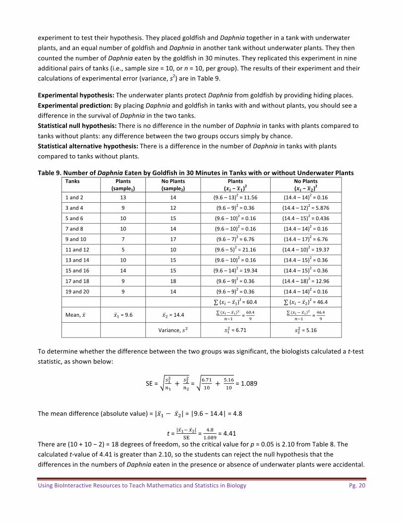
experimenttotesttheirhypothesis.TheyplacedgoldfishandDaphniatogetherinatankwithunderwaterplants,andanequalnumberofgoldfishandDaphniainanothertankwithoutunderwaterplants.TheythencountedthenumberofDaphniaeatenbythegoldfishin30minutes.Theyreplicatedthisexperimentinnineadditionalpairsoftanks(i.e.,samplesize=10,orn=10,pergroup).Theresultsoftheirexperimentandtheircalculationsofexperimentalerror(variance,s2)areinTable9.

Experimentalhypothesis:TheunderwaterplantsprotectDaphniafromgoldfishbyprovidinghidingplaces.Experimentalprediction:ByplacingDaphniaandgoldfishintankswithandwithoutplants,youshouldseeadifferenceinthesurvivalofDaphniainthetwotanks.Statisticalnullhypothesis:ThereisnodifferenceinthenumberofDaphniaintankswithplantscomparedtotankswithoutplants:anydifferencebetweenthetwogroupsoccurssimplybychance.Statisticalalternativehypothesis:ThereisadifferenceinthenumberofDaphniaintankswithplantscomparedtotankswithoutplants.

Table9.NumberofDaphniaEatenbyGoldfishin30MinutesinTankswithorwithoutUnderwaterPlants

Tanks Plants

(sample1)

NoPlants

(sample2)

Plants

(Z]−Z[)2NoPlants

(Z]−Z\)21and2 13 14 (9.6–13)2=11.56 (14.4–14)2=0.16

3and4 9 12 (9.6–9)2=0.36 (14.4–12)2=5.876

5and6 10 15 (9.6–10)2=0.16 (14.4–15)2=0.436

7and8 10 14 (9.6–10)2=0.16 (14.4–14)2=0.16

9and10 7 17 (9.6–7)2=6.76 (14.4–17)2=6.76

11and12 5 10 (9.6–5)2=21.16 (14.4–10)2=19.37

13and14 10 15 (9.6–10)2=0.16 (14.4–15)2=0.36

15and16 14 15 (9.6–14)2=19.34 (14.4–15)2=0.36

17and18 9 18 (9.6–9)2=0.36 (14.4–18)2=12.96

19and20 9 14 (9.6–9)2=0.36 (14.4–14)2=0.16

∑(&'−&2)2=60.4 ∑(&'−&.)2=46.4

Mean,& &2=9.6 &.=14.4 ∑(*+0*:)1,02 =8a.`7 ∑(*+0*:)1

,02 =`8.`7

Variance,-. -2.=6.71 -..=5.16

Todeterminewhetherthedifferencebetweenthetwogroupswassignificant,thebiologistscalculatedat-teststatistic,asshownbelow:

SE= 5:1,:+ 51

1

,1= 8.e2

2a + ^.282a =1.089

Themeandifference(absolutevalue)=|&2 − &.|=|9.6−14.4|=4.8

t=|*:0*1|qr = `._2.a_7=4.41Thereare(10+10−2)=18degreesoffreedom,sothecriticalvalueforp=0.05is2.10fromTable8.Thecalculatedt-valueof4.41isgreaterthan2.10,sothestudentscanrejectthenullhypothesisthatthedifferencesinthenumbersofDaphniaeateninthepresenceorabsenceofunderwaterplantswereaccidental.


Sowhatcantheyconclude?ItispossiblethatthegoldfishatesignificantlymoreDaphniaintheabsenceofunderwaterplantsthaninthepresenceoftheplants.

AnalyzingFrequencies:TheChi-SquareTestThet-testisusedtocomparethesamplemeansoftwosetsofdata.Thechi-squaretestisusedtodeterminehowtheobservedresultscomparetoanexpectedortheoreticalresult.

Forexample,youdecidetoflipacoin50times.Youexpectaproportionof50%headsand50%tails.Basedona50:50probability,youpredict25headsand25tails.Thesearetheexpectedvalues.Youwouldrarelygetexactly25and25,buthowfaroffcanthesenumbersbewithouttheresultsbeingsignificantlydifferentfromwhatyouexpected?Afteryouconductyourexperiment,youget21headsand29tails(theobservedvalues).Isthedifferencebetweenobservedandexpectedresultspurelyduetochance?Orcoulditbeduetosomethingelse,suchassomethingmightbewrongwiththecoin?Thechi-squaretestcanhelpyouanswerthisquestion.Thestatisticalnullhypothesisisthattheobservedcountswillbeequaltothatexpected,andthealternativehypothesisisthattheobservednumbersaredifferentfromtheexpected.

Notethatthistestmustbeusedonrawcategoricaldata.Valuesneedtobesimplecounts,notpercentagesorproportions.Thesizeofthesampleisanimportantaspectofthechi-squaretest—itismoredifficulttodetectastatisticallysignificantdifferencebetweenexperimentalandobservedresultsinasmallsamplethaninalargesample.Twocommonapplicationsofthistestinbiologyareinanalyzingtheoutcomesofageneticcrossandthedistributionoforganismsinresponsetoanenvironmentalfactorofinterest.

Tocalculatethechi-squareteststatistic(χ2),youusetheequation

s.= ?0@ 1

@

o=observedvalues e=expectedvalues

χ2=chi-squarevalue S=summation

CalculationSteps

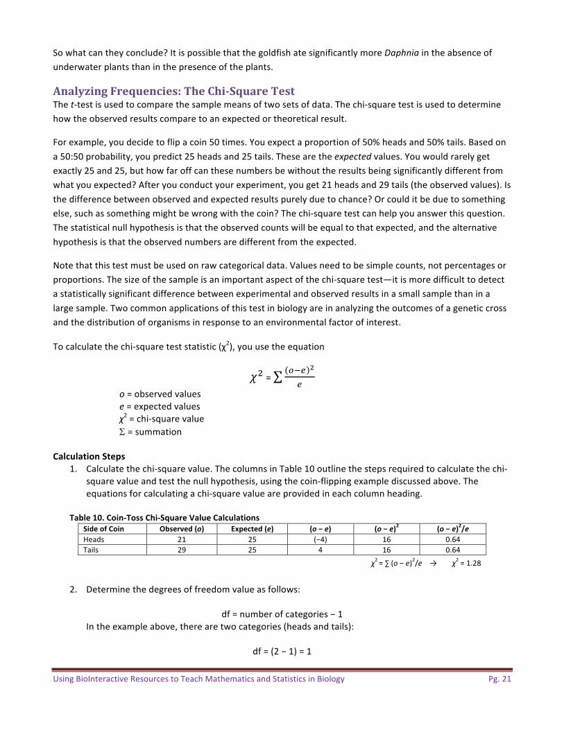
1. Calculatethechi-squarevalue.ThecolumnsinTable10outlinethestepsrequiredtocalculatethechi-squarevalueandtestthenullhypothesis,usingthecoin-flippingexamplediscussedabove.Theequationsforcalculatingachi-squarevalueareprovidedineachcolumnheading.

Table10.Coin-TossChi-SquareValueCalculations

SideofCoin Observed(o) Expected(e) (o−e) (o−e)2 (o−e)2/eHeads 21 25 (−4) 16 0.64Tails 29 25 4 16 0.64

χ2=∑ (o−e)2/e→χ2=1.28

2. Determinethedegreesoffreedomvalueasfollows:

df=numberofcategories−1

Intheexampleabove,therearetwocategories(headsandtails):

df=(2−1)=1


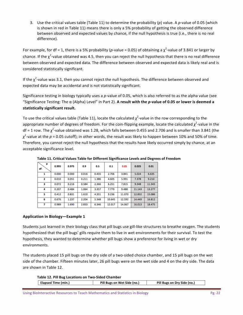
3. Usethecriticalvaluestable(Table11)todeterminetheprobability(p)value.Ap-valueof0.05(whichisshowninredinTable11)meansthereisonlya5%probabilityofgettingtheobserveddifferencebetweenobservedandexpectedvaluesbychance,ifthenullhypothesisistrue(i.e.,thereisnorealdifference).

Forexample,fordf=1,thereisa5%probability(p-value=0.05)ofobtainingaχ2-valueof3.841orlargerbychance.Iftheχ2-valueobtainedwas4.5,thenyoucanrejectthenullhypothesisthatthereisnorealdifferencebetweenobservedandexpecteddata.Thedifferencebetweenobservedandexpecteddataislikelyrealandisconsideredstatisticallysignificant.

Iftheχ2-valuewas3.1,thenyoucannotrejectthenullhypothesis.Thedifferencebetweenobservedandexpecteddatamaybeaccidentalandisnotstatisticallysignificant.

Significancetestinginbiologytypicallyusesap-valueof0.05,whichisalsoreferredtoasthealphavalue(see“SignificanceTesting:Theα(Alpha)Level”inPart2).Aresultwiththep-valueof0.05orlowerisdeemeda

statisticallysignificantresult.

Tousethecriticalvaluestable(Table11),locatethecalculatedχ2-valueintherowcorrespondingtotheappropriatenumberofdegreesoffreedom.Forthecoin-flippingexample,locatethecalculatedχ2-valueinthedf=1row.Theχ2-valueobtainedwas1.28,whichfallsbetween0.455and2.706andissmallerthan3.841(theχ2-valueatthep=0.05cutoff);inotherwords,theresultwaslikelytohappenbetween10%and50%oftime.Therefore,youcannotrejectthenullhypothesisthattheresultshavelikelyoccurredsimplybychance,atanacceptablesignificancelevel.

Table11.CriticalValuesTableforDifferentSignificanceLevelsandDegreesofFreedom


Studentsjustlearnedintheirbiologyclassthatpillbugsusegill-likestructurestobreatheoxygen.Thestudentshypothesizedthatthepillbugs’gillsrequirethemtoliveinwetenvironmentsfortheirsurvival.Totestthehypothesis,theywantedtodeterminewhetherpillbugsshowapreferenceforlivinginwetordryenvironments.

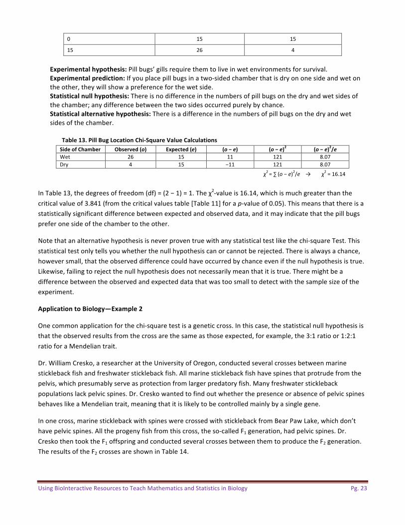
Thestudentsplaced15pillbugsonthedrysideofatwo-sidedchoicechamber,and15pillbugsonthewetsideofthechamber.Fifteenminuteslater,26pillbugswereonthewetsideand4onthedryside.ThedataareshowninTable12.

Table12.PillBugLocationsonTwo-SidedChamber

ElapsedTime(min.) PillBugsonWetSide(no.) PillBugsonDrySide(no.)


0 15 15

15 26 4

Experimentalhypothesis:Pillbugs’gillsrequirethemtoliveinwetenvironmentsforsurvival.Experimentalprediction:Ifyouplacepillbugsinatwo-sidedchamberthatisdryononesideandwetontheother,theywillshowapreferenceforthewetside.Statisticalnullhypothesis:Thereisnodifferenceinthenumbersofpillbugsonthedryandwetsidesofthechamber;anydifferencebetweenthetwosidesoccurredpurelybychance.Statisticalalternativehypothesis:Thereisadifferenceinthenumbersofpillbugsonthedryandwetsidesofthechamber.

Table13.PillBugLocationChi-SquareValueCalculations

SideofChamber Observed(o) Expected(e) (o−e) (o−e)2 (o−e)2/eWet 26 15 11 121 8.07Dry 4 15 −11 121 8.07

χ2=∑ (o−e)2/e→χ2=16.14

InTable13,thedegreesoffreedom(df)=(2−1)=1.Theχ2-valueis16.14,whichismuchgreaterthanthecriticalvalueof3.841(fromthecriticalvaluestable[Table11]forap-valueof0.05).Thismeansthatthereisastatisticallysignificantdifferencebetweenexpectedandobserveddata,anditmayindicatethatthepillbugspreferonesideofthechambertotheother.

Notethatanalternativehypothesisisneverproventruewithanystatisticaltestlikethechi-squareTest.Thisstatisticaltestonlytellsyouwhetherthenullhypothesiscanorcannotberejected.Thereisalwaysachance,howeversmall,thattheobserveddifferencecouldhaveoccurredbychanceevenifthenullhypothesisistrue.Likewise,failingtorejectthenullhypothesisdoesnotnecessarilymeanthatitistrue.Theremightbeadifferencebetweentheobservedandexpecteddatathatwastoosmalltodetectwiththesamplesizeoftheexperiment.

ApplicationtoBiology—Example2

Onecommonapplicationforthechi-squaretestisageneticcross.Inthiscase,thestatisticalnullhypothesisisthattheobservedresultsfromthecrossarethesameasthoseexpected,forexample,the3:1ratioor1:2:1ratioforaMendeliantrait.

Dr.WilliamCresko,aresearcherattheUniversityofOregon,conductedseveralcrossesbetweenmarinesticklebackfishandfreshwatersticklebackfish.Allmarinesticklebackfishhavespinesthatprotrudefromthepelvis,whichpresumablyserveasprotectionfromlargerpredatoryfish.Manyfreshwatersticklebackpopulationslackpelvicspines.Dr.CreskowantedtofindoutwhetherthepresenceorabsenceofpelvicspinesbehaveslikeaMendeliantrait,meaningthatitislikelytobecontrolledmainlybyasinglegene.

Inonecross,marinesticklebackwithspineswerecrossedwithsticklebackfromBearPawLake,whichdon’thavepelvicspines.Alltheprogenyfishfromthiscross,theso-calledF1generation,hadpelvicspines.Dr.CreskothentooktheF1offspringandconductedseveralcrossesbetweenthemtoproducetheF2generation.TheresultsoftheF2crossesareshowninTable14.


Table14.F2Generation:CrossofF1GenerationIndividuals

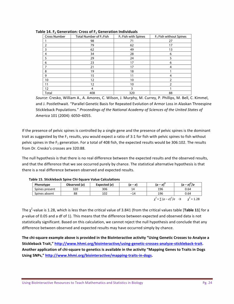
Cross Number Total Number of F2 Fish F2 Fish with Spines F2 Fish without Spines 1 98 71 27 2 79 62 17 3 62 49 13 4 34 28 6 5 29 24 5 6 23 17 6 7 21 17 4 8 19 18 1 9 15 11 4 10 12 10 2 11 12 10 2 12 4 3 1 Total 408 320 88

Source:Cresko,WilliamA.,A.Amores,C.Wilson,J.Murphy,M.Currey,P.Phillips,M.Bell,C.Kimmel,andJ.Postlethwait.“ParallelGeneticBasisforRepeatedEvolutionofArmorLossinAlaskanThreespineSticklebackPopulations.”ProceedingsoftheNationalAcademyofSciencesoftheUnitedStatesofAmerica101(2004):6050–6055.

IfthepresenceofpelvicspinesiscontrolledbyasinglegeneandthepresenceofpelvicspinesisthedominanttraitassuggestedbytheF1results,youwouldexpectaratioof3:1forfishwithpelvicspinestofishwithoutpelvicspinesintheF2generation.Foratotalof408fish,theexpectedresultswouldbe306:102.TheresultsfromDr.Cresko’scrossesare320:88.

Thenullhypothesisisthatthereisnorealdifferencebetweentheexpectedresultsandtheobservedresults,andthatthedifferencethatweseeoccurredpurelybychance.Thestatisticalalternativehypothesisisthatthereisarealdifferencebetweenobservedandexpectedresults.

Table15.SticklebackSpineChi-SquareValueCalculations

Phenotype Observed(o) Expected(e) (o−e) (o−e)2 (o−e)2/eSpinespresent 320 306 14 196 0.64Spinesabsent 88 102 −14 196 0.64

χ2=∑ (o−e)2/e→χ2=1.28

Theχ2-valueis1.28,whichislessthanthecriticalvalueof3.841(fromthecriticalvaluestable[Table11]forap-valueof0.05andadfof1).Thismeansthatthedifferencebetweenexpectedandobserveddataisnotstatisticallysignificant.Basedonthiscalculation,wecannotrejectthenullhypothesisandconcludethatanydifferencebetweenobservedandexpectedresultsmayhaveoccurredsimplybychance.

Thechi-squareexampleaboveisprovidedintheBioInteractiveactivity“UsingGeneticCrossestoAnalyzea

SticklebackTrait,”http://www.hhmi.org/biointeractive/using-genetic-crosses-analyze-stickleback-trait.

Anotherapplicationofchi-squaretogeneticsisavailableintheactivity“MappingGenestoTraitsinDogs

UsingSNPs,”http://www.hhmi.org/biointeractive/mapping-traits-in-dogs.


MeasuringCorrelationsandAnalyzingLinearRegressionCorrelationscansuggestrelationshipsbetweensetsofdata.Thecorrelationcoefficient(A)providesameasureofhowrelatedtwovariablesare,anditisexpressedasavaluebetween+1and−1.Thecloserthevalueisto0,theweakerthecorrelation.

Forexample,ifyouplotthewidthofanoak(Quercussp.)leaf(Y)onanxyscatterplotasafunctionoftheleaf’slength(X),thecorrelationcoefficient(A)indicateshowmuchwidthdependsonlength.AnA-valueequalto+1wouldindicateaperfectpositivecorrelationbetweenwidthandlength.Inotherwords,thelongeranoakleaf,thewideritis.AnA-valueof−1wouldindicateaperfectnegativecorrelation—thelongeranoakleaf,thenarroweritis.Ifthereisnocorrelationbetweentwovariables,theA-valueequals0,whichwouldmeanthatthereisnorelationshipbetweenoakleaflengthandwidth.Thenullhypothesis(H0)foracorrelationisthatthereisnocorrelationandA=0.

CalculatingAinvolvesdeterminingthesamplemeanofthepredictorvariable(&)anditsstandarddeviation(-*),thesamplemeanoftheresponsevariable(t)anditsstandarddeviation(-u),andthenumberofpairs(X,Y)ofindividualsinthesample(#):

A=B+CB;B

<+D:

E+CE;E

,02 Anotherstatistic,calledthecoefficientofdetermination,usesthesquareofA.TheA.-valuetellsusthestrengthoftherelationshipbetweenXandY.

Whencalculatingcorrelations,itisimportantforyoutorememberthatcorrelationdoesnotimplycausation.Forexample,Figure7showsthatthereisastrongnegativecorrelationbetweenthemeantemperatureofEarthoverthelast190yearsandthenumberofpiratesintheCaribbean.Clearly,adecreaseinthenumberofpiratesisnotthecauseofglobalwarming.

Figure7.MeanGlobalTemperature(°C)asaFunctionoftheApproximateNumberofPirates

intheCaribbean,1820–2000.Thelineisthelinearregression.Statisticsarecorrelationcoefficient(v)andthecoefficientofdetermination(v\).


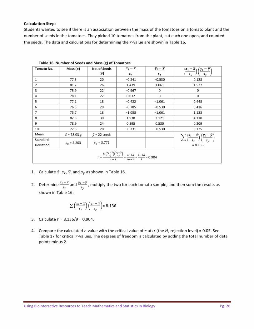
CalculationSteps

Studentswantedtoseeifthereisanassociationbetweenthemassofthetomatoesonatomatoplantandthenumberofseedsinthetomatoes.Theypicked10tomatoesfromtheplant,cuteachoneopen,andcountedtheseeds.ThedataandcalculationsfordeterminingtheA-valueareshowninTable16.

Table16.NumberofSeedsandMass(g)ofTomatoes

TomatoNo. Mass(Z) No.ofSeeds

(w)Z] − ZcZ

w] − wcw

Z] − ZcZ

w] − wcw

1 77.5 20 −0.241 −0.530 0.1282 81.2 26 1.439 1.061 1.5273 75.9 22 −0.967 0 04 78.1 22 0.032 0 05 77.1 18 −0.422 −1.061 0.4486 76.3 20 −0.785 −0.530 0.4167 75.7 18 −1.058 −1.061 1.1238 82.3 30 1.938 2.121 4.1109 78.9 24 0.395 0.530 0.20910 77.3 20 −0.331 −0.530 0.175Mean &=78.03g t=22seeds &' − &

-*t' − t-u

=8.136StandardDeviation -*=2.203 -u=3.771

A= B+CB;B

E+CE;E

,02 = _.2b82a02=_.2b87 =0.904

1. Calculate&,-*,t,and-uasshowninTable16.

2. Determine*+0*5B

andu+0u5E,multiplythetwoforeachtomatosample,andthensumtheresultsas

showninTable16:

*+0*5B

u+0u5E

=8.136

3. CalculateA=8.136/9=0.904.

4. ComparethecalculatedA-valuewiththecriticalvalueofAata(theH0rejectionlevel)=0.05.See

Table17forcriticalA-values.Thedegreesoffreedomiscalculatedbyaddingthetotalnumberofdatapointsminus2.


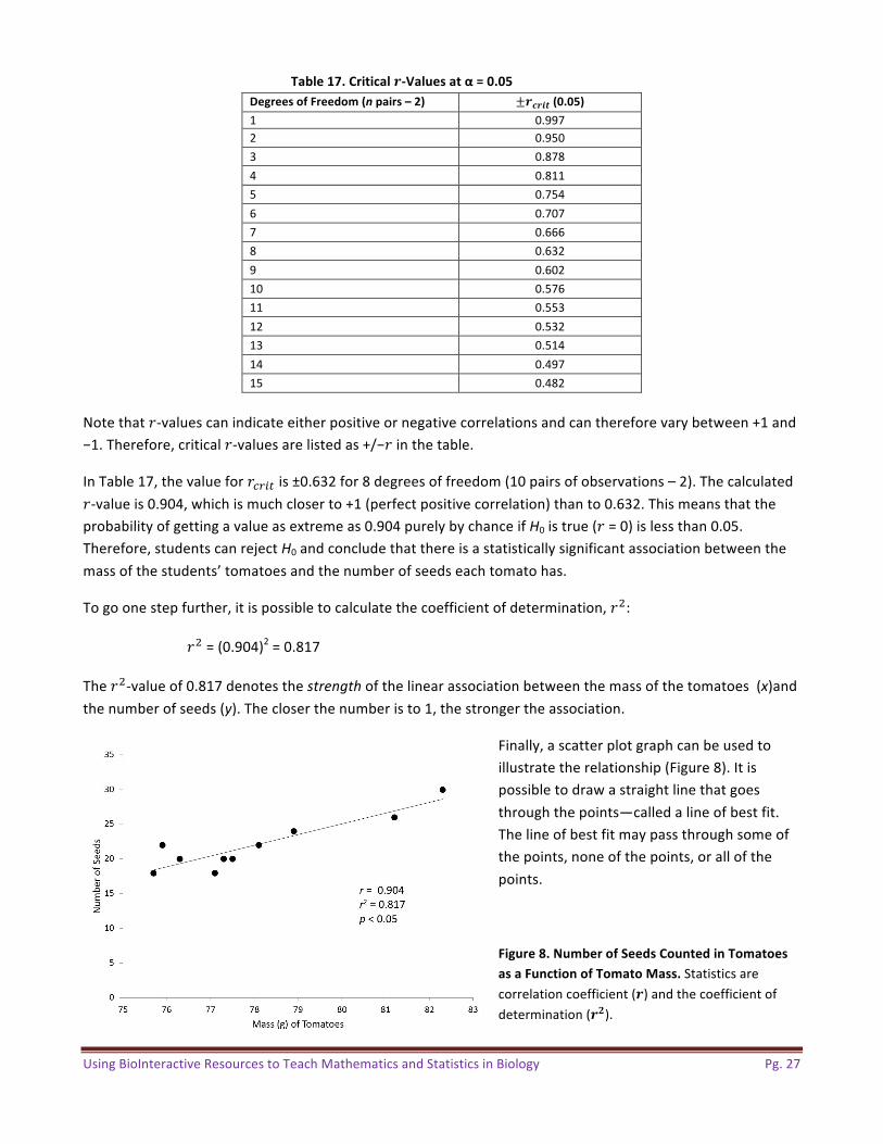
Table17.Criticalv-Valuesatα=0.05DegreesofFreedom(npairs–2) ±vxv]y(0.05)1 0.9972 0.9503 0.8784 0.8115 0.7546 0.7077 0.6668 0.6329 0.60210 0.57611 0.55312 0.53213 0.51414 0.49715 0.482

NotethatA-valuescanindicateeitherpositiveornegativecorrelationsandcanthereforevarybetween+1and−1.Therefore,criticalA-valuesarelistedas+/−Ainthetable.

InTable17,thevalueforAz{'|is±0.632for8degreesoffreedom(10pairsofobservations–2).ThecalculatedA-valueis0.904,whichismuchcloserto+1(perfectpositivecorrelation)thanto0.632.Thismeansthattheprobabilityofgettingavalueasextremeas0.904purelybychanceifH0istrue(A=0)islessthan0.05.Therefore,studentscanrejectH0andconcludethatthereisastatisticallysignificantassociationbetweenthemassofthestudents’tomatoesandthenumberofseedseachtomatohas.

Togoonestepfurther,itispossibletocalculatethecoefficientofdetermination,A.:

A.=(0.904)2=0.817TheA.-valueof0.817denotesthestrengthofthelinearassociationbetweenthemassofthetomatoes(x)andthenumberofseeds(y).Thecloserthenumberisto1,thestrongertheassociation.

Finally,ascatterplotgraphcanbeusedtoillustratetherelationship(Figure8).Itispossibletodrawastraightlinethatgoesthroughthepoints—calledalineofbestfit.Thelineofbestfitmaypassthroughsomeofthepoints,noneofthepoints,orallofthepoints.

Figure8.NumberofSeedsCountedinTomatoes

asaFunctionofTomatoMass.Statisticsarecorrelationcoefficient(v)andthecoefficientofdetermination(v\).


Thecoefficientofdeterminationisameasureofhowwelltheregressionlinerepresentsthedata.Iftheregressionlinepassesexactlythrougheverypointonthescatterplot,itwouldbeabletoexplainallofthevariation.Thefurtherthelineisawayfromthepoints,thelessitisabletoexplain.InFigure8,81.7%ofthevariationinycanbeexplainedbytherelationshipbetweenxandy.

Note:Manybiologicaltraits(i.e.,animalbehaviororphysicalappearance)varygreatlyamongindividualsinapopulation.Thus,acoefficientofdeterminationof0.817betweentwobiologicalvariablesisconsideredveryhigh.However,forastandardcurve,asdescribedin“StandardCurves”inPart3,itwouldbeconsideredlow.


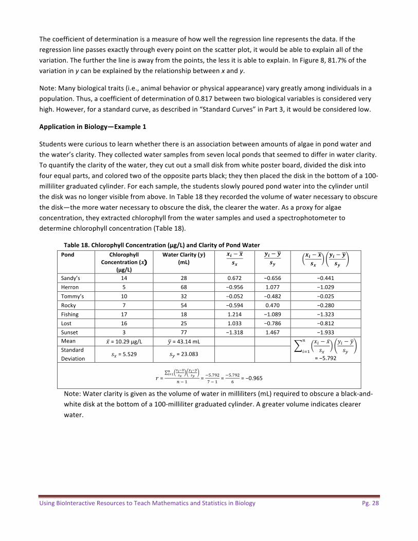
Studentswerecurioustolearnwhetherthereisanassociationbetweenamountsofalgaeinpondwaterandthewater’sclarity.Theycollectedwatersamplesfromsevenlocalpondsthatseemedtodifferinwaterclarity.Toquantifytheclarityofthewater,theycutoutasmalldiskfromwhiteposterboard,dividedthediskintofourequalparts,andcoloredtwooftheoppositepartsblack;theythenplacedthediskinthebottomofa100-millilitergraduatedcylinder.Foreachsample,thestudentsslowlypouredpondwaterintothecylinderuntilthediskwasnolongervisiblefromabove.InTable18theyrecordedthevolumeofwaternecessarytoobscurethedisk—themorewaternecessarytoobscurethedisk,theclearerthewater.Asaproxyforalgaeconcentration,theyextractedchlorophyllfromthewatersamplesandusedaspectrophotometertodeterminechlorophyllconcentration(Table18).

Table18.ChlorophyllConcentration(μg/L)andClarityofPondWater

Pond Chlorophyll

Concentration(Z)(μg/L)

WaterClarity(w)(mL)

Z] − ZcZ

w] − wcw

Z] − ZcZ

w] − wcw

Sandy’s 14 28 0.672 −0.656 −0.441Herron 5 68 −0.956 1.077 −1.029Tommy’s 10 32 −0.052 −0.482 −0.025Rocky 7 54 −0.594 0.470 −0.280Fishing 17 18 1.214 −1.089 −1.323Lost 16 25 1.033 −0.786 −0.812Sunset 3 77 −1.318 1.467 −1.933Mean &=10.29μg/L t=43.14mL &' − &

-*t' − t-u

,

'}2

=−5.792StandardDeviation

-*=5.529 -u=23.083

A=B+CB;B

E+CE;E

<+D:

,02 =0^.e7.e02 =0^.e7.

8 =−0.965

Note:Waterclarityisgivenasthevolumeofwaterinmilliliters(mL)requiredtoobscureablack-and-whitediskatthebottomofa100-millilitergraduatedcylinder.Agreatervolumeindicatesclearerwater.


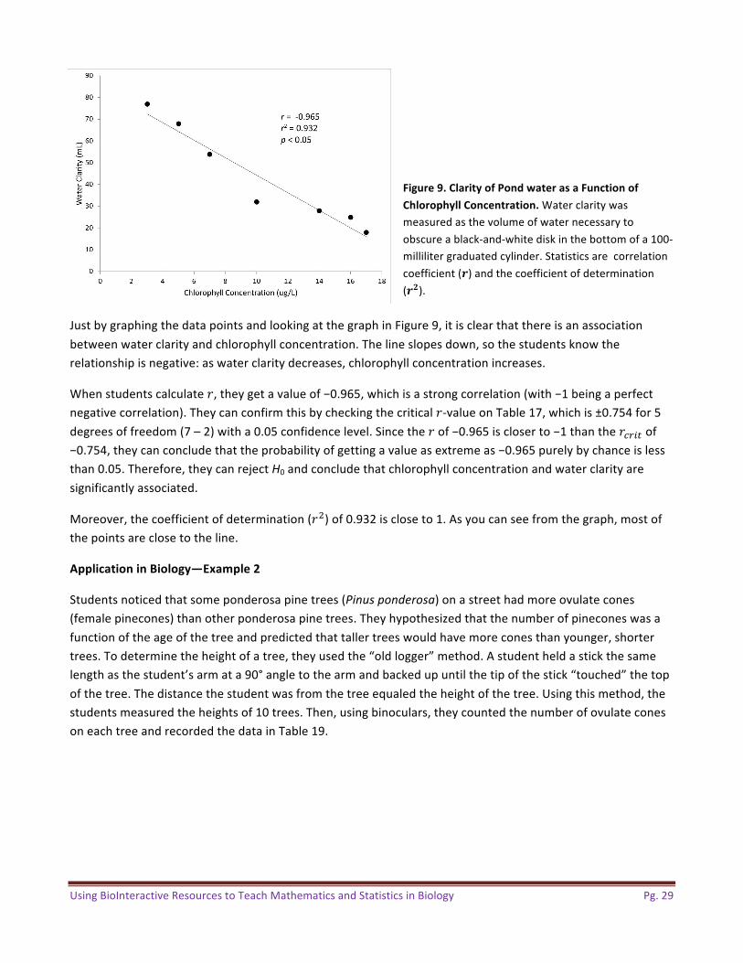
Figure9.ClarityofPondwaterasaFunctionof

ChlorophyllConcentration.Waterclaritywasmeasuredasthevolumeofwaternecessarytoobscureablack-and-whitediskinthebottomofa100-millilitergraduatedcylinder.Statisticsarecorrelationcoefficient(v)andthecoefficientofdetermination(v\).

JustbygraphingthedatapointsandlookingatthegraphinFigure9,itisclearthatthereisanassociationbetweenwaterclarityandchlorophyllconcentration.Thelineslopesdown,sothestudentsknowtherelationshipisnegative:aswaterclaritydecreases,chlorophyllconcentrationincreases.

WhenstudentscalculateA,theygetavalueof−0.965,whichisastrongcorrelation(with−1beingaperfectnegativecorrelation).TheycanconfirmthisbycheckingthecriticalA-valueonTable17,whichis±0.754for5degreesoffreedom(7–2)witha0.05confidencelevel.SincetheAof−0.965iscloserto−1thantheAz{'|of−0.754,theycanconcludethattheprobabilityofgettingavalueasextremeas−0.965purelybychanceislessthan0.05.Therefore,theycanrejectH0andconcludethatchlorophyllconcentrationandwaterclarityaresignificantlyassociated.

Moreover,thecoefficientofdetermination(A.)of0.932iscloseto1.Asyoucanseefromthegraph,mostofthepointsareclosetotheline.


Studentsnoticedthatsomeponderosapinetrees(Pinusponderosa)onastreethadmoreovulatecones(femalepinecones)thanotherponderosapinetrees.Theyhypothesizedthatthenumberofpineconeswasafunctionoftheageofthetreeandpredictedthattallertreeswouldhavemoreconesthanyounger,shortertrees.Todeterminetheheightofatree,theyusedthe“oldlogger”method.Astudentheldastickthesamelengthasthestudent’sarmata90°angletothearmandbackedupuntilthetipofthestick“touched”thetopofthetree.Thedistancethestudentwasfromthetreeequaledtheheightofthetree.Usingthismethod,thestudentsmeasuredtheheightsof10trees.Then,usingbinoculars,theycountedthenumberofovulateconesoneachtreeandrecordedthedatainTable19.


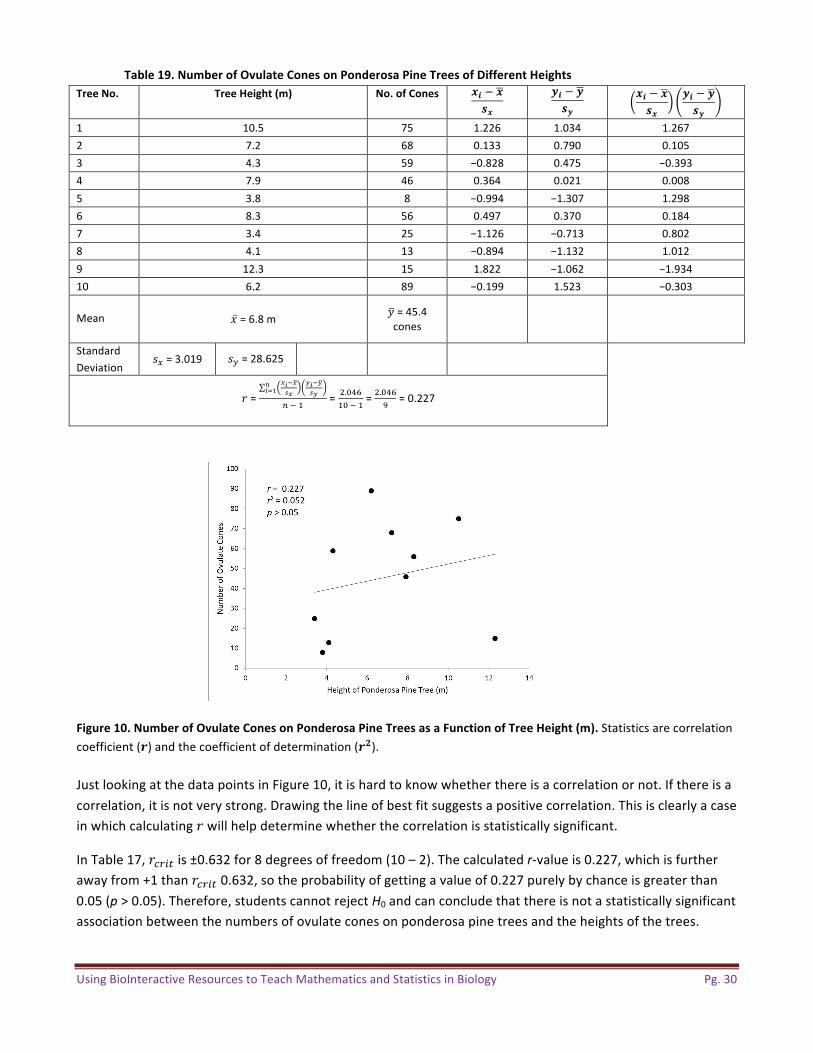
Table19.NumberofOvulateConesonPonderosaPineTreesofDifferentHeights

TreeNo. TreeHeight(m) No.ofCones Z] − ZcZ

w] − wcw

Z] − ZcZ

w] − wcw

1 10.5 75 1.226 1.034 1.2672 7.2 68 0.133 0.790 0.1053 4.3 59 −0.828 0.475 −0.3934 7.9 46 0.364 0.021 0.0085 3.8 8 −0.994 −1.307 1.2986 8.3 56 0.497 0.370 0.1847 3.4 25 −1.126 −0.713 0.8028 4.1 13 −0.894 −1.132 1.0129 12.3 15 1.822 −1.062 −1.93410 6.2 89 −0.199 1.523 −0.303

Mean &=6.8m t=45.4cones

StandardDeviation

-*=3.019 -u=28.625

A=B+CB;B

E+CE;E

<+D:

,02 = ..a`82a02=..a`87 =0.227

Figure10.NumberofOvulateConesonPonderosaPineTreesasaFunctionofTreeHeight(m).Statisticsarecorrelationcoefficient(v)andthecoefficientofdetermination(v\).JustlookingatthedatapointsinFigure10,itishardtoknowwhetherthereisacorrelationornot.Ifthereisacorrelation,itisnotverystrong.Drawingthelineofbestfitsuggestsapositivecorrelation.ThisisclearlyacaseinwhichcalculatingAwillhelpdeterminewhetherthecorrelationisstatisticallysignificant.

InTable17,Az{'|is±0.632for8degreesoffreedom(10–2).Thecalculatedr-valueis0.227,whichisfurtherawayfrom+1thanAz{'|0.632,sotheprobabilityofgettingavalueof0.227purelybychanceisgreaterthan0.05(p>0.05).Therefore,studentscannotrejectH0andcanconcludethatthereisnotastatisticallysignificantassociationbetweenthenumbersofovulateconesonponderosapinetreesandtheheightsofthetrees.


Part3:CommonlyUsedCalculationsinBiology

RelativeFrequencyRelativefrequencyistheratioofthenumberoftimesaneventoccursoutofatotalnumberofevents.Thiscalculatedfractioncanthenbeconvertedintoapercentageofthetotalnumberofeventsmeasured.

relativefrequency=(numberoftimesaspecificeventoccurs)/(totalnumberofevents)

Theresultcanbemultipliedby100togivethepercentage.


Alleleandgenotypefrequenciesarecommonlycalculatedbypopulationgeneticists.Forinstance,inapopulationof350peaplants,suppose112arehomozygousforthedominantyellowpeaseedallele(YY),139areheterozygous(Yy),and99arehomozygousfortherecessivegreenpeaseedallele(yy).

Todeterminetherelativefrequency(andpercentage)ofplantsinthispopulationthatarehomozygousforthedominantyellowpeaseedallele,youshoulddividethenumberofplantsthatarehomozygousfortheyellowpeaseedallelebythetotalnumberofplants:

relativefrequencyofthehomozygousdominant(YY)genotype=112/350=0.32

Toexpressfrequencyasapercentage,multiplythefrequencyby100%:percentage=0.32×100=32%ofthepopulationhasthehomozygousdominantgenotype

Todeterminetherelativefrequency(andpercentage)oftherecessivegreenseedallele,dividethetotalnumberofgreenseedallelesinthegenepoolbythetotalnumberofallelesinthepopulation:

relativefrequencyoftherecessiveallele(y)=[(139×1)+(99×2)]/(350×2)=337/700=0.48percentage=0.48×100=48%ofthegenepoolistherecessivegreenpeaseedallele

ProbabilityYoulearnedinthe“SignificanceTesting”sectionofPart2thataprobabilityof0.05meansthatthereisa5%chanceforaneventtohappen—forexample,a5%chanceofobtainingaparticularteststatisticbychance.Thissectionprovidesmoreinformationaboutprobabilityandhowtocalculateitfordifferentscenarios.

Probabilityallowsscientiststopredictthelikelihoodoftheoutcomeofrandomevents.Probability(p)valuesliebetween1(theeventiscertaintohappen)and0(theeventcertainlywillnothappen).Theprobabilitiesforallothereventshavefractionalvalues.Forexample,theprobabilityofthrowinga2onasix-sideddieis1outof6(p=1/6),sincethenumber2appearsononlyoneofthesixsides.Bycontrast,theprobabilityofthrowinga7onanormalsix-sideddieis0.

RuleofAddition

Theprobabilityofeitheroftwomutuallyexclusiveeventsoccurringisequaltothesumoftheirindividualprobabilities.


Example

Givenanormalsix-sideddie,whatistheprobabilityofyourollingeithera2ora4onthedie?Theseeventsaremutuallyexclusivebecausetheycannothappenatthesametime—thatis,inasinglerollofthedieyoucannotrollbotha2anda4.Thereisa1/6chanceofrollinga2.Thereisa1/6chanceofrollinga4.Theprobabilityofeithereventoccurringisequaltothesumoftheprobabilityofeachevent:

p=1/6+1/6=2/6=1/3

Thereis1chancein3ofyourollingeithera2ora4onthedie.

RuleofMultiplication

Theprobabilityoftwoindependenteventsbothoccurringistheproductoftheirindividualprobabilities.

Example

Givenanormalsix-sideddie,whatistheprobabilityofyourollinga2andthena4ontwoconsecutiverolls?Theseeventsareindependentofoneanotherbecausetheyhavenoeffectoneachother’soccurrence—thatis,ifyourollasix-sideddietwice,rollinga2onthefirstrollhasnoeffectonwhetheryouwillrolla4onthesecondroll.Onthefirstroll,thereisa1/6chanceofrollinga2.Onthesecondroll,thereisa1/6chanceofrollinga4.Theprobabilityofrollinga2firstanda4secondfollows: p=1/6×1/6=1/36Thereis1chancein36ofrollinga2andthena4ontwoconsecutiverollsofthedie.


Whatistheprobabilitythattwoparentswhoareheterozygousforthesicklecellallelewouldhavethreechildreninarowwhoarehomozygousforthesicklecellalleleandhavesicklecellanemia?

Theprobabilityoftwoparentswhoareheterozygousforanalleletohaveachildwhoishomozygousforthatalleleis1in4:

p=1/4×1/4×1/4=1/64Thereis1chancein64thattheseparentswillhavethreechildreninarowwithsicklecelldisease.


Twopeaplantsthatareheterozygousfortheround(R)andyellow(Y)alleles(RrYy)arecrossedandproduceonlyasingleseed.WhatistheprobabilityofaseedfromthiscrosshavingthegenotypeRRYyorRRYY?

TheprobabilityofgettingaseedwiththeRRYygenotypeis1/4×1/2=1/8=2/16.TheprobabilityofgettingaseedwiththeRRYYgenotypeis1/4×1/4=1/16.


ToobtaintheprobabilityofgettingaseedwiththeRRYygenotypeortheRRYYgenotype,weusetheruleofaddition:

p=2/16+1/16=3/16Thereare3chancesin16oftheseplantsproducingaseedwitheithertheRRYyorRRYYgenotype.

RateCalculationsRateisusedtoexpressonemeasuredquantity(y)inrelationtoanothermeasuredquantity(x).

Inbiology,ratesareoftencalculatedtoindicatethechangeinapropertyofasystemovertime.Forexample,therateofanenzyme-catalyzedreactionisfrequentlyexpressedastheamountofproductproducedbytheenzymeinagivenamountoftime.Whenyouusedataplottedonagraph,youcalculatetherateinthesamewayasyoucalculatetheslope:

rate=Δy/Δx

(Thedeltasymbol,Δ,representschange.)ApplicationinBiology

Studentsinanadvancedbiologyclassstudiedthereactioncatalyzedbythecatalaseenzyme.Catalasedegradeshydrogenperoxide(H2O2)towater(H2O)andoxygengas(O2).ThestudentssetupanexperimenttomeasuretheamountofO2producedbycatalaseover5minuteswhenitisaddedtoH2O2.Table20containsthedatacollectedbyagroupofstudents,andFigure11showsthecorrespondinggraph.Fromthesedata,ratesofcatalaseactivitycanbecalculatedovervariousintervalsoftime.

Table20.VolumeofOxygenProducedfromtheCatalysisofHydrogenPeroxidebytheEnzymeCatalase

Time(min.) VolumeofOxygenProduced(mL)

0 01 122 253 334 395 42

Figure11.OxygenProducedinaCatalase-CatalyzedReactionasaFunctionofTime

0

10

20

30

40

50

0 1 2 3 4 5 6

VolumeofOxygen

Produced(mL)

Time(min.)


Tocalculatetheinitialrateofreactioninthefirst2minutesoftheexperiment,studentsfirstsubtractedthevolumeofoxygenproducedat2minutesfromthevolumeofoxygenproducedat0minutes:

Δy=25milliliters–0milliliters=25milliliters

Next,theysubtractedthenumberofminutesat2minutesfromthenumberofminutesat0minutes:

Δx=2minutes–0minutes=2minutes

Finally,theydividedthechangeinoxygenvolume(Δy)bythechangeintime(Δx);thisistherate:

rate=25milliliters/2minutes=12.5millilitersofO2produced/minute

Similarly,theycancalculatetherateofreactionbetweenthethirdandfifthminutesoftheexperiment:

rate=(42milliliters–33milliliters)/(5minutes–3minutes)=9/2=4.5millilitersofO2produced/minute

Hardy-WeinbergFrequencyCalculationsTheHardy-Weinbergequationsareusedinpopulationgeneticstodescribethebasicprinciplethatallelefrequenciesdonotchangeinalarge,freelyinterbreedingpopulationfromonegenerationtothenext.

Allelefrequenciesinapopulationareinequilibrium(donotchange)whenallthefollowingconditionsaremet:

1. Thepopulationisverylargeandwellmixed.2. Thereisnomigrationinoroutofthepopulation.3. Mutationsarenotoccurring.4. Matingisrandom.5. Thereisnonaturalselection.

UnderHardy-Weinberg,ifthefrequenciesoftwoallelesarepandq,thefrequenciesofhomozygotesarep2

andq2,andofheterozygotes2pq.Ifyouaregiventhefrequenciesoftheallelesyoucancalculatedthegenotypefrequenciesbysquaringandmultiplying;ifyouaregivenahomozygousgenotypefrequency,you

canestimatetheallelefrequenciesbytakingthesquareroot.

Hardy-Weinbergpredictsthattheallelefrequenciesinapopulationareatequilibrium,wherebyp+q=1.0

IftheobservedallelefrequenciesinapopulationdifferfromthefrequenciespredictedbytheHardy-Weinbergprinciple,thenthepopulationisnotatequilibriumandevolutionmaybeoccurring.


Inahypotheticalpopulationof100rockpocketmice(Chaetodipusintermedius),81individualshavelight,sandy-coloredfurandaddgenotype.Theremaining19individualsaredarkcoloredandthereforehaveeithertheDDgenotypeortheDdgenotype.Scientistsassumedthatthispopulationisatequilibrium;theyusedtheHardy-Weinbergequationstofindpandqforthispopulationandcalculatedthefrequencyofheterozygousgenotypes.


Scientistsknewthat81micehavetheddgenotype:q2=81/100=0.81,or81%

Next,theycalculatedq:

q= 0.81=0.9

Then,theycalculatedpusingtheequationp+q=1:

p+(0.9)=1p=0.1

Tocalculatethefrequencyoftheheterozygousgenotype,theycalculated2pq:

2pq=2(0.1)(0.9)=2(0.09)2pq=0.18

Basedonthecalculations,theestimatedfrequencyoftherecessivealleleis0.9andthefrequencyofthedominantalleleis0.1.

Ifthescientistshadawaytodistinguishmicethatareheterozygotesfromthosethatarehomozygousdominantforthedark-coloredfur,thentheywouldhaveawayofdeterminingwhetherthepopulationisorisnotatequilibriumandcouldapplyastatisticaltestlikethechi-squaretesttoseeifthereisadifference.

StandardCurvesAstandardcurveisamethodofquantitativedataanalysisinwhichmeasurementsofsampleswithknownpropertiesareplottedonagraphandthenthegraphisanalyzedtodeterminethepropertiesofunknownsamples.Analysisofthegraphisperformedbydrawingalineofbestfitthroughtheplottedpointsoftheknownsamplesandthendeterminingtheequationofthisline(intheformy=mx+b)orbyinterpretingthevaluesofunknownsamplesdirectlyfromthedrawnline.Thesampleswithknownpropertiesarethestandards,andthegraphisthestandardcurve.TwocommonusesofstandardcurvesinbiologyaretodetermineproteinconcentrationsandtoanalyzeDNAfragmentlength.

ApplicationinBiology—Example1:TheBradfordProteinAssay

TheBradfordproteinassayisacolorimetricassaythatdeterminestheproteinconcentrationofasolutionbymeasuringhowmuchlightofacertainwavelengthitabsorbs.Thelightabsorbanceofseveralsampleswithknownproteinconcentrationsismeasuredusingaspectrophotometerandthenplottedonagraphasafunctionofproteinconcentration.Usingthisgraph,orlinearregressionanalysis,scientistsdeterminedtheproteinconcentrationofanunknownsampleonceitsabsorbancewasmeasured.

Table21.AbsorbanceMeasuredat595NanometersofVariousKnownProteinConcentrations

KnownProtein

Concentration(µg/mL)

MeasuredAbsorbance(at

595nm)

1 0.4335 0.74210 1.03615 1.46320 1.750


Figure12.ProteinConcentrationasaFunctionofAbsorbance

InFigure12,absorbanceinTable21wasplottedasafunctionofproteinconcentrationfortheknownsamples(standards).Thecalculatedcoefficientofdetermination(A.)andequationoftheregressionlineareincludedonthegraph.TheclosertheA.valueisto1,thebetterthedatafitthecurve—orthemorelikelythatthedatapointsxandyareactualsolutionstotheequationy=mx+b.

Inthiscase,theequationofthelineis

y=0.0699x+0.3722

Theabsorbanceoftheunknownproteinsolutionwasmeasuredwithaspectrophotometeras0.921(y=0.921),sothescientistsusedtheequationofthebest-fitlinetodeterminetheproteinconcentration(x):

0.921=0.0699x+0.3722

Proteinconcentrationofunknown:x=7.85microgramspermilliliter

TheredlinesdrawnonthegraphinFigure12showhowthescientistsestimatedthevalueoftheunknownproteinconcentrationfromtheregressionline.Todeterminethisestimate,theylocatedtheabsorbanceof0.921onthey-axisandtracedithorizontallytoitsintersectionwiththeregressionline.Averticallinefromtheintersectionwillcrossthex-axisatthecorrespondingproteinconcentration.

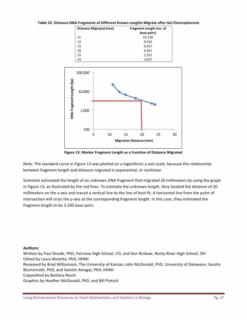
ApplicationinBiology—Example2:DNAFragmentSizeAnalysis

InRFLP(restrictionfragmentlengthpolymorphism)analysis,thefragmentsizesofunknownDNAsamplescanbedeterminedfromthestandardcurveofDNAmarkersofknownfragmentlengths.First,scientistsmeasuredthedistancetraveledbyeachofthemarkerfragmentsinagelplateandplotteditasafunctionofsize.Thisprovidesastandardforcomparisontointerpolatethesizeoftheunknownfragments(Table22).

y =0.0699x +0.3722r²=0.9965

0

0.5

1

1.5

2

0 5 10 15 20 25

Absorbance(at595nm)

ProteinConcentration(μg/mL)


Table22.DistanceDNAFragmentsofDifferentKnownLengthsMigrateafterGelElectrophoresis

DistanceMigrated(mm) FragmentLength(no.of

basepairs)

11 23,13013 9,41615 6,55718 4,36123 2,32224 2,027

Figure13.MarkerFragmentLengthasaFunctionofDistanceMigrated

Note:ThestandardcurveinFigure13wasplottedonalogarithmicy-axisscale,becausetherelationshipbetweenfragmentlengthanddistancemigratedisexponential,ornonlinear.

ScientistsestimatedthelengthofanunknownDNAfragmentthatmigrated20millimetersbyusingthegraphinFigure13,asillustratedbytheredlines.Toestimatetheunknownlength,theylocatedthedistanceof20millimetersonthex-axisandtracedaverticallinetothelineofbestfit.Ahorizontallinefromthepointofintersectionwillcrossthey-axisatthecorrespondingfragmentlength.Inthiscase,theyestimatedthefragmentlengthtobe3,100basepairs.

Authors:

WrittenbyPaulStrode,PhD,FairviewHighSchool,CO,andAnnBrokaw,RockyRiverHighSchool,OHEditedbyLauraBonetta,PhD,HHMIReviewedbyBradWilliamson,TheUniversityofKansas;JohnMcDonald,PhD,UniversityofDelaware;SandraBlumenrath,PhD,andSatoshiAmagai,PhD,HHMICopyeditedbyBarbaraReschGraphicsbyHeatherMcDonald,PhD,andBillPietsch

100

1,000

10,000

100,000

5 10 15 20 25 30

DNAFragmentLength(bp)

MigrationDistance(mm)


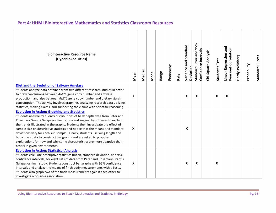
Part4:HHMIBioInteractiveMathematicsandStatisticsClassroomResources

BioInteractiveResourceName

(HyperlinkedTitles)

Mean

Median

Mode

Range

Frequency

Rate

VarianceandStandard

Deviation

StandardErrorand95%

ConfidenceIntervals

Chi-SquareAnalysis

Studentt-Test

LinearRegressionand

Pearson’sCorrelation

Hardy-W

einberg

Probability

StandardCurves

DietandtheEvolutionofSalivaryAmylaseStudentsanalyzedataobtainedfromtwodifferentresearchstudiesinordertodrawconclusionsbetweenAMY1genecopynumberandamylaseproduction;andalsobetweenAMY1genecopynumberanddietarystarchconsumption.Theactivityinvolvesgraphing,analyzingresearchdatautilizingstatistics,makingclaims,andsupportingtheclaimswithscientificreasoning.

X X X X X

EvolutioninAction:GraphingandStatisticsStudentsanalyzefrequencydistributionsofbeakdepthdatafromPeterandRosemaryGrant’sGalapagosfinchstudyandsuggesthypothesestoexplainthetrendsillustratedinthegraphs.Studentstheninvestigatetheeffectofsamplesizeondescriptivestatisticsandnoticethatthemeansandstandarddeviationsvaryforeachsubsample.Finally,studentsusewinglengthandbodymassdatatoconstructbargraphsandareaskedtoproposeexplanationsforhowandwhysomecharacteristicsaremoreadaptivethanothersingivenenvironments.

X X

EvolutioninAction:StatisticalAnalysisStudentscalculatedescriptivestatistics(mean,standarddeviation,and95%confidenceintervals)foreightsetsofdatafromPeterandRosemaryGrant’sGalapagosfinchstudy.Studentsconstructbargraphswith95%confidenceintervalsandanalyzethemeansoffinchbodymeasurementswitht-Tests.Studentsalsographtwoofthefinchmeasurementsagainsteachothertoinvestigateapossibleassociation.

X X X X



(HyperlinkedTitles)

Mean

Median

Mode

Range

Frequency

Rate

VarianceandStandard

Deviation

StandardErrorand95%

ConfidenceIntervals

Chi-SquareAnalysis

Studentt-Test

LinearRegressionand


Hardy-W

einberg

Probability

StandardCurves

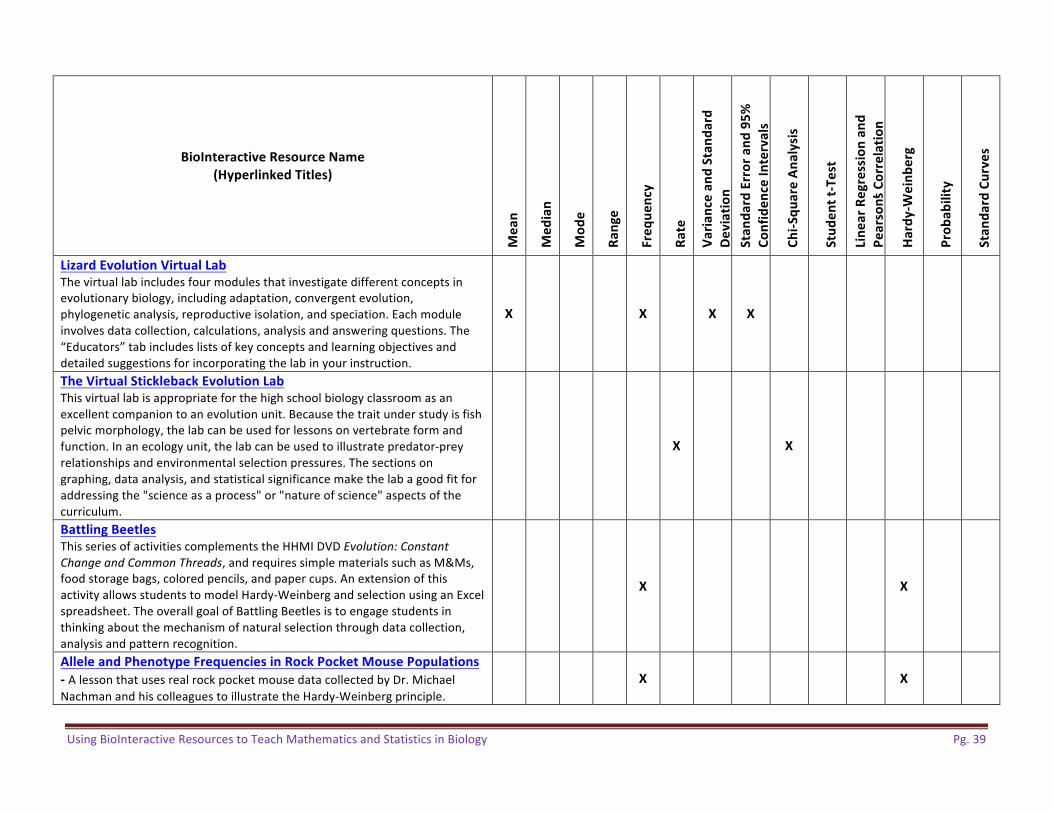
LizardEvolutionVirtualLabThevirtuallabincludesfourmodulesthatinvestigatedifferentconceptsinevolutionarybiology,includingadaptation,convergentevolution,phylogeneticanalysis,reproductiveisolation,andspeciation.Eachmoduleinvolvesdatacollection,calculations,analysisandansweringquestions.The“Educators”tabincludeslistsofkeyconceptsandlearningobjectivesanddetailedsuggestionsforincorporatingthelabinyourinstruction.

X X X X

TheVirtualSticklebackEvolutionLabThisvirtuallabisappropriateforthehighschoolbiologyclassroomasanexcellentcompaniontoanevolutionunit.Becausethetraitunderstudyisfishpelvicmorphology,thelabcanbeusedforlessonsonvertebrateformandfunction.Inanecologyunit,thelabcanbeusedtoillustratepredator-preyrelationshipsandenvironmentalselectionpressures.Thesectionsongraphing,dataanalysis,andstatisticalsignificancemakethelabagoodfitforaddressingthe"scienceasaprocess"or"natureofscience"aspectsofthecurriculum.

X X

BattlingBeetlesThisseriesofactivitiescomplementstheHHMIDVDEvolution:ConstantChangeandCommonThreads,andrequiressimplematerialssuchasM&Ms,foodstoragebags,coloredpencils,andpapercups.AnextensionofthisactivityallowsstudentstomodelHardy-WeinbergandselectionusinganExcelspreadsheet.TheoverallgoalofBattlingBeetlesistoengagestudentsinthinkingaboutthemechanismofnaturalselectionthroughdatacollection,analysisandpatternrecognition.

X X

AlleleandPhenotypeFrequenciesinRockPocketMousePopulations

-AlessonthatusesrealrockpocketmousedatacollectedbyDr.MichaelNachmanandhiscolleaguestoillustratetheHardy-Weinbergprinciple.

X X



(HyperlinkedTitles)

Mean

Median

Mode

Range

Frequency

Rate

VarianceandStandard

Deviation

StandardErrorand95%

ConfidenceIntervals

Chi-SquareAnalysis

Studentt-Test

LinearRegressionand


Hardy-W

einberg

Probability

StandardCurves

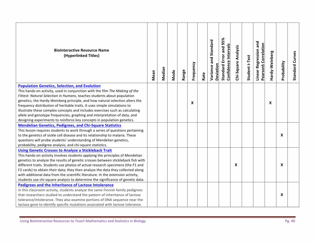
PopulationGenetics,Selection,andEvolutionThishands-onactivity,usedinconjunctionwiththefilmTheMakingoftheFittest:NaturalSelectioninHumans,teachesstudentsaboutpopulationgenetics,theHardy-Weinbergprinciple,andhownaturalselectionaltersthefrequencydistributionofheritabletraits.Itusessimplesimulationstoillustratethesecomplexconceptsandincludesexercisessuchascalculatingalleleandgenotypefrequencies,graphingandinterpretationofdata,anddesigningexperimentstoreinforcekeyconceptsinpopulationgenetics.

X X

MendelianGenetics,Pedigrees,andChi-SquareStatisticsThislessonrequiresstudentstoworkthroughaseriesofquestionspertainingtothegeneticsofsicklecelldiseaseanditsrelationshiptomalaria.Thesequestionswillprobestudents'understandingofMendeliangenetics,probability,pedigreeanalysis,andchi-squarestatistics.

X

UsingGeneticCrossestoAnalyzeaSticklebackTraitThishands-onactivityinvolvesstudentsapplyingtheprinciplesofMendeliangeneticstoanalyzetheresultsofgeneticcrossesbetweensticklebackfishwithdifferenttraits.Studentsusephotosofactualresearchspecimens(theF1andF2cards)toobtaintheirdata;theythenanalyzethedatatheycollectedalongwithadditionaldatafromthescientificliterature.Intheextensionactivity,studentsusechi-squareanalysistodeterminethesignificanceofgeneticdata.

X X

PedigreesandtheInheritanceofLactoseIntoleranceInthisclassroomactivity,studentsanalyzethesameFinnishfamilypedigreesthatresearchersstudiedtounderstandthepatternofinheritanceoflactosetolerance/intolerance.TheyalsoexamineportionsofDNAsequencenearthelactasegenetoidentifyspecificmutationsassociatedwithlactosetolerance.

X



(HyperlinkedTitles)

Mean

Median

Mode

Range

Frequency

Rate

VarianceandStandard

Deviation

StandardErrorand95%

ConfidenceIntervals

Chi-SquareAnalysis

Studentt-Test

LinearRegressionand


Hardy-W

einberg

Probability

StandardCurves

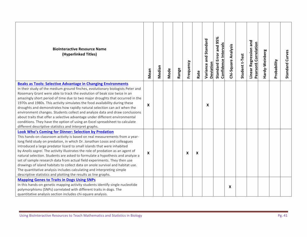
BeaksasTools:SelectiveAdvantageinChangingEnvironmentsIntheirstudyofthemediumgroundfinches,evolutionarybiologistsPeterandRosemaryGrantwereabletotracktheevolutionofbeaksizetwiceinanamazinglyshortperiodoftimeduetotwomajordroughtsthatoccurredinthe1970sand1980s.Thisactivitysimulatesthefoodavailabilityduringthesedroughtsanddemonstrateshowrapidlynaturalselectioncanactwhentheenvironmentchanges.Studentscollectandanalyzedataanddrawconclusionsabouttraitsthatofferaselectiveadvantageunderdifferentenvironmentalconditions.TheyhavetheoptionofusinganExcelspreadsheettocalculatedifferentdescriptivestatisticsandinterpretgraphs.

X X

LookWho’sComingforDinner:SelectionbyPredationThishands-onclassroomactivityisbasedonrealmeasurementsfromayear-longfieldstudyonpredation,inwhichDr.JonathanLososandcolleaguesintroducedalargepredatorlizardtosmallislandsthatwereinhabitedbyAnolissagrei.Theactivityillustratestheroleofpredationasanagentofnaturalselection.Studentsareaskedtoformulateahypothesisandanalyzeasetofsampleresearchdatafromactualfieldexperiments.Theythenusedrawingsofislandhabitatstocollectdataonanolesurvivalandhabitatuse.Thequantitativeanalysisincludescalculatingandinterpretingsimpledescriptivestatisticsandplottingtheresultsaslinegraphs.

X X X

MappingGenestoTraitsinDogsUsingSNPsInthishands-ongeneticmappingactivitystudentsidentifysinglenucleotidepolymorphisms(SNPs)correlatedwithdifferenttraitsindogs.Thequantitativeanalysissectionincludeschi-squareanalysis.

X



(HyperlinkedTitles)

Mean

Median

Mode

Range

Frequency

Rate

VarianceandStandard

Deviation

StandardErrorand95%

ConfidenceIntervals

Chi-SquareAnalysis

Studentt-Test

LinearRegressionand


Hardy-W

einberg

Probability

StandardCurves

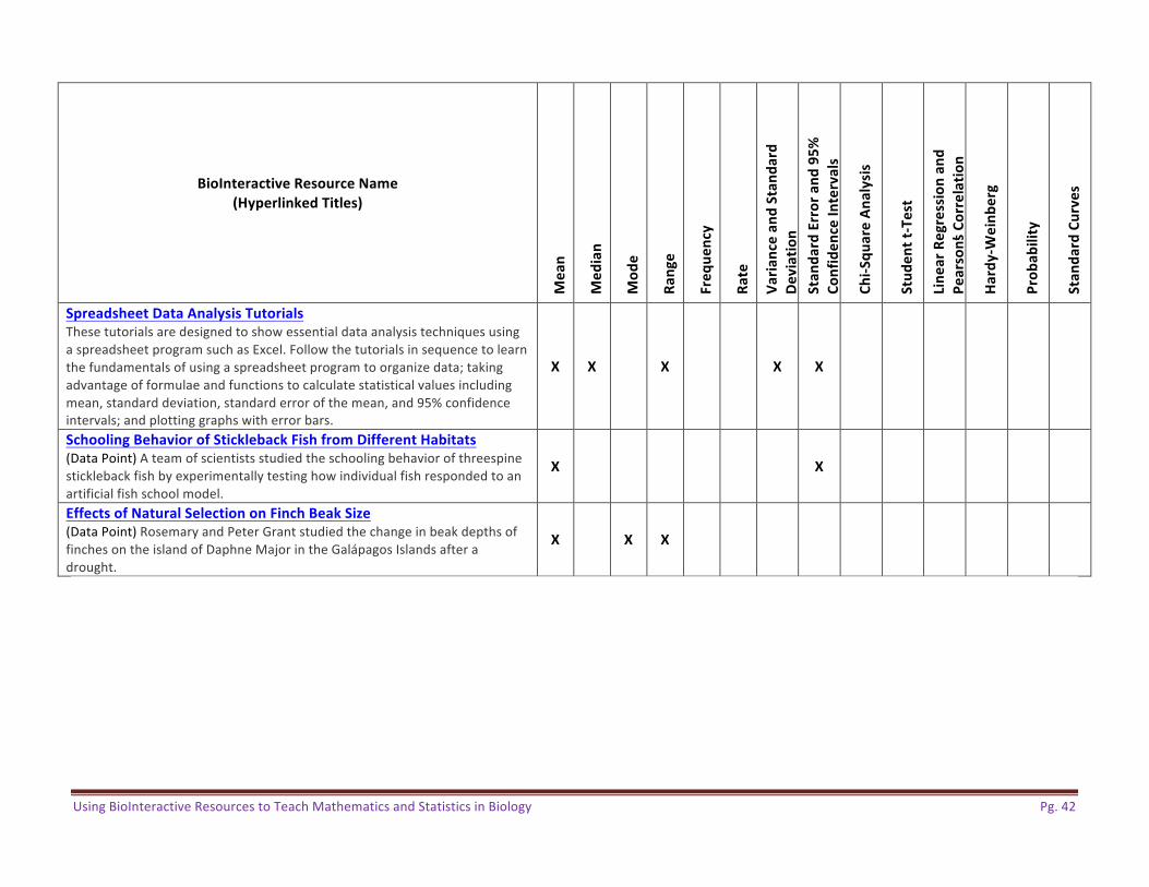
SpreadsheetDataAnalysisTutorialsThesetutorialsaredesignedtoshowessentialdataanalysistechniquesusingaspreadsheetprogramsuchasExcel.Followthetutorialsinsequencetolearnthefundamentalsofusingaspreadsheetprogramtoorganizedata;takingadvantageofformulaeandfunctionstocalculatestatisticalvaluesincludingmean,standarddeviation,standarderrorofthemean,and95%confidenceintervals;andplottinggraphswitherrorbars.

X X X X X

SchoolingBehaviorofSticklebackFishfromDifferentHabitats(DataPoint)Ateamofscientistsstudiedtheschoolingbehaviorofthreespinesticklebackfishbyexperimentallytestinghowindividualfishrespondedtoanartificialfishschoolmodel.

X X

EffectsofNaturalSelectiononFinchBeakSize(DataPoint)RosemaryandPeterGrantstudiedthechangeinbeakdepthsoffinchesontheislandofDaphneMajorintheGalápagosIslandsafteradrought.

X X X

Mathematics and Statistics in...

Documents

Transcript of Mathematics and Statistics in...