Mathematical Principles in Vision and Graphics: Projective ... · Mathematical Principles in Vision...
27
Mathematical Principles in Vision and Graphics: Projective Geometry – Part 2 Ass.Prof. Friedrich Fraundorfer SS 2019 1
Transcript of Mathematical Principles in Vision and Graphics: Projective ... · Mathematical Principles in Vision...

Mathematical Principles in Vision and
Graphics:
Projective Geometry – Part 2
Ass.Prof. Friedrich Fraundorfer
SS 2019
1

Outline
Axioms of geometry
Differences between Euclidean and projective geometry
2D projective geometry
▫ Homogeneous coordinates
▫ Points, Lines
▫ Duality
3D projective geometry
▫ Points, Lines, Planes
▫ Duality
▫ Plane at infinity
▫ Image formation
▫ Parameterizing a camera matrix
▫ Projection of points and lines
Geometric relationships
▫ Epipolar constraint derivation
▫ Stereo normal case
▫ Triangulation
▫ Camera pose estimation (algebraic, from points and lines)
2
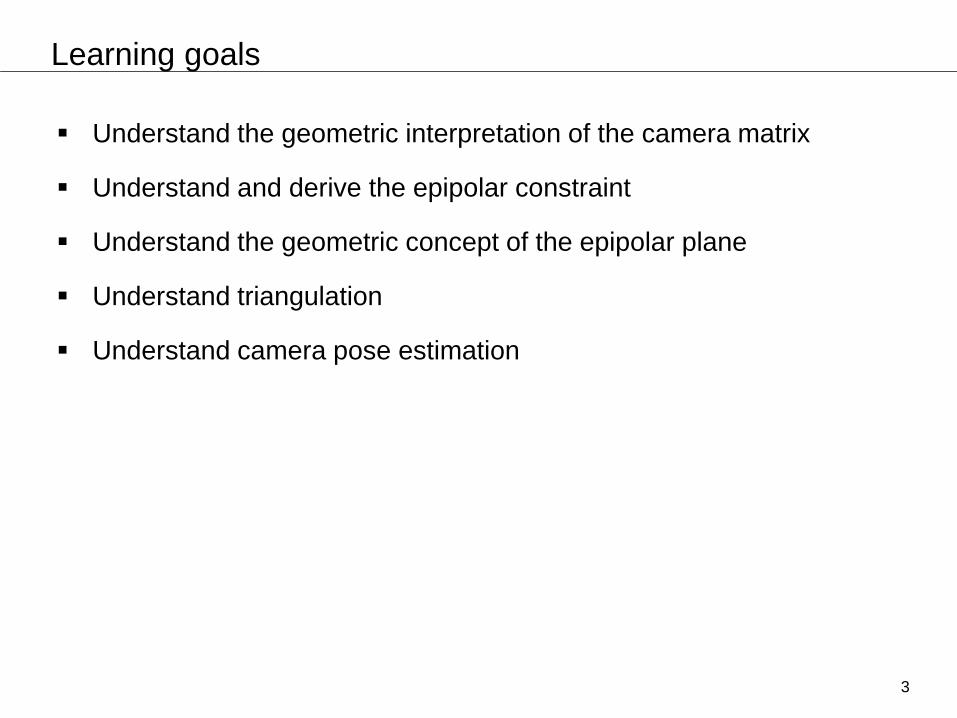
Learning goals
Understand the geometric interpretation of the camera matrix
Understand and derive the epipolar constraint
Understand the geometric concept of the epipolar plane
Understand triangulation
Understand camera pose estimation
3

Camera matrix (calibrated camera)
Camera matrix is a coordinate transformation and then a projection
C … 3x1 coordinate of the camera center in world coordinate
R … 3x3 rotation matrix representing the orientation of the camera
coordinate frame
K … 3x3 calibration matrix
𝑃 = 𝐾𝑅 𝐼 −𝐶 = 𝐾 𝑅 −𝑅𝐶 = 𝐾 𝑅 𝑡𝑡 = −𝑅𝐶
4
O
Z
Y
X
R,t
Zcam
Ycam
Xcam
C

Geometric interpretation of camera matrix entries
Columns (3x1 vectors) are unit vectors of the coordinate system
Rows transposed (1x4 vectors) are planes spanned by coordinate
system axis
𝑃 =
𝑝11𝑝21𝑝31
𝑝12𝑝22𝑝32
𝑝13𝑝23𝑝33
𝑝14𝑝24𝑝34
= 𝑝1 𝑝2 𝑝3 𝑝4 =
𝑃1𝑇
𝑃2𝑇
𝑃3𝑇
5

Geometric interpretation of camera matrix entries
p1,p2,p3 are the images of the axis directions (vanishing points)
x-axis … D=(1,0,0,0) is imaged as p1=PD
6
CO
Z
Y
X
p1
p3
p2

Geometric interpretation of camera matrix entries
𝑃3𝑇 is the principal plane, the plane parallel to the image plane through
the camera center
𝑃𝑋 = (𝑥, 𝑦, 0) all points on the principal plane have the following
coordinates
Plane condition, 𝑃3𝑇𝑋 = 0 (point X is on the plane if it fulfils the
condition)
Points on P2, 𝑃2𝑇𝑋 = 0, all points have coordinates 𝑃𝑋 = (𝑥, 0, 𝑧)
Plane P2 is defined by the line y=0 and the camera center
7
C
P2
yx
C
P3y
x
principal plane
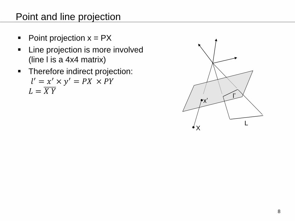
Point and line projection
Point projection x = PX
Line projection is more involved
(line l is a 4x4 matrix)
Therefore indirect projection:
𝑙′ = 𝑥′ × 𝑦′ = 𝑃𝑋 × 𝑃𝑌𝐿 = 𝑋 𝑌
8
LX
x’l’

Epipolar constraint
An image point x lies on its corresponding epipolar line in the
corresponding image.
9
pp’
x’x
X world point
CC’t
[R|t]
X1
X2
X3
e’e
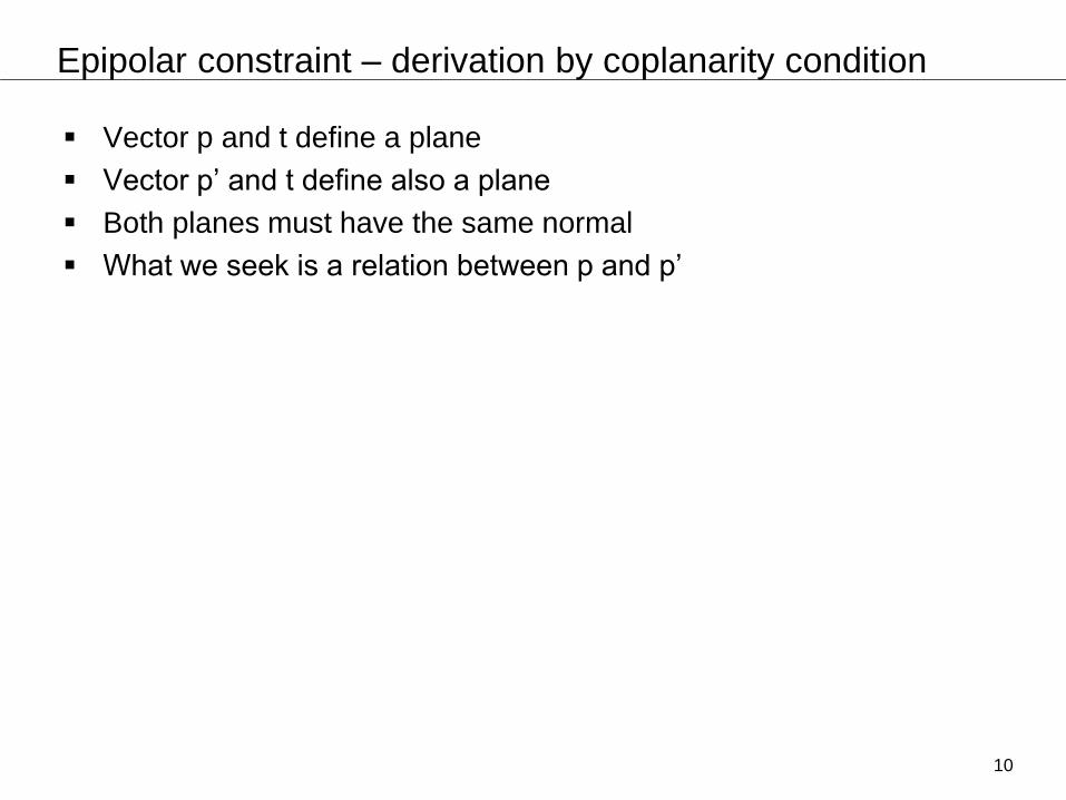
Epipolar constraint – derivation by coplanarity condition
Vector p and t define a plane
Vector p’ and t define also a plane
Both planes must have the same normal
What we seek is a relation between p and p’
10
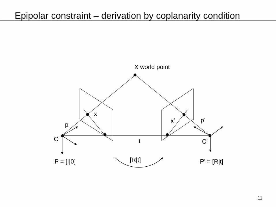
Epipolar constraint – derivation by coplanarity condition
11
pp’x’
x
X world point
C C’t
[R|t] P’ = [R|t]P = [I|0]

Epipolar constraint – derivation by coplanarity condition
pp’x’
x
X world point
C C’t
[R|t]
12
(t x p’)

Epipolar constraint – derivation by coplanarity condition
pp’x’
x
X world point
C C’t
[R|t]
13
(t x p’)

Epipolar constraint – derivation by coplanarity condition
14
pp’x’
x
X world point
C C’t
[R|t]
p’’=Rp+t(t x p’)

Epipolar constraint – derivation by coplanarity condition
𝑡 × 𝑝′ = 𝑡 × 𝑝′′
𝑡 × 𝑝′ = 𝑡 × 𝑅𝑝 + 𝑡𝑤𝑖𝑡ℎ 𝑝′′ = 𝑅𝑝 + 𝑡𝑡 × 𝑝′ = 𝑡 × 𝑅𝑝 + 𝑡 × 𝑡
𝑝′𝑇𝑡 × 𝑝′ = 0
𝑝′𝑇𝑡 × 𝑅𝑝 = 0
𝑝′𝑇[𝑡]𝑥𝑅𝑝 = 0
𝐸
𝑝′𝑇𝐸𝑝 = 0
E is called the Essential matrix 15
pp’x’
x
X world point
C C’t
[R|t]
p’’=Rp+t(t x p’)

Fundamental matrix
p,p’ from the Essential matrix derivation are in normalized coordinates
x,x’ are image coordinates, x=Kp, x’=Kp
By replacing p,p’ with x,x’ one gets the Fundamental matrix
16
𝑝′𝑇𝐸𝑝 = 0
𝑥′𝑇𝐾−𝑇𝐸𝐾−1𝑥 = 0
𝑥′𝑇𝐹𝑥 = 0
F = 𝐾−𝑇𝐸𝐾−1

Epipolar lines
The corresponding line l’ to image coordinate x
l’ is the line connecting the epipole e’ and the image coordinate x’
Hypothesis: 𝑙′ = 𝐹𝑥
Point x’ must lie on l’, thus 𝑥′𝑇𝑙′ = 0
Now 𝑥′𝑇𝐹𝑥 = 0
17
pp’x’
x
X world point
C C’t
[R|t] P’ = [R|t]P = [I|0]
l’

Stereo case
p
x’
x
X world point
C
C’
𝑅 = 𝐼3𝑥3 𝑇 = [𝑇𝑥 0 0] 𝑇
18

Stereo case
p
x’
x
X world point
C
C’
𝑅 = 𝐼3𝑥3 𝑇 = [𝑇𝑥 0 0] 𝑇
𝐸 = [𝑇]𝑥𝑅 =0 0 00 0 −𝑇𝑥0 𝑇𝑥 0
𝑥′ 𝑦′ 10 0 00 0 −𝑇𝑥0 𝑇𝑥 0
𝑥𝑦1
= 0
𝑥′ 𝑦′ 10
−𝑇𝑥𝑇𝑥𝑦
= 0
−𝑦′𝑇𝑥 + 𝑇𝑥𝑦 = 0
19

Triangulation
Compute coordinates of world point X given the measurements x, x’ and
the camera projection matrices P and P’
pp’x’
x
X world point
C C’
20

Triangulation
Condition: Measurement vector x needs to have the same direction as
projection of X (cross-product equals 0)
𝑥 × 𝑃𝑋 = 0 𝑎𝑛𝑑 𝑥′ × 𝑃′𝑋 = 0
Can be rewritten into equation system 𝐴𝑋 = 0 to solve for X
pp’x’
x
X world point
C C’
21

Triangulation
x’x
X world point
C C’
22
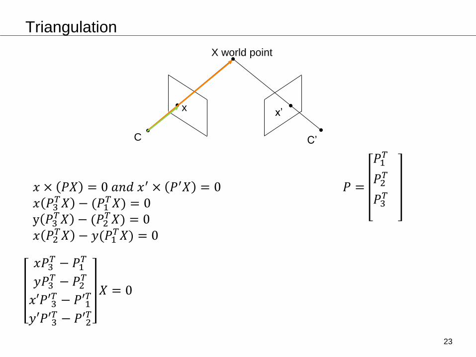
Triangulation
x’x
X world point
C C’
𝑃 =
𝑃1𝑇
𝑃2𝑇
𝑃3𝑇
𝑥 × 𝑃𝑋 = 0 𝑎𝑛𝑑 𝑥′ × 𝑃′𝑋 = 0𝑥 𝑃3
𝑇𝑋 − (𝑃1𝑇𝑋) = 0
y 𝑃3𝑇𝑋 − (𝑃2
𝑇𝑋) = 0𝑥 𝑃2
𝑇𝑋 − 𝑦(𝑃1𝑇𝑋) = 0
𝑥𝑃3𝑇 − 𝑃1
𝑇
𝑦𝑃3𝑇 − 𝑃2
𝑇
𝑥′𝑃′3𝑇 − 𝑃′1
𝑇
𝑦′𝑃′3𝑇 − 𝑃′2
𝑇
𝑋 = 0
23
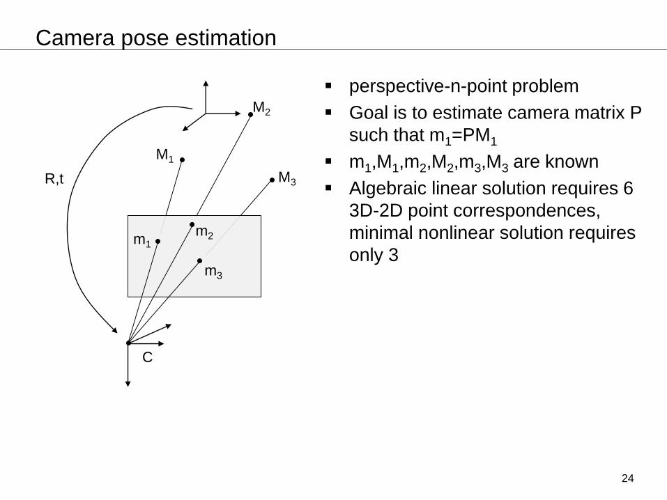
Camera pose estimation
perspective-n-point problem
Goal is to estimate camera matrix P
such that m1=PM1
m1,M1,m2,M2,m3,M3 are known
Algebraic linear solution requires 6
3D-2D point correspondences,
minimal nonlinear solution requires
only 3
24
R,t
C
M1
M2
m1
M3
m2
m3

R,t
C
M1
M2
m1
M3
m2
m3
Camera pose estimation
Derivation similar to Triangulation,
but now entries of P are the
unknowns instead of X
Condition: Measurement vector x
needs to have the same direction as
projection of X (cross-product equals
0)
25

R,t
C
M1
M2
m1
M3
m2
m3
Camera pose estimation
Derivation similar to Triangulation,
bot now entries of P are the
unknowns instead of X
Condition: Measurement vector x
needs to have the same direction as
projection of X (cross-product equals
0)
𝑥 × 𝑃𝑋 = 0 𝑓𝑜𝑟 𝑎𝑙𝑙 𝑝𝑎𝑖𝑟𝑠 𝑥 ⟷ 𝑋y 𝑃3
𝑇𝑋 − 𝑤(𝑃2𝑇𝑋) = 0
𝑥 𝑃3𝑇𝑋 − 𝑤(𝑃1
𝑇𝑋) = 0𝑥 𝑃2
𝑇𝑋 − 𝑦(𝑃1𝑇𝑋) = 0
0 −𝑤𝑋𝑇 𝑦𝑋𝑇
−𝑤𝑋𝑇 0 𝑥𝑋𝑇
−𝑦𝑋𝑇 𝑥𝑋𝑇 0
𝑃1
𝑃2
𝑃3
= 0
26

Recap - Learning goals
Understand the geometric interpretation of the camera matrix
Understand and derive the epipolar constraint
Understand the geometric concept of the epipolar plane
Understand triangulation
Understand camera pose estimation
27