Mathematical Modelling Lecture 4 -- Fitting Datapjh503/mathematical_model/math_model4.pdf · Data...

Data fittingModel fitting

Least-squaresComparing models

Mathematical ModellingLecture 4 – Fitting Data

Phil [email protected]

Phil Hasnip Mathematical Modelling



Overview of Course

Model construction −→ dimensional analysisExperimental input −→ fittingFinding a ‘best’ answer −→ optimisationTools for constructing and manipulating models −→networks, differential equations, integrationTools for constructing and simulating models −→randomnessReal world difficulties −→ chaos and fractals

A First Course in Mathematical Modeling by Giordano, Weir &Fox, pub. Brooks/Cole. Today we’re in chapter 3.




Aim

There are two main aims:

To fit a model to experimental data, or to choose whichmodel best fits the data −→ Model fitting.To use given experimental data with a model to predictother experimental results −→ Model interpolation.




Aim

The difference between these two aims is one of emphasis:

Model fitting: we expect some scatter in the experimentaldata, we want the best model of a given form – ‘theorydriven’Model interpolation: the existing data is good, model isless important – ‘data driven’

Today we’ll be focussing on the first aim: model fitting.




Model fitting

What do we mean by model fit-ting? Suppose we know

f (x) = a + bx + cx2

If we knew f (x) at three differentpoints precisely then we couldcompute a, b and c.




Model fitting

In practice there is always ex-perimental error, so we makeseveral measurements and tryto find the values of a, b and cthat fit the data best. How do wedo that?




Least-squares

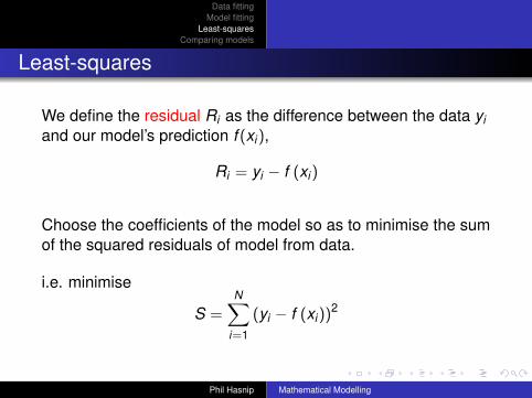
We define the residual Ri as the difference between the data yiand our model’s prediction f (xi),

Ri = yi − f (xi)

Choose the coefficients of the model so as to minimise the sumof the squared residuals of model from data.

i.e. minimise

S =N∑

i=1

(yi − f (xi))2




Least-squares

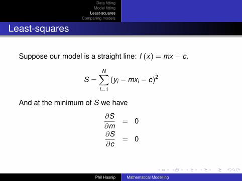
Suppose our model is a straight line: f (x) = mx + c.

S =N∑

i=1

(yi −mxi − c)2

And at the minimum of S we have

∂S∂m

= 0

∂S∂c

= 0




Least-squares

m =N

∑Ni=1 xiyi −

(∑Ni=1 xi

) (∑Ni=1 yi

)N

∑Ni=1 x2

i −(∑N

i=1 xi

)2

c =

(∑Ni=1 x2

i

) (∑Ni=1 yi

)−

(∑Ni=1 xiyi

) (∑Ni=1 xi

)N

∑Ni=1 x2

i −(∑N

i=1 xi

)2

Similar process for other forms of f (xi), though moreparameters!




Least-squares

S =N∑

i=1

(yi − f (xi))2

S measures the absolute error, but we could also measure therelative error:

SR =N∑

i=1

(yi − f (xi))2

f (xi)2

These are both closely related to χ2, another measure of‘goodness of fit’:

χ2 =N∑

i=1

(yi − f (xi))2

f (xi)




Data transformations

What about transforming the data? E.g.

y = αeβx

⇒ ln y = ln α + βx

we could then fit a straight line to ln y .

Not a good idea! See spreadsheet...




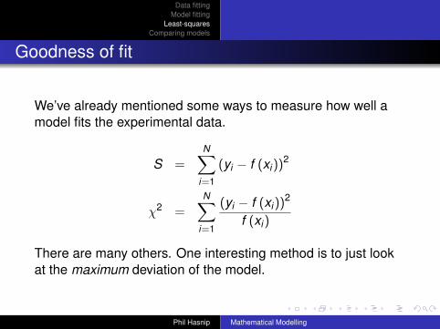
Goodness of fit

We’ve already mentioned some ways to measure how well amodel fits the experimental data.

S =N∑

i=1

(yi − f (xi))2

χ2 =N∑

i=1

(yi − f (xi))2

f (xi)

There are many others. One interesting method is to just lookat the maximum deviation of the model.




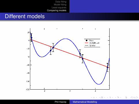
Different models

Once we have decided on our measure of ‘goodness of fit’, wecan decide which of several models is the best.

BUT we need to be careful...




Different models




Different models

A model with more parameters is much more likely to fit thedata well, regardless of whether it is actually better or not.

Adding another term to a model usually improves the fitIs this improvement ‘real’, or chance?Is it worth adding the extra parameter?Occam’s razor −→ simpler is better!




Degrees of freedom

If N data points, and p model parameters, then can think of thefitting process as:

Use first p data points to determine model parametersUse remaining N − p points to calculate error

The N − p points represent the freedom we have in fitting amodel of this form. We say there are N − p degrees of freedom.




F-test

We look at the fractional improvement in goodness of fit, andwe do this by calculating F ,

F =χ2

2

χ21

(label models such that F ≥ 1).

What F could just be chance? Decide what probability to reject:e.g. if probability of F by chance is ≤ 5% then it is unlikely tohappen accidentally, so decide model 2 is better than model 1.

The probability we choose to reject (e.g. 5%) is called thesignificance level – we usually use 5% or 1%.




Critical F-values

The maximum likely improvement of F due to chance at varioussignificance levels can be found in tables of F values. Itdepends on the degrees of freedom of each model, so ourprocedure for testing is:

Work out degrees of freedom for each modelDecide significance level (usually 5% or 1%)Consult a table to find critical F -value, Fc

If F ≥ Fc then the addition of extra parameters in model 2is worth it




Critical F-values at 5% level

N − p1N − p2 1 2 3 4 5

1 161.448 199.500 215.707 224.583 230.1622 18.513 19.000 19.164 19.247 19.2963 10.128 9.552 9.277 9.117 9.0134 7.709 6.944 6.591 6.388 6.2565 6.608 5.786 5.409 5.192 5.0506 5.987 5.143 4.757 4.534 4.3877 5.591 4.737 4.347 4.120 3.9728 5.318 4.459 4.066 3.838 3.6879 5.117 4.256 3.863 3.633 3.48210 4.965 4.103 3.708 3.478 3.32611 4.844 3.982 3.587 3.357 3.20412 4.747 3.885 3.490 3.259 3.106




Back to the drawing board

Sometimes we find the model works significantly better undersome circumstances than others. Examine the residuals

Ri = yi − f (xi)

Are there points a long way from the model prediction?

Suspect data – measure againSuspect model – fit again, or re-check assumptions




Errors

Two main kinds of experimental error:

Systematice.g. your tape measure has stretched over timeRandomMeasure several times, get slightly different results




Errors

The model can also introduce errors:

FormulationAssumptions made in model may not be strictly correctTruncationMight make approximations to series, e.g.cos(x) ≈ 1− 1

2x2

Round-offComputers, calculators etc. can’t represent numbersexactly




Errors

Want fitting procedure to care less about data points withgreater error, so could use

S =N∑

i=1

(yi − f (xi)

δyi

)2

(where δyi is error in measurement yi )




Summary

When fitting models to experimental data:

Choose a measure of the difference between the modelprediction and the experimental data

Absolute residual-squaredRelative residual-squaredχ2

Worst error (Chebyshev)Divided by experimental error

For similar models, choose the one that minimises yourmeasure of differenceOnly choose more complex models if the improvement isworth it (F-test)


Mathematical Modelling Lecture 4 -- Fitting Datapjh503/mathematical_model/math_model4.pdf · Data...

Documents

Transcript of Mathematical Modelling Lecture 4 -- Fitting Datapjh503/mathematical_model/math_model4.pdf · Data...