Mathematical Modelling for dose deposition in … · Mathematical Modelling for dose ... tence...
232
Thesis presented to obtain the grade of Doctor at the Université de Bordeaux and the RWTH Aachen University by Teddy Pichard Specialty: Applied mathematics and scientific computing Mathematical Modelling for dose deposition in photontherapy Date of the defense: 4th November 2016 Before the jury composed of: Benoît PERTHAME .......... Professor, Univ. Paris 6 ............ Reviewer Cory HAUCK ................. Researcher, ORNL ................. Reviewer Bruno DESPRÉS .............. Professor, Univ. Paris 6 ............ Michael HERTY ............... Professor, RWTH Aachen .......... Axel KLAR .................... Professor, TU Kaiserslautern ....... Bruno DUBROCA ............ Expert-Senior, CEA ................ Advisor Martin FRANK ............... Professor, RWTH Aachen .......... Advisor Denise AREGBA-DRIOLLET Maître de conférence, INP Bordeaux Stéphane BRULL .............. Maître de conférence, INP Bordeaux Advisor
Transcript of Mathematical Modelling for dose deposition in … · Mathematical Modelling for dose ... tence...

Thesis presented to obtain the grade of Doctor at the
Université de Bordeaux
and the
RWTH Aachen University
by Teddy Pichard
Specialty: Applied mathematics and scientific computing
Mathematical Modelling for dosedeposition in photontherapy
Date of the defense: 4th November 2016
Before the jury composed of:
Benoît PERTHAME . . . . . . . . . . Professor, Univ. Paris 6 . . . . . . . . . . . . ReviewerCory HAUCK . . . . . . . . . . . . . . . . . Researcher, ORNL . . . . . . . . . . . . . . . . . Reviewer
Bruno DESPRÉS . . . . . . . . . . . . . . Professor, Univ. Paris 6 . . . . . . . . . . . .Michael HERTY . . . . . . . . . . . . . . . Professor, RWTH Aachen . . . . . . . . . .Axel KLAR . . . . . . . . . . . . . . . . . . . . Professor, TU Kaiserslautern . . . . . . .Bruno DUBROCA . . . . . . . . . . . . Expert-Senior, CEA . . . . . . . . . . . . . . . . AdvisorMartin FRANK . . . . . . . . . . . . . . . Professor, RWTH Aachen . . . . . . . . . . AdvisorDenise AREGBA-DRIOLLET Maître de conférence, INP BordeauxStéphane BRULL . . . . . . . . . . . . . . Maître de conférence, INP Bordeaux Advisor


Abstract Radiation therapy is one of the most common types of cancertreatments. It consists in irradiating the patient with beams of energetic par-ticles (typically photons). Such particles are transported through the mediumand interact with it. Especially, during such interactions, a part of the en-ergy of the transported is deposited in the medium, this is the so-called dose,responsible for the biological effect of the radiation.
The aim of the present thesis is to develop numerical method for dosecomputation that are competitive in terms of computational cost and accuracycompared to reference method such as the statistical Monte Carlo methods orthe empirical superposition-convolution methods.
The motion of such particles is studied through a system of linear transportequations at the kinetic level with a special consideration on the conservationof mass, momentum and energy.
Computational costs required to solve directly such systems is typicallyhigher than available in medical center. In order to reduce those costs, themoment method is used. This consists in averaging the transport equationover one of the variables. However, such a method leads to a system of equa-tions with more unknowns than equation. An entropy minimization procedureis used to close this system, leading to the so-called MN models. The mo-ments extraction preserves the major properties of the kinetic system such ashyperbolicity, entropy decay and realizability (existence of a positive solution).However, computing numerically the MN closure may also be computationallycostly for the application in medical physics, and furthermore it is valid onlyunder condition, called realizability condition, on the unknowns. The realiz-ability domain, i.e. the domain of validity of the MN model, is studied. Basedon these results, approximations of the first order entropy-based closures, i.e.the M1 and the M2 closures, are developped for 3D problems which requirelower computational costs to compute.
The resulting moment equation are non-linear and valid under realizabilitycondition. Standard numerical schemes for moment equations are constrainedby stability conditions which happen to be very restrictive when the mediumcontains low density regions. Numerical approaches adapted to moment equa-tions are developped. The non-linearity is treated by using a relaxation methodoriginally developped for hyperbolic systems of equations. Then incondition-ally stable schemes are proposed to treat the problem of restrictive stabilityconditions. A first explicit scheme based on the method of characteristics isproposed for hyperbolic equations. A second numerical scheme with implicitnon-linear flux terms is proposed. Those schemes preserve the realizabilityproperty and they are competitive in terms of computational costs comparedto reference approaches.
Mathematical modelling for dose deposition in photontherapy iii

Résumé La radiothérapie est l’une des familles de traitements de cancerles plus utilisés. Ces traitements consistent en l’irradiation du patient pardes faisceaux de particules énergétiques (le plus couramment des photons).Ces particules sont transportées à travers le milieu et interagissent avec. Enparticulier, à travers ces interactions, une partie de l’énergie de ces particulesest déposée dans le milieu, cette énergie déposée est appelée la dose, et les effetsbiologiques des radiations sont souvent considérés comme une conséquencedirecte de l’énergie déposée.
L’objectif de la présente thèse est de développer des méthodes numériquespour le calcul de dose qui sont compétitives en terme de coûts numériques etprécision comparé à des méthodes de référence comme les méthodes statistiquesMonte-Carlo ou les méthodes empiriques de superposition-convolution.
Le transport de photons et d’électrons est étudié à travers un systèmed’équations transport linéaire au niveau cinétique en prenant en considéra-tion des propriétés de conservations de masse, de quantité de mouvement etd’énergie.
Le coût numérique pour résoudre directement ces équations cinétiques estgénéralement trop élevé pour être utilisé dans les centres médicaux. Afin deréduire ces coûts numériques, la méthode aux moments est utilisée. Cetteméthode consiste à moyenner les équations de transport par rapport à l’unedes variables. Cependant cette méthode mène à un système d’équations avecplus d’inconnues que d’équations. Une procédure de minimisation d’entropieest utilisée pour fermer ce système, menant aux modèles MN . L’extraction demoments préserve les principales propriétés du système cinétique sous-jacent,notamment l’hyperbolicité, la dissipation d’entropie et la réalisabilité (exis-tence d’une solution positive). Cependant, calculer numériquement la ferme-ture MN peut également être coûteuse au niveau numérique. De plus, cettefermeture n’est valide que si l’inconnue satisfait la condition dite de réalisabil-ité. Dans un premier temps, le domaine de validité des modèles MN est étudié,puis, à partir de ces résultats, des approximations des fermetures entropiquesd’ordre un et deux, à savoir la fermeture M1 et M2, sont développées pour desproblèmes 3D et dont le calcul nécessite un faible coût numérique.
Les équations aux moments obtenues sont non-linéaires et valide sous con-dition de réalisabilité. Les méthodes numériques standards pour ces équa-tions sont conxtraintes par des conditions de stabilité qui, en pratique, sonttrès restrictives lorsque le milieu contient des zones sous denses. Des ap-proches numériques adaptées aux équations aux moments sont développées.La non-linéarité est traitée en utilisant une méthode de relaxation, à l’originedéveloppée pour les systèmes d’équations hyperboliques. Ensuite des schémasnumériques inconditionnellement stables sont proposés pour pallier le prob-lème des conditions de stabilité restrictives. Un premier schéma explicite basésur la méthode des caractéristiques est proposé. Un second schéma avec destermes de flux non linéaires implicites est proposé. Ces schémas préservent
iv T. Pichard

la propriété de réalisabilité et sont compétitifs en terme de coûts de calculcomparé à des méthodes de référence.
Mathematical modelling for dose deposition in photontherapy v

Inhaltsangabe Strahlentherapie ist eine der häufigsten Arten von Krebs-behandlungen. Das Verfahren besteht darin, den Patienten mit Strahlen en-ergetischer Pertikel (typischerweise Photonen) zu bestrahlen. Solche Partikelpropagieren durch das Medium und interagieren damit. Insbesondere wird beisolchen Interaktion ein Teil der Energie der Partikel im Medium hinterlegt,dies ist die sogenannte Dosis, die für die biologische Wirkung der Strahlungverantwortlich ist.
Ziel der vorliegenden Arbeit ist es, eine numerische Methode zur Dosis-berechnung zu entwickeln, die im Vergleich zu Referenzmethoden wie die statis-tischen Monte-Carlo-Methoden oder die empirischen Superposition-Convolution-Methoden, hinsichtlich Rechenkosten und Genauigkeit konkurrenzfähig ist.
Diese Partikelbewegung wird durch ein lineares Transportgleichungensys-tem auf kinetischer Ebene untersucht, mit besondere Aufmerksamkeit auf dieBewahrung von Masse, Impuls und Energie.
Die erforderliche Rechenleistung, um ein solches System direkt zu lösen,ist in der Regel höher als die Rechenleistung, die in medizinischen Zentrenverfügbar sind. Um diese Kosten zu senken, wird die Momentmethode be-nutzt. Diese besteht darin, die Transportgleichung über eine der Variablenzu mitteln. Ein solches Verfahren führt jedoch zu einem Gleichungssystemmit mehr Unbekannten als Gleichungen. Ein Entropie-Minimierungsverfahrenwird verwendet, um dieses System zu schließen, was zu den sogenannten MN -Modellen führt. Die Momentextraktion bewahrt die Haupteigenschaften deskinetische System wie Hyperbolizität, Entropiezerfall und Realisierbarkeit (Ex-istenz einer positiven Lösung). Allerdings kann die numerische Berechnungder MN Schließung auch zu kostspielig für die Anwendung in der medizinis-chen Physik sein. Außerdem ist es gültig nur unter Bedingung auf die Un-bekannten, genannt Realisierbarkeitbedingung. Die Realisierbarkeitsdomäne,d.h. die Gültigkeitsdomäne der MN -Modellen, wird untersucht. Basierend aufdiesen Ergebnissen werden Approximationen der Entropie-basierten Schließun-gen für den ersten Ordnungen, d.h. die M1 und die M2 Schließungen für 3D-Probleme entwickelt, die niedrieger Berechnungskosten erfordern im Vergleichzu Minimierungverfaren Algorithmus.
Die resultierende Momentengleichungen sind nichtlinear und gültig unterRealisierbarkeitsbedingunge. Standard numerische Schemata für Momentgle-ichungen sind durch Stabilitätsbedingungen eingeschränkt, die sehr restrik-tiv sind, wenn das Medium Bereiche mit geringe Dichte enthält. NumerischeMethoden angepasst für Momentgleichungen werden entwickelt. Die Nicht-linearität ist durch ein Relaxationsverfahren behandelt, das ursprünglich fürhyperbolische Gleichungssysteme entwickelt war. Darüber hinaus werden be-dingungslose Schemata entwickelt, um das Problem der restriktiven Stabilitäts-bedingungen zu behandeln. Für hyperbolische Gleichungen wird ein erstesexplizites Schema entwickelt, das auf der Charakteristikmethode basiert ist.Ein zweites numerisches Schemata mit impliziten nichtlinearen Flusstermen
vi T. Pichard

wird entwickelt. Diese Methoden bewahren die Realisierbarkeitseigenschaftund sind hinsichtlich der Rechenkosten gegenüber Referenzmethode wettbe-werbsfähig.
Mathematical modelling for dose deposition in photontherapy vii

viii T. Pichard

Contents
Contents ix
Acknowledgement xv
General introduction 1
I Physical description 7
1 Models 91.1 Introduction . . . . . . . . . . . . . . . . . . . . . . . . . . . . . . 91.2 Assumptions . . . . . . . . . . . . . . . . . . . . . . . . . . . . . 10
1.2.1 Non-alteration of the medium . . . . . . . . . . . . . . . . 101.2.2 Time independency . . . . . . . . . . . . . . . . . . . . . . 111.2.3 Medium composition . . . . . . . . . . . . . . . . . . . . . 11
1.3 Molecular description . . . . . . . . . . . . . . . . . . . . . . . . . 121.3.1 Compton effect . . . . . . . . . . . . . . . . . . . . . . . . 121.3.2 Mott effect . . . . . . . . . . . . . . . . . . . . . . . . . . . 131.3.3 Møller effect . . . . . . . . . . . . . . . . . . . . . . . . . . 14
1.4 Kinetic model . . . . . . . . . . . . . . . . . . . . . . . . . . . . . 151.4.1 Kinetic equation . . . . . . . . . . . . . . . . . . . . . . . . 151.4.2 Linear Boltzmann (LB) collision operator . . . . . . . . . . 161.4.3 Continuous slowing-down approximation (CSDA) . . . . . 231.4.4 Fokker-Planck (FP) approximation . . . . . . . . . . . . . 25
1.5 Well-posedness of the kinetic equations . . . . . . . . . . . . . . . 271.5.1 Initial-boundary conditions . . . . . . . . . . . . . . . . . . 271.5.2 Preliminaries . . . . . . . . . . . . . . . . . . . . . . . . . . 281.5.3 Non scattered particles . . . . . . . . . . . . . . . . . . . . 291.5.4 Well-posedness of scalar kinetic equations . . . . . . . . . . 301.5.5 Well-posedness of the system of transport equations . . . . 381.5.6 Deposited dose . . . . . . . . . . . . . . . . . . . . . . . . . 391.5.7 Reduction to 1D problems . . . . . . . . . . . . . . . . . . 40
ix
CONTENTS
1.6 Conclusion . . . . . . . . . . . . . . . . . . . . . . . . . . . . . . 41
Bibliography 43
II Angular moments 47
2 Moment models 492.1 Introduction . . . . . . . . . . . . . . . . . . . . . . . . . . . . . . 492.2 Angular moment extraction . . . . . . . . . . . . . . . . . . . . . 50
2.2.1 In 1D . . . . . . . . . . . . . . . . . . . . . . . . . . . . . . 502.2.2 In 3D . . . . . . . . . . . . . . . . . . . . . . . . . . . . . . 50
2.3 Moment equations . . . . . . . . . . . . . . . . . . . . . . . . . . 522.3.1 Moments of the toy kinetic equation . . . . . . . . . . . . . 522.3.2 Moments of the electron and photon tranport equations . . 532.3.3 Moments of a linear Boltzmann loss term . . . . . . . . . . 532.3.4 Moments of a linear Boltzmann gain term . . . . . . . . . . 532.3.5 Moments of a Fokker-Planck operator . . . . . . . . . . . . 542.3.6 Moments of the full collision operator . . . . . . . . . . . . 55
2.4 Conservation properties at the moment level . . . . . . . . . . . . 562.4.1 Compton scattering . . . . . . . . . . . . . . . . . . . . . . 562.4.2 Mott scattering . . . . . . . . . . . . . . . . . . . . . . . . 572.4.3 Møller scattering . . . . . . . . . . . . . . . . . . . . . . . 58
2.5 Issues with moment models . . . . . . . . . . . . . . . . . . . . . 582.5.1 Realizability property . . . . . . . . . . . . . . . . . . . . . 592.5.2 Closure problem . . . . . . . . . . . . . . . . . . . . . . . . 592.5.3 Boundary conditions . . . . . . . . . . . . . . . . . . . . . 59
Appendix 612.A Moments of the collision operators . . . . . . . . . . . . . . . . . 61
2.A.1 Moments of a linear Boltzmann gain term . . . . . . . . . . 612.A.2 Moments of a Fokker-Planck diffusion operator . . . . . . . 63
Bibliography 67
3 Realizability 713.1 Introduction . . . . . . . . . . . . . . . . . . . . . . . . . . . . . . 713.2 Preliminaries . . . . . . . . . . . . . . . . . . . . . . . . . . . . . 72
3.2.1 The realizability domain . . . . . . . . . . . . . . . . . . . 723.2.2 The Riesz functional . . . . . . . . . . . . . . . . . . . . . 76
3.3 Moment realizability in 1D . . . . . . . . . . . . . . . . . . . . . 773.3.1 Positive polynomials on the interval [−1, 1] . . . . . . . . . 783.3.2 The truncated Hausdorff moment problem . . . . . . . . . 793.3.3 The realizability condition in 1D . . . . . . . . . . . . . . . 86
x T. Pichard

CONTENTS
3.4 Moment realizability in 3D . . . . . . . . . . . . . . . . . . . . . 883.4.1 Polynomials on S2 . . . . . . . . . . . . . . . . . . . . . . . 893.4.2 Realizability of first orders moments . . . . . . . . . . . . . 913.4.3 Partial results for higher order moments . . . . . . . . . . . 92
3.5 Discussion . . . . . . . . . . . . . . . . . . . . . . . . . . . . . . . 95
Bibliography 97
4 Moment closure 1014.1 Introduction . . . . . . . . . . . . . . . . . . . . . . . . . . . . . . 1014.2 The closure problem . . . . . . . . . . . . . . . . . . . . . . . . . 1014.3 Properties of the closure . . . . . . . . . . . . . . . . . . . . . . . 103
4.3.1 Hyperbolicity . . . . . . . . . . . . . . . . . . . . . . . . . 1034.3.2 Positivity . . . . . . . . . . . . . . . . . . . . . . . . . . . . 1044.3.3 Entropy dissipation . . . . . . . . . . . . . . . . . . . . . . 104
4.4 The entropy-based (MN) closure . . . . . . . . . . . . . . . . . . 1054.5 The M1 closure . . . . . . . . . . . . . . . . . . . . . . . . . . . . 107
4.5.1 The approximated M1 closure . . . . . . . . . . . . . . . . 1084.5.2 The advantages of the M2 model . . . . . . . . . . . . . . . 111
4.6 The approximated M2 closure . . . . . . . . . . . . . . . . . . . . 1134.6.1 An hierarchy of sets . . . . . . . . . . . . . . . . . . . . . . 1134.6.2 Transformation of the realizability domain . . . . . . . . . 1164.6.3 In R3, i.e. for M1 ansätze . . . . . . . . . . . . . . . . . . 1184.6.4 In R2, i.e. for 1D ansätze . . . . . . . . . . . . . . . . . . . 1204.6.5 In R1 . . . . . . . . . . . . . . . . . . . . . . . . . . . . . . 1214.6.6 In the whole realizability domain R0 . . . . . . . . . . . . . 123
4.7 Other closures . . . . . . . . . . . . . . . . . . . . . . . . . . . . 1264.7.1 The polynomial (PN) closure . . . . . . . . . . . . . . . . . 1264.7.2 An atom-based (KN) closure . . . . . . . . . . . . . . . . . 128
Bibliography 131
III Numerical methods 135
5 Numerical schemes 1375.1 Introduction . . . . . . . . . . . . . . . . . . . . . . . . . . . . . . 1375.2 Approximate Riemann solver . . . . . . . . . . . . . . . . . . . . 139
5.2.1 The Riemann problem in 1D . . . . . . . . . . . . . . . . . 1395.2.2 The fast characteristic problem . . . . . . . . . . . . . . . . 1425.2.3 Application to electrons transport equations . . . . . . . . 1435.2.4 Application in multi-D . . . . . . . . . . . . . . . . . . . . 146
5.3 Tests on the method of moments . . . . . . . . . . . . . . . . . . 1475.3.1 Single beam in 1D . . . . . . . . . . . . . . . . . . . . . . . 147
Mathematical modelling for dose deposition in photontherapy xi

CONTENTS
5.3.2 Double beam in 1D . . . . . . . . . . . . . . . . . . . . . . 1515.3.3 Single beam in 2D . . . . . . . . . . . . . . . . . . . . . . . 1535.3.4 Double beam in 2D . . . . . . . . . . . . . . . . . . . . . . 155
5.4 Relaxation method . . . . . . . . . . . . . . . . . . . . . . . . . . 1555.4.1 Relaxed equations in 1D . . . . . . . . . . . . . . . . . . . 1565.4.2 Extension to multi-D . . . . . . . . . . . . . . . . . . . . . 158
5.5 An explicit Finite Difference (FD) scheme for linear equations . . 1605.5.1 A FD scheme for the 1D toy equations . . . . . . . . . . . 1605.5.2 Extension to multi-D . . . . . . . . . . . . . . . . . . . . . 1645.5.3 Application to electrons transport . . . . . . . . . . . . . . 164
5.6 Tests with fast characteristics . . . . . . . . . . . . . . . . . . . . 1655.6.1 In a 1D medium containing air . . . . . . . . . . . . . . . . 1665.6.2 In a 2D cut of a chest . . . . . . . . . . . . . . . . . . . . . 167
5.7 An implicit scheme for linear equations . . . . . . . . . . . . . . . 1705.7.1 For the toy problem . . . . . . . . . . . . . . . . . . . . . . 1715.7.2 For the transport equations . . . . . . . . . . . . . . . . . . 1715.7.3 Computing ψn+1
l . . . . . . . . . . . . . . . . . . . . . . . 1725.8 Tests on the implicit solver . . . . . . . . . . . . . . . . . . . . . 175
5.8.1 A 1D electron beam . . . . . . . . . . . . . . . . . . . . . . 1755.8.2 Comparison with the explicit solver . . . . . . . . . . . . . 1775.8.3 A 2D photon beam . . . . . . . . . . . . . . . . . . . . . . 179
Bibliography 189
6 Dose optimization 1916.1 Introduction . . . . . . . . . . . . . . . . . . . . . . . . . . . . . . 1916.2 Problem statement . . . . . . . . . . . . . . . . . . . . . . . . . . 1926.3 Preliminaries . . . . . . . . . . . . . . . . . . . . . . . . . . . . . 193
6.3.1 Notations . . . . . . . . . . . . . . . . . . . . . . . . . . . . 1936.3.2 The control-to-state mapping . . . . . . . . . . . . . . . . . 1946.3.3 Existence and uniqueness of a minimizer . . . . . . . . . . 194
6.4 Computing the optimal solution . . . . . . . . . . . . . . . . . . . 1956.4.1 The adjoint equation . . . . . . . . . . . . . . . . . . . . . 1956.4.2 Computing the derivative of j . . . . . . . . . . . . . . . . 1976.4.3 A projected gradient method . . . . . . . . . . . . . . . . . 1986.4.4 Numerical approximations . . . . . . . . . . . . . . . . . . 200
6.5 Numerical experiments . . . . . . . . . . . . . . . . . . . . . . . . 2026.5.1 1D electron source optimization . . . . . . . . . . . . . . . 2036.5.2 2D photon source optimization . . . . . . . . . . . . . . . . 204
6.6 Discussion . . . . . . . . . . . . . . . . . . . . . . . . . . . . . . . 207
Bibliography 209
xii T. Pichard

CONTENTS
Conclusion and perspectives 211Conclusion . . . . . . . . . . . . . . . . . . . . . . . . . . . . . . . . . 211Perspectives . . . . . . . . . . . . . . . . . . . . . . . . . . . . . . . . 212
Mathematical modelling for dose deposition in photontherapy xiii

CONTENTS
xiv T. Pichard

Acknowledgement
Firstly, I would like to thank Benoît Perthame for the interesting discussionabout the radiobiology perspectives of this work and Cory Hauck for the discus-sions about the moment models. Also I would like to thank them for acceptingto review the present thesis.
I also thank Bruno Després for our exchange on hyperbolic equations and,together with Axel Klar and Michael Herty, for accepting to be part of thejury (even with such a short notice for Michael Herty). I would like to expressmy gratitude to Denise Aregba-Driollet for her valuable and always precisecomments about relaxation methods which lead to the developpement of thenumerical schemes in Part III.
Many thanks to my three advisors for their patience with me and my writ-ings and for their involvement in this work: Bruno Dubroca who was alwayspresent and opened to scientific discussions, Martin Frank for his welcomenessin Aachen, his scientific contributions and for offering me the opportunity ofteaching in Aachen, and Stéphane Brull who pushed me to attend to confer-ences and to meet the scientific community.
This work is also the result of a collaboration with the radiotherapy group(subgroup of the fusion group) in CELIA, Gabriele Birindelli, Jerome Caron,Bruno Dubroca, Jean-Luc Feugeas, Philippe Nicolai, Jonathan Page; and theMathCCES gruppe in Aachen, especially Graham Alldredge whose contri-bution lead to writing the paper on the approximated M2 closure, MartinFrank and Kerstin Küpper. I acknowledge Kerstin Küpper, Gabriele Birindelli,Jerome Caron and Jonathan Page for performing the Monte Carlo simulationswhich were used as reference results for the 2D simulations in Part III.
I would like to thank Ed Larsen for the discussions during his stay in Aachenand at the conference in Nashville about Acuros code and the expansion inorder of scattering which I understood the importance lately. I also thankOscar Lopez Pouso for his interest in my work and the interesting discussionabout the radiation therapy and kinetic equations in general during the ICTTin Taormina.
Last but not least, I would like to thank the two groups in CELIA andin MathCCES, and all my friends and family for their support during thisintensive three year period.
xv

xvi T. Pichard

General introduction
Together with surgery and chemotherapy, radiation therapy is one of the mostcommon types of cancer treatment.
Definition 0.1 [10] Radiation therapy: The use of high-energy radi-ation from X-rays, gamma rays, neutrons, protons, and other sources tokill cancer cells and shrink tumors. Radiations may come from a machineoutside the body (external-beam radiation therapy), or it may come fromradioactive material placed in the body near cancer cells (internal radiationtherapy or brachytherapy). Also called irradiation and radiotherapy.
Radiations can be seen as beams of energetic particles travelling througha medium and interacting with it. Therefore particle transport models arethe basis of the numerical methods applied in this field. As a first approach,one often considers that the biological impact of the radiations on the cellsis a function of the energy deposited by the radiations (or equivalently theparticles) in the medium. This deposited energy is called the dose.
In the last decades, the recent advances and the developement of new tech-niques in the field of radiation therapy lead to an enhanced need for newalgorithms and numerical methods for dose computation. These treatmentimprovements consist either in better adapting the treatments to each patientor in better controling the dose delivered. For instance, the image guided ra-diotherapy (IGRT, see e.g. [17]) is an online adapted radiation therapy (ART,see e.g. [15]) technique in development which purpose is to take into accountpotential movements of the patient in the dose computations; or the intensitymodulated radiation therapy (IMRT, see e.g. [5, 3]) which consists in adaptingthe radiations by modulating the intensity of the source.
Such sophisticated techniques require adapted numerical methods and clas-sical numerical techniques may be inappropriate for those emerging problems.Especially such techniques typically require fast and accurate methods of dosecomputation in order to adapt and optimize previously computed treatmentplannings. Most of the numerical approaches available present drawbacks, themajors of which being:
• The high computational costs. As described below, certain methods
1
typically require more computational power than available in medicalcenters.
• The inaccuracy for particular applications. The results obtained withthose method can be trusted only for some applications for which theyare known to be accurate.
Existing numerical methods
Common numerical techniques for the computations of dose deposition and/orused in the field of transport theory are listed below.
Superposition-convolution method
The superposition method (see e.g. [18]) is an empirical method based on theFermi-Eyges theory ([7]). The primary (never scattered) and the secondaryparticles are considered seperately.
The dose is defined as a convolution of a primary particles energy fluence,i.e. the quantity of energy travelling in the medium from a source, and akernel modeling the quantity of energy deposited per unit energy fluence (seee.g. [9]).
Such algorithms are very fast and are accurate in homogeneous weakly col-lisional media, e.g. when modelling photon beams in water. However they areunadapted for dose computations in media containing strong heterogeneities,when the deflection of the particles have an non-negligible impact on the dosedistribution.
Discrete ordinate methods
The discrete ordinate methods (see e.g. [14]) are deterministic methods basedon a kinetic model (as the one presented in the next chapter). They consistin discretizing directly such an equation in all the variables. However thedimension of those variables is relatively high, e.g. the variables in the modelspresented in Chapter 1 evolve in a six dimensional space (three of space, oneof energy and two of direction). Discretizing directly such high dimensionalequations requires a consequent amount of data storage, and are also generallytime consuming.
Monte Carlo algorithms
The Monte Carlo solvers are probabilistic algorithms. The radiations are seenas particles transported through a medium. The result is averaged over a largenumber of samples. In practice, a particle is injected on the boundary of the
2 T. Pichard
General introduction
medium and its motion is computed (or approximated) based on the physicsof the modeled interactions. This operation is repeated a large number oftimes and the final result is averaged over all these samples. The length of thefree flight and the effect of the interactions are governed by random processes.Such random processes introduce noise in the results. They are used in thismanuscript to obtain reference results as they present a good accuracy forthe present applications. However, similarily to discrete ordinate methods,they typically require a computational time too long for medical applications.Furthermore, they are not adapted to numerical optimization and can thereforenot be used for some of the applications presented in this manuscript. Thereader is referred to [11, 19, 1, 2, 20] for applications of Monte Carlo methodsin medical physics and to [12, 4] for further applications.
Recent advances lead to constructing more time-efficient probabilistic meth-ods referred to as fast Monte Carlo algorithms (see e.g. [22] and referencestherein) and/or to reduce the noise in the Monte Carlo results, although thosemethods are not as accurate as the original Monte Carlo methods.
An alternative deterministic approach
A recent alternative uses similar techniques as the approach developed in thismanuscript. The Acurosr ([21]) code is a deterministic method based on thedecomposition in order of scattering (see e.g [13, 6, 8]). It uses the method ofmoments to solve the transport equations of multiply-scattered particles.
This method was originally developed for applications in neutrons transport([16]) and was afterward adapted for medical applications. This code is alreadyused in medical center and is shown to be time-efficient and accurate.
The present approach
The present approach is based on the physics of the transport and the collisionsof the considered particles. As for the discrete ordinate methods, it is based on akinetic description of this physics and it uses deterministic numerical methods.
However, in order to reduce the computational costs due to the high-dimensionalityof the kinetic equations, the method of moments, i.e. a model reduction technique,is used. Solving moment equations requires considerably less computational powerthan solving a kinetic equation, although several difficulties emerge when using thismethod. The moment equations have more unknowns than equations, so they requirea closure, i.e. an additional equation such that the number of equations equals thenumber of unknowns. For this problem, a closure based on a entropy minimizationprocedure is chosen, i.e. the MN closure. This choice presents desirable propertiesboth on the mathematical and physical level. However, the MN closure is definedunder condition afterward called realizability, which needs to be carefully taken intoaccount when developing numerical schemes for moment equations.
Mathematical modelling for dose deposition in photontherapy 3

This manuscript is organized as follow: in the Part I, i.e. Chapter 1, the physicsof the transport and collisions of photons and electrons in the field of radiotherapyis presented. In Part II, the method of moments is presented: First in Chapter 2the moment equations are computed. Then in Chapter 3, the realizability conditionlinking the kinetic model to the angular moment models is studied. Finally, theconstructions of some closures are described in Chapter 4. In Part III, numericalmethods based on the moment equations are presented. Numerical schemes adaptedto MN models are developed in Chapter 5. Chapter 6 deals with a numerical ap-proach for dose optimization.
4 T. Pichard

Bibliography
[1] J. Barò, J. Sempau, J.M. Fernández-Varea, and F. Salvat. PENELOPE: Analgorithm for Monte Carlo simulation of the penetration and energy loss ofelectrons in matter. Nuclear instruments and methods, 100:31–46, 1995.
[2] J. Barò, J. Sempau, J.M. Fernández-Varea, and F. Salvat. PENELOPE: Analgorithm and computer code for Monte Carlo simulation of electron-photonshower. Ciemat technical report, pages 31–46, 1996.
[3] Memorial Sloan-Kettering Cancer Center. A practical guide to intensity-modulated radiation therapy. Medical Physics Publishing, 2003.
[4] CERN. Geant4 User’s Guide for Application Developers, 2015.
[5] International commission on radiation units and measurements. Prescribing,recording, and reporting photon-beam intensity-modulated radiationtherapy(IMRT). Technical Report 1, 2010.
[6] T. K. Das and Ó. López Pouso. New insights into the numerical solution ofthe Boltzmann transport equation for photons. Kin. Rel. Mod., 7(3):433–461,2014.
[7] L. Eyges. Multiple scattering with energy loss. Phys. Rev., 74:1534–1535, Nov1948.
[8] H. Hensel, R. Iza-Teran, and N. Siedow. Deterministic model for dose calcula-tion in photon radiotherapy. Phys. Med. Biol., 51:675–693, 2006.
[9] K. R. Hogstrom, M. D. Mills, and P. R. Almond. Electron beam dose calcula-tions. Phys. Med. Biol., 26(3):445–459, 1981.
[10] National Cancer Institute. NCI dictionary of cancer terms.
[11] I. Kawrakow, E. Mainegra-Hing, D. W. O. Rogers, F. Tessier, and B. R. B.Walters. The EGSnrc Code System: Monte Carlo Simulation of Electron andPhoton Transport, 2013.
[12] Los Alamos National Laboratory. MCNP - A general Monte Carlo N-particletransport code, Version 5, 2003.
5

BIBLIOGRAPHY
[13] E. W. Larsen. Solution of neutron transport problems in L∗1. Commun. Pur.
Appl. Math., 28(6):729–746, 1975.
[14] E. E. Lewis and W. F. Miller. Computational methods of neutron transport.American nuclear society, 1993.
[15] X. Allen Li, editor. Adaptative radiation therapy. CRC press, 2011.
[16] D. S. Lucas, H. D. Gougar, T. Wareing, G. Failla, J. McGhee, D. A. Barnett,and I. Davis. Comparison of the 3-D deterministic neutron transport codeAttilar to measure data, MCNP and MCNPX for the advanced test reactor.Technical report, Idaho National Laboratory, 2005.
[17] T. R. Mackie, J. Kapatoes, K. Ruchala, G. Olivera W. Lu, C. Wu, L. Forrest,W. Tome, J. Welsh, R. Jeraj, P. Harari, P. Reckwerdt, B. Paliwal, M. Ritter,H. Keller, J. Fowler, and M. Mehta. Image guidance for precise conformalradiotherapy. Int. J. Radiat. Oncol. Biol. Phys., 56(1):89–105, 2003.
[18] P. Mayles, A. Nahum, and J.C. Rosenwald, editors. Handbook of radiotherapyphysics: Theory and practice. Taylor & Francis, 2007.
[19] F. Salvat, J. M. Fernández-Varea, and J. Sempau. PENELOPE-2011: A codesystem for Monte Carlo simulation of electron and photon transport, 2011.
[20] E. Spezi and G. Lewis. An overview of Monte Carlo treatment planning forradiotherapy. Radiat. Prot. Dos., 131(1):123–129, 2008.
[21] T.A. Wareing, J.M. McGhee, Y. Archambault, and S. Thompson. Acuros XBr
advanced dose calculation for the EclipseTM treatement planning system. Clin-ical perspectives, 2010.
[22] C. Zankowski, M. Laitinen, and H. Neuenschwander. Fast electron Monte Carlofor EclipseTM. Technical report, Varian Medical System.
6 T. Pichard

Part I
Physical description
7


Chapter 1
Models
1.1 Introduction
This first chapter is devoted to the mathematical and physical description of thetransport of particles in the field of external radiotherapy.
Radiotherapy is a type of cancer treatment based on radiations which can beseen as beams of energetic particles. Most commonly beams of photons are used.But electrons can potentially be used for near-skin cancers. Heavier particles, suchas protons or other hadrons, can also be prescribed in particular cases requiringhighly accurate treatements, e.g. for eye cancers. Those particles are transportedthrough a medium and collide with other particles. The particles involved in suchcollisions may exchange energy. In particular, a part of the energy of the trans-ported particles may be transfered to particles constituting the medium (atoms ormolecules). Modelling this transfer of energy is important as the biological effectsof radiations are assumed to be a function of this energy transfered to the medium,so-called dose.
Mathematical models for particle transport are organized in a hierarchy, whereeach representation models the particles motion at a different scale and retains someproperties of the previous scale. The first of those is the molecular description. Themovements and the interactions of every particle are modeled. However, such modelsbecome difficult to use when considering a very large number of particles. Thereforemolecular models are often unadapted to observe mean behaviour, e.g. to computethe density or the mean velocity. The second scale in the hierarchy are the kineticmodels. For some problems, this type of model can be obtained from a molecularone in a mean field regime, i.e. by considering a large number of particles, by usinga Bogolioubov-Born-Green-Kirkwood-Yvon (BBGKY, see e.g. [6, 8]) hierarchy fromthe Liouville equation. A third scale consists of angular moment models. They areobtained from a moment extraction, i.e. an integration over a direction variableΩ ∈ S2, of the kinetic equation and will be studied in the next chapter. One lastscale is the hydrodynamic or fluid models. Typically, hydrodynamic models areobtained from a moment extraction, i.e. here an integration over a velocity variablev ∈ R
3, of a kinetic model in a certain regime.This part is devoted to presenting a state-of-the-art kinetic model (also described
e.g. in [17, 13, 12, 26]). Under hypothesis, it models the physics of the transport
9

1.2. Assumptions
of photons and electrons when considering that the movements of the particles aremodified by Compton (see Subsection 1.3.1 or [11, 14, 18]), Mott (see Subsection1.3.2 or [24]) and Møller effects (see Subsection 1.3.3 or [18, 14]) which are the pre-dominant effects in the range of energy spectra studied in this manuscript. Thismodel can easily be extended by taking into account more types of physical interac-tions, such as Bremsstrahlung effect (see e.g. [21]) or pair production (see e.g. [25]),but, as a first approach, only Compton, Mott and Møller effects were considered inorder to simplify the notations and computations. This model retains some of thebasic properties (conservation of particles, momentum and energy) of an underlyingmolecular model.
The chapter is organized as follow. First, assumptions arising from physics, andrequired for the mathematical modeling are presented. Then, some basic propertiesof the molecular model are recalled, with a special focus on conservation of particles,momentum and energy. In a third part, a kinetic model is presented. This modelis based on linear Boltzmann collision terms and some approximations of such acollision term are recalled.
In this chapter, and in the rest of the manuscript, the formulae and equationspresented are always non dimensionalized. Especially the energies ǫ are alwaysnormalized by the energy mec
2 of electrons at rest, the momenta p by mec and thevelocities v by c the celerity of light.
1.2 Assumptions
Before describing the model, some assumptions are made. They arise from thephysics of the studied phenomena and are necessary to derive the kinetic model inSection 1.4.
1.2.1 Non-alteration of the medium
The quantity of particles that are transported (photons and electrons) is very lowcompared to the quantity of atoms composing the medium. This leads to the fol-lowing two assumptions.
The first assumption is related to the motion of the transported particles.
Assumption 1.1 The collisions involving two transported particles are assumedto be so rare that they have a negligible impact on the macroscopic motion.Consequence: The collisions involving two or more transported particles areneglected. Only the collisions involving a transported particles and a particlefrom the background medium are considered.
The second assumption is related to the medium itself.
Assumption 1.2 The effect of those collisions on the medium is assumed tobe negligible. It is not alterate.Consequence: The transported particles have no effect on the background
10 T. Pichard

1. Models
medium.
Those hypothesis will lead to consider linear models at the kinetic level, in Section1.4.
1.2.2 Time independency
The transported particles (photons γ and electrons e) are relativistic in the sensethat they have a non-negligible velocity compared to the speed of light in vacuumc. We assume the following.
Assumption 1.3 The velocity of the medium is assumed to be negligible com-pared to the speed of light in vacuum c.Consequence: The particles of the medium are assumed to be fixed, and themedium can be represented by a distribution of particles that is assumed to be agiven data.
At this point, one does not need to study the motion of the medium, but only themotion of electrons and photons through the medium.
Assumption 1.4 The flux of injected particles in the domain is assumed to beconstant. Furthermore, the time required for the flow of transported particles toreach a steady state is assumed to be negligible compared to the time of irradia-tion. Therefore this flow is alway assumed to be at steady state.Consequence: In this description, the time appears only as a parameter. Thetransport model of electrons and photons can be assumed to be steady and thetime is therefore removed from the model described below.
1.2.3 Medium composition
In practice the collisions studied always involve one transported particle and thebackground medium. The composition of this medium impacts on the nature andthe effects of the collisions. In order to simplify the kinetic model, the followingassumption is made.
Assumption 1.5 The effect of a collision involving a transported particle andany atom or molecule of the medium, i.e. the deflection angle and the energyloss, is assumed to be identical to the effect of a collision with a water molecule.Consequence: The characteristics of the collisions, i.e. the deflection angleand the energy loss (modeled in the next sections by the so-called cross sectionsσ), do not depend on the composition of the medium. However, the quantity ofthose collisions is assumed to depend linearily of the relative density ρ(x) of themedium at point x compared to the density of water.
In the model describe below, the composition of the medium only affects physical pa-rameters (the cross sections σ) that are assumed to be given data in this manuscriptand it does not affect the model itself. Therefore this assumption is not required, itonly simplifies the problem and the notations.
Mathematical modelling for dose deposition in photontherapy 11

1.3. Molecular description
1.3 Molecular description
Before describing the considered kinetic model, the physics of the interactions aredescribed at the molecular level. Especially, the variations of density, of momentumand of energy due to the collisions are computed for each collision. Those basicfeatures of the collisions are focused on in order to translate them and exhibit themat the kinetic level in the next section.
The particles travel in straight line until colliding with a molecule of the medium.The transported particles are characterized by their type, i.e. an electron e ora photon γ, their position x ∈ R
3, their energy ǫR+ and their direction of flightΩ ∈ S2. The momentum p of a particle is given by
p(ǫ,Ω) = p(ǫ)Ω, (1.1)
and the norm of the relativistic momentum of photons and electrons are funtions oftheir energy ǫ given by
pγ(ǫ) = ǫ, pe(ǫ) =√
ǫ(ǫ+ 2). (1.2)
The following subsections describe the interactions considered in thismanuscript, i.e. Compton, Mott and Møller effect which are predominant in theenergy range studied in this manuscript. The physics presented here can be ex-tended by considering more types of collision that are non-negligible in certain en-ergy ranges, such as Bremmstrahlung effect (see e.g. [21]) or pair production (seee.g. [25]).
1.3.1 Compton effect
Compton effect is an ionizing collision involving an incoming photon. The incomingphoton transfers part of its energy to an electron bound to a molecule of the medium.The photon also transfers some energy to the molecule in order to break the linkbetween the electron and the molecule, which results in a detachment of the electronfrom the molecule. In practice, this energy is the binding energy or ionization energyǫB. Therefore, the electron is considered as a transported particle after collision. Fig.1.1 represents schematically this interaction.
Before collision, the bound electron is assumed to have a negligible energy ǫ ≈ 0and has therefore a negligible momentum
pe(0) = 0. (1.3)
Compton effect satisfies the following conservation properties.
Property 1.1 (a) Quantity of particles:The quantity of transported photons γ before collision equals the one aftercollision, and equals the quantity of transported electron e after collision.
(b) Energy:
12 T. Pichard

1. Models
e(0,Ω′e)
γ(ǫ′γ,Ω
′γ) γ(ǫγ,Ωγ)
e(ǫe,Ωe)
Figure 1.1: Schematic representation of Compton’s collision. The black ballrepresents an atom, the red arrows are the photon before and after scattering,the blue point and the blue arrow are the electron before (bound electron) andafter scattering.
The total energy is preserved during collision. This means
ǫ′γ + 0 = ǫγ + ǫe + ǫB. (1.4)
Here the superscript ′ refers to the precollisional state and ǫB is the bindingor ionization energy.
(c) Momentum:The total momentum is preserved during collision. This means
pγ(ǫ′γ ,Ω′γ) + pe(0,Ω′
e) = pγ(ǫ′γ ,Ω′γ) + 0R3
= pe(ǫe,Ωe) + pγ(ǫγ ,Ωγ). (1.5)
1.3.2 Mott effect
Mott effect is a Coulombian elastic scattering. This effect is an elastic deflection ofan electron, i.e. an electron passes near an atom core and is deflected without losingany energy. Fig. 1.2 represents schematically this interaction. Mott effect satisfies
e(ǫe,Ω′e)
e(ǫe,Ωe)
Figure 1.2: Schematic representation of Mott’s collision. The black ball repre-sents an atom and blue arrows represent an electron before and after interac-tion.
the following conservation properties.
Property 1.2 (a) Quantity of particles:The quantity of transported electrons e before and after collision are equal.
Mathematical modelling for dose deposition in photontherapy 13

1.3. Molecular description
(b) Energy:The energy of the electron before and after collision are equal
ǫ′e = ǫe. (1.6)
(c) Momentum:The momentum is not preserved.
1.3.3 Møller effect
Møller effect is an ionizing interaction involving an incoming electron. This electrontransfers a part of its energy to an electron bound to a molecule and to the moleculeitself so that the bound electron escapes from the atomic shell. Fig. 1.3 representsschematically this effect.
ee(ǫ′
e,Ω′e)
e(ǫe,1,Ωe,1)
e(ǫe,2,Ωe,2)
Figure 1.3: Schematic representation of Møller’s collision. The black ball rep-resents an atom, the blue point is the bound electron before scattering and theblue arrows are the transported electrons before and after scattering.
The indifferentiation principle states that the two outgoing electrons are indis-tinguishable. After collision one can not determine which one was bound and whichone was transported before collision. It is although convenient to differentiate themby their energy.
Definition 1.1 The higher energetic outgoing electron is called "primary elec-tron", the lower energetic one is called "secondary electron".
Møller effect satisfy the following conservation properties.
Property 1.3 (a) Quantity of particles:The quantity of transported electron e before collision equals the quantityof primary and of secondary electron after collision.
(b) Energy:The total energy is preserved during collision. This means
ǫ′e + 0 = ǫe,1 + ǫe,2 + ǫB. (1.7)
14 T. Pichard

1. Models
(c) Momentum:The total momentum is preserved during collision. This means
pe(ǫ′e,Ω′e) + 0R3 = pe(ǫe,1,Ωe,1) + pe(ǫe,2,Ωe,2). (1.8)
Here the indices e, 1 and e, 2 refer respectively to the primary and secondary electronsafter collision.
1.4 Kinetic model
The following kinetic description is a state-of-the-art model in the field of radiother-apy used for the computation of deposited doses. It offers an accurate descriptionof the physical phenomena and is usable for applications.
1.4.1 Kinetic equation
The motion of the particles composing the medium (atoms and bound electrons)and of transported particles is differently modeled.
Assumption 1.6 In this manuscript, the transported particles and the particlesof the medium are considered as two seperated families of particles.
Especially, the transported electrons and the bound electrons are two different fam-ilies of particles, although electrons may switch from one family to the other.
One may evoke Assumption 1.2 to neglect the motion of the particles composingthe medium and therefore study only the motion of the transported particles.
The motion of transported photons and electrons are modeled by their fluenceψγ and ψe depending on position x in a compact set Z ⊂ R
3, on energy ǫ assumedto be bounded in the interval [ǫmin, ǫmax] ⊂ R
+ (with ǫmin > ǫB) and on direction offlight Ω on the unit sphere S2. The quantity dNα of particles of type α in a spatialneighboordhood dx around x having an energy in a neighbourhood dǫ around ǫ andtravelling in a solid angle dΩ around Ω is given by
dNα = ψα(ǫ, x,Ω)dǫdxdΩ. (1.9)
The direction of flight is often written in spherical coordinates
Ω = (µ,√
1 − µ2 cosφ,√
1 − µ2 sinφ)T ,
where µ ∈ [−1, 1] and φ ∈ [0, 2π[. Under this notation dΩ = dµd cosφ.The density nα, the macroscopic momentum qα and the macroscopic energy Eα
of particles α at point x ∈ Z can be defined from the fluence ψα
nα(x)qα(x)Eα(x)
=
∫ ǫmax
ǫmin
∫
S2
1pα(ǫ,Ω)
ǫ
ψα(ǫ, x,Ω)dΩdǫ. (1.10)
Mathematical modelling for dose deposition in photontherapy 15

1.4. Kinetic model
The fluences of the transported photons and electrons in radiotherapy satisfythe following system of equations (see e.g. [5, 7, 17])
Ω.∇xψγ(ǫ, x,Ω) = ρ(x) (Qγ→γ(ψγ) +Qe→γ(ψe)) (ǫ, x,Ω), (1.11a)
Ω.∇xψe(ǫ, x,Ω) = ρ(x) (Qe→e(ψe) +Qγ→e(ψγ)) (ǫ, x,Ω). (1.11b)
This system is composed of one equation for the photons and one for the electrons.The left-hand side of those equations is a free transport term. It is time-independentaccording to Assumption 1.4. The right-hand side is composed of collision operators.
Since only collision involving one transported particle and one particle of themedium are considered, the quantity of collisions can be assumed to be proportionalto the quantity of particles of the medium. As only collisions with atoms andbound electrons are considered, one can assume that this quantity of particles ofthe medium is proportional to the relative density ρ of the medium compared to thedensity of water (water is chosen as it is the main component of a human body).In this study, the density ρ is chosen to be in the interval [10−3, 2]. This intervalincludes the densities of liquid water (ρ = 1), main component of a human body, ofair (ρ = 10−3), and of bones (ρ ≈ 1.8), corresponding to the highest density in ahuman body.
The collision operator Qα→β(ψα) represents the variations of the fluence ψβdue to collisions involving incoming particles α. Similarily the quantity of thosecollisions can be assumed to be proportional to ψα. This implies that Qα→β is alinear operator. Those collision operators are defined in the following subsections.
Remark 1.1 The system (1.11) represents only the motion of the transportedparticles. For Compton and Møller collisions, the bound electron before scat-tering is not transported. It receives sufficient energy to be transported aftercollision. Therefore the kinetic model proposed in this section is not conserva-tive because particles (i.e. density nα and also momentum qα and energy Eα)are created in the system.
The next subsection describes a collision operator representing interactions witha fixed background medium. A special focus is made to translate the conservationproperties 1.1-1.3 from the molecular level (Section 1.3) to the kinetic level. Thoseproperties needs to be considered when constructing numerical method for dosecomputaions.
1.4.2 Linear Boltzmann (LB) collision operator
As a first approach, the collisions can be modeled by linear Boltzmann gainGα→β(ψα)and loss terms Pα(ψα) (see e.g. the derivation of linear Boltzmann equations in [5]).
Loss term
A loss term Pα(ψα) represents the loss of particles of type α due to collisions involvingincoming particle α. This loss corresponds to the particles that are removed from
16 T. Pichard

1. Models
the system during collision, i.e. the particles at precollisional state. It is given by
Pα(ψα)(ǫ, x,Ω) = σT,α(ǫ)ψα(ǫ, x,Ω), (1.12)
where the total cross section σT,α is a positive function which quantifies the inter-actions of a particle α, i.e. the quantity
ρ(x)σT,α(ǫ)ψα(ǫ, x,Ω)dǫdxdΩ
is the quantity of particles α in a neighborhood (dǫ, dx, dΩ) around (ǫ, x,Ω) collidingwith the medium.
Gain term
A gain term Gα→β(ψα)(ǫ, x,Ω) represents the gain of particles of type β at state(ǫ, x,Ω) due to collisions involving a incoming particle β. This gain term correspondsto the particles that are created in the system during collision, i.e. the particles atpostcollisional state. It has the form
Gα→β(ψα)(ǫ, x,Ω) =∫ ǫmax
ǫ
∫
S2σα→β(ǫ′, ǫ,Ω′.Ω)ψα(ǫ′, x,Ω′)dΩ′dǫ′. (1.13)
This gain term is an integral over all possible precollisional state (ǫ′,Ω′) of the fluenceψα of the incident particles α multiplied by a differential cross section σα→β . Thedifferential cross section σα→β(ǫ′, ǫ,Ω′.Ω) is a non-negative function such that thefollowing quantity
ρ(x)σα→β(ǫ′, ǫ,Ω′.Ω)ψα(ǫ′, x,Ω′)dǫ′dΩ′dΩdx
is the quantity of particles β created in a neighborhood (dǫ, dx, dΩ) around (ǫ, x,Ω)by a collision involving a particles α in a precollisional state in the neighborhood(dǫ′, dx, dΩ′) around (ǫ′, x,Ω′).
Remark 1.2 The density, the macroscopic momentum and the macroscopicenergy created, repsectively removed, in the system for each effect is defined byreplacing ψα by Gα→β(ψα), respectively Pα(ψα), in (1.10), i.e. the quantity ofparticles, the momentum and the energy of the particles α removed from thesystem is
∫ ǫmax
ǫmin
∫
S2
1pα(ǫ,Ω)
ǫ
Pα(ψα)(ǫ, x,Ω)dΩdǫ,
and the quantities of particles, momentum and energy of the particles β createdby collisions involving incoming particles of type α is
∫ ǫmax
ǫmin
∫
S2
1pβ(ǫ,Ω)
ǫ
Gα→β(ψα)(ǫ, x,Ω)dΩdǫ.
Mathematical modelling for dose deposition in photontherapy 17

1.4. Kinetic model
For Compton, Mott and Møller interactions, the collision operators read
Qγ→γ(ψγ) = Gγ→γ(ψγ) − Pγ(ψγ) = GC,γ(ψγ) −PC(ψγ), (1.14a)
Qγ→e(ψγ) = Gγ→e(ψγ) = GC,e(ψγ), (1.14b)
Qe→γ(ψe) = Ge→γ(ψe) = 0, (1.14c)
Qe→e(ψe) = Ge→e(ψe) − Pe(ψe) = GM,1(ψe)+GM,2(ψe) +GMott(ψe)
−PM (ψe) − PMott(ψe),(1.14d)
where the subscript C refers to Compton scattering, M to Møller and Mott to Mott.Therefore the indices C, γ and C, e refer respectively to the outgoing photon andelectron of Compton effect. Similarily, the indices M, 1 and M, 2 refer respectivelyto the primary (more energetic) and secondary electron of Møller effect. Using thesenotations, the cross sections can be rewritten
σγ→γ = σC,γ , σT,γ = σT,C , σγ→e = σC,e,
σe→e = σM,1 + σM,2 + σMott, σT,e = σT,M + σT,Mott.
The conservation properties 1.1-1.3 from the molecular description leads to im-pose conditions on the cross sections at the kinetic level. Those conditions needsto be fulfilled for the physics of the collision to be correctly modeled at the kineticlevel.
Compton scattering
Compton differential cross section for photons reads (see [11, 14, 18] and referencestherein)
σC,γ(ǫ′, ǫ, µ) =r2e
2
(ǫ
ǫ′
)2 ( ǫ
ǫ′+ǫ′
ǫ− (1 − µ2)
)
∗ δ
(
ǫ− ǫ′
1 + ǫ′(1 − µ)
)
, (1.16)
where re is the radius of the electron. The Dirac distribution δ in this formularepresents the fact that the energy ǫ of the photon after collision is a given functionof its energy ǫ′ before collision and of the deflection cosangle µ.
The conservation of particles (Property 1.1(a) at the molecular) is described atthe kinetic level by
Proposition 1.1 The quantity of photons removed, created, and the quantity
18 T. Pichard

1. Models
of electrons created by Compton effect are equal at the kinetic level iff
σT,C(ǫ) = 2π∫ ǫ
ǫB
∫ +1
−1σC,γ(ǫ, ǫ′, µ)dµdǫ′
= 2π∫ ǫ
ǫB
∫ +1
−1σC,e(ǫ, ǫ′, µ)dµdǫ′. (1.17)
Proof According to Property 1.1, the total quantity of photons created, lostand the total quantity of electrons created by Compton effect at point x simplyare equal. According to Remark 1.2, this reads
∫ ǫmax
ǫB
∫
S2GC,γ(ψγ)(ǫ, x,Ω)dǫdΩ =
∫ ǫmax
ǫB
∫
S2GC,e(ψγ)(ǫ, x,Ω)dǫdΩ
=∫ ǫmax
ǫB
∫
S2PC(ψγ)(ǫ, x,Ω)dǫdΩ.
Using Fubini theorem leads to∫ ǫmax
ǫB
∫
S2GC,γ(ψγ)(ǫ, x,Ω)dǫdΩ
=∫ ǫmax
ǫB
∫
S2
∫ ǫmax
ǫ
∫
S2σC,γ(ǫ′, ǫ,Ω′.Ω)ψγ(ǫ′, x,Ω′)dǫ′dΩ′dǫdΩ
=∫ ǫmax
ǫB
∫
S2
∫ ǫ
ǫB
∫
S2σC,γ(ǫ, ǫ′,Ω.Ω′)dǫ′dΩ′ψγ(ǫ, x,Ω)dǫdΩ,
Similar computations with GC,e leads to
∫ ǫmax
ǫB
∫
S2
(∫ ǫ
ǫB
∫
S2σC,γ(ǫ, ǫ′,Ω.Ω′)dǫ′dΩ′
)
ψγ(ǫ, x,Ω)dǫdΩ
=∫ ǫmax
ǫB
∫
S2
(∫ ǫ
ǫB
∫
S2σC,e(ǫ, ǫ′,Ω.Ω′)dǫ′dΩ′
)
ψγ(ǫ, x,Ω)dǫdΩ
=∫ ǫmax
ǫB
∫
S2σT,C(ǫ)ψγ(ǫ, x,Ω)dǫdΩ,
which is satisfied for all possible ψγ . Therefore one obtains the result in a weaksense. Computations show that the functions defined in (1.17) are C∞([ǫB, ǫmax]).Therefore this equality also holds in a strong sense.
The conservation of momentum (Property 1.1(c) at the molecular level) is de-scribed at the kinetic level by
Proposition 1.2 The macroscopic momentum in the system is preserved byCompton effect at the kinetic level iff
pγ(ǫ,Ω)σT,C(ǫ) −∫ ǫ
ǫB
∫
S2[pγ(ǫ′,Ω′)σC,γ(ǫ, ǫ′,Ω.Ω′) (1.18)
+ pγ(ǫ′,Ω′)σC,e(ǫ, ǫ′,Ω.Ω′)] dΩ′dǫ′ = 0R3 .
The proof is identical to the one of Proposition 1.1.
Mathematical modelling for dose deposition in photontherapy 19

1.4. Kinetic model
The differential cross sections for photons and electrons are related to each oth-ers. Indeed according to Property 1.1, there is as many photons γ created at state(ǫγ , x,Ωγ) as electrons at state (ǫe, x,Ωe) from photons at state (ǫ′, x,Ω′), i.e.
σC,γ(ǫ′, ǫγ ,Ω′.Ωγ) dǫ′ dǫγ dΩ′ dΩγ dx
= σC,e(ǫ′, ǫe,Ω′.Ωe) dǫ′ dǫe dΩ′ dΩe dx. (1.19)
Therefore, the differential cross sections are related to each others. Using (1.4) and(1.5), one finds that
ǫe = ǫ′γ − ǫγ − ǫB, Ωe =pγ(ǫ′γ ,Ω
′γ) − pγ(ǫγ ,Ωγ)
pe(ǫe), (1.20a)
ǫγ = ǫ′γ − ǫe − ǫB, Ωγ =pγ(ǫ′γ ,Ω
′γ) − pe(ǫe,Ωe)
pγ(ǫγ). (1.20b)
Using (1.19) and (1.20) together leads to the following property.
Property 1.4 The differential cross section for electrons and photons satisfy
σC,e(ǫ′γ , ǫe, µe) = σC,γ
(
ǫ′, ǫ′ − ǫ− ǫB,pγ(ǫ′) − pe(ǫ)µpγ(ǫ′ − ǫ− ǫB)
)
∗ pe(ǫ)pγ(ǫ′ − ǫ− ǫB)
. (1.21)
In this study, ǫ′ > ǫ > ǫB and one may verify that the deflection cosangle
pγ(ǫ′) − pγ(ǫ)µpe(ǫ′ − ǫ− ǫB)
in this formula is always in [−1,+1].
Remark 1.3 In practice, the differential and total cross sections are definedsuch that the conservation properties (1.17) and (1.18) are satisfied (see e.g.[11]). One may also verify that those propositions are always satisfied when thedifferential cross section for electron is defined from (1.21).
In the litterature, it is often preferred to work with analytical formula of thedifferential and total cross sections (see e.g. [17]). However, those propertiesneed to be kept in mind when constructing numerical schemes for (1.11).
Mott scattering
Since Mott effect is an elastic scattering effect, the energy of the electron before andafter scattering is the same. Therefore the differential cross section can be written
σMott(ǫ′, ǫ, µ) = σMott(ǫ, µ)δ(ǫ′ − ǫ), (1.22a)
20 T. Pichard

1. Models
where σMott reads (see [17, 24] and references therein)
σMott(ǫ, µ) =[
Zre(1 + ǫ)4 (ǫ(ǫ+ 2)) (1 + 2η(ǫ) − µ)
]2
(1.22b)
∗[
1 − ǫ(ǫ+ 2)(1 + ǫ)2
1 − µ
2
]
,
η(ǫ) =πα2Z
23
ǫ(ǫ+ 2), (1.22c)
Z is the equivalent atomic number of water, and α ≈ 1137 .
Similarily as for Compton scattering, the conservation Properties 1.2 can betranslated at the kinetic level by
Proposition 1.3 The quantity of particles and the energy in the system ispreserved by Mott effect at the kinetic level iff
σT,Mott(ǫ) = 2π∫ +1
−1σMott(ǫ, µ)dµ. (1.23)
The proof is identical to the one of Proposition 1.1.
Møller scattering
Møller differential cross section for primary electrons reads (see [18, 14] and refer-ences therein)
σM,1(ǫ′, ǫ, µ) = σM (ǫ′, ǫ, µ)1[
ǫ′−ǫB2
,ǫ′−ǫB ](ǫ), (1.24a)
σM (ǫ′, ǫ, µ) =(re(ǫ′ + 1)ǫ′(ǫ′ + 2)
)2[
1W (ǫ′, ǫ)2
+1
(ǫ′ −W (ǫ′, ǫ))2 (1.24b)
− 2ǫ′ + 1(ǫ′ + 1)2
1W (ǫ′, ǫ) (ǫ′ −W (ǫ′, ǫ))
+1
(ǫ′ + 1)2
]
∗ δ(W (ǫ′, ǫ) −Q(ǫ′, ǫ, µ)
).
with W the energy transfered to the bound electron and Q is the recoil energy
W (ǫ′, ǫ) = ǫ′ − ǫ, Q(ǫ′, ǫ, µ) =√
pe(ǫ′)2 + pe(ǫ)2 − 2pe(ǫ′)pe(ǫ)µ+ 1 − 1.
The conservation of particles (Property 1.3(a) at the molecular) is described atthe kinetic level by
Proposition 1.4 The quantity of electrons removed, and of primary and sec-
Mathematical modelling for dose deposition in photontherapy 21

1.4. Kinetic model
ondary electrons created by Møller effect are equal at the kinetic level iff
σT,M (ǫ) = 2π∫ ǫ
ǫB
∫ +1
−1σM,1(ǫ, ǫ′, µ)dµdǫ′ (1.25)
= 2π∫ ǫ
ǫB
∫ +1
−1σM,2(ǫ, ǫ′, µ)dµdǫ′.
The proof is identical to the one of Proposition 1.1.The conservation of momentum (Property 1.3(c) at the molecular level) is de-
scribed at the kinetic level by
Proposition 1.5 The macroscopic momentum in the system is preserved byMøller effect at the kinetic level iff
0R3 = pe(ǫ,Ω)σT,M (ǫ) (1.26)
−∫ ǫ
ǫB
∫
S2pe(ǫ′,Ω′)(σM,1 + σM,2)(ǫ, ǫ′,Ω.Ω′)dΩ′dǫ′.
The proof is identical to the one of Proposition 1.1.Similarily as for Compton effect, the differential cross section for primary and
secondary electrons are related to each others. Indeed according to Property 1.3,there is as many primary electrons at state (ǫe,1, x,Ωe,1) as secondary electrons atstate (ǫe,2, x,Ωe,2) from electrons at state (ǫ′, x,Ω′), i.e.
σM,1(ǫ′, ǫe,1,Ω′.Ωe,1) dǫ′ dǫe,1 dΩ′ dΩe,1 dx
= σM,2(ǫ′, ǫe,2,Ω′.Ωe,2) dǫ′ dǫe,2 dΩ′ dΩe,2 dx. (1.27)
Therefore, the differential cross section are related to each others. Using (1.7) and(1.8), one finds that
ǫe,2 = ǫ′e − ǫe,1 − ǫB, Ωe,2 =pe(ǫ′e,Ω
′e) − pe(ǫe,1,Ωe,1)pe(ǫe,2)
. (1.28)
Using (1.27) and (1.28) together leads to the following property.
Property 1.5 The differential cross sections for Møller effect satisfy
σM,2(ǫ′, ǫ, µ) = σM,1
(
ǫ′, ǫ′ − ǫ− ǫB,pe(ǫ′) − pe(ǫ)µpe(ǫ′ − ǫ− ǫB)
)
∗ pe(ǫ)pe(ǫ′ − ǫ− ǫB)
. (1.29)
In this study, ǫ′ > ǫ > ǫB, one may verify that the deflection cosangle
pe(ǫ′) − pe(ǫ)µpe(ǫ′ − ǫ− ǫB)
in this formula is always in [−1,+1].
22 T. Pichard

1. Models
Remark 1.4 One may verify that
σM,2(ǫ′, ǫ, µ) = σM (ǫ′, ǫ, µ)1[ǫB ,
ǫ′−ǫB2
](ǫ).
According to the indifferentiation principle, one can not determine which of theoutgoing electrons was the incoming one. Originally a single differential crosssection was written for both primary and secondary electrons. Those differentialcross sections were afterward differentiated by defining the bounds of integration[ǫ′−ǫB
2 , ǫ′]
for primary electrons and[
ǫB,ǫ′−ǫB
2
]
for secondary electrons.
Some of the differential cross sections (Møller and Mott collisions) present highgradients. When constructing numerical schemes, such high gradients commonlyleads to stiff terms at the numerical level. The following two sections present meth-ods to remove this stiffness directly at the continuous level.
1.4.3 Continuous slowing-down approximation (CSDA)
On the theoretical level, the linear Boltzmann collision operator described in theprevious subsection is appropriate. Although, for numerical applications, discretiz-ing directly the linear Boltzmann gain terms can be difficult. In particular, Møllercross section σM is known to be very peaked along the line ǫ′ = ǫ (see Fig. 1.4).Typically, discretizations of the gain term require the energy grid to be fine enoughto capture this peak, which leads to requiring a significant numer of energy cells.
Instead it is often preferred to apply the continuous slowing-down approximation(see e.g. [20]).
Suppose a linear Boltzmann collision term
Q(ψ) = (G− P )(ψ),
with loss and gain terms of the form (1.12) and (1.13) characterized by a differentialcross section σ peaked along the line ǫ′ = ǫ, and its associated total cross sectionσT .
Formally, the continuous slowing-down approximation consists in replacing thepeaked gain term and its associated loss term by an energy derivative and an elasticlinear Boltzmann term, i.e.
Q(ψ) ≈ QCSD(ψ) := ∂ǫ(Sψ) + (Gel − Pel)(ψ). (1.30)
where the stopping power S, the differential σel and total cross section σT,el of theelastic collision operator (Gel − Pel) are related to the original cross sections σ andσT through
S(ǫ) =∫ ǫ
ǫmin
∫
S2(ǫ− ǫ′)σ(ǫ, ǫ′,Ω′.Ω)dΩ′dǫ′, (1.31)
σel(ǫ′, ǫ,Ω′.Ω) =∫ ǫ
ǫmin
σ(ǫ, ǫ′,Ω′.Ω)dǫ′ δ(ǫ′ − ǫ), (1.32)
σT,el(ǫ) =∫ ǫ
ǫmin
∫
S2σel(ǫ, ǫ′,Ω.Ω′)dΩ′dǫ′. (1.33)
Mathematical modelling for dose deposition in photontherapy 23

1.4. Kinetic model
Based on its definition (1.31), the stopping power S is a positive function of theenergy ǫ. The ǫ-derivative represents a continuous loss of energy of the particles.Therefore, S characterizes the capacity of the system to slow particles down. Thedeflection phenomenum is represented by an elastic linear Boltzmann operator.
Møller cross section for primary electrons is peaked along the line ǫ′ = ǫ. Thispeak can be observed on Fig. 1.4 through the quantity
σ0M,1(ǫ′, ǫ) = 2π
∫ +1
−1σM,1(ǫ′, ǫ, µ)dµ.
Figure 1.4: Representation of σ0M,1 as a function of ǫ′ and ǫ.
Using the CSDA (1.30) leads to write the following approximation
(GM,1 − PM )(ψe)(ǫ, x,Ω) ≈ [∂ǫ(SMψe) + (GM,1,el − PM,el)(ψe)] (ǫ, x,Ω),
where SM , GM,1,el and PM,el are respectively the stopping power, the elastic gainterm of primary electrons and the loss term after application of the CSDA (1.30) toMøller collision.
In practice, the angular deflection due to Møller effect is negligible compared tothe one due to Mott effect. This leads to consider the linear Boltzmann continuousslowing-down (LBCSD) operator
Qe→e(ψe) ≈ QLBCSD(ψe)
QLBCSD(ψe) := ∂ǫ(Sψe) + (G+Gel − Pel)(ψe),
S = SM , G = GM,2, Gel = GMott, Pel = PMott.
(1.34)
24 T. Pichard

1. Models
Remark 1.5 This approximation is convenient for numerical purposes. Al-though, at the theoretical level, this approximation leads to violate the conserva-tion of quantity of particles, momentum and energy (Property 1.5 and Proposi-tions 1.4 and 1.5). Indeed, the approximation (1.34) consists in approximatingthe distribution
σM,1 ≈ SM (ǫ)δ′(ǫ′ − ǫ),
without modifying the distribution σM,2. Since the term ∂ǫ(Sψ) corresponds nowto both terms of loss and gain of primary electrons, one can now only deduce,at the kinetic level, the equality of quantity of primary electrons created and ofelectrons removed
∫ ǫmax
ǫB
∫
S2∂ǫ(Sψe)(ǫ, x,Ω)dǫdΩ =
∫
S2[S(ǫmax) ψe(ǫmax, x,Ω)
− S(ǫB) ψe(ǫB, x,Ω)] dΩ,
where ψe(ǫmax, x,Ω) is assumed to be zero. This corresponds to requiring thatthe particles have a energy bounded by ǫmax. The other term in ψe(ǫB, x,Ω)corresponds to the quantity of particles leaving the system, i.e. particles ofenergy below the threshold ǫB are absorbed by the medium and are thereforenot transported anymore.
Remark 1.6 By considering ǫ as a "numerical time", the CSDA (1.30) makesthe following operator appear out of the collision operator (1.34)
−∂ǫ(Sψe) + Ω.∇xψe,
which can be studied similarily as an hyperbolic operator.
1.4.4 Fokker-Planck (FP) approximation
Similarily to Møller cross section, Mott cross section is forward-peaked, i.e. peakedalong the line Ω′.Ω = 1. This peak is represented on Fig. 1.5 through the σMott(ǫ, µ).
The Fokker-Planck approximation for forward-peaked collisions with small en-ergy losses was rigourously derivated in [29] through the following theorem.
Theorem 1.1 ([29]) Consider the linear Boltzmann operator
Q(ψ)(ǫ, x,Ω) =∫ ǫmax
ǫ
∫
S2σ(ǫ′, ǫ,Ω′.Ω)ψ(ǫ′, x,Ω′)dΩ′dǫ′ − σT (ǫ)ψ(ǫ, x,Ω),
σ(ǫ′, ǫ, µ) =1sσ
(
ǫ′,ǫ′ − ǫ
e,1 − µ
m
)
,
σT (ǫ) =2πs
∫ ǫ
ǫmin
∫ +1
−1σ
(
ǫ,ǫ− ǫ′
e,1 − µ
m
)
dµdǫ′,
Mathematical modelling for dose deposition in photontherapy 25

1.4. Kinetic model
Figure 1.5: Representation of σMott as a function of ǫ and µ.
where s, e and m are asymptotic parameters characterizing the "peakness" ofthe cross section and tending to 0.
If σ = O(1) then
Q(ψ)(ǫ, x,Ω) = QFP (ψ) +O
(
e2
s
)
+O
(
m2
s
)
+O
(em
s
)
,
where the Fokker-Planck (FP) operator reads
QFP (ψ) = ∂ǫ(S(ǫ)ψ)(ǫ, x,Ω) + T (ǫ)∆Ωψ(ǫ, x,Ω), (1.35a)
S(ǫ) =∫ ǫ
ǫmin
∫
S2(ǫ− ǫ′)σ(ǫ, ǫ′,Ω′.Ω)dΩ′dǫ′, (1.35b)
T (ǫ) =∫ ǫ
ǫmin
∫
S2(1 − Ω′.Ω)σ(ǫ, ǫ′,Ω′.Ω)dΩ′dǫ′, (1.35c)
∆Ωψ(ǫ, x,Ω) =[
∂µ(
(1 − µ2)∂µψ)
+1
1 − µ2∂2φψ
]
(ǫ, x,Ω), (1.35d)
and the variable µ and φ are such that
Ω = (µ,√
1 − µ2 cosφ,√
1 − µ2 sinφ)T .
The function T is called "transport coefficient". Based on the positivity of the
26 T. Pichard

1. Models
differential cross sections σ, the transport coefficient T is a positive function of ǫ.Applying Theorem 1.1 leads to write the following approximation
(GMott +GM,1 − PMott − PM )(ψe)(ǫ, x,Ω) ≈ (∂ǫ(Sψe) + T∆Ωψe)(ǫ, x,Ω),
S ≈ SM , T ≈ TMott.
In practice, SMott = 0. This leads to approximate the LBCSD operator by a Fokker-Planck with a linear Boltzmann gain term (LBFP) operator
Qe→e(ψe) ≈ QLBFP (ψe)
QLBFP (ψe) := ∂ǫ(Sψe) + T∆Ωψe +G(ψe),
S = SM , T = TMott, G = GM,2.
(1.36)
In the rest of the manuscript, S = SM and T = TMott.
Remark 1.7 By considering ǫ as a "numerical time", the Fokker-Planck op-erator (1.35a) is backward parabolic in Ω. Therefore a kinetic equation withsuch a collision operator can be well-posed only if the ǫ derivative is read in the"backward" direction, from a maximum energy ǫmax to a minimum one ǫmin. Inthis manuscript, the considered kinetic equation are always studied so.
Physically, it is sensefull to study the system in the backward direction inenergy since the particles (and the system) only lose energy in the medium.
If the approximation of LB operator into a LBCSD operator (previous section)is commonly accepted in the litterature, the accuracy of the LBFP approximationis more discussable (see e.g. comparison in [27, 26]).
Remark 1.8 For the numerical applications, of the Part III, the stopping powerS and the cross sections σγ→γ, σe→e are obtained from tabulations of the onesused in the Monte Carlo code PENELOPE ([14, 2, 3]) that were obtained by E.Olbrant ([26]). The total cross sections sigmaT,γ and σT,e and Compton’s crosssection for electrons are obtained from the formulae (1.17), (1.23), (1.25) and(1.21).
1.5 Well-posedness of the kinetic equations
Consider the system (1.11) where the spatial domain Z ⊂ R3 is compact. First,
initial and boundary conditions for (1.11) are defined. Then the well-posedness ofthe resulting problem is studied.
1.5.1 Initial-boundary conditions
According to Remark 1.7, the natural initial condition consists in fixing the valueof ψe and ψγ at energy ǫ = ǫmax. The considered particles are assumed to have
Mathematical modelling for dose deposition in photontherapy 27

1.5. Well-posedness of the kinetic equations
a bounded energy ǫ below ǫmax. Therefore in this manuscript, the following initialcondition is always fixed
ψγ(ǫmax, x,Ω) = ψe(ǫmax, x,Ω) = 0, ∀(x,Ω) ∈ Z × S2. (1.37)
In order to formulate boundary conditions, one needs to define in- and outgoingboundaries Γ− and Γ+
Γ− =
(x,Ω) ∈ ∂Z × S2, s.t. Ω.n(x) < 0
, (1.38a)
Γ+ =
(x,Ω) ∈ ∂Z × S2, s.t. Ω.n(x) ≥ 0
. (1.38b)
A natural boundary condition for (1.11) consists in fixing the flux of particles cominginside the medium (see e.g. [5, 10]), i.e.
ψγ(ǫ, x,Ω) = ψbγ(ǫ, x,Ω)ψe(ǫ, x,Ω) = ψbe(ǫ, x,Ω)
∀(ǫ, x,Ω) ∈ [ǫmin, ǫmax] × Γ−. (1.39)
1.5.2 Preliminaries
The following notations will be used in this chapter and in Chapter 6.
Notation 1.1 Choose a positive weight function 0 < h ∈ C1([ǫmin, ǫmax]) anddefine the following weighted inner product
(ψ, λ)hi =∫ ǫmax
ǫmin
∫
Z
∫
S2h(ǫ)ψ(ǫ, x,Ω)λ(ǫ, x,Ω)dΩdxdǫ,
(ψ, λ)hǫ =∫
Z
∫
S2h(ǫ)ψ(ǫ, x,Ω)λ(ǫ, x,Ω)dΩdx,
(ψb, η)hb−=
∫ ǫmax
ǫmin
∫
Γ−h(ǫ)|Ω.n(x)|ψb(ǫ, x,Ω)η(ǫ, x,Ω)dΩdxdǫ,
(ψb, η)hb+=
∫ ǫmax
ǫmin
∫
Γ+h(ǫ)|Ω.n(x)|ψb(ǫ, x,Ω)η(ǫ, x,Ω)dΩdxdǫ,
(ψb, η)hb = (ψb, η)hb−+ (ψb, η)hb+
,
and, by extension, write the inner product with the weight function h = 1 andthe norms associated to these inner products
for s = i, b−, b+, b,
(ψ, λ)s = (ψ, λ)1s, ‖ψ‖hs = (ψ,ψ)hs , ‖ψ‖s = (ψ,ψ)s.
The following proofs of well-posedness are widely inspired of those proposed in[31] (see also [10, 15, 16, 1]). Those proofs are written here as they provide (slightly)different constraints on the physical parameters compared to [31] and they providean understanding of the considered kinetic equations that will be exploited for doseoptimization in Chapter 6.
28 T. Pichard

1. Models
1.5.3 Non scattered particles
Non-zero boundary conditions introduce difficulties when proving the existence anduniqueness of a solution to (1.11). One method to circumvent such difficulties con-sists in exploiting the linearity of the kinetic equations. First, the equation satisfiedby the fluence of the particles that have never scattered is studied. Secondly, theequation satisfied by the secondary particles, i.e. those that have scattered at leastone, is studied. Such equations have zero incoming fluxes.
The following two lemmas prove the existence of solutions to kinetic equa-tions with non-zero boundary conditions corresponding to the non-scattered par-ticles.
Lemma 1.1 ([31]) Consider the equation
Ω.∇xψ + ρP (ψ) = q in [ǫmin, ǫmax] × Z × S2,ψ|Γ− = ψb on [ǫmin, ǫmax] × Γ−,
ψ(ǫmax, x,Ω) = 0 in Z × S2,(1.40)
where P is a generic Boltzmann loss term of the form (1.12) characterized bya total cross section 0 < σT ∈ L∞([ǫmin, ǫmax]).
Suppose
0 ≤ ψb ∈ L2([ǫmin, ǫmax] × Γ−), 0 ≤ q ∈ L2([ǫmin, ǫmax] × Z × S2)
then (1.40) has a unique solution ψ satisfying
0 ≤ ψ ∈ L2([ǫmin, ǫmax] × Z × S2), Ω.∇xψ ∈ L2([ǫmin, ǫmax] × Z × S2),
0 ≤ ψ|[ǫmin,ǫmax]×Γ+ ∈ L2([ǫmin, ǫmax] × Γ+).
Proof Fix Ω ∈ S2 and choose a point x0 ∈ ∂Z. Along the line x0 directed by Ω,the problem (1.40) turns into a first order linear ordinary differential equation(ODE) which is therefore well-posed. The unique solution to Problem (1.40) is
ψ0(ǫ, x,Ω) = exp
(
−∫ L(x,x0(x,Ω))
0ρ(x+ Ωs)dsσT (ǫ)
)
ψb(ǫ, x0(x,Ω),Ω)
+∫ L(x,x0(x,Ω))
0exp
(
−∫ L(x,y)
0ρ(x+ Ωs)dsσT (ǫ)
)
q(ǫ, y,Ω)dy,
L(x, y) = |x− y|,
where x0(x,Ω) is the point of intersection between the boundary ∂Z and theline passing through x and directed by Ω. See further discussion on (1.40) in[31].
One obtains a similar result with the following equation.
Mathematical modelling for dose deposition in photontherapy 29

1.5. Well-posedness of the kinetic equations
Lemma 1.2 ([31]) Consider the equation
−ρ∂ǫ(Sψ) + Ω.∇xψ + ρP (ψ) = q in [ǫmin, ǫmax] × Z × S2,ψ|Γ− = ψb on [ǫmin, ǫmax] × Γ−,
ψ(ǫmax, x,Ω) = 0 in Z × S2,(1.41)
where P is a generic Boltzmann loss term of the form (1.12) characterizedby a total cross section 0 < σT ∈ L∞([ǫmin, ǫmax]) and the stopping power0 < S ∈ C1([ǫmin, ǫmax]).
Suppose
0 ≤ ψb ∈ L2([ǫmin, ǫmax] × Γ−), 0 ≤ q ∈ L2([ǫmin, ǫmax] × Z × S2),
then (1.41) has a unique solution ψ satisfying
0 ≤ ψ ∈ L2([ǫmin, ǫmax] × Z × S2),
−ρ∂(Sψ) + Ω.∇xψ ∈ L2([ǫmin, ǫmax] × Z × S2),
0 ≤ ψ|[ǫmin,ǫmax]×Γ+ ∈ L2([ǫmin, ǫmax] × Γ+), 0 ≤ ψ(ǫmin, ., .) ∈ L2(Z × S2).
Proof This result can be obtained by adapting the proof of the Lemma 1.1 andusing the method of characteristics. The reader is referred to [31] for furtherdiscussion on the problems (1.40) and (1.41) with non-zero boundary conditions.
1.5.4 Well-posedness of scalar kinetic equations
In the following, the well-posedness of the kinetic system (1.11) with a zero initalcondition (1.37) and a given boundary condition of the form (1.39) is proven whenconsidering a LB collision term (1.14d), a LBCSD collision term (1.34) or a LBFPcollision term (1.36) for the electron collisions. For this purpose, the following threelemmas are given. Each provides the well-posed of a kinetic equation with one ofthose collision operators.
Those propositions are proven using variational approaches. For this purpose,the following generalization of Lax-Milgram theorem is recalled.
Theorem 1.2 (Lions-Lax-Milgram)Let H1 be two Hilbert spaces and H2 a normed space. Consider a bilinear
form B on H1 ×H2 and a linear form l on H2.Suppose the operator l is bounded, B is bounded and coercive in the sense
Boundedness of l |l(λ)| ≤ C1 ‖λ‖H2 , (1.42)
Boundedness of B |B(ψ, λ)| ≤ C2 ‖ψ‖H1 ‖λ‖H2 , (1.43)
Coercivity of B ∀λ ∈ H2, sup‖ψ‖H1
≤1|B(ψ, λ)| ≥ C3 ‖λ‖H2 , (1.44)
30 T. Pichard

1. Models
for some scalars C1 < ∞, C2 < ∞ and C3 > 0.Then there exists a (potentially non-unique) solution ψ ∈ H1 to the problem
∀λ ∈ H2, B(ψ, λ) = l(λ). (1.45)
The first equation considered is a linear Boltzmann equation.
Proposition 1.6 (Well-posedness of a linear Boltzmann equation)Consider the problem
Ω.∇xψ + ρ(P −G)(ψ) = q in [ǫmin, ǫmax] × Z × S2,ψ|Γ− = ψb on [ǫmin, ǫmax] × Γ−,
ψ(ǫmax, x,Ω) = 0 for (x,Ω) ∈ Z × S2.(1.46)
where G and P are linear Boltzmann gain and loss terms of the form (1.13)and (1.12).
Suppose that there exists a positive weight function
0 < hmin ≤ h ∈ C0([ǫmin, ǫmax]),
such that, together with density ρ and the cross sections σ and σT , it satisfies
0 ≤ ρσ < +∞, 0 < α ≤ ρσT < +∞ (1.47a)
0 < α ≤ ρ(x)(
σT (ǫ) −∫ ǫmax
ǫ
∫
S2σ(ǫ, ǫ′,Ω.Ω′)dΩ′dǫ′
)
(1.47b)
0 < α ≤ ρ(x)(
h(ǫ)σT (ǫ) −∫ ǫ
ǫmin
∫
S2h(ǫ′)σ(ǫ, ǫ′,Ω.Ω′)dΩ′dǫ′
)
(1.47c)
for some positive scalar α > 0. Suppose furthermore that
ψb ∈ L2([ǫmin, ǫmax] × Γ−), q ∈ L2([ǫmin, ǫmax] × Z × S2),
then the problem (1.46) has a unique solution ψ satsifying
ψ ∈ L2([ǫmin, ǫmax] × Z × S2), Ω.∇xψ ∈ L2([ǫmin, ǫmax] × Z × S2),
ψ|[ǫmin,ǫmax]×Γ+ ∈ L2([ǫmin, ǫmax] × Γ+).
Proof First, we exploit the linearity of the kinetic equation (1.46).Consider the two problems
Ω.∇xψ0 + ρP (ψ0) = q in [ǫmin, ǫmax] × Z × S2,ψ0|Γ− = ψb on [ǫmin, ǫmax] × Γ−,
ψ(ǫmax, x,Ω) = 0 in Z × S2.(1.48)
Mathematical modelling for dose deposition in photontherapy 31

1.5. Well-posedness of the kinetic equations
and
Ω.∇xψs + ρ(P −G)(ψs) = G(ψ0) in [ǫmin, ǫmax] × Z × S2,ψs|Γ− = 0 on [ǫmin, ǫmax] × Γ−,
ψs(ǫmax, x,Ω) = 0 in Z × S2.(1.49)
As Problem (1.46) is linear, proving the existence of a unique solution to (1.48)and to (1.49) provides the existence of a unique solution to (1.46) which has theform
ψ = ψ0 + ψs
where ψ0 solves (1.48) and ψs solves (1.49). This decomposition corresponds tothe first order expansion in order of scattering ([19, 9, 17]), ψ0 is the fluence ofthe particles that have never scattered and ψs the fluence of the other particles.
The well-posedness of (1.48) follows from Lemma 1.1. Due to hypoth-esis (1.47), G sends L2([ǫmin, ǫmax] × Z × S2) into itself, therefore G(ψ0) ∈L2([ǫmin, ǫmax] × Z × S2).
Well-posedness of (1.49): Choose a regular positive weight function 0 <h ∈ C0([ǫmin, ǫmax]). In the spirit of [31], define the following inner products
(ψ, λ)H1= (ψ, λ)i + (Ω.∇xψ,Ω.∇xλ)i + (ψ, λ)b+
, (1.50a)
(ψ, λ)H2= (ψ, λ)i + (ψ, λ)b+
, (1.50b)
and the spaces
H1 :=
ψ ∈ L2([ǫmin, ǫmax] × Z × S2), s.t. ‖ψ‖H1 < ∞ and ‖ψ‖b−= 0
,
H2 :=
ψ ∈ L2([ǫmin, ǫmax] × Z × S2), s.t. ‖ψ‖H2 < ∞ and ‖ψ‖b−= 0
.
The set H1 with the inner product (, )H1 is a Hilbert space, see [31] for a proofof completeness of H1.
Define the bilinear form B and the linear form l as
B(ψ, λ) = (Ω.∇xψ, λ)hi + (ψ, λ)hb++ (ρ(P −G)(ψ), λ)hi ,
l(λ) = (q, λ)hi .
Firstly, the operator l is bounded using Cauchy-Schwartz inequalities
|l(λ)| ≤ ‖q‖i‖λ‖i ≤ C1‖λ‖H2 ,
and is therefore continuous in the sense (1.42).Secondly, the operator B is proven to be bounded in the sense (1.43). Using
Cauchy-Schwartz inequality leads to
| (Ω.∇xψ, λ)hi | ≤ ‖Ω.∇xψ‖hi ‖λ‖hi ≤ ‖h‖∞‖ψ‖H1‖λ‖H2 ,
|(ρ(P −G)(ψ), λ)hi | ≤ α‖ψ‖i‖λ‖i ≤ α‖ψ‖H1‖λ‖H2 ,
32 T. Pichard

1. Models
for some positive scalar
α ≥ maxx∈Z
ρ(x)(
maxǫ∈[ǫmin,ǫmax]
h(ǫ)σT (ǫ)
+ maxǫ∈[ǫmin,ǫmax]
max(
h(ǫ)∫ ǫmax
ǫ
∫
S2σ(ǫ′, ǫ,Ω′.Ω)dΩ′dǫ′,
∫ ǫ
ǫmin
∫
S2h(ǫ′)σ(ǫ, ǫ′,Ω.Ω′)dΩ′dǫ′
)).
Therefore one obtains
|B(ψ, λ)| ≤ C2‖ψ‖H1‖λ‖H2 ,
with 0 < C2 < ∞.Thirdly, B is proven to be coercive in the sense (1.44). One remarks that
H2 ⊂ H1, and therefore one may use ψ ∈ H1 as a test function. Using anintegration by parts and Green theorem, one obtains
(Ω.∇xψ,ψ)hi =∫
Z
∫
S2
∫ ǫmax
ǫmin
h(ǫ)Ω.∇x
(
ψ2
2
)
dǫdΩdx =(‖ψ‖hb+
)2
2.
Using Fubini theorem leads to
(G(ψ), ψ) =∫
Z
∫
S2
∫ ǫmax
ǫmin
∫
S2
∫ ǫmax
ǫh(ǫ)σ(ǫ′, ǫ,Ω′.Ω)ψ(ǫ′, x,Ω′)
ψ(ǫ, x,Ω)dǫ′dΩ′dǫdΩdx,
then a Cauchy-Schwartz inequality provides
(G(ψ), ψ) ≤(∫
Z
∫ ǫmax
ǫmin
∫
S2f1(ǫ)ψ(ǫ, x,Ω)2dǫdΩdx
) 12
(1.51)
∗(∫
Z
∫ ǫmax
ǫmin
∫
S2f2(ǫ)ψ(ǫ, x,Ω)2dǫdΩdx
) 12
,
f1(ǫ) = h(ǫ)∫
S2
∫ ǫmax
ǫσ(ǫ′, ǫ,Ω′.Ω)dǫ′dΩ′, (1.52)
f2(ǫ) =∫
S2
∫ ǫ
ǫmin
h(ǫ′)σ(ǫ, ǫ′,Ω.Ω′)dǫ′dΩ′. (1.53)
Together with hypothesis (1.47), this leads to
B(ψ,ψ) ≥ C3‖ψ‖2H2, (1.54)
for some constant C3 satisfying
0 < C3 ≤ min
(
12, minǫ∈[ǫmin,ǫmax]
σT (ǫ) − f1(ǫ), minǫ∈[ǫmin,ǫmax]
σT (ǫ) − f2(ǫ)
)
.
Mathematical modelling for dose deposition in photontherapy 33

1.5. Well-posedness of the kinetic equations
Therefore (1.44) holds. Thus Lions-Lax-Milgram theorem 1.2 provides the ex-istence of a solution ψ ∈ H1.
Suppose ψ ∈ H1 and ψ′ ∈ H1 are two solutions to (1.46), then
B(ψ, λ) = l(λ) = B(ψ′, λ),
and therefore, by bilinearity of B, one has
B(ψ − ψ′, λ) = 0. (1.55)
According to the definition of H1 and H2, and Sobolev embedding theorem, onehas H1 ⊂ H2, and therefore ψ − ψ′ ∈ H2. Replacing λ = ψ − ψ′ in (1.55) readsto
B(ψ − ψ′, ψ − ψ′) = 0.
According to (1.54), this leads to ‖ψ − ψ′‖H2 = 0 which is enough to providethe uniqueness of the solution in H1.
Remark 1.9 • An alternative proof was written using the theory of evolu-tion equation (semi-groups theory, see e.g. [32, 4]) in [10, 31, 15] underthe condition (1.47) with h = 1. Such a condition is too constraining forthe present application. However, this method provides the non-negativityof the solution 0 ≤ ψ under the additional non-negativity conditions onthe sources
0 ≤ ψb, 0 ≤ q.
• The physical meaning of condition (1.47c) is that the medium absorbes thequantity h, i.e. if (1.47c) is satisfied with h(ǫ) = 1 the medium absorbesparticles. In practice, due to Compton and Møller effects, there is creationof particles and therefore those conditions are not satisfied. However,some quantities are absorbed by the medium. Indeed, according to thephysics described by the model (1.11), a part of the energy of the particlesis absorbed by the medium, and none is created. This idea will be used inthe following and it corresponds to choosing h(ǫ) = ǫ in (1.47c).
• The condition (1.47) can be sharpened by the studying the equation satis-fied by the quantity h2(ǫ)ψ for some positive weight function 0 < h2 ∈C0([ǫmin, ǫmax]). This idea was used in [31] with the choice h2(ǫ) =exp(Cǫ) with some constant C. Remark that, when chosing h2(ǫ) = ǫ,the quantity ǫψ corresponds to the specific intensity in the field of radia-tive transfer (see e.g. [28, 23]), and one may rewrite (1.11) with thisquantity for unknown.
Similarily, the following lemma provides the well-posedness of the kinetic equa-tion for the electons when using the CSDA.
34 T. Pichard

1. Models
Proposition 1.7 (Well-posedness of a LBCSD equation)Consider the problem
−ρ∂ǫ(Sψ) + Ω.∇xψ +ρ(Pel −Gel −G)(ψ) = qin [ǫmin, ǫmax] × Z × S2,
ψ|Γ− = ψb on [ǫmin, ǫmax] × Γ−,ψ(ǫmax, x,Ω) = 0 for (x,Ω) ∈ Z × S2,
(1.56)
where Pel and Gel are linear Boltzmann loss and gain terms of the form (1.12)and (1.13) with cross sections of the form (1.32) and (1.33) and G is a linearBoltzmann gain term of the form (1.13).
Suppose that there exists a positive function 0 < h ∈ C1([ǫmin, ǫmax]) suchthat together with the density ρ, the cross sections σel, σT,el, σ and the stoppingpower S, it satisfies
0 ≤ ρσel < +∞, 0 < α ≤ ρσT,el < +∞, 0 ≤ ρσ < +∞, (1.57a)
0 < α ≤ S ∈ C1([ǫmin, ǫmax]), (1.57b)
0 < α ≤ ρS(ǫ)h′(ǫ) − h(ǫ)S′(ǫ)
2− h(ǫ)
∫ ǫmax
ǫ
∫
S2σ(ǫ′, ǫ,Ω′.Ω)dΩ′dǫ′, (1.57c)
0 < α ≤ ρS(ǫ)h′(ǫ) − h(ǫ)S′(ǫ)
2−∫ ǫmax
ǫ
∫
S2h(ǫ′)σ(ǫ, ǫ′,Ω.Ω′)dΩ′dǫ′, (1.57d)
for some positive scalar 0 < α. Suppose furthermore that
ψb ∈ L2([ǫmin, ǫmax] × Γ−), q ∈ L2([ǫmin, ǫmax] × Z × S2),
then the problem (1.56) has a unique solution ψ satisfying
ψ ∈ L2([ǫmin, ǫmax] × Z × S2),
−ρ∂ǫ(Sψ) + Ω.∇xψ ∈ L2([ǫmin, ǫmax] × Z × S2),
ψ|[ǫmin,ǫmax]×Γ+ ∈ L2([ǫmin, ǫmax] × Γ+), ψ(ǫmin, ., .) ∈ L2(Z × S2).
Proof One obtains this results by adapting the proof of Proposition 1.6 to thepresent equation.
Using the expansionψ = ψ0 + ψs
Mathematical modelling for dose deposition in photontherapy 35

1.5. Well-posedness of the kinetic equations
where ψ0 and ψs solve the following problems
−ρ∂ǫ(Sψ0) + Ω.∇xψ0 + ρPel(ψ) = q, in [ǫmin, ǫmax] × Z × S2
ψ0 = ψb on [ǫmin, ǫmax] × Γ−,ψ0(ǫmax, x,Ω) = 0 for (x,Ω) ∈ Z × S2,
(1.58a)
−ρ∂ǫ(Sψs) + Ω.∇xψs+ ρ(Pel −Gel −G)(ψs) = q + ρ (Gel(ψ0) +G(ψ0)) ,
in [ǫmin, ǫmax] × Z × S2
ψs = 0 on [ǫmin, ǫmax] × Γ−,ψs(ǫmax, x,Ω) = 0 for (x,Ω) ∈ Z × S2.
(1.58b)
Using Lemma 1.2, there exists a unique solution ψ0 to the problem (1.58a) inL2([ǫmin, ǫmax] × Z × S2).
As in the previous proof, one rewrites the inner products
(ψ, λ)H1 = (ψ, λ)i + (ψ, λ)b+ + (ψ, λ)ǫmin
+(Ω.∇xψ,Ω.∇xλ)i + (∂ǫψ, ∂ǫλ)i,
(ψ, λ)H2 = (ψ, λ)i + (ψ, λ)b+ + (ψ, λ)ǫmin ,
and the Hilbert spaces
H1 :=
ψ ∈ L2([ǫmin, ǫmax] × Z × S2), s.t. ‖ψ‖H1 < ∞, ‖ψ‖b−= 0
and ‖ψ‖ǫmax = 0 ,H2 :=
ψ ∈ L2([ǫmin, ǫmax] × Z × S2), s.t. ‖ψ‖H2 < ∞, ‖ψ‖b−= 0
and ‖ψ‖ǫmax = 0 .
Choose the bilinear form
B(ψ, λ) = (−ρ∂ǫ(Sψ) + Ω.∇xψ + ρ(Pel −Gel −G)(ψ), λ)hi .
Adapting the computations of the proof of Proposition 1.6 leads to
(−ρ∂ǫ(Sψ), λ)hi ≤ α‖∂ǫψ‖i‖λ‖i,(Ω.∇xψ, λ)hi ≤ ‖h‖∞‖Ω.∇xψ‖i‖λ‖i,
((Pel −Gel −G)(ψ), λ)hi ≤ β‖ψ‖i‖λ‖i,|B(ψ, λ)| ≤ C1‖ψ‖H1‖λ‖H2 ,
36 T. Pichard

1. Models
with
C1 = min(1, α, β),
α ≥ maxx∈Z
ρ(x) maxǫ∈[ǫmin,ǫmax]
|h(ǫ)S(ǫ)|,
β ≥ maxx∈Z
ρ(x) maxǫ∈[ǫmin,ǫmax]
[|h(ǫ)S′(ǫ)| + max(f1(ǫ), f2(ǫ))
],
f1(ǫ) = h(ǫ)∫
S2
∫ ǫmax
ǫσ(ǫ′, ǫ,Ω′.Ω)dǫ′dΩ′,
f2(ǫ) =∫
S2
∫ ǫ
ǫmin
h(ǫ′)σ(ǫ, ǫ′,Ω.Ω′)dǫ′dΩ′.
For the coercivity of B, using a product rule and an integration by partleads to write
(−ρ∂ǫ(Sψ), ψ)hi = (−S′, hψ2)i + (−∂ǫ(ψ), hSψ)i,
(−ρ∂ǫ(Sψ), ψ)hi = (−∂ǫ(Shψ2))i + (Sψ, ∂ǫ(hψ))i= (−∂ǫ(Shψ2))i + (Sψ2, h′)i + (Shψ, ∂ǫ(ψ))i,
and therefore
(−ρ∂ǫ(Sψ), ψ)hi =12
[
(−ρ(Shψ2))ǫmax − (−ρ(Shψ2))ǫmin
+(ψ2, ρ(Sh′ − hS′))i]
=12
[
(ρ(Shψ2))ǫmin + (ψ2, ρ(Sh′ − hS′))i]
. (1.59)
Using a Cauchy-Schwartz inequality as in (1.51) leads to
(ρG(ψ), ψ)hi ≤∫
Zρ(x)
∫
S2
∫ ǫmax
ǫmin
max(f1(ǫ), f2(ǫ))ψ2(ǫ, x,Ω)dǫdΩdx. (1.60)
Writig together (1.59) and (1.60) leads to the coercivity of B under the condition(1.57). The rest of the proof is identical to the one of Proposition 1.6.
Finally this can also be proven when using the Fokker-Planck equation withlinear Boltzmann gain term.
Proposition 1.8 (Well-posedness of a LBFP equation)Consider the problem
−ρ∂ǫ(Sψ) + Ω.∇xψ −ρT∆Ωψ − ρG(ψ) = qin [ǫmin, ǫmax] × Z × S2,
ψ|Γ− = ψb on [ǫmin, ǫmax] × Γ−,ψ(ǫmax, x,Ω) = 0 for (x,Ω) ∈ Z × S2,
(1.61)
where G is a linear Boltzmann gain term of the form (1.13).Suppose that the density ρ, the cross section σ, the stopping power S satisfy
Mathematical modelling for dose deposition in photontherapy 37

1.5. Well-posedness of the kinetic equations
(1.57) and furthermore that the transport coefficient T satisfy
0 < T ∈ C0([ǫmin, ǫmax]), (1.62)
and that
ψb ∈ L2([ǫmin, ǫmax] × Γ−), q ∈ L2([ǫmin, ǫmax] × Z × S2),
then the problem (1.61) has a unique solution ψ satisfying
ψ ∈ L2([ǫmin, ǫmax] × Z × S2),
−ρ∂ǫ(Sψ) + Ω.∇xψ − ρT∆Ωψ ∈ L2([ǫmin, ǫmax] × Z × S2),
ψ|[ǫmin,ǫmax]×Γ+ ∈ L2([ǫmin, ǫmax] × Γ+), ψ(ǫmin, ., .) ∈ L2(Z × S2).
Proof This result can be obtained by adapting the proof of Propositions 1.6and 1.7 .
Using the theory of evolution equations, i.e. here the Hille-Yosida theorem (seee.g. [32, 4]), one may obtain a better regularity of the solution and its non-negativityunder the conditions
0 ≤ ψb, 0 ≤ q.
In the rest of the manuscript, the non-negativity of the solution is always assumed.
1.5.5 Well-posedness of the system of transport equa-tions
Those three lemma lead to the existence of a solution to the problem (1.11).
Theorem 1.3 Consider the problem (1.11) with the initial-boundary conditions
ψγ |Γ− = ψγb ≥ 0, ψe|Γ− = ψeb ≥ 0,ψγ(ǫmax, x,Ω) = ψe(ǫmax, x,Ω) = 0.
(1.63)
and where the electrons collision operator Qe→e is the LB collision term (1.14d)or the LBCSD one (1.34) or the LBFP one (1.36).
Then this problem has a unique solution (ψγ , ψe) satisfying
(ψγ , ψe) ∈ (L2([ǫmin, ǫmax] × Z × S2))2,
Ω.∇xψγ − ρQγ→γ(ψγ) ∈ L2([ǫmin, ǫmax] × Z × S2),
Ω.∇xψe − ρ(Qe→e(ψe) +Qγ→e(ψγ)) ∈ L2([ǫmin, ǫmax] × Z × S2),
(ψγ , ψe)|[ǫmin,ǫmax]×Γ+ ∈ (L2([ǫmin, ǫmax] × Γ+))2,
ψe(ǫmax, ., .) ∈ L2(Z × S2).
38 T. Pichard

1. Models
Proof One first remarks that the equations for photons and electrons are de-coupled. One can first solve the equation for the photons to obtain ψγ andthen use it to compute Gγ→e(ψγ) which is simply a source term in the electronequation.
The equation for the photons has the form (1.46) and under the constraints(1.47) on the cross sections σγ→γ and σT,γ , one obtains the existence of a uniquesolution ψγ ∈ L2([ǫmin, ǫmax] × Z × S2) from Proposition 1.6.
One verifies that Gγ→e(ψγ) ∈ L2([ǫmin, ǫmax] × Z × S2) as long as ψγ ∈L2([ǫmin, ǫmax] × Z × S2).
When using a LB collision term (1.14d), under the constraints (1.47) on thecross sections, one may use Proposition 1.6 to obtain the result.
When using a LBCSD collision term (1.34), under the constraints (1.57a)and (1.57b) on the cross sections and the stopping power satisfy, one may useProposition 1.7 to obtain the result.
When using a LBFP collision term (1.36), under the constraints (1.57a),(1.57b) and (1.62) on the cross sections, the stopping power and the transportcoefficient, one may use proposition 1.8 to obtain the result.
1.5.6 Deposited dose
The function of interest in medical physics is the quantity of energy deposited perunit of mass, locally in space, by the system of transported particles, so-calleddose D(x). The biological impact, e.g. for the linear-quadratic model ([30]) theproportion of cells surviving to the treatement, is assumed to be a known functionof this dose. This quantity of energy transfered to the medium is the quantity ofenergy lost by the system of particles. Based on the collision operators, one canobtain the dose by computing a global balance of energy. It reads
D(x) =∫ ǫmax
ǫmin
∫
S2−ǫ [Qγ→γ(ψγ) +Qγ→e(ψγ)
+Qe→γ(ψe) +Qe→e(ψe)] (ǫ, x,Ω)dΩdǫ.
When using a linear Boltzmann collision operator for the collisions e → e, using(1.17) and (1.25) leads to simplify the dose into
D(x) =∫ ǫmax
ǫmin
∫
S2
[∫ ǫ
ǫB
∫
S2(ǫ− ǫ′)σC,γ(ǫ, ǫ′,Ω.Ω′) (1.64)
+ ǫ′σC,e(ǫ, ǫ′,Ω.Ω′) dΩ′dǫ′]ψγ(ǫ, x,Ω)
+[∫ ǫ
ǫB
∫
S2(ǫ− ǫ′)σM,1(ǫ, ǫ′,Ω.Ω′)
+ ǫ′σM,2(ǫ, ǫ′,Ω.Ω′) dΩ′dǫ′]ψe(ǫ, x,Ω)dΩdǫ.
In the formula (1.64), one can identify the stopping power S defined in (1.35b), and,therefore, when considering a LBCSD operator (1.34) or LBFP operator (1.35a),the formula for the dose is the same.
Another method to compute the dose consists in computing the energetic balancein a spatial cell Ch centered in x of radius h. Then having h tends to zero provides
Mathematical modelling for dose deposition in photontherapy 39

1.5. Well-posedness of the kinetic equations
another definition of the quantity of energy deposited at point x. The flux of energyon the boundary ∂Ch is ǫΩψ, then using the divergence theorem leads to
D(x) = limh→0
1Mass(Ch)
∫ ǫmax
ǫmin
∮
∂Ch
ǫ(Ω.n)ψ(x, ǫ,Ω)dS(x)dΩdǫ
= limh→0
1Mass(Ch)
∫ ǫmax
ǫmin
∫
S2
∫
Ch
ǫΩ.∇xψ(ǫ, x,Ω)dxdΩdǫ
=∫ ǫmax
ǫmin
∫
S2
ǫ
ρ(x)Ω.∇xψ(ǫ, x,Ω)dΩdǫ,
where n(x) is the outgoing normal to ∂Ch at point x, dS(x) is the Lebesgue measureon the boundary of the cell ∂Ch (i.e. on rectangles) and Mass(Ch) is the mass ofparticles of the medium contained in Ch, i.e.
Mass(Ch) =∫
Ch
ρ(x)dx.
Remark that both definitions of the dose are equivalent according to (1.11).In order to compare the dose obtained with different methods, it is often con-
venient to normalize the dose with the maximum dose, so-called Percentage DepthDose (PDD)
PDD(x) =D(x)
max(D).
1.5.7 Reduction to 1D problems
As a first approach, it is often easier and more convenient to start studying onedimensional problems instead of three dimensional ones. One dimensional problemscorrespond here to the transport of particles in slab geometry. In 1D, (1.11) turnsinto
µ∂xψγ(ǫ, x, µ) = ρ(x) (Qγ→γ(ψγ) +Qe→γ(ψe)) (ǫ, x, µ), (1.65a)
µ∂xψe(ǫ, x, µ) = ρ(x) (Qe→e(ψe) +Qγ→e(ψγ)) (ǫ, x, µ), (1.65b)
with the collision operator in (1.14) and where the gain terms proposed in (1.13) in1D are replaced by
Gα→β(ψα)(ǫ, x, µ) =∫ ǫmax
ǫ
∫ +1
−1σ1Dα→β(ǫ′, ǫ, µ′, µ)ψα(ǫ′, x, µ′)dµ′dǫ′,
σ1Dα→β(ǫ′, ǫ, µ′, µ) =
∫
φ∈[0,2π]σα→β(ǫ′, ǫ, µ′µ+
√
1 − µ′2√
1 − µ2 cosφ)d(cosφ),
the loss term are unchanged (i.e. given by (1.12)). The differential and total crosssections are defined in Subsections 1.4.2. The approximations of the linear Boltz-mann operator in 1D leads to write the LBCSD (1.34) and the LBFP (1.35a) oper-ators
QLBCSD(ψ)(ǫ, x, µ) = [∂ǫ(Sψ) + (Gel − Pel)(ψ)] (ǫ, x, µ), (1.65c)
QLBFP (ψ)(ǫ, x, µ) =[
∂ǫ(Sψ) + ∂µ(
(1 − µ2)∂µψ)]
(ǫ, x, µ). (1.65d)
40 T. Pichard

1. Models
1.6 Conclusion
The aim of the present thesis is to propose a numerical approach for computing thedose (1.64) and eventually to optimize this dose.
The model (1.11) with the different collision operators is the fundation of thenumerical methods for dose computation and optimization in this manuscript.
However, discretizing directly such an equation leads to numerical methods (typ-ically discrete ordinate methods, see e.g. [22]) that require very large computationalressources due to the high dimensionality of (1.11).
In order to reduce these computational costs, the method of moments is intro-duced in the next part. This method provides lower dimensional models. Part IIIpresents numerical methods adapted to such moment models which are shown torequire less computational power than some reference methods.
Mathematical modelling for dose deposition in photontherapy 41

1.6. Conclusion
42 T. Pichard

Bibliography
[1] R. Barnard, M. Frank, and M. Herty. Optimal radiotherapy treatment planningusing minimum entropy models. Appl. Math. Comput., 219(5):2668 – 2679,2012.
[2] J. Barò, J. Sempau, J. M. Fernández-Varea, and F. Salvat. PENELOPE: Analgorithm for Monte Carlo simulation of the penetration and energy loss ofelectrons in matter. Nuclear instruments and methods, 100:31–46, 1995.
[3] J. Barò, J. Sempau, J. M. Fernández-Varea, and F. Salvat. PENELOPE: Analgorithm and computer code for Monte Carlo simulation of electron-photonshower. Ciemat technical report, pages 31–46, 1996.
[4] H. Brezis. Functional analysis, Sobolev spaces and partial differential equations.Springer, 2011.
[5] C. Cercignani. The Boltzmann equation and its applications. Springer, 1988.
[6] C. Cercignani. Ludwig Boltzmann, The man who trusted atoms. Oxford, 1998.
[7] C. Cercignani. The relativistic Boltzmann equation: Theory and applications.Birkäuser, 2002.
[8] C. Cercignani, R. Illner, and M. Pulvirenti. The mathematical theory of dilutegases. Springer, 1994.
[9] T. K. Das and Ó. López Pouso. New insights into the numerical solution ofthe Boltzmann transport equation for photons. Kin. Rel. Mod., 7(3):433–461,2014.
[10] R. Dautray and J.-L. Lions. Mathematical analysis and numerical methods forscience and technology: Volume 6, Evolution problems II. Springer, 2000.
[11] C. M. Davisson and R. D. Evans. Gamma-ray absorption coefficients. Rev.Mod. Phys., 1952.
[12] R. Duclous. Modélisation et simulation numérique multi-échelle du transportcinétique électronique. PhD thesis, Université de Bordeaux, 2009.
43

BIBLIOGRAPHY
[13] R. Duclous, B. Dubroca, and M. Frank. A deterministic partial differentialequation model for dose calculation in electron radiotherapy. Phys. Med. Biol.,55:3843–3857, 2010.
[14] J. Sempau F. Salvat, J. M. Fernández-Varea. PENELOPE-2011: A code systemfor Monte Carlo simulation of electron and photon transport, 2011.
[15] M. Frank, M. Herty, and A. N. Sandjo. Optimal radiotherapy treatment plan-ning governed by kinetic equations. Math. Mod. Meth. Appl. S., 20(04):661–678,2010.
[16] M. Frank, M. Herty, and M. Schäfer. Optimal treatment planning in radiother-apy based on Boltzmann transport calculations. Math. Mod. Meth. Appl. S.,18(04):573–592, 2008.
[17] H. Hensel, R. Iza-Teran, and N. Siedow. Deterministic model for dose calcula-tion in photon radiotherapy. Phys. Med. Biol., 51:675–693, 2006.
[18] I. Kawrakow, E. Mainegra-Hing, D. W. O. Rogers, F. Tessier, and B. R. B.Walters. The EGSnrc code system: Monte Carlo simulation of electron andphoton transport, 2013.
[19] E. W. Larsen. Solution of neutron transport problems in L∗1. Commun. Pur.
Appl. Math., 28(6):729–746, 1975.
[20] E. W. Larsen, M. M. Miften, B. A. Fraass, and I. A. Bruinvis. Electron dosecalculations using the method of moments. Med. Phys., 24(1):111–125, 1997.
[21] T. Leroy, R. Duclous, B. Dubroca, V.T. Tikhonchuk, S. Brull, A. Decoster,M. Lobet, and L. Gremillet. Deterministic and stochastic kinetic descriptions ofelectron-ion Bremsstrahlung: From thermal to non-thermal regimes. submitted,2016.
[22] E. E. Lewis and W. F. Miller. Computational methods of neutron transport.American nuclear society, 1993.
[23] D. Mihalas and B. W. Mihalas. Foundations of radiation hydrodynamics. Doverpublications, inc, 1984.
[24] N. F. Mott and H. S. W. Massey. The theory of atomic collisions. Oxford,1965.
[25] J. W. Motz, H. A. Olsen, and H. W. Koch. Pair production by photons. Rev.Mod. Phys., 41:581–639, Oct 1969.
[26] E. Olbrant. Models and numerical methods for time- and energy-dependentparticle transport. PhD thesis, Rheinisch-Westfälische Technische Hochschule,2012.
44 T. Pichard

BIBLIOGRAPHY
[27] E. Olbrant and M. Frank. Generalized Fokker–Planck theory for electron andphoton transport in biological tissues: Application to radiotherapy. Comput.Math. Method. M., 11(4):313–339, 2010. PMID: 20924856.
[28] G. C. Pomraning. The equations of radiation hydrodynamics. Pergamon Press,1973.
[29] G. C. Pomraning. The Fokker-Planck operator as an asymptotic limit. Math.Mod. Meth. Appl. S., 2(1):21–36, 1991.
[30] C. P. South, M. Partridge, and P. M. Evans. A theoretical framework forprescribing radiotherapy dose distributions using patient-specific biological in-formation. Med. Phys., 35(10):4599–4611, 2008.
[31] J. Tervo, P. Kokkonen, M. Frank, and M. Herty. On existence of L2-solutions ofcoupled Boltzmann continuous slowing down transport equation system. arxive,2016.
[32] K. Yosida. Functional analysis. Springer, 1995.
Mathematical modelling for dose deposition in photontherapy 45

BIBLIOGRAPHY
46 T. Pichard

Part II
Angular moments
47


Chapter 2
Moment models
2.1 Introduction
The method of moments is used in a very large of physics. It was first used forlinear transport equations in astrophysics ([10, 11]) and in radiative transfer ([12],see also e.g. [35, 14, 30, 24, 8, 6] for more recent applications). It has been afterwhileapplied in a large range of fields of physics, such as in fluid dynamics, particularilyfor rarefied gas dynamics (see e.g. [20, 31, 28, 34, 21]), in quantum mechanics withapplication to the study of the semi-conductors (see e.g. [3, 36, 25]) and in plasmaphysics with application for the inertial or magnetic confinement fusion (see e.g.[32, 33, 22, 23, 16]).
The method of moments is a type of model reduction of kinetic equations. Thepurpose of this method is to reduce of the number of degrees of freedom, i.e. thenumber of variables. In practice, it consists in studying some integrals, afterwardcalled moments, of the unknowns ψγ and ψe instead of the fluences themselves.As those moments depend on less variables than the fluences, their computationtypically requires less numerical efforts. However the method of moments can alsobe used as a numerical method to discretize the angular dependencies Ω, i.e. whenstudying high order moments (see e.g. [9, 27, 2, 1, 26, 7]).
Moment models are applied in such a diverse range of physical problems becausethey preserve the major properties of the underlying kinetic models. In particu-lar, the derivation of the moment models described in this manuscript focuses onhyperbolicity, positivity and entropy dissipation.
Although, several issues emerge when deriving those models. In this chapter, thederivation of the angular moment models is presented and illustrated through theextraction of the moments of the kinetic equation (1.11). In the next two chapters,two of the problems emerging from the moment extraction are studied.
In order to simplify some notations and to exhibit properties of the momentmethod in this chapter, the following kinetic equations and their moments are alsostudied
in 1D: ∂tψ+∂x F (ψ) = C(ψ), F (ψ) =µψ (2.1a)
in 3D: ∂tψ+∇x.F (ψ) = C(ψ), F (ψ) =Ωψ (2.1b)
and C(ψ) is a collision operator which satisfies certain properties that will be spec-
49

2.2. Angular moment extraction
ified later.
2.2 Angular moment extraction
First, the following notations are defined.
2.2.1 In 1D
In order to simplify the writing and/or the computations, 1D problems are oftenstudied.
Notation 2.1 The integral of a function ψ over all cosangles µ ∈ [−1,+1] isdenoted
〈ψ〉 =∫ +1
−1ψ(µ)dµ.
Moments, in 1D, are defined by
Definition 2.1 (a) Moment of order i:The angular moment ψi of order i of a function ψ is given by
ψi =⟨
µiψ⟩
.
(b) Vector of moments:Suppose an independent family of polynomials of the components of µ ∈[−1,+1] ranged into a vector m(µ). The vector ψ of moments of a func-tion ψ according to m is
ψ = 〈mψ〉 .
The vectors, and especially the moments vectors are written in bold.
Example 2.1 Consider ψ ∈ L1([−1, 1]), then
ψ0 =∫ +1
−1ψ(µ)dµ, ψ1 =
∫ +1
−1µψ(µ)dµ, ψ2 =
∫ +1
−1µ2ψ(µ)dµ.
Chose for instance m(µ) = (1, µ, µ2) then
ψ =∫ +1
−1m(µ)ψ(µ)dµ = (ψ0, ψ1, ψ2).
2.2.2 In 3D
For 3D problems, the following notations are used.
50 T. Pichard

2. Moment models
Notation 2.2 For convenience, the integral of a function ψ over all directionsΩ ∈ S2 is denoted
〈ψ〉 =∫
S2ψ(Ω)dΩ,
as in 1D. In case of ambiguity, the integral notation is used.
In 3D, moments are commonly ranged into tensors or vectors.
Definition 2.2 (a) Moment of order i (tensorial form):The angular moment ψi of order i of a function ψ is given by
ψi =⟨
Ω⊗iψ⟩
, Ω⊗i = Ω ⊗ · · · ⊗ Ω︸ ︷︷ ︸
i times
,
where ⊗ refers to the tensor product, and Ω⊗i is the i-th power of Ωaccording to the tensor product. The moments under tensorial form arealways written with a superscript. The components of a moment ψi isdenoted by adding subscripts, e.g.
ψ2i,j = 〈ΩiΩjψ〉 .
(b) Vector of moments:Suppose an independent family of polynomials of the components of Ω ∈S2 ranged into a vector m(Ω). The vector ψ of moments of a function ψaccording to m is
ψ = 〈mψ〉 .
When m is a vector composed of all monomials of degree i, one can pass fromone notation to the other by simply reodering the components of ψ into tensorialform.
Example 2.2 Consider ψ ∈ L1(S2), then
ψ0 =∫
S2ψ(Ω)dΩ, ψ1
i =∫
S2Ωiψ(Ω)dΩ, ψ2
i,j =∫
S2ΩiΩjψ(Ω)dΩ = ψ2
j,i
ψ1 =∫
S2Ωψ(Ω)dΩ =
(
ψ11, ψ
12, ψ
13
)T,
ψ2 =∫
S2Ω ⊗ Ωψ(Ω)dΩ =
ψ21,1 ψ2
1,2 ψ21,3
ψ21,2 ψ2
2,2 ψ22,3
ψ21,3 ψ2
2,3 ψ23,3
.
Chose for instance
m(Ω) = (Ω1, Ω2, Ω3, Ω21, Ω1Ω2, Ω2
2, Ω1Ω3, Ω2Ω3, Ω23),
Mathematical modelling for dose deposition in photontherapy 51

2.3. Moment equations
then
ψ =∫
S2m(Ω)ψ(Ω)dΩ = (ψ1
1, ψ12, ψ
13, ψ
21,1, ψ
21,2, ψ
22,2, ψ
21,3, ψ
22,3, ψ
23,3).
Both notations have advantages that are exploited in the next chapters.The tensorial notation typically provides a physical meaning to the moments,
e.g.. by analogy with fluid model, ψ0 corresponds to a density of particles and ψ1 toa flux. Although this notation is redundant, because the components of a momenttensor are not independent, e.g. the matrix ψ2 is symmetric ψ2
i,j = ψ2j,i.
The vectorial notation is typically more compact and does not present redun-dancy as long as the vector m is composed of independent polynomials.
The purpose of the use of moments in this manuscript is to reduce the compu-tational costs compared to direct discretization of a kinetic equation. This can beillustrated by the following simple computation.
Example 2.3 Suppose that a fluence ψ(ǫ, x,Ω) is discretized with Nǫ = 100cells in energy, Nx = 500 cells in position and NΩ = 128 cells in direction. Asa comparison, consider a system of four moments (corresponding e.g. to M1
model in 3D, see below Chapter 4 Section 4.5) with the same number of cellsin energy and position. Comparing the degrees of freedom for the kinetic andmoment systems reads
Nkinetic = Nǫ ×Nx ×NΩ = 6.4 × 10⁶,
Nmoments = 4 ×Nǫ ×Nx = 2 × 105 =Nkinetic
32.
The kinetic system has more degrees of freedom than the moment system whenthe number of moments studied is lower than NΩ.
2.3 Moment equations
One obtains equations for the moments ψi by extracting the moments of a kineticequation. Those equations are computed here for 3D problems. The 1D momentequations can easily be computed using the same method. First the moments of thekinetic equations are computed (in Subsections 2.3.1 and 2.3.2), then the momentsof the different parts of the collision operators are computed in Subsections 2.3.3 to2.3.5 and gathered in Subsection 2.3.6.
2.3.1 Moments of the toy kinetic equation
Extracting the moments of (2.1) readsunder tensorial form
∂tψi + ∇x.ψ
i+1 = Ci, (2.2a)
52 T. Pichard

2. Moment models
or under vectorial form
∂tψ + ∇x.F = C, (2.2b)
F = 〈Ω ⊗ m(Ω)ψ(ǫ, x,Ω)〉 .
Here Ci and C are the moments of the collision operator C(ψ) under tensorial andvectorial form.
2.3.2 Moments of the electron and photon tranport equa-tions
Extracting the moments of (1.11) readsunder tensorial form
∇x.ψi+1γ (x, ǫ) = ρ(x)
[
Qiγ→γ(ψiγ) +Qie→γ(ψie)]
(x, ǫ), (2.3a)
∇x.ψi+1e (x, ǫ) = ρ(x)
[
Qie→e(ψie) +Qiγ→e(ψ
iγ)]
(x, ǫ), (2.3b)
or under vectorial form
∇x.Fγ(x, ǫ) = ρ(x) [Qγ→γ(ψγ) + Qe→γ(ψe)] (x, ǫ), (2.3c)
∇x.Fe(x, ǫ) = ρ(x) [Qe→e(ψe) + Qγ→e(ψγ)] (x, ǫ). (2.3d)
In the next subsections, the moments of each part of the collision operators Qα→β
are exhibited.
2.3.3 Moments of a linear Boltzmann loss term
Generically, the moments of a generic linear Boltzmann loss term P (1.12) based ona total cross section σT read
P i(ψi)(ǫ, x) = σT (ǫ)ψi(ǫ, x), P(ψ)(ǫ, x) = σT (ǫ)ψ(ǫ, x). (2.4)
2.3.4 Moments of a linear Boltzmann gain term
Here the moments of a generic linear Boltzmann gain term (1.13) for inelastic andelastic scattering, i.e. based on generic cross sections σ and σel, are computed.
Mathematical modelling for dose deposition in photontherapy 53

2.3. Moment equations
Inelastic gain term
Similarily, the moments of a generic linear Boltzmann gain term G based on adifferential cross section σ read
G0(ψ0)(ǫ, x) =∫ ǫmax
ǫσ0(ǫ′, ǫ)ψ0(ǫ′, x)dǫ′, (2.5a)
G1(ψ1)(ǫ, x) =∫ ǫmax
ǫσ1(ǫ′, ǫ)ψ1(ǫ′, x)dǫ′, (2.5b)
G2(ψ2)(ǫ, x) =∫ ǫmax
ǫ
[
σ0 − σ2
2(ǫ′, ǫ)ψ0(x, ǫ′)Id
+3σ2 − σ0
2(ǫ′, ǫ)ψ2(x, ǫ′)
]
dǫ′, (2.5c)
G(ψ)(ǫ, x) =∫ ǫmax
ǫs(ǫ′, ǫ)ψ(x, ǫ′)dǫ′, (2.5d)
where σi are moments of σ according to the last variable
σi(ǫ′, ǫ) = 2π∫ +1
−1µiσ(ǫ′, ǫ, µ)dµ, (2.5e)
and s is a matrix the components of which are linear combinations of the momentsσi. See Appendix 2.A.1 for the computation of the matrix s.
Elastic gain term
For elastic effects (e.g. for the present problem, Mott effect (1.22) is elastic), themoments of an elastic linear Boltzmann gain term based on a generic cross sectionσel read
G0el(ψ
0)(ǫ, x) = σ0el(ǫ)ψ
0(ǫ, x), (2.6a)
G1el(ψ
1)(ǫ, x) = σ1el(ǫ)ψ
1(ǫ, x), (2.6b)
G2el(ψ
2)(ǫ, x) =σ0el − σ2
el
2(ǫ)ψ0(x, ǫ)Id+
3σ2el − σ0
el
2(ǫ)ψ2(x, ǫ), (2.6c)
Gel(ψ)(ǫ, x) = sel(ǫ).ψ(x, ǫ). (2.6d)
2.3.5 Moments of a Fokker-Planck operator
The moments of a Fokker-Planck operator (1.35a) read
Q0FP (ψ0)(ǫ, x) = ∂ǫ(Sψ0)(ǫ, x), (2.7a)
Q1FP (ψ1)(ǫ, x) = ∂ǫ(Sψ1)(ǫ, x) − 2T (ǫ)ψ1(ǫ, x), (2.7b)
Q2FP (ψ2)(ǫ, x) = ∂ǫ(Sψ2)(ǫ, x) + 2T (ǫ)
[
tr(ψ2)Id− 3ψ2]
(ǫ, x), (2.7c)
QiFP (ψi)(ǫ, x) = ∂ǫ(Sψ2)(ǫ, x) + T (ǫ)(∆Ωψ)i(ǫ, x), (2.7d)
QFP (ψ)(ǫ, x) = ∂ǫ(Sψ)(ǫ, x) + T (ǫ)MFPψ(ǫ, x), (2.7e)
where the matrix MFP is computed in Appendix 2.A.2.
54 T. Pichard

2. Moment models
2.3.6 Moments of the full collision operator
The moments of the collision operators (1.14) for photon and electron transportdescribed in Chapter 1 can be computed by gathering the moments of the collisionoperators defined in the previous subsections.
In tensorial form
The moments of the collision operators (1.14) under tensorial form read
Qiγ→γ(ψiγ) = [GiC,γ − P iC ](ψiγ), (2.8a)
Qiγ→e(ψiγ) = GiC,e(ψ
iγ), (2.8b)
Qie→γ(ψie) = 0, (2.8c)
Qie→e(ψie) = [GiM,1 +GiM,2 +GiMott − P iM − P iMott](ψ
ie), (2.8d)
where GiC,γ , GiC,e, GiM,1 and GiM,2 have the form (2.5), GiMott the form (2.6), and
P iC , P iM and P iMott have the form (2.4).At the moment level, the CSDA leads to
Qie→e(ψie) ≈ QiLBCSD(ψie) = ∂ǫ(Sψie) + (GiM,2 +GiMott − P iMott)(ψ
ie). (2.9)
At the moment level, the FP approximation leads to
Qie→e(ψie) ≈ QiLBFP (ψie) = ∂ǫ(Sψie) +
(
T (∆Ωψe)i +GiM,2
)
(ψie). (2.10)
In vectorial form
The moments of the collision operators (1.14) under vectorial form read
Qγ→γ(ψγ) = [GC,γ − PC](ψγ), (2.11a)
Qγ→e(ψγ) = GC,e(ψγ), (2.11b)
Qe→γ(ψe) = 0, (2.11c)
Qe→e(ψe) = [GM,1 + GM,2 + GMott − PM − PMott](ψe), (2.11d)
where GC,γ , GC,e, GM,1 and GM,2 have the form (2.5), GMott the form (2.6),and PC, PM and PMott have the form (2.4).At the moment level, the CSDA leads to
Qe→e(ψe) ≈ QLBCSD(ψe) = ∂ǫ(Sψe) + (GM,2 + GMott − PMott)(ψe). (2.12)
At the moment level, the FP approximation leads to
Qe→e(ψe) ≈ QLBFP(ψe) = ∂ǫ(Sψe) + (QFP + GM,2)(ψe). (2.13)
The moments of a 1D function⟨µiψ
⟩can be seen as the first component of a moment
of a 3D function⟨Ωi
1ψ⟩, and can be easily computed from (2.8) and (2.11).
Mathematical modelling for dose deposition in photontherapy 55

2.4. Conservation properties at the moment level
Remark 2.1 The moments of the LBCSD and the LBFP operators are iden-tical up to order 1. Indeed, according to the definition (1.35c) of the transportcoefficient T and the definition (2.5e) of the moments of the differential crosssection σi, one has
0 = σT,Mott(ǫ) − σ0Mott(ǫ),
2T (ǫ) = σT,Mott(ǫ) − σ1Mott(ǫ).
Injecting it in (2.10) reads
Q0LBFP (ψ0
e) = ∂ǫ(Sψ0e) +G0
M,2(ψ0e)
= ∂ǫ(Sψ0e) + (σ0
Mott − σT,Mott)ψ0e +G0
M,2(ψ0e) = Q0
LBCSD(ψ0e),
Q0LBFP (ψ1
e) = ∂ǫ(Sψ1e) − 2Tψ1
e +G1M,2(ψ1
e)
= ∂ǫ(Sψ0e) + (σ1
Mott − σT,Mott)ψ0e +G0
M,2(ψ0e) = Q1
LBCSD(ψ1e).
The moments of order higher than one of the LBCSD and the LBFP operatorsdiffer. Therefore moment models of order one can not differentiate a CSDoperator from a FP one.
In the field of radiotherapy, the dose (1.64) is the function of interest. This dosecan be obtained from the moments of ψe and ψγ . Indeed, the equation (1.64) canbe rewritten
D(x) =∫ ǫmax
ǫmin
[∫ ǫ
ǫB
(ǫ− ǫ′)σ0C,γ(ǫ, ǫ′) + ǫ′σ0
C,e(ǫ, ǫ′) dǫ′
]ψ0γ(ǫ, x) (2.14)
+[∫ ǫ
ǫB
(ǫ− ǫ′)σ0M,1(ǫ, ǫ′) + ǫ′σ0
M,2(ǫ, ǫ′) dǫ′]ψ0e(ǫ, x)dǫ.
Therefore, the angular moment models can be used to compute the dose.
2.4 Conservation properties at the moment level
Based on the Properties and Propositions 1.1 to 1.5 of Section 1.4.2 obtained at thekinetic level from the conservation properties of the underlying molecular model,one can easily deduce their equivalent after moment extraction.
2.4.1 Compton scattering
After moment extraction, Property 1.1 turns into the following proposition.
Proposition 2.1 The quantity of photons removed, created, and the quantityof electrons created by Compton effect are equal at the moment level iff
σT,C(ǫ) =∫ ǫ
ǫB
σ0C,γ(ǫ, ǫ′)dǫ′ =
∫ ǫ
ǫB
σ0C,e(ǫ, ǫ
′)dǫ′. (2.15)
56 T. Pichard

2. Moment models
This follows from Proposition 1.1 (by extracting moments from (1.17)) and can alsobe obtained by reproducing the proof of Proposition 1.1.
Similarily the conservation of momentum (i.e. Proposition 1.2) at the momentlevel leads to:
Proposition 2.2 The macroscopic momentum in the system is preserved byCompton effect at the moment level iff
pγ(ǫ)σT,C(ǫ) −∫ ǫ
ǫB
[pγ(ǫ′)σ1
C,γ(ǫ, ǫ′) + pe(ǫ′)σ1C,e(ǫ, ǫ
′)]dǫ′ = 0R3 . (2.16)
This follows from Proposition 1.2.After moment extraction, Property 1.4 turns into the following property
Property 2.1 The moments of the differential cross sections for photons andelectrons are related to each other through the following formulae
σ0C,e(ǫ
′, ǫ) = σ0C,γ
(ǫ′, ǫ′ − ǫ− ǫB
), (2.17a)
σ1C,e(ǫ
′, ǫ) =pγ(ǫ′)pe(ǫ)
σ0C,γ
(ǫ′, ǫ′ − ǫ− ǫB
)
−pγ(ǫ′ − ǫ− ǫB)pe(ǫ)
σ1C,γ
(ǫ′, ǫ′ − ǫ− ǫB
), (2.17b)
σiC,e(ǫ′, ǫ) =
i∑
j=0
(
ij
)(pγ(ǫ′)pe(ǫ)
)j
(2.17c)
∗(
−pγ(ǫ′ − ǫ− ǫB)pe(ǫ)
)(i−j)
σi−jC,γ
(ǫ′, ǫ′ − ǫ− ǫB
).
The first equality can also be interpreted as having equal quantity of outgoing pho-tons of energy ǫ as of outgoing electrons of energy ǫ′ − ǫ− ǫB. The second and lastequations are obtained from (1.21), by doing a change of variable
µ” =pγ(ǫ′) − µpe(ǫ
′ − ǫ− ǫB)
pγ(ǫ),
and then writing µ”i as a function of µ.
2.4.2 Mott scattering
Similarily as for Compton scattering, the conservation Properties 1.2 can be inter-preted at the moment level by the following proposition.
Proposition 2.3 The quantity of particles and the energy in the system ispreserved by Mott effect at the moment level iff
σT,Mott(ǫ) = σ0Mott(ǫ). (2.18)
This follows from Proposition 1.3 or by rewriting the proof of Proposition 1.3 at themoment level.
Mathematical modelling for dose deposition in photontherapy 57
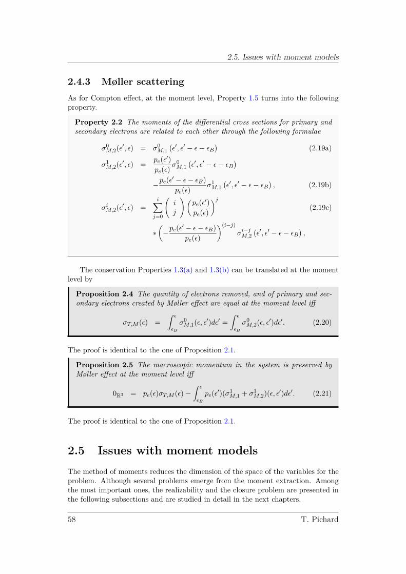
2.5. Issues with moment models
2.4.3 Møller scattering
As for Compton effect, at the moment level, Property 1.5 turns into the followingproperty.
Property 2.2 The moments of the differential cross sections for primary andsecondary electrons are related to each other through the following formulae
σ0M,2(ǫ′, ǫ) = σ0
M,1
(ǫ′, ǫ′ − ǫ− ǫB
)(2.19a)
σ1M,2(ǫ′, ǫ) =
pe(ǫ′)
pe(ǫ)σ0M,1
(ǫ′, ǫ′ − ǫ− ǫB
)
−pe(ǫ′ − ǫ− ǫB)
pe(ǫ)σ1M,1
(ǫ′, ǫ′ − ǫ− ǫB
), (2.19b)
σiM,2(ǫ′, ǫ) =i∑
j=0
(
ij
)(pe(ǫ
′)
pe(ǫ)
)j
(2.19c)
∗(
−pe(ǫ′ − ǫ− ǫB)
pe(ǫ)
)(i−j)
σi−jM,2
(ǫ′, ǫ′ − ǫ− ǫB
),
The conservation Properties 1.3(a) and 1.3(b) can be translated at the momentlevel by
Proposition 2.4 The quantity of electrons removed, and of primary and sec-ondary electrons created by Møller effect are equal at the moment level iff
σT,M (ǫ) =
∫ ǫ
ǫB
σ0M,1(ǫ, ǫ′)dǫ′ =
∫ ǫ
ǫB
σ0M,2(ǫ, ǫ′)dǫ′. (2.20)
The proof is identical to the one of Proposition 2.1.
Proposition 2.5 The macroscopic momentum in the system is preserved byMøller effect at the moment level iff
0R3 = pe(ǫ)σT,M (ǫ) −∫ ǫ
ǫB
pe(ǫ′)(σ1
M,1 + σ1M,2)(ǫ, ǫ′)dǫ′. (2.21)
The proof is identical to the one of Proposition 2.1.
2.5 Issues with moment models
The method of moments reduces the dimension of the space of the variables for theproblem. Although several problems emerge from the moment extraction. Amongthe most important ones, the realizability and the closure problem are presented inthe following subsections and are studied in detail in the next chapters.
58 T. Pichard

2. Moment models
2.5.1 Realizability property
In order to relate more closely the moment model to the associated kinetic model,one may want to reconstruct a fluence ψ(Ω) based on the solution ψ of a momentequation. At the kinetic level, a fluence ψ is necessarily non-negative because itcorresponds to a density of particles in a certain variable space (see Definition (1.9)).Then, based on Definitions 2.2(a) and 2.2(b) of the moments, physically relevantsolutions to moment equations such as (2.2) or (2.3) need to be the moments of anon-negative function ψ according to the Ω variable (or µ in 1D). This imposes acondition on the vector of moment afterward called realizability condition.
A vector ψ (or a set of tensors (ψ0, ψ1, ..., ψi)) is called realizable if there existsat least one non-negative distribution ψ(Ω) such that ψ is composed of momentsof ψ. This theoretical definition is complicated to use for practical applications.Therefore practical characterization of the realizability property are seeked. Thenext chapter is devoted to this problem.
2.5.2 Closure problem
The moment system (2.3) does not have a unique solution. This can easily beobserved because it has more unknowns (ψ0, ψ1, ..., ψN ) and ψN+1 (or ψ and F invectorial notation) than equations. Especially, the moments of the solution to thekinetic equation (1.11) are in the set of the solutions of the moment system (2.3).
In order to have a unique solution to the moment problem (2.3), one needs toclose the system. This closure consists in adding relations in order to have as manyunknowns as equations. Commonly, this closure consists in expressing ψN+1 as afunction of the other moments (ψ0, ..., ψN ). This problem is commonly solved byreconstructing an ansatz ψR having (ψ0, ..., ψN ) as moments of order 0 to N andthen the closure relation is chosen to be
ψN+1 =⟨
Ω⊗N+1ψR⟩
.
In order to relate the moment model to the underlying kinetic model, one maychose ψR to be non-negative, and therefore the closure problem is related to therealizability problem through the construction of this representing ansatz. Chapter4 is devoted to this problem.
2.5.3 Boundary conditions
The moment extraction procedure of Section 2.2 is well-understood in the interiorx ∈ int(Z). However, defining properly boundary conditions for moment modelscorresponding to the underlying kinetic ones remains an open problem.
The kinetic boundary conditions impose incoming fluxes (see Section 1.5), i.e.ψ is fixed to ψb only on Γ−. As moment extraction is an integration over the wholeunit sphere S2, this does not provide enough information to defined the whole fluxF on the boundary for moment equations.
According to the theory of hyperbolic equations (see e.g. [13, 4, 15]), not allthe flux F needs to be imposed on the boundary and one may define boundary
Mathematical modelling for dose deposition in photontherapy 59

2.5. Issues with moment models
conditions for moment equations based on this theory. However, it remains unclearhow to relate such boundary conditions to the underlying kinetic ones in the generalcase.
Several approaches are based on the study of the half space problem (see e.g.[19, 5]). This problem was also adressed e.g. [29, 37, 18] in the particular case oflinear closures (see the PN closures in Subsection 4.7.1 below). Other methods, suchas the partial moment method [38, 17], circumvent this issue.
The problem of boundary conditions for moment equations is not dealt with inthis manuscript. In Part III, boundary conditions for the moment equations areimposed at the discrete level. They are assumed to approximate the underlyingkinetic boundary conditions accurately enough for the present applications.
60 T. Pichard

Appendix
2.A Moments of the collision operators
Integrating the collision operators over the angular variable Ω is not trivial. Com-putations are summarized here. Only the 3D computations are shown, the 1D onescan be deduced from them.
2.A.1 Moments of a linear Boltzmann gain term
Generically, a kinetic linear Boltzmann gain term can be written
G(ψ)(Ω) =
∫
S2σ(Ω′.Ω)ψ(Ω′)dΩ′,
where the x and ǫ variables are removed because they can be seen as parameters inthis equation.
Moment tensors
By using the change of variable Ω” = RTΩ where the rotation R is such thatΩ′R = e1, the moments of order 0 and 1 of G(ψ) in tensorial notation reads
G0(ψ)(Ω) =
∫
S2
∫
S2σ(Ω′.Ω)ψ(Ω′)dΩ′dΩ
=
∫
S2
∫
S2σ(Ω′.Ω)dΩψ(Ω′)dΩ′ = σ0ψ0,
G1(ψ)(Ω) =
∫
S2
∫
S2Ωσ(Ω′.Ω)ψ(Ω′)dΩ′dΩ
=
∫
S2
∫
S2Ωσ(Ω′.Ω)dΩψ(Ω′)dΩ′
=
∫
S2R
∫
S2Ω”σ(Ω”e1)dΩ”ψ(Ω′)dΩ′
=
∫
S2Re1σ
1ψ(Ω′)dΩ′ =
∫
S2Ω′σ1ψ(Ω′)dΩ′ = σ1ψ1,
where
σi = 2π
∫ +1
−1µiσ(µ)dµ.
61

2.A. Moments of the collision operators
The computation of the moment of order two in tensorial form of this gain termis presented (corresponding to (2.5c)). Then the computation in vectorial form ispresented, and one can obtains the moment of any order i in tensorial form from it.
Multiplying G(ψ)(Ω) by Ω ⊗ Ω and integrating it over all Ω ∈ S2 yields
G2(ψ)(Ω) =
∫
S2Ω ⊗ Ω
∫
S2σ(Ω′.Ω)ψ(Ω′)dΩ′dΩ
=
∫
S2
∫
S2Ω ⊗ Ωσ(Ω′.Ω)dΩψ(Ω′)dΩ′.
By using the change of variable Ω” = RTΩ where a rotation R is such that Ω′R = e1,the moments of order 0 and 1 of G(ψ) in tensorial notation reads
∫
S2Ω ⊗ Ωσ(Ω′.Ω)dΩ =
∫
S2(RTΩ”) ⊗ (RTΩ”)σ(e1.Ω”)dΩ”
= RT∫
S2Ω” ⊗ Ω”σ(e1.Ω”)dΩ”R
= RT∫
S2
µ”2 µ”√
1 − µ”2c µ”√
1 − µ”2s
µ”√
1 − µ”2c (1 − µ”2)c2 (1 − µ”2)cs
µ”√
1 − µ”2s (1 − µ”2)cs (1 − µ”2)s2
σ(µ”)dΩ”R,
= 2πRT∫ +1
−1
µ”2 0 0
0 1−µ”2
2 0
0 0 1−µ”2
2
σ(µ”)dµ”R
= RT (σ0 − σ2
2Id+
3σ2 − σ0
2e1)R
=σ0 − σ2
2Id+
3σ2 − σ0
2Ω ⊗ Ω,
where c = cosφ” and s = sinφ”. This leads to (2.5c).
Moment vector
Multiplying G(ψ)(Ω) by a vector m(Ω) and integrating it over Ω ∈ S2 yields
G(ψ)(Ω) =
∫
S2m(Ω)
∫
S2σ(Ω′.Ω)ψ(Ω′)dΩ′dΩ
=
∫
S2
∫
S2m(Ω)σ(Ω′.Ω)dΩψ(Ω′)dΩ′
Now using the change of variable Ω” = RΩ leads to∫
S2m(Ω)σ(Ω′.Ω)dΩ =
∫
S2m(RTΩ”)σ(e1.Ω”)dΩ”.
Suppose m(Ω) is a linearily independent family generating the set of polynomials ofdegree N over the unit sphere S2, then the vector m(RTΩ”) can be written
m(RTΩ”) = A(Ω”)m(Ω′),
62 T. Pichard

2. Moment models
where the components of the matrix A(Ω”) are linear combinations of the compo-nents of m(Ω”). This matrix can be computed for particular choices of m(Ω), butthere is, a priori, no simple formula general to any degree N .
Therefore one obtains
G(ψ)(Ω) = sψ(Ω),
s =
∫
S2A(Ω”)σ(e1.Ω”)dΩ”.
The components of the moment of order i (in tensorial form) of a linear Boltz-mann gain term are the same as the one of a moment vector. One can obtain themoments of this gain term from those computations.
Example 2.4 For the moments according to m(Ω) = (1,Ω), the matrix s reads
s =
(
σ0 0TR3
0R3 σ1Id
)
.
For the moments according to
m(Ω) = (Ω1, Ω2, Ω3, Ω21, Ω2
2, Ω23, Ω1Ω2, Ω1Ω3, Ω2Ω3),
the matrix s reads
s =
σ1Id 0R3×3 0R3×3
0R3×3
σ0 − σ2
2MR3×3 +
3σ2 − σ0
2Id 0R3×3
0R3×3 0R3×3
3σ2 − σ0
2Id
,
where
MR3×3 =
1 1 11 1 11 1 1
.
2.A.2 Moments of a Fokker-Planck diffusion operator
Similarily the computation of the moments of the Fokker-Planck agular diffusionterm is shown for moments under vectorial form and in the tensorial form for mo-ments of order two.
The Fokker-Planck diffusion term reads
∆Ωψ(Ω) = ∂µ(
(1 − µ2)∂µψ(Ω))
+1
1 − µ2∂2φψ(Ω). (2.22)
Mathematical modelling for dose deposition in photontherapy 63

2.A. Moments of the collision operators
Moment vector
Multiplying (2.22) by m(Ω), integrating it over all Ω ∈ S2 and using an integrationby parts leads∫
S2m(Ω)∆Ωψ(Ω)dΩ =
∫
S2m(Ω)
[
∂µ(
(1 − µ2)∂µψ(Ω))
+1
1 − µ2∂2φψ(Ω)
]
dΩ
=
∫
S2
[
∂µ(
(1 − µ2)∂µm(Ω))
+1
1 − µ2∂2φm(Ω)
]
ψ(Ω)dΩ.
Suppose m(Ω) is a linearily independent family generating the set of polynomials ofdegree N over the unit sphere S2. By exhibiting the value of
∂µ(
(1 − µ2)∂µm(Ω))
+1
1 − µ2∂2φm(Ω),
one can easily show that this vector is only composed of linear combinations ofm(Ω). This leads to the matrix formulation
[
∂µ(
(1 − µ2)∂µm(Ω))
+1
1 − µ2∂2φm(Ω)
]
= MFPm(Ω),
where the matrix MFP can be computed for any choice of m(Ω), e.g. when m(Ω) =(1,Ω)
MFPm(Ω) =
(
0 0R3
0R3 −2Id
)
m(Ω),
and when m(Ω) = (Ω1, Ω2, Ω3, Ω21, Ω2
2, Ω23, Ω1Ω2, Ω1Ω3, Ω2Ω3)
MFPm(Ω) =
−2Id 0R3×3 0R3×3
0R3×3 2MR3×3 − 6Id 0R3×3
0R3×3 0R3×3 −6Id
m(Ω),
MR3×3 =
1 1 11 1 11 1 1
Again the moments under tensorial form can be deduced from this notation.
Moment tensor
In the special case N = 0 and N = 1, the moment of (2.22) under tensorial notationreads
∫
S2∆Ωψ(Ω)dΩ = 0,
∫
S2Ω∆Ωψ(Ω)dΩ =
∫
S2
[
∂µ(
(1 − µ2)∂µΩ)
+1
1 − µ2∂2φΩ
]
ψ(Ω)dΩ,
=
∫
S2−2Ωψ(Ω)dΩ,
= −2ψ1.
64 T. Pichard

2. Moment models
In the special case N = 2, the moment of (2.22) under tensorial notation reads∫
S2Ω ⊗ Ω∆Ωψ(Ω)dΩ =
∫
S2
[
∂µ(
(1 − µ2)∂µΩ ⊗ Ω)
+1
1 − µ2∂2φΩ ⊗ Ω
]
ψ(Ω)dΩ,
=
∫
S2(2Id− 6Ω ⊗ Ω)ψ(Ω)dΩ,
=
∫
S2(2tr(Ω ⊗ Ω)Id− 6Ω ⊗ Ω)ψ(Ω)dΩ,
= 2tr(ψ2)Id− 6ψ2.
Mathematical modelling for dose deposition in photontherapy 65

2.A. Moments of the collision operators
66 T. Pichard

Bibliography
[1] G. W. Alldredge, C. D. Hauck, D. P. O’Leary, and A. L. Tits. Adaptive changeof basis in entropy-based moment closures for linear kinetic equations. J. Com-put. Phys., 74(4), february 2014.
[2] G. W. Alldredge, C. D. Hauck, and A. L. Tits. High-order entropy-basedclosures for linear transport in slab geometry II: A computational study of theoptimization problem. SIAM J. Sci. Comput., 34(4):361–391, 2012.
[3] A. M. Anile and S. Pennisi. Thermodynamic derivation of the hydrodynamicalmodel for charge transport in semiconductors. Phys. Rev. B, 46:13186–13193,1992.
[4] C. Bardos, A. Y. Leroux, and J. C. Nedelec. First order quasilinear equationswith boundary conditions. Commun. Part. Diff. Eq., 4(9):1017–1034, 1979.
[5] A. Bensoussan, J.-L. Lions, and G. C. Papanicolaou. Boundary layers andhomogenization of transport processes. Publ. RIMS, Kyoto Univ., 15:53–157,1979.
[6] C. Berthon, P. Charrier, and B. Dubroca. An HLLC scheme to solve the M1
model of radiative transfer in two space dimensions. J. Sci. Comput., 31(3):347–389, 2007.
[7] Y. Bourgault, D. Broizat, and P.-E. Jabin. Convergence rate for the method ofmoments with linear closure relations. Kin. Rel. Mod., 8(1):1–27, 2015.
[8] C. Buet and B. Despres. Asymptotic preserving and positive schemes for radi-ation hydrodynamics. J. Comput. Phys., 215(2):717–740, July 2006.
[9] C. Canuto, M. Y. Hussaini, A. Quarteroni, and Th. A. Zang. Spectral methods:Fundamental in single domains. Springer, 2006.
[10] S. Chandrasekhar. On the radiative equilibrium of a stellar atmosphere. Astro-phys. J., 99:180 – 190, 1943.
[11] S. Chandrasekhar. On the radiative equilibrium of a stellar atmosphere X.Astrophys. J., 103:351 – 370, 1946.
67

BIBLIOGRAPHY
[12] S. Chandrasekhar. Radiative transfer. Dover publications, 1960.
[13] R. J. Diperna. Uniqueness of solutions to hyperbolic conservation laws. IndianaUniv. Math. J., 28(1):137–188, 1979.
[14] B. Dubroca and J.-L. Feugeas. Hiérarchie des modèles aux moments pour letransfert radiatif. C. R. Acad. Sci. Paris, 329:915–920, 1999.
[15] B. Dubroca and G. Gallice. Resultats d’existence et d’unicite du problème mixtepour des systems hyperboliques de lois de conservation monodimensionnels.Commun. Part. Diff. Eq., 15(1):59–80, 1990.
[16] R. Duclous. Modélisation et simulation numérique multi-échelle du transportcinétique électronique. PhD thesis, Université de Bordeaux 1, 2009.
[17] M. Frank. Partial moment models for radiative transfer. PhD thesis, TeschnicheUniversität Kaiserslautern, July 2005.
[18] B. D. Ganapol, C. T. Kelley, and G. C. Pomraning. Asymptotically exactboundary conditions for the PN equations. Nucl. Sci. Eng., 114, 1993.
[19] F. Golse, S. Jin, and C. D. Levermore. A domain decomposition analysis for atwo-scale linear transport problem. ESAIM-Math. Model. Num., 37(6):869–892,2003.
[20] H. Grad. On the kinetic theory of rarefied gases. Commun. Pur. Appl. Math.,2(4):331–407, 1949.
[21] C. Groth and J. McDonald. Towards physically realizable and hyperbolic mo-ment closures for kinetic theory. Cont. Mech. Therm., 21(6):467–493, 2009.
[22] S. Guisset, S. Brull, B. Dubroca, E. d’Humières, S. Karpov, and I. Potapenko.Asymptotic-preserving scheme for the M1-Maxwell system in the quasi-neutralregime. Commun. Comput. Phys., 19:301–328, 2016.
[23] S. Guisset, J.G. Moreau, R. Nuter, S. Brull, E. d’Humieres, B. Dubroca, andV.T. Tikhonchuk. Limits of the M1 and M2 angular moments models for kineticplasma physics studies. J. Phys. A: Math. Theor., 48, 2015.
[24] T. Hanawa and E. Audit. Reformulation of the M1 model of radiative transfer.J. Quant. Spectros. Radiat. Transfer, 145:9 – 16, 2014.
[25] C. Hauck. Entropy-based moment closures in semiconductor models. PhD the-sis, University of Maryland, 2006.
[26] C. Hauck and R. McClarren. Positive PN closures. SIAM J. Sci. Comput.,32(5):2603–2626, 2010.
[27] C. D. Hauck. High-order entropy-based closures for linear transport in slabgeometry. Commun. Math. Sci, 9(1):187–205, 2011.
68 T. Pichard

BIBLIOGRAPHY
[28] C. D. Hauck, C. D. Levermore, and A. L. Tits. Convex duality and entropy-based moment closures: Characterizing degenerate densities. SIAM J. ControlOptim., 47(4):1977–2015, 2008.
[29] E. W. Larsen and G. C. Pomraning. The PN theory as an asymptotic limitof transport theory in planar geometry I: Analysis. Nucl. Sci. Eng., 109(49),1991.
[30] C. D. Levermore. Relating Eddington factors to flux limiters. J. Quant. Spec-tros. Radiat. Transfer, 31:149–160, 1984.
[31] C. D. Levermore. Moment closure hierarchies for kinetic theories. J. Stat.Phys., 83(5–6):1021–1065, 1996.
[32] J. Mallet, S. Brull, and B. Dubroca. An entropic scheme for an angular momentmodel for the classical Fokker-Planck-Landau equation of electrons. Commun.Comput. Phys., 15(2):422–450, 2014.
[33] J. Mallet, S. Brull, and B. Dubroca. General moment system for plasma physicsbased on minimum entropy principle. Kin. rel. mod., 8(3):533–558, 2015.
[34] J. Mcdonald and M. Torrilhon. Affordable robust moment closures for CFDbased on the maximum-entropy hierarchy. J. Comput. Phys., 251:500–523,2013.
[35] G. C. Pomraning. The equations of radiation hydrodynamics. Pergamon Press,1973.
[36] S. La Rosa, G. Mascali, and V. Romano. Exact maximum entropy closure ofthe hydrodynamical model for Si semiconductors: The 8-moment case. SIAMJ. Appl. Math., 70(3):710–734, 2009.
[37] R. P. Rulko, E. W. Larsen, and G. C. Pomraning. The PN theory as an asymp-totic limit of transport theory in planar geometry II: Numerical results. Nucl.Sci. Eng., 109(76), 1991.
[38] R. Turpault, M. Frank, B. Dubroca, and A. Klar. Multigroup half space momentapproximations to the radiative heat transfer equations. J. Comput. Phys.,198(1):363 – 371, 2004.
Mathematical modelling for dose deposition in photontherapy 69

BIBLIOGRAPHY
70 T. Pichard

Chapter 3
Realizability
3.1 Introduction
In order to provide deeper physical meaning to the solution of moment equation,one aims to relate the solution ψ of moment equation such as (2.3) to an underlyingkinetic fluence ψ.
Among the properties that satisfy a kinetic fluence ψ, this chapter focuses on thepositivity. Indeed, since ψ is a density in the space Z × [ǫmin, ǫmax] × S2, a negativevalue of ψ is non-sense as it corresponds to a negative quantity of particles.
The necessity for a density to be positive is well understood. However it becomesmore complicated, after extraction of moments, to determine whether a vector ψis the moment vector of a non-negative function ψ. A vector is called realizableif it is the moment vector of a non-negative function ψ(Ω). The definition of therealizability property being difficult to use for practical applications, one typicallyseeks characterizations.
The study of the realizability property originally emerged in the end of thenineteenth century. This problem was mentioned by P. L. Chebyshev in 1873 ([8])and was pushed forward by A. Markov ([21, 22]). However, it is T.-J. Stieltjeswho gave the name "the Moment Problem" ([34]) to the problem of characterizingwhether a vector V is realizable. This field of study was widely developed (see e.g.with [1, 2, 17, 9, 19] and references therein) after E. Artin solved the 17-th Hilbertproblem ([3, 13])
Nowadays, the "moment problem" refers to the problem of characterizing therealizability of a vector V when the domain S of integration (for our purpose, S =[−1, 1] in 1D, and S = S2 in 3D) can be identified to a subset of R. Amongthe moment problems, the problems of Hamburger (S = R), Hausdorff (S = [a, b]),Stieltjes (S = R
+) and Toeplitz (S = S1) were solved and practical characterizationsare available (see e.g. Subsection 3.3.2 and [1, 9, 18]).
Commonly when the number of moments is finite, i.e. the vector ψ ∈ RN with
N < ∞, the problem is called "truncated moment problem". When the set of inte-gration S is not restricted to one dimension, such as in the present 3D problem, theproblem is called "the generalized moment problem". No practical characterizationof the realizability property were provided in the general case where the set of inte-gration S is not one dimensional and for arbitrarily large order N of moments. The
71

3.2. Preliminaries
moment problem on compact algebraic varieties (and semi-algebraic varieties), com-monly called K-moment problem is widely studied ([12, 10, 20, 4]), but only partialresults were obtained for moments on S2. Some of them are recalled in this chapterand will be used in the next one to study the realizability of moment closures.
3.2 Preliminaries
The truncated moment problem, i.e. the problem of characterizing whether a vectorV is a moment vector of a positive function ψ presents much more difficulties in 3Das 1D. Although similar methods are used for both problems. A generic workframeis given for both 1D and 3D problems. The generic variable of integration is writtenx and it belongs to a set S, i.e. when studying 1D problems
x = µ ∈ [−1, 1] = S
and for 3D problemsx = Ω ∈ S2 = S.
The set of polynomials of degree less or equal to K is denoted RK [X] in 1D, or
RK [X1, X2, X3] in 3D.
3.2.1 The realizability domain
For writing purposes, the definition of the realizability property given here is slightlydifferent compared to the one given in the introduction, i.e. the underlying functionψ is chosen to be strictly positive instead of non-negative. However, one can provethat those two problems are equivalent, e.g. with the work of [23, 5, 6, 7, 15, 31, 14].
The following notations and definitions are used
Notation 3.1 The set of strictly positive L1 functions over a set S is denotedL1(S)+, i.e. f ∈ L1(S)+ iff
f ∈ L1(S) and ess infS
f > 0.
The realizability property is commonly studied for moments under vectorial form(or under matricial form, see Subsection 3.2.2).
The truncated moment problem yields
Does there exist a function ψ ∈ L1(S)+, such that V = 〈mψ〉? (3.1)
Remark that in 1D or 3D, only moments on the compact sets [−1, 1] and S2 arestudied. Then having ψ ∈ L1(S) is sufficient for the existence of the moment ac-cording to any polynomial p. Indeed, on a compact S the polynomial p is boundedby min(p) ∈ R and max(p) ∈ R and so
min(p) 〈ψ〉 ≤ 〈pψ〉 ≤ max(p) 〈ψ〉 .Therefore 〈pψ〉 exists.
72 T. Pichard

3. Realizability
Definition 3.1 The realizability domain Rm associated to a vector of polyno-mials m over S is the set of all realizable moment vectors
Rm :=
〈mψ〉 , ψ ∈ L1(S)+
. (3.2)
We first prove the following proposition.
Proposition 3.1 If m is a linearily independent family of polynomials over S,then the realizability domain Rm is open.
Proof Suppose V = 〈mψ〉 ∈ Rm and define
ǫ := ess infS
ψ > 0.
Let us exhbibit a neighborhood of V included in Rm.Define
Vi = 〈mmi〉 .Simple computations show that the matrix 〈m ⊗ m〉 is symmetric positive defi-nite, and therefore non-singular. Therefore the family (Vi)i=1,...,Card(m) of itscolumn is a basis of RCard(m).
Therefore for all α > 0, the set
V =
V + α∑
i
λiVi, λi ∈] − 1, 1[, i = 1, ..., Card(m)
(3.3)
is a neighborhood of V in RCard(m).
Choose e.g.
α =ǫ
2Card(m)> 0.
With this choice of α, one can easily show that
α∑
i
λimi(x) > −ǫ, ∀x ∈ S, ∀λi ∈] − 1, 1[, i = 1, ..., Card(m).
Therefore, with this choice of α, each vector of the set (3.3) is representedby a function
ψ = ψ + α∑
i
λimi ∈ L1(S)
such that ess infS
ψ > ǫ − ǫ2 > 0. Therefore ψ ∈ L1(S)+ and each point of V
is included in Rm. For each point V ∈ Rm, there exists a neighborhood of Vincluded in Rm.
In order to study the geometry of the realizability domain, and especially itsboundary ∂Rm, one generally study at a slightly more general problem. By consid-ering that L1(S)+ is a subset of M(S), the set of the Borel measures on S, one cangeneralize the notion of moments.
Mathematical modelling for dose deposition in photontherapy 73

3.2. Preliminaries
Example 3.1 Suppose S = [−1, 1] and m(µ) = (1, µ). Consider the sequence(ψk)k∈N defined by
ψk(µ) =1
k√
2πexp
(
−(µ− 1√
2k
)2)
.
One can verify that ψk is bounded in L1(S) norm by 1. However the sequenceψk does not converge in L1(S), while the sequence of its moments
∫ +1
−1(1, µ)ψk(µ)dµ −→
k→∞(1, 1)
does converge in R2.
In the sense of measures, ψk converges to a Dirac measure in µ = 1
ψk(µ) −→k→∞
δ(µ− 1),
and therefore the sequence of moments converges to the moments according tothis measure
∫
m(µ)ψk(µ)dµ −→k→∞
∫ +1
−1m(µ)δ(µ− 1) = (1, 1).
This examples is a motivation to extend the notion of moments according to L1
functions to moments according to measures.Therefore one can generalize the truncated moment problem by looking for a
representing measure γ instead of a positive function ψ ∈ L1(S)+.
The truncated moment problem (according to measures) yields
Does there exist a measure γ such that V =
∫
Smdγ(x)? (3.4)
This notion of moments according to a measure is required in order to characterizethe boundary of the realizability domain Rm.
In the next sections, the following set is studied.
Definition 3.2 The set Rmm associated to a vector of polynomials m is defined
by
Rmm :=
V ∈ RCard(m), s.t. V = lim
k→∞〈mψk〉 (3.5)
for some bounded sequence ψk in L1(S)+
.
Remark that each vector of Rmm is represented by some measure γ
V ∈ Rmm ⇒ V =
∫
Sm(x)dγ(x).
According to Definition 3.2 and to Proposition 3.1, the following relations hold
74 T. Pichard

3. Realizability
Rmm = Rm ∩ R
Card(m), Rm = int(Rmm), (3.6)
where the superscript E refers to the closure of a set E and int(E) refers to theinterior of a set E.
Definition 3.1 of the realizability domain Rm (and the definition of the set Rmm) is
difficult to apply to practical problems. Instead, one typically aims to characterizethe realizability property by some numerical conditions easier to check. For thispurpose, the following definition is introduced.
Definition 3.3 A convex cone C is a set stable by positive combinations, i.e.iff
∀(V1,V2) ∈ C2 ∀(α1, α2) ∈ (R∗+)2, α1V1 + α2V2 ∈ C.
The following property offers a first characterization of realizability property.
Property 3.1 The realizability domain Rm and the set Rmm are convex cones.
Proof Using Definition 3.1 of the realizability property, there existsψ1 ∈ L1(S)+ and ψ2 ∈ L1(S)+ such that
V1 = 〈mψ1〉 , V2 = 〈mψ2〉 .
Therefore one obtains
α1V1 + α2V2 = 〈m (α1ψ1 + α2ψ2)〉 ,
where α1ψ1 + α2ψ2 ∈ L1(S)+.Similar computations hold for Rm
m.
Remark 3.1 This property is commonly used when constructing numerical schemesfor moment equations in order to prove that such schemes preserve the realiz-ability property from one step to another.
This characterization is convenient to construct realizable vector. However, inorder to exhibit the realizability property of a vector V, one still requires the knowl-edge of two realizable vectors V1 and V2, which is a priori not a simpler problemthan the original one (3.1).
Strategy: In order to find practical characterization of the realizability property,first a necessary condition for a vector to be realizable (Subsection 3.2.2) is seeked.Then, under this condition, the existence of a representing measure (Sections 3.3and 3.4) is proven by exhibiting one representing measure.
Mathematical modelling for dose deposition in photontherapy 75

3.2. Preliminaries
3.2.2 The Riesz functional
In the following, we seek necessary conditions for a vector to be realizable. Thoseare commonly easy to find. For numerical puprposes, we seek numerical inequalityconditions (because they are easy to check), i.e. we seek a set of N functions(fi)i=1,...,N such that
V ∈ Rm ⇒ ∀i = 1, ..., N, fi(V) > 0.
For notation purposes, the Riesz functional ([27, 19, 12]) is used. This operatorrearranges the terms of a vector V.
Definition 3.4 (Riesz functional)Consider a vector m ∈ (R[X])N of N polynomials of x, and a vector V ∈
RN .
The Riesz functional RV associated to V sends any polynomial p = λm onto
RV(p) = λV. (3.7)
Remark that the Riesz functional associated to V is a linear map from Span(m) toR.
If the vector V = 〈mψ〉 is the vector of moments of a function ψ ∈ L1(S)+, thenthe Riesz functional of p is the moment of ψ according to p
RV(p) = 〈pψ〉 .
In the next sections, the Riesz functional is also applied to matrices of polyno-mials. The Riesz functional is simply applied to each component of such a matrix
RV(M)i,j = RV(Mi,j).
Example 3.2 In 1D, consider the vector ψ = (ψ0, ψ1, ψ2) ∈ R3, and the
vector of monomials m(µ) = (1, µ, µ2). The Riesz function according to thevector ψ of the polynomial
p(µ) = 1 + 3µ− µ2
reads
Rψ(p) = Rψ(1) + 3Rψ(µ) − Rψ(µ2)
= ψ0 + 3ψ1 − ψ2 .
In 3D, consider the vector
ψ = (ψ0, ψ11, ψ
12, ψ
13, ψ
21,1, ψ
21,2, ψ
22,2, ψ
21,3, ψ
22,3, ψ
23,3) ∈ R
10,
and choose the vector of monomials m(Ω) = (1,Ω1,Ω2,Ω3). The Riesz func-
76 T. Pichard

3. Realizability
tional according to ψ of the matrix m ⊗ m reads
Rψ(m ⊗ m) = Rψ
1 Ω1 Ω2 Ω3
Ω1 Ω21 Ω1Ω2 Ω1Ω3
Ω2 Ω1Ω2 Ω22 Ω2Ω3
Ω3 Ω1Ω3 Ω2Ω3 Ω23
= Rψ
(
1 ΩT
Ω Ω ⊗ Ω
)
=
ψ0 ψ11 ψ1
2 ψ13
ψ11 ψ2
1,1 ψ21,2 ψ2
1,3
ψ12 ψ2
1,2 ψ22,2 ψ2
2,3
ψ13 ψ2
1,3 ψ22,3 ψ2
3,3
=
(
ψ0 (ψ1)T
(ψ1) ψ2
)
.
One can easily observe the following necessary condition.
Proposition 3.2 A vector V is realizable only if the Riesz functional preservespositivity, i.e.
V ∈ Rm ⇒(∀p ∈ Span(m), s.t. p > 0, then RV(p) > 0
). (3.8)
Proof Based on the definition of the realizability property
V ∈ Rm ⇒(∃ψ ∈ L1(S)+, s.t. V = 〈mψ〉
).
Suppose p = λm > 0 is a positive polynomial, then the product pψ > 0 ispositive and therefore the integral
RV(p) = 〈ψp〉 > 0.
In Sections 3.3 and 3.4, the condition (3.8) is studied when S = [−1, 1] and S = S2.
3.3 Moment realizability in 1D
This section is devoted to prove Theorems 3.1 and 3.2. This theorem was provene.g. in [16, 1, 9] in a slightly different way than presented here. The present proofis devoted to introduce the 3D problem of the next section and the basics of theatomic closure presented in [24, 30, 29] and recalled in Chapter 4 Section 4.7.2.
The vector of polynomials m(µ) is chosen to generate all the polynomials ofdegree less or equal to N . The vector of monomials of degree up to K is denoted
mK(µ) = (1, µ, ..., µK).
The vector mN is composed of linearily indepent polynomials generating RN [X].
For simplicity, the following choice of m is made
m = mN .
Mathematical modelling for dose deposition in photontherapy 77

3.3. Moment realizability in 1D
3.3.1 Positive polynomials on the interval [−1, 1]
This subsection is devoted to motivate the use of moment matrices.The condition (3.8) requires knowledge about the set of positive polynomials on
[−1, 1] as the condition RV(p) > 0 needs to be satisfied for all positive polynomialsp of degree less or equal to N .
First the following subset of positive polynomials of degree 2K on [−1, 1] isdefined.
Definition 3.5 A polynomial p ∈ R2K [X] of degree 2K is a sum of squares if
it has the form
p =J∑
i=1
p2i , for some J ∈ N and some (pi)i=1,...,J ∈ (RK [X])J .
The set of sum of squares of polynomials of degree K is denoted Σ2K [X].
Remark that a square of a polynomial q = λm for some λ ∈ RCard(m) can be
written
q2 = (λm)2 = λT (m ⊗ m)λ.
Example 3.3 Choose m(µ) = (1, µ). The polynomial
p(µ) = 6 + 6µ+ 2µ2
is a sum of squares, because it can be written e.g.
p(µ) = (1 + µ)2 + 12 + (2 + µ)2 =3∑
i=1
λTi (m(µ) ⊗ m(µ))λi,
where the coefficients λi read
λ1 = (1, 1), λ2 = (1, 0), λ3 = (2, 1).
Obviously sums of squares are non-negative, and the following characterizationsare a motivation to study moment matrices RV(m ⊗ m).
Proposition 3.3 ([26, 28]) Even case:All polynomials p ∈ R
2K [X] of degree 2K, strictly positive on [−1, 1] havethe form
p(µ) = p1(µ) + (1 − µ2)p2(µ), (3.9)
where p1 ∈ Σ2K [X] and p2 ∈ Σ2K−2[X] are sums of squares.
78 T. Pichard

3. Realizability
Proposition 3.4 ([26, 28]) Odd case:All polynomials p ∈ R
2K+1[X] of degree 2K + 1, strictly positive on [−1, 1]have the form
p(µ) = (1 − µ)p1(µ) + (1 + µ)p2(µ), (3.10)
where p1 ∈ Σ2K [X] and p2 ∈ Σ2K [X] are sums of squares.
The even and odd cases are subcases of both Putinar [26] and Schmüdgen [28]Positivstellensätze for univariate polynomials.
Propositions 3.3 and 3.4 can be rewritten under matricial form.
Even case:A polynomial p ∈ R
2K [X] is strictly positive on [−1, 1] iff there exists coefficients(λ1,i)i=1,...,J ∈ R
K×J and (λ2,i)i=1,...,J ∈ RK−1×J such that
p =J∑
i=1
[
λ1,iT (mK ⊗ mK)λ1,i + λ2,i
T(
(1 − µ2)mK−1 ⊗ mK−1
)
λ2,i
]
.
Odd case:A polynomial p ∈ R
2K+1[X] is strictly positive on [−1, 1] iff there exists coeffi-cients(λ1,i)i=1,...,J ∈ R
K×J and (λ2,i)i=1,...,J ∈ RK×J such that
p =J∑
i=1
[
λ1,iT ((1 − µ)mK ⊗ mK)λ1,i + λ2,i
T ((1 + µ)mK ⊗ mK)λ2,i
]
.
Using Proposition 3.2, this leads to writing the following necessary conditionsfor a vector to be realizable.
Even case:A vector V ∈ Rm2K
is realizable only if
RV (mK ⊗ mK) > 0, RV
(
(1 − µ2)mK−1 ⊗ mK−1
)
> 0.
Odd case:A vector V ∈ Rm2K+1 is realizable only if
RV ((1 − µ)mK ⊗ mK) > 0, RV ((1 + µ)mK ⊗ mK) > 0.
In the next subsections, those conditions are shown to be sufficient for V to berealizable.
3.3.2 The truncated Hausdorff moment problem
The aim of this subsection is to exhibit the solution of the truncated Hausdorf mo-ment problem in theorem 3.1 and 3.2, i.e. to give a necessary and sufficient condition
Mathematical modelling for dose deposition in photontherapy 79

3.3. Moment realizability in 1D
on matrices to be realizable moment matrices. This results was proven e.g. in [9].A proof of this theorem is provided in order to exhibit the particular representingmeasure (3.30) to realizable vector. This proof provides some understanding on po-tential representing measures for a moment vector V, especially when V ∈ Rm
m is onthe boundary of the realizability domain. Some of the ideas presented in this sectionwill be generalized for the multi-D problem and will be used in the next chapter toconstruct a realizable closure. Furthermore, the representing measure exhibited inthis subsection can be used to construct an atomic based closure which differs fromthe Kershaw closure as described in [16, 24, 30, 29].
The principle of the method consists in exhibiting a measure representing anyvector V satisfying particular constraints. This measure is decomposed into a regularpart, i.e the Lesbesgues measure multiplied by a positive scalar, and a discretemeasure, i.e. a sum of Dirac measures. One also observes that the regular partvanishes on the boundary of the realizability domain and vectors on the boundaryof the realizability domain can only be represented by a unique measure which is asum of Dirac measures.
First the following lemmas characterize potential singularities of the momentmatrices.
Lemma 3.1 (Even case) Suppose V ∈ R2K such that
RV (mK ⊗ mK) ≥ 0, (3.13a)
RV
(
(1 − µ2)mK−1 ⊗ mK−1
)
≥ 0, (3.13b)
and at least one of those matrices is singular.Even case 1: In the case when
rank (RV (mK ⊗ mK)) ≤ rank(
RV
(
(1 − µ2)mK−1 ⊗ mK−1
))
, (3.14)
there exists a polynomial p ∈ RJ [X] of degree J ≤ K with distinct real roots
included in ] − 1, 1[, such that
RV(p2) = 0. (3.15)
Even case 2: In the case when
rank (RV (mK ⊗ mK)) > rank(
RV
(
(1 − µ2)mK−1 ⊗ mK−1
))
, (3.16)
there exists a polynomial p ∈ RJ [X] of degree J ≤ K− 1 with distinct real roots
included in ] − 1, 1[, such that
RV((1 − µ2)p2) = 0. (3.17)
80 T. Pichard

3. Realizability
Lemma 3.2 (Odd case) Suppose V ∈ R2K+1 such that
RV ((1 + µ)mK ⊗ mK) ≥ 0, (3.18a)
RV ((1 − µ)mK ⊗ mK) ≥ 0, (3.18b)
and at least one of those matrices is singular.Odd case 1: In the case when
rank (RV ((1 + µ)mK ⊗ mK)) ≥ rank (RV ((1 − µ)mK ⊗ mK)) , (3.19)
there exists a polynomial p ∈ RJ [X] of degree J ≤ K with distinct real roots
included in ] − 1, 1[, such that
RV((1 − µ)p2) = 0. (3.20)
Odd case 2: In the case when
rank (RV ((1 + µ)mK ⊗ mK)) ≤ rank (RV ((1 − µ)mK ⊗ mK)) , (3.21)
there exists a polynomial p ∈ RJ [X] of degree J ≤ K with distinct real roots
included in ] − 1, 1[, such that
RV((1 + µ)p2) = 0. (3.22)
Proof For the sake of brevity, the proof is written for the Even case 1. Theresult in the other cases can be obtained by similar computations.
According to the hypothesis of the lemma and to (3.14), the matrix (3.13a)is singular. Then there exists λ ∈ R
K\0RK such that
λTRV (mK ⊗ mK)λ = RV
(
(λmK)2)
= 0. (3.23)
Define the polynomial p = λmK ∈ RK [X]. If several λ ∈ R
K satisfy (3.23), wechoose the one that provides a polynomial p = λmK of lowest degree. In thefollowing p is proven to have real distinct roots in [−1, 1].
p is real rooted: By contradiction, suppose p has a pair of complex roots,i.e. it has the form
p = (µ2 + 2bµ+ c2)q with q ∈ RK−2[X], (b, c) ∈ R
2 s.t. b2 < c.
Computing the Riesz functional of p2 reads
0 = RV
(
(µ2 + 2bµ+ c)2q2)
= RV
([
(µ+ b)2 +(
c− b2)]2
q2)
= RV
(
(µ+ b)4 q2)
+ κ1RV
(
(µ+ b)2 q2)
+ κ2RV
(
q2)
, (3.24)
κ1 = 2(
c− b2)
> 0, κ2 =(
c− b2)2> 0.
Mathematical modelling for dose deposition in photontherapy 81

3.3. Moment realizability in 1D
Remark that each polynomial (µ + b)4q2, (µ + b)2q2 and q2 is the square ofa polynomial. Thus, according to (3.13a) each term in (3.24) is non-negative.Since their sum is zero, each term is zero. In particular RV
(q2)
= 0 whichviolates the hypothesis that p is the polynomial of lowest degree satisfying (3.23).
p has distinct roots: By contradiction, suppose that one of the roots of pis a double root, i.e. p has the form
p = λmK = (µ− µ1)2q ∈ RJ [X].
The matrix RV(mK⊗mK) is real symmetric positive semi-definite and thereforediagonalizable. If λ ∈ R
K is such that
λTRV(mK ⊗ mK)λ = 0,
then one actually has
RV(mK ⊗ mK)λ = 0RK . (3.25)
Multiplying (3.25) by the vector λ2 ∈ RK such that λ2mK = q leads to write
that
RV ((mKλ2)(mKλ)) = RV
(
q2(µ− µ1)2)
= 0.
Therefore the polynomial p2 = q(µ − µ1) satisfy (3.23) which violates the hy-pothesis that p is the polynomial of lowest degree satisfying (3.23)
The roots of p are included in [−1, 1]: By contradiction, suppose thatone of the root µ1 of p is bigger than 1, i.e. p has the form
(µ− µ1)q
with q ∈ RK−1[X] and µ1 ∈] + 1,+∞[. Computing the Riesz functional of p2
reads
RV
(
(µ− µ1)2q2)
= κ1RV
(
q2)
+ κ2RV
(
(1 − µ2)q2)
+κ3RV
(
(1 − µ)2q2)
+ κ4RV
(
(1 + µ)2q2)
,
κ1 = (1 − µ1)2 > 0, κ2 = |1 − µ1| > 0,
κ3 =|µ1| + µ1
2≥ 0, κ4 =
|µ1| − µ1
2≥ 0,
which leads again to RV
(q2)
= 0 and violates the hypothesis that p is thepolynomial of lowest degree satisfying (3.23).
Under the hypothesis of Lemmas 3.1 and 3.2, one can prove the existence of arepresenting measure for V.
82 T. Pichard

3. Realizability
Lemma 3.3 (Even case) If V ∈ R2K satisfies
RV(mK ⊗ mK) ≥ 0, RV
(
(1 − µ2)mK−1 ⊗ mK−1
)
≥ 0,
and such that one of those matrices is singular, then there exists a representingmeasure for V.
Lemma 3.4 (Odd case) If V ∈ R2K+1 satisfies
RV ((1 − µ)mK ⊗ mK) ≥ 0, RV ((1 + µ)mK ⊗ mK) ≥ 0,
and such that one of those matrices is singular, then there exists a representingmeasure for V.
Proof The proof is again written for the even case when
rank (RV(mK ⊗ mK)) ≤ rank(
RV
(
(1 − µ2)mK−1 ⊗ mK−1
))
,
and the other cases can be obtained by reproducing those computations.Lemma 3.1 provides the existence of a polynomial p ∈ R
J [X] of degreeJ ≤ K having J distinct roots (µi)i=1,...,J in the interval [−1, 1] such thatRV(p2) = 0. Among the possible p, we choose one of lowest degree.
Suppose there exists a measure γ which moments are V, then
∫ +1
−1p2(µ)dγ(µ) = 0.
Since p2 is non-negative, if such a measure γ exists, its support Supp(γ), i.e. theintersection of all closed set the measure of which complements is zero, needsto be included in the set Z(p) of zeros of p
Supp(γ) ⊂ Z(p). (3.26)
The only measures having a union of a finite number of singletons µi forsupport have the form
γ =J∑
i=1
αiδ(µ− µi). (3.27)
Therefore, the rest of the proof consists in proving that there exists a uniqueset of coefficients αi > 0 such that the measure (3.26) has V for moments.
The moments according to γ of the form (3.27) read
∫ +1
−1mK(µ) ⊗ mK(µ)dγ(µ) =
J∑
i=1
αimK(µi) ⊗ mK(µi).
Mathematical modelling for dose deposition in photontherapy 83

3.3. Moment realizability in 1D
Then γ is a representing measure for V if non-negative scalars αi can be foundsuch that
RV(mK ⊗ mK) =J∑
i=1
αimK(µi) ⊗ mK(µi).
Write VJ the truncation of the vector V up to the J-th component. Byrearranging the terms composing the matrices mK(µi) ⊗ mK(µi) into vectorand removing the redundant terms, one can rewrite this problem
Mα = VJ ,
where M is a Vandermonde matrix, i.e. Mi,j = µj−1i and α ∈ R
J is the desiredvector of scalars. Vandermonde matrices are known to be invertible as long asthe µi are distinct which is verified here according to Lemma 3.1. It remains toverify that the coefficients αi ≥ 0 are positive.
Let us define the Lagrange polynomials
qi(µ) =J∏
j=1j 6=i
(µ− µj),
then computing the moment of γ according to q2i reads
RV(q2i ) = αiqi(µi)
2,
which is strictly positive according to the hypothesis that p is the polynomialof lowest degree such that RV(p2) = 0. Since the zeros of p are distinct, qi(µi)2
are strictly positive. Therefore the coefficients αi > 0, which leads to the result.
This proof provides several information on the representing measure on the boundaryof the realizability domain.
Definition 3.6 Suppose V ∈ Rmm is represented by a measure
γ =∑
i
αiδ(µ− µi)
composed only of Dirac measures. Then γ is called atomic representing measurefor V. Each Dirac measure δ(µ− µi) is called an atom.
A atomic representing measure composed of r atoms is called r-atomic rep-resenting measure.
Remark 3.2 The proof of Lemma 3.3 and 3.4 provides the uniqueness of therepresenting measure, which is atomic, under the hypothesis of Lemmas 3.3 and
84 T. Pichard

3. Realizability
3.4 which can be interpreted as requiring that V ∈ ∂Rmm is on the boundary of
the realizability domain.
With those lemmas, one obtains the following characterization of Rmm in 1D.
Theorem 3.1 (Truncated Hausdorff moment problem [1, 9]) Evencase:Consider V ∈ R
2K . The vector V ∈ Rmm2K
iff
RV(mK ⊗ mK) ≥ 0, RV
(
(1 − µ2)mK−1 ⊗ mK−1
)
≥ 0. (3.28)
Theorem 3.2 (Truncated Hausdorff moment problem [1, 9]) Oddcase:Consider V ∈ R
2K+1. The vector V ∈ Rmm2K+1
iff
RV ((1 − µ)mK ⊗ mK) ≥ 0, RV ((1 + µ)mK ⊗ mK) ≥ 0. (3.29)
Proof Necessary condition: Using Propositions 3.2 and 3.3, if V ∈ Rmm then
(3.28) and (3.29) are satisfied.Sufficient condition: The sufficiency part is proven by exhibiting one pos-
sible representing measure, i.e. a positive constant multiplied by the Lesbeguesmeasure plus a sum of Dirac measures.
The proof is again given for the even case. The result for the odd case canbe obtained by adapting the computations.
If one of the matrices (3.28) is singular, the existence of a representingmeasure is given by Lemma 3.3.
Suppose that the matrices (3.28) are non-singular, they are therefore strictlypositive according to the hypothesis.
Define V0 the moments according to the Lebesgues measure
V0 =
∫ +1
−1m(µ)dµ,
and define the functions
W(x) = V0 − xV,
M1(x) = RW(x)(mK ⊗ mK)
= RV0(mK ⊗ mK) − xRV(mK ⊗ mK),
M2(x) = RW(x)
(
(1 − µ2)mK−1 ⊗ mK−1
)
= RV0
(
(1 − µ2)mK−1 ⊗ mK−1
)
− xRV0
(
(1 − µ2)mK−1 ⊗ mK−1
)
.
Remark that M1 and M2 are matrices of linear functions of x ∈ R, in particulartheir components are C∞ functions of x. Furthermore, based on the hypothesis
Mathematical modelling for dose deposition in photontherapy 85

3.3. Moment realizability in 1D
and on the definition of V0, they satisfy
det(M1(0)) > 0, limx→+∞
det(M1(x)) < 0,
det(M2(0)) > 0, limx→+∞
det(M2(x)) < 0.
Using the intermediate value theorem, there exists positive scalars x > 0 suchthat det(M1(x)) = 0 and/or det(M2(x)) = 0. Write y the minimum of thosevalues. At that point, one has
M1(y) ≥ 0, M2(y) ≥ 0,
and one of those matrices is singular. According to Lemma 3.3, there exists aunique representing measure γ for W (y) which has the form
dγ(µ) =∑
i
αiδ(µ− µi),
where the scalars µi are the zeros of the characteristic polynomial of M1(y) orM2(y) (the one of minimal dimension or M1(y) if they have the same dimension)and the coefficients αi are the unique (positive) scalars such that this measurehas W (y) for moments.
Finally one verifies that the following measure
dγ(µ) + ydµ (3.30)
is positive and has V for moments.
The idea of this atomic decomposition follows from the form of the unique rep-resenting measure on the boundary ∂Rm
m and from the work of R. Curto and L.Fialkow ([9, 11, 12, 10]). This representing measure could be used to constructclosure of 1D moment equations.
3.3.3 The realizability condition in 1D
The existence of a representing measure γ for a vector V ∈ int(Rmm) in the interior
implies the existence of a positive L1([−1, 1])+ representing function ψ according(3.6). This leads to
Corollary 3.1 Even case:Consider V ∈ R
2K . The vector V ∈ Rm2Kis realizable iff
RV(mN ⊗ mN ) > 0, RV
(
(1 − µ2)mN−1 ⊗ mN−1
)
> 0. (3.31)
Corollary 3.2 Odd case:
86 T. Pichard

3. Realizability
Consider V ∈ R2K+1. The vector V ∈ Rm2K+1 is realizable iff
RV ((1 − µ)mN ⊗ mN ) > 0, RV ((1 + µ)mN ⊗ mN ) > 0. (3.32)
The next chapter is devoted to the closure problem. Commonly one aims todefine a closure ψN+1 such that the vector (ψ0, ..., ψN , ψN+1) ∈ RmN+1 is realizable.Corollaries 3.1 and 3.2 leads to the following requirements.
Corollary 3.3 ([16, 1]) Even case:Consider the vector V = (ψ0, ..., ψ2K−1, ψ2K) ∈ R
2K and write
V := (ψ0, ..., ψ2K−1, 0)
the vector V with the last component replaced by 0.The vector V ∈ Rm2K+2 is realizable iff
1. The truncated vector (ψ0, ..., ψ2K−1) ∈ Rm2K−1 is realizable
2. The last component ψ2K is bounded by
−det(
RV
(mK ⊗ mK
) )
det(
RV
(mK−1 ⊗ mK−1
) ) ≤ ψ2K , (3.33a)
ψ2K−2 +det
(RV
((1 − µ2)mK−1 ⊗ mK−1
) )
det(
RV
((1 − µ2)mK−2 ⊗ mK−2
) ) ≥ ψ2K . (3.33b)
Corollary 3.4 ([16, 1]) Odd case:Consider the vector V := (ψ0, ..., ψ2K , ψ2K+1) ∈ R
2K+1 and write
V := (ψ0, ..., ψ2K , 0)
the vector V with the last component replaced by 0.The vector V ∈ Rm2K+1 is realizable iff
1. The truncated vector (ψ0, ..., ψ2K) ∈ Rm2Kis realizable
2. The last component ψ2K+1 is bounded by
−ψ2K−det(
RV
((1 + µ) mK ⊗ mK
) )
det(
RV
((1 + µ)mK−1 ⊗ mK−1
) ) ≤ ψ2K+1, (3.34a)
ψ2K+det
(RV
((1 − µ) mK ⊗ mK
) )
det(
RV
((1 − µ)mK−1 ⊗ mK−1
) ) ≥ ψ2K+1. (3.34b)
The conditions (3.33a-3.33b) and (3.34a-3.34b) for the moment of order up to3 have the following form ([16, 24]). By extension, one also observes the following
Mathematical modelling for dose deposition in photontherapy 87

3.4. Moment realizability in 3D
condition for scalars to be a moment of order 0 of a positive function.
N=0: 0 < ψ0, (3.35a)
N=1: − ψ0 < ψ1 < ψ0, (3.35b)
N=2:|ψ1|2ψ0
< ψ2 < ψ0, (3.35c)
N=3: −ψ2+(ψ1 + ψ2)2
ψ0 + ψ1< ψ3 < ψ2 −(ψ1 − ψ2)2
ψ0 − ψ1. (3.35d)
Finally the realizability domain for the first order moments in 1D is characterizedby
R(1,µ) =(ψ0, ψ1) ∈ R
2, s.t. |ψ1| < ψ0, (3.36a)
R(1,µ,µ2) =(ψ0, ψ1, ψ2) ∈ R
3, s.t. |ψ1| < ψ0,|ψ1|2ψ0
< ψ2 < ψ0.
(3.36b)
The convex cones (3.36a) and (3.36b) are represented on Fig. 3.1 and 3.2. The firstset is represented in the plan (ψ0, ψ1) ∈ R
2, the second is represented in the plan(ψ1
ψ0 ,ψ2
ψ0
)
∈ R2.
ψ0
ψ1
R(1,µ)
Figure 3.1: Realizability domainR(1,µ) for moments of order up to 1in the space (ψ0, ψ1) ∈ R
2.
ψ2
ψ0
ψ1
ψ0
R(1,µ,µ2)
1
1-1
Figure 3.2: Realizability domainR(1,µ,µ2) for moments of order up to
2 in the space (ψ1
ψ0 ,ψ2
ψ0 ) ∈ R2.
3.4 Moment realizability in 3D
This section is devoted to introduce results about the realizability domain in 3Dwhich are used in the next chapter. Here the truncated moment problem on theunit sphere S2 is focused on.
88 T. Pichard

3. Realizability
3.4.1 Polynomials on S2
Before studying the truncated moment problem, one needs to choose a set of poly-nomials m defined on S2. Choosing S2 as the set of integration (and as the set ofdefinition of the polynomials) leads to the following major differences compared tothe 1D case:
1. Choosing Ω ∈ S2 ⊂ R3 forces us to study multivariate polynomials m(Ω).
Such multivariate polynomials can not be factorized as a product of polyno-mials of degree one or two.
2. The set of integration S2 is a compact algebraic variety defined by
S2 =
Ω ∈ R3, s.t. 1 − (Ω2
1 + Ω22 + Ω2
3) = 0
⊂ R3.
Similarily to the 1D case, one typically aim to choose the vector of polynomialsm such that it is composed of linearily independent polynomials and it generates allthe polynomials of degree less or equal to N . Although, the meaning of "indepen-dent" and of "generating" is ambiguous for multivariate polynomials on S2. For thispurpose, the following set is defined.
Definition 3.7 Define the polynomial
p0(X1, X2, X3) := 1 − (X21 +X2
2 +X23 ),
which is zero on S2.The set IN is the set of polynomials of degree N generated by p0
IN := p0RN−2[X1, X2, X3] =
p p0, p ∈ RN−2[X1, X2, X3]
. (3.37)
First the following proposition provides an additional constraint on vectors to berealizable.
Proposition 3.5 Consider a vector V ∈ Rmm, then
RV(IN ) = 0.
Proof Consider V ∈ Rm, then V is composed of moments of a function ψ ∈L1(S2)+. All the polynomials of p ∈ IN are zero on S2. Therefore the integralof their product ∫
S2p(Ω)ψ(Ω)dΩ = 0
is zero. By continuity, it also holds on the boundary of the realizability domain.
This result is illustrated through the following example that will be used in the nextchapter.
Mathematical modelling for dose deposition in photontherapy 89

3.4. Moment realizability in 3D
Example 3.4 Consider a vector V ∈ Rmm, then
RV
(
1 − (Ω21 + Ω2
2 + Ω23))
= 0. (3.38)
Writeψ0 = RV(1), ψ2 = RV(Ω ⊗ Ω).
Equation (3.38) provides the following relation between ψ0 and ψ2
ψ0 −(
ψ21,1 + ψ2
2,2 + ψ23,3))
= ψ0 − tr(ψ2) = 0.
The vector m is chosen to be linearily independent in the sense
Span(m) ∩ IN = 0, (3.39a)
and such that it generates RN [X1, X2, X3] in the following sense
Span(m) ∪ IN = RN [X1, X2, X3]. (3.39b)
i.e. m is a linearily independent and generating family modulo IN .The vector mK is defined to be composed of all monomials of degree K is written
mK =(
ΩK1 , ΩK−1
1 Ω2, ΩK−11 Ω3, ΩK−2
1 Ω22, ... ,ΩK
3
)
,
and the vector of all monomials of degree K − 1 and K is written
mK = (mK−1, mK).
The following choice of m is made
m = mN .
Example 3.5 For the first orders N = 1 and N = 2, one has
m1(Ω) = (1, Ω1, Ω2, Ω3) ,
m2(Ω) =(
Ω1, Ω2, Ω3, Ω21, Ω1Ω2, Ω2
2, Ω1Ω3, Ω2Ω3, Ω23
)
.
No polynomial of Span(m) can be factorized by p0, therefore this choice of msatisfy (3.39a). One shows that (3.39b) is satisfied by comparing the dimensions ofSpan(m), IN and R
N [X1, X2, X3].
Notation 3.2 After computations, the number of components of the vector mN
is (N + 1)2. It is afterward written
cN := Card(mN ) = (N + 1)2.
90 T. Pichard

3. Realizability
For the problem of moments on S2, positive polynomials are also used. Propositions3.3 and 3.4 can be generalized into Putinar ([26]) or Schmüdgen ([28]) (see alsoStengle [33]) Positivstellensätze in order to write a positive polynomial p on S2 as asum of squares
0 < p on S2 ⇔ p =∑
i
q2i . (3.40)
Although for multivariate polynomials, the degree of such a sum of squares repre-sentation is not bounded by the degree of p, i.e. in (3.40) a priori 2deg(qi) ≤ deg(p)does not hold ([32, 25]).
Sum of squares are still positive on S2, but there might be some positive poly-nomials of degree 2K which are not sum of squares of polynomials of degree K.Remark that Proposition 3.3 was not used in Subsection 3.3.2 and 3.3.3 but onlymotivated the use of moment matrices.
3.4.2 Realizability of first orders moments
Some explicit conditions were found for moments on the unit sphere of order up toone and to two. They recalled here because they will be used in the next chapter.
Realizability condition for moments of order up to one
The realizability condition for moments of order up to one on the unit sphere ischaracterized by the following proposition.
Proposition 3.6 ([16]) Consider the vector V ∈ Rc1 and write
ψ0 = RV(1), ψ1 = RV(Ω).
The vector V ∈ Rmm1
iff
|ψ1| ≤ ψ0. (3.41)
Furthermore, in the equality case, there exists a unique representing measure,which has the form
γ(Ω) = ψ0δ
(
Ω − ψ1
ψ0
)
,
One can easily see that the condition (3.41) is necessary for V to be in Rmm1
. Thiscondition was also proven to be sufficient in [16] by exhibiting the existence of thefollowing positive representing measure for V
γ(Ω) =(
ψ0 + |ψ1|)
δ
(
Ω − ψ1
|ψ1|
)
+(
ψ0 − |ψ1|)
δ
(
Ω +ψ1
|ψ1|
)
.
Here γ is a positive measure as long as (3.41) is satisfied.
Mathematical modelling for dose deposition in photontherapy 91

3.4. Moment realizability in 3D
This result leads to the following characterization of the realizability domainRm1
Rm1 =
(ψ0, ψ1) ∈ R × R3, s.t. |ψ1| < ψ0
. (3.42)
This condition can be interpreted at the physical level by the boundedness of thefluxes. Remark the similarilty with the 1D condition (3.35b).
Realizability condition for moments of order up to two
The realizability condition for moments of order up to two on the unit sphere ischaracterized by the following proposition.
Proposition 3.7 ([16]) Consider the vector V ∈ Rc2 and write
ψ1 = RV(Ω), ψ2 = RV(Ω ⊗ Ω).
The vector V ∈ Rmm2
iff
ψ0 := tr(ψ2) ≥ 0, (3.43a)
ψ0ψ2 − ψ1 ⊗ ψ1 ≥ 0. (3.43b)
Furthermore, if one of the eigenvalues of (3.43b) is zero, i.e.
∃W ∈ R3, s.t. W
(
ψ0ψ2 − ψ1 ⊗ ψ1)
W = 0,
then the support of any representing measure γ for V is in the set of zeros ofthe polynomial p := (Ω − ψ1)W , i.e.
Supp(γ) ⊂ Z(p). (3.44)
One verifies that the condition (3.43) is necessary for V to be in Rmm2
. This conditionwas also proven to be sufficient in [16] by exhibiting the existence of one representingmeasure for V positive as long as V satisfies (3.43).
This result leads to the following characterization of the realizability domainRm2
Rm2 =
V ∈ Rc2 , s.t. ψ0ψ2 − ψ1 ⊗ ψ1 > 0
. (3.45)
Remark the similarilty with the 1D condition (3.35c).
3.4.3 Partial results for higher order moments
No practical characterization of the realizability condition for high order moments onthe unit sphere S2 is known. This subsection is devoted to (partially) complete thedescription of the realizability domain in multi-D and to provide few more results.Those results do not provide a practical characterization of the realizability propertyin the general case but they provide .
92 T. Pichard
3. Realizability
The necessary conditions for a vector V to be realizable proposed in (3.8) canbe completed.
For instance, one can first remark that any realizable vector V ∈ Rmm2K
verifiesthe following conditions.
Proposition 3.8 If V ∈ Rmm2K
then
RV(I2K) = 0, RV(mK ⊗ mK) ≥ 0.
Suppose furthermore that there exists a polynomial 0 ≤ p ∈ R2K [X1, X2, X3]
non-negative over S2 such that
RV(p) = 0.
Then the support of γ is included in the zero set of p
Supp(γ) ⊂ Z(p).
Proof If V ∈ Rmm2K
then it has a positive representing measure γ, i.e.
V =
∫
S2m2K(Ω)dγ(Ω).
Based on the definition of the Riesz functional, for a non-negative polynomialp ∈ R
2K [X1, X2, X3]
RV(p) =
∫
S2p(Ω)dγ(Ω) = 0
implies that Supp(γ) ⊂ Z(p).The equality RV(I2K) = 0 is provided by Proposition 3.5. Any square
of a polynomial is non-negative, and γ is a positive measure. This leads to theinequality.
A 1D version of this result was also used in the proof of Lemmas 3.3 and 3.4.One method to characterize the realizability for arbitrary high order moments
over S2 consists in exhibiting a representing measure having the form of a sumof Dirac measures. The following method aims to exhibit an atomic representingmeasure for a vector V2K ∈ R
c2K composed of 2K + 2 atoms instead of 2K and,contrarily to the method used to exhibit the measure (3.30) in 1D, this representingmeasure is composed only of atoms and has no regular part dΩ. For this purpose,the following notations are introduced.
Definition 3.8 Consider V2K ∈ Rc2K and write
MK := RV2K (mK ⊗ mK).
The vector V2K (and the associated matrix MK) admits a flat extension V2K+2 ∈
Mathematical modelling for dose deposition in photontherapy 93

3.4. Moment realizability in 3D
Rc2K+2 (associated to MK+1 ∈ R
cK+1×cK+1) iff
RV2K+2(m2K) = V2K , rank(
MK+1)
= rank(
MK)
.
Example 3.6 Choosem(Ω) = m0(Ω) = 1,
and a vector ψ and its associated matrix M defined by
ψ = 1 ∈ Rc0 , M = Rψ(m0 ⊗ m0) = 1 ∈ R
c0×c0 .
The vector ψ and its associated matrix M defined by
ψ =
(
1,3
5,
4
5, 0,
9
25,
12
25,
16
25, 0, 0, 0
)
,
M = Rψ(m1 ⊗ m1) =
1 45
35 0
45
1625
1225 0
35
1225
925 0
0 0 0 0
are a flat extension of ψ and M . Indeed one can verify that
rank(M) = rank(M) = 1, Rψ(m0) = ψ = (1).
In order to characterize the realizability of a vector V2K ∈ Rc2K , one may look for
an extension V2K+2 the realizability of which can be proven, e.g. by exhibiting onerepresenting measure. Typically one seeks an extension that is represented by a sumof Dirac measures.
Definition 3.9 A r-atomic representing measure for V ∈ Rmm is a representing
measure γ for V of the form
γ(Ω) =r∑
i=1
αiδ(Ω − Ωi),
with (αi)i=1,...,r ∈ (R∗+)r and (Ωi)i=1,...,r ∈ (S2)r.
The notion of flat extension is implicitly related to the existence of an atomic rep-resenting measure. The following theorem characterizes the part of the realizabilitydomain, which is represented by r-atomic measures.
Theorem 3.3 ([12]) Consider V2K ∈ Rc2K and define
r := rank (RV2K (mK ⊗ mK)) .
94 T. Pichard

3. Realizability
There exists a r-atomic representing measure for V2K iff
RV2K (mK ⊗ mK) ≥ 0
and V2K admits a flat extension V2K+2 satisfying
RV2K+2(I2K+2) = 0, (3.46a)
RV2K+2(mK+1 ⊗ mK+1) ≥ 0. (3.46b)
Furthermore, this flat extension V2K+2 admits a unique representing measure,which is r-atomic.
This theorem can be illustrated through Example 3.6. One can verifiy in this ex-ample that δ
(
Ω.(35 ,
45 , 0) − 1
)
is a representing measure for ψ and the unique rep-
resenting measure for ψ.
Remark 3.3 This theorem provides a method to characterize the realizabilityproperty for even order moments. It can also be used for odd order moments inthe following way.
Consider V2K+1 ∈ Rc2K+1 and write its restriction to the 2K-th order
V2K := RV2K+1(m2K).
There exists a r-atomic representing measure for V2K+1 ∈ Rmm2K+1
iff there
exists a flat extension V2K+2 of V2K satisfying (3.46) and such that
RV2K+2(m2K+1) = V2K+1.
3.5 Discussion
Due to the positivity of the solution ψ of kinetic equation of the form (2.1) (or (1.11)with the different collision operators (1.14), (1.34) or (1.36) for electron collisions),the solution ψ of the moment equations (2.2) (or (2.3) with the different collisionoperators (2.11), (2.12) or (2.13) for electron collisions) is expected to be in therealizability domain Rm.
In this chapter, link were made between the realizability domain and the set ofpositive measures over the domain of integration S. However no practical character-izations were found for arbitrarily large order moments on the unit sphere, and onlypartial results were provided, i.e. necessary but a priori not sufficient conditions fora vector to be realizable.
In practice, for every point of the realizability domain, one can reconstruct arepresenting measure on S. This is one common idea to construct the closure ofmoment equations, e.g. to compute the flux function F in (2.1). However, asdescribed in this chapter, reconstructing such a measure (or a L1(S)+ function) isnot an easy task. Especially, the method presented in this chapter is not generalenough and can not be applied to construct representing measure for moments on
Mathematical modelling for dose deposition in photontherapy 95

3.5. Discussion
S2 of order more than 2. For practical applications, the closure is often preferredto be written as an analytical smooth function from Rm
⋗ to R3×Card(m) in 3D. In
the next chapter, the characterization of the realizability domain in Theorems 3.1and 3.2 in 1D and in Propositions (3.6) and (3.7) in 3D are exploited in order toconstruct analytical approximations of the entropy-based M1 and M2 closures.
96 T. Pichard
Bibliography
[1] N. I. Akhiezer. The classical moment problem. Hafner Publ. Co., 1965.
[2] N. I. Akhiezer and M. G. Krein. Some questions in the theory of moments.Translations of mathematical monographs. American Mathematical Society,1974.
[3] E. Artin. Über die Zerlegung definiter Funktionen in Quadrate. Abh. Math.Sem. Hamburg, 5(1):100–115, 1923.
[4] G. Blekherman and J.B. Lasserre. The truncated K-moment problem for closureof open sets. arXiv:1108.0627, 2011.
[5] J. Borwein and A. Lewis. Duality relationships for entropy-like minimizationproblems. SIAM J. Control Optim., 29(2):325–338, 1991.
[6] J. Borwein and A. Lewis. Partially finite convex programming, Part I: Quasirelative interiors and duality theory. Math. Program., 57:15–48, 1992.
[7] J. Borwein and A. Lewis. Partially finite convex programming, Part II. Math.Program., 57:49–83, 1992.
[8] P. L. Chebyshev. Sur les fonctions qui différent le moins possible de zéro. NotesAcad. Sci., XXII(1):189 – 215, 1873.
[9] R. Curto and L. A. Fialkow. Recusiveness, positivity, and truncated momentproblems. Houston J. Math., 17(4):603–634, 1991.
[10] R. Curto and L. A. Fialkow. The truncated complex K-moment problem. T.Am. Math. Soc., 352(6):2825–2855, 2000.
[11] R. Curto and L. A. Fialkow. A duality prood to Tchakaloff’s theorem. J. Math.Anal. Appl., 269:519–536, 2002.
[12] R. Curto and L. A. Fialkow. Truncated K-moment problems in several variables.arXiv preprint math/0507067, 2005.
[13] D. W. Dubois. Note on Artin’s solution of Hilbert’s 17th problem. Bull. Am.Math. Soc., 73(4):540 – 541, 1967.
97

BIBLIOGRAPHY
[14] C. D. Hauck, C. D. Levermore, and A. L. Tits. Convex duality and entropy-based moment closures: Characterizing degenerate densities. SIAM J. ControlOptim., 2007.
[15] M. Junk. Maximum entropy for reduced moment problems. Math. Mod. Meth.Appl. S., 10(1001–1028):2000, 1998.
[16] D. Kershaw. Flux limiting nature’s own way. Technical report, Lawrence Liv-ermore Laboratory, 1976.
[17] M. G. Krein and A. A. Nudelman. The Markov moment problem and extremalproblems : Ideas and problems of P. L. Cebysev and A. A. Markov and theirfurther development. American Mathematical Society, 1977.
[18] H. J. Landau. The classical moment problem: Hilbertian proofs. J. Funct.Anal., 38(2):255 – 272, 1980.
[19] J. B. Lasserre. Moments, positive polynomials and their applications. ImperialCollege press optimization series, 2010.
[20] M. Laurent. Revisiting two theorems of Curto and Fialkow on moment matrices.Proc. A.M.S., 133(10):2965–2976, 2005.
[21] A. A. Markov. Finding the smallest and the largest values of some functionthat deviates least from zero. Soobshch. Kharkov Soc. Math., 1(1), 1884.
[22] A. A. Markov. On functions of least deviation from zero in a given interval.1892.
[23] L. R. Mead and N. Papanicolaou. Maximum entropy in the problem of mo-ments. J. Math. Phys., 25(8):2404–2417, 1984.
[24] P. Monreal. Moment realizability and Kershaw closures in radiative transfer.PhD thesis, Rheinisch-Westfälische Technische Hochschule, 2012.
[25] J. Nie and M. Schweighofer. On the complexity of Putinar’s Positivstellensatz.J. Complexity, 23(1):135 – 150, 2007.
[26] M. Putinar. Positive polynomials on compact semi-algebraic sets. Indiana U.Math. J., 42(3):969–984, 1993.
[27] M. Riesz. Sur le problème des moments, troisième note. Ark. Math. Astr. Fys.,17(16):1–52, 1923.
[28] K. Schmüdgen. The K-moment problem for compact semi-algebraic sets. Math.Ann., 289(2):203–206, 1991.
[29] F. Schneider. Moment models in radiation transport equations. PhD thesis,Teschnische Universität Kaiserslautern, 2015.
98 T. Pichard
BIBLIOGRAPHY
[30] F. Schneider. Kershaw closures for linear transport equations in slab geometryI: Model derivation. J. comput. phys., pages –, 2016.
[31] J. Schneider. Entropic approximation in kinetic theory. ESAIM-Math. Model.Num., 38(3):541–561, 2004.
[32] M. Schweighofer. On the complexity of Schmüdgen’s Positivstellensatz. J.Complexity, 20(4):529 – 543, 2004.
[33] G. Stengle. A Nullstellensatz and a Positivstellensatz in semialgebraic geometry.Math. Ann., 207(2):87–97, 1974.
[34] T.-J. Stieltjes. Recherches sur les fractions continues. Anns. Fac. Sci. Toulouse: Mathématiques, 8(4):J1–J122, 1894.
Mathematical modelling for dose deposition in photontherapy 99

BIBLIOGRAPHY
100 T. Pichard
Chapter 4
Moment closure
4.1 Introduction
In this chapter, both vectorial and tensorial notations for the moments are used.As a continuity, the moment problem consists in studying the existence of a
representing measure for a vector V, the closure problem consists in chosing oneof those representing measures. Indeed, in the last chapter, it was shown that therepresenting measures (or representing L1(S)+ functions) for a vector V was notunique except for particular vectors V on the boundary of the realizability domain∂Rm.
The choice of the closure has a significant influence on the properties of the re-sulting moment model. Among the desired properties one expects from a momentmodel and that the choice of the closure influence, one can specify hyperbolicity,realizability preservation, entropy dissipation and the accuracy of modelling thephysical phenomena presented in Chapter 1, especially the ability of modelling ac-curately beams of particles is non-trivial. Each of those properties are to be kept inmind when constructing the closure of a moment system of equations.
This chapter is organized as follow. In the next section, some preliminar nota-tions are given and the closure problem is presented. Then the major propertiesexpected from the closure are presented. In the following sections, several choicesof closures are shown with their characteristics. The last section is devoted to con-cluding remarks.
4.2 The closure problem
For convenience, and to exhibit several properties of the closure, the system ofmoments of the equation (2.1) is studied. This equation is recalled here.
in 1D: ∂tψ + µ ∂xψ = C(ψ), (4.1a)
in 3D: ∂tψ + Ω∇xψ = C(ψ), (4.1b)
where C(ψ) is a collision operator which satisfies certain properties that will bespecified in the next section in order to illustrate certain requirement on the closure.
101

4.2. The closure problem
The system of moments extracted from this equation reads (2.2). For conve-nience, this system is recalled here.
in 1D:
∂tψ + ∂xF = C,∂tψ
i + ∂xψi+1 = Ci,
(4.2a)
in 3D:
∂tψ + ∇xF = C,∂tψ
i + ∇xψi+1 = Ci.
(4.2b)
The system (4.2) requires a closure (both in 1D or 3D), because it has moreunknowns than equations. In practice, the closure is commonly defined by recon-structing an ansatz ψR from the first moments (ψ0, ..., ψN ), i.e. such that
in 1D:
⟨
(1, µ, ..., µN )ψR⟩
= (ψ0, ..., ψN ),
〈m(µ)ψR〉 = ψ,(4.3a)
in 3D:
⟨
(1,Ω, ...,Ω⊗N )ψR⟩
= (ψ0, ..., ψN ),
〈m(Ω)ψR〉 = ψ,(4.3b)
and then computing the other terms using this ansatz, i.e. the higher order momentand the moments of the collision operator
in 1D:
ψN+1(ψ0, ..., ψN ) ≈
⟨
µN+1ψR⟩
,
Ci(ψ0, ..., ψN ) ≈⟨µiC(ψR)
⟩,
F (ψ) ≈ 〈µmψR〉 ,C(ψ) ≈ 〈mC(ψR)〉 ,
(4.4a)
in 3D:
ψN+1(ψ0, ..., ψN ) ≈
⟨
Ω⊗N+1ψR⟩
,
Ci(ψ0, ..., ψN ) ≈⟨Ω⊗iC(ψR)
⟩,
F (ψ) ≈ 〈Ω ⊗ mψR〉 ,C(ψ) ≈ 〈mC(ψR)〉 ,
(4.4b)
This method corresponds to approximate the kinetic fluence ψ by an ansatz ψR.The first problem when defining a closure for angular moment models is the
construction of such an ansatz ψR.
in 1D:
find ψR ∈ L1([−1, 1]), s.t.⟨
(1, µ, ..., µN )ψR⟩
= (ψ0, ..., ψN ),
in 3D:
find ψR ∈ L1(S2), s.t.⟨
(1,Ω, ...,Ω⊗N )ψR⟩
= (ψ0, ..., ψN ).
The second problem is the computation of the integrals (4.4) which may be non-analytical, depending on the obtained ansatz ψR.
The next section describes the main desired properties that one typically expectsto obtain from the moment model and that are direct consequences of the choice ofthe closure. The following Sections 4.4, 4.5, 4.6 and 4.7 describe possible choices ofψR with consideration to those desired properties.
102 T. Pichard

4. Moment closure
4.3 Properties of the closure
This section describes how the properties of hyperbolicity, positivity and entropydissipation, described in Chapter 2 Section 2.1 at the kinetic level, can be interpretedafter moment extraction and how the choice of the closure affects those properties.
4.3.1 Hyperbolicity
A partial differential equation of the form
∂tψ + ∂xF(ψ) = 0, (4.5)
is called hyperbolic if the Jacobian of the flux
J := ∂ψF(ψ) (4.6)
is diagonalizable with real eigenvalues, for all possible values of ψ. Those possiblevalues may be restrained to all realizable vectors ψ ∈ Rm depending on the chosenclosure, if this property needs to be satisfied by the solution of moment system. Thisis the case when choosing e.g. the MN closure (see Section 4.4 below), but not whenchosing e.g. the PN closure (see Subsection 4.7.1 below).
The left-hand side of the kinetic equation (4.1) and its associated moment system(4.2) are of the form (4.5). The kinetic equation is hyperbolic (see Section 2.1). Theflux term of the moment system (4.2) is defined by the closure relation. One typicallyaims to define a closure such that the moment system is hyperbolic, i.e. find a fluxfunction F such that
J := ∂ψF (ψ) is diagonalizable with real eigenvalues.
This property may not be easy to check a posteriori, because the Jacobian J is afunction of the unknown ψ and computing its eigenvalue for all values of ψ may notbe possible. The following theorem proposes a characterization of the hyperbolicitywhen the closure has a certain form.
Theorem 4.1 ([17]) Suppose that the unknown ψ is defined as a function ofa vector λ ∈ R
Card(m) into RCard(m), i.e. such that (4.5) has the form
∂tψ(λ(t, x)) + ∂xF(ψ(λ(t, x))) = 0.
If the matrices
∂λψ and ∂λF (ψ) are symmetric,
∂λψ is positive definite,
then the system (4.2) is hyperbolic. Such a system is called symmetric hyper-bolic.
Mathematical modelling for dose deposition in photontherapy 103

4.3. Properties of the closure
In 3D, the flux function has three directions, i.e. the value of the flux functionF (ψ) = (F1(ψ),F2(ψ),F3(ψ)) is a matrix in R
3×Card(m). One generally requiresthe hyperbolicity property (4.6) to be fulfilled by the Jacobians
Fn(ψ) = n1F1(ψ) + n2F2(ψ) + n3F3(ψ) (4.7)
according to all directions n = (n1, n2, n3) ∈ S2. Theorem 4.1 also holds in 3D, itwas originally written in [17] in N dimension.
Corollary 4.1 ([17]) Suppose that the unknown ψ is defined as a function ofa vector λ ∈ R
Card(m) into RCard(m), i.e. such that (4.5) has the form
∂tψ(λ(t, x)) + ∇x.F (ψ(λ(t, x))) = 0.
If the matrices
∂λψ and fori = 1, 2, 3, ∂λFi(ψ) are symmetric,
∂λψ is positive definite,
then the system (4.2) is hyperbolic.
One observes that if the matrix ∂λFi(ψ) is symmetric for all i then the matrix∑
ini∂λFi(ψ) is also symmetric and the results follow from the 1D result in Theorem
4.1.
4.3.2 Positivity
Typically the solution ψ of a kinetic equation of the form (4.1) is positive (see e.g.[15] for linear collision operator, or [9, 10]).
The positivity of a function ψ is translated at the moment level by the realizabil-ity of the unknown ψ ∈ Rm, that was studied in the previous chapter. Thereforeone typically expects the solution of the moment system (4.2) to be realizable.
As described in the introduction, the closure is tyically chosen by computingthe moment of order N + 1 of an ansatz ψR reconstructed from the first momentsψ. If this ansatz is constructed as a positive L1(S)+ function of ψ ∈ Rm, then thesolution ψ is directly related to some underlying kinetic fluence, i.e. the constructedansatz ψR. Therefore, by constructing a realizable closure, one relates the solutionof the moment system to a positive kinetic fluence.
4.3.3 Entropy dissipation
The kinetic equation (4.1) dissipates an convex entropy η if⟨η′(ψ)C(ψ)
⟩≤ 0 (4.8)
for all possible ψ ∈ L1(S) such that C(ψ) ∈ L1(S). The entropy η may potentiallybe defined only on a part of L1(S), e.g. the Boltzmann entropy below is defined onL1(S)+.
104 T. Pichard

4. Moment closure
Similarily as for the positivity property, when the closure of the moment system(4.2) is defined from a reconstructed ansatz ψR, one may expect the underling kineticsystem to dissipate the entropy η, i.e. one may expect
⟨η′(ψR)C(ψR)
⟩≤ 0.
Based on the derivation of the linear transport equation of photons and electrons(1.11) from a (qudratic) Boltzmann operator (see e.g. [9]), one may expect theBoltzmann entropy
η(ψ) = H(ψ) = ψ logψ − ψ (4.9)
for the photons and the electron to be dissipated by this system of equation, i.e. thefunction H(ψγ) + H(ψe). The entropy-based closure described in the next section isbased on Boltzmann entropy.
In the next three sections, some closures are proposed. For each of these clo-sures, the hyperbolicity, the realizability and the entropy-dissipation properties areconsidered.
4.4 The entropy-based (MN) closure
The entropy-based closure, also called MN closure (the "M" refers to G. Minerbo [30,31]), is based on a entropy minimization procedure. It is obtained by reconstructingan ansatz ψR = ψMN
. This ansatz is chosen such that it minimizes an entropyfunction η under positivity and moment constraints.
Suppose ψ ∈ Rm. The ansatz ψMNis chosen such that it is non-negative and
satisfies the moment constraints (4.3). Therefore, it is chosen in the set
F(ψ) :=
ψ ∈ L1(S)+, s.t. 〈mψ〉 = ψ
. (4.10)
Among the possible candidates in F(ψ), the MN ansatz is the one that minimizesthe entropy η
ψMN:= argmin
ψ∈F(ψ)η(ψ). (4.11)
The following theorem provides the existence and uniqueness of such an ansatz andits form.
Theorem 4.2 ([29, 4, 5, 6, 37, 22, 20]) Considera realizable vector ψ ∈ Rm, and a convex entropy function η the deriveative ofwhich η′ > 0 is strictly positive.
Then the MN ansatz defined in (4.11) exists and is unique. Furthermore ithas the form
ψMN= η∗′(λTm). (4.12)
Mathematical modelling for dose deposition in photontherapy 105

4.4. The entropy-based (MN) closure
where the superscript ∗ refers to the Legendre dual (especially, it satisfies η′−1 =η∗′), and λ ∈ R
Card(m) are Lagrange multipliers for the problem (4.11).
A first verion of this result was proposed in [29] in 1D. Then it was proven inthe serie [4, 5, 6] for the more general case where S is non-necessarily compact andnon necessarily in 1D, that the optimization problem (4.11) a unique solution (undercondition that can be simplified into the condition ψ ∈ Rm for the present problem).It was also proven that if the derivatice of the entropy is not necessarily positivethen the problem (4.11) still has a unique solution solution which takes the form
ψMN= (η + 1R+)∗′(λTm). (4.13)
This result was afterward completed and applied to moment closure problems in[37, 22, 20, 26].
In the rest of the manuscript, η is always chosen to be Boltzmann entropy. How-ever, other choices of entropy are also possible, especially more physically relevantones such as bosons and fermions entropy (see e.g. [25]).
Example 4.1 When chosing η to be the Boltzmann entropy function
η(ψ) = H(ψ) := ψ log(ψ) − ψ,
this leads to writing the MN ansatz
H′−1 = H∗′ = exp ⇒ ψMN= exp(λTm). (4.14)
This type of closure is commonly chosen because it offers several mathematicaland physical properties.
Advantages
On the physical level, the entropy minimization procedure corresponds to chosingthe most physically probable ansatz having the moments ψ ([21]).
On the mathematical level, based on its construction, the MN model (i.e. themoment model with the MN closure) is hyperbolic, realizable and entropy dissipa-tive.Hyperbolicity: With the MN closure, one has
ψ =⟨
m exp(λTm)⟩
, ∂λψ is symmetric positive definite
F(ψ) =⟨
µm exp(λTm)⟩
, ∂ψF(ψ) is symmetric.
Therefore one can apply Theorem 4.1 and the MN model is symmetric hyperbolic.Realizability: According to (4.14), the MN ansatz has the form exp(λTm) whichis obviously positive.Entropy dissipation: Similarily, one can replace ψ by the ansatz ψMN
in (4.8).If (4.8) holds for all possible ψ it especially holds for ψMN
. And therefore theunderlying kinetic model dissipates an entropy.
106 T. Pichard

4. Moment closure
Drawbacks
Non-linearity: The original kinetic equations studied in this manuscript are alllinear equations of ψ. Closing the moment equations using the entropy-based methodleads to non-linear equations. Indeed the flux term F (ψ) is not a linear function ofψ.
Additionally to the difficulties introduced by non linear terms, such a non-linearity is also responsible for a non-physical effect appearing when studying mul-tiple beam crossing each others. Indeed, consider ψ is the solution of the (linear)kinetic equation (1.11) with a boundary condition chosen to be a sum of incomingbeams ψ|Γ− =
∑
iψbi then ψ =
∑
iψi is the sum of the solutions ψi of (1.11) with
boundary condition ψbi . This property does not hold for non-linear equations suchas the MN equations.Computational costs: The MN closure is commonly computed by solving numer-ically (see e.g. [19, 2, 1]) the following optimization problem
λMN= argminλ∈RCard(m)
(⟨
mη∗′(λTm)⟩
−ψTλ)
, (4.15)
and then computing numerically the integral
F (ψ) =⟨
η∗′(λTMNm)⟩
. (4.16)
Typically, the optimization problem (4.15) is solved with an iterative methodwhich requires the computation of integrals at each step. Typically a quadratureformula is used to compute such integrals, and to compute the integral (4.16). Boththe iterative method and the quadrature rule introduce computational costs andnumerical errors.
Alternative methods reducing these numerical costs and errors can be found in[2, 1]. The next section describes approximated closures for the closures of the firsttwo order angular moment models.
4.5 The M1 closure
This section is devoted to the computation of an approximation of the M1 closure.This approximation requires low computational costs and retains some characteris-tics of the exact closure.
For convenience the following notation is introduced.
Notation 4.1 The i-th order moment normalized by the zeroth order momentis denoted
N i :=ψi
ψ0. (4.17)
Mathematical modelling for dose deposition in photontherapy 107

4.5. The M1 closure
4.5.1 The approximated M1 closure
The M1 model is the first order entropy-based moment model. This model is com-monly used in various fields of physics because it is accurate for a large range ofphysical phenomena and it is simple of implementation.
In 1D:
For convenience in this paragraph, we only focus on the moments according toΩ1 = µ and therefore the subscript are dropped from the moments, i.e. N1 ≡ N1
1
and N2 ≡ N21,1.
First, we focus on the M1 model in 1D. The vector of polynomials m is
m(µ) = (1, µ).
The 1D M1 ansatz reads
ψM1(Ω) = exp(λ0 + λ1µ), (4.18)
where (λ0, λ1) ∈ R2 are the unique coefficients such that ψM1 has the moments
〈ψM1(µ)〉 = ψ0, 〈µψM1(µ)〉 = ψ1.
The M1 closure is typically computed through the Eddington factor χ2 = N2, be-cause χ2 is a scalar function of only one scalar N1 (see e.g. [25, 16]) which can easilybe approximated. Indeed χ2 is a function of the scalar λ1
χ2 =2 − 2λ1coth(λ1) + λ2
1
λ21
,
and computations show that N1 ∈] − 1, 1[ is in bijection with λ1 ∈ R
N1 =λ1coth(λ1) − 1
λ1.
One observes from these computations that χ2 is an even function of λ1 and N1 isan odd function (bijection) of λ1, therefore χ2 is an even function of N1.
There is no analytical formula for χ2(N1), except for particular choices of entropyη (see e.g. [25, 16]). It can be computed e.g. by solving numerically (4.15) andcomputing (4.16). In order to reduce computational costs compared to this methods,one can compute an (analytical) approximation of the Eddington factor.
We aim to construct an approximation of the Eddington factor that provides aclosure ψ2 = ψ0χ2 realizable and hyperbolic.
Property 4.1 Realizability: Using (3.35c), the realizability condition on ψ2
equivals to the following condition on χ2
|N1|2 < χ2(N1) < 1, ∀N1 ∈] − 1, 1[. (4.19)
For this purpose, χ2(N1) is rewritten as a convex combination of the bounds
108 T. Pichard

4. Moment closure
|N1|2 and 1
χ2(N1) = θ1(N1) |N1|2 + (1 − θ1(N1)) 1, (4.20)
therefore we need only to approximate the function θ1 from [0, 1[ to ]0, 1[.Hyperbolicity: The Jacobian of the flux (in 1D) reads
J = ∂ψF (ψ) =
(
0 1χ2(N1) −N1χ′
2(N1) χ′2(N1)
)
. (4.21)
Computations show that J is diagonalizable with real eigenvalues iff
(
χ′2(N1)
)2+ 4
[
χ2(N1) −N1χ′2(N1)
]
≥ 0, ∀N1 ∈] − 1, 1[. (4.22)
For the approximation of χ2 to provide an hyperbolic and realizable closure, it needsto interpolate the exact value and the exact derivative of χ2 on the boundary of therealizability domain (for M1 in 1D this corresponds to N1 = ±1). Indeed having awrong value of χ2(1) or of χ′
2(1) leads to violate (4.19) or (4.22) or both.Furthermore, we force the approximation to interpolate the value of χ2(0) and
χ′2(0) when N1 = 0. This corresponds to the case where ψM1 is isotropic.
In order to compute the values χ2(0), χ2(1), χ′2(0) and χ′
2(1), the Eddingtonfactor and its derivative can be written
χ2(N1) =
⟨µ2 exp(λ1(N1)µ)
⟩
〈exp(λ1(N1)µ)〉 , χ′2(N1) =
dλ1
dN1
d
dλ1
⟨µ2 exp(λ1(N1)µ)
⟩
〈exp(λ1(N1)µ)〉 ,
where dλ1dN1 =
(dN1
dλ1
)−1. Then one remarks that
N1(λ1 = 0) = 0, limλ1→+∞
N1 = 1,
and since N1 is a bijection of λ1, this implies that
λ1(N1 = 0) = 0, limN1→1
λ1 = +∞,
then computing χ2 and its derivative at those values using the symbolic computationsoftware MAPLE ([27]) leads to
χ2(1) = 1, χ2(0) =1
3, χ′
2(1) = 2, χ′2(0) = 0. (4.23)
In the end, we propose the following approximation of θ1
θ1(N1) ≈ |N1|2 +2
3(1 − |N1|2)
+ |N1|2(1 − |N1|2)(
c0 + c1|N1|2 + c2|N1|4)
, (4.24)
where the coefficients c0 = −0.0954823981432433, c1 = 0.229069986304953and c2 = −0.0344846229504588 are computed with MAPLE ([27]) such that the
Mathematical modelling for dose deposition in photontherapy 109

4.5. The M1 closure
approximated χ2 given in (4.20) fit the exact χ2 for 103 values of N1 equally dis-tributed in [0, 1], i.e. it minimizes the discrete L2 error compared to the valuesobtained by solving (4.15) and computing numerically (4.16).
One verifies a posteriori that this approximation of θ1 is in ]0, 1[, i.e. it providesa realizable closure, and that the condition (4.22) is satisfied, i.e. it provides ahyperbolic closure.
In 3D:
For the M1 model in 3D, the vector m reads
m(Ω) = (1,Ω1,Ω2,Ω3).
Define the vector λ1 = (λ1, λ2, λ3) ∈ R3. The M1 ansatz reads
ψM1(Ω) = exp(λ0 + λ1Ω), (4.25)
where λ0 ∈ R and λ1 ∈ R3 are the unique coefficients such that ψM1 has the moments
〈ψM1(Ω)〉 = ψ0, 〈ΩψM1(Ω)〉 = ψ1.
Proposition 4.1 ([25]) Define the vector
n =ψ1
|ψ1| .
The M1 closure has the form
ψ2 = ψ0(
1 − χ2
2Id+
3χ2 − 1
2n⊗ n
)
. (4.26)
Proof One observes that the ansatz ψM1 is invariant by rotation around theaxis λ1. Define a rotation matrix R ∈ R
3×3 along the axis λ1, i.e. such that
λ1 = Rλ1.
Using the change of variable Ω” = RΩ in the computation of ψ0 read
ψ0 = 〈ψM1(Ω)〉 = 〈exp(λ0 + λ1Ω)〉= 〈exp(λ0 +Rλ1Ω)〉= 〈exp(λ0 + λ1Ω”)〉 = ψ0
and for ψ1
ψ1 = 〈ΩψM1(Ω)〉 = 〈Ω exp(λ0 + λ1Ω)〉= 〈Ω exp(λ0 +Rλ1Ω)〉= RT 〈Ω” exp(λ0 + λ1Ω”)〉 = RTψ1.
110 T. Pichard

4. Moment closure
Since ψ is invariant by rotation around the axis λ1, its moment are too, whichmeans that ψ1 = αλ1 for some α ∈ R. Similarily computing the moment oforder 2 leads to write that
ψ2 = RTψ2R,
i.e. ψ2 is also invariant around the axis λ1. Therefore ψ2 can only have theform
ψ2 = αId+ βψ1 ⊗ ψ1, for some scalarsα, β.
Finally, remarking that
ψ0 = 〈ψM1〉 =⟨
|Ω|2ψM1
⟩
= 〈tr(Ω ⊗ Ω)ψM1〉 = tr(ψ2)
leads to the write ψ2 under the form (4.26).
Using the approximation of χ2 proposed in the previous paragraph leads to a hy-perbolic and realizable closure approximating the M1 closure.
4.5.2 The advantages of the M2 model
Before describing the approximated M2 closure, such a work is motivated here.Despite improving the accuracy of the model, due to the better flexibility of the
M2 ansatz compared to the M1 ansatz ψM1 , the M2 model is also able to model alarger range of physical phenomena than the M1 model.
This improvement can be illustrated by two problems emerging in the field ofradiotherapy. First the physics of the angular diffusion is better modeled with theM2 model than with the M1 model. Second the M1 model is not able to modelmultiple beams of particles crossing each others.
Angular diffusion modelling
Suppose an elastic linear Boltzmann operator Gel−Pel characterized by a differentialcross section σel. Decomposing σel into polynomials reads
σel(ǫ, µ) =∞∑
i=0
σiel(ǫ)µi.
Then extracting the N first moments of the collisional operator is equivalent totruncating this expansion at degree N . Clearly the collisions are better modelledas N increases. This phenomenon is illustrated through the test cases in Part IIIChapter 5 Subsections 5.3.1 and 5.3.3.
Mathematical modelling for dose deposition in photontherapy 111

4.5. The M1 closure
Multiple beams
Consider two perfect beams of opposite direction ±e1 crossing each other. This ismodelled by a sum of two Dirac peaks
ψ = δ(Ω.e1 − 1) + δ(Ω.(−e1) − 1).
Extracting the moments of such a measure reads
ψ0 = 〈ψ〉 = 2,
ψ1 = 〈Ωψ〉 = 0R3 ,
ψ2 = 〈Ω ⊗ Ωψ〉 = 2e1 ⊗ e1.
Remark that the first two moments (ψ0, ψ1) are identical to the first two momentsof an isotropic distribution ψ = 1/2π. Since only (ψ0, ψ1) are considered in theM1 model, then the M1 model is unable to distinguish two beams from a isotropicdistribution.
In the M2 model, the moment ψ2 is also considered and therefore the M2 is ableto distinguish two beams from an isotropic distribution. This is illustrated throughthe test case of Part III Chapter 5 Subsection 5.3.2.
This problem also appears in multi-D when the two beams are not along thesame direction. Consider a distribution of two beams of respective directions e1 ande2
ψ = δ(Ω.e1 − 1) + δ(Ω.e2 − 1).
The moments of such a measure are
ψ0 = 〈ψ〉 = 2,
ψ1 = 〈Ωψ〉 = e1 + e2,
ψ2 = 〈Ω ⊗ Ωψ〉 = e1 ⊗ e1 + e2 ⊗ e2.
Using the rotational invariance ψM1 (see proof of Proposition 4.1), the M1 ansatzcomputed from the moment (ψ0, ψ1) of such a distribution has the form
ψM1(Ω) = exp(λ0 + α(e1 + e2)Ω),
and is therefore a single imperfect beam of direction (e1 + e2). This is illustratedthrough the test case of Part III Chapter 5 Subsection 5.3.4.
As for the previous case, the M2 model is able to distinguish those two beams.This problem emerges from the form of the MN ansatz ψMN
defined in (4.11).One simply observes that the MN model for a given N ∈ N is able to distinguishmultiple beams at the points Ω = Ωb
i if there exists λ ∈ RCard(m) such that the MN
ansatz ψMN= exp(λTm) presents a local maxima in each of the points Ωb
i .
Remark 4.1 Typically, the multiple beam problem is solved by exploiting thelinearity of the underlying kinetic equation (2.1) (or (1.11)). Consider N bound-ary conditions ψbi
modeling at most one entering beam and initial conditionψi(ǫ = 0) = 0. Then the sum
∑
iψi of the solutions ψi to (2.1) with those initial-
boundary conditions is the solution to the kinetic equation (2.1) with the bound-
112 T. Pichard

4. Moment closure
ary condition ψ|∂Z =∑
iψbi
and initial condition ψ(ǫ = 0) = 0. Each solution
ψi can be approximated by solving the M1 system (2.2) (or (2.3)), and one mayobtain ψ by summing those contributions ψi.
4.6 The approximated M2 closure
The M2 ansatz in 3D does not present such a rotational invariance as the M1 ansatz.The method proposed in the last section does not lead to such a simplification ofthe problem.
In this section, in 3D, the vector m is chosen to be
m(Ω) =(
Ω1, Ω2, Ω3, Ω21, Ω2
2, Ω23, Ω1Ω2, Ω1Ω3, Ω2Ω3
)T,
which generates all polynomials on S2 of degree 2, and the M2 ansatz is denoted
ψM2(Ω) = exp(λm(Ω)), (4.27)
for λ ∈ R9.
4.6.1 An hierarchy of sets
The strategy to construct an approximation of the M2 closure consists in exploitingthe hierarchical character of the MN models, i.e. the fact that the MN−1 is a subcaseof the MN model. The hierarchical character of the MN models can be illustratedthrough the following example.
Example 4.2 The M2 ansatz is mor flexible than the M1 ansatz. Indeed oneobserves that the M1 ansatz ψM1 is a particular value of M2 ansatz
ψM1(Ω) = exp(λ0 + λ1Ω1 + λ2Ω2 + λ3Ω3)
= exp(λ1Ω1 + λ2Ω2 + λ3Ω3 + λ0(Ω21 + Ω2
2 + Ω23)),
i.e. the M1 ansatz (4.25) is the M2 ansatz (4.27) where the coefficients λ havethe form
λ = (λ1, λ2, λ3, λ0, λ0, λ0, 0, 0, 0) .
The following hierarchy of subdomains of R9 is considered
L0 := R9, (4.28a)
L1 :=
(λ1, 0, 0, λ4, λ6, λ9, 0, 0, 0), s.t. (λ1, λ4, λ6, λ9) ∈ R4
⊂ L0, (4.28b)
L2 :=
(λ1, 0, 0, λ4, λ6, λ6, 0, 0, 0), s.t. (λ1, λ4, λ6) ∈ R3
⊂ L1, (4.28c)
L3 :=
(λ1, 0, 0, λ4, λ4, λ4, 0, 0, 0), s.t. (λ1, λ4) ∈ R2
⊂ L2. (4.28d)
Mathematical modelling for dose deposition in photontherapy 113

4.6. The approximated M2 closure
Choosing λ in those sets in (4.27) leads to ansätze ψM2 in the sets
E0 :=
exp(λTm(Ω)), λ ∈ L0
⊂ L1(S2)+, (4.29a)
E1 :=
exp(λ1Ω1 + λ4Ω21 + λ6Ω2
2 + λ9Ω23), (λ1, λ4, λ6, λ9) ∈ R
4
⊂ E0, (4.29b)
E2 :=
exp(λ6 + λ1Ω1 + (λ4 − λ6)Ω21), (λ1, λ4, λ6) ∈ R
3
⊂ E1, (4.29c)
E3 :=
exp(λ4 + λ1Ω1), (λ1, λ4) ∈ R2
⊂ E2. (4.29d)
Remark 4.2 One observes the following properties.
• The functions of the form (4.29d) are M1 ansätze (4.25).
• The functions of the form (4.29c) are 1D ansätze, as they depend only onone variable Ω1.
• Computations show that the moments ψ1 and ψ2 of functions of the form(4.29b) are the moments such that ψ1 is an eigenvector of ψ2.
The hierarchy of the sets of exponential functions (4.29) is illustrated on Fig.4.1, 4.2, 4.3, 4.4, 4.5 and 4.6. On those plots, the unit sphere is colored by the valueof a possible function of the sets (4.29) (where blue corresponds to the lowest valueand red the highest). As E3 and E2 are sets of 1D distributions, those distributionscan be represented along the preferred axis, i.e. as a function of Ω1.
Figure 4.1: Unit sphere colored byone possible function in E3.
Figure 4.2: Function in E3 as a func-tion of Ω1.
114 T. Pichard

4. Moment closure
Figure 4.3: Unit sphere colored byone possible function in E2\E3.
Figure 4.4: Function in E3\E2 as afunction of Ω1.
Figure 4.5: Unit sphere colored byone possible function in E1\E2.
Figure 4.6: Unit sphere colored byone possible function in E0\E1.
Extracting the moments of order up to 2 of these functions leads to define thefollowing hierarchy of subdomains of Rm
R0 := 〈mψ〉 , ψ ∈ E0 , (4.30a)
R1 := 〈mψ〉 , ψ ∈ E1 ⊂ R0, (4.30b)
R2 := 〈mψ〉 , ψ ∈ E2 ⊂ R1, (4.30c)
R3 := 〈mψ〉 , ψ ∈ E3 ⊂ R2. (4.30d)
Remark 4.3 According to Theorem 4.2 ([4, 5, 6, 22, 37, 20]), each realizablevector V ∈ Rm are the moments of an exponential function of the form (4.29a),
Mathematical modelling for dose deposition in photontherapy 115

4.6. The approximated M2 closure
i.e.
R0 = Rm.
Furthermore the set L0 (resp. L1, L2 and L3) of Lagrange multipliers is inbijection with the sets of realizable moments R0 (resp. R1, R2 and R3).
4.6.2 Transformation of the realizability domain
As for the M1 case (Section 4.5), one can use a rotation and a normalization on themoments and write
ψ3 = ψ0Rot3(R,N3), (4.31)
where Rot3(R,N3) is the rotation of the tensor N3 of order 3 according to therotation R
Rot3(R,N3) =3∑
i=1
3∑
j=1
3∑
k=1
Ri,i′Rj,j′Rk,k′N3i′,j′,k′ .
Furthermore, by computing the moments ψ0, ψ1, ψ2 and ψ3, and using again thechange of variable Ω′ = RΩ (see Subsection 4.5.1), one observes that the tensorRot3(R,N3) in (4.31) depends only on RN1 and RN2RT .
Using (3.43) and (4.17), the moment N2 can be rewritten
N2 = N1 ⊗N1 + (1 − |N1|2)RDiag(γ1, γ2, 1 − γ1 − γ2)RT , (4.32)
where R is a rotation matrix and γ1 ∈]0, 1[ and γ2 ∈]0, 1 − γ1[.For the purpose of the present approximation of the closure, the moments are
rotated according to a rotation R that diagonalizes the matrix
N2 −N1 ⊗N1.
If N1 is an eigenvector of N2, then we additionally require that R sends N1 onto|N1|e1. For convenience, the sets of normalized realizable vectors rotated by R arewritten
R0 :=V ∈ R0, s.t. ψ0 = 1, N2 −N1 ⊗N1 is diagonal
, (4.33a)
R1 :=V ∈ R1, s.t. ψ0 = 1,
N1 = |N1|e1, N2 −N1 ⊗N1 is diagonal
⊂ R0, (4.33b)
R2 :=V ∈ R2, s.t. ψ0 = 1,
N1 = |N1|e1, N2 −N1 ⊗N1 is diagonal
⊂ R1, (4.33c)
R3 :=V ∈ R3, s.t. ψ0 = 1,
N1 = |N1|e1, N2 −N1 ⊗N1 is diagonal
⊂ R2. (4.33d)
116 T. Pichard

4. Moment closure
Remark 4.4 Consider V ∈ R0 such that ψ1 = RV(Ω) is an eigenvector ofψ2 = RV(Ω ⊗ Ω). Rotating ψ1 and ψ2 with R reads
Rψ1 = |ψ1|e1, Rψ2RT is diagonal. (4.34)
Using again Theorem 4.2 with m(Ω) = (Ω1,Ω21,Ω
22,Ω
23) leads to write that if
(ψ1, ψ2) satisfy (4.34) then there exists an exponential function ψ ∈ R1 suchthat
Rψ1 =
∫
S2Ωψ(Ω)dΩ, Rψ2RT =
∫
S2Ω ⊗ Ωψ(Ω)dΩ.
Computing the moments of order one and two of the functions (4.29) normalizedby ψ0 and rotated by R leads to
ψ ∈ E0, ⇒ N1 ∈ B(0R3 , 1),N2 =
[N1 ⊗N1 +
(1 − |N1|2
)Diag (γ1, γ2, 1 − γ1 − γ2)
],
(4.35a)
ψ ∈ E1, ⇒ N1 = N1
1 e1,N2 =
[|N1
1 |2e1 ⊗ e1 +(1 − |N1
1 |2)Diag (γ1, γ2, 1 − γ1 − γ2)
],
(4.35b)
ψ ∈ E2, ⇒ N1 = N1
1 e1,
N2 =
[
|N11 |2e1 ⊗ e1 +
(1 − |N1
1 |2)Diag
(
γ1,1 − γ1
2,1 − γ1
2
)]
,
(4.35c)
ψ ∈ E3, ⇒ N1 = N1
1 e1,
N2 =
[
3χ2(N11 ) − 1
2e1 ⊗ e1 +
1 − χ2(N11 )
2Id
]
,(4.35d)
where χ2 is the Eddington factor (see Subsection 4.5.1 or e.g. [25]). For convenience,the following parametrizations of R0, R1, R2 and R3
P0 := B(0R3 , 1)×]0, 1[×]0, 1 − γ1[,
P1 :=
(N1, γ1, γ2) ∈ P0 s.t. N1 = N11 e1
,
P2 :=
(N1, γ1, γ2) ∈ P1 s.t. γ2 =1 − γ1
2
,
P3 :=
(N1, γ1, γ2) ∈ P2 s.t. γ1 =χ2(|N1
1 |) − |N11 |2
1 − |N11 |2
,
For a vector V to be in the set R0, respectively R1, R2, R3, then the normal-ized moments (N1, N2) satisfy (4.35a) where the parameters (N1, γ1, γ2) are in P0,respectively P1, P2, P3.
The hierarchy of sets P3 ⊂ P2 ⊂ P1 is represented on Fig. 4.7 in the space(N1
1 , γ1, γ2) ∈ R3. On Fig. 4.7, the red curve represents P3 in the space (N1
1 , γ1, γ2) ∈R
3. This set is included into the green plane representing P2 which is itself includedin the blue volume representing P1.
Mathematical modelling for dose deposition in photontherapy 117

4.6. The approximated M2 closure
N11
γ1
γ2
1
1
-1
Figure 4.7: Representation of P3 (red line), P2 (green plane) and P1 (bluevolume) in the space (N1
1 , γ1, γ2) ∈ R3.
Similarly, computing the third order moment of the functions (4.29) normalizedby ψ0 reads
ψ ∈ E1, ⇒ N3 = κ211,1,1 + κ3T1,2,2 + (N11 − κ2 − κ3)T1,3,3, (4.36a)
ψ ∈ E2, ⇒ N3 = κ111,1,1 +N1
1 − κ1
2(T1,2,2 + T1,3,3), (4.36b)
ψ ∈ E3, ⇒ N3 = χ311,1,1 +N1
1 − χ3
2(T1,2,2 + T1,3,3), (4.36c)
Ti,j,j = 1i,j,j + 1j,i,j + 1j,j,i, 1i,j,k = ei ⊗ ej ⊗ ek,
where χ3, κ1, κ2 and κ3 are scalar coefficients depending on (N1, γ1, γ2) in P3 forχ3, in P2 for κ1, and in P1 for κ2 and κ3, i.e. χ3 is a function of |N1| ∈ [0, 1[, κ1
of |N1| ∈ [0, 1[ and γ1 ∈]0, 1[ and κ2 and κ3 of |N1| ∈ [0, 1[, of γ1 ∈]0, 1[ and ofγ2 ∈]0, 1 − γ1[.
Strategy of the approximation: The idea is to construct an approximationof N3 for V ∈ R3, using the same techniques as in Subsection 4.5.1 and to extendprogressively this approximation to R2, to R1 and finally to R0. This corresponds toapproximating progressively χ3 as a function of N1
1 in (4.36c), then κ1 as a functionof (N1
1 , γ1) in (4.36b), then κ2 and κ3 as a function of (N11 , γ1, γ2) in (4.36a) and
finally N3 as a function of (N1, γ1, γ2) ∈ P0.
4.6.3 In R3, i.e. for M1 ansätze
For convenience in this subsection and in the next one (in 1D), we only focus onthe moments according to Ω1 = µ and therefore the subscript are dropped from themoments, i.e. N1 ≡ N1
1 , N2 ≡ N21,1 and N3 ≡ N3
1,1,1.
118 T. Pichard

4. Moment closure
Reproducing the computations of Subsection 4.5.1 for the moment of order 3reads (4.36c). Therefore, after rotation and normalization, one only needs to studythe following 1D problem.
For the M1 ansatz, the vector of polynomials m is
m(µ) = (1, µ).
For moments in R3, the associated ansatz ψR3, i.e. a M1 ansatz, reads
ψR3(Ω) = exp(λ0 + λ1µ), (4.37)
where (λ0, λ1) ∈ R2 are the unique coefficients such that ψM1 satisfies⟨
µψR3(µ)⟩
= ψ1,⟨
µ2ψR3(µ)⟩
= ψ2.
Property 4.2 Realizability: Using (3.35c), the realizability condition on ψ3
equivals to the following condition on N3
b−(N1, N2) < N3 < b+(N1, N2), (4.38)
b−(N1, N2) := −N2 +(N1 +N2)2
(1 +N1), b+(N1, N2) := N2 − (N1 −N2)2
(1 −N1).
For this purpose, χ3 = N3 is rewritten as a convex combination of b− and b+
χ3(N1) = b−(N1, χ2(N1)) θ2(N1) (4.39)
+ b+(N1, χ2(N1))(
1 − θ2(N1))
.
therefore one only needs to approximate the function θ3
from (N1, γ1) ∈ [0, 1[×]0, 1[ to ]0, 1[.
Using the change of variable Ω = −Ω′ in (4.36c), one observes that N3 is an oddfunction of λ1. Similarily N1 is odd and N2 is even in λ1. This leads to write thatχ3 is an odd function of N1.
The coefficient θ2 is approximated such that χ3 is odd and interpolates the valuesof χ3 and its derivative χ′
3 for N1 = ±1 and for N1 = 0. Those values read (usingthe same method as for (4.23))
χ3(1) = 1, χ3(0) = 0, χ′3(1) = 3, χ′
3(0) = 12 .
In the end, the following approximation of θ2 is proposed
θ2(N1) ≈ 1
2+N1
(
−1
2+ (1 − |N1|2)(d0 + d1|N1|2 + d2|N1|4)
)
,
where the coefficients d0 = 0.386143553495150, d1 = 0.488034553677475and d2 = −0.681343955348390 are computed with MAPLE ([27]) such that the ap-proximated χ3 given in (4.40) approximates the exact χ3 for 103 values of x equallydistributed in [0, 1], i.e. it minimizes the discrete L2 error compared to the valuesobtained by solving numerically (4.15) and computing (4.16).
One verifies a posteriori that this approximation of θ2 is in ]0, 1[, i.e. it providesa realizable closure.
Mathematical modelling for dose deposition in photontherapy 119

4.6. The approximated M2 closure
4.6.4 In R2, i.e. for 1D ansätze
Now, we focus on the M2 model in 1D. The vector of polynomials m is
m(µ) = (1, µ, µ2).
For moments in R2, the associated ansatz ψR2, i.e. a 1D M2 ansatz, reads
ψR2(Ω) = exp(λ0 + λ1µ+ λ2µ
2), (4.40)
where (λ0, λ1, λ2) ∈ R3 are the unique coefficients such that ψR2
satisfies⟨
ψR2(µ)⟩
= ψ0,⟨
µψR2(µ)⟩
= ψ1,⟨
µ2ψR2(µ)⟩
= ψ2.
Property 4.3 Realizability: According to (4.38), the closure N3(N1, γ1) isrealizable if it can be written as a convex combination of b− and b+
N3(N1, γ1) = b−
(
N1, N2(N1, γ1))
θ3(N1, γ) (4.41)
+ b+
(
N1, N2(N1, γ1)) (
1 − θ3(N1, γ1))
,
where the functions b− and b+ are defined in (4.38), and N2(N1, γ1) is given by(4.35c).Hyperbolicity: The Jacobian of the flux (in 1D) reads
∂ψF(ψ) =
0 1 00 0 1a b c
,
a = N3(N1, N2) − N1∂N1N3(N1, N2) − N2∂N2N3(N1, N2),
b = ∂N1N3(N1, N2) c = ∂N2N3(N1, N2).
The Jacobian ∂ψF(ψ) has real eigenvalues iff the discriminant ∆ of the char-acteristic polynomial (here of degree 3) is non-negative
∆ = 18abc− 4ac3 + b2c2 − 4b2 − 27a2 ≥ 0. (4.42)
Using again the change of variable Ω = −Ω′ in (4.36b) leads to write that N3 is anodd function of N1.
The coefficient θ3 is approximated such that N3 is an odd function of N1 andsuch that it interpolates the following values of N3
N3(N1, γ1 = 0
)=(N1)3, N3
(
N1, γ1 =χ2(|N1
1 |) − |N11 |2
1 − |N11 |2
)
= χ3(N1)
N3(N1, γ1 = 1
)= N1,
i.e. it retreives the exact N3 on the boundary of the realizbility domain (γ1 = 0 orγ1 = 1) where the exact values of N3 are computed from (4.15) and it retreives theprevious approximation (4.36c) in the M1 case (N1, γ1, γ2) ∈ P3.
120 T. Pichard

4. Moment closure
Notation 4.2 The polynomial of degree two interpolating the values A, B andC at the points a, b and c is denoted E.The polynomial of degree three which is zero in a, b and c is denoted Z.
E ((A, a), (B, b), (C, c)) (x) := Ax− b
a− b
x− c
a− c+ B
x− a
b− a
x− c
b− c
+ Cx− a
c− a
x− b
c− b,
Z (a, b, c) (x) := (x− a)(x− b)(x− c).
In the end, the following approximation of θ3 is proposed
a1 := 0, A1 :=b+ − κ1
b+ − b−(N1
1 , a1),
a2 :=χ2(|N1
1 |) − (N11 )2
1 − (N11 )2
, A2 :=b+ − κ1
b+ − b−(N1
1 , a2),
a3 := 1, A3 :=b+ − κ1
b+ − b−(N1
1 , a3),
(4.43)
θ3(N11 , γ1) ≈ E ((A1, a1) , (A2, a2) , (A3, a3)) (γ1) (4.44)
+Z (a1, a2, a3) (γ1)Q1(N11 , γ1),
where Q1 is a polynomial of N11 and γ1 of degree sixteen.
The coefficients of the polynomial Q1 are computed to minimize the discrete L2
distance between the approximation and the κ1 computed by solving (4.15) for 104
values of (N11 , γ1) ∈ [0, 1] × [0, 1]. Those values are chosen from 100 values of N1
1
equally distributed in [0, 1] and 100 of γ1 equally distributed in [0, 1].In this process, the minimization problem (4.15) is solved numerically using
the minimization routine HUMSL of MINPACK ([33]) which calls the quadratureroutine DQAGS of QUADPACK ([34]). Both those routines are iterative, and theerror tolerance for both routines was fixed at 10−9.
In the next subsections, an approximation of the closure is proposed in R1 andin R0 based on the approximation (4.41,4.44) and the error produced in the ap-proximation (4.41,4.44) propagates and will be amplified in the next step of theapproximation. Therefore a high accuracy is required, which explains why the poly-nomial Q1 was chosen to be of such a high degree.
The discrete L∞ error compared to the numerical solution of (4.15) for those104 values of (N1
1 , γ1) ∈ [0, 1] × [0, 1] is 8.43 × 10⁻³.One verifies a posteriori that this approximation of N3 satisfies (4.42) and that
θ3 ∈ [0, 1] for all (N1, γ1) ∈ [−1, 1] × [0, 1]. Therefore this approximation of the 1DM2 closure is hyperbolic and realizable.
4.6.5 In R1
In R1, the vector of polynomials m is
m(Ω) = (Ω1, Ω11, Ω2
2, Ω23).
Mathematical modelling for dose deposition in photontherapy 121

4.6. The approximated M2 closure
For moments in R1, the associated ansatz ψR1∈ E1 reads
ψR1(Ω) = exp(λ1Ω1 + λ2Ω1
1 + λ3Ω22 + λ4Ω2
3), (4.45)
where (λ1, λ2, λ3, λ4) ∈ R4 are the unique coefficients such that ψR1
satisfies⟨
Ω1ψR1(Ω)
⟩
= ψ11,
⟨
Ω21ψR1
(Ω)⟩
= ψ21,1,
⟨
Ω22ψR1
(Ω)⟩
= ψ22,2
⟨
Ω23ψR1
(Ω)⟩
= ψ23,3.
Similarily as in the previous subsections, an approximation of the scalars κ2 andκ3, defined in (4.36a), interpolating the exact values of N3 on the boundary ofthe realizability domain and interpolating the previous approximation when γ2 =(1 − γ1)/2. Here the boundary of the realizability domain corresponds to fixingγ2 = 0 and γ2 = 1 − γ1. Using Proposition (3.7), those values reads
b1 := 0, b2 :=1 − γ1
2, b3 := 1 − γ1,
B1 := κ2(N11 , γ1, b1) = (N1
1 )3 +N11 (1 − |N1
1 |2)γ1,B2 := κ2(N1
1 , γ1, b2) = κ1(N11 , γ1),
B3 := κ2(N11 , γ1, b3) = (N1
1 )3 +N11 (1 − |N1
1 |2)γ1,C1 := κ3(N1
1 , γ1, b1) = 0,C2 := κ3(N1
1 , γ1, b2) = 12
(N1
1 − κ1(N11 , γ1)
),
C3 := κ3(N11 , γ1, b3) = (N1
1 )3 +N11 (1 − |N1
1 |2)(1 − γ1).
Similarly as in the previous subsection, the following approximations of κ2 and κ3
are proposed
κ2(N1, γ1, γ2) ≈ E ((B1, b1), (B2, b2), (B3, b3)) (γ2)
+Z(b1, b2, b3)(γ2) Q2(N11 , γ1, γ2), (4.46a)
κ3(N1, γ1, γ2) ≈ E ((C1, b1), (C2, b2), (C3, b3)) (γ2)
+Z(b1, b2, b3)(γ2) Q3(N11 , γ1, γ2) (4.46b)
whereQ2 andQ3 are polynomials ofN1, γ1 and γ2 of degree eight. As in the previoussubsection, the coefficients of Q2 and Q3 are computed so that they minimize thediscrete L2 distance between the approximations and the coefficients κ2 and κ3
computed by solving (4.15) for 8 × 10³ values of (N11 , γ1, γ2) ∈ P1. Those values are
chosen from 20 values of N11 equally distributed in [0, 1], 20 values of γ1 in [0, 1] and
20 of γ2 in [0, 1 − γ1].In this process, the minimization problem (4.15) is solved numerically using the
minimization routine HUMSL of MINPACK ([33]) which calls the cubature routineDCUHRE from [3]. Both those routines are iterative, and the error tolerances forboth routines was fixed at 10−9.
The discrete L∞ error compared to the numerical solution of (4.15) for those8 × 103 values of (N1, γ1, γ2) ∈ P1 is 2.09.10−2.
Studying the hyperbolicity and the realizability properties is no simpler for mo-ments in R1 than in R0. Therefore, those properties are studied in the more generalcase of moments in R0 in the next subsection.
122 T. Pichard

4. Moment closure
4.6.6 In the whole realizability domain R0
The approximation (4.36a-4.46) of the previous subsection provides a closure whenN1 is along one of the Cartesian axes. One can also compute the closure when|N1| = 1 through the equality case of Proposition 3.6. In that case, all the momentsof higher order read
N i = (N1)⊗i. (4.47)
Now we aim to approximate N3 at any point P = (N1, γ1, γ2) ∈ P0. Define thefollowing points (see Fig. 4.8 and 4.9)
P1 = (N11 e1, γ1, γ2), P2 = (N1
2 e2, γ1, γ2), P3 = (N13 e3, γ1, γ2).
Those points correspond to the projections of P onto each Cartesian axis at fixedγ1 and γ2. At those points, N1 is an eigenvalue of N2 and therefore the previousapproximation can be used, i.e. use the appropriate rotation to turn ψ1 onto theaxis e1. Now define the following lines and their intersection points with the unitsphere (see Fig. 4.8 and 4.9)
L1 = (P1, P ), L2 = (P2, P ), L3 = (P3, P )
P4 = L1 ∩ S2 =
(
N1 + (N1 −N11 e1)
√
1 − |N11 |2
|N12 |2 + |N1
3 |2 , γ1, γ2
)
,
P5 = L2 ∩ S2 =
(
N1 + (N1 −N12 e2)
√
1 − |N12 |2
|N11 |2 + |N1
3 |2 , γ1, γ2
)
,
P6 = L3 ∩ S2 =
(
N1 + (N1 −N13 e3)
√
1 − |N13 |2
|N11 |2 + |N1
2 |2 , γ1, γ2
)
.
According to (4.47), the closure N3 at the points P4, P5 and P6 read
N3(P4) =
(
N1 + (N1 −N11 e1)
√
1 − |N11 |2
|N12 |2 + |N1
3 |2
)⊗3
,
N3(P5) =
(
N1 + (N1 −N12 e2)
√
1 − |N12 |2
|N11 |2 + |N1
3 |2
)⊗3
,
N3(P6) =
(
N1 + (N1 −N13 e3)
√
1 − |N13 |2
|N11 |2 + |N1
2 |2
)⊗3
.
For P ∈ P0, the different components of the closure N3 are approximated by dif-ferent convex combinations. In particular, N3
i,j,j(P ) is approximated by a convexcombination of N3
i,j,j(Pi) and N3i,j,j(P3+i).
Similarly, the value of N31,2,3 is known at the points
P0 = (0R3 , γ1, γ2), P7 = (N1/|N1|, γ1, γ2),
N3(P0) = 0R3×3×3 , N3(P7) =
(
N1
|N1|
)⊗3
.
Mathematical modelling for dose deposition in photontherapy 123

4.6. The approximated M2 closure
N13
N12
N11
P1
P2
1
1
1
Figure 4.8: Configuration at fixed γ1
and γ2.
N13
N12
P7
P8
1 − |N11 |2
1 − |N11 |2
Figure 4.9: Configuration at fixed γ1,γ2 and N1
3 .
Therefore N31,2,3 can be approximated by a convex combination of N3
1,2,3(P0) andN3
1,2,3(P7). In the end, for a point P ∈ P0 those approximations read
N31,1,1(P ) ≈ (1 − α1)N3
1,1,1(P1) + α1N31,1,1(P4), (4.48a)
N31,2,2(P ) ≈ (1 − α1)N3
1,2,2(P1) + α1N31,2,2(P4), (4.48b)
N31,3,3(P ) ≈ (1 − α1)N3
1,3,3(P1) + α1N31,3,3(P4), (4.48c)
N31,1,2(P ) ≈ (1 − α2)N3
1,1,2(P2) + α2N31,1,2(P5), (4.48d)
N32,2,2(P ) ≈ (1 − α2)N3
2,2,2(P2) + α2N32,2,2(P5), (4.48e)
N32,3,3(P ) ≈ (1 − α2)N3
2,3,3(P2) + α2N32,3,3(P5), (4.48f)
N31,1,3(P ) ≈ (1 − α3)N3
1,1,3(P3) + α3N31,1,3(P6), (4.48g)
N32,2,3(P ) ≈ (1 − α3)N3
2,2,3(P3) + α3N32,2,3(P6), (4.48h)
N33,3,3(P ) ≈ (1 − α3)N3
3,3,3(P3) + α3N33,3,3(P6), (4.48i)
N31,2,3(P ) ≈ (1 − α4)N3
1,2,3(P0) + α4N31,2,3(P7), (4.48j)
α1 =|N1
2 |2 + |N13 |2
1 − |N11 |2 , α2 =
|N11 |2 + |N1
3 |21 − |N1
2 |2 ,
α3 =|N1
1 |2 + |N12 |2
1 − |N13 |2 , α4 = |N1|.
Remark that those linear combinations are only one choice, and several others were
124 T. Pichard

4. Moment closure
possible. However this choice was found to give the best approximation of the M2
closure.
Precision and numerical cost
First the accuracy and the computational costs of the approximation (4.48) in P0
are compared to the ones of the minimization procedure (4.15).The approximation is compared to the solution of (4.15) computed numerically
for 3.2 × 10⁶ values of (N1, γ1, γ2) ∈ P0. Those values are obtained from 20 val-
ues of N11 equally distributed in [0, 1], 20 of N1
2 in [0,√
1 − |N11 |2], 20 of N1
3 in
[0,√
1 − |N11 |2 − |N1
2 |2], 20 of γ1 in [0, 1] and 20 of γ2 in [0, 1 − γ1].In this process, the minimization problem (4.15) is solved numerically using the
minimization routine HUMSL of MINPACK ([33]) which calls the cubature routineDCUHRE from [3] (see e.g. [19, 2, 1] for more robust methods). Both those routinesare iterative, and the error tolerance for both routines was fixed at 10−9.
The discrete L∞ error compared to the numerical solutions of the minimizationproblem (4.15) for 3.2 × 10⁶ values of P ∈ P0 is of 3.12 × 10⁻².
In order to compare the computational costs between evaluating the value of theapproximation and the numerical methods for solving (4.15), the error tolerance inthis numerical method is fixed at 3 × 10⁻², i.e. such that both methods have thesame accuracy.
The computational time required for computing N3 for 3.2×10⁶ values of P ∈ P0
with both methods are summarized in Table 4.1.
Minimization solver ApproximationComputation times 1654 sec = 27 min 34 sec 0.434 sec
L∞ error ≤ 3 × 10⁻² 3.12 × 10⁻²
Table 4.1: Computation times and discrete L∞ error with the approximationand the numerical method for solving (4.15) for 3.2 × 10⁶ values of P ∈ P0.
Hyperbolicity
For moments in R1 or in R0, the Jacobians J of the flux (defined in (4.6)) are10 × 10 matrices. No analytical condition were found to verify that such matriceswere diagonalizable with real eigenvalues for all ψ ∈ Rm.
Instead, one can verify that those matrices are diagonalizable with real eigenval-ues for a finite number of points in P ∈ P0. This does not prove that the approxi-mation is hyperbolic, but this provides a good indication that the approximation isnot non-hyperbolic.
For this purpose, consider 105 values of P ∈ P0 obtained from 10 values of N11
in [0, 1], 10 of N12 in [0,
√
1 − |N11 |2], 10 of N1
2 in [0,√
1 − |N11 |2 − |N1
2 |2], 10 of γ1 in[0, 1] and 10 of γ2 in [0, 1 −γ1], each equally distributed in their respective intervals.
Mathematical modelling for dose deposition in photontherapy 125

4.7. Other closures
The Jacobians were found to be diagonalizable with real eigenvalues at each of those105 points P ∈ P0.
Remark that improper numerical methods for solving the minimization problem(4.15) also introduces numerical errors which may result in losing the hyperbolicityproperty.
Realizability
In multi-D, no sufficient conditions for a vector to be realizable were found. As theclosure proposed here is exact on the boundary of the realizability domain and ap-proximates a realizable closure, one may expect the approximation to be realizable.
4.7 Other closures
The MN closure was mainly studied in this thesis because it retains the majorcharacteristics of the underlying kinetic model. Although other closures for angularmoment models are available.
4.7.1 The polynomial (PN) closure
The PN (the "P" stands for polynomial) closure is often used in computationalphysics because it is very simple of implementation and it offers several desirableproperties.
As for the MN closure, the PN closure is obtained by reconstructing an ansatzψPN
which is simply chosen to be a polynomial of degree N
ψPN= mλ, (4.49)
where λ is the unique vector such that
ψ = 〈m (mλ)〉 = 〈m ⊗ m〉λ,
which can simply be computed by inverting the matrix 〈m ⊗ m〉. And the closureis again computed from the ansatz ψPN
through
F (ψ) = 〈Ω ⊗ m ⊗ m〉λ.
Advantages
Linearity: Based on their definitions, both the PN ansatz ψPNand the PN closure
are linear functions of ψ.The PN model can also be interpreted as a spectral method ([8], see also [7]), i.e.as a truncated polynomial expansion of ψ.Hyperbolicity: The Jacobians of the fluxes do not depend on ψ and one verifiesa priori that they are diagonalizable with real eigenvalues.
126 T. Pichard

4. Moment closure
Entropic: The PN closure can be interpreted as an entropy-based method (see e.g.[18]). Indeed, the PN ansatz is the function minimizing the quadratic entropy
η(f) = f2
over the set of L1(S) functions (here non-restricted to positive ones L1(S)+) havingψ for moments
ψ ∈ L1(S), s.t. 〈mψ〉 = ψ
. (4.50)
(S)
Drawbacks
Non-realizable: The PN ansatz ψPNdefined in (4.49) is simply a polynomial of
degree N . There are no constraints on the coefficients λ to enforce the positivity ofψPN
. Therefore, for a realizable vector ψ ∈ Rm, the vector (ψ, F (ψ)) is not alwaysa vector of moments when F is chosen to be the PN closure. This phenomenummay lead to instabilities ([18, 28]) or to modelling issues. This problem can also beadressed by choosing a positive ansatz ψ ∈ L1(S)+ in (4.50) (see [18]), although thisrequires to use similar numerical methods to compute such an ansatz as to computea MN ansatz.Beam modelling issue: When considering a beam in the direction ei, i.e. a Diracmeasure, the PN ansatz fails to approximate such a measure. Indeed extracting themoments ψ of such a Dirac measure and reconstructing the PN ansatz ψPN
fromthose moments, one observes that the PN ansatz differs from the original Diracmeasure.
Example 4.3 Consider a 1D measure of the form
ψ = δ (µ− 1) .
Extracting the first two order moments reads
ψ0 = 1, ψ1 = 1.
Computing the PN ansatz from those reads
ψPN(µ) =
1 + 3µ
2.
Finally the closure differs from the only realizable closure in that case
∫ +1
−1µ2ψPN
(µ)dµ =1
36= 1 =
∫ +1
−1µ2δ(µ− 1).
This problem does not appear with the MN closure. This is simply due to the factthat the sum of N Dirac measures are in the closure of the set of possible MN ansatz
Mathematical modelling for dose deposition in photontherapy 127

4.7. Other closures
(a Dirac is the limit of an exponential function, see Example 3.1), while they arenot in the set of possible PN ansatz
ψ ∈exp(λm), λ ∈ RCard(m)
, ψ /∈ RCard(m)[X1, X2, X3].
In external radiotherapy, modeling beams of particles is of major importance. Inorder to obtain accurate results when considering beams with a PN model, one needsto use a high order model (N large) which results in raising the numerical costs asthe size of ψ raises as (N + 1)2.
4.7.2 An atom-based (KN) closure
The Kershaw closure, or KN closure (the "K" stands for D. Kershaw [23]), is basedon an atomic decomposition ([23, 32, 35, 36, 11, 24]).
In 1D, the idea proposed in [32, 35, 36] consists in exploiting the knowledge ofthe unique representing measure for a vector V ∈ ∂Rm
m on the boundary of therealizability domain (see the proof of Theorem 3.1). From this unique representingmeasure, one deduces the existence of a unique realizable closure on this boundary,which can be computed numerically.
When the vector V ∈ Rm is in the interior of the realizability domain, it can bewritten as a convex combination of vectors V1 and V2 on the boundary ∂Rm
m andof an equilibrium point V0 = 〈m〉 (see [32, 35, 36] for details)
V = α0V0 + α1V1 + α2V2. (4.51)
Remark that a similar method was used to construct (3.30). At each of these pointsa representing measure is known
V0 =
∫ +1
−1m(µ)dµ, V1 =
∫ +1
−1m(µ)dγ1(µ), V2 =
∫ +1
−1m(µ)dγ2(µ),
where γ1 and γ2 are sums of Dirac measures.Finally the KN closure consists in writing the flux F(V) from this representing
measure
F(V) = α0
∫ +1
−1µm(µ)dµ+ α1
∫ +1
−1µmdγ1(µ) + α2
∫ +1
−1µm(µ)dγ2(µ).
Remark that such an atom-based closure is non unique because different sets ofcoefficients α0, α1, α2 and of vectors V1 and V2 satisfy (4.51). The ones proposedand studied in [32, 36] are possible atom-based closure that were shown to havecertain properties. Although other choices of atom-based representing measures canbe proposed. The one proposed in (3.30) was shown to have the minimum numberof atoms in [11, 13, 14, 12].
Advantages
By construction this closure is realizable.The 1D K1 and K2 closures were found to be hyperbolic ([32, 36, 35]).
128 T. Pichard

4. Moment closure
Drawbacks
The main issue is the current lack of knowledge on the realizability property formoments over S2. This closure is therefore restricted to 1D problems.
Mathematical modelling for dose deposition in photontherapy 129

4.7. Other closures
130 T. Pichard

Bibliography
[1] G. W. Alldredge, C. D. Hauck, D. P. O’Leary, and A. L. Tits. Adaptive changeof basis in entropy-based moment closures for linear kinetic equations. J. Com-put. Phys., 74(4), february 2014.
[2] G. W. Alldredge, C. D. Hauck, and A. L. Tits. High-order entropy-basedclosures for linear transport in slab geometry II: A computational study of theoptimization problem. SIAM J. Sci. Comput., 34(4):361–391, 2012.
[3] J. Berntsen, T. O. Espelid, and A. Genz. Algorithm 698: DCUHRE: An adap-tive multidemensional integration routine for a vector of integrals. ACM T.Math. Software, 17(4):452–456, 1991. http://netlib.org/toms/.
[4] J. Borwein and A. Lewis. Duality relationships for entropy-like minimizationproblems. SIAM J. Control Optim., 29(2):325–338, 1991.
[5] J. Borwein and A. Lewis. Partially finite convex programming, part I: Quasirelative interiors and duality theory. Math. Program., 57:15–48, 1992.
[6] J. Borwein and A. Lewis. Partially finite convex programming: Part II. Math.Program., 57:49–83, 1992.
[7] Y. Bourgault, D. Broizat, and P.-E. Jabin. Convergence rate for the method ofmoments with linear closure relations. Kin. Rel. Mod., 8(1):1–27, 2015.
[8] C. Canuto, M. Y. Hussaini, A. Quarteroni, and Th. A. Zang. Spectral Methods:Fundamental in single domains. Springer, 2006.
[9] C. Cercignani. The Boltzmann equation and its applications. Springer, 1988.
[10] C. Cercignani. The relativistic Boltzmann equation: Theory and applications.Birkäuser, 2002.
[11] R. Curto and L. A. Fialkow. Recusiveness, positivity, and truncated momentproblems. Houston J. Math., 17(4):603–634, 1991.
[12] R. Curto and L. A. Fialkow. The truncated complex K-moment problem. T.Am. Math. Soc., 352(6):2825–2855, 2000.
131

BIBLIOGRAPHY
[13] R. Curto and L. A. Fialkow. A duality prood to Tchakaloff’s theorem. J. Math.Anal. Appl., 269:519–536, 2002.
[14] R. Curto and L. A. Fialkow. Truncated K-moment problems in several variables.arXiv preprint math/0507067, 2005.
[15] R. Dautray and J.-L. Lions. Mathematical analysis and numerical methods forscience and technology: Volume 6, Evolution problems II. Springer, 2000.
[16] B. Dubroca and J.-L. Feugeas. Hiérarchie des modèles aux moments pour letransfert radiatif. C. R. Acad. Sci. Paris, 329:915–920, 1999.
[17] K. O. Friedrichs and P. D. Lax. Systems of conservation equations with aconvex extension. Proc. Nat. Acad. Sci., 68(8):1686–1688, 1971.
[18] C. Hauck and R. McClarren. Positive PN closures. SIAM J. Sci. Comput.,32(5):2603–2626, 2010.
[19] C. D. Hauck. High-order entropy-based closures for linear transport in slabgeometry. Commun. Math. Sci, 9(1):187–205, 2011.
[20] C. D. Hauck, C. D. Levermore, and A. L. Tits. Convex duality and entropy-based moment closures: Characterizing degenerate densities. SIAM J. ControlOptim., 47(4):1977–2015, 2008.
[21] E. T. Jaynes. Information theory and statistical mechanics. Phys. Rev.,106(4):620–630, 1957.
[22] M. Junk. Maximum entropy for reduced moment problems. Math. Mod. Meth.Appl. S., 10(1001–1028):2000, 1998.
[23] D. Kershaw. Flux limiting nature’s own way. Technical report, Lawrence Liv-ermore Laboratory, 1976.
[24] J. B. Lasserre. Moments, positive polynomials and their applications. ImperialCollege press optimization series, 2010.
[25] C. D. Levermore. Relating Eddington factors to flux limiters. J. Quant. Spec-tros. Radiat. Transfer, 31:149–160, 1984.
[26] C. D. Levermore. Moment closure hierarchies for kinetic theories. J. Stat.Phys., 83(5–6):1021–1065, 1996.
[27] MapleTM. Technical report, Maplesoft, a division of Waterloo Maple Inc., 2016.
[28] R. G. McClarren and C. D. Hauck. Robust and accurate filtered sphericalharmonics expansion for radiative transfer. J. Comput. Phys., pages 5597–5614,october 2010.
[29] L. R. Mead and N. Papanicolaou. Maximum entropy in the problem of mo-ments. J. Math. Phys., 25(8):2404–2417, 1984.
132 T. Pichard
BIBLIOGRAPHY
[30] G. N. Minerbo. Maximum entropy Eddington factors. J. Quant. Spectros.Radiat. Transfer, 20:541–545, 1978.
[31] G. N. Minerbo. Maximum entropy reconstruction from cone-beam projectiondata. Comput. Biol. Med., 9(1):29–37, 1979.
[32] P. Monreal. Moment realizability and Kershaw closures in radiative transfer.PhD thesis, Rheinisch-Westfälische Technische Hochschule, 2012.
[33] J. J. Moré, B. S. Garbow, and K. E. Hillstrom. User Guide for MINPACK-1,1980. http://www.netlib.org/minpack/.
[34] R. Piessens, E. De Doncker-Kapenga, and C. W. Überhuber. QUAD-PACK: A subroutine package for automatic integration, springer edition, 1983.http://www.netlib.org/quadpack/.
[35] F. Schneider. Moment models in radiation transport equations. PhD thesis,Teschnische Universität Kaiserslautern, 2015.
[36] F. Schneider. Kershaw closures for linear transport equations in slab geometryI: Model derivation. J. Comput. Phys., pages –, 2016.
[37] J. Schneider. Entropic approximation in kinetic theory. ESAIM-Math. Model.Num., 38(3):541–561, 2004.
Mathematical modelling for dose deposition in photontherapy 133

BIBLIOGRAPHY
134 T. Pichard

Part III
Numerical methods
135


Chapter 5
Numerical schemes
5.1 Introduction
This chapter is devoted to constructing numerical schemes adapted to the M1 andM2 model constructed in the previous chapters. In addition to the common stabilityand consistency requirements, numerical schemes for MN equations need to preservethe realizability property. Indeed if this property is lost during the computations,the MN closure exists not and the computations break.
The numerical schemes constructed in this chapter are based on methods com-monly used for hyperbolic systems of conservation laws, and some of them canonly be used when considering hyperbolic operators. However, not all the momentequations studied possesses such operators, e.g. the moment equations for pho-tons transport (2.3) do not. Therefore, numerical schemes are constructed for thefollowing three types of equations.
• For the sake of simplicity, the issues emerging when constructing numericalschemes for moment equations are first described and solved on the followingtoy problem
in 1D: ∂ǫψ − 1
ρ∂xF(ψ) = 0, (5.1a)
in 3D: ∂ǫψ − 1
ρ∇xF (ψ) = 0, (5.1b)
and afterward apply to the particle transport equations.
• As an extension, the transport of electrons alone (without photons) is consid-ered, when the collision operator is chosen to be either a LBCSD operator ora LBFP operator. Such a transport equation contains an hyperbolic operator(see Chapter 2). For simplicity, the gain term of Møller’s secondary electronsis also removed. Such an equation is rewritten
in 1D: ∂ǫ(Sψ) − 1
ρ∂xF(ψ) +Mψ = 0, (5.2a)
in 3D: ∂ǫ(Sψ) − 1
ρ∇xF (ψ) +Mψ = 0, (5.2b)
137
5.1. Introduction
where ψ ≡ ψe are the moments of the fluence of electrons and the matrix Mis defined by
M(ǫ) = sMott(ǫ) − σT,Mott(ǫ)Id (5.3a)
when considering a CSD operator,
M(ǫ) = T (ǫ)MFP when considering a FP operator, (5.3b)
see Appendices 2.A.1 and 2.A.2 for the definitions of the matrices s and MFP .
• Finally, the equations of transport of electrons and photons together are con-sidered. Such a system contains no hyperbolic operator, they are rewritten
in 1D: ∂xF(ψ) − ρQ(ψ) = 0, (5.4a)
in 3D: ∇xF (ψ) − ρQ(ψ) = 0, (5.4b)
where ψ ≡ (ψγ ,ψe) are the moments of the fluences of photons and electronsand Q is the associated collision operator. In the present work, the electroncollisions are chosen to be modeled by a LBCSD operator, so Q is chosen tobe
Q(ψ) =
(
GC,γ(ψγ) − PC(ψγ), (5.5)
∂ǫ(Sψe) + (GM,2 +M)(ψe) + GC,e(ψγ)
)
.
Remark 5.1 At the numerical level, the transport of electrons can not be mod-eled by the original linear Boltzmann model. Indeed, in Subsections 1.4.3 and1.4.4, the differential cross sections for electronic collisions were shown to bevery peaked along the line ǫ′ = ǫ. For such an equation to be accurately dis-cretized, one would need the energy grid to be fine enough to capture such apeak. For application to the present problem, using such a fine grid was foundto be numerically too costly.
Remark that even if the elastic cross section, i.e. σMott is peaked in anglealong the line Ω′.Ω = 1, this peak appears not after integration when consideringmoment models. Therefore the CSD approximation can be used at the numericallevel with moment models, but not with the kinetic model.
In all this chapter, the energy variable ǫ is considered as a "numerical time".As desribed in Remark 1.6, the equations of transport of electrons and photons
need to be solved backward in energy, i.e. from a maximum energy ǫ0 = ǫmax to aminimum one ǫnmax = ǫmin. This direction is unusual and for the sake of simplicityand in order to use the "classical" notations and retreive some results from thelitterature, the toy problem (5.1) is solved forward in energy, while the transportequations (5.2) and (5.4) are solved backward in energy.
138 T. Pichard

5. Numerical schemes
The superscript n to the cell [ǫn+ 12 , ǫn− 1
2 ] and the superscript n + 12 to the
interface ǫn+ 12 between ǫn+1 and ǫn. Remark that ǫn > ǫn+1 and ǫn− 1
2 > ǫn+ 12 when
the energy is considered in the backward direction.Finite volume and finte differences schemes are used, and the spatial grid is
always chosen to be Cartesian. In 1D, the subscript l refers to the cell [xl− 12, xl+ 1
2]
and the subscript l + 12 to the interface xl+ 1
2.
5.2 Approximate Riemann solver
Several numerical schemes adapted to angular moment equations such as (5.1) wereproposed in the litterature (see e.g. [10, 24, 17, 7]).
Such state-of-the-art methods are typically stable under a Courant-Friedrichs-Lewy (CFL) condition depending on density ρ. Such stability conditions typicallybecome very restrictive when the medium contains low density region ([8, 22]), e.g.in the field of medical physics when irradiating a lung (ρlung ≈ 0.3). This problem isfirst presented through the following standard technique for the 1D equation (5.1a)and addressed in Sections 5.4, 5.5 and 5.7.
The HLL approximate Riemann solver (named after A. Harten, P. D. Lax and B.Van Leer [15]) is commonly used for MN equations because it is known to preserverealizability from one energy step to another (see e.g. [7]) and is easy to constructeven when considering non-linear fluxes (which is the case with MN equations). Thisscheme is obtained by approximating the solution of the Riemann problem at eachinterface xl+ 1
2.
5.2.1 The Riemann problem in 1D
Consider that the relative density ρ(x) = ρ is homogeneous in a 1D medium andψ(x, ǫn) is constant on each side of the interface xl+ 1
2and denote
ψ(ǫn, x) = ψL,F(ψ)(ǫn, x) = FL,
∀x ∈] − ∞, xl+ 12], (5.6a)
ψ(ǫn, x) = ψR,F(ψ)(ǫn, x) = FR,
∀x ∈ [xl+ 12,+∞[. (5.6b)
The solution of the Riemann problem (5.1a) with the initial condition (5.6) iscomposed of waves of different velocity which are the eigenvalues of ∂ψF/ρ. In thecase of the MN system of equations, those velocities are bounded using the followinglemma.
Lemma 5.1 The eigenvalues of the Jacobian ∂ψF(ψ) are bounded by 1 for allrealizable moments ψ ∈ Rm, i.e.
∀ψ ∈ Rm, Sp (∂ψF(ψ)) ⊂] − 1, 1[.
Mathematical modelling for dose deposition in photontherapy 139

5.2. Approximate Riemann solver
Proof Using the form of the 1D MN closure (4.37), define the matrices
A := ∂ψF(ψ),
B := ∂λF(ψ) =
∫ +1
−1µm(µ) ⊗ m(µ) exp(λTm(µ))dµ,
C := ∂λψ =
∫ +1
−1m(µ) ⊗ m(µ) exp(λTm(µ))dµ.
The Jacobian ∂ψF(ψ) can be rewritten
∂ψF(ψ) = A = BC−1.
One needs to check that the eigenvalues αi associated to the eigenvectors Vi areof norm inferior to 1
AVi = BC−1Vi = αiVi ⇒ BWi = αiCWi
where Wi = C−1Vi. Then one has
αi =BWi.Wi
CWi.Wi.
Remark that the matrix C is strictly positive as long as ψ is realizable, so hereCWi.Wi > 0. Using a Poincaré inequality, one finds
BWi.Wi =
∫ +1
−1µ(m(µ)TWi)
2 exp(λTm(µ))dµ
≤∫ +1
−1(m(µ)TWi)
2 exp(λTm(µ))dµ = CWi.Wi,
which leads to the result.
This result also holds in multi-D.Define the cone Cn
l+ 12
(see Fig. 5.1) by
Cnl+ 1
2:=
(x, ǫ) ∈ R × R+, s.t. ρ|xl+ 1
2− x| ≤ |ǫn − ǫ|
.
Using Lemma 5.1, the velocities of the waves propagating from the interface xl+ 12
areinferior in norm to 1/ρ. This implies that the solution ψ of the Riemann problemis constant out of the cone Cn
l+ 12
, i.e. ψ(x, ǫ) = ψnl on the left of the cone (when
(x − xl+ 12)ρ < −(ǫ − ǫn)) and to ψ(x, ǫ) = ψnl+1 on the right of the cone (when
(x− xl+ 12)ρ > (ǫ− ǫn)).
In order to construct the approximate Riemann solver, the value of ψ(x, ǫ) insidethe cone Cn
l+ 12
is approximated by its average value written ψ∗l+ 1
2which is given by
ψ∗l+ 1
2=
1
∆x
∫ xl+ 1
2+ ∆ǫ
ρ
xl+ 1
2− ∆ǫ
ρ
ψ(ǫn + ∆ǫ, x)dx.
140 T. Pichard

5. Numerical schemes
x
ǫ
ǫn+1
ǫn xl− 12
xl+ 12
ψnlψn
l−1 ψnl+1
ψ∗l− 1
2ψ∗l+ 1
2
Figure 5.1: Configuration for the approximate Riemann solver.
This average value can be computed by integrating (5.1a) over [xl+ 12
− ∆ǫρ, xl+ 1
2+
∆ǫρ
] × [ǫn + ∆ǫ, ǫn] (in red on Fig. 5.1). It reads
0 =
∫ xl+ 1
2+ ∆ǫ
ρ
xl+ 1
2− ∆ǫ
ρ
∫ ǫn+∆ǫ
ǫn
[
∂ǫψ − 1
ρ∂xF(ψ)
]
(ǫ, x)dǫdx
=2∆ǫ
ρ
[
ψ∗l+ 1
2− ψnl +ψnl+1
2
]
− ∆ǫ
ρ
(F(ψnl+1) − F(ψnl )
).
This leads to write
ψ∗l+ 1
2=
1
2
[ψnl+1 +ψnl +
(F(ψnl+1) − F(ψnl )
)]. (5.7)
One can prove that this intermediate state is realizable using the following proposi-tion.
Proposition 5.1 Suppose ψ ∈ Rm and the flux F(ψ) is defined from a realiz-able closure, i.e. such that
∃ψ > 0 s.t. ψ = 〈mψ〉 , F(ψ) = 〈µmψ〉 ,
thenψ ± F(ψ) ∈ Rm.
Proof Define V ∈ RN+1 such that
ψ = RV(m), F(ψ) = RV(µm).
Mathematical modelling for dose deposition in photontherapy 141

5.2. Approximate Riemann solver
If F is computed from a realizable closure such as MN closure, then V ∈ RmN+1
is realizable, i.e.
∃ψ ∈ L1([−1, 1])+, s.t. V = 〈mN+1ψ〉 .
Then one hasψ ± F(ψ) = 〈(1 ± µ)mψ〉 ,
with (1 + µ)ψ ∈ L1([−1, 1])+ is positive. Therefore ψ ± F(ψ) are the momentsof a positive L1(S)+ function.
Using this result, if ψnl ∈ Rm, ψnl+1 ∈ Rm and the fluxes F are defined from a MN
closure, then the intermediate state reads
ψ∗l+ 1
2=
(ψnl − F(ψnl )
2
)
+
(ψnl+1 + F(ψnl+1)
2
)
∈ Rm.
This is a positive combination of realizable vector, it is therefore realizable accordingto Property 3.1.
5.2.2 The fast characteristic problem
With those computations, one can approximate the value of ψn+1l at new energy
step.Consider that ψnl is constant in each cell x ∈ [xl− 1
2, xl+ 1
2]. Approximate the
solution of the Riemann problems at each interface xl+ 12
with (5.7). The value of
ψn+1l is computed by the following integral over [xl− 1
2, xl+ 1
2] (in blue on Fig. 5.1)
ψn+1l =
1
∆x
∫ xl+ 1
2
xl− 1
2
ψ(x, ǫn+1)dx,
where the value of ψ(x, ǫn+1) is approximated by ψ∗l+ 1
2in each cone Cn
l+ 12
. This
leads to
ψn+1l =
1
∆x
[∆ǫn
ρ(ψ∗
l− 12
+ψ∗l+ 1
2) +
(
∆x− 2∆ǫn
ρ
)
ψnl
]
=1
∆x
[∆ǫn
ρ
ψnl−1 − F(ψnl−1)
2+
∆ǫn
ρ
ψnl+1 + F(ψnl+1)
2
+
(
∆x− ∆ǫn
ρ
)
ψnl
]
, (5.8)
which can be written under the finite volume form
ψn+1l = ψnl +
∆ǫn
ρ∆x
(
Fnl+ 1
2− Fn
l− 12
)
, (5.9a)
Fnl+ 1
2=
1
2
[F(ψnl+1) + F(ψnl ) + (ψnl+1 −ψnl )
]. (5.9b)
142 T. Pichard

5. Numerical schemes
Remark that such an approximation is only possible if the cones Cnl+ 1
2
emerging
from all interfaces xl+ 12
do not intersect each other, this means under the followingcondition
∆ǫn ≤ ρ∆x. (5.10)
One observes through (5.8) that ψn+1l is a positive combination of realizable vectors
under the condition (5.10). Therefore this scheme preserves the realizability propertyfrom one energy step to another (see Property 3.1).
Remark 5.2 (Position of the problem) This stability condition can be veryrestrictive when the density ρ has a very low value. In radiotherapy, very het-erogeneous media are considered. Those media may contain very low densitymedia, e.g. the relative density of the lungs compared to is typically aroundρlung ≈ 0.3 and the relative density of air is 10−3. Such low density regionsare less collisional, i.e. the particles collide less in it. However the numericalscheme requires smaller energy steps ∆ǫn. In the next subsections, alternativesto this approach non-constrained by stability conditions are described.
5.2.3 Application to electrons transport equations
The approximate Riemann solver approach is only considered with an hyperbolic op-erator, therefore only the transport of electrons (5.2) is considered and the collisionsare modeled by a CSD or a FP operator.
This method is now used for (5.2) which is considered backward in energy, i.e.ǫn+1 < ǫn. For this purpose, a splitting method is used. One first solves the equiationwithout the term Mψ and add its influence a posteriori. In multi-D, the equationis solved explicitely in each direction of space and the influence of the term Mψ isadded a posteriori.
The inhomogeneous density ρ is approximated by a constant ρl+ 12
in each dualcell [xl, xl+1]. This choice is motivated by two reasons: it simplifies the computationof the solution of the Riemann problem, and it leads to a conservative form of thenumerical scheme (see (5.11) below).
Applying the previous computations to the hyperbolic operator of (5.2a), i.e. to
ρ∂ǫ(Sψ) − ∂xF(ψ) = 0
leads to write
Sn+1ψn+ 1
2l = Snψnl − ∆ǫn
∆x
Fnl+ 1
2
ρl+ 12
−Fnl− 1
2
ρl− 12
, (5.11)
Fnl+ 1
2=
1
2
[F(ψnl+1) + F(ψnl ) − (ψnl+1 −ψnl )
],
where Sn = S(ǫn). The condition (5.10) turns into
∆ǫn ≤ Sn(
12∆xmax
l
(
1ρ
l+ 12
+ 1ρ
l− 12
))−1
. (5.12)
Mathematical modelling for dose deposition in photontherapy 143

5.2. Approximate Riemann solver
Now one needs to add the influence of the operator ρMψ which is chosen to bediscretized implicitly. In the end, the scheme reads
(Sn+1Id− ∆ǫnMn+1)ψn+1l = Snψnl − ∆ǫn
∆x
Fnl+ 1
2
ρl+ 12
−Fnl− 1
2
ρl− 12
,
where the matrix Mn = M(ǫn), and it can be rewritten
(
Sn+1Id− ∆ǫnMn+1)
ψn+1l =
1
∆x
∆x− ∆ǫn
Sn
1
ρl− 12
+1
ρl+ 12
Snψnl
+ ∆ǫn
ψnl−1 + F(ψnl−1)
2ρl− 12
+ψnl+1 + F(ψnl+1)
2ρl+ 12
.
(5.13)
Proposition 5.2 If the condition (5.12) is satisfied, then the scheme (5.13)preserves the realizability property from one energy step to another in the fol-lowing sense.If
∀l, ∀n′ < n+ 1, ψn′
l ∈ Rm,
then∀l, ψn+1
l ∈ Rm.
ProofWith a CSD operator: Consider that M = (sn+1
Mott−σn+1T,Mott) corresponds
to the CSD operator. The scheme (5.13) can be rewritten
(Sn+1Id + ∆ǫn(σn+1T,MottId− sn+1
Mott))ψn+1l = Rn
l , (5.14a)
Rnl =
1
∆x
∆ǫn
ψnl−1 + F(ψnl−1)
2ρl− 12
+ψnl+1 + F(ψnl+1)
2ρl+ 12
+
∆x− ∆ǫn
Sn
1
ρl− 12
+1
ρl+ 12
Snψnl
. (5.14b)
Using Proposition 5.1, one observes that the right-hand side Rnl is a positive
combination of realizable vectors, and therefore, using Property 3.1, it is realiz-able Rn
l ∈ Rm.Define the function
J(ψ) =Rnl + ∆ǫnsn+1
Mottψ
Sn+1 + ∆ǫnσn+1T,Mott
.
The function J is a contraction because it is Lipschitz continuous with a Lips-
144 T. Pichard
5. Numerical schemes
chitz constant lower than 1. Indeed, one has
J(ψ1) − J(ψ2) =∆ǫnsn+1
Mott(ψ1 −ψ2)
Sn+1 + ∆ǫnσn+1T,Mott
,
and since σiMott ≤ σ0Mott = σT,Mott, the eigenvalues of the matrix
∆ǫnsn+1Mott
Sn+1 + ∆ǫnσn+1T,Mott
are of norm inferior to 1. Therefore, Banach fixed point theorem provides theexistence and uniqueness of a fixed point of J and the sequence
ψ(k+1) = J(ψ(k))
converges to it.Since Rn
l ∈ Rm, write Rnl = 〈mfR〉 with fR ∈ L1([−1, 1])+, and initialize
ψn+1,(0)l = Rn
l ∈ Rm.
Now, by induction, suppose ψn+1,(k)l =
⟨
mf (k)⟩
with f (k) ∈ L1([−1, 1])+, onehas
ψn+1,(k+1)l = J(ψ
n+1,(k)l ) =
Rnl + ∆ǫnsn+1
Mottψn+1,(k)l
Sn + ∆ǫnσn+1T,Mott
=
⟨
m
fR(µ) + ∆ǫn∫ +1
−1σMott(ǫ
n+1, µ′, µ)f (k)(µ′)dµ′
Sn+1 + ∆ǫnσT,Mott(ǫn+1)
⟩
.
Since fR, f (k), σn+1Mott and σn+1
T,Mott are positive, ψn+1,(k+1)l is the moment vector
of a positive function.Thus, at the limit, the fixed point ψn+1
l to (5.14a) is in the closure of therealizability domain Rm
m. Moreover, by definition of this fixed point, ψn+1l =
J(ψn+1l ) is a positive combination of a vector sn+1ψn+1
l in the closure Rmm of
Rm and of a vector Rnl in the interior Rm. Therefore such a combination
ψn+1l ∈ Rm is in the interior of the realizability domain.
With a FP operator: Consider now that M = T (ǫ)MFP corresponds to
Mathematical modelling for dose deposition in photontherapy 145

5.2. Approximate Riemann solver
the FP operator. The scheme (5.13) can be rewritten
(Sn+1Id − ∆ǫnTn+1MFP )ψn+1l = Rn
l , (5.15a)
Rnl =
1
∆x
∆ǫn
ψnl−1 + F(ψnl−1)
2ρl− 12
+ψnl+1 + F(ψnl+1)
2ρl+ 12
+
∆x− ∆ǫn
Sn
1
ρl− 12
+1
ρl+ 12
Snψnl
, (5.15b)
where the right-hand side Rnl ∈ Rm is realizable as it is a sum of realizable
vectors.The equation (5.15a) is the moments of the following kinetic equation
0 = Sn+1ψn+1l − ∆ǫnTn+1MFPψ
n+1l − Rn
l
=⟨
m(
Sn+1ψ − ∆ǫnTn+1∂µ(
(1 − µ2)∂µψ)
− fR)⟩
.
Consider the problem
Sn+1ψ − ∆ǫnTn+1∂µ((1 − µ2)∂µψ
)− fR = 0
∂µψ(µ = ±1) = 0. (5.16)
In the spirit of [12, 18, 19], define the function
H(x) =
x2 if x ≤ 00 otherwise
.
Multiplying (5.16) by H ′(ψ) and integrating it over µ ∈ [−1, 1], and using anintegration by part leads to⟨
Sn+1ψH ′(ψ)⟩
+ ∆ǫnTn+1⟨
(1 − µ2)(∂µψ)2H ′′(ψ)⟩
−⟨fRH
′(ψ)⟩
= 0.
Based on the definition of H, one verifies that each of those three terms is non-negative. Since their sum is zero, they are all zero. Especially, from the firstterm, one deduces the positivity of ψ.
Therefore, this positive function ψ which moments are ψn+1l .
5.2.4 Application in multi-D
When considering the multi-D problem (5.1b), a splitting method is again used.One writes a Riemann solver at each interface (in each direction) and approximatesits solution. Here, X = (x, y) and the index m refers to the second space variable
146 T. Pichard

5. Numerical schemes
y. In the end, in 2D the schemes reads
(Sn+1Id− ∆ǫnMn+1)ψn+1l,m = Snψnl,m − ∆ǫn
∆x
Fnl+ 1
2,m
ρl+ 12,m
−Fnl− 1
2,m
ρl− 12,m
−∆ǫn
∆y
Fnl,m+ 1
2
ρl,m+ 12
−Fnl,m− 1
2
ρl,m− 12
, (5.17a)
where the fluxes read
Fnl+ 1
2,m
=1
2
[
F (ψnl+1,m)e1 + F (ψnl,m)e1 − (ψnl+1,m −ψnl,m)]
, (5.17b)
Fnl,m+ 1
2=
1
2
[
F (ψnl,m+1)e2 + F (ψnl,m)e2 − (ψnl,m+1 −ψnl,m)]
, (5.17c)
and the matrix M is identical to the one of the previous subsection. This schemeis stable and preserves the realizability property under the condition
∆ǫn ≤ Sn minl,m
[
1
2∆x
1
ρl+ 12,m
+1
ρl− 12,m
+1
2∆y
1
ρl,m+ 12
+1
ρl,m− 12
]−1
.
(5.18)
This method is efficient, although the problem emerging with the condition (5.12),described in Remark 5.2, is too restrictive for our medical applications. In Sections5.4, 5.5 and 5.7, alternatives are presented. In the next section, numerical test casesare presented.
5.3 Tests on the method of moments
These first test cases are very basic test cases emerging in the field of radiationdose computation. The studied medium, commonly called phantom in the field ofradiation therapy, is composed of homogeneous water, i.e. the relative density isfixed ρ(x) = 1, and one or two beams of electron are injected on the boundary ofthe medium. This problem is studied first in 1D, then in 2D.
Through such basic test cases, we aim to study the accuracy of the methodof moments, and especially compare the M1 and M2 models. Only the numericalschemes (5.13) and (5.17) presented in the last section are used.
5.3.1 Single beam in 1D
In 1D, considering only the transport of electrons leads to considering the kineticequation
∂ǫ(Sψ) − µ
ρ∂xψ + T∂µ
(
(1 − µ2)∂µψ)
= 0. (5.19)
Mathematical modelling for dose deposition in photontherapy 147

5.3. Tests on the method of moments
Discretizing directly the 1D kinetic equation (5.19) was affordable. For this purpose,the dose results obtained with the different numerical schemes for moment equationswere compared to the kinetic results obtained with the following scheme.
Using a first order explicit Euler energy discretization, an upwind scheme for thex-derivative and a midpoint quadrature rule leads to write the following scheme forthe 1D kinetic equation (5.19)
Sn+1ψn+1l,p = Snψnl,p − ∆ǫn
∆x
Fnl+ 1
2,p
ρl+ 12
−Fnl− 1
2,p
ρl− 12
+∆ǫnTn
∆µ
(
Gnl,p+ 1
2−Gn
l,p− 12
)
,
(5.20a)
Fnl+ 1
2,p
= µ+p ψ
nl,p + µ−
p ψnl+1,p, (5.20b)
Gnl,p+ 1
2=
(
1 −(µp + µp+1
2
)2)
(ψnl,p+1 − ψnl,p)
∆µ, (5.20c)
where µ± = (µ± |µ|)/2. Here the subscript p refers to the cosangle µ. This schemeis stable under the CFL condition
∆ǫn ≤ Sn(
1
min ρ∆x+
2Tn
∆µ2
)−1
. (5.21)
The M1 and M2 equations extracted from (5.19) have the form (5.2) and are dis-cretized using the numerical scheme (5.13) where the energy step ∆ǫn is fixed sothat
∆ǫnMN= 0.95Sn∆x, (5.22)
this corresponds to the CFL condition (5.12) , while the energy step for the kineticmodel is fixed by
∆ǫnkinetic = 0.95Sn(
1
∆x+
2Tn
∆µ2
)−1
. (5.23)
The 1D medium is 6 cm long meshed with 600 cells in position, and for the kineticmodel 128 cells were used for the µ variable.
A beam of ǫ0 = 10 MeV electrons is injected on the boundary of the medium,this is imposed by a boundary condition
ψn0,p = 1010 exp(
−αǫ (ǫn − ǫ0)2)
exp(
−αµ (µp − 1)2)
, µp > 0, (5.24a)
ψnlmax,p = 0, µp < 0, (5.24b)
with αǫ = 100 and αµ = 1000 for the kinetic model. For the moment models, thefollowing condition is imposed on the boundary
ψn0 = 1010 exp(
−αǫ (ǫn − ǫ0)2) ⟨
m(µ) exp(
−αµ (µ− 1)2)⟩
, (5.25a)
ψnlmax= 0
RCard(m) . (5.25b)
The initial energy is fixed at ǫmax = 1.2ǫ0 and the final one at ǫmin = 10−3 MeV.
148 T. Pichard

5. Numerical schemes
In order to compare, the dose results with the different methods are normalizedby the quantity of electrons Ne injected in the medium defined for the kinetic modelby
Ne =pmax∑
p=1
nmax∑
n=1
[
ψn0,p1[0,1](µp) + ψnlmax+1,p1[−1,0](µp)]
∆ǫn∆µ,
and for the moment models by
Ne =nmax∑
n=1
[
ψ0,n0 + ψ0,n
lmax+1
]
∆ǫn,
where nmax is the number of energy steps and pmax = 128 is the number of anglecells.
The doses obtained with the kinetic, M1 and M2 models are plotted on Fig. 5.3,and the computational times are gathered in Table 5.1.
0 1 2 3 4 5 6x (cm)
0
1
2
3
4
5
6
D /
Ne
Kineticapproximated M1approximated M2
Figure 5.2: Doses obtained with the kinetic and approximated M1 and M2
models.
Furthermore, in 1D, it was also affordable to solve numerically the optimizationproblem (4.15) in order to construct the MN closure. This optimization problemwas solved numerically using the minimization routine HUMSL of MINPACK ([20])which is calling the quadrature routine DQAGS of QUADPACK ([23]). Those rou-tines are based on iterative methods the maximum residual of which is fixed at
Mathematical modelling for dose deposition in photontherapy 149

5.3. Tests on the method of moments
Models Kinetic approximated M1 approximated M2
Computation times 32.17 sec 0.01885 sec 0.043063 secNumber of energy steps 51294 634 634
Table 5.1: Computational times to obtain the dose results in the case of a 1Dbeam of 10 MeV electrons in water with the different models.
10−10. This method was used because of its simplicity of implementation. For moreevolved method adapted to this problem, the reader is referred e.g. to [16, 2, 1].
The results obtained with the approximated M1 and M2 closures are comparedto those obtained with the closure computed by solving numerically the optimizationproblem (4.15) on Fig. 5.3 and the computational times are gathered in Table 5.2.Those computations were performed on one single processor. This first case shows
0 1 2 3 4 5 6x (cm)
0
1
2
3
4
5
D /
Ne
optimization M2approximated M1
0 1 2 3 4 5 6x (cm)
0
1
2
3
4
5
6
D /
Ne
optimization M2approximated M2
Figure 5.3: Doses obtained with the M1 and M2 models with the closuresobtained by approximation or numerical optimization.
Closure approximated M1 optimization M1
Computation times 0.01885 sec 4.107181 sec
Closure approximated M2 optimization M2
Computation times 0.043063 sec 8.347469 sec
Table 5.2: Computational times to obtains the dose results in the case of a 1Dbeam of 10 MeV electrons in water with the different models.
that the MN models have the right behaviour compared to the kinetic reference.Each dose obtained with the method of moments slowly raises at the entry, reaches
150 T. Pichard

5. Numerical schemes
its maximum value and drops to zero. The reference kinetic dose curve has a similarshape.
Although the dose obtained with the M1 model is imprecise. The derivative ofthe dose at the entry is too high. The doses obtained with the M2 and the kineticmodels have a lower derivative at the entry and a higher maximum and they decreasefaster after the maximum.
Such discrepancies are due to the approximation made when extracting the mo-ments of the kinetic equation as described in Subsection 4.5.2. The M2 modelprovides more accurate results than the M1 model, the doses obtained with thismodel follows precisely the one of the kinetic model.
When comparing the dose profiles obtained with the approximated M1 or M2
closures to the ones obtained with a closure computed by a numerical optimizationprocedure, one observes very little discrepancies. Therefore, the approximationsof the closures are accurate and they are assumed to be accurate enough dor thepresent applications.
Table 5.2 shows that the computations with the approximated MN closuresrequire a significantly lower computational times than the computations with a clo-sure computed from a numerical minimization procedure (around 200 times faster).Those computations are themself faster than the kinetic computations (between 5to 10 times faster).
5.3.2 Double beam in 1D
The non-linear effects emerging with the MN models when stufying multiple beamscrossing each other, described in Subsection 4.5.2, is studied through this test case.A beam of 10 MeV electrons is injected at both ends of a 8 cm long homogeneouswater phantom. This is modeled by the following boundary conditions for the kineticmodel
ψn0,p = 1010 exp(
−αǫ (ǫn − ǫ0)2)
exp(
−αµ (µp − 1)2)
, µp > 0,
ψnlmax,p = 1010 exp(
−αǫ (ǫn − ǫ0)2)
exp(
−αµ (µp + 1)2)
, µp < 0,
with ǫ0 = 10 MeV, αǫ = 100 and αµ = 1000 and for the moment models
ψn0 = 1010 exp(
−αǫ (ǫn − ǫ0)2) ⟨
m(µ) exp(
−αµ (µ− 1)2)⟩
,
ψnlmax= 1010 exp
(
−αǫ (ǫn − ǫ0)2) ⟨
m(µ) exp(
−αµ (µ+ 1)2)⟩
.
The initial energy is fixed at ǫmax = 1.2ǫ0 and the final one at ǫmin = 10−3 MeV.The domain is meshed with 800 cells in position and the energy step sizes ∆ǫn arefixed by the same conditions (5.22) and (5.23) as in the previous test case. The 8cm long water phantom is meshed with 800 cells, and for the kinetic model 128 cellsare used for the µ variable in [−1, 1].
The doses obtained with the kinetic, M1 and M2 models are plotted on Fig. 5.4,and the computational times are gathered in Table 5.3.
When using a non-linear moment model such as the MN models on this problem,an artificial bump is observed in the middle of the medium, i.e. a peak of dose for
Mathematical modelling for dose deposition in photontherapy 151

5.3. Tests on the method of moments
0 2 4 6 8x (cm)
0
2
4
6
8
10
12
D /
Ne
Kineticoptimization M1approximated M1
0 2 4 6 8x (cm)
0
1
2
3
4
5
6
7
D /
Ne
Kineticoptimization M2approximated M2
Figure 5.4: Doses obtained with the M1 and M2 models with the closuresobtained by approximation or numerical optimization.
Models Kinetic approximated M1 optimization M1
Computation times 44.997 sec 0.0278 sec 6.064254 secNumber of energy steps 51350 634 634
Models approximated M2 optimization M2
Computation times 0.051825 sec 15.39329 secNumber of energy steps 634 634
Table 5.3: Computational times to obtains the dose results in the case of two1D beams of 10 MeV electrons in water with the different models.
the M1 model and a drop for the M2 model. This artificial phenomenum has smallereffect when the number of moments N raises. This problem was also studied e.g. in[16].
Although, as described in Subsection 4.5.2, the kinetic equation are linear whilethe MN models are not. This effect is due to the non-linearity of the moment closure.By computing the dose created by each beam seperately and summing them, onecan get rid of this artificial effect of the MN model (see Remark 4.1). This methodis afterward referred to as the double MN models. The doses obtained using theMN and double MN models are compared on Fig. 5.5.
As in the previous test case, the double M2 model is very accurate while the doseobtained with the double M1 model is overdiffused. One observes that the artificialbump only appears in a small region in the center of the medium, i.e. in a 2 cmlong interval for the M1 model and a 1 cm long interval for the M2 model. In therest of the meidum, the MN and double MN models gives approximately the samedose.
152 T. Pichard

5. Numerical schemes
0 2 4 6 8x (cm)
0
2
4
6
8
10
12
D /
Ne
Kineticapproximated M1approximated double M1
0 2 4 6 8x (cm)
0
1
2
3
4
5
6
7
D /
Ne
Kineticapproximated M2approximated double M2
Figure 5.5: Dose obtained with the M1, double M1, M2 and double M2 modelswith the approximated closures.
5.3.3 Single beam in 2D
In 2D, discretizing directly the kinetic electrons transport equation, i.e. using adiscrete ordinate method, was found too costly for our applications. Instead, thedoses obtained with the moment models are compared to a reference given by theMonte Carlo code PENELOPE ([14, 5, 6]). The physics of the collisions considered inthis code is more complete than the one presented in this manuscript, although in theenergy range considered here, the collisions considered in Chapter 1 are predominant.
In order to compare the dose results with the Monte Carlo results, the doses arenormalized by their maximum values. Such a normalized dose is commonly calledpercentage depth dose (PDD).
The transport of electrons in this code is based on the the CSD operator (1.30),therefore the moment equations solved here are (5.2b) where the matrix M is givenby (5.3a) and it corresponds to the CSD operator.
Similarily, computing the closure by solving numerically the optimization prob-lem (4.15) was possible in 1D and for a finite number of points, but it was foundtoo costly for application in the numerical solver (5.13), so only the approximatedclosures are used.
The medium is a square of dimension 6 cm × 6 cm composed of water. Thebeam of 10 MeV electrons is injected on the boundary of the medium
ψ(X, ǫ,Ω) = 1010 exp(
−αǫ (ǫ− ǫ0)2)
exp(
−αµ (Ω1 − 1)2)
1B(X),
B =
X = (x, y), x = 0 cm, y ∈ [2.5 cm, 3.5 cm]
.
for all (X,Ω) ∈ Γ−, with αǫ = 200 and αµ = 1000 for the kinetic model. For the
Mathematical modelling for dose deposition in photontherapy 153

5.3. Tests on the method of moments
moment models, the following conditions are imposed on the boundary
ψn0,m = 1010 exp(
−αǫ (ǫn − ǫ0)2) ⟨
m(µ) exp(
−αµ (µ− 1)2)⟩
1B(Xl,m),
ψnl,0 = ψnlmax,m = ψnl,mmax= 0
RCard(m) ,
where number of cells in the first and second spatial direction are lmax = 600 andmmax = 600 and the energy step ∆ǫn is fixed based on the CFL condition (5.18)
∆ǫn = 0.95Sn(
1
∆x+
1
∆y
)−1
.
The initial energy is fixed at ǫmax = 1.2ǫ0 and the final one at ǫmin = 10−3 MeV.The doses obtained with the Monte Carlo solver and the M1 and M2 solver
(5.17) are plotted on Fig. 5.6, and the computational times are gathered in Table5.4. The solver for the moment models was parallelized and the computations wereperformed on 4 processors.
Figure 5.6: Doses obtained with the Monte Carlo solver and the approximatedM1 and M2 models.
Models Monte Carlo approximated M1 approximated M2
Computation times ≈ 10 hours 135.223 sec 510.794 sec
Table 5.4: Computational times required to obtain the dose results in the caseof a 2D beam of 10 MeV electrons in water with the different solvers.
One observes a similar behavior as for the 1D case in Subsection 5.3.1. The M1
results is slightly overdiffusive while the M2 results are more accurate. Althoughthe diffusive effect in multi-D is lower than in 1D.
154 T. Pichard

5. Numerical schemes
5.3.4 Double beam in 2D
As in Subsection 5.3.4, the multi-beam instability is studied through this test casein 2D. Two orthogonal beams of 10 MeV electrons are injected on the boundary ofa water phantom. This is modelled by the following boundary conditions for thekinetic model
ψ(X, ǫ,Ω) = 1010 exp(
−αǫ (ǫ− ǫ0)2) [
exp(
−αµ (Ω1 − 1)2)
1B1(X)
+ exp(
−αµ (Ω2 − 1)2)
1B2(X)]
,
B1 =
X = (x, y), x = 0 cm, y ∈ [0.75 cm, 1.25 cm]
,
B2 =
X = (x, y), x ∈ [0.75 cm, 1.25 cm], y = 0 cm
.
for all (X,Ω) ∈ Γ−, with ǫ0 = 10 MeV, αǫ = 200 and αµ = 1000 and for the momentmodels
ψn0,m = 1010 exp(
−αǫ (ǫn − ǫ0)2) ⟨
m(Ω) exp(
−αµ (Ω1 − 1)2)⟩
1B1(Xl,m),
ψnl,0 = 1010 exp(
−αǫ (ǫn − ǫ0)2) ⟨
m(Ω) exp(
−αµ (Ω2 − 1)2)⟩
1B2(Xl,m),
ψnlmax,m = ψnl,mmax= 0
RCard(m) .
The spatial domain and the energy spectrum are identical to the ones of the lasttest case in Subsection 5.3.3.
The dose obtained with the kinetic, M1 and M2 models are plotted on Fig. 5.7,and the computational times are identical to the ones of the previous test case (seeTable 5.4).
As described in Subsection 4.5.2, when using the M1 model, the two beams mergeinto one of direction e1 + e2. This artificial effect appears not when considering thetwo beams seperately, i.e. when using the double M1 model.
As in the 1D double beam case, the dose obtained with the M2 model presents asmall bump where the beams cross each other. Even if the M2 model is non-linear,it is able to differentiate the two beams.
The comparisons with the reference Monte Carlo results show that the doseobtained with the double M1 model is more diffused than the one with the M2
model. The dose obtained with M2 model is very close to the one obtained with thedouble M2 model except in the small region where the beams cross each others.
5.4 Relaxation method
In order to construct inconditionnally stable schemes preserving the realizabilityproperty, a relaxation method is used. Commonly, such a method leads to constructnumerical schemes having the same structures as the ones based on an approximateRiemann solver approach. However the relaxation method offers more flexibilitywhich can be exploited to construct inconditionnally stable schemes.
Mathematical modelling for dose deposition in photontherapy 155

5.4. Relaxation method
Figure 5.7: Doses obtained with the Monte Carlo solver and the approximatedM1, M2, double M1 and double M2 models.
5.4.1 Relaxed equations in 1D
The relaxation method described here is based on the work of D. Aregba-Driolletand R. Natalini ([21, 3, 11, 4]). This method was originally developed for hyperbolic
156 T. Pichard

5. Numerical schemes
equations and afterward completed for parabolic ones.The relaxation method is first described for 1D problems. Consider the 1D
equation (5.1a). Chose J relaxation directions (λj)j=1,...,J ∈ RJ . To each relaxation
direction, associate a Lipschitz continuous function Mj(ψ), such that
J∑
j=1
Mj(ψ) = ψ,J∑
j=1
λjMj(ψ) = F(ψ). (5.26)
Such functions Mj are afterward referred to as Maxwellians (as it will represent anequilibrium). At this point, they are also assumed to be realizable Mj(ψ) ∈ Rm aslong as ψ ∈ Rm.
The following system of equations is a relaxation system for (5.1a)
∂ǫfτj − λj
ρ∂xf τj =
1
τ
Mj
J∑
j=1
f τj
− f τj
, ∀j = 1, ..., J, (5.27)
where τ > 0 is a relaxation parameter.In the limit τ → 0, the solution of (5.27) corresponds to the solution of the
original problem (5.1a). Indeed, formally, multiplying (5.27) by τ and having τtends to zero leads to
f0j = Mj
J∑
j=1
f0j
,
then replacing f0j by Mj(
J∑
j=1f0j ) in (5.27) and summing over j reads exactly (5.1a).
This result was proven in [21] in the case of scalar hyperbolic equations underthe requirement ([21, 9, 4]) that all the eigenvalues of ∂ψF(ψ)/ρ are bounded by theextremal relaxation speeds, i.e.
Spectrum(
∂ψF(ψ)
ρ
)
⊂[
minj
λjρ,max
j
λjρ
]
. (5.28)
For the present applications, the following choice was made
J = 2, λ1 = 1 and λ2 = −1.
This leads to the following definition of the Maxwellians (which are uniquely deter-mined by (5.31) with this choice of relaxation parameters)
M1(ψ) =ψ + F(ψ)
2, M2(ψ) =
ψ − F(ψ)
2. (5.29)
Using Lemma 5.1, one verifies that these relaxation parameters satisfy (5.28) andusing Proposition 5.1, those Maxwellians are realizable when ψ ∈ Rm is realizable.
The idea to construct numerical schemes is to use the following splitting method.
Mathematical modelling for dose deposition in photontherapy 157

5.4. Relaxation method
1. At the entry of each energy cell ǫn, the solution fj is initialized at thevalue of its associated Maxwellian
f1(ǫn) := M1 (ψ(ǫn)) f2(ǫn) := M2 (ψ(ǫn)) .
2. The homogeneous relaxed equations are solved, i.e. the part without thenon-linear relaxation term
∂ǫf1 − 1
ρ∂xf1 = 0, ∂ǫf2 +
1
ρ∂xf2 = 0, (5.30)
One obtains the intermediate values f1n+ 1
2 and f2n+ 1
2 from those compu-tations.
3. The influence of the relaxation term is added. In the limit τ → 0, thiscorresponds to projecting
ψ(ǫn+1) = f1n+ 1
2 + f2n+ 1
2 . (5.31)
Remark that the homogeneous equation (5.30) is linear which offers much flexibilityin the choice of a numerical schemes to solve such an equation. In the next sections,some numerical schemes for solving (5.30) are presented.
Remark 5.3 Using the upwind scheme on (5.30) and rewriting it in terms ofψ, one verifies that the resulting scheme is exactly the approximate Riemannsolver (5.9) (see also [10, 24, 17]).
Applying the relaxation method to the particle transport equations correspondsto replacing (5.30) by
∂ǫ(Sf1) − 1
ρ∂xf1 +M f1 = 0, (5.32a)
∂ǫ(Sf2) +1
ρ∂xf2 +M f2 = 0, (5.32b)
when considering the transport of electrons alone, or by
∂xf1 − ρQ(f1) = 0, −∂xf2 − ρQ(f2) = 0, (5.33)
when considering the transport of photons and electrons together.
5.4.2 Extension to multi-D
As in 1D, choose J directions of relaxation λj ∈ R3 (for 3D problems or λj ∈ R
2 in2D), which are vectors instead of scalars in the multi-D case.
The requirement (5.28) on the λj turns into
∀n ∈ S2, Spectrum(
∂ψFn(ψ)
ρ
)
⊂[
minj
λj .n
ρ,max
j
λj .n
ρ
]
, (5.34)
158 T. Pichard

5. Numerical schemes
where Fn is defined in (4.7).
The 1D method did not use any 1D argument. One can rewrite the previousmethod with vectors λj instead of scalars. Then the method for solving the momentsystems can be rewritten.
1. At each energy step, initialize fnj := Mnj , where the Maxwellians Mn
j
satisfy
J∑
j=1
Mnj = ψn ∈ R
4,J∑
j=1
λj ⊗ Mjn = F (ψn) ∈ R
3×4, (5.35)
where ⊗ denotes tensorial product.
2. Then, compute fn+ 1
2j for each 1 ≤ j ≤ J by solving the homogeneous
relaxed equations, i.e.
∂ǫfj − λjρ.∇xfj = 0, 1 ≤ j ≤ J. (5.36)
when considering (5.1b) or
∂ǫ(Sfj) − λjρ.∇xfj −M fj = 0, ∀j = 1, ..., J, (5.37)
when considering the electron transport (5.2) or
λj .∇xfj − ρQ(fj) = 0, ∀j = 1, ..., J, (5.38)
when considering the coupled photon and electron transport (5.4)
3. Finally, update ψn+1 :=J∑
j=1fn+ 1
2j .
For the sake of simplicity, only two dimensional problem are considered but themethod can easily be extended to higher dimensional problems. This method wastested with the following sets of relaxation parameters:
• Cartesian relaxation
Relaxation directions λ1 = (2, 0), λ2 = (−2, 0), (5.39a)
λ3 = (0, 2), λ4 = (0,−2),
Associated Maxwellians Mi =1
4
(
ψ +λi|λi|
F (ψ)
)
, (5.39b)
Mathematical modelling for dose deposition in photontherapy 159

5.5. An explicit Finite Difference (FD) scheme for linear equations
• Diagonal relaxation
Relaxation directions λ1 =1√2
(2, 2), λ2 =1√2
(−2, 2), (5.40a)
λ3 =1√2
(−2,−2), λ4 =1√2
(2,−2),
Associated Maxwellians Mi =1
4
(
ψ +λi|λi|
F (ψ)
)
, (5.40b)
• Star relaxation
Relaxation directions λ1 = (4, 0), λ2 = (0, 4), (5.41a)
λ3 = (−4, 0), λ4 = (0,−4),
λ5 =1√2
(4, 4), λ6 =1√2
(−4, 4),
λ7 =1√2
(−4,−4), λ8 =1√2
(4,−4),
Associated Maxwellians Mi =1
8
(
ψ +λi|λi|
F (ψ)
)
. (5.41b)
Remark that those relaxation directions λj satisfy the condition (5.34) and theirassociated Maxwellians Mj are realizable as long ψ ∈ Rm according to Property3.1.
5.5 An explicit Finite Difference (FD) scheme
for linear equations
This section is devoted to constructing unconditionally stable numerical schemes tosolve the (linear) homogeneous relaxed equations (5.30), (5.32), (5.33), (5.36), (5.37)and (5.38).
The first method, presented in Subsection 5.5.1, is based on the method ofcharacteristics. Similarily as the approximate Riemann solver, this method can onlybe applied when the considered equations contains an hyperbolic operator. Thereforethey are only applied to the transport of electrons when considering whether a CSD(2.9) or a FP (2.10) collision term. Another alternative, i.e. an implicit solver,is presented in Section 5.7, and it can be applied when considering more generalcollision operators.
5.5.1 A FD scheme for the 1D toy equations
For the sake of simplicity, the numerical scheme is presented on the scalar equation
∂ǫψ − 1
ρ(x)∂xψ = 0, (5.42)
160 T. Pichard

5. Numerical schemes
which corresponds to chosing λj = 1 in (5.30). The other cases, i.e. λ = −1 orλ ∈ R, can be treated similarily. Remark also that the equations composing thesystem (5.30) are independent, therefore one can construct a numerical scheme inthe scalar case (5.42) and apply this method to each equation of the system (5.30)separately.
The density ρ is considered constant equal ρl+ 12
in each dual cell [xl, xl+1].
The method of characteristic
Using the method of characteristics, ψ is constant along the characteristic curves(see the configuration on Fig. 5.8)
d
dǫψ(
ǫ, y(ǫ, e0, x))
= 0, (5.43)
d
dǫy(ǫ, e0, x) = − 1
ρ(x), y(e0, e0, x) = x. (5.44)
The characteristic curve the foot of which is xl in e0 reads
y(ǫ, e0, xl) = xl − ǫ− e0
ρl− 12
, (5.45)
if the characteristic curve y reaches not the point xl+1 in the interval ]ǫ, e0], i.e. if
|ǫ− e0| ≤ ρl− 12|y(ǫ, e0, xl) − xl|. (5.46)
The relation (5.45) can easily be inverted
y(ǫ, e0, x) = z ⇒ x(ǫ, e0, z) = z +ǫ− e0
ρl+ 12
,
A convex combination
With those computations, one obtains
ψn+1l = ψ
(
ǫn+1, xl)
= ψ
ǫn, xl +ǫn+1 − ǫn
ρl+ 12
.
Approximating ψ (ǫn, x) by a piecewise affine function having ψnl for value at eachnode xl leads to the well-known upwind scheme
ψn+1l =
1 − ∆ǫn
ρl+ 12∆x
ψnl +∆ǫn
ρl+ 12∆x
ψnl+1,
and the condition (5.46) corresponds to the Courant-Friedrichs-Lewy (CFL) condi-tion
∀l, ∆ǫn
ρl+ 12∆x
≤ 1.
Mathematical modelling for dose deposition in photontherapy 161

5.5. An explicit Finite Difference (FD) scheme for linear equations
x
ǫ
xl xl+1 xl+2
ǫn + ∆ǫn
ǫn
x=xl +
1ρl+
12 (ǫ n+
1−ǫ)
Figure 5.8: Characteristic curves when ∆ǫn ≤ ρl+ 12∆x.
An unconditionally stable scheme
Using the same method, one can construct a numerical scheme non constrained bythe condition (5.46). Consider that the characteristic curve (5.45) can cross morethan one cell (see configuration on Fig. 5.9). Equation (5.45) is modified into
y(ǫ, e0, xl) = xl −K−
l−1
∑
k=0
ek+1 − ek
ρl−k− 12
− ǫ− eK−l
ρl−K−l
− 12
(5.47)
where the scalars ek and the integer K−l are such that
∀k = 0, ...,K−l − 1, (ek+1 − ek) = ρl−k− 1
2∆x,
K−l
−1∑
k=0
ρl−k− 12∆x ≤ ǫ− e0 ≤
K−l∑
k=0
ρl−k− 12∆x.
Inverting (5.47) reads
y(ǫ, e0, x) = z ⇒ x(ǫ, e0, z) = z +
K+l
−1∑
j=0
ej+1 − ej
ρl+j+ 12
+ǫ− eK
+l
ρl+K+l
+ 12
(5.48)
where the scalars ek and the integer K+l are such that
∀j = 0, ...,K+l − 1, (ej+1 − ej) = ρl+j+ 1
2∆x,
K+l
−1∑
j=0
ρl+j+ 12∆x ≤ ǫ− e0 ≤
K+l∑
j=0
ρl+j+ 12∆x.
162 T. Pichard

5. Numerical schemes
One obtains
ψn+1l = ψ
(
ǫn+1, xl)
= ψ
ǫn, xl +
K+l
−1∑
j=0
ej+1 − ej
ρl+j+ 12
+ǫn+1 − eK
+l
ρl+K+l
+ 12
= ψ
ǫn, xl+K+l
−1 +ǫn+1 − eK
+l
ρl+K+l
+ 12
.
Approximating ψ (ǫn, x) by a piecewise affine function having ψnl for value at eachnode xl leads to
ψn+1l = (1 − αl)ψ
nl+K+
l
+ αlψnl+K+
l+1, αl =
(ǫn+1 − eK+l )
ρl+K+l
+ 12
. (5.49)
x
ǫ
xl+K+l
xl+1 xl+K+l
−1xl
ρl+ 12
ρl+ 32
ρl+ 52
ǫn + ∆ǫn
ǫn
e1
e2
Figure 5.9: Configuration for the unconditionally Finite Difference schemewith K+
l = 3
Property 5.1
• If the characteristic curves do not cross more than one cell, this schemeis equivalent to the original upwind scheme. This corresponds to the casewhere the common CFL condition (5.46) is satisfied.
• One verifies that the consistency error is of order 1 in ∆x and in ∆ǫn.
• In the end, the scheme (5.49) expresses ψn+1l as a convex combination of
ψnl′ for different l′. Therefore it is monotone, Total Variation (TV) stableand it preserves the realizability (according to Property 3.1).
Mathematical modelling for dose deposition in photontherapy 163

5.5. An explicit Finite Difference (FD) scheme for linear equations
Remark 5.4 There are no stability restrictions on this scheme, so it is morestable than the common upwind scheme. However, the precision of this schemewhen extending the stencil, i.e. when K+
l > 1, is lower than the one of theupwind scheme the common CFL restriction.
5.5.2 Extension to multi-D
The 2D linear transport equation read
∂ǫψ − λ
ρ.∇xψ = 0.
Again, one can construct a FD scheme by following the characteristic curves (in2D). Given a cell Cl+ 1
2,m+ 1
2= [xl, xl+1] × [ym, ym+1] which center is Xl,m = (xl, ym),
one can find the origin Xc = (xc, yc) of the characteristic which passes throughXl,m at energy ǫn + ∆ǫn (see configuration on Fig. 5.10). From this, one defines aFinite Difference scheme by approximating the value of ψ(ǫn, Xc) using the valuesψ(ǫn, Xl′,m′) at the nearest cell centers Xl′,m′ around Xc. This reads
ψn+1l,m = ψ(ǫn+1, Xl,m) = ψ(Xc, t
n)
≈1∑
i=0
1∑
j=0
|xc − xl′+i||xl′+1 − xl′ |
|yc − ym′+j ||ym′+1 − ym′ |ψ
nl′+i,m′+j , (5.50)
if Xc ∈ Cl′+ 12,m′+ 1
2.
Xl,m
Xc
xl′ xl′+1
ym′
ym′+1
Figure 5.10: A characteristic curve in two dimensions. Configuration for the2D Finite Difference scheme.
5.5.3 Application to electrons transport
For the relaxed electron transport equations (5.32), one can use a splitting methodand solve first the homogeneous equation and add the remaining terms implicitly
164 T. Pichard

5. Numerical schemes
afterward. This reads
(Sn+1Id− ∆ǫnMn+1)f1n+1l = Sn
[
(1 − α−l )f1
nl−K−
l
+ α−l f1
nl−K−
l−1
]
, (5.51a)
(Sn+1Id− ∆ǫnMn+1)f2n+1l = Sn
[
(1 − α+l )f2
nl+K+
l
+ α+l f2
nl+K+
l+1
]
, (5.51b)
α−l =
(ǫn − ǫ−)
ρl−K−l
− 12
, α+l =
(ǫn − ǫ+)
ρl+K+l
+ 12
, (5.51c)
where the scalars ǫ− and ǫ+ and the integer K−l and K+
l are determined by
ǫ− = ǫn −K−
l−1
∑
k=0
ρl−k− 12∆x, ǫ+ = ǫn −
K+l
−1∑
k=0
ρl+k+ 12∆x, (5.51d)
K−l
−1∑
k=0
ρl−k− 12∆x ≤ ∆ǫn ≤
K−l∑
k=0
ρl−k− 12∆x,
K+l
−1∑
k=0
ρl+k+ 12∆x ≤ ∆ǫn ≤
K+l∑
k=0
ρl+k+ 12∆x.
(5.51e)
When applied to the 2D problem (5.2), this reads
(Sn+1Id− ∆ǫnMn+1)fin+1l,m =
1∑
i=0
1∑
j=0
|xc − xl′+i||xl′+1 − xl′ |
|yc − ym′+j ||ym′+1 − ym′ |S
nψnl′+i,m′+j (5.52)
when the foot of the characteristic Xc is in the cell Cl′+ 12,m′+ 1
2.
Proposition 5.3 The schemes (5.51) and (5.52) preserve the realizability prop-erty from one energy step to another.
Proof The proof is identical to the one of Proposition 5.2.
5.6 Tests with fast characteristics
The aim of this section is to show the efficiency of the explicit solvers (5.51) in1D and (5.52) in 2D when the medium contains low density regions. Thereforethose numerical schemes are compared to the reference approximate Riemann solvers(5.13) and (5.17) for moment equations, which equivals to the schemes (5.51) and(5.52) with the restrictive condition (5.12). As the purpose of this section is only totest the accuracy of the numerical methods for fast characteristics, kinetic (in 1D)or Monte Carlo (in 2D) results are provided only as indication.
The accuracy of the approximation of the moment closures were tested in thelast section. Here, in order to accelerate the computations, only the approximatedclosures are used.
Mathematical modelling for dose deposition in photontherapy 165

5.6. Tests with fast characteristics
5.6.1 In a 1D medium containing air
For this test case, the domain is chosen to be 12 cm long. The density of th mediumis chosen to be
ρ(x) = 10−3(
1[0 cm,2 cm]∪[4 cm,6 cm]∪[8 cm,10 cm](x)
+1[2 cm,4 cm]∪[6 cm,8 cm]∪[10 cm,12 cm](x))
,
which corresponds to a medium composed of 2 cm wide slabs of alternatively air(ρair = 10−3) or water (ρwater = 1).
A beam identical to the one of Subsection 5.3 is injected on the boundary of themedium. This corresponds to fixing the boundary conditions (5.24) for the kineticmodel or (5.25) for the moment models.
The kinetic equation (5.19) is solved with the numerical scheme (5.20). Theresults with the explicit solver (5.51) (with different energy step sizes) for momentequations are compared on this test case.
The medium is uniformly meshed with 1200 cells, and 128 cells in µ were usedfor the kinetic model. The energy step is fixed by the condition (5.21) for the kineticmodel. For the moment models, the results with two different energy step sizes. Thefirst energy step size is
∆ǫnair = 0.95ρairSn ∆x
maxj
|λj |. (5.53)
It corresponds to (5.12). In that case, the explicit numerical scheme (5.51) is equiv-alent to the approximate Riemann solver (5.13) as the characteristic curves do notcross more than one cell (see Property 5.1). The second energy step size is
∆ǫnwater = 0.95ρwaterSn ∆x
maxj
|λj |. (5.54)
The explicit numerical schemes (5.51) can be used without any condition on theenergy step size so fixing a fine or a coarse energy step will only affect the accuracyand the computational time of the method.
The doses obtained with the kinetic scheme (5.20) and the M1 and M2 modelswith the explicit (5.51) numerical scheme are plotted on Fig. 5.11 and the compu-tational times are gathered in Table 5.5.
The results with larger energy steps ∆ǫn = ∆ǫnwater show good agreements withthose with fine ones ∆ǫn = ∆ǫnair.
When using fine energy steps, one needs around 1000 times more steps thanwhen using the coarse steps because
∆ǫnwater∆ǫnair
= 103.
This leads to a large difference in the computational times, the explicit solver isaround 900 times faster with coarse steps than with fine ones.
166 T. Pichard
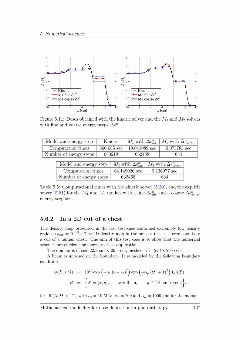
5. Numerical schemes
0 2 4 6 8 10 12x (cm)
0
1
2
3
4
5
6
D /
Ne
KineticM1 fine ∆εn
M1 coarse ∆εn
0 2 4 6 8 10 12x (cm)
0
1
2
3
4
5
6
D /
Ne
KineticM2 fine ∆εn
M2 coarse ∆εn
Figure 5.11: Doses obtained with the kinetic solver and the M1 and M2 solverswith fine and coarse energy steps ∆ǫn.
Model and energy step Kinetic M1 with ∆ǫnair M1 with ∆ǫnwaterComputation times 860.685 sec 19.041089 sec 0.073788 sec
Number of energy steps 683219 632468 634
Model and energy step M2 with ∆ǫnair M2 with ∆ǫnwaterComputation times 64.149026 sec 0.136977 sec
Number of energy steps 632468 634
Table 5.5: Computational times with the kinetic solver (5.20), and the explicitsolver (5.51) for the M1 and M2 models with a fine ∆ǫnair and a coarse ∆ǫnwaterenergy step size.
5.6.2 In a 2D cut of a chest
The density map presented in the last test case contained extremely low densityregions (ρair = 10−3). The 2D density map in the present test case corresponds toa cut of a human chest. The aim of this test case is to show that the numericalschemes are efficient for more practical applications.
The domain is of size 22.3 cm × 29.5 cm, meshed with 223 × 295 cells.A beam is imposed on the boundary. It is modeled by the following boundary
condition
ψ(X, ǫ,Ω) = 1010 exp(
−αǫ (ǫ− ǫ0)2)
exp(
−αµ (Ω1 + 1)2)
1B(X),
B =
X = (x, y), x = 0 cm, y ∈ [18 cm, 20 cm]
.
for all (X,Ω) ∈ Γ−, with ǫ0 = 10 MeV, αǫ = 200 and αµ = 1000 and for the moment
Mathematical modelling for dose deposition in photontherapy 167

5.6. Tests with fast characteristics
models
ψnlmax,m = 1010 exp(
−αǫ (ǫn − ǫ0)2) ⟨
m(Ω) exp(
−αµ (Ω1 + 1)2)⟩
1B(Xl,m),
ψnl,0 = ψn0,m = ψnl,mmax= 0
RCard(m) .
This case is meant to test the relaxation method and the numerical schemes for therelaxed equations. Especially the influence of the choice of the relaxation parameter,i.e. with the caretesian, diagonal or star relaxation directions, is tested on thisproblem.
The dose results obtained with coarse energy steps ∆ǫwater (5.54) using theexplicit scheme are compared to the result with fine energy steps ∆ǫair (5.53).
The isodose curves of 5% (red), 10% (orange), 25% (green), 50% (light blue),70% (dark blue) and 80% (violet) of the maximum dose are plotted on Fig. 5.12over the density map in grayscale. The computational times for this test case aregathered in Table 5.6.
Figure 5.12: Isodose curves in a chest at 5% (red), 10% (yellow), 25% (green),50% (cyan) and 80% (blue) of the maximum dose with a fine ∆ǫn (left) anda coarse ∆ǫn using cartesian (middle left), diagonal (middle right) and star(right) directions of relaxation.
The isocurves of absolute error compared to the explicit scheme with a fineenergy step ∆ǫnair at 0.2% (yellow), 0.5% (light blue), 1% (red) are plotted on Fig.5.13.
The dose obtained with the explicit scheme with coarse energy steps ∆ǫnwaterwith cartesian directions of relaxation with the approximated M1 and M2 modelsare compared to a reference Monte Carlo results of Fig. 5.14, and the computationaltimes are gathered in Table 5.14.
The shape of the dose obtained with the different relaxation parameters with acoarse ∆ǫnwater are close to the one obtained with the cartesian relaxation parameterswhen using fine ∆ǫnair. The absolute error is smaller than 5.3140% of the maximumdose when using the cartesian directions of relaxation, than 12.702% with the diago-nal directions, and than 3.4072% with the star directions. The maximum errors are
168 T. Pichard

5. Numerical schemes
Relaxation directions and ∆ǫn Cartesian, ∆ǫnair Cartesian, ∆ǫnwaterComputation times 5939.6982 sec 20.8869 sec
Number of energy steps 247930 885
Relaxation directions and ∆ǫn Diagonal, ∆ǫnwater Star, ∆ǫnwaterComputation times 22.6130 sec 61.2220 sec
Number of energy steps 885 1768
Table 5.6: Computational times with the explicit solver (5.51) with the differ-ent relaxation directions and the different energy step sizes.
Figure 5.13: Isodose curves of absolute error compared to the dose obtainedwith explicit scheme with fine energy steps ∆ǫnair in a chest at 0.5% (red), 1%(yellow) and 2% (green) of the maximum dose with coarse energy steps ∆ǫn
with cartesian (left), diagonal (middle) and star (right) directions of relaxation.
Solver Monte Carlo M1 model M2 model
Computation times 14 hours 20.8869 sec 74.3470 sec
Table 5.7: Computational times with the Monte Carlo solver, and the explicitsolver (5.51) for the M1 and M2 models using the Cartesian directions ofrelaxation.
located in the middle of the medium at about 2 cm and 6 cm depth and on each sideof the beam at the entry of the low density regions (lungs). When using the diagonal
Mathematical modelling for dose deposition in photontherapy 169

5.7. An implicit scheme for linear equations
Figure 5.14: Isodose curves in a chest at 5% (red), 10% (yellow), 25% (green),50% (cyan) and 80% (blue) of the maximum dose with a Monte Carlo solver(left), with the explicit scheme with coarse energy steps ∆ǫn for the M1 model(middle) and M2 model (right) with cartesian directions of relaxations.
directions of relaxation, the information is transported in diagonal direction. Thus,when transporting particles along the x-axis, the scheme does not transport themfrom one cell to its neighboor. This results in some irregularities which can be seenin Fig. 5.13. The relaxed models are better when the directions of relaxation arecollinear to the mesh directions (i.e. cartesian directions).
Using a the numerical schemes with coarse energy steps provides a significantspeed-up factor compared to the reference method and it provides a relatively goodaccuracy compared to those reference results.
The Cartesian directions of relaxation provides more accurate results than thediagonal and the star directions of relaxation. Therefore, Cartesian directions ofrelaxations are chosen for the next 2D tests.
5.7 An implicit scheme for linear equations
The last approach consists in treating implicitly the non-linear flux term in thetransport equations.
170 T. Pichard

5. Numerical schemes
5.7.1 For the toy problem
On the homogeneous relaxed equations (5.30), such a scheme simply reads
1 +∆ǫn
ρl− 12∆x
(f1τ )n+1l = (f1
τ )nl +∆ǫn
ρl− 12∆x
(f τ1 )n+1l−1 = 0,
1 +∆ǫn
ρl+ 12∆x
(f2τ )n+1l = (f2
τ )nl +∆ǫn
ρl+ 12∆x
(f τ2 )n+1l+1 = 0,
which can be obtained e.g. by a Finite Difference approach. When applying thisscheme to (5.30) in the relaxation method, this scheme leads to write the followingscheme for ψ
ψn+1l − ∆ǫn
∆x
Fn+1l+ 1
2
ρl+ 12
−Fn+1l− 1
2
ρl− 12
= ψnl , (5.55a)
Fn+1l+ 1
2
=1
2
[
F(ψn+1l+1 ) + F(ψn+1
l ) + (ψn+1l+1 −ψn+1
l )]
. (5.55b)
which equivals to rewriting (5.9) with implicit fluxes.
5.7.2 For the transport equations
When applied to the transport equations of electrons (5.2), this scheme reads
(
Sn+1Id− ∆ǫnMn+1)
ψn+1l +
∆ǫn
∆x
Fn+1l+ 1
2
ρl+ 12
−Fn+1l− 1
2
ρl− 12
= Snψnl , (5.56a)
Fn+1l+ 1
2
=1
2
[
F(ψn+1l+1 ) + F(ψn+1
l ) − (ψn+1l+1 −ψn+1
l )]
, (5.56b)
Such a discretization can also be applied for the transport of both photons andelectrons (5.4), i.e. to the relaxed equation (5.33). This leads to write the numericalscheme
An+1γ→γψγ
n+1l +
∆ǫn
∆x
Fγn+1l+ 1
2
ρl+ 12
−Fγ
n+1l− 1
2
ρl− 12
=n∑
n′=1
Bn′,n+1C,γ ψγ
n′
l (5.57a)
An+1e→eψe
n+1l +
∆ǫn
∆x
Fen+1l+ 1
2
ρl+ 12
−Fe
n+1l− 1
2
ρl− 12
=n∑
n′=1
Bn′,n+1e→e ψe
n′
l +Bn′,n+1γ→e ψγ
n′
l ,
(5.57b)
for α = γ, e Fαn+1l+ 1
2
=1
2
[F(ψα
n+1l+1 ) + F(ψα
n+1l ) − (ψα
n+1l+1 −ψαn+1
l )], (5.57c)
Mathematical modelling for dose deposition in photontherapy 171

5.7. An implicit scheme for linear equations
where the matrices An+1γ→γ , An+1
e→e, Bn′,n+1γ→γ , Bn′,n+1
e→e and Bn′,n+1γ→e read
An+1γ→γ = σn+1
T,C Id− sn+1,n+1C,γ ∆ǫn, Bn′,n+1
γ→γ = sn′,n+1C,γ ∆ǫn
′
,
An+1e→e =
Sn+1
∆ǫnId−Mn+1, Bn′,n+1
γ→e = sn′,n+1C,e ∆ǫn
′
,
Bn′,n+1e→e =
SnId
∆ǫnδn′,n,
In 2D, this numerical scheme reads
An+1γ→γψγ
n+1l,m +
∆ǫn
∆x
Fγn+1l+ 1
2,m
ρl+ 12,m
−Fγ
n+1l− 1
2,m
ρl− 12,m
+∆ǫn
∆y
Fγn+1l,m+ 1
2
ρl,m+ 12
−Fγ
n+1l,m− 1
2
ρl,m− 12
=n∑
n′=1
Bn′,n+1C,γ ψγ
n′
l,m (5.58a)
An+1e→eψe
n+1l,m +
∆ǫn
∆x
Fen+1l+ 1
2,m
ρl+ 12,m
−Fe
n+1l− 1
2,m
ρl− 12,m
(5.58b)
+∆ǫn
∆y
Fen+1l,m+ 1
2
ρl,m+ 12
−Fe
n+1l,m− 1
2
ρl,m− 12
=n∑
n′=1
Bn′,n+1e→e ψe
n′
l,m +Bn′,n+1γ→e ψγ
n′
l,m,
for α = γ, e, Fαn+1l+ 1
2,m
=1
2
[F(ψα
n+1l+1,m) + F(ψα
n+1l,m ) − (ψα
n+1l+1,m −ψαn+1
l,m )],
(5.58c)
Fαn+1l,m+ 1
2
=1
2
[F(ψα
n+1l,m+1) + F(ψα
n+1l,m ) − (ψα
n+1l,m+1 −ψαn+1
l,m )].
(5.58d)
5.7.3 Computing ψn+1l
The numerical schemes (5.56), (5.56), (5.57) and (5.58) can be rewritten under theform
J(ψn+1)l = Rnl , (5.59)
where J is a non-linear function of the unknown ψn+1 and Rnl contains all the terms
ψn′
for n′ < n+ 1. In order to use the implicit schemes, the function J needs to beinvertible and its inverse needs to be realizable.
In order to compute ψn+1 and to prove the existence of a realizable solution to(5.59), an iterative method can be used. This method is inspired of [13].
Rewrite (5.59) under the form
−L(ψn+1l−1 ) +D(ψn+1
l ) −R(ψn+1l+1 ) = Rn
l , (5.60)
172 T. Pichard

5. Numerical schemes
where L(ψn+1l−1 ), respectively D(ψn+1
l ) and R(ψn+1l+1 ), contains all the terms depend-
ing of ψn+1l−1 , respectively ψn+1
l and ψn+1l+1 . When applied to (5.56), this reads
L(ψn+1l−1 ) =
∆ǫn
ρl− 12∆x
ψn+1l−1 − F
(
ψn+1l−1
)
2, (5.61a)
R(ψn+1l+1 ) =
∆ǫn
ρl+ 12∆x
ψn+1l+1 + F
(
ψn+1l+1
)
2, (5.61b)
D(ψn+1l ) =
1 +∆ǫn
∆x
1
ρl− 12
+1
ρl+ 12
ψn+1l , (5.61c)
Rnl = ψnl , (5.61d)
when applied to (5.56), this reads
L(ψn+1l−1 ) =
∆ǫn
ρl− 12∆x
ψn+1l−1 − F
(
ψn+1l−1
)
2, (5.62a)
R(ψn+1l+1 ) =
∆ǫn
ρl+ 12∆x
ψn+1l+1 + F
(
ψn+1l+1
)
2, (5.62b)
D(ψn+1l ) =
Sn+1 +∆ǫn
∆x
1
ρl− 12
+1
ρl+ 12
Id− ∆ǫnMn+1
ψn+1l ,(5.62c)
Rnl = Snψnl , (5.62d)
and when applied to (5.57), this reads
L(ψn+1l−1 ) =
∆ǫn
ρl− 12∆x
ψγn+1l−1 − F
(
ψγn+1l−1
)
2,
∆ǫn
ρl− 12∆x
ψen+1l−1 − F
(
ψen+1l−1
)
2
,
(5.63a)
R(ψn+1l+1 ) =
∆ǫn
ρl+ 12∆x
ψγn+1l+1 + F
(
ψγn+1l+1
)
2,
∆ǫn
ρl+ 12∆x
ψen+1l+1 + F
(
ψen+1l+1
)
2
,
(5.63b)
D(ψn+1l ) =
An+1γ→γ +
∆ǫnId
∆x
1
ρl− 12
+1
ρl+ 12
ψγn+1l , (5.63c)
An+1e→e +
∆ǫnId
∆x
1
ρl− 12
+1
ρl+ 12
ψen+1l +An+1
γ→eψγn+1l
,
Rnl =
(n∑
n′=1
Bn′n+1γ→γ ψγ
n′
,n∑
n′=1
Bn′n+1e→e ψe
n′
+Bn′n+1γ→e ψγ
n′
)
. (5.63d)
Remark that in each case the diagonal term D is linear and can be invertednumerically. The following iterative algorithm can be used to compute the solutionof (5.59).
Mathematical modelling for dose deposition in photontherapy 173

5.7. An implicit scheme for linear equations
Algorithm 5.1Initialization: Set
ψn+1,(0)l = ψnl ∀l. (5.64)
Iteration: Solve iteratively
ψn+1,(k+1)l = D−1
(
Rnl + L(ψ
n+1,(k)l−1 ) +R(ψ
n+1,(k)l+1 )
)
, (5.65)
until the following residual error
r(k) =∥∥∥D(ψ
n+1,(k)l−1 ) − Rn
l − L(ψn+1,(k)l−1 ) −R(ψ
n+1,(k)l+1 )
∥∥∥
∞(5.66)
reaches a desired values maximum values rmax or until k reaches a maximumvalue kmax.
Proposition 5.4 Suppose ψn′
l is realizable for all l and all n′ < n+ 1.Then there exists a unique set of realizable vectors (ψn+1)l=1,...,lmax satisfying(5.59) for all l.
Moreover the algorithm 5.1 converges to this solution and ψn+1,(k+1)l ∈ Rm is
realizable for all l at each step (k).
Proof The Jacobian of J is a block matrix which is defined by
(∂J(ψ)
∂ψ
)
l,k
=∂J(ψ)l∂ψk
= D−1
[
∂L
∂ψl−1
(ψl−1)δk,l−1 +∂R
∂ψl+1
(ψl+1)δk,l+1
]
.
Then using a Gershgörin theorem for block matrices ([25]) leads to writethat all the eigenvalues of the Jacobian of J are bounded by
Sp
(∂J(ψ)
∂ψ
)
⊂ [−r,+r],
r = |||D|||−1 maxl
(∂L
∂ψl(ψl) +
∂R
∂ψl(ψl)
)
.
The eigenvalues of the Jacobians ∂L∂ψl
and ∂R∂ψl
can be bounded using Lemma 5.1.
Comparing those eigenvalues to |||D|||−1, where D is given by (5.61), (5.62) or(5.63), leads to write that the spectral radius r is strictly inferior to 1. Thisimplies that the function J is contractant, so it has a unique fixed point, andAlgorithm 5.1 converges to this fixed point.
It remains to verify that ifψn,(k)l is realizable for all l, thenψn,(k+1)
l = J(ψn,(k)l )
remains realizable.By assumption ψn = ψn+1,(0) is realizable. As Rn
l is a positive combinationof realizable vectors, it is also realizable.
Then, by iteration, if ψn+1,(k)l is realizable for all l, then L(ψ
n+1,(k)l ) and
174 T. Pichard

5. Numerical schemes
R(ψn+1,(k)l ) are realizable (according to Proposition 5.1), and it remains to prove
that D−1 preserves realizability.In the case of the toy problem (5.55), D = αId with α > 0, therefore
the realizability is obviously preserved. In the case of the electron transport(5.56), it was proven in Proposition 5.2. And in the case of coupled photonsand electrons transport (5.57), it can be proven by reproducing the proof ofProposition 5.2.
Remark 5.5 The iterative method proposed in Algorithm 5.1 can be seen asa Jacobi method with non-linear extra-diagonal terms L and R. Similarily, aGauss-Seidel method for this non-linear problem can be written. It consists insolving alternatively
ψn+1,(k+1)l = D−1
(
Rnl + L(ψ
n+1,(k)l−1 ) +R(ψ
n+1,(k+1)l+1 )
)
, (5.67a)
ψn+1,(k+1)l = D−1
(
Rnl + L(ψ
n+1,(k+1)l−1 ) +R(ψ
n+1,(k)l+1 )
)
, (5.67b)
instead of (5.65) in Algorithm 5.1. This algorithm was tested experimentallyand converged to the desired state. However, it was not proven to be convergentat the theoretical level.
5.8 Tests on the implicit solver
The aim of those test is to study the implicit scheme (5.57). Especially, two conver-gence rates are studied: the convergence of Algorithm (5.1) according to the numberkmax of iterations to reach the resdual rmax, and the convergence of the nummericalscheme according to the cells size ∆ǫn and ∆x.
Two test cases are proposed, a 1D electron beam and a 2D photon beam.
5.8.1 A 1D electron beam
This test case is identical to the one in Subsection 5.3.1, but only the implict solver(5.57) is used. However, as the implicit numerical scheme is more flexible than theexplicit one, all the physics of the electronic collisions described by Equation 5.4 wasincluded for this test case.
The objective of this subsection is only to study the convergence rates. Doseresults obtained with Algorithm 5.1 are presented in the next subsection.
Convergence of Algorithm 5.1
The number of spatial cells is fixed at 600 and the energy step is fixed by
∆ǫn = 5Sn∆x, (5.68)
with an initial energy ǫmax = 1.2ǫ0 = 12 MeV and a final energy at ǫmin = 10−3
MeV.
Mathematical modelling for dose deposition in photontherapy 175

5.8. Tests on the implicit solver
The iterative method of Algorithm 5.1 requires a criterium to stop. Either thenumber of iterations kmax is fixed or the residual (5.66) is reached.
As a first test, the number of iterations kmax is fixed at different values, i.e. 10,30, 50 and 70, and the residual rn,kmax is plotted as a function of the energy stepn on Fig. 5.15. As a second test, the maximum residual rmax is fixed at differentvalues, i.e. 0.1, 0.01, 0.001 and 0.0001, and the number of iterations k required toreach this residual is plotted as a function of the energy step n on Fig. 5.16.
0 20 40 60 80 100Step n
0
50
100
150
200
Num
ber
of it
erat
ions
k
rmax
= 0.0001rmax
= 0.001rmax
= 0.01rmax
= 0.1
Figure 5.15: Number of iterations kas a function of the energy step n fora given maximum residual rmax
0 50 100Step n
1
100
10000
1e+06
1e+08
1e+10
Fina
l res
idua
l rn,
k max
kmax
= 10k
max = 30
kmax
= 50k
max = 70
Figure 5.16: Final residual rn,kmax asa function of the energy step n for agiven number of iterations kmax
During the first steps (up to n = 8), the values of ψ on the boundary (see (5.25))is very low and the fluence ψ inside the medium is negligible. Therefore the valuesof k and of rn,kmax are also very low.
In the first steps where the values of ψ is non-negligible, Algorithm 5.1 requiresa large number of iterations to converge. At those energy the energy derivative∂ǫψ ≡ (ψn − ψn+1)/∆ǫn is large and the intialization ψn+1,(0) = ψn of Algorithm5.1 is inaccurate which forces the algorithm to make more iterations to converge.
The convergence rate progressively raises, i.e. the final residual rn,kmax or thenumber of itarations k reduce.
Finally, near the end of the simulation, the particles leave the system by reachingan energy lower than threshold ǫmin. As the fluence ψ drops, the energy derivativetoo and the algorithm requires less iterations to converge. This explains the finaldrop in Fig. 5.15 and 5.16.
Convergence of the numerical scheme
Based on the construction of the implicit scheme (5.57), one may expect the trun-cation error to be of order 1 in ∆x and in ∆ǫn.
The energy step size is fixed by the condition (5.68).No analytical solution is known for equations (5.4). Therefore the solution obtain
with the implicit scheme with different grid sizes are compared to a reference thatwas computed with this same scheme with a large number of cells, i.e. lmax = 9600.
176 T. Pichard

5. Numerical schemes
The number of spatial cells lmax is chosen to be 300, 600, 1200, 2400 and 4800cells and for the reference solution 9600 cells.
The convergence rate of the numerical scheme is represented through the discreteL2 error between the reference solution ψ computed with 9600 spatial cells and theless refined results. This error is plotted on Fig. 5.17 as a function of ∆x. On this
0,001 0,01 ∆x
1e+08
Err
or
Error of the implicit schemeError of order 1
Figure 5.17: Discrete L2 error compared to the most refined solution as afunction of ∆x.
test case, one obtains an experimental convergence rate in ∆x of 1.1046894.
5.8.2 Comparison with the explicit solver
This test case is identical to the 1D test case containing slabs of air of Subsection5.6.1. The same parameters are used, i.e. 1200 spatial cells, the same beam (5.25),and the energy step ∆ǫn is fixed either to ∆ǫnwater (5.54) or to ∆ǫnair (5.53).
The aim of this case is only to compare the explicit (5.51) and implicit (5.56)numerical schemes. For this purpose, only the M1 results are shown.
The maximum residual (5.66) for the implicit scheme (5.56) is fixed at rmax = 103
and the maximum number of iterations is fixed kmax = 10000. Experimentally thisnumber of iterations was never reached, meaning that the maximum residual wasalways reached.
The doses obtained with the M1 model with the explicit (5.51) and implicit(5.56) numerical schemes are plotted on Fig. 5.18 and the computational times aregathered in Table 5.8 and 5.9.
Mathematical modelling for dose deposition in photontherapy 177

5.8. Tests on the implicit solver
0 2 4 6 8 10 12x (cm)
0
1
2
3
4
5D
/ N
e
Explicit with fine stepsExplicit with coarse stepsImplicit with fine stepsImplicit with coarse steps
Figure 5.18: Doses obtained with the M1 model with the explicit and implicitschemes with fine and coarse energy steps ∆ǫn.
Numerical scheme Explicit with ∆ǫnair Implicit with ∆ǫnairComputation times 63.592346 sec 118.435718 sec
Number of energy steps 632468 632468
Table 5.8: Computational times with the explicit (5.51) and implicit (5.56)solver with a fine energy step size ∆ǫnair.
Numerical schemes Explicit with ∆ǫnwater Implicit with ∆ǫnwaterComputation times 0.073788 sec 1.409635 sec
Number of energy steps 634 634
Table 5.9: Computational times with the explicit (5.51) and implicit (5.56)solver with a coarse energy step size ∆ǫnwater.
The difference between the dose results with the explicit and implicit schemeswith a fine energy steps is very small. This shows that both schemes converge tothe same results, which was expected.
As for the explicit scheme, the results with a larger energy step ∆ǫn = ∆ǫnwatershow good agreements with those with a fine ∆ǫn = ∆ǫnair.
The implicit and explicit schemes with coarse steps present an error of the sameorder compared to the results with fine energy steps.
178 T. Pichard

5. Numerical schemes
The implicit scheme requires an interne loop to solve the scheme. It is more flexi-ble (it can be used on equations without hyperbolic operators), however it introducesadditional computational costs and errrors that can be observed on this test case.Remark that with the maximum residual chosen for this test case, i.e. rmax = 103,the error introduced by the iterative method is small enough such that the doseresults are comparable to those of the explicit solver which does not introduce suchan error.
5.8.3 A 2D photon beam
For this test case, photons are injected in a 2D homogeneous water phantom insteadof electrons. The size of the medium is 2 cm × 10 cm, and a 0.5 cm large beam of500 keV photons is injected on the left boundary. This is modeled by the boundarycondition
ψγ(X, ǫ,Ω) = 1010 exp(
−αǫ (ǫ− ǫ0)2)
exp(
−αµ (Ω1 − 1)2)
1B(X), ∀(X,Ω) ∈ Γ−,
B =
X = (x, y), x = 0, y ∈ [1 cm, 2 cm]
.
with ǫ0 = 500 keV, αǫ = 20000 and αµ = 10000 and for the moment models
ψn0,m = 1010 exp(
−αǫ (ǫn − ǫ0)2) ⟨
m(Ω) exp(
−αµ (Ω1 − 1)2)⟩
1B(Xl,m),
ψnl,0 = ψnlmax,m = ψnl,mmax= 0
RCard(m) .
First results
The dose obtained with the M1 and M2 model with the implicit scheme (5.58) arecompared to a reference Monte Carlo results on Fig. 5.19 and the computationaltimes are gathered on Table 5.10.
Solver Monte Carlo M1 solver M2 solver
Computation times 14 hours 49.78699 sec 215.0480 sec
Table 5.10: Computational times with the implicit solver with the Cartesiandirection of relaxation.
The doses along the axis y = 1 cm is plotted Fig. 5.20 and along the axes x = 2cm and x = 8 cm on Fig. 5.21.
The total cross section for photons is much lower than the one for electrons.This implies that the photons collide much less than electrons and therefore travellonger distances without being deflected.
This can be observed on the Monte Carlo results on Fig. 5.19. However, the M1
and M2 results with the implicit scheme are almost identical and are very diffusedin the direction transverse to the beam contrarily to the Monte Carlo results. Thisis due to the relaxation parameters chosen (5.39).
Mathematical modelling for dose deposition in photontherapy 179

5.8. Tests on the implicit solver
Figure 5.19: Doses obtained with the Monte Carlo solver (top) and the ap-proximated M1 (middle) and M2 (below) models.
0 2 4 6 8 10x (cm)
0
0,2
0,4
0,6
0,8
1
D /
Dm
ax
Monte CarloM1M2
Figure 5.20: Dose obtained with the Monte Carlo solver and the approximatedM1 and M2 models along the axis y = 1 cm.
Transverse diffusion
In practice, the relaxation method can be used under the stability condition (5.28)on the relaxation speeds. However, in 1D, the relaxation method is known to be
180 T. Pichard

5. Numerical schemes
0 0,5 1 1,5 2y (cm)
0
0,2
0,4
0,6
0,8
D /
Dm
ax
MC x = 2 cmM1 x = 2 cmM2 x = 2 cm
0 0,5 1 1,5 2y (cm)
0
0,2
0,4
0,6
0,8
D /
Dm
ax
MC x = 8 cmM1 x = 8 cmM2 x = 8cm
Figure 5.21: Dose obtained with the Monte Carlo solver and the approximatedM1 and M2 models along the axes x = 2 cm and x = 8 cm.
overdiffusive when the relaxation speeds λj are too large compared to the eigenvaluesof the Jacobian of the flux ∂ψF(ψ).
Bounds of the eigenvalues of the Jacobian of the fluxes
The relaxation speeds were chosen to be of norm |λj | = 1/ρ which was enough tosatisfy (5.28) according to Lemma 5.1. However, when ψ is the moment vector ofan imperfect beam in the direction e1 modeled by
ψ =
∫
S2m(Ω) exp(−αµ(Ω1 − 1))dΩ,
then the spectral radius of the Jacobian of the flux F2 transverse to the direction ofthe beam is zero. Indeed, define
A := ∂ψF2(ψ),
B := ∂λF2(ψ) =
∫
S2Ω2m(Ω) ⊗ m(Ω) exp(λTm(Ω))dΩ
=
∫
S2Ω2m(Ω) ⊗ m(Ω) exp(−α2(Ω1 − 1))dΩ,
C := ∂λψ =
∫
S2m(Ω) ⊗ m(Ω) exp(λTm(Ω))dΩ
=
∫
S2m(Ω) ⊗ m(Ω) exp(−αµ(Ω1 − 1))dΩ.
Then the eigenvalues αi (associated to the eigenvector Vi) of the Jacobian of theflux F2 can be bounded
BWi = αiCWi, Wi = C−1Vi,
BWi.Wi =
∫
S2Ω2(m(Ω)TWi)
2 exp(−αµ(Ω1 − 1))dΩ = 0,
CWi.Wi =
∫
S2(m(Ω)TWi)
2 exp(−αµ(Ω1 − 1))dΩ > 0.
Mathematical modelling for dose deposition in photontherapy 181

5.8. Tests on the implicit solver
Therefore all the eigenvalues αi of the Jacobian of the transverse flux are zero.
In a more general way, those eigenvalues can be computed in the case of the M1
model. Consider that ψ1 is colinear to e1 (otherwise just use a rotation to workin such a reference frame). Using the form (4.26) of the closure, the fluxes in thedirection e1 and in the transverse direction e2 read
ψ =(
ψ0, ψ1)
,
Fn(ψ) =
(
ψ1.n,ψ0
2
[
(1 − χ2)n+ (3χ2 − 1)(ψ1.n)ψ1
|ψ1|2
])
,
∂ψ (Fn(ψ)) =
(
0 V1
V2 M
)
, (5.69)
V1 = ∂ψ1(ψ1.n) = (n1, n2, n3) ,
V2 = ∂ψ0
(
ψ0
2
[
(1 − χ2)n+ (3χ2 − 1)(ψ1.n)ψ1
|ψ1|2
])
,
=1
2
[
(1 − χ2)n+ (3χ2 − 1)(ψ1.n)ψ1
|ψ1|2
]
− |ψ1|2ψ0
χ′2
(
−n+ 3(ψ1.n)ψ1
|ψ1|2
)
,
M = ∂ψ1
(
ψ0
2
[
(1 − χ2)n+ (3χ2 − 1)(ψ1.n)ψ1
|ψ1|2
])
=χ′
2
2
ψ1
|ψ1| ⊗(
−n+ 3(ψ1.n)ψ1
|ψ1|2
)
+ψ0
2(3χ2 − 1)
(
n⊗ ψ1
|ψ1|2 +ψ1.n
|ψ1|2 Id− 2(ψ1.n)ψ1 ⊗ ψ1
|ψ1|4
)
.
Chose a reference frame such that ψ1 = ψ11e1 with ψ1
1 ≥ 0. In this referenceframe, the Jacobian of the flux F1 along the direction e1 reads
∂ψ (F1(ψ)) =
0 1 0 0χ2 −N1
1χ′2 χ′
2 0 0
0 0 3χ2−12N1
10
0 0 0 3χ2−12N1
1
,
and so the spectrum of the Jacobian of the flux is
Sn(N11 ) = Sp (∂ψ (F(ψ)e1))
=
(3χ2 − 1
2N11
,3χ2 − 1
2N11
,
χ′2 +
√
χ′22 + 4(χ2 −N1
1χ′2)
2,χ′
2 −√
χ′22 + 4(χ2 −N1
1χ′2)
2
.
182 T. Pichard

5. Numerical schemes
Now computing the Jacobian of the flux in a transverse direction, e.g. e2 reads
∂ψ (F2(ψ)) =
0 0 1 0
0 0χ′
22 0
1−χ2+N11χ
′2
23χ2−12N1
10 0
0 0 0 0
,
and so the spectrum of the Jacobian of the flux is
St(N11 ) = Sp (∂ψ (F2(ψ)))
=
0, 0,
√√√√
1 − χ2 +N11χ
′2 − 3χ2−1
2N11χ′
2
2, −
√√√√
1 − χ2 +N11χ
′2 − 3χ2−1
2N11χ′
2
2
.
Now, in order to come back to the computations in any reference frame, one cansimply use a rotation R such that Rψ1 = ψ1
1e1. One has
∂ψ (Fn(ψ)) = ∂(ψ0,Rψ11e1)
(
Fn(ψ0, Rψ11e1)
)
= R2∂ψFRTn
(
ψ0, |ψ1|e1
)
RT2 ,
R2 =
(
1 0R3
0R3 R
)
.
The spectrum of such a matrix can be bounded using the previous computations
Sp (∂ψ (Fn(ψ))) ⊂ [b−, b+], (5.70a)
b−(N1, n) = (1 − θ) minSt(|N1|) + θminSn(|N1|), (5.70b)
b+(N1, n) = (1 − θ) maxSt(|N1|) + θmaxSn(|N1|), (5.70c)
θ =N1.n
|N1| .
Remark that those bounds b− and b+ are not the exact minimum and maximumeigenvalues of the Jacobians of the flux, which could be computed analyticallythrough (5.69). Although computing numerically such eigenvalues using the an-alytical formulae introduces errors which can be non-negligible, while computingthe bounds in (5.70) is easier. Furthermore, those bounds b− and b+ are sufficientfor the present applications. Indeed, one verifies that they are zero when consideringthe flux of a perfect beam in the transverse direction of this beam.
Mathematical modelling for dose deposition in photontherapy 183

5.8. Tests on the implicit solver
The modified relaxation parameters
Now one can propose new relaxation parameters by replacing those bounds in thedefinition of the Cartesian parameter of relaxation, e.g.
Relaxation directions λ1 = (b1, 0) , λ2 = (b2, 0) , (5.71a)
λ3 = (0, b3) , λ4 = (0, b4) ,
Associated Maxwellians M1 =|b1|ψ
2(|b1| + |b2|) +Fλ1
|λ1|(|b1| + |b2|) , (5.71b)
M2 =|b2|ψ
2(|b1| + |b2|) +Fλ2
|λ2|(|b1| + |b2|) , (5.71c)
M3 =|b3|ψ
2(|b3| + |b4|) +Fλ3
|λ3|(|b3| + |b4|) , (5.71d)
M4 =|b4|ψ
2(|b3| + |b4|) +Fλ4
|λ4|(|b3| + |b4|) . (5.71e)
All the schemes based on the relaxation methods require that the MaxwelliansMi ∈ Rm are realizable as long as ψ ∈ Rm. In practice, this implies that there isan additional requirement on the bounds b1, b2, b3 and b4.
For the M1 model, those requirements can easily be computed using (3.41), itreads
( |bi|2
+N1.λi|λi|
)2
>
∣∣∣∣
|bi|2N1 +N2 λi
|λi|
∣∣∣∣
2
,
and therefore
|bi| > max
(
0, bmin
(
N1,λi|λi|
))
,
bmin(N1, n) :=−β −
√
β2 − αγ
α,
α =1 − |N1|2
4, β =
1
2
(
N1.n−N1.(N2n))
, γ = (N1.n)2 − |N2n|2.
This leads to fix the bounds
b1(ψ) = max(
10−8, b+(N1, e1), bmin(N1, e1))
,
b2(ψ) = min(
−10−8, b−(N1, e1), −bmin(N1,−e1))
,
b3(ψ) = max(
10−8, b+(N1, e2), bmin(N1, e2))
,
b4(ψ) = min(
−10−8, b−(N1, e2), −bmin(N1,−e2))
,
where the constants ±10−8 are chosen arbitrarily low to avoid divisions by zero.
184 T. Pichard

5. Numerical schemes
The new numerical scheme
Using the Maxwellians (5.71) leads to rewrite the fluxes
Fn+1l+ 1
2,m
=1
|bn+11,l+ 1
2,m
| + |bn+12,l+ 1
2,m
|
[
|bn+12,l+ 1
2,m
|F(ψn+1l+1,m)e1 + |bn+1
1,l+ 12,m
|F(ψn+1l,m )e1
+|bn+11,l+ 1
2,mbn+1
2,l+ 12,m
|(ψn+1l+1,m −ψn+1
l,m )
]
,
Fn+1l,m+ 1
2
=1
|bn+13,l,m+ 1
2
| + |bn+14,l,m+ 1
2
|
[
|bn+14,l,m+ 1
2
|F(ψn+1l,m+1)e2 + |bn+1
3,l,m+ 12
|F(ψn+1l,m )e2
+|bn+13,l,m+ 1
2
bn+14,l,m+ 1
2
|(ψn+1l,m+1 −ψn+1
l,m )
]
,
bn+11,l+ 1
2,m
= max(
b1(ψn+1l,m ), b1(ψn+1
l+1,m))
, bn+12,l+ 1
2,m
= min(
b2(ψn+1l,m ), b2(ψn+1
l+1,m))
,
bn+13,l,m+ 1
2
= max(
b3(ψn+1l,m ), b3(ψn+1
l+1,m))
, bn+14,l,m+ 1
2
= min(
b4(ψn+1l,m ), b4(ψn+1
l+1,m))
,
in the implicit numerical scheme (5.58) which turns into
Rnl,m = −L1(ψn+1
l−1,m) − L2(ψn+1l,m−1) +D(ψn+1
l,m ) (5.72)
−R1(ψn+1l−1,m) −R2(ψn+1
l,m−1), (5.73)
where the rest term reads
Rnl,m =
(n∑
n′=1
Bn′n+1γ→γ ψγ
n′
l,m,n∑
n′=1
Bn′n+1e→e ψe
n′
l,m +Bn′n+1γ→e ψγ
n′
l,m
)
,
the operators L1, L2, R1 and R2 read
L1(ψn+1l−1,m) =
(
c1ψγn+1l−1,m − a1F1
(
ψγn+1l−1,m
)
, c1ψen+1l−1,m − a1F1
(
ψen+1l−1,m
))
,
L2(ψn+1l,m−1) =
(
c2ψγn+1l,m−1 − a2F2
(
ψγn+1l,m−1
)
, c2ψen+1l,m−1 − a2F2
(
ψen+1l,m−1
))
,
R1(ψn+1l+1,m) =
(
c3ψγn+1l+1,m + a3F1
(
ψγn+1l+1,m
)
, c3ψen+1l+1,m + a3F1
(
ψen+1l+1,m
))
,
R2(ψn+1l,m+1) =
(
c4ψγn+1l,m+1 + a4F2
(
ψγn+1l,m+1
)
, c4ψen+1l,m+1 + a4F2
(
ψen+1l,m+1
))
.
With this particular choice of bounds bi, the operator D is not necessarily linear.Indeed it reads
D(ψn+1l,m ) =
((
An+1γ→γ + (c1 + c2 + c3 + c4)Id
)
ψγn+1l,m
+(a1 − a3)F2(ψγn+1l,m ) + (a2 − a4)F2(ψγ
n+1l,m ),
(
An+1e→e + (c1 + c2 + c3 + c4)Id
)
ψen+1l,m +An+1
γ→eψγn+1l,m
+(a1 − a3)F1(ψen+1l,m ) + (a2 − a4)F2(ψe
n+1l,m )
)
,
Mathematical modelling for dose deposition in photontherapy 185

5.8. Tests on the implicit solver
which is non-linear when a1 6= a3 or a2 6= a3. In those computations, the scalars aiand ci read
a1 =∆ǫn
ρl− 12,m∆x
|bn+11,l− 1
2,m
|
|bn+11,l− 1
2,m
| + |bn+12,l− 1
2,m
|, c1 = a1|bn+1
2,l− 12,m
|,
a2 =∆ǫn
ρl,m− 12∆y
|bn+13,l,m− 1
2
|
|bn+13,l,m− 1
2
| + |bn+14,l,m− 1
2
|, c2 = a2|bn+1
4,l,m− 12
|,
a3 =∆ǫn
ρl+ 12,m∆x
|bn+12,l+ 1
2,m
|
|bn+11,l+ 1
2,m
| + |bn+12,l+ 1
2,m
|, c3 = a3|bn+1
1,l+ 12,m
|,
a4 =∆ǫn
ρl,m+ 12∆y
|bn+14,l,m+ 1
2
|
|bn+13,l,m+ 1
2
| + |bn+14,l,m+ 1
2
|, c4 = a4|bn+1
3,l,m+ 12
|.
The new operator D is non-linear and is therefore not trivial to inverse. In orderto use Algorithm 5.1 with those operators, D is decomposed into a linear and anon-linear part under the form
D(ψ) = Di(ψ) −De(ψ), (5.74)
Di(ψ) =((
An+1γ→γ + (c1 + c2 + c3 + c4 + α)Id
)
ψγ ,(
An+1e→e + (c1 + c2 + c3 + c4 + α)Id
)
ψe +An+1γ→eψγ
)
,
De(ψ) = (αψγ − (a1 − a3)F (ψγ)e1 − (a2 − a4)F (ψγ)e2,
αψe − (a1 − a3)F (ψe)e1 − (a2 − a4)F (ψe)e2) ,
where the coefficient α is chosen such that the operator De preserves the realizability.In practice, the following coefficient α is chosen
α = |a1 − a3| + |a2 − a4|.
Finally, Algorithm 5.1 is rewritten by replacing (5.65) by
ψn+1,(k+1)l,m = D−1
i
(
Rnl,m + L1(ψn+1,(k)l−1,m ) + L2(ψ
n+1,(k)l,m−1 )
+De(ψn+1,(k)l,m ) +R1(ψ
n+1,(k)l−1,m ) +R2(ψ
n+1,(k)l,m−1
)
.
One verifies that this modified algorithm is still convergent and preserves realizabil-ity.
Computing the eigenvalues of the Jacobian of the flux is more difficult, and thismethod was only tested for the M1 model.
The dose results with the modified scheme
Using this modified algorithm on the 2D photon beam test case provides the doseresult on Fig. 5.22 with the computational times in Table 5.11.
186 T. Pichard

5. Numerical schemes
Figure 5.22: Doses obtained with the Monte Carlo solver (top) and the approx-imated M1 model with the original Cartesian (middle) and modified (below)relaxation parameters.
Solver Monte Carlo M1 solver modified M1 solver
Computation times 14 hours 49.78699 sec 204.1239 sec
Table 5.11: Computational times with the implicit solver with the Cartesianparameters of relaxation and the modified ones.
The dose along the axis y = 1 cm is plotted on Fig. 5.23 and along the axesx = 2 cm and x = 8 cm on Fig. 5.24.
The dose results with the modified relaxation parameters are much closer to thereference Monte Carlo results. The dose is not diffused in the tranverse directionwhich is the expected results. The plots along the transverse direction show thatthe diffusion phenomenum is accurately modeled when using the modified relaxationparameters.
Due to the noise in the Monte Carlo and the normalization by maxD, the M1
dose curves with the modified relaxation parameters are slightly above the MonteCarlo reference.
Remark that the computational time is higher with the modified relaxation pa-rameters. When dividing the operator D in two parts (5.74) in order to enforcethe preservation of the realizability, a parameter αId was artificially added on bothsides of (5.73). This method stabilizes the algorithm, but it reduces the convergencerate which explains the difference of computational times. The computational times
Mathematical modelling for dose deposition in photontherapy 187

5.8. Tests on the implicit solver
0 2 4 6 8 10x (cm)
0
0,2
0,4
0,6
0,8
1
D /
Dm
ax
Monte CarloM1 Cartesian relaxation parametersM1 modified relaxation parameters
Figure 5.23: Doses obtained with the Monte Carlo solver and the approximatedM1 model with the Cartesian and the modified relaxation parameters alongthe axis y = 1 cm.
0 0,5 1 1,5 2y (cm)
0
0,2
0,4
0,6
0,8
D /
Dm
ax
MC x = 2 cmM1 Cartesian x = 2 cmM1 modified x = 2 cm
0 0,5 1 1,5 2y (cm)
0
0,2
0,4
0,6
0,8
D /
Dm
ax
MC x = 8 cmM1 Cartesian x = 8 cmM1 modified x = 8 cm
Figure 5.24: Doses obtained with the Monte Carlo solver and the approximatedM1 model with the Cartesian and the modified relaxation parameters alongthe axes x = 2 cm and x = 8 cm.
with this method is still much lower than with the Monte Carlo reference.
188 T. Pichard

Bibliography
[1] G. W. Alldredge, C. D. Hauck, D. P. O’Leary, and A. L. Tits. Adaptive changeof basis in entropy-based moment closures for linear kinetic equations. J. Com-put. Phys., 74(4), february 2014.
[2] G. W. Alldredge, C. D. Hauck, and A. L. Tits. High-order entropy-basedclosures for linear transport in slab geometry II: A computational study of theoptimization problem. SIAM J. Sci. Comput., 34(4):361–391, 2012.
[3] D. Aregba-Driollet and R. Natalini. Discrete kinetic schemes for multidimen-sional systems of conservation laws. SIAM J. Numer. Anal., 6:1973–2004, 2000.
[4] D. Aregba-Driollet, R. Natalini, and S. Tang. Explicit diffusive kinetic schemesfor nonlinear degenerate parabolic systems. Math. Comp., 73:63–94, 2004.
[5] J. Barò, J. Sempau, J.M. Fernández-Varea, and F. Salvat. PENELOPE: Analgorithm for Monte Carlo simulation of the penetration and energy loss ofelectrons in matter. Nuclear instruments and methods, 100:31–46, 1995.
[6] J. Barò, J. Sempau, J.M. Fernández-Varea, and F. Salvat. PENELOPE: Analgorithm and computer code for Monte Carlo simulation of electron-photonshower. Ciemat technical report, pages 31–46, 1996.
[7] C. Berthon, P. Charrier, and B. Dubroca. An HLLC scheme to solve the M1
model of radiative transfer in two space dimensions. J. Sci. Comput., 31(3):347–389, 2007.
[8] C. Berthon, M. Frank, C. Sarazin, and R. Turpault. Numerical methods forbalance laws with space dependent flux: Application to radiotherapy dose cal-culation. Commun. Comput. Phys., 10(5), 2011.
[9] F. Bouchut. Construction of BGK models with a family of kinetic entropies fora given system of conservation law. J. Stat. Phys., 95(1-2):113–170, 1999.
[10] F. Bouchut. Nonlinear stability of Finite Volume methods for hyperbolic con-servation laws and well-balanced schemes for sources. Birkhäuser, 2004.
189

BIBLIOGRAPHY
[11] F. Bouchut, F. R. Guarguaglini, and R. Natalini. Diffusive BGK approxima-tions for nonlinear multidimensional parabolic equations. Indiana Univ. Math.J., 49:723–749, 2000.
[12] S. Brull. Discrete coagulation-fragmentation system with transport and diffu-sion. Anns. Fac. Sci. Toulouse : Mathématiques, 17(3):439–460, 2008.
[13] B. Dubroca and M. Frank. An iterative method for transport equations inradiotherapy. Progress in Industrial Mathematics at ECMI 2008, pages 407–412, 2010.
[14] J. Sempau F. Salvat, J. M. Fernández-Varea. PENELOPE-2011: A code systemfor Monte Carlo of electron and photon transport, 2011.
[15] A. Harten, P. Lax, and B. Van Leer. On upstream differencing and Gudonov-type schemes for hyperbolic conservation laws. SIAM Rev., 25(1):35–61, 1983.
[16] C. D. Hauck. High-order entropy-based closures for linear transport in slabgeometry. Commun. Math. Sci, 9(1):187–205, 2011.
[17] R. J. LeVeque. Finite Volume methods for hyperbolic problems, volume 31.Cambridge university press, 2002.
[18] J. Mallet, S. Brull, and B. Dubroca. An entropic scheme for an angular momentmodel for the classical Fokker-Planck-Landau equation of electrons. Commun.Comput. Phys., 15(2):422–450, 2014.
[19] J. Mallet, S. Brull, and B. Dubroca. General moment system for plasma physicsbased on minimum entropy principle. Kin. rel. mod., 8(3):533–558, 2015.
[20] J. J. Moré, B. S. Garbow, and K. E. Hillstrom. User guide for MINPACK-1,1980. http://www.netlib.org/minpack/.
[21] R. Natalini. A discrete kinetic approximation of entropy solutions to multi-dimensional scalar conservation laws. J. Differ. Equations, 148(2):292 – 317,1998.
[22] T. Pichard, D. Aregba-Driollet, S. Brull, B. Dubroca, and M. Frank. Relax-ation schemes for the M1 model with space-dependent flux: Application toradiotherapy dose calculation. Commun. Comput. Phys., 19:168–191, 2016.
[23] R. Piessens, E. De Doncker-Kapenga, and C. W. Überhuber. QUAD-PACK: A subroutine package for automatic integration, springer edition, 1983.http://www.netlib.org/quadpack/.
[24] E. Toro. Riemann solvers and numerical methods for fluid dynamics. Springer,2009.
[25] A. van der Sluis. Gershgörin domains for partitioned matrices. Linear AlgebraAppl., 26:265 – 280, 1979.
190 T. Pichard

Chapter 6
Dose optimization
6.1 Introduction
The final objective of the present work is to provide a method to optimize the sourceof particles such that the resulting dose is maximum in the tumor cells and minimumin the rest of the medium.
New emerging techniques in external radiotherapy such as the adaptative ra-diation therapy (ART, see e.g. [11]), the image guided radiation therapy (IGRT,see e.g. [12]) or thecommon intensity modulated radiation therapy (IMRT, see e.g.[4, 3, 13, 11]) require fast numerical optimization of pre-computed dose between twoirradiations.
In particular, several techniques of IMRT present optimization problems which fitwith the present framework. One technique of IMRT, called volumetic modulated arctherapy (VMAT), consists in having the source of particles turn around the patient.In this process, the intensity of the source is modulated using blades shading partof the beam. This purpose of this modulation is to obtain a uniform maximum dosedeposited in the tumor and a dose below a certain threshold in the organs (see [5]for the standard applied in France on the maximum dose deposited per organ).
The main objective of such an optimization procedure is to find one possiblesource to irradiate the tumor without damaging the organs at risk (OAR). In prac-tice, the optimal source is not always seeked because of time constraints but goodpotential dose distributions are sufficient.
In this chapter, basic techniques of optimization (based on [17, 10] and appliedto dose optimization e.g. in [7, 9, 8, 1]) are presented and adapted to the presentradiotherapy problem. Such optimization algorithms typically consist in solvingiteratively the direct and the adjoint problem, the computational costs of whichmay be significant. In order to reduce such computational costs, the optimizationprocedure is typically based on a coarse spatial mesh. Then the dose with theoptimized source resulting of the optimization algorithm is recomputed on a finermesh. Finally, a physician accepts, or not, a posteriori the optimized dose to bedelivered.
For the sake of simplicity in the present work, the spectrum of the beam, i.e. theenergy distribution of the source, is assumed to be optimizable while the directionof the source is fixed and directed to one point in the medium.
191

6.2. Problem statement
The optimization method presented in this chapter is valid only when consider-ing optimization problems under linear PDE constraints. The numerical approachdescribed in the previous chapter is based on the MN equations which are non-linear,even if the original kinetic equations were linear. In the present chapter, the numer-ical schemes developped in the previous chapter are used, but they are interpretedhere only as a numerical approach, assumed to be accurate enough, for solving linearkinetic equations, and all the optimization procedure is written at the kinetic level,that is an optimize-then-discretize method.
6.2 Problem statement
The particle motion is governed by the kinetic equation (1.11) with a LBCSD colli-sion operator (1.34) modelling the electron collisions. For writing purposes, this isrewritten under the form
Aψ −Qψ = 0 in the interior [ǫmin, ǫmax] × Z × S2,ψ = ψb on the boundary [ǫmin, ǫmax] × Γ−,
ψ(ǫmax, x,Ω) = 0 in Z × S2,(6.1a)
where ψ = (ψe, ψγ)T and ψb = (ψbe, ψbγ)T and the operators A and Q are given by
Aψ =(Ω.∇xψγ , Ω.∇xψe
)T, (6.1b)
Qψ =(ρ(Gγ→γ − Pγ)(ψγ), ρ(QLBCSD(ψe) +Gγ→e(ψγ))
)T, (6.1c)
and the operator QLBCSD, Gα→β and Pα are recalled here
QLBCSD(ψe) = ∂ǫ(Sψe) + (Ge→e − Pe)(ψe), (6.1d)
Gα→β(ψα) =
∫ ǫmax
ǫ
∫
S2σα→β(ǫ′, ǫ,Ω′Ω)ψα(ǫ′, x,Ω′)dΩ′dǫ′, (6.1e)
Pα(ψα) = σT,αψα. (6.1f)
The aim of this chapter is to define a theoretical framework for optimizationand to propose a numerical method to optimize a source ψb such that the resultingdose is as close as possible to an optimal dose D ∈ L2(Z) a priori given. More bio-logically relevant objectives are available. For instance, the linear-quadratic model[15] describes the impact of radiations on cells through the fraction of cells surviv-ing to the treatement. An meaningful objective consists in maximizing the fractionof tumor cells killed while minimizing the fraction of healthy tissue damaged, thisoptimization problem is studied in [1].
The objective functional J is the function to minimize. It is chosen to be theL2(Z) distance to the optimal dose D with an additional regularization term. It has
192 T. Pichard

6. Dose optimization
the form
J(ψ,ψb) =
∫
Z
cD(x)
2
(
D(ψ) − D)2
(x)dx (6.2)
+
∫ ǫmax
ǫmin
∫
Γ−
Ω.n(x)
2
(
cbγ(x, ǫ,Ω)(ψbγ)2(ǫ, x,Ω)2
+cbe(x, ǫ,Ω)(ψbe)2(ǫ, x,Ω)
)
dΩdxdǫ,
where the dose is written D(ψ) as a function of ψ and it is defined in (1.64). Thecoefficients cD > 0 and cbα > 0 (for α = γ, e) are positive scalars chosen accordingto the problem to solve and will be defined later.
The optimization method presented in this chapter is written in a general frame-work where several parameters are left free and optimizable. However, for practicalapplications, there are commonly more constraints on the sources. One may easilyreproduce the computations and the techniques presented here with different con-straints on the source ψb. In the numerical experiments of Section 6.5, the sourcesare chosen to be always directed to one point P inside the medium, and to be com-posed only of electrons (it is fixed at ψb = (0, ψbe)) or only of photons (it is fixedat ψb = (ψbγ , 0)). This can be interpreted either by a particular choice of the op-timization parameter or by a straightforward adaptation of the method presentedhere.
6.3 Preliminaries
First, some notations are defined. Then the control-to-state operator sending asource ψb onto the solution ψ of (6.1) is studied, and a first existence result of asolution to the optimization problem is provided.
6.3.1 Notations
The following inner products defined in Chapter 1 are recalled
(ψα, λα)i =
∫ ǫmax
ǫmin
∫
Z
∫
S2ψα(ǫ, x,Ω)λα(ǫ, x,Ω)dΩdxdǫ,
(ψbα, λbα)b−
=
∫ ǫmax
ǫmin
∫
Γ−|Ω.n(x)|ψbα(ǫ, x,Ω)λbα(ǫ, x,Ω)dΩdxdǫ,
(ψbα, λbα)b+ =
∫ ǫmax
ǫmin
∫
Γ+|Ω.n(x)|ψbα(ǫ, x,Ω)λbα(ǫ, x,Ω)dΩdxdǫ,
and by extension the following inner products and norms are defined
(ψ, λ)I = (ψγ , λγ)i + (ψe, λe)i, (ψb, λb)B− = (ψbγ , λbγ)b−
+ (ψbe, λbe)b−
,
(ψb, λb)B+ = (ψbγ , λbγ)b+ + (ψbe, λ
be)b+ ,
‖ψα‖i =√
(ψα, ψα)i, ‖ψbα‖b−=√
(ψbα, ψbα)b−
, ‖ψbα‖b+ =√
(ψbα, ψbα)b+ ,
‖ψ‖I =√
(ψ,ψ)I , ‖ψb‖B− =√
(ψ,ψ)B− , ‖ψb‖B+ =√
(ψ,ψ)B+ .
Mathematical modelling for dose deposition in photontherapy 193

6.3. Preliminaries
The well-posedness of the problem (6.1) was shown in Theorem 1.3 under condi-tions on the the physical parameters S, σT,γ , σT,e, σγ→γ , σγ→e and σe→e.
Assumption 6.1 In all this chapter, the density ρ, the stopping power S andthe cross sections σγ→γ, σγ→e, σT,γ, σe→e and σT,e are assumed to satisfy therequirements for the problem (6.1) to be well-posed.
Furthermore, the solution ψ of (6.1) is assumed to be non-negative (ψγ ≥ 0and ψe ≥ 0) as long as the source ψb is non-negative (ψbγ ≥ 0 and ψbe ≥ 0).
6.3.2 The control-to-state mapping
For writing purposes, the following operator is defined.
Notation 6.1 The operator Ξ, afterward called control-to-state mapping, is theoperator sending a source ψb onto the solution ψ of (6.1)
Ξ :=
(L2([ǫmin, ǫmax] × Γ−))2 → (L2([ǫmin, ǫmax] × Z × S2))2,ψb 7→ ψ.
(6.3)
Remark that in practice, the image set of Ξ, i.e. the set of solutions ψ of (6.1) is asubset of (L2([ǫmin, ǫmax] × Z × S2))2 as each solution ψ of (6.1) satisfy
ψ ≥ 0, ‖(A−Q)(ψ)‖I = 0, ‖ψ‖B < ∞ and ψ(ǫmax, x,Ω) = 0.
The following properties of the control-to-state mapping Ξ are required in orderto prove the existence of a unique optimal source.
Proposition 6.1 The operator Ξ is continuous linear and bounded.
Proof This was proven through Theorem 1.3 under the conditions (1.47), (1.57a)and (1.57b) on the stopping power S and the cross sections σT,γ , σT,e, σγ→γ ,σγ→e and σe→e. See also [6, 7, 16].
On can rewrite the objective functional using this operator.
Notation 6.2 The minimization of J is studied only under the constraints(6.1). Thus, the function to minimize is the reduced objective functional j
j(ψb) := J(
Ξ(ψb), ψb)
.
6.3.3 Existence and uniqueness of a minimizer
Standard techniques of the litterature (see e.g. [17, 10]) provide the existence of aunique optimal solution to the problem (6.1).
194 T. Pichard

6. Dose optimization
Define two positive functions Uγ > 0 and Ue > 0 over [ǫmin, ǫmax] × Γ− anddenote
(L2([ǫmin, ǫmax] × Γ−))2ad =
ψb ∈ (L2([ǫmin, ǫmax] × Γ−))2,
s.t. for α = γ, e, 0 ≤ ψbα ≤ Uα on ∈ [ǫmin, ǫmax] × Γ−
.
The following existence result provides the existence of a solution to the opti-mization problem.
Theorem 6.1 [17] The functional j has a unique minimizer in the admissibleset (L2([ǫmin, ǫmax] × Γ−))2
ad.
Proof The operator Ξ is continuous linear and bounded (according to Proposi-tion 6.1) and the reduced objective functional j is convex and coercive (quadratic)over the non-empty closed convex subset (L2([ǫmin, ǫmax]×Γ−))2
ad of the Hilbertspace (L2([ǫmin, ǫmax] × Γ−))2. Then the result follows from Theorem 2.14 of[17].
6.4 Computing the optimal solution
A method to compute the optimal source ψb ∈ (L2([ǫmin, ǫmax] × Γ−))2ad minimizing
the convex functional j under the PDE constraint (6.1) is seeked. Numerical methodto optimize such a source typically requires the computation of the Fréchet derivativeof the objective functional j. For this purpose, the Lagrange multiplier method isused. Define the Lagrangian
L(ψ,ψb, λ, λb) = J(ψ,ψb) + ((A−Q)(ψ), λ)I +(
ψ − ψb, λb)
B−
, (6.4)
associated to the problem of minimizing J under the constraint (6.1).In order to find the optimal solution ψb, one typically computes the Fréchet
derivative of L according to each of its variables ψ, ψb, λ and λb, obtains the deriva-tive of j after those computations and then finds a descent direction.
6.4.1 The adjoint equation
In order to compute the Fréchet derivative of L, the adjoint of the operator A andQ are computed.
The adjoint of the advection operator
Computing the adjoint of the operator A reads
(Aψ, λ)I = (ψ,ATλ)I − (ψ, λ)B− + (ψ, λ)B+ ,
where the operator AT is given by
ATλ =(
− Ω.∇xλγ , −Ω.∇xλe)T.
Mathematical modelling for dose deposition in photontherapy 195

6.4. Computing the optimal solution
The adjoint of the collision operator
Computing the adjoint of Q reads
(Qψ, λ)I = (ψ,QTλ)I −∫
Z
∫
S2S(ǫmin)ψe(ǫmin, x,Ω)λe(ǫmin, x,Ω)dΩdx,
where the operator QT is given by
QTλ =(ρ(GTγ→γ − P Tγ )(λγ) + ρGTγ→e(λe), ρQTLBCSD(λe)
)T,
and the operators QTLBCSD, GTα→β and P Tα read
QTLBCSD(λe)(ǫ, x,Ω) = −S(ǫ)∂ǫλe(ǫ, x,Ω) + (GTe→e − P Te )(λe)(ǫ, x,Ω),
GTα→β(λβ)(ǫ, x,Ω) =
∫ ǫ
ǫmin
∫
S2σ(ǫ, ǫ′,Ω.Ω′)λβ(ǫ′, x,Ω′)dΩ′dǫ′,
P Tα (λα)(ǫ, x,Ω) = Pα(λα)(ǫ, x,Ω).
The adjoint equation
Define the following problem
ATλ−QTλ = q in the interior [ǫmin, ǫmax] × Z × S2,λ = 0 on the boundary [ǫmin, ǫmax] × Γ+,
λ(ǫmin, x,Ω) = 0 for (x,Ω) ∈ Z × S2.(6.5)
Similarily to Theorem 1.3, one can prove the following.
Theorem 6.2 Suppose that the source q satisfies
q ∈ (L2([ǫmin, ǫmax] × Z × S2))2,
and that Assumption 6.1 is valid.Then the problem (6.5) has a unique solution λ satisfying
λ ∈ (L2([ǫmin, ǫmax] × Z × S2))2,
(AT −QT )(λ) ∈ (L2([ǫmin, ǫmax] × Z × S2))2,
λ|[ǫmin,ǫmax]×Γ− ∈ (L2([ǫmin, ǫmax] × Γ−))2,
λe(ǫmax, ., .) ∈ L2(Z × S2).
Proof This can be proven by adaptating the proof of Theorem 1.3. See also[6] and applications to radiotherapy problems in [7, 16].
For writing purposes, the following operators are defined.
Notation 6.3 Similarily to the control-to-state mapping, define the operator Ethat sends a source q ∈ (L2([ǫmin, ǫmax] ×Z ×S2))2 onto the solution λ of (6.5)
E :=
(L2([ǫmin, ǫmax] × Z × S2))2 → (L2([ǫmin, ǫmax] × Z × S2))2,q 7→ λ,
(6.6)
196 T. Pichard
6. Dose optimization
and the operator Ξ∗ adjoint to Ξ
Ξ∗ :=
(L2([ǫmin, ǫmax] × Z × S2))2 → (L2([ǫmin, ǫmax] × Γ−),q 7→ λ|[ǫmin,ǫmax]×Γ−)2.
(6.7)
According to their definitions, the operators Ξ∗ and E are related to each otherthrough
∀q ∈ (L2([ǫmin, ǫmax] × Z × S2))2, Ξ∗(q) = E(q)|[ǫmin,ǫmax]×Γ− .
See further study of the trace operator e.g. in [16].
6.4.2 Computing the derivative of j
The Lagrange multiplier method provides a method to compute the Fréchet deriva-tive of j. In the following, dX denotes the Fréchet derivative according to X.
Fréchet derivating the Lagrangian (6.4) according to λ, λb, ψ and ψb read
dλL(ψ,ψb, λ, λb)(h) = ((A−Q)(ψ), h)I ,
dλbL(ψ,ψb, λ, λb)(h) =(
ψ − ψb, h)
B−
,
dψL(ψ,ψb, λ, λb)(h) =(
(AT −QT )(λ) + cDcǫ(D(ψ) − D), h)
I− (λ− λb, h)B−
+(λ, h)B+ −∫
Z
∫
S2S(ǫmin)h(ǫmin, x,Ω)λ(ǫmin, x,Ω)dΩdx,
dψbL(ψ,ψb, λ, λb)(h) = (cbψb − λb, h)B− ,
where
cb =
(
cbγ 0
0 cbe
)
and the coefficient cǫ is computed by derivating the dose (1.64) according to ψ, andusing (1.31) leads to
cǫ(ǫ) =
(∫ ǫ
ǫB
∫
S2(ǫ− ǫ′)σC,γ(ǫ, ǫ′,Ω.Ω′) + ǫ′σC,e(ǫ, ǫ
′,Ω.Ω′)dΩ′dǫ′,
S(ǫ) +
∫ ǫ
ǫB
∫
S2ǫ′σM,2(ǫ, ǫ′,Ω.Ω′)dΩ′dǫ
)
.
Fixing dλL = 0 and dλbL = 0 means imposing the constraints (6.1), that isψ = Ξ(ψb).
The remaining terms leads to the computation of the derivative of j. Computingthe derivative of L according to ψ and ψb read
dψL(ψ,ψb, λ, λb)(h) = dψJ(Ξ(ψb), ψb)(h),
dψbL(ψ,ψb, λ, λb)(h) = dψbJ(Ξ(ψb), ψb)(h),
and computing the derivative of j read
dψbj(ψb)(h) = dψbJ(Ξ(ψb), ψb)(h) + dψJ(Ξ(ψb), ψb) dψbΞ(ψb)(h). (6.8)
Mathematical modelling for dose deposition in photontherapy 197
6.4. Computing the optimal solution
In order to compute the derivative dψbj(ψb), compute ψ, λ and λb such that
dλL(ψ,ψb, λ, λb) = 0, dλbL(ψ,ψb, λ, λb) = 0, dψL(ψ,ψb, λ, λb) = 0, (6.9)
then (6.8) can be rewritten
dψbj(ψb)(h) = dψbL(ψ,ψb, λ, λb)(h) = (cbψb − λb, h)B− . (6.10)
The optimal source ψb is characterized by the following theorem.
Theorem 6.3 The unique admissible source ψb ∈ (L2([ǫmin, ǫmax] × Γ−))2ad
minimizing j satisfies
∀ψb ∈ (L2([ǫmin, ǫmax] × Γ−))2ad, dψbj(ψb)(ψb − ψb) ≤ 0. (6.11)
Proof This theorem is Lemma 2.21 in [17] reformulated for the present radio-therapy problem. See also [2, 10].
The equations (6.9) and (6.11) form the so-called first order necessary optimalityconditions. They can be rewritten under the following form
(A−Q)(ψ)(ǫ, x,Ω) = 0 for (ǫ, x,Ω) ∈ [ǫmin, ǫmax] × Z × S2,
ψ(ǫ, x,Ω) = ψb(ǫ, x,Ω) for (ǫ, x,Ω) ∈ [ǫmin, ǫmax] × Γ−,
ψ(ǫmax, x,Ω) = 0 for (x,Ω) ∈ Z × S2,
(6.12a)
(AT −QT )(λ)(ǫ, x,Ω) = cD(x)cǫ(ǫ)(
D −D(ψ))
(x)
for (ǫ, x,Ω) ∈ [ǫmin, ǫmax] × Z × S2,
λ(ǫ, x,Ω) = 0 for (ǫ, x,Ω) ∈ [ǫmin, ǫmax] × Γ+,
λ(ǫmin, x,Ω) = 0 for (x,Ω) ∈ Z × S2,
(6.12b)
λb = λ|[ǫmin,ǫmax]×Γ− , (6.12c)
∀ψb ∈ (L2([ǫmin, ǫmax] × Γ−))2ad, (cbψb − λb, ψb − ψb)B− ≤ 0. (6.12d)
6.4.3 A projected gradient method
The numerical approach is based on an iterative method. At each iteration, a descentdirection is seeked.
Definition 6.1 The direction g defined by
g := −(cbψb − λb)
is called the steepest descent direction.
198 T. Pichard

6. Dose optimization
Using (6.10), one observes that this direction satisfies
dψbj(ψb)(g) = −‖g‖2I ≤ 0.
Therefore, using the definition of the derivative of j, one obtains
∃δ > 0 s.t.j(ψb + δg) − j(ψb)
δ≤ 0,
and in particular the value of j at the point ψb + δg is lower than at the point ψb.For writing purposes, the following notation is defined.
Notation 6.4 The projection of a function ψb ∈ (L2([ǫmin, ǫmax] × γ−))2 intothe admissible set (L2([ǫmin, ǫmax] × Γ−))2
ad is denoted
projad
ψb(ǫ, x,Ω) =
(
proj[0,Uγ(ǫ,x,Ω)]
ψbγ(ǫ, x,Ω), proj[0,Ue(ǫ,x,Ω)]
ψbe(ǫ, x,Ω)
)
,
for all (ǫ, x,Ω) in [ǫmin, ǫmax] × Γ−, and where proj[a,b]
c denotes the projection of
c onto the interval [a, b]
proj[a,b]
c =
a if c < a,c if c ∈ [a, b],b if c > b.
The following algorithm was proven to converge to the desired optimal solutionin [17, 10, 2].
Algorithm 6.1 (Projected gradient, [2])Initialization: Provide an initial source (ψb)(0).
Iteration: Iterate the following steps 1 to 6 until the following residual r(k)opt
reaches a desired value
r(k)opt =
∥∥∥cb(ψb)(k) − λ(k)
∥∥∥B−
≤ ropt,max,
or until k reaches a maximum value kopt,max.
1. Compute the fluence
ψ(k+1) = Ξ(
(ψb)(k))
(6.13)
by solving (6.12a).
2. Compute the dose
D(k+1) = D(
ψ(k+1))
.
Mathematical modelling for dose deposition in photontherapy 199

6.4. Computing the optimal solution
3. Compute the ajoint
λ(k+1) = E(
cǫcD(
D −D(k+1)))
, (6.14a)
by solving (6.12b).
4. Compute the steepest descent direction
g(k+1) = −(
cb(ψb)(k) − λ(k+1))
.
5. Find the optimal step size s(k+1), i.e. the scalar in ]0, 1] such that
s(k+1) = argmins∈]0,1]
j(k+1)(s),
j(k+1)(s) := j
(
projad
(
(ψb)(k) + sg(k+1)))
.
6. Compute the new source
(ψb)(k+1) = projad
(ψb)(k) + s(k+1)g(k+1).
In practice, Step 5 of algorithm 6.1 requires some more computations becausecomputing the optimal step size is non trivial. For simplicity here, a bisectionalgorithm is used.
Algorithm 6.2 (Bisection)Initialization: Set
s(k+1,0) = 0, s(k+1,1) =1
2.
Iteration: Iterate
s(k+1,n+1) =
s(k+1,n) + 12n+1 if j(k+1)
(
s(k+1,n−1))
> j(k+1)(
s(k+1,n))
s(k+1,n) − 12n+1 otherwise
until the number of iterations n reaches a maximum value nbis,max or until thefollowing residual
r(n)bis =
∣∣∣j(k+1)
(
s(k+1,n+1))
− j(k+1)(
s(k+1,n))∣∣∣
reaches a threshold rbis,max.
6.4.4 Numerical approximations
The MN models presented in Chapter 4 and the numerical schemes of Chapter 5require several approximations to be applied to the present optimization problem.
200 T. Pichard

6. Dose optimization
Solving the direct and adjoint equations
At each iteration of Algorithm 6.1, the direct equation (6.1) is solved, i.e. Ξ(ψb) iscomputed for some source ψb ∈ (L2([ǫmin, ǫmax] × Γ−))2
ad, and the adjoint equation(6.5) is solved, i.e. E(q) is computed for some source q ∈ (L2([ǫmin, ǫmax]×Z×S2))2.
The adjoint equation (6.5) has a similar form as the direct equation (6.1) and oneeasily adapts the schemes presented in Chapter 5 to the adjoint equation. However,one remarks that the source term cǫcD
(
D −D(k+1))
in the adjoint equation (6.5)is non-signed. The M1 and M2 models described in Chapter 4 are only valid underrealizability condition which equivals to requiring the positivity of the solution tothe kinetic equation. In order to use the MN models on the adjoint equation, suchequation is solved separately for the positive and negative part of the source in (6.5),i.e.
λ = λ+ − λ−, (6.15a)
λ+ = E(
cǫcD max(
0, D −D(k+1)))
, (6.15b)
λ+ = E(
cǫcD max(
0,−(D −D(k+1))))
. (6.15c)
The scheme (5.58) is used to solve (6.1) and an adaptation of this scheme is alsoused to solve the adjoint equation under the form (6.15).
In practice, the M1 or the M2 equations are solved instead of the kinetic equa-tions. The MN equations are non-linear while the kinetic equations are linear andthe optimization process described in the present chapter requires linear PDE con-straints. Thus, the moment method and the discretization (5.58) are used here onlyas a numerical approximation of the operators Ξ and E. In practice, the presentmethod using the MN model can not converge to the desired solution. However,these approximations are assumed to be sufficiently accurate approximations of thekinetic solution for the desired accuracy of the optimal source ψb to be attainable.
The boundary conditions
In practice, it is difficult to relate directly the kinetic boundary conditions to themoment ones (see discussion in Subsection 2.5.2).
For simplicity, at the discrete level, the boundary conditions
ψ = ψb on [ǫmin, ǫmax] × Γ−, λ = 0 on [ǫmin, ǫmax] × Γ+
are replaced by
ψnl,m =
∫
S2m(Ω)ψb(ǫn, Xl,m,Ω)dΩ, λnl,m = 0
RCard(m) , for Xl,m ∈ ∂Z,
where
ψb(ǫ, x,Ω) =
ψb(ǫ, x,Ω) on [ǫmin, ǫmax] × Γ−,0 on [ǫmin, ǫmax] × Γ+,
These approximations are assumed to be accurate enough for the present applica-tions.
Mathematical modelling for dose deposition in photontherapy 201

6.5. Numerical experiments
6.5 Numerical experiments
Two test cases are studied. The first one is a 1D test where a source of electronsalone (without photons) is optimized in a 1D medium composed of water (ρ = 1).In the second test, a source of photons alone (without electrons) is optimized in a2D medium.
The coefficients cbα used in the regularization term of the objective functional(6.2) are fixed at cbα = 10−3 (for α = γ, e) in the whole domain. In order to simulatemore practical problems, three types of media are differentiated which lead to fixthe coefficient cD and the optimal dose D:
• the tumor (T) regions : cD(x) = cD,T = 20 D(x) = 1010,
• the organs at risk (OAR) : cD(x) = cD,OAR = 100 D(x) = 0,
• the healthy (H) tissues : cD(x) = cD,H = 1 D(x) = 0.
The constraints U are chosen such that all the beams on the boundary of themedium target a chosen point P in the medium. In practice, this corresponds tochoosing the following projection
projad
(ψb)(x, ǫ,Ω) = (ψbγ , ψbe)(x, ǫ,Ω)δ (Ω − d) ,
d =P − x
‖P − x‖ , (6.16)
which can be interpreted at the moment level by imposing the following projectionon the moment (ψbα)i of order i of ψbα
projRUα
m
(ψbα)i =
((ψbα)1.d)d⊗i if ((ψbα)1.d) > 0,0 otherwise
In Subsection 4.5.2, artificial effects caused by the MN models when multiplebeams cross each others were exhibited. This problem emerging with the non-linearMN models was addressed in Subsections 4.5.2, 5.3.2 and 5.3.4 by solving (6.13) foreach source of particles and then sum their influences together. The same methodcan be used here. Once the source (ψb)(k) is computed, one can solve (6.13) for eachsource seperately. In 1D, this corresponds to computing the doses obtained with thesources at each end separately, as in Subsection 5.3.2. In 2D, the boundary is splittedinto the four sides of the medium, and the dose obtained with the source on eachside of the medium is computed seperately. Remark that several sources emergingfrom the same side still cross each other in the same point, so this method doesnot solve the multi-beam problem, but this only reduces its effect. This methodis afterward referred to as multi-MN model. One may decompose the boundarydifferently depending on the expectations on the optimal sources.
202 T. Pichard

6. Dose optimization
6.5.1 1D electron source optimization
A 10 cm long 1D medium composed of uniform water (ρ = 1) is meshed with 80cells. The energy bounds are fixed at ǫmax = 12 MeV and ǫmin = 10−3 MeV, andthe energy interval [ǫmin, ǫmax] is meshed such that
ǫ0 = ǫmax, ǫn+1 = ǫn − S(ǫn)∆x.
The target point P is located inside the medium, which means that the sourcesat both ends are always directed inside the medium.
The tumors are located in the slabs [1 cm, 2 cm] and [8 cm, 9 cm], an organ atrisk is located in the middle of the medium [4.5 cm, 5.5 cm] and the rest of themedium is composed of healthy tissues.
Only electrons are used in this test case, the source of photons is always fixed at0. The initial boundary conditions for electrons are given by
(ψb)n0 = 1010 exp(
−αǫ (ǫn − ǫ0)2) ⟨
m(µ) exp(
−αµ (µ− 1)2)⟩
,
(ψb)nlmax= 1010 exp
(
−αǫ (ǫn − ǫ0)2) ⟨
m(µ) exp(
−αµ (µ+ 1)2)⟩
.
with ǫ0 = 10 MeV, αµ = 1000 and αǫ = 200. It models two opposite beams of 10MeV crossing each other.
The maximum residual for the implicit solver (5.58) is fixed at rmax = 105 and themaximum number of iterations is fixed at kmax = 500. The residual for the bisectionalgorithm 6.2 is fixed at rbis,max = 105 and the maximum number of iterations atnbis,max = 30. Finally the residual for the optimization algorithm 6.1 is fixed atropt,max = 5.105 and a maximum number of iterations kopt,max = 20.
The doses obtained in the end of this optimization process with the multi-M1
and the multi-M2 model are represented on Fig. 6.1. The computational times toobtain those results and the total number of times the equations (6.13) and (6.14)were solved numerically are gathered in Table 6.1. The spectra (energy distribution)of the optimized sources with the two methods are represented on Fig. 6.2.
Models multi-M1 multi-M2
Computation times 23.280 sec 68.424 secTotal number of equation solved 611 537
Table 6.1: Computational times to obtain the optimized doses with the ap-proximated multi-M1 and multi-M2 models.
The optimized doses obtained with the multi-M1 and the multi-M2 models havevery similar shapes. The highest values of the dose are located in the middle of thetwo tumors, while the minimum is in the middle of the medium, in the organ at risk.The value of the dose in the organ at risk is around 30% of the maximum dose. Itis therefore non-zero but at the minimum value of the dose in the medium.
The spectra of the optimized sources with the two models also have very similarshapes. Contrarily to the different sources used in the test cases of Chapter 5,
Mathematical modelling for dose deposition in photontherapy 203

6.5. Numerical experiments
0 2 4 6 8 10x (cm)
0
0,2
0,4
0,6
0,8
1D
/ D
max
Objective dosemulti-M1multi-M2
Tum
or
Tum
or
Org
an a
t ris
k
Figure 6.1: Optimized doses obtained with the approximated multi-M1 andmulti-M2 models.
the optimized sources have very smooth spectra which are minimum in 0 MeV andmaximum around 11 MeV. Therefore most of the electrons are injected with a highenergy, but the quantity of electrons of lower energy injected and their impact onthe dose are non-negligible.
In Subsection 5.3.2, the doses obtained with the M1 and M2 models were foundto be different when the sources for the two models were identical and modellinga beam of 10 MeV electrons. Further experiments showed that such discrepanciesvanish when considering sources of lower energy. This explains the similarities inthe doses with the two models on Fig. 6.1 when considering the diffused optimizedsources.
6.5.2 2D photon source optimization
The following test case is inspired of one proposed e.g. in [14, 1].A 40 cm × 40 cm 2D medium composed of uniform water (ρ = 1) is meshed
with 40 × 40 cells. The energy bounds are fixed at ǫmax = 1.2 MeV and ǫmin = 10−3
MeV, and the energy interval [ǫmin, ǫmax] is meshed such that
ǫ0 = ǫmax, ǫn+1 = ǫn − 0.01S(ǫn)∆x.
The medium contains a C-shaped tumor, an organ at risk enveloped in the C-shaped tumor and the rest of the medium is composed of healthy tissues. The
204 T. Pichard

6. Dose optimization
0 2 4 6 8 10 12 ε (MeV)
0
0,2
0,4
0,6
0,8
1 ψ
b /
ψb m
ax
multi-M1multi-M2
Figure 6.2: Spectra of the optimized sources obtained with the approximatedmulti-M1 and multi-M2 models.
medium is represented on Fig. 6.3, the light blue region corresponds to the tumor,the red region to the organ at risk and the dark blue region to the healthy tissues.The point P targeted by the source is located at (10 cm, 20 cm), i.e. in the centerregion of the tumor. It is indicated with a black plus on Fig. 6.3.
For this test case, the source of electrons ψbe is fixed at zero. The sources ofphotons provided at the initial step of the optimization algorithm are chosen to begiven by
(ψbγ)nl,m = 1010 exp(
−αǫ(ǫn − ǫ0)2) ⟨
m exp(
−αµ(1 − Ω.d(Xl,m))2)⟩ 4∑
i=1
1Bi(Xl,m),
B1 =
X ∈ R2, s.t. x ∈ [5 cm, 15 cm], y = 0 cm
,
B2 =
X ∈ R2, s.t. x ∈ [5 cm, 15 cm], y = 40 cm
,
B3 =
X ∈ R2, s.t. x = 40 cm, y ∈ [0 cm, 5 cm]
,
B4 =
X ∈ R2, s.t. x = 40 cm, y ∈ [35 cm, 40 cm]
,
where ǫ0 = 1 MeV, αµ = 1000, αǫ = 200 and the direction d(X) is given in(6.16). This boundary condition corresponds to four beams targeting either thetwo branches of the C-shaped tumor or the center of the tumor.
The residual for the solution of the implicit solver (5.58) is fixed at rmax = 103
and the maximum number of iterations is fixed at kmax = 1000. The residual for
Mathematical modelling for dose deposition in photontherapy 205

6.5. Numerical experiments
Figure 6.3: Representation of the 2D domain for the optimization test case:in light blue the tumors, in red the organ at risk and in dark blue the healthytissue.
the bisection algorithm 6.2 is fixed at rbis,max = 105 and the maximum number ofiteration at kbis,max = 10. Finally the residual for the optimization algorithm 6.1 isfixed at ropt,max = 5.105 and a maximum number of iteration kopt,max = 10.
The doses obtained in the end of this optimization process with the multi-M1
and the multi-M2 models are represented on Fig. 6.4. The computational times toobtain those results and the total number of times the equations (6.13) and (6.14)were solved numerically are gathered in Table 6.2.
Models multi-M1 multi-M2
Computation times 2h 52min 9sec 10h 5min 13secTotal number of equation solved 1009 235
Table 6.2: Computational times to obtain the optimized doses with the ap-proximated multi-M1 and multi-M2 models.
This test case is extreme as the organ at risk is enveloped in the tumor region.Therefore, finding a position for source such that it irradiates not the organ at riskis complicated.
The optimized doses with the multi-M1 and multi-M2 models have similar shapes.As all the sources on the boundary target the point P , the dose around this point isvery high. In the organ at risk, the dose is lower but non-zero. The maximum valueof the dose in the organ at risk is located in the region the closest to the point P .It reaches 65% of the maximum dose.
The largest discrepancies in the dose between the two models are away fromthe maximum point P . The dose inside the organ at risk decreases faster away
206 T. Pichard

6. Dose optimization
Figure 6.4: Isocurves of optimized dose obtained with the approximated multi-M1 (left) and multi-M2 (right) models at 25% (green), 50% (light blue), 60%(dark blue), 70% (purple), 80% (pink), 90% (red) of the maximum dose, overa representation of the domain in gray scale, in white the organ at risk, in graythe tumor and in black the healthy tissues.
from P when using the multi-M2 model than when using the multi-M1 model. Atthe contrary, in the two branches of the C-shaped tumor the dose is higher withmulti-M2 model than with the multi-M1 model.
As in the 1D case, the source on the boundary is diffused in energy and, here in2D, also in space. The M1 and M2 models were shown to provide similar dose resultswhen considering a photon beam in 2D in Subsection 5.8.3. The (small) differencesin Fig. 6.4 are therefore due to the non-linear effects emerging when multiple beamscross each other.
6.6 Discussion
The MN approximations present several drawbacks that makes their use for op-timization problems difficult. The major drawback of those models is their non-linearity which creates parasite effects polluting both the accuracy and the stabilityof Algorithm 6.1.
The use of the method of moments for optimization is although possible whenusing methods circumvented such issues at the numerical level. In the present case,splitting the computations in several parts was found to provide senseful results.Such methods make the computation possible, but their accuracy remain discussableas it does not remove entirely the artifical non-linear effects, especially for the M1
Mathematical modelling for dose deposition in photontherapy 207

6.6. Discussion
model which is more sensitive to such effects.The PN closures presented in Subsection 4.7.1 are linear and they represent a
viable alternative to MN closures for applications to optimization problems (see e.g.[8] for application of the PN models to dose optimization). However, in order toobtain an acceptable accuracy on the dose results with those models, the numberof moments N needs to be larger than when using MN models which considerablyraises the computational costs.
Algorithm 6.1 is a basic optimization technique. The convergence rate, thestability or the computational cost of this algorithm can be improved. For instance,quasi-Newton methods (see e.g [10]) typically have a better convergencce rate thangradient methods.
The optimization algorithm presented in this chapter is not sufficient for practicalapplications with medical purposes. In practice, the dose is required to be morehomogeneous in the tumor and there are more constraints on the dose in the organsat risk. For instance, for non small cell lung cancer, one requires that every part ofthe heart receives at most 35 Gy (the gray is the unit of the dose given by 1 Gy =1 J.kg−1 = 6.24.1012 MeV.kg−1) and the total dose deposited in the heart is below40 Gy. This type of refinement of the present method can be adressed by modifyingthe objective functional j. However, such modifications lead to complications in theoptimization process.
Furthermore, in practice, the point P targeted by the beams is also optimizable,and in certain cases with heterogeneous densities, this point may not be locatedinside a tumor.
The present (basic) optimization technique already provides senseful results butthose techniques needs to be extended and improved to be applied to more practicalproblems.
208 T. Pichard

Bibliography
[1] R. Barnard, M. Frank, and M. Herty. Optimal radiotherapy treatment planningusing minimum entropy models. Appl. Math. Comput., 219(5):2668 – 2679,2012.
[2] P. H. Calamai and J. J. Moré. Projected gradient methods for linearly con-strained problems. Math. Program., 39(1):93–116, 1987.
[3] Memorial Sloan-Kettering Cancer Center. A practical guide to intensity-modulated radiation therapy. Medical Physics Publishing, 2003.
[4] International commission on radiation units and measurements. Prescribing,recording, and reporting photon-beam intensity-modulated radiationtherapy(IMRT). Technical Report 1, 2010.
[5] A. Costa and J.-P. Gerard, editors. Guide des procédures de radiothérapieexterne. Société française de radiothérapie oncologie, 2007.
[6] R. Dautray and J.-L. Lions. Mathematical analysis and numerical methods forscience and technology: Volume 6, Evolution problems II. Springer, 2000.
[7] M. Frank, M. Herty, and A. N. Sandjo. Optimal radiotherapy treatment plan-ning governed by kinetic equations. Math. Mod. Meth. Appl. S., 20(04):661–678,2010.
[8] M. Frank, M. Herty, and M. Schäfer. Optimal treatment planning in radiother-apy based on Boltzmann transport calculations. Math. Mod. Meth. Appl. S.,18(04):573–592, 2008.
[9] M. Herty and A. N. Sandjo. On optimal treatment planning in radiotherapygoverned by transport equations. Math. Mod. Meth. Appl. S., 21(02):345–359,2011.
[10] C. T. Kelley. Iterative methods for optimization. SIAM, 1999.
[11] X. Allen Li. Adaptative radiation therapy. CRC press, 2011.
209
BIBLIOGRAPHY
[12] T. R. Mackie, J. Kapatoes, K. Ruchala, G. Olivera W. Lu, C. Wu, L. Forrest,W. Tome, J. Welsh, R. Jeraj, P. Harari, P. Reckwerdt, B. Paliwal, M. Ritter,H. Keller, J. Fowler, and M. Mehta. Image guidance for precise conformalradiotherapy. Int. J. Radiat. Oncol. Biol. Phys., 56(1):89–105, 2003.
[13] P. Mayles, A. Nahum, and J.C. Rosenwald, editors. Handbook of radiotherapyphysics: Theory and practice. Taylor & Francis, 2007.
[14] D. M. Shepard, M. C. Ferris, G. H. Olivera, and T. Rockwell Mackie. Optimiz-ing the delivery of radiation therapy to cancer patients. SIAM Rev., 41(4):721–744, 1999.
[15] C. P. South, M. Partridge, and P. M. Evans. A theoretical framework forprescribing radiotherapy dose distributions using patient-specific biological in-formation. Med. Phys., 35(10):4599–4611, 2008.
[16] J. Tervo, P. Kokkonen, M. Frank, and M. Herty. On existence of L2-solutions ofcoupled Boltzmann continuous slowing down transport equation system. arX-ive, 2016.
[17] F. Tröltzsch. Optimal control of partial differential equations: Theory, methodsand applications. American Mathematical Society, 2005.
210 T. Pichard

Conclusion and perspectives
Conclusion
The present thesis aims to propose numerical approaches for dose computation andoptimization in the field of radiotherapy that are competitive in terms of accuracyand numerical costs compared to reference methods such as [6, 14].
The present work is based on linear transport models for photons and electrons.Studying the physics of the predominant interactions lead to constructing collisionoperators for a kinetic model. Then, the well-posedness of the resulting equationswas studied.
Numerical methods obtained by discretizing directly such kinetic equations re-quire considerable numerical costs. Those computational costs were reduced byusing the method of moments. However, several difficulties emerge when using thismethod. The moment equations have more unknowns than equations and thereforerequire an additional closure equation. The entropy-based closures, so-called MN
closures, was preferred in this manuscript. One of the novelties presented in thismanuscript was the construction of an approximation of the entropy-based closurefor the second order moment equations, i.e. the M2 closure, in three dimensions ofspace. This approximation is based on the study the domain of definition of the MN
closure, so-called realizability domain. The main characteristics of the MN models,i.e. the realizability and the hyperbolicity were focused on during the constructionof this approximation.
Standard numerical schemes applied to such moment equations present stiffterms which may considerably slow down the computations when the consideredmedium contains low density regions. Numerical methods for dose computationadapted to the entropy-based moment models were constructed, with a special focuson the preservation of the realizability property, and efficient even when consideringlow-density media.
Finally, a numerical approach was proposed to optimize a source of radiations,i.e. such that the dose is as clase as possible to a desired dose. Those numericalmethods, both dose computation and optimization, were tested on practical testcases and showed good agreement with reference results.
211

Perspectives
Perspectives
The following points were introduced in this manuscript. A deeper understandingof these problems would lead to improving the numerical techniques of dose compu-tation and optimization described in Part III.
Realizability and "Generalized moment problem"
The moment models with entropy-based closures are only valid under realizabilityconstraints. This means that all the moments need to be weighted integrals of thesame positive function. There exist practical characterizations of the realizabilityproperty in 1D (see Section 3.3.2), and such characterizations lead to constructinga new type of realizable closure for high order moment equations (see [8, 9, 11, 10]and Subsection 4.7.2). In the general case of arbitrary order moments on the unitsphere, there is no practical characterizations of the realizability property, and onlyfew results are known. Practical realizability conditions exist for moments up to or-der two. Some criteria exist for moments of higher order, although they are technicaland difficult to use and they are a priori not applicable in the whole realizabilitydomain.
Perspectives:
• Define a practical criteria of realizability for moments on the unit sphere ofhigher order than two.
• Define a realizable and hyperbolic closure for high order angular momentmodels for multi-dimensional problems that is easy to compute numerically.
Boundary conditions for the moment models
The boundary conditions for kinetic equations are typically chosen by fixing the fluxof particles entering inside the medium. Angular moments are obtained by integrat-ing a kinetic equation over all directions of flight Ω. Prescribing the incoming flux onthe boundary for the kinetic model is not enough to construct a flux for the momentequations. As the moment equations are hyperbolic, one typically choose boundaryconditions for the moment equations based on the theory of hyperbolic equations(see e.g. [4, 1, 5]).However, those conditions are not directly related to the underly-ing kinetic boundary conditions. Furthermore, kinetic effects may appear near theboundary (see e.g. [3, 7, 2]) and they are not well modeled with standard momentboundary conditions in particular cases.
Perspective: Define practical boundary conditions for moment equations with anentropy-based closure based on underlying kinetic boundary conditions.
212 T. Pichard

Conclusion and perspectives
Dose optimization using the entropy-based moment mod-els
Typically, dose optimization algorithms are obtained through a variational approachat the kinetic level. The moment approach is only seen as a numerical method tosolve a kinetic equation. The existence and uniqueness of a minimizer were provenat a kinetic level. However, no such results are known at the moments level, exceptfor the linear PN models.The method based on the non-linear M1 and M2 models showed good experimentalresults on simple test cases.
Perspectives:
• Improve the dose optimization algorithm based on moment models with entropy-based closure.
• Adapt this method to more practical problems.
Numerical methods for the moment equations
The numerical schemes presented in this manuscript are of order 1. Higher ordernumerical schemes can be developed based on the present approaches. Furthermore,the numerical scheme (5.57) applicable to the transport of photons and electronstogether is based on an iterative algorithm. This method was solved directly usingbasic techniques which introduce both numerical errors and numerical costs.
Perspective:
• Complete the numerical approach to apply it to more realistic models.
• Construct higher order numerical schemes for the radiotherapy equations.
• Improve the numerical method to raise the convergence rate of Algorithm 5.1.
Biological effects
As a first approach, the effects of the radiations on the tissues is often assumedto be a function of the dose, e.g. the linear-quadratic model ([12]) states that theproportion of cells surviving to the radiations is of the form exp(−αD−βD2). Thisapproach is simple to use and one needs not to compute the whole fluences (ψγ , ψe),because only the dose is required. This model is empirical, however in practice, thebiological effects of the radiations on the cells follow a more complicated model.
Furthermore, other effects neglected by this empirical approach are non-negligiblein particular cases, e.g. the bystander effect ([13]) is non-local because it affects thecells neighboring those receiving the radiations.
In the present framework, a better understanding of those effects would lead toproposing a radiobiology-based objective functional J in the optimization algorithmsof Chapter 6.
Mathematical modelling for dose deposition in photontherapy 213

Perspectives
Perspective: Complete the present model to include the biological effects of theradiations on the cells.
214 T. Pichard

Bibliography
[1] C. Bardos, A. Y. Leroux, and J. C. Nedelec. First order quasilinear equationswith boundary conditions. Commun. Part. Diff. Eq., 4(9):1017–1034, 1979.
[2] A. Bensoussan, J.-L. Lions, and G. C. Papanicolaou. Boundary layers andhomogenization of transport processes. Publ. RIMS, Kyoto Univ., 15:53–157,1979.
[3] F. Coron, F. Golse, and C. Sulem. A classification of well-posed kinetic layerproblems. Commun. Pur. Appl. Math., 41(4):409–435, 1988.
[4] R. J. Diperna. Uniqueness of solutions to hyperbolic conservation laws. IndianaUniv. Math. J., 28(1):137–188, 1979.
[5] B. Dubroca and G. Gallice. Resultats d’existence et d’unicite du problème mixtepour des systems hyperboliques de lois de conservation monodimensionnels.Commun. Part. Diff. Eq., 15(1):59–80, 1990.
[6] J. Sempau F. Salvat, J. M. Fernández-Varea. PENELOPE-2011: A code systemfor Monte Carlo simulation of electron and photon transport, 2011.
[7] F. Golse, S. Jin, and C. D. Levermore. A domain decomposition analysis for atwo-scale linear transport problem. ESAIM-Math. Model. Num., 37(6):869–892,2003.
[8] D. Kershaw. Flux limiting nature’s own way. Technical report, Lawrence Liv-ermore Laboratory, 1976.
[9] P. Monreal. Moment realizability and Kershaw closures in radiative transfer.PhD thesis, Rheinisch-Westfälische Technische Hochschule, 2012.
[10] F. Schneider. Moment models in radiation transport equations. PhD thesis,Teschnische Universität Kaiserslautern, 2015.
[11] F. Schneider. Kershaw closures for linear transport equations in slab geometryI: Model derivation. J. comput. phys., pages –, 2016.
[12] C. P. South, M. Partridge, and P. M. Evans. A theoretical framework forprescribing radiotherapy dose distributions using patient-specific biological in-formation. Med. Phys., 35(10):4599–4611, 2008.
215

BIBLIOGRAPHY
[13] C. A. Waldren. Classical radiation biology dogma, bystander effects andparadigm shifts. Hum. Exp. Toxicol., 24(1):537–542, 2005.
[14] T.A. Wareing, J.M. McGhee, Y. Archambault, and S. Thompson. Acuros XBr advanced dose calculation for the Eclipse TM treatement planning system.Clinical perspectives, 2010.
216 T. Pichard