Mathematical Modelling

Dr. Michael Hanke

Dept. of Quant. Management (Operations Research)

Contents

• Formulation of Math. Programming Problems

• Network Analysis

• PERT-CPM

• Inventory Models

• Data Envelopment Analysis

• Transportation and Route Planning

• Introduction to LINGO

Formulation of Math. Programming Problems

• Use of Indicator Variables

• Fixed-Charge Problem

• Logical Constraints

• Peculiarities of Integer and Binary Programming

• Solution of Binary Programs

Introductory Example

A company is considering expansion by building a new factory in either L.A.or San Francisco, or even in both cities. It also is considering building at mostone new warehouse, but the choice of location is restricted to a city where a new factory is built. It has $10 million of capital available.

Decision Net Present Value Capital RequiredBuild factory in L.A. $9 million $6 millionBuild factory in S.F. $5 million $3 millionBuild warehouse in L.A. $6 million $5 millionBuild warehouse in S.F. $4 million $2 million

Example 1: Choices When Decision Variables Are Continuous

Product1 2 3 Available Hours per Week

Plant 1 3 4 2 302 4 6 2 40

Unit Profit 5 7 3 (thousands of $)Sales Potential7 5 9 (units per week)

Additional Restrictions:+ At most two of the products should be produced.+ Just one of the plants should be chosen to produce the products.

Example 2: Violating Proportionality

A company is considering purchasing a total of 5 TV spots for three of its products. The question is how to allocate the spots tothe products with a maximum of three spots per product.

Profit for ProductNo. of Spots 1 2 3 0 0 0 0 1 1 0 -1 2 3 2 2 3 3 3 4

Example 3: Covering Problem

An airline needs to assign its crews to cover upcoming flights. Three crews based in San Francisco are to be assigned to theflights shown on the following slide. Exactly 3 out of 12 possiblesequences need to be chosen in such a way that every flight iscovered. It is permissible to have more than one crew on one flight, where the extra crew would fly as passengers, but still bepaid as if they were working. The cost of assigning a crew to aparticular sequence of flights is given in gehe bottom row of the table. The objective is to minimize the total cost of the three crewassignments that cover all the flights.

Problem 12.1-2.

Investment Opportunity 1 2 3 4 5 6 7

Net present value 17 10 15 19 7 13 9Capital required 43 28 34 48 17 32 23

Total amount of capital available: $100 million* Alternative 1 and 2 are mutually exclusive, and so are 3 and 4.* Neither 3 nor 4 can be taken unless one of the first two is taken.

Objective: Select the combination that maximizes net present value.

Formulate a BIP model for this problem.

Additional Questions in IP/BIP

• No. of constraints vs. no. of variables

• Notion of „LP relaxation“

• Rounding - pro‘s and con‘s

Automatic Problem Preprocessing for Pure BIP

• Fixing variables

• Eliminating redundant constraints

• Tightening constraints

Fixing Variables

• If one value of a variable cannot satisfy a certain requirement, even when the other variables equal their best values for trying to satisfy the constraint, then that variable should be fixed at its other value.

• Procedure: For any -constraint, identify the variable with the largest positive coefficient. If the sum of that coefficient and any negative coefficient exceeds the RHS, then that variable should be fixed at 0 (analogously, for -constraints, this may enable us to fix variables at a value of 1).

Eliminating Redundant Constraints

• Redundant constraints are constraints that are satisfied even by the „most challenging“ binary solution.

• Procedure: For a -constraint, set all variables with positive coefficients equal to 1, all others to 0 (and vice versa for -constraints).

• Often, constraints become redundant after fixing variables!

Tightening constraints• Tightening constraints reduces the feasible region for the LP relaxation

without eliminating any feasible solutions for the BIP problem. Thus, the chance of the solution of the relaxed problem to coincide with the solution of the BIP problem is increased.

• Procedure (for -constraints):

1 Calculate the sum S of the positive aj.

2 Identify any aj0 such that S<b+|aj| a) if none, stop. b) if aj>0, go to step 3, otherwise go to step 4.

3 (aj>0) Calculate aj*=S-b and b*=S-aj. Reset aj=aj* and b=b*. Go to step 1.

4 (aj<0) Increase aj to aj=b-S. Go to step 1.

Generating Cutting Planes for BIPs

• A cutting plane („cut“) for any IP problem is a new functional constraint that reduces the feasible region for the LP relaxation without eliminating any feasible solution for the IP problem.

• Procedure:

1 Consider any functional constraint in -form with only positive coefficients.

2 Find a group of N variables (called a minimum cover) such that a) the constraint is violated if every variable in the group equals 1 and all other variables equal 0. b) but becomes satisfied if the value of any one of these variables is changed from 1 to 0.

3 The cutting plane has the form sum of variables in group N-1

Problem 12.2-2.Product 1 2 3 4

Start-up cost 50000 40000 70000 60000Marginal revenue 70 60 90 80

* No more than two of the products can be produced.* Either product 3 or product 4 can be produced only if either product 1 or product 2 is produced.* Either 5x1+3x2+6x3+4x46000 or 4x1+6x2+3x3+5x46000

Introduce auxiliary binary variables to formulate an MIP model.

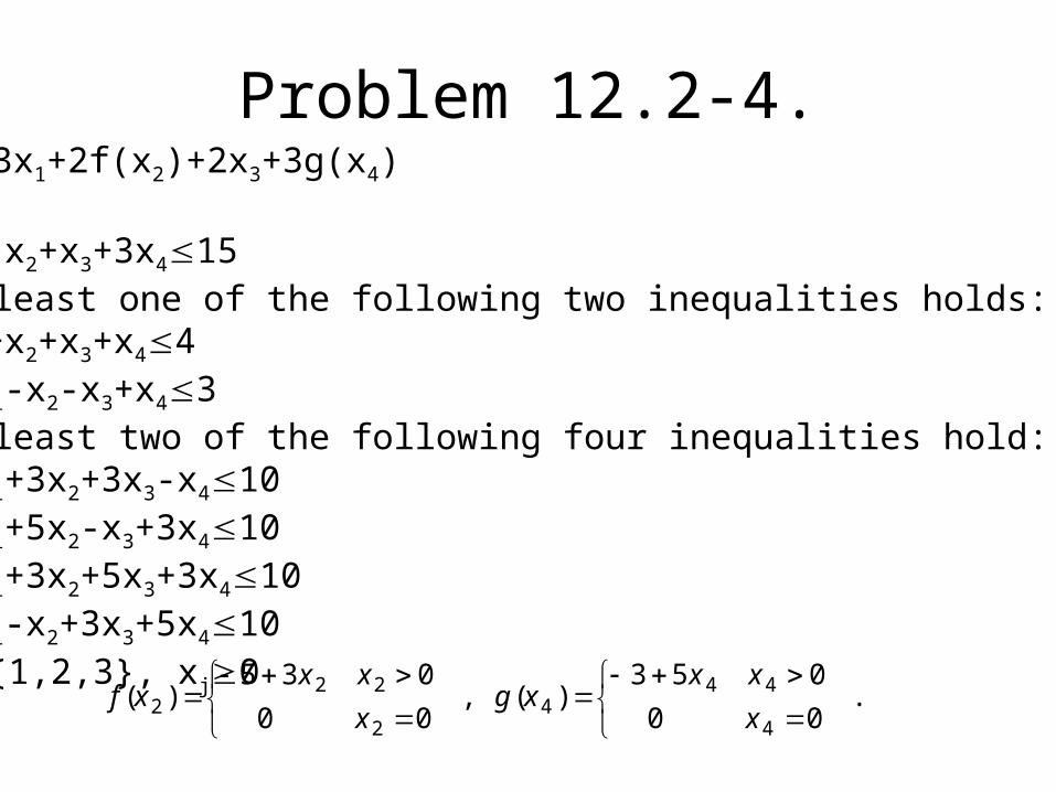
Problem 12.2-4.max Z=3x1+2f(x2)+2x3+3g(x4)s.t.1) 2x1-x2+x3+3x4152) At least one of the following two inequalities holds: x1+x2+x3+x44 3x1-x2-x3+x433) At least two of the following four inequalities hold: 5x1+3x2+3x3-x410 2x1+5x2-x3+3x410 -x1+3x2+5x3+3x410 3x1-x2+3x3+5x4104) x3{1,2,3}, xj05)

.)(,)(

00

053

00

035

4

444

2

222 x

xxxg

x

xxxf

Problem 12.3-4.

max Z=4x12-x1

3+10x22-x2

4

s.t.x1+x23x1,x20, x1,x2Z

Formulate a BIP model where the binary variables have the interpretation

Formulate a BIP model where the binary variables have the interpretation

jx

jxy

i

iij 0

1

jx

jxy

i

iij 0

1

Problem 12.4-1.

max Z=5x1+2x2

s.t.-x1+2x24 x1-x21 4x1+x212 x1,x20, x1,x2Z

a) Solve this problem graphicallyb) Solve the LP relaxation graphically, round the solution in all possible ways and check the solutions for feasibility and opti- mality.

Problem 12.7-1.

For each of the following constraints of pure BIP problems, usethe constraint to fix as many variables as possible:

a) 4x1+x2+3x3+2x42

b) 4x1-x2+3x3+2x42

c) 4x1-x2+3x3+2x47

Problem 12.7-3.

Use the following set of constraints for the same pure BIP problemto fix as many variables as possible. Also identify the constraintswhich become redundant because of the fixed variables.

3x3-x5+x71x2+x4+x6 1x1-2x5+2x62x1+x2-x40

Problem 12.7-10.

One of the constraints of a certain pure BIP problem is

3x1+4x2+2x3+5x47

Identify all the minimal covers for this constraint, and then givethe corresponding cutting planes.

Network Analysis

• Prototype Example

• Terminology

• Shortest-Path Problem

• Minimum-Spanning-Tree Problem

• Maximum-Flow Problem

Prototype Example

Shortest-Path Problem• Objective of the nth iteration: Find the nth nearest node to the origin

(repeat until n is destination)• Input for nth iteration: n-1 nearest nodes to the origin (solved for at

prev. Iterations), including their shortest path and distance to the origin• Candidates for nth nearest node: Each solved node that is directly

connected to one or more unsolved nodes provides a candidate - the unsolved node with the shortest connecting link

• Calculation of nth nearest node: For each solved node and the candidate, add the distance between them and the distance of the shortest path from the origin to this solved node. The candidate with the smallest sum is the nth nearest node, the shortest path is the one generating this distance.

Minimum Spanning Tree Problem

1 Select any node arbitrarily, then connect it (i.e., add a link) to the nearest distinct node

2 Identify the unconnected node that is closest to a connected node, and then connect these two nodes. Repeat this step until all nodes have been connected

3 Tie breaking: Ties for the nearest distinct node (step 1) or the closest unconnected node (step 2) may be broken arbitrarily, and the algorithm must still yield an optimal solution. However, such ties are a signal that there may be (but need not be) multiple optimal solutions. All such optimal solutions can be identified by pursuing all ways of breaking ties to their conclusion

Maximum-Flow Problem1 Identify an augmenting path by finding some directed path from

the supply node to the demand node in the residual network such that every arc on this path has strictly positive residual capacity (if no augmenting path exists, the net flows already assigned constitute an optimal flow pattern)

2 Identify the residual capacity c* of this augmenting path by finding the minimum of the residual capacities of the arcs on this path. Increase the flow in this path by c*

3 Decrease by c* the residual capacity of each arc on this augmenting path. Increase by c* the residual capacity of each arc in the opposite direction on this augmenting path. Return to step 1

Data Envelopment Analysis

• Description of the Method

• Example: Evaluating the Performance of Hospitals

• Example: Evaluating the Performance of Universities

• Some Important Aspects

Data Envelopment Analysis

– Purpose:

DEA can be used to measure the relative efficiency of units with the same goals and objectives.

– Applications:

Hospitals, banks, schools,...

– Algorithm:

Construction of a (hypothetical) „composite unit“ (weighted average of all units under consideration), comparison of input/output of each unit to be examined with the composite unit assessing the efficiency of each unit relative to the composite unit.

Example: Hospitals

• Data:

Hospital

Input Measure General University County State

# Personnel 285.2 162.3 275.7 210.4

Supply Exp. 123.8 128.7 348.5 154.1

Bed-days av. 106.72 64.21 104.1 104.04

Output Measure

Medicare patient days 48.14 34.62 36.72 33.16

Non-medicare pat. days 43.1 27.11 45.98 56.46

Nurses trained 253 148 175 160

Interns trained 41 27 23 84

Example: Hospitals

Components of the DEA model:

For each output measure:

Output of composite unit output of unit currently investigated

For each input measure:

Input of composite unit input of unit currently inv. * E

Objective function: min E

Interpretation: If a solution with E < 1 can be found, the unit investigated is relatively inefficient.

Example: Universities

There exist several slightly different formulations of DEA models. For the university example, the following model is used:

Inputs yjk: Budget (excl. personnel), Personnel budget, # students

Outputs xik: # graduates, # teaching hrs., # research projects, # publ.

ui,vj...weights for output and input factors

Basic model:

11110

s.t.

3

1

4

1

,,

max

ke

yv

xu

e

k

jjkj

iiki

k

Example: UniversitiesTo break the overall efficiency ek down into the components „research efficiency“ and „teaching efficiency“, the model is refined as follows:

Additional variables:

qj...proportion of input factor j associated with teaching

(1-qj)...proportion of input factor j associated with research

tk...relative teaching efficiency of university k

rk...relative research efficiency of university k

Additional constraints:

2

1

4

3

2

133

2

1

1j

jkjj

iiki

k

jkjkjj

iiki

k

yvq

xu

r

yvyvq

xu

t

)(

Some Important Aspects

• E < 1 means „relatively inefficient“, E = 1 does not necessarily mean „relatively efficient“

• In case of a „super-unit“ (produces the most of every output while using the least of every input), all units but the super-unit are relatively inefficient

• In practical problems, roughly 50% of the operating units can be identified as inefficient

• Sensitivity analysis is possible and can yield important insights: Vary one input or output of an inefficient unit at a time to see which level of this factor would turn the unit efficient

Inventory Theory

• Examples

• Components of Inventory Models

• Deterministic Models

• Stochastic Models

Example 1: Manufacturing Speakers for TV Sets

A TV manufacturing company produces its own speakers. TV sets are assembled on a continuous production line at a rate of 8000 per month, with one speaker needed per set. Speakers are produced in batches and placed into inventory until they are needed for assembly into TV sets. The company is interested in deter-mining when to produce a batch of speakers and how many speakers to produce in each batch. Several costs must be considered:

1) Each time a batch is produced, a setup cost of 12000 is incurred. The existence of setup costs argues for producing speakers in large batches.

2) The unit production cost of a single speaker (excluding setup) is 10$, independent of the batch size produced.

3) The holding cost of keeping a speaker in stock is 0.3 per month. The existence of holding costs argues for producing small batches.

4) Each speaker not available when required leads to shortage costs of 1.10 per month.

Example 2: Wholesale Distribution of Bicycles

A wholesale distributor purchases bicycles from the manufacturer monthly and supplies them to various shops in response to purchase orders. The total demand from bicycle shops in a given month is uncertain. The wholesale distributor faces the problem of how many bicycles to order from the manufacturer for any given month, given the stock level leading into that month.

The following costs have been determined to be important:

1) The ordering cost (fixed cost of $200 per order plus variable cost of $35 per bicycle)

2) The holding cost (= cost of maintaining an inventory, $1 per bicycle and month)

3) The shortage cost (= cost of not having a bicycle on hand when needed), estimated at $15 per bicycle. Included in this cost is loss of goodwill, cost

of delay in revenue received,...

Lesson

Inventory models and production planning models are closely related.

Components of Inventory Models

• Cost of ordering/manufacturing z units: c(z)– e.g. c(z)=K+cz (linear cost function)

• Holding cost

• Shortage cost („unsatisfied demand cost“)

• Backlogging: excess demand is not lost, but satisfied later using the next normal delivery

• No backlogging: excess demand can only be satisfied by a priority shipment and is lost otherwise

Components of Inventory Models

• Revenue may or may not be included in the model. However, if revenue is neglected, the loss in revenue must be included into the shortage cost.

• Salvage value stands for the value of items left over when no inventory is needed anymore.

• The discount rate is used to take into account the time value of money (holding cost through capital tied up in inventory).

The Standard EOQ Model

Assumptions:– Inventory is depleted at a constant rate a

– Inventory is replenished by immediate arrival of Q ordered units at the desired time

Costs to be considered:

– K...setup cost for producing or ordering one batch

– c...unit cost for producing or purchasing one unit

– h...holding cost per unit and unit of time held in inventory

?: When and by how much should the inventory be replenished so as to minimize the sum of these costs per unit of time.

The Standard EOQ Model

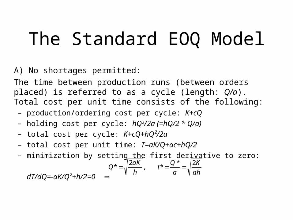
A) No shortages permitted:

The time between production runs (between orders placed) is referred to as a cycle (length: Q/a). Total cost per unit time consists of the following:– production/ordering cost per cycle: K+cQ

– holding cost per cycle: hQ2/2a (=hQ/2 * Q/a)

– total cost per cycle: K+cQ+hQ²/2a

– total cost per unit time: T=aK/Q+ac+hQ/2

– minimization by setting the first derivative to zero:

dT/dQ=-aK/Q²+h/2=0 ah

K

a

Qt

h

aKQ

22

**,*

The Standard EOQ ModelB) Shortages permitted:

Shortages are allowed, but incur a cost of

p...shortage cost per unit and unit of time short,

S...inventory level just after adding a batch of Q units,

Q-S...shortage just before a batch of Q units is added.

To determine the total costs, note that ordering costs per cycle do not change!– Holding cost per cycle: hS/2*S/a=hS²/2a (inventory only positive for a time S/a!)

– shortage cost per cycle: p(Q-S)/2*(Q-S)/a=p(Q-S)²/2a

– total cost per cycle: K+cQ+hS²/2a+p(Q-S)²/2a

– total cost per unit time: T=aK/Q+ac+hS²/2Q+p(Q-S)²/2Q.

The model has 2 decision variables (S and Q), so minimization requires setting the partial derivatives to 0.

The Standard EOQ ModelB) (continued)

Solving these equations simultaneously leads to

Optimal cycle length:

022

0

2

2

2

2

2

Q

SQp

Q

SQp

Q

hS

Q

aK

Q

T

Q

SQp

Q

hS

S

T

)()(

)(

.*,*p

hp

h

aKQ

hp

p

h

aKS

22

p

hp

ah

K

a

Qt

2**

The Standard EOQ ModelC) Quantity discounts, no shortages permitted:

If quantity discounts are introduced into the standard EOQ model, the standard procedure is to find the minimum for each of the resulting cost curves, compare the total cost per unit time, and choose the minimum.

Stochastic Models

A) Single period, no setup cost:

„Bicycle Example“, Assumptions: – no reorders possible (production of bicycle discontinued,...)– no setup cost for wholesaler– holding cost + salvage value = $9– selling price = $45, profit per bicycle = $25– no goodwill lost in case of unsatisfied demand

D...demand by bicycle shops (random variable),

y...number of bicycles purchased by distributor

Net income = 45 min{D,y} - 20y + 9 max{0,y-D}=

= 45D - 45 max{0,D-y} - 20y + 9 max{0,y-D}

Stochastic Models

A) Single period, no setup cost (continued)

Objective: minimize expected total cost

Probability distribution of D is needed to determine an optimal policy:

PD(d)=P{D=d} is known for all values of d

Summary:– Planning is done for just a single period.

– The demand D is a random variable with a known probability distribution.

– There is no initial inventory at hand.

– The only decision variable is y, the number of units to purchase or produce for inventory at the beginning of the period.

– The objective is to minimize the expected total cost.

Stochastic Models

The discrete random variable D is often approximated by a continuous random variable for simplicity of solution.

yd

y

dDD

dD

dPdyhdPydpcy

dPdyhydpcyyDCEyC

DyhyDpcyyDC

1

0

0

00

:function obj.

00

)()()()(

)(}),max{},max{()],([)(min

},max{},max{),(

a

0

D D) of fct. distr. cum. the (i.e.,(a)

D, of fct.density prob.

d

D

)(

)(

Stochastic Models

Expected cost then becomes

hp

cpyyy

yLcy

dyhdypcy

dyhypcy

dyCyDCEyC

D

y

y

D

D

D

)(|

)(

)()()()(

)(}),max{},max{(

)(),()],([)(

00

0

0

0

00

LINGO

• Basic features of the LINGO modelling language

• Basic LINGO syntax

• Sets and derived sets

• Example models

Basic Features

Lingo is a specification language - you tell it what you want, not how to do it!

Lingo can solve

• direct models,

• simultaneous models,

• optimization models,

where models may be linear or non-linear, continuous or integer.

Basic LINGO Syntax

• Order of statements is unimportant

• Lingo is not case-sensitive, y=Y

• Statements must be terminated by a semicolon (;)

x=3y+2z ;

• Comments begin with an exclamation point (!) and end with a semicolon (;)

! This is a comment ;

Variable Types

• The default variable type is a continuous variable that is restricted to the range (0,).

• To restrict a variable X to integer values, the statement @GIN(X) is used.

• To restrict a variable X to be binary, the statement @BIN(X) is used.

• To allow any negative or positive value for a variable X, the statement @FREE(X) is used.

• To set a different variable range, use the statement @BND(lower_bound, X, upper_bound).

Model Types

• Direct Models

• Simultaneous Models

• Optimization Models

The SETS section of a model

• Primitive Sets vs. Derived Sets (covered later)

• Set Syntax:

name / members / : attributes;

• Example:

SETS:

Students / John, Jill, Mike, Mary/ : sex, age;

ENDSETS

The DATA section of a model

• Syntax: attribute = value_list;

• Example:

DATA:

Age = 20 19 18 21;

Sex = 0,1,0,1;

ENDDATA

Accessing Set Elements: @FOR• @FOR is one of the set looping functions provided by LINGO• Syntax:

@FOR(set (set_index_list) | conditional_qualifier :expression);

(the set_index_list is optional)• Example:

SETS:

Number / 1..5/ :X;

ENDSETS

@FOR(Number(i): X(i)=i-1);

END

Indices are automatically maintained by LINGO and begin with 1.

@FOR with conditional qualifiers

• Sample model: RECIP.LNG

Logical Operators

• #NOT#, #EQ#, #NE#, #GT#, #GE#, #LT#, #LE#, #AND#, #OR#

• Important: Distinguish between these logical operators and =, < and >!

• < is the same as , > is the same as !

• @IN(element, set) is true if the set contains the element

• @SIZE(set) returns the no. of elements in the set.

Other Set-Looping Functions

• @SUM(set_name : expression)

Example: MIN=@SUM(...)

• @MIN(set_name : expression)

• @MAX(set_name : expression)

Derived Sets• A derived set is a set derived from primitive sets.• Dense derived sets:

Syntax: set_name (parent_sets) [: attributes];

Example: ROUTES(WAREHOUSE, CUSTOMER) : COST;• Sparse derived set (explicit):

Syntax: set_name (parent_sets) / explicit_list /[: attributes];

Example: PLPR(PLANT,PROD) / A,X A,Y B,Y / : UNITCOST;• Sparse derived sets (with membership conditions):

Syntax: set_name (parent_sets) | condition [: attributes];

Example: PAIR(OBJ,OBJ) | &1 #LT# &2 : C,X;• Example Models: TRAN.LNG, PERT.LNG, MATCH.LNG