....

Mathematical modelingof free-flooding anti-rolltanks

M.A. van Slooten

.

Mas

ter’s

thes

is

....

Mathematical modeling offree-flooding anti-roll tanks

by

M.A. van Slooten

in partial fulfillment of the requirements for the degree of

Master of Sciencein Marine Technology - Specialisation Ship Hydromechanics

at the Delft University of Technology,to be defended publicly on Friday April 11, 2014 at 14:00 AM.

Student number: 1283588Supervisor: Prof. dr. ir. R. H. M. HuijsmansThesis committee: Ir. K. van den Berg, Vuyk Engineering Rotterdam

Ir. N. Carette, MARINDr. ir. J. A. Keuning, TU DelftIr. K. Visser SBN-b.d., TU Delft

An electronic version of this thesis is available at http://repository.tudelft.nl/.

Preface

The thesis project presented in this report has been carried out at Vuyk Engineering Rotterdam.It highlights an understudied topic in the category anti-rolling devices: themodeling of free-floodinganti-roll tanks. As these type of anti-roll devices have only sporadically been considered andapplied over the past century, their modeling has hardly been addressed. The findings on themost current mathematical model available are presented here.

I would like to thank my supervisors at Vuyk Engineering Rotterdam, ir. Kuno van den Berg,and at Delft University of Technology, prof. dr. ir. R.H.M. Huijsmans in helping me decipheringall the different components and influences on themathematical model presented in this report.In that context I must also include ir. Nicolas Carette for his insights into essential conditionsfor successful simulation of the problem at hand. Besides themembers of my thesis committeemy special thanks goes out to Elena Stroo-Moredo MSc, who agreed to be my mentor for thisproject and has taken the trouble to review every scrap of text I have produced. And lastly,the following people have been very important to me: my colleagues at Vuyk EngineeringRotterdam, to whom I could always turn with questions, and of course to all my friends andfamily, who have supported me throughout my studies.

M.A. van SlootenDelft, March 2014

iii

Contents

List of Figures vii

List of Tables ix

1 Introduction 11.1 Background . . . . . . . . . . . . . . . . . . . . . . . . . . . . . . . . . . . . . . . . . 11.2 Why free-flooding tanks . . . . . . . . . . . . . . . . . . . . . . . . . . . . . . . . . 21.3 Aims. . . . . . . . . . . . . . . . . . . . . . . . . . . . . . . . . . . . . . . . . . . . . . 41.4 Programs. . . . . . . . . . . . . . . . . . . . . . . . . . . . . . . . . . . . . . . . . . . 41.5 Outline . . . . . . . . . . . . . . . . . . . . . . . . . . . . . . . . . . . . . . . . . . . . 5

2 Literature review 72.1 History . . . . . . . . . . . . . . . . . . . . . . . . . . . . . . . . . . . . . . . . . . . . 72.2 Characteristics free-flooding anti-roll tank . . . . . . . . . . . . . . . . . . . . . 92.3 Mathematical modeling . . . . . . . . . . . . . . . . . . . . . . . . . . . . . . . . . 102.4 Conclusion . . . . . . . . . . . . . . . . . . . . . . . . . . . . . . . . . . . . . . . . . 132.5 Bibliography literature . . . . . . . . . . . . . . . . . . . . . . . . . . . . . . . . . . 14

3 Theory 173.1 Introduction. . . . . . . . . . . . . . . . . . . . . . . . . . . . . . . . . . . . . . . . . 173.2 Mathematical model of tank . . . . . . . . . . . . . . . . . . . . . . . . . . . . . . 18

3.2.1 Dynamic water pressure . . . . . . . . . . . . . . . . . . . . . . . . . . . . 233.2.2 Dynamic air pressure . . . . . . . . . . . . . . . . . . . . . . . . . . . . . . 263.2.3 Unknown parameters . . . . . . . . . . . . . . . . . . . . . . . . . . . . . . 29

3.3 Time domain . . . . . . . . . . . . . . . . . . . . . . . . . . . . . . . . . . . . . . . . 313.3.1 Properties of the non-linear system . . . . . . . . . . . . . . . . . . . . . 323.3.2 Solving the system . . . . . . . . . . . . . . . . . . . . . . . . . . . . . . . . 353.3.3 Coupling with ship motions . . . . . . . . . . . . . . . . . . . . . . . . . . 38

3.4 Frequency domain . . . . . . . . . . . . . . . . . . . . . . . . . . . . . . . . . . . . 403.4.1 Coupling with ship motions . . . . . . . . . . . . . . . . . . . . . . . . . . 42

4 Results 454.1 Time domain . . . . . . . . . . . . . . . . . . . . . . . . . . . . . . . . . . . . . . . . 49

4.1.1 indirect AQWA-NAUT simulation. . . . . . . . . . . . . . . . . . . . . . . 51

v

vi Contents

4.1.2 direct AQWA-NAUT simulation . . . . . . . . . . . . . . . . . . . . . . . . 554.1.3 SCILAB simulation . . . . . . . . . . . . . . . . . . . . . . . . . . . . . . . . 57

4.2 Frequency domain . . . . . . . . . . . . . . . . . . . . . . . . . . . . . . . . . . . . 594.2.1 Regular wave response . . . . . . . . . . . . . . . . . . . . . . . . . . . . . 594.2.2 Irregular wave response . . . . . . . . . . . . . . . . . . . . . . . . . . . . 61

4.3 Discussion of results . . . . . . . . . . . . . . . . . . . . . . . . . . . . . . . . . . . 634.3.1 Linearization of model . . . . . . . . . . . . . . . . . . . . . . . . . . . . . . 634.3.2 Comparison of simulation types . . . . . . . . . . . . . . . . . . . . . . . 634.3.3 Comparison of Webster Model with VER Model . . . . . . . . . . . . . 644.3.4 Comparison of air configurations . . . . . . . . . . . . . . . . . . . . . . 654.3.5 Influence of radiation pressure . . . . . . . . . . . . . . . . . . . . . . . . 664.3.6 Influence of tank parameters on tank performance . . . . . . . . . . . 67

5 Conclusions and recommendations 735.1 Conclusions. . . . . . . . . . . . . . . . . . . . . . . . . . . . . . . . . . . . . . . . . 735.2 Recommendations. . . . . . . . . . . . . . . . . . . . . . . . . . . . . . . . . . . . . 74

Bibliography 74

A Dynamic air pressure 77

B Numerical methods 81B.1 Fixed step method (Runge-Kutta) . . . . . . . . . . . . . . . . . . . . . . . . . . . 81B.2 Variable step method (Cash-Karp) . . . . . . . . . . . . . . . . . . . . . . . . . . 82

C Theory of decay analysis 85

D RAOs for all motion directions 89

List of Figures

1.1 External free-flooding anti-roll tanks in the form of sponsons . . . . . . . . . . . 21.2 Internal free-flooding tanks . . . . . . . . . . . . . . . . . . . . . . . . . . . . . 31.3 Types of anti-roll tanks . . . . . . . . . . . . . . . . . . . . . . . . . . . . . . . . 3

2.1 Free-flooding anti-roll tanks on the Deutschland [5] . . . . . . . . . . . . . . . . 82.2 Free-flooding anti-roll tanks fitted on the Pensacola and Northampton classes 82.3 Possible locations and shapes of flooding ports . . . . . . . . . . . . . . . . . 102.4 Active anti-roll tank . . . . . . . . . . . . . . . . . . . . . . . . . . . . . . . . . 10

3.1 Ship axes convention . . . . . . . . . . . . . . . . . . . . . . . . . . . . . . . . 173.2 Isolated tank [9] . . . . . . . . . . . . . . . . . . . . . . . . . . . . . . . . . . . . 183.3 Flow rate equality . . . . . . . . . . . . . . . . . . . . . . . . . . . . . . . . . . . 203.4 Pressure head components . . . . . . . . . . . . . . . . . . . . . . . . . . . . . 213.5 Water level dependence on excitation frequency, fully vented tanks . . . . . . . 253.6 Roll period for cancellation point versus forced roll angle amplitude . . . . . . . 263.7 Passive air configurations . . . . . . . . . . . . . . . . . . . . . . . . . . . . . . 273.8 Free-flooding anti-roll tank as designed for USS Midway [9] . . . . . . . . . . . 313.9 Equilibrium point analysis non-linear equation . . . . . . . . . . . . . . . . . . . 333.10 Global error for the Modified Euler method . . . . . . . . . . . . . . . . . . . . 353.11 Computation time and error of fixed step methods (visibly smooth and matching

the exact solution) . . . . . . . . . . . . . . . . . . . . . . . . . . . . . . . . . . 363.12 Instability of the Runge-Kutta-Fehlberg method . . . . . . . . . . . . . . . . . . 373.13 Computation time and error of variable stepmethods (visibly smooth andmatching

the exact solution) . . . . . . . . . . . . . . . . . . . . . . . . . . . . . . . . . . 373.14 Change in water level in the time domain including acceleration terms . . . . . 403.15 Change in water level in the time domain excluding acceleration terms . . . . 41

4.1 RAOs of roll with and without viscous damping . . . . . . . . . . . . . . . . . . 474.2 Influence of loss of buoyancy on the metacentric height . . . . . . . . . . . . . 494.3 Non-physical result SCILAB . . . . . . . . . . . . . . . . . . . . . . . . . . . . 514.4 Non-physical result AQWA-NAUT . . . . . . . . . . . . . . . . . . . . . . . . . . 514.5 Free decay test . . . . . . . . . . . . . . . . . . . . . . . . . . . . . . . . . . . . 534.6 Trade-off between accuracy and computing time (free decay test) . . . . . . . . 54

vii

viii List of Figures

4.7 Time simulation of equivalent damping (AQWA-NAUT) . . . . . . . . . . . . . . 544.8 Motion of the ship and tank water levels (AQWA-NAUT) . . . . . . . . . . . . . 564.9 Wave potential damping on roll motion . . . . . . . . . . . . . . . . . . . . . . . 574.10 Time simulation tuned tank (SCILAB) . . . . . . . . . . . . . . . . . . . . . . . . 584.11 Trade off between accuracy and computing time (wave excited simulation) . . 584.12 RAOs for roll with the tuned tank in a regular wave . . . . . . . . . . . . . . . . 604.13 Overdamped RAOs for roll with the tuned tank in a regular wave (0.17𝐶 ) . . . 614.14 RAOs for roll with the tuned tank in an irregular wave spectrum . . . . . . . . . 624.15 Tank performance for different wave heights . . . . . . . . . . . . . . . . . . . . 634.16 Comparison of time and frequency domain simulation results . . . . . . . . . . 644.17 The tanks used for comparison of modeling . . . . . . . . . . . . . . . . . . . . 644.18 Comparison of frequency domain results for different air configurations . . . . . 664.19 Influence of pressure head components on tank performance . . . . . . . . . . 664.20 Influence of 𝑑 and 𝛾 on the tank transfer period . . . . . . . . . . . . . . . . . 674.21 Tank moment amplitude and phase . . . . . . . . . . . . . . . . . . . . . . . . . 684.22 Influence of tank transfer period on tank performance . . . . . . . . . . . . . . 684.23 Influence of free surface area on tank performance . . . . . . . . . . . . . . . . 694.24 Influence of flooding port size on performance . . . . . . . . . . . . . . . . . . . 704.25 Influence of flooding port discharge coefficient on water level . . . . . . . . . . 704.26 Influence of air coefficients on tank performance . . . . . . . . . . . . . . . . . 714.27 Influence of combined air vent coefficients 𝛼𝐶 on tank performance . . . . . 71

D.1 RAOs for surge with the tuned tank in a regular wave . . . . . . . . . . . . . . 90D.2 RAOs for sway with the tuned tank in a regular wave . . . . . . . . . . . . . . . 91D.3 RAOs for heave with the tuned tank in a regular wave . . . . . . . . . . . . . . 92D.4 RAOs for roll with the tuned tank in a regular wave . . . . . . . . . . . . . . . . 93D.5 RAOs for pitch with the tuned tank in a regular wave . . . . . . . . . . . . . . . 94D.6 RAOs for yaw with the tuned tank in a regular wave . . . . . . . . . . . . . . . 95

List of Tables

1.1 Types of anti-roll systems [3] . . . . . . . . . . . . . . . . . . . . . . . . . . . . 2

2.1 Working principles of fluid anti-roll systems . . . . . . . . . . . . . . . . . . . . 12

3.1 Calculation parameters . . . . . . . . . . . . . . . . . . . . . . . . . . . . . . . 243.2 Passive air configurations . . . . . . . . . . . . . . . . . . . . . . . . . . . . . . 273.3 Overview of the air constants . . . . . . . . . . . . . . . . . . . . . . . . . . . . 29

4.1 Ship particulars and loading condition . . . . . . . . . . . . . . . . . . . . . . . 464.2 Particulars for isolated free-flooding tank . . . . . . . . . . . . . . . . . . . . . . 484.3 Non-dimensional damping coefficient . . . . . . . . . . . . . . . . . . . . . . . . 57

ix

Nomenclature

𝛼 ration of vent or crossover area totank free surface area

𝛽 ratio of flooding port area to tankfree surface area

Δ𝐻( ) complex amplitude of differentialpressure head across one floodingport

𝛾 nondimensional half U-tube length

𝜔 wave frequency

𝐺𝑀 transverse metacentric height

𝑈 complex air pressure couplingconstant

𝑉( ) complex air pressure constant (onone side)

Φ diffraction potential

Φ incident wave potential

Φ radiation potential, 𝑚-th mode

Υ( ) tank water motion (on one side)

Υ tank water level on the oppositeside

𝜉 complex ship motion amplitude,𝑚-th mode

𝜁 regular wave amplitude

𝐴(𝑠) cross-sectional area of tank atpoint 𝑠 on the streamline

𝐴 area of free surface in tank

𝐶 dynamic arm of tank moment

𝐶 coupling coefficient of tank intoship motion

𝐶 effective discharge coefficient forair vent or crossover

𝐶 critical linear tank dampingcoefficient

𝐶 effective discharge coefficientflooding port

𝑑 distance between flooding portand equilibrium tank water level

𝑑 distance between flooding portand still-water line

𝐺 complex coefficient of tanktransfer function on one side

𝐻 dynamic water pressure head

𝑙 /𝑏 length/width of tank

𝑝 equilibrium air pressure in tank

𝑝 dynamic air pressure in tank

𝑝 atmospheric pressure

𝑅 equilibrium pressure in head ofwater

𝑅 dimensional constant for dynamicair pressure analysis

xi

xii List of Tables

𝑅 linearized discharge coefficient aircrossover

𝑠 streamline coordinate

𝑇 natural period of roll

𝑇 tank transfer period

𝑣 instantaneous vertical velocityalong the streamline

𝑥 longitudinal location of centroidof equilibrium tank free-surface,

positive to bow

𝑦 lateral location of centroid ofequilibrium tank free-surface,positive to port

𝑍 motion of isolated tank

𝑧 , wave elevation at the flooding porton one side

DoF Degrees of Freedom

1Introduction

1.1. BackgroundA growing area in the offshore industry is the development of offshore wind farms. As thedemand for clean energy has increased, so did interest in creating energy using wind turbines.Better wind speeds are available offshore compared to on land and complaints from localresidents about visual pollution are largely diminished. A high degree of precision is neededto assemble the wind turbine components. It is impossible to position a component in the rightplace if the ship experiences significant motions. As the offloading of wind turbine componentsprogresses themetacentric height of the ship varies greatly, in turn influencing the shipmotions.A way to minimize ship motions in all the loading conditions is attractive as it will extend theoperational window of the offshore installation vessel.

A notorious movement for interruption of operations is the roll motion of the ship, whichcan become very large at resonance frequency, thus the focus for motion reducing methodsis usually on reducing the roll motion specifically. The roll motion can be reduced by installinga device, which counteracts the heeling moment with an opposing moment. The possibilitiesfor such a device arranged by type of mass are listed in table 1.1. In recent years there is anincreasing interest in the application of free-flooding anti-roll tanks.

In 2009/2010 Vuyk Engineering Rotterdam (VER) performed an investigation into externalfree-flooding anti-roll tanks for the Sea Trucks Group in cooperation with MARIN. The additionof free-flooding anti-roll tanks in the form of sponsons to two existing pipelaying crane shipswas studied [1],[2]. In figure 1.1 the sponson is shown. A time domain mathematical modelfor pure roll (single degree of freedom and a dynamic water pressure based on the velocityhead) was developed in Excel with input of ship motions in the form of response amplitudeoperators (RAOs) from AQWA (3D diffraction program). This model is called the VER Modelfrom here on. The decrease in roll motion was estimated to be about 37% for free-floodingtanks with a capacity of 2.75% of the ship’s displacement.

For verification of the results the same ship and lay-out of the free-flooding anti-roll tanks

1

2 1. Introduction

SOLID FLUIDwheel fins or ruddergyroscope doughnut tankunbalanced wheel U-tube tankspendulum free-surface tanksrolling ball free-flooding tanks

Table 1.1: Types of anti-roll systems [3]

Figure 1.1: External free-flooding anti-roll tanks in the form of sponsons

was revisited at the Maritime Research Institute Netherlands (MARIN) [4],[5]. This study wasconducted in Fredyn (3D diffraction) and ReFRESCO (Computational Fluid Dynamics - CFD).Their conclusion was that the damping was well predicted by the VER Model, but that in theirmodel the initial transverse stability (𝐺𝑀 -value) was significantly altered by the addition ofthe anti-roll tanks on the outside of the ship. According to the study the anti-roll tanks onlycompensate the unfavorable change of stability by the addition of the tanks and do not improvethe stability of the ship in the original situation.

On account of these studies the customer was advised not to mount sponsons on thepipelaying vessels, since the investment would be disproportionate to the expected dampingof the rolling motion. This result was disappointing, especially in the light that experimentssuggest that free-flooding anti-roll tanks are effective roll dampers. It is thought that internaltanks will give better results than external tanks. In figure 1.2 an application of an internalfree-flooding anti-roll tank is shown.

1.2. Why free-flooding tanksOne way of stabilizing a ship is by anti-roll tanks. There are three kinds of anti-roll tanks,shown in figure 1.3: the free-surface, U-tube and free-flooding tanks. A free-flooding tank is

1.2. Why free-flooding tanks 3

Figure 1.2: Internal free-flooding tanks

considered to resemble a U-tube tank, but with an external crossover duct instead of an internalcrossover duct. Of these the free-flooding anti-roll tank is the least known and applied. Thereason is that the performance of these tanks is reduced due to a momentum drag penaltyincurred at forward speeds. However, at low forward speeds this drag penalty is negligible. Ifdesirable, the tanks could be closed off and emptied for transit.

(a) free-surface tank (b) U-tube tank (c) free-flooding tank

Figure 1.3: Types of anti-roll tanks

The reason for choosing anti-roll tanks as a stabilization device for a vessel is, amongothers, the relatively low cost of building the system and the fact that they continue to workwhen the vessel is stationary, in contrast to fin-type anti-rolling devices (save for active finstabilizers). The second is interesting for offshore vessels, which remain stationary or sail atvery low speeds in operation. Also, when using free-flooding tanks in operation, themomentumdrag penalty incurred at higher forward speeds is avoided. Active fin stabilizers have beenheavily developed in recent years and are now more effective at zero speed, but are a lotmore expensive than anti-roll tanks.

Offshore installation vessels generally have a broad beam, which is necessary to haveenough deck space for the storage of the installation components and generate enough buoyancyand stability during for instance lifting. As the components on board are installed the loadingcondition of the vessel changes: the vessel sits higher in the water and the metacentric heightincreases. The metacentric height is inversely related to the roll period, so as the first rises the

4 1. Introduction

second decreases and the natural rolling period comes closer to the range of most commonlyfound waves. When the wave period is close to the natural rolling period the ship motionsare the largest, which is detrimental to the operation. The 𝐺𝑀 is generally lowered againby adding water ballast as the operation progresses. To further minimize roll motions duringoperations anti-roll tanks can be used.

The center part of the vessel is generally occupied bymachinery and installation components.U-tube tanks and free-surface tanks both require a considerable amount of space in the centerpart of the vessel to accommodate the crossover connection. Free-flooding anti-roll tanks donot require a considerable amount of space in the center part of the vessel, but can be builtinto the sides where, in the case of offshore installation vessels, due to the broad beam plentyof space is available. This makes free-flooding tanks the most suitable for retrofitting existingships. Of course, free-flooding tanks also have disadvantages. These are highlighted in § 2.2.

1.3. AimsThe basis for this graduation project is the modeling of internal free-flooding anti-roll tanks,with as intended result a suitable method or application for use at VER. The goal of thisthesis is, therefore, not to develop a complete new theory for predicting the performance ofa free-flooding tank, but to find the most suitable analytical mathematical model and developthe practical application in which this theory is applied.

1.4. ProgramsAQWA ANSYS AQWA software is an engineering analysis suite of tools for the investigationof the effects of wave, wind and current on floating and fixed offshore and marine structures.This software package is well recognized in the offshore andmarine industry. The RAOs in thisreport are calculated using the 3D diffraction software AQWA-LINE [6] and the time domainsimulations are performed using AQWA-NAUT [7].

[AQWA-LINE] can simulate linearized hydrodynamic fluid wave loading on floatingor fixed rigid bodies. This is accomplished by employing three-dimensional radiation/diffractiontheory and/or Morison’s equation in regular waves in the frequency domain.

The real-time motion of a floating body or bodies while operating in regular waves[or irregular waves] can be simulatedwith [AQWA-NAUT], in which nonlinear Froude-Krylovand hydrostatic forces are estimated under instantaneous incident wave surface.External forces can be applied to the bodies at each time step imported or definedby a user-written dynamic-link library. The convolution approach is used to accountfor the memory effect of the radiation force. […] The program requires a fullhydrostatic and hydrodynamic description of each structure. This can be transferreddirectly from a backing file created as a result of an AQWA-LINE analysis.

1.5. Outline 5

SCILAB

SCILAB [8] is an open source, cross-platform numerical computational packageand a high-level, numerically oriented programming language. It can be used forsignal processing, statistical analysis, image enhancement, fluid dynamics simulations,numerical optimization, and modeling, simulation of explicit and implicit dynamicalsystems and (if the corresponding toolbox is installed) symbolic manipulations.SCILAB is the most complete open source alternative to MATLAB.

The language provides an interpreted programming environment, with matricesas the main data type. By using matrix-based computation, dynamic typing, andautomatic memory management, many numerical problems may be expressed ina reduced number of code lines, as compared to similar solutions using traditionallanguages, such as Fortran, C, or C++.

1.5. OutlineFirst, publicly available information is explored and assessed in the literature review, chapter 2.Based on the findings in this chapter the most appropriate mathematical model is chosen. Themotivation behind this model and its parts is elaborated upon in the chapter on the underlyingtheory of the model (chapter 3). The problem, as set forth in this chapter, is solved both inthe time domain and the frequency domain. The way of solving the problem in both domainsis part two of the chapter on theory. The results from the simulations in the time domainand the frequency domain are given in chapter 4. No experiments were performed to actuallyquantify the outcomes due to time restrictions, so themodel is only evaluated upon its accuracyas a mathematical model. Some restrictions to its application are explored here. Finally, inchapter 5, conclusions and recommendations are drawn on the effectiveness of free-floodingtanks and how to improve the results in this report.

2Literature review

2.1. HistoryMuch has been written about roll and roll stabilization. The term ’roll stabilization’ is in facta misnomer according to Goodrich [2.1], since all ships operating under normal conditionsare inherently stable. A device fitted to a ship to reduce the roll should be called a ’rolldamper’. However, the term roll stabilization has persisted and is commonly used in theliterature concerning roll reduction.

All ships in waves encounter roll motions, but before the industrial revolution roll motionswere not considered a problem and therefore did not constitute an important part in shipresearch. The reason for this is that sails damp the roll motions of the ship, which was theprimary means of powering ships in the Age of Sail. At the end of the 19th century motorizedvessels started replacing sail driven vessels and due to the differing transverse stability theseregularly experienced excessive roll motions.

Froude [2.2] was the first to describe this problem mathematically. He argued that rollmotion is a consequence of fluid pressure acting on the hull and not of the impact of waveson the side of the ship, which is a view still held today. The first ship to employ an anti-rolltank (free-surface) was the HMS Inflexible. The results of this full scale experiment has beenreported by Watts [2.3, 4]. The success was ambiguous: on the one hand the roll motion ofthe ship was significantly reduced in the resonance region, on the other hand a loss of stabilitywas found outside the resonance region due to the free-surface effect. The free-flooding tanks,which he called sea-ducted tanks, were conceived by Frahm [2.6] in 1911 and he planned toevaluate this concept in future research. Unfortunately, no record of this research can befound. In the 1930’s these free-flooding tanks were built into several passenger ferries inGermany (figure 2.1, see Hort [2.7] and Feld [2.8]). There is scant data on the performanceof the anti-roll tanks, because passengers insisted that the anti-roll tanks remain in service fortheir comfort.

7

8 2. Literature review

Figure 2.1: Free-flooding anti-roll tanks on the Deutschland [2.5]

Around the same time (1931) free-flooding tanks were retrofitted to 6 US Navy cruisers ofthe Pensacola and Northampton classes, see figure 2.2. These ships were known for theircruel behavior in rough seas. The free-flooding tanks installed on these war ships did nothave an air cross connection constructed between the port and starboard tanks due to spacerestrictions, thus differing from the original Frahm tanks. Despite initial misgivings the tankswere successful in reducing the roll motion by 30-40% and increasing the roll period by 20%.Unfortunately, even though it is the best documented application of free-flooding tanks, thereis not a lot of measured data on these installations as experiments were suspended due tothe outbreak of World War II.

Figure 2.2: Free-flooding anti-roll tanks fitted on the Pensacola and Northampton classes

Even though the free-flooding anti-roll tanks were effective, the system fell into generaldisuse after these applications. According to Webster et al. [2.9] this is probably due to thereduction in effectiveness under the operating conditions of most ships and the amount ofmaintenance that the tanks require.

2.2. Characteristics free-flooding anti-roll tank 9

For the next decades not a lot of research is done into free-flooding anti-roll tanks, but onlyinto free-surface and U-tube tanks. At the end of the eighties interest is rekindled for offshoreapplication. No records could be found of actual instances, but variations of free-floodinganti-roll tanks were developed and installed. The best known commercial development fromthis period is the Slo-Rol system by SEATEK Corporation.

The US Navy also renews its interest in free-flooding anti-roll tanks at this time, becauseretrofitting such a device (without a crossover duct) in an existing (war) ship was the onlyfeasible option. Webster et al. [2.9] concluded that properly designed free-flooding anti-rolltanks can achieve a useful amount of roll stabilization, but that the added resistance penaltythey generate could make such systems unattractive for higher ship operating speeds. Thefree-flooding tanks were never fitted to the object of study (the USN Midway), even though thestudy did show a possible reduction of the roll motion with 48%.

2.2. Characteristics free-flooding anti-roll tankThe above-mentioned momentum drag is proportional to the ship speed squared and makesthe free-flooding anti-roll tank increasingly unattractive with increasing speed. Mostly theyare applied in situations where the floating object is stationary. There are also some otherdisadvantages to free-flooding anti-roll tanks besides the drag penalty, such as highmaintenancelevel due to corrosion of the tank wall by the seawater. On the other hand, anti-roll tanksin general are appreciated for their simplicity, low cost, adaptability to temporary use (closeflooding ports or vents) and precisely because they still damp the roll motion at low or evenzero speed (Vasta et al [2.10]). Moaleji and Greig [2.11] submit that free-flooding anti-roll tanksare ideally suited for multi-hulls, because their side hulls are well separated providing a largelever arm and subsequently less water is required to achieve a given moment.

Possible locations on the hull of the flooding ports of the free-flooding anti-roll tanks, visualizedin figure 2.3, are in the bottom of the hull or in the side. If the flooding ports are located in theside of the hull around the water line ventilation can occur for large roll angles.

In contrast to free-surface tanks the free-flooding anti-roll tanks cannot be tuned with waterlevel, but by controlling the air flow between the port and starboard tanks and/or choosing orvarying the shape and size of the flooding ports and restrictions/baffles. This limited controlcan be extended to active control by valves on top of the tanks or a connecting air duct (passiveor active control). The active free-flooding tank concept was developed in the early 1960’s byBell and Walker [2.12] (figure 2.4). Air at a low pressure is supplied to a pipe connecting thetops of the tanks, when the ship is on an even keel the water is blown out of the tanks. At lowpressure the air pressure can be applied passively or actively. For high pressure air flow thesystem of anti-roll tanks needs to be specially adapted.

10 2. Literature review

(b)

Figure 2.3: Possible locations and shapes of flooding ports

Figure 2.4: Active anti-roll tank

2.3. Mathematical modelingOf the six degrees of freedom, roll is one of the easiest to control since the hull damping is lowand restoring forces are relatively small. The factors that influence roll response of differentvessels are (Surendran [2.13]):

• the ratio between the natural period of rolling and the encountering period of wave;

• the shape of the hull, its stability, total weight and buoyancy;

• the wave steepness, ℎ/𝜆, where ℎ and 𝜆 are wave height and length respectively;

2.3. Mathematical modeling 11

• the damping efficiency of the underwater parts of the hull;

• the encountering speed of wave.

Ibrahim and Grace [2.14] give a nice review of the development of modeling ship roll dynamicsthrough the years. From quite early on most authors were in agreement that modeling the rollmotion non-linearly was necessary, especially in the resonance region and for large-amplitudemotions. However, this is not easy as both the restoring forces and the damping terms are(highly) non-linear. It becomes even more complicated when coupling of the roll motion withother motions is considered.

Authors mostly agree that the roll motion cannot be considered to be uncoupled, but donot agree with what other motion direction the roll motion should be coupled. For example,according to Barr [2.15] it is necessary to consider coupled roll-sway motions in order to predictthe rolling motions, which was also adopted by Kleefsman [2.16]. Ibrahim and Grace [2.14]instead look at the coupling with pitch, whilst Dallinga [2.17] argues for the coupling of roll andyaw motions.

The uncoupled roll motion equation is still used regularly by researchers, especially whenmodeling non-linear large-amplitudemotions. Chen et al [2.18], for example, reduce a 3DoFmodelto a 1DoF model by incorporating quasi-static heave dynamics and sway velocity. Taylanset up a non-linear uncoupled mathematical model to predict the roll response, where healternatively used the Krylov–Bogoliubov asymptoticmethod [2.19] and the generalizedDuffing’smethod [2.20] as the solution procedure.

Whichever method is used, the nonlinear damping term is the one term which can bevaried. The restoring term is generally described by an odd-order polynomial. Cubic andquintic expressions are the most favorable descriptions, but it is not unusual to come acrossa seventh degree polynomial. The roll damping of the ship can also be estimated:

1. based on experience,

2. based on model or full scale tests,

3. with Ikeda’s empirical method as recounted by Himeno [2.21],

4. with a polynomial containing a linear and a non-linear damping term (Taylan [2.20]).

Because of the low roll damping of ships, large responses are experienced under resonanceconditions i.e. the amplification factor for roll is high at resonance. Ship roll stabilization hastherefore received (and still receives) considerable attention from ship designers. To counterthe rolling motion various anti-roll systems were conceived. The different anti-roll systemsare categorized neatly on the basis of working principles by Chadwick [2.22], as is shown intable 2.1.

12 2. Literature review

internal externalacceleration displacement acceleration displacement

fins or rudder xdoughnut tank xcompletely-filled free-flooding tanks x xfree-surface tanks x xU-tube tanks x xpartially filled free-flooding tanks x x x

Table 2.1: Working principles of fluid anti-roll systems

The basic principle all anti-roll tank types have in common is the transfer of fluid fromstarboard to port side and vice versa, with a certain phase lag with respect to the ship’s rollingmotion; thus, a counteracting moment is provided. Many surveys and comparisons have beenexecuted to establish the most suitable anti-roll device, such as Chadwick [2.23] and Smithand Thomas III [2.24].

Theoretical studies on U-tube tanks are generally based on an equivalent double pendulumtheory (Stigter [2.25]): the mass of the tank fluid can be regarded as a second pendulumattached to the pendulum representing the ship, over most of the roll frequency range. Thephysical behavior of fluid in a free-surface tank is generally classed in the group of shallowwater waves (Verhagen and VanWijngaarden [2.26]). Chu et al [2.27] expand this theory sincethe main stabilizing action is created by a bore traveling up and down the tank’s width, whichmakes the fluid flow essentially non-linear, and the proposed quasi-linear model was deemedinsufficiently capable of modeling its behavior.

Interestingly, not all authors agree that free-surface effects due to the fluid motion shouldalso be taken into account for U-tube tanks: Smith [2.24] argues that the free-surface effectin tanks with two small areas instead of one large one (U-tube tanks) is negligible and onlythe oscillating columns of water provide damping and restoring moments. Gawad [2.28] onthe other hand believes that the fluid motion in the tank cannot be neglected, because violentsloshing can occur inside a tank if damping in the tank is low.

From table 2.1 it can be seen that free-flooding tanks incorporate both effects that occurin the U-tube and free-surface tanks, as well as interaction with the environment. It followsthat mathematical models for U-tube and free-surface tanks are not directly applicable tofree-flooding tanks, which is why Webster et al. [2.9] developed a specific mathematical modelfor free-flooding anti-roll tanks compatible with contemporary linearized ship motions theoryfor the response to regular waves. The forces and moments generated by the ship motionsand the motion of the fluid in the tank are modeled separately and then combined in a coupledset of equations. This approach was, for example, adopted by Moaleji and Greig [2.29].

2.4. Conclusion 13

2.4. ConclusionThemodel for free-flooding anti-roll tanks developed byWebster et al. in 1988 [2.9] is consideredto be the most suitable mathematical model.1 The reasons for this choice are:

• All the working principles of a free-flooding tank, as shown in table 2.1, are included inthe model. One such aspect is the acceleration of internal tank water due to unsteadyflow, which is not taken into account in the VER Model.

• Tank dynamics are modeled independent of ship dynamics, simplifying the problem to besolved. This is allowed when the relation between the input and output (transfer function)is a linear time-invariant system.

• Air pressure effects for connected tanks and separately vented tanks are included in themodel.

• It is the only mathematical model for free-flooding anti-roll tanks to be found in literature.The reason for this is that existing free-flooding anti-roll tank systems have been developedcommercially and anymodeling and calculations done for the system is subject to professionalconfidentiality.

1Note that sloshing is not included in this model.

14 2. Literature review

2.5. Bibliography literature[2.1] G. J. Goodrich, Developmnent and design of passive roll stabilisers, Transactions - The

Royal Institution of Naval Architects (RINA) 111, 81 (1969).

[2.2] W. Froude, On the rolling of ships, Transactions - The Institution of Naval Architects 2,180 (1861).

[2.3] P. Watts, On a method of reducing the rolling of ships at sea, Transactions - TheInstitution of Naval Architects 24, 165 (1883).

[2.4] P. Watts, The use of water chambers for reducing the rolling of ships at sea,Transactions - The Institution of Naval Architects 26, 30 (1885).

[2.5] Anti-rolling tanks on hamburg-amerika liners. Brodie Collection, La Trobe PictureCollection, State Library of Victoria (between 1885 and 1946).

[2.6] H. Frahm, Results of trials of the anti-rolling tanks at sea, Transactions - The Institutionof Naval Architects 53, 183 (1911).

[2.7] H. Hort, Beschreibung und versuchsergebnisse ausgef uhrterschiffsstabilisierungsanlagen, Jarbuch der Schiffbautechnische Gesellschaft (STG)35, 292 (1934).

[2.8] E. Feld, Beitrag zur schlingerd ampufungsfrage unter besonderer berucksichtigungdes framschen tanks, Jahrbuch der Schiffbautechnischen Gesellschaft (STG) 38, 289(1937).

[2.9] W. C. Webster, J. F. Dalzell, and R. A. Barr, Prediction and measurement of theperformance of free-flooding ship antirolling tanks, Transactions - Society of NavalArchitects and Marine Engineers (SNAME) 96, 333 (1988).

[2.10] J. Vasta, J. D. Giddings, J. J. Stilwell, and A. Taplin, Roll stabilization by meansof passive tanks, Transactions - Society of Naval Architects and Marine Engineers(SNAME) 69, 411 (1961).

[2.11] R. Moaleji and A. R. Greig, On the development of ship anti-roll tanks, OceanEngineering 34, 103 (2007).

[2.12] J. J. Bell and W. P. Walker, Activated and passive controlled fluid tank system for shipstabilization, Transactions - Society of Naval Architects andMarine Engineers (SNAME)74, 150 (1966).

[2.13] S. Surendran and J. Venkata Ramana Reddy, Numerical simulation of ship stability fordynamic environment, Ocean Engineering 30, 1305–1317 (2003).

[2.14] R. A. Ibrahim and I. M. Grace, Modeling of ship roll dynamics and its coupling withheave and pitch, Mathematical Problems in Engineering 2010, unknown (2010).

[2.15] R. A. Barr and V. Ankudinov, Ship rolling, its prediction and reduction using rollstabilization, Marine Technology 14, 19 (1977).

[2.16] K. M. T. Kleefsman, Numerical simulation of ship motion stabilization by an activatedU-tube anti-roll tank, Master’s thesis, University of Groningen (RUG) (2000).

[2.17] R. Dallinga, Seakeeping of motor yachts, in 4th Symposium on High Speed MarineVehicles (WEMT2000) (2000).

2.5. Bibliography literature 15

[2.18] S.-L. Chen, S. W. Shaw, and A. W. Troesch, A systematic approach to modelingnonlinear multi-DOF ship motions in regular seas, Journal of Ship Research 43, 25(1999).

[2.19] M. Taylan, Solution of the nonlinear roll model by a generalized asymptotic method,Ocean engineering 26, 1169 (1999).

[2.20] M. Taylan, The effect of nonlinear damping and restoring in ship rolling, OceanEngineering 27, 921 (2000).

[2.21] Y. Himeno, Prediction of Ship Roll Damping-A State of the Art, Tech. Rep. 239(University of Michigan, 1981).

[2.22] J. H. Chadwick, On the stabilization of roll, Transactions - Society of Naval Architectsand Marine Engineers (SNAME) 63, 237 (1955).

[2.23] J. H. Chadwick, Ship stabilization in the large: a general analysis of ship stabilizationsystems, Tech. Rep. 041-113 (Stanford University, Stanford, California, USA, 1953) forOffice of Naval Research (contract N6-ONR-25129).

[2.24] T. C. Smith and W. L. Thomas III, A Survey of Ship Motion Reduction Devices,Tech. Rep. Ad-A229-278 (David Taylor Research Center, Ship Hydromechanics Dept.,Bethesda, Maryland, 1990).

[2.25] C. Stigter, Performance of U-Tanks as a Passive Anti-Rolling Device, Tech. Rep. reportno. 81S (Delft Hydraulics Laboratory, TNO, 1966).

[2.26] J. H. G. Verhagen and L. vanWijngaarden,Non-linear oscillations of fluid in a container,Journal of Fluid Mechanics 22, 737 (1965).

[2.27] W. H. Chu, J. F. Dalzell, and J. E. Modisette, Theoretical and experimental study ofship-roll stabilization tanks, Journal of Ship Research 12, 165 (1968).

[2.28] A. F. A. Gawad, S. A. Ragab, A. H. Nayfeh, and D. T. Mook,Roll stabilization by anti-rollpassive tanks, Ocean Engineering 28, 457 (2001).

[2.29] R. Moaleji and A. R. Greig,Roll reduction of ships using anti-roll n-tanks, in Proceedingsof the 8th International Naval Engineering Conference (INEC2006) or World MaritimeConference, March 2006, London, UK (Institute of Marine Engineering, Science &Technology (IMarEST), 2006).

3Theory

3.1. IntroductionThe modeling of free-flooding tanks is complex, because of the interaction of the tank fluidwith the environment. The amount of water in the tanks varies continuously due to the inflowand outflow of water through the flooding ports. This flow in and out of the tank interactswith the already complex fluid flow around the ship. As a simplification it is assumed thatthe interaction between the tanks, its neighboring tanks and the ship is small. Also, the actualwater flow through the flooding port is not modeled. This requires a multiple domain simulationand falls outside the scope of this thesis.

The basic theory used in this research is the frequency domain, 3DoFmodel byWebster et al. [9](from here on shortened toWebster). Themodel for predicting the performance of free-floodinganti-roll tanks as developed byWebster is derived again to gain insight into the rationale behindthe model. For most terms the notation as used by Webster is held, where convenient thenotation is adapted. The axis convention as used in this report is shown in figure 3.1.

Figure 3.1: Ship axes convention

17

18 3. Theory

The predictionmodel is based on linearized shipmotion theory, including several non-lineareffects to closer approximate the actual behavior of the water in the free-flooding tanks. Sincethe application of free-flooding anti-roll tanks is the most interesting for (close to) stationaryplatforms or vessels, the forward speed is set to zero for now. This means that the wavefrequency and the ship motion excitation frequency are equal and terms involving forwardspeed are omitted from the model.

Temporary separation of tank fluid dynamics from ship dynamics is justified when workingin the frequency domain. Transfer functions (a mathematical representation of the relationbetween the input and output) of each element in the tank and ship dynamics are obtainedindependently. The tank is given a prescribed motion and forces and moments on the ship bythe tank are determined. These forces, moments and transfer functions are combined lateron in the process with the ship transfer functions.

Websters model is a 3DoF model for the ship combined with a 1DoF model for the anti-rolltank. In this section the model will be derived in 6DoF for the ship and with the notation asused in AQWA for easier reference as the plot progresses. The main difference between themodeling in AQWA and the modeling by Webster is that AQWA takes as a starting point for themodeling 𝑒 , where Webster uses 𝑒 . This is a small but significant difference, becausethe resulting phases differ by 180∘ and the sign on the velocity terms need to be reversed.

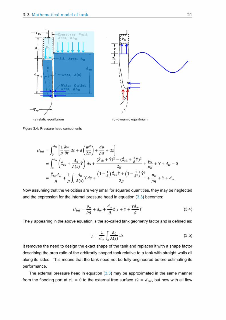
3.2. Mathematical model of tankThe tank is assumed to have two states: an equilibrium state and a dynamic state, seefigure 3.2.

(a) at equilibrium (b) under dynamic conditions

Figure 3.2: Isolated tank [9]

3.2. Mathematical model of tank 19

Assumptions and simplifications:

• incompressible flow

• irrotational flow

• inviscid flow (viscosity is ignored)

• unsteady flow

• the incoming wave has a small slope (small amplitude compared to length)

• the incoming wave is regular

• deep water (> 1000m)

• body has no or small forward speed (a good pipelaying speed is 9 km/day, whilst installationvessels are completely stationary)

• no saturation of the tank occurs

• no ventilation of the flooding port occurs

• sloshing is negligible due to relatively small tank width

The amount of water that flows into the tank must be equal to the water volume increase atthe top of the tank (figure 3.3). The volumetric flow rate for incompressible flow is expressedby rate of flow through the port or rise in water level:

𝑄 = 𝛽𝐴 𝐶 √2𝑔Δ𝐻 = 𝐴 ΥΥ = 𝛽𝐶 √2𝑔Δ𝐻 (3.1)

with 𝐴 the free surface area of the tank,𝛽 the size of the flooding port relative to the free surface area,𝐶 the effective discharge coefficient of the flooding port,Δ𝐻 the differential pressure head over the flooding port [𝑚].

Rewrite to obtain an expression for the water velocity Υ:

|Υ|Υ = 2𝑔𝛽 𝐶 Δ𝐻 (3.2)

Since the water motion Υ is neither real nor strictly positive (when the pressure head is negativeΔ𝐻 < 0, outflow from the tank will occur: Υ < 0), the square of the variable must be describedas the absolute value multiplied with the complex value. In order to determine the watervelocity at the free surface, the pressure head at the flooding port Δ𝐻 needs to be determined.

20 3. Theory

Figure 3.3: Flow rate equality

The differential pressure head over the flooding port is the difference between the externalpressure head and the internal pressure head:

Δ𝐻 = 𝐻 − 𝐻 (3.3)

The above equation is the Bernoulli equation in its simplest form, stating that𝐻 −𝐻 −Δ𝐻 = 0and contains all pressure components. These components depend on the ship/tank motion,the water motion, air pressure in the tank and the incoming wave plus the diffraction andradiation pressures.

Due to the wave(s) in the environment the differential pressure head continuously changesand therewith the volume of water in the tank and subsequently the flow velocity. The consequenceis that both the elevation of the water surface and the flow rate are unknown, requiring anunsteady-flow analysis (instead of the commonly used steady-flow analysis).

To determine the internal pressure head the Bernoulli equation for unsteady flow is derivedin the 𝑧-direction (tank water motion modeled in 1DoF) and integrated over the streamline asdrawn in figure 3.2a: from the flooding port at 𝑠1 = 0 to the internal free surface at equilibrium𝑠2 = 𝑑 .

𝐻 = ∫ 𝐷𝑤𝐷𝑡 𝑑𝑠 = ∫ [𝑑𝑝𝜌𝑔 +

1𝑔𝜕𝑤𝜕𝑡 𝑑𝑠 + 𝑑 (

𝑤2𝑔) + 𝑑𝑧]

Assume that the flow in the tank is essentially one-dimensional along a vertical streamline. Atthe free surface 𝐴(𝑠) = 𝐴 and at the flooding port 𝐴(𝑠) = 𝛽𝐴 , where 𝛽 is the ratio of the sizeof the flooding port to the free-surface area. The instantaneous vertical velocity of the waterat position 𝑠 on the streamline is the sum of the velocity of the tank due to ship motions andthe water velocity relative to the tank:

𝑤 = �� + 𝐴𝐴(𝑠)Υ

3.2. Mathematical model of tank 21

(a) static equilibrium (b) dynamic equilibrium

Figure 3.4: Pressure head components

𝐻 = ∫ [1𝑔𝜕𝑤𝜕𝑡 𝑑𝑠 + 𝑑 (

𝑤2𝑔) +

𝑑𝑝𝜌𝑔 + 𝑑𝑧]

= ∫ (�� + 𝐴𝐴(𝑠)Υ) 𝑑𝑠 +

(�� + Υ) − (�� + Υ)2𝑔 + 𝑝

𝜌𝑔 + Υ + 𝑑 − 0

= �� 𝑑𝑔 + 1𝑔 ∫

𝐴𝐴(𝑠)Υ 𝑑𝑠 +

(1− ) �� Υ + (1− ) Υ2𝑔 + 𝑝

𝜌𝑔 + Υ + 𝑑

Now assuming that the velocities are very small for squared quantities, they may be neglectedand the expression for the internal pressure head in equation (3.3) becomes:

𝐻 = 𝑝𝜌𝑔 + 𝑑 + 𝑑𝑔 �� + Υ + 𝛾𝑑𝑔 Υ (3.4)

The 𝛾 appearing in the above equation is the so-called tank geometry factor and is defined as:

𝛾 = 1𝑑 ∫ 𝐴

𝐴(𝑠) 𝑑𝑠 (3.5)

It removes the need to design the exact shape of the tank and replaces it with a shape factordescribing the area ratio of the arbitrarily shaped tank relative to a tank with straight walls allalong its sides. This means that the tank need not be fully engineered before estimating itsperformance.

The external pressure head in equation (3.3) may be approximated in the same mannerfrom the flooding port at 𝑠1 = 0 to the external free surface 𝑠2 = 𝑑 , but now with all flow

22 3. Theory

directions included. The velocity terms are expressed in velocity potential Φ (derivation isanalogous to 𝐻 ):

𝐻 = −1𝑔𝑑Φ𝑑𝑡 +

∇Φ ⋅ ∇Φ2𝑔 + 𝑝𝜌𝑔 + 𝑑 − 𝑍

Assuming regular waves with a small slope the velocity of the water is small as the wavepasses; the velocities squared are subsequently very small andmay be neglected. This leavesonly the dynamic pressure due to the waves:

𝐻 = −1𝑔𝑑Φ𝑑𝑡 +

𝑝𝜌𝑔 + 𝑑 − 𝑍 = 𝐻 + 𝑝𝜌𝑔 + 𝑑 − 𝑍 (3.6)

At static equilibrium the air and water pressures on the inside and outside are in equilibrium:= + 𝑑 − 𝑑 . Combining this relation and equations (3.4) and (3.6) results in the

following differential pressure head:

Δ𝐻 = 𝐻 − 𝑝 − 𝑝𝜌𝑔 − 𝑍 − 𝑑𝑔 �� − Υ − 𝛾𝑑𝑔 Υ

In the above equation 𝑍 is the collection term for the tank motion in all directions basedon the ship motions. Not all ship motions make a significant contribution to the tank motion.Surge is generally small and can be neglected; assuming that the tanks are located midshipsyaw motions will also be negligible; lastly, the tanks are assumed to have a small width sosloshing and sway motions may also be neglected. The local vertical motion of the tank itselfthen consists of the contributions of the heave, pitch and roll motions of the ship due to theregular wave:

𝑍 = 𝜉 − 𝑥 𝜉 + 𝑦 𝜉

The elaboration on this model is split into the following parts and are treated in the respectivesubsections:

1. dynamic water pressure (𝐻 )

2. dynamic air pressure ( )

Substituting these components into equation (3.3) the differential pressure head for one tankbecomes:

Δ𝐻 = −𝑍 , −𝑑𝑔 �� , −(1+𝑉 )Υ −

𝛾𝑑𝑔 Υ −𝑈Υ +𝜔𝑔 𝜁 (Φ +Φ )𝑒 +𝜔𝑔 ∑ 𝜉 Φ 𝑒

(3.7)Combined with the flow equation (3.2) the tank model becomes:

𝛾𝑑𝑔 Υ + 1

2𝑔𝛽 𝐶 |Υ |Υ +(1+𝑉 )Υ +𝑈Υ = −𝑍 , −𝑑𝑔 �� , +

𝜔𝑔 𝜁 (Φ , +Φ , )+

𝜔𝑔 ∑ 𝜉 Φ , 𝑒

(3.8)

3.2. Mathematical model of tank 23

3.2.1. Dynamic water pressureThe modeling of the dynamic water pressure due to the incoming wave, the diffraction and theradiation is treated in this section. This turned out not to be straightforward as panel pressurescannot be exported from AQWA at the present time. In the VER Model the water pressure atthe flooding port is estimated with a Froude-Krylov pressure plus a motion pressure in the formof a velocity head. To examine the validity of this approach a forced roll motion is applied to thetank model and its results presented at the end of this section. Two other options, modelingthe pressure using the wave elevation or the fluid potentials, are explored first.

Pressure output available fromAQWA The following panel pressures excluding the hydrostaticpressure can be obtained from AQWA-LINE (frequency domain):

• output field point pressure (FPNT),This is the pressure head at a certain predefined point, including only the height of theundisturbed incoming wave and the diffracted wave.

• the total pressure on a panel (PRPR),The total pressure consists of the hydrostatic-varying (i.e. immersion due to motion),radiation (addedmass/damping), Froude-Krylov, and diffraction pressures. This pressureis in (kilo)Pascals, so to acquire the total pressure head in meters the panel pressureneeds to be divided by 𝜌𝑔.

• the modified and unmodified potentials (PRPT),From these unmodified field potentials the total pressure on a panel can be calculatedusing equation (3.9), which is elaborated in the next paragraph.

The total pressure on a panel cannot be used directly in the model, because the radiationpotentials depend on the amplitude of the ship motions. The aim of an anti-roll tank is toreduce the ship motions. If the ship motion is reduced due to anti-roll tank action, the radiationpressure on an element due to ship motions also becomes lower. Consequently, the radiationpressure should be separated from the incoming wave and diffraction pressures. The mostdirect way to obtain the radiation pressure would be to calculate them directly from the potentials.However, from AQWA only the total pressure on an element or the wave elevation (pressuredue to the incoming and diffracted wave) at a certain point on the hull is available. The separateradiation pressures are not given. These can only be determined directly from the potentials.

Modeling of the water pressure in this report The dynamic water pressure head dependson the surrounding field flow velocities. For a stationary ship (no forward speed):

𝐻 = −1𝑔𝜕Φ𝜕𝑡

24 3. Theory

The total potential Φ per unit amplitude wave consists of the incident wave, diffraction andradiation potentials (from AQWA [6]). For one regular wave this is:

Φ = (Φ +Φ + ∑ 𝜉 Φ )𝑒

DELFRAC uses a slightly different definition of the pressure using the potentials than AQWA.According to Pinkster [10]:

𝐻 = 𝜔𝑔 [𝜁 (Φ + Φ ) + ∑ 𝜉 Φ ] 𝑒 (3.9)

These potentials can be obtained from the diffraction program DELFRAC. In cases wherethe potentials were unavailable at the time of the simulations the wave elevation given byAQWA-LINE is used (this is clearly stated with the results for those simulations). The waveelevation (indicated with 𝑧 here) consists of the incoming wave and the diffracted wave,radiation is excluded.

Modeling of the dynamic water pressure in the VERModel In the VERModel the dynamicwater pressure at the flooding port is modeled with a Froude-Krylov pressure plus the rollsubmergence and a velocity head. The validity of using the velocity head is explored here.

ship particulars loading condition tank particulars coefficients𝐿 143 m 𝑚 29210 mt 𝛾 5.8 𝑚 69 t 𝛽 0.28𝐵 36.8 m 𝐾𝐺 11.926 m 𝑙 31.2 m 𝑥 0 m 𝐶 0.37𝐻 15.1 m 𝑇 6.45 m 𝑏 2.3 m 𝑦 17.25 m 𝛼 0.03

𝐺𝑀 9.35 m 𝐴 71.7 m 𝑑 2.55 m 𝐶 0.7𝑇 11.3 s 𝑑 5.45 m 𝑑 5.45 m

Table 3.1: Calculation parameters

At low frequencies (long waves) as 𝜔 → 0, 𝜔 ≈ 0, the water level should be equal to themotion of the tank as the ship moves so slowly that the water level has time enough to adjust.

Υ = 𝑦 𝜑 = 1.765 m

In the upper limit the water level indeed goes to 1.77 meters in the simulation. Note that theoptimum is still at a period of 10 seconds, where the phase lag with respect to the tankmotion is90 degrees. Even though the water level reaches a higher level, the tank will be less effectivedue to the different phase shift (not depicted here).

The initial expectation was that the change in water level goes to zero for high frequencies(very short waves)𝜔 >, 𝜔 ≫, because the water level does not have time to adjust. However,

3.2. Mathematical model of tank 25

(a) amplitude (b) phase shift

Figure 3.5: Water level dependence on excitation frequency, fully vented tanks

this is without taking into account the change in water level due to (unsteady) flow acceleration.These scale with 𝜔 , thus the change in water level does not go to zero for high frequencies.So, the water level should be close to the results of the acceleration terms of the tank and thetank water plus (or rather minus) the hydrodynamic pressure term.

Υ =𝑦 𝜑 −

= 𝑦 𝜑𝛾 (1 − 12

𝑦 𝜑𝑑 ) = 0.373 m

The water level of the tanks in the model goes to 0.32 m in the lower limit, see figure 3.5, whichmatches the above calculated value satisfactorily. This figure also shows that for an excitationperiod of 5 seconds the tank action is (almost) in phase with the ship roll motion, which couldlead to amplification of the ship motion. Interestingly the change in water level goes to zerofor only one point in the graph. The equation for this cancellation point and the associated rollfrequency is:

− 𝑦 𝜑 + 𝜔 𝑑𝑔 𝑦 𝜑 − 𝜔2𝑔𝑦 𝜑 = 0

𝜔 (𝑑𝑔 − 𝑦 𝜑2𝑔 ) = 1

𝜔 = √𝑔

𝑑 − 𝑦 𝜑 /2

Both the equilibriumwater level 𝑑 and the tank arm 𝑦 are constants determined in the designphase, so only the amplitude of forced roll angle is variable. This phenomenon, therefore, doesnot depend on the natural frequency of the ship or the tank transfer period. With increase ofamplitude of forced roll angle, the period at which the water level amplitude goes to zerodecreases.

The period at which the change in water level is zero decreases quadratic with roll angle(see figure 3.6). The limit for zero roll angle seems to be a period of exact 5 seconds. This

26 3. Theory

Figure 3.6: Roll period for cancellation point versus forced roll angle amplitude

is in line with the expectation: as the roll angle amplitude goes to zero, the frequency of rollat which the change in water level is canceled out goes to 1.26 rad/s corresponding to a rollperiod of 5 seconds.

The maximum forced roll angle at which this point exists in this case is around 40 degrees,figure 3.6. The roll frequency quickly rises and goes to infinity as a result of the denominatorgoing to zero: 𝜑 = = 40. For larger forced roll angles the zero point does notexist anymore, because the water acceleration does not become large enough to cancel outthe water level change and the velocity pressure.

So the existence of this cancellation point in figure 3.5 can be explained, however, in realityit will never appear. The cancellation point is only present in this graph as a result of modelingthe dynamic water pressure using the velocity head and not because it is a physical occurringphenomenon.

Even though the influence of the velocity head turns out to be small, it does presenta danger to model the dynamic water pressure using the velocity head, as it can give anon-physical and incorrect result. Because obtaining the velocity head is relatively easy,especially if compared to calculating the pressure using the flow potentials, it is tempting touse it as a simplification of the pressure head problem at the flooding port. However, it can beconcluded that it is important to use the velocity head approximation with caution.

3.2.2. Dynamic air pressure

In this subsection the influence of different layouts of the air venting on the pressure head areexplored. Four different configurations can be distinguished for the top of the tank, table 3.2and figure 3.7.

The dynamic air pressure equation is deduced here for a crossover connected tank. Theproperties of the other air configurations may be inferred from this relation for the air pressure.The homogeneous form for the flow relation of air into and out of a tank is defined according

3.2. Mathematical model of tank 27

fully vented The top of the tank is completely open.unvented The top of the tank is completely closed.separately vented The tank is connected to the outside air through an air vent.crossover connected The tank is connected to the tank on the opposite side by an air duct.

Table 3.2: Passive air configurations

(a) fullyvented

(b) unvented (c) separatelyvented

(d) crossoverconnected

Figure 3.7: Passive air configurations

to Rouse [11]:

�� = 𝜌 𝑄 = 𝜌 ⋅ 𝐶 𝐴 √2Δ𝑝𝜌 = 𝛼𝐶 𝐴 √2𝜌 Δ𝑝 (3.10)

The change in pressure can be described as: Δ𝑝 = (𝑝 −𝑝 )− (𝑝 −𝑝 ) = 𝑝 −𝑝 . Assumeisothermal expansion so that = . The air mass in one tank under equilibrium conditionsis 𝑚 = 𝜌 𝐴 𝑑 . Define the atmospheric pressure 𝑅 , a linearized discharge coefficient 𝑅and a constant describing standard atmospheric conditions 𝑅 in head of water:

𝑅 = 𝑝𝜌𝑔 =

𝑝𝜌𝑔 + 𝑑 − 𝑑

𝑅 = 𝐶 𝑝√|𝑝 − 𝑝 |

𝑅 = √2𝑝𝜌

Substitution of these coefficients into the mass flow equation and its elaboration is given inappendix A. The end result of the derivation is that the air pressure can be expressed using anair pressure constant 𝑉 for the air pressure due to the water level in the tank itself and an airpressure coupling constant 𝑈 to compensate for air crossover effects from the opposite tank:

𝑝 − 𝑝𝜌𝑔 = 𝑉 Υ + 𝑈Υ (3.11)

The definition of the air pressure constants is elaborated upon in the next paragraphs for theair configurations given in table 3.2. The air pressure constants for all air configurations arecollected in table 3.3, which can be found beyond the derivation.

28 3. Theory

Fully vented In the fully vented case both the pressure constant 𝑉 and the pressure couplingconstant 𝑈 are zero, since the air pressure is equal to the atmospheric pressure due to thefully open top and there is no interconnection between the tanks.

Unvented The air pressure change as a result of fluctuating water level needs to be takeninto account, but there is no air crossover between the tanks: 𝑉 is constant and 𝑈 is zero. Asignificant air ”spring constant” is introduced by blocking air flow, which may alter the apparenttank period. Compression of air results in an increase of absolute pressure proportional to thepercentage change in volume. The air pressure constant is the ratio of the static pressurehead to the height of the tank above the equilibrium water level.

𝑅 = 𝑝𝜌 𝑔 + 𝑑 − 𝑑

𝑉 = 𝑅𝑑

If the volume of air above the equilibrium water level is small the water level in the tank willhardly vary, because the air pressure in the tank will increase as much as the water pressure.This is in accord with the findings ofWebster, who found that the Slo-Rol tanks stopped workingwhen the valves in the crossover duct were closed. This means that anti-roll tanks, if sodesigned, can be turned off by closing the air vents.

Separate venting In this case the tank is partially vented with an air vent. The amount of aircan change, but it cannot flow unobstructed in and out of the tank. The equations for the airpressure now include an air escape and entry coefficient to account for outflow and inflow ofair.

𝑅 = 𝑝𝜌 𝑔

𝑅 = 𝐶

√ | |= 𝐶

√|𝑉 Υ |𝑅

𝑉 =𝜔 𝑅 𝑑 + 𝑖𝜔𝛼𝑅 𝑅 𝑅𝜔 𝑑 + 𝛼 𝑅 𝑅

Air crossover connection The tanks are interconnected with an air duct. No externalregulation of the air flow is included in this model.

𝑅 = 𝑝𝜌𝑔 + 𝑑 − 𝑑

𝑅 = 𝐶

√|𝑃 − 𝑃 |𝑅

= 𝐶

√|2𝑃 |𝑅

3.2. Mathematical model of tank 29

𝑈 = 𝛼𝑅 𝑅 𝑅𝑑 ⋅ 2𝛼𝑅 𝑅 − 𝑖𝜔𝑑

𝜔 𝑑 + 4𝛼 𝑅 𝑅

𝑉 = 𝑅𝑑 − 𝑈

Fully vented Unvented Separately vented Crossover connected

discharge coefficient 𝑅 0 0 𝐶 /√ | | 𝐶 /√ | |

air pressure constant 𝑉 0 − 𝑈coupling constant 𝑈 0 0 0

Table 3.3: Overview of the air constants

3.2.3. Unknown parametersThere are three unknown parameters in the tank model, which are not directly chosen bythe tank designer, namely tank geometry factor 𝛾, flooding port discharge coefficient 𝐶 andair discharge coefficient 𝐶 . The tank can be designed such that the tank geometry factorensures that the tank is tuned to the ship natural rolling period in its most common loadingcondition by adjusting the tank transfer period (explained in the next paragraph). The othercoefficients need to be estimated, determined with model experiments or by other means,such as computational fluid calculations.

Tank transfer period The tank transfer period is the parameter on which the tuning of thetank is based as shown in figure 2.3b. It is defined analogous to the transfer period of a U-tubeanti-roll tank. If a ship with a U-tube tank is removed from its upright equilibrium and positionedunder a certain roll angle, the water will flow from the higher tank to the lower tank until thelevel of water in both tanks is equal again. The time it takes to regain an equilibrium waterlevel in the tanks is called the tank transfer period. Now imagine that the free-flooding anti-rolltanks can be thought of as a U-tube tank with an external connection through the surroundingseawater instead of an internal connection tube.

30 3. Theory

The transfer frequency of a U-tube tank is deduced from the tank equation as done byStigter [12]. The coupled equation of motion of tank fluid with ship roll motion in still water asgiven by Stigter:

𝑐 �� + 𝑐 𝜑 + 𝑏 �� + 𝑏 �� + 𝑏 𝜓 = 0

with:𝜑 roll angle of the ship𝜓 relative roll angle of the tank water:

angle between bottom plane of tank and a plane through the center pointsof the free-surfaces of the tanks

𝑐 coupling coefficient of ship inertia into tank fluid motion𝑐 coupling coefficient of ship spring term into tank fluid motion𝑏 added mass coefficient of tank fluid𝑏 damping coefficient of tank fluid𝑏 spring term coefficient of tank fluid

The tank transfer frequency is defined by the spring term coefficient and the inertia coefficient:𝜔 = . Developed and translated to the terminology used in this report, the tank transferfrequency becomes:

𝜔 = √𝑏𝑏 = √0.5𝜌𝑔𝑤 𝑤 𝑙

0.5𝜌𝑤 𝑤 𝑙 ∫ 𝑑𝑠= √

𝑔𝑤 𝑙 ∫ 𝑑𝑠

= √𝑔

𝐴 ∫ ( ) 𝑑𝑠= √

𝑔∫ ( ) 𝑑𝑠

where ∫ ( ) 𝑑𝑠 is the effective length of the U-tube tank connection tube. Changing theeffective length, either by changing the height of the equilibrium water level or cross section ofthe tube, changes the transfer frequency of the tank. Translating this to a free-flooding tank,which again is modeled as a U-tube tank with an external tube, using equation (3.5) results in:

𝑇 = 2𝜋𝜔 = 2𝜋√

∫ ( ) 𝑑𝑠𝑔 = 2𝜋√𝛾𝑑𝑔

According to most authors on anti-roll tanks, the tank transfer period should be equal to orslightly lower than the ship´s natural roll period for optimal performance. Barr and Ankudinov [13],for example, conclude that the tank period should be 6-10% lower than the ship´s naturalperiod for the best performance.

The tank transfer period can be tuned (lengthened) to the ship´s roll period by modifyingthe geometry of the inlet duct, analogous to the tuning of an internally cross-connected U-tubetank. Since the desired tank transfer period is known, an optimum tank geometry factor canbe deduced and used in the mathematical model. The actual shape of the free-flooding tankand inlet duct is not relevant as long as the tank walls are straight around the equilibrium waterlevel. This leaves room for a design that is custom fit, such as the tank shown in figure 3.8.

3.3. Time domain 31

Figure 3.8: Free-flooding anti-roll tank as designed for USS Midway [9]

3.3. Time domainWebster [9] assumes that the system behaves linear, so that the system can be studied infrequency domain. This linear assumption is violated by the non-linear damping in the tanks.In non-linear systems the superposition principle is no longer necessarily valid. However,since the system is only weakly non-linear, the it is likely that a semi-linear approach will alsoapproximate the results of the effect of the anti-roll tank quite well.

This section starts off with the properties of the Webster Model in § 3.3.1 and its solution isderived in § 3.3.2. To determine the properties of the model the situation for a forced roll testwith fully vented tanks is evaluated. For the forced roll test the heave and pitch motions will bevery small, so these can be neglected and the tank motion will consist of pure roll: 𝑍 = 𝑦 𝜙.Also, 𝑉 = 𝑈 = 0 as the tank is fully vented. In a forced roll test there is no pressure due towaves, so there is no wave elevation pressure and the dynamic radiation pressure may beneglected for small roll angles. Equation (3.8) gets stripped to:

𝐶 Υ + 𝐶 |Υ|Υ + Υ = −𝐶 𝑍 (3.12)

with:

𝐶 = 𝛾𝑑𝑔

𝐶 = ( 1𝛽𝐶 √2𝑔

) = 12𝑔𝛽 𝐶

𝐶 = 1 − 𝜔 𝑑𝑔

32 3. Theory

Introduce Υ = 𝑥 and Υ = 𝑦 as functions of time to create the following system of first orderequations:

�� = 𝑦𝐶 �� = −𝑥 − 𝐶 |𝑦|𝑦 − 𝐶 𝑍

or

�� = 1𝐶 ([ 0 𝐶

−1 −𝐶 |𝑦|] 𝑥 − [ 0

𝐶] 𝑍 ) (3.13)

Two numerical methods are applied to a forced roll test and a free decay test in SCILAB, asdescribed in § 3.3.2. For application in the diffraction time domain analysis by AQWA-NAUT aDynamic-Link Library (DLL) has been written in C++. The results of this analysis can be foundin § 4.1.2.

3.3.1. Properties of the non-linear systemThe problem with non-linear equations such as equation (3.12) is that its properties are noteasy to determine. A linear system:

• satisfies the properties of superposition (linearity and homogeneity),

• has one equilibrium point at the origin,

• its stability can be evaluated directly,

• for a sinusoidal input, the output signal only contains one harmonic.

For example, the principle of superposition does not necessarily hold for a forced non-linearsystem and if the input is sinusoidal the output may containmany harmonics and sub-harmonicswith various amplitudes and phase differences. In this section the existence plus uniquenessof equilibrium points and the stability are evaluated for the non-linear system excluding the airpressure and the dynamic pressure head (𝐻 ).

Equilibrium points In order to determine the number (and approximate location) of theequilibrium points of the non-linear equation a phase plot (figure 3.9) of the problem is constructed.The lines in the figure represent the nullclines. These are curves along which the vector fieldis entirely horizontal or entirely vertical; it is the boundary where the derivatives to time 𝑥 and𝑦 change sign. Intersections between the nullclines represent equilibria of the system. Thenullclines can be found by equating the derivative of the system of equations as defined inequation (3.13) to zero:

�� = 𝑦 = 0 (3.14a)

�� = −𝑥 − 𝐶 |𝑦|𝑦 − 𝐶 𝑍𝐶 = 0 (3.14b)

3.3. Time domain 33

So, the 𝑥-nullcline is given by 𝑦 = 0 and the 𝑦-nullcline is the curve 𝑥 = −𝐶 |𝑦|𝑦 − 𝐶 𝑍 . Thearrangement of the nullcline curves in figure 3.9 discloses that the solutions circle around oneequilibrium point. This cycle represents a linear oscillation.

(a) phase plot (b) trajectory

Figure 3.9: Equilibrium point analysis non-linear equation

In this particular case the only equilibrium point can simply be determined by inserting theresult from (3.14a) into (3.14b):

�� = 0 = −𝑥 − 𝐶 |0|0 − 𝐶 𝑍𝐶 ⇒ 𝑥 = −𝐶 𝑍

The equilibrium point is thus 𝑎 = (−𝐶 𝑍 , 0).

Stability As there is only one equilibrium point, the stability of the system is consideredaround this point. It is not possible to directly assess the behavior of the non-linear equation,therefore it is linearized in the neighborhood of equilibrium point 𝑎 = (−𝐶 𝑍 , 0). The linearizationof �� is the linear function given by:

𝐿(𝑥) = 𝑓(𝑎) + 𝜕𝑓(𝑎)𝜕(𝑥, 𝑦) (𝑥 − 𝑎)

The derivative of the non-linear equation is:

𝜕𝑓𝜕(𝑥, 𝑦) =

1𝐶 [ 0 𝐶

−1 −2𝐶 √𝑦]

34 3. Theory

Around equilibrium point 𝑎 = (−𝐶 𝑍 , 0):

𝑓(𝑎) = 1𝐶 [ 0

𝐶 𝑍 − 𝐶 |0|0 − 𝐶 𝑍] = [0

0]

𝜕𝑓(𝑎)𝜕(𝑥, 𝑦) =

1𝐶 [ 0 𝐶

−1 0]

The result of linearizing the equations (3.14):

�� = 1𝐶 [ 0 𝐶

−1 0] [𝑥 + 𝐶 𝑍

𝑦 − 0] = 1

𝐶 [ 𝐶 𝑦−𝑥 − 𝐶 𝑍

]

= 1𝐶 ([ 0 𝐶

−1 0] 𝑥 + [0

1] 𝐶 𝑍 )

The solution of the linearized system is:

𝑑𝑦𝑑𝑥 =

1𝐶−𝑥 − 𝐶 𝑍

𝑦𝐶 ∫𝑦 𝑑𝑦 = ∫(−𝑥 − 𝐶 𝑍 )𝑑𝑥12𝐶 𝑦 = −12𝑥 − 𝐶 𝑍 𝑥 + 𝐶 = −12𝑥 − 𝐶 𝑍 𝑥 − 12(𝐶 𝑍 )

𝑦 = √−𝑥 − 2𝐶 𝑍 𝑥 − (𝐶 𝑍 )𝐶 = √(𝑥 + 𝐶 𝑍 )(−𝑥 − 𝐶 𝑍 )𝐶

The eigenvalues belonging to this system of equations are:

𝐴 − 𝜆𝐼 = 0

[ −𝜆 1−1/𝐶 −𝜆

] = 𝜆 + 1𝐶 = 0

𝜆 = − 1𝐶

𝜆 , = ±√1𝐶 𝑖 = ±𝜔𝑖

The solution of the eigenvalues is purely imaginary, signifying that the equilibrium point is acenter. The orbits rotate clockwise around the origin, since �� > 0 when 𝑥 = 0 and 𝑦 > 0. Thesystem is stable and periodic with a period 𝑇 = . The amplitude of the system oscillation isdetermined by the initial conditions.

Consequently, it is assumed here that temporarily separating the tank fluid dynamics fromthe ship dynamics, as stipulated for the frequency domain § 3.1, is still justified for the timedomain.

3.3. Time domain 35

3.3.2. Solving the systemThe problem can be solved in the time domain by applying a numerical integrator to solve thesystem of equations. The most commonly used fixed step methods are evaluated on basis ofstep size, maximum error and calculation time by introducing a linear test case equation. Thereason for using a test equation and not the non-linear equation describing the real problem isthat the solution to the non-linear equation is unknown, thus giving no means of determiningthe error between the approximated value with the numerical method and the real value.

To be able to solve the system of equations with implicit methods such as Backward Euler,the non-linear term needs to be linearized. This is done by taking one of the water velocitiesin the non-linear term at the old time step 𝑛 and the other at the new time step 𝑛+1: |𝑦 |𝑦 .In the explicit methods the current estimate for the water velocity at each intermediate timestep is used.

As determined in § 3.3.1 only the properties of the linearized problem can be judged.Consequentially, for comparison of the numerical integrators and testing their suitability alinear test case, which is similar to the non-linear problem, needs to be used. The test equationchosen is 𝐶 �� + 𝑦 = 0 with the solution 𝑦 = cos(𝜔𝑡). Since the solution to this linear problemis known, the methods can be evaluated on accuracy by means of the global error. Thiserror consists of all the local errors made over time and thus grows as time progresses, seefigure 3.10.

Figure 3.10: Global error for the Modified Euler method

There are many different numerical methods available for solving all kinds of problems.The methods explored in this report are all single-step methods, subdivided in two categories:fixed step methods and variable step methods. Fixed step methods use a constant step sizeall through the calculation, while variable step methods optimize the step size on the basisof the local truncation error. Fixed step methods are still applied the most frequently, but areslowly replaced by variable step methods.

36 3. Theory

The most commonly used numerical methods are compared on the produced global errorafter four periods and their computing times. The numerical method combining a small globalerror with a short calculation time is considered the optimal choice for use in solving the systemof equations.

Fixed step methodsFive fixed step methods have been evaluated on efficiency and accuracy, namely ForwardEuler, Backward Euler, Modified Euler, the Trapezoidal method and Runge-Kutta. The stepsize is inversely related to the computation time, i.e. a long computation time is the result oftaking small steps.

(a) largest possible step size (b) error same order of magnitude

Figure 3.11: Computation time and error of fixed step methods (visibly smooth and matching the exact solution)

The Forward Euler and Backward Euler methods are notable in figure 3.11a due to thelong computing time and relative inaccuracy. These methods are consequently dropped fromconsideration. Next, the remaining methods are compared on computation time when theglobal errors have the same order of magnitude (see figure 3.11b). The method combining ashort computing time with high accuracy in the category fixed step methods is the Runge-Kuttamethod.

Variable step methodsThese methods are less commonly found, probably because the routine is more complicated.However, they have two significant advantages over fixed step methods:

1. The step size is determined automatically, removing the chance that the result becomesunbounded or inaccurate (especially for the small frequencies).

2. The calculation time is shorter due to the optimization of the step size.

3.3. Time domain 37

To start with three variable step methods have been evaluated on efficiency and accuracyin figure 3.13a, namely Heun-Euler, Bogacki-Shampine and Runge-Kutta-Fehlberg. It turnsout that the time step needs to be extremely small for the Runge-Kutta-Fehlberg method tomore or less follow the exact solution, which means that it is unstable for the test case. Thisinstability can be seen in figure 3.12. There are more known instances where the RKF45method is unstable; a common example of failure of the Runge-Kutta-Fehlberg method isgiven by Skufca [14]. Due to general problems with the RKF-algorithm an alternative, morestable, 5th order Runge-Kutta method was developed by Cash and Karp [15], called theCash-Karp method. This method does converge to the exact solution. It follows that theRunge-Kutta-Fehlberg method is dropped from consideration due to the long computing timenecessary to gain an acceptable solution (figures 3.13a and 3.13b).

Figure 3.12: Instability of the Runge-Kutta-Fehlberg method

(a) largest possible step size (b) error same order of magnitude

Figure 3.13: Computation time and error of variable step methods (visibly smooth and matching the exact solution)

38 3. Theory

For the test case an optimum value for the desired maximum error Δ = 1𝑒 was found.Again the remaining methods are compared when the global errors have the same order ofmagnitude, figure 3.13b. The method combining a short computing time with high accuracy inthe category variable step methods is the above introduced Cash-Karp method.

Choice of numerical method

Variable stepping is advantageous over fixed stepping in two ways:

1. no mismatch between wave frequency and time step can occur, because the time stepis adjusted automatically;

2. the running time is shorter due to the optimization of the time step.

However, AQWA can only handle fixed steps and one of the objectives is to calculate the shipmotions using the time domain solver AQWA-NAUT. For the tank moment calculation routineimplemented in AQWA-NAUT the fixed step solver Runge-Kutta is used, since this methodcombines speed with accuracy in the category fixed step solvers. Variable step methods areincluded in this report because the optimum step size depends on the wave frequency and forthe routine in SCILAB there is no restriction to fixed methods. A mismatch in wave frequencyand time step leads to erroneous results. To prevent this from happening a variable steppingmethod is used for the SCILAB routine.

3.3.3. Coupling with ship motionsThe ship is modeled with the equilibrium tank water volume included as if it were frozen water.The excitation forces of the ship come from regular waves.

Ship motions The ship motions can be described as follows:

(𝑀 +𝑀 )�� + 𝐶�� + 𝐾𝑥 = 𝐹 (3.15)

The ship mass matrix around its center of gravity is defined as:

𝑀 =

⎡⎢⎢⎢⎢⎢⎢⎢⎣

𝑚 0 0 0 0 00 𝑚 0 0 0 00 0 𝑚 0 0 00 0 0 𝐼 0 −𝐼0 0 0 0 𝐼 00 0 0 −𝐼 0 𝐼

⎤⎥⎥⎥⎥⎥⎥⎥⎦

Since the ship motions are calculated using linear ship motion theory, they are also sinusoidal,meaning that the system of equations can be simplified to:

[−𝜔 (𝑀 +𝑀 ) − 𝑖𝜔𝐶 + 𝐾]𝑥 = 𝐹

3.3. Time domain 39

Tank forces on ship The vertical force exerted upon the ship by a single tank as a result ofthe changes in water level is:

𝐹 = −𝜌𝑔𝐴 [1 − 𝜔 𝑑𝑔 ]Υ

The summation of this vertical force over all tanks is the heaving force exerted by the tankson the ship. The tanks are placed in the midship section, where the sides of the ship and thetank are assumed to be vertical in the area of interest around the waterline.

Similarly, a pitching moment is produced by the sum over the tanks of 𝑥 𝐹. A small lengthof the tank plus placement midships in length ensures that the arm of the pitch moment bythe tank water is very small and the tank pitch moment consequently does not influence thepitch of the ship. Webster considers the terms due to heave and pitch motions of the ship tobe constant and transfers them to the excitation side of the tank equations. This reduces thenumber of degrees of freedom from six to three. However, it is not much more complex to takethese terms into account, so the system of equations is kept in 6DoF.

The relative small width of the tanks also means that phenomena such as sloshing may beneglected. Therefore it is assumed that there is no net lateral force due to a change in waterlevel. The surge, sway and yaw ship motions will not be influenced by these respective forcesdue to tank water level changes, but only through coupling with the tank roll moment.

And last, the tanks generate a net rollingmoment from the summation of the roll moment 𝑦 𝐹over all tanks. The roll moment amplitude for a tank pair (one on port side, another onstarboard) can be written as:

𝐹 = 𝑦 𝐹 = −𝜌𝑔𝐴 [1 − 𝜔 𝑑𝑔 ] 𝑦 (Υ − Υ )

The total force exerted on the ship by a tank pair is:

𝐹 = −𝜌𝑔𝐴 [1 − 𝜔 𝑑𝑔 ]

⎡⎢⎢⎢⎢⎢⎢⎢⎣

00

𝑌 + 𝑌𝑦 (𝑌 − 𝑌 )−𝑥 (𝑌 + 𝑌 )

0

⎤⎥⎥⎥⎥⎥⎥⎥⎦

(3.16)

Assembly of system components The tank motions and force terms are added to the shipmotion equations, retaining the algebraic form 𝐴𝑥 = 𝐵:

𝐴𝑥 = 𝐹 + 𝐹 (3.17)

where 𝐴 consists of the ship mass plus inertia 𝑀, added mass 𝑀 , damping 𝐶 and restoration𝐾 data of the ship, including the equilibrium tank condition. This equation is used in conjunctionwith the equation for the tank (3.8).

40 3. Theory

3.4. Frequency domainWebster approaches the problem in a slightly different way following Blagoveshchensky [16]in order to avoid the quadratic water velocity term. The result is the same system of equationssolved from another angle. Starting from equation (3.1):

Υ = 𝛽𝐶 √2𝑔 Δ𝐻1

√2𝑔 𝛽𝐶Υ = √Δ𝐻 (⋅√Δ𝐻)

√Δ𝐻√2𝑔 𝛽𝐶

Υ = Δ𝐻

√|Δ𝐻| 𝑒 /

√2𝑔 𝛽𝐶Υ = Δ𝐻

with 𝜙 = arctan( ℑ( )ℜ( )). The influence of the phase shift in the pressure head on the water

level increases as 𝛾 gets closer to 1 and 𝛽 decreases. So, only for very small flooding portsizes combined with a completely straight tank the phase shift plays a role. This means thatthe effect of the phase shift in the pressure head can be considered negligible, resulting in:

√|Δ𝐻|√2𝑔 𝛽𝐶

Υ = Δ𝐻 (3.18)

Due to the dependence of both sides of the equation on Δ𝐻, the problem needs to be solvediteratively, reevaluating the differential pressure head until an equilibrium is reached. Thereason that this exact same approach is not used in the time domain calculations is that thesimulations turned out to be unstable (figure 3.14):

1. The solution to the equations (3.7) and (3.18) is unstable if the tank water accelerationterms due to the unsteady flow are included.

Figure 3.14: Change in water level in the time domain including acceleration terms

3.4. Frequency domain 41

If the tank water acceleration terms are omitted from equation (3.7) the solution is stable,but not problem-free as the result is still non-realistic (figure 3.15):

2. The acceleration terms are unrealistically large (especially for high frequencies) andsharply peaked. The velocity curve has a steep slope in the area where the pressurehead changes sign, which results in very large accelerations at these turning points.

3. For small frequencies the calculation of the acceleration terms show acceleration oscillationswhere the water velocity is close to zero.

(a) ≫ (b) ≪

Figure 3.15: Change in water level in the time domain excluding acceleration terms

These problems were resolved by simply redefining equation (3.1) such that the square rootof the pressure head is eliminated, as done in equation (3.2).

Additional tank damping From model experiments on Slo-Rol tanks (§ 2.1) Webster foundindication of the existence of a small linear component of tank damping alongside the non-linearcomponent for the Slo-Rol tanks. Because the practice for U-tube tanks is to include anexperimentally determined linear tank damping in the performance predictions, it is advisableto perform experiments to determine whether a linear tank damping coefficient is applicablefor externally connected tanks. The linear tank damping is integrated in the model as follows:

Δ𝐻 = ( √|Δ𝐻|√2𝑔 𝛽𝐶

+ 2𝐶 √𝛾𝑑𝑔 ) Υ

SinceWebster did not find a linear tank damping coefficient in his tests with the tuned free-floodinganti-roll tanks and no further information is known, it is omitted in the model in this report.

42 3. Theory

3.4.1. Coupling with ship motions

The assumption that a sinusoidal input results in a sinusoidal output for this non-linear equationis considered proven from the results in the time domain section and will be used here tocombine the tanks and the tank action with the ship motions in one complete system ofequations using the coupling relations established in § 3.3.3. The change in water level canthen be described with:

Υ = Υ 𝑒 ,

where Υ represents the complex amplitude of the tank water motion with respect to theincoming wave. Extending the tank motion in the same way, the tank equation (3.8) changesto:

−𝜔 𝛾𝑑𝑔 Υ , 𝑒 − 𝑖𝜔 √Δ𝐻

√2𝑔 𝛽𝐶Υ , 𝑒 + (1 + 𝑉 )Υ , 𝑒 + 𝑈Υ 𝑒

= −𝑍 , 𝑒 + 𝜔 𝑑𝑔 𝑍 , 𝑒 + 𝑧 𝑒 + 𝜔𝑔 ∑ 𝜉 Φ 𝑒

The time term 𝑒 cancels out, transforming the equation from time domain to frequencydomain. With the terms rearranged conveniently for the next step:

(1 − 𝜔 𝑑𝑔 )𝑍 , −

𝜔𝑔 ∑ 𝜉 Φ + (1 − 𝜔 𝛾𝑑

𝑔 + 𝑉 − 𝑖𝜔 √|Δ𝐻|𝛽𝐶 √2𝑔

)Υ , + 𝑈Υ ,

= 𝑧 ,

The associated equation for the pressure head from equation (3.7) is:

Δ𝐻 = −(1 − 𝜔 𝑑𝑔 )𝑍 , − (1 − 𝜔

𝛾𝑑𝑔 + 𝑉 )Υ , − 𝑈Υ , + 𝑧 + 𝜔𝑔 ∑ 𝜉 Φ (3.19)

3.4. Frequency domain 43

The tank is coupled to the ship motion equations, retaining the algebraic form 𝐴𝑥 = 𝐵 fromequation (3.17):

𝐴 =

⎡⎢⎢⎢⎢⎢⎢⎢⎢⎢⎢⎣

𝐴 𝐴 𝐴 𝐴 𝐴 𝐴 0 0𝐴 𝐴 𝐴 𝐴 𝐴 𝐴 0 0𝐴 𝐴 𝐴 𝐴 𝐴 𝐴 𝐶 𝐶𝐴 𝐴 𝐴 𝐴 𝐴 𝐴 𝐶 𝑦 −𝐶 𝑦𝐴 𝐴 𝐴 𝐴 𝐴 𝐴 −𝐶 𝑥 −𝐶 𝑥𝐴 𝐴 𝐴 𝐴 𝐴 𝐴 0 0

− 𝜙 − 𝜙 (𝐶 − 𝜙 ) (𝐶𝑦 − 𝜙 ) −(𝐶𝑥 + 𝜙 ) − 𝜙 𝐺 𝑈− 𝜙 + 𝜙 (𝐶 − 𝜙 ) −(𝐶𝑦 − 𝜙 ) −(𝐶𝑥 + 𝜙 ) + 𝜙 𝑈 𝐺

⎤⎥⎥⎥⎥⎥⎥⎥⎥⎥⎥⎦

𝑥 =

⎡⎢⎢⎢⎢⎢⎢⎢⎢⎢⎢⎣

𝜉𝜉𝜉𝜉𝜉𝜉ΥΥ

⎤⎥⎥⎥⎥⎥⎥⎥⎥⎥⎥⎦

𝐵 =

⎡⎢⎢⎢⎢⎢⎢⎢⎢⎢⎢⎣

𝐹𝐹𝐹𝐹𝐹𝐹𝑧 ,𝑧 ,

⎤⎥⎥⎥⎥⎥⎥⎥⎥⎥⎥⎦

(3.20)

with 𝐶 = [1− ], 𝐶 = 𝜌𝑔𝐴 [1− ] and 𝐺 is the collection term for the tank waterdynamics:

𝐺 = 1 − 𝜔 𝛾𝑑𝑔 + 𝑉 − 𝑖𝜔 √|Δ𝐻|

𝛽𝐶 √2𝑔(3.21)

The complex motion amplitudes 𝜉 and the complex excitation force and moment amplitudes𝐹 have been divided by the wave amplitude 𝜁 to achieve the normalized form per amplitudewave. The system of equations can be extended to include multiple tank pairs.

The system of equations cannot be solved directly, since the coefficients involving tankdynamics are interdependent due to their non-linear nature, but needs to be solved iteratively.With a trial solution for the response vector 𝑥 the air pressure head in equation (3.11) isestimated with which the complex air constants 𝑉 and 𝑈 are determined from table 3.3. Thedifferential pressure head Δ𝐻 (equation (3.19)) is updated with this result and thence thecomplex coefficients of tank transfer function, equation (3.21). The system of equations (3.20)is solved and compared with the result from the previous iteration. The process is repeateduntil the desired tolerance requirement has been met.

4Results

In this chapter the results of the various simulations are presented and discussed. The chapterstarts of with an overview of the particulars of the case presented and follows through with theresults from different simulations.

The mathematical model in chapter 3 is based on a regular wave input. However, theexpected ship motions are best estimated with a viscous damping based on an irregular wavespectrum. The viscous damping in the frequency domain is therefore iteratively adjustedto give a more realistic result for the RAOs and the expected tank performance. The timesimulations are only based on regular wave input, because it is laborious to create a frequencyresponse spectrum from the time simulations and produces no additional information withrespect to the frequency domain analysis of the expected tank performance.

A frequency domain simulation gives the most useful information for engineering purposesas it directly shows the expected motion responses of the ship over a whole range of wavefrequencies. Its results can be found in § 4.2. To verify the frequency domain model, direct andindirect time domain simulations with AQWA-NAUT are explored in § 4.1. To check these timedomain results and specify points of interest a time domain simulation in SCILAB is utilized.The input for the time domain simulations are the RAOs and the wave loads on the vessel.

Lastly the results are compared in the discussion with one another based on simulationtype, air vent configuration and other noteworthy aspects. Also, a parameter study is performedinto different parameters in the tank model. This gives an indication of how tank performancecan be optimized, because the tank moment is directly dependent on the tank water level, seeequation (3.16).

The method used to define the effectiveness of the anti-roll tanks in the previous studiescited in this report is to find the roll response at the resonance frequency in beam seas forthe stabilized and the unstabilized ship and determine the percentage reduction in roll motion.This gives largest roll reduction feasible by the anti-roll tanks, but may not lead to the mosteffective system in all conditions, see Chaplin [17]. However, for ease of comparison in thisreport the tank performance is defined by the roll response at resonance frequency.

45

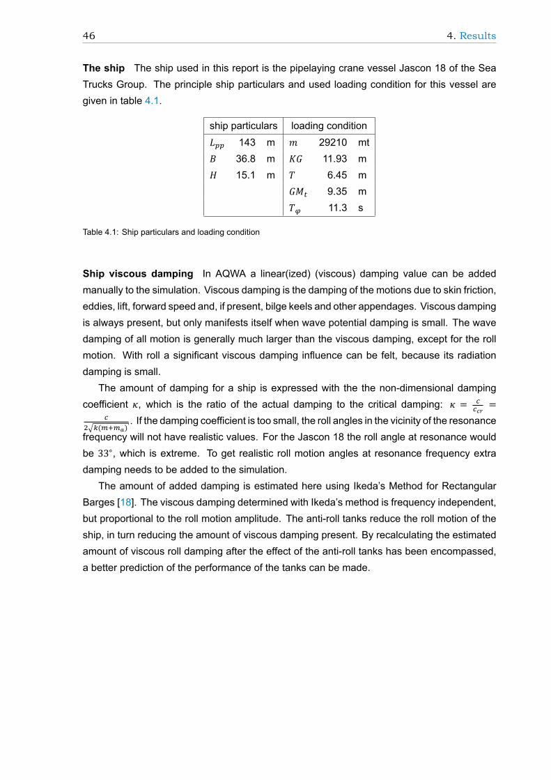
46 4. Results

The ship The ship used in this report is the pipelaying crane vessel Jascon 18 of the SeaTrucks Group. The principle ship particulars and used loading condition for this vessel aregiven in table 4.1.

ship particulars loading condition𝐿 143 m 𝑚 29210 mt𝐵 36.8 m 𝐾𝐺 11.93 m𝐻 15.1 m 𝑇 6.45 m

𝐺𝑀 9.35 m𝑇 11.3 s

Table 4.1: Ship particulars and loading condition

Ship viscous damping In AQWA a linear(ized) (viscous) damping value can be addedmanually to the simulation. Viscous damping is the damping of the motions due to skin friction,eddies, lift, forward speed and, if present, bilge keels and other appendages. Viscous dampingis always present, but only manifests itself when wave potential damping is small. The wavedamping of all motion is generally much larger than the viscous damping, except for the rollmotion. With roll a significant viscous damping influence can be felt, because its radiationdamping is small.

The amount of damping for a ship is expressed with the the non-dimensional dampingcoefficient 𝜅, which is the ratio of the actual damping to the critical damping: 𝜅 = =

√ ( ). If the damping coefficient is too small, the roll angles in the vicinity of the resonance

frequency will not have realistic values. For the Jascon 18 the roll angle at resonance wouldbe 33∘, which is extreme. To get realistic roll motion angles at resonance frequency extradamping needs to be added to the simulation.

The amount of added damping is estimated here using Ikeda’s Method for RectangularBarges [18]. The viscous damping determined with Ikeda’s method is frequency independent,but proportional to the roll motion amplitude. The anti-roll tanks reduce the roll motion of theship, in turn reducing the amount of viscous damping present. By recalculating the estimatedamount of viscous roll damping after the effect of the anti-roll tanks has been encompassed,a better prediction of the performance of the tanks can be made.

47

(a) RAOs excluding viscous damping

(b) RAOs including viscous damping

Figure 4.1: RAOs of roll with and without viscous damping

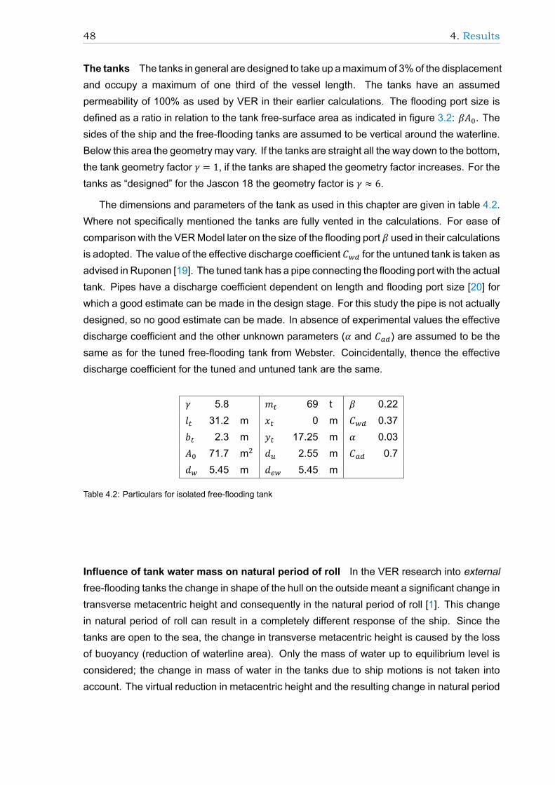
48 4. Results

The tanks The tanks in general are designed to take up amaximumof 3%of the displacementand occupy a maximum of one third of the vessel length. The tanks have an assumedpermeability of 100% as used by VER in their earlier calculations. The flooding port size isdefined as a ratio in relation to the tank free-surface area as indicated in figure 3.2: 𝛽𝐴 . Thesides of the ship and the free-flooding tanks are assumed to be vertical around the waterline.Below this area the geometry may vary. If the tanks are straight all the way down to the bottom,the tank geometry factor 𝛾 = 1, if the tanks are shaped the geometry factor increases. For thetanks as “designed” for the Jascon 18 the geometry factor is 𝛾 ≈ 6.

The dimensions and parameters of the tank as used in this chapter are given in table 4.2.Where not specifically mentioned the tanks are fully vented in the calculations. For ease ofcomparison with the VERModel later on the size of the flooding port 𝛽 used in their calculationsis adopted. The value of the effective discharge coefficient 𝐶 for the untuned tank is taken asadvised in Ruponen [19]. The tuned tank has a pipe connecting the flooding port with the actualtank. Pipes have a discharge coefficient dependent on length and flooding port size [20] forwhich a good estimate can be made in the design stage. For this study the pipe is not actuallydesigned, so no good estimate can be made. In absence of experimental values the effectivedischarge coefficient and the other unknown parameters (𝛼 and 𝐶 ) are assumed to be thesame as for the tuned free-flooding tank from Webster. Coincidentally, thence the effectivedischarge coefficient for the tuned and untuned tank are the same.

𝛾 5.8 𝑚 69 t 𝛽 0.22𝑙 31.2 m 𝑥 0 m 𝐶 0.37𝑏 2.3 m 𝑦 17.25 m 𝛼 0.03𝐴 71.7 m 𝑑 2.55 m 𝐶 0.7𝑑 5.45 m 𝑑 5.45 m

Table 4.2: Particulars for isolated free-flooding tank

Influence of tank water mass on natural period of roll In the VER research into externalfree-flooding tanks the change in shape of the hull on the outside meant a significant change intransverse metacentric height and consequently in the natural period of roll [1]. This changein natural period of roll can result in a completely different response of the ship. Since thetanks are open to the sea, the change in transverse metacentric height is caused by the lossof buoyancy (reduction of waterline area). Only the mass of water up to equilibrium level isconsidered; the change in mass of water in the tanks due to ship motions is not taken intoaccount. The virtual reduction in metacentric height and the resulting change in natural period

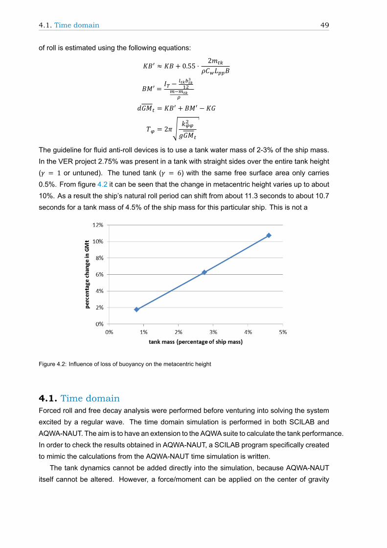
4.1. Time domain 49

of roll is estimated using the following equations:

𝐾𝐵 ≈ 𝐾𝐵 + 0.55 ⋅ 2𝑚𝜌𝐶 𝐿 𝐵

𝐵𝑀 = 𝐼 −

𝑑𝐺𝑀 = 𝐾𝐵 + 𝐵𝑀 − 𝐾𝐺

𝑇 = 2𝜋√ 𝑘𝑔𝐺𝑀

The guideline for fluid anti-roll devices is to use a tank water mass of 2-3% of the ship mass.In the VER project 2.75% was present in a tank with straight sides over the entire tank height(𝛾 = 1 or untuned). The tuned tank (𝛾 = 6) with the same free surface area only carries0.5%. From figure 4.2 it can be seen that the change in metacentric height varies up to about10%. As a result the ship’s natural roll period can shift from about 11.3 seconds to about 10.7seconds for a tank mass of 4.5% of the ship mass for this particular ship. This is not a

Figure 4.2: Influence of loss of buoyancy on the metacentric height

4.1. Time domainForced roll and free decay analysis were performed before venturing into solving the systemexcited by a regular wave. The time domain simulation is performed in both SCILAB andAQWA-NAUT. The aim is to have an extension to the AQWAsuite to calculate the tank performance.In order to check the results obtained in AQWA-NAUT, a SCILAB program specifically createdto mimic the calculations from the AQWA-NAUT time simulation is written.

The tank dynamics cannot be added directly into the simulation, because AQWA-NAUTitself cannot be altered. However, a force/moment can be applied on the center of gravity

50 4. Results

through an external Dynamic Link Library (DLL). The function of a DLL is to import/exportfunctions and data to/from a programwithout changing the core program. Themoment generatedby the tank as a result of the change in water level is fed to AQWA-NAUT through this DLL.The DLL is created here using C++.

For the time domain simulation the Webster Model is adhered to as described in § 3.3.Because the response at the resonance frequency is by far the largest, it is the primaryfocus of interest and therefore only the response at resonance is shown in this report. Theresponse is including the dynamic radiation pressure calculated with the potentials as shownin equation (3.9).

The input regarding tank parameters and settings for the calculations is collected in anexcel sheet. From this excel sheet the variables are imported in SCILAB. The tank is “tuned”to the ship natural period of roll by adapting the tank geometry factor through the equation:

𝛾 = 𝑔𝑑 ⋅ (

𝑇2𝜋)

Even though the area of the tank varies with the height; it is not dependent on the height:

∫ 𝐴(𝑠)𝑑𝑠 = 𝐴(𝑠) | 𝑑 = 𝑉

∫ 1𝐴(𝑠) 𝑑𝑠 =

𝑑𝐴(𝑠)|

This means that the required free surface area of tank for a certain mass of seawater (% ofdisplacement) can be calculated based on the tank geometry factor and the equilibrium waterheight:

𝛾𝑑 = ∫ 𝐴𝐴(𝑠)𝑑𝑠 =

𝐴 𝑑𝐴(𝑠)|

𝐴 = 𝛾𝑑 𝐴(𝑠)|𝑑 = 𝛾𝑉

𝑑 = 𝛾𝑚𝜌𝑑

Input definition One of the initial encountered problems was that the shape of the curves isnot physically correct as can be seen in figures 4.3 and 4.4: for a sinusoidal input the outputshould also be sinusoidal even if the equations are non-linear. This turned out to be a limitationin both SCILAB and AQWA-NAUT: the input needs to be declared as a complex number (asa sinusoidal with a certain phase) in order for the numerical computing environment to takeinto account any phase shifts between the input and the output. If the phase is not explicitlydeclared the program will treat all the variables as reals and ignore phase shifts, giving anon-physically correct output. Consequently, the input needs to be described in the form 𝐴𝑒and cannot be declared as 𝐴 cos(𝜔𝑡) or 𝐴 sin(𝜔𝑡).

In AQWA-NAUT this is problematic, because even though complex numbers are used inthe main routine, only real values are imported into the DLL. So the phase of inputs is only

4.1. Time domain 51

introduced into the non-linear tank equation for the terms that are independent of the tankposition and velocity.

Figure 4.3: Non-physical result SCILAB

-1.5

-1

-0.5

0

0.5

1

1.5

0 5 10 15 20 25 30 35 40 45 50

wat

er

leve

l [m

]

t [s]

Water level

non-linear_tank_eq

linear_tank_eq

Figure 4.4: Non-physical result AQWA-NAUT

4.1.1. indirect AQWA-NAUT simulation

Next the option to add the effect of the tank moment indirectly to the time simulation wasexplored. Instead of calculating the tank moment directly during the time simulation, thetank damping is estimated using a free decay test on the ship motion data and an equivalentdamping is determined. This equivalent damping is used to estimate the tank moment actingon the ship. The equivalent tank damping is only related to the roll angle of the ship, itsmass and transverse metacentre; greatly reducing the number of variables. Also, the phasedependency vanishes, removing the problem in the previous section withmissing phase values.

In this section the free decay analysis is explained and performed on the ship excludingviscous damping to try to estimate the tank damping as accurately as possible. The tankmoment based on the equivalent damping is fed into AQWA-NAUT and the result from thetime simulation is shown.

52 4. Results

Free decay analysisThe equivalent damping coefficient of the tank can be determined with a free decay analysis. Afree decay test takes place in still water. The ship is given a displacement in a certain direction(in this case an initial roll angle since the aim of the anti-roll tanks is to reduce the roll motion),is released and starts rolling. These motions decay and die out, since there is no externalexciting force acting on the ship. The time it takes for the motion to die out and the decreasein maximum motion value are an indication for the damping the tank generates. Since theonly motion of interest is the roll motion, the equations of motion (3.15) can be reduced to oneequation describing a pure roll motion:

(𝐼 + 𝑚 )�� + 𝐶 �� + 𝐾 𝜑 = 𝐹 +𝑀

A free decay test takes place in still water, so the exciting force 𝐹 is zero. The input for thefree decay is a starting position. The test is performed for several initial roll angles; in this case5, 10, 15 and 20 degrees were applied. Viscous damping of the roll motion is not taken intoaccount, in order to try and capture purely the tank damping. At each time step the position ofthe tank is estimated using the acceleration and velocity from the previous time step:

�� = 𝑀 − 𝐾 𝜑 − 𝐶 ��𝐼 + 𝑚

�� = �� + ℎ �� = �� + ℎ ⋅ 𝑀 − 𝐾 𝜑 − 𝐶 ��𝐼 + 𝑚

𝜑 = 𝜑 + ℎ ⋅ �� + ��2

with:𝑀 = −𝜌 𝑔𝐴 (1 − 𝜔 𝑑

𝑔 )𝑦 (Υ − Υ )

In appendix C damping of the roll motion is described using a linear and a quadraticdamping coefficient (courtesy of MARIN). However, the curve in figure 4.5b is not straight asin the appendix, but curved strongly. This shows that the tank damping is indeed non-linear.This non-linear curve cannot be approximated by the general approach using a linear plus aquadratic coefficient, instead we opted for a regression analysis in order to describe the curvemore accurately. It was found that the non-linear data set can best be described with a thirddegree logarithmic equation:

𝑏 + 𝑏 ln(𝜑) + 𝑏 ln (𝜑) + 𝑏 ln (𝜑)

With the damping curve equation and the known roll motion amplitude of the ship includingviscous damping (4.8 degrees in this case) the equivalent damping coefficient of the free-floodingtank can be determined. Note that the curve equation is expressed in radians for the reasonthat the roll angle in the AQWA-NAUT calculation is in radians. The equivalent dampingcoefficient can be used as an alternative input into AQWA-NAUT instead of the direct calculationof the tank moment in the DLL.

4.1. Time domain 53

(a) tank & water motion (b) equivalent damping coefficient

Figure 4.5: Free decay test

Solution convergence Figure 4.6a (created using a fixed step Runge-Kutta solver) showsthat a minimum number of steps needs to be taken per period in order to achieve a convergedsolution for the free decay test. In order to average this number of steps per period the overalltolerance level of the simulation must be set appropriately. There is a trade-off betweenaccuracy and computing time (figure 4.6b). An overall tolerance level of 1𝑒 is chosen asthe optimum between computing time and accurate decrease in peak values.

Results of the indirect time simulationThe tankmoment for the indirect time simulation is based on the equivalent damping coefficientand the roll velocity (see appendix C):

𝑀 = −𝑐𝜋𝜔𝑔𝑚𝐺𝑀 ⋅ ��

This moment is applied to the center of gravity of the ship. The resulting time plot is shownin figure 4.7. The indirect time simulation seems to work rather well, but nothing can be saidabout tank water levels or other values of design interest. The reduction of roll angle is from4.8 degrees to 3.8 degrees; this is a reduction of 21%.

54 4. Results

(a) Free decay peak values versus number of steps per period

(b) First peak value versus accuracy

Figure 4.6: Trade-off between accuracy and computing time (free decay test)

-8

-6

-4

-2

0

2

4

6

8

0 20 40 60 80 100 120 140 160 180 200

roll

angl

e [

de

g]

time [s]

excluding tank moment

including tank moment

Figure 4.7: Time simulation of equivalent damping (AQWA-NAUT)

4.1. Time domain 55

4.1.2. direct AQWA-NAUT simulationThe magnitude roll motion with free-flooding anti-roll tanks is significantly lower on averagethan the motion without tanks: the motion is reduced by about 43% by the anti-rolling tanksin this case. Looking at output for the variables in the tank equation, the water level in thetanks stood out (figure 4.8b). The water level should oscillate around the equilibrium level,which is indicated in the figure by a water level of zero. This is not the case; the water level inboth tanks has the same offset (about -4.5m) around which it oscillates. This was not the onlydifficulty encountered with the time simulation in AQWA-NAUT. The limitations found with theDLL in AQWA are:

1. Only the real parts of the complex numbers are imported into the user_force routine,which is not a problem when solving a linear equation, but only when solving a non-linearequation the neglected phase differences influence the shape of the result curve. Thisis (partially) resolved by the externally introduced terms, which are defined with a phaseangle.

2. The panel pressure at the inflow of the tank cannot be used to determine the dynamicpressure component, because:

• it cannot be input directly from AQWA into the DLL,

• it is not a global variable allowing it to be called in the user_force routine (only thedensity, gravity acceleration and water depth are defined on a global level).

3. It is very hard to pinpoint the cause of a problem in the calculation, such as the offset inthe tank water levels in figure 4.8b, because the calculation for the most part takes placein a black box to which the user has no access.

56 4. Results

-12

-10

-8

-6

-4

-2

0

2

4

6

8

10

12

0 20 40 60 80 100 120 140 160 180 200 220

roll

angl

e [

de

g]

time [s]

no tank

with tank moment

(a) Motion of the ship with and without tank action

-7

-6

-5

-4

-3

-2

-1

0

0 20 40 60 80 100 120 140 160 180 200

wat

er

leve

l in

tan

k [m

]

time [s]

port tank

starboard tank

(b) Water level in the tanks

Figure 4.8: Motion of the ship and tank water levels (AQWA-NAUT)

4.1. Time domain 57

4.1.3. SCILAB simulationIn order to check the results from the AQWA-NAUT simulation a simple time simulation programwas written in SCILAB, based on the assumption that linear theory applies even though thetank equation is weakly non-linear. What is neglected is the fact that a displacement during aprevious time interval influences the motions not only during this interval, but also in all latertime intervals. In other words, the system in SCILAB does not have a form of “memory” incontrast to the system in AQWA-NAUT.

As mentioned in the chapter introduction it is of importance to check the non-dimensionaldamping coefficient 𝜅 for the roll motion. Besides the unrealistic roll angles onewould determinewhen viscous damping is excluded, it is imperative to include an appropriate amount of viscousdamping in order for the SCILAB time simulation to converge. The damping coefficients for asmall selection of ships including the Jascon 18 is given in table 4.3.

L/B B/T damping coefficient 𝜅excl. viscous damping incl. viscous damping

Jascon 18 3.9 5.7 0.02 0.09ship 1 3.9 5 0.03 0.10ship 2 2.2 14 0.09 -

Table 4.3: Non-dimensional damping coefficient

Figure 4.9: Wave potential damping on roll motion

Ship 2 has a much larger B/T ratio than the other two ships. From figure 4.9 it can be seenthat the wave potential damping for roll is much larger for this ship than for the other two, whichis why its damping coefficient is already sufficiently large. The other two require the manualaddition of viscous damping. On the basis of a small selection of ships no specific limit for thedamping coefficient could be found.

The time simulation results at a frequency of 0.55 rad/s for the Jascon 18 with a tuned tankin beam waves (coming in from starboard) are given in figure 4.10. The simulation is includingradiation pressure. The roll reduction is 26%. The water levels in the SCILAB simulation

58 4. Results

oscillate nicely round the equilibrium water level, confirming that the offset in the AQWA-NAUTsimulation is an irregularity.

(a) roll motion (b) tank water level

Figure 4.10: Time simulation tuned tank (SCILAB)

Solution convergence Even though the step size is automatically determined in the variablestep routine, a qualitativemeasure is incorporated in the calculation through an overall tolerancelevel. This tolerance level is used to adjust the time step to where the difference between thefourth and fifth order approximations in the Cash-Karp method meets the tolerance criterium.Figure 4.11 shows the trade off between accuracy of the calculation and the computing timefor the tuned and the untuned tank. Based on this information the overall tolerance level is setat 1𝑒 for the wave excited calculations in SCILAB.

Figure 4.11: Trade off between accuracy and computing time (wave excited simulation)

4.2. Frequency domain 59

4.2. Frequency domainThe normalized results from the SCILAB simulation in the frequency domain are given in thissection. The tolerance for the tank water level in the frequency domain simulation is set at athousandth of the absolute value. All attempted cases converge for this value. Should a casenot converge for all frequency/direction combinations a log file is created, which contains theinformation on the non-converged frequency/direction combinations. A log file is also createdwhen saturation or ventilation of the tank occurs.

4.2.1. Regular wave responseIn this section the results for a tuned tank are shown with viscous damping including thecorrection step for the viscous damping based on the motions damped by the free-floodingtanks. The value for the viscous damping of the roll motion without tanks is iteratively determinedto be 17% the critical damping for a regular wave amplitude of 1m. As a result of the dampedmotions the viscous damping of the roll motion is reduced from 17% of the critical damping to12%. The expected response of the ship is given in figure 4.12b; the roll motion in beam seasis reduced from an amplitude of 4.8 degrees to 3.8 degrees, which is a reduction of 27%.

The tank action depends on both the change in metacentric height, shifting the ship’snatural period, and a stabilizingmoment. If the tank action depended only on the first, figure 4.12bwould merely show a shift of the roll motion peak response to a different wave frequency. Thechange in natural roll period is not very large for this particular vessel and does not have adiscernible influence. The response curve does broaden a little, but the free-flooding tanksseem to have hardly any effect on the roll motion aside the resonance frequency.

Compare figure 4.12b with the RAOs in figure 4.13, which is damped with the viscousdamping value for the original roll RAO; it is clear that the performance of the tank would beoverestimated if the viscous damping would not be adjusted to the new ship roll motion.

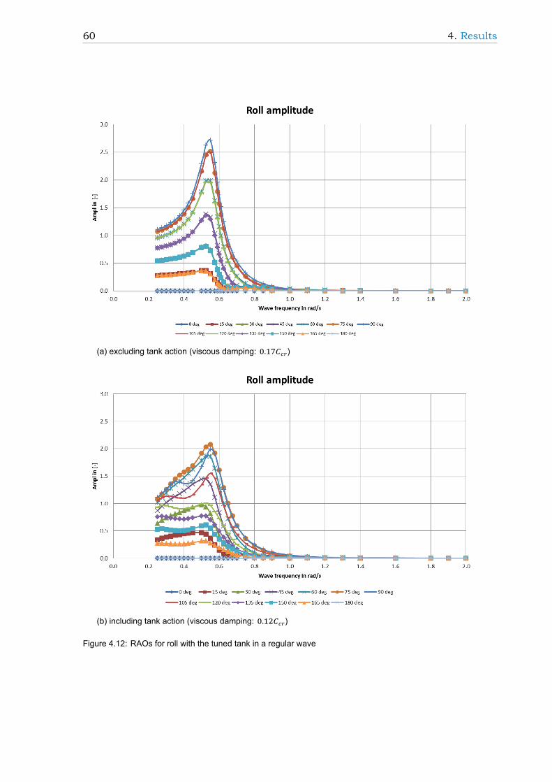
60 4. Results

(a) excluding tank action (viscous damping: . )

(b) including tank action (viscous damping: . )

Figure 4.12: RAOs for roll with the tuned tank in a regular wave

4.2. Frequency domain 61

Figure 4.13: Overdamped RAOs for roll with the tuned tank in a regular wave ( . )

Coupling of the tank action into othermotions Webster [9] stipulated that the free-floodingtanks influenced the roll motion in particular and had a small effect on the sway and yawmotions, whilst not having a significant effect on the heave and pitch motions. These effectsare found to be slightly different in the results as presented in appendix D. The anti-roll tankseems to have no significant effect on the surge, sway and yaw motions, while the heave andpitch motions are slightly influenced. These last two are a result of the heave force and pitchmoment of the tank. The influence is small and may be neglected. For the Jascon 18 thereis no coupling of the sway and yaw motions with the roll motions. Away from resonance theanti-roll tanks seem to have no effect on any of the motions.

4.2.2. Irregular wave responseIn this section only the results are shown for the motion of interest: roll. The amount ofadded damping is estimated here using Ikeda’s Method for Rectangular Barges [18] and thesignificant wave height in irregular waves. The value for the viscous damping of the roll motionfor this particular ship is iteratively determined to be 12% of the critical damping in an irregularJONSWAP wave spectrum with a significant wave height of 2.5 meters.

The expected response of the ship is given in figure 4.14b; the roll motion is reduced froman amplitude of 6.7 degrees to 4.7 degrees, which is a reduction of 30%.

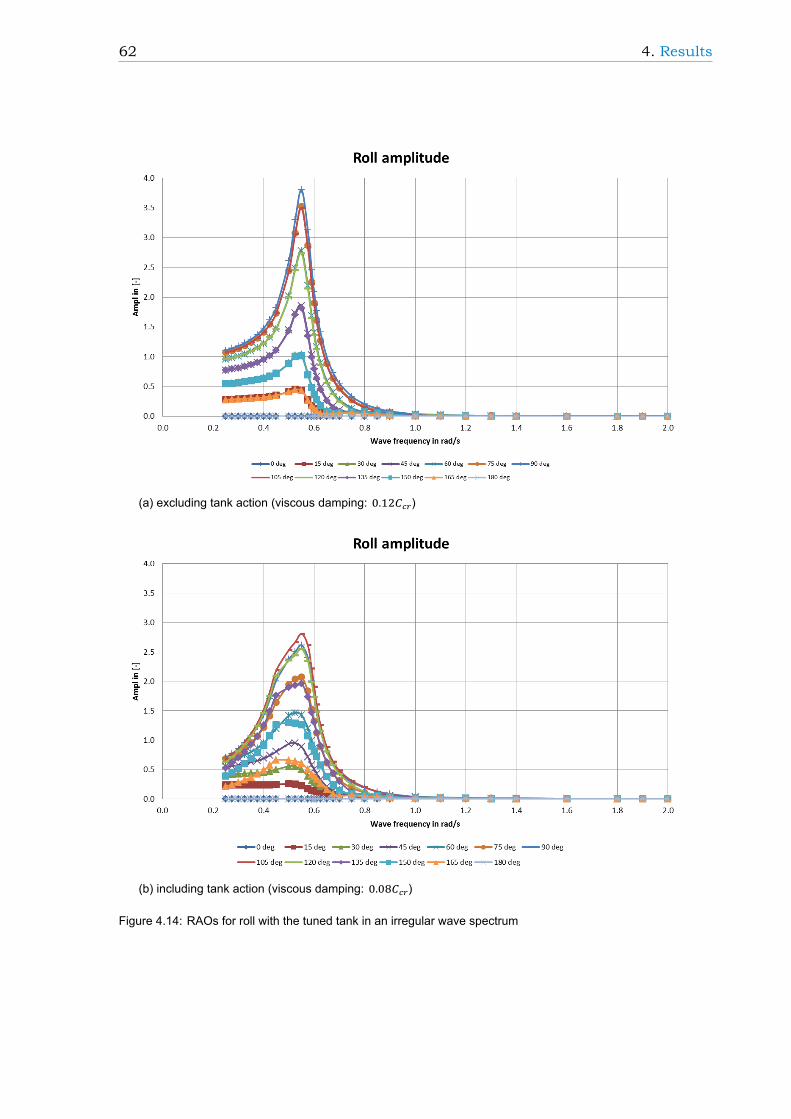
62 4. Results

(a) excluding tank action (viscous damping: . )

(b) including tank action (viscous damping: . )

Figure 4.14: RAOs for roll with the tuned tank in an irregular wave spectrum

4.3. Discussion of results 63

4.3. Discussion of resultsThe results are in a regular wave with an amplitude of 1 meter and beam seas condition (wavecoming in from starboard at 90∘ in the model).

4.3.1. Linearization of modelWebster in effect linearizes the mathematical model by computing the system of equations ina non-dimensional format (per one meter wave amplitude). However, if the model is computedwithout dividing through the wave height the tank performance is clearly non-linear with respectto wave height, as can be seen in figure 4.15. It is inversely and non-linearly related to waveheight and not linearly increasing. The shape of the curve is the same as found for the dampingcurve derived from the free decay analysis in § 4.1.1. This means that the RAOs given in§ 4.2 are only valid for a wave amplitude of one meter. Because of this result all the tankperformances given in this chapter are based on actual peak roll angles for a wave amplitudeof one meter and not on the RAO peak.

Figure 4.15: Tank performance for different wave heights

4.3.2. Comparison of simulation typesThe simulations are compared for a tuned tank with a flooding port size ratio of 0.22 to the freesurface area. The original roll peak is 4.8 deg.

The results from the frequency domain simulation and the direct time domain simulationscorrespond to each other. Even for the direct AQWA-NAUT simulation, even though, thereturned water levels are incorrect. Compared to the reduction in the direct AQWA-NAUTand SCILAB wave excited simulations the equivalent damping seems to underestimate thedamping of the roll motion by the free-flooding tanks only slightly. Nevertheless, indirectAQWA-NAUT simulation is really only useful if the roll angle data from the actual free decaytest of the ship is available, because that includes the viscous damping.

64 4. Results

Figure 4.16: Comparison of time and frequency domain simulation results

4.3.3. Comparison of Webster Model with VER ModelIn this section several tank designs are evaluated and compared to the results from the studyby VER in 2009.

In the VER Model with external free-flooding tanks a roll amplitude reduction of 37% wasfound for a tank with 𝛾 = 1 and a flooding port size of 22% of the free surface area [2].The layout of the tank is shown in figure 4.17a. This external tank is moved to the inside forevaluation with the Webster Model. Due to this move the flooding port is transferred from thebottom of the tank to the side.

(a) External free-flooding tank usedin the VER Model

(b) Internal free-flooding tank usedin the Webster Model

Figure 4.17: The tanks used for comparison of modeling

4.3. Discussion of results 65

The tank in the VERModel has an equilibrium water level of 2 meters. With this equilibriumwater level the inlet duct for a tuned tank needs to be unrealistically small to fit a geometryfactor of 16 plus the flooding port starts ventilating, which is not included in the model. In realitythe tuned tank needs more space under water to incorporate the shaping of the inlet duct plusa straight section under the free surface, so the tank performance of the tuned tank cannot beevaluated for an equilibrium water level of 2 meters.

The external water pressure head for the simulations is approximated using the waveelevation, because the potentials at the higher located flooding port were not available at thetime (i.e. no radiation pressure included in the Webster Model). The tank with 𝑑 = 2 showsthe best performance, however it should be noted that this tank will start ventilating at a staticroll angle of 7 degrees. For this or larger angles the tank effectiveness will decrease. Thetank performance is higher than that of the tank with a lower set flooding port (figure 4.16) asa result of the higher external pressure from the wave elevation. The wave elevation at theflooding port decreases as it is set lower in the hull (increasing 𝑑 ).

In the VERModel the roll reduction was estimated to be 37% for externally added free-floodinganti-roll tanks, in the Webster Model the internal free-flooding tanks are expected to damp theroll motion with 32%. One of the differences is that in the VER calculations steady flow isassumed, whilst Webster assumes quasi-steady flow. It was found that including the unsteadyterms (�� and �� ) in the model reduces the expected tank moment. The other differencebetween the models is the modeling of the pressure head at the flooding port: Froude Krylovhead plus velocity head versus wave elevation. Compared to the VERModel the tank performanceis estimated to be about 5% lower. Since there is no experiment data available, it is notpossible to conclude which of the twomodels gives a better estimation of the tank performance,but it is plausible that the Webster Model comes closer because it takes unsteady behavior ofthe tank water into consideration.

4.3.4. Comparison of air configurationsThe results in the fully vented, the separately vented and the crossover connected case areessentially equal, figure 4.18. The choice between the three configurations can therefore bebased entirely upon construction considerations, since air vent size has a nearly negligibleeffect on the performance of the tanks (also see figure 4.27).

The unvented tank can be considered a fully vented tank if the height of the plenum issufficiently large. As the height of the plenum is reduced, the roll reduction goes to zero. For aplenum height 𝑑 of 0.7 meters the roll reduction is a mere 0.5%. It is advantageous thereforeto minimize the height of the plenum and install an air vent with a valve in order to close offthe tank effectively turning it into an unvented tank. This way the tanks can be shut off. Fullyvented the water level comes up to 0.6 meters in the simulation, so the plenum height cannotbe reduced much further than 0.7 meters.

66 4. Results

Figure 4.18: Comparison of frequency domain results for different air configurations

It can be concluded that only for greatly restricted air flow or a small plenum height thereis an effect of air pressure on the tank water level, else the effect is so small that it might aswell be neglected. This is in line with the conclusions drawn by Webster who stated that thepart of the theory describing the effects of air pressure might as well not have been presenteven though it yields reasonable results compared for the physical model.

4.3.5. Influence of radiation pressureThe expectation was that the radiation pressure would have a larger influence on the tankperformance for ship 2 than for the Jascon 18, because the motion of the second ship isdamped in addition with viscous damping. As can be seen in figure 4.19 the radiation pressurehead has less influence on the tank performance of ship 2 (6%) than on the Jascon 18 (14%).However, the order of magnitude remains the same, so it is permissible to neglect radiationpressure if no data is available. This entails that the free surface height from AQWA may beused as input in the model if the potentials are unavailable.

Figure 4.19: Influence of pressure head components on tank performance

4.3. Discussion of results 67

4.3.6. Influence of tank parameters on tank performanceThe tank parameters are determined in the design stage and cannot be readily adapted oncethe tank has been built. This means that in the design stage a good deal of thought needs tobe put into working conditions and loading conditions.

On the subject of the design of the tank the conclusions of the influence of tank parametersare the following. Even though for this particular ship there seems to be no advantage of thetuned tank over the untuned tank, the tank performance can be optimized by thorough inletdesign. The flooding port size and duct shape have a great influence the tank transfer periodand the effective discharge coefficient.

Tank transfer periodThe tank transfer period is sensitive to the geometry factor and the equilibrium water level(figure 4.20). The tank transfer period can be adjusted by changing the equilibrium waterheight in the tank, for example by adjusting the location of the flooding port, or the geometryfactor by tuning. If the tanks would be actively controlled, the tank transfer period could alsobe adapted by changing the air pressure in the tanks, effectively changing 𝑑 . Adapting thetank transfer period does not alter the magnitude of the water level much, but does influencethe phase shift, positioning the tank moment more or less favorably with respect to the heelingmoment. Figure 4.21 shows that the tank moment for the tuned tank lags with 90∘ when thewave excitation period is equal to the ship natural roll period, at this point the tank will dampthe roll motion the most. For this particular ship the difference in tank performance is smalleven though the tank transfer period is heavily influenced, because the difference in phaselag between the untuned tank and the tuned tank is small (see figure 4.22).

-70%

-60%

-50%

-40%

-30%

-20%

-10%

0%

10%

20%

30%

40%

0 1 2 3 4 5 6 7 8 9 10

chan

ge in

tan

k tr

ansf

er

pe

rio

d [

%]

dw [m] / γ [-]

dw

γ

Figure 4.20: Influence of and on the tank transfer period

68 4. Results

(a) (b)

Figure 4.21: Tank moment amplitude and phase

(a) Influence of equilibrium water height

(b) Influence of tank geometry factor

Figure 4.22: Influence of tank transfer period on tank performance

For the aircraft carrier studied by Webster the theoretical difference in performance wassignificant. The performance difference between an untuned and a tuned tank is probablydependent on the location of the roll peak relative the location of the maximum wave potential

4.3. Discussion of results 69

damping. The wave potential damping for the aircraft carrier is presumably lower as its naturalroll period lies higher at 15.7 seconds versus 11.3 seconds for the Jascon 18. It must also benoted that the maximum roll angle of the aircraft carrier is likely much larger than the maximumroll angle of the Jascon 18 as its metacentric height is only half as high. The last has amaximum roll angle of only 4.8 degrees, which means that a round off error has a muchgreater influence on the results. In conclusion, for the Jascon 18 tuning has a small effect, butno general conclusion can be drawn on whether tuning for other vessels is necessary in orderto optimize performance.

Free surface area

Figure 4.23 shows a linear association of the tank free surface area with the tank performance.This means that if the performance is calculated for only two area sizes a good estimation canbe given. The maximum free surface area depends on the space available in the ship. Thechange in free-surface effect has not been taken into account in this influence evaluation.

Figure 4.23: Influence of free surface area on tank performance

Inlet coefficients

The non-dimensional flooding port size 𝛽 (figure 4.24) influences the flow rate and thus directlythe attained water level. Although it is treated separately here, it is linked to the tank geometryfactor, see equation (3.5): 𝐴(𝑠 = 0) = 𝛽𝐴 .The relationship between the flooding port size andtank performance is non-linear. The increase in tank performance levels off as the size of theflooding port increases. This effect is more pronounced with the lower viscous damping asused for the evaluation of the tank performance in irregular waves. Any construction issueshave not been taken into account, but in the design a trade off between pipe design, tankgeometry factor and flooding port size exists.

The effective discharge coefficient 𝐶 (figure 4.25) influences the roll damping less stronglythan the flooding port size, but still significantly. The parameter depends on the size of theflooding port and the shape of the duct behind it. For the untuned tank the discharge coefficientis more or less constant, but the effectiveness of the tuned tank can be optimized through the

70 4. Results

inlet design. The determination of this coefficient is treated more extensively in the introductionof this chapter where the choice for the tank parameters in this report is elaborated upon.

Figure 4.24: Influence of flooding port size on performance

Figure 4.25: Influence of flooding port discharge coefficient on water level

Air vent coefficientsThe vent coefficients 𝛼 (dimensionless vent size) and 𝐶 (air discharge coefficient) of courseonly play a role in the case of separate venting and not in the fully vented case. The comparisongiven in this paragraph cannot entirely be justified, because the air discharge coefficient dependsto a large extent on the vent size. Unfortunately, since the Webster Model does use the twocoefficients separately, they need to be defined independently in order to get a result.

Despite of the interdependency of the vent size and the discharge coefficient an attemptis made here to at least give a quantitative indication of the effect of the vent size 𝛼. The sizeof the vent has a significant influence on the water level up to about 1.5% of the free surface

4.3. Discussion of results 71

area with the air discharge coefficient set at 0.7; for larger vent sizes the behavior will not differfrom the fully vented case (𝛼 = 1).

The air discharge coefficient is found to vary between 0.19 and 1.25 according to Kinsman [21]and these limits are also held here. It seems that the value chosen by Webster (0.7) lies in themiddle of the range and should be a safe estimated value for the effective discharge coefficient.

(a) dimensionless size of vent (b) air discharge coefficient

Figure 4.26: Influence of air coefficients on tank performance

From figure 4.27 it is clear that the effect of the air pressure on the tank water level isminimal unless the lower limit is approached, where uncertainties in the correctness of thevalues are large. This means that, unless 𝛼𝐶 is very small, exact values for the ventcoefficients are not important to obtain a good indication of tank water level and the generatedtank moment. This is in line with the conclusion that there is a negligible effect of passive airpressure on the tank performance. It is adequate to use estimated values in the tank model.In combination with the results in figure 4.18 it can be said that the design of air vents issecondary to the design of the water inlet.

Figure 4.27: Influence of combined air vent coefficients on tank performance

5Conclusions and recommendations

5.1. ConclusionsA roll reduction of 30% may be expected in irregular waves for this particular vessel for a peakroll angle of 6.7 degrees in beam seas. This maximum roll angle is small, which means thatthe uncertainty in the tank performance is relatively large.

The tank performance is non-linearly related to the differential pressure head over theflooding port and therewith directly with the incoming wave height. Consequently the shipresponse should not be defined using RAOs, but using the actual predicted roll angle.

The tank performance for the frequency domain and time domain simulations in SCILABagree as essentially the system of equations is solved in the same way. If the radiationpressure is not taken into account the tank performance can differ with a few percent from thetank performance calculated including the radiation pressure, however, the order of magnituderemains the same. This means that the wave elevation at the flooding port from AQWA(Froude-Krylov plus diffraction) obtains sufficient information on the pressure head to givea good indication of the tank performance.

For a time simulation the equations of motion and tank equation should be integratedsimultaneously and interactively. In the AQWA-NAUT time simulation this is not possibleand results are considered unreliable. An indirect time simulation in AQWA-NAUT using tankdamping values from a theoretical free decay analysis differs significantly from the estimatedtank performance by SCILAB. It is possibly a good alternative if experimental values from afree decay test of the actual ship are available.

The parameters influencing tank performance are identified for design purposes. Eventhough for this particular ship there seems to be no advantage of the tuned tank over theuntuned tank, the tank performance can be optimized by thorough inlet design. The floodingport size and duct shape have a great influence the tank transfer period and the effectivedischarge coefficient. Fitting a valve on the air vent or in the crossover connection between thetanks enables a shutdown of the tanks, if the height of the tank above equilibrium water level is

73

74 Bibliography

sufficiently small. Otherwise the air pressure has a negligible effect on the tank performanceand the most convenient configuration for construction may be selected.

5.2. RecommendationsThe coupled ship and tank model explored in this report has been verified as far as feasible.To validate these calculations it is advised to perform experiments. Webster found a goodcorrelation between the model and experiments.

Design aspects have not been taken into consideration in this report, while they are essentialfor the determination of the expected tank performance. One of the important aspects lackingin the results is a good estimate of the effective discharge coefficient for the tuned tank.

The SCILAB time domain simulation presented in this report simply solves the equationsof motion and the tank equation separately at each time step. If more extensive calculationsin time domain are desired, it is advisable to at least include the influence of the motions fromthe previous time intervals (”memory”) plus retardation functions. It might also be of interestto include a non-linear restoring and damping moment to closer approximate the roll behaviorof the ship.

A possible improvement on the frequency domain simulation is a multi-domain simulationwhere the interaction between the tank and the ship directly depend on each other. Thedifferential pressure head over the flooding port can then be determined directly at the jointboundary of the domains.

Bibliography

[1] Free-flooding Anti-roll Tanks - feasibility study, Tech. Rep. 09.185 R01 - Rev B1 (VuykEngineering Rotterdam B.V., 2010).

[2] Free-flooding Anti-roll Tanks - preliminary tank dimensions, Tech. Rep. 09.185 R02 - RevB (Vuyk Engineering Rotterdam B.V., 2010).

[3] J. H. Chadwick,On the stabilization of roll, Transactions - Society of Naval Architects andMarine Engineers (SNAME) 63, 237 (1955).

[4] Anti Roll Tank System for Offshore Crane/Pipelay Vessel - phase 1, Tech. Rep. 24001-100(Maritime Research Instistute Netherlands (MARIN), 2010).

[5] Anti Roll Tank System for Offshore Crane/Pipelay Vessel - phase 2, Tech. Rep. 24001-300(Maritime Research Instistute Netherlands (MARIN), 2010).

[6] AQWA-LINE User Manual, ANSYS, Inc., release 14.5 ed. (2012).

[7] AQWA-NAUT User Manual, ANSYS, Inc., release 14.5 ed. (2012).

[8] Wikipedia, the free encyclopedia (2014).

[9] W. C. Webster, J. F. Dalzell, and R. A. Barr, Prediction and measurement of theperformance of free-flooding ship antirolling tanks, Transactions - Society of NavalArchitects and Marine Engineers (SNAME) 96, 333 (1988).

[10] J. A. Pinkster, Low Frequency Second Order Wave Exciting Forces on FloatingStructures, Ph.D. thesis, Delft University of Technology (1980).

[11] H. Rouse, Elementary Mechanics of Fluids (Wiley, New York, 1946).

[12] C. Stigter, Performance of U-Tanks as a Passive Anti-Rolling Device, Tech. Rep. reportno. 81S (Delft Hydraulics Laboratory, TNO, 1966).

[13] R. A. Barr and V. Ankudinov, Ship rolling, its prediction and reduction using rollstabilization, Marine Technology 14, 19 (1977).

[14] J. D. Skufca, Analysis still matters: A surprising instance of failure ofRunge–Kutta–Felberg ODE solvers, SIAM review 46, 729 (2004).

75

76 Bibliography

[15] J. R. Cash and A. H. Karp, A variable order Runge-Kutta method for initial value problemswith rapidly varying right-hand sides, ACM Trans. Math. Softw. 16, 201 (1990).

[16] S. N. Blagoveshchensky, Theory of Ship Motions, edited by L. Landweber, Vol. 2 (DoverPublications, New York, 1962) translated from the 1st Russian edition by T. Strelkoff andI. Strelkoff.

[17] P. D. Chaplin, The effectiveness of roll stabilisers, The Naval Architect 2, 33 (1972).

[18] Y. Ikeda, T. Fujiwara, and T. Katayama, Roll damping of a sharp-cornered barge androll control by a new-type stabilizer, in Proceedings of the 3rd International Offshore andPolar Engineering Conference (1993) pp. 634–639.

[19] P. Ruponen, Progressive Flooding of a Damaged Passenger Ship, Ph.D. thesis, HelsinkiUniversity of Technology, Espoo, Finland (2007).

[20] IMO Resolution A.266(VIII) SLF50/10, (2007).

[21] R. G. Kinsman,Outlet Discharge Coefficients of Ventilation Ducts, Master’s thesis, McGillUniversity, Montreal (1990).

[22] W. H. Press, S. A. Teukolsky, W. T. Vetterling, and B. P. Flannery, Numerical Recipesin C++: The art of scientific computing, 2nd ed. (Cambridge University Press, New York,2002).

ADynamic air pressure

Substituting the atmospheric pressure 𝑅 , the linearized discharge coefficient 𝑅 and thestandard atmospheric conditions 𝑅 into equation (3.10), the mass flow becomes:

�� = 𝛼𝐴 ⋅ 𝐶 √𝑝

|𝑝 − 𝑝 | ⋅ √|𝑝 − 𝑝 |

𝑝 ⋅ √2𝜌 (𝑝 − 𝑝 ) = 𝛼𝐴 𝑅 √2𝜌𝑝 (𝑝 − 𝑝 )

= 𝛼𝐴 𝑅 √2𝜌𝑝 (𝑝 − 𝑝 ) = 𝛼𝑅 𝑚

𝑑 𝑝 √2𝑝𝜌 (𝑝 − 𝑝 ) = 𝛼𝑅 𝑅 𝑚

𝑑 𝑝 (𝑝 − 𝑝 )

Net air mass Δ𝑚 extracted from the starboard tank is the integral over time of the mass flow:

𝑝 Δ𝑚𝑚 = 𝛼𝑅 𝑅

𝑑 ∫ (𝑝 − 𝑝 )𝑑𝑡 (A.1)

The mass density is:

𝜌 = 𝑀 − Δ𝑀𝐴 (𝑑 − Υ ) = 𝜌

1 − Δ𝑀/𝑀1 − Υ/𝑑

Linearize this mass density around 𝑎 = 0. The general formula for linearizion is 𝐿(𝑥) = 𝑓(𝑎)+𝑓 (𝑎)(𝑥 − 𝑎).

𝑥 = Δ𝑀𝑀

𝑓(𝑥) = 1 − 𝑥 ⇒ 𝑓(0) = 1𝑓 (𝑥) = −1 ⇒ 𝑓 (0) = −1

𝐿 (𝑥) = 1 + (−1) ⋅ (𝑥 − 0) = 1 − 𝑥 = 1 − Δ𝑀𝑀

77

78 A. Dynamic air pressure

𝑥 =Υ𝑑

𝑓(𝑥) = 11 − 𝑥 ⇒ 𝑓(0) = 1

𝑓 (𝑥) = 1(1 − 𝑥) ⇒ 𝑓 (0) = 1

𝐿 (𝑥) = 1 + 1 ⋅ (𝑥 − 0) = 1 + 𝑥 = 1 +Υ𝑑

𝐿(𝑥) = 𝐿 (𝑥) ⋅ 𝐿 (𝑥) = (1 − Δ𝑀𝑀 )(1 +Υ𝑑 ) = 1 − Δ𝑀𝑀 +

Υ𝑑 − Δ𝑀𝑀 ⋅

Υ𝑑

𝜌 = 𝜌 (1 − Δ𝑀𝑀 +Υ𝑑 ) ⇒ 𝑝 = 𝑝 (1 − Δ𝑀𝑀 +

Υ𝑑 )

Δ𝑀𝑀 = 1 +

Υ𝑑 −

𝑝𝑝 (A.2)

Substitute (A.2) into (A.1) and convert the air pressures into equivalent water heads:

Δ𝑀𝑀 𝑝 = (1 +

Υ𝑑 −

𝑝𝑝 )𝑝 = 𝑝 − 𝑝 +

Υ 𝑝𝑑

= 𝛼𝑅 𝑅𝑑 ∫ (𝑝 − 𝑝 )𝑑𝑡

𝑝 − 𝑝 =Υ 𝑝𝑑 − 𝛼𝑅 𝑅

𝑑 ∫ (𝑝 − 𝑝 )𝑑𝑡

𝑝 − 𝑝𝜌𝑔 =

Υ𝑑𝑝𝜌𝑔 −

𝛼𝑅 𝑅𝑑 ∫ (

𝑝 − 𝑝𝜌𝑔 −

𝑝 − 𝑝𝜌𝑔 ) 𝑑𝑡

Substituting 𝑃 = and 𝑅 = in the above air pressure equation for simplicity, resultsin:

𝑃 = 𝑅𝑑 Υ − 𝛼𝑅 𝑅

𝑑 ∫ (𝑃 − 𝑃 )𝑑𝑡

𝑃 + 𝛼𝑅 𝑅𝑑 ∫ 𝑃 𝑑𝑡 = 𝑅

𝑑 Υ − 𝛼𝑅 𝑅𝑑 ∫ 𝑃 𝑑𝑡

with the newly defined atmospheric pressure in head of water 𝑅 = . As an example, theair pressure head is derived for separate venting. Since the tanks are not interconnected in

79

the separate venting case, the coupled air pressure term 𝑃 drops out:

𝑃 = 𝑅𝑑 Υ + 𝑖 ⋅ 𝛼𝑅 𝑅

𝑑 ⋅ 𝑃𝜔

(1 − 𝑖 ⋅ 𝛼𝑅 𝑅𝜔 𝑑 )𝑃 = 𝑅

𝑑 Υ

𝜔 𝑑 − 𝑖𝛼𝑅 𝑅𝜔 𝑑 ⋅ 𝑃 = 𝑅

𝑑 Υ

𝑃 = 𝑅𝑑 Υ ⋅ 𝜔 𝑑

𝜔 𝑑 − 𝑖𝛼𝑅 𝑅 ⋅ 𝜔 𝑑 + 𝑖𝛼𝑅 𝑅𝜔 𝑑 + 𝑖𝛼𝑅 𝑅

= 𝑅𝑑 ⋅ 𝜔 𝑑 + 𝑖𝜔𝑑 𝛼𝑅 𝑅

𝜔 𝑑 + 𝛼 𝑅 𝑅 ⋅ Υ

= 𝜔 𝑅 𝑑 + 𝑖𝜔𝛼𝑅 𝑅 𝑅𝜔 𝑑 + 𝛼 𝑅 𝑅 ⋅ Υ = 𝑉Υ

If the coupled air pressure term does not drop out, equation (3.11) (applying linear assumptions)reduces to:

𝑃 = 𝑉 Υ + 𝑈Υ

BNumerical methods

The two numerical methods (Runge-Kutta and Cash-Karp), which were found to be the mostsuitable for computing the time domain problem in § 3.3.2, are described in this appendixsection.

B.1. Fixed step method (Runge-Kutta)A numerical method is an iterative method for the approximation of the solution of an ordinarydifferential equation. One of many numerical methods is the explicit recursive Runge-Kuttamethod (often abbreviated to RK4). This method is first order, which means that a secondorder differential equation needs to be simplified to contain only first derivatives in order to beable to implement the RK4 method. The initial value problem should be specified as follows:

�� = 𝑓(𝑡, 𝑥), 𝑥(𝑡 ) = 𝑥

From this initial value vector 𝑥 the approximation of 𝑥(𝑡 ) is calculated at a brief time later(𝑡 = 𝑡 + ℎ, where ℎ is the step size) by adding the weighted average of four incrementsto the value at the present time 𝑥 :

𝑡 = 𝑡 + ℎ

𝑥 = 𝑥 + ℎ (16𝑘 + 13𝑘 + 13𝑘 + 16𝑘 )

𝑘 = 𝑓(𝑡 , 𝑥 )

𝑘 = 𝑓 (𝑡 + ℎ2 , 𝑥 + ℎ2𝑘 )

𝑘 = 𝑓 (𝑡 + ℎ2 , 𝑥 + ℎ2𝑘 )

𝑘 = 𝑓 (𝑡 + ℎ, 𝑥 + ℎ𝑘 )

where 𝑥 is the approximation of 𝑥(𝑡 ). The 𝑘 -terms are estimated slopes of the functionat the specified time. Multiplied with the size of the interval this gives an increment to the value

81

82 B. Numerical methods

at the present time. Basically, the RK4 method takes a trial step to the midpoint of the timeinterval twice and then uses the values at both the beginning and the midpoint to compute the“real” step across the whole interval.

In the implementation of the method in the calculations the generalized form of the RK4 isused. It is given by:

𝑥 = 𝑥 + ℎ∑𝑏 𝑘

𝑘 = 𝑓(𝑡 + 𝑐 ℎ, 𝑥 + ℎ∑𝑎 𝑘 )

= 1𝐶 ([

0 𝐶−1 −𝐶 |𝑦 + ℎ∑ 𝑎 𝑘 | |

] 𝑥 − [ 0𝐶] 𝑍 + [0

1]𝐻 )

The coefficients 𝑎, 𝑏 and 𝑐 can be arranged in a schematic called the Butcher tableau:

𝑐 𝑎 𝑎 𝑎 𝑎

=

0 0 0 0 0𝑐 𝑎 𝑎 𝑎 𝑎 1/2 1/2 0 0 0𝑐 𝑎 𝑎 𝑎 𝑎 1/2 0 1/2 0 0𝑐 𝑎 𝑎 𝑎 𝑎 1 0 0 1 0

𝑏 𝑏 𝑏 𝑏 1/6 1/3 1/3 1/6

For the first order system of equations as given in equation (3.13) the Runge-Kutta algorithmremains unchanged, the variables are simply replaced by vectors.

B.2. Variable step method (Cash-Karp)The Cash-Karp method is an extended Runge-Kutta method and thus structured and solved inthe same way. The difference is that both a fourth and fifth order method are used to estimatethe truncation error at each time step. This truncation error is compared to a desired maximumerror Δ . If the truncation error is larger than the desired error the calculation step is repeatedwith a smaller step size until the error condition is met. The solution is then set to the fifth orderapproximation and the next time step is then initiated. The implementation of the varying stepsize has been taken from Press [22]. The Butcher tableau for the Cash-Karp method is:

0 01/5 1/5 03/10 3/40 9/40 03/5 3/10 -9/10 6/5 01 -11/54 5/2 -70/27 35/27 07/8 1631/55296 175/512 575/13824 44275/110592 253/4096 0

37/378 0 250/621 125/594 0 512/17712825/27648 0 18575/48384 13525/55296 277/14336 1/4

B.2. Variable step method (Cash-Karp) 83

The first row of the 𝑏-coefficients is the fourth order approximation to the system (𝑏∗) and thesecond row the fifth order approximation (𝑏 ). The difference between the two (local error) canbe described with:

Δ =∑(𝑏 − 𝑏∗)𝑘

For the simulations other than the test case a desiredmaximum error, relative to the dependentvariables and the system of equations, is defined in order to keep the factional errors constant.

Δ = 𝑚𝑎𝑥 [𝑒𝑝𝑠 (|𝑥| + |ℎ ��|)]

where 𝑒𝑝𝑠 is the overall tolerance level. The recommended time step for the next calculationstep is:

ℎ =⎧⎪⎨⎪⎩

0.9ℎ | |.

0.9ℎ | |.

Δ ≥ Δ

Δ < Δ

It is advisable to put in a safety factor of 0.9 in the step size change, because the estimatesof error are only indicative and not exact.

CTheory of decay analysis

85

86 C. Theory of decay analysis

From the recorded decay curves of the various decay/free extinction tests the damping

coefficients may be derived from the decrease of motion amplitude for two successive

oscillations. Also the natural periods may be derived from the tests.

x(t) = time history of motion x

xan = motion amplitude of n-th oscillation

T� = natural period of motion x.

If the motion x(t) during a free extinction test is described by:

0 = x . c + |x| . x . b + x . b + x . a x(2)x

(1)xx ✁✁✁✁✁

where:

ax = total mass (ship mass + added mass) in mode x

b(1)x = linear damping coefficient in mode x

b(2)x = quadratic damping coefficient in mode x

cx = restoring coefficient in mode x

the linear and quadratic damping coefficients are found in the following way:

When the decrease of motion amplitude divided by the mean motion amplitude is plotted

versus the mean motion amplitude the damping coefficients are determined by:

..

87

Ta . p . 2 = b

x

x(1)x (2)

xx3

b = . q . a8

In order to be able to determine the values p and q a line has been fitted through the data

points found from the decay tests.

The equivalent linearised damping at a particular amplitude xa follows from the effective

“p” value at that amplitude according:

gGMT

cab xxxCR ....

2

)x . q + (p..2.

2

)x . q + (p = .

2

)x . q + (p = b

aaax �✁

✂✂✂✂

In the above Tx denotes the roll period and GM.✄.g the restoring term in roll (the product of

transverse GM and displacement weight ✄.g in kN).

..

DRAOs for all motion directions

89

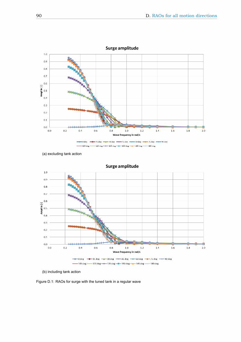
90 D. RAOs for all motion directions

(a) excluding tank action

(b) including tank action

Figure D.1: RAOs for surge with the tuned tank in a regular wave

91

(a) excluding tank action

(b) including tank action

Figure D.2: RAOs for sway with the tuned tank in a regular wave

92 D. RAOs for all motion directions

(a) excluding tank action

(b) including tank action

Figure D.3: RAOs for heave with the tuned tank in a regular wave

93

(a) excluding tank action

(b) including tank action

Figure D.4: RAOs for roll with the tuned tank in a regular wave

94 D. RAOs for all motion directions

(a) excluding tank action

(b) including tank action

Figure D.5: RAOs for pitch with the tuned tank in a regular wave

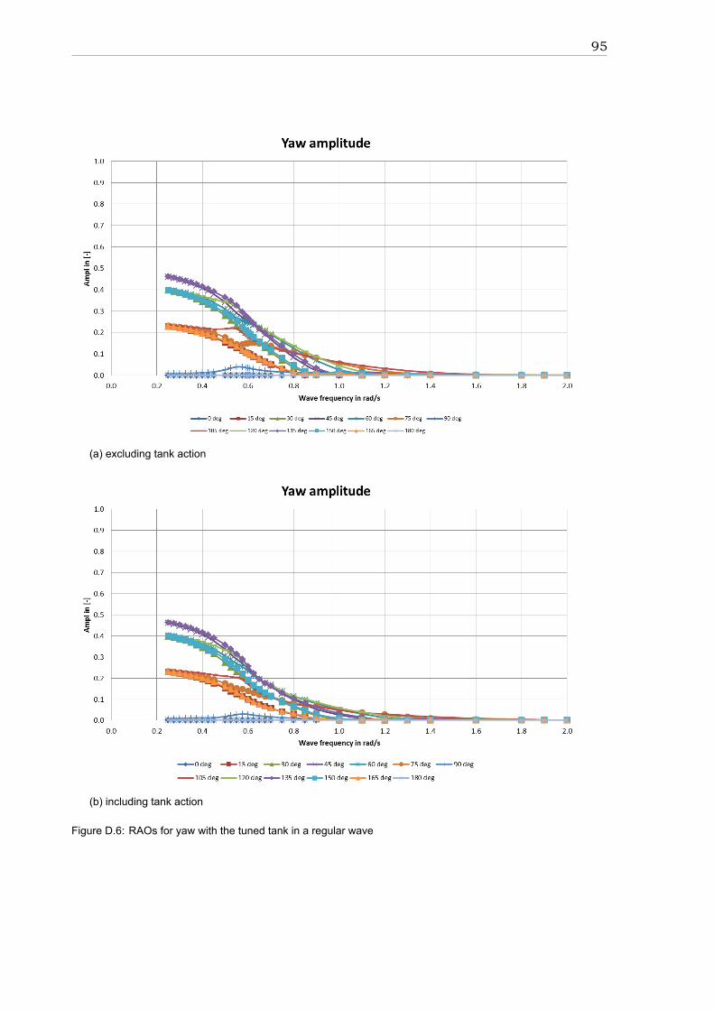
95

(a) excluding tank action

(b) including tank action

Figure D.6: RAOs for yaw with the tuned tank in a regular wave