Mathematical Modeling of T-Cell Experimental Data · Prof. M. Hasler, président du jury Prof....
134
POUR L'OBTENTION DU GRADE DE DOCTEUR ÈS SCIENCES acceptée sur proposition du jury: Prof. M. Hasler, président du jury Prof. J.-Y. Le Boudec, directeur de thèse Prof. R. J. de Boer, rapporteur Dr C. Kohl, rapporteur Prof. J.-P. Kraehenbuehl, rapporteur Mathematical Modeling of T-Cell Experimental Data THÈSE N O 4881 (2010) ÉCOLE POLYTECHNIQUE FÉDÉRALE DE LAUSANNE PRÉSENTÉE LE 19 NOVEMBRE 2010 À LA FACULTÉ INFORMATIQUE ET COMMUNICATIONS LABORATOIRE POUR LES COMMUNICATIONS INFORMATIQUES ET LEURS APPLICATIONS 2 PROGRAMME DOCTORAL EN INFORMATIQUE, COMMUNICATIONS ET INFORMATION Suisse 2010 PAR Irina BALTCHEVA
Transcript of Mathematical Modeling of T-Cell Experimental Data · Prof. M. Hasler, président du jury Prof....

POUR L'OBTENTION DU GRADE DE DOCTEUR ÈS SCIENCES
acceptée sur proposition du jury:
Prof. M. Hasler, président du juryProf. J.-Y. Le Boudec, directeur de thèse
Prof. R. J. de Boer, rapporteur Dr C. Kohl, rapporteur
Prof. J.-P. Kraehenbuehl, rapporteur
Mathematical Modeling of T-Cell Experimental Data
THÈSE NO 4881 (2010)
ÉCOLE POLYTECHNIQUE FÉDÉRALE DE LAUSANNE
PRÉSENTÉE LE 19 NOVEMBRE 2010
À LA FACULTÉ INFORMATIQUE ET COMMUNICATIONS
LABORATOIRE POUR LES COMMUNICATIONS INFORMATIQUES ET LEURS APPLICATIONS 2
PROGRAMME DOCTORAL EN INFORMATIQUE, COMMUNICATIONS ET INFORMATION
Suisse2010
PAR
Irina BALTCHEVA


Abstract
T lymphocytes (T cells) are key components of the adaptive immune system. These cellsare able to recognize an enormous variety of pathogens thanks to the great specificity of theirtrans-membrane proteins, the T cell receptors (TCRs). TCR diversity is created during T cellmaturation in the thymus by somatic gene-segment rearrangements and random nucleotide ad-ditions or deletions. Out of all possible T cell clones bearing specific TCRs, only a small frac-tion are successfully released in peripheral blood as the result of clonal selection. Among theselected clones, some self-reactive cells with the capacity to induce an auto-immune disease areerroneously released in periphery. To compensate for this functional flaw, the immune systemhas developed peripheral control mechanisms. One of them are regulatory T cells that are spe-cialized in the control of harmful self-reactive clones. In this thesis, we combine mathematicalmodeling and experimental data to address immunological questions related to the dynamicsof regulatory T cells and to the measurement of the structural diversity of T cell receptors. Thedissertation is split into two main parts.
In the first part, we model the lifelong dynamics of human regulatory T cells (Tregs). De-spite their limited proliferation capacity, Tregs constitute a population maintained over the entirelifetime of an individual. The means by which Tregs sustain a stable pool in vivo are controver-sial. We define a novel mathematical model that we use to evaluate several biological scenariosabout the origins and the proliferation capacity of two subsets of Tregs: precursor CD4+CD25+-CD45RO− and mature CD4+CD25+CD45RO+ cells. The lifelong dynamics of Tregs are de-scribed by a set of ordinary differential equations, driven by a stochastic process representingthe major immune reactions involving these cells. Most of the parameters are considered asrandom variables having an a priori distribution. The likelihood of a scenario is estimated us-ing Monte Carlo simulations. The model dynamics are validated with data from human donorsof different ages. Analysis of the data led to the identification of two properties of the dynam-ics: (a) the equilibrium in the CD4+CD25+ Tregs population is maintained over both precursorand mature Tregs pools together, and (b) the ratio between precursor and mature Tregs is invertedin the early years of adulthood. Then, using the model, we identified four biologically relevantscenarios that have the above properties: (1) if the unique source of mature Tregs is the antigen-driven differentiation of precursors that acquire the mature profile in the periphery, then theproliferation of Tregs is essential for the development and the maintenance of the pool; if thereexist other sources of mature Tregs, such as (2) a homeostatic regulation, (3) a thymic migration,or (4) a peripheral conversion of effectors into Tregs, then the antigen-induced proliferation isnot necessary for the development of a stable pool of Tregs.
In the second part of the dissertation, we address the general question of TCR diversity by
i

improving the interpretation of AmpliCot, an experimental technique that aims at the diversitymeasurement of nucleic acid sequences. This procedure has the advantage over other cloningand sequencing techniques of being time- and expense- effective. In short, a fluorescent dyethat binds double-stranded DNA is added to a sample of PCR-amplified DNA. The sample ismelted, such that the DNA becomes single-stranded, and then re-annealed under stringent con-ditions. The annealing kinetics, measured in terms of fluorescence intensity, are a function ofthe diversity and of the concentration of the sample and have been interpreted assuming secondorder kinetics. Using mathematical modeling, we show that a more detailed model, involvingheteroduplex- and transient-duplex formation, leads to significantly better fits of experimentaldata. Moreover, the new model accounts for the diversity-dependent fluorescence loss that istypically observed. As a consequence, we show that the original method for interpreting the re-sults of AmpliCot experiments should be applied with caution. We suggest alternative methodsfor diversity extrapolation of a sample.
Keywords: Mathematical modeling, regulatory T cells (Tregs), T cell receptor (TCR) diver-sity, AmpliCot, ordinary differential equations, likelihood estimation.
ii

Résumé
Les lymphocytes T (cellules T) sont des éléments clés du système immunitaire adaptatif.Ces cellules reconnaissent une large variété de pathogènes grâce à la spécificité de leurs pro-téines trans-membranaires, les récepteurs des cellules T (TCR). La diversité des TCR est crééelors de la maturation des cellules T dans le thymus par des réarrangements de segments degènes et l’ajout ou la suppression aléatoire de nucléotides. Parmi tous les clonotypes possible-ment générés ainsi, seule une petite fraction est sélectionnée pour sortir du thymus et rejoindreles tissus périphériques en tant que population fonctionnelle. Cependant, parmi les clones sélec-tionnés, certaines cellules auto-réactives, ayant la capacité d’induire une maladie auto-immune,sont libérées dans la périphérie. Pour compenser cette faille fonctionnelle, le système immuni-taire a développé des mécanismes de contrôle périphérique dont font partie les lymphocytes Trégulateurs. Ces cellules sont en effet spécialisées dans le contrôle des clones autoréactifs pos-siblement nuisibles. Cette thèse combine la modélisation mathématique à des données expéri-mentales pour répondre à des questions immunologiques concernant la dynamique des cellulesT régulatrices et l’estimation de la diversité structurelle des TCR. La dissertation consiste endeux parties principales.
Premièrement, nous étudions la dynamique des cellules T régulatrices (Tregs). En dépit deleur capacité de prolifération limitée, ces dernières constituent une population qui persiste pen-dant toute la vie d’un organisme humain. Les mécanismes par lesquels les Tregs se renouvellentet maintiennent une réserve stable in vivo sont controversés. Nous définissons un modèle ma-thématique afin d’évaluer plusieurs scénarios biologiques concernant les origines et la capacitéde prolifération de deux sous-ensembles de Tregs : les cellules Tregs précurseurs (CD4+CD25+-CD45RO−) et matures (CD4+CD25+CD45RO+). La dynamique des Tregs est décrite par deséquations différentielles ordinaires couplées à un processus stochastique qui simule les réac-tions immunitaires majeures impliquant ces cellules. La majorité des paramètres est considéréealéatoire, ayant une distribution déterminée à priori (approche du type Bayesien). Le rapportde vraisemblance entre deux scénarios est estimé par des simulations Monte Carlo. Les trajec-toires du modèle sont validées par des données expérimentales provenant de donneurs humainssains de différents âges. L’analyse des données a permis l’identification de deux propriétés : (a)l’équilibre dans la population des Tregs opère sur les deux sous-populations de cellules précur-seurs et matures prises ensemble, et (b) le rapport entre les précurseurs et les Tregs matures estinversé au cours des premières années de l’âge adulte. À l’aide de notre modèle, nous avonsidentifié quatre scénarios biologiquement réalistes qui possèdent les propriétés précédentes :(1) si la seule source de Tregs matures est la différentiation engendrée par un stimulus antigé-nique des précurseurs dans les tissus périphériques, alors la prolifération des Tregs est essentielle
iii

au développement et au maintien de leur population ; s’il existe d’autres sources de Tregs ma-tures, telles que (2) la prolifération homéostatique, (3) la migration du thymus, ou (4) la trans-formation de cellules effectrices en Tregs, alors la prolifération en réponse à une stimulationantigénique n’est pas nécessaire au développement d’un bassin stable de Tregs.
Dans la deuxième partie de la thèse, nous abordons la question générale de la diversitédes TCR en améliorant l’interprétation d’AmpliCot, une technique expérimentale destinée àla mesure de la diversité des séquences d’acides nucléiques. Cette procédure présente l’avan-tage par rapport aux autres techniques de clonage et de séquençage d’être plus efficace entermes de coût et de temps. En bref, un colorant fluorescent, qui lie l’ADN double-brin, estajouté à un échantillon d’ADN amplifié par PCR. L’échantillon est fondu, de sorte que l’ADNdevient simple-brin, puis re-associé dans des conditions expérimentales strictes. La cinétiquede ré-association, mesurée en termes d’intensité de fluorescence, est une fonction de la diver-sité et de la concentration de l’échantillon. Elle a été interprétée en assumant une cinétiquedu second ordre. À l’aide de modélisation mathématique, nous montrons qu’un modèle plusdétaillé, comportant des hétéroduplexes et des complexes transitoires, reproduit de façon plusfidèle les données expérimentales. En outre, le nouveau modèle permet d’expliquer une pertede fluorescence généralement observée et qui est positivement corrélée à la diversité. En consé-quence, nous montrons que la méthode d’interprétation des résultats expérimentaux, suggéréeinitialement, devrait être appliquée avec prudence. Nous suggérons des méthodes alternativesd’extrapolation de la diversité d’un échantillon.
Mots clés : Modélisation mathématique, lymphocytes T régulateurs (Tregs), diversité des ré-cepteurs des cellules T (TCR), AmpliCot, équations différentielles ordinaires, estimateur devraisemblance.
iv

Contents
Abstract i
Résumé iii
List of Abbreviations ix
1 General Introduction 1
1.1 Adaptive Immunity: from Diversity to Self-Tolerance . . . . . . . . . . . . . . . 11.1.1 Generation of TCR diversity . . . . . . . . . . . . . . . . . . . . . . . . . 21.1.2 Clonal Selection . . . . . . . . . . . . . . . . . . . . . . . . . . . . . . . . 31.1.3 Regulatory T cells . . . . . . . . . . . . . . . . . . . . . . . . . . . . . . . 4
1.2 Mathematical Modeling in Immunology . . . . . . . . . . . . . . . . . . . . . . 51.3 Dissertation Outline . . . . . . . . . . . . . . . . . . . . . . . . . . . . . . . . . . 6
I Dynamics of Regulatory T cells 7
2 Lifelong Dynamics of Human CD4+CD25+ Regulatory T Cells 9
2.1 Introduction . . . . . . . . . . . . . . . . . . . . . . . . . . . . . . . . . . . . . . . 92.1.1 Mathematical Models of Tregs: State of the Art . . . . . . . . . . . . . . 10
Crossregulation Model of Immunity (Tregs and APCs) . . . . . . . . . . 11Tregs and APCs . . . . . . . . . . . . . . . . . . . . . . . . . . . . . . . . 12Tregs and Cytokine Kinetics . . . . . . . . . . . . . . . . . . . . . . . . . 13Adaptive/Induced Tregs . . . . . . . . . . . . . . . . . . . . . . . . . . . . 13Tregs and Gene Expression . . . . . . . . . . . . . . . . . . . . . . . . . . 14Tregs and Evolution . . . . . . . . . . . . . . . . . . . . . . . . . . . . . . 14
2.1.2 Our Contributions . . . . . . . . . . . . . . . . . . . . . . . . . . . . . . . 152.1.3 Chapter Outline . . . . . . . . . . . . . . . . . . . . . . . . . . . . . . . . 16
2.2 Materials and Methods . . . . . . . . . . . . . . . . . . . . . . . . . . . . . . . . 172.2.1 Tregs Mathematical model . . . . . . . . . . . . . . . . . . . . . . . . . . 17
Generic model . . . . . . . . . . . . . . . . . . . . . . . . . . . . . . . . . 17Model scenarios . . . . . . . . . . . . . . . . . . . . . . . . . . . . . . . . 22
v

The model at a glance: typical model trajectories . . . . . . . . . . . . . 25Parameters . . . . . . . . . . . . . . . . . . . . . . . . . . . . . . . . . . . 25
2.2.2 Immunological data . . . . . . . . . . . . . . . . . . . . . . . . . . . . . . 28Biological specimens . . . . . . . . . . . . . . . . . . . . . . . . . . . . . 28FACS analysis and sorting . . . . . . . . . . . . . . . . . . . . . . . . . . 28Suppression assay . . . . . . . . . . . . . . . . . . . . . . . . . . . . . . . 28Proliferation, activation and differentiation experiments . . . . . . . . . 29Extrapolation of a mathematical model from empirical observations . . 30
2.2.3 Model evaluation procedure and parameter fitting . . . . . . . . . . . . 302.3 Results . . . . . . . . . . . . . . . . . . . . . . . . . . . . . . . . . . . . . . . . . . 33
2.3.1 Properties of Tregs dynamics . . . . . . . . . . . . . . . . . . . . . . . . . 332.3.2 Analysis of the mean model . . . . . . . . . . . . . . . . . . . . . . . . . 342.3.3 Analysis of the stochastic model . . . . . . . . . . . . . . . . . . . . . . 382.3.4 Maintenance of a lifelong in vivo pool of CD4+CD25+CD45RO+ ma-
ture Tregs . . . . . . . . . . . . . . . . . . . . . . . . . . . . . . . . . . . . 422.3.5 Summary . . . . . . . . . . . . . . . . . . . . . . . . . . . . . . . . . . . . 43
2.4 Discussion . . . . . . . . . . . . . . . . . . . . . . . . . . . . . . . . . . . . . . . . 44
3 Analysis of the Tregs Model 49
3.1 Generic model solution . . . . . . . . . . . . . . . . . . . . . . . . . . . . . . . . 493.2 Mean model dynamics . . . . . . . . . . . . . . . . . . . . . . . . . . . . . . . . . 503.3 Model density estimation . . . . . . . . . . . . . . . . . . . . . . . . . . . . . . . 51
II Measuring T-cell Receptor Diversity 55
4 Mathematical Modeling of AmpliCot 57
4.1 Introduction . . . . . . . . . . . . . . . . . . . . . . . . . . . . . . . . . . . . . . . 574.1.1 TCR repertoire assessment: State of the art . . . . . . . . . . . . . . . . 584.1.2 Our Contributions . . . . . . . . . . . . . . . . . . . . . . . . . . . . . . . 604.1.3 Chapter Outline . . . . . . . . . . . . . . . . . . . . . . . . . . . . . . . . 60
4.2 Materials and Methods . . . . . . . . . . . . . . . . . . . . . . . . . . . . . . . . 614.2.1 AmpliCot Assay . . . . . . . . . . . . . . . . . . . . . . . . . . . . . . . . 614.2.2 Experimental data . . . . . . . . . . . . . . . . . . . . . . . . . . . . . . . 614.2.3 Modeling the DNA Annealing Kinetics . . . . . . . . . . . . . . . . . . 62
Second Order Kinetics (SOK) . . . . . . . . . . . . . . . . . . . . . . . . 62Complete Model (CM) . . . . . . . . . . . . . . . . . . . . . . . . . . . . 62
4.2.4 Mean Field Models . . . . . . . . . . . . . . . . . . . . . . . . . . . . . . 63Mean Field Second Order Kinetics . . . . . . . . . . . . . . . . . . . . . 63Mean Field Complete Model . . . . . . . . . . . . . . . . . . . . . . . . 64
4.2.5 Modeling the AmpliCot Assay . . . . . . . . . . . . . . . . . . . . . . . 654.2.6 Model Fitting to Experimental Data . . . . . . . . . . . . . . . . . . . . 654.2.7 Confidence Intervals on Parameter Values . . . . . . . . . . . . . . . . . 664.2.8 Computing the Annealing Percentage (or Data Normalization) . . . . . 66
vi

4.2.9 Cotp and tp Values Estimation . . . . . . . . . . . . . . . . . . . . . . . . 674.2.10 Diversity Prediction Methods . . . . . . . . . . . . . . . . . . . . . . . . 684.2.11 Confidence Intervals on Predictions . . . . . . . . . . . . . . . . . . . . 68
4.3 Results . . . . . . . . . . . . . . . . . . . . . . . . . . . . . . . . . . . . . . . . . . 714.3.1 Two Models Describing AmpliCot . . . . . . . . . . . . . . . . . . . . . 714.3.2 The SOK model gives a good description of Baum&McCune’s data . . 724.3.3 The bias introduced by the use of SOK instead of CM has an important
effect on predicting large diversities . . . . . . . . . . . . . . . . . . . . 764.3.4 Under the complete model, Cot scaling does not correct for concentra-
tion differences . . . . . . . . . . . . . . . . . . . . . . . . . . . . . . . . 764.3.5 Under the complete model, the function tp(n) is not linear . . . . . . . 784.3.6 Fitting other data sets suggests that SOK is not valid . . . . . . . . . . . 794.3.7 Diversity-dependent fluorescence loss . . . . . . . . . . . . . . . . . . . 824.3.8 Fluorescence Intensity for Very Large n . . . . . . . . . . . . . . . . . . 834.3.9 Diversity Predictions . . . . . . . . . . . . . . . . . . . . . . . . . . . . . 844.3.10 Criteria for Choosing a Correct Annealing Percentage . . . . . . . . . . 87
4.4 Discussion . . . . . . . . . . . . . . . . . . . . . . . . . . . . . . . . . . . . . . . . 89
5 Analysis of the AmpliCot Model 93
5.1 Handling Concentration Differences . . . . . . . . . . . . . . . . . . . . . . . . . 935.2 Cot Scaling is Only Valid under Second Order Kinetics . . . . . . . . . . . . . . 955.3 Analysis of the CM under a QSS Assumption . . . . . . . . . . . . . . . . . . . 96
5.3.1 Complete Model Solution . . . . . . . . . . . . . . . . . . . . . . . . . . 965.3.2 Time Limit . . . . . . . . . . . . . . . . . . . . . . . . . . . . . . . . . . . 985.3.3 Diversity Limit . . . . . . . . . . . . . . . . . . . . . . . . . . . . . . . . 985.3.4 Analytical Expression of tp(n) . . . . . . . . . . . . . . . . . . . . . . . 98
6 Concluding Remarks 103
6.1 Lifelong dynamics of regulatory T cells . . . . . . . . . . . . . . . . . . . . . . . 1036.1.1 The questions we addressed . . . . . . . . . . . . . . . . . . . . . . . . . 1036.1.2 Recent Advances and Open Questions . . . . . . . . . . . . . . . . . . . 103
6.2 Mathematical modeling of AmpliCot . . . . . . . . . . . . . . . . . . . . . . . . 1056.2.1 The questions we addressed . . . . . . . . . . . . . . . . . . . . . . . . . 1056.2.2 Open questions . . . . . . . . . . . . . . . . . . . . . . . . . . . . . . . . 105
Bibliography 107
Curriculum Vitæ 117
Publications 119
Acknowledgements 121
vii

viii
List of Abbreviations
APC Antigen presenting cell
cDNA complementary DNA
CDR3 Complementarity determining region 3
CI Confidence interval
CM Complete model
Cot Concentration × time
DNA Deoxyribonucleic acid
dsDNA Double-stranded DNA
MLE Maximum likelihood estimation
ODE Ordinary differential equations
PDE Partial differential equations
QSS Quasi-steady state
SOK Second order kinetics
ssDNA Single-stranded DNA
Tregs Regulatory T cells
TCR T cell receptor
ix

x

Chapter 1General Introduction
In this thesis, we address two immunological questions by using mathematical modeling:the lifelong dynamics of regulatory T cells and the diversity measurement of a T cell receptorsample. Both questions are treated independently, but they are linked on general immunologicalgrounds. This introduction provides the necessary immunology background and bridges thegap between both topics. A detailed introduction related to each question can be found in thecorresponding chapter.
1.1 Adaptive Immunity: from Diversity to Self-Tolerance
The immune system is composed of several sophisticated and efficient defense mechanismsthat have evolved to protect living organisms against pathogen attacks. The adaptive immunesystem is specific to vertebrates and has the ability, thanks to very specialized cells, to recognizeand remember a particular invader, while it is able to tolerate “self".
One of the main actors of adaptive immunity are T lymphocytes. Also called T- or whiteblood cells, these cells exist in various types and perform different tasks. For example, cyto-toxic (or killer) T cells eliminate virus-infected cells by inducing cell death of the target; helperT cells are responsible for orchestrating an immune response by secreting soluble factors, cy-tokines, which help and control the activation of killer T cells.
A key feature of adaptive immunity is its diversity that renders possible an appropriateresponse to practically any pathogen. One way to achieve this adaptability is through the T
cell receptor (TCR), a cell surface protein that allows T cells to recognize specific antigens.The TCR-mediated recognition requires that antigens are processed and presented in the formof peptides on self-MHC molecules of antigen presenting cells (APCs). In order to be ableto mount an immune response to any pathogen, our bodies contain a large number of T cellswith distinct TCRs. Immature T cells are produced in the bone marrow and their developmentcontinues in the thymus (hence the name “T cells"). There, immature T cells create theirunique TCRs that need to pass through a series of “security checks" before cells are released inthe peripheral blood as functional naive lymphocytes. The “security checks" are named clonalselection (Burnet, 1959) and are crucial for the good functioning of the immune system, as oneof their goals is to delete the self-reactive cells that may induce auto-immune diseases.
1

CHAPTER 1 : General Introduction
1.1.1 Generation of TCR diversity
The T-cell receptor is a heterodimer, i.e., a protein composed of two different chains. Ac-cording to the type of these chains, T cells are divided in two families: αβ T cells are thosethat bear the α- and β- TCR chains, and γδ T cells, those composed of γ- and δ- chains. αβT cells are further divided in two subsets based on their expression of the CD4 or CD8 surfacemolecules (or co-receptors). CD8+ T cells are the cytotoxic T cells. They recognize peptidespresented on MHC class I molecules and kill target cells bearing antigens recognized by theirTCR through intercellular contact. CD4+ T cells are the helper T cells. They recognize pep-tides presented on MHC class II molecules and respond to antigen by releasing cytokines thatin turn help other immune cells to combat pathogens.
Both α- and β- chains of the TCR are partitioned into a constant (Cα or Cβ) and a variable(Vα or Vβ) regions. The constant regions are anchored in the cell membrane, whereas thevariable regions are those that enter in contact with the MHC-peptide complex. Each TCRchain is encoded by multiple gene segments and specificity is created by somatic (random)rearrangement of these segments. The result of this rearrangement is a DNA sequence uniqueto a cell and its progeny. A large number of configurations, or clonotypes, is possible and asmall number of each clonotype is released in the peripheral blood from the thymus. The notionof diversity used throughout this thesis refers to the number of distinct TCR clonotypes thatare part of the peripheral blood repertoire. This is also stated as the structural diversity.
The theoretical number of TCR gene combinations is about 1018 in humans (Janeway et al.,2005). However, only a small subset of all these possible rearrangements are effectively foundin peripheral blood: about 2.5 × 10⁷ αβ TCRs in humans (Arstila et al., 1999). The reasons forthe large disparity between the theoretical and the effective numbers are multiple. First, thereare about 1012 T cells in an adult male (Clark et al., 1999), thus there would be a space constraintif all successful TCR rearrangements were exported from the thymus. Second, clonal selectioneliminates a large proportion of the immature thymocytes; only about 3% of all thymocytes arereleased in the periphery (Sompayrac, 2003). Third, the above diversity estimate (2.5 × 10⁷)is only a lower bound; currently, the diversity of human T cells is unknown. However, it hasbeen shown that a loss of repertoire diversity (with respect to a healthy state) is associatedwith disease or aging. Studying the repertoire diversity is hence important for understandingpathological states.
Several experimental techniques aim at the measurement of the structural TCR diversity ofa repertoire sample. For example, Immunoscope (or Spectratype) gives a qualitative insightof the repertoire’s shape in terms clonal sizes (Currier and Robinson, 2001; Pannetier et al.,1993); high-throughput DNA sequencing exhaustively enumerates the clonotypes of a sample,thus providing a more detailed picture of the repertoire (Mardis, 2008; Shendure and Ji, 2008).AmpliCot is an alternative experimental technique that allows the sample diversity measure-ment through quantitation of the re-hybridization speed of denatured PCR products (Baum andMcCune, 2006). This elegant approach has the advantage over the cloning and sequencingmethods to be time- and expense- effective. However, in order to obtain accurate diversityestimates, the assay should be performed under very stringent experimental conditions.
2
1.1 Adaptive Immunity: from Diversity to Self-Tolerance
1.1.2 Clonal Selection
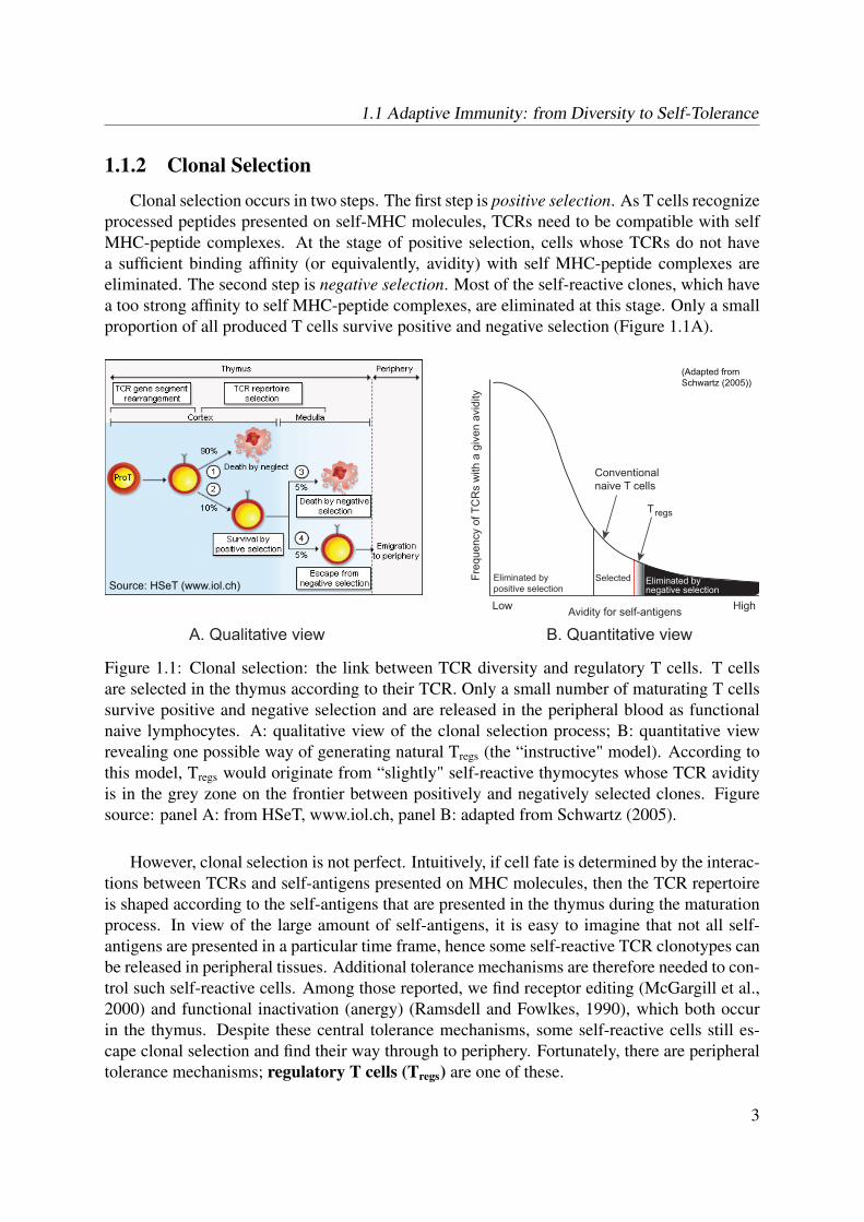
Clonal selection occurs in two steps. The first step is positive selection. As T cells recognizeprocessed peptides presented on self-MHC molecules, TCRs need to be compatible with selfMHC-peptide complexes. At the stage of positive selection, cells whose TCRs do not havea sufficient binding affinity (or equivalently, avidity) with self MHC-peptide complexes areeliminated. The second step is negative selection. Most of the self-reactive clones, which havea too strong affinity to self MHC-peptide complexes, are eliminated at this stage. Only a smallproportion of all produced T cells survive positive and negative selection (Figure 1.1A).
Eliminated bypositive selection
Tregs
Low High
Freq
uenc
y of
TC
Rs
with
a g
iven
avi
dity
Conventionalnaive T cells
Avidity for self-antigens
Source: HSeT (www.iol.ch)
A. Qualitative view B. Quantitative view
(Adapted from Schwartz (2005))
Eliminated bynegative selection
Selected
Figure 1.1: Clonal selection: the link between TCR diversity and regulatory T cells. T cellsare selected in the thymus according to their TCR. Only a small number of maturating T cellssurvive positive and negative selection and are released in the peripheral blood as functionalnaive lymphocytes. A: qualitative view of the clonal selection process; B: quantitative viewrevealing one possible way of generating natural Tregs (the “instructive" model). According tothis model, Tregs would originate from “slightly" self-reactive thymocytes whose TCR avidityis in the grey zone on the frontier between positively and negatively selected clones. Figuresource: panel A: from HSeT, www.iol.ch, panel B: adapted from Schwartz (2005).
However, clonal selection is not perfect. Intuitively, if cell fate is determined by the interac-tions between TCRs and self-antigens presented on MHC molecules, then the TCR repertoireis shaped according to the self-antigens that are presented in the thymus during the maturationprocess. In view of the large amount of self-antigens, it is easy to imagine that not all self-antigens are presented in a particular time frame, hence some self-reactive TCR clonotypes canbe released in peripheral tissues. Additional tolerance mechanisms are therefore needed to con-trol such self-reactive cells. Among those reported, we find receptor editing (McGargill et al.,2000) and functional inactivation (anergy) (Ramsdell and Fowlkes, 1990), which both occurin the thymus. Despite these central tolerance mechanisms, some self-reactive cells still es-cape clonal selection and find their way through to periphery. Fortunately, there are peripheraltolerance mechanisms; regulatory T cells (Tregs) are one of these.
3

CHAPTER 1 : General Introduction
1.1.3 Regulatory T cells
Regulatory T cells (Tregs) are a subset of CD4+ helper T cells. These specialized "con-trollers" act as antagonists to immune responses by suppressing the activation and proliferationof CD4+ helper and CD8+ killer T cells. By this means, Tregs are involved in self-tolerance (Kimet al., 2007), homeostasis and in the control of excessive immune reactions. Several types ofcells exhibit regulatory functions, for example the induced Tregs, the IL-10 secreting TR1 cells,the TGFβ-secreting TH3 cells, or the adaptive Tregs. Here, we focus mainly on the so-callednaturally occurring Tregs.
Naturally occurring Tregs are identified by the surface expression of CD4, as well as bythe expression of the transcription factor forkhead box P3 (FoxP3), a negative modulator ofIL-2 transcription (Fontenot et al., 2003; Hori et al., 2003). These cells are generated in thethymus through mechanisms that are not yet fully understood. Their development is programedand controlled by the master regulator FoxP3 and requires high-affinity interactions betweentheir TCR and self MHC-peptide complexes (Picca et al., 2006). Similarly to the commitmentto CD4+/CD8+ cell lineages, or the differentiation pathways of effector/memory cells, twomodels of thymic Tregs generation have been proposed: a deterministic “instructive" model(Jordan et al., 2001; Lio and Hsieh, 2008; Modigliani et al., 1996) and a “stochastic" selectionmodel (van Santen et al., 2004). In the first, immature thymocytes that are potentially self-reactive commit to the regulatory lineage. The concept can be visualized by considering thedistribution of TCR avidities, result of the TCR gene segment rearrangements (Figure 1.1B).The low avidity cells are eliminated by positive selection, whereas the high avidity cells aredeleted by negative selection. The selected naive (non-regulatory) T cells have TCR avidity thatis neither too high, nor too low. According to the instructive selection model, Tregs would haveTCR avidity in the high end of the avidity spectrum because they originate from potentially self-reactive clones (Schwartz, 2003). In the stochastic selection model, the Tregs lineage conversionsignal would be rather stochastic, independent of TCR avidity.
Tregs ontogeny therefore suggests that these cells are either created as a separate lineagethrough unknown factors independent of TCR specificity (stochastic selection), or they origi-nate from a thymocyte ancestor common to conventional CD4+ T cells, where TCR specificityplays a key role (instructive selection). These two distinct pathways affect the way Tregs areviewed in terms of proliferation capacity. Indeed, the paradigm of central tolerance in the thy-mus states that self-reactive clones are either deleted (Burnet, 1959), or rendered functionallyinactive (anergic) (Ramsdell and Fowlkes, 1990). If the instructive selection model is accepted,it would be logical to think that Tregs are anergic cells, thus have a limited proliferation capac-ity. If, instead, the stochastic selection model is accepted, there is no reason to think that Tregs
would have an impaired proliferation capacity. The dichotomous nature of their ontogeny isprobably at the source of what we call the Tregs “proliferation controversy".
A major challenge in current studies of regulatory T cells is the lack of cell surface mark-ers proper to this population. The expression of the transcription factor FoxP3, which identi-fies Tregs, is intracellular and consequently necessitates the destruction of cells for detection.Moreover, FoxP3 does not solely identify thymus-derived Tregs, but also cells that have ac-quired suppressive phenotype and functions in the periphery (Curotto de Lafaille et al., 2004;
4

1.2 Mathematical Modeling in Immunology
Vukmanovic-Stejic et al., 2006) 1. The cell surface marker mostly used hitherto is CD25, theα-chain of the IL-2 receptor, which has been shown to be constitutively expressed on Tregs
(Baecher-Allan et al., 2001; Miyara et al., 2009b; Sakaguchi et al., 1995; Taams et al., 2002).However, CD25 is also expressed transiently on activated (non-regulatory) T cells, which ren-ders the isolation of Tregs difficult. Several other markers have been associated with naturallyoccurring Tregs, notably high levels of CTLA-4 (cytotoxic T-lymphocyte associated molecule-4), CD62L, CCR7, GITR (glucocorticoid-induced TNF receptor) and low levels of CD127 (thealpha-chain of the IL-7 receptor) (Codarri et al., 2007; Liu et al., 2006; Seddiki et al., 2006a).Currently, the combination of high or low expression levels of several of the above surfaceproteins are used to detect Tregs within a reasonable degree of purity (reviewed in Sakaguchiet al. (2010)). Hitherto, a typical experimental approach consists in isolating CD4+CD25+ Tcells, performing the desired experiment, and verifying a posteriori the enrichment of Tregs inthe sample by immobilizing the cells.
Robust Treg cell identification is one among many unresolved issues related to these cells.Although important advances have been recently made, the main molecular mechanism(s) ofTregs-mediated suppression in humans remain elusive. It is established that Tregs need to beactivated through their TCR to be functionally suppressive and the strength of TCR stimulationinfluences the effectiveness of suppression. Moreover, suppression can be contact-dependentor cytokine-mediated (see Sakaguchi et al. (2010) for a review). Despite the remaining openquestions, the broad range of clinical applications of regulatory T cells (Miyara et al., 2009a;Safinia et al., 2010; Trzonkowski et al., 2009) is rendering this research area very active andintriguing.
1.2 Mathematical Modeling in Immunology
With the modern advances of experimental techniques, a large amount of immunologicaldata is created. The complexity of interactions between individual components and the dif-ficulty to isolate influencing factors makes the use of mathematics challenging, but valuable.Mathematical models in immunology exist since several decades. Like any other research fieldwhere two or more disciplines are crossing, the challenges of modeling a biological phenom-ena are multiple. The size of a living system, the number and the complexity of interactionsbetween individual components is such that tractable and computationally efficient models aredifficult to derive. Nevertheless, mathematical models have been applied to immunology sincemore than 50 years (Louzoun, 2007).
In this thesis, we develop mathematical models in order to gain biological insight and im-prove the interpretation of T-cell-related experimental data. The dissertation is divided in twoparts, each part addressing the following immunological questions: (I) the in vivo dynamicsof human regulatory T cells; (II) the measurement of the structural diversity of a TCR samplewith the AmpliCot technique.
1. Moreover, a non-regulatory FoxP3-expressing CD4+ T cell population has been recently discovered in theperipheral blood of humans (Miyara et al., 2009b).
5

CHAPTER 1 : General Introduction
1.3 Dissertation Outline
The dissertation is structured as follows. In Chapter 2, we define a generic model thatdescribes the lifelong dynamics of regulatory T cells. We use our model to address the Tregs
proliferation controversy. In that perspective, we derive from the generic model several bio-logically plausible scenarios about the origins and the proliferation capacity of these cells. Themodel scenarios are challenged against human ex vivo data and some of them are discarded.
In Chapter 4, we address the general question of TCR diversity by improving the interpreta-tion of AmpliCot, an experimental technique that aims at the diversity measurement of nucleicacid sequences. We use mathematical modeling to describe AmpliCot experimental data. Onceagain, we evaluate two model variants by fitting them to data. Practical and methodologicalconclusions are then drawn.
Chapter 3 and Chapter 5 are auxiliary chapters that contain theoretical and analytical resultsrelated to the Tregs and the AmpliCot models respectively. We make concluding remarks inChapter 6.
6
Part I
Dynamics of Regulatory T cells


Chapter 2Lifelong Dynamics of Human CD4+CD25+Regulatory T Cells
2.1 Introduction
As of today, two developmental pathways of human regulatory T cells in vivo have beenidentified (Sakaguchi, 2003): naturally occurring thymus-derived Tregs (Fritzsching et al., 2006;Hoffmann et al., 2006; Seddiki et al., 2006b; Wing et al., 2002) and adaptive or induced Tregs,derived from non-regulatory CD4+CD25−FoxP3− T cells (Kretschmer et al., 2005; Vukmanovic-Stejic et al., 2006; Walker et al., 2003a). Naturally occurring Tregs originate in the thymus andare released in the periphery with a naive phenotype (Cupedo et al., 2005; Seddiki et al., 2006b;Takahata et al., 2004; Wing et al., 2002, 2003). They are identified as CD4+CD25+CD45RO− Tcells and will be called “precursor" Tregs throughout this chapter 1. Once precursors encountertheir cognate antigen, they acquire a suppressive capacity and a memory phenotype (Fritzschinget al., 2006). We call these differentiated cells “mature" Tregs. Adaptive Tregs are derived fromrapidly proliferating activated-effector or memory CD4+CD25− T cells that acquire the per-manent expression of CD25 and the suppressive function in the periphery (Vukmanovic-Stejicet al., 2006; Walker et al., 2003a). Because they have experienced antigen, these cells havea mature profile and express the memory phenotype CD45RO. It is important to remark thatthere is no difference regarding the surface markers characterizing both types of mature Tregs
and consequently, one can not distinguish both Tregs origins using fluorescent techniques. Thesame observation can be made about T-cell receptor excision circles (TREC): Tregs from bothorigins have similar decreased TREC content (Kasow et al., 2004). Thymus-derived regulatorycells divide during clonal selection in the thymus and in the periphery, whereas activation-induced regulatory cells come from rapidly proliferating non-regulatory T cells and thereforehave decreased TREC content.
In vivo studies of human Tregs have shown that the number of precursors decreases signifi-cantly with age (Seddiki et al., 2006b; Valmori et al., 2005), whereas the number of mature Tregs
increases in elderly individuals (Gregg et al., 2005). Thymic involution, together with the fact
1. These cells are also named naive Tregs (Miyara et al., 2009b).
9

CHAPTER 2 : Lifelong Dynamics of Human CD4+CD25+ Regulatory T Cells
that CD4+CD25+CD45RO+ mature regulatory T cells are known to be non-proliferating, intro-duces the question of how is developed and maintained a stable pool of Tregs throughout life.Different hypotheses are evoked in Akbar’s opinion paper (Akbar et al., 2007); the question ofproliferation is central. The first hypothesis claims that precursor CD4+CD25+CD45RO− cellsare able to proliferate (Klein et al., 2003; Walker et al., 2003b) and even though the thymicinvolution reduces the input of newly produced precursors with age, these cells are the mainreservoir of mature Tregs. The second hypothesis suggests that both precursor and mature Tregs
are non-proliferating but although mature Tregs are sensitive to death because of their high levelsof CD95 (Fritzsching et al., 2006; Taams et al., 2001), the fact that precursors are apoptosis-resistant suffices to sustain a stable pool of mature Tregs. Finally, the third hypothesis points outthe presence of an external source of mature Tregs, derived from rapidly proliferating effectorCD4+CD25− T cells (Taams et al., 2001; Vukmanovic-Stejic et al., 2006). Thus, there is acontroversy about the mechanisms by which Tregs regenerate throughout the lifetime of indi-viduals. The objective of our study is to evaluate the above biological hypotheses by the meansof a mathematical model and to measure their effect on the development and maintenance of apool of human Tregs.
A major difficulty encountered in mathematical modeling of biological systems is dealingwith parameter values. The more detailed the model is, the more parameters it involves and itsbehavior can be completely different according to the values taken by the latter. Good parame-ter estimates exist in some cases, but it is often difficult to build an experiment that allows fortheir direct measurement. In the mathematical model presented hereafter, we employ a mod-eling technique that alleviates the parameter estimation problem by considering parameters asrandom variables having a priori distributions (as in Bayesian approaches). This approachallows us to evaluate simultaneously several values, to produce results that depend little onthe exact values, and therefore to diminish the probability of errors due to wrong parameterestimates.
Using the above technique, we define a generic model describing the lifelong dynamicsof Tregs. We attempt to include in it all the actual knowledge about the population dynamicsof regulatory T cells, while keeping the model as simple as possible. We consider all eventsthat affect the population size of Tregs: immune reactions to self or foreign antigens, the home-ostatic activity and the external input – from the thymus or from the non-regulatory effectorCD4+CD25− T cell pool. We then implement the above-mentioned hypotheses about the ori-gins and proliferation capacity of Tregs. In order to validate the model, we compare it to humandata consisting in measurements of Tregs as a function of age. We first study the expectedmodel behavior where the stochastic parameters take the average value of their a priori distri-butions. Then, we evaluate the performance of the model with random parameters. Its behavioris evaluated for several values inside the given parameter range and the density of trajectoriesis estimated. This density leads to the definition of the likelihood of a model scenario, used toformally reject the scenarios that are unable to fit the data.
2.1.1 Mathematical Models of Tregs: State of the Art
As of today, a certain amount of mathematical models of regulatory T cells can be foundin the literature. Most of them analyze the suppression mechanisms of these cells and their
10

2.1 Introduction
interactions with other cell types and cytokines. In this section we give an overview of the cur-rently existing work. For each cited study, in addition to the main findings, the methodologicalapproach is highlighted. We also mention whether Tregs were considered as proliferative or not.
Crossregulation Model of Immunity (Tregs and APCs)
The most extensively studied and developed model of regulatory T cells is certainly theCrossregulation model of immunity (León et al., 2000). In their original paper, León et al.(2000) test several suppression mechanisms by considering populations of antigen presentingcells (APCs), regulatory and conventional T cells. The authors postulate that the cell-mediatedsuppression occurs through the formation of multicellular conjugates of T cells and APCs.Three suppression scenarios are examined: (1) competition between Tregs and conventional Tcells for conjugation sites on APCs; (2) proliferation inhibition of conventional T celly by Tregs
on conjugates with APCs; (3) in addition to the proliferation inhibition, the growth of Tregs
is hypothesized to be dependent on conventional T cells. The model is described by ordi-nary differential equations (ODE) and a quasi-steady state assumption is applied to conjugates(which significantly simplifies the equations). The authors identify different parameter regimes,according to which the equilibrium points might change (and bi-stability appears). Using aphase-plane and bifurcation analysis, each possible scenario is related to existing experimentalobservations (qualitatively). To account for the outcome of adoptive transfer experiments, theauthors conclude that the correct suppression model should exhibit bi-stability, leading to atolerant and an auto-immune steady state, where either Tregs or effectors dominate. The thirdsuppression model is retained as most plausible: active growth suppression of effectors by Tregs
and maintenance of Tregs dependent on effectors (through IL-2).The same model is then applied to the analysis of experimental data of linked suppression
in vitro (León et al., 2001). The experimental set up consists in APCs and target conventionalT cells that are co-cultured with or without Tregs. Target cells are stimulated and the populationexpansion is measured. It is hypothesized that when conjugated with Tregs simultaneously, theproliferation of conventional T cells is reduced. The inhibition index is defined as the ratiobetween the cell counts in a culture containing Tregs and those in a culture without Tregs. In thismodel, Tregs are assumed to be non-proliferative and two mechanisms of suppression are ex-amined: simple competition for APC conjugation sites versus competition + active inhibition.The authors observe that the inhibition index is mainly determined by the number of regulatorycells per APC and is insensitive to the number of target (suppressed) cells. However, they failto fit the model to the experimental data and put forward several explanations, among whichthe possibility that Tregs proliferate in the presence of IL-2-producing conventional T cells.
In the subsequent study, León et al. (2003) further develop the Crossregulation model toadd thymic input and the simultaneous peripheral dynamics of several T cells clones. This isdone by simulating clonal selection. New clones are generated stochastically and the equationsdescribing their dynamics are appended to the existing ODE system. If the population size of aparticular clone vanishes, its corresponding equation is removed. The system is then perturbedin order to simulate two types of events: the introduction of a foreign antigen and its clearance.After each external perturbation, the new steady state is computed. This is different than oursystem, where immune reactions are internally generated by the stochastic process. The authors
11

CHAPTER 2 : Lifelong Dynamics of Human CD4+CD25+ Regulatory T Cells
test the effect of thymectomy and observe that diversity is lost by competitive exclusion.
The Crossregulation model is used by León et al. (2004) to study the correlation betweenthe incidences of autoimmune diseases and infection. An inverse correlation is revealed: therisk of autoimmunity is the price that must be paid for assuring immune responses to pathogens.
Carneiro et al. (2005) further study an alternative self-tolerance mechanism, mediated bythe tuning of activation thresholds, which would make auto-reactive T cells reversibly "anergic"and unable to proliferate. It turns out that this hypothesis is only partially compatible with thequalitative observation of adoptive transfer experiments and was therefore left out.
The Crossregulation model was also applied to study tumor immunobiology. León et al.(2007a) provide an explanation to the observation that the development of some tumors expandregulatory T cells, whereas others do not. In a subsequent study (León et al., 2007b), thesame authors consider how these two tumor classes respond to different therapies, namelyvaccination, immune suppression, surgery, and their different combinations. Model responsesto different therapies are simulated as particular dynamical perturbations to the ODE system.
In a review paper, Carneiro et al. (2007) gather all the above facts and observations revealedby the Crossregulation model, both theoretical and experimental, in an unifying theory in which"the persistence and expansion of Tregs depend strictly on specific interactions they make withAPCs and conventional effector T cells." Although the importance of APCs in the function ofTregs is largely emphasized in the Crossregulation model, throughout all the papers, the actualdynamics of these cells are either considered as a parameter or as an externally controlledvariable. The following work brings more attention to the explicit dynamics of APCs.
Tregs and APCs
Alexander and Wahl (2010) model antigen-specific natural Tregs, together with a particulartype of self-antigen, its corresponding APCs and the responding effectors. The authors focuson a positive feedback loop between effectors that release antigens, which are taken up byAPCs that, in turn, stimulate more effector T cells. The production of Tregs is proportionalto both effectors (IL-2 producing cells) and APCs and they act by suppressing the action ofAPCs. Different suppression mechanisms are analyzed. Interestingly, the authors present both adeterministic and a stochastic version of the same system. The ODE system reveals bi-stability,as in most Tregs models, with a trivial (tolerance) and non-trivial (auto-immune) stable state.The limit behavior determined by the basic reproductive ratio R0. The stochastic version of theODEs is derived using an approach similar to the one of Chao et al. (2004), in which the ODEsare discretized and the populations are updated at each time step by generating Binomial orPoisson random variables. Once again, the model is not challenged against experimental data.One of the conclusions is that self-antigen-specific Tregs play no role in the system’s qualitativelong-term behavior, but have quantitative effects that could potentially reduce and clear an auto-immune response. The important role of Tregs with arbitrary specificity is highlighted. Finally,the probability of developing a chronic auto-immune disease increases with the quantity ofinitial-exposure antigen or of auto-reactive effectors.
12

2.1 Introduction
Tregs and Cytokine Kinetics
Burroughs et al. (2006) study regulatory and auto-immune (conventional) T cells by assum-ing that all cell interactions are realized through cytokines. In particular, the authors observethe consequences of Tregs inhibition of IL-2 secretion. Their model is composed of restingand activated regulatory and auto-immune T cells, as well as two cytokines: IL-2 producedby auto-immune cells and consumed by both auto-immune and regulatory T cells, and anothercytokine, produced by tissues, consumed by Tregs only. Tregs inhibit the secretion of IL-2 and donot produce IL-2 themselves. It is assumed that Tregs proliferate homeostatically by competingfor the tissue-secreted cytokine. In addition, these cells can also proliferate in the presenceof IL-2, but less efficiently than conventional T cells. The stability analysis of the ODE sys-tem reveals a "control" state in which Tregs dominate and eliminate auto-immune cells, and an"auto-immune" state in which the latter expand and escape Tregs control. The main conclusionof this theoretical work is that the shift towards control or auto-immunity is dependent on theefficiency of auto-immune T cells to utilize IL-2 compared to Tregs. This efficiency can be com-pensated by auto-immune cells by an increase in their number. In a later paper, Burroughs et al.(2008) further analyze the above model and provide a sensitivity analysis to the parameters.
More recenlty, Garcia-Martinez and León (2010) extend the Crossregulation model by ex-plicitly modeling the dynamics of IL-2. By doing so, they allow for non-local/unspecific in-teractions between effectors and Tregs in the sense that interactions are possible not only uponsimultaneous conjugation on the same APC, but also via the free IL-2 present in the samelymph node. Thus, this model combines the assumptions of the Crossregulation model and themodel of Burroughs et al. (2006) and constitutes a rather complete picture of the cell interac-tions in a lymph node. The same methodological approach as in León et al. (2000) is applied.Two model variants, with different roles of IL-2 in suppression, are tested: (1) Tregs suppresseffectors by competition for IL-2 only; (2) in addition to competition, Tregs inhibit the activa-tion of effectors co-localized on the same APC. The authors establish parameter constraints inthe extended models in order to reproduce the basic properties of the Crossregulation model(bi-stability, etc.). Furthermore, the extended models lead to new properties of the dynamics.An interesting characteristic regarding the unspecific regulation is observed. The authors con-sider the case of two different antigen-specific clones of effectors and Tregs responding to twosets of APCs. An abrupt increase in the number of APCs of type 1 is then applied, simulating,for example, a particular infection. In version (1) of the model, the responses to both types ofAPCs are fully coupled. This means that the increase in APCs of type 1 can break tolerancefor the corresponding cells (effectors of type 1 take over Tregs of type 1) and the same wouldhappen for the cells of type 2. This would lead to collateral damages if all clones are activatedby the stimulation of a single one. The situation is more realistic in model variant (2), wherethe activation of clone of type 1 does not imply the activation of the other clone.
Adaptive/Induced Tregs
Fouchet and Regoes (2008) model an interaction network composed of adaptive Tregs, effec-tor T cells and APCs. The model is very similar to one version of the Crossregulation model,except for the fact that resting APCs can induce the transformation of effectors into Tregs. Theauthors define an ODE system in which precursor T cells may differentiate into either adaptive
13

CHAPTER 2 : Lifelong Dynamics of Human CD4+CD25+ Regulatory T Cells
Tregs or effector T cells, depending on the activation state of the APC. An equilibrium analy-sis reveals the existence of two stable equilibriums (similarly to the Crossregulation model):one tolerant (regulated) state where Tregs control effectors and one unregulated state where thevanishing population of Tregs cannot control the effectors. Then the authors study the effectof parameters on the nature of the equilibrium regime. The bifurcation analysis reveals thatthe switch from the regulated to the unregulated state depends on the strength of the antigenicstimulus and the state from which the network has been perturbed.
In their experimental study of adaptive Tregs, Vukmanovic-Stejic et al. (2006) use the modeldeveloped in Macallan et al. (2003) to estimate the in vivo proliferation and death rates ofmemory-derived FoxP3+ regulatory T cells. The latter model is specifically defined for la-beling experiments, where deuterium from deuterated glucose is incorporated into the DNAof dividing cells. The model has one compartment, the amount of labeled deoxyadenosine,and accounts for its appearance and disappearance due to cell proliferation and death (furtherdeuterium labeling models can be found in Mugwagwa (2010)). The analysis of experimen-tal data reveals the peripheral conversion or rapidly proliferating CD4+CD25−FoxP3− memoryeffectors into a regulatory CD4+CD25hiFoxP3+ phenotype.
After developing an extremely detailed delay differential equations (DDE) model to studythe role of natural Tregs in the adaptive immune system (Kim et al., 2007), Kim et al. (2010)study the dynamics of primary T-cell responses and the possible involvement of adaptive regu-latory T cells. The authors challenge the paradigm of a primary T cell response, according towhich, (1) T-cell dynamics in response to an antigen do not depend on the level and durationof antigen stimulation; and (2) T-cell responses are independent of the clone size of antigen-specific responders. Using delay and partial differential equations, the authors conclude thatthe old "paradigm does not entirely capture the observed robustness of T cell responses to vari-ations in precursor frequency". They propose an alternative mechanism in which the dynamicsof a primary T-cell response are governed by a feedback loop involving adaptive regulatorycells rather than by intrinsic developmental programs.
Tregs and Gene Expression
In a general setting of helper T cell differentiation, Van den Ham and de Boer (2008) pro-pose a model describing the expression of master regulators. Master regulators are transcriptionfactors that are both necessary and sufficient for the induction of a certain cellular phenotype.For example, to polarize a helper T cell towards the helper 1 type, Tbet is necessary, whereasfor helper type 2, it is GATA3. In the case of Tregs, FoxP3 is the master regulator. The gen-eral framework of Van den Ham and de Boer (2008) has been applied to experimental datameasuring the expression levels of FoxP3 and GATA3 mRNA.
Tregs and Evolution
Saeki and Iwasa (2009) develop a mathematical model to study the advantages of havingregulatory T cells in the immune system. The authors weight the pros and the cons of a robustability to cope with foreign antigens, versus auto-immunity. Using a probabilistic approach,they define the fitness function of an organism, which takes into account the benefit of having
14

2.1 Introduction
effector T cells reactive to foreign antigens and the severity of having effectors attacking selftissues. A model of cell maturation in the thymus is presented, where immature T cells aredetermined to be regulatory or effectors, based on whether or not they interact with self-antigensduring clonal selection (they also consider another version, where cell fate is pre-determined).It is assumed that the number of times a particular auto-reactive immature T cell meets withits corresponding antigen during clonal selection follows a Poisson distribution. Further, oncein the periphery, activated Tregs are assumed to suppress effectors by direct interaction. ThePoisson distribution is again used to model the number of times a particular effector T cellmeets regulatory T cells. From this is calculated the probability of a cell not being suppressed.The fitness function of a system with Tregs is then compared to the fitness without Tregs andconclusions are drawn with respect to the parameters. Localized and global suppression arecompared. It turns out that it is advantageous to have regulatory T cells if suppression islocalized, i.e., "if the body is composed of many compartments, and regulatory T cells suppressthe immune reactions only within the same compartment". The framework presented by theauthors gives an interesting insight of T cell maturation and Tregs formation.
In the following paper, Saeki and Iwasa (2010) use an extension of the same mathematicalmodel to study the optimal number of regulatory T cells. The authors propose that this num-ber depends on the "number of self-antigens, the severity of auto-immunity, the abundance ofpathogenic foreign antigens, and the spatial distribution of self-antigens in the body."
2.1.2 Our Contributions
None of the above models has studied in depth the quantitative effect of Tregs proliferationcapacity and origins on the lifelong peripheral pool size in humans. At the time of developmentof our model, the proliferation capacity of Tregs was a controversial issue. Our first contributionis therefore to address quantitatively this question and to challenge the plausibility of severalhypotheses with human ex vivo data.
From the perspective of proliferation capacity of Tregs, the model of Burroughs et al. (2006)is the closest one to ours, because it considers strict conditions for Tregs proliferation. However,the authors of this study did not consider the lifelong dynamics resulting from the repeatedexposure to self- or foreign- antigens.
None of the above studies has sorted Tregs on the expression of the memory-type receptorCD45RO. Once again, the closest discrimination was in Burroughs et al. (2006), where theauthors consider active and inactive Tregs, which was mainly translated in a suppression capacitydifference. In addition to distinguishing the activated from the resting Tregs populations, wealso account for antigen-unexperienced precursors, which were known to have only a limitedsuppression and a marked proliferation capacity.
A striking difference between our model and most of those studying Tregs dynamics is thefact that we neglect the population of APCs. However, only in Alexander and Wahl (2010)are the dynamics of APCs modeled explicitly. In all the variants of the Crossregulation model(Carneiro et al., 2007), the APCs are assumed to be in equilibrium and their presence is onlyexpressed through one parameter, the density of APC conjugation cites. Thus, these modelsreduce to a predator-pray system, where either one of the conventional or regulatory T cellsoutcompetes the other, either both populations co-exist. Our intention is to start by building
15
CHAPTER 2 : Lifelong Dynamics of Human CD4+CD25+ Regulatory T Cells
the simplest possible model that can address the relevant question. As we are not concernedwith suppression mechanisms, we ignore APCs and conventional T cells. The effect of IL-2as a growth factor is modeled implicitly through the parameters. Nevertheless, the inclusion ofthese components would certainly be of interest.
Our second contribution is the fact that our model is conceptually different from the existingTregs models. Indeed, the combination of a stochastic process with ODEs is an original approachthat has not been applied to the study of T cell dynamics. In addition, we employed randomparameters with a Bayesian-type statistical analysis, which is also a marginal manner of treatingunknown parameter values.
Finally, we have fitted a quantitative model to time-series experimental data, which has notyet been done in the case of human regulatory T cells. Hitherto, data sets have been used tofit the time-dependent dynamics of conventional CD4+ or CD8+ T cells (De Boer et al., 2003;Mugwagwa, 2010).
2.1.3 Chapter Outline
This chapter is organized as follows. We first present in Section 2.2.1 the detailed de-scription of the model, followed by the materials and methods necessary to the data obtention(Section 2.2.2). In Section 2.2.3, we describe how the model is fitted to the data and howthe scenarios are formally evaluated. The results are in Section 4.3 and the discussion in Sec-tion 4.4.
16

2.2 Materials and Methods
2.2 Materials and Methods
2.2.1 Tregs Mathematical model
In order to model the biological hypotheses concerning the origins and the proliferationcapacity of Tregs, we consider several scenarios of a generic mathematical model. The scenariosare the result of imposing constraints on model parameters such as the input, proliferation anddeath rates of precursor and mature Tregs in the generic model.
We use several mathematical tools in order to describe in a robust way Tregs lifelong ki-netics. Changes in the populations’ sizes due to immune reactions and homeostatic activityare described by ordinary differential equations (ODEs). Events corresponding to encounterswith antigen-presenting cells leading to (auto-)immune responses are generated according to astochastic process. A sketch of the entire system with all its components can be seen in Fig-ure 2.1. For a quick reference, Table 2.1 summarizes all the assumptions of our model. In whatfollows, we describe in detail the generic model, the model scenarios, the parameter fitting andthe model evaluation procedure.
Generic model
The generic model describes the lifelong dynamics of Tregs. We call it generic because itis taking into account all possible events that may affect Tregs population size and because it isa generalization out of which we define the model scenarios that describe the studied biolog-ical hypotheses. The generic model is composed of two parts: a deterministic part describingcell dynamics during immune responses and homeostasis, and a stochastic part generating allinfection events occurring in a human lifetime.
(Auto-)Immune reactions process In order to study the dynamics of regulatory T cells overthe entire lifetime of a human, responses to self- and foreign-antigens are included in our model.We consider two types of immune reactions: the minor ones, occurring frequently and triggeredby self- or dietary antigens, and the major ones, occurring rather seldom, mainly provoked byforeign antigens and having a great impact on the Tregs pool. Minor immune reactions trig-gered by antigens sampled in the mucosa-associated lymphoid tissues are taken into accountin the pool-size control dynamics described in the next section. Major immune reactions aretriggered by successful interactions with antigen-presenting cells, in which a cytokine environ-ment allowing Tregs activation and (possibly) proliferation is present (Carneiro et al., 2007). Aswe found no information about the frequencies and time-distribution of such immune reactionsin vivo, we model this phenomena with a stochastic process having a constant rate. Thus, weassume the length of time-intervals between two infections to be random, having a shifted ex-ponential distribution with mean λ+δ, where δ is the minimal duration of an immune response.We make the simplifying assumption that during the first phase of an immune response (oflength δ), no other infections are occurring and that the capacity to present self-peptides is notaltered with time in healthy individuals. We call {τn}n∈N the stochastic process of infectiontimes. The dynamics of cells between the events of the stochastic process are described in whatfollows.
17

CHAPTER 2 : Lifelong Dynamics of Human CD4+CD25+ Regulatory T Cells
Figure 2.1: A sketch of the different components of the mathematical model. A: The outputof our mathematical model are cell counts as function of time. We are considering three celltypes, namely CD4+CD25+CD45RO− precursor Tregs and CD4+CD25+CD45RO+ quiescent oractivated mature Tregs. B: The model is composed of a stochastic process generating the eventscorresponding to successful encounters with antigen-presenting cells leading to (auto-)immuneresponses. These responses are characterized by a transient increase in the activated matureTregs population. C: The dynamics of cells between two events of the stochastic process are de-scribed using ordinary differential equations. These equations take into account all events thataffect the cell population size. A detailed description of each component of the cell dynamicscan be found in the Generic Model section.
Cell dynamics Based on the expression of the surface protein CD45RO, one can sort twosubpopulations of Tregs: CD4+CD25+FoxP3+CD62L+CD45RO− precursor and CD4+CD25+-FoxP3+CD62L+CD45RO+ mature Tregs. For the sake of the mathematical model, we considera third population that we call activated mature Tregs and that has the same surface receptorsas the quiescent mature Tregs
2. Activated mature Tregs are composed of both precursors thatexperience peripheral antigens for the first time (they can be also activated precursors thathave just acquired the mature phenotype), and mature Tregs that are recruited into a secondaryimmune response. Thus, the mathematical model has three compartments: P , the precursorTregs, Q, the quiescent mature Tregs, and R, the activated mature Tregs.
2. Note that the population of activated Tregs has been recently discovered as part of the peripheral in vivo poolof human Tregs (Miyara et al., 2009b). We position our model with respect to this new perspective in Chapter 6.
18

2.2 Materials and Methods
a) Immune responses. In vitro experiments show that following acute antigenic stimula-tion, precursor Tregs activate and up-regulate the memory-type CD45RO receptor, as they loosetheir naive phenotype CD45RA receptor (Fritzsching et al., 2006; Valmori et al., 2005). In themeanwhile, they differentiate into mature Tregs able to exert their suppressive function. Oncethe antigenic stimulation is lost, a small proportion of all activated Tregs becomes long-livedmature cells, and the others die by apoptosis, similarly to other lymphocytes. As we are notmodeling the dynamics of other cell types and of pathogens, we apply the two-phase immuneresponse model used to describe CD4+CD25− and CD8+ cell dynamics (Althaus et al., 2007;De Boer et al., 2003, 2001; Fouchet and Regoes, 2008). We call τn the beginning of the nth
immune response to a foreign antigen (n ∈ N) and τn + δ the time at which the expansion phaseends. We assume that the effect of antigen on cells has a fixed duration δ, after which cells
Biologicalprocess
Assumptions
(Auto-)Im-munereac-tionsprocess
1. Major immune reactions modeled as a stochastic process with one(constant) parameter.
2. Minor immune reactions triggered by antigens sampled in themucosa-associated lymphoid tissues included in the homeostasisactivity.
3. Capacity to present self-peptides is not altered with age in healthyindividuals.
4. During the fixed phase of an immune reaction, no other reactionsare allowed.
Immuneresponses
5. Two-phase immune response: a first phase of fixed length and asecond phase of random length.
6. Exponential expansion/contraction of cells following immunogenstimulation.
7. 10% of the expanded population of activated Tregs becomes long-lived mature Tregs.
Homeostaticactivity
8. Unique source of precursors: thymus.9. Four possible sources of mature Tregs: thymus, differentiation of
precursors, phenotype switching of effector CD4+CD25− T cells,and homeostatic proliferation.
10. Time-dependent thymic involution (exponential decline).11. Constant rate of generation of Tregs from rapidly proliferating
CD4+CD25− effector T cells under certain conditions.
Antigenspecificity
12. The size of the responding clone is chosen randomly (uniformdistribution).
Primary /secondaryinfections
13. The probability of primary infections is declining with age andis such that children experience a majority of primary infectionsand adults, a majority of secondary infections.
Table 2.1: Summary of all model assumptions.
19

CHAPTER 2 : Lifelong Dynamics of Human CD4+CD25+ Regulatory T Cells
stop their intense proliferation phase (Phase 1) and start dying by activation-induced cell death(Phase 2).
During Phase 1, precursor Tregs may divide, die, or convert into mature effector cells atrate b. Quiescent mature Tregs activate at rate f cells per day. Effector mature Tregs may alsoproliferate and die. As the first phase is an expansion phase, we only consider a net populationexpansion rate, which should be interpreted as the cumulative effect of proliferation and deathin the population of precursors (resp. activated mature Tregs). Thus, for parameter identificationissues, we consider only one rate, called aP > 0 (resp. aR > 0), which is the net populationexpansion rate. The following differential equations express the dynamics of the expansionphase:
P = (aP − b)PQ = −fQ (2.1)R = bP + fQ + aRR
During Phase 2, precursor Tregs die at rate dP per day. Activated mature Tregs die at ratedR and convert to long-lived mature cells at rate c per day. The long-lived mature quiescentTregs have a slight decrease in their population size expressed by death rate dQ. The differentialequations corresponding to the contraction phase are the following:
P = −dPPQ = −dQQ + cR (2.2)R = −(c + dR)R
b) Homeostatic activity. The biological processes included in the homeostatic activityare the proliferation and death of cells for regulation of the population size, the death of cellsbecause of their limited lifespan and the input of newly produced cells from the thymus offrom another external source. We hypothesize two types of basal proliferation and death: aconstant and density-dependent one. We call d′ the constant death rate accounting for thelimited lifespan of cells. We assume that a slow and steady cell division occurs at rate a′.Nevertheless, these constant renewal and death rates can not account for self-regulation of thecell population size. In a homeostatic situation, cell numbers are regulated by competition forlimited resources, such as cytokines. This regulation can be achieved in three ways: density-dependent proliferation, density-dependent death or both. The exact way in which regulatory Tcells perform their homeostatic regulation is currently unknown. It is however known that thein vivo homeostatic proliferation of murine natural Tregs is not impaired by their anergic state(Gavin et al., 2002) and that this proliferation is involved in a feedback regulatory loop betweendendritic cells and Tregs (Darrasse-Jeze et al., 2009).
Because the homeostatic activity is an important issue to studying the lifelong dynamicsof cells in vivo, we are considering all possible mechanisms that may have an effect on themodel’s outcome. Thus, we assume that homeostasis of precursors is achieved through density-dependent death at rate ϕP . For mature Tregs, we consider both a density-dependent death atrate ϕQ and a density-dependent Michaelis-Menten type proliferation at rate α, appropriate to
20

2.2 Materials and Methods
make up for lymphopenic situations. Recent thymic emigrants enter both precursor and ma-ture Tregs populations at a time-dependent rate g(t) = gP (t) + gQ(t). The constant term sQ,added to the quiescent mature Tregs population, represents the constant generation of regula-tory T cells from rapidly proliferating CD4+CD25− effector T cells under certain conditions(Akbar et al., 2007; Vukmanovic-Stejic et al., 2006). Remark that we only add this term tothe quiescent mature Tregs population, because we assume that the unique source of precursorCD4+CD25+CD45RO− T cells is the thymus. In addition, cells that are derived from rapidlyproliferating CD4+CD25− cells are antigen-experienced and thus have probably acquired thememory phenotype CD45RO before converting to FoxP3+ regulatory cells. The differentialequations describing the homeostatic activity are the following:
P = gP (t) + (a′P − d′P )P −ϕPP2
Q = gQ(t) + sQ��������������������������������������������External
contribution
+(a′Q − d′Q)Q�����������������������������������������������������Density-
independentregulation
+( α
1 +Q/QM
−ϕQQ)������������������������������������������������������������������������������������������������������������������������Density-dependent
regulation
Q (2.3)
R = 0,
where QM is the size of the mature Tregs population for which the homeostatic renewal of cellsis half of the maximal rate α. Let hP = a′P − d′P and hQ = a′Q − d′Q be the cumulative effects ofthe constant renewal/death rates, hP ∈ R and hQ ∈ R. Whenever negative, we will refer to theseparameters as lifespan of precursors and mature Tregs. The thymic involution is represented asa decreasing exponential function of rate ν (Dutilh and De Boer, 2003; Marusic et al., 1998;Steinmann et al., 1985):
gP (t) = σP exp(−νt)gQ(t) = σQ exp(−νt),
where σP = σ0∗%CD25thymus∗pthymus, σQ = σ0∗%CD25thymus∗(1−pthymus),%CD25thymus is thepercentage of CD25+ cells inside thymic CD4+ T cells, pthymus is the percentage of precursorsinside CD25+cells that are output from the thymus, and σ0 is the estimated thymic output ofCD4+ cells in a newborn.
c) Antigen specificity. To ease the notation in what follows, let Y = (P,Q,R)′. Antigenspecificity is implemented in the following way. Eq. (2.1) and Eq. (2.3) are applied to a propor-tion πn of the total number of Tregs, those representing the antigen-specific clone responding tothe antigen that caused the immune reaction at time τn. We call this population Yclone(τn). Theother 1 − πn proportion of cells do not participate in the nth immune reaction and execute theirhomeostatic activity (Eq. (2.3)).
d) Primary/secondary infections. We take into account the difference between primaryand secondary infections: when some antigen is encountered for the first time, no memory cellsexist, but if the exposure is secondary, the organism already has memory cells associated to itat the time of exposure τn. We call q(t) the probability that an infection at time t is primary and
21

CHAPTER 2 : Lifelong Dynamics of Human CD4+CD25+ Regulatory T Cells
0 20 40 60 80 1000
0.1
0.2
0.3
0.4
0.5
0.6
0.7
0.8
0.9
1
Time (years)
q(t)
Median2.5% quantile97.5% quantile
Figure 2.2: The probability q(t) of a pri-mary infection is decreasing with age.An estimation of the distribution for q(t)defined in Eq.(4) with parameters sam-pled from the a priori distributions of Ta-ble 2.4.
does not involve mature Tregs. Thus, with probability q(τn), the responding clone at time τn isset to Yclone(τn) = πn(P (τn),0,0)′. Otherwise, with probability 1−q(τn), the responding cloneis set to Yclone(τn) = πn(P (τn),Q(τn),0)′. Intuitively, the unexperienced immune system ofyoung individuals is confronting more primary infections than adults. We therefore define thefollowing sigmoid function describing phenomenologically the time-dependence of parameterq:
q(t) = K1 −K2
1 + exp(ω(t − th)) +K2 (2.4)
where K1 is the (approximate) proportion of primary infections at birth, K2 is the limit pro-portion of primary infections at adulthood, ω is the maximum decline rate and th is the ageat which the proportion of primary infections is q(th) = (K1 + K2)/2. Note that contrary toCD4+CD25− memory T cells, mature Tregs require additional conditions for their activation atthe time of a secondary antigen exposure. Because these cells are non-proliferating and do notproduce the growth factor IL-2 themselves, they need optimal stimulation conditions and a highconcentration of IL-2 in order to initiate a response (Hombach et al., 2007). All this is takeninto account in the above definition of q(t).
In order to eliminate as much as possible any dependence of the final results on the exactshape of q(t), we have defined random distributions on the parameters K1, K2, ω and th (seeTable 2.4).
Model scenarios
The model scenarios are obtained from the generic model by applying a set of constraintsto the following parameters: gQ(t), sQ, ϕQ, α, aP , aR and dP . From the homeostasis dynamicsof the generic model, we define three homeostasis scenarios:
(i) No homeostatic regulation of mature Tregs: due to their anergic state, the only observedphenomena is the slow and steady density-independent proliferation and death (gQ(t) =sQ = ϕQ = α = 0);
22

2.2 Materials and Methods
(ii) Homeostatic regulation of mature Tregs: in addition to the constant proliferation anddeath rates, we allow for density-dependent regulation mechanisms of mature Tregs. Aswe search for the minimal model able to explain the data, we consider two mutuallyexclusive sub-settings:(a) density-dependent death of mature Tregs (ϕQ > 0, α = 0);(b) density-dependent proliferation of mature Tregs (ϕQ = 0, α > 0).
(iii) External input: we consider two external contributions to the mature Tregs population(α = 0):(a) thymic output of mature Tregs Vanhecke et al. (1995) (gQ(t) > 0);(b) peripheral differentiation of CD4+CD25− non-regulatory cells into their regulatory
counterpart Vukmanovic-Stejic et al. (2006) (sQ > 0).
Homeostasis scenarios Parameter setting
(i) No homeostasis gQ(t) = 0, sQ = 0, ϕQ = 0, α = 0
(ii) Homeostatic regulation(a) Density-dependent death gQ(t) = 0, sQ = 0, ϕQ > 0, α = 0(b) Density-dependent proliferation gQ(t) = 0, sQ = 0, ϕQ = 0, α > 0
(iii) External input(a) From thymus gQ(t) > 0, sQ = 0, ϕQ = 0, α = 0(b) Peripheral differentiation of CD4+CD25- T cells gQ(t) = 0, sQ > 0, ϕQ = 0, α = 0
Table 2.2: Definition of the homeostasis scenarios. Parameter meanings: gQ(t), time-dependent input of recent thymic emigrants into the peripheral mature Tregs population; sQ,constant input of regulatory T cells from rapidly proliferating CD4+CD25+ effector T cells, ϕQ
and α are the density-dependent death and proliferation rates.
From the cell dynamics in response to self and foreign antigens, we define four proliferationscenarios accounting for different proliferation capacities of Tregs:
1) Both precursor and activated-mature Tregs proliferate and die in response to an antigenstimulus;
2) Neither precursor nor mature Tregs proliferate, but precursors are very resistant to apop-tosis, so they do not die during an immune response;
3) Precursors proliferate in response to antigen, but as soon as they differentiate into CD45RO+
mature Tregs, they stop proliferating and die extensively because of the high levels of ex-pression of the CD95 receptor Fritzsching et al. (2006) and because of the downregulationof the anti-apoptotic protein Bcl-2 Yamaguchi et al. (2007);
4) Precursors do not proliferate when they are CD45RO−, but the proliferation starts whilethey acquire the mature profile.
Table 2.2 and Table 2.3 summarize the above settings. We construct a model scenario bychoosing one homeostasis and one proliferation scenario, thus obtaining 20 model scenarios,referred from now on as scenario 1(i), 2(i), ..., 4(i), 1(ii)a, ..., 4(ii)b, 1(iii)a, ..., 4(iii)b.
23
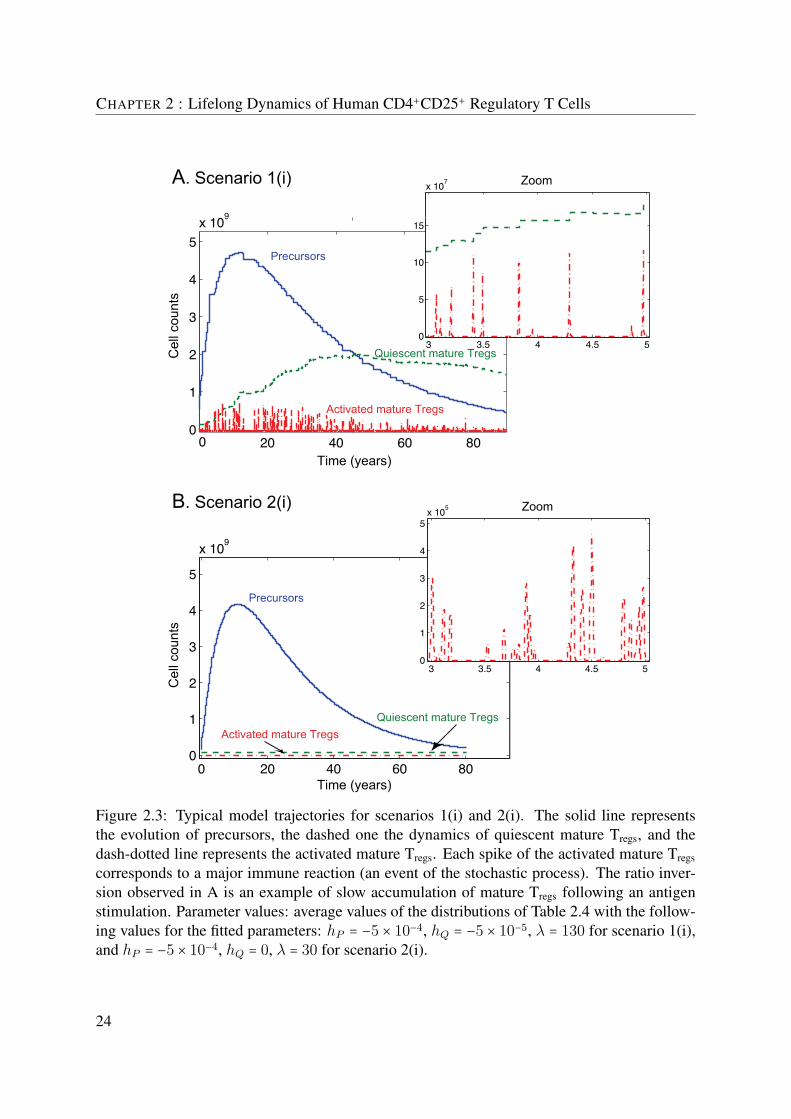
CHAPTER 2 : Lifelong Dynamics of Human CD4+CD25+ Regulatory T Cells
20 40 60 800
1
2
3
4
5
x 109
Time (years)
A. Scenario 1(i)
Precursors
Quiescent mature Tregs
Activated mature Tregs
0 20 40 60 800
1
2
3
4
5
x 109
Time (years)
B. Scenario 2(i)
Precursors
Quiescent mature TregsActivated mature Tregs
3 3.5 4 4.5 50
1
2
3
4
5x 10
5 Zoom
3 3.5 4 4.5 50
5
10
15
x 107 Zoom
0
Cel
l cou
nts
Cel
l cou
nts
Figure 2.3: Typical model trajectories for scenarios 1(i) and 2(i). The solid line representsthe evolution of precursors, the dashed one the dynamics of quiescent mature Tregs, and thedash-dotted line represents the activated mature Tregs. Each spike of the activated mature Tregs
corresponds to a major immune reaction (an event of the stochastic process). The ratio inver-sion observed in A is an example of slow accumulation of mature Tregs following an antigenstimulation. Parameter values: average values of the distributions of Table 2.4 with the follow-ing values for the fitted parameters: hP = −5 × 10⁻⁴, hQ = −5 × 10⁻⁵, λ = 130 for scenario 1(i),and hP = −5 × 10⁻⁴, hQ = 0, λ = 30 for scenario 2(i).
24

2.2 Materials and Methods
Proliferationscenarios
Proliferation capacity of... Parameter setting
Precursors Mature Tregs
1 Proliferate Proliferate aP > 0, aR > 0, dP > 02 Do not proliferate Do not proliferate aP = 0, aR = 0, dP = 03 Proliferate Do not proliferate aP > 0, aR = 0, dP > 04 Do not proliferate Proliferate aP = 0, aR > 0, dP = 0
Table 2.3: Definition of the four proliferation scenarios. Parameter meanings: aP , antigen-induced proliferation rate of precursors; aR, antigen-induced proliferation rate of mature Tregs;dP , antigen-induced death rate of precursors.
The model at a glance: typical model trajectories
In order to gain some insight into the model dynamics, we present in this section an ex-ample of execution of our model. Figure 2.3 shows the number of precursors (solid line) andmature Tregs (resting: dashed line and activated: dash-dotted line) as function of time in humanperipheral’s blood. The zoomed sections allow a closer look at the activated Tregs populationwhich is mainly present during major immune reactions, events of the stochastic process.
In Figure 2.3A is depicted a typical trajectory for scenario 1(i) where the ratio betweenprecursors and mature Tregs is inverted in the early years of adulthood, whereas in Figure 2.3Bis shown a typical trajectory for scenario 2(i) where the ratio inversion is not observed. Allmodel scenarios will be evaluated based on their capacity to reproduce this ratio inversion andon the capacity to reproduce the total amount of Tregs suggested by the data. Note that becausethe thymus produces thymocytes with a constant proportion of each subtype of Tregs, there arefour means of achieving a precursor/mature Tregs ratio inversion: 1) a difference in lifespans ofprecursors and mature Tregs; 2) a difference in the homeostatic proliferation rates of precursorsand mature Tregs; 3) the slow accumulation of mature Tregs following an antigen stimulation;4) an external source of mature Tregs. The first mean is present in all model scenarios andit acts in combination with the other three means. Thus in each model scenario, we observea combination of the above means and this combination can be sufficient or not to achievethe ratio inversion. For example, in Figure 2.3 where there is no homeostatic regulation, thelifespan of precursors is larger than the lifespan of mature Tregs (∣hP ∣ > ∣hQ∣), but this lifespandifference is not sufficient to achieve the ratio inversion. Here, the slow accumulation of matureTregs, present in scenario 1(i) and not in scenario 2(i), is needed.
Parameters
In order to cope with the large number of parameters and to decrease the effect of singlevalues on the dynamics of the model, we split the parameters in two groups: G1, parameters forwhich some a priori information is found, and G2, unknown parameters that must be fitted tothe data (see Section 2.2.2 for a detailed description of the data). The probability distributionof parameters of group G1 is defined in the following way: we find in the literature either aparameter together with a confidence interval accounting for the uncertainty of the estimation,or a finite range without any preferred value specified. In the former case, we use a Gaussian
25

CHAPTER 2 : Lifelong Dynamics of Human CD4+CD25+ Regulatory T Cells
distribution with mean and variance given by the confidence interval. In the latter case, we usea uniform distribution over the range.
Our in vitro assays have shown that the expansion rate aP of Tregs precursors is similarto the one of CD4+CD25− naive T cells and that the expansion rate aQ of activated matureTregs is 1.4 to 2 times lower than the expansion rate of precursors. To our knowledge, the invivo expansion rate of precursors (or even of CD4+CD25− naive T cells) in humans has notyet been measured. The in vivo T cell responses in mice have been quantified in (De Boeret al., 2003) which gives a first idea about the order of magnitude of parameters such as theproliferation and death rates of CD4+ T cells, as well as the duration of a T cell response. ForaP , we find in (De Boer et al., 2003) values in the range 1 - 1.7 per day, so we are samplingfrom an uniform distribution between 1 and 1.7 (day−1) (aP ∼ U(1,1.7)). We set aR = aP /K,where K takes two different values, 1.4 and 5, the latter being an extreme value representingthe case where mature Tregs have a very limited proliferating capacity compared to precursors.The value of the differentiation rate b of precursors into mature Tregs defines two settings: in thefirst, b ∼ U(1,10) (Burroughs et al., 2006) and in the second, we apply the constraint b ≤ aP ,thus b ∼ U(0.5,1). We will see that these settings give slightly different results. The activationrate of quiescent mature Tregs is set to half of the differentiation rate of precursors, i.e., f = b/2,because mature Tregs are anergic and thus slow to activate. The duration δn of the expansionphase is drawn from a Gaussian distribution N(7.65,0.72) (in vitro assay and (De Boer et al.,2003)). Both death rates dP and dR are considered as uniform U(1,2) because they shouldhave similar or higher values to the proliferation rates for system stability issues. It is knownthat ∼ 5 − 10% of all effector cells become long-lived memory cells. Thus, we set c = dR/9,which corresponds to 10% of the maximum value of the effector response. The death rate dQis distributed according to N(0.0013,0.0002) (De Boer et al., 2003).
The thymic input is calculated as follows. For the value of the total number of CD4+ T cellsoutput from the thymus of a newborn (σ0) and for the thymic involution rate (ν), we found thefollowing parameter settings in literature: σ0 = 1.98 × 10⁸ cells per day and ν = 0.024 per year(Marusic et al., 1998; Steinmann et al., 1985); σ0 = 4.48 × 10⁸ cells per day and ν = 0.05 peryear (Clark et al., 1999; Dutilh and De Boer, 2003). We therefore use an uniform distributionU(1×108,5×108) for σ0 and U(0.01,0.06) for ν to include the above settings in our simulations.The percentage of CD25+ cells among all CD4+ thymocytes (%CD25thymus) was measured tobe 1.3% in young children (unpublished data).
The proportion πn, n ∈ N, of cells that respond to a particular antigen is drawn uniformlybetween 10−7 and 10−4 cells (De Boer and Perelson, 1993). To estimate the total number of Tcells in human’s peripheral blood as a function of age, T (t), we use the fact that the mean bloodvolume of a healthy 70 kg individual is 5 liters (Feldschuh and Enson, 1977) and it containsabout 1011 T cells (Clark et al., 1999). We then use a function that maps age to the mean weightof individuals (CDC, 1988–1994; WHO, 2009).
The constant and density-dependent homeostatic proliferation and death rates (hP , hQ, ϕP ,ϕQ, α,QM ), as well as the infections occurrence rate (λ) and the external input from the thymus(pthymus) or from CD25− conversion (s), are fitted to the data. The time-unit of the model is 1day. Table 2.4 summarizes all parameter values and distributions.
26

2.2 Materials and Methods
Mea
ning(u
nits)
ValueorDistribution
Source
1.Exp
ansion
ofprec
urso
rs(1/day
)aP
∼U(1,1.7)
Biologica
lassum
ption,
DeBoe
ret
al.(20
03)
2.Exp
ansion
ofac
tivated
matureTregs
(1/day
)aR
=aP/1.4
oraR
=aP/5
Invitro
assay,
Burroug
hset
al.
(200
6)3.
Diff
eren
tiatio
nof
prec
urso
rs(1/day
)b∼U(1,10)
orU(0.5,1
)Burroug
hset
al.(20
06)
4.Restin
gof
matureTregs
(1/day
)c=dR/9
10%
ofresp
onse
peak
5.Dea
thof
prec
urso
rs(1/day
)dP
∼U(1,2
)Simila
rtoaP
6.Dea
thof
activ
ated
matureTregs
(1/day
)dR
∼U(1,2
)Simila
rtoaP
7.Dea
thof
quiescen
tmatureTregs
(1/day
)dQ
∼N
(0.001
3,0.00
02)
DeBoe
reta
l.(200
3)8.
Activationof
matureTregs
(1/day
)f
∼U(0.5,5
)or
f∼U(0.25,0.5)
Biologica
lassum
ption
9.Durationof
expa
nsionph
ase(day
s)δ∼N
(8,1.33)
Invitroassay
10.
Antigen
spec
ificity
πn∼U(10−7,10−
4)
DeBoe
rand
Perelson
(199
3)11
.Pr
obab
ility
ofprim
aryinfections
atbirth
K1∼U(0.7,1
)Biologica
lassum
ption
12.
Lim
itprob
a.of
prim
aryinfections
atad
ulthoo
dK
2∼U(0,0.4)
Biologica
lassum
ption
13.
Age
atwhich
theprob
a.of
prim
aryinfections
isha
lf(day
s)t h
∼U(10∗36
5,30
∗36
5)Biologica
lassum
ption
14.
Max
imum
declinerate
ofq(t)
ω∼U(0.01,0.5)
Biologica
lassum
ption
15.
Meanbloo
dvo
lumein
ahe
althy70
kgindividu
al(lite
rs)
5Fe
ldschu
han
dEns
on(197
7)16
.Num
bero
fTce
llsin
5lof
bloo
d(cells)
T5l∼U(1
×10
11,5
×10
11)
Clark
etal.(19
99)
17.
Num
berof
CD4+
cells
output
from
thethym
usof
ane
wbo
rn(cells/day
)σ0∼U(1
×10
8,5
×10
8)
Clark
etal.(199
9);Dutilh
and
DeBoe
r(200
3);M
arus
icet
al.
(199
8);S
teinman
net
al.(19
85)
18.
Thy
mic
invo
lutio
nrate
(1/day
)ν∼U(0.01/36
5,0.06
/365
)Clark
etal.(199
9);Dutilh
and
DeBoe
r(200
3);M
arus
icet
al.
(199
8);S
teinman
net
al.(19
85)
19.
%CD25
+inside
CD4+
cells
output
from
thethym
us%CD25
thym
us=0.00
65Data
20.
%CD25
+am
ongallT
cells
inco
rdbloo
d%CD25
cb∼N
(0.03,0.01
)Data
21.
Prop
ortio
nof
prec
urso
rsinside
CD4+
CD25
+in
cord
bloo
dpcb
∼N
(0.78,0.06
4)Data
22.
Prop
ortio
nof
matureTregs
inside
CD4+
CD25
+in
cord
bloo
dq c
b∼N
(0.21,0.06
4)Data
23.
Num
bero
fprecu
rsorsat
birth(cells)
P0=T(0
)∗%CD25
cb∗pcb
Data
24.
Num
bero
fmatureTregs
atbirth(cells)
Q0=T(0
)∗%CD25
cb∗q c
bData
Table2.4:
Apr
iori
parameter
distribu
tions
(param
etersof
grou
pG
1).
N(μ,σ)stan
dsforaGau
ssiandistribu
tionwith
meanμ
and
stan
dard
deviationσan
dU(a,
b)stand
sforaun
iform
distribu
tionon
[a,b
].Pa
rametershP,h
Q,λ
,ϕP,ϕ
Q,Q
M,α
,pthym
usan
dsare
fittedto
theda
ta.
27
CHAPTER 2 : Lifelong Dynamics of Human CD4+CD25+ Regulatory T Cells
2.2.2 Immunological data
Biological specimens
A transversal study was performed on the peripheral blood of 120 healthy subjects con-stituted by 60 males with a median age of 52.6 (range 20-81) and 60 females with a medianage of 49.32 (range 19-78). Samples of peripheral blood were obtained from laboratory co-workers or from the Blood Bank of the Centre Hospitalier Universitaire Vaudois, Universityof Lausanne, while the 7 samples of cord blood and the 2 thymuses were obtained from theDepartment of Clinical Chemistry, Microbiology and Immunology, University Hospital, Uni-versity of Ghent, Belgium. Cord and peripheral blood mononuclear cells were isolated usingstandard Ficoll-Hypaque (Amersham Pharmacia Biotech, Piscataway, NJ) gradients centrifu-gation. Blood specimens were collected under protocols approved by the Institutional ReviewBoards of the above mentioned Institutions.
FACS analysis and sorting
Cell surface analysis and sorting were performed using a combination of a panel of sur-face markers: PercP or PercP Cy5.5 conjugated mouse anti-human CD4 (Becton Dickinson,Franklin, NJ), APC-conjugated mouse anti-human CD25 (BD PharMingen, San Diego, CA),PE-conjugated mouse anti-human CD62L or PE-conjugated mouse anti-human CD71 (BectonDickinson, Franklin, NJ), FITC or PE-conjugated mouse anti-human CD45RO (BD PharMin-gen, San Diego, CA) and FITC Annexin-V (Becton Dickinson, Franklin, NJ). For cell-sortingexperiments CD4+CD25+CD62L+CD45RO−, CD4+CD25+CD62L+CD45RO+, CD4+CD25−-CD62L+CD45RO− and CD4+CD25−CD62L+CD45RO+ cell populations were isolated fromthe peripheral blood. The grade of cell purity in all the sorting experiments was more than97%. All flow cytometric analyses were performed on a FACS Calibur and cell sorting on aFACS Aria (Becton Dickinson Systems, Franklin, NJ). For intracellular FOXP3 analysis, cellpreparations were fixed and permeabilized with fixation/permeabilization buffers (eBioscience)after staining of cell surface markers and stained with FITC-conjugated rat antiñhuman FOXP3(eBioscience).
Regulatory T cells have been sorted and purified from peripheral and cord blood based ona CD4+CD25highCD62L+ gate. In order to analyze the purity of naturally occurring Tregs, theabove population has been stained for Foxp3. It is clear from Figure 2.4 that the cells sortedwith this method are in majority Foxp3 positive. CD4+CD25−CD62L+ cells have been sortedand stained in the same way. The majority of all CD25− cells are Foxp3 negative. Naturallyoccurring Tregs express CD25 constitutively and contrary to recently activated CD25− T cells,they do not downregulate this receptor. It is not excluded that the above sorting from peripheralblood involves some adaptive Tregs which are also included in the mathematical model presentedhereafter.
Suppression assay
Sorted purified CD4+CD25− T cells have been stimulated in vitro with anti-CD3 and anti-CD28 antibodies for 3 days alone (positive control) or in presence of sorted purified CD4+-
28

2.2 Materials and Methods
Figure 2.4: Isolation and characterization of human CD4+CD25+ Tregs from peripheral and cordblood. A. Representative flow cytometry profiles of one peripheral blood sample (1 out of 120).B. Representative flow cytometry profiles of one cord blood sample (1 out of 7). RegulatoryT cells have been sorted and purified from peripheral and cord blood based on the gate onCD4+CD25highCD62L+ cells; the gate for non-regulatory T cells was on CD4+CD25negCD62L+
cells. In both peripheral and cord blood, the majority of CD4+CD25+ cells are Foxp3+ and themajority of CD4+CD25− cells are Foxp3−.
CD25+CD62L+CD45RO+ T cells to test the suppressive function of the latter on the prolif-eration capacity of the former population. CD4+CD25+CD62L+CD45RO+ T cells have beenadded directly in the same well or in a transwell to test if their suppressive function needs cell-to-cell contact or is mediated by cytokines. CD4+CD25+CD62L+CD45RO+ T cells were ableto strongly suppress (96%) the proliferation of CD4+CD25neg T cells when co-cultured in thesame well, but lost all suppressive activity once cultured in a transwell (Figure 2.5).
Proliferation, activation and differentiation experiments
In order to assess the proliferation capacity, peripheral blood sorted cell populations (CD4+-CD25+CD62L+CD45RO−, CD4+CD25+CD62L+CD45RO+, CD4+CD25−CD62L+CD45RO− andCD4+CD25−CD62L+CD45RO+) were plated at 5×10³ cells per well in 96 U-bottomed plates inRPMI 1640 plus 10% FBS in the presence of 5×10⁴ irradiated (4000 rads) syngeneic peripheralblood mononuclear cells. Cells were cultured in the presence of soluble anti-CD3 (OKT3) plussoluble anti-CD28 (BD Pharmingen, San Diego, CA) with or without IL-2. The proliferationkinetic was followed by FACS over 15 days and by [3H]-Thymidine incorporation in corre-spondence of proliferative peaks. The activation and differentiation were monitored during 15days by the expression of activation markers such as CD25 and CD71 (Transferrin Receptor)and the marker of mature cells CD45RO. Cell death by apoptosis was measured in parallel foreach population by expression of Annexin-V.
29

CHAPTER 2 : Lifelong Dynamics of Human CD4+CD25+ Regulatory T Cells
Figure 2.5: Cell-to-cellcontact is needed by theCD4+CD25+CD62L+CD45RO+
T cells to exert their suppressivefunction, while cytokines do notseem to play any role.
Extrapolation of a mathematical model from empirical observations
Prior to formulating a mathematical model, we studied the proliferation kinetics of threepopulations (CD4+CD25+CD62L+CD45RO−, CD4+CD25+CD62L+CD45RO+, and CD4+CD25−-CD62L+CD45RO− cells) that may be involved in the maintenance of a constant pool of regula-tory T cells. The assay was performed several times using sorted cells from different subjectsin order to extrapolate some parameter values for the model, free from the individual vices.Each of the sorted cell populations was cultivated in presence of a polyclonal stimulus in orderto stimulate all the clones contained in a population. All the experiments were designed in sucha way that IL-2 is added at the beginning of the culture and every two days, because of thelimited proliferation capacity of mature Tregs. In fact, these cells did not show any apprecia-ble proliferation in other parallel experiments driven in the absence of IL-2. Each experimentlasted 15 days to permit the estimation of parameter values such as the duration of the prolif-eration phase, the amount of cells produced, the number of cells that were activated (CD71+),differentiated and acquired a mature phenotype (CD45RO+), the cell death (Annexin+ cells)and the number of surviving cells. We then studied retrospectively the distribution of the abovepopulations in the peripheral blood of 120 healthy individuals, 7 cord blood samples and 2thymuses, obtained from two children of 1 and 3 years old, who underwent cardiac surgery. Inthis way, we obtained the distribution of the above populations as a function of age.
2.2.3 Model evaluation procedure and parameter fitting
The model assessment procedure consists in the following steps: first, we consider themean model dynamics and we fit the unknown parameters to the biological data using a least-squares procedure (implemented in Matlab). The mean model is derived from the stochastic
30

2.2 Materials and Methods
one by fixing the parameters of group G1 to the mean value of their a priori distribution and byaveraging over the remaining random quantities. The latter are Yclone, the size of the respondingclone, andΔn = τn+1 − τn, the time-interval between two consecutive immune reactions. Basedon this fit, we can reject some model scenarios. However, this result may depend on the meanvalues of the a priori distributions. In order to eliminate this possibility, we fit the stochasticmodel (in which parameters of group G1 are random variables) using a Bayesian approach.This fit consists in maximizing the likelihood function, a measure of how good is the modelin explaining the data. It is the probability that, given the best-fit parameters and the a prioridistributions, the data is a realization of a particular model scenario. The higher this probability,the closer the model is to the data. The likelihood of a model scenario is computed as follows.
Consequently to the fact that the parameters of group G1 are defined as random variables,{P (t)}t∈R, {Q(t)}t∈R and {R(t)}t∈R are stochastic processes. In order to fit each model sce-nario to the biological data, we transform the above processes in the format of the data, i.e., interms of the ratio precursor/mature Tregs and of the percentage of CD4+CD25+ cells inside all Tcells, in logarithmic scale. Thus, we consider two other stochastic processes, namely {U(t)}t∈Rand {V (t)}t∈R, given by
U(t) ∶= log( P (t)Q(t) +R(t))
V (t) ∶= log(P (t) +Q(t) +R(t)T (t) ) ,
where T (t) is the total number of T cells at time t.Let gUV (u, v; t) be the joint density ofU and V . Because it is difficult to compute gUV (u, v; t)
analytically, we estimate it using Monte Carlo simulation, as follows. The model is executedM times for a time horizon of 85 years with parameters drawn according to the distributions ofTable 2.4. At each time, the density of trajectories in the space of U and V is estimated usinga bivariate histogram. Call g(s)UV (u, v; t) the estimated density of model scenario s at time t.Using the M model replicates, we construct a confidence interval for the bivariate histogramDavison (2003). We then consider the relative size of the confidence interval of each bin. If thelatter is greater than 10% for some bin, the number of replicates M is increased. The densityestimation is considered satisfactory if the relative size of the confidence interval of all bins issmaller than 10%. In the case of our model scenarios, M is taking values between 100 000 (inmost cases) and 500 000.
Each model scenario s is fitted to the data by maximizing the log-likelihood function definedas
s(θ) = N∑i=1
log (g(s)UV (ui, vi; θ∣ti)) , θ ∈ Θs,
where N is the number of data points (N = 126) and g(s)UV (ui, vi; θ∣ti) is regarded as a function
of θ for (ui, vi) and ti fixed. The parameter space Θs is defined by the values that can takethe free parameters θ = (hP , hQ, λ, ϕP , ϕQ, QM , α, pthymus, s). See Figure 2.6 for a visualexplanation of the likelihood computation.
The log-likelihood of is also used for objectively comparing the different model scenariosby performing a likelihood ratio test (F-test) for nested models that formally rejects the scenar-
31

CHAPTER 2 : Lifelong Dynamics of Human CD4+CD25+ Regulatory T Cells
uv −5
−3.5−2
−0.51
−7
−6
−5
−4
−3
−2
0
0.02
0.04
0.06
0.08
0.1
−5 −4 −3 −2 −1 0 1 2−7
−6.5
−6
−5.5
−5
−4.5
−4
−3.5
−3
−2.5
u
v
0
0.01
0.02
0.03
0.04
0.05
0.06
0.07
0.08
A
C
B Likelihood of a single data point (age: 54)
Likelihood of the entire data set
Estimated density
Time (years)
v
u
Figure 2.6: Likelihood computation under model scenario s. A: at each age ti, the densityg(s)UV (u, v; ti) of the model is estimated. u stands for the ratio precursor/mature Tregs and v, for
the percentage of CD4+CD25+ cells inside all T cells. B: the estimated density gUV (u, v; θ∣ti)of the model is used to compute the likelihood of each data point. In this example, the likelihoodof the point (u, v) = (−1.21,−4.41) (age: 54 years) is equal to 0.028. C: the log-likelihood ofthe entire data set is equal to the sum of the log-likelihoods of all data points.
ios that are not compatible with the data. Two models are nested if the parameter space of oneof them is a subset of the parameter space of the other. Proliferation scenarios 2, 3 and 4 (nullhypothesis) are subsets of scenario 1 and homeostasis scenario (i) (null hypothesis) is a subsetof all other homeostasis scenarios. The null hypothesis is rejected if the p-value of the test is< 0.01.
32
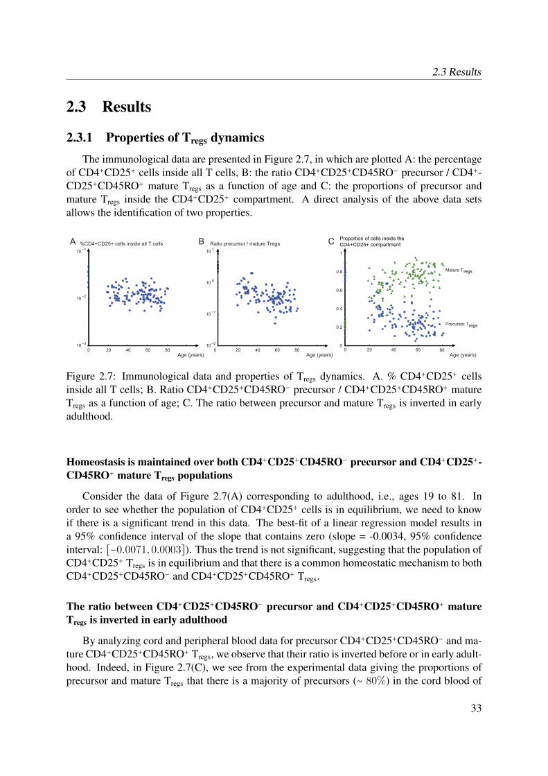
2.3 Results
2.3 Results
2.3.1 Properties of Tregs dynamics
The immunological data are presented in Figure 2.7, in which are plotted A: the percentageof CD4+CD25+ cells inside all T cells, B: the ratio CD4+CD25+CD45RO− precursor / CD4+-CD25+CD45RO+ mature Tregs as a function of age and C: the proportions of precursor andmature Tregs inside the CD4+CD25+ compartment. A direct analysis of the above data setsallows the identification of two properties.
%CD4+CD25+ cells inside all T cells
Age (years)
Ratio precursor / mature Tregs
Age (years)
A B
Age (years)
Proportion of cells inside theCD4+CD25+ compartment
0 20 40 60 8010 −2
10 −1
10 0
10 1
0 20 40 60 8010 −3
10 −2
10 −1
0 20 40 600
0.2
0.4
0.6
0.8
1
Mature T regs
Precursor Tregs
80
C
Figure 2.7: Immunological data and properties of Tregs dynamics. A. % CD4+CD25+ cellsinside all T cells; B. Ratio CD4+CD25+CD45RO− precursor / CD4+CD25+CD45RO+ matureTregs as a function of age; C. The ratio between precursor and mature Tregs is inverted in earlyadulthood.
Homeostasis is maintained over both CD4+CD25+CD45RO− precursor and CD4+CD25+-
CD45RO+ mature Tregs populations
Consider the data of Figure 2.7(A) corresponding to adulthood, i.e., ages 19 to 81. Inorder to see whether the population of CD4+CD25+ cells is in equilibrium, we need to knowif there is a significant trend in this data. The best-fit of a linear regression model results ina 95% confidence interval of the slope that contains zero (slope = -0.0034, 95% confidenceinterval: [−0.0071,0.0003]). Thus the trend is not significant, suggesting that the population ofCD4+CD25+ Tregs is in equilibrium and that there is a common homeostatic mechanism to bothCD4+CD25+CD45RO− and CD4+CD25+CD45RO+ Tregs.
The ratio between CD4+CD25+CD45RO− precursor and CD4+CD25+CD45RO+ mature
Tregs is inverted in early adulthood
By analyzing cord and peripheral blood data for precursor CD4+CD25+CD45RO− and ma-ture CD4+CD25+CD45RO+ Tregs, we observe that their ratio is inverted before or in early adult-hood. Indeed, in Figure 2.7(C), we see from the experimental data giving the proportions ofprecursor and mature Tregs that there is a majority of precursors (∼ 80%) in the cord blood of
33

CHAPTER 2 : Lifelong Dynamics of Human CD4+CD25+ Regulatory T Cells
newborns and a majority of mature Tregs (∼ 80%) in the peripheral blood of adult donors. Thisratio is inverted at latest in the early adulthood (20-30 years of age) and this inversion is whatwe call the "development of an in vivo pool of CD4+CD25+CD45RO+ mature Tregs". The fol-lowing results show that the ratio inversion is a critical issue that is not achieved by all modelscenarios.
2.3.2 Analysis of the mean model
In this section, we fit the mean model to the data of Figure 2.7. As a reminder, the meanmodel is derived from the stochastic one by fixing the parameters of group G1 to the meanvalue of their a priori distribution and by averaging over the remaining random quantities.
Figure 2.8 shows the trajectories of precursors (left subplots) and mature Tregs (right sub-plots) under the four proliferation scenarios. Parameters hP , hQ, λ, ϕP , ϕQ, QM , α, pthymus
and s are fitted to the data using a least squares procedure (see Table 4.3 for best-fit values andTable 2.6 for confidence intervals). The three different line types and colors in Figure 2.8 cor-respond to the three homeostasis scenarios: solid red, scenario (i) (density-independent regula-tion), dashed blue, scenario (ii) (density-dependent regulation) and dash-dotted green, scenario(iii) (external contribution). The dynamics of precursors are very similar for all scenarios: weobserve an increase during the first 10 years, followed by an exponential decrease. This is notsurprising as this population is mainly influenced by the influx of recent thymic emigrants. Themajor difference is in the dynamics of mature Tregs. This population increases constantly withage, but according to the studied scenario, we observe qualitative differences in the way thepopulation grows.
Before assessing the proliferation scenarios, we first wanted to see whether one or the otherhomeostasis scenario is better explaining the data. For this, we applied an F-test for nestedmodels opposing consecutively scenario 1(i) (H0) to scenarios 1(ii)a, 1(ii)b, 1(iii)a and 1(iii)b(H1). At level 0.01, H0 was not rejected. This suggests that we do not have a strong evidencethat a density-dependent homeostatic mechanism is regulating the population of mature Tregs.
The following three subsections describe the assessment results of the four proliferationscenarios, given either homeostasis scenario (i), (ii), or (iii).
In the case of a density-independent regulation of mature Tregs, the ratio inversion is a
critical issue if the peripheral differentiation of precursors is the only source of mature
Tregs
First note that due to the linearity of the differential equations of scenario (i), the ratio inver-sion can be achieved either because of a lifespan difference or through the slow accumulationof mature Tregs following an immune response. In what follows, we’ll see that the lifespandifference alone is not sufficient to achieve the ratio inversion.
From the solid red lines of the upper plots in Figure 2.8, we see that scenario 1(i) is achiev-ing the ratio inversion, whereas scenario 2(i) is not. The difference between these two scenariosis easy to explain when observing the typical trajectories of P , Q and R in Figure 2.3. Indeed,the magnitude of immune responses is very different in both scenarios (zoomed sections of Fig-ure 2.3). In scenario 1(i), the clonal expansion goes up to 107 cells, whereas in scenario 2(i), it
34

2.3 Results
Scenario 1 Scenario 2
Scenario 3 Scenario 4
0 20 40 60 8010
7
108
109
1010
Time (years)
Precursors
0 20 40 60 8010
7
108
109
1010
Time (years)
Mature Tregs
0 20 40 60 8010
7
108
109
1010
Time (years)
Precursors
0 20 40 60 8010
7
108
109
1010
Time (years)
Mature Tregs
0 20 40 60 8010
7
108
109
1010
Time (years)
Mature Tregs
Num
ber o
f cel
lsN
umbe
r of c
ells
Num
ber
of c
ells
Num
ber
of c
ells
Precursors
0 20 40 60 8010
7
108
109
1010
Time (years)
Precursors
0 20 40 60 8010
7
108
109
1010
Time (years)
Mature Tregs
0 20 40 60 8010
7
108
109
1010
Time (years)
Sc. (ii) b,(iii) a, b
Sc. (ii) a
Sc. (i)
Sc. (ii) a
Sc. (ii) b,(iii) a, b
Sc. (i)
Sc. (i)
Sc. (i)Sc. (ii) b,(iii) a, b
Sc. (ii) b,(iii) a, b
Sc. (ii) aSc. (ii) a
DataSc. (i)Sc. (ii) aSc. (ii) bSc. (iii) aSc. (iii) b
Sc. (i)
Sc. (i)
Data
Mean model dynamics(all scenarios)
Figure 2.8: Best-fit of the mean model with parameters of group G1 set to the mean values oftheir a priori distributions. Solid red: for scenario (i) (density-independent regulation); dashedblue: scenario (ii) (density-dependent regulation) and dash-dotted green: scenario (iii) (externalcontribution). Bold lines: sub-setting (a), light lines: sub-setting (b). The ratio inversionbetween precursor and mature Tregs is not achieved early enough in scenarios 2(i) and 3(i). Allother scenarios are able to explain the data.
does not exceed 105 cells. This has an impact on the size of the mature Tregs pool: in the caseof scenario 2(i), the only input to the mature Tregs population are the long-lived cells that havesurvived an immune reaction and they are set as 10% of the maximum effector response. Asthe peak of the effector response is relatively low, caused by the non-proliferating state of Tregs
in scenario 2(i), very few cells feed the mature Tregs pool. Therefore, in scenario 2, the onlyway to achieve a ratio inversion is through a difference in parameters hP and hQ because thereis a deficient accumulation of mature Tregs following an antigen response. The latter parametersbeing fitted, we see that scenario 2(i), even with positive values of hQ (Table 4.3) can not reachthe plateau level of the pool of mature Tregs suggested by the data. This suggests that, in thecase of a density-independent regulation of mature Tregs, the slow accumulation observed onlywhen there is a sufficient population expansion during antigen-triggered immune reactions isnecessary to achieve the ratio inversion.
A similar explanation is valid for scenario 3(i) in which only precursors are endowed witha proliferation capacity. This scenario seems to be unable to accumulate a sufficient pool ofmature Tregs (bottom left subplot of Figure 2.8). This is because for the mean values of theparameters of group G1 (Table 2.4), the differentiation rate b is on average larger than theproliferation rate aP , meaning that following an antigen priming, precursors have a higher
35

CHAPTER 2 : Lifelong Dynamics of Human CD4+CD25+ Regulatory T Cells
ScenarioBest-fit Parameters
hP hQ λ ϕP ϕQ QM α pthymus s(×10−5 (×10−5 (days) (×10−13 (×10−13 (×107 (day−1) (%) (×105
day−1) day−1) day−1cell−1) day−1cell−1) cells) cells)
1
(i) -7.83 -8.87 51.65 4.86(ii) a -4.42 60.53 58.98 3.27 2.54(ii) b 7.84 -18.20 99.44 4.41 7.50 0.0051(iii) a 7.10 -8.05 92.94 3.84 83.95(iii) b 14.35 -16.74 95.37 5.11 3.23
2
(i) -0.48 15.16 0.95 6.36(ii) a -4.69 156.40 60.88 3.23 5.55(ii) b 12.19 -16.61 164.80 4.87 2.04 0.0250(iii) a 6.54 -1.78 100.95 3.63 78.87(iii) b 12.22 -16.21 97.34 4.87 4.96
3
(i) -0.29 15.07 1.25 6.50(ii) a -4.75 203.77 55.39 3.22 7.23(ii) b 12.00 -17.35 168.80 4.85 6.02 0.0090(iii) a 6.55 -1.78 101.74 3.63 78.87(iii) b 12.52 -16.18 98.47 4.90 4.95
4
(i) -20.53 -5.97 63.57 1.48(ii) a -13.78 64.60 55.70 2.29 2.66(ii) b 12.15 -19.96 98.57 4.87 9.90 0.0045(iii) a 2.29 -7.96 91.78 3.29 81.87(iii) b 17.46 -16.98 92.24 5.42 3.43
Table 2.5: Best-fit parameters of the mean model dynamics for each model scenario.
probability of differentiating into hyporesponsive mature Tregs than to proliferate as precursors.Thus, most cells become anergic before having divided and the mature Tregs pool is underfed.As in scenario 2(i), a large and positive hQ (Table 4.3) is not able to make up for the lack ofaccumulation of mature Tregs following antigen priming. In order to eliminate any dependenceof this result to the exact values of the parameters of group G1, we will study the behavior ofscenario 3(i) in the stochastic model (Section 3.3).
Finally, the analysis of the mean model trajectory for scenario 4(i) suggests that the ratiocan be inverted (bottom right subplot of Figure 2.8). Note that this scenario is favored bythe fact that the rate of secondary infections increases with age. Secondary responses recruitmore mature Tregs that, once activated, start proliferating intensively. Therefore, the fact thatprecursors do not divide has only a minor impact on the population dynamics. However, wewill evaluate the performance of this scenario with the stochastic model in order to see how itis affected by a change in the proliferation parameter values.
36
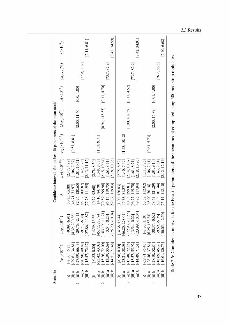
2.3 Results
Scen
ario
Con
fiden
ceintervalsforthe
best-fi
tparam
etersof
themea
nmod
el
hP(×
10−5)
hQ(×
10−5)
λϕP(×
10−13)
ϕQ(×
10−13)
QM
(×10
7)
α(×
10−2)
pthym
us(%
)s(
×10
5)
1
(i)
[-8.03
,-6.73
][-9.09
,-6.91
][50.75
,65.88
][2.47,
4.98
](ii)a
[-29
.61,
34.81]
[4.32,
230.36
][46.71
,73.97
][1.06,
7.37
][0.57,
8.81
](ii)b
[-27
.99,
66.43]
[-29
.76,
-2.41]
[82.96
,120
.65]
[1.01,
10.51]
[2.00,
11.40]
[0.0,1
.05]
(iii)
a[-20
.90,
49.82]
[-9.77
,-6.38
][85.39
,100
.87]
[1.42,
7.73
][77.9,
88.9]
(iii)
b[-15
.47,
72.17]
[-27
.86,
-11.87
][77.78
,111
.95]
[2.13,
11.12]
[2.11,
6.01
]
2
(i)
[-0.83
,0.00]
[14.39
,16.66
][0.79,
93.60]
[2.78,
8.50
](ii)a
[-23
.42,
43.02]
[45.72
,273
.74]
[14.16
,84.70
][1.48,
8.33
][1.53,
9.71
](ii)b
[-15
.26,
72.00]
[-18
3.19
,-11
.71]
[79.59
,299
.96]
[2.15,
10.64]
[0.94,
415.55
][0.11,
4.70
](iii)
a[-13
.59,
55.69]
[-3.54
,-0.23
][95.15
,119
.75]
[1.61,
8.71
][73.7,
82.9]
(iii)
b[-14
.51,
71.48]
[-12
5.20
,-10
.04]
[52.07
,119
.03]
[2.18,
10.86]
[3.42,
34.59]
3
(i)
[-0.96
,0.00]
[14.38
,16.44
][1.00,
120.83
][2.75,
8.52
](ii)a
[-23
.21,
38.08]
[46.20
,278
.01]
[5.33,
81.37]
[1.40,
7.49
][1.53,
10.12]
(ii)b
[-15
.48,
72.15]
[-17
2.93
,-11
.55]
[80.85
,299
.81]
[2.14,
10.67]
[1.00,
407.59
][0.11,
4.52
](iii)
a[-13
.57,
55.92]
[-3.54
,-0.22
][96.77
,119
.70]
[1.61,
8.71
][73.7,
82.9]
(iii)
b[-14
.49,
71.51]
[-12
3.99
,-10
.04]
[49.76
,117
.94]
[2.18,
10.86]
[3.42,
34.91]
4
(i)
[-28
.91,
-6.46]
[-8.80
,1.19]
[53.58
,112
.02]
[1.11,
2.86
](ii)a
[-28
.46,
37.84]
[6.25,
153.84
][45.90
,70.18
][1.06,
7.41
][0.61,
5.73
](ii)b
[-28
.10,
52.84]
[-30
.37,
-0.62]
[78.67
,121
.29]
[1.01,
9.10
][2.00,
15.89]
[0.01,
1.00
](iii)
a[-18
.69,
45.37]
[-9.59
,-5.96
][83.93
,101
.44]
[1.43,
7.81
][76.2,
86.8]
(iii)
b[-16
.01,
80.73]
[-30
.05,
-12.50
][75.17
,118
.10]
[2.12,
12.14]
[2.40,
6.68
]
Table2.6:
Con
fiden
ceintervalsforthe
best-fi
tparam
etersof
themeanmod
elco
mpu
tedus
ing50
0bo
otstrapreplicates.
37

CHAPTER 2 : Lifelong Dynamics of Human CD4+CD25+ Regulatory T Cells
In presence of a density-dependent homeostatic regulation of mature Tregs, the ratio pre-
cursor/mature Tregs is inverted without the need of peripheral proliferation in response to
antigen.
This claim is suggested by the best-fit of homeostasis scenario (ii), where the populationsize is regulated either via a density-dependent death (sub-setting (a), bold dashed lines inFigure 2.8), or via a density-dependent homeostatic proliferation (sub-setting (b), light dashedlines in Figure 2.8). We see that both mechanisms produce different dynamics, but the lack ofdata in the age-range 0-19 years does not allow us to eliminate neither of them. The sum ofsquared errors indicates however that a density-dependent homeostatic renewal (scenario 1(ii)b)fits slightly better the data. This is not surprising as this scenario has one more parameter thanscenario 1(ii)a.
It is interesting to observe that a density-dependent death is compensating for a large andpositive value of hQ (Table 4.3) meaning that the turnover rate of the mature Tregs populationis very high. Concerning the density-dependant homeostatic renewal, we see from Table 4.3that the per cell maximal renewal rate α needs to be on average 2 times larger in the case ofhyporesponsiveness to antigen stimulation (scenario 2(ii)b) compared to the case where cellsproliferate (scenario 1(ii)b). Therefore we conclude that the density-dependent regulation isable to explain the data as long as there are no restrictions in the parameters defining the home-ostatic proliferation and death rates.
The ratio inversion is easy to achieve if there is an exponentially decreasing thymic output
or a constant external input to the mature Tregs population
This can be seen by analyzing the performance of homeostasis scenarios (iii)a and b. Thegreen dash-dotted lines in Figure 2.8 show the best-fit of these scenarios to the data (bold:scenario (iii)a, thymic output of mature Tregs; light: scenario (iii)b, external source). The ratioprecursors/mature Tregs is inverted regardless the underlying proliferation scenario. Althoughthere is no density-dependent regulation here, the increase of the population of mature Tregs isdue to the thymic output of mature Tregs (sc. 1-4(iii)a) or to the external and constant inputof mature Tregs (sc. 1-4(iii)b) from a phenotype switching of CD4+CD25− T cells. Thus, weconclude that in this case, the peripheral proliferation of precursor or mature Tregs is not requiredfor the development of the mature Tregs pool.
Furthermore, by analyzing the best-fit parameters of scenarios 1-4(ii)a (Table 4.3), we seethat on average, the estimated value of pthymus is about 80%. This means that the data canbe explained with 20% of all CD4+CD25+ T cells that exit the thymus having a CD45RO+
mature profile. Assuming that there are 1.3% CD4+CD25+ Tregs inside all CD4+ T cells exitingthe thymus, 20% (mature Tregs) of all Tregs is equivalent to 0.26% of all CD4+ T cells. Thus,if as few as 0.26% of all CD4+ T cells exiting the thymus are mature Tregs, antigen-drivenproliferation in periphery is no longer necessary for the deployment of the pool.
2.3.3 Analysis of the stochastic model
The analysis of the mean model led to the rejection of model scenarios 2(i) and 3(i). How-ever, this is true for the mean values of the a priori distributions, but it might not be true for
38

2.3 Results
all parameter values. To eliminate this possibility, we fit the stochastic model with parametersof group G1 sampled from the distributions in Table 2.4. We apply this only to homeostasisscenario (i), as the other homeostasis scenarios were able to explain the data already with themean model.
aP (day−1) aR (day−1) b (day−1)
Parameter setting 1 U(1,2) aR = aP /1.4 U(1,10)Parameter setting 2 U(1,2) aR = aP /1.4 U(0.5,1)Parameter setting 3 U(1,2) aR = aP /5.0 U(0.5,1)
Table 2.7: Parameter values and distributions of the three parameter settings. U(a, b) stands fora uniform distribution on [a, b].
In order to obtain results that are robust with respect to parameter values, we define threeparameter settings (Table 2.7) that give slightly different results. These settings concern threeimportant parameters of the immune response: aP , the proliferation rate of precursors, aR,the proliferation rate of activated mature Tregs and b, the differentiation rate of precursors intomature Tregs. In the first parameter setting of Table 2.7, the average value of b is larger thanthe average value of aP , in other words, precursors have a higher probability of acquiring themature phenotype than to proliferate as precursors in response to a foreign antigen. In settings 2and 3, it is the opposite: precursors stay longer (and possibly proliferate) in this undifferentiatedstate before acquiring the mature phenotype. In settings 1 and 2, aR takes values 1.4 timessmaller than the values of aP as measured in vitro, whereas in setting 3, we model an extremecase where mature Tregs proliferate, but 5 times less than precursors. Note that the analysis ofthe mean model in Section 3.2 was done under parameter setting 1.
To give an idea of the spread of trajectories of the stochastic model, Figure 2.9 shows thebest-fit of the stochastic model under scenarios 1-4(i) (parameter setting 1). In what follows,we use the evaluation procedure described in the Methods to assess all proliferation scenariosand find those that are unable to explain the biological data.
In the absence of a density-dependent homeostatic regulation, and of an external source
of CD4+CD25+CD45RO+ mature Tregs, proliferation of precursors, or of mature Tregs, is
necessary to the development of the mature Tregs pool
The result given hereafter is obtained in the case where the unique source of mature Tregs isthe peripheral differentiation of precursors without density-dependent homeostatic regulation(scenario (i)). The results of the model evaluation procedure applied to the four proliferationscenarios are shown in Figure 2.10A (see Table 2.8 for the best-fit parameters of the stochasticmodel). Each bar of Figure 2.10 indicates the absolute value of the maximum likelihood of aproliferation scenario. The closer this bar is to zero, the better the model is explaining the data.
We observe that scenario 2(i), i.e., the one in which neither precursors nor mature Tregs
proliferate, has a very poor performance in all three settings of Table 2.7. As stated in theprevious section, the problem with this scenario is its inability to achieve the ratio inversion.Indeed, we found no parameter values such that this scenario is explaining the data. Scenario
39

CHAPTER 2 : Lifelong Dynamics of Human CD4+CD25+ Regulatory T Cells
)i(2 oiranecS)i(1 oiranecS
)i(4 oiranecS)i(3 oiranecS
%CD4+CD25+ inside all T cells %CD4+CD25+ inside all T cells
%CD4+CD25+ inside all T cells%CD4+CD25+ inside all T cells
Ratio precursor/mature T regs
Ratio precursor/mature T regs
Ratio precursor/mature T regs
Ratio precursor/mature T regs
0 20 40 60 8010
-3
10-2
10-1
100
Time (years)
20%50%20%
DataMedian
0 20 40 60 8010
-2
10-1
100
101
102
Time (years)0 20 40 60 80
10-3
10-2
10-1
100
Time (years)0 20 40 60 80
10-2
10-1
100
101
102
Time (years)
0 20 40 60 8010
-3
10-2
10-1
100
Time (years)0 20 40 60 80
10-2
10-1
100
101
102
Time (years)0 20 40 60 80
10-3
10-2
10-1
100
Time (years)0 20 40 60 80
10-2
10-1
100
101
102
Time (years)
Figure 2.9: Distribution of model’s trajectories for scenarios 1(i)-4(i), parameter setting 1, fittedto the data. As the parameters are drawn from probabilistic distributions, every execution ofthe dynamical system is performed with different parameter values and the trajectories differ.Therefore, instead of a single trajectory, we have a distribution of trajectories. Solid red line:median. 50% of the trajectories are comprised between the 25% and 75% quantiles (dark greyzone); 40% of all trajectories are in the light grey zone, delimited by quantiles 5-25% and75-95%.
2(i) is therefore rejected when compared to scenario 1(i) using the F-test for nested models(in all parameter settings). This implies that the proliferation of precursors and of mature Tregs
following a successful interaction with an antigen presenting cell is essential to the developmentof a stable pool of mature Tregs in the absence of a density-dependent homeostatic regulationand of an external source of CD4+CD25+CD45RO+ regulatory T cells.
Now, in order to test which proliferating capacity is more important, the one of precursorsor the one of mature Tregs, we fit the stochastic model scenarios 3(i) and 4(i).
The proliferation of precursors alone is sufficient if E[b] < E[aP ]Figure 2.10A shows the results of the evaluation procedure applied to scenario 3(i) (light
grey bars) in which only precursors are endowed with a proliferation capacity. We remark that,as suggested by the assessment of the mean model, this scenario performs poorly in parameter
40

2.3 Results
Figure 2.10: Goodness of fit of themathematical model in scenario (i)(no homeostatic regulation). The barplot shows the absolute value of thelog-likelihood of each model sce-nario (black bars:proliferation sce-nario 1, dark grey: prolif. sce-nario 2, light grey: prolif. sce-nario 3, white: prolif. scenario 4).The closer the bar is to zero, thebetter the model fits the data. Foreach homeostasis scenario, we com-pare proliferation scenario 1 to allthe others by applying a hypothesistest for nested models. A significantdifference indicated by ** (p-value< 0.01) means that the consideredscenario is rejected.
Homeostasis Scenario (i)
HomeostasisScenario (i)
(maintenancesetting)
A B
Param. setting 2
Param. setting 1
Param. setting 3
1 2 3 4 1 2 3 4 1 2 3 4 1 2 3 40
100
200
300
400
500
600
|Max
. lik
elih
ood|
**** ****
**
Homeo.scenario
Prolif.scenario
Parametersetting
Best-fit Parameters
hP (×10−5) hQ(×10−5) λ ϕP (×10−13)
(i)
11 -20.00 -5.00 55.22 1.972 -0.12 -17.00 60.90 2.653 -0.18 0.00 6.76 5.72
21 -0.50 8.00 0.67 2.602 -0.50 1.00 1.80 5.303 -0.50 1.00 1.80 5.30
31 -1.00 11.00 5.27 4.782 -1.00 5.00 5.28 4.813 -1.00 5.00 5.28 4.81
41 -9.00 -8.00 20.00 2.002 -0.94 -0.93 22.66 4.453 -0.50 1.00 0.70 4.80
Mainte-nance(i)
1
1
-0.45 -0.11 200.00 4.072 -0.43 1.00 0.53 4.003 -0.43 1.00 0.53 4.004 -0.57 -1.00 130.00 4.00
Table 2.8: Best-fit parameters of the stochastic model for scenario (i) and all parameter settings.
41

CHAPTER 2 : Lifelong Dynamics of Human CD4+CD25+ Regulatory T Cells
setting 1. However, using the stochastic model, we have found two other parameter settings (2and 3) for which scenario 3(i) performs similarly to scenario 1(i). Thus, the stochastic modelsuggests that there exist parameter values for which the proliferation of precursors alone is suf-ficient to the development of a viable pool of mature Tregs. As a consequence, the F-test fornested models rejects scenario 3(i) only in parameter setting 1. The difference between param-eter setting 1 and parameter settings 2 and 3 being in the average value of the differentiationrate b with respect to the value of the proliferation rate of precursors aP , we conclude that inorder to validate model scenario 3(i), it must be shown that the proliferation rate aP of precur-sor cells is significantly larger than the rate b of expression of CD45RO following an antigenstimulus.
The proliferation of mature Tregs alone is sufficient if their division rate is not too small
compared to the division rate of precursors
The assessment of model scenario 4(i) in which only mature Tregs proliferate is illustrated inFigure 2.10A (white bars). For settings 1 and 2, the performance of this scenario is comparableto the one of scenario 1(i), whereas for parameter setting 3, scenario 4(i) is not able to reproducethe dynamics of the data and the maximum likelihood is fairly low. In that case, the F-testfor nested models rejects scenario 4(i) when compared to scenario 1(i). We remark that thishappens in the extreme case where mature Tregs proliferate very little (the distribution of aR inparameter setting 3 is U(1/5,1.7/5)). Thus, the proliferation of mature Tregs is sufficient for thedevelopment of a peripheral pool only if the proliferation rate is not too small.
2.3.4 Maintenance of a lifelong in vivo pool of CD4+CD25+CD45RO+ ma-
ture Tregs
In order to assess the importance of antigen-driven proliferation in the lifelong maintenanceof a peripheral pool of Tregs, we examine the situation where the model is executed from the timeat which the pool is already constituted, i.e., from the age corresponding to our first adulthooddata (19 years old). We only study here homeostasis scenario (i), as it is the only one that ledto the rejection of some proliferation scenarios.
Given that at the age of 20, a peripheral pool of mature Tregs is constituted, antigen-driven
proliferation in the periphery is not necessary for the maintenance even in the absence of
other input of mature Tregs or of a density-dependent homeostasis mechanism
We assess the four proliferation scenarios of Table 2.3, in the case of homeostasis scenario(i). The percentage of precursors inside CD4+CD25+ T cells at the age of 19 (p19) is drawnfrom a Gaussian distribution with mean 0.35 and standard deviation 0.1, values obtained fromthe statistics of the data points corresponding to the age range 19–24 years. The percentageof mature Tregs at the age of 19 is set to 1 − p19. The maximum likelihood of the fit of thestochastic model under all proliferation scenarios is in Figure 2.10B. None of the scenarios isrejected after the likelihood ratio test. Thus, the proliferation in response to antigen stimuli isnot necessary for the lifelong maintenance of a pool of mature Tregs, once the pool is constituted.
42

2.3 Results
2.3.5 Summary
All our findings are displayed in Table 2.9.
Biological
process
Findings Found
with
Propertiesof Tregs
dynamics
1. Homeostasis is maintained over both CD4+CD25+-CD45RO− precursor and CD4+CD25+CD45RO+ matureTregs populations.
Data
2. The ratio between CD4+CD25+CD45RO− precursor andCD4+CD25+CD45RO+ mature Tregs is inverted in earlyadulthood.
Data
3. The inversion of the ratio precursor/mature Tregs is easy toachieve in the presence of a density-dependent homeostaticmechanism of the mature Tregs population. In this case,there is no need of proliferation in response to immunogenstimulation.
Model
4. The ratio inversion is easy to achieve if there is a thymic ora constant external input to the mature Tregs population.
Model
Developmentof thematureTregs pool
5. In the absence of a density-dependent homeostatic regula-tion and of an external source of CD4+CD25+CD45RO+
mature Tregs, proliferation of precursors or of mature Tregs
is necessary to the development of the mature Tregs pool.
Model
6. The proliferation of precursors alone is sufficient if the pro-liferation rate of precursors is significantly larger than therate of acquisition of CD45RO following an immunogenstimulus.
Model
7. The proliferation of mature Tregs alone is sufficient if theirdivision rate is not too small compared to the division rateof precursors.
Model
Maintenanceof the ma-ture Tregs
pool
8. Given that at the age of 20 a peripheral pool of mature Tregs
is constituted, antigen-driven proliferation in the peripheryis not necessary for the maintenance even in the absence ofother input of mature Tregs or of a density-dependent home-ostasis mechanism.
Model
Table 2.9: Summary of all findings.
43

CHAPTER 2 : Lifelong Dynamics of Human CD4+CD25+ Regulatory T Cells
2.4 Discussion
With the help of a mathematical model, we studied different developmental pathways ofregulatory T cells and established conditions in which each of them can explain the biologicaldata. The stochastic infection process combined with the differential equations with randomparameters and Monte Carlo simulation is a modeling methodology allowing the description ofcell dynamics on the scale of years. We believe that such a scheme is particularly appropriatefor use in human studies, where data is sparse and several sources of uncertainty and noisehave an influence on parameter values. Although still requiring the computation of confidenceintervals, using random parameters was a way of avoiding tedious high-dimensional parameterfitting by decreasing the number of unknown parameters and instead, introducing distributionscovering an entire set of possible values. In order to keep the model tractable, we have madeseveral simplifying assumptions. One of them is the assumption that, except for thymic invo-lution, parameter distributions are independent on age. This is probably a simplification, butrecent studies indicate that CD4+CD25+ Tregs in aged mice are functionally comparable to thosein young mice (Nishioka et al., 2006).
In an effort to keep the model simple, we used a two-phase model (Eq. (2.1) and Eq. (2.3))that describes the way cells respond to antigen stimulus when only the responder cell populationis considered (Althaus et al., 2007; De Boer et al., 2003). Such a model corresponds to a viewof the immune system where the size of immune responses is proportional to the number ofpre-existing cells. However, the biological reality might be more complicated and it could bepossible that the number of cells produced at the end of an immune response is independent ofthe initial number of cells.
We have observed that the number of CD4+CD25+CD45RO− precursor Tregs decreases withage. This result confirms the findings of Valmori et al. (2005), where the authors point out asignificant negative correlation between the number of precursors and the age of donors. Then,we have observed that the number of CD4+CD25+CD45RO+ mature Tregs increases with age.This finding as well goes in the direction of the results of Valmori et al. (2005) and is in accor-dance with the results of Gregg et al. (2005), where the authors observe an increased number ofperipheral CD4+CD25hi T cells. We then have shown that the ratio between precursors and ma-ture Tregs is inverted in early adulthood. Furthermore, the model suggested the continuous-timetrajectory of Tregs. In particular, we have observed interesting cell dynamics during infancy andpuberty, time-periods for which we have not found immunological data due to ethical reasons.As this is the period of life where the thymus functions at a maximal regime, we have observedan important increase of thymus-derived precursor cells, peaking at 10-12 years old, age cor-responding to the onset of puberty. Then, precursor cells start their decline, while mature Tregs
continue their progressive increase, having their most important increase rate in the age range0-20 years. The latter is thus a critical period for the constitution of a pool of mature Tregs. Thisratio inversion was also a critical issue of the model behavior; it led to the elimination of somemodel scenarios that could not reproduce it.
We have studied several pool-size regulation mechanisms of Tregs: density-independent anddensity-dependent renewal/death of mature Tregs, as well as a constant or time-dependent ex-ternal contribution. Given these distinct mechanisms, we have identified conditions in whichthe antigen-driven proliferation is necessary for the creation of a viable pool of CD4+CD25+-
44

2.4 Discussion
CD45RO+ Tregs. It turned out that the antigen-driven proliferation is not necessary if a density-dependent homeostatic mechanism regulates the pool of mature Tregs. In other terms, as wefound no information about the exact values of the parameters governing the homeostaticregulation, the antigen-driven cell division could be replaced in our model by a homeostatic(cytokine-driven) proliferation. However, the homeostatic expansion is unlikely to be the mainsource of mature Tregs, because if that was the case, the diversity of the T cell receptor (TCR)repertoire would be reduced by competitive exclusion. Indeed, if there is no external contri-bution to this cell population, the diversity of T cell receptors would be determined by thefew cells present at birth. Yet, it is known that Tregs have an αβ TCR repertoire with size anddiversity closely similar to those of CD4+CD25- T cells (Fazilleau et al., 2007). Therefore,we believe that in addition to a homeostatic mechanism, other sources of de novo generationshould be present.
In that perspective, we have studied other sources of mature Tregs that are able to replenishthe peripheral pool of mature CD4+CD25+CD45RO+ Tregs and enrich the TCR repertoire. Onesuch source is the thymus output of mature Tregs. We have established the percentage of Tregs
that should be output daily from the thymus so that the peripheral expansion of this populationis not required for a successful development of the pool. This threshold is about 20% of allCD4+CD25+ T cells output from the thymus, or, equivalently, less than 0.3% of all CD4+ Tcells exiting the thymus. Another question arises then: are Tregs with a mature phenotype ableto exit the thymus? We found two points of view in the literature.
On the one hand, Wing et al. (Wing et al., 2003) claim that only regulatory T cells with anaive phenotype, namely CD45RO- precursors, are released in the periphery from the thymus(corresponding to our homeostasis scenario (i)). If this is indeed the case, then we have demon-strated that proliferation of both CD4+CD25+CD45RO− and CD4+CD25+CD45RO+ cells issufficient, but not necessary for the development and maintenance of a pool of Tregs. In sce-nario 3(i), where only precursors proliferate, we saw that if the differentiation rate of CD4+-CD25+CD45RO− precursors into CD4+CD25+CD45RO+ mature Tregs is similar to or greaterthan the proliferation rate of precursors, the model cannot explain the data. However, it isunlikely that precursor cells stop suddenly their proliferation because of the acquisition of themature phenotype. Our in vitro experiments have shown that in presence of antigen with aco-stimulatory signal, precursor CD4+CD25+CD45RO− cells proliferate intensively while ac-quiring the memory phenotype (unpublished data). This observation suggests that either theacquisition of CD45RO is not associated with anergy during a first priming, in which case,instead of scenario 3(i), scenario 1(i) would be the appropriate model, or the parameters gov-erning cell dynamics have the property that the rate of proliferation of precursors is greaterthan the rate of differentiation into mature Tregs, in which case scenario 3(i) is in accordancewith the in vivo data. In scenario 4(i), where only activated recently-matured CD4+CD25+-CD45RO+ cells proliferate, cells start their intense proliferation after a time-delay, which iscompatible with the fact that regulatory T cells activate slowly, only when there is a sufficientamount of growth resources in the environment. The fact that the expansion of regulatory Tcells is dependent on growth factors produced by other cells was also pointed out in (Burroughset al., 2006; León et al., 2000) . A recent study (Lee et al., 2008) brings light to the molecularmechanisms through which Foxp3 maintains the unresponsiveness of Tregs. The link of Foxp3to c-Jun blocks proliferation and therefore makes it even more difficult for Tregs to activate and
45

CHAPTER 2 : Lifelong Dynamics of Human CD4+CD25+ Regulatory T Cells
proliferate. Scenario 4 with its initial delay, attests for this difficulty.On the other hand, it cannot be excluded that a small proportion of mature-type Tregs might
exit thymus tissues. Vanhecke et al. (1995) identify five stages of thymocyte differentiationduring which CD4+ T cells acquire and lose several surface receptors. The last two stagesdefine the most mature cells that consist of CD4+CD1−CD45RO+ (stage 4) and CD45RO−
(stage 5) helper T cells. As no particular sorting was applied to mark regulatory T cells inthis study, we can assume that they are comprised in the above populations. Vanhecke et al.(1995) claim that both stage 4 and stage 5 cells emigrate from the thymus in a severe combinedimmunodeficient mouse carrying a human thymus, even though they consider CD45RO- stage5 cells as more mature. Another question arises then, which is whether these thymic emigrantswith mature profile switch back to a naive form soon after their entry in the periphery or not.This event was not considered in our mathematical model, but it will certainly reinforce theneed of proliferating capacity of Tregs for the development of a reliable pool. However, if thesestage 4 CD45RO+ Tregs maintain the mature profile once in the periphery, their number couldbe sufficient for the development of a pool of mature Tregs.
Recent studies point out the presence of an input of mature Tregs coming from non-regulatoryhelper T cells (Vukmanovic-Stejic et al., 2006). This hypothesis is perfectly able to explainthe biological data, when daily there are at least 105 CD4+CD25− cells acquiring a regula-tory profile. To our knowledge, there is no quantitative data measuring this transformation,nonetheless, we hypothesize that this external contribution should be such that the entire poolof CD4+CD25+FoxP3+ cells, including naturally occurring thymus-derived Tregs, is in steadystate, as suggested by our data.
At last, we have shown that although the antigen-driven proliferation of regulatory T cellsis essential for the development of a pool of mature Tregs, it is not a critical issue for the lifelongmaintenance of this compartment. This finding confirms the intuitive fact that the homeostasis-related kinetics have more impact on the lifelong maintenance of a cell population than theantigen-response kinetics.
An important contribution of the mathematical model described here is the suggestion ofnew research directions that will deepen our knowledge about regulatory T cells. Indeed, ourresults led to the identification of crucial mechanisms having an important impact on Tregs
dynamics and that could be subject to further investigations: the quantitative assessment of theparameters governing the homeostatic maintenance of Tregs, the assessment of the quantity ofmature Tregs exiting the thymus, and the quantitative description of the phenomena transforminga non-regulatory cell into a regulatory CD4+CD25+FoxP3+ T cell in vivo.
In conclusion, the mathematical model allowed us to have a global view on the lifelongdynamics of Tregs. We evaluated three different homeostatic scenarios about possible sourcesof mature Tregs that can explain how a stable pool of Tregs is developed and maintained throughhuman life. This enabled us to appreciate and estimate the different contributions of eachsingle path in the absence of others. Moreover, we also evaluated four different scenariosconcerning the intrinsic proliferation ability of precursors and mature Tregs. This ability has aconsiderable impact on Tregs development and maintenance if precursors are the unique sourceof mature Tregs. Our model is the first attempt to mathematically and computationally describethe behavior of regulatory T cells over life. The mathematical model is able to estimate thetrend of Tregs over time when one or more sources are affected. Although it is already possible
46
2.4 Discussion
to have an empirical idea of the future trend of regulatory T cells from the blood of a patient,it is not possible to predict their amount at a certain time in the future. Further developmentscould allow our in silico model to virtually monitor and predict the dynamics of regulatoryT cells through an individual life. This application can be particularly useful for prospectivestudies on patients that received a solid organ transplant or are suffering from an autoimmunedisease. Such patients have often decreased numbers of Tregs in their blood when compared tohealthy donors. Once the mathematical model is able to predict the amount of Tregs over time,it would allow to individually dose the immunosuppressive drugs needed to prevent chronicrejection episodes or disease relapses. In the perspective of introduction of regulatory T cells incell-therapy as a more specific and sophisticated substitute to immunosuppressive drugs (Rileyet al., 2009), our model is a first step towards the development of tools aiming the clinicalmonitoring of regulatory T cell dynamics before and after their adoptive transfer.
47

CHAPTER 2 : Lifelong Dynamics of Human CD4+CD25+ Regulatory T Cells
48

Chapter 3Analysis of the Tregs Model
In this chapter are given theoretical results related to the model of regulatory T cells pre-sented in Chapter 2. In Section 3.1, we obtain an analytical expression of the dynamical systemin question by solving the differential equations Eq. (2.1), Eq. (2.3) and Eq. (2.3) in the par-ticular case where these are linear (in the absence of homeostasis). In the following section(Section 3.2), we present the detailed computation of the mean dynamics, again in the absenceof homeostasis. Finally, in Section 3.3, we describe how is estimated the density of modeltrajectories, needed to compute the maximum likelihood of a scenario.
3.1 Generic model solution
In this section, we consider the Tregs model under homeostasis scenario (i), i.e., wherethere is no competition between cells for a common resource, nor fratricide. In this case,gQ(t) = 0, sQ = 0, ϕQ = 0, α = 0 and the ODE system of Eq. (2.3) is linear. As the ODEsdescribing immune responses are linear as well, we can easily solve the generic model. To dothat, we write the differential equations corresponding to the nth immune reaction at time τn inmatrix form:
dYclone(t)dt
= ⎧⎪⎪⎨⎪⎪⎩A Yclone(t) if τn ≤ t ≤ δ
B Yclone(t) if δ ≤ t ≤ τn+1, (3.1)
where
A = ⎛⎜⎝aP − b 0 0
0 −f 0b f aR
⎞⎟⎠ and B = ⎛⎜⎝−dP 0 00 −dQ c0 0 −(c + dR)
⎞⎟⎠are respectively the matrices defining the expansion and contraction phases of the immunereaction. Solving Eq. (3.1) for t ∈ [τn, τn+1] yields:
Yclone(t) = eBte−B(τn+δ) eAδ Yclone(τn), (3.2)
where the matrix exponential of a square matrix X is defined as eX = ∑∞k=0
1k!X
k .
49
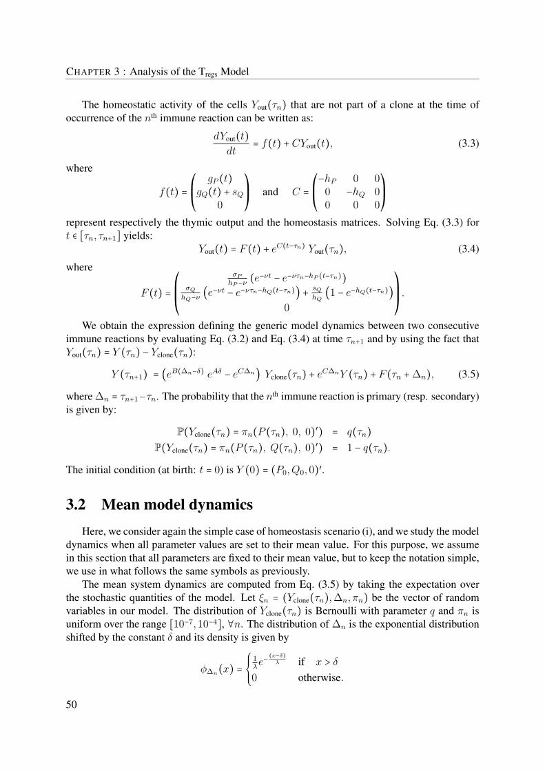
CHAPTER 3 : Analysis of the Tregs Model
The homeostatic activity of the cells Yout(τn) that are not part of a clone at the time ofoccurrence of the nth immune reaction can be written as:
dYout(t)dt
= f(t) +CYout(t), (3.3)
where
f(t) = ⎛⎜⎝gP (t)
gQ(t) + sQ0
⎞⎟⎠ and C = ⎛⎜⎝−hP 0 00 −hQ 00 0 0
⎞⎟⎠represent respectively the thymic output and the homeostasis matrices. Solving Eq. (3.3) fort ∈ [τn, τn+1] yields:
Yout(t) = F (t) + eC(t−τn) Yout(τn), (3.4)
where
F (t) = ⎛⎜⎜⎝σP
hP−ν(e−νt − e−ντn−hP (t−τn))
σQ
hQ−ν(e−νt − e−ντn−hQ(t−τn)) + sQ
hQ(1 − e−hQ(t−τn))
0
⎞⎟⎟⎠ .
We obtain the expression defining the generic model dynamics between two consecutiveimmune reactions by evaluating Eq. (3.2) and Eq. (3.4) at time τn+1 and by using the fact thatYout(τn) = Y (τn) − Yclone(τn):
Y (τn+1) = (eB(Δn−δ) eAδ − eCΔn) Yclone(τn) + eCΔnY (τn) + F (τn +Δn), (3.5)
whereΔn = τn+1−τn. The probability that the nth immune reaction is primary (resp. secondary)is given by:
P(Yclone(τn) = πn(P (τn), 0, 0)′) = q(τn)P(Yclone(τn) = πn(P (τn), Q(τn), 0)′) = 1 − q(τn).
The initial condition (at birth: t = 0) is Y (0) = (P0,Q0,0)′.3.2 Mean model dynamics
Here, we consider again the simple case of homeostasis scenario (i), and we study the modeldynamics when all parameter values are set to their mean value. For this purpose, we assumein this section that all parameters are fixed to their mean value, but to keep the notation simple,we use in what follows the same symbols as previously.
The mean system dynamics are computed from Eq. (3.5) by taking the expectation overthe stochastic quantities of the model. Let ξn = (Yclone(τn),Δn, πn) be the vector of randomvariables in our model. The distribution of Yclone(τn) is Bernoulli with parameter q and πn isuniform over the range [10−7,10−4], ∀n. The distribution of Δn is the exponential distributionshifted by the constant δ and its density is given by
φΔn(x) = ⎧⎪⎪⎨⎪⎪⎩1λe
−(x−δ)
λ if x > δ
0 otherwise.
50

3.3 Model density estimation
We can write:
Eξn[Y (τn+1)] = Eξn [(eB(Δn−δ) eAδ − eCΔn) Yclone(τn)]+ Eξn [eCΔn]Y (τn) +Eξn[F (τn +Δn)]= EΔn [(eB(Δn−δ) eAδ − eCΔn)] EYclone(τn),πn[Yclone(τn)]+ Eξn [eCΔn]Y (τn) +EΔn[F (τn +Δn)],where we have used the fact that Y (τn) is independent of ξn and that Yclone(τn) is independentof Δn. If I is the identity matrix, we have the following results:
EΔn [eB(Δn−δ)] = (I − λB)−1EΔn [eCΔn] = eCδ(I − λC)−1
E[Yclone(τn, πn)] = q(τn) Eπn[πn(P (τn),0,0)′]+(1 − q(τn)) Eπn[πn(P (τn),Q(τn),0)′]= ⎛⎜⎝
π 0 00 (1 − q(τn))π 00 0 0
⎞⎟⎠Y (τn) = U(τn) Y (τn) (3.6)
EΔn[F (τn +Δn)] = λ
⎛⎜⎜⎝σP e−ντn
(1+λν)(1+λhP )σQe−ντn
(1+λν)(1+λhQ)+ sQ
1+λhQ
0
⎞⎟⎟⎠ = F ∗(τn). (3.7)
If we let Y ∗(τn) = Eξn[Y (τn)], we can write
Y ∗(τn+1) = ⎡⎢⎢⎢⎢⎢⎢⎣[(I − λB)−1eAδ − (I − λC)−1eCδ]U(τn)�����������������������������������������������������������������������������������������������������������������������������������������������������������������������������������������������������������������������������������������������������������������������infection matrix: MI
+ (I − λC)−1eCδ�������������������������������������������������������������������������pool-size control: MH
⎤⎥⎥⎥⎥⎥⎥⎦�������������������������������������������������������������������������������������������������������������������������������������������������������������������������������������������������������������������������������������������������������������������������������������������������������������������������������������������������������������������������������������������������������������������������J∗ =MI(τn) +MH
Y ∗(τn) + F ∗(τn)�������������������thymus
= J∗(τn)Y ∗(τn) + F ∗(τn), (3.8)
where U(τn) is given by the square matrix in Eq. (3.6) and F (τn) is given by Eq. (3.7). Themean model dynamics are obtained by applying the iteration of Eq. (3.8) to the initial conditionY ∗(0) = (P0, Q0,0)′, where P0 and Q0 are the average values of P0 and Q0.
3.3 Model density estimation
In order to estimate the model density accurately, we computed confidence intervals on thebivariate histogram depicted in Figure 2.6A of Chapter 2. In this section, we describe how thisis done. This is important because this density is used to formally reject a model scenario.
First, we introduce the necessary theoretical framework. We have a data setX = (x1, . . . , xn)that we view as the realization of a stochastic system (the output of a simulator). We usuallyassume that the model has a density of probability, and that the output (x1, . . . , xn) depends
51

CHAPTER 3 : Analysis of the Tregs Model
on a parameter θ; we denote this density by f(x1, . . . , xn∣θ). It is also called the likelihood ofthe observed data. The framework of parametric estimation theory consists in assuming thatthe parameter θ is fixed, but unknown. An estimator of θ is any function T (⋅) of the observeddata. The maximum likelihood estimator (MLE) is the value of θ that maximizes the likelihoodf(x1, . . . , xn∣θ); we denote it by θ. This definition makes sense if the maximum exists andis unique, which is often true in practice. Definition 1 gives a formal set of conditions thatguarantee the existence and uniqueness of the MLE.
Assume that the parameter θ is multidimensional, i.e., it varies in an open subset Θ of Rk.The observed information is defined by the symmetric matrix
[J(θ)]i,j = −∂2 (θ)∂θi∂θj
,
where (θ) is the log-likelihood defined by
(θ) = log(f(x1, . . . , xn∣θ)).The Fisher information, or expected information is defined by the matrix
[I(θ)]i,j = −Eθ(J(θ)) = −Eθ (∂2 (θ)∂θi∂θj
) ,where the notation Eθ means that the expectation is a function of θ.
Before stating the asymptotic result that leads to the confidence intervals of θ, we state theregularity conditions.
Definition 1. Regularity conditions for maximum likelihood asymptotics.
1. The set Θ of values of θ is compact (closed and bounded) and the true value θ is not onthe boundary.
2. For different values of θ, the densities f(X ∣θ) are different.
3. There exists a neighborhood B of θ∗ and a constant K such that for θ ∈ B and for alli, j, k, n, we have 1
nEθ(∣∂3 X(θ)/∂θi∂θj∂θk∣) ≤ K.
4. For θ ∈ B, the Fisher information has full rank.
5. For θ ∈ B, the interchanges of integration and derivation in∫ ∂f(X ∣θ)∂θi
dx = ∂
∂θi∫ f(X ∣θ)dx
and in ∫ ∂2f(X ∣θ)∂θi∂θj
dx = ∂
∂θi∫ ∂f(X ∣θ)
∂θjdx are valid.
The following theorem is proven in Davison (2003).
Theorem 1. Under the conditions of Definition 1, the MLE θ exists and converges almostsurely to the true value. Further, I(θ)1/2(θ − θ) converges in distribution to a standard normaldistribution, as n goes to infinity. It follows that, asymptotically:
1. the distribution of θ − θ can be approximated by N(0, I(θ)−1) or N(0, J(θ)−1);52

3.3 Model density estimation
2. the ditribution of 2( (θ)− (θ)) (also called the likelihood ratio statistic) can be approx-imated by a chi-square distribution with k degrees of freedom, where k is the dimensionof Θ.
We use the following corollary to define the confidence interval on θ.
Corollary 1. (Asymptotic confidence intervals) When n is large, an approximate confidenceinterval for the ith coordinate of θ is
θi ± η
√[I(θ)−1]i,i
or θi ± η
√[J(θ)−1]i,i, (3.9)
where N0,1(η) = 1+γ2 (for example, with γ = 0.95, η = 1.96).
We apply the above corollary to the estimation of our model’s density. The statistic that weuse is the bivariate histogram of U and V . Remind that U(t) = log(P (t)/(Q(t) +R(t))) andV (t) = log((P (t)+Q(t)+R(t))/T (t)), where T (t) is the total number of T cells at time t. Tosimplify the notation, consider for the moment a univariate histogram, built from n independentobservations that fall into categories 1, . . . , k (the bivariate case is straightforward). Let Yi
denote the number of observations in category i. If πi is the probability that a single observationfalls into category i (0 < πi < 1 and ∑k
i=1 πi = 1), the random variable Y = (Y1, . . . , Yk)′is multinominal with probabilities (π1, . . . , πk) and denominator n. We want to estimate theparameters θ = (π1, . . . , πk)′ of the multinomial. As πk = 1−π1−⋯−πk−1, the parameter spaceis the interior of a simplex in k dimensions, that is, the set
{(π1, . . . , πk) ∶ k∑i=1
πi = 1,0 < π1, . . . , πk < 1}of dimension k − 1. Therefore, there are k − 1 parameters to estimate.
Given data y1, . . . , yk, the likelihood under the multinomial model is
L(θ) = n!
y1!⋯yk!πy11 ×⋯× πyk
k ,k∑i=1
πi = 1, 0 < π1, . . . , πk < 1,
where ∑i yi = n, so the log-likelihood is
(θ) ≃ k−1∑i=1
yi logπi + yk log(1 − π1 −⋯− πk−1).The observed information matrix has general term
− ∂2 (θ)∂πi∂πj
= ⎧⎪⎪⎨⎪⎪⎩yiπ2i+ yk
(1−π1−⋯−πk−1)2, for i = j
yk(1−π1−⋯−πk−1)2
for , i ≠ j,,
where i and j run over 1, . . . , k−1. It is easy to see that the maximum likelihood estimators areπi = Yi/n. The expected information matrix involves E(Yi), which is calculated by noting that
53

CHAPTER 3 : Analysis of the Tregs Model
the marginal distribution of Yi is binomial with probability πi and denominator n. The mean ofYi is therefore nπi. Thus, the expected information matrix is:
I(θ) = n
⎛⎜⎜⎜⎝1/π1 + 1/πk 1/πk ⋯ 1/πk
1/πk 1/π2 + 1/πk ⋯ 1/πk⋮ ⋮ ⋱ ⋮1/πk 1/πk ⋯ 1/πk−1 + 1/πk
⎞⎟⎟⎟⎠whose inverse is:
I(θ)−1 = 1
n
⎛⎜⎜⎜⎝π1(1 − π1) −π1π2 ⋯ −π1πk−1−π2π1 π2(1 − π2) ⋯ −π2πk−1⋮ ⋮ ⋱ ⋮−πk−1π1 −πk−1π2 ⋯ πk−1(1 − πk−1)
⎞⎟⎟⎟⎠ . (3.10)
Provided that none of the πi equals zero or one, the regularity conditions of Definition 1 holdand Theorem 1 applies with I(θ)−1 given by Eq. (3.10), giving us the confidence interval of πi:
πi ± η
√(1nπi(1 − πi)), (3.11)
where N0,1(η) = 1+γ2 .
54

Part II
Measuring T-cell Receptor Diversity


Chapter 4Mathematical Modeling of AmpliCot
4.1 Introduction
The diversity of T cell receptors (TCRs) is part of the polymorphism of our adaptive im-mune system and is responsible for the recognition and the defense against possibly an universeof different pathogens. The structural diversity of TCRs is achieved by somatic gene-segmentrearrangements and random nucleotide additions or deletions (Goldsby et al., 2003). The es-timation of the effective size of the human TCR repertoire, both in health and disease, is afundamental question in immunology and yet, not fully addressed.
A common way to tackle this problem consists in the following two steps: (1) samplingthe repertoire of an individual to measure the sample diversity; (2) extrapolating the wholerepertoire diversity from the sample diversity. The first step of this “general approach" is oftenrather experimental, whereas the second is rather theoretical, as discussed in Section 4.1.1.The work presented in this chapter concerns the first step above and combines experiments andmathematical modeling in order to better estimate the diversity of a sample.
Several experimental techniques aim at the measurement of the structural TCR diversityof a repertoire sample. Immunoscope (or Spectratype) gives a qualitative insight of the reper-toire’s shape in terms clonal sizes (Currier and Robinson, 2001; Pannetier et al., 1993); high-throughput DNA sequencing exhaustively enumerates the clonotypes of a sample, thus provid-ing a more detailed picture of the repertoire (Mardis, 2008; Shendure and Ji, 2008). AmpliCotis an alternative experimental technique that allows the sample diversity measurement throughquantitation of the re-hybridization speed of denatured PCR products (Baum and McCune,2006). This elegant approach has the advantage over the cloning and sequencing methods tobe time- and expense- effective. However, in order to obtain accurate diversity estimates, theassay should be performed under very stringent experimental conditions.
The AmpliCot experiment is based on the so-called “Cot analysis" (Britten and Kohne,1968), according to which the time required for a DNA sample to reanneal (expressed in termsof the product nucleotide concentration × time, “Cot") is related to the diversity of the sample.In short, fluorescent SYBR green dye, which binds double-stranded DNA, is added to a sampleof PCR-amplified cDNA. The sample is melted, such that the DNA becomes single-stranded,and reannealed under very strict conditions in order to avoid heteroduplex formation and allow
57

CHAPTER 4 : Mathematical Modeling of AmpliCot
only for the association of perfectly complementary strands (homoduplexes). 1 The annealingkinetics, measured in terms of fluorescence intensity, are a function of the diversity and of theconcentration of the sample, and have been interpreted assuming second order kinetics.
In order to read the diversity from the resulting annealing curve, Baum and McCune (2006)propose a simple method. It consists in considering the Cot value at which 50% of the sampleis annealed (Cot1/2 value) as a function of diversity. The authors suggest that the relation be-tween these quantities is linear. This statement presumes the validity of second order kinetics(SOK) as a correct model for the annealing kinetics (Yguerabide and Ceballos, 1995). Accord-ingly, only perfectly complementary pairs of DNA can associate, precluding the possibilityof heteroduplex formation. Under the “stringent" conditions defined in Baum and McCune(2006), SOK would indeed hold. However, it is possible that a slight deviation from the “ideal"experimental settings leads to some heteroduplex formation, which would bias the diversityestimation.
We therefore have two motivations to define a mathematical model of AmpliCot. First,driven by the fact that SOK might be an over-simplified model, we define a more detailedscheme in which the formation of transient complexes and heterdoduplexes is allowed. Second,we consider that sampling the annealing curve at a single point (the Cot1/2 value) is not takingadvantage of all the available information in the data. We believe that the diversity extrapolationmethod can be improved by using the information contained in the entire annealing curve.
Thus, in this chapter, we define a mathematical model that describes the annealing kineticsof AmpliCot and use it to propose an alternative diversity extrapolation procedure. To fit themodel parameters and to test our diversity predictions, we use “toy" data sets consisting intemplates of known diversity from a library of individually synthesized oligonucleotides.
4.1.1 TCR repertoire assessment: State of the art
In this section, we give a (non-exhaustive) overview of the recent advances in the TCRrepertoire assessment. In particular, we focus on studies using mathematical modeling or ad-vanced statistical analysis. Although the experimental settings evoked here can be used tomeasure the structural diversity of BCRs and antibodies, we consider only examples in whichthey have been used to study TCRs. In addition, a large part of the existing diversity assess-ment literature concerns the repertoire of αβ T cells. Therefore, unless explicitly stated, TCRdiversity refers in this section to the structural diversity of αβ TCRs.
The main difficulty in the estimation of TCR diversity comes from the fact that the latterhas to be extrapolated from samples containing only a small part of the entire repertoire. Thedifficulty is further increased by the unknown shape of the clonal sizes distribution. A lowerbound estimate was obtained by assuming that all clonotypes are equally represented, as inArstila et al. (1999). Using TCR gene amplification and sequencing, the authors found thatthere are about 106 different β chains in human blood and that each of these chains can bind,on average, to at least 25 different α chains. Therefore, a lower bound on the human TCRdiversity was set to 2.5×10⁷. A similar approach was used in Casrouge et al. (2000) to estimate
1. In the context of this chapter, a heteroduplex is a double-stranded DNA (dsDNA) molecule composed oftwo imperfectly matching single strands. A homoduplex is a dsDNA molecule with perfectly matching strands.
58

4.1 Introduction
the size of the TCR repertoire of naive mouse splenocytes. In these early studies, the use ofmathematics was rather limited and modeling was not involved.
From a theoretical point of view, De Boer and Perelson (1993) developed a probability-based model in order to answer the question “How diverse should the immune system be?"Interestingly, the authors find that it is not the large number of foreign antigens that induces anenormous repertoire diversity, but rather the number of self antigens the immune system needsto avoid reactivity with. Later, Borghans et al. (1999) adopt a similar methodology to addressthe specificity of immunological memory. One of the conclusions of the authors is that memorylymphocytes should be more specific than the naive ones.
In the last decade, important advances in terms of experimental techniques have beenachieved and with them, statistical and computational methods specifically applied to thesetechniques have started developing. Hitherto, the main data source seems to be the so-calledhigh-throughput DNA sequencing (Mardis, 2008; Shendure and Ji, 2008). The latter is anoptimized and more efficient version of the capillary-based sequencing used in the above-mentioned early studies (Arstila et al., 1999; Casrouge et al., 2000). T cells are sampled fromthe blood and are possibly sorted according to a surface receptor in order to isolate functionalsubsets, such as naive or memory cells (Wang et al., 2010). The DNA (or mRNA) coding forthe complementarity determining region 3 (CDR3) of the TCR is then amplified and sequenced.The resulting data set contains the number of different DNA sequences and their frequency inthe sample, i.e., all the information about the sample distribution. It is therefore straightfor-ward to put the information in the desired form and, for example, estimate the clonotype or theclonal size distribution. An example of data representation can be found in Robins et al. (2009,Fig.6B), where the authors display a histogram of CDR3 sequences with certain length that usea certain gene segment. The availability of such detailed data sets made urgent the developmentof statistical estimators of the whole-repertoire diversity.
Estimating the diversity of TCRs is in fact a particular instance of a classical problem instatistics. The general setting is that of a population (TCRs) partitioned into a number of classes(clonotypes), each class corresponding to a distinct species. The goal is to estimate the numberof different classes. Applications of that problem are found in numerous fields: in ecology forestimating the biodiversity of plants or animals, in computer sciences for database or socialnetwork searches, in linguistics for estimating the size of an author’s vocabulary (Efron andThisted, 1976), and many others. Theoretically, there are several ways to tackle the problem,according to whether the population size is finite or infinite (see Bunge and Fitzpatrick (1993)for a review). In the context of TCR diversity estimation, the most common approach is toconsider the “species sampling" process. The latter can be viewed as a stochastic process wherenew species “arrive" in a sample according to a Poisson process with a rate, itself varyingaccording to a parametric (mixing) distribution. This approach (or other approximations ofit) has been recently adopted by numerous groups (Rempala et al., 2010; Robins et al., 2009;Sepúlveda et al., 2010). Although the full TCR repertoire assessment remains an open question,using the above-mentioned statistical tools has led to refined diversity estimations. The latest ofthese (Robins et al., 2009) evokes a TCRβ receptor diversity at least 4-fold higher than previousestimates and 10-fold higher in the subset of antigen-experienced T cells.
Data output from other experimental techniques aiming the diversity assessment appear inother forms. For example, Immunoscope/Spectratype produces a histogram of CDR3 lengths,
59
CHAPTER 4 : Mathematical Modeling of AmpliCot
but gives no information about the diversity or the clonal size distribution. In AmpliCot, thedistributional information is inherent to the data, but not directly available. Expanded clonesare therefore more difficult to detect. This is why an additional modeling step is necessary toaccess all the information contained in the experimental data before extrapolating the wholerepertoire diversity from a data sample.
4.1.2 Our Contributions
As mentioned earlier, the work presented here aims at the correct diversity estimation ofa given repertoire sample. In the literature overviewed in the previous section, most of thetheoretical and computational efforts focused on addressing the second step of the “general ap-proach", namely inferring the whole-repertoire diversity from the measured sample diversity.The measurement technique was mainly DNA sequencing. Alternatives to high-throughput se-quencing, such as AmpliCot, have not been widely used, partly due to the lack of methods fordata analysis or to other experimental issues (Schütze et al., 2010). The main contribution ofthis chapter is the improvement of the interpretation of AmpliCot’s experimental data. To ourknowledge, this is the first time that a mathematical model is used to describe this particular ex-perimental technique. As a result to our modeling, we show that the underlying model assumedin the original paper by (Baum and McCune, 2006) is insufficient to explain AmpliCot experi-mental data. A more detailed model, assuming heteroduplex- and transient duplexes formation,leads to significantly better data fits and accounts for the fluorescence loss observed in (Schützeet al., 2010). As a consequence, we show that the Cot-based method for interpreting the resultsof AmpliCot suggested in (Baum and McCune, 2006) should be applied with caution. Finally,we suggest alternative methods for sample diversity extrapolation.
4.1.3 Chapter Outline
This chapter is organized as follows. In the next section, among other methodological de-tails, are presented the AmpliCot assay (Section 4.2.1), the DNA annealing kinetics models(Section 4.2.3) and the diversity extrapolation methods (Section 4.2.10). The results (Sec-tion 4.3) are then followed by a discussion (Section 4.4).
60

4.2 Materials and Methods
4.2 Materials and Methods
4.2.1 AmpliCot Assay
Samples containing PCR-amplified TCR genes of lymphocytes (or artificially synthesizedoligonucleotides) were mixed with SYBR green fluorescent dye, which binds to double-strandedDNA. Aliquots of this mixture were placed in the upper and lower rows of a 96-well plate asthe annealing sample and the reference (Figure 4.1A). A replicate (if any) was placed one rowbelow the original sample. The pre-anneal step consists of measuring the baseline fluorescenceof the samples and of the reference at annealing temperature (Figure 4.1B). Then, the temper-ature is increased for 2 minutes and the samples melt, whereas the reference stays at annealingtemperature (melting step). Note that there is approximately a one-degree difference in thetemperatures at which two replicates are melted, caused by the temperature gradient featureof PCR machines. The fluorescence intensity of the samples is strongly decreased during themelting step, as double-stranded DNA de-hybridizes. During the annealing step, the tempera-ture of the samples was set back to annealing temperature and the fluorescence intensity as afunction of time was measured every 5-20 seconds (Figure 4.1B). At equal concentrations, there-annealing rate is dependent on the diversity of the sample.
4.2.2 Experimental data
Templates of known diversity were created from a library of individually synthesized oligonu-cleotides and are composed of 64 base pairs, out of which a maximum of 16 can differ. Ampli-Cot was performed on samples where all sequences are present in equimolar ratio. We had atour disposal three data sets: the original oligonucleotide data set of Baum & McCune (Baumand McCune, 2006, Fig.2a) and two other data sets obtained at the University Medical CenterUtrecht (UMCU). To slow down the annealing kinetics, low diversity samples of UMCU dataset 1 were diluted. The inverse of the dilution factor was used as a sample’s concentration.For the other two data sets, the dilution (and therefore the concentration) was the same for alldiversities. Table 4.1 summarizes the three data sets.
Data set Diversities Nb. of replicates Dilution factor
Baum &McCune
n = 1,2,5,10,30,48,96 1 Same for all n
UMCU1n =1,4,8,16,32,48
2 (n = 1,4,8,16) 1:4 (n = 1,4)1 (n = 32,48) 1:2 (n = 8,16,32,48)
UMCU2 n = 10,20,30,40 2 Same for all n
Table 4.1: The three data sets of known diversity templates at our disposal.
61

CHAPTER 4 : Mathematical Modeling of AmpliCot
4.2.3 Modeling the DNA Annealing Kinetics
Second Order Kinetics (SOK)
Second order kinetics is the minimal model that describes the annealing phase of AmpliCot.It expresses the fact that two complementary single strands of DNA anneal and form a homo-duplex. Consider a DNA sample of diversity n. Let Si be the concentration of single-strandedDNA (ssDNA) molecules of type i, and Dii be the concentration of homoduplexes of type i,i = 1, . . . , n. We call a the rate of association of two single-stranded molecules. Assuminga well mixed solution and a large number of molecules, the following differential equationsdescribe the second order kinetics model (Figure 4.1C):
dSi
dt= −2aS2
i
dDii
dt= aS2
i . (4.1)
Let t0 = 0 be the beginning of the annealing phase of AmpliCot and let T be the total concen-tration of ssDNA molecules inside a sample. Let fi be the proportion of ssDNA of species i atthe beginning of the annealing phase. Assuming that there is no loss of matter, if all dsDNA isdenatured after the melting phase of AmpliCot, there would be fiT single-stranded moleculesof type i at the beginning of the annealing phase and no dsDNA. However, as the fluorescencelevel at melting temperature is not exactly 0, some molecules are possibly in double-strandedform. We call α the proportion of melted molecules at t0 (α ∈ [0,1]). The initial conditions arethus Si(0) = αfiT and 2Dii(0) = (1 − α)fiT , i = 1, . . . , n. Let F (t) be the concentration offluorescent molecules at time t. In the case of second order kinetics,
F (t) = 2n∑i=1
Dii(t) = T − n∑i=1
Si(t).
Complete Model (CM)
This model describes in further detail the biochemical reaction of AmpliCot. We considerthe fact that the hybridization involves two steps and it might result in heteroduplex formationbecause of erroneous associations (Figure 4.1C). Encounters of two single DNA strands oc-cur at rate a. Two strands form either a partially hybridized homoduplex Cii if they are bothperfectly complementary, or a partially hybridized heteroduplex Cij otherwise. Partially hy-bridized homoduplexes (resp. heteroduplexes) can dissociate at rate d1 (resp. d2), or hybridizecompletely at rate z1 (resp. z2) to form the final product Dii (resp. Dij). The differential
62

4.2 Materials and Methods
equations describing the change in time of the above-mentioned concentrations are:
dSi
dt= −2aS2
i − aSi
n∑j=i+1
Sj + 2d1Cii + d2n∑
j=i+1
Cij
dCii
dt= aS2
i − (d1 + z1)Cii
dCij
dt= aSiSj − (d2 + z2)Cij (4.2)
dDii
dt= z1Cii
dDij
dt= z2Cij,
where i = 1, . . . , n and j = i+1, . . . , n. We assume that that the melting process is fast comparedto the re-annealing, and that the melting temperature is so high that no re-hybridization is oc-curring during the melting phase. Under these hypotheses, the sample contains only ssDNA orunmelted dsDNA homoduplexes at the beginning of the annealing phase. The initial conditionsfor the above system are thus Si(0) = αfiT ,Dii(0) = (1−α)fiT , Cii(0) = Cij(0) = Dij(0) = 0,i = 1, . . . , n, j = i+1, . . . , n, α ∈ [0,1]. We assume that heteroduplexes have a decreased fluores-cence intensity compared to homoduplexes and we model this by weighting their fluorescenceby a factor ϕ ∈ [0,1]. The concentration of fluorescent molecules is therefore defined as
F (t) = 2( n∑i=1
Dii(t) +ϕn∑i=1
n∑j=i+1
Dij(t)) .4.2.4 Mean Field Models
An analytic solution for second order kinetics is easy to find, but this is not the case forthe complete model. Solving numerically the above differential equations is computationallyexpensive because the size of the system grows with the diversity n. However, when the DNAparticles of each species are in equimolar concentrations in the annealing buffer, the abovedifferential equations can be simplified by using the fact that if fi = 1/n, the dynamics of thewhole system are proportional to the dynamics of the individual species. In other words, thedynamics of one specie are equal to the mean of all species. Using this property allows areduction of the number of variables from O(n) (in the case of second order kinetics) or O(n2)(in the case of the complete model) to O(1) (2 or 5 variables). This simplification is thusremoving the dependence of the system size on the diversity. Hence, solving the differentialequations numerically is no longer a hurdle because the computational cost of the numericsolution is constant. This is very important when dealing with samples of diversity in theorders of millions, such as, for example, DNA from human naive T cells. The derivation of themean field equations are given in the following two sections.
Mean Field Second Order Kinetics
Let S(t) = ∑ni=1 Si(t) andD(t) = ∑n
i=1Dii(t). If all species are in equimolar concentrationsin the mixture, we have Si(t) = Sj(t), i ≠ j, ∀t. Therefore, S(t) = nS1(t), D(t) = nD11(t)
63

CHAPTER 4 : Mathematical Modeling of AmpliCot
and the differential equations Eq. (4.1) become
dS
dt= −2aS2
n(4.3)
dD
dt= a
S2
n,
where we have used the fact that nS21 = S2/n. The solution of this system with initial conditions
S(0) = αT and 2D(0) = (1 − α)T is:
S(t) = αT
1 + 2 anαTt
2D(t) = T − S(t),and the fluorescent molecules
F (t) = 2D(t). (4.4)
Mean Field Complete Model
Assuming equimolar concentrations of each species, we define the following quantities:
S(t) = n∑i=1
Si(t) = nS1(t)C(t) = n∑
i=1
Cii(t) = nC11(t)H(t) = n∑
i=1
n∑j=i+1
Cij(t) = n(n − 1)2
C12(t) (4.5)
J(t) = n∑i=1
n∑j=i+1
Dij(t) = n(n − 1)2
D12(t)D(t) = n∑
i=1
Dii(t) = nD11(t),where indices 1 and 2 have been chosen arbitrarily to design one species. S(t) denotes ssDNA,C(t), partially hybridized homoduplexes, H(t), partially hybridized heteroduplexes, J(t), fi-nal product heteroduplexes and D(t), the final homoduplexes. The differential equations ofEq. (4.2) can be written in terms of the above variables as follows:
dS
dt= −a(n + 1)S2
n+ 2d1C + 2d2H
dC
dt= a
S2
n− (d1 + z1)C
dH
dt= a(n − 1
2) S2
n− (d2 + z2)H (4.6)
dJ
dt= z2H
dD
dt= z1C,
64

4.2 Materials and Methods
with initial conditions S(0) = αT , 2D(0) = (1−α)T , C(0) = H(0) = J(0) = 0, and fluorescentmolecules
F (t) = 2(D(t) +ϕJ(t)). (4.7)
This system of differential equations is solved numerically.
4.2.5 Modeling the AmpliCot Assay
Let R(t) and Araw(t) be respectively the fluorescence intensity of the reference and of thesample at time t (in minutes). Let tm be the start of the melting step and t0 > tm be the start ofthe annealing step (Figure 4.1B). We adopt the following convention: t0 = 0, which implies thattm < 0. Let Ab be the baseline fluorescence of the sample, which we define as the fluorescenceintensity at time 0 (Figure 4.1B). Similarly, let Rb be the baseline fluorescence of the reference.The following equations describe the pre-annealing and the annealing step of AmpliCot (we donot model the melting step, as it does not contain any pertinent information about diversity):
R(t) = Rbh(t) (4.8)
Araw(t) = ⎧⎪⎪⎨⎪⎪⎩Abh(t) for t < tm
AbF (t;Θ, α)h(t) for t ≥ t0,(4.9)
where F (t;Θ, α) ∈ [1 − α,1] is the concentration of fluorescent molecules determined by thebiochemical reaction model (SOK (Eq. (4.4)), or CM (Eq. (4.7))), with reaction rates Θ, totalconcentration T = 1 and proportion α of melted molecules at time 0. The function h(t) de-scribes phenomenologically the slow fluorescence decay due to degradation of the SYBR greendie (Baum and McCune, 2006). It has the following expression:
h(t) = (K1e−δ1t +K2e
−δ2t + (1 −K1 −K2)) , (4.10)
where K1,K2 ∈ [0,1] and δ1, δ2 > 0.
4.2.6 Model Fitting to Experimental Data
In order to determine which of the above models of DNA annealing kinetics describes theexperimental data best, we fitted each model to the three data sets. The mean field versions ofthe differential equations were solved numerically (except for the second order kinetics model,where an analytical solution is available) using a Runge-Kutta algorithm written in C. Theparameters were fitted using a least squares procedure (implemented in Matlab) applied to thelog-transformed raw annealing curves.
We assume that some parameters are common to all samples on the samples plate, whereasothers are specific to each sample. We therefore splited the parameters in two groups: thecommon parameters Θ, and the sample-specific parameters Ω. The biochemical reaction ratesand the fluorescence of heteroduplexes are common to all samples, whereas the fluorescencedecay parameters (Eq. (4.10)) and the baseline fluorescence are specific to each sample. Theproportion α of DNA molecules that are in single-stranded form at the beginning of the an-nealing phase is assumed to be common to all samples placed on the same row of the plate.
65
CHAPTER 4 : Mathematical Modeling of AmpliCot
The replicates (if any) placed on another row were allowed to have a different α value, becausethe temperature at which samples are melted varies from one row to another 2 and thereforethe amount of melted material observed after the same melting period can be slightly differ-ent. To simplify notations, we consider α as a common parameter and we make the distinctionwhenever unclear. To summarize, we have
Θ = (a, d1, d2, z1, z2, ϕ,αj) (4.11)
Ωi = (δ(i)1 , δ(i)2 ,K
(i)1 ,K
(i)2 ,R
(i)b ,A
(i)b ), (4.12)
where i denotes the ith sample in a given experiment, i = 1, . . . ,N , and j denotes the replicateindex (if any), j = 1 or 2. The reference of each sample is used to fit δ1, δ2, K1, K2 and Rb.Note that if the pre-anneal measurements are long enough, they can be used as an alternativeto fit the fluorescence decline parameters. The baseline fluorescence intensity of the sample(Ab) was estimated using the last 10 measurements of the pre-anneal step and corrected for thefluorescence decline during the melting step obtained from the reference. The annealing curvesof all diversities were used to fit the common reaction rates Θ (Eq. (4.11)).
To slow down the annealing kinetics of samples with low diversities, some samples werediluted (cf. Table 4.1). The inverse of the dilution factor was used as an indicator of theconcentration. Theorem 2 in Chapter 5 shows how dilution of a sample affects the reactionrates.
4.2.7 Confidence Intervals on Parameter Values
The 95% confidence intervals on parameter values were computed using 999 bootstrapreplicates of each original data set. The bootstrap was done by sampling with replacement pairsof points (ti,Araw(ti)) from pre-anneal and annealing curves. The bootstrap replicates wherefitted in the same way as the original data set (see Section 4.2.6). To avoid that the optimizationprocedure gets trapped in the same local minimum when applied to bootstrap replicates, theinitial point of the fitting procedure was randomized. The confidence intervals are computedusing order statistics of the bootstrap distribution (Le Boudec, 2010).
4.2.8 Computing the Annealing Percentage (or Data Normalization)
In order to compute the percentage of annealed material, the raw sample was normalized.This was done by correcting for the baseline fluorescence discrepancies of the reference andthe sample and by correcting for the time-dependent fluorescence decline. In addition, in orderto obtain a percentage of annealed material in the range 0–1, the fluorescence of the sample atmelting temperature (rescaled to the reference baseline, i.e., α in the notation of the model) wassubtracted from the corrected annealing curve. Note that the latter transformation is only validunder the assumption that the fluorescence at melting temperature is due to measurement noiseand is not an indication of annealed material. Let A(t) be the resulting normalized annealing
2. There is approximately one-degree difference in the in the temperatures at which two replicates are melted,caused by the temperature gradient feature of PCR machines.
66
4.2 Materials and Methods
curve expressed in "percentage annealed". We obtain A(t) from the raw data for t ≥ t0 byapplying the above transformations:
A(t) = Araw(t)R(t) − Am
Rb
Ab
Rb− Am
Rb
= Rb
Ab −Am
(Araw(t)R(t) − Am
Rb
) . (4.13)
The above equation was used to normalize the data, where Ab and Rb were estimated by themean of the last 10 measurements of the pre-anneal phase and Am was estimated by the meanof the measurements during the melting step. If these measurements were not available, Am
was set to the first measurement of the annealing step. According to Baum andMcCune (2006),the normalized data should be considered in concentration × time (Cot) units to account for theeffect of the concentration differences in the annealing speed of samples. We have used theinverse of the dilution factor (whenever known) as an indicator of the concentration.
If the model is fitted on the raw data and then needs to be transformed in normalized form,the above equation can be further developed and simplified in order to be expressed in terms ofthe model parameters. Indeed, the fluorescence Am of the sample after the melting reflects theconcentration of unmelted material, which is expressed as F (0) = 2(D(0)+ϕJ(0)) = 2D(0) =(1 − α)T . A fluorescence intensity of Ab is associated to the total concentration T , thereforethe fluorescence at melting temperature can be written as Am = f(F (0)) = (1 − α)Ab. Thus,following the definition of Araw(t) (Eq. (4.9)) and of R(t) (Eq. (4.8)), one can write:
A(t) = Rb
Ab −Am
(AbF (t;Θ, α)h(t)Rbh(t) − Am
Rb
) (4.14)
= 1
αAb
(AbF (t;Θ, α) − (1 − α)Ab))= 1
α(F (t;Θ, α) − (1 − α))
Th.1= F (t;αθ1, θ2,1),where the last equality holds following Theorem 2 of the Appendix. F (t) is defined in Eq. (4.4)or Eq. (4.7), depending on the model.
4.2.9 Cotp and tp Values Estimation
In the original AmpliCot paper (Baum and McCune, 2006), to correct for concentrationdifferences, time is multiplied by the nucleotide concentration of a sample (Cot = Concentration× time). From the normalized data, one can estimate the Cot value at which a proportion p ofthe sample has annealed (p ∈ [0,1]). This is what we call a Cotp value (equivalently, a "CotX%" value). A tp value is simply the time at which a proportion p of the sample has annealed(p ∈ [0,1).
To estimate a tp value from noisy data, we defined a precision interval around p, say [p −ε/2, p + ε/2], where ε is the precision level. We considered the data points that fall inside theabove interval. Let t be the set of time coordinates of these points. As the annealing curve ismonotonous and the measurement error small, it can be assumed that the search tp value, say
67
CHAPTER 4 : Mathematical Modeling of AmpliCot
t∗p , is in t. If ε is small enough, the annealing curve is locally approximately linear. Therefore,taking simply t∗p ≈ (min(t) + max(t))/2 is approximately correct. Of course, this simpleapproximation is sensitive to aberrant values, but since the data is rather smooth and does notpresent big deviations from its mean value, this approximation should yield correct results. Thesame procedure was applied to Cotp values.
4.2.10 Diversity Prediction Methods
A diversity prediction consists of analysis of samples of oligonucleotides with known di-versity as a training set for calibration, then predicting the diversity of a sample with unknowndiversity. We consider three different methods of prediction. The first method is the one sug-gested in Baum and McCune (2006), which we call the “Cot-based" prediction method. Inshort, the normalized annealing curves are considered at a single point (the Cot point at whichX% of the material has annealed) and one assumes a linear relation between Cot X% and di-versity n (Eq. (4.15)), as predicted by second order kinetics. The slope of the latter relationis estimated using a linear regression and the unknown diversity is predicted from the inverserelation evaluated at the Cot X% point of the unknown sample.
We propose two alternative methods. The "model-based" method intends to use not onlythe information of the annealing curves sampled at one point as in the previous procedure, butthe information contained in the entire annealing curve. It also has the advantage of having thechoice of using the raw or the normalized data. The "model-based" prediction uses the samplesof known diversity to fit the parameters of the underlying annealing kinetics model (secondorder kinetics or the complete model). The biochemical reaction rates are then fixed to theirbest-fit values and a range of possible values of the diversity n is determined. For each valueof this pre-determined set, the remaining parameters are estimated by fitting the model to thesample with unknown diversity by minimizing the least-squared errors of the log-transformeddata and model. The log-likelihood of the resulting fit is calculated. The unknown diversity isestimated as the value of n that maximizes the log-likelihood.
The third method, called "tp-based", is an improved version of the above Cot-based method.It uses tp values, but instead of assuming a linear relation between tp and n, it uses the best-fitof the model to infer the (possibly nonlinear) relation. The unknown diversity is read from theinverse relation. Table 4.2 summarizes the three prediction methods.
Note that the Cot-based method is assuming second order kinetics as the underlying modelfor the annealing kinetics. The other two methods can be applied assuming one or the otherunderlying models, i.e., second order kinetics or the complete model. However, for the rest ofthe manuscript, we will apply both the model- and the tp-based methods assuming the completemodel.
4.2.11 Confidence Intervals on Predictions
In order to test the accuracy of the above prediction methods, we used the low diversitysamples to execute the calibration step of the procedures and we predicted one of the highdiversity samples (n = 48 or 96, depending on the data set). A confidence interval on theprediction was computed by bootstrapping the diversities on which the model was calibrated
68

4.2 Materials and Methods
Method Calibration Prediction
Cot-based 1. Normalize the data. 1. Estimate the Cotp of the un-known diversity sample.
2. Choose a value of p ∈ [0,1]. 2. Return the value n∗ atwhich the linearregression is equal to theestimated Cot.
3. Estimate Cotp values for eachknown diversity.4. Do a linear regression on theCotp values as function of n.
Model-
based
1. Fit the common parameters Θ(Eq. (4.11)) of the model (sec-ond order kinetics or the com-plete model) to the raw data ofthe known diversity samples.
1. Given a value of n ∈N and the best-fitting com-mon parameters Θ (Eq. (4.11)),fit the remaining parameters Ω(Eq. (4.12)) to the raw data of theunknown diversity sample andcompute the likelihood of the re-sulting fit.
2. Define a large set N of pos-sible diversities susceptible tocontain the unknown diversity.
2. Repeat step 1. for all n ∈ N .
3. Return the diversity n∗ withthe highest likelihood.
tp-based 1. Fit the common parameters Θ(Eq. (4.11)) of the model (sec-ond order kinetics or the com-plete model) to the raw or nor-malized known diversity sam-ples.
1. Estimate the value tp ofthe unknown diversity sample bynormalizing it.
2. Normalize the data and themodel (if not fitted on normal-ized data).
2. Return the value n∗ at whichthe (nonlinear) inferred tp(n) re-lation is equal to tp.
3. Choose a value of p ∈ [0,1].4. Based on the best-fit param-eters, infer the relation tp(n) forlarge n.
Table 4.2: Prediction methods. The Cot-based method is the one suggested in (Baum andMcCune, 2006) and is based on the assumption that second order kinetics is the correct under-lying model to describe AmpliCot experiments. The Model-based method uses any underlyingmodel that is fitted to the full data set; the best-fit parameters are then used to extrapolate anunknown diversity using the entire annealing curve (not only sampled at one point as in theCot-based method). The tp-based method is a hybrid of the other two: it considers Cot values,but does not assume a linear relation between Cot and n.
69

CHAPTER 4 : Mathematical Modeling of AmpliCot
(at least 500 bootstrap replicates). The diversity of the unknown sample was estimated for eachset of bootstrapped calibration curves and statistics were performed on the resulting bootstrapprediction distribution.
70
4.3 Results
4.3 Results
4.3.1 Two Models Describing AmpliCot
The aim of AmpliCot is to measure the diversity of a pool of DNA sequences and hasbeen applied to measure TCR diversity (Baum and McCune, 2006). Samples containing PCR-amplified products (be it from TCR or BCR genes of lymphocytes or artificially synthesizedoligonucleotides) are mixed with SYBR green fluorescent dye, which binds double-strandedDNA (dsDNA). Aliquots of this mixture are placed in the upper and lower rows of a 96-wellplate as the annealing sample and the reference (Figure 4.1A). A replicate (if any) is placed onerow below the original sample. The AmpliCot procedure is comprised of three steps: the pre-anneal, melting and annealing step (Figure 4.1B). The pre-anneal step is intended to measurethe baseline fluorescence of samples and references at annealing temperature. Preliminaryexperiments are performed in order to determine the optimal annealing temperature. In manycases, it is set to three degrees less than the melting temperature Tm. During the melting step,the temperature is increased to Tm for two minutes, which leads to the dissociation of dsDNA.By breaking its hydrogen bonds, dsDNA falls apart into two single-stranded DNA molecules.As a consequence, the fluorescence intensity of the sample strongly decreases. During theannealing step, samples are put back at annealing temperature and their fluorescence slowlyincreases as ssDNA molecules re-associate. Fluorescence readings are performed every 5–20 seconds, depending on the experiment. At equal concentrations, the re-annealing rate isdependent on the diversity of the sample.
We consider two models describing the biochemical reaction of the annealing step of Am-pliCot: second order kinetics (SOK) and the complete model (CM) (Figure 4.1C). We assumethat samples contain a large amount of DNA and that the material is well-mixed, so both mod-els are defined using ordinary differential equations. The main difference between the modelsis the level of detail incorporated in the description of the underlying biochemical reaction.
Second order kinetics is the simplest model that allows the description of AmpliCot. It re-lates the association of two perfectly complementary single DNA strands under the assumptionthat the encounter of two strands is the rate limiting step and that the subsequent polymeriza-tion is fast compared to the former process. Under these assumptions, the hybridization of DNAis indeed a second order reaction. The differential equations describing SOK can be found inEq. (4.1). This model was proposed in the original AmpliCot paper (Baum andMcCune, 2006).
The complete model takes into account the fact that hybridization involves two distinctprocesses: the association of short, homologous sites on two single strands, followed by a re-versible polymerization (Wetmur and Davidson, 1968). The partially associated complexes caneither fall apart or definitely associate. The model also accounts for the possibility of heterodu-plex formation which happens in two steps, similarly to homoduplex formation. A detaileddescription of the complete model and the differential equations describing it (Eq. (4.2)) can befound in the Materials and Methods (Section 4.2.3).
71

CHAPTER 4 : Mathematical Modeling of AmpliCot
A BSampleReplicate
Reference
C
Fluo
resc
ence
inte
nsity R(t)
Reference
Sample
Tem
pera
ture
A (t)raw
A
R
t0mt
b
b
Pre−anneal Annealing step
Time
Melting step
95°C
Figure 4.1: The AmpliCot assay and model. A: Samples containing PCR-amplified TCR genesor oligonucleotides are placed on both extremities of a 96-well plate as the samples and thereference. B: Data collection in a real-time PCR machine. The baseline fluorescence intensityof samples and reference is measured at annealing temperature (pre-anneal step). The sampleis then melted at 95○C and its fluorescence drops (melting step). After 2 min. of melting, thetemperature of the sample is quickly set back to annealing temperature to allow for re-annealingof DNA strands (annealing step). C: Two possible models of the biochemical reactions occur-ring during the annealing step of AmpliCot. Second order kinetics (top line) is the minimalmodel in which only homoduplexes are formed. The complete model (bottom line) considersthe reaction in more details. The association occurs in two steps, a first encounter, followed bya zippering reaction. It also includes the possibility of heteroduplex formation.
4.3.2 The SOK model gives a good description of Baum&McCune’s data
In order to evaluate which model best reflects the experimental reality, we have fitted bothmodels to the raw data of Baum and McCune (2006). For details on the fitting procedure, werefer the reader to Section 4.2.6 of the Materials and Methods.
Figure 4.2 illustrates the experimental data of the pre-anneal (t < 0) and the anneal (t ≥ 0)steps of AmpliCot, together with the best-fit of both models (green: SOK, red: CM). Each panelcorresponds to a sample of one particular diversity. Visually, both models fit the data reasonablywell and the maximum likelihoods of both fits are rather similar (Table 4.3). Although thecomplete model gives a significantly better fit to the data compared to second order kinetics(according to the F-test for nested models, p-value < 10−3), the latter, which has 6 parametersless, is producing a fairly good description of the data. In addition, the best-fit parameters ofthe complete model (Table 4.3) suggest that the rate limiting step of the reaction is the firstassociation and not the subsequent polymerization (z1 is large compared to a). Since the best-fit parameters suggest that homoduplex formation does not necessitate transient complexes(d1 ≈ 0 and z1 large), we tested whether the complete model can be simplified in that directionby fixing d1 to 0 and z1 to a very large value (1000). It resulted in a model version where only
72

4.3 Results
Time (min.)
Fluo
resc
ence
inte
nsity
(arb
itrar
y un
its)
n = 1 n = 2
n = 5 n = 10
n = 30 n = 48
n = 96
0 50 100 150
10−1
0 50 100 150
10−1
0 50 100 150
10−1
0 50 100 150
10−1
0 50 100 150
10−1
0 50 100 150
10−1
0 50 100 150
10−1
Figure 4.2: Best-fit of Baum&McCune’s raw data for known diversity templates (each panel).Solid blue: data sample (t < 0: pre-anneal phase, t ≥ 0: annealing kinetics). Dashed blue lines:the inferred kinetics of the "unmelted" sample, as predicted by the model. Black: reference.Solid green: best-fit of second order kinetics. Solid red: best-fit of the complete model. Thefit of Eq. (4.8) to the reference is not visible, because it perfectly overlays the data. For colorreferences, please consult the online electronic version of the thesis.
73
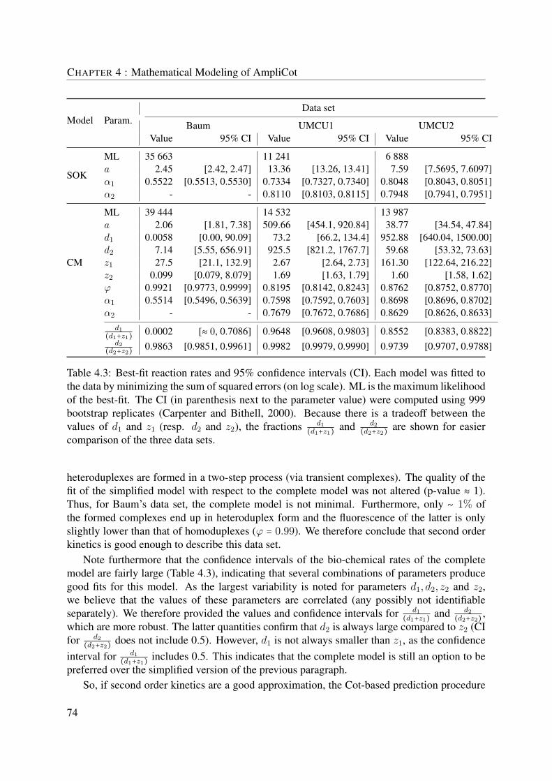
CHAPTER 4 : Mathematical Modeling of AmpliCot
Model Param.Data set
Baum UMCU1 UMCU2Value 95% CI Value 95% CI Value 95% CI
SOK
ML 35 663 11 241 6 888a 2.45 [2.42, 2.47] 13.36 [13.26, 13.41] 7.59 [7.5695, 7.6097]α1 0.5522 [0.5513, 0.5530] 0.7334 [0.7327, 0.7340] 0.8048 [0.8043, 0.8051]α2 - - 0.8110 [0.8103, 0.8115] 0.7948 [0.7941, 0.7951]
CM
ML 39 444 14 532 13 987a 2.06 [1.81, 7.38] 509.66 [454.1, 920.84] 38.77 [34.54, 47.84]d1 0.0058 [0.00, 90.09] 73.2 [66.2, 134.4] 952.88 [640.04, 1500.00]d2 7.14 [5.55, 656.91] 925.5 [821.2, 1767.7] 59.68 [53.32, 73.63]z1 27.5 [21.1, 132.9] 2.67 [2.64, 2.73] 161.30 [122.64, 216.22]z2 0.099 [0.079, 8.079] 1.69 [1.63, 1.79] 1.60 [1.58, 1.62]ϕ 0.9921 [0.9773, 0.9999] 0.8195 [0.8142, 0.8243] 0.8762 [0.8752, 0.8770]α1 0.5514 [0.5496, 0.5639] 0.7598 [0.7592, 0.7603] 0.8698 [0.8696, 0.8702]α2 - - 0.7679 [0.7672, 0.7686] 0.8629 [0.8626, 0.8633]
d1(d1+z1)
0.0002 [≈ 0, 0.7086] 0.9648 [0.9608, 0.9803] 0.8552 [0.8383, 0.8822]d2
(d2+z2)0.9863 [0.9851, 0.9961] 0.9982 [0.9979, 0.9990] 0.9739 [0.9707, 0.9788]
Table 4.3: Best-fit reaction rates and 95% confidence intervals (CI). Each model was fitted tothe data by minimizing the sum of squared errors (on log scale). ML is the maximum likelihoodof the best-fit. The CI (in parenthesis next to the parameter value) were computed using 999bootstrap replicates (Carpenter and Bithell, 2000). Because there is a tradeoff between thevalues of d1 and z1 (resp. d2 and z2), the fractions d1
(d1+z1)and d2
(d2+z2)are shown for easier
comparison of the three data sets.
heteroduplexes are formed in a two-step process (via transient complexes). The quality of thefit of the simplified model with respect to the complete model was not altered (p-value ≈ 1).Thus, for Baum’s data set, the complete model is not minimal. Furthermore, only ∼ 1% ofthe formed complexes end up in heteroduplex form and the fluorescence of the latter is onlyslightly lower than that of homoduplexes (ϕ = 0.99). We therefore conclude that second orderkinetics is good enough to describe this data set.
Note furthermore that the confidence intervals of the bio-chemical rates of the completemodel are fairly large (Table 4.3), indicating that several combinations of parameters producegood fits for this model. As the largest variability is noted for parameters d1, d2, z2 and z2,we believe that the values of these parameters are correlated (any possibly not identifiableseparately). We therefore provided the values and confidence intervals for d1
(d1+z1)and d2
(d2+z2),
which are more robust. The latter quantities confirm that d2 is always large compared to z2 (CIfor d2
(d2+z2)does not include 0.5). However, d1 is not always smaller than z1, as the confidence
interval for d1(d1+z1)
includes 0.5. This indicates that the complete model is still an option to bepreferred over the simplified version of the previous paragraph.
So, if second order kinetics are a good approximation, the Cot-based prediction procedure
74

4.3 Results
(which assumes the validity of SOK) should yield reasonable results, at least when applied tothe extrapolation of an unknown diversity close to the diversities of the calibration set. In orderto make predictions using the Cot-based method suggested in Baum and McCune (2006), theraw data were normalized by applying the transformation of Eq. (4.13) and the value of Cot0.5was estimated from the data and plotted as a function of the diversity n. The resulting plot(Figure 4.3) is a reproduction of Figure 2c of (Baum and McCune, 2006). The low diversitysamples (n = 1,2,5,10,30,48) are used to make a linear regression. The Cot 50% value of thesample with "unknown" diversity (n = 96) is then read on the y-axis of the plot and the value ofn at the intercept with the regression line is returned as the searched diversity. The confidenceinterval on the prediction is computed here from the confidence limits of the regression. Whenthe method is calibrated on the samples with diversities 1-48 (Figure 4.3A), the result of theCot-based prediction is n = 77, which is a ∼ 20% underestimation of the true diversity. Theconfidence interval ([69,87]) is rather large and it is not far from containing the true value.
0 50 96 150 2000
1
2
3
4
5
6
Diversity (n)
Cot
50%
Cot−based prediction using Cot 50%
Predicting n = 96...n* = 77, error = −19.79%CI = [69, 87]
77 0 50 96 150 2000
1
2
3
4
5
6
Diversity (n)
Cot
50%
Cot−based prediction using Cot 50%
Predicting n = 96...n* = 71, error = −26.04%CI = [69, 73]
71
A B
Figure 4.3: Cot-based prediction using Cot 50% of Baum&McCune’s data. The raw data hasbeen normalized using Eq. (4.13) and the value of Cot 50% is plotted as function of diversity.A linear regression (red solid line) is performed using the calibration set (○) and the intercept ofCot 50% of the "unknown" sample (●) with the regression line is used to make a diversity ex-trapolation (prediction). Dashed red lines: confidence interval of the regression. A: Calibrationon n = 1,2,5,10,30,48 gives a prediction of n = 77 (instead of 96), -20% error. B: Calibrationon n = 1,2,5,10,30 gives a prediction of n = 71, -26% error.
Nevertheless, the practical application of AmpliCot is to measure the diversity of T- or B-cell receptors, ranging in millions, by calibrating on a library of known diversities, orders ofmagnitude smaller. We are therefore interested in assessing the performance of the predictionmethods in conditions as close as possible to AmpliCot’s practical application. Hence, as a toyexample, we apply the Cot-based method to predict the highest diversity (n = 96) by calibratingon samples with diversities 1-30, thus omitting n = 48 (Figure 4.3B). The error of the resultingprediction has increased to 26% below the true value, while the confidence interval has shrunk([69,73]). Thus, the Cot-based method leads to underestimating the unknown diversity and the
75

CHAPTER 4 : Mathematical Modeling of AmpliCot
error is increasing with the gap between the most diverse calibration sample and the unknowndiversity. This questions the linearity of Cot values as function of n and consequently, the useof the Cot-based prediction method in practical situations.
4.3.3 The bias introduced by the use of SOK instead of CM has an im-
portant effect on predicting large diversities
We saw in the previous section that even though second order kinetics yielded a reason-able description of the data, the Cot-based prediction method, which is based on SOK, failedto provide correct diversity extrapolations. The systematic underestimation of the true diver-sity questioned the linearity of Cot vs n values. Intuitively, the underestimation suggests thatthe relationship is concave. If this is indeed the case, even a slight deviation from linearityon the scale of 1–100 diversities could introduce an important bias when extrapolating largediversities.
Having in mind that the CM gave a significantly better fit of the data, we investigated theshape of the tp(n) function under this model 3. To this end, we applied the transformationof Eq. (4.14) to the best-fit of the complete model, we estimated t0.5 and plotted it against n(Figure 4.4A, ●). For comparison, we also plotted on the same figure t0.5 of the data (◆) and ofthe SOK model (◾). As expected from theory, SOK exhibited a linear tp(n) relation, whereaslinearity was lost under the CM. Note that the deviation from linearity is small on the scale ofdiversities included in Baum’s data set (n ∈ [1,100]).
The initially small bias is however strongly amplified when considering large diversities.Figure 4.4B reveals that using one model, instead of the other, results in completely differentfunctions. In other words, the same t0.5 value has a completely different diversity-responseof the inverse t0.5(n) curve. Thus, this confirms the intuition that if the annealing kineticsare better approximated by the complete model, using the linear relation of second order ki-netics would largely underestimate the searched diversity. The next two sections describe theconsequences of the validity of the complete model.
4.3.4 Under the complete model, Cot scaling does not correct for concen-
tration differences
We address here the issue of concentration differences between samples. To understand theproblem, consider two samples of same diversity, say n = 1 for simplicity. Imagine that oneof them is twice the concentration of the other. Intuitively, in the more concentrated sample,molecules need to cover a smaller distance before meeting another molecule, so we expect thata higher concentration would result in a faster annealing.
Mathematically, the expression defining the annealing curve (Eq. (4.4)) under second orderkinetics contains the product Tt, i.e., the total concentration of DNA × time. This implies thatfor a given diversity, the same experiment performed with two different concentrations willresult in different annealing curves. In other words, two identical annealing curves plotted in
3. Note that we consider tp and not Cot values here, because Cot scaling can not be applied to the CM, asshown in Section 4.3.4.
76

4.3 Results
A B
0 20 40 60 80 1000
5
10
15
20
25
30
35
40
Diversity (n)
Second order kineticsComplete modelData
0 200 400 600 800 10000
50
100
150
200
250
300
350
400
Diversity (n)
Second order kineticsComplete modelData
t 0.5
t 0.5
Figure 4.4: Using the Cot-based prediction method that assumes SOK when reality is better ap-proximated by the complete model leads to underestimating large diversities. A: The behaviorof Cot 50% as function of n is computed using both models: second order kinetics (◾ solid) andthe complete model (● dashed). The parameters of the best-fit of Baum’s raw data have beenused. Cot 50% values estimated from the normalized data are also plotted (◆ dash-dotted). Forsmall diversities, the deviation from linearity is small. B: For larger diversities, the small biasbetween both models is amplified, leading to possibly wrong diversity predictions. Connectinglines are shown to help the visualization of the trend.
time scale do not necessarily imply the same sample diversity. This is a serious problem whenone wants to predict the diversity of a sample out of its annealing kinetics. The Cot scaling usedin (Baum and McCune, 2006) is a solution to this problem in the case of SOK, but it does notapply under the complete model (see Section 5.2 of Chapter 5 for a mathematical justification).
To illustrate the effect of a concentration change and Cot re-scaling, we have performed insilico experiments using both models. Figure 4.5A depicts the annealing kinetics of two virtualsamples, one having total nucleotide concentration of T1 = 1 (solid) and the other, concentrationT2 = 2 (dashed). The sample with highest concentration anneals faster, because moleculeencounters occur more frequently. The annealing curve of sample 2 (in time scale) is thereforeincreasing faster than the one of sample 1 (Figure 4.5A) although both samples have the samediversity (n = 40). In order to recover the same annealing curve for both samples, the annealingkinetics of sample 2 should be slowed down by multiplying time with the concentration. Theresult of Cot re-scaling is shown in Figure 4.5B, where both curves overlay perfectly.
In the case of the complete model, a Cot re-scaling can not compensate for concentrationdifferences, because the functions defining the ODE system of this model are not homoge-neous 4. A numerical example is shown in Figure 4.5C and D where the in silico experimentwas performed under the complete model. The Cot-scaled curves of Figure 4.5D do not overlay
4. A homogeneous function is a function with multiplicative scaling behavior: if the argument is multiplied bya factor, then the result is multiplied by some power of this factor. See Section 5.2 of Chapter 5 for a mathematicalillustration.
77

CHAPTER 4 : Mathematical Modeling of AmpliCot
0 20 40 600
0.2
0.4
0.6
0.8
1
Time
Ann
ealin
g cu
rve
SOK, T=1SOK, T=2
0 20 40 60 80 100 1200
0.2
0.4
0.6
0.8
1
Concentration x Time
Ann
ealin
g cu
rve
SOK, T=1SOK, T=2
0 20 40 600
0.2
0.4
0.6
0.8
1
Time
Ann
ealin
g cu
rve
CM, T=1CM, T=2
0 20 40 60 80 100 1200
0.2
0.4
0.6
0.8
1
Concentration x Time
Ann
ealin
g cu
rve
CM, T=1CM, T=2
A
C
B
D
Figure 4.5: Cot scaling is valid under second order kinetics, but can not correct for differencesin concentrations under the complete model. Annealing curves for two in silico experimentshaving different concentrations (T1 = 1 and T2 = 2). Top two panels: second order kineticsplotted on a time scale (A) and on a Cot scale (B). The curves in B overlay perfectly, showingthat the Cot scale corrects for the concentration differences. Bottom two panels: heteroduplexmodel on a time scale (C) and on a Cot scale (D). In this case, Cot scaling does not lead toan overlapping of the two curves. Parameters: best-fit parameters of Baum’s data (Table 4.3),n = 40.
perfectly as was the case under SOK. This is due to the fact that time does not appear solely ina product with the concentration in the solution of the complete model.
The correct way to handle concentration differences that is valid under both models, is byrescaling the association rates, as shown in Theorem 2 of Chapter 5.
4.3.5 Under the complete model, the function tp(n) is not linear
Here, we formalize mathematically the intuition of Section 4.3.3. The result presented hereapplies also to Cot values under second order kinetics, but because Cot scaling is not validunder the complete model, we derive it for tp values. Consider tp, p ∈ [0,1], the time point at
78

4.3 Results
which a proportion p of the sample has annealed. From the definition of the annealing curve(Eq. (4.14)), the latter is expressed as A(tp) = p. In the case of second order kinetics, tp is alinear function of diversity, as stated in Baum and McCune (2006). Indeed,
tp(n) = 1
2aα( p
1 − p)n, n ∈ N. (4.15)
This above expression was plotted in Figure 4.4 (p = 0.5).The linear relationship is lost under the complete model, as we saw in Figure 4.4 using the
numerical solution of the ODEs (Eq. (4.6)). An analytical expression of tp(n) under the CMis available in the particular case of a quasi-steady state (QSS) assumption. If the values of thereaction rates are such that the transient complexes C and H can be assumed in steady state,the ODE system is then easily solved (see Section 5.3.4 of Chapter 5 for a solution). From theresulting solution, one can derive the following expression:
tp(n) = pn
K1 +K2(n − 1) , n ∈ N,where
K1 = 2αa( z1d1 + z1
)(1 − p), K1 > 0
K2 = αa( z2d2 + z2
)(ϕ − p), K2 ∈ R.
Note that tp(n) is a rational (non-linear) function of n, except when p = ϕ. In that particularcase, K2 = 0 and tp(n) = pn/K1 is again linear, but this is not generally true.
4.3.6 Fitting other data sets suggests that SOK is not valid
In order to verify the validity of both models on other data sets, additional experiments wereperformed. We present two data sets, one containing diversities n = 1,4,8,16,32,48 and thesecond, n = 10,20,30,40. The fits of both models to these data sets are depicted in Figure 4.6(data set 1) and Figure 4.7 (data set 2). The improvement brought by the complete model wassignificant (p-value < 10−3) and this is especially clear when looking at the best-fit of the higherdiversity samples. We could clearly distinguish the time course of both models for n = 32 andn = 48 of data set 1, where SOK was unable to reproduce the correct curvature and the apparent“limit" value of the data. Moreover, SOK failed to give the correct asymptote value in the fit ofUMCU data set 2.
The best-fit parameters of the CM (Table 4.3) are very different from those of Baum’s data.For UMCU data set 1, the association and dissociation rates (a, d1, d2) of transient complexesare large compared to the polymerization rates z1 and z2. This suggests that a quasi-steady stateassumption for variables C and H can be applied to this data set. In this case, an analyticalsolution of the CM is available (see Section 5.3 of Chapter 5 for its derivation). For UMCUdata set 2, the QSS assumption can be valid too, but it seems less obvious in that case. In orderto verify if the assumption is applicable, one should compute and formally compare the twotime scales of the model, as done in Borghans et al. (1996).
79

CHAPTER 4 : Mathematical Modeling of AmpliCot
Time (min.)
Fluo
resc
ence
inte
nsity
(arb
itrar
y un
its)
n = 1 n = 4
n = 8 n = 16
n = 32 n = 48
−20 0 20 40 60
102.1
102.3
102.5
102.7
−20 0 20 40 60
102.1
102.3
102.5
102.7
102.9
−20 0 20 40 6010
2.1
102.3
102.5
102.7
102.9
−20 0 20 40 60
103
−20 0 20 40 60
103
−20 0 20 40 60
103
Figure 4.6: Best-fit of UMCU data set 1 for known diversity templates (each panel). Solidblue: data sample (t < 0: pre-anneal phase, t ≥ 0: annealing phase). Dashed blue: the inferredkinetics of the "unmelted" sample, as predicted by the model. Black: reference. Solid green:best-fit of SOK. Solid red: best-fit of the CM. For color references, please consult the onlineelectronic version of the thesis.
80

4.3 Results
Time (min.)
Fluo
resc
ence
inte
nsity
(arb
itrar
y un
its)
n = 10 n = 20
n = 30 n = 40
−50 0 50 100 15010
2
103
−50 0 50 100 15010
2
103
−50 0 50 100 15010
2
103
−50 0 50 100 15010
2
103
Figure 4.7: Best-fit of UMCU data set 2 for known diversity templates (each panel). Solidblue: data sample (t < 0: pre-anneal phase, t ≥ 0: annealing phase). Dashed blue: the inferredkinetics of the "unmelted" sample, as predicted by the model. Black: reference. Solid green:best-fit of SOK. Solid red: best-fit of the CM. For color references, please consult the onlineelectronic version of the thesis.
Similarly to Baum’s data, we remark that the confidence intervals of the composite param-eter d2
(d2+z2)are very tight around 0.99 for UMCU1 and around 0.97 for UMCU2. Hence, d2 is
always large with respect to z2, indicating that a large proportion of complexes fall apart beforedefinitely associating. Contrary to Baum’s data, the same is true for d1 and z1 of UMCU datasets (d1 is always large with respect to z1).
Note that we have fitted two values for the proportion of single-stranded material at the start
81

CHAPTER 4 : Mathematical Modeling of AmpliCot
of the annealing (α1 and α2), each corresponding to samples of the same row. α1 correspondsto the samples placed on the extremity of the plate, i.e., those that were melted at the highesttemperature. We therefore expect that in these samples, the material melts somewhat faster,which would lead to a higher α value (α1 > α2). This is indeed the case for UMCU2 dataset, but not for UMCU1. In fact, even though both best-fit values are very close to each other(α1 = 0.7598, α2 = 0.7679), their confidence intervals do not overlap which indicates that bothvalues are significantly different. This counter-intuitive result, together with the fact that thebest-fit values of α1 and α2 are very close to each other, suggests that the model can be furthersimplified by imposing one single α parameter for all replicates.
Finally, the best-fit parameters indicate that the fluorescence of heteroduplexes was esti-mated to be only 80-90% of that of homoduplexes (ϕ = 0.82 for data set 1, ϕ = 0.89 for dataset 2), which contrasts with Baum’s data where the few heteroduplexes could have almost thesame fluorescence as homoduplexes.
4.3.7 Diversity-dependent fluorescence loss
We discuss here a phenomena that is typically observed in AmpliCot assays. Once theannealing has been completed, it has been often remarked that samples do not reach their pre-anneal values (even after correction for the slow fluorescence decay). This leads to a gap asshown in the example of Figure 4.8A. We define the gap as the difference between the inferredunmelted sample and the "limit" values of the annealing samples, predicted by the model. By“limit" values, we mean that the model is executed for a long time-period (for example 10hours) with the best-fit parameters of the corresponding data set. Thus, the model is used tosimulate a very long experiment in which all the material re-anneals (t → ∞). A diversity-dependent gap is then observed in the three data sets (Figure 4.8B and C).
B C
−50 0 50 100 15010
2
103
}}gap1gap2
A
Time (min.)
Flu
ores
cenc
e in
tens
ity
0 20 40 60 80 1000
0.5
1
1.5
2
2.5
3
3.5x 10
−3
Diversity
Gap
0 10 20 30 40 500
10
20
30
40
50
60
70
Diversity
Gap
UMCU1
UMCU2
Baum&McCune
Figure 4.8: Diversity-dependent fluorescence loss. A: The fluorescence gap is defined as thedifference between the inferred unmelted sample (dashed lines) and the "limit" measured valuesof the annealing samples (solid lines) (in this example: n = 40 of UMCU data set 2, bothreplicates). The gap increases with diversity. B: Baum & McCune’s data, C: UMCU data sets1 and 2 (●: replicate 1, ◾: replicate 2). The correlation coefficients and their p-values are in thelegends.
82

4.3 Results
The same property was observed to a greater extent in Schütze et al. (2010). The authorsof this study constructed samples with very large and known diversities (up to 1012 differentsequences). When they applied the AmpliCot protocol to their oligonucleotide library, despitethe prolonged annealing times (up to 6h.), the fluorescence of samples with diversity 106 andabove stayed well below 50% of its initial value. The authors were therefore unable to mea-sure the Cot 50% value necessary for applying the Cot-based prediction method. Hence, assuggested by their Figure 2(a), high diversities seem to be associated with a systematic loss offluorescence.
Contrary to second order kinetics, which implies that a sample should always reach its pre-anneal fluorescence level after re-annealing, the complete model is compatible with the aboveobservations. We hypothesize that the diversity-dependent fluorescence loss is caused by thepresence of heteroduplexes, which have a decreased fluorescence intensity.
4.3.8 Fluorescence Intensity for Very Large n
In the previous section, we saw that the fluorescence gap is increasing with diversity. Inother terms, the limit fluorescence intensity is inversely correlated with diversity. Here, weinvestigate the lower bound of the fluorescence, i.e., we study the fluorescence intensity forvery large diversities. The question that we want to answer is "Would the samples with verylarge diversity loose all their fluorescence?" This is of interest, because AmpliCot is designedto estimate the diversity of TCRs that is orders of magnitude larger than the “toy" data sets ofour study.
By using the analytical solution of the CM under a quasi-steady state assumption (Sec-tion 5.3), we can derive the time-limit fluorescence intensity F ∗(n) as a function of diversity:
F ∗(n) ∶= limt→∞
F (t) = 2(D∗(n) +ϕJ∗(n)),where D∗(n) and J∗(n) are given by Eq. (5.21) and Eq. (5.20) of Chapter 5.
As n increases, the fluorescence level is decreasing and has limit value
F ∶= limn→∞
F ∗(n) = 1 − (1 −ϕ)α. (4.16)
(See also Eq. (5.24) of Chapter 5 for derivation details.) The expression of F (Eq. (4.16))contains parameters ϕ and α, i.e., the fluorescence intensity of heteroduplexes and the initialproportion of melted material, respectively. Let us examine the values of these parametersin order to determine the lower bound of the fluorescence intensity for very diverse samples.There are four extreme cases of ϕ and α, which lead to three distinct values of F :
(i) ϕ = 1 or α = 0 ⇒ F = 1(ii) ϕ = 0 ⇒ F = 1 − α(iii) α = 1 ⇒ F = ϕPoint (i) is trivial: if heteroduplexes fluoresce as much as homoduplexes (ϕ = 1), the CM
is reduced to a variant of SOK where the DNA association occurs in two steps (heteroduplexesare not distinguished from homoduplexes) and hence the fluorescence level after re-annealingwould reach its pre-anneal initial value (F = 1); the case α = 0 means that none of the materialhas melted, which is unrealistic.
83

CHAPTER 4 : Mathematical Modeling of AmpliCot
Point (ii) means that if heteroduplexes do not fluoresce (ϕ = 0), very diverse samples wouldloose most of their fluorescence and the only remaining fluorescent material, if any, would bethe proportion 1 − α of unmelted homoduplexes. This can also be seen from the individualcontributions of homo- and hetero- duplexes (see Figure 5.2 of Chapter 5). As n increases, theproportion of heteroduplexes reaches the limit value α (Eq. (5.23)), whereas the only remaininghomoduplexes are those that have not dissociated during the melting step. Hence, if heterodu-plexes do not fluoresce, an "ideal" experiment in which the all the material melts (α = 1) wouldresult in the quasi-total loss of fluorescence in very diverse samples (F → 0).
Symmetrically, point (iii) indicates that in an "ideal" experiment where the all the materialmelts (α = 1), there would be only heteroduplexes at the end of the annealing and the maximalfluorescence would be given by their fluorescence (F = ϕ).
4.3.9 Diversity Predictions
In order to improve the diversity extrapolations of AmpliCot, we propose here two alter-natives to the Cot-based prediction method: the model-based and the tp-based methods. Bothprocedures take advantage of the following results of our modeling:
– The CM is a better description of AmpliCot than SOK;– Cot scaling does not correct for concentration differences;– The relation tp vs n is not linear.
The model-based method is based on the first result above. It uses not only the informationof the annealing curves sampled at one point as in the Cot-based procedure, but the informationcontained in the entire annealing curve. It also has the advantage of using directly the raw data,which avoids the introduction of bias and the loss of information due to normalization. Themodel-based method uses the samples of known diversity to fit the parameters of the underlyingannealing kinetics model. The biochemical reaction rates are then fixed to their best-fit valuesand a range of possible values for the unknown diversity is determined. For each value of nin this pre-determined set, the remaining parameters (Ωi, Eq. (4.12)) are fitted to the samplewith unknown diversity by minimizing the squared errors. The log-likelihood of the resultingfit is calculated. The unknown diversity is estimated as the value of n that maximizes thelog-likelihood (see Table 4.2 for a summary of all prediction methods).
The tp-based method is a modified version of the Cot-based one. It uses the second andthird results above. Similarly to the Cot-based procedure, it samples the data at a single point(which has to be chosen a priori), but instead of assuming a linear relation between tp and n, ituses the best-fit of the complete model to infer the (possibly nonlinear) relation. The unknowndiversity is read from the relation t−1p (t). The advantage of this method with respect to themodel-based one is to ignore the regions of the annealing curve where the model does not fitthe data well. The drawback is that one has to choose a “good" tp value (we discuss this topicin Section 4.3.10).
In order to compare their performance, we have applied the three prediction methods toBaum’s data and to UMCU data set 1. All but the two largest diversity samples were used forcalibration (n = 1,2,5,10,30 for Baum’s data, n = 1,4,8,16 for UMCU data) and the goalwas to predict the largest diversity (n = 96 for Baum’s data, n = 48 for UMCU data). UMCU
84

4.3 Results
data set 2 was left out, because it contained too few diversities for the calibration set. Table 4.4displays the results of the prediction experiments. The confidence intervals were computed bybootstrapping the calibration sets, as explained in Section 4.2.11.
Method Data set Prediction Error 80% CI
Cot-based (50%)Baum 71 -26.04% [71, 75]UMCU 1 36 -25.00% [31, 38]
Cot-based (80%)Baum 86 -10.42% −∗UMCU 1 62 +29.17% [59, 73]
Model-basedBaum 94 -2.00% [61, 135]UMCU 1 53 +10.00% [39, 53]
tp-based (85%)Baum 97 +1.04% [73, 129]UMCU 1 45 -6.25% −∗
Table 4.4: Prediction results. The three methods are described in Table 4.2. All methods werecalibrated on all but the two largest diversity samples. The diversity to predict was n = 96for Baum’s data and n = 48 for UMCU data. The confidence intervals (CI) were computedby bootstrapping the calibration data sets (see Section 4.2.11). The error is expressed as thepercentage from the true diversity. ∗The CI could not be computed because the distribution ofbootstrap replicates exhibited a bi-modal shape (see Figure 4.9).
When comparing the predictions obtained by the Cot-based method with those of the model-based one, we observe an impressive improvement in the case of Baum’s data, although thisdata set was nicely explained with SOK. Indeed, the error in the estimation of the diversityis reduced more than 10 times, passing from 26% to 2% underestimation. The improvementis more moderate in the case of the UMCU data: the error is reduced a bit more than twice,passing from 25% underestimation to 10% overestimation. Using the 80% annealing pointinstead of 50% in the Cot-based method improves the predictions of Baum’s data, but not ofthe UMCU data. For the tp-based method, we show here the results with the highest possibleannealing percentage (85%). It turns out that this method gives the smallest prediction errorfor both data sets. The prediction is now within 10% from the true value and the improvementfrom the initial Cot 50% method is about 5-fold. Thus, the new prediction methods seem toyield good results. This was indeed expected, as these methods use more data information thanthe Cot-based method.
However, the confidence intervals of the predictions reveal a very large variability aroundthe values predicted by the model-based and tp-based methods. Nevertheless, these confidenceintervals contain the true diversity, which is not the case for the Cot-based method. To furtheranalyze the performance of the prediction methods, we have plotted the histograms of boot-strapped predictions (Figure 4.9). Each prediction method was applied toR bootstrap replicatesand the histogram of resulting diversity estimations is shown (these distributions were used forthe confidence intervals estimations). The true diversity values are indicated by a dashed verti-cal line. We note that the density of predictions of the Cot-based method (both for p = 0.5 and
85

CHAPTER 4 : Mathematical Modeling of AmpliCot
70 75 80 85 90 95 1000
1000
2000
3000
4000Cot−based, p=0.5
50 60 70 80 90 1000
500
1000
1500
2000Cot−based, p=0.8
0 50 100 150 2000
100
200
300
400Model−based
50 100 150 2000
50
100
150
200tp−based, p=0.85
0 10 20 30 40 500
1000
2000
3000
4000Cot−based, p=0.5
0 20 40 60 80 1000
500
1000
1500
2000
2500Cot−based, p=0.8
0 20 40 60 80 1000
50
100
150
200Model−based
20 30 40 50 60 70 800
50
100
150tp−based, p=0.85
R = 4999 R = 4999
R = 4999 R = 4999
R = 1603 R = 630
R = 728 R = 500
A
B
C
D
E
F
G
H
Figure 4.9: Bootstrap distributions. The Cot-based (first and second row of panels), model-based (third row of panels) and the tp-based method (last row of panels) were executed onbootstrap replicates of the calibration sets of Baum’s data set (panels A-D) and UMCU dataset 1 (panels E-F). The histograms of the resulting predictions are plotted. The search diversityis indicated by the red dashed vertical line. The effective number of bootstrap replicates R isindicated in the upper left corner of each plot. Although the new methods are very sensitive,their distribution is centered around the true diversity.
86

4.3 Results
0.8, panels A,B,E,F) are far from the true diversity. Remark moreover the bimodal distribu-tion of panel B, which indicates that the Cot-based method applied on Baum’s data can yield areasonable diversity prediction. The model-based and the tp-based methods have densities cen-tered around the true value. Again, a bimodal distribution is revealed by the tp-based methodapplied on UMCU data set 1 (panel H), which prevented us from computing a confidence in-terval. Note that predicting a diversity from a bootstrap replicate is rather challenging becausewith high probability, the calibration set contains less diversities than the original calibrationset. This can explain why the methods that involve more parameters (the model- and tp-based)exhibit distributions with larger variance.
4.3.10 Criteria for Choosing a Correct Annealing Percentage
The Cot- and the tp-based prediction methods have one parameter, the annealing percentagep, that needs to be set before applying the procedure. A last question remains: how to choosean annealing percentage such that the prediction errors are minimized? Here, we investigate thedependence of the prediction on the chosen value of p. Figure 4.10 shows this dependence forboth data sets (Baum: A, UMCU: B) and for both prediction methods. Note that the Cot-basedmethod assumes second order kinetics, whereas the tp-based method is based on the completemodel.
tp-based method
Cot−based method
A B
tp-based method
Cot−based method
0.2 0.3 0.4 0.5 0.6 0.7 0.8 0.9−60
−40
−20
0
20
40
60
Annealing percentage (p)
Pre
dict
ion
erro
r (%
)
0.2 0.3 0.4 0.5 0.6 0.7 0.8 0.9−60
−40
−20
0
20
40
60
Annealing percentage (p)
Pre
dict
ion
erro
r (%
)
Figure 4.10: Prediction error as function of the annealing percentage. The Cot- (resp. tp-)based method was executed with different values of p and the prediction error was computed.A: Baum’s data, calibration on n = 1,2,5,10,30, predicting n = 96, B: UMCU data set 1,calibration on n = 1,4,8,16, predicting n = 48.
For Baum’s data, the tp-based method is in general producing a smaller error than the Cot-based version (except for values of p below 40%). In general, for both methods, it seems thatthe prediction is improving as the annealing percentage is increasing. In fact, both methodsgive similar predictions for Cot values above 80%. This is not the case for UMCU data (Fig-ure 4.10B). For this data set, the tp-based method has a more "chaotic" behavior, but it stillseems that higher annealing percentages result in better predictions.
87

CHAPTER 4 : Mathematical Modeling of AmpliCot
We searched for criteria that would guide the choice of annealing percentage from the cali-bration set, before making a diversity extrapolation. In other words, we aimed to find the regionof the data that contains most information about the diversity and that can be inferred from thecalibration data set.
For the tp-based method, a possible candidate would be the quality of the fit. As we sawin Figure 4.2, the complete model fits some parts of the annealing curve better than others.For example, the first 10 minutes of Baum’s experiment are not very well explained with ourmodel, thus we would like to avoid the annealing percentages corresponding to that region.To see whether there is a positive correlation between the sum of squared errors (SSE) aroundan annealing percentage p and the prediction error, we have plotted the latter quantities (Fig-ure 4.11). There is clearly a positive correlation between both variables (corr. coeff. = 0.83 forBaum’s data, 0.67 for UMCU data), thus confirming that in general, a good fit implies a goodprediction. However, the relation is not really linear (especially for Baum’s data) and very goodpredictions can be obtained with not-so-good fits. Nevertheless, if we use the annealing pointat which the SSE is minimal (p = 0.85 for Baum’s data, and p = 0.47 for UMCU data, figurenot shown), we obtain a reasonably low error in the estimate of the diversity (+1.05% for Baumand +12.5% for UMCU).
0 0.5 1 1.5 2 2.5 3
x 10−3
0
5
10
15
20
25
30
35
40
45
Mean SSE
| Pre
dict
ion
erro
r | (
%)
0 1 2 3 4 5 6 7
x 10−3
0
10
20
30
40
50
60
70
80
90
100
Mean SSE
| Pre
dict
ion
erro
r | (
%)
A B
Corr. coeff: 0.67p-value: 2.9e-9
Corr. coeff: 0.83p-value: 2.2e-16
Figure 4.11: Mean sum of squared errors (SSE) vs prediction error. The tp-based method wasexecuted with different values of p. The quality of fit at the value of p, in terms of the mean SSE,is plotted horizontally; the absolute value of the relative prediction error is plotted vertically.A: Baum’s data, B: UMCU data set 1. A significant positive correlation is observed.
For the Cot-based method, a possible rule could be the quality of the linear regression (interms of theR2 statistic). However, we did not find a positive correlation between the latter andthe prediction error. Therefore, we recommend to try the Cot-based method with several Cotvalues in order to test the sensitivity of the technique to these values. A higher Cot value cangive better results, but according to our analysis, it is not guaranteed.
88

4.4 Discussion
4.4 Discussion
By means of a mathematical model, we analyzed and improved the interpretation of Am-pliCot (Baum and McCune, 2006). We showed that the initially assumed underlying model,second order kinetics, is not always the best to describe the annealing dynamics. We proposean alternative, the complete model, which considers the biochemical reaction in further detail.The consequences of using this alternative model are twofold: the Cot scaling that was appliedunder SOK to account for concentration differences between samples is no longer applicable,and the relation between tp values and diversity is no longer linear. These facts have casteddoubt on the accuracy of the diversity extrapolation approach based on second order kinetics.As a solution, we have proposed two alternative prediction methods that take into account thefindings of our modeling.
Our model-based prediction method has several advantages over the Cot-based one. It isindependent on a single annealing percentage, because it considers the entire annealing curve inorder to extrapolate the necessary information. Thus, it uses the full data set, not only a subsetof it. It also yielded good prediction results when applied to the extrapolation of a sample withdiversity at least 3 times larger than the diversities of the calibration set.
A possible drawback of our approach would be its sensitivity to the correct estimation ofthe bio-chemical reaction rates. As we saw, the confidence limits of the parameter estimatesare sometimes large (Table 4.3), suggesting that some parameters might not be separately iden-tifiable. A solution to that problem could be to fit directly the combined parameters d1
(d1+z1)and
d2(d2+z2)
.Another source of inaccuracy might appear on the level of the “diversity fitting" itself. Once
the best-fit reaction rates are found, the diversity extrapolation procedure consists in iteratingover a pre-determined range of diversities n ∈ N and fitting the remaining curve-specific pa-rameters (see Table 4.2 for a summary of the procedure). The value of n that maximizes thelikelihood of the unknown diversity sample is chosen as the searched diversity n∗. A legiti-mate question is whether the optimal value n∗ is a global maximum of the likelihood function?In other words, can we identify n given the best-fit values of the reaction rates? To addressthis issue, we have artificially generated data according to both models (SOK and the CM) byadding random noise to the numeric solution of the ODEs of Eq. (4.3) or Eq. (4.5) (data notshown). The artificial data was then used to perform the prediction experiments in the sameway it was performed with the real data. When the same model was used to generate and tofit the artificial data, the resulting predictions were 100% accurate. This indicates that once theparameter values are found by the fitting procedure, there is an unique value of n for whichthe likelihood of the data set with unknown diversity is maximal. Note that this is true for anuniform species distribution, but it might not be true in presence of expanded clones.
A parameter that strongly influences the output of the model is the baseline fluorescenceof a sample (Ab). This parameter determines the post-annealing fluorescence level, which,in turn, determines the value of ϕ, the fluorescence intensity of heteroduplexes (and maybeeven the reaction rates determining the fraction of heteroduplexes). In order to obtain the bestpossible estimates of Ab, our approach requires long enough pre-anneal measurements. Thiswas not the case with Baum & McCune’s raw data, where the pre-anneal values lasted for
89

CHAPTER 4 : Mathematical Modeling of AmpliCot
only 10 minutes. The problem with such short measurements is the possible instability ofthe fluorescence intensity, as seen in this data set. A clear example of this instability can beseen in the sample of diversity n = 1 (Figure 4.2). Indeed, the fluorescence intensity clearlyincreases during the pre-anneal measurements, whereas a slow decline is expected due to dyedegradation. These transient instabilities are influencing the estimation of Ab and thus addingnoise to the rest of the parameter estimates. Good estimates of Ab are needed as well for thenormalization transformation (Eq. (4.13)), hence we recommend that pre-anneal measurementsshould last long enough (at least 20-30 minutes).
Another issue related to the estimation of Ab, but also to other parameters, is the timeinterval between the true beginning of the annealing and the first measurement (we call thistime interval Δ). We assume that we know the initial conditions of the ODE system at thebeginning of the annealing phase, but the first available measurement is some time after thestart of the annealing. If this time lapse (Δ) is large, it might influence the estimation of thereaction rates. Parameter Δ also influences the value of the limit fluorescence ϕ, because Ab,which is determined by the last pre-anneal measurements, is corrected for the time-dependentfluorescence decay between the last pre-anneal point and the first annealing measurement. Itis therefore important to have a precise knowledge of this time gap. In order to obtain thebest-possible parameter estimates, we tried adding Δ to both models as an unknown parameterto be fitted. However, as the resulting best-fit values of Δ turned out to be small (less thana minute for all data sets), for simplification, we have removed this parameter from our mainmodel description.
The complete model was able to explain the fact that the re-annealed samples do not reachtheir pre-anneal fluorescence intensity, even after correction for the fluorescence decline dueto dye degradation, as was noted in Schütze et al. (2010). We suggest that this is due to thepresence of heteroduplexes which have a lower fluorescence than homoduplexes. An alterna-tive explanation of this phenomena would be that as the annealing temperature is very close tothe melting one, the formed homoduplexes dissociate and re-associate again. We have fittedsuch a model to the data and although it accounted for the above-mentioned fluorescence gap,this model did not explain the beginning of the annealing curves and therefore yielded a signif-icantly lower quality of the fit with respect to the complete model. An alternative explanationof the fluorescence gap could be a diminished efficiency of the SYBR green die after melting.However, this would not explain the diversity-dependence of the gap.
An important issue that was not addressed at this stage is the effect of expanded clones. Westudied here only the case of an uniform distribution of species, which allowed us to reducethe dimension of the ODE systems. This resulted in a computationally efficient definition ofthe models, independent of the number of species. The equimolarity assumption is probablyvalid for naive T cells, but its validity is lost in the case of antigen-primed T cell populations(Naumov et al., 2003), although it was recently shown that the human memory repertoire iscomposed of a majority of low frequency clones (Klarenbeek et al., 2010). Nevertheless, theuse of AmpliCot in the presence of even one expanded clone becomes more tricky. If a samplecontains one or several expanded clones, the annealing kinetics of this sample would behaveas if its diversity is lower. Fitting the complete model might become very complex in thatsituation and further analysis is needed in order to make a conclusion. In such cases, readingthe annealing curves at a single point as close to completion as possible, as suggested in Baum
90

4.4 Discussion
and McCune (2006), would be the best solution at this moment.Finally, in addition to the development of methods dealing with non-equimolar samples, it
would be of interest to validate our current results with samples of diversity higher than 100species.
91

CHAPTER 4 : Mathematical Modeling of AmpliCot
92

Chapter 5Analysis of the AmpliCot Model
In Chapter 4, we defined two models describing the annealing kinetics of AmpliCot, namelysecond order kinetics (SOK) and the complete model (CM) (Section 4.2.3). In this chapter, wederive the theoretical results necessary for the analysis of these models. In Section 5.1, weformally expose the correct way of handling concentration differences under the CM. We thenrigorously show why Cot scaling is not valid under the CM (Section 5.2). Finally, we presentin Section 5.3 an analytic solution of the CM, valid in the particular case of a quasi-steady stateassumption (QSS).
5.1 Handling Concentration Differences
The theorem exposed in this section shows that comparing samples with different concen-trations affects the association rates. In fact, correcting the association rates is an alternative toCot scaling in accounting for the concentration differences between samples. The advantage isthat this correction can be used with both models, not only with second order kinetics.
Before giving the theorem, we introduce a general framework for describing the models.The differential equations can be written as:
dx(t;Θ, T )dt
= F (x,Θ), (5.1)
x(0;Θ, T ) = T ∗ (f , 0m−n)′where f = (f1, f2, . . . , fn) is the vector giving the proportion of each DNA type inside thesample (∑n
i=1 fi = 1), 0m−n = (0,0, . . . ,0) is the zero vector of dimension 1 × (m − n), m is thenumber of state variables, n is the sample diversity, and x, Θ and F (⋅) are defined differentlyaccording to the model.
We split the parameters in two groups, Θ ∶= (θ1, θ2), in order to distinguish the parametersthat have units depending on the concentration (θ1 = a) from those having time-dependent units(θ2 = (d1, d2, z1, z2)).Theorem 2. The normalized dynamics of a sample with total concentration of ssDNA S0 =γ ≠ 1 and reaction rates Θ = (θ1, θ2) are equivalent to the dynamics of a sample with total
93

CHAPTER 5 : Analysis of the AmpliCot Model
concentration of ssDNA S0 = 1 and reaction rates Θ = (γθ1, θ2). Mathematically,
x(t; θ1, θ2, γ)γ
= x(t;γθ1, θ2,1).Proof. Let
y(t; θ1, θ2, γ) ∶= γx(t;γθ1, θ2,1). (5.2)
We will show that y satisfies the same differential equation as x(t; θ1, θ2, γ), which is
d
dtx(t; θ1, θ2, γ) = F (x(t; θ1, θ2, γ), θ1, θ2) (5.3)
x(0; θ1, θ2, γ) = γ(f , 0m−n) (5.4)
For the initial conditions, we have by definition:
y(0; θ1, θ2, γ) = γx(0;γθ1, θ2,1)= γ(f , 0m−n)′= x(0; θ1, θ2, γ).Then, using the definition of y(⋅),
d
dty(t; θ1, θ2, γ) = γ
d
dtx(t;γθ1, θ2,1)= γF (x(t;γθ1, θ2,1), γθ1, θ2)
Eq. (5.2)= γF (1γy(t; θ1, θ2, γ), γθ1, θ2)= F (y(t; θ1, θ2, γ), θ1, θ2),
where the last equality holds for both models. Indeed, we show below that it is true for thefunction F in the case of the complete model and therefore, it is also true for SOK, as it is asubset of the former. Let F (⋅) = (F1(⋅), . . . , F1(⋅)), where F1(⋅), . . . , F1(⋅) are the right-handsides of the system of Eq. (4.2). We have
γF1 (1γy(t; θ1, θ2, γ), γθ1, θ2) = γ (−2aγS2
i
γ2− aγ
Si
γ∑j≠i
Sj
γ+ 2d1
Cii
γ+ d2 ∑
j≠i
Cij
γ)
= −2aS2i − aSi ∑
j≠i
Sj + 2d1Cii + d2 ∑j≠i
Cij
= F1(y(t; θ1, θ2, γ), θ1, θ2)and similarly for F2, F3 and F4.
The function F (y,Θ) being continuous in y and having continuous first partial derivativeswith respect to y, there is a unique solution to the initial value problem of Eq. (5.3). There-fore, as y(⋅) is a solution of the differential equation Eq. (5.3), we must have y(⋅) ≡ x(⋅), i.e.,x(t; θ1, θ2, γ) = γx(t;γθ1, θ2,1), which proves the theorem.
Theorem 2 means that normalized data should not be fitted with unique association rates θ1for all diversity samples, but sample i should have association rate γiθ1, where γi is an estimateof the total concentration of sample i.
94

5.2 Cot Scaling is Only Valid under Second Order Kinetics
5.2 Cot Scaling is Only Valid under Second Order Kinetics
Consider the differential equations defining second order kinetics:
dSi
dt= −2aS2
i (5.5)
dDii
dt= aS2
i ,
i = 1, . . . , n. In compact form, these can be written as
dx
dt= F (x(t)), (5.6)
where x = (S1, . . . , Sn,D11, . . . ,Dnn)′ is a solution of Eq. (5.6). Let
y(t) ∶= Tx(Tt), (5.7)
i.e., a Cot re-scaled system with total concentration T . Differentiating Eq. (5.7) with respect tot yields
dy
dt= T 2dx
dt(Tt) = T 2F (x(Tt)) (5.8)
In the case of second order kinetics (Eq. (5.5)), F is a homogeneous function, i.e., F (Tt) =T 2F (Tt). Indeed, we have
F
⎛⎜⎜⎜⎜⎜⎜⎜⎜⎝
S1(t)⋮Sn(t)D11(t)⋮Dnn(t)
⎞⎟⎟⎟⎟⎟⎟⎟⎟⎠=
⎛⎜⎜⎜⎜⎜⎜⎜⎜⎝
−2aS1(t)2⋮−2aSn(t)2aS1(t)2⋮aSn(t)2
⎞⎟⎟⎟⎟⎟⎟⎟⎟⎠and
F
⎛⎜⎜⎜⎜⎜⎜⎜⎜⎝
TS1(Tt)⋮TSn(Tt)TD11(Tt)⋮TDnn(Tt)
⎞⎟⎟⎟⎟⎟⎟⎟⎟⎠=
⎛⎜⎜⎜⎜⎜⎜⎜⎜⎝
−2aT 2S1(t)2⋮−2aT 2Sn(t)2aT 2S1(t)2⋮aT 2Sn(t)2
⎞⎟⎟⎟⎟⎟⎟⎟⎟⎠= T 2F (x(Tt)).
Therefore,dy
dt= T 2F (x(Tt)) = F (Tx(Tt)) = F (y(t)),
meaning that y(t) is also a solution of Eq. (5.6). Thus, Cot scaling is correcting for concentra-tion differences under second order kinetics.
Cot scaling is not valid for the complete model, because the function F defining the systemis not homogeneous.
95

CHAPTER 5 : Analysis of the AmpliCot Model
5.3 Analysis of the CM under a QSS Assumption
We present an analytical solution of the complete model in the particular case of a quasi-steady state (QSS) assumption. Such an assumption is valid if the association and dissociationrates (a, d1, d2) of transient complexes are large compared to the polymerization rates z1 and z2(alternatively, if there are two time scales in the dynamics (Borghans et al., 1999)). By applyingthe QSS assumption, we can solve the ODE system (Section 5.3.1) and find equilibrium points(Section 5.3.2). The solution is further used to the fluorescence intensity for large diversitysamples (Section 5.3.3) and to derive an analytical expression of tp(n) (Section 5.3.4).
5.3.1 Complete Model Solution
The following system of differential equations defines the complete model (assuming equimo-lar distribution of species):
dS
dt= −a(n + 1)S2
n+ 2d1C + 2d2H (5.9)
dC
dt= a
S2
n− (d1 + z1)C (5.10)
dH
dt= a(n − 1
2) S2
n− (d2 + z2)H (5.11)
dJ
dt= z2H (5.12)
dD
dt= z1C, (5.13)
with initial conditions S(0) = αT , 2D(0) = (1 − α)T , C(0) = H(0) = J(0) = 0, and conserva-tion law
S(t) + 2(C(t) +H(t) +D(t) + J(t)) = T. (5.14)
If the association/dissociation rates a, d1, d2 of transient complexes C(t) andH(t) are largecompare to the final duplex formation rates z1 and z2, we can assume that the transient com-plexes reach quickly a steady-state. By setting their corresponding time-derivatives (Eq. (5.10)and Eq. (5.11)) to 0, we get:
C = a
n(d1 + z1)S2 (5.15)
H = a
n(d2 + z2) (n − 1
2)S2 (5.16)
By inserting Eq. (5.15) and Eq. (5.16) in the initial system, we get:
dS
dt= −2K(n)S2
dJ
dt= a
n( z2d2 + z2
)(n − 1
2)S2 (5.17)
dD
dt= a
n( z1d1 + z1
)S2,
96
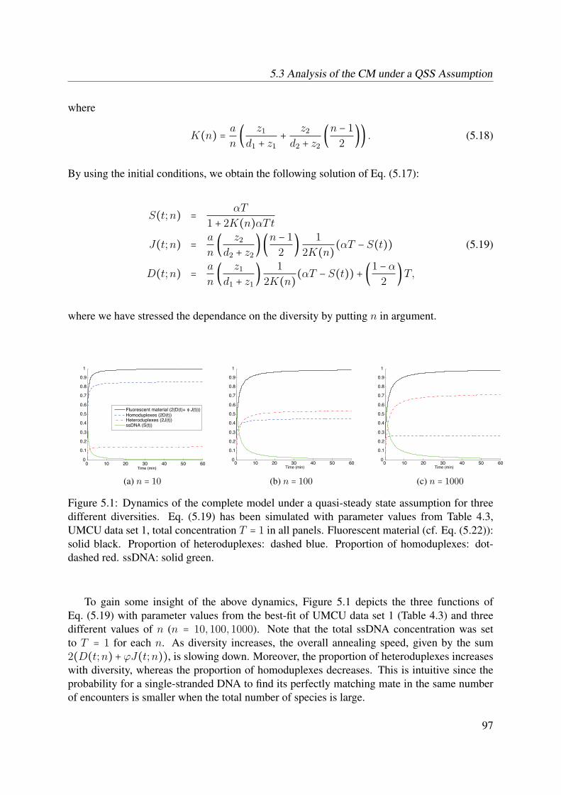
5.3 Analysis of the CM under a QSS Assumption
where
K(n) = a
n( z1d1 + z1
+ z2d2 + z2
(n − 1
2)) . (5.18)
By using the initial conditions, we obtain the following solution of Eq. (5.17):
S(t;n) = αT
1 + 2K(n)αTtJ(t;n) = a
n( z2d2 + z2
)(n − 1
2) 1
2K(n)(αT − S(t)) (5.19)
D(t;n) = a
n( z1d1 + z1
) 1
2K(n)(αT − S(t)) + (1 − α
2)T,
where we have stressed the dependance on the diversity by putting n in argument.
0 10 20 30 40 50 600
0.1
0.2
0.3
0.4
0.5
0.6
0.7
0.8
0.9
1
Time (min)
Fluorescent material (2(D(t)+ φ J(t)))Homoduplexes (2D(t))Heteroduplexes (2J(t))ssDNA (S(t))
(a) n = 10
0 10 20 30 40 50 600
0.1
0.2
0.3
0.4
0.5
0.6
0.7
0.8
0.9
1
Time (min)
(b) n = 100
0 10 20 30 40 50 600
0.1
0.2
0.3
0.4
0.5
0.6
0.7
0.8
0.9
1
Time (min)
(c) n = 1000
Figure 5.1: Dynamics of the complete model under a quasi-steady state assumption for threedifferent diversities. Eq. (5.19) has been simulated with parameter values from Table 4.3,UMCU data set 1, total concentration T = 1 in all panels. Fluorescent material (cf. Eq. (5.22)):solid black. Proportion of heteroduplexes: dashed blue. Proportion of homoduplexes: dot-dashed red. ssDNA: solid green.
To gain some insight of the above dynamics, Figure 5.1 depicts the three functions ofEq. (5.19) with parameter values from the best-fit of UMCU data set 1 (Table 4.3) and threedifferent values of n (n = 10,100,1000). Note that the total ssDNA concentration was setto T = 1 for each n. As diversity increases, the overall annealing speed, given by the sum2(D(t;n) +ϕJ(t;n)), is slowing down. Moreover, the proportion of heteroduplexes increaseswith diversity, whereas the proportion of homoduplexes decreases. This is intuitive since theprobability for a single-stranded DNA to find its perfectly matching mate in the same numberof encounters is smaller when the total number of species is large.
97

CHAPTER 5 : Analysis of the AmpliCot Model
5.3.2 Time Limit
An equilibrium point of the system under the quasi-steady state assumption is obtained bytaking the time limit in Eq. (5.19):
S∗(n) ∶= limt→∞
S(t;n) = 0
J∗(n) ∶= limt→∞
J(t;n) = a
n( z2d2 + z2
)(n − 1
2) αT
2K(n) (5.20)
D∗(n) ∶= limt→∞
D(t;n) = (an
( z1d1 + z1
) α
2K(n) + 1 − α
2)T, (5.21)
where K(n) is defined by Eq. (5.18). The limit values of C and H are 0. The time-limit of thefluorescence intensity is then
F ∗(n) ∶= limt→∞
F (t) = 2(D∗(n) +ϕJ∗(n)). (5.22)
These limit values are illustrated in Figure 5.1.
5.3.3 Diversity Limit
We now consider the equilibrium points of Eq. (5.20) and Eq. (5.21). We want to computethe limit n → ∞ of J∗(n) and D∗(n). By replacing the expression of K(n) (Eq. (5.18)) backin Eq. (5.20) and Eq. (5.21), we get after some algebraic manipulations:
limn→∞
2J∗(n) = αT (5.23)
limn→∞
2D∗(n) = (1 − α)T.Interestingly, Eq. (5.23) means that for very large diversities, the only material that is found inhomoduplex form is the one that did not initially melt ((1 − α)T ). In other words, if n is largeenough, all the single strands that re-anneal would form heteroduplexes.
From Eq. (5.23), we can write the expression of the fluorescence intensity for large diversi-ties:
limn→∞
F ∗(n) = 2( limn→∞
D∗(n) +ϕ limn→∞
J∗(n))= (1 − (1 −ϕ)α)T (5.24)
The dynamics of 2D∗(n), 2J∗(n) and F ∗(n) with the best-fit parameters of UMCU data set 1are shown in Figure 5.2.
5.3.4 Analytical Expression of tp(n)By using the normalization transformation of Eq. (4.14) and the analytical solution Eq. (5.19)
of the CM under the QSS assumption, we can write the expression of the annealing kinetics:
A(t) = 2(D(t;αθ1, θ2,1) +ϕJ(t;αθ1, θ2,1))= a
nK(n) ( z1d1 + z1
+ϕz2
d2 + z2(n − 1
2))(1 − S(t;αθ1, θ2,1)).
98

5.3 Analysis of the CM under a QSS Assumption
We are now searching for the time tp at which a proportion p of the sample has annealed,i.e., A(tp) = p. After some algebraic manipulations, we find the following expression of tp asfunction of n (n ≥ 1):
tp(n) = pn
2αa (( z1d1+z1
) (1 − p) + ( z2d2+z2
) (n−12
) (ϕ − p)) .The above expression can be written as
tp(n) = pn
K1 +K2(n − 1) , (5.25)
where
K1 = 2αa( z1d1 + z1
)(1 − p), K1 > 0 (5.26)
K2 = αa( z2d2 + z2
)(ϕ − p), K2 ∈ R. (5.27)
It is valid for n ≠ 1 − K1/K2. Note that for p = ϕ, tp(n) = pn/K1 is a linear function ofn. In order to guarantee the monotonicity of tp(n), p should be smaller than ϕ, which pre-vents from using very large annealing percentages. Finally, note that tp(n) is bounded above(limn→∞ tp(n) = p/K2), which might be a problem when applying the modified Cot-basedprediction method to large diversities. When the QSS assumption is valid, Eq. (5.25) can beinverted and used in the modified Cot-based prediction method for diversity extrapolations.
Figure 5.2: The maximal fluorescencelevel (solid line) is bounded below by thefluorescence of heteroduplexes (here:ϕ = 0.82). The proportions of homo-and hetero-duplexes (resp. dashed anddotted-dashed lines) as function of n.Parameter values: best-fit parameters ofUMCU data set 1 (see Table 4.3), α =0.76 and T = 1.
0 200 400 600 800 10000
0.1
0.4
0.5
0.6
0.9
1
Diversity (n)
Fluorescent material F*(n) = 2(D*(n)+φ J*(n))
Homoduplexes (2D*(n))
Heteroduplexes (2J*(n))
α
1-α
99

CHAPTER 5 : Analysis of the AmpliCot Model
100

Concluding Remarks
101

Chapter 6Concluding Remarks
In this thesis, we have addressed through mathematical modeling two immunological ques-tions: the lifelong dynamics of regulatory T cells and the measurement of T cell receptor di-versity. Our approach was embedded into experimental reality and the developed models werefitted to biological data.
6.1 Lifelong dynamics of regulatory T cells
6.1.1 The questions we addressed
Using a mathematical model, we studied the effect of different sources and division capac-ities on the lifelong dynamics of the in vivo pool of Tregs. We identified two properties of thedynamics: a common equilibrium mechanism operating over precursor and mature Tregs pop-ulations and a ratio inversion in the early years of adulthood. We identified several biologicalscenarios that reproduce the above properties. Studying the lifelong in vivo dynamics of reg-ulatory T cells is an essential step in the elaboration of a tool able to predict Tregs populationsize as a function of time. This tool could be used in the fine-tuning of future treatments ofpathologies such as transplanted organ rejection or auto-immune diseases.
6.1.2 Recent Advances and Open Questions
Recent experimental investigations have confirmed some of our findings and have furthersuggested possible modifications to our Tregs model. Here, we cover some of the latest studiesthat are related to ours.
In our Tregs model, we considered structural subsets of Tregs. Precursor Tregs were firstidentified in 2005 (Fritzsching et al. (2006); Seddiki et al. (2006b); Valmori et al. (2005) andunpublished data by L. Codarri), shortly before the conception of our model. However, theirproliferation and suppression capacity was not unanimous at that time, and the differentiation ofprecursors into mature Tregs was observed only in vitro. Furthermore, the phenotypical distinc-tion between activated (R) and quiescent (Q) mature Tregs was not evidenced experimentally.This is why in our model, we considered the dynamics of the sum of both populations.
103
CHAPTER 6 : Concluding Remarks
Recently, Miyara et al. (2009b) have performed a longitudinal study, experimentally ad-dressing part of the questions addressed in our model. Based on the expression level of FoxP3and CD45RO, Miyara et al. (2009b) identified three phenotypically and functionally distinctsubpopulations. The first one, which the authors characterize as CD45RO−FoxP3low, are rest-ing Tregs that have “never" experienced antigen, as suggests the name “naive" they are givenin Sakaguchi et al. (2010). These cells correspond to the “precursors" of our model. Miyaraet al. (2009b) have confirmed the in vivo differentiation pathway suggested in our scheme (andpreviously observed in vitro), in which precursors start proliferating upon TCR stimulation andconvert into the mature phenotype, thus expressing CD45RO. Hence, the human in vivo trans-formation from compartments P toR, together with the proliferation capacities of both of thesepopulations, has been experimentally confirmed. However, it seems that the conversion fromRto Q and inversely, i.e., the transitions between activated mature Tregs and resting mature Tregs,is still an open question (see Sakaguchi et al. (2010) and the “Cell Fate" pictogram of Battagliaand Roncarolo (2009)).
Miyara et al. (2009b) further confirmed the inversion of the ratio precursor/mature Tregs,although these authors didn’t study a detailed time-course of both cell sub-populations andtherefore could not make a quantitative statement about the age at which the ratio is inverted.
There is a difference, on the level of mature Tregs, between our cell sorting and the one ofMi-yara et al. (2009b). In our case, we have considered mature Tregs as being CD45RO+CD25+FoxP3+.On the other hand, Miyara et al. (2009b) have found that inside CD45RO+CD25+FoxP3+ cells,two populations can be further distinguished: a suppressive and proliferative population ofCD45RO+FoxP3hi cells (which corresponds to our activated mature Tregs) and a non-regulatoryCD45RO+FoxP3low population. This therefore suggests that our mature Tregs staining may con-tain some non-regulatory (or unstable regulatory) T cells.
An aspect that was not included in our model is the recently discovered suppressive actionof activated mature Tregs on precursors’ proliferation (Miyara et al., 2009b). As a first approx-imation to the suggested negative feedback loop, one could assume that stimulated precursorsdo not proliferate as such, but do so once they have acquired the mature phenotype. This sce-nario was in fact considered among our possible scenarios (proliferation scenario 4) and it wasable to explain the data given some parameter constraints. However, a more detailed interac-tion between these Tregs subsets, in particular the proliferation of precursors dependent on thenumber of activated mature Tregs of the same clone, could be an interesting future research line.Furthermore, concerning cell-interactions, it would be interesting to include in our model thedependence of the antigen-induced proliferation of Tregs on conventional (non-regulatory) Tcells, as suggested by the Crossregulation model (Carneiro et al., 2007).
Finally, let us mention the recently-discovered instability of FoxP3 expression, which maylead to a conversion of Tregs into effector memory T cells (Zhou et al., 2009). This conversionsuggests a migration out of the compartment of mature Tregs (maybe even of precursors?), whichcan also be included in future developments of our model.
104

6.2 Mathematical modeling of AmpliCot
6.2 Mathematical modeling of AmpliCot
6.2.1 The questions we addressed
Using a detailed mathematical model, we have attempted to improve the interpretation ofAmpliCot’s experimental data. We have demonstrated that the complete model, which accountsfor heteroduplex- and transient duplex- formation, fits the data significantly better than thesimple second order kinetics model. The complete model also provided an explanation forthe diversity-dependent fluorescence loss that was hitherto imputed to experimental failures.Moreover, the validity of the complete model necessitated some adjustments in terms of themethod for diversity extrapolation. We proposed two new prediction methods (model- or tp-based) as alternatives to the currently used Cot-based method. Table 6.1 provides a summarizedcomparison between the methods.
Old method (Cot-based)
New methods (model-or tp-based)
Underlyingmodel
Second order kinetics Complete model
Dealing with con-centration differ-ences
Cot scaling Correcting the associa-tion rates (cf. Theo-rem 2, Chapter 5)
Reading the an-nealing curve
At a single point The entire curve
Information usedfor diversity ex-trapolations
At a single point (Cot-based method)
The entire curve(model-based) or at asingle point (tp-based)
Table 6.1: Diversity extrapolation methods for data samples generated with the AmpliCot tech-nique: results summary. Comparison of the “old" methodology versus the one that we proposedas a result of our mathematical modeling.
The new prediction methods, in particular the model-based one, provide more flexibility andabove all, exploit more extensively the available information in the data. This resulted in moreaccurate diversity estimations, at least on the “toy" data sets that we analyzed. However, thesemethods are more complex and involve more parameters than the old one. This complexity wasreflected in the size of the prediction’s confidence intervals. Hence, there is a tradeoff betweensimplicity and accuracy. Further experiments, with more “realistic" data sets, would be neededin order to confirm whether the new methodology is worth the effort.
6.2.2 Open questions
The main open question regarding AmpliCot is dealing with expanded clones. Treatingthe problem of species diversity when the species distribution is unknown is a great challenge.
105

CHAPTER 6 : Concluding Remarks
Addressing this question would certainly be of theoretical and computational interest.
106

Bibliography
Akbar, A. N., Vukmanovic-Stejic, M., Taams, L. S., Macallan, D. C., March 2007. The dynamicco-evolution of memory and regulatory CD4+ T cells in the periphery. Nature Reviews Im-munology 7, 231–237.
Alexander, H. K., Wahl, L. M., 2010. Self-tolerance and autoimmunity in a regulatory T cellmodel. Bull Math Biol.
Althaus, C. L., Ganusov, V. V., De Boer, R. J., 2007. Dynamics of CD8+ T cell responsesduring acute and chronic lymphocytic choriomeningitis virus infection. J Immunol 179 (5),2944–51.
Arstila, T. P., Casrouge, A., Baron, V., Even, J., Kanellopoulos, J., Kourilsky, P., 1999. A directestimate of the human αβ T cell receptor diversity. Science 286 (5441), 958–61.
Baecher-Allan, C., Brown, J. A., Freeman, G. J., Hafler, D. A., 2001. CD4+CD25high regula-tory cells in human peripheral blood. J Immunol 167 (3), 1245–53.
Battaglia, M., Roncarolo, M. G., 2009. The fate of human treg cells. Immunity 30 (6), 763–5.
Baum, P. D., McCune, J. M., Oct 2006. Direct measurement of T-cell receptor repertoire diver-sity with AmpliCot. Nature Methods 3, 895 – 901.
Borghans, J. A., de Boer, R. J., Segel, L. A., 1996. Extending the quasi-steady state approxi-mation by changing variables. Bull Math Biol 58 (1), 43–63.
Borghans, J. A., Noest, A. J., De Boer, R. J., 1999. How specific should immunological memorybe? J Immunol 163 (2), 569–75.
Britten, R. J., Kohne, D. E., 1968. Repeated sequences in DNA. Science 161 (841), 529–40.
Bunge, J., Fitzpatrick, M., 1993. Estimating the number of species: a review. Journal of theAmerican Statistical Association 88 (421), 364–373.
Burnet, F. M., 1959. The clonal selection theory of acquired immunity. Cambridge UniversityPress, New York.
107

Bibliography
Burroughs, N., Oliveira, B., Pinto, A., Sequeira, H., 2008. Sensibility of the quorum growththresholds controlling local immune responses. Mathematical and Computer Modelling47 (7-8), 714 – 725.
Burroughs, N. J., Mendes de Oliveira, B. M. P., Adrego, P. A., 2006. Regulatory T cell adjust-ment of quorum growth thresholds and the control of local immune responses. Journal ofTheoretical Biology 241 (1), 134–141.
Carneiro, J., León, K., Caramalho, I., van den Dool, C., Gardner, R., Oliveira, V., Bergman,M., Sep˙lveda, N., Paix„o, T., Faro, J., Demengeot, J., 2007. When Three is not a Crowd:a Crossregulation Model of the Dynamics and Repertoire Selection of Regulatory CD4+ Tcells. Immunological Reviews 216, 48–68.
Carneiro, J., Paixao, T., Milutinovic, D., Sousa, J., León, K., Gardner, R., Faro, J., 2005. Im-munological self-tolerance: Lessons from mathematical modeling. Journal of Computationaland Applied Mathematics 184 (1), 77–100.
Carpenter, J., Bithell, J., 2000. Bootstrap confidence intervals: when, which, what? a practicalguide for medical statisticians. Statistics in Medicine 19 (9), 1141–1164.
Casrouge, A., Beaudoing, E., Dalle, S., Pannetier, C., Kanellopoulos, J., Kourilsky, P., 2000.Size estimate of the alpha beta TCR repertoire of naive mouse splenocytes. J Immunol164 (11), 5782–7.
CDC, 1988–1994. NHANES survey. online.URL http://www.cdc.gov
Chao, D. L., Davenport, M. P., Forrest, S., Perelson, A. S., 2004. A stochastic model of cyto-toxic T cell responses. J Theor Biol 228 (2), 227–40.
Clark, D., Boer, R. J. d., Wolthers, K., Miedema, F., 1999. T cell dynamics in HIV-1 infection.Advances in Immunology.
Codarri, L., Vallotton, L., Ciuffreda, D., Venetz, J.-P., Garcia, M., Hadaya, K., Buhler, L.,Rotman, S., Pascual, M., Pantaleo, G., 2007. Expansion and tissue infiltration of an allospe-cific CD4+CD25+CD45RO+IL-7Rαhigh cell population in solid organ transplant recipients.J. Exp. Med. 204 (7), 1533–1541.
Cupedo, T., Nagasawa, M., Weijer, K., Blom, B., Spits, H., 2005. Development and Activationof Regulatory T cells in the Human Fetus. European Journal of Immunology 35, 383–390.
Curotto de Lafaille, M. A., Lino, A. C., Kutchukhidze, N., Lafaille, J. J., 2004. Cd25- t cellsgenerate cd25+foxp3+ regulatory t cells by peripheral expansion. J Immunol 173 (12), 7259–68.
Currier, J. R., Robinson, M. A., 2001. Spectratype/immunoscope analysis of the expressedTCR repertoire. Curr Protoc Immunol Chapter 10, Unit 10 28.
108

Bibliography
Darrasse-Jeze, G., Deroubaix, S., Mouquet, H., Victora, G. D., Eisenreich, T., Yao, K. H.,Masilamani, R. F., Dustin, M. L., Rudensky, A., Liu, K., Nussenzweig, M. C., 2009. Feed-back control of regulatory T cell homeostasis by dendritic cells in vivo. J Exp Med 206 (9),1853–62.
Davison, A., 2003. Statistical Models. Cambridge University Press.
De Boer, R., Homann, D., Perelson, A. S., 2003. Different Dynamics of CD4+ and CD8+ TCell Responses During and After Acute Lymphocytic Choriomeningitis Virus Infection. TheJournal of Immunology 171, 3928–3935.
De Boer, R., Opera, M., Antia, R., Murali-Krishna, K., Ahmed, R., Perelson, A., November2001. Recruitment Times, Proliferation, and Apoptosis Rates during the CD8+ T-cell Re-sponse to Lymphocytic Choriomeningitis Virus. Journal of Virology 75 (22), 10663–10669.
De Boer, R. J., Perelson, A. S., 1993. How diverse should the immune system be? Proc BiolSci 252 (1335), 171–5.
Dutilh, B., De Boer, R., March 2003. Decline in excision circles requires homeostatic renewalor homeostatic death of naive T cells. The Journal of Theoretical Biology 224, 351–358.
Efron, B., Thisted, R., 1976. Estimating Number of Unseen Species - How Many Words DidShakespeare Know. Biometrika 63 (3), 435–447.
Fazilleau, N., Bachelez, H., Gougeon, M. L., Viguier, M., 2007. Cutting edge: size and diversityof CD4+CD25high Foxp3+ regulatory T cell repertoire in humans: evidence for similaritiesand partial overlapping with CD4+CD25- T cells. J Immunol 179 (6), 3412–6.
Feldschuh, J., Enson, Y., 1977. Prediction of the normal blood volume. Relation of blood vol-ume to body habitus. Circulation 56 (4), 605–612.
Fontenot, J. D., Gavin, M. A., Rudensky, A. Y., March 2003. Foxp3 programs the developmentand function of CD4+CD25+ regulatory T cells. Nat. Immunol. 4 (4), 330–336.
Fouchet, D., Regoes, R., 2008. A population dynamics analysis of the interaction betweenadaptive regulatory T cells and antigen presenting cells. PLoS One 3 (5), e2306.
Fritzsching, B., Oberle, N., Pauly, E., Geffers, R., Buer, J., Poschl, J., Krammer, P., Lin-derkamp, O., Suri-Payer, E., 2006. Naive regulatory T cells: a novel subpopulation definedby resistance toward CD95L-mediated cell death. Blood 108 (10), 3371–3378.
Garcia-Martinez, K., León, K., 2010. Modeling the role of IL-2 in the interplay between CD4+helper and regulatory T cells: assessing general dynamical properties. J Theor Biol 262 (4),720–32.
Gavin, M. A., Clarke, S. R., Negrou, E., Gallegos, A., Rudensky, A., 2002. Homeostasis andanergy of CD4(+)CD25(+) suppressor T cells in vivo. Nat Immunol 3 (1), 33–41.
109

Bibliography
Goldsby, R., Kindt, T., Osborne, B., Kuby, J., 2003. Immunology. W. H. Freeman and Com-pany, New York.
Gregg, R., Smith, C. M., Clark, F. J., Dunnion, D., Khan, N., Chakraverty, R., Nayak, L.,Moss, P. A., 2005. The number of human peripheral blood CD4+CD25high regulatory Tcells increases with age. Clinical and Experimental Immunology 140 (3), 540–546.
Hoffmann, P., Eder, R., Boeld, T. J., Doser, K., Piseshka, B., Andreesen, R., Edinger, M., 2006.Only the CD45RA+ subpopulation of CD4+CD25high T cells gives rise to homogeneousregulatory T-cell lines upon in vitro expansion. Blood 108 (13), 4260–4267.
Hombach, A. A., Kofler, D., Hombach, A., Rappl, G., Abken, H., 2007. Effective Proliferationof Human Regulatory T Cells Requires a Strong Costimulatory CD28 Signal That CannotBe Substituted by IL-2. J Immunol 179 (11), 7924–7931.
Hori, S., Nomura, T., Sakaguchi, S., 2003. Control of regulatory T cell development by thetranscription factor Foxp3. Science 299, 1057–1061.
Janeway, C., Travers, P., Walport, M., Shlomchik, M., 2005. Immunobiology. Garland, NewYork.
Jordan, M. S., Boesteanu, A., Reed, A. J., Petrone, A. L., Holenbeck, A. E., Lerman, M. A.,Naji, A., Caton, A. J., 2001. Thymic selection of CD4+CD25+ regulatory T cells induced byan agonist self-peptide. Nat Immunol 2 (4), 301–6.
Kasow, K. A., Chen, X., Knowles, J., Wichlan, D., Handgretinger, R., Riberdy, J. M., 2004. Hu-man CD4+CD25+ Regulatory T Cells Share Equally Complex and Comparable Repertoireswith CD4+CD25- Counterparts. J. Immunol. 172 (10), 6123–6128.
Kim, J. M., Rasmussen, J. P., Rudensky, A. Y., 2007. Regulatory T cells prevent catastrophicautoimmunity throughout the lifespan of mice. Nat. Immunol. 8 (2), 191–197.
Kim, P. S., Lee, P. P., Levy, D., 2010. Emergent group dynamics governed by regulatory cellsproduce a robust primary T cell response. Bull Math Biol 72 (3), 611–44.
Klarenbeek, P. L., Tak, P. P., van Schaik, B. D., Zwinderman, A. H., Jakobs, M. E., Zhang, Z.,van Kampen, A. H., van Lier, R. A., Baas, F., de Vries, N., 2010. Human T-cell memoryconsists mainly of unexpanded clones. Immunol Lett 133 (1), 42–48.
Klein, L., Khazaie, K., von Boehmer, H., 2003. In vivo dynamics of antigen-specific regula-tory T cells not predicted from behavior in vitro. Proceedings of the National Academy ofSciences 100 (15), 8886–8891.
Kretschmer, K., Apostolou, I., Hawiger, D., Khazaie, K., Nussenzweig, M., von Boehmer,H., 2005. Inducing and expanding regulatory T cell populations by foreign antigen. Nat.Immunol. 6, 1219–1227.
Le Boudec, J.-Y., 2010. Performance evaluation of computer and communication systems.EPFL Press, Lausanne.
110

Bibliography
Lee, S.-M., Gao, B., Fang, D., 2008. FoxP3 maintains Treg unresponsiveness by selectivelyinhibiting the promoter DNA-binding activity of AP-1. Blood 111 (7), 3599–3606.
León, K., Faro, J., Lage, A., Carneiro, J., 2004. Inverse correlation between the incidencesof autoimmune disease and infection predicted by a model of T cell mediated tolerance. JAutoimmun 22 (1), 31–42.
León, K., Garcia, K., Carneiro, J., Lage, A., 2007a. How regulatory CD25(+)CD4(+) T cellsimpinge on tumor immunobiology? on the existence of two alternative dynamical classes oftumors. J Theor Biol 247 (1), 122–37.
León, K., Garcia, K., Carneiro, J., Lage, A., 2007b. How regulatory CD25+CD4+ T cells im-pinge on tumor immunobiology: the differential response of tumors to therapies. J Immunol179 (9), 5659–68.
León, K., Lage, A., Carneiro, J., 2003. Tolerance and immunity in a mathematical model ofT-cell mediated suppression. J Theor Biol 225 (1), 107–26.
León, K., Perez, R., Lage, A., Carneiro, J., November 2000. Modelling T-cell-Mediated Sup-pression Dependent on Interactions in Multicellular Conjugates. Journal of Theoretical Bi-ology 207 (2), 231–254.
León, K., Perez, R., Lage, A., Carneiro, J., 2001. Three-cell interactions in T cell-mediatedsuppression? A mathematical analysis of its quantitative implications. J Immunol 166 (9),5356–65.
Lio, C. W., Hsieh, C. S., 2008. A two-step process for thymic regulatory t cell development.Immunity 28 (1), 100–11.
Liu, W., Putnam, A. L., Xu-yu, Z., Szot, G. L., Lee, M. R., Zhu, S., Gottlieb, P. A., Kapranov,P., Gingeras, T. R., de St. Groth, B. F., Clayberger, C., Soper, D. M., Ziegler, S. F., Bluestone,J. A., 2006. CD127 expression inversely correlates with FoxP3 and suppressive function ofhuman CD4+ T reg cells. J. Exp. Med. 203 (7), 1701–1711.
Louzoun, Y., 2007. The evolution of mathematical immunology. Immunol Rev 216, 9–20.
Macallan, D. C., Asquith, B., Irvine, A. J., Wallace, D. L., Worth, A., Ghattas, H., Zhang, Y.,Griffin, G. E., Tough, D. F., Beverley, P. C., 2003. Measurement and modeling of human tcell kinetics. Eur J Immunol 33 (8), 2316–26.
Mardis, E. R., 2008. Next-generation DNA sequencing methods. Annu Rev Genomics HumGenet 9, 387–402.
Marusic, M., Turkalj-Kljajic, M., Petrovecki, M., Uzarevic, B., Rudolf, M., Batinic, D., Ugljen,R., Anic, D., Cavar, Z., Jelic, I., Malenica, B., 1998. Indirect demonstration of the lifetimefunction of human thymus. Clinical and Experimental Immunology 111 (2), 450–456.
McGargill, M. A., Derbinski, J. M., Hogquist, K. A., 2000. Receptor editing in developing tcells. Nat Immunol 1 (4), 336–41.
111

Bibliography
Miyara, M., Wing, K., Sakaguchi, S., 2009a. Therapeutic approaches to allergy and autoimmu-nity based on FoxP3+ regulatory T-cell activation and expansion. J Allergy Clin Immunol123 (4), 749–55; quiz 756–7.
Miyara, M., Yoshioka, Y., Kitoh, A., Shima, T., Wing, K., Niwa, A., Parizot, C., Taflin, C.,Heike, T., Valeyre, D., Mathian, A., Nakahata, T., Yamaguchi, T., Nomura, T., Ono, M.,Amoura, Z., Gorochov, G., Sakaguchi, S., 2009b. Functional delineation and differentiationdynamics of human cd4+ t cells expressing the foxp3 transcription factor. Immunity 30 (6),899–911.
Modigliani, Y., Bandeira, A., Coutinho, A., 1996. A model for developmentally acquiredthymus-dependent tolerance to central and peripheral antigens. Immunol Rev 149, 155–20.
Mugwagwa, T., 2010. Quantification of T cell dynamics in health and disease: Mathematicalmodeling of experimental data. Ph.D. thesis, Utrecht University, The Netherlands.
Naumov, Y. N., Naumova, E. N., Hogan, K. T., Selin, L. K., Gorski, J., 2003. A fractal clono-type distribution in the CD8+ memory T cell repertoire could optimize potential for immuneresponses. J Immunol 170 (8), 3994–4001.
Nishioka, T., Shimizu, J., Iida, R., Yamazaki, S., Sakaguchi, S., 2006. CD4+CD25+Foxp3+ TCells and CD4+CD25-Foxp3+ T Cells in Aged Mice. J. Immunol. 176 (11), 6586–6593.
Pannetier, C., Cochet, M., Darche, S., Casrouge, A., Zoller, M., Kourilsky, P., 1993. The sizesof the CDR3 hypervariable regions of the murine T-cell receptor beta chains vary as a func-tion of the recombined germ-line segments. Proc Natl Acad Sci U S A 90 (9), 4319–23.
Picca, C. C., Larkin, J., r., Boesteanu, A., Lerman, M. A., Rankin, A. L., Caton, A. J., 2006.Role of tcr specificity in cd4+ cd25+ regulatory t-cell selection. Immunol Rev 212, 74–85.
Ramsdell, F., Fowlkes, B. J., 1990. Clonal deletion versus clonal anergy: the role of the thymusin inducing self tolerance. Science 248 (4961), 1342–8.
Rempala, G. A., Seweryn, M., Ignatowicz, L., 2010. Model for diversity analysis of antigenreceptor repertoires. arXiv:1003.1066v1 [q-bio.BM].
Riley, J. L., June, C. H., Blazar, B. R., 2009. Human t regulatory cell therapy: Take a billion orso and call me in the morning. Immunity 30 (5), 656 – 665.
Robins, H. S., Campregher, P. V., Srivastava, S. K., Wacher, A., Turtle, C. J., Kahsai, O.,Riddell, S. R., Warren, E. H., Carlson, C. S., 2009. Comprehensive assessment of T-cellreceptor beta-chain diversity in alphabeta T cells. Blood 114 (19), 4099–107.
Saeki, K., Iwasa, Y., 2009. Advantage of having regulatory t cells requires localized suppressionof immune reactions. J Theor Biol 260 (3), 392–401.
Saeki, K., Iwasa, Y., 2010. Optimal number of regulatory T cells. J Theor Biol 263 (2), 210–8.
112

Bibliography
Safinia, N., Sagoo, P., Lechler, R., Lombardi, G., 2010. Adoptive regulatory T cell therapy:challenges in clinical transplantation. Curr Opin Organ Transplant 15 (4), 427–34.
Sakaguchi, S., 2003. The origin of FoxP3-expressing CD4+ regulatory T cells: thymus orperiphery. J. Clin. Invest. 112 (9), 1310–1312.
Sakaguchi, S., Miyara, M., Costantino, C. M., Hafler, D. A., 2010. Foxp3+ regulatory t cells inthe human immune system. Nat Rev Immunol 10 (7), 490–500.
Sakaguchi, S., Sakaguchi, N., Asano, M., Itoh, M., Toda, M., 1995. Immunologic self-tolerancemaintained by activated T cells expressing IL-2 receptor alpha-chains (CD25). Breakdownof a single mechanism of self-tolerance causes various autoimmune diseases. J. Immunology155, 1151–1164.
Schütze, T., Arndt, P. F., Menger, M., Wochner, A., Vingron, M., Erdmann, V. A., Lehrach,H., Kaps, C., Glokler, J., 2010. A calibrated diversity assay for nucleic acid libraries usingDiStRO–a Diversity Standard of Random Oligonucleotides. Nucleic Acids Res 38 (4), e23.
Schwartz, R. H., 2003. T cell anergy. Annu Rev Immunol 21, 305–34.
Schwartz, R. H., 2005. Natural regulatory t cells and self-tolerance. Nat Immunol 6 (4), 327–30.
Seddiki, N., Santner-Nanan, B., Martinson, J., Zaunders, J., Sasson, S., Landay, A., Solomon,M., Selby, W., Alexander, S. I., Nanan, R., Kelleher, A., de St. Groth, B. F., 2006a. Expres-sion of interleukin (IL)-2 and IL-7 receptors discriminates between human regulatory andactivated T cells. J. Exp. Med. 203 (7), 1693–1700.
Seddiki, N., Santner-Nanan, B., Tangye, S. G., Alexander, S. I., Solomon, M., Lee, S., Nanan,R., de Saint Groth, B. F., 2006b. Persistence of naive CD45RA+ regulatory T cells in adultlife. Blood 107 (7), 2830–2838.
Sepúlveda, N., Paulino, C. D., Carneiro, J., 2010. Estimation of T-cell repertoire diversity andclonal size distribution by Poisson abundance models. J Immunol Methods 353 (1-2), 124–37.
Shendure, J., Ji, H., 2008. Next-generation DNA sequencing. Nat Biotechnol 26 (10), 1135–45.
Sompayrac, L., 2003. How the immune system works. Blackwell Publishing.
Steinmann, G., Klaus, B., Muller-Hermelunk, H.-K., 1985. The Involution of the Aging HumanThymic Epithelium is Independent of Puberty. Scandinavian Journal of Immunology 22,563–575.
Taams, L., Smith, J., Rustin, M., Salmon, M., Poulter, L., Akbar, A., 2001. Human aner-gic/suppressive CD4+CD25+ T cells: a highly differentiated and apoptosis-prone popula-tion. European Journal of Immunology 31 (4), 1122–1131.
113

Bibliography
Taams, L. S., Vukmanovic-Stejic, M., Smith, J., Dunne, P. J., Fletcher, J. M., Plunkett, F. J.,Ebeling, S. B., Lombardi, G., Rustin, M. H., Bijlsma, J. W., Lafeber, F. P., Salmon, M.,Akbar, A. N., 2002. Antigen-specific T cell suppression by human CD4+CD25+ regulatoryT cells. Eur J Immunol 32 (6), 1621–30.
Takahata, Y., Nomura, A., Takada, H., Ohga, S., Furuno, K., Hikino, S., Nakayama, H., Sak-aguchi, S., Hara, T., 2004. CD25+CD4+ T cells in human cord blood: an immunoregulatorysubset with naive phenotype and specific expression of forkhead box p3 (Foxp3) gene. Ex-perimental Hematology 32 (7), 622–629.
Trzonkowski, P., Bieniaszewska, M., Juscinska, J., Dobyszuk, A., Krzystyniak, A., Marek,N., Mysliwska, J., Hellmann, A., 2009. First-in-man clinical results of the treatment of pa-tients with graft versus host disease with human ex vivo expanded CD4+CD25+CD127- Tregulatory cells. Clin Immunol 133 (1), 22–6.
Valmori, D., Merlo, A., Souleimanian, N. E., Hesdorffer, C. S., Ayyoub, M., July 2005. Aperipheral circulating compartment of natural naive CD4+ Tregs. The Journal of ClinicalInvestigation 115 (7), 1953–1962.
Van den Ham, H. J., de Boer, R. J., 2008. From the two-dimensional Th1 and Th2 phenotypesto high-dimensional models for gene regulation. Int Immunol 20 (10), 1269–77.
van Santen, H. M., Benoist, C., Mathis, D., 2004. Number of t reg cells that differentiate doesnot increase upon encounter of agonist ligand on thymic epithelial cells. J Exp Med 200 (10),1221–30.
Vanhecke, D., Verhasselt, B., Debacker, V., Leclercq, G., Plum, J., Vandekerckhove, B., 1995.Differentiation to T helper cells in the thymus. Gradual acquisition of T helper cell functionby CD3+CD4+ cells. J. Immunol. 155 (10), 4711–4718.
Vukmanovic-Stejic, M., Zhang, Y., Cook, J. E., Fletcher, J. M., McQuaid, A., Masters, J. E.,Rustin, M. H., Taams, L. S., Beverley, P. C., Macallan, D. C., Akbar, A. N., 2006. HumanCD4+CD25hiFoxp3+ regulatory T cells are derived by rapid turnover of memory popula-tions in vivo. J. Clin. Invest. 116 (9), 2423–2433.
Walker, R. M., Kasprowicz, D. J., Gersuk, V. H., Benard, A., Van Landeghen, M., Buckner,J. H., Ziegler, S. F., 2003a. Induction of FoxP3 and acquisition of T regulatory activity bystimulated human CD4+CD25- T cells. J. Clin. Invest. 112 (9), 1437–1443.
Walker, S., Chodos, A., Eggena, M., Dooms, H., Abbas, A., July 2003b. Antigen-dependentproliferation of CD4+CD25+ regulatory T cells in vivo. The Journal of ExperimentalMedicine 198 (2), 249–258.
Wang, C., Sanders, C. M., Yang, Q., Schroeder, H. W., J., Wang, E., Babrzadeh, F., Gharizadeh,B., Myers, R. M., Hudson, J. R., J., Davis, R. W., Han, J., 2010. High throughput sequencingreveals a complex pattern of dynamic interrelationships among human T cell subsets. ProcNatl Acad Sci U S A 107 (4), 1518–23.
114
Bibliography
Wetmur, J. G., Davidson, N., 1968. Kinetics of renaturation of DNA. J Mol Biol 31 (3), 349–70.
WHO, 2009. Child growth standards. online.URL http://www.who.int/childgrowth/standards/weight_for_age
Wing, K., Ekmark, A., Karlsson, H., Rudin, A., Suri-Payer, E., 2002. Characterization of Hu-man CD25+ CD4+ T cells in thymus, cord and adult blood. Immunology 106, 190–199.
Wing, K., Lindgren, S., Kollberg, G., Lundgren, A., Harris, R., Rudin, A., Lundin, S., Suri-Payer, E., March 2003. CD4 T cell activation by myelin oligodendrocyte glycoprotein issuppressed by adult but not cord blood CD25+ T cells. European Journal of Immunology33 (3), 579–587.
Yamaguchi, T., Hirota, K., Nagahama, K., Ohkawa, K., Takahashi, T., Nomura, T., Sakaguchi,S., 2007. Control of Immune Responses by Antigen-Specific Regulatory T Cells Expressingthe Folate Receptor. Immunity 27, 145–159.
Yguerabide, J., Ceballos, A., 1995. Quantitative fluorescence method for continuous measure-ment of dna hybridization kinetics using a fluorescent intercalator. Anal Biochem 228 (2),208–20.
Zhou, X., Bailey-Bucktrout, S., Jeker, L. T., Bluestone, J. A., 2009. Plasticity of cd4(+)foxp3(+) t cells. Curr Opin Immunol 21 (3), 281–5.
115

Bibliography
116

Curriculum Vitæ
Irina Baltcheva was born on September 1st, 1978, in Sofia, Bulgaria. In 1992, she movedwith her parents and sister to Montreal, Canada. In 1999, she joined the bi-disciplinary bachelorprogram in Mathematics and Computer Sciences at the University of Montreal and graduatedin 2002 (B.Sc.). Two years later, she obtained her M.Sc. degree in Operations Research (Uni-versity of Montreal).
During her studies at the University of Montreal, she had the opportunity to work with Prof.Felisa J. Vázquez-Abad, thanks to whom she realized collaborations and internships with re-search groups in Australia and Spain. She spent three months at the University of Melbourne,Australia, where she worked on optimization and simulation methods for communication sys-tems (CUBIN, 2002). Moreover, she spent two summers at the University of Valladolid, Spain(2002, 2003) working on global optimization methods in the Automatic Control group.
In 2004, she joined the pre-doctoral school in Communication Systems at EPFL in Switzer-land. The research topic that appeared most attractive to her was named “modeling the immunesystem", a rather exotic topic for a Communication Systems department, proposed by Prof.Jean-Yves Le Boudec. Her PhD adventure started in 2005 with a collaboration with LauraCodarri from the University hospital in Lausanne (CHUV). The product of this collaboration isthe regulatory T-cell model. Since October 2008, she has been working on modeling AmpliCotwith Profs. Rob de Boer and José Borghans from the Theoretical Immunology group of theUtrecht University, The Netherlands.
Prior to her academic experience, Irina had a short but enjoyable career as a ballet dancer. Itall started back in 1988 when she entered the National Choreographic School (Sofia, Bulgaria).She pursued the dance training in Paris and then in Montreal, where she obtained the CollegeDiploma in classical and modern dance from the École Supérieure de Ballet Contemporain(1992-1999). From 1998 to 1999, she was a member of the Jeune Ballet du Québec, where shetook part in several performances and international tours. She danced with Les Grands BalletsCanadiens de Montréal in their yearly productions of the "Nutcracker" (1993-2001) as a corpsde ballet dancer.
Her current research interests are in mathematical modeling of biological systems.
117

Curriculum Vitæ
118

Publications
Theoretical Immunology
[1] Baltcheva, I., Codarri, L., Pantaleo, G., Le Boudec, J. Y., 2010b. Lifelong dynamics ofhuman CD4(+)CD25(+) regulatory T cells: Insights from in vivo data and mathematical mod-eling. Journal of Theoretical Biology 266 (2), 307–322
[2] Baltcheva, I., Veel, E., Tesselaar, K., Le Boudec, J.Y., Borghans, J., de Boer, R. J., 2010a.Mathematical Modeling of AmpliCot. in preparation
Operations Research
[3] Baltcheva, I., 2004. Contôle adaptatif et autoréglage: applications de l’approximationstochastique. Master’s thesis, Université de Montréal
[4] Baltcheva, I., Cristea, S., Vázquez-Abad, F. J., De Prada, C., 2003. Simultaneous Per-turbation Stochastic Approximation for Real-time Optimization of Model Predictive Control.In: Proceedings of the 1st Industrial Simulation Conference (ISC 2003). Valencia, Spain, pp.533–537
[5] Vázquez-Abad, F. J., Baltcheva, I., 2002. Intelligent Simulation for the Estimation of theUplink Outage Probabilities in CDMA Networks. In: Proceedings of the 6th InternationalWorkshop on Discrete Event Systems (WODES’02). Zaragoza, Spain, pp. 405–410
[6] Vázquez-Abad, F. J., Krishnamurthy, V., Martin, K., Baltcheva, I., 2002. Self LearningControl of Markov Chains - A Gradient Approach. In: Proceedings of the 41st IEEE Conf. onDecision and Control. Las Vegas, USA, pp. 1940–1945
119

Publications
120

Acknowledgements
I would like to thank my advisor, Prof. Jean-Yves Le Boudec, for giving me the opportunityto work in his group and for introducing me to the fascinating world of modeling the immunesystem. I learnt a lot from his broad modeling and mathematics experience. I think that wediscovered together the joys and pains of applying mathematics to immunology and I am deeplythankful for his support during the difficult moments.
I would like to thank Professors Rob de Boer, Martin Hasler, Jean-Pierre Kraehenbühl andDr. Christopher Kohl, for agreeing to be part of my jury and for taking the time to evaluate thiswork.
I am very thankful to Prof. José Borghans and Prof. Rob de Boer from the Utrecht Uni-versity for giving me the opportunity to work with them on the AmpliCot project. This was anenriching experience and I learnt a lot from their advises. Special thanks to José Borghans andher family who kindly let me use their attic during my multiple trips to Utrecht.
My work involved several interactions with experimentalists, without whom this thesiswouldn’t have been possible. First, I am deeply grateful to Laura Codarri for our collabo-ration on the Tregs project. I thank her for being always available for my immunology questionsand for giving me, on several occasions, feedback and help on our manuscript. Second, I wishto thank Prof. Kiki Tesselaar and Ellen Veel from the University Medical Center in Utrechtwho performed the AmpliCot assays, for the fruitful interactions we had during my visits inUtrecht and for their interest in my modeling. Finally, I would like to thank Dr. Paul Baumfrom UCSF for sharing his AmpliCot data with us.
I would like to thank the LCA staff members and in particular, Marc-André Lüthi and YvesLopes for bearing my cluster-related panics (and “craptop" problems) and to Holly Cogliati-Bauereis for polishing my English on several occasions.
I would like to thank all my LCA colleagues and in particular The Lunchers for their enjoy-able company. Special thanks to my office mates: Alaeddine, with whom we shared interestingand animated discussions, and Miroslav, for baring my end-of-thesis stress and for watering theplants. I thank George for being always available for mathematical and other research-relateddiscussions. Finally, I would like to thank the Senior Lunchers Dominique and Manuel, aswell as their better halves, Joyce and Marie, for the wonderful times we spent together skiing,hiking, or just having an “appero" in front of a board game.
On a more personal side, my deep gratitude goes to my parents, Natalia and Vladimir, whosimply went around the world to find the best for me and my sister. I also thank my Little
121

Acknowledgements
(sister), Elena, for being my favorite dentist and for always supporting me. I am also gratefulto the Yvon family, who became my Swiss family, for being always welcoming and lively. Lastbut not least, I would like to express my gratitude to Cédric for his love, encouragement andfor baring all the PhD-related ups and downs.
122