Mathematical modeling of nitrous oxide emissions from … · GLOBAL BIOGEOCHEMICAL CYCLES, VOL. 13,...

GLOBAL BIOGEOCHEMICAL CYCLES, VOL. 13, NO 2, PAGES 679-694, JUNE 1999

Mathematical modeling of nitrous oxide emissions from an agricultural field during spring thaw

R.F. Grant

Department of Renewable Resources, University of Alberta, Edmonton, Alberta, Canada

E. Pattey Eastern Cereal and Oilseeds Research Centre, Ottawa, Ontario, Canada

Abstract. Confidence in regional estimates of N20 emissions used in national greenhouse gas inventories could be improved by using mathematical models of the biological and physical processes by which these emissions are known to be controlled. However these models must first be rigorously tested against field measurements of N20 fluxes under well documented site conditions. Spring thaw is an active period of N20 emission in northern ecosystems and thus presents conditions well suited to model testing. The mathematical model ecosys, in which the biological and physical processes that control N20 emissions are explicitly represented, was tested against N20 and CO2 fluxes measured continuously during winter and spring thaw using gradient and eddy covariance techniques. In the model, ice formation at the soil surface constrained soil- atmosphere gas exchange during the winter, causing low soil 02 concentrations and consequent accumulation of denitrification products in the soil profile. The removal of this constraint to gas exchange during spring thaw caused episodic emissions of N20 and CO2, the timing and intensities of which were similar to those measured in the field. Temporal variation in these emissions, both simulated and measured, was high, with those of N20 ranging from near zero to as much as 0.8 mg N m -2 h -• within a few hours. Such variation should be accounted for in ecosystem models used for temporal integration of N20 fluxes when making long-term estimates of N20 emissions.

1. Introduction

Techniques for estimating emissions of N20 from soils are needed to evaluate management options for reducing such emissions as part of the Canadian commitment to reduce the greenhouse gases released to the atmosphere. However N20 emissions are controlled by several interacting soil attributes, including temperature [Bremner and Shaw, 1958; Nommik, 1956], O2 [Allison et al., 1960], NO3' and organic matter [Smid and Beauchamp, 1976], such that temporal and spatial profiles of emissions under site-specific conditions are complex. Consequently, the predictive value of short term measurements for long term estimates of N20 emissions is confined to sites with similar soil and climate [Blackruer et al., 1982].

Long-term estimates of N20 emissions may be made through mathematical modeling of processes such as nitrification and denitrification from which emissions occur. These emissions

have been represented in models by functions of NO 3' and available carbon which are modified by dimensionless factors for soil water content and temperature [Li et al., 1992; Parton et al., 1996]. However short term temporal variation in N20 emissions

Copyright 1999 by the American Geophysical Union.

Paper number 1998GB900018. 0886-6236/99/1998GB900018512.00

is too large to be explained from simple functions of soil water content, temperature, or N and C substrates [Blackmer et al., 1982; Christensen, 1983; Flessa et al., 1995; Robertson, 1994), indicating that N20 fluxes are determined by complex interactions among N transformation and transport processes and the environmental conditions under which they function. Such interactions need to be more fully represented in these models if they are to simulate N20 fluxes reliably. Therefore the kinetics of

the NH4 + oxidation and the NOs' reduction pathways, which have been simulated under controlled laboratory conditions [Grant, 1994; Leffelaar and Wessel, 1988; McConnaughey and Bouldin, 1985], must be linked to simulations of water, heat and O2 transfer if they are to be used to estimate N20 emissions under field conditions. This linkage is especially important in the estimation of emissions from denitrification during spring thaw when transfer processes are affected by phase changes of water.

The dissimilatory reduction of NO3' is understood to proceed through a sequence of reaction products that include NO2', NO', N20 and N2, the last three of which may be emitted as gases. The reduction of NO3' is suppressed by 02, and reduction of N20 is suppressed by NO3' [Blackmer and Bremner, 1978; Firestone et al., 1979; Weier et al., 1993]. These reaction kinetics suggest a declining preference for electron acceptors of O2 > NOs'> NO2' > N20 by the facultative anaerobes responsible for denitrification [Cady and Bartholomew, 1961]. A direct inhibition by NO3' on N20 reduction has been used in some models to simulate denitrification reaction sequences [Arah and Vinten, 1995; McConnaughey and Bouldin, 1985], although such inhibition has

679

680 GRANT AND PATTEY: MODELING N20 EMISSIONS

not been observed experimentally [Betlach, 1979]. We hypothesize that the above preference scheme without inhibition effects, coupled to a transport scheme for heat, water, 02 and solutes, can explain soil N20 emissions during spring thaw. This preference scheme for electron acceptors has been used to simulate temporal changes in denitrification reaction products and their ratios under laboratory conditions [Grant et al., 1993c] and in N20 emissions under field conditions [Grant et al., 1993d] when coupled to heat, water and 02 transport algorithms [Grant, 1992; Grant et al., 1995] as part of the ecosystem model ecosys [Grant, 1996]. Although the model has reproduced the flush in N20 emissions commonly observed in northern ecosystems following snowmelt, the extent to which simulated emissions could be tested with measured data was constrained by limitations in the measurement techniques available at the time.

Recent developments in tunable diode laser instrumentation [Ogram et al., 1988; Wagner-Riddle et al., 1996] and in micrometeorological techniques for measuring N20 emissions [Wienhold et al., 1994] provide opportunities for more detailed testing of our hypothesis than were previously available. Such testing is necessary to establish confidence in model estimates of short and long term emissions that are based on the hypothesis. Here we report results from tests of the ecosystem simulation model ecosys, in which the dissimilatory reduction sequences of both nitrification [Grant, 1995] and denitrification [Grant et al., 1993c,d] are explicitly represented, with micrometeorological measurements of N20 emissions from an agricultural field during winter and early spring.

2. Model Development

2.1. General

The preference scheme for electron acceptors is part of the model of C, N and P transformations described by Grant et al. [1993a, b]. This model is based on five organic states among which C, N and P may move: solid organic matter (S), soluble organic matter (P), sorbed organic matter (B), microbial communities (M), and microbial residues (Z). Each state is resolved into between two and four hierarchical levels of

biological organization, listed below in decreasing order, for which the descriptors i, n, j and k are used: i organic matter-microbe complex; n functional type within each complex (microbial populations

only); j structural or kinetic components within each complex or

functional type; k elemental fraction within each component. These levels are shown in greater detail in Table 1. Thus the solid organic matter (S) in each soil layer is represented in each of four independent organic matter-microbe complexes Si, where i is animal manure, plant residue, active soil organic matter, or passive soil organic matter. Each Si is further resolved into kinetic components Si,j each of which is assumed to be a homogeneous substrate of differing resistance to microbial decomposition. For example, Sy (where y is plant residue) is resolved into components of protein, carbohydrate, cellulose, and lignin. Each component consists of elemental fractions Si,j,k, where k is carbon, nitrogen or phosphorus. Each Si is associated with a heterotrophic microbial community Mi, resolved into functional types Mi, h, where h is obligately aerobic bacteria

[Grant et a/.,1993a, b], facultatively anaerobic denitrifiers [Grant et al., 1993c,d], fungi, anaerobic fermenters plus H2-producing acetogens [Grant, 1998] and acetotrophic methanogens [Grant, 1998]. There is also an autotrophic microbial community that includes NH4 + and NO2' oxidizers [Grant, 1994, 1995), CH 4 oxidizers (Grant, 1999) and hydrogenotrophic methanogens [Grant, 1998]. Each Mi, h has structural components Mi, h,j, where j is labile, resistant, or storage. The labile component is used to divide each Mi, h into active a or quiescent q kinetic components from which the specific activity of each population is calculated [Grant et al., 1993a]. Each Mi, h,j consists of fractions Mi, h,j,k where k is carbon, nitrogen or phosphorus. A general flow diagram for the transformation of material in the soil ecosystem is given in Figs. I and 2 of Grant et al. [1993a].

The model functions in one, two or three dimensions by representing all state and rate variables according to their north- south x, east-west y and vertical z positions within a complex landscape. This is accomplished by adding three descriptors for landscape position to those for biological organization described above. Thus the solid organic matter variable Si,j,k would be represented at the landscape level as Sx,y,z,i,j,k. The landscape descriptors are omitted here for clarity.

2.2. C oxidation and 02 Reduction

The microbially driven decomposition of the solid organic substrates Si,j in ecosys [Grant et al., 1993a equations (1) - (7)] causes decomposition products to accumulate in soluble pools P i. The oxidation of Pi, c by heterotrophs during respiration creates a demand for electron acceptors:

R'i,h = {R'h Mi, h,a [Pi, c]/( K• + [Pi, c])} f, fw

Definitions of model variables are given in the notation section and values of input parameters are given in Table 2. The value of Ji is calculated from soil temperature [Grant et al., 1995] as shown by Grant et al. [1993a equation (5)]. The value of fw is calculated from soil water potential [Grant, 1992] based on the functions of McGill et al. [1981] and Pitt [1975]. Results from testing f and f• are given by Grant and Rochette [ 1994].

The demand for electron acceptors created by R'i,h in (1) may be partially met by 02:

Ro2i, h = 4rt n mi, h,a Dso2 (dm dw/(dw -dm)) ([O2s] - [O2m]) (2a)

R02i, h = R'02i, h [O2m]/([O2m ] + ro2h) (2b)

Oxygen uptake rate Ro2i, h is solved from a convergence solution for the 02 concentration at microbial microsites [O2m] at which 02 diffusion through the soil solution (equation (2a)) equals 02 uptake at microbial microsites (equation (2b)). The diffusion path length is the effective water film thickness calculated from soil water potential according to Kemper and Rollins [1966]. The concentration of 02 in the soil solution [O2s] that drives diffusion is calculated from convective-dispersive transport of 02 in aqueous and gaseous phases and from volatilization-dissolution transfer of 02 between aqueous and gaseous phases as described in (14) - (21) below. The convergence solution for 02 uptake by each aerobic population in the model is constrained by total 02 uptake of all aerobic populations, thereby simulating competition for 02 uptake among aerobic populations. The microbial demand for 02 uptake R'o2i, h is equal to 2.67 R'i,h from (1) given that C

GRANT AND PATTEY: MODELING N20 EMISSIONS 681

Table 1. Levels of Biological Organization at Which Each Organic State is Represented in Ecosys?

Organic State Substrate - Functional Structural

Microbe Type or Kinetic Elemental Complex (Microbes) Component Fraction

i n j k Solid animal manure protein carbon Organic plant residue carbohydrate nitrogen Matter active OM cellulose phosphorus

(S) passive OM lignin

Soluble animal manure carbon

Organic plant residue nitrogen Matter active OM phosphorus

(P) passive OM

Acetate

(^)

Sorbed

Organic Matter

(•)

Microbial

Communities

(Heterotrophic) (M)

Microbial

Communities

(Autotrophic) (M)

animal manure

plant residue active OM

passive OM

animal manure


passive OM

animal manure


passive OM

Microbial animal manure

Residues plant residue (Z) active OM

passive OM

aerobic bacteria

denitrifiers

fungi fermenters +

acetogens acetotrophic

methanogens

NHn + oxidizers NO 3' oxidizers methanotrophs hydrogenotrophic

methanogens

labile

resistant

storage

labile

resistant

storage

labile

resistant

carbon

carbon

nitrogen phosphorus

carbon

nitrogen phosphorus

carbon

nitrogen phosphorus

carbon

nitrogen phosphorus

Levels are in decreasing order from left to right.

donates 4 mole' mol '1 C during oxidation and that 02 accepts 4 mole' mol 4 02 during reduction. 2.3. N Reduction

The demand for electron acceptors unmet by 02 creates a _

demand from heterotrophic denitrifiers (h = d) for other acceptors:

Re = 0.125fe (R'o2i, d- Ro2i, d) (3)

given that 02 accepts 4 mol e- mol 4 02 (= 0.125 mole' g4 02). The value selected for • in Table 2 is based on the finding of Koike and Hattori [1975a] that denitrifier growth rates under anaerobic conditions are 1/5 to 1/7 of those under aerobic

conditions. The unmet demand for electron acceptors may be transferred sequentially to NO3', NO2' and N20:

R.o,•,a = 7 R• [NO,-]/(•O,'] + K•o,a) (4)

= (7 + I%o=a) (5)

RN2oi, d = 2 (7 Re- RNo3i, d - Rso2i, d) [N20]/([N20] + Ks2od) (6) given that NO,' and NO2- accept 2 mole' mol 4 N (= 7 g N mol 4 e' ) and that N20 accepts 1 mole' mol"N (= 14 g N mol" e') during reduction. This transfer scheme is similar to that proposed by Ameida et al. [1995] to explain competition between NO3' and NO2' reduction during denitrification. Under aerobic conditions [O2m] >> Ko2h and hence go2i, d '• R'o2i, d (equation (2)) so that R• (equation (3)) and hence R•o3i, d (equation (4)) is small. Similarly if [NO3'] >> Ks%d then R•%i,d --• 7 R• (equation (4)) so that RNo2i, d is small (equation (5)), and if [NO2'] >> K•o2d then gNo2i, d -• 7 Re - R•%i,d (equation (5)) so that g•2oi, d is small (equation (6)). In this way the model supresses the reduction of less preferred electron acceptors in the presence of more preferred ones.

2.4. Microbial Growth

The oxidation of C (equation (1)) is coupled to the reduction of O2 (equation (2)) by all heterotrophs:

682 GRANT AND PATTEY: MODELING N:O EMISSIONS

Table 2. Values of Parameters Required in the Modeling ofN20 •

Parameter Equation Value 2 -1

(18) 5.6 x 10'•m h Dg N20 (16) 5.7 x 10 • rn 2 h 4 as N20

d m (2) 10 • rn f• (3) 0.25

AGd (12) -10 kJ g C 'l AGh(h=d) (12) -25 kJ g C 'l G M (12) 25 kJ g C 4 KNo2d (5) 10.0 g N m '3 KNo3d (4) 10.0 g M m '3 KN2od (6) 1.0 g N m '3 Ko2 h (2) 0.032 02 g m '3 KRh (1) 35g C m '3

1012 -1 n (2) 2.4 x g

R'h (1) 0.2 g C g c'lh '1 SN•O (14) 0.524

Source

Koike and Hattori [1975a]



Yoshinari et al. [ 1977]

Yoshinari et al. [1977]

Yoshinari et al. [1977]

Griffin [1972]

McGill et al. [1981]

Ridge [1976] and Shields et al. [1974]

Wilhelm et al. [1977]

see equations (1)- (20) in text

Ri, h = R'i,h Ro2i, h / R'o2i, h (7)

where the term Ro2i, h / R'o2i, h represents 02 constraints to C oxidation calculated in (2). Additional oxidation of C by denitrifiers (h = d) is coupled to the reduction of NO3', NO2' and N20:

Ri, d = 0.429 RNo3i, d + 0.429 RNo2i, d + 0.214 RN2oi, d (8)

given that C donates 4 mol e' mol C 'l during oxidation and that NO•' and NO2' accept 2 mol e' mol N 4 and N20 accepts 1 mole' mol N -• during reduction. Total oxidation of C by denitrifiers is therefore

Ri = Ri, h + Ri, d (9)

C oxidation by obligate aerobes (equation (7)) and facultative denitrifiers (equation (9)) drives maintenance respiration [Grant et al., 1993a equations (18) and (19)] and growth respiration, calculated as the difference between C oxidation and maintenance

respiration. The energy yields from aerobic and denitrifier growth respiration drive the uptake of additional decomposition products and their transformation into microbial biomass so that total

uptake of decomposition products by obligate aerobes is

Ui, h,c = RMi, h + (Ri, h - RMi, h)(1.0 + Yh) [Ri, h > RMi, h] (10a)

Ui, h,c = Ri, h [Ri, h < RMi, h] (10b)

and by facultative denitrifiers is

Ui, h(h=d),c = RMi, h + (Ri, h - RMi, h)(1.0 + Yh) + Ri, d (1.0 + Yd ) [Ri, h > RMi, h] (1 la)

Ui, h(h=d),c = Ri, h + Ri, d (1.0 + Yd ) [Ri, h < RMi, h] (11 b)

The energy yields Yh and Yd are calculated by dividing the free energy change of the oxidation-reduction reactions by the energy required to construct new microbial biomass from decomposition products:

Yh = -AGh/GM (12a)

Yd = -AGd/GM (12b)

Neglecting maintenance respiration, growth yield may be calculated from AG as (Ui, h - Ri, h)/Ui, h = Y/(1 + Y) (equations (10) -(12)). Values for AGh and AGd of-25 and -10 kJ g C 4 respectively used in ecosys for facultative anaerobes (Table 2) thus give growth yields of (25/25)/(1 + 25/25) = 0.5 and (10/25)/(1 + 10/25) = 0.3 mol C mol C 'l for reduction of 02 and N oxides respectively. The model growth yield for 02 reduction is consistent with values reported by McGill et al. [ 1981 ], and the energy yield of denitrification has been reported to be about one half that of 02 reduction [Elliott and Gilmour, 1971]. The use of the same value of AGd for all denitrifier reductions is based on the observation by Koike and Hattori [1975b] that the energy yield from the reduction to N 2 of NO3', NO2-and N20 is proportional to the oxidation state of the reductant.

Net growth of each heterotrophic population is calculated as total uptake of substrate decomposition products minus C oxidation for maintenance and growth respiration and for decomposition of each microbial structural componentj:

15Mi, h•/,c /fit- Fj Ui, h,c - Fj Ri, h - Di, h•/,c [Ri, h > RMi, h] (13a)

15Mi, h,j,c /1St = Fj Ui, h,c - RMi, h,j - Di, h,j,c [Ri, h < RMi, h,] (13b)

J 15Mi, h,j,c/1St (13c) 15Mi'h'c/1St= •j= 1 Growth of heterotrophs (15Mi, h,c/15t) requires the immobilization- mineralization of inorganic N and P which is calculated from microbial N:C and P:C ratios (Mi, h,n:Mi, h,c and Mi, h,p:Mi, h,c respectively) as given by Grant et al. [1993a equation (23)]. Decomposition of Mi, h•/,c (Di, h,j,c) is calculated from Mi, h,j,c and soil temperature as given in Grant et al. [1993a equations (21)- (22)], and microbial decomposition products are partitioned into microbial residues Zid, k and soil organic matter


Sid, k (where i is passive soil organic matter) as in Grant et al. [1993a equations (26)- (28)]. The time integral of •SMi, h,c/•St from (13) gives heterotrophic biomass Mi, h,c which is used to calculate active biomass Mi, h,a [Grant et al., 1993a equation (24)] from which C oxidation R'i,h is calculated in (1). Microbial populations are thus active agents of organic transformations in ecosys, rather than passive repositories of C, N and P as in most other ecosystem models.

2.5. Transport of Microbial Substrates and Products

All soluble substrates and products of microbial transformations (including Pi, k, CO2, 02, NO3', NO2', N20, N 2, NH4 + and H2PO4-) undergo convective-dispersive transport through aqueous phases of the soil and root. Those substrates and products with a gaseous phase (CO2, 02, N20, N2 and NH0 also undergo volatilization-dissolution transfer between aqueous and gaseous phases, and convective-dispersive transport through gaseous phases of the soil and root. Transfer between gaseous and aqueous phases in the soil is calculated for each substrate or product ¾ as described by Skopp [1985]:

T¾ = A• Dh, (Syftgq [¾g]- [¾.•]) (14) Transfer is thus driven by concentration differences between gaseous and aqueous phases in the soil. The value of Ags in (14) is estimated from air-, water-, and ice-filled porosity [Skopp, 1985]. Gaseous solubilities are calculated from soil temperature [Grant, 1992; Grant et al., 1995] and from the temperature- dependent solubility coefficients S¾ of Wilhelm et al. [1977]. Transfer between gaseous and aqueous phases in the root are calculated in the same way as those in the soil [Grant, 1993b].

Vertical transport between adjacent layers in the aqueous phase of the soil is calculated for each substrate or product ¾ as the sum of convective and dispersive-diffusive components:

Q•, = Qw [¾.•] + D•, A[¾.•]/Az (15)

The calculation of the vertical water flux Qw in ecosys is described elsewhere [Grant, 1992; Grant et al., 1995]. The value

of the effective dispersion-diffusion coefficient D•,is the geometric mean of the coefficients in each layer which are calculated according to Bresler (1973):

D•, = ;k IQwl + D •, Jis 'cs 0s u.• (16) If the total gaseous equivalent concentration of aqueous gases ¾ exceeds that at atmospheric pressure, an upward flux equivalent

to the excess partial pressure of each gas is added to Qt• Vertical transport between adjacent layers in gaseous phase of the soil is calculated for each substrate or product ¾ with a gaseous phase as the sum of convective and diffusive components:

Qg¾ =- (Qw + Uw) [¾g] + Dg¾ A[¾g]/Az (17)

The first term on the right hand side of (17) represents the vertical transport of soil air arising from vertical transport of water through soil and radial uptake of water by plant roots. The value of Dg. is the geometric mean of the diffusion coefficients in each layer which are calculated according to Millington [1959] with a temperature function from Campbell ]1985]:

Dg¾ = D'g¾ Jig 0g u•/0p 2 (18)

Air-filled porosity 0• in (18) is controlled by soil water and ice contents, values of which are calculated from a solution to the general heat flux equation [Grant, 1992; Grant et al., 1995].

Vertical transport between the atmosphere and the aqueous phase of the soil surface layer is calculated for each substrate or product ¾ with a gaseous phase as

Q'•, = g•, {[¾a] - {D•, [¾s]/(0.5 Az')

+ ga [¾,,]}/{D•, Syftgs¾/(0.5 Az') + ga}} (19) such that the gaseous transport of each ¾ between the atmosphere and the soil surface is equal to the aqueous transport between the soil surface and the midpoint of the uppermost soil layer (0.5 Az'). Vertical transport between the atmosphere and the gaseous phase of the soil surface layer is calculated for each substrate or product ¾ with a gaseous phase as

Q'g¾ = ga { [¾a]- {D'g¾ [¾g]/(0.5 AZ')

+ g• [¾•]}/{D'g7/(0.5 Az') + ga}} (20) such that the gaseous transport of each ¾ between the atmosphere and the soil surface is equal to the gaseous transport between the soil surface and the midpoint of the uppermost soil layer. Total surface flux is thus

Q'¾ = Q'•, + Q'g¾ (21)

3. Model Testing

3.1 Laboratory Experiment

Results from the laboratory experiment of Koike and Hattori [1975a] were used to test values of growth yields Yh and Yd (equation (12)) under controlled conditions. In their experiment, Koike and Hattori [1975a] used a spectrophotometric technique to measure the growth of Pseudomonas denitrificans in aerobic versus anaerobic batch cultures at 30øC in which 5 mM glutamate was the sole source of C and energy.

This experiment was simulated by initializing ecosys with an inorganic, nonreactive soil in which only denitrifiers (h = d) were present. The model soil was amended with NOr, H2PO4' and an amino acid residue [Grant et al., 1993a] at the concentrations used by Koike and Hattori [1975a]. The model was then run under ambient and zero atmospheric 02 concentrations at 30øC and high humidity (to prevent drying of the simulated soil). Model results for denitrifier growth yields were compared with those reported by Koike and Hattori [1975a].

3.2 Field Experiment

The field experiment was carried out from 25 February to 15 April 1996 over a flat 23 ha field of Dalhousie clay loam (Table 3) located in an open area surrounded by other flat fields at the Greenbelt Farm in Ottawa, Canada. Fluxes of momentum, CO2, and of sensible and latent heat were calculated every 30 min. from air temperature, three-dimensional wind velocity (sonic anemometer DAT-310, Kaijo-Denki Company, Tokyo), and from H20 and CO2 molar fractions (infrared gas analyzer LI-6262, LI- COR Inc., Lincoln, Nebraska) recorded at 20 Hz and a height of 1.75 m with an eddy covariance system developed by Pattey et al. [1996]. At this height the estimated footprint [Horst and Wed, 1994] for integrating 90% of the flux ranges from 75 to 250 m

684 GRANT AND PATTEY: MODELING N•_O EMISSIONS

Table 3. Properties of the Dalhousie Clay Loam at the Greenbelt Farm Used in Ecosys. • Depth, m

0.010 0.075 0.15 0.25 0.35 0.45 0.75 1.15

BD, Mg m -3 1.31 1.31 1.31 1.31 1.31 1.31 1.40 1.40 0FC, m 3 m -3 0.38 0.38 0.38 0.38 0.38 0.38 0.38 0.38 0Wp , m 3 m -3 0.22 0.22 0.22 0.22 0.22 0.22 0.22 0.22 Ksat, mm h-1 6.3 6.3 6.3 6.3 6.3 6.3 6.3 6.3 Sand, g kg -1 257 257 257 257 257 257 257 257 Silt, g kg -1 417 417 417 417 417 417 417 417 pH 6.79 6.79 6.79 7.13 7.13 7.13 7.19 7.19

CEC, cmol kg- 1 25.5 25.5 25.5 25.5 25.5 25.5 24.5 23.5 Org. C, g kg -1 30.7 30.7 30.7 4.7 4.7 4.7 2.0 2.0 Org. N, g Mg -1 2560 2560 2560 390 390 390 165 165 NH4 +, g Mg -1' 0.00 0.00 0.00 0.00 0.00 0.00 0.00 0.00 NO3', g Mg -1' 31.36 31.36 31.36 5.64 5.64 5.64 4.88 4.88 0, m 3 m -3' .235 .373 .376 .378 .378 .378 .378 .378 •I abreviations are as follows: BD, bulk density; 0, water content; Ksat, saturated hydraulic conductivity; and CEC, cation exchange capacity.. * initial values measured on 1 September 1995.

depending on atmospheric stability. Fluxes of N20 and CO 2 were calculated every 30 min. from a gradient technique using a tunable laser diode trace gas analyzer (Campbell Scientific, Logan, Utah) with inlets at heights of 1.0 and 2.0 m. Fluxes were calculated from the following equations in which K is defined in the inertial sublayer [Paulson, 1970]:

Q•=- k u, (I/a2- J/a)/{ at {ln[(z2 - d)/(z I - d)]- •Jh2 -{- •Jhl } } (22)

in which

Wh = -5 z/L for stable conditions (23)

Wh = 2 ln[(1 + X2)/2] for unstable conditions [x= (1 - 16 z/L) •/4] (24)

where Ya2 and ?a• are the atmospheric N20 or CO2 concentrations(g m '3) measured at heights Z 2 and z• (meters); k is the yon Karman constant (0.4); u, (m s -t) is the friction velocity calculated from the momentum flux; L (meters) is the Monin- Obukov length calculated from the momentum and sensible heat fluxes, and at is the inverse of an enhancement factor required for measurements in the roughness sublayer (equal to 1 in the inertial sublayer). It is assumed that measurements were taken in the inertial sublayer and that the stability corrections for N20 and CO2 are similar to that for heat. A correction was introduced [see Simpson et al., 1998] to account for the lack of energy budget closure over agricultural fields. Wind speeds are higher during winter than summer at this site, so that turbulent conditions were prevalent during the experiment.

Soil temperatures were measured continuously at half-hourly intervals with thermistors installed at 0.02, 0.05, 0.10, 0.20, and 0.30 m in two locations. Every 2 weeks soil water content was measured with time domain reflectmerry (TDR) probes at 0.05, 0.10, 0.20, and 0.30 m in the same two locations as the thermistors, and snowpack depths were determined with

measuring sticks at 10 locations in each of three sites. Half- hourly data for solar radiation, air temperature, humidity, wind speed and precipitation were recorded continuously within 2 km of the experimental site.

The ecosystem simulation model ecosys was initialized by allocating organic C in each soil layer of the Dalhousie clay loam (Table 3 with upper layers subdivided to improve model resolution) to active and passive substrate-microbe complexes in a ratio of 1.0:1.5. Estimates of surface and subsurface residue

from the barley crop harvested at the start of the field experiment were used to initialize the plant residue complex in each soil layer. Small fractions (0.01 -0.02) of the C in each complex were used to initialize the soluble, sorbed, microbial community and microbial residue components according to equilibrium values observed in earlier modeling experiments. The model was then run with the attributes of the Dalhousie clay loam (Table 3) under hourly surface boundary conditions for solar radiation, air temperature, humidity, wind speed and precipitation reported from the experimental site between 1 September 1995 and 30 April 1996. Biological (equations (1) - (13)) and physical (equations (14)- (21)) processes were solved on time steps of 1 hour and 2 minutes respectively, with surface boundary conditions assumed constant during each hour. Under natural field conditions the distributions of soil C among the different states within each substrate-microbe complex approach equilibrium within 1 month of model initialization.

Model estimates of soil temperature, soil water content and snowpack depth were first compared with measured data to determine the accuracy with which the model simulated the physical environment of the soil profile at the experimental site. Model estimates of surface N20 and CO2 fluxes (equation (21)) were then compared with measured fluxes (equation (22)) to test model hypotheses (equations (1) - (20)). Longer-term comparisons between ecosys estimates and N20 flux measurements will be presented in another paper.

GRANT AND PATTEY: MODELING N:O EMISSIONS 685

4. Results

4.1 Laboratory Experiment

Simulated versus measured results for denitrifier growth yields during exponential growth on an amino acid substrate are given in Table 4. Simulated yields were reduced from their theoretical maxima under ambient and zero atmospheric concentrations of 6.0 and 3.4 g C mol 'l respectively by maintenance respiration and decomposition (equation (13)). The value of• in (3) allowed the ratio of maximum growth rates (h 'l) simulated during exponential growth under zero versus ambient O,• to reach 0.15. This ratio was consistent with that of 1/5 to 1/7 reported by Koike and Hattori [ 1975a].

4.2 Field Experiment

Low air temperatures recorded during November 1995 caused soil cooling (Figure l a) and freezing (indicated by falling soil water content at successively lower depths in Figure lb) in the model. Winter precipitation caused a snowpack of 300 - 400 mm to be maintained in the model from early December 1995 until late March 1996 (Figure 1 c), which was close to that measured. Following snowmelt in late March the soil warmed (Figure l a) and thawed (Figure 1 b) at successively lower depths during April 1996. Freezing of the soil surface in the model during late November 1995 (Figure lb) caused aqueous O,• concentrations in the upper 0.1125 m of the soil profile to decline rapidly, reaching near zero values by late December (Figure l d). Aqueous O2 concentrations below 0.15 m declined more gradually over the winter because organic C concentrations and hence C oxidation rates were less. These declines occurred because water in the

model was drawn upward to the surface during freezing [Grant, 1992], causing soil pores to be occupied by water and ice. Consequently gaseous surface transfers of O,• (equation (20)) were constrained by very low gaseous diffusivity (equation (18)) so that subsurface O2 transfers (equations (15) and (17)) and uptake (equation (2)) depended more upon aqueous surface transfers of O2 (equation (19)). These transfers were slow because aqueous diffusivity (equation (16)) was small, so that soil became depleted especially near the surface where organic C concentration and hence biological activity were greatest. The thawing and drainage of the soil during April 1996 (Figures l a and lb) caused air-filled porosity and hence gaseous surface transfers of 02 to rise, causing aqueous 02 concentrations to rise as well (Figure 1 d).

Concentrations of NO3' in the upper 0.20 m of the soil profile (Figures 2a, 2b and 2c) were reduced in the model from initial values (Table 2) following 93 mm of rain on 6- 7 October 1995 which caused movement of soil water to depths below 0.35 m

Table 4. Denitrifier Growth Yields Simulated and Measured on

an Amino Acid Substrate under Ambient and Zero Atmospheric 02 Concentrations at 30øC •

Simulated, Measured,

g C mol 'l C g C mol '• C

Ambient 02 5.1 Zero 02 2.7

5.8

3.0

Measured data are from Koike and Hattori [1975a].

(Figure lb). Concentrations of NO3' below 0.25 m in the soil profile were increased by the same rainfall (Figure 2d). Concentrations of NO3' rose (Figure 2) during soil freezing in late November (Figures 1 a and 1 b) and then declined gradually in the upper 0.1125 m from December until April (Figures 2a and 2b) when aqueous 02 concentrations fell (Figure ld). These declines were driven in the model by NO3' reduction (equation (4) that occurred when 02 uptake by denitrifiers was constrained by low 02 concentrations (equation (2)). Nitrate reduction caused increases in NO2' concentrations (Figures 2a and 2b) and hence in NO2' reduction (equation (5)). Rates of NO2' reduction were initially constrained by high NO3' and low NO2' concentrations (equation (5)), so that increases in aqueous N20 concentrations in the model did not begin until late January 1996 in the upper 0.11 m of the soil (Figures 2a and 2b) and late February 1996 below 0.15 m (Figure 2c). Concentrations of N20 above 0.20 m increased gradually during the winter and then declined rapidly when soil 02 concentrations rose during April 1996 (Figure l d). Maximum N20 concentrations attained in the model were - 5.0 g N m '3 above 0.1125 m and- 2.0 g N m '• below 0.15 m. Rates of N20 reduction were initially constrained in the model by high NO2' and low N20 concentrations (equation (6)) so that decreases in aqueous N20 concentrations did not begin until late March or early April 1996 (Figure 2) after NO2- concentrations had declined. Only limited amounts of NO2' and N20 accumulated below 0.25 m (Figure 2d) because anaerobic conditions did not develop (Figure ld).

A comparison of soil temperatures and water contents simulated and measured during March and April 1996 is given in Figures 3a and 3b. In the model, thawing in the upper 0.075 m of the soil profile started on 30 March (day of year (DOY) 90 in Fig. 3b) just after disappearance of the snowpack (Figure l c). Thawing was completed on 2 April (DOY 93) when soil temperatures above 0øC were first observed, but diurnal freeze- thaw cycles continued until 18 April (DOY 109) after which soil temperatures above 0øC were sustained (Figure 3a). The timing and duration of thawing in the model were confirmed by the rise in measured temperature to 0øC at the end of March, by diurnal rises in measured temperature above 0øC during early April, and by the maintenance of above-zero temperatures after mid-April (Figure 3a). Thawing of the upper 0.075 m in the model was also confirmed by a rise in measured soil water content in early April (Figure 3b). The TDR probes used in the field experiment may not measure soil water content accurately when the soil is frozen, so that the readings reported for March may be affected. Thawing at 0.075- 0.1125 m in the model started on 2 April (DOY 93) and was completed on 8 April (DOY 99), as was also confirmed by diurnal rises in measured soil temperatures (Figure 3a) and by increases in soil water contents (Figure 3b). Thawing below 0.15 m started slowly during early April, but was not completed until 18 April (DOY 109) at 0.15 - 0.20 m and on 22 April (DOY 113) at 0.25 - 0.35 m, after which soil temperatures started to rise. Completion of thawing at 0.25 -0.35 m in the model was 5 days later than that at 0.30 m in the field.

The timing and duration of soil thawing in the model directly affected the timing and intensity of N20 emissions. These emissions occurred in two episodes, the first from 29 March to 5 April (DOY 89 - 96) and the second from 10 to 16 April (DOY 101 - 107) (Figure 3c). These two episodes co-incided with two periods during which more intense N20 emissions were measured


-- 0.0375- 0.075 m

25 (a) ...... 0.075 - 0.1125 m ......... J'[:•"•.•'..'l, • .......... 0.25 -o.•o m

15 :',• •:::: r,,.

5

-5

273 303 333 363 28 58 88 118

0.45- (b)

0.40

0.35 0.30

. 0.25

0.20 (.,/)

0.15

ß ' '2•3' ' '3•3' ' '3•3' ' '3•3' ' '2'8' ' '5'8' ' '8'8' ' '1•8

E 400- t;:::: 350

v

.z: 300 • -

• 250 (!.) 200

•: 150 O 100

(.,D 5O ß

0

r- 16- •ro 14

o 12 (D 10

O 8 u3 6

O 4 (!,,) 2 {:2" 0

(c)

2-•3 303 333 3(•3 2'8 58 88 1• 8

(d)

.

* i, •

ß ' ' ; .... '"--':':::--.-.'7. ................... i:½

• "'-.... • .;

, i ß , ß i , , '"'i i 273 303 333 363 28 58 88 118

Sep. Oct. Nov. Dec. Jan. Feb. Mar. Apr.

Day of Year

Figure 1. (a) Maximum daily soil temperature, (b) soil water content, (c) snowpack depth and (d) aqueous O2 concentrations simulated at four different depths from September 1995 to April 1996.


80

70

60

50

40

30

2O

10

0

(a) 0.0375 - 0.075 m • NO 3' ...... NO:,' ........ N:,O x 10

i ,, , . , , ,-w .., , ;--" ' ' ' , ........ ; ",'.. r' ß

273 303 333 363 28 58 88 118

80

70

6O

5O

4O

3O

2O

10

0

80

70-• 60

50

40

30

20

10

0

. (b) 0.075 -

.

' ' ' "' ' i ,,i , • i i , ' ," ', i , , , i , , , I , , ß i ," ,"", '"1 273 303 333 363 28 58 88 118

ß -

273 303 3•3 363 28 5'8 88 118

80• (d) 0-25-0-35m

70

6O

50

40

30 "'-

2O

10

0 ..... 3•3 3•3 2'8 58 88 118 Sep. 2'•3 Oct. 3(•3Nov. Dec. Jan. Feb. Mar. Apr. Day of Year

Figure 2. Aqueous concentrations of NO3', NO2', N20 and N2 simulated from September 1995 to April 1996 at depths of(a) 0.0375 -0.075 m, (b) 0.075 -0.1125 m, (c) 0.15 -0.20 m and (d) 0.25 -0.35 m.


1 0 • (a) 0.0375 - 0.075 rn ß 0.05 m ß ..• 0.075-0.1125m o 0.10m 8 • ......... 0.15 - 0.20 rn ß 0.20 m

6 1 ......... 0.25 -0.35 rn a 0.30m 4

2

--.--:.--;.•..•....•.._o _"-'•-T•___ ,'•-"•'a . ,_.L:_._:.._..:.-•. .. -2

-6 .... i .... i .... [ •o 70 •o 9o •oo •io •:•o

0.45- (b)

0.40

0.35

0.30

0.25

0.20

.... 7'0 .... 8'0 .... 9'0 1•0 1•0 1•0 O 0.15 r,/) 60

J= 0-3_. • 1.4xl

'E 1.2x10 '3i Z 1.0x10 '3!

(c)

• 8.0x10-•1 x 6.0x10"'• ,,

iT 4-0x10•1 "i 0 2'0x1ø'"t. •_,,.• .......................

60 7'0 8'0 9'0 1•0 1•0 1•0

'E 0.12 o O.lO

• 0.08

•x 0.06 • 0.04 S 0.02 0.00

0.14- (d)

ø t • o

6o 7o •o 9o lOO •o •o

Day of Year

Figure 3. (a) Soil temperatures and (b) soil water contents at four different depths, and (c) surface N20 and (d) surface CO2 fluxes simulated (lines) and measured (symbols) during March and April 1996. Measured soil temperatures are plotted every fourth hour..


in-the field. During these episodes emission reached maximum rates of about 1 mg N m': h 4 in both the model and the field. A brief emission episode measured in the field from 18 to 20 March (DOY 78 - 80) was not simulated. Emission rates simulated and measured after 16 April remained low.

In the model, N:O emission episodes occurred just after drainage events from 1 to 5 April (DOY 92- 96) that followed soil thawing and from 9 to 15 April (DOY 100- 106) that followed precipitation (Figure 4a). The episodes were separated by a period of precipitation from 7 to 9 April (DOY 98 - 100) during which emission was suppressed. The drainage events coincided with increases in aqueous concentrations of O2 (Figure 1 d) and declines in those of N:O (Figure 2). The re-establishment of a gaseous phase during drainage allowed volatilization of aqueous N:O and other gases (equation (14)) and their rapid transfer in the gaseous phase (equation (17)) to the soil surface where they were emitted (equation (20)). Both volatilization and transfer increased with soil temperature, the former because

gaseous solubility declines with temperature (/;,g,:o in (14)), and the latter because gaseous diffusivity increases with temperature

•g in (18)). Soil temperature also controlled gaseous diffusivity at the soil surface (D'g•: o in (20)) through the effect of diumal freeze-thaw cycles on water movement and hence air-filled porosity (0g in (18)). This control on diffusivity caused emissions in the model to decline rapidly during nights when freezing occurred, to remain low during the following momings until thawing was completed, and then to rise rapidly during the aftemoons as air-filled porosity increased (Figure 4a). Similarly rapid changes were apparent in measured N:O emissions,

although these changes did not always coincide with those simulated.

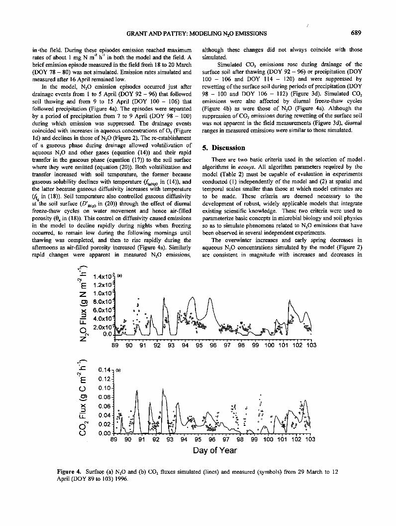
Simulated CO: emissions rose during drainage of the surface soil after thawing (DOY 92 - 96) or precipitation (DOY 100- 106 and DOY 114- 120) and were suppressed by rewetting of the surface soil during periods of precipitation (DOY 98- 100 and DOY 106- 112) (Figure 3d). Simulated CO: emissions were also affected by diurnal freeze-thaw cycles (Figure 4b) as were those of N:O (Figure 4a). Although the suppression of CO: emissions during rewetting of the surface soil was not apparent in the field measurements (Figure 3d), diurnal ranges in measured emissions were similar to those simulated.

5. Discussion

There are two basic criteria used in the selection of model,

algorithms in ecosys. All algorithm parameters required by the model (Table 2) must be capable of evaluation in experiments conducted (1) independently of the model and (2) at spatial and temporal scales smaller than those at which model estimates are to be made. These criteria are deemed necessary to the development of robust, widely applicable models that integrate existing scientific knowledge. These two criteria were used to parameterize basic concepts in microbial biology and soil physics so as to simulate phenomena related to N:O emissions that have been observed in several independent experiments.

The overwinter increases and early spring decreases in aqueous N:O concentrations simulated by the model (Figure 2) are consistent in magnitude with increases and decreases in

0 '3 1.2xl

1.0xl

,, .io l l\ 4.

0.0 •

89 90 91 92 93 94 95 96 97 98 99 100 101 102 103

0.14

012

010

0.08

0.06 0.04 0.02

o.oo

Day of Year

Figure 4. Surface (a) N:O and (b) CO: fluxes simulated (lines) and measured (symbols) from 29 March to 12 April (DOY 89 to 103) 1996.


gaseous N20 concentrations measured in frozen and thawing soils elsewhere [Burton and Beauchamp, 1994; Cares and Keeney, 1987; Flessa et al., 1995; Goodroad and Keeney, 1984; Van Bochove et al., 1996]. In the model, increases in aqueous N20 concentrations during winter follow decreases in NO3' and increases in NO2- concentrations (Figure 2), thereby reproducing the product sequence of denitrification reported by Cooper and Smith [1963]. This sequence arises from the hypothesized preference scheme for electron acceptors 0 2 > NO3'> NO2'> N20 represented in equations (4), (5) and (6) in which the reduction of acceptors with a higher oxidation number suppresses the reduction of those with a lower one.

The coupling of this preference scheme with a physically based treatment of heat and water transport through soils allowed the model to reproduce approximately the timing and intensity of N20 emissions during spring thaw (Figure 3c). These emissions were driven by C oxidation rates that were similar in magnitude to those measured (Figure 3d), indicating that the coupling of electron donors and acceptors in the model (equations (3)- (9)) was realistic. The episodic nature of N20 emissions and their association with soil thawing has also been observed by Christensen and Tiedje [1990], Flessa et al. [1995], Goodroad and Keeney [1984] and Nyborg et al. [1997]. The temporal distribution of these emissions in the model was strongly controlled by formation and melting of ice layers in the soil which impeded gas exchange with the atmosphere, as has been observed experimentally by Burton and Beauchamp [1994]. The accuracy of gaseous fluxes simulated in frozen soils therefore depends upon the extent to which the gaseous phase is reduced by ice formation. Because water migrates towards zones of freezing in ecosys, ice eventually occupies most of the non- water-filled porosity of frozen soil if enough water is present in unfrozen soil below, and so impedes gaseous transfer. The modeling work presented here thus contributes to the need indentified by Frolking et al. [1998] for models of N20 emission to simulate soil water dynamics, including freeze-thaw cycles, and to link these dynamics to denitrification activity.

The large diurnal variation of N20 emissions in the model (Figures 3c and 4a) is consistent with that measured here and elsewhere [Blackruer et al., 1982; Christensen, 1983; Robertson, 1994), and indicates the importance of temperature-sensitive hydrologic controls on these emissions. Such variation complicates efforts to make temporally integrated estimates of N20 emissions from discontinuous flux measurements. The

ability of simulation models to reproduce this variation is therefore an important test of their capability to make such estimates. It may be argued that if N20 emissions during spring thaw are driven by denitrification products accumulated under ice during the previous winter (Figure 2), then annual estimates of these emissions need only be based on estimates of total winter denitrification. However these estimates would still require a knowledge of annual freeze-thaw cycles and the kinetics of the denitrification reaction sequence, both of which may be highly variable under site-specific conditions. For example, a mid- January thaw at the field site would, according to the model, cause only small emissions of N20 (Figure 2), as has been observed elsewhere in January after several weeks of soil freezing [Christensen and Tiedje, 1990]. However, reoxygenation of the soil profile during the thaw would cause the oxidation of NO2' to NO3' [Grant, 1994], so that with the resumption of

anaerobic conditions after refreezing the reduction of NO3' to NO 2' would have to continue for some time before N20 would start to accumulate again. This delay in accumulation would cause spring emissions to be much lower than without the January thaw. Such a delay might explain the lower N20 emission rates reported from successive thawing events by Flessa et al. [1995]. Conversely a soil with more rapid rates of C oxidation than those recorded at the field site, caused perhaps by heavy fertilizer or manure applications, would generate a more intense demand for electron acceptors that under anaerobic conditions would cause the N reduction sequence to be accelerated. Such a soil would yield greater N20 emissions from a mid-winter thaw than those hypothesized here [e.g. Flessa et al., 1995], but under prolonged freezing might yield very little because the reduction sequence would be forced to completion as N 2. It therefore appears unlikely that N20 emissions can be modeled as simple functions of soil temperature or water content.

The ecosystem model ecosys simulates microbial oxidation- reduction reactions under different soil amendments such as crop residue [Grant et al., 1993a], fertilizer [Grant, 1993d; Grant, 1995] or manure, and under different soil management practices such as rotation and tillage [Grant, 1997; Grant et al., 1995; Grant and Rochette, 1994] or irrigation. By coupling these reactions to aqueous and gaseous transport of reactants and products, ecosys enables the effects of different amendments and managements on N20 emissions to be estimated. These estimates should recognize that emissions are controlled by spatial variability in substrate concentrations at two scales of resolution: (1) small scale (1 - 10 m) variability due to past C inputs and (2) larger scale (10- 100 m) variability due to topographic position (slope, aspect, elevation). The first scale is recognized to a limited extent in ecosys by calculating oxidation-reduction reactions separately for each organic substrate. For example, a small soil zone with a large concentration of easily decomposable plant residue (i = y) (often called a "hot spot") would generate a large demand for electron acceptors (R'y,h in (1)) and hence 02 (R'o2y, h in (2)). This demand, coupled to constraints imposed upon O2 transfer within the soil zone by dissolution (To2 in (14)) and diffusion (Dso in (2)) would increase the demand for

ß 2

alternative electron acceptors by denitrifiers (Re in (4)- (6)) and hence the reduction of N. The demand for electron acceptors generated by other organic substrates within the same soil zone (i ,• y) would not be affected by the demand generated by the plant residue, and the demand for alternative electron acceptors by denitrifiers would be only indirectly affected through increased competition for 02. The second scale of spatial variability is recognized in ecosys by representing landscapes as grids of north-south columns and east-west rows with defined soil

properties (e.g. Table 3) and defined slopes and aspects from which relative elevations are computed. These slopes, aspects and elevations are used in the calculation of heat, water, solute and gas fluxes in three dimensions through the simulated landscape. This representation of spatial variability has been used with the model for N20 emissions described above to demonstrate that the majority of N20 emissions from complex landscapes originate from lower slope positions (R.F. Grant, unpublished data, 1997), as has been measured experimentally. Further research at the landcape scale is needed to test ecosys and other ecosystem models in order to improve confidence in model estimates of landscape-level emissions of N20. These estimates could then be used to arrive at regional estimates of N20 emissions.


Notation •

Ags air-water interfacial area in soil (m 2 m a) (14).

D• gaseous diffusivity of gaseous substrate or product ¾ in soil (m 2 h 4) (17),(18) and (20).

D'gg¾ gaseous diffusivity of gaseous substrate or product ¾ in water at 30øC (rn 2 h 4) (t 8).

Di, h,j,c decomposition ofheterotrophs (g C m '2 h 4) (13).

ga boundary layer conductance between the atmosphere and the soil surface (h m 4) (19).

concentration of gaseous substrate or product ¾ in the atmosphere (g m '3) (19) and (20).

concentration of gaseous substrate or product ¾ in the gaseous phase of the soil (g m '3) (14), (17) and (20).

concentration of substrate or product ¾ in the aqueous phase ofthe soil (gm '3) (14), (15) and (19).

Ds% aqueous dispersivity-diffusivity of 02 in soil (m 2 h 4) (2).

M-M constant for reduction of NO2' by heterotrophic denitrifiers (g N m '3) (5).

Ds¾ aqueous dispersivity-diffusivity of substrate or product ¾ in soil (m 2 h 4) (15), (16) and (19).

KNo3d M-M constant for reduction of NO3' by heterotrophic denitrifiers (g N m '3) (4).

aqueous diffusivity of substrate or product ¾ in water at 30øC (m 2 h 4) (16).

KN2od M-M constant for reduction of N20 by heterotrophic

denitrifiers (g N m '3) (6).

volatilization-dissolution transfer coefficient (m h 4) (14).

Ko2h M-M constant for reduction of O2s by heterotrophs (g O2 m '3) (2).

am

dw

radius of heterotrophic microsite (m) (2).

radius of d m + water film at current water content (m) (2).

Fj partitioning coefficient forj in Mi, hd (13).

f• fraction of electrons not accepted by O2 transferred by denitrifiers to N oxides (3).

f• temperature function for microbial processes (dimensionless) (1).

temperature function for gaseous diffusivity (dimensionless) (18).

ftgq

•s

AGd

AGh

GM

temperature function for solubility of gaseous substrate or product ¾ (dimensionless) (14) and (19).

temperature function for aqueous diffusivity (dimensionless) (16).

water stress function for microbial processes (dimensionless) (1).

free energy change of heterotrophic C oxidation - N reduction (kJ g C 4) (12).

free energy change of heterotrophic C oxidation reduction (kJ g C 4) (12).

energy required to construct new M from Pi, k (kJ g C 4) (12)

K•

Mi, h,a

Mi, h,j,c

[NO2']

[NO;]

[N20] n

[O2m]

[O2s]

[Pi, c]

Q'gy

Q•

M-M constant for respiration of Pi, c by heterotrophs (g C m '3) (1).

hydrodynamic dispersion coefficient (m) (16). active biomass of heterotrophs (g C m '2) (1) and (2).

biomass of heterotrophs (g C m '2) (13).

concentration of NO2' in soil solution (g N m '3) (5).

concentration of NOr in soil solution (g N m '3) (4).

concentration of N20 in soil solution (g N m '3) (6). number of active heterotrophic microsites (g4) (2).

02 concentration at heterotrophic microsites (g 02 m '3) (2).

02 concentration in soil solution (g 02 m 4) (2).

concentration of soluble decomposition products of Si, c in soil solution (g C m '3) (1).

vertical transport of gaseous substrate or product ¾ between the atmosphere and the soil surface (g m '2 h 4) (2•).

vertical transport of gaseous substrate or product ¾ in the gaseous phase of the soil (g m '2 h 4) (17).

vertical transport of gaseous substrate or product ¾ between the atmosphere and the gaseous phase of the soil surface (g m '2 h 4) (20) and (21).


Q•

Qw

vertical transport of substrate or product ¾ in the aqueous phase of the soil (gm '2 h -1) (15).

vertical transport of substrate or product ¾ between the atmosphere and the aqueous phase of the soil surface (g m 4 h 'l) (19) and (21).

vertical transport of water (m 3 m '2 h -1) (15), (16) and (17).

Xs tortuosity coefficient for aqueous diffusion (16).

Ui, h,c

Uw

Dg

Pi, c uptake by Mi, h (g C m '2 h 'l) (10), (11) and (13).

root uptake of water (m 3 m '2 h 'l) (17).

sensitivity of Xg to Og (18).

sensitivity of Xs to Os (16).

0g soil air content (m 3 m '3) (18).

Op soil porosity (m 3 m '3) (18).

Os soil water content (m 3 m '3) (16).

Yd

Yh

biomass yield from heterotrophic reduction ofN (g M g C 'l) (11) and (12).

biomass yield from heterotrophic reduction of 02 (g M g C 'l) (10) and (12).

R'h

Ri, d

Ri, h

R'i,h

RMi, h

RNo2i, d

RNo3i, d

gN2oi, d

go2i, h

R'o2i, h

T¾

electron transfer to N oxides by denitrifiers (mole' m '2 h 'l) (3), (4), (5) and (6).

specific oxidation of Pi, c by heterotrophs at saturating C -1 [Pi, c], 30øC and high water potential (g C g h 'l)

oxidation of Pi, c coupled to reduction of N by denitrifiers (g C m '2 h 'l) (8), (9) and (11).

oxidation of Pi, c coupled to reduction of 02 by heterotrophs under ambient [O2s] (g C m '2 h 'l) (7), (9)- (11) and (13).

oxidation of Pi, c coupled to reduction of 02 by heterotrophs under saturating [O2s] (g C m '2 h 'l) (1) and (7).

maintenance respiration by heterotrophs (g C m '2 h -1) (10), (11) and (13).

NO2' reduction by heterotrophic denitrifiers (g N m '2 h' l) (5), (6) and (8).

NOr reduction by heterotrophic denitrifiers (g N m -2 h' l) (4), (5), (6) and (8).

N20 reduction by heterotrophic denitrifiers (g N m '2 h 'l) (6) and (8).

02 reduction by heterotrophs under ambient [O2s] (g 02 -2

m h 'l) (2), (3) and (7).

02 reduction by heterotrophs under saturating [02s] (g 02 m '2 h 'l) (2), (3) and (7).

Ostwald solubility coefficient of gaseous substrate or product ¾ at 30øC (14) and (19).

exchange of gaseous substrate or product ¾ between gaseous and aqueous phases in the soil (g m '2 h 'l) (14).

depth to mid-point of soil layer (m) (15), (17), (19) and (20).

numbers in parentheses indicate equation(s) in which variable is used.

Acknowledgements. This research is part of the Global Change and Terrestrial Ecosystems project of the International Geosphere-Biosphere Programme. It was conducted with the support of Agriculture and Agri- Food Canada, PERD program. We are grateful to Dave Dow and Mark Edwards for their excellent technical assistance.

References

Allison, F.E., S.N. Carter and L.D. Sterling, The effect of partial pressure of oxygen on alenitrification in soil, Soil Sci. Soc. Am Proc. 24, 283-285, 1960.

Ameida, J.S., M.A.M. Reis, and M.J.T. Carrondo, Competition between nitrate and nitrite reduction in denitrification by Pseudornonas fiuorescans, Biotechnol. Bioeng., 46, 476-484, 1995.

Arab, J.R.M., and A.J.A. Vinten, Simplified models of anoxia and denitrification in aggregated and simple-structured soils, Eur. J. Soil Sci., 46, 507-517, 1995.

Betlach, M.R., Accumulation of intermediates during alenitrification - Kinetic mechanisms and regulation of assimilatory nitrate uptake, Ph.D. thesis, Mich. State Univ., East Lansing, Diss. Abstr. 80:06083, 1979.

Blackmer, A.M., and J.M. Bremner, Inhibitory effect of nitrate on reduction of N20 to N 2 by soil microorganisms, Soil Biol. Blochem., 10, 187-191, 1978.

Blackmer, A.M., S.G. Robbins, and J.M. Bremner, Diurnal variability in rate of emission of nitrous oxide from soils, Soil Sci. Soc. Am. J., 46, 937-942, 1982.

Bremner, J.M., and K. Shaw, Denitrification in soils, II, Factors affecting denitrification, J. Agric. Sci., 51, 40-52, 1958.

Bresler, E., Simultaneous transport of solutes and water under transient unsaturated flow conditions, Water Resour. Res., 9, 975-986, 1973.

Burton, D.L.. and E.G. Beauchamp, Profile nitrous oxide and carbon dioxide concentrations in a soil subject to freezing. Soil Sci. Soc. Am. J., 58, 116-122, 1994.


Cady, F.B., and W.V. Bartholomew, Influence of low pO2 on denitrification processes and products, Soil Sci. Soc. Am. Proc., 25, 362-365, 1961.

Campbell, G.S., Soil Physics with BASIC, 185 pp., Elsevier, New York, 1985.

Cares, R.L.,Jr., and D.R. Keeney, Nitrous oxide production throughout the year from fertilized and manured maize fields, J. Environ. Qual., 16, 443-447, 1987.

Christensen, S., Nitrous oxide emission from a soil tinder permanent grass: seasonal and diurnal fluctuations as influenced by manuring and fertilization, Soil Biol. Blochem., 15,.531-536, 1983.

Christensen, S., and J.M. Tiedje, Brief and vigorous N20 production by soil at spring thaw, o r. Soil Sci., 41, 1-4, 1990.

Cooper, G.S., and R.L. Smith, Sequence of products formed during denitrification in some diverse western soils, Soil Sci. Soc. Am. Proc., 27, 659-662, 1963.

Elliott, R.G., and C.M. Gilmour, Growth of Pseudomonas stutzeri with nitrate and oxygen as terminal electron acceptors, Soil Biol. Biochem., 3, 331-335, 1971.

Firestone, M.K., M.S. Smith, R.B. Firestone, and J.M. Tiedje, The influence of nitrate, nitrite and oxygen on the composition of the gaseous products of denitrification in soil, Soil Sci. Soc. Am. J., 43, 1140-1144, 1979.

Flessa, H., P. D6rsch, and F. Beese, Seasonal variation of N20 and CH 4 fluxes in differently managed arable soils in southern Germany, J. Geophys. Res., 100, 23115-23124, 1995.

Frolking, S.E., et al., Comparison of N20 emissions from soils at three temperate agricultural sites: simulations of year-round measurements by four models, Nutr. Cycling. Agroecosyst., in press, 1998.

Goodroad, L.L., and D.R. Keeney, Nitrous oxide emissions from soils during thawing, Can. J. Soil Sci., 64, 187-194, 1984.

Grant, R.F., Dynamic simulation of phase changes in snowpacks and soils, Soil Sci. Soc. Am. J., 56, 1051-1062, 1992.

Grant, R.F., Simulation of ecological controls on nitrification, Soil Biol. Blochem., 26, 305-315, 1994.

Grant, R.F., Mathematical modelling of nitrous oxide evolution during nitrification, Soil Biol. Blochem., 27, 1117-1125, 1995.

Grant, R.F., ecosys. Global Change and Terrestrial Ecosystems Task 3.3.1 Soil Organic Matter Network (SOMNED: 1996 Model and Experimental Metadata., pp. 19-24, Nat. Environ. Res. Counc. Cent. for Ecol. and Hydrol., Wallingford, Oxon, England, 1996.

Grant, R.F., Changes in soil organic matter under different tillage and rotation: Mathematical modelling in ecosys, Soil Sci. Soc. Am. J., 61, 752-764, 1997.

Grant, R.F., Mathematical modelling of methanogenesis in ecosys, Soil Biol. Biochem., 30, 883-896, 1998.

Grant, R.F., Mathematical modelling of methanotrophy in ecosys, Soil Biol. Blochem., 31: 287-297, 1999.

Grant, R.F., and P. Rochette, Soil microbial respiration at different temperatures and water potentials: Theory and mathematical modelling, Soil Sci. Soc Am. J., 58, 1681-1690, 1994.

Grant, R.F., R.C. Izaurralde, and D.S. Chanasyk, Soil temperature under different surface managements: testing a simulation model, Agric. For. Meteorol., 73, 89-113, 1995.

Grant, R.F., N.G. Juma, and W.B. McGill, Simulation of carbon and nitrogen transformations in soils, I, Mineralization, Soil Biol. Biochem., 27, 1317-1329, 1993a.

Grant, R.F., N.G. Juma, and W.B. McGill, Simulation of carbon and nitrogen transformations in soils, II, Microbial biomass and metabolic products, Soil Biol. Biochem., 27, 1331-1338, 1993b.

Grant, R.F., M. Nyborg, and J. Laidlaw, Evolution of nitrous oxide.from soil, I, Model development, Soil Sci., 156, 259- 265, 1993c.

Grant, R.F., M. Nyborg, and J. Laidlaw, Evolution of nitrous oxide from soil, II, Experimental results and model testing, Soil Sci., 156, 266-277, 1993d.

Griffin, D.M., Ecology of Soil Fungi, 193 pp., Syracuse Univ. Press, Syracuse N.Y., 1972.

Horst, T.W., and J.C. Weil, How far is far enough? The fetch requirements for micrometeorological measurement of surface fluxes, J. Atmos. Oceanic Technol., 11, 1018-1025, 1994.

Kemper, W.D., and J.B. Rollins, Osmotic efficiency coefficients across compacted clays, Soil Sci. Soc. Amer. Proc., 30, 529- 534, 1966.

Koike, I., and A. Hattori, Growth yield of a denitrifying bacterium, Pseudomonas denitrificans, under aerobic and denitrifying conditions, J. Gen. Microbiol., 88, 1-10, 1975a.

Koike, I., and A. Hattori, Energy yield of denitrification: An estimate from growth yield in continuous cultures of Pseudomonas denitrificans under nitrate-, nitrite- and nitrous oxide-limited conditions, J. Gen. Microbiol., 88, 11-19, 1975b.

Leffelaar, P.A., and W.W. Wessel, Denitrification in a homogeneous, closed system: experiment and simulation, Soil Sci., 146, 335-349, 1988.

Li, C., S. Frolking, and T.A. Frolking, A model of nitrous oxide evolution driven by rainfall events, I, Model structure and sensitivity, J. Geophys. Res., 97, 9759-9776, 1992.

McConnaughey, P.K., and D.R. Bouldin, Transient microsite models of denitrification, I, Model development, Soil Sci. Soc. Am. J., 49, 886-891, 1985.

McGill, W.B., H.W. Hunt, R.G.Woodmansee, and J.O. Reuss, Phoenix, a model of the dynamics of carbon and nitrogen in grassland soils, in Terrestrial Nitrogen Cycles, edited by F.E. Clark and T. Rosswall, Ecol. Bull., 33, 49-115, 1981.

Millington, R.J., Gas difusion in porous media, Science, 130, 100-102, 1959.

Nommik, H. Investigations on denitrification, Acta Agric. Scand., 6, 195-228, 1956.

Nyborg, M., J.W. Laidlaw, E.D. Solberg, and S.S. Malhi, Denitrification and nitrous oxide emissions from a Black

Chernozemic soil during Spring thaw in Alberta, Can. J. Soil Sci., 77, 153-160, 1997.

Ogram, G.L., F.J. Northrup, and G.C. Edwards, Fast time response tunable diode laser measurements of atmospheric trace gases for eddy correlation, J. Atto. Oceanic Tech., 5(4), 521-527, 1988.

Parton, W.J., A.R. Mosier, D.S. Ojima, D.W. Valentine, D.S. Schimel, K. Weier, and A.E. Kulmala, Generalized model for N2 and N20 production from nitrification and denitrification, Global Biogeochem. Cycles, 10, 401-412, 1996.

Pattey, E., W.G. Royds, R.L. Desjardins, D.J. Buckley, and P.


Rochette, Software description of a data acquisition and control system for measuring trace gas and energy fluxes by eddy-accumulation and correlation techniques, Cornput. Electron. Agric., 15(4), 303-321, 1996.

Paulson, C.A., The mathematical representation of wind speed and profile temperatures in the unstable atmospheric surface layer, J. Appl. Meteorol., 9, 857-861, 1970.

Pirt, S.J., Principles of Microbe and Cell Cultivation, 274 pp., Blackwell Sci., Cambridge, Mass, 1975.

Ridge, E.H., Studies on soil fumigation, II, Effects on bacteria, Soil Biol. Biochem., 8, 249-253, 1976.

Robertson, K., Nitrous oxide emission in relation to soil factors at low to intermediate moisture levels, J. Environ. Qual., 23, 805-809, 1994.

Shields, J.A., E.A. Paul, and W.E. Lowe, Factors influencing the stability of labelled microbial materials in soils. Soil Biol. Biochern., 6, 31-37, 1974.

Simpson, I.J., G.W. Thurtell, H.H. Neumann, G. den Hartog, and G.C. Edwards, The validity of similarity theory in the roughness sublayer above forests. Boundary Layer Meteorol., in press, 1998.

Skopp J., Oxygen uptake and transfer in soils: analysis of the air- water interfacial area, Soil Sci. Soc Am. J., 49, 1327-1331, 1985.

Smid, A.E., and E.G. Beauchamp, Effects of temperature and organic matter on denitrification in soil, Can. J. Soil Sci., 56, 385-391, 1976.

Van Bochove, E., H.G. Jones, F. Pelletier, and D. Pr6vost, Emission of N20 from agricultural soil under snow cover: a

significant part of N budget, Hydrol. Proc., 10, 1545-1549, 1996.

Wagner-Riddle, C., G.W. Thurtell, G.E. Kidd, G.C. Edwards, and I.J. Simpson, Micometeorological measurements of trace gas fluxes from agricultural and natural ecosystems, InJ?ared Phys. Technol. 37, 51-58. 1996,

Weier, K.L., J.W. Doran, J.F. Power, and D.T. Walters, Denitrification and the dinitrogen/nitrous oxide ratio as affected by soil water, available C and nitrate, Soil Sci. Soc. Am. J., 57, 66-72, 1993.

.

Wienhold, F.G., H. Frahm, and G.W. Harris, Measurements of N20 fluxes from fertilized grassland using a fast response tunable diode laser spectrometer, J. Geophys. Res., 99, 16557-16567, 1994.

Wilhelm, E., R. Battino, and R.J. Wilcock, Low-pressure solubility of gases in liquid water, Chern. Rev., 77, 219-262, 1977.

Yoshinari, T., R. Hynes, and R. Knowles, Acetylene inhibition of nitrous oxide reduction and measurement of denitrification

and nitrogen fixation in soil, Soil Biol. Blochem., 9, 177-183, 1977.

R. Grant, Department of Renewable Resources, University of Alberta, 442 Earth Sciences Building, Edmonton, Alberta, T6G 2H1, Canada. (robert.grant•ualberta. ca)

(Received May 20, 1998; revised October 19, 1998; accepted November 17, 1998.)

Mathematical modeling of nitrous oxide emissions from … · GLOBAL BIOGEOCHEMICAL CYCLES, VOL. 13,...

Documents

Transcript of Mathematical modeling of nitrous oxide emissions from … · GLOBAL BIOGEOCHEMICAL CYCLES, VOL. 13,...