Mathematical modeling of fluid flow using the numerical scheme with artificial viscosity

Ing. Tomáš Sommer, Ing. Martin Helmich

Thesis supervised by: Doc. Svatomír Slavík, CSc., Doc. Luboš Janko, CSc.

Abstract

This paper deals with mathematical modeling and numerical solution of hyperbolic partial differential equations with verification of the inviscid compressible fluid. The solution flow is used finite volume method defined on a structured quadrilateral computational mesh. Outcome of this work is to create a custom program solver in the calculation of Matlab. As a test example was chosen planar channel having a concave bottom portion. Research results are compared with the works of other authors published in the literature and commercial software. Key words

FVM; structured mesh; quadrilateral grid; subsonic; transonic; supersonic; MacCormack scheme; Jameson´s artificial viscosity;TVD; Causon´s simplified; Euler equations

1. The mathematical model of compressible inviscid fluid

Numerical solution of compressible inviscid fluid is described non-linear conservative system of the Euler equations, which are a special case of Navier-Stokes equations. It can be shown that the system of Euler equations is hyperbolic.

1.1. Basic equations of fluid dynamics

Conservative system of the Euler equations representing the mathematical model of compressible inviscid and thermally non-conductive fluid, generally based on the laws of conservation of mass, conservation of momentum - the two equilibrium equations of forces (2D) and the law of conservation of energy. This work deals with dvoudimenzionálním compressible inviscid fluid flow, therefore the system of Euler equations in matrix notation:

Shorthand notation: 1.2. The constitutive relations

Because of the conservative system has more unknowns than equations, it must be add the thermal equation of state showing the relationship between status variables. Compressible gas is often thought of as an ideal gas, the following applies:

Furthermore, the compressible fluid is characterized by the speed of sound, wherein the propagation of sound in an ideal gas can be considered as the adiabatic process, respectively. isentropic - changes occur rapidly, so that there is no exchange of heat with the surroundings.

Local flow state is characterized by a Mach number:

The constitutive relation for the pressure, expressed in terms of the conservative variables:

2. Numerical solutions of the Euler equations

2.1. Finite Volume Method The finite volume method (FVM) was established theory at the beginning of the seventies, but wider use recorded in the eighties. It is used in approximately 80% of commercial programs. Computing solutions area is divided into a finite number of small non-overlapping control volumes over the grid. For each control volume, then apply the system of equations separately. FVM uses the integral form of equations, the basic equations describing the continuum are disktetizovány into a system of algebraic equations. The values of the searched velocity components and scalar variables are stored in the geometric centers of control volumes, values at the border volumes are obtained by interpolation. In our case, flow through the control volume boundary in 2D is integral sums over the four faces of the control volume. Length side of the cell control volume:

The normal vector to the side of the control volume:

Unit the outer normal vector:

The contents of quadrangular volume:

Fig. 1 – Control volume with the computational point P and nodes

2.2. MacCormack scheme The scheme was originally developed for the method of finite differences. Today can be successfully used to solve both the Euler and the Navier-Stokes equations. Although present age has been replaced by more efficient and faster switching. For its simplicity and reliability are among the classical scheme, among the representatives of the schemes of second order accuracy. The scheme has satisfactory accuracy achieved good results both in the flow subject to strong shock waves are at unsteady flow, but the flow is compared with the viscosity of the newer schemes slow. The disadvantage of scheme as well as in other schemes of higher order of accuracy is dispersive defect, which causes oscillations in the solution, which in the nonlinear case, lead to loss of stability. Therefore, it is always necessary to add the scheme member with artificial viscosity that dampens ocsilace. MacCormackovo scheme is a two-step method, second order accuracy. Higher order interpolation schemes are generally more accurate but less stable with a longer computing time. This is basically the Lax-Wendroffovo scheme written in the form predictor-collector. It uses the auxiliary values between time layers, which in turn will use to obtain new values of the unknown function at time tn+1 layer. 2.3. Convergence and stability Explicit scheme works as gradual process, where the convergence is expressed by means of residues selected variable Z.

The stability of difference schemes can be done in several ways, in our case we use spectral analysis, the determination of residues is using discrete L2 norms of the time derivative of the density of the individual components of speed and power based on the content of each control volume. The value Δt indicates the time step size, representing a necessary condition, but not sufficient to guarantee the stability and convergence of the calculation. Time step sizes also affects the size of the grid, speed in the computational domain and the selected value of the constant CFL from the interval (0,1).

Where:

a the maximum absolute value of the eigenvalues of the Jacobian matrix

and a lengths are approximations of the control volume in the direction of i and j

2.4. MacCormack scheme with artificial viscosity type Jameson

This chapter outlines the creation of a two-step explicit numerical solution scheme MacCormackova finite volume method on structured quadrilateral network, specifically in the variant with artificial viscosity Jamesového type. The scheme is in the form of a predictor - corrector.

For capturing the smoothed shock waves and prevent instability in the form of oscillations is necessary to add a schema damping member with artificial viscosity. In the case of James damping parameters are unknown and depends on the specific solution calculation.

Search the numerical solution at the time tn +1 are fixed damping member with artificial

viscosity: Where damping members are:

Similarly, to derive the equation for the direction j. The values of the speed of the walls of the control cells dealt zone can be expressed as the arithmetic average of the values of two adjacent cells:

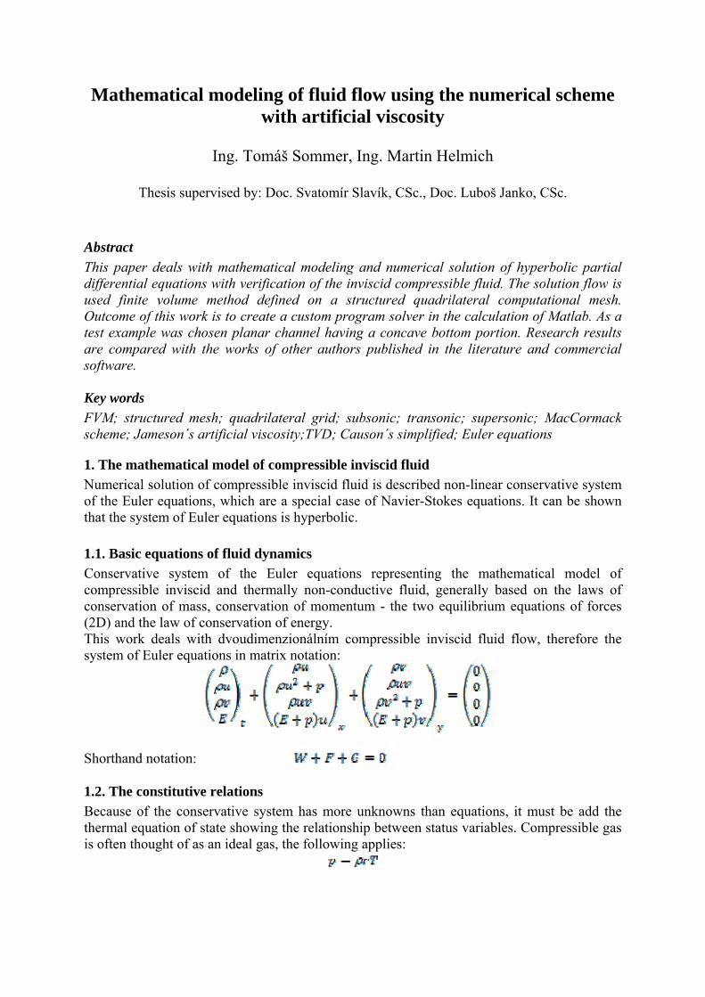
2.5. TVD MacCormack scheme in Causon's simplified

As already mentioned in Chapter 2.2 difference scheme type Lax-Wendroff second order accuracy near discontinuities, such as shock waves produce strong oscillations leading to numerical instability of the solution. Therefore, at the beginning of the 80th twentieth century began to appear TVD schemes designed to solve problems with discontinuities such as shock waves. The design scheme consists in adding damping members TVD - and without introducing unknown parameters as in the previous case. Damping member add to MacCormack scheme after corector step, so that will corrector the numerical solution in time tn+1:

Where damping members are defined by the following relations:

For apply:

The function: Limiter:

Courant number:

2.6. The boundary conditions for the system of Euler equations

Number of prescribed boundary conditions of inlet and outlet is determined by the number of positive and negative eigenvalues in solving the Jacobian matrices of inviscid fluxes vector when their number varies with the type of flow.

The boundary condition inlet For subsonic flow type specifying three variables and other variables extrapolated from the flow field. Specifically, in our case, the parameters of flow p0, ρ0, and the angle of attack α.

In the case of supersonic inlet is necessary to prescribe all four variables. In our case it is ρ1, M1, u1 and v1.

The boundary condition outlet

In the case of subsonic outlet fluid exits from the area of computational environment to a known pressure pout. The flow field is extrapolated first three components of the vector of

conservative variables. The fourth component of the vector W - energy, we calculate by:

In the case of supersonic outlet should be all variables to determine the extrapolation of the flow field.

Wall boundary condition In our case it is the idealized model inviscid walls, without a boundary layer and velocity profile. The pressure on the wall of replacing the pressure in the nearest cell adjacent to the wall. Condition impermeability of the wall:

3. Application of numerical solution Pro ověření správnosti, funkčnosti a vhodnosti vytvořeného vlastního programu ve výpočtovém prostředí Matlab a pro zvolené numerické řešení použitých schémat byla vybrána testovací úlohu rovinný kanál s vydutou částí na spodní straně - Ron-Ho-Ni kanál, resp. takzvaný GAMM kanál.

Dimensions of the control volume are x ∈ <0, 3>, y ∈ <0, 1>. For supersonic flow with the creation of a system of shock waves were calculated area extended by one part arc x ∈ <0, 4>, y ∈ <0, 1>. The middle bottom is found 10% of the profile-arc lying in the area x ∈ <1, 2>, y ∈ <0, 0,1>. 3.1. Discretization of the computational region To verify correctness functionality and suitability program developed in Matlab computational environment and selected for the numerical solution of the schemes was selected test example planar channel with a concave portion on the bottom – Ron-Ho-Ni channel, respectively GAMM channel. Two-dimensional computational limited area represented by the mentioned channels is bounded by four boundaries:

Inlet (x=0) - part of the boundary, which flow enters into the computational domain Outlet (x=3, respectively 4) - part of the boundary, which stream is output from

computational domain The bottom wall (y = 0) - solid impervious wall with a concave arc The upper wall (y = 1) - solid impervious wall

For specific test case numerical simulations were used three types of networks, specifically for the case of subsonic flow of 150x50 grid cells, in case of mesh testing transonic flow of 231x50 cells and finally in the case of a supersonic flow of 321x80 grid cells. When calculating the subsonic flow was used uniform quadrilateral grid.

Fig. 2 – Structured quadrilateral computational grid of 150 x 50 cells for inviscid subsonic flow

Fig. 3 – Structured quadrilateral computational grid of 231 x 50 cells for inviscid transonic flow

When calculating transonic flow was used not uniform quadrilateral mesh, densified in the second and third part of the block, which is expected incidence of shock waves. When calculating the supersonic flow of the control volume at the end of one extended portion of the chord width of arcs.

Fig. 4 – Structured quadrilateral computational grid of 321 x 80 cells for inviscid supersonic flow 3.2. The results of numerical solutions for subsonic flow In solving subsonic flow we consider subsonic input and output, and prescribe the three input variables and one outlet. The remaining values are interpolated from the computational domain. In our case, the subsonic flow of a fluid characterized by the value of the Mach number M = 0.5:

pO=120196 [Pa] ρO=1,3297 [kg.m-3] α=0 [°]

pout=101325 [Pa] CFL=0,7 James damping constants α2=0,8 [-], α4= 0,035[-]

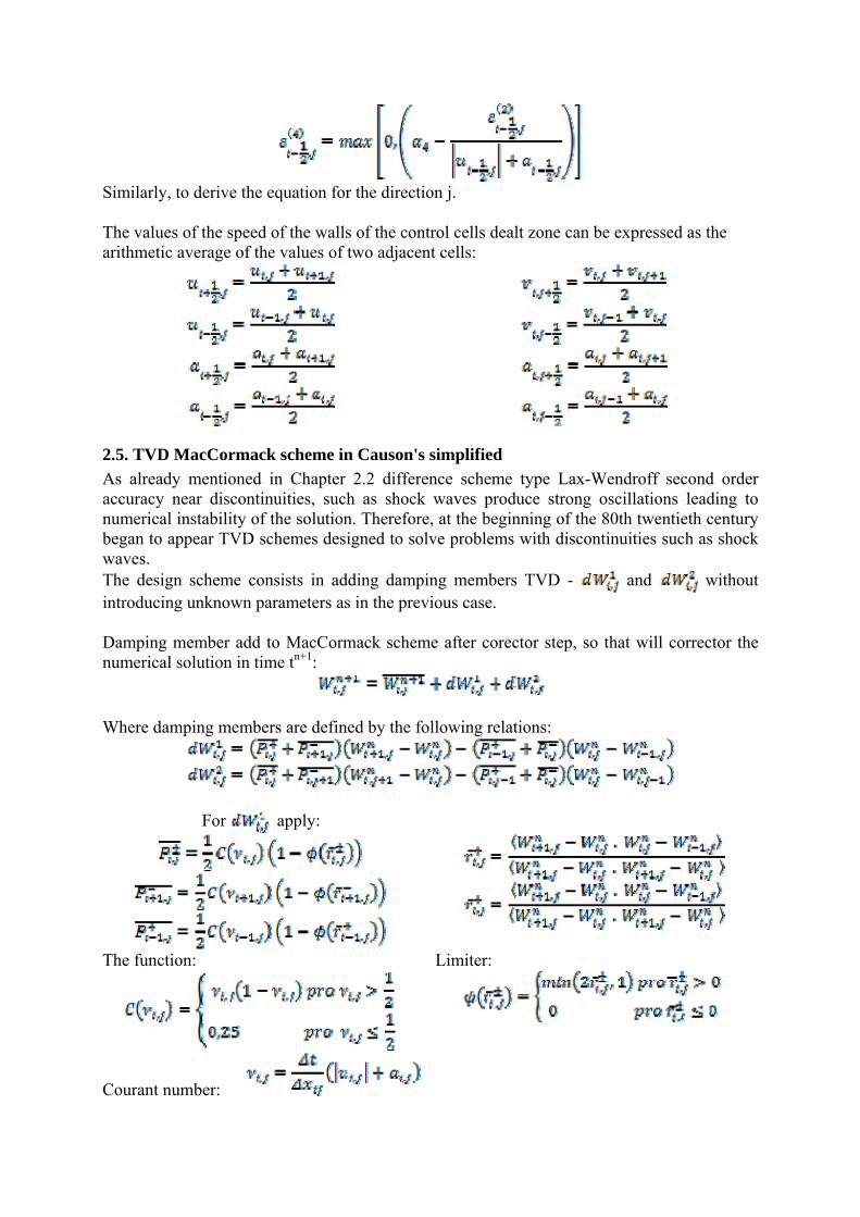
On Fig. 6 shows the results - isolines of the Mach number in the investigated area in Fig. 5 show similar outcomes static pressure. Individual results are in good agreement with those reported in the literature [1, 6].

Fig. 5 – The distribution of static pressure in the GAMM channel for subsonic inviscid flow [Pa] - Jameson

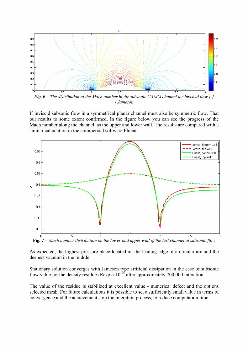
Fig. 6 – The distribution of the Mach number in the subsonic GAMM channel for inviscid flow [-] - Jameson

If inviscid subsonic flow in a symmetrical planar channel must also be symmetric flow. That our results to some extent confirmed. In the figure below you can see the progress of the Mach number along the channel, as the upper and lower wall. The results are compared with a similar calculation in the commercial software Fluent.

Fig. 7 – Mach number distribution on the lower and upper wall of the test channel at subsonic flow As expected, the highest pressure place located on the leading edge of a circular arc and the deepest vacuum in the middle. Stationary solution converges with Jameson type artificial dissipation in the case of subsonic flow value for the density residues Rezρ ≈ 10-25 after approximately 700,000 interation. The value of the residue is stabilized at excellent value - numerical defect and the options selected mesh. For future calculations it is possible to set a sufficiently small value in terms of convergence and the achievement stop the interation process, to reduce computation time.

Fig. 8 – Convergence for subsonic flow on structured quadrilateral mesh of 150 x 50 cells - Jameson

3.3. The results of numerical solutions for transonic flow As a second example of numerical solution of compressible inviscid fluid in internal aerodynamics using the finite volume method is transonic flow in the same channel with identical geometry. This task is already foreseen occurrence of supersonic areas, therefore the mesh is smoothed. In transonic flow is considered subsonic inlet and outlet, and prescribe the three inlet variables to outlet one. The remaining values are interpolated from the computational domain.

In our case we choose subsonic fluid flow characterized by the value of the Mach number M = 0.675:

pO=137483 [Pa] ρO=1,4637 [kg.m-3] α=0 [°]

pout=101325 [Pa] CFL=0,7 James damping constants α2=0,75 [-], α4= 0,02[-]

It is assumed that at transonic inviscid flow does not occur in the channel losses, the outlet pressure is chosen the same as the input. Losses in the shock wave of low intensity can be neglected.

Fig. 9 – The distribution of static pressure in the GAMM channel for transonic inviscid flow [Pa] - Jameson

Mesh in the above profile is softened due to the expected shock wave formation in the second half of the arc. This assumption proved to be correct and the other images distribution of static pressure and Mach number in the test channel is clearly visible small region of supersonic flow finished a shock wave.

Fig. 10 – The distribution of the Mach number in the transonic GAMM channel for inviscid flow [-] - Jameson

Transonic flow was next to the numerical solution of the MacCormack scheme with Jameson´s artificial viscosity used and modified TVD scheme in MacCormackovo Causon 's simplified. Results obtained modified TVD scheme again expressed isolines static pressure and Mach number are shown below.

Fig. 11 – The distribution of static pressure in the GAMM channel for transonic inviscid flow [Pa] - TVD (Causon 's simplified)

Fig. 12 – The distribution of the Mach number in the transonic GAMM channel for inviscid flow [-] - TVD (Causon 's simplified)

It is a well-known test example, when the available literature and numerical analysis is provided that the maximum Mach number in the calculation should reach values of 1.37 to 1.4. The Fig. 13, it can be seen that in the case of calculation using MacCormackova scheme

with artificial viscosity James's type (red) is on the bottom wall in the second half of the arc achieved Mmax ≈ 1.398 [-]. If MacCormackova TVD scheme in Causon 's simplified (blue) is reached Mmax ≈ 1.42 [-] and in the case of using a commercial solver Fluent (green) Mmax ≈ 1.38 [-].

Fig. 13 – Mach number distribution on the lower and upper wall of the test channel at transonic flowFurthermore, it is known that a shock wave should detect next local maximum Mach number, known under the designation Zierepova singularity. The convergence is seen that the stationary solution is achieved by the scheme with artificial viscosity type Jameson in the case of transonic flow for the value of the residue density Rezρ ≈ 10-23 after approximately 180,000 interation.

Fig. 14 – Convergence for transonic flow on structured quadrilateral mesh of 231 x 50 cells 3.4 The results of the numerical solution for supersonic flow For supersonic flow we assume inlet and outlet supersonic and prescribes the four input variables, the outlet no. The remaining values are interpolated from the computational domain.

In our case we choose supersonic fluid flow characterized by: Minl=1,65 uinl=572,866 [m.s-1] vinl=0 [m.s-1]

ρinl=1,177 [kg.m-3] CFL=0,5 James damping constants α2=0,95 [-], α4= 0,02[-]

Results supersonic flow obtained using the schema again with James's damping are shown below - isolines of static pressure, Mach number.

Fig. 15 – The distribution of static pressure in the GAMM channel for supersonic inviscid flow [Pa] - Jameson

Fig. 16 – The distribution of the Mach number in the supersonic GAMM channel for inviscid flow [-] - Jameson

Individual results are in very good agreement with the results in [1, 6]. The Fig. 17 is clearly visible layout Mach numbers the upper and lower wall of the channel. Different results compared with those obtained by the commercial software Fluent (green) in the second half of the channel is caused by the different order of solutions. The results from Fluent are first order - the calculation was stable but less accurate (continuous smooth).

Fig. 17 – Mach number distribution on the lower and upper wall of the test channel at supersonic flow

Fig. 18 – Convergence for supersonic flow on struct. quadrilateral mesh of 321 x 80 cell - Jameson The convergence is seen that the stationary solution is achieved by the scheme with artificial viscosity type Jameson in the case of supersonic flow for the value of the residue density Rezρ ≈ 10-23 after approximately 60,000 interation. 4. Numerical simulation in Fluent For comparison, the jobs were also solved by commercial software - Fluent 6.3 Due to the compressible solution was included in the calculation equation of energy. As a model changes in air density due to compressibility was set to the ideal gas law. The network was chosen identical - a quadrilateral mesh of cells, as in the case of own software. As a numerical calculation scheme was chosen chart type upwind second or first order. Schema type for upwind finite volume method can be written in the form [2]:

Value Courantova CFL numbers, indicating the relationship between the time and space step was allowed at the default value. The value affects the stability of the solution. 5. Conclusion - Analysis and comparison of results The numerical solution of nonlinear hyperbolic system Euler equations were performed using one to two variants of a two-step scheme MacCormackova the structured quadrilateral grid. Specifically, subsonic and supersonic flow was solved using the MacCormack scheme with Jameson artificial viscosity type. In the case of transonic flow control Jameson was next used and modified TVD scheme in MacCormackovo Causon 's simplified. All these variants flow were compared with those obtained from commercially available solvers for CFD calculations - Fluent.

To assess the quality of the numerical solution can be used as determining the maximum value of the Mach number on the bottom wall of the channel, localization and quality rendering Zierepovy singularity and overall quality differentiation shock waves. In the case of subsonic and supersonic flow of the individual results are in good agreement with those reported in the literature [1, 6]. It is also achieved good agreement with the results of a commercial solver. Only in the case of supersonic flow (Fig. 17), there are differences in the second half of the channel solved using commercial software, which was used in the calculation of stable first-order accuracy. It is obvious that if we apply the method of second order accuracy, the step change, large gradient magnitudes for the shockwave displayed sharp enough. The results obtained during the transonic flow can be gradual process of convergence displayed in the Fig. 13 to evaluate the two selected numerical schemes achieve similar levels of residues, but modified TVD scheme converges to the stationary solution of 48% faster, is approximately twice faster. In contrast, the variant with Jamesovovým damping achieves relatively sharp capture Zierepovy singularity, maximum value of the Mach number is within the specified limits (Mmax = 1.398). Results obtained by a modified TVD scheme are almost identical, but less damped Mmax = 1.42 and is less determined area of the second local maximum Mach number. The performed numerical tests can be seen that using a two-step scheme MacCormackova artificial dissipation can be used for all types of flow, and gives very good results with all types of flow. MacCormackovo modified TVD scheme in Causon 's simplified gives almost identical results and achieved satisfactory results in the test transonic flow. On the other hand, a strong disadvantage James damping control are unknown constants α2 and α4, which is necessary for every computing task and a mesh of experimentally determined. This disadvantage of the modified TVD scheme is omitted. Symbols a speed of sound [m/s] A, B Jacobi matrix [-] C constant TVD scheme [-] dW damping member in the individual Schemes [kg.m-3, kg.m-1.s-2,

kg.m-1.s-2, kg.m-2.s-2] E total energy per unit volume [J] F, G inviscid fluxes vector [kg.m-2.s-1, kg.m-1.s-

2, kg.m-1.s-2, kg.s-3]

l length side of the cell [m] M Mach number [-] n unit the outer normal vector [-] N normal vector having the direction of the outer normal unit

vector n [-]

p static pressure [Pa] p0 stagnation pressure [Pa] r specific gas constant [J.kg-1.K-1] T temperature [K]

u, v cartesian components of the velocity vector [m/s] V total velocity vector [m/s] W vector of conservative variables [kg.m-3, kg.m-1.s-2,

kg.m-1.s-2, kg.m-2.s-2] x, y cartesian components of the vector of spatial coordinates [-] angle of attack [°] 2, 4 constant artificial viscosity Jameson type [-] Δt time step of the numerical scheme [s] Δx, Δy steps in the direction of the coordinates x, y [m] φ flux limiter in the TVD scheme [-] λi i-th inherent number [-] κ Poisson adiabatic constant [-] ν Courant number [-] Ωij volume control mesh [m2] density [km.m-3] 0 stagnation density [km.m-3] List of abbreviations

2D two-dimensional CFD Computational Fluid Dynamics CFL Courant–Friedrichs–Lewy (condition) FVM Finite Volume Method TVD Total Variation Diminishing References

[1] VIMMR, J.: Matematické modelování proudění stlačitelné tekutiny ve vnitření aerodynamice. Disertační práce. Plzeň 2002

[2] DVOŘÁK, R.; KOZEL, K.: J.: Matematické modelování v aerodynamice, ČVUT, Praha 1996

[3] FÜRST, J.: Numerical Solution of Compressible Flows Using TVD and ENO Finite Volume Methods, Habilitation, Praha 2004

[4] KOZEL, K.: Numerické metody řešení problémů proudění I., II. Praha: ČVUT, 2001. [5] ESFAHANIAN, V.; AKBARZADEN, P.: The Jameson’s numerical method for

solving the incompressible viscous and inviscid flows by means of artificial compressibility and preconditioning method, Applied Mathematics and Computation, Volume 206, Issue 2, 15 December 2008, Pages 651–661

[6] FERZIGER, J.H.; PÉRIĆ, M..: Computational Methods for Fluid Dynamics, Springer-Verlag, Berlin, Heidelberg, 1999

[7] ANDERSON, D. A.: Computational Fluid Mechanics and Heat Transfer, Hemisphere Publishing Corporation, New York, 1984

[8] HIRSCH, C.: Numerical Computation of Internal and External Flows, John Wiley & Sons, 1990