Mathematical Modeling of Biofilms Abstract Isbn1843390876 Contents

8/14/2019 Mathematical Modeling of Biofilms Abstract Isbn1843390876 Contents

http://slidepdf.com/reader/full/mathematical-modeling-of-biofilms-abstract-isbn1843390876-contents 1/18

Scientific and Technical Report No.18

Mathematical Modeling of Biofilms

IWA Task Group on Biofilm Modeling:Hermann Eberl, Eberhard Morgenroth,

Daniel Noguera, Cristian Picioreanu,Bruce Rittmann, Mark van Loosdrechtand Oskar Wanner



Published by IWA Publishing, Alliance House, 12 Caxton Street, London SW1H 0QS, UK

Telephone: +44 (0) 20 7654 5500; Fax: +44 (0) 20 7654 5555; Email: [email protected]

Web: www.iwapublishing.com

First published 2006

© 2006 IWA Publishing

Index prepared by Indexing Specialists, Hove, UK.

Printed by Lightning Source

Apart from any fair dealing for the purposes of research or private study, or criticism or review, as permitted under

the UK Copyright, Designs and Patents Act (1998), no part of this publication may be reproduced, stored or

transmitted in any form or by any means, without the prior permission in writing of the publisher, or, in the case of

photographic reproduction, in accordance with the terms of licences issued by the Copyright Licensing Agency in

the UK, or in accordance with the terms of licenses issued by the appropriate reproduction rights organization

outside the UK. Enquiries concerning reproduction outside the terms stated here should be sent to IWA Publishing

at the address printed above.

The publisher makes no representation, express or implied, with regard to the accuracy of the information contained

in this book and cannot accept any legal responsibility or liability for errors or omissions that may be made.

Disclaimer

The information provided and the opinions given in this publication are not necessarily those of IWA or of the authors,

and should not be acted upon without independent consideration and professional advice. IWA and the authors will not

accept responsibility for any loss or damage suffered by any person acting or refraining from acting upon any material

contained in this publication.

British Library Cataloguing in Publication Data

A CIP catalogue record for this book is available from the British Library

Library of Congress Cataloging- in-Publication Data

A catalog record for this book is available from the Library of Congress

ISBN 1843390876

ISBN13: 9781843390879



Contents

LIST OF TASK GROUP MEMBERS ...........................................................................................ix

ACKNOWLEDGEMENTS .............................................................................................................x

OVERVIEW ....................................................................................................................................xi

1. INTRODUCTION … ............................. .............................. .............................. ..........................1

1.1 WHAT IS A BIOFILM? .............................. ............................... ................................ .............1

1.2 GOOD AND BAD BIOFILMS................................................................................................2

1.3 WHAT IS A MODEL? ............................ ............................... .............................. ...................4

1.4 THE RESEARCH CONTEXT FOR BIOFILM MODELING.................................................5

1.5 A BRIEF OVERVIEW OF BIOFILM MODELS....................................................................6

1.6 GOALS FOR BIOFILM MODELING ............................. ................................ .......................7

1.7 THE IWA TASK GROUP ON BIOFILM MODELING............................ .............................8

1.8 OVERVIEW OF THIS REPORT ............................... ................................ .............................8

1.8.1 Guidance for model selection........................................................................................8

1.8.2 Biofilm models considered by the Task Group ........................... ............................ ......9

1.8.3 Benchmark problems...................................................................................................10

2. MODEL SELECTION ..........................................................................................................….11

2.1 BIOFILM FEATURES RELEVANT TO MODELING ........................... .............................11

2.2 COMPARTMENTS...............................................................................................................12

2.2.1 The biofilm..................................................................................................................12

2.2.2 The bulk liquid .............................. ............................... .............................. .................15

2.2.3 The mass-transfer boundary layer ............................ ............................. ......................16

2.2.4 The substratum............................................................................................................17

2.2.5 The gas phase ............................ ............................... .............................. .....................17



vi Mathematical modeling of biofilms

2.3 COMPONENTS.....................................................................................................................17

2.3.1 Dissolved components.................................................................................................17

2.3.2 Particulate components................................................................................................20

2.4 PROCESSES AND MASS BALANCES...............................................................................21

2.4.1 Transformation processes............................................................................................22

2.4.2 Transport processes.............................. .............................. .............................. ...........25

2.4.3 Transfer processes................................ ............................... ................................ ........262.5 MODEL PARAMETERS ............................ ............................... .............................. .............29

2.5.1 Significance of model-parameter definitions...............................................................29

2.5.2 Significance of model parameter units ............................. ............................. ..............30

2.5.3 Significance of environmental conditions .............................. ............................. ........31

2.5.4 Plausibility of parameter values ............................ ............................. .........................32

2.5.5 Sensitivity of model parameters ............................. .............................. .......................32

2.5.6 System-specific parameters.........................................................................................33

2.6 GUIDANCE FOR MODEL SELECTION.............................................................................33

2.6.1 Overview of the models ........................... ............................. ............................. .........34

2.6.2 Modeling objectives and user capability ............................. .............................. ..........35

2.6.3 Time scale ............................. .............................. ............................... .........................372.6.4 Macro versus micro scales...........................................................................................38

2.6.4.1 Substrate removal ............................. ................................ ............................... .38

2.6.4.2 Biomass accumulation, production, and loss....................................................39

2.6.4.3 Spatial profiles of dissolved components ............................. ............................41

2.6.4.4 Spatial distribution of particulate components .......................... .......................41

2.6.4.5 Physical structure of the biofilm.......................................................................41

3. BIOFILM MODELS .................................................................................................................42

3.1 MASS BALANCES IN BIOFILM MODELS........................................................................42

3.1.1 Microscopic (local or differential) mass balances ........................... ............................43

3.1.1.1 General differential mass balances....................................................................43

3.1.1.2 Particular forms of differential mass balances...................................................44

3.1.2 Macroscopic (global or integral) mass balances..........................................................46

3.1.2.1 General integral mass balances .......................... ............................. ..................46

3.1.2.2 Particular forms of the integral mass balance....................................................48

3.1.3 Relationships among the various models .......................... ............................. .............49

3.2 ANALYTICAL MODELS (A)...............................................................................................52

3.2.1 Features ............................ ............................... .............................. ............................ ..52

3.2.2 Definitions and equations............................................................................................53

3.2.2.1 Mass balances for substrate in the bulk liquid...................................................53

3.2.2.2 Mass balances for substrate in the biofilm ........................... ............................ .53

3.2.2.3 Mass balances for biomass................................................................................55

3.2.3 Mathematical treatment...............................................................................................55

3.2.3.1 One biological conversion process....................................................................55

3.2.3.2 Two or more biological conversion processes & biofilm architecture ..............56

3.2.3.3 Kinetics for multiple limiting substrates ............................ ............................ ...56

3.2.3.4 Solving the problem with a simple spreadsheet ........................ ........................56

3.2.4 Applications ............................. .............................. ............................... ......................57

3.2.4.1 Numerical versus analytical solutions...............................................................57

3.2.4.2 Describing an existing reactor system...............................................................57

3.2.4.3 Designing a biofilm reactor...............................................................................59



viii Mathematical modeling of biofilms

4. BENCHMARK PROBLEMS ..................................................................................................112

4.1 INTRODUCTION .............................. ................................. ................................. ................112

4.2 BENCHMARK 1: SINGLE-SPECIES, FLAT BIOFILM.......................... ..........................113

4.2.1 Definition of the system to be modeled.....................................................................113

4.2.2 Models applied and cases investigated........................... .............................. .............115

4.2.3 Results for the standard condition (Case 1)...............................................................117

4.2.4 Results for oxygen limitation (Case 2) .............................. ................................ ........1204.2.5 Results for biomass limitation (Case 3).....................................................................121

4.2.6 Results for reduced diffusivity in the biofilm (Case 4)..............................................121

4.2.7 Results for external mass transfer resistance (Case 5)...............................................122

4.2.8 Lessons learned from BM1 ............................... .............................. ..........................123

4.3 BENCHMARK 2: INFLUENCE OF HYDRODYNAMICS................................................124

4.3.1 Definition of the system modeled..............................................................................124

4.3.2 Cases investigated .......................... .............................. .............................. ...............126

4.3.3 Models applied ................................ ............................... ................................ ...........127

4.3.3.1 Three dimensional model (N3c) ........................... ............................. .............127

4.3.3.2 Two-dimensional models ............................. ............................. .....................129

4.3.3.3 One-dimensional models .............................. ............................. .....................1314.3.4 Results and discussion...............................................................................................136

4.3.4.1 System behavior as revealed by 3d simulation......................... ......................136

4.3.4.2 Comparation of models in BM2 and their performance ......................... ........138

4.3.4.3 Comparison of Model Requirements..............................................................141

4.3.4.4 Lessons learned from BM2.............................................................................141

4.4 BENCHMARK 3: MICROBIAL COMPETITION..............................................................142

4.4.1 Definition of the system modeled..............................................................................142

4.4.2 Cases investigated .......................... .............................. .............................. ...............142

4.4.3 One-dimensional models applied ............................ ............................. .....................143

4.4.3.1 The general one-dimensional, multi-species, and multi-substrate model .......144

4.4.3.2 Simplifications and distinguishing features of the models ...................... .......1464.4.4 Results from one-dimensional models ............................ ............................. .............148

4.4.4.1 Standard case..................................................................................................148

4.4.4.2 High influent N:COD .............................. ............................. ..........................149

4.4.4.3 Low Influent N:COD......................................................................................150

4.4.4.4 Low Production Rate for Inert Biomass ......................... ............................. ...151

4.4.4.5 High Detachment for a Thin Biofilm..............................................................152

4.4.4.6 Oxygen Sensitivity by Nitrifiers.....................................................................152

4.4.5 Lessons learned from the 1d BM3 models ........................... ............................. ........153

4.4.6 Two-dimensional models applied..............................................................................154

4.4.7 Results for the two-dimensional models....................................................................156

4.4.8 Lessons learned from the 2d BM3 models ........................... ............................. ........160

NOMENCLATURE .....................................................................................................................162

REFERENCES .............................................................................................................................168

INDEX ...........................................................................................................................................175



List of Task Group members

Oskar Wanner

Urban Water Management Department, Swiss Federal Institute of Environmental Science and

Technology (EAWAG), Switzerland

Hermann J. Eberl

Department of Mathematics and Statistics, University of Guelph, Canada

Eberhard Morgenroth

Department of Civil and Environmental Engineering and Department of Animal Sciences,

University of Illinois at Urbana-Champaign, USA

Daniel R. Noguera

Department of Civil and Environmental Engineering, University of Wisconsin – Madison, USA

Cristian Picioreanu

Department of Biotechnology, Delft University of Technology, The Netherlands

Bruce E. Rittmann

Center for Environmental Biotechnology, Biodesign Institute at Arizona State University, USA

Mark C.M. van Loosdrecht

Department of Biotechnology, Delft University of Technology, The Netherlands



Acknowledgements

This report was prepared by the IWA Task Group on Biofilm Modeling. The following

provided important assistance with the solution of the benchmark problems and preparation

of several sub-sections of the report:

• Gonzalo E. Pizarro, formerly at the University of Wisconsin, Madison (USA) and now at

the Universidad Católica de Chile

• Alex Schwarz, formerly at Northwestern University and now with BSA Consultores eIngieneros, Santiago, Chile

• Julio Pérez, formerly at the Delft University of Technology and now at the Universidad

Autonoma de Barcelona, Spain

Parts of this report were presented at the IWA Biofilm Specialists Conference in Cape

Town, South Africa (September 2003) and have been published in modified form in Water

Science and Technology Vol. 49, no. (11-12), 2004. Other parts of this report were presented

at the IWA Biofilm Specialists Conference in Las Vegas, Nevada, USA (October 2004).

The Task Group greatly appreciates the financial support of IWA.



© IWA Publishing 2006. Mathematical Modeling of Biofilms: Scientific and Technical Report No.18 by the

IWA Task Group on Biofilm Modeling (Hermann Eberl, Eberhard Morgenroth, Daniel Noguera, Cristian

Picioreanu, Bruce Rittmann, Mark van Loosdrecht and Oskar Wanner). ISBN: 1843390876. Published by

IWA Publishing, London, UK

Overview

WHAT IS A BIOFILM?

The simple definition of a biofilm is “microorganisms attached to a surface.” A more

comprehensive definition is “a layer of prokaryotic and eukaryotic cells anchored to a

substratum surface and embedded in an organic matrix of biological origin.” Some biofilms

are good, providing valuable services to human society or the functioning of natural

ecosystems. Other biofilms are bad, causing serious health and economic problems.

Understanding the mechanisms of biofilm formation, growth, and removal is the key for

promoting good biofilms and reducing bad biofilms.

The two definitions at the previous paragraph underscore that a biofilm can be viewed

simply or by taking into account complexities. The “better” definition depends on what we

want to know about the biofilm and what it is doing. Mathematical modeling is one of the

essential tools for gaining and applying this kind of mechanistic understanding of what the

biofilm is and is doing.

WHAT IS A MODEL?

A mathematical model is a systematic attempt to translate the conceptual understanding of a

real-world system into mathematical terms. A model is a valuable tool for testing our

understanding of how a system works.

Creating and using a mathematical model require six steps.

1. The important variables and processes acting in the system are identified.

2. The processes are represented by mathematical expressions.



xii Mathematical modeling of biofilms

3. The mathematical expressions are combined together appropriately in equations.

4. The parameters involved in the mathematical expressions are given values appropriate for

the system being modeled.

5. The equations are solved by a technique that fits the complexity of the equations.

6. The model solution outputs properties of the system that are represented by the model’s

variables.

Modeling is a powerful tool for studying biofilm processes, as well as for understandinghow to encourage good biofilms or discourage bad biofilms. A mathematical model is the

perfect means to connect the different processes to each other and to weigh their relative

contributions.

Mathematical models come in many forms that can range from very simple empirical

correlations to sophisticated and computationally intensive algorithms that describe three-

dimensional (3d) biofilm morphology. The best choice depends on the type of biofilm

system studied, the objectives of the model user, and the modeling capability of the user.

Starting in the 1970s, several mathematical models were developed to link substrate flux

into the biofilm to the fundamental mechanisms of substrate utilization and mass transport.

The major goal of these first-generation mechanistic models was to describe mass flux into

the biofilm and concentration profiles within the biofilm of one rate-limiting substrate. Themodels assumed the simplest possible geometry (a homogeneous “slab”) and biomass

distribution (uniform), but they captured the important phenomenon that the substrate

concentration can decline significantly inside the biofilm.

Beginning in the 1980s, mathematical models began to include different types of

microorganisms and non-uniform distribution of the biomass types inside the biofilm. These

second-generation models still maintained a simplified 1-dimensional (1d) geometry, but

spatial patterns for several substrates and different types of biomass were added. A main

motivation for these models was to evaluate the overall flux of substrates and metabolic

products through the biofilm surface.

Starting in the 1990s and carrying to today, new mathematical models are being

developed to provide mechanistic representations for the factors controlling the formation of complex 2- and 3-d biofilm morphologies. Features included in these third-generation

mathematical models usually are motivated by observations made with the powerful new

tools for observing biofilms in experimental systems.

Today, all of the model types are available to someone interested in incorporating

mathematical modeling into a program of biofilm research or application. Which model type

to choose is an important decision. The third-generation models can produce highly detailed

and complex descriptions of biofilm geometry and ecology; however, they are

computationally intense and demand a high level of modeling expertise. The first-generation

models, on the other hand, can be implemented quickly and easily – often with a simple

spreadsheet – but cannot capture all the details. The “best” choice depends on the

intersection of the user’s modeling capability, biofilm system, and modeling goal.

MODEL SELECTION

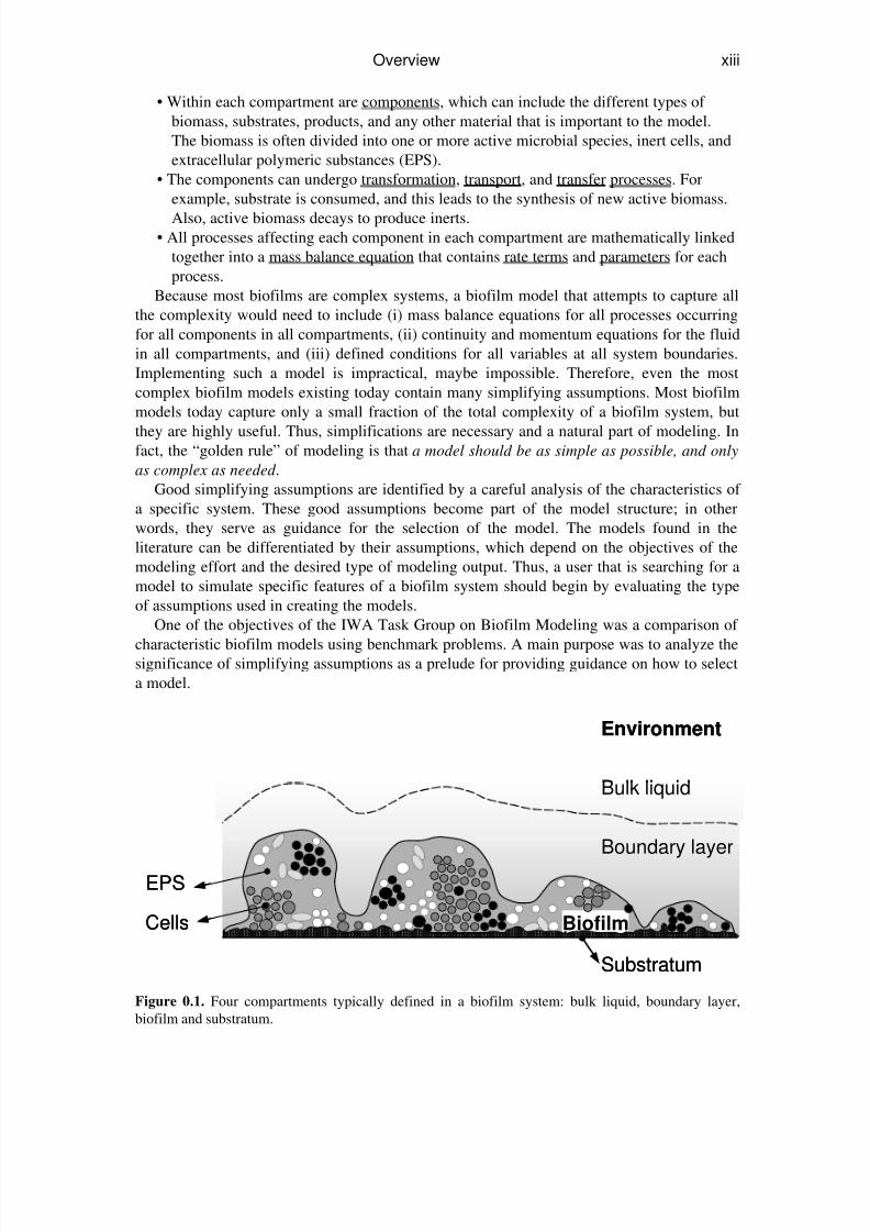
The first step in creating or choosing a biofilm model is to identify the essential features of the

biofilm system. Features are organized into a logical hierarchy that is illustrated in Figure 0.1:

• Compartments define the different sections of the biofilm system. For example, the

biofilm itself is distinguished from the overlying water and the substratum to which it is

attached. A mass-transport boundary layer often separates the biofilm from the

overlying water.



Overview xiii

• Within each compartment are components, which can include the different types of

biomass, substrates, products, and any other material that is important to the model.

The biomass is often divided into one or more active microbial species, inert cells, and

extracellular polymeric substances (EPS).

• The components can undergo transformation, transport, and transfer processes. For

example, substrate is consumed, and this leads to the synthesis of new active biomass.

Also, active biomass decays to produce inerts.• All processes affecting each component in each compartment are mathematically linked

together into a mass balance equation that contains rate terms and parameters for each

process.

Because most biofilms are complex systems, a biofilm model that attempts to capture all

the complexity would need to include (i) mass balance equations for all processes occurring

for all components in all compartments, (ii) continuity and momentum equations for the fluid

in all compartments, and (iii) defined conditions for all variables at all system boundaries.

Implementing such a model is impractical, maybe impossible. Therefore, even the most

complex biofilm models existing today contain many simplifying assumptions. Most biofilm

models today capture only a small fraction of the total complexity of a biofilm system, but

they are highly useful. Thus, simplifications are necessary and a natural part of modeling. Infact, the “golden rule” of modeling is that a model should be as simple as possible, and only

as complex as needed .

Good simplifying assumptions are identified by a careful analysis of the characteristics of

a specific system. These good assumptions become part of the model structure; in other

words, they serve as guidance for the selection of the model. The models found in the

literature can be differentiated by their assumptions, which depend on the objectives of the

modeling effort and the desired type of modeling output. Thus, a user that is searching for a

model to simulate specific features of a biofilm system should begin by evaluating the type

of assumptions used in creating the models.

One of the objectives of the IWA Task Group on Biofilm Modeling was a comparison of

characteristic biofilm models using benchmark problems. A main purpose was to analyze thesignificance of simplifying assumptions as a prelude for providing guidance on how to select

a model.

BiofilmCells

Environment

EPS

Boundary layer

Bulk liquid

Substratum

BiofilmCells

Environment

EPS

Boundary layer

Bulk liquid

Substratum

Figure 0.1. Four compartments typically defined in a biofilm system: bulk liquid, boundary layer,

biofilm and substratum.



xiv Mathematical modeling of biofilms

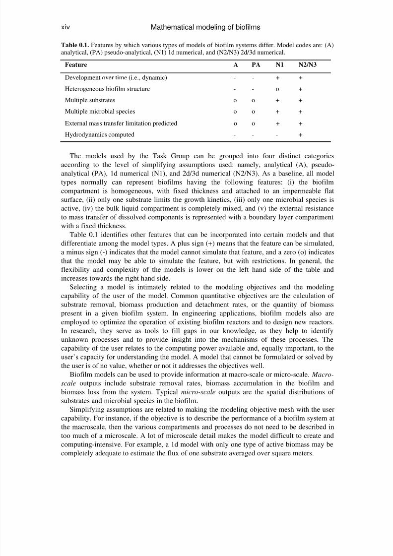
Table 0.1. Features by which various types of models of biofilm systems differ. Model codes are: (A)analytical, (PA) pseudo-analytical, (N1) 1d numerical, and (N2/N3) 2d/3d numerical.

Feature A PA N1 N2/N3

Development over time (i.e., dynamic) - - + +

Heterogeneous biofilm structure - - o +

Multiple substrates o o + +

Multiple microbial species o o + +

External mass transfer limitation predicted o o + +

Hydrodynamics computed - - - +

The models used by the Task Group can be grouped into four distinct categories

according to the level of simplifying assumptions used: namely, analytical (A), pseudo-

analytical (PA), 1d numerical (N1), and 2d/3d numerical (N2/N3). As a baseline, all model

types normally can represent biofilms having the following features: (i) the biofilm

compartment is homogeneous, with fixed thickness and attached to an impermeable flat

surface, (ii) only one substrate limits the growth kinetics, (iii) only one microbial species is

active, (iv) the bulk liquid compartment is completely mixed, and (v) the external resistance

to mass transfer of dissolved components is represented with a boundary layer compartment

with a fixed thickness.

Table 0.1 identifies other features that can be incorporated into certain models and that

differentiate among the model types. A plus sign (+) means that the feature can be simulated,

a minus sign (-) indicates that the model cannot simulate that feature, and a zero (o) indicates

that the model may be able to simulate the feature, but with restrictions. In general, the

flexibility and complexity of the models is lower on the left hand side of the table and

increases towards the right hand side.

Selecting a model is intimately related to the modeling objectives and the modeling

capability of the user of the model. Common quantitative objectives are the calculation of

substrate removal, biomass production and detachment rates, or the quantity of biomass

present in a given biofilm system. In engineering applications, biofilm models also are

employed to optimize the operation of existing biofilm reactors and to design new reactors.

In research, they serve as tools to fill gaps in our knowledge, as they help to identify

unknown processes and to provide insight into the mechanisms of these processes. The

capability of the user relates to the computing power available and, equally important, to the

user’s capacity for understanding the model. A model that cannot be formulated or solved by

the user is of no value, whether or not it addresses the objectives well.

Biofilm models can be used to provide information at macro-scale or micro-scale. Macro-

scale outputs include substrate removal rates, biomass accumulation in the biofilm and

biomass loss from the system. Typical micro-scale outputs are the spatial distributions of

substrates and microbial species in the biofilm.

Simplifying assumptions are related to making the modeling objective mesh with the user

capability. For instance, if the objective is to describe the performance of a biofilm system at

the macroscale, then the various compartments and processes do not need to be described in

too much of a microscale. A lot of microscale detail makes the model difficult to create and

computing-intensive. For example, a 1d model with only one type of active biomass may be

completely adequate to estimate the flux of one substrate averaged over square meters.



Overview xv

If the objective is to model micro-scale processes (e.g., the interaction between microbial

cells and EPS in the biofilm or 3d physical structures at the µm-scale), the number and type

of processes occurring in each compartment of the biofilm need to be represented in

microscale detail. For example, a 2d or 3d model is necessary if understanding the physical

structure of the biofilm at the µm-scale is the modeling objective, while a multi-species

model is necessary if the objective is to understand how ecological diversity develops. When

microscale detail is required, the size of the system being modeled will need to be small inorder to make the model’s solution possible.

Although many processes always take place in a biofilm, it is not necessary to include

every one, depending on the objectives. For example, the spatial distribution of the

particulate components can be specified by an a priori assumption, instead of predicted by

the model, if the goal is to predict substrate flux for a known biofilm. Then, the model needs

not include the processes of microbial growth and loss. On the other hand, when the

objective is to predict the distribution of microbial species within the biofilm or to calculate

the expected biofilm thickness at steady state, then microbial growth and detachment

processes are essential.

BIOFILM MODELSThe most basic principle for all quantitative models is conservation of mass. Conservation of

mass of a component in a dynamic and open system states that:

Net rate of Mass flow Mass flow Rate of of the of the

of mass component component of theof component component byin the system the system the system transform

= − +

accumulation production

into out of

Rate of

of thecomponent by

ations transformations

−

consumption

The local mass balances are the mathematical form of equality, which in a Cartesian

space (i.e., with ortho-normal unit vectors) can be written as

y x z j j jC r t x y z

∂∂ ∂∂ = − − − +∂ ∂ ∂ ∂

where t is time (T); x, y and z are spatial coordinates (L); C is the concentration (ML-3

); j x, j y

and j z, are the components of the mass flux j (ML-2

T-1

) along the coordinates; and r is the net

production rate (ML-3

T-1

) of the component. This is the equation of continuity for a

component, either soluble or particulate.

At the macroscopic level, global mass balances can be written based on the continuity

over the whole biofilm system. The global mass balances result also from integration of the

local balances and constitute the main engineering form of mass balance. The global mass

balances state that, for any dissolved or particulate component, the change of component

mass in time in the system is equal to the difference between component mass flow rate in

influent and effluent, plus the net production rate in the system volume. In mathematicalterms, for any component, this is written as

in ef gen

dmF F F

dt = − +

where m is the component mass (M), F in and F ef are the component mass flow rates in the

influent and the effluent (MT-1

), respectively, and F gen is the sum of the rates of all the

processes by which the component is produced or consumed (MT-1

). If two compartments, a

completely mixed “bulk liquid” and “biofilm”, are distinguished in the system, the equation

of continuity for the bulk liquid compartment becomes



xvi Mathematical modeling of biofilms

( ) B B

in ef F B

d V C F F F F

dt = − + +

where F B and F F are the overall transformation flow rates in the bulk liquid and biofilm

(MT-1

), respectively, C B is bulk liquid (and effluent, too) component concentration (ML-3

),

and finally, V B is volume of bulk liquid phase (L3).

All models analyzed in this report derive from the same general principle of mass

conservation for soluble and particulate components. The models differ, however, by the

number and the level of simplifying assumptions made to provide a solution. The most

general biofilm description would describe the development in time of a 3d distribution of

multiple soluble and multiple particulate components under diverse hydrodynamic

conditions. Due to the complexity of the mathematical description, such a model requires a

numerical solution – in fact a very sophisticated numerical solution that demands a very

high-capacity computer. However, such complex and comprehensive model is not always

necessary. The benchmark problems are good examples of settings for which much simpler

models can work well.

An analytical (A) model is the simplest solution of the general biofilm reactor model. The

determinative feature of an A model is that its solution is obtained by mathematical

derivation and without any numerical techniques. Advantages of an A solution, in addition to

its being in a simple equation format, is that the effects of each term, variable, or parameter

(e.g., diffusion coefficient, microbial kinetics, and substrate concentration) can be directly

analyzed. The disadvantage of an A solution is that the biofilm system must be very simple

to yield a mathematically derivable solution. Multiple components, complex geometries, and

time dynamics are difficult, if not impossible, to include and still have an A solution.

Analytical models are most useful for evaluating biofilm systems that have one dominant

process (e.g., nitrification or BOD removal). An A model also can be applied for multi-

species + multi-substrate systems when significant a priori knowledge of biofilm

composition is available. Analytical models are not well suited for predicting the exact

distributions of different types of bacteria in the biofilm, the conversion of multiple

substrates, the total biofilm accumulation, or complex biofilm structure.A pseudo-analytical (PA) model is a simple alternative when one or more of the

simplifications used in an A model must be eliminated to gain a realistic representation of the

biofilm system. PA solutions are comprised of a small set of algebraic equations that can by

solved directly by hand or with a spreadsheet. The solution outputs the substrate flux (J)

when the bulk-liquid substrate concentration (S) is input to it. The relative ease of using the

PA solutions makes them amenable for routine application in process design and as a

teaching tool. The pseudo-analytical solution is simply coupled with a reactor mass balance

so that the unique combination of substrate concentration and substrate flux in the reactor is

computed for a given biofilm system.

The PA solution for a steady-state biofilm was developed for single-substrate and single-

species setting, but can be applied for multi-species biofilms. Such PA solutions make multi-species modeling more accessible to students, engineers, and non-specialist researchers. In

addition, creating and using a multi-species PA model illuminates the important interactions

that take place among the different types of biomass in a multi-species biofilm.

The numerical 1d (N1) models represent multi-species and multi-substrate biofilms in one

dimension perpendicular to the substratum. Their complexity lies between the simpler A and

PA models and the numerically demanding multi-d models. The N1 model equations must be

solved numerically, but even complex simulations can be performed on a PC within minutes.

The most significant feature of an N1 model is its flexibility with regard to the number of

dissolved and particulate components, the microbial kinetics, and to a certain extent also the



Overview xvii

physical and geometrical properties of the biofilm. An N1 model can be used as a tool in

research, as well as for the design and simulation of biofilm reactor. Already available

commercial simulation software that implements such N1 models make also dynamic multi-

species modeling accessible to students, engineers, and non-specialist researchers.

Examples of particulate components are active microbial species, organic and inorganic

particles, and EPS. Examples of dissolved components are organic and inorganic substrates,

metabolites, products, and the hydrogen ion. The output produced by the N1 model includes• Spatial profiles of any number of particulate components in the biofilm

• Accumulation and the loss from the system of the mass of the particulate

components

• Spatial profiles of any number of dissolved components in the biofilm

• Removal rates and effluent concentrations of the dissolved components

• Biofilm thickness as a function of the production and decay of particulate material in

the biofilm and of attachment and detachment of cells and particles at the biofilm

surface and in the biofilm interior

For all these quantities, the development in time, as well as steady state solutions, can be

calculated.

Numerical 2d and 3d (N2 and N3) models are used to describe the heterogeneouscharacteristics of biofilms. The premise is that, by capturing the spatial and temporal

heterogeneity of the physical, chemical, and biological environment, the model makes it

possible to assess biofilm activity and interactions at the microscale. New problems to be

addressed by multi-dimensional biofilm models include, for example:

• Geometrical structure of biofilms: How does the spatial biofilm structure form? What

is the influence of environmental conditions on the biofilm structure? How does

quorum sensing operate? What causes biomass detachment? How does microbial

motility influence biofilm formation?

• Mass transfer and hydrodynamics in biofilms: What is the importance of advective

mass transport relative to diffusion in the biofilm? How does the biofilm’s spatial

structure affect the overall solute transport rates to/from the biofilm?• Microbial distribution in biofilms: What is the importance of inter-species substrate

transfer? What is the influence of substrate gradients on microbial competition and

selection processes?

The main difference between N1 and N2/N3 models is in the way processes affecting the

development of the solid biofilm matrix and the dynamics of its composition (i.e., biomass

growth, decay, detachment and attachment) are represented. For example, when second or

third dimensions are part of the physical domain being modeled, the biofilm matrix has more

than one direction in which to grow, allowing the simulation of spatially heterogeneous

biofilms. Other potentially important phenomena that can be included with a multi-d model

are fluid motion and advective mass transport in and out of the biofilm. Another class of

addressed problems concerns the interaction among biofilm shape, fluid flow, biomassdecay, and biofilm detachment.

Of course, allowing more complexity in the model increases the computing requirements

dramatically. However, although initially some of the N2 and N3 models were coded and run

using high performance supercomputers, nowadays, most multi-d biofilm models can be

executed on single-processor machines.



xviii Mathematical modeling of biofilms

BENCHMARK PROBLEMS

The benchmark problems help identify the trade offs inherent to using the different types of

models. Because each model solves the same benchmark problem, the differences of the

output produced by the models reflect the differences of the model complexity and of the

simplifying assumptions that are made in the various models.

The first benchmark problem (BM1) describes nearly the simplest system possible: amono-species biofilm that is flat and microbiologically homogeneous. Benchmark problem 2

(BM2) evaluates the influence of hydrodynamics on substrate mass transfer and conversions

in a geometrically heterogeneous biofilm. Benchmark problem 3 (BM3) describes

competition between different types of biomass in a multi-species and multi-substrate

biofilm. Because the benchmark problems were designed to evaluate the ability of the

models to represent fundamental features of a biofilm system, the trends apply to biofilms in

treatment technology, nature, and situations in which biofilm is unwanted.

• BM1 describes a simple flat, mono-species biofilm. BM1 gives a baseline comparison

of the different biofilm models for a biofilm system that is well suited for any modeling

approach. The specific objective of BM1 is to compare key outputs, particularly including

effluent substrate concentrations and substrate flux. Furthermore, the user friendliness of the

different modeling approaches is evaluated.

For the simple conditions of BM1, modeling results are not significantly different for all

modeling approaches having flat biofilm morphology. On the other hand, modeling results

are strongly influenced by the assumption for mass transfer in the pores within the biofilm

when heterogeneous biofilm morphology is allowed.

While modeling results are similar for most modeling approaches, the effort in

implementing and using the different models is not. A and PA models can be readily solved

using a spreadsheet. However, A or PA solutions require a number of simplifications, and the

modeler has to make a priori decisions, e.g., on the dissolved component that is rate limiting.

N1 models can be solved readily on a PC using available software. N2 and N3 models are

able to simulate heterogeneous biofilm morphology, but they require custom-made software

and, in some situations, extensive computing power. To approximately evaluate the influence

of a heterogeneous morphology, N1 simulations can be combined to create pseudo-N3

models.

Thus, for simple biofilm systems and more-or-less smooth biofilm surfaces, A, PA, or N1

models often provide good compromise between the required accuracy of modeling results

and the effort involved in producing these results. Adopting the more complex and intensive

N2 and N3 models is justified only when the heterogeneity that they allow is critical to the

modeling objective.

• BM2 involves spatially heterogeneous architectures that can induce complex flow

patterns and affect mass transport. Classical 1d biofilm models are not able to capture this

kind of complexity, which historically has been one of the reasons for the development of

multi-d models.Specifically, the assumption of a completely mixed bulk fluid is given up in this

benchmark problem, and mass transport due to diffusion and advection in the fluid

compartment are explicitly considered. The latter implies that the hydrodynamic flow field

should be taken into account as well. A direct micro-scale mathematical description leads to

a non-linear system of 3d partial differential equations in a complicated domain, and this is

numerically expensive and difficult to solve. Therefore, BM2 investigates to what extent

such a detailed local description of physical and spatial effects is necessary for macro-scale

applications, where the purpose of the modeling is often only to calculate the total mass



Overview xix

fluxes into the biofilm, i.e., the global mass conversion rates. To this end, the description of

the physical complexity of the system, expressed in geometrical and hydrodynamic

complexity, can be simplified in various ways and to varying degrees in order to obtain faster

simulation methods. The results of these simplified models are compared with the results for

the fully 3d simulations.

Due to the high computational demand of 3d fluid dynamics in irregular domains, the

problem is restricted to a small section of a biofilm (1.6 mm long). The goal of BM2 is tocalculate: (1) the flux of dissolved substances into the solid region and, (2) the average

substrate concentrations at the solid/liquid interface and at the substratum. A crucial aspect of

the formulation of BM2 is the specification of appropriate boundary conditions. These are

required to connect the small computational system with the external world that surrounds

the modelling domain.

The 1d, 2d, and 3d models considered showed the same general sensitivities towards

changes in biofilm thickness and hydrodynamics and were able to describe the qualitative

system behavior. For the quantitative details, the key to a successful model reduction is a

good description of the hydrodynamic conditions in the reactor segment. In a 2d reduction,

this can be accomplished by a 2d version of the governing flow equations. The 1d

approaches require a global mass balance or an empirical correlation that incorporates thehydrodynamics with passable reliability and accuracy.

Which simplified predictive model offers the best effort/accuracy/reliability trade-off

depends largely on the hydrodynamic regime. Therefore, an analysis of the flow conditions

in the reactor is required first before a simplification should be applied. Due to the enormous

requirement of input data, the application of 3d models including full hydrodynamic

calculations is restricted. These statements are made for applications in which only global

results are of interest; that is, no refined resolution of the processes inside the biofilm is

required. If such local results are desired, 1d models cannot yield a good description for

spatially heterogeneous biofilms. At least a 2d model must be applied and, hence, the

required input data and computing power must be provided.

• The goal of multi-species BM3 is to evaluate the ability of the different biofilm modelsto describe microbiological competition. In particular, BM3 focuses on competition for the

same substrate and the same space in a biofilm. Together, these competitions provide a

rigorous test for modeling multi-species biofilms, but without introducing unnecessary

complexity.

To meet the goal, BM3 includes three biomass types having distinctly different metabolic

functions:

- aerobic heterotrophs

- aerobic, autotrophic nitrifiers

- inert (or inactive) biomass

This scenario represents a common situation for biofilms in nature and in treatment processes

for wastewater and drinking water.For simplicity and comparability, BM3 uses the same physical domain as BM1: a flat

biofilm substratum in contact with a completely mixed reactor experiencing a steady flow

rate. To avoid unnecessary complexity, BM3 treats the nitrifiers as one "species" that

oxidizes NH4+-N directly to NO3

--N. Thus, it does not consider the intermediate NO2

-or the

division of nitrifiers between ammonia oxidizers and nitrite oxidizers. Active heterotrophs

and nitrifiers follow Monod kinetics for substrate utilization and synthesis. They also

undergo decay following two paths: (1) lysis and oxidation by endogenous respiration, and

(2) inactivation to form inert or inactive biomass. The inert biomass does not consume



xx Mathematical modeling of biofilms

substrate, and it is not consumed by any reactions. All forms of biomass can be lost by

physical detachment.

The results of BM3 demonstrate that a wide range of 1d models is capable of representing

the important interactions that can occur in biofilms in which distinctly different types of

biomass can co-exist. The choice of the model depends on the user's needs and the modeling

situation. One key choice is between models that demand a full numerical solution versus

those that can be implemented with a spreadsheet. A second choice concerns the way inwhich the biomass is distributed. By far the simplest approach is to assume that the biomass

types are independent of each other. This approach may work well when protection of a

slow-growing species (like the nitrifiers) or dilution of a fast-growing species (like the

heterotrophs) is not a major issue. When protection of a slow-growing species is critical to an

accurate representation, then a model that accumulates the slow growers away from the outer

surface is essential. When the dilution of a fast-growing species by slower growers is key,

then a model that distributes the different biomass types throughout the biofilm is essential.

BM3 also was solved with two N2 models, which produce results similar to two N1

models for bulk substrate concentrations and fluxes into the biofilm. The similarity in output

parameters for substrate concentration and fluxes is likely the result of the system in BM3

being a flat biofilm in a completely mixed reactor. On the other hand, the predicteddistributions of the different types of biomass varied considerably between N1 and N2

models. In this regard, the only identifiable trend when comparing the N1 to the N2 models

is the apparent increased, stable protection of nitrifiers in the N1 models, especially when

this population is affected by a large accumulation of inerts or a lower rate of oxygen

utilization. This trend likely reflects the different mechanisms to distribute the biomass

within the biofilm.

Mathematical Modeling of Biofilms Abstract Isbn1843390876 Contents

Documents

Transcript of Mathematical Modeling of Biofilms Abstract Isbn1843390876 Contents