Mathematical Modeling for Optimal Design of

In-Building Distributed Antenna Systems

Lei Chen and Di Yuan

Linköping University Post Print

N.B.: When citing this work, cite the original article.

Original Publication:

Lei Chen and Di Yuan, Mathematical Modeling for Optimal Design of In-Building

Distributed Antenna Systems, 2013, Computer Networks, (57), 17, 3428-3445.

http://dx.doi.org/10.1016/j.comnet.2013.07.027

Copyright: Elsevier

http://www.elsevier.com/

Postprint available at: Linköping University Electronic Press

http://urn.kb.se/resolve?urn=urn:nbn:se:liu:diva-89716

Mathematical modeling for optimal design of in-building

distributed antenna systems

Lei Chen∗, Di Yuan

Department of Science and Technology, Linkoping University, Sweden

Abstract

In-building Distributed Antenna System (IB-DAS) has proven to be one ofthe most promising In-Building Solutions (IBS) to provide coverage and ca-pacity for indoor users. We consider optimal deployment of the passiveIB-DAS, focusing on mathematical optimization models based on integerprogramming, for the topology design and optimal equipment selection ofIB-DAS. The models minimize the cable cost and keep the transmit powerat each antenna within a given interval defined for coverage and interferencecontrol. The models can deliver optimal solutions to systems of which thesize is of practical relevance. To improve the time efficiency, we develop pre-processing techniques that integrate the building layout data into the systemmodeling. Application of the models to realistic IB-DAS deployment demon-strates the effectiveness of the models.

Keywords: distributed antenna systems, integer programming,optimization

1. Introduction

Providing sufficient coverage and capacity for indoor users has alwaysbeen a challenge for the mobile operators. With the evolution of cellulartechnologies, in-building traffic has grown dramatically. Today, over 80% ofmobile data traffic and 70% of voice traffic are generated by in-building users[1]. The fast development and deployment of the next generation cellularnetworks, such as Long Term Evolution (LTE) will push the in-building trafficto an even higher level, making it the main revenue generator for the mobile

∗Corresponding author

Preprint submitted to Computer Networks January 10, 2014

operators. Thus, it has become crucial for the operators to deploy dedicatedin-building systems to fulfill the increasing indoor data requirements.

The demand of in-building users is a performance bottleneck for the over-all performance of cellular networks, and insufficient in-building coveragecontributes largely to the degradation of the overall network throughput ofthe macro-cells [2, 3]. For in-building users, the main reason for the poorsignal level is due to the loss of signal strength for wall penetration. The lossvalue is within the range of 20 and 50 dB [9]. With the migration from lowerfrequency bands of GSM (e.g., 800 MHz and 900 MHz) to higher frequencybands of LTE (e.g., 2.4 GHz), the signal loss from wall penetration becomeshigher. For a concrete wall that results in 20 dB penetration loss for GSM at800/900 MHz, the corresponding loss for LTE is more than 30 dB and hencesignificantly higher. The existence of metals in the wall, such as lead, intro-duces further attenuation. In addition to wall penetration, the orthogonalityof the radio channels can be compromised because of multi-path reflectionsfor the in-building coverage of Universal Mobile Telecommunications System(UMTS) networks. In-building Distributed Antenna System (IB-DAS) hasproven to be one of the most promising methods for dedicated in-buildingsolutions. With a properly deployed IB-DAS system, a favorable link budget,i.e., better radio signal reception, can be provided because of the absence ofwall penetration requirement and less impact of multi-path reflections. Also,coverage holes can be easily avoided by a careful planning of the distributedantennas, as well as the use of directional antennas. As a result, in-buildingusers will experience a satisfactory level of network presence. Besides, IB-DAS can help offload the macro-cell network traffic significantly. In addition,the average downlink transmission power of the base station can be reduced,making more system capacity available to macro-cells for serving outdoorusers. Uplink transmission power can also be reduced significantly so that amuch longer battery life can be achieved for the user equipments.

A major type of IB-DAS is Passive DAS (P-DAS). In this paper, weconsider optimal deployment of P-DAS. A typical P-DAS consists of a centerbase station (BS) and a number of distributed antennas. The BS uses adonor antenna on the roof of the building to connect to the macro-cell forregular communication service as well as to specialized public safety site foremergency service. Distributed antennas are connected to the center BS viacopper coaxial cable. Power equipments, such as splitters and taps, are usedto split and distribute the power towards the antennas. P-DAS has beenextensively used for cost-effective indoor access in small buildings.

2

Previous works of DAS planning mostly concentrate on the performancegains brought by the deployment of DAS for the in-building scenarios. In [4],the authors study the performance gain of DAS both by analytical reasoningand system simulations. The work in [5] compares the results of the DASsystem with a conventional Array Antenna System (AAS). The author of [6]discusses the importance of a dedicated in-building solution for 3G networks.In [7], the authors propose to use repeaters based on DAS deployment forcapacity improvement of UMTS networks. All these works have pointed outthe importance of a proper deployment of IB-DAS in order to bring significantperformance gains to in-building users. An optimization-oriented study of P-DAS deployment is provided in [8]. The DAS Forum [9] has dedicated itselfto the promotion and development of the DAS solutions, and provides casestudies of DAS in various fields, e.g., regular data services, health care, publicsafety, and so on.

From the planning point of view, deployment of IB-DAS systems amountsto constructing an optimal topology which connects all distributed antennasto the center BS, and selecting equipments at the intermediate nodes. Toguarantee the performance, the output power of each antenna, which is de-termined by both the topology and equipment selection, is confined to bea pre-defined interval. Cable usage, which contributes to the most of theoverall cost of the deployment of IB-DAS, is minimized. We approach theproblem from a mathematical programming standpoint, and develop mixedinteger programming models for problem solution. Preprocessing techniquesutilizing the building structure have been introduced to strengthen the com-putational efficiency of the models. We present numerical results demon-strating that our solution approach enables the optimal deployment solutionof IB-DAS systems of realistic size.

The rest of the paper is organized as follows. Section 2 gives a detailedpresentation of the P-DAS. Section 3 introduces notation, and performs sys-tem modeling of DAS deployment. Two mixed integer linear programmingmodels are presented and detailed in Sections 4 and 5, respectively. Pre-processing techniques for enhancing the computational efficiency are devel-oped in Section 6. Section 7 presents performance evaluation of the solutionapproach for realistic IB-DAS deployment scenarios. Section 8 concludes thepaper and discusses future works.

3

2. Distributed antenna system

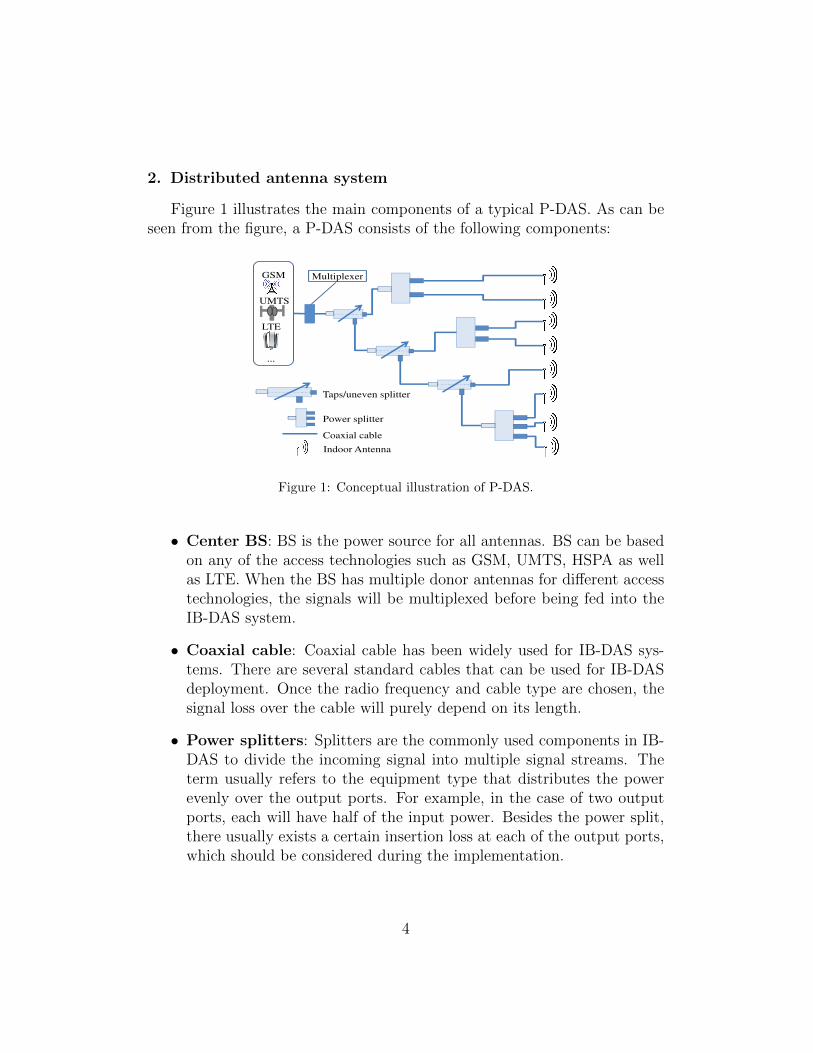
Figure 1 illustrates the main components of a typical P-DAS. As can beseen from the figure, a P-DAS consists of the following components:

UMTS

GSM

Power splitter

Coaxial cable

Indoor Antenna

Taps/uneven splitter

LTE

���

Multiplexer

Figure 1: Conceptual illustration of P-DAS.

• Center BS: BS is the power source for all antennas. BS can be basedon any of the access technologies such as GSM, UMTS, HSPA as wellas LTE. When the BS has multiple donor antennas for different accesstechnologies, the signals will be multiplexed before being fed into theIB-DAS system.

• Coaxial cable: Coaxial cable has been widely used for IB-DAS sys-tems. There are several standard cables that can be used for IB-DASdeployment. Once the radio frequency and cable type are chosen, thesignal loss over the cable will purely depend on its length.

• Power splitters: Splitters are the commonly used components in IB-DAS to divide the incoming signal into multiple signal streams. Theterm usually refers to the equipment type that distributes the powerevenly over the output ports. For example, in the case of two outputports, each will have half of the input power. Besides the power split,there usually exists a certain insertion loss at each of the output ports,which should be considered during the implementation.

4

• Power taps: If all antennas have similar range of coverage, it is de-sirable that they have roughly the same output power [10]. The usageof power splitters may not be enough to achieve this because in manycases some distributed antennas are very near to the BS whereas oth-ers are far away. Taps, also referred to as uneven splitters, are usedto tap a small portion of the power along the cable and leave the restfor serving antennas located further away. The installation of powersplitters and taps is a key issue in IB-DAS planning as it plays therole of distributing the power for the purpose of coverage and capacityguarantee.

• Distributed antennas: Distributed antennas are the terminals of theIB-DAS. They serve as the access points for the in-building users. Thelocation and desired output power of the antennas are typically deter-mined from a radio access planning tool that, based on expected userdistribution and traffic demand, selects the locations and the powerlevels such that sufficient coverage is provided and the interference be-tween the antennas is acceptable. The output power levels are thuspart of the input to topology design and equipment selection. In mostof the cases, it is not necessary or even possible to meet the target levelexactly. Usually, a threshold can be used to limit the power deviationof each antenna.

3. System modeling

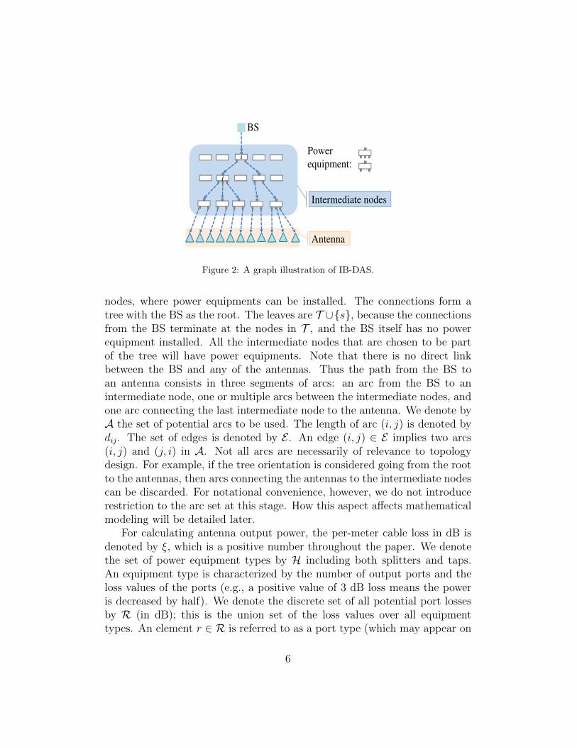
IB-DAS design is an optimization problem over a graph. There are twosets of nodes in addition to the BS node. The first set consists of the dis-tributed antennas. The second set is composed by candidate locations, re-ferred to as intermediate nodes henceforth, for power equipment installation.The locations of the intermediate nodes are pre-chosen by considering thebuilding structure as well as the easiness for equipment installation. Thetopology of an IB-DAS is a rooted tree originating from the BS and connectsall distributed antennas through cables and power equipments, see Figure 2for an illustration.

To represent the graph, we introduce the following notation. We denotethe BS by s and the set of intermediate nodes by N . The set of antennas isdenoted by T . For each antenna t ∈ T , ptart denotes the target output power.All distributed antennas will connect to the BS through the intermediate

5

BS

�

�

Power

equipment:

Intermediate nodes

Antenna

Figure 2: A graph illustration of IB-DAS.

nodes, where power equipments can be installed. The connections form atree with the BS as the root. The leaves are T ∪{s}, because the connectionsfrom the BS terminate at the nodes in T , and the BS itself has no powerequipment installed. All the intermediate nodes that are chosen to be partof the tree will have power equipments. Note that there is no direct linkbetween the BS and any of the antennas. Thus the path from the BS toan antenna consists in three segments of arcs: an arc from the BS to anintermediate node, one or multiple arcs between the intermediate nodes, andone arc connecting the last intermediate node to the antenna. We denote byA the set of potential arcs to be used. The length of arc (i, j) is denoted bydij. The set of edges is denoted by E . An edge (i, j) ∈ E implies two arcs(i, j) and (j, i) in A. Not all arcs are necessarily of relevance to topologydesign. For example, if the tree orientation is considered going from the rootto the antennas, then arcs connecting the antennas to the intermediate nodescan be discarded. For notational convenience, however, we do not introducerestriction to the arc set at this stage. How this aspect affects mathematicalmodeling will be detailed later.

For calculating antenna output power, the per-meter cable loss in dB isdenoted by ξ, which is a positive number throughout the paper. We denotethe set of power equipment types by H including both splitters and taps.An equipment type is characterized by the number of output ports and theloss values of the ports (e.g., a positive value of 3 dB loss means the poweris decreased by half). We denote the discrete set of all potential port lossesby R (in dB); this is the union set of the loss values over all equipmenttypes. An element r ∈ R is referred to as a port type (which may appear on

6

multiple equipment types) with r dB loss. To denote the relation betweenport loss r ∈ R and each of the power equipment types h ∈ H, we introducea parameter αrh, r ∈ R, h ∈ H which specifies how many ports (possiblyzero) with loss r ∈ R are present for equipment type h.

In the deployment of IB-DAS, coaxial cable cost usually dominates the to-tal expenditure. Thus the optimal deployment should use a minimum amountof cable. In addition, from the DAS performance viewpoint, the deploymentis driven by the power targets of the antennas. Having output powers closeto the targets ensures the coverage and capacity for the in-building users foreach antenna, and keeps the signal leakage to outdoor users at a minimumlevel. In many cases, it is not possible to meet exactly the power targetsusing the cable connections and power equipment types at choice. One wayof system modeling is to minimize the deviation from the power targets, andweight this quantity in the objective function. However, finding a properweight is far from trivial. Furthermore, a potential problem is the result ofa very uneven power distribution among the in-building antennas, leadingto significant coverage holes and signal leakage. In this paper, we apply athreshold, denoted by pthrt (t ∈ T ), to bound the absolute difference betweenthe power target and the achieved value. If the threshold is too stringent,the topology design and equipment type selection problem may be infeasible.To deal with such a case, the problem can be solved with several thresholdvalues to generate multiple candidate design solutions.

Optimal deployment of IB-DAS amounts to designing a tree having theBS s as the root and the antennas as the leaves, and the selection of anequipment type for each intermediate tree node as well as a port assignmentfor the outgoing arcs of the node. The objective of the deployment is tominimize the total cable cost, with constraints representing the power devi-ation threshold. There is no doubt that the problem is NP-hard. Indeed,the well-known and NP-hard Steiner arborescence problem [11] reduces tothe IB-DAS deployment problem. A sketch of the reduction consists in thefollowing. First, for each terminal node of the Steiner arborescence problem,there is one antenna to which the terminal node provides the only possibledirect connection. Second, an extra node is introduced for the source (whichis restricted to have degree one in IB-DAS). The extra node, to be connectedwith intermediate nodes, is the only possible connection from the source.Third, the power threshold is large enough to be redundant and there is norestriction on the number of ports, i.e., there is one equipment type availablefor each possible out-degree. After the reduction, the two problems become

7

equivalent, and the NP-hardness of IB-DAS deployment follows. For ourpractical application with IB-DAS planning scenarios where the size is natu-rally set by the deployment process (e.g., the design of one floor is typicallyde-coupled from that of other floors), striving for optimality with a reason-able amount of computational effort is not only desirable, but also potentiallyfeasible by means of integer programming.

From the discussion thus far, it is clear that optimal IB-DAS deploymentis a type of network design problem, for which mathematical modeling andinteger linear programming have been successfully used in various applica-tions [12, 13, 14, 15, 16, 17]. On the other hand, the IB-DAS optimizationproblem has its peculiarities, in particular the tasks of equipment selectionand port assignment, that are not present in classical network design appli-cations. In this paper, our goal is to apply advanced integer programmingmodeling to enable to approach optimal or near-optimal solutions for IB-DASdeployment for planning scenarios of practical size. We develop two mod-eling approaches relying on very different concepts. The first uses networkflows to enforce connection from the source to the antennas, and the secondis based on the idea that undirected Steiner tree can be viewed as a numberof Steiner arborescences.

4. Flow formulation (DAS-F)

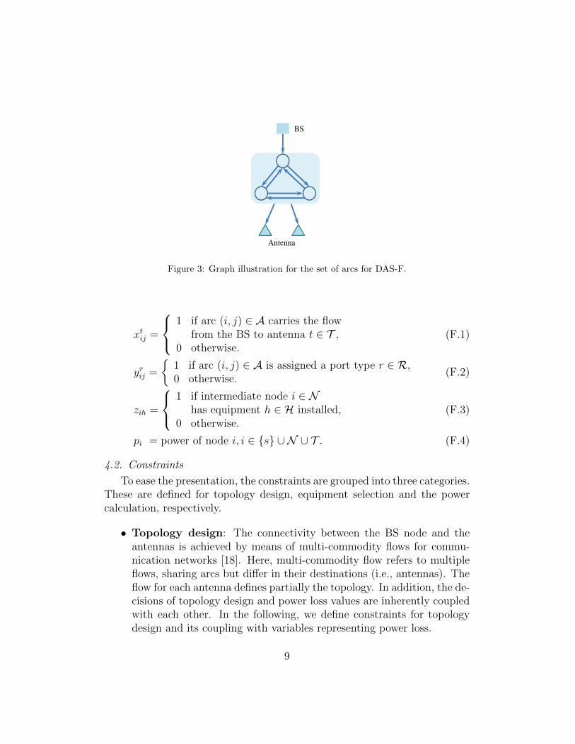
The notion of source-destination flow is commonly used for formulatingnetwork design problems. In this section, we develop a flow formulation,denoted by DAS-F, for IB-DAS deployment. In DAS-F, the arc setA containsarcs from the BS to the intermediate nodes, arcs between the intermediatenodes, and finally the arcs from the intermediate nodes to the antennas, seeFigure 3 for an illustration. Arcs from the antennas to the intermediatenodes as well as arcs from the intermediate nodes to the BS are discardedin the model, because the flow goes only in the direction from the BS to theantennas.

4.1. Decision variables

In DAS-F, the tree topology is enforced by introducing a unit of flow fromthe BS to each antenna. Additional design decisions include the selection ofequipment (splitters or taps) with a specific type for each intermediate treenode, and the mapping between the ports and the outbound arcs. To theseeffects, we introduce the following four sets of variables.

8

BS

Antenna

Figure 3: Graph illustration for the set of arcs for DAS-F.

xtij =

1 if arc (i, j) ∈ A carries the flow

from the BS to antenna t ∈ T ,0 otherwise.

(F.1)

yrij =

{1 if arc (i, j) ∈ A is assigned a port type r ∈ R,0 otherwise.

(F.2)

zih =

1 if intermediate node i ∈ N

has equipment h ∈ H installed,0 otherwise.

(F.3)

pi = power of node i, i ∈ {s} ∪ N ∪ T . (F.4)

4.2. Constraints

To ease the presentation, the constraints are grouped into three categories.These are defined for topology design, equipment selection and the powercalculation, respectively.

• Topology design: The connectivity between the BS node and theantennas is achieved by means of multi-commodity flows for commu-nication networks [18]. Here, multi-commodity flow refers to multipleflows, sharing arcs but differ in their destinations (i.e., antennas). Theflow for each antenna defines partially the topology. In addition, the de-cisions of topology design and power loss values are inherently coupledwith each other. In the following, we define constraints for topologydesign and its coupling with variables representing power loss.

9

Constraints (F.5) require that for any antenna t, there is exactly oneunit of flow sent from the source BS node. As there is no power equip-ment at the BS, all flows originating from the BS will share a commonarc. This is modeled by constraints (F.6). Each antenna is the des-tination of exactly one unit of flow, as specified by (F.7). Constrains(F.8) define flow conservation at the intermediate nodes, that is, theincoming flow and outgoing flow of each antenna must be in balance.Constraints (F.9)-(F.11) represent the coupling relation between topol-ogy and the presence of power loss. By (F.9), at least one port typewill be chosen for arc (i, j), if the flow towards antenna t goes throughthe arc. Conversely, if a port type is selected for arc (i, j), then theremust be at least one antenna t whose flow passes this arc, as stated byconstraints (F.10). Constraints (F.11) are the equality form of (F.9) forarcs having antenna as their end nodes. The equality sign stems fromthe facts that, for any antenna t, exactly one of the incoming arcs mustbe chosen, and one power loss value must be selected for the startingnode of the arc. Finally, constraints (F.12) state that for each node j,equipment power loss occurs on at most one incoming arc. As a result,the flows will be constrained on a tree topology.

∑j∈N :(s,j)∈A

xtsj = 1, ∀t ∈ T (F.5)

xt1sj = xt2sj, ∀t1, t2 ∈ T , j ∈ N :

t1 6= t2, (s, j) ∈ A (F.6)∑j∈N :(j,t)∈A

xtjt = 1, ∀t ∈ T (F.7)

∑j∈N :(j,i)∈A

xtji =∑

j∈N :(i,j)∈A

xtij, ∀t ∈ T , i ∈ N (F.8)

xtij ≤∑r∈R

yrij, ∀(i, j) ∈ A, t ∈ T , i 6= s (F.9)

yrij ≤∑t∈T

xtij, ∀(i, j) ∈ A, r ∈ R, i 6= s (F.10)

xtit =∑r∈R

yrit, ∀i ∈ N , t ∈ T : (i, t) ∈ A (F.11)

10

∑i∈N :(i,j)∈A

∑r∈R

yrij ≤ 1, ∀j ∈ N (F.12)

• Power equipment selection: Power equipment selection involvesboth equipment type and the port-to-arc assignment for each interme-diate node of the tree. The following constraints ensure that, if anyflow passes through an intermediate node, then an equipment type hasto be selected and all the ports are used.

∑h∈H

zih ≤ 1, ∀i ∈ N (F.13)∑r∈R

yrij +∑r∈R

yrji ≤ 1, ∀i, j ∈ N , (i, j) ∈ A (F.14)∑j∈N∪T :(i,j)∈A

yrij =∑h∈H

zihαrh, ∀i ∈ N , r ∈ R (F.15)

By (F.13), at most one equipment type can be present at any interme-diate node. For any two intermediate nodes i, j ∈ N , only one of thetwo arcs (i, j) and (j, i) will be used to route the flow from the source,and thus at most one of the two ends will have equipment power loss.This is defined by constraints (F.14). Next, constraints (F.15) give theeffect that all ports of an installed equipment are used for connections.Note that at most one z-variable in the right-hand side of (F.15) can beone. Thus, for each node i and possible power loss value r, the right-hand side of (F.15) is the total number of outgoing ports (possibly zero)with loss r at node i. This number must be equal to the number ofoutgoing arcs that are assigned the corresponding value. The latter isgiven by the sum in the left-hand side.

• Power constraints: The last category of constraints is used to applypower calculation in connection with the other decisions made, alongwith enforcing the power deviation threshold of the antennas. Recallthat the power loss occurs along the cables and at the equipment ports.For any of the two nodes i, j ∈ N ∪ T and the arcs between them, thepower loss can be calculated as follows.

11

pj = pi − ξdij − r, if and only if yrij = 1 (F.16)

By (F.16), the power of node j equals that of node i minus the distance-based cable loss and the loss caused by i’s equipment with connectionto j, if the corresponding y-variable is one. Because only one equipmentloss value is assigned to any arc by (F.12), the equation can be rewrittenover all possible equipment loss values as follows.

pj = pi − ξdij∑r∈R

yrij −∑r∈R

ryrij, if and only if∑r∈R

yrij = 1 (F.17)

Power calculation for arcs leaving the BS has to be performed in aslightly different way, for the reason that no equipment is installed atthe BS, for which no y-variable is present. Instead, the x-variables areused to set the condition for power calculation, and the loss originatesfrom the arc length only, as formulated below. Note that the power ofthe source node ps is also a variable.

pj = ps − ξdsj, if and only if xtsj = 1,∀t ∈ T (F.18)

In the IB-DAS tree topology, exactly one arc from the BS is selected.The selected arc carries flows towards all |T | antennas. Thus, if anyarc (s, j), j ∈ N is chosen, all flows go through that arc, meaning that∑

t∈T xtsj = |T |. Thus, the power can be calculated as follows for the

arcs from the BS.

pj = ps −∑

t∈T ξdsjxtsj

|T |, if and only if

∑t∈T

xtsj = |T | (F.19)

Equations (F.17) and (F.19) are non-linear, because of the if-and-only-if statement. To reach linearity, the equality is represented by twoinequalities, and a parameter M , referred to as big M, is used. Thelinear reformulations for power calculation are presented below.

12

pj ≤ pi − ξdij∑r∈R

yrij −∑r∈R

ryrij +M(1−∑r∈R

yrij),

∀i, j ∈ N ∪ T : (i, j) ∈ A (F.20)

pj ≥ pi − ξdij∑r∈R

yrij −∑r∈R

ryrij −M(1−∑r∈R

yrij),

∀i, j ∈ N ∪ T : (i, j) ∈ A (F.21)

pj ≤ ps −ξdsj

∑t∈T x

tsj

|T |+M(1−

∑t∈T x

tsj

|T |),

∀j ∈ N : (s, j) ∈ A (F.22)

pj ≥ pi −ξdsj

∑t∈T x

tsj

|T |−M(1−

∑t∈T x

tsj

|T |),

∀j ∈ N : (s, j) ∈ A (F.23)

In (F.20), the power of node j is bounded from above by the powercalculation in (F.18), if

∑r∈R ry

rij = 1. Otherwise the last term will

be at least M , and the inequality does not pose any constraint on thepower of j if M is sufficiently large (e.g., the sum of the cable loss ofall potential arcs). Constraints (F.21) are similar in construction, withthe effect of bounding the power of j from below if

∑r∈R ry

rij = 1.

Thus these two constraints together achieve the effect of (F.18). Thefollowing two constraints carry the same notion for replacing (F.19).The power constraints become complete by setting the threshold re-quirement at the antennas, as stated below.

pthrt ≥ ptart − pt, ∀t ∈ T (F.24)

pthrt ≥ pt − ptart , ∀t ∈ T (F.25)

.

4.3. Objective function

The objective function is to minimize the total amount of cabling. Thisis formulated below.

13

∑(s,j)∈A

∑t∈T

dsjxtsj

|T |+

∑(i,j)∈A:i 6=s

dij∑r∈R

yrij (F.26)

In (F.26), the first term is the cable length from the BS. Because all flowswill be on a single arc from the BS, the sum is divided by |T | to obtain thecable length. The second term gives the total cable length originating fromthe intermediate nodes.

4.4. Model summary

Putting the pieces together, optimal deployment of IB-DAS using net-work flows can be made by the following mixed integer linear programmingformulation.

[DAS− F] : min (F.26)

s.t. (F.6)− (F.15), (F.20)− (F.23), (F.24), (F.25).

With the notion of network flow, formulation DAS-F is fairly straightfor-ward. However, its applicability for problem solving is limited to small-scaleplanning scenarios. The main reason is the presence of the big-M parameter,making the continuous relaxation of DAS-F rather weak in approximatingthe integer optimum.

5. Multi-tree formulation (DAS-MT)

Our second modeling approach, which explores the concept of multi-tree,is less trivial than the use of network flows. Recall that the topology ofIB-DAS assembles a Steiner tree, with the difference that all antennas inID-DAS must be tree leaves. An undirected Steiner tree can be viewed asmany Steiner arborescences with different root nodes [19, 20]. Moreover,the multiple arborescences can be coupled together to share a common treetopology. Applying the concept, for IB-DAS the topology can be viewed as1+ |T | arborescences rooted at the BS and the antennas, respectively. Theseare the leaves in the common tree. Hereafter, we refer to the model basedon the concept of multi-tree as DAS-MT.

DAS-MT uses both the edge set E and the arc set A. The definition of theset of arcs is slightly different from that for DAS-F. Specifically, arcs adjacent

14

to the BS are reversed. Thus only arcs having BS and the antennas as theend nodes are included in set A in DAS-MT. The arcs between intermediatenodes remain. The composition is illustrated in Figure 4.

BS

Antenna

Figure 4: Graph illustration of the arcs in DAS-MT.

5.1. Decision variables

In DAS-F, the flow on each arc and the port type choice of each arcare denoted by xtij and yrij, respectively. In DAS-MT, the key variables, asdefined below, consider the joint effect of arc use and port type selection.

qrkij =

1 if arc (i, j) is used to reach node k with port type r,

for node k ∈ {s} ∪ T \ {j},0 otherwise.

(MT.1)

The rationale of variable qrkij is to specify the orientation of using arc(i, j) to reach node k in the tree, along with the port type for arc (i, j). Thevariables are defined for reachability of s and T (the BS and the antenna)that must be part of the topology design. Note that superscript k equalssubscript j for some of the q-variables, i.e., variables qrjij , (i, j) ∈ A, r ∈ R.

If (i, j) is part of the tree, then clearly qrjij = 1 for some r ∈ R. Thus thevariable will in effect specify equipment selection, as will be detailed later.

For any edge connecting two intermediate nodes, both directions will beused (i.e., q-variables have value one) if the edge is part of the IB-DAS tree.By the definition of the q-variables, it is required that the port type is pro-vided at the starting node of both arcs. In reality, however, an intermediate

15

� �

�

�

� �

�

� �

�

�

� �

Artificial port

Figure 5: Introduction of the artificial port.

node does not have a port loss for an incoming arc. To deal with this issue,our modeling solution is to introduce an artificial outgoing port type asso-ciated with the input for all equipments types. The notion is illustrated inFigure 5. In the left part of the figure, the real equipment installed at node ihas two output ports, with power loss a and b, respectively. Hence for nodesm and n, and all other nodes k, k ∈ N ∪ T connected to i through m andn, qakim = 1 or qbkin = 1. For a node k that is reached in the direction from ito j, the output port is in fact the incoming port of the equipment of i. Wegeneralize the equipment definition by adding an artificial outgoing port typewith zero dB loss, referred to as type-0 port, at the input side of equipmenttype, as shown in the right part of the figure, with the effect that q0kij = 1 forany node k reached via (i, j). Note that for this example, node i reaches theBS node s via j. Thus q0sij = 1.

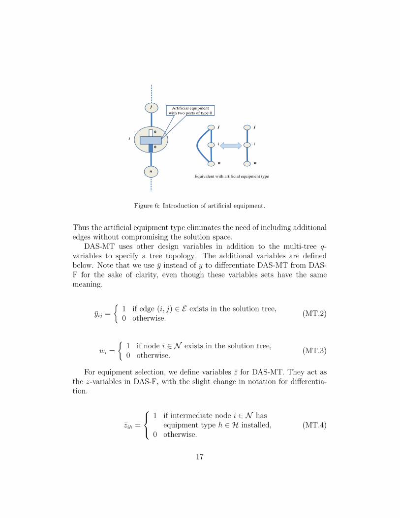
Besides the consideration of a type-0 outgoing port for every equipmenttype, we introduce an artificial equipment type. The equipment type has asingle type-0 output port, and, similar to the other equipment types, a type-0output port on the incoming side. The reason of introducing the artificialequipment type is similar to that for including the type-0 port. Namely, someintermediate nodes in the tree may have a degree of two, and for such nodes anoutput loss value is necessitated by the definition of the q-variables. Installingan artificial equipment, which corresponds to no real equipment selection,meets this requirement. The aspect is illustrated for node i in the exampleshown in Figure 6. Note that the use of artificial equipment can be avoidedhere, if edge (j, n) is present in the underlying graph. However, with such“shortcut” edges, the graph size becomes prohibitively high for optimization.

16

�

�

�

�

�

Artificial equipment

with two ports of type 0

�

�

�

�

�

�

Equivalent with artificial equipment type

Figure 6: Introduction of artificial equipment.

Thus the artificial equipment type eliminates the need of including additionaledges without compromising the solution space.

DAS-MT uses other design variables in addition to the multi-tree q-variables to specify a tree topology. The additional variables are definedbelow. Note that we use y instead of y to differentiate DAS-MT from DAS-F for the sake of clarity, even though these variables sets have the samemeaning.

yij =

{1 if edge (i, j) ∈ E exists in the solution tree,0 otherwise.

(MT.2)

wi =

{1 if node i ∈ N exists in the solution tree,0 otherwise.

(MT.3)

For equipment selection, we define variables z for DAS-MT. They act asthe z-variables in DAS-F, with the slight change in notation for differentia-tion.

zih =

1 if intermediate node i ∈ N has

equipment type h ∈ H installed,0 otherwise.

(MT.4)

17

The variables defined thus far do not indicate if (i, j) is in the path fromthe BS to an antenna t or not. This indication is necessary for power calcu-lation. To identify the paths from the BS, the following variables are used.

xtij =

1 if edge (i, j) ∈ E exists in the path

from the BS to antenna t ∈ T ,0 otherwise.

(MT.5)

Unlike xtij in DAS-F, xtij is defined for edges instead of arcs. As will beclear later on, the power of each antenna can be expressed without explicitlyspecifying which direction of an edge is used for the path from the BS. Thelast set of variables are continuous power variables. For DAS-MT, powervariables are required only for the BS and the antennas, as defined below.

pi = power of node i, i ∈ {s} ∪ T . (MT.6)

5.2. Constraints

Following the description style for DAS-F, the constraints for DAS-MTare grouped into four categories. The first three categories are defined fortopology design, equipment selection, and power calculation, respectively.The fourth category of constraints, referred to as path identification con-straints, is used to identify the edges forming the path from the BS to eachantenna, in order to facilitate power calculation.

• Topology design: The constraints for topology design in DAS-MTare provided below. Together they ensure the edges chosen indeedform a tree that connects all the leaf nodes (the BS and antennas) viaintermediate nodes. We remark that the number of constraint sets isnot as high as it may appear at a first glance, because many of themare special cases of others.

Constraints (MT.7) state a necessary condition of a tree topology,namely the number of edges is equal to the number of nodes minusone. By the two sets of constraints (MT.8) and (MT.9), the inclusionof any edge (i, j) ∈ E in the tree is possible only if both nodes i andj are part of the tree. Note that the BS and antennas must always bein the tree; this is ensured by constraints (MT.10). If an intermediatenode is used in the tree topology, then the node must be able to reach

18

both the BS with a type-0 port, as well as all the antennas with otherport types. These conditions are formulated in constraints (MT.11)and (MT.12).

∑(i,j)∈E

yi,j =∑

i∈N∪{s}∪T

wi − 1 (MT.7)

wi ≥ yij, ∀(i, j) ∈ E (MT.8)

wj ≥ yij, ∀(i, j) ∈ E (MT.9)

wi = 1, ∀i ∈ {s} ∪ T (MT.10)

wi =∑

j∈N∪{s}:(i,j)∈A

q0sij , ∀i ∈ N (MT.11)

wi =∑

j∈N∪T :(i,j)∈A

∑r∈R

qrtij , ∀i ∈ N , t ∈ T (MT.12)

ws =∑

j∈N :(j,s)∈A

q0sjs (MT.13)

wt =∑

j∈N :(j,t)∈A

∑r∈R:r 6=0

qrtjt , ∀t ∈ T (MT.14)

∑r∈R

qrkij +∑r∈R

qrkji = yij, ∀(i, j) ∈ E : i, j ∈ N , k ∈ {s} ∪ T

(MT.15)∑r∈R

qrjij = yij, ∀(i, j) ∈ E : i, j ∈ N (MT.16)∑r∈R

qriji = yij, ∀(i, j) ∈ E : i, j ∈ N (MT.17)

q0sij + q0sji = yij, ∀(i, j) ∈ E : i, j ∈ N (MT.18)∑r∈R

qrsjs = ysj, ∀(s, j) ∈ E (MT.19)

q0sjs = ysj, ∀(s, j) ∈ E (MT.20)∑r∈R,t∈T

qrtis = 0, ∀(i, s) ∈ A (MT.21)∑r∈R:r 6=0

qrtit = yit, ∀(i, t) ∈ E : t ∈ T (MT.22)

19

∑r∈R,k∈{s}∪T :k 6=t

qrkit = 0, ∀(i, t) ∈ A : t ∈ T (MT.23)

qrkij ≤ qrjij , ∀(i, j) ∈ A, r ∈ R, k ∈ {s} ∪ T(MT.24)

The BS and the set of antennas must be connected via intermediatenodes. Constraints (MT.13) model the condition that an intermedi-ate node is connected to the BS with a type-0 port, while constraints(MT.14) model the condition that for each antenna, there is an arcfrom one of the intermediate nodes connecting to it with a port typeother than type-0.

Constraints (MT.15) to (MT.23) form the bulk of conditions ensur-ing that the reachability specified by the q-variables are coherent witheach other to specify a common tree. These constrains consist in threegroups: (MT.15) to (MT.18) for edges between intermediate nodes,(MT.19) to (MT.21) for selecting an edge from the BS, and (MT.22)and (MT.23) for edges between the intermediate nodes and the anten-nas.

1. Consider first any edge (i, j) between intermediate nodes i ∈ Nand j ∈ N . If (i, j) is part of the tree topology (i.e., yij = 1), thenthe BS and all the antennas are reached in one of the directions(i, j) and (j, i) with one of the port types (possibly zero). This factis formulated by (MT.15). By (MT.16) and (MT.17), exactly oneport type is chosen for each of the two directions of an edge, if theedge is in the tree. For the source BS node s, type-0 port must beused in the direction towards it, as stated by constraints (MT.18).Constraints (MT.24) provide consistency in port selection. Thatis, if arc (i, j) has port type r associated, then this is the onlypossible port type to be used towards all leaves.

2. Next, consider edge selection towards some intermediate nodefrom the BS. By constraints (MT.19), if edge (s, j) ∈ E is selected,then there is one port type associated with arc (j, s). Furthermore,the port is of type-0, as ensured by (MT.20). As a leaf node, theBS is a termination point, thus arc (j, s) does not lead to the otherleaf nodes (i.e., the antennas). This fact is explicitly modeled byconstraints (MT.21).

20

3. The final sets of constraints (MT.22) and (MT.23) model thetopology conditions for edges between the intermediate nodes andthe antennas. Constraints (MT.22) ensure that if edge (i, t) witht ∈ T exists in the solution tree, then a port type other than type-0 must be associated with it in the direction from i to t. Similarto the source BS, the antennas are leaves and hence terminationpoints of the topology, and, therefore, an arc coming into an an-tenna does not lead further to any other leaf node, as formulatedin constraints (MT.23).

• Power equipment selection: Modeling power equipment selectionis relatively simple in DAS-MT. Two sets of constraints, as formulatedbelow, ensure equipment installation and the use of the equipment’sport types.

∑h∈H

zih = wi, ∀i ∈ N (MT.25)∑j∈{s}∪N∪T :(i,j)∈A

qrjij =∑h∈H

αrhzih, ∀i ∈ N , r ∈ R (MT.26)

An equipment type is selected for installation at an intermediate node,if and only if the node is in the tree. The condition is formulated withconstraints (MT.25). As was mentioned earlier, variable qrjij , (i, j) ∈A, r ∈ R has the effect of port selection over arc (i, j) at intermediatenode i. By taking the sum of the variables over all outgoing arcs for onespecific port type, as done in the left-hand side of (MT.26), we obtainthe number of ports of type r at node i. This has to be equal to thenumber of ports of the same type that are available on the equipmentselected for the node, as all the output ports of the installed equipmentshould be used. The equality is ensured by (MT.26).

• Path identification: In DAS-F, the path from the BS to every an-tenna is easily identified by the flow variables. For DAS-MT, the infor-mation is carried by the x-variables. Thus enabling power calculationrequires constraints identifying the paths connecting the BS to the an-tennas, i.e., to link the x-variables with the topology design. Here,path identification consists in knowing the edges of each path as well

21

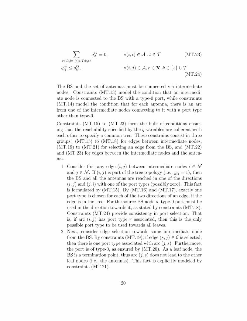
as the port types along the path. Two scenarios have to be accountedfor, as illustrated in the example in Figure 7 for arcs (i, j) and (i, k)and antenna t.

�

� �

�

�

�

� �

�

�

Flow towards the BS

Flow towards antenna

Figure 7: Illustration of path generation.

– Intermediate edge (i, j) is part of the path between the BS andantenna t. In this case, one of the two associated arcs (i, j) and(j, i) leads to t, and the opposite one leads to the BS. Withoutloss of generality, suppose t is reached via arc (i, j), see the leftpart of Figure 7. Thus

∑r∈R q

rtij = 1 and

∑r∈R q

rsij = 0. For arc

(j, i), we have q0sji = 1 since the arc has the direction towards theBS, and

∑r∈R q

rtji = 0.

– Intermediate edge (i, k) is not part of the path between the BS andantenna t. The scenario is shown in the right part of Figure 7,assuming without loss of generality that arc k reaches the BS viai. In this case, arc (k, i) will also lead to antenna t, meaningthat q0tki = 1 and q0ski = 1. The opposite arc (i, k) will obviouslylead to neither the BS nor antenna t, implying

∑r∈R q

rtik = 0 and∑

r∈R qrsik = 0.

Based on the above discussion, we introduce the following constraintsfor linking together the x-variables with the tree topology. For edgesbetween the intermediate nodes, the constraints consist of a numberof inequalities in order to achieve the desired effect of determining thevalues of the x-variables, whereas for the edges of the BS and antennas,the constraints can be formulated as equalities.

22

xtij ≥∑r∈R

qrtij −∑r∈R

qrsij , ∀(i, j) ∈ E : i, j ∈ N (MT.27)

xtij ≤∑r∈R

qrtij +∑r∈R

qrsij , ∀(i, j) ∈ E : i, j ∈ N (MT.28)

xtij ≥∑r∈R

qrtji −∑r∈R

qrsji , ∀(i, j) ∈ E : i, j ∈ N (MT.29)

xtij ≤∑r∈R

qrtji +∑r∈R

qrsji , ∀(i, j) ∈ E : i, j ∈ N (MT.30)

xtsj = ysj, ∀t ∈ T , (s, j) ∈ E (MT.31)

xtit = yit, ∀(i, t) ∈ E (MT.32)

Constraints (MT.27) and (MT.29) correspond to the first scenario dis-cussed above (see the left part of Figure 7). If the right-hand side of(MT.27) is one, then arc (i, j) is in the path from s to t, hence xtij mustbe one. Note that the constraints are defined over the edges. Therefore(MT.29) is needed to account for the case that the opposite arc is in thepath from s to t. Constraints (MT.28) and (MT.30) are formulated forthe second scenario (see the right part of Figure 7), where edge (i, j)is not in the path between s and t. In this case the right-hand sideis zero, forcing xtij to be zero as well. Finally, equalities (MT.31) and(MT.32) treats the edges between the BS and intermediate nodes, andthose between the intermediate nodes and the antennas.

• Power constraints: Power calculation at the antennas is enabled bycombining the x-variables that identify the paths from the BS and theq-variables that carry information of port type of the arcs in the tree.The set of constraints for power calculation is given below.

pt = ps −∑

(i,j)∈E

ξdijxtij −

∑(i,j)∈A,r∈R,i 6=s

rqrtij , ∀t ∈ T (MT.33)

The first sum in (MT.33),∑

(i,j)∈E ξdijxtij, represents the total cable loss

along the path from the BS to each antenna. The accumulated loss byequipment ports is given by

∑(i,j)∈A,r∈R,i 6=s rq

rtij . Note that in this sum,

23

qrtij = 1 does not necessarily mean (i, j) is on the path from s to t, as(i, j) can be as well on the path towards s, cf. Figure 7. In this case,however, the port is of type-0 (see the discussion of the constraints fortopology design), and hence does not have effect on power calculation.Unlike DAS-F, power calculation by (MT.33) does not require the useof any big-M parameter. Finally, the following inequalities, which areused in DAS-F as well, together formulate maximum allowed powerdeviation, i.e., |ptart − pt| ≤ pthrt .

pthrt ≥ ptart − pt, ∀t ∈ T (MT.34)

pthrt ≥ pt − ptart , ∀t ∈ T (MT.35)

5.3. Objective function

With the presence of y-variables in DAS-MT, expressing the objective ofminimizing the total cable length is simple. The function is provided below.

∑(i,j)∈E

dij yij (MT.36)

5.4. Model summary

Based on the previous discussions, formulation DAS-MT can be summa-rized as follows:

[DAS−MT] : min (MT.36)

s.t. (MT.7)− (MT.23), (MT.33), (MT.34), (MT.35)

In comparison to DAS-F, DAS-MT is much less straightforward to de-velop. This increased complexity in modeling does pay off. As will be shownby numerical results, DAS-MT scales much better than DAS-F in problemsolving.

6. Computational efficiency aspects and pre-processing

IB-DAS deployment optimization is very challenging even for small sce-narios. In this section, we discuss problem size reduction within the applica-tion context. Namely, real deployment of IB-DAS will follow to a large extent

24

engineering practice as well as the restriction posed by the deployment en-vironment. Thus it is reasonable to take these aspects into consideration forthe purpose of speeding up the optimization process.

6.1. Integrating the building structure into modeling

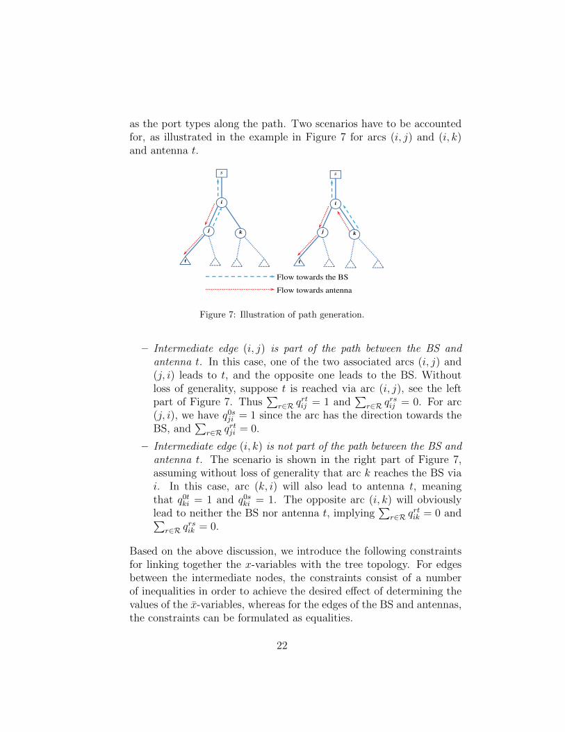
The computational effort for solving the IB-DAS deployment problemgrows rapidly in the size of the underlying graph. Without any restrictionon where cable connections can be set up, the edges of the intermediatenodes will form a complete graph. For real-life scenarios, however, this is notthe case, because the installation of cables and power equipments, similarto the deployment of other types of electrical infrastructure, will mainlyfollow the building structure and its internal layout to ease the installationas well as to makes it easier for future maintenance. Furthermore, as anemerging trend, IB-DAS is becoming an integrated part of new buildings’design and construction. Thus the cabling topology will be heavily correlatedwith building structure. Figure 8 shows a 3D view of one example floor of abuilding, along with a demonstrative cabling solution of IB-DAS. The cableinstallation follows well the building structure. In particular, the backbonecables go mainly along the corridors and pathways.

Building structure Cable installation

Figure 8: Illustration of cable installation.

As discussed above, we utilize building structure for reducing the problemsize of practical IB-DAS deployment. The candidate locations of the inter-mediate nodes for equipment installation are defined in such a way that theyfollow the pathways formed by floor layout and that equipment can be easilyinstalled. This pre-processing significantly reduces the number of edges tobe considered. An example is shown in Figure 9, with a total of 27 inter-mediate nodes serving as possible connection points to connect the BS to 11

25

antennas. As can be seen, the intermediate nodes give a strong indication ofcable installation. In fact, in this example, an underlying tree backbone canbe easily identified, though not all intermediate nodes necessarily are part ofthe optimal deployment and hence the topology optimization task remains.

�� �� �� �� ��� ��� ��� ��� ������

�

��

��

��

��

���

�

�

�� ������� �������

�� �����

(m)

(m)

Figure 9: Illustration of the backbone structure of 27 candidate intermediate nodes and11 antennas.

6.2. The use of artificial equipment type

Recall that the artificial equipment type for DAS-MT has two type-0ports, of which one is simply the opposite direction of the incoming port.The introduction of this equipment type allows for removing edges that canbe formed by a sequence of other and shorter edges, as illustrated in Figure 6.In fact, the idea applies also to DAS-F, by introducing an artificial equipmentwith one single type-0 port. The size reduction enables speeding up theoptimization process without compromising solution quality.

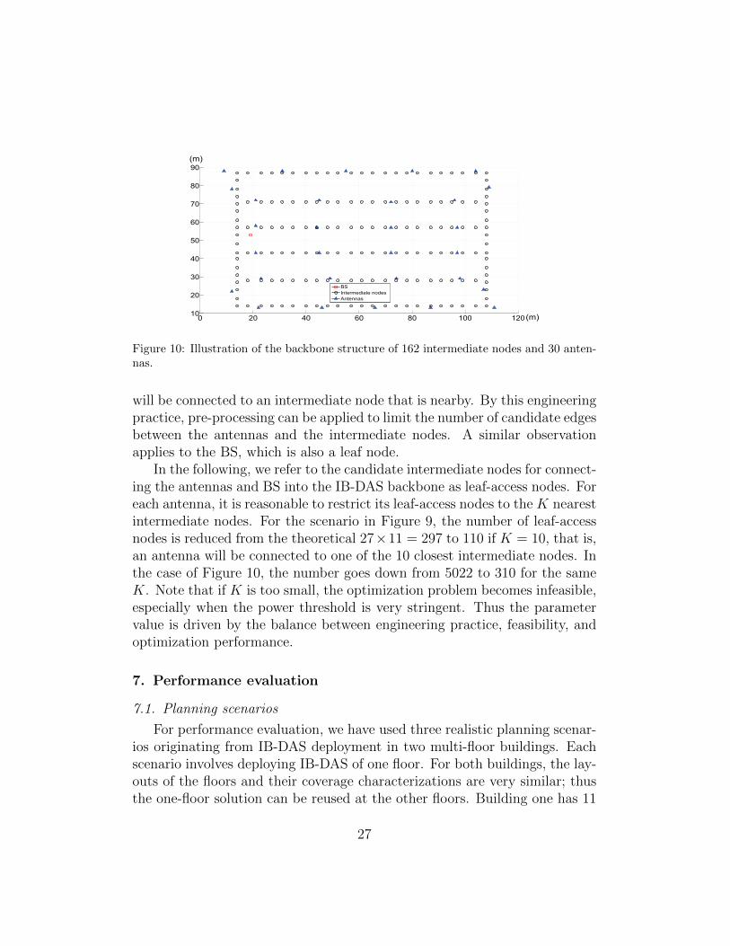
The size reduction via artificial equipment is significant. In the example ofFigure 9, the number of edges between the 27 intermediate nodes is reducedto 26, i.e., the underlying topology of the intermediate nodes is a spanningtree. A denser scenario with 162 intermediate nodes is shown in Figure 10.In this case, the number of edges of these nodes becomes around 170 afterthe reduction.

6.3. Reducing candidate connections for antennas

Even if connecting an antenna to a far-away intermediate node may bea good choice in theory (e.g., better power output), in practice the antenna

26

� �� �� �� �� ��� �����

��

��

��

��

��

�

��

�

�

�

�

������������������

��������

(m)

(m)

Figure 10: Illustration of the backbone structure of 162 intermediate nodes and 30 anten-nas.

will be connected to an intermediate node that is nearby. By this engineeringpractice, pre-processing can be applied to limit the number of candidate edgesbetween the antennas and the intermediate nodes. A similar observationapplies to the BS, which is also a leaf node.

In the following, we refer to the candidate intermediate nodes for connect-ing the antennas and BS into the IB-DAS backbone as leaf-access nodes. Foreach antenna, it is reasonable to restrict its leaf-access nodes to the K nearestintermediate nodes. For the scenario in Figure 9, the number of leaf-accessnodes is reduced from the theoretical 27×11 = 297 to 110 if K = 10, that is,an antenna will be connected to one of the 10 closest intermediate nodes. Inthe case of Figure 10, the number goes down from 5022 to 310 for the sameK. Note that if K is too small, the optimization problem becomes infeasible,especially when the power threshold is very stringent. Thus the parametervalue is driven by the balance between engineering practice, feasibility, andoptimization performance.

7. Performance evaluation

7.1. Planning scenarios

For performance evaluation, we have used three realistic planning scenar-ios originating from IB-DAS deployment in two multi-floor buildings. Eachscenario involves deploying IB-DAS of one floor. For both buildings, the lay-outs of the floors and their coverage characterizations are very similar; thusthe one-floor solution can be reused at the other floors. Building one has 11

27

antennas. For this building, two scenarios are defined, where the numbers ofcandidate intermediate nodes are 27 and 52, respectively. Building two has30 antennas. For this building, a scenario with 162 candidate intermediatenodes is defined. The antenna locations as well as the power targets havebeen derived from a radio access planning tool [21] for IB-DAS. For candidateintermediate nodes, the selection has followed the discussion in Section 6.

Building layout data have been pre-processed and integrated with themodeling process. The layouts of the first and last scenarios are illustratedin Figure 9 and Figure 10 of Section 6, respectively.

Table 1: A summary of the test scenarios.

Floor area (m2) 10000Number of candidate intermediate nodes 27/52/162

Number of antennas 11/11/30Cable loss per meter (dB) 0.0142Even power splitters (dB) (E1: 3.6, 3.6), (E2: 5.7, 5.7, 5.7)

Uneven power splitters (taps) (dB) (T1: 1.5, 6.15), (T2: 1.95, 5.15)(T3: 0.7, 10.15), (T4: 1.15, 7.15)

Antenna power target (dBm) 5Antenna power deviation threshold (dB) 1, 2, 3

A summary of the scenarios is provided in Table 1. Six equipment types,consisting of two types of power splitters (E1-E2 in the table) and four typesof taps (T1-T4 in the table), are available. The power loss settings of theseequipment types are given in Table 1. We apply three antenna power devi-ation thresholds (1, 2, and 3 dB), in order to gain insights on the trade-offbetween computational efficiency and the performance in meeting the powertarget. The optimization models DAS-F and DAS-MT have been solved us-ing the state-of-art integer programming solver Gurobi [22]. A limit of 10 hon the computing time is set for each scenario and parameter setting. We firstpresent results for the small scenario of 27 nodes, mainly for the purpose of acomparative study, demonstrating that the non-trivial DAS-MT formulationruns magnitudes faster than the simple formulation DAS-F in reaching theglobal optimum. Then we focus on the two large scenarios using formulationDAS-MT. After that, we provide a discussion of the time efficiency, and givesome general guidelines for practical IB-DAS deployment.

It is always desirable to have result comparison to baseline design so-lutions in performance evaluation. The IB-DAS problem that we consider,

28

however, represents an emerging engineering optimization topic for whichthere is no well-established algorithmic scheme in the literature. Indeed, thesimple IB-DAS design examples in [10] assume that the topology and antennaaccess are both given and fixed, when equipment selection is performed. Thisfollows the common practice of problem decomposition for wireless networkdeployment, namely to decompose the problem in question into sequentialsteps and optimize separately the planning variables of each step.

By the decomposition approach, a baseline scheme for the IB-DAS de-ployment problem is to first perform topology design, minimizing the totalcable length, followed by equipment selection. The first step amounts to solv-ing a degree-constrained minimum spanning tree (D-MST) problem. Notethat the presence of the maximum node degree is necessary, as there is a lim-ited maximum number of outgoing ports of the equipment types. As will beillustrated later in Section 7.3, the baseline topological design frequently failsin admitting equipment selection satisfying the power threshold. This resultfurther justifies mathematical modeling integrating the design decisions.

7.2. Performance results for small-scale scenario

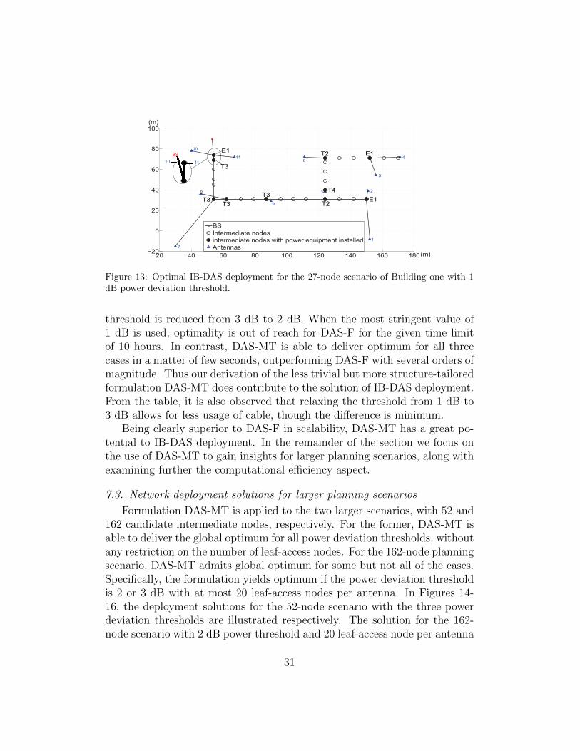
For the scenario of 27 intermediate nodes in Building one, the number ofleaf-access nodes K is set to four and then eight. The two values result inexactly the same optimum, indicating that the number of leaf-access nodes isnot critical in this case. Both DAS-F and DAS-MT admit global optimalitywithin the time limit for the cases with thresholds of 3 dB and 2 dB, whileonly DAS-MT is able to enable optimum for the case with 1 dB threshold.The optimal solutions for the three power deviation thresholds (3, 2, and 1dB) are shown in Figures 11-13, respectively. The filled black circles indicatethe locations of power equipments, and the label (e.g., E1) for each of themrepresents the equipment type (see also Table 1). One can observe thatalthough the solutions for various power deviation thresholds are similar toeach other, differences do occur for antenna connections close to the BS.Note that for two of the three cases, the BS is connected to its second closestintermediate node, as shown by the zoom-in illustration.

The performance results in terms of optimum value (i.e., minimum cablelength) and computing times for the case of four leaf-access nodes per antennaare summarized in Table 2. Notation “-” denotes that the time limit of 10h is exceeded. The performance figure for the setup of eight access nodesis similar. The computational time values in Table 2 reveal the tremendousdifference in the performance of the two formulations, and thereby highlight

29

20 40 60 80 100 120 140 160 180−20

0

20

40

60

80

100

1

23

4

5

6

7

8

9

10

11

BS

Intermediate nodes

intermediate nodes with power equipment installed

Antennas

(m)

(m)

10 11

BSE1

T3

T3

T3

T3

T2

T4

T2

E1

E1

Figure 11: Optimal IB-DAS deployment for the 27-node scenario of Building one with 2dB power deviation threshold.

20 40 60 80 100 120 140 160 180−20

0

20

40

60

80

100

1

23

4

5

6

7

8

9

10

11

BS

Intermediate nodes

intermediate nodes with power equipment installed

Antennas

(m)

(m)

T3

T3

T3

T4

T1

T2

T4

T1

E1

E1

Figure 12: Optimal IB-DAS deployment for the 27-node scenario of Building one with 3dB power deviation threshold.

Table 2: Performance results of the 27-node scenario with four leaf-access nodes per an-tenna.

Power deviation Optimum cable Computing time (seconds)threshold (dB) length (m) DAS-F DAS-MT

1 465 - 32 461 27704 33 457 123 1.7

the importance of optimization modeling to problem solving. Using DAS-F, the computing time jumps from two minutes to several hours, when the

30

20 40 60 80 100 120 140 160 180−20

0

20

40

60

80

100

1

23

4

5

6

7

8

9

10

11

BS

Intermediate nodes

intermediate nodes with power equipment installed

Antennas

(m)

(m)

10 11

BSE1

T3

T3T3

T3

T2

T4

T2

E1

E1

Figure 13: Optimal IB-DAS deployment for the 27-node scenario of Building one with 1dB power deviation threshold.

threshold is reduced from 3 dB to 2 dB. When the most stringent value of1 dB is used, optimality is out of reach for DAS-F for the given time limitof 10 hours. In contrast, DAS-MT is able to deliver optimum for all threecases in a matter of few seconds, outperforming DAS-F with several orders ofmagnitude. Thus our derivation of the less trivial but more structure-tailoredformulation DAS-MT does contribute to the solution of IB-DAS deployment.From the table, it is also observed that relaxing the threshold from 1 dB to3 dB allows for less usage of cable, though the difference is minimum.

Being clearly superior to DAS-F in scalability, DAS-MT has a great po-tential to IB-DAS deployment. In the remainder of the section we focus onthe use of DAS-MT to gain insights for larger planning scenarios, along withexamining further the computational efficiency aspect.

7.3. Network deployment solutions for larger planning scenarios

Formulation DAS-MT is applied to the two larger scenarios, with 52 and162 candidate intermediate nodes, respectively. For the former, DAS-MT isable to deliver the global optimum for all power deviation thresholds, withoutany restriction on the number of leaf-access nodes. For the 162-node planningscenario, DAS-MT admits global optimum for some but not all of the cases.Specifically, the formulation yields optimum if the power deviation thresholdis 2 or 3 dB with at most 20 leaf-access nodes per antenna. In Figures 14-16, the deployment solutions for the 52-node scenario with the three powerdeviation thresholds are illustrated respectively. The solution for the 162-node scenario with 2 dB power threshold and 20 leaf-access node per antenna

31

is shown in Figure 17.

20 40 60 80 100 120 140 160 180−20

0

20

40

60

80

100

1

23

4

5

6

7

8

9

10

11

BS

Intermediate nodes

intermediate nodes with power equipment installed

Antennas

(m)

(m)

10

11

BS

8

7

E1

T3

T3T3

T3T4

T2

T1 E1

E1

Figure 14: Optimal IB-DAS deployment the 52-node scenario with 1 dB power deviationthreshold.

20 40 60 80 100 120 140 160 180−20

0

20

40

60

80

100

1

23

4

5

6

7

8

9

10

11

BS

Intermediate nodes

intermediate nodes with power equipment installed

Antennas

(m)

(m)

10

11

BSE1

T3

T3

T3

T3T4

T2

T1 E1

E1

Figure 15: Optimal IB-DAS deployment the 52-node scenario with 2 dB power deviationthreshold.

As can be seen from the 52-node scenario, varying the power deviationthreshold leads to slightly different topology solutions and power equipmenttype selections. There is clear coupling between the threshold and topology,namely the selection of leaf-access nodes becomes less intuitive for smallerthreshold in order to satisfy the threshold constraint. An example is an-tenna eight. This antenna is connected to its closest intermediate node whenthe threshold is over 2 dB, whereas for the 1 dB threshold an intermediatenode being further away is chosen, For the 162-node scenario, the underlying

32

20 40 60 80 100 120 140 160 180−20

0

20

40

60

80

100

1

23

4

5

6

7

8

9

10

11

BS

Intermediate nodes

intermediate nodes with power equipment installed

Antennas

(m)

(m)

T3T3

T3T3

T4T4

T2

T1 E1

E1

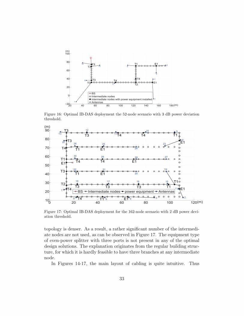
Figure 16: Optimal IB-DAS deployment the 52-node scenario with 3 dB power deviationthreshold.

0 20 40 60 80 100 12010

20

30

40

50

60

70

80

90

1

23456

7

8

910

11

12

13

14

15161718

19

20

2122

23

24

2526

27282930

BS Intermediate nodes power equipment Antennas

(m)

(m)

E1

T3

T3

T4

T1

T3

T2

T4

T1

T4

T1

T3

T4

T3 T4 T4

E1

T4 E1

E1

T3 T3

T1 E1

T1

E1

T1

T1

E1

Figure 17: Optimal IB-DAS deployment for the 162-node scenario with 2 dB power devi-ation threshold.

topology is denser. As a result, a rather significant number of the intermedi-ate nodes are not used, as can be observed in Figure 17. The equipment typeof even-power splitter with three ports is not present in any of the optimaldesign solutions. The explanation originates from the regular building struc-ture, for which it is hardly feasible to have three branches at any intermediatenode.

In Figures 14-17, the main layout of cabling is quite intuitive. Thus

33

the solutions may appear to submit to a manual approach of simply settingup the design by hand. However, two aspects prohibit the use of such anapproach. First, for a large-scale scenario, determining the optimal linksconnecting the intermediate nodes is not simple. For example, in Figure 17two cables terminate at antennas 20 and 24, respectively, even if there doexists additional “downstream” antennas to be connected. In contrast, thecable in the middle goes all the way to antenna 27. This optimal combinationof connections does not follow directly from manual planning. Second andmore importantly, the approach is very prone to errors in selecting antennaaccess, i.e., to which intermediate node each antenna should be connected,because in many cases the optimal choice is not the intuitive one. Examplesinclude the zoomed-in areas in Figures 14-15, and antennas 19 and 23 inFigure 17. Note also that the power output at an antenna depends on theequipment selection along the entire path to the BS. Thus the performanceis a joint effect of topology design and equipment selection, and decouplingthese decisions does not result in a feasible solution scheme.

In Figures 18-19, we provide the distribution of the antenna power for thedesign solutions. The labels on the x-axis represent antenna indices. The y-axis is the antenna power, with a target value of 5 dBm for all antennas.From the figures, one observes that the proportion of antennas having themaximum allowed deviation is about 10%, hence most of the power deviationsare strictly within the threshold. As expected, the power deviation tends togrow when the threshold increases. For the 52-node scenario, the averagepower deviations over the antennas are 0.58, 0.83, and 1.74 dB for thresholdsof 1, 2, and 3 dB, respectively. For the 162-node scenario, the average valueis 1.05 for the 2 dB threshold. Thus the overall deviation is about half of thespecified threshold value.

�

�

�

�

�

�

�

� � � � � � � � � ��

�� ����������������

�� ����������

����� ��������

����� ��������

����� ��������

Figure 18: Antenna power distribution for the 52-node scenario.

34

�

���

�

���

�

���

�

� � � � � � � �� �� �� �� �� �� �� �� � � �� �� �� �� �� �� �� �� � � ��

������������� ��

������������� �� ����������

Figure 19: Antenna power distribution for the 162-node scenario with threshold 2 dB.

7.4. Computational performance aspects

From a performance viewpoint, several aspects are of significance in com-putational optimization of IB-DAS deployment. First, to approach globaloptimality, the choice of optimization formulation is crucial, as demonstratedby the comparative study in Section 7.2. Second, the problem size, in partic-ular the number of edges has high impact on the computational requirement.Utilizing the backbone structure derived via building survey, as was illus-trated in Section 6, is a key step towards computational efficiency. Thenumber of edges is also highly dependent on the number of leaf-access nodes(i.e., parameter K) defined for each antenna. Reducing the number speedsup the optimization process but potentially has a negative impact on thetotal cable length or even causes infeasibility. Third, decreasing the powerdeviation threshold will drive the solution closer to the power target. At thesame time, it becomes harder to solve the optimization problem, which maybe infeasible if the threshold is too small.

In Table 3, we summarize the performance results of solving the IB-DAS deployment problem for the three scenarios by DAS-MT for variouscombinations of K and power deviation thresholds. In the table, “-” indicatesthat no solution is obtained within the time limit.

As can be observed from the table, the graph size in the number of edgesgrows with respect to the number of leaf-access nodes, and the amount ofgrowth increases by scenario size. For the 27-node scenario, setting K = 20instead of 10 gives a moderate size increase. If the restriction is waivedcompletely (i.e., an antenna can be connected to any of the intermediatenodes), the number of edges is more than doubled. For the largest scenarioof 162 nodes, increasing K from 10 and 20 brings the number of edges from471 to 781. If no restriction is imposed, the number jumps to above 5000.The increase in graph size directly translates to the computational effort,particularly if the power deviation threshold is small. Consider the threshold

35

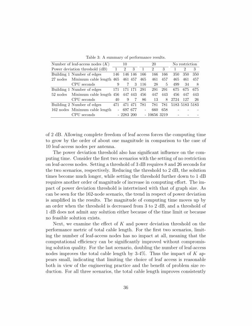
Table 3: A summary of performance results.

Number of leaf-access nodes (K) 10 20 No restrictionPower deviation threshold (dB) 1 2 3 1 2 3 1 2 3

Building 1 Number of edges 146 146 146 166 166 166 350 350 35027 nodes Minimum cable length 465 461 457 465 461 457 465 461 457

CPU seconds 9 7 3 116 28 5 499 34 8

Building 1 Number of edges 171 171 171 291 291 291 675 675 67552 nodes Minimum cable length 456 447 443 456 447 443 456 447 443

CPU seconds 40 9 7 86 13 8 2724 127 26

Building 2 Number of edges 471 471 471 781 781 781 5183 5183 5183162 nodes Minimum cable length - 697 677 - 660 658 - - -

CPU seconds - 2283 200 - 10656 3219 - - -

of 2 dB. Allowing complete freedom of leaf access forces the computing timeto grow by the order of about one magnitude in comparison to the case of10 leaf-access nodes per antenna.

The power deviation threshold also has significant influence on the com-puting time. Consider the first two scenarios with the setting of no restrictionon leaf-access nodes. Setting a threshold of 3 dB requires 8 and 26 seconds forthe two scenarios, respectively. Reducing the threshold to 2 dB, the solutiontimes become much longer, while setting the threshold further down to 1 dBrequires another order of magnitude of increase in computing effort. The im-pact of power deviation threshold is intertwined with that of graph size. Ascan be seen for the 162-node scenario, the trend in respect of power deviationis amplified in the results. The magnitude of computing time moves up byan order when the threshold is decreased from 3 to 2 dB, and a threshold of1 dB does not admit any solution either because of the time limit or becauseno feasible solution exists.

Next, we examine the effect of K and power deviation threshold on theperformance metric of total cable length. For the first two scenarios, limit-ing the number of leaf-access nodes has no impact at all, meaning that thecomputational efficiency can be significantly improved without compromis-ing solution quality. For the last scenario, doubling the number of leaf-accessnodes improves the total cable length by 3-4%. Thus the impact of K ap-pears small, indicating that limiting the choice of leaf access is reasonableboth in view of the engineering practice and the benefit of problem size re-duction. For all three scenarios, the total cable length improves consistently

36

by relaxing the power deviation constraint. However, the difference is verymoderate. Thus setting the power deviation threshold shall be based on theimportance of meeting the power target and computational aspects, ratherthan its impact on the optimization objective.

In Table 3, there are a number of cases for which no solution is obtainedfor the 162-node scenario. For the threshold values of 2 and 3 dB, the lack ofsolution is clearly caused by problem size, as the problem could be success-fully solved by restricting the number of leaf-access nodes. Note that anysolution found with restricted leaf access (K = 10 and K = 20) is also avalid design for the same scenario with no restriction on K. Therefore feasi-ble though not necessarily optimal solutions are indeed available for the twothresholds under column ’No restriction’ in Table 3. For the most stringentthreshold of 1 dB, the reason of no solution in the table could be probleminfeasibility, namely the solution space is in fact empty.

From the results and discussions, setting the number of leaf-access nodesas well as the power deviation threshold are of high importance in IB-DASplanning. For a specific planning case, a number of computations may beperformed in order to balance the computation and performance.

Table 4: Performance results of the baseline design.

Scenarios Cable Minimum achievablelength (m) power deviation (dB)

Building 1, 27 nodes 457 2.31Building 1, 52 nodes 443 2.31Building 2, 162 nodes 657 3.35

In Table 4, we report the performance results of the baseline designscheme described in Section 7.1, namely, to decompose the problem into twosequential stages of topology optimization and equipment selection, respec-tively. The topology is derived from solving degree-constrained MST. For thegiven D-MST solution, we solve the equipment selection problem, with thecost function being the power deviation from the target. Thus the optimumvalue is the minimum achievable power deviation. If the value is within theinterval for the threshold, equipment selection is feasible and the D-MSTtopology is in fact globally optimal, otherwise the scheme fails. For the firsttwo scenarios in Building one, the baseline topology admits equipment se-lection for the threshold of 3 dB, and hence the topology solutions coincides

37

with the corresponding ones in Table 3. When the threshold decreases, how-ever, no feasible equipment selection exists for the baseline topology. For thelast scenario, the baseline topology fails, even for the largest power deviationthreshold. The results reveal that topology design is strongly intertwinedwith equipment selection in determining the overall performance, demon-strating the advantage of mathematical model that takes a global view ofthe problem.

8. Conclusions

By bringing radio access closer to the end users, IB-DAS is a promisingsolution for coverage and capacity for in-building mobile broadband. In thispaper, we have studied optimization of passive IB-DAS deployment. Theresulting optimization problem is very challenging. Topology design andequipment installation, driven by the cable cost and the power targets of theantennas, are tightly intertwined in the optimization process. We have takenan integer programming approach with emphasis on mathematical modeling.Two types of models, DAS-F and DAS-MT, have been developed. DAS-F,based on the widely used concept of network flows, is straightforward butproven to be useful only for small planning scenarios. DAS-MT uses theconcept of embedding multiple trees into a common tree. The formulationis more complicated than DAS-F, but exhibits high scalability. In addition,pre-processing techniques, ranging from integrating building structure to thenotion of artificial equipment, have been developed for improving computa-tional efficiency.

The numerical results demonstrate that the solution approach of modelingand mathematical programming is capable of approaching global optimalitywith reasonable computing effort for planning scenarios of practical rele-vance. Our computational study also sheds light on the trade-offs betweenoptimality, computational efficiency, and network performance. As a futurework, fast heuristics that are able to finding feasible solutions to very largescale IB-DAS deployment call for investigation, within which the results ofthe current paper effectively serve the purpose of benchmarking in perfor-mance evaluation. Algorithms that target determining problem feasibility forgiven power deviation threshold form another line of forthcoming research.Moreover, we remark that the DAS deployment problem considered in thecurrent paper is defined for given antenna locations and candidate interme-diate nodes, though for the latter the optimization process has to determine

38

which will actually be used in a design solution. Even with the locationsgiven, approaching global optimum is challenging for large scale cases, ascan be observed from the computational results. Extending the problem set-ting, in particular to include antenna location in the optimization process,is of practical interest, and solution approaches for the joint optimizationproblem form an important line of future work.

Acknowledgment

We would like to thank the anonymous reviewers for their valuable com-ments and suggestions. The work has been partially supported by the EL-LIIT research excellence center of Sweden, CENIIT of Linkoping University,Sweden, and the EC FP7 Marie Curie Programme.

References

[1] Nokia Siemens Networks, ”In Building Solutions Executive Summary,”2011.

[2] D. Hong, S. Choi, and J. Cho, “Coverage and capacity analysis forthe multi-layer CDMA macro/indoor-picocells,” in IEEE InternationalConference on Communications (ICC’99), vol. 1, pp. 354–358, 1999.

[3] J. Perez-Rornero, O. Salient, and R. Agusti, “On the capacity degrada-tion in WCDMA uplink/downlink due to indoor traffic,” in IEEE 60thVehicular Technology Conference (VTC2004-Fall), vol. 2, pp. 856–859,2004.

[4] K. Hiltunen, B. Olin, and M. Lundevall, “Using dedicated in-buildingsystems to improve HSDPA indoor coverage and capacity,” in IEEE 61stVehicular Technology Conference (VTC2005-Spring), vol. 4, pp. 2379–2383, 2005.

[5] B. Song, R. Cruz, and B. Rao, “Downlink optimization of indoor wire-less networks using multiple antenna systems,” in 23rd Annual JointConference of the IEEE Computer and Communications Societies (IN-FOCOM’04), vol. 4, pp. 2778–2789, 2004.

[6] H. Beijner, “The importance of in-building solutions in third generationnetworks,” Ericsson Review, 2004.

39

[7] J. Borkowski, J. Niemela, T. Isotalo, P. Lahdekorpi, and J. Lempiainen,“Utilization of an indoor DAS for repeater deployment in WCDMA,” inIEEE 63rd Vehicular Technology Conference (VTC2006-Spring), vol. 3,pp. 1112–1116, 2006.

[8] L. Chen, D. Yuan, H. Song, and J. Zhang, “Mathematical Modeling forOptimal Deployment of In-Building Distributed Antenna Systems,” inthe first International Conference on Communications in China (IEEE-ICCC ), pp. 786–791 2012.

[9] “The DAS forum.” www.thedasforum.org

[10] M. Tolstrup, Indoor Radio Planning, A Practical Guide for GSM, DCS,UMTS and HSPA. John Wiley & Sons, Ltd, 2008.

[11] M. R. Garey and D. S. Johnson, Computers and Intractability: A Guideto the Theory of NP-Completeness, W. H. Freeman, 1979.

[12] R. Rardin and L. Wolsey, “Valid inequalities and projecting the multi-commodity extended formulation for uncapacitated fixed charge networkflow problems,” Universite catholique de Louvain, Center for OperationsResearch and Econometrics (CORE), 1990.

[13] D. Bienstock and O. Gunluk, “Capacitated network design – polyhedralstructure and computation,” Informs Journal on Computing, vol. 8, pp.243–259, 1994.

[14] J. Hellstrand, T. Larsson, and A. Migdalas, “A characterization of theuncapacitated network design polytope,” Operations Research Letters,vol. 12, pp. 159–163, 1992.

[15] P. Belotti, F. Malucelli, and L. Brunetta, “Multicommodity networkdesign with discrete node costs,” Networks, vol. 49, pp. 90–99, 2007.

[16] D. Yuan, J. Bauer, and D. Haugland, “Minimum-energy broadcast andmulticast in wireless networks: An integer programming approach andimproved heuristic algorithms,” Ad Hoc Networks, vol. 6, pp. 696–717,2008.

[17] J. Bauer, D. Haugland, and D. Yuan, “Analysis and computationalstudy of several integer programming formulations for minimum-energy

40

multicasting in wireless ad hoc networks,” Networks, vol. 52, pp. 57–68,2008.

[18] M. Pioro and D. Medhi, Routing, Flow, and Capacity Design in Com-munication and Computer Networks, Morgan Kaufmann Publishers,2004.

[19] B. N. Khoury, P. M. Pardalos, and D. Hearn, “Equivalent formulationsfor the steiner problem in graphs,” D. Z. Du et al, (eds.), NetworkOptimization Problems, pp. 111–124, 1993.

[20] T. Polzin and S. V. Daneshmand, “A comparison of steiner tree relax-ations,” Discrete Applied Mathematics, vol. 112, pp. 241–261, 2001.

[21] RANPLAN iBuildNet R©, RANPLAN. www.ranplan.co.uk

[22] Gurobi solver, Gurobi Optimization. www.gurobi.com

41