Heat and fluid flow simulations for tomorrow’s energies JP Chabard Sept 2009.

HAL Id: tel-01646867https://tel.archives-ouvertes.fr/tel-01646867
Submitted on 19 Dec 2017
HAL is a multi-disciplinary open accessarchive for the deposit and dissemination of sci-entific research documents, whether they are pub-lished or not. The documents may come fromteaching and research institutions in France orabroad, or from public or private research centers.
L’archive ouverte pluridisciplinaire HAL, estdestinée au dépôt et à la diffusion de documentsscientifiques de niveau recherche, publiés ou non,émanant des établissements d’enseignement et derecherche français ou étrangers, des laboratoirespublics ou privés.
Mathematical modeling, analysis and simulations forfluid mechanics and their relevance to in silico medicine
Marcela Szopos
To cite this version:Marcela Szopos. Mathematical modeling, analysis and simulations for fluid mechanics and theirrelevance to in silico medicine. Analysis of PDEs [math.AP]. Université de Strasbourg, IRMA UMR7501, 2017. �tel-01646867�

Institut de RechercheMathématique Avancée
INSTITUT DERECHERCHE
MATHÉMATIQUEAVANCÉE
UMR 7501
Strasbourg
www-irma.u-strasbg.fr
Habilitation à diriger des recherches
Université de StrasbourgSpécialité MATHÉMATIQUES APPLIQUÉES
Marcela Szopos
Mathematical modeling, analysis and simulations for fluid mechanics and their relevance to in silico
medicine
Soutenue le 1 décembre 2017devant la commission d’examen
Dominique Chapelle, examinateurLuca Formaggia, rapporteur
Philippe Helluy, garantYvon Maday, examinateur
Kent-Andre Mardal, rapporteurSébastien Martin, rapporteur
Christophe Prud’homme, examinateurStéphanie Salmon, examinateur


Contents
Remerciements – Acknowledgments iii
Preambule 1
Introduction 5
1 Three-dimensional models, analysis and efficient simulations for fluid equations.Applications to computational hemodynamics in the cerebral network 9
1.1 Mathematical modeling of blood flow in the cerebral venous system . . . . . . . . . . 9
1.1.1 A new three-dimensional model for large cerebral veins . . . . . . . . . . . . . 10
1.1.2 Numerical results and discussion . . . . . . . . . . . . . . . . . . . . . . . . . 12
1.2 A novel formulation of the Stokes system involving pressure boundary conditions . . 14
1.2.1 General framework and the Lagrange multiplier formulation . . . . . . . . . . 15
1.2.2 Numerical results and applications . . . . . . . . . . . . . . . . . . . . . . . . 18
1.3 Influence of different modeling assumptions . . . . . . . . . . . . . . . . . . . . . . . 20
1.3.1 Sensitivity analysis framework . . . . . . . . . . . . . . . . . . . . . . . . . . 20
1.3.2 Numerical results and discussion . . . . . . . . . . . . . . . . . . . . . . . . . 22
1.4 Large-scale blood flow simulations and validation . . . . . . . . . . . . . . . . . . . . 24
1.4.1 Computational framework . . . . . . . . . . . . . . . . . . . . . . . . . . . . . 24
1.4.2 The FDA benchmark nozzle model . . . . . . . . . . . . . . . . . . . . . . . . 25
1.5 An open-source framework to generate virtual MRA images from real MRA images . 28
1.6 Conclusions and outlook . . . . . . . . . . . . . . . . . . . . . . . . . . . . . . . . . . 29
2 Reduced and multiscale mathematical and computational models for biofluids.Applications to the study of the coupled eye-cerebral system 33
2.1 Design and development of a lumped model for the coupled eye-cerebral system . . . 34
2.1.1 Construction of the model . . . . . . . . . . . . . . . . . . . . . . . . . . . . . 35
2.1.2 Microgravity conditions modeling and numerical results . . . . . . . . . . . . 40
2.2 A zoom on mathematical models for the aqueous humor . . . . . . . . . . . . . . . . 42
2.2.1 Modeling the intraocular pressure under uncertainty . . . . . . . . . . . . . . 43
2.2.2 Modeling the coupled dynamics of ocular blood flow and aqueous humor . . . 45
2.3 A new algorithm for the numerical solving of coupled distributed–0d problems . . . 48
2.3.1 Description of the coupled Stokes–0d problem . . . . . . . . . . . . . . . . . . 49
2.3.2 First-order splitting algorithm for the time discretization of the coupled prob-lem and stability analysis . . . . . . . . . . . . . . . . . . . . . . . . . . . . . 52
2.3.3 Numerical results and discussion . . . . . . . . . . . . . . . . . . . . . . . . . 53
2.4 Conclusions and outlook . . . . . . . . . . . . . . . . . . . . . . . . . . . . . . . . . . 56
i

ii CONTENTS
3 Numerical strategies for coupled fluid-structure problems. Applications to mul-tiphysics computational models in biology and medicine 593.1 Computational modeling of blood flow in the aorta . . . . . . . . . . . . . . . . . . . 59
3.1.1 Mathematical model and numerical approach . . . . . . . . . . . . . . . . . . 603.1.2 Numerical results and clinical applications . . . . . . . . . . . . . . . . . . . . 62
3.2 Discretization in time in simulations of particulate flows . . . . . . . . . . . . . . . . 663.2.1 Dense fluid-particle flows and difficulties arising in their simulations . . . . . 663.2.2 A model ordinary differential equation with lubrication forces . . . . . . . . . 67
3.3 Conclusions and outlook . . . . . . . . . . . . . . . . . . . . . . . . . . . . . . . . . . 71
References of the author 73
Other references 77

Remerciements – Acknowledgments
Je suis tres reconnaissante envers Sebastien Martin d’avoir accepte d’etre rapporteur de cememoire. Je le remercie du temps qu’il a consacre a la lecture du manuscrit et je suis tres honoreede l’interet qu’il a porte a mes travaux. I was very honored when Luca Formaggia and Kent-AndreMardal accepted to be reviewers of this Habilitation. I am very grateful for all the interestingremarks, questions and insights they provided.
C’est egalement avec plaisir que j’exprime mes vifs remerciements a Dominique Chapelle, PhilippeHelluy, Yvon Maday, Christophe Prud’homme et Stephanie Salmon. Je suis tres heureuse qu’ilsaient accepte de faire partie de mon jury et de donner leur avis constructif d’experts, malgre leurstres nombreuses obligations. Merci a Philippe d’avoir accepte d’etre le garant de cette habilitationet a Christophe pour nos innombrables echanges autour de Cemosis, Feel++, Eye2Brain et pleind’autres projets.
Je profite de cette occasion pour remercier chaleureusement tous mes collaborateurs, car tra-vailler a leurs cotes est tres enrichissant, tant d’un point de vue scientifique, que d’un point de vuehumain. En particulier, un grand merci aux relecteurs attentifs, qui ont contribue a l’ameliorationde ce document. Je pense egalement a tous les membres du projet ANR VIVABRAIN : que dechemin parcouru depuis les discussions avec Stephanie Salmon, Nicolas Passat et Olivier Genevauxautour d’un sujet de M2 et les resultats d’aujourd’hui. A special thanks to the Italian wing, inparticular to Giovanna Guidoboni and Riccardo Sacco: I am very grateful for all fruitful discussionsin Strasbourg, Milan or accross the Atlantic, that contributed to my work in uncountable ways. Iwould also like to thank Silvia Bertoluzza, for her expertise in all the topics we explored together.Plus generalement, mes remerciements vont vers tous les collegues avec qui j’ai pris beaucoup deplaisir a discuter des multiples facettes de notre activite d’enseignants-chercheurs, lors des echangesdans les conferences, seminaires, groupes de travail, etc. Je ne voudrais par terminer sans parlerdu CEMRACS (Centre d’Ete Mathematique de Recherche Avancee en Calcul Scientifique), lieuprivilegie de rencontres et de discussions autour des mathematiques. Je suis fort redevable pourtoutes les occasions ou j’ai pu beneficier de cet environnement exceptionnel et j’ai notamment unepensee pour mes co-organisateurs de l’edition 2015 : merci a Emmanuel Frenod, Emmanuel Maıtre,Antoine Rousseau et Stephanie Salmon pour cette belle aventure scientifique et humaine.
A l’Universite de Strasbourg, comme a l’Universite Paul Sabatier auparavant, j’ai eu la chancede profiter d’un cadre de travail tres favorable et d’une ambiance amicale. Que tous mes colleguestrouvent ici ma sincere gratitude. Ces remerciements vont tout autant aux equipes de soutien admi-nistratif et informatique, qui par l’efficacite et la qualite de leur travail, nous aident quotidiennement.
Enfin, je ne saurai jamais trouver les bons mots pour remercier tous ceux qui, avec beaucoup degenerosite et d’amour, m’ont aidee.
iii

iv

Preambule
Ce manuscrit rassemble mes contributions portant sur le developpement de nouvelles methodesmathematiques et numeriques pour l’analyse des ecoulements biologiques, consideres comme desphenomenes complexes multi-physiques et multi-echelles. La description des mecanismes sous-jacents decoule des principes de base de la mecanique des fluides et se traduit dans des systemesd’equations aux derivees partielles ou d’equations differentielles. L’objectif global de ce travail estl’etude de ces equations aux niveaux continu et discret et de leur couplage, ainsi que la mise en placed’un environnement de calcul permettant l’implementation fiable et efficace des differentes methodesnumeriques proposees pour approcher les solutions de ces problemes. Les simulations numeriquesainsi developpees prennent en compte des geometries realistes et une validation detaillee est pro-posee a travers des comparaisons avec des donnees experimentales, en vue de leur application a desquestions biomedicales specifiques.
L’approche in silico, consistant a combiner la modelisation basee sur des donnees et la modelisa-tion fondee sur les lois de la physique, dans le meme environnement de calcul, est devenue deplus en plus populaire dans le domaine des sciences de la vie ces dernieres annees et a motive ledeveloppement de nouveaux concepts mathematiques et numeriques. Malgre des avancees signi-ficatives dans la modelisation in silico de la physiologie humaine, l’etude de la dynamique com-plexe qui regit l’interaction entre differents fluides dans le corps humain suscite encore des ques-tions extremement difficiles. La description des fluides biologiques fait intervenir une large gammed’echelles spatiales et temporelles, entre le niveau moleculaire et celui des reseaux de quelques metres,avec une duree qui peut aller d’une seconde pour le cycle cardiaque a plusieurs dizaines d’anneespour une vie. La dynamique de ces fluides est influencee par l’interaction avec les tissus environ-nants, d’ou la necessite d’une approche multi-physique dans la modelisation. La representationgeometrique est tres complexe et peu de donnees realistes sont disponibles. En outre, dans lesetudes experimentales, de nombreux facteurs entrent en jeu et il est difficile d’isoler l’effet de chaquecontribution sur les caracteristiques de l’ecoulement. Dans cette direction, l’analyse statistique of-fre de nombreuses techniques pour aider a identifier des correlations entre les donnees, mais lacomprehension des relations de cause a effet a travers ces methodes reste limitee. Dans cette per-spective, la modelisation mathematique et numerique, basee sur les principes fondamentaux de laphysique et adaptee a un cadre biologique, peut aider a identifier des relations de cause a effet dansl’action conjuguee de multiples facteurs et ainsi ameliorer notre comprehension de ces phenomenescomplexes ; bien evidemment, cette analyse est amenee a se developper en synergie avec d’autresapproches.
Afin de mieux comprendre certaines difficultes rencontrees dans cette etude, il nous paraıt im-portant d’aborder a ce stade la question suivante : quelles sont les differences entre la modelisationdes fluides biologiques et celle des fluides “classiques” ? Compares a des fluides “classiques”, cesfluides remplissent des fonctions biologiques essentielles (par exemple le transport de nutriments et
1

2
d’oxygene, l’interaction avec les cellules environnantes), qui doivent etre prises en compte dans unmodele mathematique. Contrairement aux fluides “inertes”, leurs proprietes changent au cours dutemps, comme consequence de differents processus biologiques lies a l’age, a la maladie, etc. De nom-breux defis sont engendres par leur etude in vivo, car la plupart du temps, les fluides biologiques sontdifficilement accessibles dans leur milieu naturel ; en outre, ils montrent souvent des proprietes et descomportements differents lorsqu’ils sont examines in vitro ou in vivo. Par consequent, l’extensiondes theories classiques de la mecanique des fluides et de l’approche mathematique correspondantea l’etude des systemes biologiques souleve de nombreuses questions et represente actuellement undomaine de recherche tres actif.
Tous ces aspects conduisent a : (i) de nombreuses difficultes liees a la derivation d’un modelemathematique pertinent et bien pose a partir de la litterature biologique et clinique ; (ii) un be-soin important de developper de nouvelles approches theoriques et methodes numeriques ; (iii)une necessite croissante de concevoir et de mettre en œuvre un environnement de calcul flexible etefficace ; (iv) des efforts de recherche importants dedies a la verification, la validation et la priseen compte des incertitudes. Ces aspects sont cruciaux pour garantir que le modele et ses solutionsnumeriques sont significatifs du point de vue biomedical, permettant ainsi l’utilisation du cadreresultant comme un laboratoire virtuel ou des idees peuvent etre testees et de nouvelles hypothesespeuvent etre formulees.
Dans ce contexte, les contributions decrites dans ce manuscrit se retrouvent a la croisee desmathematiques, de la modelisation et de la medecine. Comme resume ci-dessous et detaille dansles chapitres suivants, nous presenterons le developpement de nouveaux modeles mathematiqueset methodes numeriques, illustres par des applications biomedicales. A travers les publicationsselectionnees, chaque chapitre decrit les difficultes rencontrees et les resultats obtenus en reponsea differentes questions theoriques et pratiques et se termine par une discussion generale et desperspectives. Tous ces developpements n’auraient pas ete possibles sans une etroite collaborationavec des collegues mathematiciens, physiciens, informaticiens, biologistes et medecins. Leurs nomsapparaissent dans la liste des references. Je mentionne en particulier dans cette introduction lescontributions de plusieurs doctorants que j’ai pu encadrer, de maniere formelle ou informelle et quiont donne lieu a des publications communes.
Les chapitres sont structures comme suit.
Dans le chapitre 1, nous nous interessons aux modeles tridimensionnels, dans lesquels le mouvementd’un biofluide dans une geometrie complexe et realiste est regi par les equations de Navier-Stokessur un domaine faisant intervenir des conditions aux bords d’entree et de sortie. Differents as-pects ont ete abordes : (i) la modelisation mathematique, a travers le developpement du premiermodele tridimensionnel du reseau cerebral veineux et l’evaluation de l’importance des differenteshypotheses de modelisation par une approche de type analyse de sensibilite ; (ii) l’analyse theoriqueet numerique d’une nouvelle methode de discretisation, basee sur des multiplicateurs de Lagrange,qui a ete developpee afin de prendre en compte des conditions aux limites faisant intervenir la pres-sion (methode qui pourrait par ailleurs etre interessante dans le contexte plus general des reseauxhydrauliques) ; (iii) des contributions en calcul scientifique, avec l’objectif de developper un envi-ronnement de calcul haute performance, valide sur des cas-tests significatifs pour les applicationsen vue ; (iv) des avancees interdisciplinaires visant a creer des donnees angiographiques virtuelles apartir d’images medicales, dans le cadre du projet ANR VIVABRAIN. Une partie de ces resultatsont ete obtenus au cours de la these de doctorat de Ranine Tarabay (Universite de Strasbourg),

3
co-encadree avec Christophe Prud’homme (Universite de Strasbourg) et Nicolas Passat (Universitede Reims), soutenue en septembre 2016, ainsi que dans une collaboration avec Olivia Miraucourt(Universite de Reims), encadree par Stephanie Salmon (Universite de Reims), Hugues Talbot (ES-IEE Noisy Le Grand) et Nicolas Passat (Universite de Reims), qui a soutenu sa these de doctoraten novembre 2016.
Le chapitre 2 aborde la question des modeles mathematiques et numeriques reduits et multi-echellespour les biofluides. Plus precisement, dans une premiere partie, nous avons developpe plusieursmodeles 0d dans le but de comprendre la dynamique complexe des biofluides qui interagissentdans le systeme couple œil-cerveau. L’avantage de ces nouveaux modeles de type reseau est qu’ilsfournissent une vue systemique, capable de capturer la dynamique globale de l’interaction entre lesang, le liquide cephalo-rachidien, les humeurs oculaires et le fluide interstitiel, dans l’œil et dansle cerveau, tout en conservant une complexite mathematique raisonnable et un faible cout de calcul.Du point de vue clinique, les simulations ont montre des resultats interessants dans le cadre dedeux applications : l’etude de l’impact de la microgravite sur la vision des astronautes pendant lesmissions de longue duree dans l’espace et la comparaison de differentes strategies therapeutiquesdans la prise en charge du glaucome. Dans la deuxieme partie du chapitre, nous proposons un nou-vel algorithme pour la resolution numerique d’un systeme couple d’equations aux derivees partielleset d’equations differentielles issu de la mecanique des fluides et motive par des applications a lamodelisation multi-echelles du flux sanguin a travers le systeme cardio-vasculaire. A nouveau, ilconvient de noter que le cadre conceptuel qui en resulte peut etre pertinent dans le contexte plusgeneral des reseaux hydrauliques. Les contributions presentees dans ce chapitre ont beneficie desinteractions au cours de la these de Lucia Carichino (IUPUI, soutenue en aout 2016) et de celle deSimone Cassani (IUPUI, soutenue en aout 2016), encadrees par Giovanna Guidoboni (Universitedu Missouri) et du travail accompli pendant la premiere annee du doctorat de Lorenzo Sala (Uni-versite de Strasbourg), que je co-encadre actuellement avec Christophe Prud’homme (Universite deStrasbourg) et Giovanna Guidoboni (Universite du Missouri).
Dans le chapitre 3, la description de la dynamique des fluides donnee dans les chapitres precedentsest enrichie pour prendre en compte les effets combines de l’ecoulement et de differentes structures,dans une perspective multi-physique. Une premiere contribution concerne la resolution numeriqued’un probleme couple fluide-structure, decrivant la dynamique du flux sanguin par les equationsde Navier-Stokes dans un domaine mobile, couplees avec les equations de l’elasticite lineaire quiregissent la deformation de la paroi du vaisseau. Ce modele multi-physique couple est ensuiteutilise pour simuler le flux sanguin dans l’aorte dans le but d’etudier le role de la geometrie del’arche aortique dans les stades post-operatoires d’une malformation congenitale. Ces resultats fontpartie de la these de doctorat de Nicole Poussineau (UPMC, Paris 6), encadree par Yvon Maday(UPMC, Paris 6) et soutenue en decembre 2007. Un autre type d’interaction fluide-structure, asavoir le cas d’une particule rigide evoluant passivement dans un fluide, est etudie dans la deuxiemepartie. L’accent est mis sur la necessite de prendre en compte les contacts comme ingredient clede la simulation numerique directe des ecoulements fluide-particules, notamment dans un regimedense. Nous avons propose un nouveau schema de discretisation en temps qui fonctionne de maniererobuste dans la situation difficile ou la force de traınee (aussi connue comme la force de lubrificationdans ce cas) tend vers l’infini tres rapidement lorsque la particule s’approche du mur.
Mes recherches anterieures portaient sur l’etude de certaines questions qui apparaissent entheorie mathematique de l’elasticite, en utilisant des methodes d’analyse mathematique et de geome-trie differentielle. Au lieu de considerer la deformation du corps comme l’inconnue principale du

4
probleme, le probleme est exprime en termes des proprietes geometriques du corps elastique quisubit la deformation. Dans cette direction, nous mentionnons ici les references [23] (et la versionabregee [24]), [25] (et la version abregee [22]), et [12]. Elles contiennent des resultats obtenus aucours de ma these de doctorat et ne seront pas exposees dans la suite. Par souci d’exhaustivite,nous citons egalement la reference [26], qui fournit une generalisation des resultats de [25] obtenueapres ma these de doctorat, et qui ne sera pas decrite dans ce manuscrit.

Introduction
This manuscript gathers my contributions focused on developing new mathematical and computa-tional methods for analyzing biological flows as complex multiphysics and multiscale phenomena.The description of the underlying mechanisms stems from the basic principles of fluid dynamicsand is translated into systems of partial or ordinary differential equations. The overall objective ofthis work is the study of these equations at the continuous and discrete levels, their coupling andthe development of a reliable and efficient computational framework to implement various numericalmethods to approximate the solutions to these problems. The numerical simulations incorporaterealistic geometries, are thoroughly validated against experimental data and target specific biomed-ical applications.
The in silico approach, namely combining data-driven and physics-driven modeling in a unifyingcomputational framework, has become increasingly popular in the domain of life sciences in the lastyears and has motivated the development of new mathematical and numerical concepts. Despitethe significant advances in the in silico modeling of human physiology, understanding the complexdynamics governing the interplay between different fluids in the human body is still an extremelychallenging field. Biological fluid description encompasses a wide range of spatial and temporalscales, from the molecular level to networks of a few meters, between a one-second heartbeat anda lifetime. The fluid dynamics is influenced by the interaction with surrounding tissues, that callsfor a multiphysics approach. The geometrical representation is very complex and the availabilityof real data is scarce. Moreover, in experimental studies, multiple factors come into play and itis difficult to single out each contribution on the flow characteristics. In this direction, statisticalanalysis offers many techniques to help identify correlations among real data, even though limitedinsights can be gained on the cause-effect relationships beyond the correlations. In this perspec-tive, mathematical and computational modeling approaches, based on the fundamental principles ofphysics and adapted to a biological framework, can help elucidate cause-effect relationships amonginterplaying factors and increase our understanding of these complex phenomena, in synergy withother approaches.
At this stage, an important point should be emphasized: what are the differences between mod-eling biological fluids and classical fluids? Compared to classical fluids, they serve crucial biologicalfunctions (e.g. transport of nutrients and oxygen, interaction with surrounding cells), that needto be accounted for in a mathematical model. In contrast with “inert” fluids, their propertieschange with age, disease, etc., as a consequence of biological processes. There are numerous chal-lenges to study them in vivo, since most of the time biological fluids are difficult to access andstudy in their natural environment; in addition, they often show different properties and behaviorswhen examined in vitro or in vivo. Therefore, extending the classical fluid mechanics and mathe-matical theory to biological systems is not straightforward and represents an active field of research.
5

6
All these aspects result in (i) numerous challenging issues on how to set up a sound mathemati-cal model, based on the biological and clinical literature; (ii) a compelling necessity to develop newtheoretical approaches and numerical methods; (iii) an increasing need to design and implementflexible and efficient computational frameworks; (iv) important research efforts towards verification,validation and treatment of uncertainty. These aspects are crucial to guarantee that the model andits numerical solutions are meaningful from the biomedical viewpoint, thereby allowing the use ofthe resulting computational framework as a virtual laboratory where ideas can be tested and newhypotheses can be formulated.
In this context, the contributions described in this manuscript are a triple-point crossroadsbetween mathematics, modeling and medicine. As summarized below and detailed in the nextchapters, we will discuss the development of new mathematical models and numerical methods,illustrated by specific biomedical applications. Through the selected publications, each chapterpresents the challenges and achievements on the theoretical issues and the practical aspects, and isconcluded by a general discussion and perspectives. All these developments would not have beenpossible without a strong interaction with colleagues from mathematics, physics, computer science,biology and medicine. Their names appear in the list of references. I will particularly mention inthis introduction the contributions of several PhD students who I had the opportunity to mentor,formally or informally, and develop joint publications.
The chapters are structured as follows:
In Chapter 1, we focus on three-dimensional models, in which the motion of a biofluid in a com-plex, realistic geometry is governed by the Navier-Stokes system in a domain with inlet and outletboundaries. Different aspects were addressed: (i) mathematical modeling issues, through the de-velopment of the first three-dimensional model for the cerebral venous network and the assessmentof the importance of different modeling assumptions through a sensitivity analysis approach; (ii)theoretical and numerical questions, concerning a new Lagrange multiplier-based numerical methodaccounting for boundary conditions involving pressure (that could be of interest in the more generalcontext of hydraulic network-like systems); (iii) scientific computing contributions to the develop-ment of a high performance computing framework, validated on significant benchmarks and (iv)interdisciplinary investigations within the VIVABRAIN project, aiming at creating virtual angio-graphic data starting from real medical images. Part of these results were obtained during the PhDthesis of Ranine Tarabay (Univ. de Strasbourg), co-advised with Christophe Prud’homme (Univ.de Strasbourg) and Nicolas Passat (Univ. de Reims), who defended in September 2016 and in acollaboration involving Olivia Miraucourt, who defended her PhD thesis in November 2016 (Univ.de Reims), mentored by Stephanie Salmon (Univ. de Reims), Hugues Talbot (ESIEE Noisy LeGrand) and Nicolas Passat (Univ. de Reims).
Chapter 2 deals with reduced and multiscale mathematical and computational models for biofluids.More precisely, in a first part we developed several 0d models with the aim of understanding thecomplex fluid dynamics in the coupled eye-cerebral system. The advantage of these new network-based models is that they provide a systemic view, able to capture the overall dynamics of theinterwoven physiology of blood, cerebrospinal fluid, ocular humors and interstitial fluids in the eyeand in the brain, while maintaining a relatively accessible mathematical complexity and low com-putational costs. From the clinical viewpoint, simulations showed interesting features when appliedto microgravity conditions and for therapeutical strategies in glaucoma management. In the secondpart of the chapter, we describe a new algorithm for the numerical solution of coupled systems
7
of partial and ordinary differential equations for fluid flows, motivated by applications to bloodflow modeling through the cardiovascular system from a multiscale perspective. Again, it should benoted that the resulting conceptual framework may be meaningful and applicable to a more gen-eral context of hydraulic networks. The contributions presented here benefit from the interactionsduring the PhD thesis of Lucia Carichino (IUPUI, defended in August 2016) and Simone Cassani(IUPUI, defended in August 2016), both mentored by Giovanna Guidoboni (Univ. of Missouri) andfrom the work achieved through the first year of the PhD of Lorenzo Sala (Univ. de Strasbourg),who I am currently co-advising with Christophe Prud’homme (Univ. de Strasbourg) and GiovannaGuidoboni (Univ. of Missouri).
In Chapter 3, the fluid dynamics description from the previous chapters is enriched to take intoaccount the combined effects of flow and different structures, from a multiphysics perspective. Afirst contribution concerns the numerical solution of a coupled fluid-structure interaction model,based on a description of blood flow dynamics by the Navier-Stokes equations in a moving domain,coupled with the linear elasticity equations describing the vessel wall deformation. This coupledmultiphysics model is subsequently utilized for simulating blood flow in the aorta with the aim ofinvestigating the role of geometry of the aortic arch in the post-operative stages of a congenitalmalformation. These results are part of the PhD thesis of Nicole Poussineau (UPMC, Paris 6),defended in December 2007 and mentored by Yvon Maday (UPMC, Paris 6). Another type of fluid-structure interaction, namely the case of a rigid particle evolving passively in a fluid, is presented inthe second part. The emphasis is the issue on how to handle contacts, as key ingredient in the directnumerical simulation of particulate flows, especially in the dense regime. We proposed a new time-advancing scheme that works robustly in the challenging situation where the drag force (also knownas the lubrication force in this case) tends to infinity very rapidly as the particle approaches the wall.
My earlier research dealt with the study of some questions that arise in the theory of elasticity,by using methods of mathematical analysis and differential geometry. Instead of considering thebody deformation as the main unknown of the problem, the problem is expressed in terms of thegeometrical properties of the elastic body under deformation. In this direction, we mention herereferences [23] (and the abridged version [24]), [25] (and the abridged version [22]), and [12]. Theycontain results obtained during my PhD thesis and will not be developed in the sequel. For the sakeof completeness, we also cite reference [26], providing a generalization of the results in [25] obtainedafter my PhD thesis, but not described here.

8

Chapter 1
Three-dimensional models, analysisand efficient simulations for fluidequations. Applications tocomputational hemodynamics in thecerebral network
The goal of this chapter is to discuss the main challenges in blood flow mathematical and compu-tational modeling in realistic geometries and to present our contributions within this framework.We focus here on the so-called macro-scale models, that are suitable when aiming for a three-dimensional description of flow in large vessels, as derived in the case of large cerebral veins inSection 1.1. The fluid dynamics is described by the Navier-Stokes equations, endowed with suit-able initial and boundary conditions. In Section 1.2, we emphasize the particular importance ofboundary conditions and thoroughly analyze a novel formulation for the Stokes problem with nonstandard boundary conditions involving the pressure. The impact of different modeling assumptionson hemodynamic quantities of interest (velocity and wall shear stress) is investigated by means ofa systematic numerical exploration in Section 1.3. From the computational viewpoint, large scalethree-dimensional simulations are needed to account for the intrinsic 3d nature of these problems.We therefore developed a reliable and efficient computational framework, that we validate againstexperimental data, as described in Section 1.4. All these new contributions were integrated in aninterdisciplinary research project aiming at creating virtual angiographic data starting from realmedical images, and in the open-source software pipeline associated to this framework. Section 1.5presents the challenges and achievements of this integration. Finally, further extensions and newdirections inspired by the previous works are reviewed in Section 1.6.
1.1 Mathematical modeling of blood flow in the cerebral venoussystem
The circulatory system is a closed circuit through which blood flows and transports nutrients. Itsmain components are the arteries (blood vessels that carry blood away from the heart), the capillarybed (where the functional exchanges occur) and the veins (blood vessels that carry blood towardthe heart). In the cerebral compartment, the vasculature has a very complex three-dimensional
9
10 CHAPTER 1. THREE DIMENSIONAL MODELS
structure and blood flow is high, in order to properly satisfy brain’s energy demands. Clinical datareport values of global cerebral blood flow around 700 ml/min, accounting for more than 15% oftotal cardiac output [PF14], for only about 2% of the total body weight. Normal intracranial bloodvolume is around 150 ml, two thirds of which is in the venous system. Overall, these figures highlightthe crucial role played by hemodynamical factors in the brain and the importance of understandingtheir influence in physiological and pathological situations.
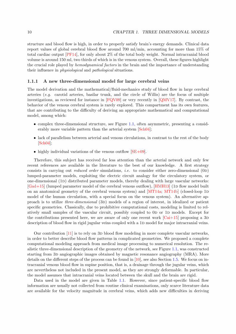
1.1.1 A new three-dimensional model for large cerebral veins
The model derivation and the mathematical/fluid-mechanics study of blood flow in large cerebralarteries (e.g. carotid arteries, basilar trunk, and the circle of Willis) are the focus of multipleinvestigations, as reviewed for instance in [FQV09] or very recently in [QMV17]. By contrast, thebehavior of the venous cerebral system is rarely explored. This compartment has its own features,that are contributing to the difficulty of deriving an appropriate mathematical and computationalmodel, among which:
• complex three-dimensional structure, see Figure 1.1, often asymmetric, presenting a consid-erably more variable pattern than the arterial system [Sch04];
• lack of parallelism between arterial and venous circulations, in contrast to the rest of the body[Sch04];
• highly individual variations of the venous outflow [SE+09].
Therefore, this subject has received far less attention than the arterial network and only fewrecent references are available in the literature to the best of our knowledge. A first strategyconsists in carrying out reduced order simulations, i.e. to consider either zero-dimensional (0d)lumped-parameter models, exploiting the electric circuit analogy for the circulatory system, orone-dimensional (1d) distributed parameter models, thereby dealing with large vascular networks:[Gad+15] (lumped parameter model of the cerebral venous outflow), [HMH13] (1d flow model builton an anatomical geometry of the cerebral venous system) and [MT14a; MT14b] (closed-loop 1dmodel of the human circulation, with a special focus on the venous system). An alternative ap-proach is to utilize three-dimensional (3d) models of a region of interest, in idealized or patientspecific geometries. Classically, due to prohibitive computational costs, modeling is limited to rel-atively small samples of the vascular circuit, possibly coupled to 0d or 1d models. Except forthe contributions presented here, we are aware of only one recent work [Cai+15] proposing a 3ddescription of blood flow in rigid jugular veins coupled with a 1d model for major intracranial veins.
Our contribution [11] is to rely on 3d blood flow modeling in more complete vascular networks,in order to better describe blood flow patterns in complicated geometries. We proposed a completecomputational modeling approach from medical image processing to numerical resolution. The re-alistic three-dimensional description of the geometry of the network, see Figure 1.1, was constructedstarting from 3d angiographic images obtained by magnetic resonance angiography (MRA). Moredetails on the different steps of the process can be found in [10], see also Section 1.5. We focus on in-tracranial venous blood flow in supine position, that is, a drainage through the jugular veins, whichare nevertheless not included in the present model, as they are strongly deformable. In particular,the model assumes that intracranial veins located between the skull and the brain are rigid.
Data used in the model are given in Table 1.1. However, since patient-specific blood flowinformation are usually not collected from routine clinical examinations, only scarce literature dataare available for the velocity magnitude in cerebral veins, which adds new difficulties in deriving

1.1. A MATHEMATICAL MODEL FOR THE VENOUS NETWORK 11
Figure 1.1: 1: internal jugular veins, 2: vein of Galen, 3: straight sinus, 4: confluence of sinuses,5: lateral sinus (transverse portion), 6: lateral sinus (sigmoid portion), 7: superior sagittal sinus, 8:internal cerebral vein, 9: basilar vein, 10: superior cerebral veins, 11: superior anastomotic veins.
Parameter Value Unit Source
Mass density ρ 1055 [ kgm3 ] [Thi08]
Dynamic viscosity µ 3.5 ·10−3 [Pa · s] [Thi08]
Cross-sectional velocity V ∗ (10− 11) · 10−2 [ms ] [HMH13](clinical studies, jugular vein) (8.5− 11.3) · 10−2 [ms ] [Ogo+11]
(30− 50) · 10−2 [ms ] [Sch04]Cross-sectional velocity V ∗ 15 · 10−2 [ms ] [Sch04]
(clinical studies, superior sagittal sinus) (15.2± 3) · 10−2 [ms ] [Gid+96]
Reynolds number (approx. values) [11]Internal jugular vein 90 − 232 −Superior sagittal sinus 90 − 144 −
Stokes number (approx. values) [11]Internal jugular vein 1.38 − 3.84 −Superior sagittal sinus 1.10 − 1.75 −
Strouhal number (approx. values) [11]Internal jugular vein 0.014 − 0.030 −Superior sagittal sinus 0.013 − 0.021 −
Table 1.1: Values of the mechanical and dimensionless parameters in the model.

12 CHAPTER 1. THREE DIMENSIONAL MODELS
an appropriate biomechanical model. We carefully performed a dimensional analysis of the modeland computed values for the Reynolds, Stokes, and Strouhal number, reported in Table 1.1. Theorder of magnitude of the Reynolds number shows the importance of the convective forces, whereasthe values of the Stokes and Strouhal numbers are important to assess the flow unsteadiness. Theanalysis shows that flow in the cerebral veins is governed by the Navier-Stokes equations for anincompressible viscous fluid, in a quasi-steady regime:
ρ∂u
∂t− 2∇ · (µD(u)) + ρ(u ·∇)u+∇p = 0, in Ω× I (1.1)
∇ · u = 0, in Ω× I (1.2)
endowed with appropriate initial and boundary conditions, where: u and p are the velocity andpressure of the fluid, D(u) = 1
2(∇u + ∇uT ) is the strain rate tensor, σ(u, p) = −pI + 2µD(u) isthe Cauchy stress tensor, ρ and µ are the density and dynamic viscosity of the fluid, respectively.
Concerning the initial status of the fluid velocity, it is well known that it has to be carefullyprescribed, since it should be divergence-free to be admissible. Unfortunately, in hemodynamiccomputations, this quantity is usually unknown, hence chosen equal to zero everywhere or, as abetter guess, as the solution of a stationary Stokes problem. We developed a solution to thisproblem in the preliminary work [18].
The issue of boundary conditions is of primary importance in simulating blood flow and a hugeliterature has been dedicated to this topic in the last years, as reviewed for instance in [FI14;QMV17]. In the context of the cerebral venous network, we proposed an extensive discussion onthis topic in [11], with the following partial conclusions:
• at the inflow, impose u = constant (small magnitude), since blood comes from the microcir-culation, modeled by a quasi-steady/steady Stokes flow;
• at the wall, impose u = 0, since intracranial veins are constrained between a nearly incom-pressible brain and the rigid skull;
• at the outflow, impose in a first approximation σ(u, p)n = 0 (the “do-nothing” classicalapproach).
Perspectives. A lot of subsequent questions are triggered by these choices, as for instance: howsmall (in terms of order of magnitude) should the inflow velocity be? How a rigid vessel model(acceptable for intracranial veins) could be coupled with a deformable vessel model (that is moreappropriate for jugular veins)? At the outflow: between using the “do-nothing” approach andcoupling with a reduced model involving a lot of parameters that are unavailable, which choice isbetter? We postpone the answers to some of these questions to Section 1.2 for a different theoreticalapproach [1] and to Section 1.3 for a sensitivity analysis study on the influence of different modelingassumptions [4]. We also discuss in Section 1.6 some questions left open and possible lines ofapproach.
1.1.2 Numerical results and discussion
The numerical strategy we implemented to compute approximate solutions to the previously derivedmodel involves a time-scheme based on the characteristics method [Pir82] and a spatial discretizationof finite element type, with P2/P1 inf-sup stable finite elements [BF12]. The numerical solvingapproach relies on the finite element library Freefem++ [Hec12]. More details about the parametersand numerical choices can be found in [11].

1.1. A MATHEMATICAL MODEL FOR THE VENOUS NETWORK 13
We display in Fig. 1.2 the simulated velocity field in the whole intracranial cerebral venousnetwork. We were able to identify a complicated three-dimensional flow behavior, with noticeablerecirculations in the confluence of the sinuses (bottom left panel). At the level of the superiorsagittal sinus, the flow is laminar (bottom right panel). An asymmetric behavior appears in arecirculation zone in the entrance segment of the right transverse sinus. This could be explained,at least partly, by the asymmetric architecture of the venous network.
Figure 1.2: Top: cerebral venous network, visualization of the flow patterns: instantaneous stream-lines, colored with velocity magnitude. Bottom: zoom on the velocity field in the confluence ofsinuses (left panel) and in the superior sagittal sinus (right panel).
An important question is the validation of these results, that we investigated as follows: thepredicted values of the velocity magnitude in the superior sagittal sinus range from 12.5 · 10−2m/sto 18 · 10−2m/s, consistently with clinical data, that is, 15 · 10−2m/s [Sch04] and 15.2± 3 · 10−2m/s[Gid+96], from a set of 14 control subjects using MR velocimetry. Flow rates calculated at inlets andoutlets are identical (∼ 8ml/s for an entry velocity uin = 50mm/s, corresponding to a physiologicalvalue [SE+09], hence guaranteeing mass conservation. Similar or slightly higher values, between10ml/s and 14ml/s for the outflow were reported in the literature [MT14a; MT14b]. Comparisonsbetween the model predictions of flow rate values at selected cross-sections with MRI measurementsreported in the literature are presented in Fig. 1.3.
Although these comparisons show satisfactory results, it should be noted that the clinicallyindicated patient measurements are not taken on the same geometry as the one used to perform oursimulations, but retrieved from reported data in the literature. Therefore, improving the validation

14 CHAPTER 1. THREE DIMENSIONAL MODELS
Figure 1.3: Comparison between MRI measurements of flow rates (ml/s) (average and standarddeviation) found in literature and our model in different locations of the intracranial venous network.SSS: Superior Sagittal Sinus, St. S: Straight Sinus, L. TS: Left Transverse Sinus, R. TS: RightTransverse Sinus.
process, using either in vitro or in vivo data is still a challenge, that will be further explored inSection 1.4.
1.2 A novel formulation of the Stokes system involving pressureboundary conditions
The issue of boundary conditions when modeling blood flow in the circulatory system is of majorimportance and matter of intense research. From the mathematical viewpoint, the well-posednessof the Navier-Stokes problem with different types of boundary conditions is a well-known difficultproblem. For essential boundary conditions, existence of a weak solution is proved for any Reynoldsnumber, but some issues about uniqueness are still open in the three-dimensional case: weak solu-tions exist on (0, T ) for all finite time T , but they are not necessarily unique, see e.g. [Ler33; Lio69;Tem01]. Existence and uniqueness theory is less complete for Neumann boundary conditions, due inparticular to the difficulty of establishing a priori estimates; we refer to [HRT96; QV03; BGM10] forresults in this sense. All these difficulties are inherited at the numerical level and a lot of researchefforts were devoted to devise appropriate numerical solutions, as recently reviewed in [QVV16,Section 3], see also [FI14].
When performing three-dimensional simulations for blood flow modeling, the domain is reducedto a region of interest and therefore, its boundary is composed of two parts: a physical boundary(corresponding to the vessel wall) and an artificial boundary (at the level where the vessel is trun-cated). On one hand, at the vessel wall, the no-slip Dirichlet condition is natural for a viscousfluid contained in a rigid domain, since the viscous effect constraints the fluid particles to adhereto the wall. On the other hand, at the artificial boundaries, different formulations with boundaryconditions involving components of the velocity field, stresses or pressure are of interest. Indeed,they should be able to take into account the rest of the closed circuit representing the circulatory
1.2. STOKES PROBLEM WITH PRESSURE BOUNDARY CONDITIONS 15
system. Moreover, in order to achieve physiological simulations, they should derive from clinicalmeasurements. However, in this case they might give rise to so-called defective boundary conditions:usually only average data are available to “feed” mathematical and computational models that re-quire pointwise data instead, see [FV12] or [Por+12] for different strategies in the context of bloodflow modeling.
In the particular case of the cerebral venous network, one of the main mechanisms that drivesthe flow and should be taken into account through appropriate boundary conditions is the pressuredrop. More generally, when modeling hydraulic network-like systems, for instance oil ducts, watersupply, microfluidic channels or biological flows, we are interested in the case when the velocityfield is imposed on one part of the boundary and pressure values are prescribed, together with thecondition of no tangential flow, on the remaining part. We present in this section a new method weproposed in [1] to take into account these non-standard boundary conditions, both at the continuousand the discrete levels, in a finite-element framework.
1.2.1 General framework and the Lagrange multiplier formulation
We consider the steady state of a viscous incompressible fluid at low Reynolds number, describedby the velocity and pressure fields u and p that satisfy the following Stokes equations:
−2µ∇ · (D(u)) +∇p = ρf , in Ω, (1.3)
∇ · u = 0, in Ω, (1.4)
u = 0, on Γ1, (1.5)
u× n = 0, on Γ2, and (1.6)
p = p0, on Γ2, (1.7)
where
∂Ω = Γ1 ∪ Γ2, with Γ1 ∩ Γ2 = ∅ and such that each connected component of Γ2 is flat,
represents a partition without overlap of the boundary of Ω and n indicates the outward normal to∂Ω. The notations are similar to Section 1.1, the function f is a given external force, the functionp0 a given pressure, and d = 2, 3 is such that Ω ⊂ Rd.
A variational formulation taking into account this type of boundary conditions was first intro-duced in the seminal works [Pir86; Beg+87; CMP94]. A lot of subsequent literature was devotedto this topic, see [1] for an in depth discussion about the method in the context of the existingliterature.
Remark 1.2.1. Previous works [Pir86; Beg+87; CMP94; Con+95; BCRY15] classically take intoaccount non standard boundary conditions of type (1.5–1.7) by expressing the conservation of themomentum in terms of the Laplacian of the velocity and then using as a key ingredient the rotationalformulation for the equation, based on:
−Δu = ∇× (∇× u)−∇(∇ · u).Although at a continuous level the two formulations are equivalent, since
∇ · u = 0 ⇒ ∇ · (∇u+∇uT ) = Δu,
from a modeling standpoint it may be useful to work with the symmetric tensor. For instance, influid-structure problems, formulation (1.3–1.7) gives directly the natural boundary condition for thestructure problem in terms of the force exerted by the fluid on its boundary. We thus focus hereafteron the formulation in terms of the divergence of the symmetric gradient (1.3).

16 CHAPTER 1. THREE DIMENSIONAL MODELS
We showed in [1] that the problem can be written as follows:
Problem 1.2.2. Find u ∈ V , p ∈ M , λ ∈ Λ such that for all v ∈ V , q ∈ M , η ∈ Λ
2µ
�
ΩD(u) : D(v) dx−
�
Ωp∇ · v dx− c(v,λ) = ρ
�
Ωf · v dx−
�
Γ2
p0n · v ds (1.8)
�
Ωq∇ · u dx = 0 (1.9)
c(u,η) = 0. (1.10)
The functional spaces are defined as V = {v ∈ [H1(Ω)]d : v = 0 on Γ1}, M = L2(Ω), andΛ = [H−1/2(Γ2)]
d−1. The bilinear form c : V ×Λ → R is given by
c(u,λ) =
�
Γ2
u · i(λ) dx
where i : [H−1/2(Γ2)]d−1 → T is an isomorphism and
T =�ζ ∈ [H−1/2(Γ2)]
d : ζ · n = 0�.
Details on how the bilinear form c is built in practice in two and three dimensions, by makingexplicit the isomorphism between T and Λ can be found in [1]. We have the following theorem:
Theorem 1.2.3. Problem 1.2.2 admits a unique solution (u, p,λ) which verifies
�u�1,Ω + �p�0,Ω + �λ�−1/2,Γ2� �f�V � + inf
v∈V
�Γ2
p0n · v ds
�v�1,Ω� �f�0,Ω + �p0�0,Γ2 .
Moreover, if u ∈ [C2(Ω)]d, p ∈ C1(Ω), then (u, p) is the solution of (1.3–1.7) and λ verifies
i(λ) = τ (u, p),
where τ (u, p) is the tangential component of the normal traction σ(u, p)n.
The proof is based on the interpretation of Problem 1.2.2 as a double saddle-point problem and onestablishing the two corresponding inf-sup conditions.
Remark 1.2.4. It is clear that the Lagrange multiplier formulation described in Problem 1.2.2 isnot straightforward to use in practice, since it introduces supplementary unknowns that increasethe complexity of the numerical solution. Nevertheless, this novel formulation allows for pressureboundary conditions with L2 regularity on the boundary. This result was believed possible but wasnot covered by the analysis in [BCRY15], as discussed by the authors in Sec. 6. Moreover, while theprevious treatment of the Laplacian expressed by a rotational formulation required more regularity onthe pressure and a velocity field with smooth curl and div components [CMP94; Gir90; BCRY15],Theorem 1.2.3 proves the existence of a solution to the Stokes problem (1.3–1.7) in the same H1×L2
functional spaces as for standard boundary conditions.
Discretization of Problem 1.2.2. We introduce a compatible tessellation Th of the domain Ω intetrahedral or hexahedral elements [1]. On Th, we introduce piecewise polynomial spaces Vh ⊆ V ,Qh ⊂ M , respectively approximating velocity and pressure, and we assume that such spaces satisfythe standard inf-sup condition
infph∈Q0
h
supuh∈Vh∩[H1
0 (Ω)]3
�Ω ph∇ · uh dx
�uh�1,Ω�ph�0,Ω� 1. (1.11)

1.2. STOKES PROBLEM WITH PRESSURE BOUNDARY CONDITIONS 17
(where Q0h =
�qh ∈ Qh :
�Ω qh = 0
�), so that they provide a stable discretization of the Stokes
problem with standard Dirichlet boundary conditions. We now observe that Vh|Γ2 = [Wh]3 where
Wh is itself a finite element space on the two-dimensional mesh T Γ2h induced on Γ2 by the three-
dimensional tessellation Th. Remark (see the definition of the space V ) that the functions in Wh
satisfy homogeneous boundary conditions on ∂Γ2. We then let Λh = [Wh]2. We consider the
following discrete problem:
Problem 1.2.5. Find uh ∈ Vh, ph ∈ Qh, λh ∈ Λh such that for all vh ∈ Vh, qh ∈ Qh, ηh ∈ Λh
2µ
�
ΩD(uh) : D(vh) dx−
�
Ωph∇ · vh dx− c(vh,λh) = ρ
�
Ωf · vh dx−
�
Γ2
p0n · vh ds,(1.12)
�
Ωqh∇ · uh dx = 0, (1.13)
c(uh,ηh) = 0. (1.14)
The following theorem then holds:
Theorem 1.2.6. There exists h0 such that, if h ≤ h0, Problem 1.2.5 admits a unique solution(uh, ph,λh) which verifies
�uh�1,Ω + �ph�0,Ω + �λh�−1/2,Γ2� �f�0,Ω + �p0�0,Γ2 .
Moreover the following error estimate holds:
�u− uh�1,Ω + �p− ph�0,Ω � infvh∈V 0
h
�u− vh�1,Ω + infqh∈Qh
�q − qh�0,Ω,
whereV 0h = {uh ∈ Vh : c(uh,λh) = 0, ∀λh ∈ Λh} .
Once again, as in the continuous case, the proof of Theorem 1.2.6 reduces to prove two inf-supconditions.A direct consequence of this result is that for the classical case of Taylor-Hood inf-sup stable finiteelement spaces [BF12]:
Vh = {u ∈ [C0(Ω)]3 : ∀K ∈ Th u|K ∈ [Pk(K)]3}, (1.15)
Qh = {p ∈ C0(Ω) : ∀K ∈ Th p|K ∈ Pk−1(K)}. (1.16)
and for u ∈ [Hk+1(Ω)]3 and p ∈ Hk(Ω) we have
�u− uh�1,Ω + �p− ph�0,Ω � hk(�u�k+1,Ω + �p�k,Ω). (1.17)
We thus expect optimal convergence rates provided the solution has sufficient regularity.
Remark 1.2.7. We emphasize that there is no reason why the multiplier i(λ) = τ (u, p) shouldvanish at the boundary of Γ2. Therefore, the proposed discretization cannot, in general, yield anoptimal approximation of the Lagrange multiplier. Nevertheless, since V0
h ⊂ V0, the approximationproperties for the Lagrange multiplier do not enter the error estimate in Theorem 1.2.6, and we getan optimal error estimate for both velocity and pressure.
Remark 1.2.8. Throughout the study, we assumed that Γ2 was a flat surface (or, more precisely,we assumed that n was constant on the connected components of Γ2). Let us consider two cases inwhich this assumption is not satisfied.

18 CHAPTER 1. THREE DIMENSIONAL MODELS
If a connected component of Γ2 is the union of two (or more) flat subregions sharing a vertex(in 2d) or an edge (in 3d), we observe that, at the continuous level, if n1 and n2 are constant unitnormals to the two subregions with direction chosen in such a way that on the common vertex or edgewe have u = |u|n1 = |u|n2, if n1 �= n2 then u = 0, so that the solution vanishes at the interfacebetween the two subregions. At the discrete level one needs then to strongly force the velocity tovanish on such interface. Once this is done, the analysis presented above remains valid.
If, on the other hand, Γ2 is a curved surface, the situation is more complex. At the continuouslevel, we show that the natural boundary condition implicit in equation (1.8) is not (1.7), but rather
p+ 2µ|u|κ = p0, on Γ2, (1.18)
where κ is the mean curvature of Γ2. Nevertheless, Problem 1.2.2 is still well posed, and Theorem1.2.3 still holds, provided equation (1.7) is replaced by equation (1.18). Things are more complexwhen it comes to discretization Problem 1.2.2, since part of the arguments used in the proof of The-orem 1.2.6 do not hold for curved boundaries. In addition, if the normal to the discrete boundaryhas jumps (which would automatically happen when approximating a curved boundary with a finiteelement mesh), similar arguments show that the whole method would then be non conforming. Re-mark that we might also need to resort to a non conforming discretization if we drop the requirementthat the tessellation Th is compatible with the splitting of ∂Ω into Γ1 ∪ Γ2.
1.2.2 Numerical results and applications
The computational framework is developed in Feel++, Finite Element Embedded Library in C++[Fee], see for more details Section 1.4. Regarding the specific implementation of the proposedmethodology, we would like to point out some non-standard aspects, namely the treatment of theterms associated to the Lagrange multipliers. Feel++ provides a mechanism to extract submeshesof faces and keep a relation between the extracted mesh and the parent mesh. The relation is nec-essary to ensure an efficient treatment of the coupling terms between the velocity and the Lagrangemultipliers. The geometrical data, i.e the normals, are automatically deduced from the parentmesh.
We evaluated the performances of the method proposed in Section 1.2.1 when solving two typesof problems: (i) study of the convergence properties of the method for different choices of finiteelements, (results not reported here, available in [1]); (ii) a 3d computational model of the cerebralvenous blood flow similar to the one described in Section 1.1, but incorporating pressure boundaryconditions (in a first approximation for low Reynolds numbers).
Figure 1.4 displays the pressure field (top left panel) and instantaneous streamlines, colored withvelocity magnitude (top right panel), illustrating the pressure drop effect and a complicated three-dimensional flow behavior. The overall dynamics shares common features with the one we foundin Section 1.1, but a direct comparison would not be meaningful at this stage, since here only theStokes equations are solved. The order of magnitude of the maximum velocity is slightly higher thanvalues retrieved in the clinical literature, see for instance [Sch04], therefore more precise values needto be included in further work. However, the development of a computational model able to capture,to this level of accuracy, different features of the flow can be seen as a very promising approachfor analyzing, by means of numerical simulations, the dynamics of flow patterns in morphologicallycomplex vascular districts.
Remark 1.2.9. A zoom on some inlet, respectively outlet sections is presented in Figure 1.5,demonstrating that the flow is normal to both inflow and outflow surfaces. We highlight the interestof imposing the pressure value and the zero tangential component of the velocity in this context: thecurrent formulation allows to retrieve a Poiseuille-like behavior that is physically meaningful when

1.2. STOKES PROBLEM WITH PRESSURE BOUNDARY CONDITIONS 19
Figure 1.4: Cerebral venous hemodynamics obtained by imposing a pressure drop between the inletand outlet sections, pressure field (left panel) and streamlines (right panel).
dealing with artificial boundary conditions, while keeping the viscous stress tensor in the expressionof the Stokes problem, useful from a modeling standpoint. In contrast, as noted in [LG81; HRT96],using the symmetric gradient 1
2(∇u+∇uT ) and prescribing the normal stress at the outlet lead toa non-physical representation of the flow: the velocity vectors “spread” like at the end of a pipe,instead of mimicking the fact that the network continues after this artificial section. Alternatively,the non symmetric tensor ∇u can be used to recover the Poiseuille exact solution in a cylinder, butthe physical meaning of such a boundary condition is not clear.
Figure 1.5: Zoom on velocity vectors at some inlet sections (left panel), respectively outlet sections(right panel).
Perspectives. The current methodology should be further developed, in particular by (i) devisingan adapted discretization strategy for the case of a curved boundary, in order to overcome thedifficulties briefly discussed in Section 1.2.1; (ii) improving linear solvers scalability by means of well-suited block-preconditioning strategies; (iii) extending the present analysis to the incompressibleNavier-Stokes equations [BCRY15] and to Generalized non-Newtonian models in the context ofblood flow modeling described in [FQV09, Chap. 6]. Furthermore, an exploration of the close

20 CHAPTER 1. THREE DIMENSIONAL MODELS
Figure 1.6: Representation of the relative importance of various factors in models of the differenthemodynamic scales: ++ indicates primary importance; −− indicates secondary or negligible im-portance; ?? indicates potential or unclear importance (taken from Creative Commons and [Ste12]).
connection between Lagrange multipliers technique and a classical method by Nitsche as suggestedin [Ste95; Ver11] provides a promising perspective of the present work.
1.3 Influence of different modeling assumptions
The complexity of the human circulatory tree and the underlying bio-mechanical phenomena callfor various simplifications in view of designing and implementing mathematical and computationalmodels. The relative importance of these assumptions is difficult to establish and quantify. There-fore a lot of open questions still remain, see Figure 1.6 and extended discussion in [Ste12]. Inaddition, as already emphasized in Section 1.1, the venous network is far less known and studiedin comparison to the arterial one. For arteries, recent contributions assessed the impact of viscos-ity models and flow conditions in aneurysms [EVSM13] or of the assumption of laminar flow incomputational hemodynamics, taking cerebral aneurysms as an illustrative example [EM15].
In line with these studies, the goal of [4], summarized in this section, is to assess in a soundmathematical and computational framework the effect of different modeling assumptions on cerebralvenous blood flow dynamics at a macroscopic scale.
1.3.1 Sensitivity analysis framework
Formulation of the problem. We consider, as a starting point, the Navier-Stokes system (1.1)-(1.2) for large and medium-sized cerebral veins introduced in Section 1.1.1 with two extensions:
• a Generalized Newtonian constitutive law for blood flow, in addition to the Newtonian modelfrom Section 1.1.1;
• the coupling with a simplified 0d model at the outflow, as an alternative to the traction-freeboundary condition used in Section 1.1.1.
More precisely, the viscosity is considered either constant, when adopting a Newtonian consti-tutive model, or as a function of the shear rate:
γ =
�2tr
�D (u)2
�, (1.19)

1.3. INFLUENCE OF DIFFERENT MODELING ASSUMPTIONS 21
when using a Generalized Newtonian model. In [4], we focused on the comparison between theNewtonian model, and the Carreau and Carreau-Yasuda Generalized Newtonian constitutive modelsfor blood [FQV09, Chap. 6], that return the viscosity as a function of the shear rate by the followingequation:
µ(γ)− µ∞µ0 − µ∞
= (1 + (λγ)a)n−12 , (1.20)
where λ is a time constant, a and n are dimensionless parameters used to differentiate between thetwo models, and µ0 and µ∞ are the viscosities at zero and infinite shear rate, respectively.
Regarding the boundary conditions: at the inflow, we impose a constant profile of small magni-tude and at the vessel wall u = 0, since we considered it to be rigid. A more general setting is usedfor the outflow: boundary conditions are prescribed either by using a traction-free condition as inSection 1.1.1:
σ(u, p)n = 0 on Γout, (1.21)
or by introducing the coupling with a three-element Windkessel model [FQV09, Chap. 10], in orderto take into account the downstream vasculature. In the latter case, the condition reads:
σ(u, p)n = −Pln on Γout, (1.22)
where Pl (the proximal pressure) is obtained by solving
Cd,ldπldt
+πlRd,l
= Ql
Pl = Rp,lQl + πl,
(1.23)
for a given value of the flux on the outlet Ql =�Γout
u · n dx.
Discretization. We use a fully implicit time discretization using BDFη scheme, including forthe non-Newtonian models, with non-linear solving handled by a Newton method. The time-discretization of Equations (1.1)–(1.2) in the Newtonian case is written as follows:
ρ
��ηk=0 αku
n+1−k
Δt+ un+1 ·∇un+1
�−∇ · (−pn+1I+ 2µD(un+1)) = 0,
∇ · (un+1) = 0,
(1.24)
where (αk)k=0,η are the BDFη coefficients for the time derivative of u and the subscript η refersto the order of the scheme. We adopted the BDF1 (η = 1) and BDF2 (η = 2) schemes forthe time approximation. The spatial discretization is handled via a inf-sup stable finite element(Taylor-Hood) P2/P1 [BF12]. Our numerical strategy is in line with [VSS14] as we performed highresolution simulations and not normal resolution simulations: both the spatial and the temporaldiscretization methods are second-order schemes and a small time step (Δt = 10−3s) was chosen,in order to adequately resolve the complex flow features.
Sensitivity analysis framework The idea stems from [Evj11], where the author defines twometrics, one for the velocity and one for the wall shear stress, in order to improve the visualcomparison between snapshots of solutions by assessing the differences between two solutions in amore quantitative manner. Both metrics require to define a computed reference solution and thenthe computation of the time evolution of the average on the entire mesh of some specific quantities,which reflect point-wise differences between velocities and the wall shear stresses, respectively. This

22 CHAPTER 1. THREE DIMENSIONAL MODELS
approach has in addition the advantage of assessing the time evolution of these differences, whereascomparisons of snapshots are only showing spatial differences at some selected instants.
The first metric measures the difference between the computed solution (uC) and the computedreference solution (uR). To this end, following [Evj11], we define the spatial metric for each timestep
SuR(uC) = 1− βe−a − γe−m, (1.25)
where
a =1
πcos−1
�uR · uC
�uC��uC�
�, 0 ≤ a ≤ 1, (1.26)
m =�uR − uC�
�uR�, 0 ≤ m and β = γ =
1
2. (1.27)
The value a corresponds to the scaled angle between the two vectors and the value m to relativedifference in their order of magnitude. The spatial average is then computed by:
Du =1
V
�
ΩSuR(uC) dx, where V =
�
Ω1 dx. (1.28)
The second metric measures the difference between the computed reference solution of the wallshear stress τR and another numerical solution of the wall shear stress τC . Again, following [Evj11],we define the spatial metric for each time step as
TτR(τC) = 1− e−t, t =
����τR − τC
τR
���� (1.29)
and its spatial average
Dτ =1
S
�
∂ΩTτR(τC) dx, where S =
�
∂Ω1 dx. (1.30)
Remark 1.3.1. In practice, very intensive parallel computation are required to obtain the metrics(the studies used from 64 to 512 cores and ranged from 1 million to about 10 millions degrees offreedom). In our case, they were almost as expensive as some of the actual numerical simulationsand therefore an efficient high performance computational framework was needed, see for moredetails Section 1.4.
1.3.2 Numerical results and discussion
The sensitivity analysis study was carried out in the open-source library Feel++ [Fee]. First, wecarefully assessed the impact of the numerical strategy in use, see [4] and second, we investigatedthe impact of several modeling assumptions in a controlled numerical environment.
We illustrate here the outcomes of our study in the specific case of the influence of the inletvelocity magnitude imposed at each inflow. Detailed results for the other modeling assumptions(outflow treatment and viscosity models) are reported in [4]. The simulations were performed forseveral models (Newtonian 3d, non-Newtonian 3d and Newtonian 3d-0d). In each case, we takethe reference solution with an inlet velocity magnitude equal to 10−3 m
s . Then, we compute theinfluence of each model by taking vin = 20−3 m
s and vin = 30−3 ms , respectively.
The results are displayed in Figure 1.7, where a grid refinement study is reported, and inFigure 1.8, where different models are compared. The mesh convergence tests were performedon three meshes M0, M1 and M2 described in Table 1.2 and applied to the computed reference

1.3. INFLUENCE OF DIFFERENT MODELING ASSUMPTIONS 23
solution uR. Both metrics are persistently higher in comparison with the case of the outflow orrheological model, with a significant non-linear increase in the case of the wall shear stress metric.This should be compared to a Poiseuille approximation, frequently used in blood flow modeling,that predicts a linear increase of the wall shear stress when the velocity increases linearly. In thepresent case, where blood flow dynamics is complex and the geometry is also very complicated, thisapproximation is no more valid. It can also be noted that Newtonian 3d and Newtonian 3d-0dmodels present the same sensitivity for both velocity and wall shear stress metric; the same behaviorcan be found when comparing the two non-Newtonian models. Moreover, we can see in these figuresthat the non-Newtonian models have less influence compared to the Newtonian models on the samequantities. This effect is more significant in wall shear stress metric, but it is also visible in thevelocity metric.
h Nelt Ndof
m0 0.03 322 013 1 640 236m1 0.02 985 484 4 717 123m2 0.015 2 008 757 9 171 904
Table 1.2: Mesh convergence tests; h: characteristic element size, Nelt: number of tetrahedra, Ndof :number of degrees of freedom.
0.0 0.2 0.4 0.6 0.8 1.0time [s]
0.0
0.2
0.4
0.6
0.8
1.0
velo
city
met
ric
M0M0
M1M1
M2M2
0.0 0.2 0.4 0.6 0.8 1.0time [s]
0.0
0.2
0.4
0.6
0.8
1.0
wss
met
ric
M0M0
M1M1
M2M2
Figure 1.7: Effects of inlet velocity magnitude vin. The reference solution for each level mesh iscomputed using vin = 10−3 m
s . Continuous lines correspond to vin = 20−3 ms and dashed lines to
vin = 30−3 ms .
Conclusions and outlook. The results of the present study showed that for cerebral veins bloodflow modeling, the impact of setting the inlet boundary condition on the forces created by blood flow,is likely greater than for other modeling assumptions. Therefore, they highlighted the importance ofderiving values for these conditions from clinically measured data at some probe locations, in orderto enhance the accuracy of the computed hemodynamical quantities of interest. These findingsare significant in the perspective of the integration of the computational modeling step in a fullpipeline, where the interaction at the stage of acquisition of data and also in the validation processtakes place, see Section 1.5. From the mathematical and numerical standpoint, only a deterministicapproach was used in the present sensitivity analysis study, but next steps should also include

24 CHAPTER 1. THREE DIMENSIONAL MODELS
0.0 0.2 0.4 0.6 0.8 1.0time [s]
0.30
0.32
0.34
0.36
0.38
0.40
0.42
0.44
0.46
velo
city
met
ric
Newtonian 3DFREENewtonian 3DFREENewtonian 3DW1Newtonian 3DW1
Carreau 3DFREECarreau 3DFREECarreau-Yasuda 3DFREECarreau-Yasuda 3DFREE
0.0 0.2 0.4 0.6 0.8 1.0time [s]
0.4
0.5
0.6
0.7
0.8
0.9
wss
met
ric
Newtonian 3DFREENewtonian 3DFREENewtonian 3DW1Newtonian 3DW1
Carreau 3DFREECarreau 3DFREECarreau-Yasuda 3DFREECarreau-Yasuda 3DFREE
Figure 1.8: Effects of inlet velocity magnitude vin. The reference solution for each model is computedby using vin = 10−3 m
s . Continuous lines correspond to vin = 20−3 ms and dashed lines to vin =
30−3 ms .
quantification of statistical variability in these data. In this direction, we proposed a first attemptfor a simplified 0d model in [21], see Section 2.2.1.
1.4 Large-scale blood flow simulations and validation
In this section we present our continuous efforts to develop a powerful and flexible computationalframework [6] for numerically solving problems arising in hemodynamics, such as [4; 1]. We alsodiscuss our contribution towards improving the reliability and reproducibility of computationalstudies by performing a thorough validation of the fluid solver against experimental data [5].
1.4.1 Computational framework
The core of the framework is the Finite Element Embedded Library in C++ Feel++, that allowsto use a very wide range of Galerkin methods and advanced numerical techniques such as domaindecomposition (including mortar and three fields methods), fictitious domain or certified reducedbasis. The ingredients include a very expressive embedded language, seamless interpolation, meshadaption and seamless parallelization. Feel++ provides a mathematical kernel for solving partialdifferential equation using arbitrary order Galerkin methods in 1d, 2d, 3d and on manifolds usingsimplices and hypercubes meshes [Pru+12]:
• a polynomial library allowing for a wide range polynomial expansions including Hdiv and Hcurl
elements;
• a light interface to Boost.UBlas, Eigen3 and PETSc [Bal+16]/SLEPc as well as a scalablein-house solution strategy;
• a language for Galerkin methods starting with fundamental concepts such as function spaces,forms, operators, functionals and integrals;
• a framework that allows user codes to scale seamlessly from single core computation to thou-sands of cores and enables hybrid computing.

1.4. HPC AND VALIDATION 25
First steps towards large-scale three-dimensional blood flow simulations in realistic geometrieswere achieved in [6], where we investigated several issues: (i) handling various boundary conditionssettings allowing for a flexible framework with respect to the type of input data (velocity, pressure,flow rate . . .); (ii) handling of the discretization errors not only with respect to the physical fields(velocity and pressure) but also with respect to the geometry; (iii) dealing with the associated largecomputational cost, requiring high performance computing, through strong and weak scalabilitystudies.
On the basis of the problems studied in [4; 1], we added new capabilities in the algebraic solvingframework. To give an insight about the importance of the preconditioning strategy when solvingcomplex flow problems, we gather in Table 1.3 results allowing for a direct comparison betweenthree possible choices in term of preconditioners when computing the solution of a pressure-drivenStokes flow in the cerebral venous network [1]. Strategy PGASM couples monolithically a Kryloviterative solver with an additive Schwarz preconditioner, whereas Strategies PBlock
1 and PBlock2
couple a Krylov iterative solver with a block preconditioning strategy, following [ESW14]. To applythis framework, we remark that we deal with a double saddle point problem: we gather eitherthe velocity-pressure unknowns or the velocity-Lagrange multiplier unknowns to setup a two levelpreconditioner.
Strategy PGASM Strategy PBlock1 Strategy PBlock
2
m0 163[420] 20[174] 67[86]m1 366[393] 45[267] 161[123]m2 1080[429] 84[369] 271[143]m3 4616[522] 293[660] 707[196]m4 x 898[791] 1960[175]
Table 1.3: Time comparison for three preconditioning strategies (in seconds). In brackets, thenumber of iteration used by solver.
Simulations were performed with 96 processors and the time is measured in seconds. Thecomparison clearly shows the limits of Strategy PGASM and the gain in terms of computationaltime when choosing Strategy PBlock
1 and Strategy PBlock2 . Note that in the Strategy PBlock
1 , thenumber of iterations grows strongly with respect to the problem size. Further refinements regardingthe different choices are required and will be subject of future research.
1.4.2 The FDA benchmark nozzle model
A challenging benchmark was proposed by the US Food and Drug Administration (FDA) in[Har+11] in order to assess the stability, accuracy and robustness of computational methods indifferent physiological regimes. The findings of 28 blinded investigations were reported in [Ste+13]and, as critically analyzed in [Sot12], practically all CFD solvers failed to predict results that agreedin a satisfactory manner with the experimental data. Several subsequent papers tackled this ques-tion, by employing different numerical approaches, see [5] for a more detailed discussion.
The benchmark provides a comprehensive dataset of experimental measures using a well-definedgeometry corresponding to an idealized medical device (see Figure 1.9 for a schematic sketch of thedomain and [Har+11, Sec. 2.1] for more details). Five sets of data spanning laminar, transitionaland turbulent regimes are made available on-line and the device was designed to feature accelerating,decelerating and recirculating flow (all of which occur in real medical devices). We investigated in

26 CHAPTER 1. THREE DIMENSIONAL MODELS
Figure 1.9: FDA nozzle sketch and specifications (from [Har+11]).
[5] three flow regimes, corresponding to a Reynold number at the throat level ReThroat = 500, 2000and 3500, by using a direct numerical simulation method for the Navier-Stokes equations. A detailedreport of the numerical method and parameters used for each test can be found in [5]. In particularwe implemented and compared low order as well as high order approximations including for thegeometry and we discussed some issues not previously reported in the literature.
The comparison with experimental data is made in terms of (i) wall pressure difference (nor-malized to the mean throat velocity) versus axial distance; and (ii) axial component of the velocity(normalized to the mean inlet velocity) along the centerline:
Δpnorm =pz − pz=0
12ρfu
2t
and unormz =uzui
, where ut =4Q
πD2t
, ui =4Q
πD2i
, (1.31)
and Q is the volumetric flow rate. Furthermore, two validation metrics reported in [Ste+13] werecomputed: a conservation of mass error metric EQ (on a percentage basis) and a general validationmetric Ez comparing average experimental velocity data with computed axial velocities.
We only provide here illustrative numerical results corresponding to ReThroat = 500; for allthe other cases, see [5]. Four mesh refinement levels, denoted M0–M3, from the coarsest to thefinest level, were constructed. Several polynomial order approximations were used and the notationPN+1PNGkgeo specifies the discretization spaces for the velocity, pressure, and geometry, respec-tively. Figure 1.10 shows the results for the normalized axial velocity and the normalized pressuredifference along the z axis, respectively. In each case, we can see very satisfactory agreement withthe experimental data.
We illustrate in Figure 1.11 the computation of metrics Ez and EQ for several mesh refinementsat ReThroat = 500. The metric Ez takes small values in each numerical experiment, identifying agood agreement between computed and experimental data, and displays only small variations withrespect to mesh refinement. On the other hand, the metric EQ is more sensitive to this factor:error does not exceed the ∼ 2%, except for the coarse mesh M0 where, in two locations, the errorincreases up to ∼ 10%. Interestingly, we note that the P3P2G1 approximation does not improvethe results for the coarse mesh, but that a satisfactory error below 2% is retrieved when using aP2P1G2 approximation.
Additional tests to complement the study of the impact of high order approximation are ongoingand an extended version of [5] is planned to be submitted for publication.

1.4. HPC AND VALIDATION 27
Figure 1.10: ReThroat = 500, experimental data vs. numerical results: normalized axial velocity(left); normalized pressure difference along z (right).
Figure 1.11: ReThroat = 500: validation metrics Ez (left) and EQ (right).

28 CHAPTER 1. THREE DIMENSIONAL MODELS
1.5 An open-source framework to generate virtual MRA imagesfrom real MRA images
In the previous sections, we presented several contributions to develop a sound mathematicaland computational framework for hemodynamic simulations, with an emphasis on applicationsto the cerebral venous network. This methodology was integrated in the interdisciplinary programVIVABRAIN Virtual angiography simulation from 3D and 3D+t brain vascular models [Viv], thataims at starting from real MR angiographic data to finally lead to the generation of virtual MRangiographic data. We summarize hereafter the main steps and challenges of these developments.
As explained in Section 1.1, the realistic data we used as a starting point were acquired using dif-ferent Magnetic Resonance Angiography (MRA) sequences. MRA is an image acquisition techniqueparticularly used, for instance, in the case of detection and diagnosis of vascular alterations (e.g.,stenoses, aneurysms, thromboses), and patient follow-up after treatment (e.g., by stents, coils).MRA is also an effective tool for clinical research devoted to the understanding of human macroand mesovascular physiology, since it provides non-invasive/non-ionizing modalities (e.g., PhaseContrast (PC) or Time-of-Flight (TOF) MRA), available in 2d, 3d, and even 3d+time.
Due to the nature of structures visualized in MRA, namely thin, elongated, curvy vessels, thedevelopment of specific image analysis tools has been an active research area during the last decades[Les+09]. However, contrary to other morphological structures (e.g., brain tissues and structures,with BrainWeb [Coc+97]), there is no common framework to facilitate the development and vali-dation of related image analysis methods. In particular, despite a few attempts (such as [Sch+09]),that rely on datasets equipped with manual ground truth, there is no vascular analogue of Brain-Web, i.e., a framework for generating efficiently virtual MRA images naturally equipped with aground-truth and/or associated to a real MRA. Stemming on this fact, we have been working, inthe context of the VIVABRAIN project with the final goal to tackle this issue, knowing that thecase of virtual MRA was not intensively considered, in particular via the efficient coupling of CFDand MRI simulation.
The framework relies on a pipeline composed of five main steps, going from real MRA to virtualMRA, see Figure 1.12:
(i) MRA acquisition;
(ii) segmentation of vascular volumes from such data and design of a vascular model, in particularby explicitly modeling anatomical and physiological features;
(iii) construction of computational meshes of the vascular structures;
(iv) simulation of the flowing blood in the designed vascular model, leading to velocity and pressurefields;
(v) generation of virtual MRA images based on the previously computed information.
Our contributions are inserted in step (iv), with natural ramifications in the pre- and post- pro-cessing steps, namely building the computational meshes before the simulations and treating theresults afterwards. Besides the inherent challenges related to the mathematical and computationalapproach, additional difficulties come into play. In particular, the complexity of the data to handleat the interface between the steps and their representation is a crucial point: for instance, fluidsimulations are performed in an Eulerian framework, whereas MRA simulation in performed by

1.6. CONCLUSIONS AND OUTLOOK 29
Figure 1.12: VIVABRAIN pipeline.
numerically solving the Bloch equations with a Lagrangian-based approach.
These research efforts were first presented in [10], where the workflow from medical images tonumerical simulations was discussed. A significant step forward was achieved by junior researchersof the VIVABRAIN project in [Anc+16]: a validation process of the entire VIVABRAIN pipelinewas performed on a physical phantom (a double bifurcation fluid circuit), on which morphologicaland flow data were acquired within the project. The most up-to-date full methodological frameworkis described in [13]. A software pipeline is associated to this framework [Ang] and open-data is acomplementary purpose of the software framework, itself developed in an open-source way. It willhopefully constitutes a versatile tool for progressing in the understanding of vascular networks, espe-cially in the brain, and the associated imaging technologies. Furthermore, it provides the foundationof a reliable and efficient computational framework allowing for a computer-aided interpretation ofclinical data, as available in the Eye2brain project that will be discussed in the next sections.
1.6 Conclusions and outlook
Our contribution with respect to existing works on three-dimensional models for blood flow in re-alistic geometries considered the importance of boundary conditions, with a focus on the cerebralvenous network. We developed the first three-dimensional sound mathematical and computationalmodel for the venous part of the cerebral vasculature, that complements previous works on thearterial side and on reduced models for the same compartment. The framework incorporates a newLagrange multiplier-based numerical method to take into account boundary conditions involvingpressure, that we throughly analyzed in the case of the Stokes problem. We also made first stepsto take into account uncertainties in different modeling assumptions through a sensitivity analysisapproach, in a high performance computing framework that was validated on significant bench-marks. Finally, all these contributions were integrated in a general software pipeline for generatingefficiently virtual MRA images naturally associated to a real MRA.

30 CHAPTER 1. THREE DIMENSIONAL MODELS
In addition to the specific extensions discussed in each section, we present hereafter some overallperspectives on the topic. Eventually, this mathematical and computational modeling frameworkcould contribute to elucidate the numerous open questions connecting brain venous hemodynamicsand neurological diseases, as recently reviewed in [Tor16].
Multiscale approach. By means of the new algorithm we developed in [3] (see Section 2.3), weaim at building amultiscale model that couples the 3D intracranial description of the venous network[11] with the reduced 0d model of the extra-cranial drainage pathways proposed in [Gad+15]. Wemade a first step by coupling the three-dimensional domain with a very simple Windkessel modelin Section 1.3, that already gave promising results. However, in our current model, only two maindrainage veins in the supine position are included (corresponding to the jugular veins), due to thelimitations of the image acquisition process. The advantage of this new multiscale model is thatit would allow to add a more sophisticated description of the collateral pathways that were veryrecently shown to play an important role as an alternative route for venous outflow according to thesubject position, that is, standing or sitting [Gis+04; SE+09]. From the mathematical viewpoint,that would require extending our algorithm to the Navier-Stokes system, as explained in Section2.3, and improving linear solvers efficacy by means of well-suited block-preconditioning strategies inthe spirit of [ESW14]. More generally, incorporating the possibility to describe by a reduced modela part of the entire vascular tree would be meaningful to tackle the issue of parameter identification,in line with recent works [Lom14; Cai+17], that use a 1d model of the arterial network and a thereduced-order unscented Kalman filter on synthetic or experimental data. For a further discussionon these issues see Section 2.4.
Multiphysics modeling. The proposed model for the cerebral venous system could be enhancedby coupling the current three-dimensional fluid dynamics description of the flow with new modelsat the inflow and the outflow. On one hand, at the inflow, blood comes from the microcirculation,comprising a huge number of small vessels. An homogenization of this vascular bed based on theDarcy law can be used in this case, but the coupling between either Navier-Stokes or a reducedmodel and the Darcy problem requires non-standard interface conditions and treatment, see for anextended discussion [DQ08]. This approach would pave the way for the construction of a model forthe whole cerebral circulation, allowing the coupling of the venous tree with the arterial networkand the capillary bed. On the other hand, as discussed in Section 1.1, a rigid wall model wasadopted everywhere in the network in a first approximation. However, at the outflow, the jugularvessels are more compliant that the intracranial ones, therefore a coupled fluid-structure modelwould be more appropriate to describe vessel-blood dynamics in this part of the network. Thiswould require the derivation of a new model coupling the 3d Navier-Stokes system (1.1)- (1.2) ona first portion of the domain with another 3d compartment, where a fluid-structure system (seeSection 3.1.1) describes the flow. To the best of our knowledge, this problem is open: we wouldfirst need to derive appropriate interface conditions to ensure the well-posedness of the problem andsubsequently find an appropriate numerical strategy to solve it without the prohibitive cost of anoverall fluid-structure resolution.
Mathematical and computational models for the cerebrospinal fluid (CSF). Several re-cent reviews [Kur11; Lin+16; BHM16] pointed out the importance of the coupling between thecerebrovascular blood flow dynamics and cerebrospinal fluid mechanics. In the framework of theVIVABRAIN project [Viv], S. Garnotel’s thesis [Gar16] also explored different methods for thenumerical modeling of the intracranial pressure and comparison with real measurements by flowMRI and intracranial pressure monitoring. Nevertheless, the understanding of the interplay be-

1.6. CONCLUSIONS AND OUTLOOK 31
tween blood pressure, intracranial pressure and CSF pressure (as measured by a lumbar puncture)is still scarce. To have a better description of available reduced and distributed models for CSFmodeling, we are currently writing an invited book chapter entitled Mathematical modeling of thecerebrospinal fluid flow, in collaboration with L. Sala (PhD student, Univ. de Strasbourg) and F.Salerni (PhD student, Univ. of Parma), that reviews different contributions on this topic. Thechapter is included in the book Mathematical modeling of ocular fluid dynamics: From theory toclinical applications (A. Harris and G. Guidoboni Eds., Springer) and gives a literature perspectiveto the recent eye-cerebral model we developed in [8; 17], see also Section 2.1.

32 CHAPTER 1. THREE DIMENSIONAL MODELS

Chapter 2
Reduced and multiscale mathematicaland computational models forbiofluids. Applications to the study ofthe coupled eye-cerebral system
Biofluid models and simulations in patient specific geometries and under physiological conditionsat the macro-scale are usually based on a three-dimensional description of the flow by means ofa system of partial differential equations (PDEs). To simplify the numerical simulations and theinterpretation of the results, various modeling reduction techniques have been proposed, see for in-stance [FQV09, Chap.10] and the references therein. They are able to capture the main physicalphenomena governing the system, at a lower computational cost than the full solution of a PDEsproblem.
One-dimensional models take advantage of the basically cylindrical morphology of biological con-duits. They can be derived by resorting to different procedures, such as cross-sectional averagingtechniques or asymptotic analysis methods. The resulting mathematical description is based on 1dhyperbolic PDEs, that can capture wave-propagation phenomena in the entire circulatory systemwith a reasonable computational cost. This is not the approach we will follow in the sequel, sincewe rather focused on an even more simplified, 0d description of the flow.
Reduced 0d models provide a circuit-based representation of the fluid dynamics in each compart-ment, based on the analogy between electric and hydraulic networks, see Table 2.1. By writingKirchhoff laws for the nodes (conservation of current/flow rate) and for closed circuits (conserva-tion of the voltage/pressure), the resulting mathematical model is a system of differential algebraicequations, potentially nonlinear. These models, also called lumped parameter models, are used indifferent ways depending on the specific modeling needs, as recently reviewed in [QVV16]. In a firstapproach, many studies implemented them as boundary conditions for three-dimensional blood flowsimulations in regions of particular interest. Alternatively, 0d reduced models have been used toprovide systemic descriptions of closed circulatory systems, where three-dimensional regions mightbe embedded. From this so-called geometric multiscale modeling perspective, the PDE–ODE cou-pling leads to challenging theoretical and numerical issues, since appropriate interface conditionsenforcing the continuity of mass and the balance of forces need to be devised and should also bepreserved at the discrete level.
33

34 CHAPTER 2. REDUCED AND MULTISCALE MODELS
Hydraulic network Electric network
Pressure VoltageFlow rate CurrentVolume Charge
Blood viscosity Resistance RBlood inertia Inductance L
Wall compliance Capacitance C
Table 2.1: Analogy between electric and hydraulic networks, adapted from [FQV09, Chap.10].
In this research direction, the purpose of the chapter is two-fold: (i) first, we present in Sections 2.1and 2.2 our contributions towards the elaboration of several reduced 0d models describing thecoupled dynamics of different biofluids in the eye-cerebral system; (ii) second, we describe in Sec-tion 2.3 a new methodological strategy for the numerical solving of coupled systems of partial andordinary differential equations for fluid flows. The latter was motivated by applications to bloodflow modeling through the cardiovascular system from a multiscale perspective, even though theresulting conceptual framework may be meaningful and applicable to a more general context ofhydraulic networks.
2.1 Design and development of a lumped model for the coupledeye-cerebral system
In the previous chapter, progress made in understanding cerebral hemodynamics by means of math-ematical and computational models highlighted an increasing need for clinical data to be used inthe calibration and validation process. To mitigate measurement problems in the brain, we are con-sidering here an alternative approach: the eye is the only place in the human body where structuraland functional vascular features can be observed and measured easily and noninvasively down tothe capillary level. Many clinical studies have shown correlations between hemodynamic alterationsin the eye and pathological conditions in the brain [Her+13; Jin15]. This is not surprising, since thetwo organs share anatomic, embryologic, and physiologic characteristics [Her+13], see Figure 2.1.However, the mechanisms underlying these correlations are still elusive, likely due to the numerousfactors that influence the relationship between eye and brain and the intrinsic difficulty of isolat-ing these factors in a clinical setting and measuring their individual contribution. These factorsinclude arterial blood pressure (BP), intraocular pressure (IOP), intracranial pressure (ICP) andcerebrospinal fluid pressure (CSF-p).
The goal of this section is to propose a new mathematical model describing the coupled dynamicsof different biofluids in the brain and in the eye. To the best of our knowledge, an approachdescribing at this level of details the interactions between all the compartments described belowwas not available in the literature. Details on the design and development of the model are presentedin Section 2.1.1. In Section 2.1.2, the model is employed to investigate how microgravity conditionsaffect ocular and cerebral fluid-dynamics. The presentation is based on [8; 17] and a full paperin preparation. It also benefits from the progress we made in understanding the aqueous humordynamics through mathematical and computational models, as reviewed in Section 2.2.
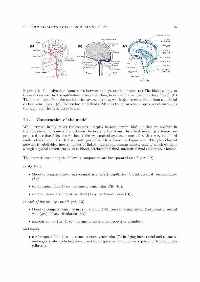
2.1. MODELING THE EYE-CEREBRAL SYSTEM 35
(a)$ (b)$ (c)$
Figure 2.1: Fluid dynamic connections between the eye and the brain: (a) The blood supply tothe eye is secured by the ophthalmic artery branching from the internal carotid artery [Eyeb]; (b)The blood drains from the eye into the cavernous sinus, which also receives blood from superficialcortical veins [Eyec]; (c) The cerebrospinal fluid (CSF) fills the subarachnoid space which surroundsthe brain and the optic nerve [Eyea].
2.1.1 Construction of the model
We illustrated in Figure 2.1 the complex interplay between several biofluids that are involved inthe fluid-dynamic connections between the eye and the brain. In a first modeling attempt, weproposed a reduced 0d description of the eye-cerebral system, connected with a very simplifiedmodel of the body, the electrical analogue of which is shown in Figure 2.2. The physiologicalnetwork is subdivided into a number of linked, interacting compartments, each of which containsa single physical constituent, such as blood, cerebrospinal fluid, interstitial fluid and aqueous humor.
The interactions among the following components are incorporated (see Figure 2.2):
in the brain:
• blood (3 compartments: intracranial arteries (I), capillaries (C), intracranial venous sinuses(S));
• cerebrospinal fluid (1 compartment: ventricular CSF (F));
• cerebral tissue and interstitial fluid (1 compartment: brain (B));
in each of the two eyes (see Figure 2.3):
• blood (5 compartments: retina (r), choroid (ch), central retinal artery (cra), central retinalvein (crv), ciliary circulation (cl));
• aqueous humor (ah) (1 compartment: anterior and posterior chamber);
and finally
• cerebrospinal fluid (1 compartment: extra-ventricular (T) bridging intracranial and extracra-nial regions, also including the subarachnoid space in the optic nerve posterior to the laminacribrosa).
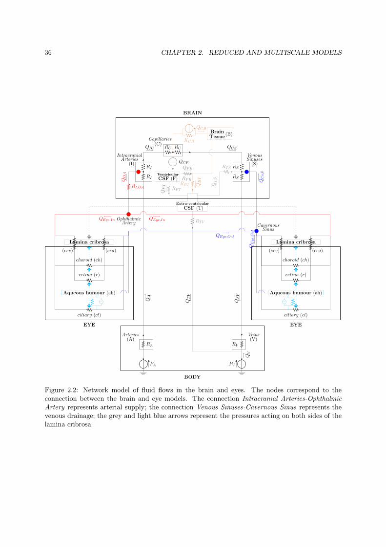
36 CHAPTER 2. REDUCED AND MULTISCALE MODELS
PA
RA
PV
RV
QCF
RI
RI
RC RC
RS
RS
RFT
RTS
RBT
RFB
RTV
KCB
VentricularCSF (F)
Extra-ventricular
CSF (T)
BrainTissue(B)
IntracranialArteries
(I)
Capillaries(C)
VenousSinuses(S)
QCB
QFB
QBT
QCSQIC
QTS
QFT
QOA
QEye,In QEye,In
QCvS
QEye,Out
QEye,Out
OphthalmicArtery
RI,OA
CavernousSinus
BRAIN
Arteries(A)
Veins(V)
BODY
Lamina cribrosa
ciliary (cl)
choroid (ch)
retina (r)
(cra)(crv)
Aqueous humour (ah)
EYE
Lamina cribrosa
ciliary (cl)
choroid (ch)
retina (r)
(cra)(crv)
Aqueous humour (ah)
EYE
QA
QTV
QSV
QV
Figure 2.2: Network model of fluid flows in the brain and eyes. The nodes correspond to theconnection between the brain and eye models. The connection Intracranial Arteries-OphthalmicArtery represents arterial supply; the connection Venous Sinuses-Cavernous Sinus represents thevenous drainage; the grey and light blue arrows represent the pressures acting on both sides of thelamina cribrosa.

2.1. MODELING THE EYE-CEREBRAL SYSTEM 37
LAMINA CRIBROSA(PLC)
OphthalmicArtery
PEye,In
Pcra,in
Pcra,1
Pcra.2
Pcra,3
Pcra,4 Pr,a Pr,c Pr,v Pcrv,1
Pcrv,out
Rcra,in
Rcra,1
Rcra,2
Rcra,3
Rcra,4
Rr,a1 Rr,a2 Rr,c1 Rr,c2Rr,v1 Rr,v2
Rcrv,1
Rcrv,2
Rcrv,3
Rcrv,4
Rcrv,out
Pcrv,2
Pcrv,3
Pcrv,4
CavernousSinus
PEye,Out
CentralRetinalArtery
CentralRetinal
Vein
Pch,in Pch,a Pch,c Pch,v
Rch,in Rch,a1Rch,a2 Rch,c1Rch,c2Rch,v1Rch,v2 Rch,out
Pch,out
Pcl,in Pcl,a Pcl,c Pcl,v
Rcl,in Rcl,a1 Rcl,a2 Rcl,c1 Rcl,c2Rcl,v1 Rcl,v2 Rcl,out
Pcl,out
Lin
JsecrIOP Rtm Episcleral
Veins
Pevp
Ruv
1
2
3
4 5
QEye,in Qch
Qcl
Qr
QEye,outQch
Qcl,v
Qr
Juf
Jah
Juv
Jtm
Figure 2.3: Network model for the eye vasculature (black portion) and aqueous humor productionand drainage (blue portion). The vasculature comprises circulation of blood in retinal, ciliary andchoroidal vascular bed. Variable resistances are marked with arrows.

38 CHAPTER 2. REDUCED AND MULTISCALE MODELS
To reflect the fluid dynamic connections between the eye and the brain, the models are coupledthrough the following relations:
• the node corresponding to the ophthalmic artery (OA) pressure in the eye model (denotedPEye,in in Figure 2.2) is connected to the intracranial arterial pressure in the brain model (PI)through an effective vascular resistance (RI,OA);
• the node corresponding to the cavernous sinus pressure (PEye,out) and that corresponding tothe episcleral venous pressure (Pevp) in the eye are directly connected to the venous sinuspressure in the brain model (PS);
• the lamina cribrosa is acted upon by the IOP from the ocular side (light blue arrow) and bythe CSF pressure in the subarachnoid space in the optic nerve, here assumed to be equal tothe extraventricular CSF pressure (grey arrow).
The flow is driven by the following mechanisms:
• the pressure drop between the central arteries (PA) and the central veins (PV );
• the active secretion of aqueous humor in the eye (Jsecr);
• the production of CSF in the brain (QCF ).
Remark 2.1.1. In this work we focus on steady simulations, neglecting, in particular, time varia-tions occurring on the time scale of heart beat. We also neglect autoregulation mechanisms of smallvessels, since we wish to keep the model relatively simple in order to understand its basic behavior.
By writing the Kirchoff law of currents at the circuit nodes, we obtain a set of nonlinear algebraicequations. The nonlinearity is a consequence of the fact that, in some compartments, resistances areassumed to depend on the pressures. Following [Gui+14] and [Ped80], we model these deformabletubes as Starling resistors, reflecting the physiological high collapsibility of these vessels when thetransmural pressure becomes negative. All constitutive laws are listed in Table 2.2, and two maintypes of flows are included in the model: filtration and pressure-driven flows. See for more detailson the mathematical modeling approach Section 2.2.1. Precise values for model parameters, the fullset of notations and the validation procedure are available in the complete version of the paper.
We are not aware of works in which a mathematical model describing the complex relationshipbetween different biofluids in the brain and in the eye in such a detailed manner has been proposed.The lumped parameter circuit for the brain stems from [LS08], where a mathematical model wasemployed for microgravity simulations. The eye model originates from [Gui+14] for the retinalcirculation and has been extended to account for the three ocular vascular beds (retina, choroidand ciliary body) adapting work from [Kie+11]. Finally, ocular hemodynamics is coupled withthe aqueous humor dynamics, as modeled in [21] and extended in [14]. The advantage of this newnetwork-based model is that it provides a systemic view, able to capture the overall dynamics ofthe interwoven physiology of blood, CSF, ocular humors and interstitial fluids in the eye and inthe brain, while maintaining a relatively accessible mathematical complexity and low computationalcosts.

2.1. MODELING THE EYE-CEREBRAL SYSTEM 39
Constitutive Relations
Brain
Cerebral Blood Flow QIC = (PI − PC)/(RI +RC)QCS = (PC − PS)/(RC +RS)
Cerebrospinal and QCB = KCB [(PC − PB)− σCB(πC − πB)]Interstitial Fluid Flow QBT = (PB − PT )/RBT
QFT = (PF − PT )/RFT
QTS = (PT − PS)/RTS
Eye
Blood Flow Qcl = (PEye,In − Pcl,c)/(Rcl,in +Rcl,a1 +Rcl,a2 +Rcl,c1)Qcl,v = (Pcl,c − PEye,Out)/(Rcl,c2 +Rcl,v1 +Rcl,v2 +Rcl,out)Qch = (PEye,In − PEye,Out)/(Rch,in +Rch +Rch,out)Qr = (PEye,In − PEye,Out)/(Rcra,in +Rcra +Rr +Rcrv +Rcrv,out)Rch = Rch,a1 +Rch,a2 +Rch,c1 +Rch,c2 +Rch,v1 +Rch,v2
Rcra = Rcra,1 +Rcra,2 +Rcra,3 +Rcra,4
Rr = Rr,a1 +Rr,a2 +Rr,c1 +Rr,c2 +Rr,v1 +Rr,v2
Rcrv = Rcrv,1 +Rcrv,2 +Rcrv,3 +Rcrv,4
Ri,v1 = Ri,v2 =
�αi (1 + (Pi,v − IOP)/(kp,ikL,i))
−4 ifPi,v > IOP
αi (1− (Pi,v − IOP)/kp,i)4/3 ifPi,v ≤ IOP
for i = cl, ch, r
αi = 8πµLi/A2i for i = cl, ch, r
kp,i = Eih3iπ
3/2/(12(1− ν2i )A3/2
i ) for i = cl, ch, rkL,i = 12Ai/(πh
2i ) for i = cl, ch, r
Rcra,n = αcra,n (1 +ΔPcra,n/(kp,cra,nkL,cra,n))−4 for n = 1, 2, 3, 4
ΔPcra,1 = (Pcra,in + Pcra,1)/2− PLC
ΔPcra,2 = (Pcra,1 + Pcra,2)/2− PLC
ΔPcra,n = (Pcra,n−1 + Pcra,n)/2− IOP, n = 3, 4αcra,n = 8πµLcra,n/A2
cra,n for n = 1, 2, 3, 4
kp,cra,n = Ecra,nh3cra,nπ
3/2/(12(1− ν2cra,n)A3/2
cra,n) for n = 1, 2, 3, 4kL,cra,n = 12Acra,n/(πh
2cra,n) for n = 1, 2, 3, 4
Rcrv,n =
�αcrv,n (1 +ΔPcrv,n/(kp,crv,nkL,crv,n))
−4 ifΔPcrv,n > 0
αcrv,n (1−ΔPcrv,n/kp,crv,n)4/3 ifΔPcrv,n ≤ 0
for n = 1, 2, 3, 4
ΔPcrv,n = (Pcrv,n + Pcrv,n+1)/2− IOP, n = 1, 2ΔPcrv,3 = (Pcrv,3 + Pcrv,4)/2− PLC
ΔPcrv,4 = (Pcrv,4 + Pcrv,out)/2− PLC
αcrv,n = 8πµLcrv,n/A2crv,n for n = 1, 2, 3, 4
kp,crv,n = Ecrv,nh3crv,nπ
3/2/(12(1− ν2crv,n)A3/2
crv,n) for n = 1, 2, 3, 4kL,crv,n = 12Acrv,n/(πh
2crv,n) for n = 1, 2, 3, 4
Aqueous Humor Flow Juf = Lin[(Pcl,c − IOP)− σpΔπp]Juv = IOP/Ruv
Ruv = (k2 + IOP)/k1Jtm = (IOP− Pevp)/Rtm
Rtm = R0(1 + κ(IOP− Pevp))
Body-Brain-Eye Coupling
QA = (PA − PI)/(RA +RI)QSV = (PS − PV )/(RS +RV )QTV = (PT − PV )/RTV
QOA = (PI − PEye,In)/RI,OA
PEye,Out = PS
Table 2.2: Summary of the model constitutive relations.

40 CHAPTER 2. REDUCED AND MULTISCALE MODELS
2.1.2 Microgravity conditions modeling and numerical results
Understanding how microgravity conditions affect ocular and cerebral fluid-dynamics and the rolethat the vascular components may play in the (potentially permanent) loss of visual acuity afterspace flight is a challenging issue. This problem is called Visually Impairment and IntracranialPressure (VIIP) syndrome [NMM14]. As part of several clinical and research projects directed inthe International Space Station, NASA recently initiated an extended acquisition campain to ana-lyze and identify astronaut-specific anatomical and physical factors that may contribute to increasethe risk of developing VIIP during long-duration space flights. Many factors are hypothesized tocontribute to VIIP, among which upper body fluid shift, alterations in intraocular pressure, in-tracranial pressure, tissue biomechanics and blood flow. Due to the difficulty to single out eachof these factors using in-vivo studies, we proposed a complementary approach, based on the novelmathematical model described in the previous section, to evaluate the interactions between fluidflows and pressures in the brain and eyes and their mechanical implications in VIIP.
To our knowledge little work has been done concerning the mathematical modeling of VIIP.The work [Nel+13] presented a lumped-parameter model to calculate mean ICP, IOP and bloodflows in the eye in zero gravity conditions. However, in the authors’ model, the eye is treated in asimplified manner, as a distensible compartment inside of which a second distensible compartmentexists, representing the intraocular vasculature. The contribution [Ver+15] developed a lumped-parameter model of fluid transport in the central nervous system aimed at simulating the influenceof microgravity on ICP. As a forthcoming step, the authors’ intention is to couple this model tolumped parameter and finite element models of the eye.
We performed simulations using the model described in Section 2.1.1 in four conditions, consid-ered to be relevant in VIIP [LS08], for different imposed blood/aqueous and blood/brain osmoticpressure differences Δπ:
• LHDT (long term head down tilt, a ground-based experimental procedure that is used tosimulate the effects of microgravity on the cardiovascular system): we account for a smallgravitational effect, which increases the central venous and arterial pressures;
• M0 (microgravity with an intact blood/brain barrier): we set the gravitational contributionand the central venous pressure equal to zero;
• M1, M2 (microgravity with a weakened blood/brain barrier): in addition to the previous case,we also increase the permeability of the blood/brain barrier by a factor 1.75 in the case M1and by a factor 2 in the case M2.
As an illustration, we present in Figure 2.4 the results of simulations for IOP, ICP and com-pressive stress in the lamina in the four simulated cases; they show that a decrease in Δπ leads to:(i) an approximately linear increase in ICP, more marked if the blood/brain barrier is weakened,as in [LS08]; (ii) a nonlinear increase in IOP, due to the venous collapse as the transmural pressurebecomes negative. Simulated ocular blood flow Figure 2.5 shows that, as Δπ decreases: (i) ciliaryand choroidal blood flows decrease almost linearly, until vessel collapse occurs, and then do so muchmore rapidly; (ii) choroidal circulation the flux in the retina initially grows owing to a purely per-fusion control mainly enacted by the intraocular venous segments.
Conclusions and perspectives. From the clinical viewpoint, these results showed interestingfeatures. Specifically, when simulating microgravity conditions, the model predicted that: (i) the
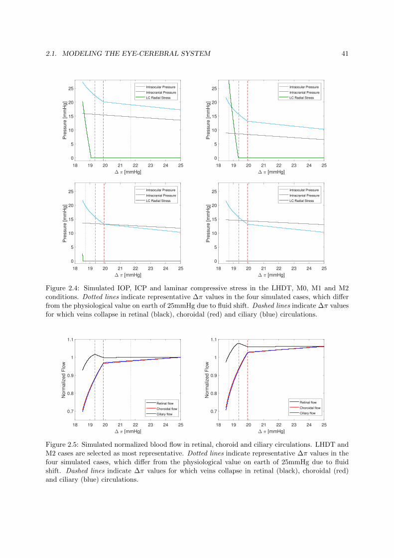
2.1. MODELING THE EYE-CEREBRAL SYSTEM 41
18 19 20 21 22 23 24 25
[mmHg]
0
5
10
15
20
25
Pre
ssu
re [
mm
Hg
]
Intraocular Pressure
Intracranial Pressure
LC Radial Stress
18 19 20 21 22 23 24 25
[mmHg]
0
5
10
15
20
25
Pre
ssu
re [
mm
Hg
]
Intraocular Pressure
Intracranial Pressure
LC Radial Stress
18 19 20 21 22 23 24 25
[mmHg]
0
5
10
15
20
25
Pre
ssu
re [
mm
Hg
]
Intraocular Pressure
Intracranial Pressure
LC Radial Stress
18 19 20 21 22 23 24 25
[mmHg]
0
5
10
15
20
25
Pre
ssu
re [
mm
Hg
]
Intraocular Pressure
Intracranial Pressure
LC Radial Stress
Figure 2.4: Simulated IOP, ICP and laminar compressive stress in the LHDT, M0, M1 and M2conditions. Dotted lines indicate representative Δπ values in the four simulated cases, which differfrom the physiological value on earth of 25mmHg due to fluid shift. Dashed lines indicate Δπ valuesfor which veins collapse in retinal (black), choroidal (red) and ciliary (blue) circulations.
18 19 20 21 22 23 24 25
[mmHg]
0.7
0.8
0.9
1
1.1
No
rma
lize
d F
low
Retinal flow
Choroidal flow
Ciliary flow
18 19 20 21 22 23 24 25
[mmHg]
0.7
0.8
0.9
1
1.1
No
rma
lize
d F
low
Retinal flow
Choroidal flow
Ciliary flow
Figure 2.5: Simulated normalized blood flow in retinal, choroid and ciliary circulations. LHDT andM2 cases are selected as most representative. Dotted lines indicate representative Δπ values in thefour simulated cases, which differ from the physiological value on earth of 25mmHg due to fluidshift. Dashed lines indicate Δπ values for which veins collapse in retinal (black), choroidal (red)and ciliary (blue) circulations.

42 CHAPTER 2. REDUCED AND MULTISCALE MODELS
venous segments play a fundamental role in controlling pressures and fluxes in the ocular circulation,owing to the possibility of their collapse; (ii) IOP and ICP increase in microgravity conditions, buttheir respective trends may be different; (iii) retinal circulation is less susceptible to microgravity-induced alterations than that in choroid and ciliary. These findings aid VIIP understanding, in-dicating that clinical assessment of ocular venous function may be considered as a determinantfactor, for which astronauts could be screened on earth and in-flight. We finally remark that theingredients embedded in the proposed model make it a very flexible tool to study interactions be-tween the eyes and the rest of the body (particularly the brain). Thus, besides the applicationto VIIP, we believe that the model could serve as a framework on which more can be built andcould be easily extended to study other pathological states, such as glaucoma (see also Section 2.2.1).
From the mathematical modeling standpoint, the outcome of this study is the first mathematicaldescription of the biophysical connection between the eye and the brain. The model was imple-mented in the open-source modeling and simulation environment OpenModelica [Ope] and validatedagainst clinical data. Next steps include (i) a sensitivity analysis study to theoretically identify sys-temic, ocular and cerebral parameters, in the spirit of our recent contributions [14; 21] and (ii) theextension of the model to the time-dependent case. The major challenge of the latter is the stronglynonlinear multiscale temporal nature of the problem, that in addition to the nonlinearities comingfrom the constitutive laws will call for well suited numerical methods for highly stiff nonlinear ODEsystems.
2.2 A zoom on mathematical models for the aqueous humor
We present in this section our work on mathematical models for the aqueous humor dynamics andtheir coupling with ocular hemodynamics, as part of the complex eye-cerebral model described inSec. 2.1. The aqueous humor is a transparent, gelatinous fluid similar to plasma located in theanterior and posterior chambers of the eye. The balance between production and drainage of aque-ous humor regulates the fluid pressure inside the eye, also known as intraocular pressure (IOP).Elevated IOP is clinically referred to as ocular hypertension and it represents a major risk factorfor irreversible vision loss, as in glaucoma. However, the establishment of optimal IOP levels forpatients is still controversial, as recently reviewed in [Ver+16]: clinical studies report evidence ofdisease progression despite a significantly reduced IOP level and optical nerve damage and visionloss despite normal IOP level. Therefore, understanding what is the relative contribution of eachrisk factor and/or different combination of risk factors is of major importance. Another meaningfulopen question is related to what determines the efficacy of IOP-lowering medications. To date,this is the only modifiable risk factor [Ver+16]. However, efficacy varies among individuals,e.g: thelowering effect is more significant when IOP is higher and it changes depending on the time of day,but the underlying mechanisms are not yet fully understood.
Motivated by these considerations, we present in Section 2.2.1 a mathematical model that de-scribes the steady state value of IOP under uncertainty. We subsequently performed numericalsimulations based on this model to assess the outcome of IOP-lowering medication used in glau-coma management. In Section 2.2.2 we further propose two increasingly complex models to coupleaqueous humor production and drainage with ocular blood circulation.

2.2. MATHEMATICAL MODELS FOR THE AQUEOUS HUMOR 43
2.2.1 Modeling the intraocular pressure under uncertainty
Only a few modeling works have studied aqueous humor flow and its relation to IOP-lowering med-ications, e.g. [LMS07; Kie+11]. Importantly, none of them explicitly accounted for uncertaintiesand variabilities in the model parameters. We proposed in [21] a simplified mathematical modeldescribing the balance between aqueous humor production and drainage; we then performed a sen-sitivity analysis aimed at quantifying the influence of parameters’ variations on the IOP distributionin various situations of clinical interest. Preliminary findings on this topic were published as peer-reviewed conference abstracts in [7; 2].
Description of the model. The mathematical approach is based on the analogy between trans-port of mass and flow of an electric current. We give hereafter the main steps in the derivation ofthe model, as an illustrative simple example of our approach when constructing lumped-parametermodels for this type of biological problems and how different phenomena were incorporated. Thenetwork-based view is schematized in Figure 2.3 (blue portion).
Aqueous humor is produced at the level of the ciliary body by a combination of a passive mech-anism, the ultrafiltration, and an active mechanism, the ionic secretion, and is modulated by thetotal inflow facility L [LMS07; Kie+11]. Here the term facility indicates hydraulic conductance,namely a flow rate per units of pressure. The ultrafiltration from the ciliary circulation consists offlow of transparent fluid across semipermeable membranes and is driven by blood/aqueous humordifferences in hydrostatic pressures (cBP−IOP ) and oncotic pressures Δπp: the latter is modulatedby a protein reflection coefficient σp. The notation cBP stands for the blood pressure in the capil-laries of the ciliary body. The inflow, as a result of the active ionic secretion, is proportional to theblood/aqueous humor osmotic pressure difference Δπs, via a reflection coefficient for low-molecularcomponents σs.
The drainage of aqueous humor from the eye is driven by passive mechanisms through two dif-ferent pathways. The trabecular pathway, also known as conventional pathway, consists of aqueoushumor flow through the trabecular meshwork, into the Schlemms canal and the episcleral veins. Asproposed in [Bru75], the model consists of a flow through a nonlinear resistor positioned betweenthe anterior chamber (where pressure is equal to IOP) and the episcleral veins (where pressure isequal to EVP), with outflow facility depending on R0 (resistance when IOP equals EVP) and Q, anoutflow obstruction coefficient. The uveoscleral pathway, also known as the non-conventional path-way, consists of aqueous humor flow through the ciliary muscle and into the supraciliary space. Thiscontribution is modeled as the flow through a nonlinear resistor connected to the ground [Kie+11],with an outflow facility depending nonlinearly on the pressure through the Michaelis-Menten typerelation [JG11]. The constant k1 is the maximum value attainable by the uveoscleral flow rate andk2 is the Michaelis constant for the uveoscleral flow rate, namely the pressure value for which theuveoscleral flow rate is half of k1.
Consequently, the steady state value of IOP, resulting from the balance between production anddrainage of aqueous humor can be written as:
L[(cBP−IOP )−σpΔπp−σsΔπs] =1
R0[1 +Q(IOP − EV P )](IOP−EV P )+
k1k2 + IOP
IOP. (2.1)
This is a scalar third-order polynomial equation in the sole unknown and can be explicitly com-puted from the previous formula. Control state values for the parameters and more details on the

44 CHAPTER 2. REDUCED AND MULTISCALE MODELS
derivation of the model can be found in [21].
To include potential sources of uncertainties as well as to identify and rank parameters hav-ing the most important influence on IOP, we applied a global stochastic sensitivity analysis to themodel described above. We considered stochastic variations in cBP following a normal distribution,and in L, Δπs, C0 = 1
R0(trabecular outflow facility), k1 and EVP following a uniform distribu-
tion, both within physiological ranges. By using the probability distribution of IOP, we computedvariance-based sensitivity indexes, also known as Sobol indexes [Sob93] and the probability densityfunction [Sap06] which describes the relative frequency of a given IOP value. For each parameter,its direct influence on is quantified in terms of first-order Sobol indexes, and the influence throughinteractions with other parameters is identified by means of the total Sobol indexes. The valuesof first-order and total indexes can be estimated via Monte Carlo simulations [Sob93] or via re-duced order models using polynomial chaos expansion [Sud08]. The former method is very costlyfrom the computational viewpoint as it requires many evaluations to ensure convergence, whereasthe latter requires considerably less evaluations. Both methods have been compared and providesimilar results. We report in the sequel the results obtained using the polynomial chaos reducedmodel. Computations were performed using Matlab/Octave and the open-source software platformOpenTURNS [Bau+16].
Numerical results and discussion. The model was used to compute the distribution in fourdifferent cases of clinical interest: (i) ocular normotensive healthy subjects (ONT); (ii) ocular hy-pertensive subjects (OHT); (iii) ONT subjects treated with IOP-lowering medications (ONTm);and (iv) OHT subjects treated with IOP-lowering medications (OHTm).
We only report here the results for the first category (healthy individuals), that also validate themodel by comparison with experimental results, see Figure 2.6. The probability density function(left panel) fits a right-skewed Gaussian curve with a frequency peak of 25% at 15.13 mmHg and askewness of 0.2, which is in a very good agreement with the results from a population-based studyon approximately subjects 12.000 subjects [Car+84] (green curve in Figure 2.6, left panel). Theresults for the Sobol indexes (Figure 2.6, right panel) suggest that IOP is strongly influenced bycBP and and Δπs and mildly influenced by the levels of L, C0 and EV P . The influence of k1 onIOP appears to be minimal.
The outcomes of the simulations in the other three cases are discussed in detail in [21]. To sum-marize, the proposed model suggests that the outcomes of IOP-lowering treatments depend on theinitial IOP level of the patient and on its individual clinical condition. Our analysis also suggeststhat IOP-lowering effects are more pronounced when aqueous humor production is affected ratherthan aqueous humor drainage. The effects of lowering IOP are also more apparent when trabecularoutflow is increased instead of the uveoscleral outflow. Another interesting finding of our analysis isthat a patients blood pressure strongly influences the outcomes of IOP-lowering treatments, whichmay explain why the effect of some drugs differ between day-time and night-time and/or amongstindividuals.
Conclusions and perspectives. Elevated IOP is a recognized risk factor for vision loss. Nu-merous risk factors are suggested in the literature [Ver+16]: age, gender, ethnicity, genetic factors,vascular dysregulation, diabetes, blood pressure etc. However, the establishment of optimal IOPlevels for patients is still controversial and what is the relative contribution of each risk factor and/ordifferent combination of risk factors is still not well understood. We proposed a mathematical modelto theoretically investigate the relationship between several uncertain parameters influencing the
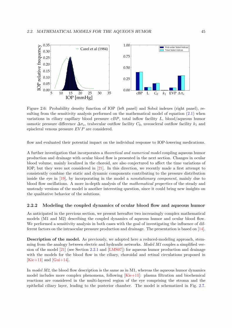
2.2. MATHEMATICAL MODELS FOR THE AQUEOUS HUMOR 45
� �� �� �� �� �� ��
������������
����
����
����
����
����
����
����
����������������
������
− Carel et al (1984)
IOP [mmHg]5 10 15 20 25 30 35
IOP
rela
tive
freq
uenc
y
0.00
0.05
0.10
0.15
0.20
0.25
0.30
0.35
��� ���
�� �
� ��� ���
����
����
����
����
����
�������������������������
�������������������
cBP L C0 k1 EVP Δπs0.00
0.25
0.50
0.75
1.00
Figure 2.6: Probability density function of IOP (left panel) and Sobol indexes (right panel), re-sulting from the sensitivity analysis performed on the mathematical model of equation (2.1) whenvariations in ciliary capillary blood pressure cBP , total inflow facility L, blood/aqueous humorosmotic pressure difference Δπs, trabecular outflow facility C0, uveoscleral outflow facility k1 andepiscleral venous pressure EV P are considered.
flow and evaluated their potential impact on the individual response to IOP-lowering medications.
A further investigation that incorporates a theoretical and numerical model coupling aqueous humorproduction and drainage with ocular blood flow is presented in the next section. Changes in ocularblood volume, mainly localized in the choroid, are also conjectured to affect the time variations ofIOP, but they were not considered in [21]. In this direction, we recently made a first attempt toconsistently combine the static and dynamic components contributing to the pressure distributioninside the eye in [19], by incorporating in the model a nonstationary component, mainly due toblood flow oscillations. A more in-depth analysis of the mathematical properties of the steady andunsteady versions of the model is another interesting question, since it could bring new insights onthe qualitative behavior of the solutions.
2.2.2 Modeling the coupled dynamics of ocular blood flow and aqueous humor
As anticipated in the previous section, we present hereafter two increasingly complex mathematicalmodels (M1 and M2) describing the coupled dynamics of aqueous humor and ocular blood flow.We performed a sensitivity analysis in both cases with the goal of investigating the influence of dif-ferent factors on the intraocular pressure production and drainage. The presentation is based on [14].
Description of the model. As previously, we adopted here a reduced-modeling approach, stem-ming from the analogy between electric and hydraulic networks. Model M1 couples a simplified ver-sion of the model [21] (see Section 2.2.1 and [LMS07]) for aqueous humor production and drainagewith the models for the blood flow in the ciliary, choroidal and retinal circulations proposed in[Kie+11] and [Gui+14].
In model M2, the blood flow description is the same as in M1, whereas the aqueous humor dynamicsmodel includes more complex phenomena, following [Kie+11]: plasma filtration and biochemicalreactions are considered in the multi-layered region of the eye comprising the stroma and theepithelial ciliary layer, leading to the posterior chamber. The model is schematized in Fig. 2.7.

46 CHAPTER 2. REDUCED AND MULTISCALE MODELS
Enforcing the Kirchhoff Current Law at each node of the circuit, except where given data areassumed and where connection to ground is applied, one obtains a nonlinear system of algebraicequations in the unknown vector
P =�Cst, Caq, P
cilc , Pst, Pant, Ppost, mbl, P
O2c , PO2
v , PO2ce , PO2
aq
�T, (2.2)
where Cst and Caq are the protein concentrations in the stroma and in the aqueous humor, P cilc is
the blood pressure in the ciliary body capillaries, Pst, Ppost and Pant are the aqueous humor pres-sures in the stroma and in the posterior and anterior chambers, mbl basolateral ionic concentration,and PO2
c , PO2v , PO2
ce , PO2aq are the partial pressures of oxygen in the ciliary body capillaries, veins,
epithelium and aqueous humor.
��������
��������
���������
���������
��������
��������
���������
���������
��������
��������
���������
���������
����������������
��������������������
������������
������������
��������
��������
���������
���������
G1 G
2
I1
Iprot
out
Gc G
ce
I2
Ipl
onc
Ionc
aq
Ibl
Ius
Ipump
Irem
IO2
IO2
cv
IO2
v,out
Ifilt,c
QO2
ce
prod,ce
QO2
lens
I
Iaq
out
O2
ac
Pa
PO2
c
PO2
v
PO2
ce PO2
aq
Pst
PEVP
Pc
cil
mplm
bl
Cpl
CstC
aq
Gfac
GiopGst
Gbl
Ibl
antP
Ppost
Figure 2.7: Equivalent electrical circuit for aqueous humor production and drainage. Each node ofthe circuit (black bullet) is connected to another node either through a conductance (denoted by thesymbol G) or through a current source (denoted by a rhombus or by a circle). The nodal quantitiesindicated by P (capital letter) represent a pressure (in mmHg). The nodal quantities indicated byC (capital letter) represent a concentration (in gml−1) while those indicated by m (small letter)represent a molar concentration (in µmolml−1). The quantities surrounded by a box are assumedto be given values defined by the user. The current sources I1 and I2 are fixed values while the othercurrent sources are controlled by the drop of the two nodal values across which they are located orby the drop of the two nodal values to which they are connected by the dashed arrows. The verticalshaded triangle symbol represents connection of the considered network branch to ground.
Thus, the overall models M1 or M2 consists in two main blocks, one for the aqueous humor flowand one for blood flow, which are strongly coupled, since: (i) the blood pressure in capillaries and

2.2. MATHEMATICAL MODELS FOR THE AQUEOUS HUMOR 47
0 20 40 60 80 100 120 140 160 180 20010
10.5
11
11.5
12
12.5
13
13.5
14
14.5
% change in AH outflow
pre
ssu
re [
mm
Hg
]
P vitreous
P anterior
P stroma
0 20 40 60 80 100 120 140 160 180 2000.99
1
1.01
1.02
1.03
1.04
1.05
1.06
% change in AH outflow
no
rma
lize
d p
ressu
re [
−]
P vitreous
P anterior
P stroma
Figure 2.8: Sensitivity analysis as a function of percentage change in DAH . Stromal and anteriorchamber pressures are influenced by variations in aqueous humor drainage, while intraocular pres-sure is influenced in a milder manner. Each pressure tends to a saturation value as drainage isincreased. A red square indicates the baseline value for each pressure.
veins contributes to regulate production and drainage of aqueous humor, and (ii) the aqueous hu-mor pressure acts as an external pressure on the blood vessels thereby altering blood flow. For thesolution of the overall problem a block fixed point iteration is adopted until convergence.
Numerical results. Computations of the first order Sobol indexes [Sob93] based on M1 confirmed,as in [21], that acting on the aqueous humor inflow seems more effective than changing aqueoushumor outflow. In addition, regarding hemodynamic aspects, simulations showed that pressure inciliary capillaries and retinal blood flow are strongly influenced by blood pressure and systemicvascular resistance, which are systemic factors depending on the general condition of the individual.
We also performed a sensitivity analysis on model M2, but only in a deterministic framework.Because of the increased complexity of the formulation, a self-consistent coupling with the bloodflow model was not addressed in a preliminary validation, and computations were performed byassuming the dependent variables P cil
c , PO2c and PO2
v in (2.2) to be given quantities. In particu-lar, we focused our attention in the computation of Pst and Pant (Ppost is assumed to be equal toPant), and of the pressure Pvitreous in the vitreous which coincides with the intraocular pressure.Simulations were run to evaluate the dependence of these three variables on the variation (i) ofthe production of aqueous humor PAH and (ii) of the total aqueous humor drainage DAH . A com-plete description of the parameters and results is available in [14]. As an illustration, we reportin Figure 2.8 the outcomes of the simulations in the case where the drainage of aqueous humorDAH is varied. Results show that the intraocular pressure is less sensitive to parameter variation,unlike stromal and anterior chamber pressures. In particular, we see that, as physically expected,these latter pressures decrease appreciably as DAH becomes larger. However, results clearly re-veal that a further increase of drainage has no positive effect on pressure decay. This is reflectedinto a saturation of all the pressure curves to a limit value, as visible in the right panel of Figure 2.8.
Discussion and perspectives. The mathematical models M1 and M2, coupling aqueous humorproduction and drainage with ocular blood flows, lead to a better understanding of the delicate,yet important, relationship between different factors determining intraocular pressure. Further on,this theoretical investigation helped in identifying patients-specific factors (as for instance systemic

48 CHAPTER 2. REDUCED AND MULTISCALE MODELS
blood pressure) that influence the efficacy of different medications used in glaucoma management.The complex multi-physical nature of this coupled dynamics called in a first approximation for sev-eral simplifications: the model is steady and does not account for autoregulation mechanisms insmall vessels. In this direction, the aqueous humor block could incorporate a nonstationary com-ponent as we recently proposed in [19]; as for the ocular blood flow contribution, time-dependentmodels including autoregulation in the retina, with different levels of complexity, are developed in[Gui+14; AGL16] and could be coupled with the first block. From the mathematical viewpoint,taking into account the different nonlinearities due to autoregulation phenomena raises new inter-esting questions both at the theoretical and computational level; another challenge comes from theunderstanding of the unsteady component of the system and its asymptotic behavior.
A different development was triggered by recent discussions with A. Mauri and R. Sacco, that aimsat coupling the current model that describes aqueous humor dynamics at the ocular tissue scalemodel (coarse level) to an epithelial cellular scale model (fine level). More precisely, the idea isto keep the description of the drainage path and of the ultrafiltration process at a macroscopiclevel and to expand the model of the ionic pump at the fine level in the spirit of the recent modelproposed by my colleagues and their collaborators in [Mau+16]. Such an approach would hopefullyprovide insights in understanding the role of the sodium-potassium pump as an important playerin the aqueous humor production, not only at the cellular level, but also at a macroscopic scale. In[Mau+16], the velocity-extended Poisson-Nernst-Planck equations describing ion electrodiffusion arecoupled to the Stokes equations to describe aqueous humor flow into the basolateral space adjacent tothe nonpigmented ephitelial cells. The coupling between this three-dimensional partial differentialequations system and the reduced 0D description of the rest of the circuit presents interestingmodeling (for boundary and interface conditions) and numerical (for the solving algorithm) issues.In particular, the new numerical approach based on a splitting procedure that we detail in the nextsection could provide a sound starting point in devising an appropriate algorithm for the problem.
2.3 A new algorithm for the numerical solving of coupleddistributed–0d problems
Many strategies have been adopted for the numerical solution of coupled PDE–ODE systems inthe context of blood flow modeling. In particular, monolithic and splitting (or partitioned) schemeshave been proposed, where the PDE and ODE systems are solved simultaneously or in separatesubsteps, respectively. An extensive discussion about their advantages and limitations can be foundin [QVV16].
The contribution presented in this section focuses on splitting techniques and on the propertiesof their modular structure. Among the many interesting contributions in this area, we mention herethose that are most closely related to our work. In [QRV01], the multiscale coupling between theNavier-Stokes equations in a rigid domain and a lumped parameter model is considered. A split-ting strategy based on subiterations between PDE and ODE solvers at each time step is proposedand assessed in different meaningful configurations. This splitting formulation was then used asan effective tool to prove the well-posedness of the coupled problem [QV03], in combination withappropriate fixed point results. In [FIGM15], the authors compare the numerical stability of ex-plicit and implicit coupling between the Stokes or Navier-Stokes equations and circuit-based modelscontaining resistances and capacitances. Unconditional stability was proved in the implicit case,whereas conditional stability was proved in the explicit case. In [Mog+13], a time implicit approachto couple general lumped parameter models with a finite-element based solution of a Navier-Stokes

2.3. NUMERICAL SOLVING OF COUPLED DISTRIBUTED–0D PROBLEMS 49
problem in a 3d domain is proposed. The algorithm combines the stability properties of monolithicapproaches with the modularity of splitting algorithms. The method is based on a Newton typeiterative scheme, where data are exchanged between the two domains at each Newton iteration ofthe nonlinear Navier-Stokes solver to ensure convergence of both domains simultaneously.
To the best of our knowledge, the splitting schemes that have been proposed for coupled PDE–ODE systems in the context of fluid flow modeling so far, require subiterations between substeps,usually involving the values of pressure and flow rate at the multiscale interfaces, in order to achieveconvergence of the overall algorithm. Depending on the mathematical properties of the models ineach substep and of the coupling between them, the convergence of such subiterations might becomean issue, especially in the case of nonlinear problems.
We describe in this section a new method, presented in [3] and detailed in a full subsequentpaper, that aims at providing a novel splitting scheme for coupled PDE–ODE systems for fluid flowthat does not require subiterations between substeps in order to achieve stability for the overallalgorithm. The stability properties of the scheme follow from ensuring that the physical energybalance is maintained at the discrete level via a suitable application of operator splitting techniquesto semi-discretize the problem in time [Glo03, Chap. II]. As a result, the proposed algorithmallows us to: (i) solve in separate substeps potential nonlinearities within the systems of PDEsand/or ODEs; (ii) maintain some flexibility in choosing the numerical method for the solution ofeach subproblem; (iii) ensure unconditional stability without the need of subiterations betweensubsteps.
2.3.1 Description of the coupled Stokes–0d problem
Geometrical architecture of the coupled system. We start by describing the main blocks thatconstitute the model under consideration. The geometrical setting of the coupled problem consistsof: (i) L regions of space denoted by Ωl ⊂ Rd, with l ∈ L = {1, . . . , L} and d = 2 or 3, where thefluid flow is described by the Stokes equations; (ii) M lumped hydraulic circuits denoted by Υm,with m ∈ M = {1, . . . ,M}, where the fluid flow is described by the hydraulic analog of the Kirchofflaws of currents and voltages. We assume that the boundary of each domain Ωl, denoted by ∂Ωl,is the union of three portions, namely
∂Ωl = Γl ∪ Σl ∪ Sl (2.3)
where different types of boundary and interface conditions are imposed. Specifically, Dirichletconditions are imposed on Γl, Neumann conditions are imposed on Σl and Stokes-circuit couplingconditions are imposed on Sl, as described below. We assume that Dirichlet conditions are imposedon a portion of the boundary of each domain Ωl, i.e. Γl �= ∅, and that each domain Ωl is connectedto (at least) one circuit, i.e. Sl �= ∅. In particular, each region Ωl may have jΩl
≥ 1 Stokes-circuitconnections, implying that each boundary portion Sl may be written as
Sl =�
m∈Ml
Slm (2.4)
with l ∈ L. We remark that, for each l ∈ L, the set Ml ⊆ M identifies the circuits Υm that areconnected to Ωl. Similarly, each circuit Υm may have jΥm ≥ 1 Stokes-circuit connections and theset Lm ⊆ L identifies the Stokes regions Ωl that are connected to Υm. We will also consider caseswhere Neumann conditions are not imposed on the boundary of Ωl, i.e. Σl = ∅, as it happensin Example 3 described below. It may also happen that the same Stokes region Ωl and the same

50 CHAPTER 2. REDUCED AND MULTISCALE MODELS
circuit Υm enjoy multiple connections. Thus, an additional subscript is introduced to distinguishbetween the various connections, so that we can write:
Slm =
jΩl,Υm�
k=1
Slm,k, (2.5)
where jΩl,Υm is the total number of connections between Ωl and Υm. Note that with these notations,we also have
jΩl=
�
m∈Ml
jΩl,Υm and jΥm =�
l∈Lm
jΩl,Υm . (2.6)
Stokes problems in Ωl. Let vl = vl(x, t) and pl = pl(x, t), for l ∈ L, denote the velocity vectorfield and the pressure field, respectively, pertaining to the fluid in each domain Ωl × (0, T ), withΩl ⊂ Rd, d = 2, 3 and T > 0. Then, for l ∈ L, we can write the Stokes equations as:
∇ · vl = 0 in Ωl × (0, T ) (2.7)
ρ∂vl∂t
= −∇pl + µΔvl + ρfl in Ωl × (0, T ) (2.8)
where ρ and µ are positive given constants representing the fluid density and dynamic viscosity,respectively, and fl are given body forces per unit of mass. The system is equipped with the initialconditions:
vl(x, t) = vl,0(x) in Ωl (2.9)
and the boundary and interface conditions:
vl = 0 on Γl × (0, T ) (2.10)�− plI + µ∇vl
�nl = −plnl on Σl × (0, T ) (2.11)
�− plI + µ∇vl
�nlm,k = glm,k on Slm,k × (0, T ) (2.12)
where I is the d× d identity tensor, nl is the outward unit normal vector to Σl, and pl = pl(t) aregiven functions of time. For m ∈ Ml and k = 1, . . . , jΩl,Υm , the vector nlm,k denotes the outwardunit normal vector to Slm,k and the functions glm,k are defined via the coupling conditions (2.15).
Lumped hydraulic circuits in Υm. Let the dynamics in each lumped hydraulic circuit Υm, form ∈ M = {1, . . . ,M}, be described by the vector ym = [ym,1, ym,2, · · · , ym,dm ]
T of state variablessatisfying the following system of (possibly nonlinear) ODE system:
dym
dt= A
m(ym, t)ym + rm(ym, t) (2.13)
equipped with the initial conditionsym(t = 0) = ym,0 (2.14)
where ym and rm are dm-dimensional vector-valued functions and Am
is a dm × dm tensor. Thetensor A
membodies topology and physics of the connections among the circuit nodes and the
vector-valued function rm comprises two contributions: (i) sources and sinks within the circuit,including generators of current and voltage; and (ii) connections with Stokes regions.
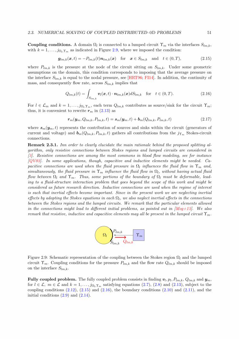
2.3. NUMERICAL SOLVING OF COUPLED DISTRIBUTED–0D PROBLEMS 51
Coupling conditions. A domain Ωl is connected to a lumped circuit Υm via the interfaces Slm,k,with k = 1, . . . , jΩl,Υm as indicated in Figure 2.9, where we imposed the condition:
glm,k(x, t) = −Plm,k(t)nlm,k(x) for x ∈ Slm,k and t ∈ (0, T ), (2.15)
where Plm,k is the pressure at the node of the circuit sitting on Slm,k. Under some geometricassumptions on the domain, this condition corresponds to imposing that the average pressure onthe interface Slm,k is equal to the nodal pressure, see [HRT96; FI14]. In addition, the continuity ofmass, and consequently flow rate, across Slm,k implies that
Qlm,k(t) =
�
Slm,k
vl(x, t) · nlm,k(x)dSlm,k for t ∈ (0, T ). (2.16)
For l ∈ Lm and k = 1, . . . , jΩl,Υm , each term Qlm,k contributes as source/sink for the circuit Υm;thus, it is convenient to rewrite rm in (2.13) as
rm(ym, Qlm,k, Plm,k, t) = sm(ym, t) + bm(Qlm,k, Plm,k, t) (2.17)
where sm(ym, t) represents the contribution of sources and sinks within the circuit (generators ofcurrent and voltage) and bm(Qlm,k, Plm,k, t) gathers all contributions from the jΥm Stokes-circuitconnections.
Remark 2.3.1. Inn order to clearly elucidate the main rationale behind the proposed splitting al-gorithm, only resistive connections between Stokes regions and lumped circuits are considered in[3]. Resistive connections are among the most commons in blood flow modeling, see for instance[QV03]. In some applications, though, capacitive and inductive elements might be needed. Ca-pacitive connections are used when the fluid pressure in Ωl influences the fluid flow in Υm and,simultaneously, the fluid pressure in Υm influence the fluid flow in Ωl, without having actual fluidflow between Ωl and Υm. Thus, some portions of the boundary of Ωl must be deformable, lead-ing to a fluid-structure interaction problem that goes beyond the scope of this work and might beconsidered as future research direction. Inductive connections are used when the regime of interestis such that inertial effects become important. Since in the present work we are neglecting inertialeffects by adopting the Stokes equations in each Ωl, we also neglect inertial effects in the connectionsbetween the Stokes regions and the lumped circuits. We remark that the particular elements allowedin the connections might lead to different initial problems, as pointed out in [Mog+13]. We alsoremark that resistive, inductive and capacitive elements may all be present in the lumped circuit Υm.
Ωl
Slm,k
Plm,k
Qlm,k
Υm
Figure 2.9: Schematic representation of the coupling between the Stokes region Ωl and the lumpedcircuit Υm. Coupling conditions for the pressure Plm,k and the flow rate Qlm,k should be imposedon the interface Slm,k.
Fully coupled problem. The fully coupled problem consists in finding vl, pl, Plm,k, Qlm,k and ym,for l ∈ L, m ∈ L and k = 1, . . . , jΩl,Υm satisfying equations (2.7), (2.8) and (2.13), subject to thecoupling conditions (2.12), (2.15) and (2.16), the boundary conditions (2.10) and (2.11), and theinitial conditions (2.9) and (2.14).

52 CHAPTER 2. REDUCED AND MULTISCALE MODELS
Remark 2.3.2. Due to the complex nonlinear structure of the fully coupled problem, to our knowl-edge, existence of solutions has been proved only for some particular cases. For example, in [QV03],the authors prove local in time existence of a solution, when the connections are made through bridg-ing regions. In [BGM10], the existence of a strong solution for small data is demonstrated, in thecase of the coupling between the Navier-Stokes problem and a single resistor.
In [3] we showed that the full coupled Stokes-0d system satisfies an energy identity that embodiesthe main mechanisms governing the physics of the system. More precisely, the analysis shows that,in the case of lumped circuits having a structure contributing to the overall energy dissipationand in the absence of external forcing terms, the energy of the full coupled problem will decay intime. This is the fundamental physical and mathematical property that we aim at preserving atthe discrete level and that provides the main rationale for our splitting scheme described below.
2.3.2 First-order splitting algorithm for the time discretization of the coupledproblem and stability analysis
Our numerical strategy is based on the operator splitting technique, see e.g. [Glo03, Chap. II],which leverages a semi-discretization in time to solve sequentially in separate substeps the PDEsystems associated with the Stokes regions and the ODE systems associated with the lumped hy-draulic circuits. The most important feature of the scheme is that the substeps are designed sothat the energy at the semi-discrete level mirrors the behavior of the energy of the full coupledsystem, thereby providing unconditional stability to the proposed splitting method. We presentnext the main steps of the algorithm; for more details about its characteristics and the imple-mentation, see [3]. We emphasize that the version of the method detailed below yields, at most,a first-order accuracy in time, since it includes only two substeps; however, the scheme can begeneralized to attain second-order accuracy using symmetrization techniques [Glo03, Chap. VI] orsuitable time-extrapolations of quantities of particular interest, in the same spirit as [Fen13; FLV15].
First-order splitting algorithm. Let Δt denote a fixed time step, let tn = nΔt and let ϕn =ϕ(t = tn) for any general expression ϕ. Let v0
l = vl,0 for all l ∈ L and y0m = ym,0 for all m ∈ M.
Then, for any n ≥ 0 solve:
Step 1 For each l ∈ L, m ∈ M and k = 1, . . . , jΩl,Υm , given vnl and yn
m, find vl and ym such that
∇ · vl = 0 in Ωl × (tn, tn+1) (2.18)
ρ∂vl∂t
= −∇pl + µΔvl + ρfl in Ωl × (tn, tn+1) (2.19)
dym
dt= bm(Qlm,k, Plm,k, t) in (tn, tn+1) (2.20)
with the initial conditions
vl(x, tn) = vn
l (x) in Ωl (2.21)
ym(tn) = ynm (2.22)
and the boundary conditions
vl = 0 on Γl × (tn, tn+1) (2.23)�− plI + µ∇vl
�nl = −plnl on Σl × (tn, tn+1) (2.24)
�− plI + µ∇vl
�nlm,k = −Plm,knl,m on Slm,k × (tn, tn+1) (2.25)

2.3. NUMERICAL SOLVING OF COUPLED DISTRIBUTED–0D PROBLEMS 53
with �
Slm,k
vl(x, tn) · nlm,k(x, t
n) dSlm,k = Qlm,k(t) in (tn, tn+1) (2.26)
and then set
vn+ 1
2l = vl(x, t
n+1), pn+1l = pl(x, t
n+1) and yn+ 1
2m = ym(tn+1). (2.27)
Step 2 For each l ∈ L, m ∈ M and k = 1, . . . , jΩl,Υm , given vn+ 1
2l and y
n+ 12
m , find vl and ym suchthat
ρ∂vl∂t
= 0 in Ωl × (tn, tn+1) (2.28)
dym
dt= A
m(ym, t)ym + sm(ym, t) in (tn, tn+1) (2.29)
with the initial conditions
vl(x, tn) = v
n+ 12
l (x) in Ωl (2.30)
ym(tn) = yn+ 1
2m (2.31)
and set
vn+1l = vl(x, t
n+1) and yn+1m = ym(tn+1). (2.32)
The stability properties of the algorithm are investigated in the next theorem. The analysis wasperformed on a simplified problem that, however, still preserves the main difficulties associated withthe coupling of PDEs and ODEs considered in this work.
Theorem 2.3.3. Consider the coupled Stokes–0d problem described in Section 2.3.1 and assumethat (i) the circuit properties are such that, for all m ∈ M, the tensor A
mis constant and B
mis positive definite, where B
mgathers all the contributions from resistive, capacitive and inductive
elements in the lumped circuits; (ii) the are no forcing terms, namely FΩ(t) = FΥ(t) = 0 for allt ≥ 0, where FΩ represents the forcing on the system due to body forces and external pressures actingon the Stokes regions and FΥ the forcing on the system due to generators of current and voltagewithin the lumped circuits, respectively; (iii) the Stokes-circuit connections are of the type describedin Section 2.3.1. Under these assumptions, the algorithm given by Steps 1 and 2 is unconditionallystable.
The key ingredient in the proof is the following: the uncoditional stability of the algorithm is a directconsequence of treating the contributions from the jΥm Stokes-circuit connections, represented bybm(Ql,m, Pl,m, t), implicitly in Step1 in Eq. (2.20) (for instance, by means of an implicit Euler schemefor the time-discretization). The coupling conditions are not disrupted, and we let the two substepscommunicate via the initial conditions. As a consequence, the proposed splitting technique does notintroduce uncontrolled artificial terms in the energy, thus ensuring the stability of the algorithm.
2.3.3 Numerical results and discussion
We evaluated the performances of the first order splitting method proposed in Section 2.3.2 on threeillustrative examples that differ by: (i) number of Stokes regions and lumped circuits; (ii) numberof connections between Stokes regions and lumped circuits; and (iii) type of elements within thelumped circuits. The equivalent electric circuits are represented in Figures 2.10, 2.11 and 2.12,

54 CHAPTER 2. REDUCED AND MULTISCALE MODELS
respectively. We derived explicit solutions for the full coupled problem in each example, againstwhich our (as well as other) numerical methods can be tested and we assessed the convergenceproperties of the method for different choices of time step, showing that the expected first-orderconvergence in time is actually achieved. The spatial discretization of the Stokes problem is handledvia a standard finite-element approach, the temporal discretization of the Stokes and 0d problems ishandled via an implicit Euler method and the computational framework relies on the finite elementlibrary Freefem [Hec12].
p1Ω1
Σ1
Γ1
Γ1
S11,1
P11,1
Q11,1
R11
y11
C11
Υ1
R12(y1, t)
y12
C12(y1, t)R13
�p1
Figure 2.10: Example 1. The two-dimensional Stokes region Ω1 is connected to the lumped circuitΥ1 via a resistive element with resistance R11.
p1Ω1
Σ1
Γ1
Γ1
S11,1
P11,1
Υ1
Q11,1
R11
y11
C11
R12 L12
y12
y13
C13
R14
R13
p
Q21,1
Ω2
S21,1
Γ2
Γ2
Σ2
P21,1p2
Figure 2.11: Example 2. The two-dimensional Stokes regions Ω1 and Ω2 are connected to thelumped circuit Υ1 via resistive elements with resistance R11 and R14, respectively.
Ω1
S11,2
Γ1
Γ1
S11,1
P11,1P11,2
Q11,1
R11,1
y11
C11
R12
p1
Q11,2
R11,2
y12
C12
R14
p2
R13 L13
y13
Υ1
Figure 2.12: Example 3. The two-dimensional Stokes region Ω1 is connected to the lumped circuitΥ1 via two resistive elements with resistance R11,1 and R11,2, respectively.

2.3. NUMERICAL SOLVING OF COUPLED DISTRIBUTED–0D PROBLEMS 55
We present the results obtained on Example 1; for Examples 2 and 3, we refer to [3]. Theycorrespond to the case of nonlinear variable resistance R12 and capacitance C12, but we also testedthe method in the case of constant R12 and C12 against the exact solution and obtained similarperformances as in the nonlinear case. Figure 2.13 displays a comparison between the exact solutionand different numerical approximations of physical quantities of interest, namely pressure P11,1 andflow rate Q11,1 at the Stokes-circuit interface S11,1 (upper panel) and pressure y11 and volumey12 in the 0d circuit (lower panel). We remark that the nonlinearities in R12 and C12 have beentreated explicitly, which means that R12 and C12 are evaluated at the previous time step. A goodagreement is obtained for P11,1, y11 and y12 for Δt = 0.01, and the error decreases as Δt is reduced.The numerical approximation of Q11,1 captures the periodicity of the solution even for Δt = 0.01,but the peaks are lower than those exhibited by the exact solution. As Δt is the reduced, thecomputed Q11,1 approaches the exact peaks of the interface flow rate, thereby capturing the fulldynamics of the problem. Figure 2.13 also shows that the numerical solution is not affected byspurious oscillations or instabilities, even for the largest time step. These findings confirm that thechoice of the time step affects the accuracy of the computed solution but not the stability of thenumerical scheme, as proved in Theorem 2.3.3.
Interface quantities
��������� ��� � ��� �
������������������
���
���
���
����
����
����
���������∆�������∆��������∆��������
��� ��� �������
����
����
��������� ��� � ��� �
�������������
�
�
�
�
�
������∆�������∆��������∆��������
��������� ��� � ��� �
����������������
���
���
���
����
����
����
���������∆�������∆��������∆��������
��� ��� ���
����
����
����
��������� ��� � ��� �
���������
���
�
���
�
��������∆�������∆��������∆��������
��� ��� ������
����
����
����
0d unknowns
Figure 2.13: Example 1. Comparison between the exact solution and the corresponding numericalapproximation for interface quantities (top) and 0d unknowns (bottom), for three time steps Δt =0.01, 0.005, 0.001, over one period once the periodicity is reached.
Recall that the time-discretization scheme is based on a first order operator splitting technique,which is known to be first-order accurate in time. We performed a standard time refinement studythat confirmed this property, as shown in Figure 2.14.

56 CHAPTER 2. REDUCED AND MULTISCALE MODELS
������������������
����
��������������������������
����
����
����
����
���
�����������������
�����������������
�����������������
(a) Example 1
������������������
����
��������������������������
����
����
����
���
�����������������
�����������������
�����������������
(b) Example 2
������������������
����
��������������������������
����
����
����
����
���
��
�����������������
�����������������
�����������������
(c) Example 3
Figure 2.14: Plot of the energy norm errors, in logarithmic scale as a function of the global timestep Δt = 0.01, 0.005, 0.001 for the three examples considered.
Perspectives. The energy-based operator splitting approach developed in [3] is based on a verysimple version of this technique, which is first-order accurate. It has the advantages of an easy imple-mentation, good stability and robustness properties, and low computational cost. This frameworkcould serve as a basis for the extension to high order methods, as briefly discussed in Section 2.3.2.The proposed algorithm allows us to associate to each block of the problem a specific operator andto solve it in separate substeps, by means of a well-suited numerical method. This feature can befurther exploited in more complex situations: (i) coupling between Navier-Stokes equations and alumped parameter model, in the Newtonian or non-Newtonian case; (ii) coupling between a modeldescribing flow in a compliant tube and a 0d appropriate model; (iii) more generally, couplingbetween different PDEs in the various Ωl, (for instance to accommodate Stokes and Darcy) andreduced models.
2.4 Conclusions and outlook
In this chapter, our strategy has been to tackle the complexity of the bio-fluid dynamics in thecoupled eye-cerebral system by means of a two-stage approach. First, we developed network-basedmodels that allow to understand the main dynamics of the system thanks to their simplified math-ematical structure and to compute average values of the unknowns at relatively low computationalcosts. They are also particularly well suited for sensitivity analysis studies to input data, that wesuccessfully used to discriminate the contribution of different factors on flow quantities. In addition,these robust mathematical models have the advantage that can be dynamically complexified andimplemented as our understanding evolves. Second, we envisioned a multiscale approach, where re-gions of interest that require the use of a detailed model are coupled to a reduced 0d description ofthe rest of the network, thus leading to a coupled PDE–ODE system. We proposed a novel techniquebased on operator splitting for the time discretization of such coupled distributed–reduced prob-lems, that allows to solve separately and sequentially each model, without the need of sub-iterations.
We selected in the sequel some possible further developments:
Towards a multi-domain and multiphysics model of the eye. To the best of our knowledge,the mathematical and computational modeling of the eye is still at its early stages, see for instance[Ale17] and the references therein. In the framework of the thesis of Lorenzo Sala, co-advised with

2.4. CONCLUSIONS AND OUTLOOK 57
Chirstophe Prud’homme (Univ. de Strasbourg) and Giovanna Guidoboni (Univ. of Missouri), wemade the first steps in constructing such a full model, in which ocular biomechanics, fluid dynamicsand hemodynamics are coupled. Currently, the system combines: (i) a circuit-based model for bloodflow in the retinal vasculature, central retinal artery and central retinal vein, as in Sections 2.1 and2.2.2; (ii) a three-dimensional porous media model for the perfusion of the lamina cribrosa and(iii) a three-dimensional isotropic elastic model for the biomechanics in the lamina cribrosa, retina,choroid, sclera and cornea. From a numerical viewpoint, the problem requires solving a poroelasticmodel for the coupling between biomechanics and hemodynamics in the lamina cribrosa, which callsfor (i) high accuracy in the approximation for both primal variables (i.e. displacement and pres-sure) and dual variables (i.e. stress and perfusion velocity), and (ii) integral boundary conditionsto account for the coupling between zero- and three-dimensional model components. To numer-ically solve the coupled system, we used a hybridizable discontinuous Galerkin method [CGL09],implemented in Feel++. Furthermore, to handle the multiscale nature of this problem, the complexcoupling has been achieved using an integral boundary condition and a time-splitting energy-basedscheme in the spirit of the method developed in Section 2.3. A collaborative effort in this sensewas presented and published as peer-reviewed conference abstracts [15; 16] and a full paper is inpreparation. Future developments will include the coupling with mathematical and computationalmodels for the cerebro-spinal fluid circulation (see also the discussion in Section 1.6), an extendedblood circulation for the whole body and a three-dimensional description of the fluid dynamics ofthe vitreous and aqueous humor.
Mathematical modeling and simulations for the brain and eye-cerebral system: a mul-tiscale approach. As already discussed in Section 1.6, it would be interesting to extend ourcontributions on the 3d models for cerebral blood flow to a multiscale framework. Eventually, the3D description of the flow would be integrated in a model of the entire circulatory system. Theadvantage of such a closed-loop model are that the artificial boundaries are not present anymoreand moreover, it could include feedback and control mechanisms. Similarly, the complexity of thecoupled eye-cerebral system calls for a multiscale modeling approach. Network-based models, as theone presented in Section 2.1, allow to capture the main dynamics and averaged behavior, whereasdetailed 3d models allow to interface with clinical data that are 3D in nature, e.g. MRA maps orOptical Coherence Tomography (OCT) images. The mathematical complexities of such a multiscaleapproach, as briefly discussed in Section 2.3, include in particular the extension to 3d geometriesand to the case of the Navier-Stokes equations. Also, such an approach requires the development offlexible, versatile and scalable computational framework, in which the multi-components/multiscale/multiphysics mathematical models can be solved numerically. Moreover, the use of adaptive androbust methods to combine computations with experimental data and measurements is necessary.These new research directions are at the core of the project thesis of Philippe Ricka, co-advisedwith Christophe Prud’homme (Univ. de Strasbourg) and Giovanna Guidoboni (Univ. of Missouri),starting from September 2017.

58 CHAPTER 2. REDUCED AND MULTISCALE MODELS

Chapter 3
Numerical strategies for coupledfluid-structure problems. Applicationsto multiphysics computational modelsin biology and medicine
Three-dimensional macro-scale fluid models can describe blood flow dynamics in large vessels (ar-teries or veins), by means of the Navier-Stokes system, as presented in Chapter 1. Alternatively,in Chapter 2 we used 0d reduced models, based on systems of ODEs describing blood flow withelectric analogy, possibly coupled with a 3d description of the flow, in a geometric multiscale ap-proach. The representation of these problems can be enriched to take into account the combinedeffects of flow and different structures, from a multiphysics perspective. In this direction, two typesof fluid-structure interaction phenomena can be considered:
• internal flows, when the external fluid boundary has an elastic part or is entirely composedof an elastic structure, e.g. a model for blood flow in arteries with deformable walls;
• internal structures, when rigid or deformable bodies float or actively move in a fluid flowplaced in a container, e.g. a mixture of plasma and red blood cells, as a model for blood at avery small scale.
In this chapter, we gather two contributions, corresponding each to one of these situations. In Sec-tion 3.1, a coupled fluid-structure interaction model from the first category is presented, based ona description of blood flow dynamics by the Navier-Stokes equations in a moving domain, coupledwith the linear elasticity equations describing the vessel wall deformation. This coupled multiphysicsmodel is subsequently utilized for simulating blood flow in the aorta, in view of a specific biomedicalapplication. The case of an internal structure, namely a rigid particle evolving passively in a fluid,is presented in Section 3.2, with an emphasis on the issue of how to handle contact with the wall ofa rigid container.
3.1 Computational modeling of blood flow in the aorta
On the basis of [20], we aim at providing in this section an example of how combining two comple-mentary studies:
59

60 CHAPTER 3. COUPLED FLUID-STRUCTURE PROBLEMS
• a 3d MRI angiography of the aorta in 30 patients after coarctation repair and
• a 3d fluid-structure computational model characterizing the fluid dynamics in the aorta (flow,pressure, and wall shear stress)
can shed some light on the causes of a pathological situation and thus provide interesting insightsto the medical community.
3.1.1 Mathematical model and numerical approach
Formulation of the problem. The mathematical model that we consider for blood flow inthe aorta is a three-dimensional strongly coupled fluid-structure problem. In the sequel, the super-scripts f and s are introduced to identify quantities referring to the fluid and structure problems,respectively. Blood is modeled as a homogeneous, incompressible fluid, with “standard” Newto-nian behavior, occupying the moving domain Ωf (t); the dynamics is described by the Navier-Stokesequations in an Arbitrary Lagrangian Eulerian (ALE) formulation, see Equations (3.1-3.3) hereafter.The vessel wall is described as an elastic solid, occupying a domain denoted Ωs(t); the displacementis described in a Lagrangian framework by the linear elasticity equations (3.4-3.6). At the fluid-solid interface Γw(t), i.e. the common boundary between Ωf (t) and Ωs(t), the coupling conditions(3.7-3.9) are imposed. The boundaries Γin and Γout correspond to the artificial inlet and outletsections, respectively (at the levels where the vessels are truncated). For the geometrical settingand the notations, see also Figure 3.1.
Figure 3.1: Geometrical setting and notations for the coupled fluid-structure problem.
We summarize here the equations for the coupled fluid-structure problem:
Fluid:
ρf� ∂uf
∂t|x0
+ (uf −w) ·∇uf�− 2µ∇ ·D(uf ) +∇p = 0, in Ωf (t), (3.1)
∇ · uf = 0, in Ωf (t), (3.2)
σ(uf , p)n = gin−out, on Γin−out. (3.3)
Solid:
ρs∂2ds
∂t2−∇0 · (F (ds)S(ds)) = 0, in Ωs
0, (3.4)
ds = 0, on ΓD0 , (3.5)
3.1. COMPUTATIONAL MODELING OF BLOOD FLOW IN THE AORTA 61
F (ds)S(ds)ns0 = 0 on ΓN
0 . (3.6)
Coupling conditions:
geometry: df = Ext(ds|Γw0 ), in Ωf
0 , Ωf (t) = (Id+ df )(Ωf0), (3.7)
velocity: uf = w, on Γw(t), (3.8)
stress: F (ds)S(ds)n0 = J(df )σ(uf , p)F (df )−Tn0, on Γw0 . (3.9)
where the unknowns are: the fluid domain displacement df , the fluid velocity uf and pressure pand the structure displacement ds. For the complete set of notations and more details about theALE formulation and ALE derivative ∂uf
∂t|x0, see [FQV09, Chap. 3].
Besides the challenges of three-dimensional realistic simulations for blood flow already discussedin Chapter 1, additional difficulties need to be accounted when dealing with mathematical and com-putational fluid-structure models per se. As a consequence, a natural question should be considered:is this level of complexity necessary for the problem at stake? In the aorta, the radius may vary ina range of 5 to 10 % between diastole and systole, therefore a realistic model needs to incorporatewall deformation. Moreover, for the clinical application in view, vessel compliance is known to bea key factor for providing more realistic values for the wall shear stress, compared with simulationsassuming rigid wall behavior [Fig+06; LTF10]. For all these reasons, we adopted a fully coupledfluid-structure model in the sequel.
From the mathematical viewpoint, the analysis of coupled models for fluid-structure interactionraises numerous difficulties because of the nonlinear behavior of the system, which is due not onlyto the possibly nonlinear equations for each sub-problem, but also to the nonlinearities introducedby the coupling. More information can be found in [FQV09, Chap. 8] or [BGN14, Chap. 1 andChap. 2]. The numerical treatment of the problem of course inherits these difficulties and a lot ofresearch work has been devoted to propose efficient algorithms to solve it, as reviewed for instancein [FQV09, Chap. 9], [BGN14, Chap. 1 and Chap. 2] or very recently in [QMV17].
Discretization. A standard finite-element based method was used for the space discretization. Asfor the time-advancing scheme, let us briefly discuss the approach used in [20]. Let Δt be a giventime step, at time tn = nΔt, we solve:
(Fluid) Geometry sub-problem:Find the displacement df,n+1 and an approximation of the fluid domain Ωf (tn+1).
Solution: provide ds,n+1 on the interface, then take a harmonic extension.
Fluid sub-problem :Find (un+1, pn+1) the fluid velocity and the fluid pressure.
Solution: implicit Euler scheme.
Solid sub-problem :Find (ds,n+1,us,n+1) the displacement of the structure and the structure velocity.
Solution: mid-point scheme.
Schematically, these steps can be represented as follows:
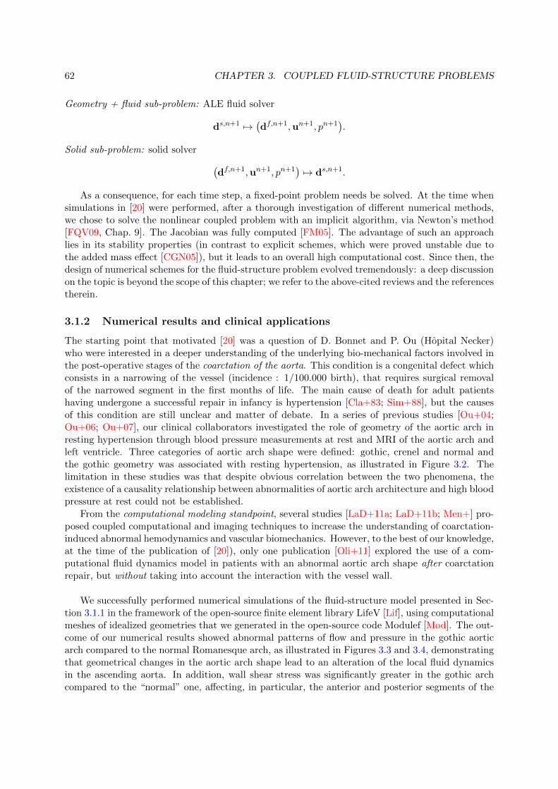
62 CHAPTER 3. COUPLED FLUID-STRUCTURE PROBLEMS
Geometry + fluid sub-problem: ALE fluid solver
ds,n+1 �→�df,n+1,un+1, pn+1
�.
Solid sub-problem: solid solver
�df,n+1,un+1, pn+1
��→ ds,n+1.
As a consequence, for each time step, a fixed-point problem needs be solved. At the time whensimulations in [20] were performed, after a thorough investigation of different numerical methods,we chose to solve the nonlinear coupled problem with an implicit algorithm, via Newton’s method[FQV09, Chap. 9]. The Jacobian was fully computed [FM05]. The advantage of such an approachlies in its stability properties (in contrast to explicit schemes, which were proved unstable due tothe added mass effect [CGN05]), but it leads to an overall high computational cost. Since then, thedesign of numerical schemes for the fluid-structure problem evolved tremendously: a deep discussionon the topic is beyond the scope of this chapter; we refer to the above-cited reviews and the referencestherein.
3.1.2 Numerical results and clinical applications
The starting point that motivated [20] was a question of D. Bonnet and P. Ou (Hopital Necker)who were interested in a deeper understanding of the underlying bio-mechanical factors involved inthe post-operative stages of the coarctation of the aorta. This condition is a congenital defect whichconsists in a narrowing of the vessel (incidence : 1/100.000 birth), that requires surgical removalof the narrowed segment in the first months of life. The main cause of death for adult patientshaving undergone a successful repair in infancy is hypertension [Cla+83; Sim+88], but the causesof this condition are still unclear and matter of debate. In a series of previous studies [Ou+04;Ou+06; Ou+07], our clinical collaborators investigated the role of geometry of the aortic arch inresting hypertension through blood pressure measurements at rest and MRI of the aortic arch andleft ventricle. Three categories of aortic arch shape were defined: gothic, crenel and normal andthe gothic geometry was associated with resting hypertension, as illustrated in Figure 3.2. Thelimitation in these studies was that despite obvious correlation between the two phenomena, theexistence of a causality relationship between abnormalities of aortic arch architecture and high bloodpressure at rest could not be established.
From the computational modeling standpoint, several studies [LaD+11a; LaD+11b; Men+] pro-posed coupled computational and imaging techniques to increase the understanding of coarctation-induced abnormal hemodynamics and vascular biomechanics. However, to the best of our knowledge,at the time of the publication of [20]), only one publication [Oli+11] explored the use of a com-putational fluid dynamics model in patients with an abnormal aortic arch shape after coarctationrepair, but without taking into account the interaction with the vessel wall.
We successfully performed numerical simulations of the fluid-structure model presented in Sec-tion 3.1.1 in the framework of the open-source finite element library LifeV [Lif], using computationalmeshes of idealized geometries that we generated in the open-source code Modulef [Mod]. The out-come of our numerical results showed abnormal patterns of flow and pressure in the gothic aorticarch compared to the normal Romanesque arch, as illustrated in Figures 3.3 and 3.4, demonstratingthat geometrical changes in the aortic arch shape lead to an alteration of the local fluid dynamicsin the ascending aorta. In addition, wall shear stress was significantly greater in the gothic archcompared to the “normal” one, affecting, in particular, the anterior and posterior segments of the
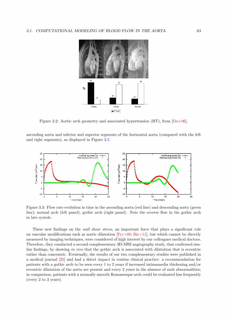
3.1. COMPUTATIONAL MODELING OF BLOOD FLOW IN THE AORTA 63
Figure 3.2: Aortic arch geometry and associated hypertension (HT), from [Ou+06].
ascending aorta and inferior and superior segments of the horizontal aorta (compared with the leftand right segments), as displayed in Figure 3.5.
Figure 3.3: Flow rate evolution in time in the ascending aorta (red line) and descending aorta (greenline); normal arch (left panel), gothic arch (right panel). Note the reverse flow in the gothic archin late systole.
These new findings on the wall shear stress, an important force that plays a significant roleon vascular modifications such as aortic dilatation [Fry+08; Bie+11], but which cannot be directlymeasured by imaging techniques, were considered of high interest by our colleagues medical doctors.Therefore, they conducted a second complementary 3D-MRI angiography study, that confirmed sim-ilar findings, by showing in vivo that the gothic arch is associated with dilatation that is eccentricrather than concentric. Eventually, the results of our two complementary studies were published ina medical journal [20] and had a direct impact in routine clinical practice: a recommendation forpatients with a gothic arch to be seen every 1 to 2 years if increased intimamedia thickening and/oreccentric dilatation of the aorta are present and every 2 years in the absence of such abnormalities;in comparison, patients with a normally smooth Romanesque arch could be evaluated less frequently(every 2 to 3 years).
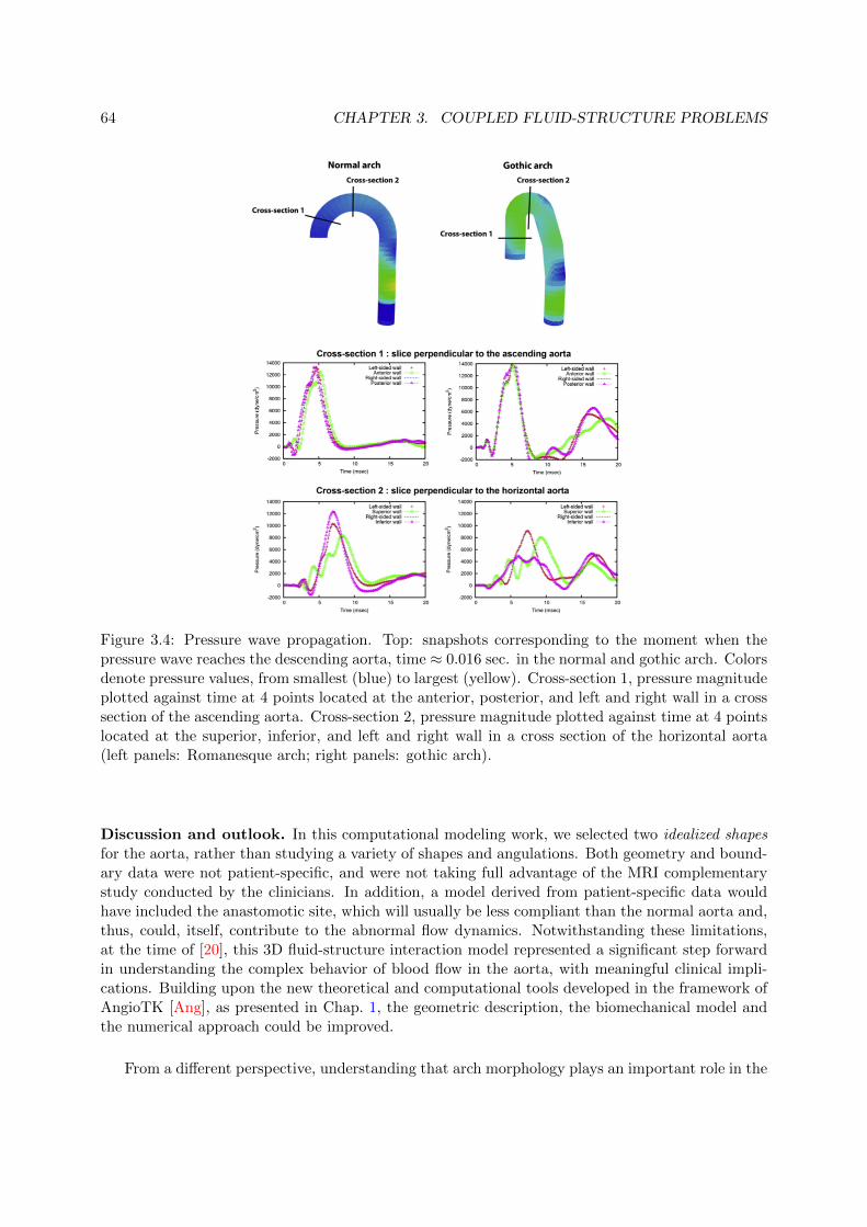
64 CHAPTER 3. COUPLED FLUID-STRUCTURE PROBLEMS
Figure 3.4: Pressure wave propagation. Top: snapshots corresponding to the moment when thepressure wave reaches the descending aorta, time ≈ 0.016 sec. in the normal and gothic arch. Colorsdenote pressure values, from smallest (blue) to largest (yellow). Cross-section 1, pressure magnitudeplotted against time at 4 points located at the anterior, posterior, and left and right wall in a crosssection of the ascending aorta. Cross-section 2, pressure magnitude plotted against time at 4 pointslocated at the superior, inferior, and left and right wall in a cross section of the horizontal aorta(left panels: Romanesque arch; right panels: gothic arch).
Discussion and outlook. In this computational modeling work, we selected two idealized shapesfor the aorta, rather than studying a variety of shapes and angulations. Both geometry and bound-ary data were not patient-specific, and were not taking full advantage of the MRI complementarystudy conducted by the clinicians. In addition, a model derived from patient-specific data wouldhave included the anastomotic site, which will usually be less compliant than the normal aorta and,thus, could, itself, contribute to the abnormal flow dynamics. Notwithstanding these limitations,at the time of [20], this 3D fluid-structure interaction model represented a significant step forwardin understanding the complex behavior of blood flow in the aorta, with meaningful clinical impli-cations. Building upon the new theoretical and computational tools developed in the framework ofAngioTK [Ang], as presented in Chap. 1, the geometric description, the biomechanical model andthe numerical approach could be improved.
From a different perspective, understanding that arch morphology plays an important role in the

3.1. COMPUTATIONAL MODELING OF BLOOD FLOW IN THE AORTA 65
Figure 3.5: Wall shear stress (WSS) mapping and magnitude. Top: WSS distribution at an instantcorresponding to the passage of the pressure wave (time ≈ 0.007 second). Colors denote WSSvalues, from smallest (blue) to largest (red). Cross-section 1, magnitude of the WSS plotted againsttime at 4 points located at the anterior, posterior, and left and right wall in a cross section of theascending aorta. Cross section 2, magnitude of the WSS plotted against time at 4 points located atthe superior, inferior, and left and right wall in a cross section of the horizontal aorta (left panels:Romanesque arch; right panels: gothic arch).
alteration of the local fluid dynamics lead us to the question of a possible interpretation of the prob-lem in terms of shape optimization. Several works reviewed in [Mar14] have already demonstratedthe potential of coupling a shape optimization approach to cardiovascular blood flow simulationswith the aim of improving surgical design. In current discussions with Y. Privat (Univ. Paris 6) andhis PhD student F. Omnes, we are exploring the possibility of numerically searching the optimalshape of the aorta by minimizing the dissipated viscous energy of the fluid, based on a theoreticaland computational framework recently developed in [Dap+17]. This research direction will hope-fully benefit from the advances of the research project Analysis and simulation of optimal shapes –application to life sciences, supported by the Paris City Hall (PI: Yannick Privat, dec. 2016–dec.2020), in which I’m involved as an associated collaborator.

66 CHAPTER 3. COUPLED FLUID-STRUCTURE PROBLEMS
3.2 Discretization in time in simulations of particulate flows
Models and simulations of the coupled dynamics of rigid or deformable bodies evolving in a sur-rounding fluid are of interest in several biological applications, as for instance understanding themicrocirculation of blood [Rah+10] or swimming bacteria [DMM11]. Among different approachesproposed in the literature, we focus in Section 3.2.1 on a microscopic model, describing the dynamicsof rigid particles in a Stokes flow. Our methodological contribution [9] tackles the issue of handlingcontacts (either between two particles or between a particle and a wall), which is a key ingredientin the direct numerical simulation of particulate flows, especially in the dense regime.
3.2.1 Dense fluid-particle flows and difficulties arising in their simulations
One of the challenges for fluid/particle flow simulations is to provide an accurate resolution of theso-called lubrication regime, when the distance between two particles immersed in the fluid or be-tween a particle and the wall becomes very small. The presence of extremely high gradients of thevelocity in the narrow gap between the particle and the wall (or between the two particles) resultsin very strong drag forces (which can be referred to as lubrication forces in this case) and thusrequires special attention in order to construct efficient and accurate discretization methods.
We consider in the sequel the case of one rigid particle immersed in a viscous, incompressiblefluid with a particular emphasis on situations when the particle approaches a plane. Despite itsapparent simplicity, this situation encompasses the main difficulties of the lubrication regime andmotivated the work in [9]. The fluid (with the particle inside) fills a fixed domain Ω⊂Rd withd = 2 or 3, and the region occupied by the particle Bt ⊂ Ω varies with time t, see Figure 3.6.Assuming that the inertial effects are negligible in the fluid and the no-slip conditions are valid onthe boundaries of Ω and Bt, the fluid motion is governed by the Stokes equations:
Figure 3.6: Geometrical setting and notations.
−νΔu+∇p = ρfg, in Ω \ Bt
∇ · u = 0, in Ω \ Bt
u = 0, on ∂Ω
u = V + ω × r on ∂Bt
(3.10)
where u and p are the velocity and the pressure in the fluid, ν and ρf are the viscosity and thedensity of the fluid, g is the external force, V = V(t) and ω = ω(t) are the translational and

3.2. DISCRETIZATION IN TIME IN SIMULATIONS OF PARTICULATE FLOWS 67
angular velocities of the rigid body Bt, r = x − G is the vector pointing from the center of massof the particle G to a point x on its boundary. The more realistic Navier-Stokes equations may beaccommodated into the framework (3.10) by including the convective term u ·∇u into g.
The fluid exerts a net force F and a torque T on the particle given by
F = F(Bt,V,ω) =
�
∂Bt
(2νD(u)− pI)ndσ, (3.11)
T = T(Bt,V,ω) =
�
∂Bt
r× (2νD(u)− pI)ndσ,
where D(u) stands for the symmetric gradient of u and n is the unit normal vector on ∂Bt directedtowards the fluid domain. Using these notations we write out the equations of motion of the particleas follows �
mdVdt = F(Bt,V,ω) +mg,
It dωdt + ω × Itω = T(Bt,V,ω),(3.12)
where m is the mass of the particle and It is its inertia tensor, expressed in the fixed Cartesianframe and thus dependent on time. Equations (3.12) are coupled with the equations describing thepropagation of the particle: �
G = V,
ri = ω × ri, i = 1, . . . , d.(3.13)
The force F is a sum of the Archimedes force due to gravity and of the drag force which is purelyhydrodynamic, i.e. obtained from (3.10) by setting g = 0. The particularity of the drag is thatit tends very rapidly to infinity when the particle approaches the wall, thus preventing collisionsbetween them. Indeed, it has been proved in [Hil07] (2D case), [HT09] (3D case) that a smoothrigid body embedded in a viscous fluid cannot touch the wall in finite time. For an overview ofexistence and uniqueness results for the coupled fluid-structure interaction problem described byEquations (3.10–3.13), including the (near-)contact regime, see [Hil14].
In the regime of very small distance between the particle and the wall, the lubrication forceis very difficult to take into account in a numerical simulation [Lef09]. The corrections specific tothe lubrication regime were proposed in the context of the boundary integral methods [QPTF00;Mam06], in that of the Stokesian Dynamics [BB88; SB01], and in that of the force-coupling method[DM03]. Short-range repulsion forces mimicking the lubrication ones were also used in [Glo+99]in the context of fictitious domain finite element methods. However, the influence of these (notnecessarily realistic) forces on the accuracy of a simulation is not well understood. Another simpleidea is just to stop the particle when it tries to penetrate the wall during a numerical simulation,but it is then not necessarily clear which criterion should be chosen to decide if the particle shouldeventually bounce off the wall and when it should it happen. These questions have a partial answerin the articles [Mau07; Lef09] on the gluey particle model. It is shown there that the particletrajectory satisfies an integro-differential equation in the limit of vanishing viscosity, which is easyto discretize in time using moderate time steps and which predicts the moment of an eventualrebound from the wall. We pursued a similar idea in our approach described in the next section,but our aim is to construct an approximated trajectory of the particle in the lubrication regimethat would be accurate enough for any given value of the viscosity, not necessarily small.
3.2.2 A model ordinary differential equation with lubrication forces
Formulation of the problem and construction of an approximated solution. To describe

68 CHAPTER 3. COUPLED FLUID-STRUCTURE PROBLEMS
our strategy, we consider the following simplified setting: Ω ⊂ R2 is the half-plane {(x, y), y > 0}and the particle is a disk of radius R. Let moreover g(t) = g(t)e2 and assume the particle isat rest at the initial time. The x-component of the particle velocity and its angular velocity willthen vanish at all time. The position of the particle is fully determined by its distance q from thebottom, as in Figure 3.6. The net force F is the sum of the drag, which is a function of q and V,linear in V, and of the Archimedes force:
F = −n(q)V +mag(t)e2, with ma = m− ρf |Bt|,
where n(q) is the drag coefficient computed by the Stokes equations (3.10). Denoting the y-component of the velocity by v, we are thus led to the following differential equations
�mv = −n(q)v +mag,
q = v.(3.14)
In [9] we provide the following derivation of the asymptotic expansion for the lubrication force actingon a disk immersed in a Newtonian fluid and approaching the wall:
Theorem 3.2.1. The viscous drag force satisfies F = −n(q)V where
n(q) = 3√2πν
�R
q
� 32
[1 + ε(q)] ,
with ε(q) → 0 when q → 0.
The proof of Theorem 3.2.1 is divided into three steps. First, we use the variational formulationfor the solution (u, p) to (3.10) to compute the associated drag coefficient n(q) in the expression forviscous drag F = −n(q)V. Second, we deduce from the variational formulation the lower and upperbounds for n(q). We conclude the proof by computing an asymptotic expansion of the bounds ofthis range.
Remark 3.2.2. The equivalent result in the three-dimensional setting is well-known but to thebest of our knowledge it was new in two dimensions. The proof method also extends to the three-dimensional setting with small changes and can be adapted to other boundary conditions.
After eliminating v from the system (3.14) and going to non-dimensional variables, we obtainthe following equation for q(t):
q = −n(q)q + g, (3.15)
where n(q) = ε/q32 in the two-dimensional case, n(q) = ε/q in the three-dimensional case, respec-
tively and ε depends on the characteristic values of g, of the fluid and the solid. We remind thatequations of the type (3.15) are at the basis of the gluey particle model of [Mau07; Lef09], thatconsists in considering the limit ε → 0, which is physically the limit of vanishing viscosity. Notehowever that in practice ε computed from the non-dimensionalization procedure is not necessarilysmall.
In the lubrication regime of q → 0, the drag coefficient n(q) tends to infinity, which can createdifficulties when computing numerical solutions of (3.15). In order to overcome this problem,one should either use a very small time step when discretizing the equation, but this can becomecomputationally expensive, or propose a strategy to prevent q from becoming too small. Theapproach we proposed in [9], inspired by the latter idea, consists in introducing a threshold valueqs for the distance q, below which, instead of solving (3.15), we introduce an alternative model andconstruct a sufficiently accurate “approximate” solution q instead of the “true” solution q. Theconstruction of the approximated trajectory is the following:

3.2. DISCRETIZATION IN TIME IN SIMULATIONS OF PARTICULATE FLOWS 69
• we first assume that q(t) is the same as q(t) until the latter hits qs for the first time at t = t1;
• next, the trajectory q(t) is frozen until the time t = t2, which is the first instant after t1 whenv(t) = 0, where
v(t) = q(t1) +
� t
t1
g(s)ds. (3.16)
• afterwards, the trajectory resumes again as a solution to (3.15) starting from qs with zerovelocity:
q(t) =
q(t), for 0 < t < t1qs, for t1 ≤ t < t2solution to (3.15) with q(t2) = qs, q(t2) = 0, for t ≥ t2
(3.17)
In the in the special case when g(t) is given by
g(t) =
�g−(t) < 0, for t ≤ t0,
g+ > 0, for t > t0,(3.18)
with some positive constants t0, g+ and a negative function g−(t), with the above notations, weprove the following result:
Proposition 3.2.1. If g(t) is given by (3.18), then
0 ≤ t2 − t2 ≤1
n(qs),
supt∈[0,t2]
|q(t)− q(t)| ≤ qs, (3.19)
|q(t2)− ˙q(t2)| = q(t2) ≤g+
n(qs).
Remark 3.2.3. Proposition 3.2.1 should be interpreted as an estimate of the approximation errorand also as a guideline on how to choose the threshold value qs, depending on g and the time step insuch a way that the quantity g+
n(qs)has the same order of magnitude as the precision in the numerical
scheme. Since n(q) → 0 when q → 0, the smaller the threshold, the smaller the error. However,taking qs too small may deteriorate the accuracy of the solution (indeed, the original goal of theintroduction of qs was to avoid the extremely small values of q). On the other hand, taking qs toolarge may unnecessarily perturb the solution in the regions where a straightforward discretizationcould give more precise results.
Numerical strategy and results. We analyzed the performances of three different algorithmsto solve (3.15). Algorithm 1 consists in a straightforward Euler discretization in time of (3.15),but it does not always work in the near-contact regime, since it does not necessarily provide apositive approximation qk. To tackle this issue, we propose in Algorithm 2 the construction of theapproximated trajectory q, with an a priori chosen threshold value qs > 0, Finally, we combine inAlgorithm 3 an adaptative strategy for the choice of the time step with the threshold approximationgiven by Algorithm 2.
As an illustration, we show in Fig. 3.7 a comparison between Algorithm 1, unable to produce aphysically acceptable solution even with very small Δt = 0.0001 and Algorithm 2, which providessatisfactory results, in a two-dimensional setting for ε = 10−3. In order to better observe the quasi-contact region and the effect of introducing the threshold in Algorithm 2, we zoom on small distances

70 CHAPTER 3. COUPLED FLUID-STRUCTURE PROBLEMS
by passing to a log-scale in Figure 3.8 (left panel). The results are compared with computationsusing Algorithm 3 with adapted stepsize and taking a number of values for Δtmin (right panel). Wegive in particular the results with Δtmin = 0, so that Algorithm 3 is reduced to a standard timemarching scheme with automatically adapted step sizes. In practice, we noticed that step sizes Δtof the order 10−4 were actually sufficient to satisfy our error tolerance criterion almost everywhereapart from a very small range of time around 1, where Algorithm 3 chooses Δt of the order 10−8.Setting Δtmin to 10−3 or 10−4 avoids such small time steps and gives fairly good results.
t
q
0 2 4
-6
-5
-4
-3
-2
-1
0
1
exact
0.1
0.01
0.001
0.0001
t
q
0 2 4
0
0.2
0.4
0.6
0.8
1
1.2
exact
0.1
0.01
0.001
0.0001
Figure 3.7: Solution to the ODE (3.15) with n(q) = ε/q3/2, ε = 10−3. Left: the exact solution andsolutions obtained by Algorithm 1 with Δt ranging from 0.1 to 0.0001. Right: solutions obtainedby Algorithm 2 with Δt in the same range. The results obtained with Δt ≤ 0.01 on the right arevisually indistinguishable from the exact solution.
t
q
0 2 4
10-6
10-5
10-4
10-3
10-2
10-1
100
exact
0.1
0.01
0.001
0.0001
t
q
0 2 4
10-6
10-5
10-4
10-3
10-2
10-1
100
exact
0
0.001
0.0001
Figure 3.8: Solution to the ODE (3.15) with n(q) = ε/q3/2, ε = 10−3 (log scale). Left: solution ob-tained by Algorithm 2, choosing qs so that n(qs) = 1/(20Δt). Right: results obtained by Algorithm3 with tol = 10−5 and different values of Δtmin specified in the legend.
Towards more complex configurations. Although developments in [9] are only for the modelequation (3.15), we have in mind a possible incorporation of our time marching schemes into a fullsimulation of flow with solid particles. The coefficient n(q) will be then given by a solution to theStokes system at each time step where q represents the surface-wall distance in the case of a particleapproaching to the wall or the inter-particle distance in the case of two approaching particles. The“external” force g(t) in (3.15) will then include the components of the physical external forces, like

3.3. CONCLUSIONS AND OUTLOOK 71
gravitational force, in the direction connecting the closest points on the surfaces of nearly touchingparticles, plus other corrections. Most importantly, these include the part of hydrodynamic dragdue to the convective terms in the Navier-Stokes system, if the convective terms in the fluid motionequation are not neglected. The time marching scheme should thus work robustly for any righthand side g(t), in particular for a function changing the sign. Indeed, a possible scenario even inthe simplest test case of a particle falling under its weight on a horizontal wall (so that g(t) isnegative in the beginning) could be that the convective terms in Navier-Stokes equations becomeso important at some point in time that they prevail over the gravitation force and g(t) becomespositive, which may lead to the rebound of the particle. The next step could take into account thecase of deformable bodies evolving in a fluid flow.
Another perspective of the present approach is to include more complex solid movements. Inthis direction, it would be interesting to carry out simulations in the following configurations: (i)kissing phase in the ”Drafting-Kissing-Tumbling” [FJL87]: the fall of a homogeneous disk under theaction of the gravity force in a cavity which contains a hole in form of a disk; (ii) the sedimentationof a particle which is almost in contact with a vertical wall [Cox74]. In both cases the problemwould be solved in the lubrication approximation.
3.3 Conclusions and outlook
We summarized in this chapter two contributions where biomedical questions were treated from themathematical and computational viewpoint as coupled fluid-structure interaction problems. Basedon a careful description of the bio-mechanical phenomena into play, we addressed these questionsby means of efficient numerical methods, either selected within the state-of-the-art context or newlydeveloped for the specific problem in view. In the previous chapters, we focused on the fluid mechan-ical aspects of the problems, governed by the Navier-Stokes equations or by reduced fluid models,possibly coupled in a geometrical multiscale framework. Here the complexity and the challengescame from the multiphysics approach, in which the fluid equations are coupled with a system ofequations describing the dynamics of a rigid or deformable solid.
Chronologically, these were the first works I developed in mathematical biology and numerousperspectives are now possible due to recent developments in the field. Besides the extensions al-ready mentioned at the end of each section, a last comment, taking as a starting point the examplestreated in this chapter. On one hand, the two problems share a similar mathematical structureand therefore a unified language was utilized to solve them, with new analytical and numericalmethods. On the other hand, the first one involves a complex three-dimensional, highly nonlinearfluid-structure model, with the goal of answering a medical question, whereas the second one is a toymodel that brings a methodological answer to a simplified, yet meaningful biological problem. Thetwo of them are illustrative and somehow dual aspects in the interplay between what we know andwhat we want to solve, both in mathematics and in biology or medicine, with infinite possibilitiesof cross-fertilization of ideas. In this spirit, the conclusion of the chapter, and more generally of themanuscript, is the following call for new challenges and opportunities:
Mathematics is biology’s next microscope, only better;biology is mathematics’ next physics, only better.
Joel Cohen (Rockefeller and Columbia Universities, NY, 2004).

72 CHAPTER 3. COUPLED FLUID-STRUCTURE PROBLEMS
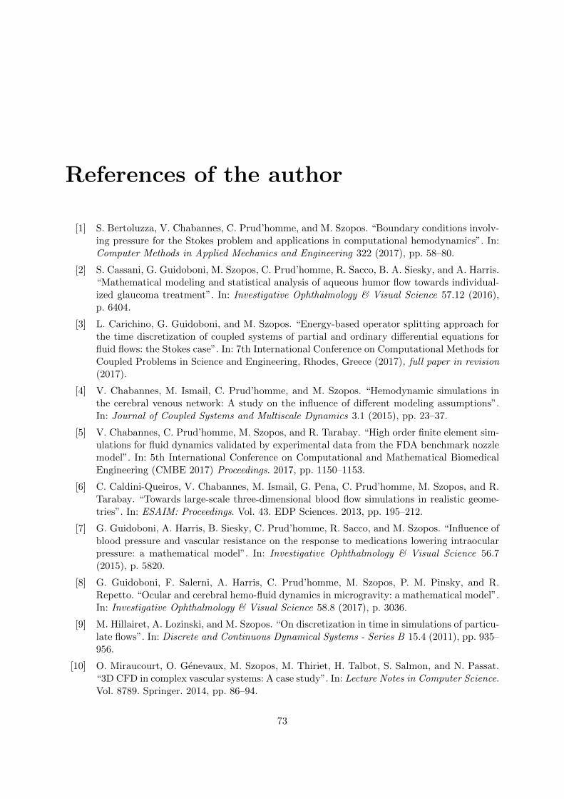
References of the author
[1] S. Bertoluzza, V. Chabannes, C. Prud’homme, and M. Szopos. “Boundary conditions involv-ing pressure for the Stokes problem and applications in computational hemodynamics”. In:Computer Methods in Applied Mechanics and Engineering 322 (2017), pp. 58–80.
[2] S. Cassani, G. Guidoboni, M. Szopos, C. Prud’homme, R. Sacco, B. A. Siesky, and A. Harris.“Mathematical modeling and statistical analysis of aqueous humor flow towards individual-ized glaucoma treatment”. In: Investigative Ophthalmology & Visual Science 57.12 (2016),p. 6404.
[3] L. Carichino, G. Guidoboni, and M. Szopos. “Energy-based operator splitting approach forthe time discretization of coupled systems of partial and ordinary differential equations forfluid flows: the Stokes case”. In: 7th International Conference on Computational Methods forCoupled Problems in Science and Engineering, Rhodes, Greece (2017), full paper in revision(2017).
[4] V. Chabannes, M. Ismail, C. Prud’homme, and M. Szopos. “Hemodynamic simulations inthe cerebral venous network: A study on the influence of different modeling assumptions”.In: Journal of Coupled Systems and Multiscale Dynamics 3.1 (2015), pp. 23–37.
[5] V. Chabannes, C. Prud’homme, M. Szopos, and R. Tarabay. “High order finite element sim-ulations for fluid dynamics validated by experimental data from the FDA benchmark nozzlemodel”. In: 5th International Conference on Computational and Mathematical BiomedicalEngineering (CMBE 2017) Proceedings. 2017, pp. 1150–1153.
[6] C. Caldini-Queiros, V. Chabannes, M. Ismail, G. Pena, C. Prud’homme, M. Szopos, and R.Tarabay. “Towards large-scale three-dimensional blood flow simulations in realistic geome-tries”. In: ESAIM: Proceedings. Vol. 43. EDP Sciences. 2013, pp. 195–212.
[7] G. Guidoboni, A. Harris, B. Siesky, C. Prud’homme, R. Sacco, and M. Szopos. “Influence ofblood pressure and vascular resistance on the response to medications lowering intraocularpressure: a mathematical model”. In: Investigative Ophthalmology & Visual Science 56.7(2015), p. 5820.
[8] G. Guidoboni, F. Salerni, A. Harris, C. Prud’homme, M. Szopos, P. M. Pinsky, and R.Repetto. “Ocular and cerebral hemo-fluid dynamics in microgravity: a mathematical model”.In: Investigative Ophthalmology & Visual Science 58.8 (2017), p. 3036.
[9] M. Hillairet, A. Lozinski, and M. Szopos. “On discretization in time in simulations of particu-late flows”. In: Discrete and Continuous Dynamical Systems - Series B 15.4 (2011), pp. 935–956.
[10] O. Miraucourt, O. Genevaux, M. Szopos, M. Thiriet, H. Talbot, S. Salmon, and N. Passat.“3D CFD in complex vascular systems: A case study”. In: Lecture Notes in Computer Science.Vol. 8789. Springer. 2014, pp. 86–94.
73

74 REFERENCES OF THE AUTHOR
[11] O. Miraucourt, S. Salmon, M. Szopos, and M. Thiriet. “Blood flow in the cerebral venoussystem: modeling and simulation”. In: Computer methods in biomechanics and biomedicalengineering 20.5 (2017), pp. 471–482.
[12] S. Mardare and M. Szopos. “Linear and nonlinear Korn inequalities on curves in R3”. In:Analysis and Applications 3.03 (2005), pp. 251–270.
[13] N. Passat, S. Salmon, J.-P. Armspach, B. Naegel, C. Prud’homme, H. Talbot, A. Fortin, S.Garnotel, O. Merveille, O. Miraucourt, R. Tarabay, V. Chabannes, A. Dufour, A. Jezierska,O. Baledent, E. Durand, L. Najman, M. Szopos, A. Ancel, J. Baruthio, M. Delbany, S. Fall,G. Page, O. Genevaux, M. Ismail, P. Loureiro de Sousa, M. Thiriet, and J. Jomier. “FromReal MRA to Virtual MRA: Towards an Open-Source Framework”. In: Lecture Notes inComputer Science, International Conference on Medical Image Computing and ComputerAssisted Intervention (MICCAI 2016). Vol. 9902. Springer, 2016, pp. 335–343.
[14] R. Sacco, S. Cassani, G. Guidoboni, M. Szopos, C. Prud’homme, and A. Harris. “Mod-eling the coupled dynamics of ocular blood flow and production and drainage of aqueoushumor”. In: 4th International Conference on Computational and Mathematical BiomedicalEngineering (CMBE 2015) Proceedings. 2015, pp. 608–611.
[15] L. Sala, C. Prud’homme, D. Prada, F. Salerni, C. Trophime, V. Chabannes, M. Szopos,R. Repetto, S. Bertoluzza, R. Sacco, A. Harris, and G. Guidoboni. “Patient-specific virtualsimulator of tissue perfusion in the lamina cribrosa”. In: Investigative Ophthalmology &Visual Science 58.8 (2017), p. 727.
[16] L. Sala, C. Prud’homme, M. Szopos, and G. Guidoboni. “Towards a full model for ocularbiomechanics, fluid dynamics and hemodynamics”. In: J. for Modeling in OphthalmologyESB–ITA 2017 extended abstract, to appear (2017).
[17] F. Salerni, R. Repetto, A. Harris, P. Pinsky, C. Prud’homme, M. Szopos, and G. Guidoboni.“Mathematical modelling of ocular and cerebral hemo-fluid dynamics: application to VIIP”.In: J. for Modeling in Ophthalmology ESB–ITA 2017 extended abstract, to appear, full paperin preparation. (2017).
[18] S. Salmon, S. Sy, and M. Szopos. “Cerebral blood flow simulations in realistic geometries”.In: ESAIM: Proceedings. Vol. 35. EDP Sciences. 2012, pp. 281–286.
[19] F. Stefanoni, A. Harris, M. Szopos, C. Prud’homme, R. Sacco, D. Messenio, M. L. Costantino,and G. Guidoboni. “Clinical assessment of intraocular pressure: a whole eye dynamic model”.In: J. for Modeling in Ophthalmology ESB–ITA 2017 extended abstract, to appear (2017).
[20] M. Szopos, N. Poussineau, Y. Maday, C. Canniffe, D. Celermajer, D. Bonnet, and P. Ou.“Computational modeling of blood flow in the aortainsights into eccentric dilatation of theascending aorta after surgery for coarctation”. In: The Journal of thoracic and cardiovascularsurgery 148.4 (2014), pp. 1572–1582.
[21] M. Szopos, S. Cassani, G. Guidoboni, C. Prud’homme, R. Sacco, B. Siesky, and A. Harris.“Mathematical modeling of aqueous humor flow and intraocular pressure under uncertainty:towards individualized glaucoma management”. In: J. for Modeling in Ophthalmology 1.2(2016), pp. 29–39.
[22] M. Szopos. “On the recovery and continuity of a submanifold with boundary in higherdimensions”. In: Comptes Rendus Mathematique 339.4 (2004), pp. 265–270.
[23] M. Szopos. “On the recovery of a curve isometrically immersed in En”. In: Chinese Annalsof Mathematics 25.04 (2004), pp. 507–522.

REFERENCES OF THE AUTHOR 75
[24] M. Szopos. “Sur la reconstruction d’une courbe isometriquement immergee dans un espaceEuclidien”. In: Comptes rendus-Mathematique 6.338 (2004), pp. 447–452.
[25] M. Szopos. “On the recovery and continuity of a submanifold with boundary”. In: Analysisand Applications 3.02 (2005), pp. 119–143.
[26] M. Szopos. “An existence and uniqueness result for isometric immersions with little regular-ity”. In: Rev. Roumaine. Math. Pures Appl 53 (2008), pp. 555–565.

76 REFERENCES OF THE AUTHOR

Other references
[AGL16] M. Aletti, J.-F. Gerbeau, and D. Lombardi. “Modeling autoregulation in three-dimensionalsimulations of retinal hemodynamics”. In: Journal for Modeling in Ophthalmology 1.1(2016), pp. 88–115.
[Ale17] M. Aletti. “Mathematical Modelling and Simulations of the Hemodynamics in theeye”. Theses. Universite Pierre et Marie Curie (UPMC Paris 6), May 2017.
[Anc+16] A. Ancel, A. Fortin, S. Garnotel, O. Miraucourt, and R. Tarabay. “PHANTOM project:development and validation of the pipeline from MRA acquisition to MRA simula-tions”. In: ESAIM: Proceedings and Surveys 55 (2016), pp. 1–22.
[Ang] AngioTK: An Open Platform to reconstruct vessels from MRI images and simulateflows to ultimately provide Virtual Angiographies. https://github.com/vivabrain/angiotk. Accessed: 2017-08-09.
[Bal+16] S. Balay, S. Abhyankar, M. F. Adams, J. Brown, P. Brune, K. Buschelman, L. Dalcin,V. Eijkhout, W. D. Gropp, D. Kaushik, M. G. Knepley, L. Curfman McInnes, K. Rupp,B. F. Smith, S. Zampini, H. Zhang, and H. Zhang. PETSc Users Manual. Tech. rep.ANL-95/11 - Revision 3.7. Argonne National Laboratory, 2016.
[Bau+16] M. Baudin, A. Dutfoy, B. Iooss, and A.-L. Popelin. “OpenTURNS: An IndustrialSoftware for Uncertainty Quantification in Simulation”. In: Handbook of UncertaintyQuantification. Cham: Springer International Publishing, 2016, pp. 1–38.
[BB88] J. F. Brady and G. Bossis. “Stokesian dynamics”. In: Annual review of fluid mechanics20.1 (1988), pp. 111–157.
[BCRY15] C. Bernardi, T. Chacon Rebollo, and D. Yakoubi. “Finite Element Discretization ofthe Stokes and Navier-Stokes Equations with Boundary Conditions on the Pressure”.In: SIAM Journal on Numerical Analysis 53.3 (2015), pp. 1256–1279.
[BF12] F. Brezzi and M. Fortin. Mixed and hybrid finite element methods. Vol. 15. SpringerScience & Business Media, 2012.
[BGM10] L. Baffico, C. Grandmont, and B. Maury. “Multiscale modeling of the respiratorytract”. In: Mathematical Models and Methods in Applied Sciences 20.01 (2010), pp. 59–93.
[BGN14] T. Bodnar, G. P. Galdi, and S. Necasova. Fluid-Structure Interaction and BiomedicalApplications. Springer, 2014.
[BHM16] W. Bradley, V. Haughton, and K.-A. Mardal. “Cerebrospinal fluid flow in adults”. In:Handbook of Clinical Neurology 135 (2016), pp. 591–601.
77

78 OTHER REFERENCES
[Bie+11] E. T. Bieging, A. Frydrychowicz, A. Wentland, B. R. Landgraf, K. M. Johnson, O.Wieben, and C. J. Fran¸cois. “In vivo three-dimensional MR wall shear stress estima-tion in ascending aortic dilatation”. In: Journal of Magnetic Resonance Imaging 33.3(2011), pp. 589–597.
[Bru75] R. F. Brubaker. “The effect of intraocular pressure on conventional outflow resistancein the enucleated human eye.” In: Investigative ophthalmology & visual science 14.4(1975), pp. 286–292.
[Beg+87] C. Begue, C. Conca, F. Murat, and O. Pironneau. “A nouveau sur les equations deStokes et de Navier-Stokes avec des conditions aux limites sur la pression”. In: Comptesrendus de l’Academie des sciences. Serie 1, Mathematique 304.1 (1987), pp. 23–28.
[Cai+15] A. Caiazzo, G. Montecinos, L. O. Muller, E. M. Haacke, and E. F. Toro. “Computa-tional haemodynamics in stenotic internal jugular veins”. In: Journal of mathematicalbiology 70.4 (2015), pp. 745–772.
[Cai+17] A. Caiazzo, F. Caforio, G. Montecinos, L. O. Muller, P. J. Blanco, and E. F. Toro.“Assessment of reduced-order unscented Kalman filter for parameter identification in1-dimensional blood flow models using experimental data”. In: International Journalfor Numerical Methods in Biomedical Engineering 33.8 (2017), e2843–n/a.
[Car+84] R. S. Carel, A. D. Korczyn, M. Rock, and I. Goya. “Association between ocular pres-sure and certain health parameters”. In: Ophthalmology 91.4 (1984), pp. 311–314.
[CGL09] B. Cockburn, J. Gopalakrishnan, and R. Lazarov. “Unified hybridization of discon-tinuous Galerkin, mixed, and continuous Galerkin methods for second order ellipticproblems”. In: SIAM Journal on Numerical Analysis 47.2 (2009), pp. 1319–1365.
[CGN05] P. Causin, J.-F. Gerbeau, and F. Nobile. “Added-mass effect in the design of par-titioned algorithms for fluid–structure problems”. In: Computer methods in appliedmechanics and engineering 194.42 (2005), pp. 4506–4527.
[Cla+83] P. M. Clarkson, M. R. Nicholson, B. G. Barratt-Boyes, J. M. Neutze, and R. M.Whitlock. “Results after repair of coarctation of the aorta beyond infancy: a 10 to28 year follow-up with particular reference to late systemic hypertension”. In: TheAmerican journal of cardiology 51.9 (1983), pp. 1481–1488.
[CMP94] C. Conca, F. Murat, and O. Pironneau. “The Stokes and Navier-Stokes equations withboundary conditions involving the pressure”. In: Japanese journal of mathematics. Newseries 20.2 (1994), pp. 279–318.
[Coc+97] C. A. Cocosco, V. Kollokian, R. K.-S. Kwan, G. B. Pike, and A. C. Evans. “Brainweb:Online interface to a 3D MRI simulated brain database”. In: NeuroImage. Citeseer.1997, S425.
[Con+95] C. Conca, C. Pares, O. Pironneau, and M. Thiriet. “Navier-Stokes equations withimposed pressure and velocity fluxes”. In: International journal for numerical methodsin fluids 20.4 (1995), pp. 267–287.
[Cox74] R. G. Cox. “The motion of suspended particles almost in contact”. In: InternationalJournal of Multiphase Flow 1.2 (1974), pp. 343–371.
[Dap+17] C. Dapogny, P. Frey, F. Omnes, and Y. Privat. “Geometrical shape optimizationin fluid mechanics using Freefem++”. Preprint, https://hal.archives-ouvertes.fr/hal-01481707/. 2017.

OTHER REFERENCES 79
[DM03] S. L. Dance and M. R. Maxey. “Incorporation of lubrication effects into the force-coupling method for particulate two-phase flow”. In: Journal of Computational Physics189.1 (2003), pp. 212 –238.
[DMM11] A. Decoene, S. Martin, and B. Maury. “Microscopic modelling of active bacterialsuspensions”. In: Mathematical Modelling of Natural Phenomena 6.5 (2011), pp. 98–129.
[DQ08] C. D’Angelo and A. Quarteroni. “On the coupling of 1D and 3D diffusion-reactionequations: applications to tissue perfusion problems”. In: Mathematical Models andMethods in Applied Sciences 18.08 (2008), pp. 1481–1504.
[EM15] Ø. Evju and K.-A. Mardal. “On the assumption of laminar flow in physiological flows:Cerebral aneurysms as an illustrative example”. In: Modeling the Heart and the Cir-culatory System. Springer, 2015, pp. 177–195.
[ESW14] H. C. Elman, D. J. Silvester, and A. J. Wathen. Finite elements and fast iterativesolvers: with applications in incompressible fluid dynamics. Numerical Mathematics &Scientific Computation, 2014.
[Evj11] Ø. Evju. “Sensitivity analysis of simulated blood flow in cerebral aneurysms”. MAthesis. 2011.
[EVSM13] Ø. Evju, K. Valen-Sendstad, and K.-A. Mardal. “A study of wall shear stress in 12aneurysms with respect to different viscosity models and flow conditions”. In: Journalof biomechanics 46.16 (2013), pp. 2802–2808.
[Eyea] Eye-CSF connection. https://www.webmedcentral.com/article_view/3382. Ac-cessed: 2017-08-17.
[Eyeb] Eye2Brain arteries. http://biology.stackexchange.com/questions/9637/. Ac-cessed: 2017-08-17.
[Eyec] Eye2Brain veins. http://en.wikipedia.org/wiki/Cavernous_sinus. Accessed:2017-08-17.
[Fee] Feel++: Finite Element Embedded Library in C++. http://www.feelpp.org. Ac-cessed: 2017-07-18.
[Fen13] M. A. Fenandez. “Incremental displacement-correction schemes for incompressiblefluid-structure interaction”. In: Numer. Math. 123 (2013), pp. 21–65.
[FI14] J. Fouchet-Incaux. “Artificial boundaries and formulations for the incompressible Navier–Stokes equations: applications to air and blood flows”. In: SeMA Journal 64.1 (2014),pp. 1–40.
[Fig+06] C. A. Figueroa, I. E. Vignon-Clementel, K. E. Jansen, T. J. Hughes, and C. A. Tay-lor. “A coupled momentum method for modeling blood flow in three-dimensional de-formable arteries”. In: Computer methods in applied mechanics and engineering 195.41(2006), pp. 5685–5706.
[FIGM15] J. Fouchet-Incaux, C. Grandmont, and S. Martin. Numerical stability of couplingschemes in the 3d/0d modelling of airflows and blood flows, Retrieved from:https://hal.inria.fr/hal-01095960. 2015.
[FJL87] A. F. Fortes, D. D. Joseph, and T. S. Lundgren. “Nonlinear mechanics of fluidizationof beds of spherical particles”. In: Journal of Fluid Mechanics 177 (1987), pp. 467–483.
80 OTHER REFERENCES
[FLV15] M. A. Fenandez, M. Landajuela, and M. Vidrascu. “Fully decoupled time-marchingschemes for incompressible fluid/thin-walled structure interaction”. In: J. Comput.Phys. 297 (2015), pp. 156–181.
[FM05] M. A. Fernandez and M. Moubachir. “A Newton method using exact Jacobians forsolving fluid–structure coupling”. In: Computers & Structures 83.2 (2005), pp. 127–142.
[FQV09] L. Formaggia, A. Quarteroni, and A. Veneziani. Cardiovascular mathematics, volume1 of MS&A. Modeling, Simulation and Applications. 2009.
[Fry+08] A. Frydrychowicz, A. Berger, M. F. Russe, A. F. Stalder, A. Harloff, S. Dittrich, J.Hennig, M. Langer, and M. Markl. “Time-resolved magnetic resonance angiographyand flow-sensitive 4-dimensional magnetic resonance imaging at 3 Tesla for blood flowand wall shear stress analysis”. In: The Journal of thoracic and cardiovascular surgery136.2 (2008), pp. 400–407.
[FV12] L. Formaggia and C. Vergara. “Prescription of general defective boundary conditionsin fluid-dynamics”. In: Milan Journal of Mathematics (2012), pp. 1–18.
[Gad+15] G. Gadda, A. Taibi, F. Sisini, M. Gambaccini, P. Zamboni, and M. Ursino. “A newhemodynamic model for the study of cerebral venous outflow”. In: American Journalof Physiology-Heart and Circulatory Physiology 308.3 (2015), H217–H231.
[Gar16] S. Garnotel. “Modelisation numerique de la pression intracranienne via les ecoulementsdu sang et du liquide cerebrospinal mesures par IRM de flux.” PhD thesis. Universitede Picardie Jules Verne, 2016.
[Gid+96] P. Gideon, C. Thomsen, F. Gjerris, P. S. Sørensen, F. Stahlberg, and O. Henriksen.“Measurement of blood flow in the superior sagittal sinus in healthy volunteers, and inpatients with normal pressure hydrocephalus and idiopathic intracranial hypertensionwith phase-contrast cine MR imaging”. In: Acta Radiologica 37.1P1 (1996), pp. 171–176.
[Gir90] V. Girault. “Curl-conforming finite element methods for Navier-Stokes equations withnon-standard boundary conditions in R3”. In: The Navier-Stokes Equations Theoryand Numerical Methods. Springer, 1990, pp. 201–218.
[Gis+04] J. Gisolf, J. J. Van Lieshout, K. Van Heusden, F. Pott, W. J. Stok, and J. M. Kare-maker. “Human cerebral venous outflow pathway depends on posture and centralvenous pressure”. In: The Journal of physiology 560.1 (2004), pp. 317–327.
[Glo+99] R. Glowinski, T. W. Pan, T. I. Hesla, and D. D. Joseph. “A distributed Lagrangemultiplier/fictitious domain method for particulate flows”. In: International Journalof Multiphase Flow 25.5 (1999), pp. 755 –794.
[Glo03] R. Glowinski. Handbook of Numerical Analysis : Numerical methods for Fluids (Part3), Philippe G. Ciarlet and Jacques-Louis Lions(Eds). Vol. IX. North-Holland, 2003.
[Gui+14] G. Guidoboni, A. Harris, S. Cassani, J. Arciero, B. Siesky, A. Amireskandari, L. Tobe,P. Egan, I. Januleviciene, and J. Park. “Intraocular Pressure, Blood Pressure, and Reti-nal Blood Flow Autoregulation: A Mathematical Model to Clarify Their Relationshipand Clinical Relevance”. In: Investigative ophthalmology & visual science 55.7 (2014),pp. 4105–4118.

OTHER REFERENCES 81
[Har+11] P. Hariharan, M. Giarra, V. Reddy, S. W Day, K. B. Manning, S. Deutsch, S. F. CStewart, M. R Myers, M. R Berman, G. W. Burgreen, et al. “Multilaboratory particleimage velocimetry analysis of the FDA benchmark nozzle model to support validationof computational fluid dynamics simulations”. In: Journal of biomechanical engineering133.4 (2011), p. 041002.
[Hec12] F. Hecht. “New development in FreeFem++”. In: Journal of numerical mathematics20.3-4 (2012), pp. 251–266.
[Her+13] S. M. Heringa, W. H. Bouvy, E. van den Berg, A. C. Moll, L. J. Kappelle, and G. J.Biessels. “Associations between retinal microvascular changes and dementia, cognitivefunctioning, and brain imaging abnormalities: a systematic review”. In: J Cereb BloodFlow Metab 33.7 (2013), pp. 983–995.
[Hil07] M. Hillairet. “Lack of collision between solid bodies in a 2D incompressible viscousflow”. In: Communications in Partial Differential Equations 32.9 (2007), pp. 1345–1371.
[Hil14] M. Hillairet. “Topics in the Mathematical Theory of Interactions of IncompressibleViscous Fluid with Rigid Bodies”. In: Fluid-Structure Interaction and Biomedical Ap-plications. Ed. by T. Bodnar, G. P. Galdi, and S. Necasova. Basel: Springer Basel,2014, pp. 257–320.
[HMH13] H. Ho, K. Mithraratne, and P. Hunter. “Numerical simulation of blood flow in ananatomically-accurate cerebral venous tree”. In: IEEE transactions on medical imaging32.1 (2013), pp. 85–91.
[HRT96] J. G. Heywood, R. Rannacher, and S. Turek. “Artificial boundaries and flux andpressure conditions for the incompressible Navier-Stokes equations.” In: InternationalJournal for Numerical Methods in Fluids 22 (1996), pp. 325–352.
[HT09] M. Hillairet and T. Takahashi. “Collisions in three-dimensional fluid structure inter-action problems”. In: SIAM Journal on Mathematical Analysis 40.6 (2009), pp. 2451–2477.
[JG11] K. A. Johnson and R. S. Goody. “The original Michaelis constant: translation of the1913 Michaelis–Menten paper”. In: Biochemistry 50.39 (2011), pp. 8264–8269.
[Jin15] V. Jindal. “Interconnection Between Brain and Retinal Neurodegenerations”. In:Molec-ular neurobiology 51.3 (2015), pp. 885–892.
[Kie+11] J. W. Kiel, M. Hollingsworth, R. Rao, M. Chen, and H. A. Reitsamer. “Ciliary bloodflow and aqueous humor production”. In: Progress in retinal and eye research 30.1(2011), pp. 1–17.
[Kur11] V. Kurtcuoglu. “Biomechanics of the Brain”. In: Springer New York, 2011. Chap. 8:Computational fluid dynamics for the assessment of cerebrospinal fluid flow and itscoupling with cerebral blood flow.
[LaD+11a] J. F. LaDisa, R. J. Dholakia, C. A. Figueroa, I. E. Vignon-Clementel, F. P. Chan, M.M. Samyn, J. R. Cava, C. A. Taylor, and J. A. Feinstein. “Computational SimulationsDemonstrate Altered Wall Shear Stress in Aortic Coarctation Patients Treated byResection with End-to-end Anastomosis”. In: Congenital Heart Disease 6.5 (2011),pp. 432–443.

82 OTHER REFERENCES
[LaD+11b] J. F. LaDisa, C. A. Figueroa, I. E. Vignon-Clementel, H. J. Kim, N. Xiao, L. M.Ellwein, F. P. Chan, J. A. Feinstein, and C. A. Taylor. “Computational simulationsfor aortic coarctation: representative results from a sampling of patients”. In: Journalof biomechanical engineering 133.9 (2011), p. 091008.
[Lef09] A. Lefebvre. “Numerical simulation of gluey particles”. In: ESAIM: Mathematical Mod-elling and Numerical Analysis 43.1 (2009), pp. 53–80.
[Ler33] J. Leray. “Etude de diverses equations integrales non lineaires et de quelques problemesque pose l’Hydrodynamique.” In: Journal de Mathematiques Pures et Appliquees 12(1933), pp. 1–82.
[Les+09] D. Lesage, E. D. Angelini, I. Bloch, and G. Funka-Lea. “A review of 3D vessel lumensegmentation techniques: Models, features and extraction schemes”. In: Medical imageanalysis 13.6 (2009), pp. 819–845.
[LG81] J. M. Leone and P. M. Gresho. “Finite element simulations of steady, two-dimensional,viscous incompressible flow over a step”. In: Journal of Computational Physics 41.1(1981), pp. 167–191.
[Lif] LifeV–A parallel finite element library for the solution of PDEs. http://www.lifev.org. Accessed: 2017-07-14.
[Lin+16] A. A. Linninger, K. Tangen, C.-Y. Hsu, and D. Frim. “Cerebrospinal fluid mechanicsand its coupling to cerebrovascular dynamics”. In: Annual Review of Fluid Mechanics48 (2016), pp. 219–257.
[Lio69] J.-L. Lions. Quelques methodes de resolution des problemes aux limites non lineaires.Vol. 31. Dunod Paris, 1969.
[LMS07] G. A. Lyubimov, I. N. Moiseeva, and A. A. Stein. “Dynamics of the Intraocular Fluid:Mathematical Model and Its Main Consequences”. In: Fluid Dynamics 42.5 (2007),pp. 684–694.
[Lom14] D. Lombardi. “Inverse problems in 1D hemodynamics on systemic networks: A se-quential approach”. In: International journal for numerical methods in biomedical en-gineering 30.2 (2014), pp. 160–179.
[LS08] W. D. Lakin and S. A. Stevens. “Modelling the Response of Intracranial Pressure toMicrogravity Environments”. In: Aspects of Mathematical Modelling. Springer, 2008,pp. 211–227.
[LTF10] J. F. LaDisa, C. A. Taylor, and J. A. Feinstein. “Aortic coarctation: recent develop-ments in experimental and computational methods to assess treatments for this simplecondition”. In: Progress in pediatric cardiology 30.1 (2010), pp. 45–49.
[Mam06] A. A. Mammoli. “The treatment of lubrication forces in boundary integral equations”.In: Proceedings of the Royal Society of London A: Mathematical, Physical and Engi-neering Sciences 462.2067 (2006), pp. 855–881.
[Mar14] A. L. Marsden. “Optimization in Cardiovascular Modeling”. In: Annual Review ofFluid Mechanics 46.1 (2014), pp. 519–546.
[Mau+16] A. G. Mauri, L. Sala, P. Airoldi, G. Novielli, R. Sacco, S. Cassani, G. Guidoboni, B.Siesky, and A. Harris. “Electro-fluid dynamics of aqueous humor production: simu-lations and new directions”. In: Journal for Modeling in Ophthalmology 1.2 (2016),pp. 48–58.

OTHER REFERENCES 83
[Mau07] B. Maury. “A gluey particle model”. In: ESAIM: Proc. 18 (2007), pp. 133–142.
[Men+] A. Menon, D. C. Wendell, H. Wang, T. G. Eddinger, J. M. Toth, R. J. Dholakia, L. P.M., E. S. Jensen, and J. F. LaDisa. “A coupled experimental and computational ap-proach to quantify deleterious hemodynamics, vascular alterations, and mechanisms oflong-term morbidity in response to aortic coarctation”. In: Journal of Pharmacologicaland Toxicological Methods 65.1 (), pp. 18–28.
[Mod] Modulef–A modular finite element library. https://www.rocq.inria.fr/modulef/.Accessed: 2017-07-14.
[Mog+13] M. E. Moghadam, I. E. Vignon-Clementel, R. Figliola, A. L. Marsden, M. O. C. H.A. M. Investigators, et al. “A modular numerical method for implicit 0D/3D couplingin cardiovascular finite element simulations”. In: Journal of Computational Physics244 (2013), pp. 63–79.
[MT14a] L. O. Muller and E. F. Toro. “A global multiscale mathematical model for the hu-man circulation with emphasis on the venous system”. In: International journal fornumerical methods in biomedical engineering 30.7 (2014), pp. 681–725.
[MT14b] L. O. Muller and E. F. Toro. “Enhanced global mathematical model for studyingcerebral venous blood flow”. In: Journal of biomechanics 47.13 (2014), pp. 3361–3372.
[Nel+13] E. S. Nelson, L. M. Best, J. G. Myers, and L. Mulugeta. “Computational Modelingof Cephalad Fluid Shift for Application to Microgravity-Induced Visual Impairment”.In: Human Research Program Investigators’ Workshop; Galveston, TX; United States(2013).
[NMM14] E. S. Nelson, L. Mulugeta, and J. G. Myers. “Microgravity-Induced Fluid Shift andOphthalmic Changes”. In: Life 4.4 (2014), pp. 621–665.
[Ogo+11] S. Ogoh, K. Sato, J. P. Fisher, T. Seifert, M. Overgaard, and N. H. Secher. “The effectof phenylephrine on arterial and venous cerebral blood flow in healthy subjects”. In:Clinical physiology and functional imaging 31.6 (2011), pp. 445–451.
[Oli+11] L. J. Olivieri, D. A. de Zelicourt, C. M. Haggerty, K. Ratnayaka, R. R. Cross, andA. P. Yoganathan. “Hemodynamic Modeling of Surgically Repaired Coarctation of theAorta”. In: Cardiovascular Engineering and Technology 2.4 (2011), pp. 288–295.
[Ope] OpenModelica – An open-source Modelica-based modeling and simulation environment.https://www.openmodelica.org/. Accessed: 2017-08-30.
[Ou+04] P. Ou, D. Bonnet, L. Auriacombe, E. Pedroni, F. Balleux, D. Sidi, and E. Mousseaux.“Late systemic hypertension and aortic arch geometry after successful repair of coarc-tation of the aorta”. In: European Heart Journal 25.20 (2004), pp. 1853–1859.
[Ou+06] P. Ou, E. Mousseaux, D. S. Celermajer, E. Pedroni, P. Vouhe, D. Sidi, and B. D.“Aortic arch shape deformation after coarctation surgery: Effect on blood pressureresponse”. In: The Journal of Thoracic and Cardiovascular Surgery 132.5 (2006),pp. 1105 –1111.
[Ou+07] P. Ou, D. S. Celermajer, E. Mousseaux, A. Giron, Y. Aggoun, I. Szezepanski, D. Sidi,and D. Bonnet. “Vascular Remodeling After Successful Repair of Coarctation”. In:Journal of the American College of Cardiology 49.8 (2007), pp. 883 –890.
[Ped80] T. J. Pedley. The Fluid Mechanics of Large Blood Vessels. Cambridge University Press,1980.

84 OTHER REFERENCES
[PF14] T. Partington and A. Farmery. “Intracranial pressure and cerebral blood flow”. In:Anaesthesia & Intensive Care Medicine 15.4 (2014), pp. 189 –194.
[Pir82] O. Pironneau. “On the transport-diffusion algorithm and its applications to the Navier-Stokes equations”. In: Numerische Mathematik 38.3 (1982), pp. 309–332.
[Pir86] O. Pironneau. “Conditions aux limites sur la pression pour les equations de Stokes etde Navier-Stokes”. In: C. R. Acad. Sci. Paris Ser. I Math. 303.9 (1986), pp. 403–406.
[Por+12] A. Porpora, P. Zunino, C. Vergara, and M. Piccinelli. “Numerical treatment of bound-ary conditions to replace lateral branches in hemodynamics”. In: International journalfor numerical methods in biomedical engineering 28.12 (2012), pp. 1165–1183.
[Pru+12] C. Prud’Homme, V. Chabannes, V. Doyeux, M. Ismail, A. Samake, and G. Pena.“Feel++: A Computational Framework for Galerkin Methods and Advanced Numeri-cal Methods”. In: ESAIM: Proc. 38 (2012), pp. 429 –455.
[QMV17] A. Quarteroni, A. Manzoni, and C. Vergara. “The cardiovascular system: Mathemat-ical modelling, numerical algorithms and clinical applications”. In: Acta Numerica 26(2017), pp. 365–590.
[QPTF00] F. Qi, N. Phan-Tien, and X. J. Fan. “Effective moduli of particulate solids: The com-pleted double layer boundary element method with lubrication approximation”. In:Zeitschrift fur angewandte Mathematik und Physik ZAMP 51.1 (2000), pp. 92–113.
[QRV01] A. Quarteroni, S. Ragni, and A. Veneziani. “Coupling between lumped and distributedmodels for blood flow problems”. In: Computing and Visualization in Science 4.2(2001), pp. 111–124.
[QV03] A. Quarteroni and A. Veneziani. “Analysis of a geometrical multiscale model based onthe coupling of ODE and PDE for blood flow simulations”. In: Multiscale Modeling &Simulation 1.2 (2003), pp. 173–195.
[QVV16] A. Quarteroni, A. Veneziani, and C. Vergara. “Geometric multiscale modeling of thecardiovascular system, between theory and practice”. In: Computer Methods in AppliedMechanics and Engineering 302 (2016), pp. 193 –252.
[Rah+10] A. Rahimian, I. Lashuk, S. Veerapaneni, A. Chandramowlishwaran, D. Malhotra, L.Moon, R. Sampath, A. Shringarpure, J. Vetter, R. Vuduc, D. Zorin, and G. Biros.“Petascale direct numerical simulation of blood flow on 200k cores and heterogeneousarchitectures”. In: Proceedings of the 2010 ACM/IEEE International Conference forHigh Performance Computing, Networking, Storage and Analysis. IEEE ComputerSociety. 2010, pp. 1–11.
[Sap06] G. Saporta. Probabilites, analyse des donnees et statistique. Editions Technip, 2006.
[SB01] A. Sierou and J. F. Brady. “Accelerated Stokesian Dynamics simulations”. In: Journalof Fluid Mechanics 448 (2001), 115146.
[Sch+09] M. Schaap, C. T. Metz, T. van Walsum, A. G. van der Giessen, A. C. Weustink, N.R. Mollet, C. Bauer, H. Bogunovic, C. Castro, X. Deng, et al. “Standardized evalu-ation methodology and reference database for evaluating coronary artery centerlineextraction algorithms”. In: Medical image analysis 13.5 (2009), pp. 701–714.
[Sch04] B. Schaller. “Physiology of cerebral venous blood flow: from experimental data in ani-mals to normal function in humans”. In: Brain research reviews 46.3 (2004), pp. 243–260.

OTHER REFERENCES 85
[SE+09] S. Stoquart-ElSankari, P. Lehmann, A. Villette, M. Czosnyka, M. E. Meyer, H. Dera-mond, and O. Baledent. “A phase-contrast MRI study of physiologic cerebral venousflow”. In: Journal of Cerebral Blood Flow & Metabolism 29.6 (2009), pp. 1208–1215.
[Sim+88] R. Simsolo, B. Grunfeld, M. Gimenez, M. Lopez, G. Berri, L. Becu, and M. Barontini.“Long-term systemic hypertension in children after successful repair of coarctation ofthe aorta”. In: American heart journal 115.6 (1988), pp. 1268–1273.
[Sob93] I. M. Sobol. “Sensitivity estimates for nonlinear mathematical models”. In: Mathemat-ical Modelling and Computational Experiments 1.4 (1993), pp. 407–414.
[Sot12] F. Sotiropoulos. “Computational fluid dynamics for medical device design and evalu-ation: are we there yet?” In: Cardiovascular Engineering and Technology 3.2 (2012),pp. 137–138.
[Ste+13] S. F. C Stewart, P. Hariharan, E. G. Paterson, G. W. Burgreen, V. Reddy, S. W. Day,M. Giarra, K. B. Manning, S. Deutsch, M. R. Berman, et al. “Results of FDAs firstinterlaboratory computational study of a nozzle with a sudden contraction and conicaldiffuser”. In: Cardiovascular Engineering and Technology 4.4 (2013), pp. 374–391.
[Ste12] D. A. Steinman. “Assumptions in modelling of large artery hemodynamics”. In: Mod-eling of physiological flows. Springer, 2012, pp. 1–18.
[Ste95] R. Stenberg. “On some techniques for approximating boundary conditions in the finiteelement method”. In: Journal of Computational and applied Mathematics 63.1 (1995),pp. 139–148.
[Sud08] B. Sudret. “Global sensitivity analysis using polynomial chaos expansions”. In: Relia-bility Engineering & System Safety 93.7 (2008), pp. 964–979.
[Tem01] R. Temam. Navier-Stokes equations. AMS Chelsea Publishing, Providence, RI, 2001,pp. xiv+408.
[Thi08] M. Thiriet. “Anatomy of the Cardiovascular System”. In: Biology and Mechanics ofBlood Flows: Part II: Mechanics and Medical Aspects (2008), pp. 9–33.
[Tor16] E. F. Toro. “Brain venous haemodynamics, neurological diseases and mathematicalmodelling. A review”. In: Applied Mathematics and Computation 272 (2016), pp. 542–579.
[Ver+15] J. Vera, L. Mulugeta, E. S. Nelson, J. Raykin, A. Feola, R. Gleason, B. Samuels, andJ. G. Myers. “Lumped Parameter Models of the Central Nervous System for VIIPResearch”. In: NASA Human Research Program Investigators’ Workshop; Galveston,TX; United States (2015).
[Ver+16] A. C. V. Vercellin, A. Harris, J. V. Cordell, T. Do, J. Moroney, A. Belamkar, andB. Siesky. “Mathematical modeling and glaucoma: the need for an individualized ap-proach to risk assessment”. In: Journal for Modeling in Ophthalmology 1.1 (2016),pp. 6–20.
[Ver11] C. Vergara. “Nitsche’s method for defective boundary value problems in incompress-ibile fluid-dynamics”. In: Journal of Scientific Computing 46.1 (2011), pp. 100–123.
[Viv] Vivabrain: Virtual angiography simulation from 3D and 3D+t brain vascular models.http://icube-vivabrain.unistra.fr/index.php/Home. Accessed: 2017-08-07.

86 OTHER REFERENCES
[VSS14] K. Valen-Sendstad and D. A. Steinman. “Mind the gap: impact of computationalfluid dynamics solution strategy on prediction of intracranial aneurysm hemodynamicsand rupture status indicators”. In: American Journal of Neuroradiology 35.3 (2014),pp. 536–543.


This manuscript gathers my contributions focused on developing new mathematical and computational methods for analyzing biological flows as complex multiphysics and multiscale phenomena. The description of the underlying mechanisms stems from the basic principles of fluid dynamics and is translated into systems of partial or ordinary differential equations. The overall objective of this work is the study of these equations at the continuous and discrete levels, their coupling and the development of a reliable and efficient computational framework to implement various numerical methods to approximate the solutions to these problems. The numerical simulations incorporate realistic geometries, are thoroughly validated against experimental data and target specific biomedical applications. The first chapter focuses on three-dimensional models, in which the motion of a biofluid in a complex, realistic geometry is governed by the incompressible Navier-Stokes equations in a domain with inlet and outlet boundaries, the main application in view being the study of the cerebral venous network. The purpose of Chapter 2 is two-fold: (i) first, we present contributions towards the elaboration of several reduced 0d models describing the coupled dynamics of different biofluids in the eye-cerebral system; (ii) second, we describe a new splitting strategy for the numerical solving of coupled systems of partial and ordinary differential equations for fluid flows. In Chapter 3, the fluid dynamics description from the previous chapters is enriched to take into account the combined effects of flow and different structures, from a multiphysicsperspective. The resulting framework is subsequently utilized for simulating blood flow in the aorta, in view of a specific biomedical application and for the numerical simulation of particulate flows, with an emphasis on the issue of how to handle contacts.
INSTITUT DE RECHERCHE MATHÉMATIQUE AVANCÉEUMR 7501
Université de Strasbourg et CNRS7 Rue René Descartes
67 084 STRASBOURG CEDEX
Tél. 03 68 85 01 29Fax 03 68 85 03 28
IRMA 2017/007http ://tel.archives-ouvertes.fr/tel-01646867ISSN 0755-3390
Institut de RechercheMathématique Avancée