Progress In Electromagnetics Research B, Vol. 74, 77–91, 2017

Mathematical Model of Large Rectenna Arraysfor Wireless Energy Transfer

Dmitriy V. Gretskih1, Andrey V. Gomozov2, Victor A. Katrich3,Anatoliy I. Luchaninov1, Mikhail V. Nesterenko3, *, and Yuriy M. Penkin3

Abstract—A mathematical model of a large rectenna array (LRA) is presented. It is shown thatmatrices describing the LRA linear subsystem have a number of specific features that must be consideredwhen the rectenna mathematical model is developed. The state equation for the LRA was obtained. Itis shown that the model functioning in nonlinear mode of the infinite rectenna array can be reduced tothe parameters of one equivalent receiver-rectifier element (RRE) at the fundamental frequency and itsharmonic. The external parameters of RREs and characteristics of LRAs were obtained.

1. INTRODUCTION

Rectennas (rectifying antennas) are part of a wireless power transmission (WPT) system that is intendedfor receiving microwave energy and converting it into DC power. The rectenna applications open up newpossibilities for the solution of actual problems related to the development of innovative technologies forcreating highly efficient WPT systems. At present time, the intensive researches are carried out in severalareas, including problems associated with the use of solar energy. It is believed that the energy generatedby space solar power stations can be transmitted by microwave beams to ground rectenna systems whereit will be converted to DC [1–4]. The power supply to consumers of space solar power station in thenearest future is also discussed. The issues concerning rectenna application in the WPT systems forhard-to-reach regions of the Earth [5, 6] and for pilotless aerial vehicles systems [4, 7] are extensivelyinvestigated. Relatively new areas of wireless power engineering are related to energy harvesting fromthe background electromagnetic fields [8, 9] and to transformation of the optical radiation into DC powerby using nanorectennas [10].

Efficiency of the WPT system is largely determined by its terminal device, i.e., rectenna, which isa non-phased array of the RREs consisting of receiving antenna and rectifier circuits. Depending on theload power, the rectenna arrays may be small or large and include from a few up to 106 of RREs. MainRRE parameters include several quality indicators, namely: the coefficient of performance (COP) ofthe rectenna conversion, reradiation levels at upper harmonic, reliability, cost and suitability for massproduction. For the LRAs used in high-power WPT systems, questions concerning the optimization ofthe individual RRE parameters and characteristics of the entire rectenna array as a whole are actualtoday along with the problem of improving the parameters of the individual rectifier diodes. Of course,this optimization can be realized only by mathematical modeling. However, mathematical modelsdeveloped earlier and analysis of the rectenna based on these models have very limited applications.These limitations are manifested in two ways: 1) the models are simplified very much; the radiatorshave the simplest configuration [11]; the mutual influence of array elements was not taken into account;

Received 5 January 2017, Accepted 23 March 2017, Scheduled 10 April 2017* Corresponding author: Mikhail V. Nesterenko (mikhail.v.nesterenko@gmail.com).1 Kharkov National University of Radio Electronics, 14, Nauki Ave., Kharkov 61166, Ukraine. 2 Certification Center of Space-RocketTechnique Kharkov Representative Office of the General Customer, State Space Agency of Ukraine, 271, Academic Pavlov str.,Kharkov 61054, Ukraine. 3 V. N. Karazin Kharkov National University, 4, Svobody Sq., Kharkov 61022, Ukraine.

78 Gretskih et al.

2) the models are universal, but they do not adequately reflect all processes associated with the presenceof nonlinear elements (NEs) [12]. In addition, some models can be used only for studying of single RREand small rectenna arrays [13, 14]. Therefore, the development of new efficient LRA models is a verypractical problem.

This paper is devoted to the development of a rectenna mathematical model suitable for the analysisof periodic excitation mode for a sufficiently broad class of single rectenna elements taking into accountnonlinear processes and for the LRA built on their basis. The model combines the multipole theoryand rigorous electrodynamic analysis of antenna array elements.

2. MATHEMATICAL MODEL OF LARGE RECTENNA ARRAYS

2.1. Problem Formulation

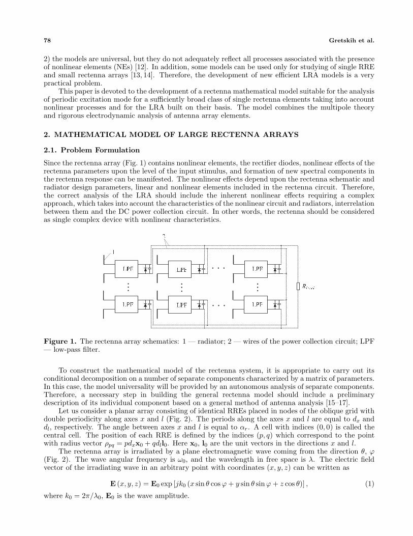
Since the rectenna array (Fig. 1) contains nonlinear elements, the rectifier diodes, nonlinear effects of therectenna parameters upon the level of the input stimulus, and formation of new spectral components inthe rectenna response can be manifested. The nonlinear effects depend upon the rectenna schematic andradiator design parameters, linear and nonlinear elements included in the rectenna circuit. Therefore,the correct analysis of the LRA should include the inherent nonlinear effects requiring a complexapproach, which takes into account the characteristics of the nonlinear circuit and radiators, interrelationbetween them and the DC power collection circuit. In other words, the rectenna should be consideredas single complex device with nonlinear characteristics.

Figure 1. The rectenna array schematics: 1 — radiator; 2 — wires of the power collection circuit; LPF— low-pass filter.

To construct the mathematical model of the rectenna system, it is appropriate to carry out itsconditional decomposition on a number of separate components characterized by a matrix of parameters.In this case, the model universality will be provided by an autonomous analysis of separate components.Therefore, a necessary step in building the general rectenna model should include a preliminarydescription of its individual component based on a general method of antenna analysis [15–17].

Let us consider a planar array consisting of identical RREs placed in nodes of the oblique grid withdouble periodicity along axes x and l (Fig. 2). The periods along the axes x and l are equal to dx anddl, respectively. The angle between axes x and l is equal to αr. A cell with indices (0, 0) is called thecentral cell. The position of each RRE is defined by the indices (p, q) which correspond to the pointwith radius vector ρpq = pdxx0 + qdll0. Here x0, l0 are the unit vectors in the directions x and l.

The rectenna array is irradiated by a plane electromagnetic wave coming from the direction θ, ϕ(Fig. 2). The wave angular frequency is ω0, and the wavelength in free space is λ. The electric fieldvector of the irradiating wave in an arbitrary point with coordinates (x, y, z) can be written as

E (x, y, z) = E0 exp [jk0 (x sin θ cos ϕ + y sin θ sin ϕ + z cos θ)] , (1)

where k0 = 2π/λ0, E0 is the wave amplitude.

Progress In Electromagnetics Research B, Vol. 74, 2017 79

ld

xd

r

(0,-1) (1,-1)

Figure 2. The periodic structure of the rectenna array.

2.2. Large Rectenna Array Schematic

A general block diagram, which allows us to describe various rectenna arrays, is shown in Fig. 3 wherecommon linear subcircuits, LS-1 and LS-2, are separated out in the rectenna. The subcircuit LS-1corresponds to the radiator system, and the subcircuit LS-2 relates to the power collection and loadcircuits. In addition, linear LS-3 and nonlinear subcircuits (NS) combine all linear and nonlinearelements of each RRE.

(LS-2)

(0,0) (p,q)

Figure 3. The block-diagram of the rectenna array.

The division of the block-diagram into subcircuits is determined by several factors, of which thefollowing should be considered. Firstly, in many cases, the rectenna models of different complexity levelsmay be required depending on analysis depth and the accuracy of results. Secondly, the characteristicsof rectenna linear and nonlinear elements differ quite substantially.

The element NS will be presented as a nonlinear 2-Nα-multipole (NM) (Fig. 4(a)), described by themapping �, which maps its input voltage vector unl(t) = (unl1(t), unl2(t), . . . , unlNα(t))T on the currentvector inl(t) = (inl1(t), inl2(t), . . . , inlNα(t))T , i.e.,

inl(t) = �{unl (t)} (2a)

or vice versaunl (t) = �−1 {inl (t)} . (2b)

Here Nα is the number of inputs, which connect the NM with multipole corresponding to subcircuit LS-3(cross-section α-α); superscript T denotes transposition. For each linear subcircuit, we set a one-to-one

80 Gretskih et al.

1

N

()

nlN

ut

1( )nli t

1(

)nl

ut

( )nlNi t

1

N

)(

1U

)(1I

)(

NU

)(NI

1 N

N1

)(1U

)(

1I )(NU

)(

NI

)(1U)(

1I

)(NU

)(

NI

LM-3NM

(a)

(b)

(0,0) (p,q))(RZ

)(

)0,

0( 1xe

)()0,0(1U

)(

)0,

0( 1I

)(

)0,

0( xNe

)()0,0(

NU

)(

)0,

0( NI

)(

),

( 1q

pxe

)(),(1

qpU

)(

),

( 1q

pI

)(

),

(q

p

xNe

)(

),

(q

pNI

1 1N N

)(),( qp

NU

(0,0) (p,q))(LZ

)()0,0(1U

)(

)0,

0( 1I

)()0,0(

NU

)(

)0,

0( NI

)(),(1

qpU

)(

),

( 1q

pI

)(

),

(q

p

NI1 1N N

)(),( qp

NU

(c)

(d)

ω ω

ω ω

ω

ωω ω ω

ω ω ω ω

ω

ω

ω

ω ω

ωω

ω ω

ω ω ω ω

ω ω ω ω

ω ω ω ω

αα

γγ

β

β β

α

α

α

α

αα

γ

γ

γ γ

γγ

γ γ

γ

γγ

α

β

α

β

β

β

β β

ββ

ββ

ββ

Figure 4. The rectenna subcircuits as multipole at the step of determining the state variables.

correspondence between the linear multipoles LM-1, LM-2 and LM-3 (Figs. 4(b), (c), (d)). Unlike theNM, linear multipoles can be described more conveniently in the frequency domain.

Before choosing system parameters describing the linear rectenna multipoles, we will note thefollowing. The procedure of the rectenna analysis can be divided into several stages. This division, aswell as the content of the individual steps is to some extent arbitrary. It depends upon the approachused for the analysis. However, any approach should include a stage of the operating mode selectionfor the analyzed device and a stage of determining its external parameters. These stages for the LRAanalysis are as follows.

At the first stage, according to an infinite array approximation, which will be used below, we assumethat the operating mode of each RRE corresponds to that of the element included into an infinite array.Therefore, the infinite array of the RRE (Nx, Nl → ∞) should be considered on the first step, and hence,the multipoles LM-1, LM-2 have infinite number of inputs. The parameters define the linear multipolesfrom the inputs, which are connected with each other, i.e., relative to the cross-sections α-α, β-β andγ-γ.

At the second stage, the external parameters are defined, and the rectenna is considered asan array with a finite number of RRE (Nx × Nl). Consequently, the multipoles LM-1 and LM-2should be described by finite dimensional matrices. At this stage, the parameters characterizing the

Progress In Electromagnetics Research B, Vol. 74, 2017 81

interaction between the radiator system and external medium must be known, i.e., the complete systemof parameters describing the LM-1 is also required. Therefore, it is quite natural that the systems ofparameters describing linear multipoles can be selected at various stages of analysis. The main criterion,which determines what parameters should be used, is the convenience of their application for specifictasks.

2.3. Analysis of the Nonlinear Regime of the Large Rectenna

Determination of a nonlinear device mode consists in solution of the device state equation [15, 16].Below we will consider some aspects of such a system formation and its features for the LRA.

2.3.1. Description of Linear Multipoles

To form a system of state equations, the multipole LM-1, characterized by an infinite periodic radiatorsystem, can be conveniently described by using the following data: the angular frequency ω, matrix ofself and mutual impedances ZR(ω), and complex amplitudes of the electro-motive force (EMF) eβ(ω)induced at inputs of radiators by the field of the plane wave (Fig. 4(c)). The matrix ZR(ω) for theflat infinite periodic radiator array excited by the plane wave is the infinite block-block-Toeplitz (BBT)matrix, and the external stimulus on the radiator inputs can be represented by the EMF source systemwith a double periodicity. This can be explained as follows. If the external excitation is described byEquation (1), the field intensity of the plane wave in point M00 belonging to the central cell and thefield intensity at the point Mpq are related as

E (Mp,q) = E (M0,0) exp [j (ap + bq)] , (3)

where a = k0dx sin θ cos ϕ, b = k0dl(sin θ cos ϕ cos αr + sin θ sin ϕ sin αr). Therefore, the amplitudes ofEMF induced by the field of the plane wave at the radiators inputs, located in the cells (0, 0) and (p, q)which are converted to the cross-sections β-β (Fig. 3), are related as

e(p,q)β (ω0) = e(0,0)

β (ω0) exp [j (ap + bq)] . (4)

Here e(p,q)β (ω0) and e(0,0)

β (ω0) are the complex amplitude of the radiators EMF arranged in periodicnodes with indices (p, q) and (0, 0), respectively. This relationship describes the system of EMF sourceswith the double periodicity.

The multipole LM-2 (Fig. 4(d)) has an infinite number of inputs and is described by the impedancematrix ZL(ω), which relates the complex current amplitudes I(ω) and the voltages U(ω) at its inputs(cross-section γ-γ) as

U (ω) = ZL (ω) I (ω) . (5)

Here the vectors I(ω) and U(ω) are formed as follows

I (ω) =(. . . , I

(−1,0)1 , I

(−1,0)2 , . . . , I

(−1,0)Nγ

, I(0,0)1 , I

(0,0)2 , . . . , I

(0,0)Nγ

, I(1,0)1 , I

(1,0)2 , . . . , I

(1,0)Nγ

, . . .)T

,

U (ω) =(. . . , U

(−1,0)1 , U

(−1,0)2 , . . . , U

(−1,0)Nγ

, U(0,0)1 , U

(0,0)2 , . . . , U

(0,0)Nγ

, U(1,0)1 , . . . , U

(1,0)Nγ

, . . .)T

.

Let us assume that all RRE are loaded by identical resistors. The multipole LM-3 (Fig. 4(b)),corresponding to subcircuit LS-3 can be described by the impedance matrix which relates the complexamplitudes of the currents and voltages in the cross-sections α-α, β-β, and γ-γ. This relationship canbe written in block form as⎛

⎝ Uα (ω)Uβ (ω)Uγ (ω)

⎞⎠ =

⎛⎝ Z′

αα (ω) Z′αβ (ω) Z′

αγ (ω)Z′

βα (ω) Z′ββ (ω) Z′

βγ (ω)Z′

γα (ω) Z′γβ (ω) Z′

γγ (ω)

⎞⎠

⎛⎝ Iα (ω)

Iβ (ω)Iγ (ω)

⎞⎠ . (6)

Here Ij(ω) = (Ij1(ω), Ij2(ω), . . . , IjNj(ω))T and Uj(ω) = (Uj1(ω), Uj2(ω), . . . , UjNj (ω))T are vectorswhose elements are the complex amplitudes of the currents and voltages at the terminals of LM-3,which are connected to other multipoles (cross-sections α-α, β-β and γ-γ).

82 Gretskih et al.

Thus, relations (2)–(6) completely describe all multipoles, which are included in the generalizedrectenna circuit and are necessary for the formation of state equations. Then we define the matrix ofintrinsic and mutual impedances and the system of the EMF vectors, which describe the entire linearcircuit relative to the cross-sections α-α, where they are connected with the nonlinear multipole. Theseproperties allow us to simplify the solution of state equations for the LRA using approximation of theinfinite rectenna array.

2.3.2. Properties of the Linear Subcircuit of the Infinite Rectenna Array

Let us transform the linear subcircuit of the rectenna, which includes three linear subcircuits (Fig. 3)in such a way that the linear subcircuit LS-3 is unchanged, while subcircuits LS-1 and LS-2 form a newcombined subcircuit coupled to the subcircuit LS-3 in the cross-section σ-σ (Fig. 5).

α

LS-3

α

LS-3

β βββ

Figure 5. The modified linear subcircuit of the rectenna.

Let ZΣ(ω) be the matrix of intrinsic and mutual impedances of the combined multipolecorresponding to the radiators system and DC power collection circuit with respect to the cross-sectionσ-σ. Since the matrices of the multipoles LM-1 and LM-2 are block-block-Toeplitz (BBT) matrices,matrix ZΣ(ω) has the same properties by virtue of the assumption concerning the identical RRE loads.

The matrices of the multiports LM-3 can be presented in the block form

Z (ω) =(

Z′αα (ω) Z′

ασ (ω)Z′

σα (ω) Z′σσ (ω)

), (7)

where Z′ij(ω) are the blocks describing the interaction between the inputs belonging to the cross-sections

i, and j (i, j = α, σ). Taking into account the accepted notation, the matrix of intrinsic and mutualimpedances Zαα(ω) relative to the inputs connected to the nonlinear multipoles (Fig. 5) and the complexEMF amplitudes ex(ω) on the same inputs can be determined from the relations

Zαα (ω) = Z′′αα (ω) − Z′′

ασ (ω)(Z′′

σσ (ω) + ZΣ (ω))−1

Z′′σα (ω) ,

ex (ω) = −Z′′ασ (ω)

(Z′′

σσ (ω) + ZΣ (ω))−1

exσ (ω) ,(8)

where Z′′ij(ω) are infinite-dimensional block-diagonal matrices. The elements of these matrices are the

blocks Z′ij(ω) of the matrices Z(ω). In Eq. (8), vector exσ(ω) is an infinite-dimensional vector formed

as follows

exσ (ω) =(. . . , e(−1,−q)

β (ω) ,0, e(0,−q)β (ω) ,0, . . . , e(−1,0)

β (ω) ,0, e(0,0)β (ω) ,0,

. . . , e(−1,q)β (ω) ,0, e(0,q)

β (ω) ,0, . . .)T

. (9)

Here e(p,q)β (ω) is the vector defined by Eq. (4); 0 is the zero vector whose dimension is equal to the

number of RRE inputs in the cross-section γ-γ. The presence of the zero vector in Eq. (9) reflects the

Progress In Electromagnetics Research B, Vol. 74, 2017 83

fact that the multipole LM-2 does not contain independent sources. Since the diagonal blocks of eachmatrix Z′′

ij(ω) are identical, they are a special case of BBT matrices which, in turn, have the propertiesof circulant matrices. The circulant matrix with complex entries has the following properties:

- if a circulant matrix is non-singular, then its inverse matrix is also circulant;- a set of circulant matrices is a commutative ring;- a set of non-singular circulant matrices is a commutative group under multiplication.

These properties allow us to state that the matrices Zαα(ω) and Z′′ασ(ω)(Z′′

σσ(ω) + ZΣ(ω))−1Z′′σα

(ω) are BBT matrices, while the infinite-dimensional vector ex(ω) whose elements as well as elementsof the vector ex(ω) satisfy relation (4), i.e.,

e(p,q)x (ω) = e(0,0)

x (ω) exp [j (ap + bq)] . (10)

where e(p,q)x (ω) and e(0,0)

x (ω) are the EMF complex amplitudes induced by the incident wave at theterminals of the radiating system converted to the cross-sections α-α of the RREs which are placed incells with numbers (p, q) and (0, 0), respectively. Therefore, the EMF vector in the time domain can bewritten as

e(p,q)x (t) = e(0,0)

x [t + (a/ω) p + (b/ω) q] . (11)

We will show how these properties of the linear subcircuit and EMF vector can be used to solvethe LRA state equations in the approximation of the infinite RRE array.

2.3.3. LRA State Equations

To derive the state equations, we have the following steps:

a) Let Zk,lp,q(ω) be the block of matrix Zαα(ω) describing the interaction between groups of inputs,

which are connected to the nonlinear multipoles RRE (Fig. 6) related to cells with numbers (p, q)and (k, l); the superscripts and subscripts points to rows and columnd defining a position of theblock Zk,l

p,q(ω) in the matrix;b) Let us form a matrix sequence {Zp,q} from elements of the zero row (k = 0, l = 0) of the matrix

Zαα(ω) in the following way

{. . . ,Z−1,−q (ω) ,Z0,−q (ω) ,Z1,−q (ω) , . . . ,Z−1,0 (ω) ,Z0,0 (ω) ,Z1,0 (ω) ,

. . . ,Z−1,q (ω) ,Z0,q (ω) , . . . ,Z1,q (ω) , . . .} , (12)

where Zp,q(ω) = Z0,0p,q(ω);

)(Z

)(

)0,

0( 1t

ex

(0,0)1 ( )nlu t

)()0,0(1 tu

)(

)0,

0( 1t

i

)(

)0,

0(t

exm

(0,0) ( )nlmu t

)()0,0( tum

)(

)0,

0(t

i m

)(

),

( 1t

eq

px

( , )1 ( )p q

nlu t

)(),(1 tu qp

)(

),

( 1t

iq

p

)(

),

(t

eq

pxm

( , ) ( )p qnlmu t

)(),( tu qpm

)(

),

(t

iq

pm

( ) { ( )}nl nlt ti u ( ) { ( )}nl nlt ti u

)(~Z

)(

)0,

0( 1t

ex

(0,0)1 ( )nlu t

)()0,0(1 tu

)(

)0,

0( 1t

i

)(

)0,

0(t

exm

(0,0) ( )nlmu t

)()0,0( tum

)(

)0,

0(t

i m

( ) { ( )}nl nlt ti u= =

ωαα

=

ω

(a) (b)

(0,0) (p,q)

Figure 6. Schematics of the infinite periodic array of the RRE.

84 Gretskih et al.

c) Let us assume that the nonlinear multiports of the RRE are described by relation (2a) and havem = Nα inputs (Fig. 6(a)).

Now consider the representation of current i(p,q)(t) and voltage u(p,q)(t) related to the cell (p, q)which describe the mode of the LS input group and are connected to the nonlinear multipole. Thestate variables, currents or voltages on the nonlinear elements under the periodic input stimuli can berepresented by a Fourier series

i(p,q) (t) =∞∑

n=−∞δnI(p,q)

n exp (jnω0t), (13)

where I(p,q)n is the m-dimensional vector, whose elements are the complex amplitudes of the n-th current

harmonics for LS input groups with (p, q) indices (cross-section α-α); δn = 1 if n = 0 and δn = 1/2if n �= 0. Since the condition in Eq. (11) for the EMF vector is fulfilled, and the matrix of the linearsubcircuit is the BBT matrix, then

i(p,q) (t) = i(0,0) [t + (a/ω0) p + (b/ω0) q] . (14)

The relation between the complex amplitudes of the n-th harmonic currents on the LS inputs withthe indices (p, q) and zero indices (0, 0) can be obtained by comparing formulas (13) and (14)

I(p,q)n = I(0,0)

n exp [jn (ap + bq)] . (15)

The time dependence of the voltage at the same LS inputs can be written as

u(p,q) (t) =∞∑

n=−∞δnU(p,q)

n exp (jnω0t), (16)

where U(p,q)n are complex amplitudes of the n-th harmonic on the LS inputs with the indices (p, q). The

vectors U(p,q)n and I(p,q)

n are related as

U(p,q)n =

∞∑k=−∞

∞∑l=−∞

Zp,qk,l (nω0)I(k,l)

n = Z̃ (nω0) I(p,q)n , (17a)

where

Z̃ (nω0) =∞∑

k=−∞

∞∑l=−∞

Zp,qk,l (nω0) exp {jn [a(k − p) + b(l − q)]}

=∞∑

k=−∞

∞∑l=−∞

Zk,l (nω0) exp {jn [ak + bl]} . (17b)

Consequently,

u(p,q) (t) =∞∑

n=−∞δnZ̃ (nω0) I(p,q)

n exp {jnω0t}. (18)

The resulting representation of i(p,q)(t) and u(p,q)(t) allows us to write down the system of the stateequations for the rectenna as follows

∞∑n=−∞

δnI(p,q)n exp {jnω0t} + �

{ ∞∑n=−∞

δnZ̃ (nω0) I(p,q)n exp {jnω0t} + e(p,q) (t)

}= 0, (19)

for any p, q ∈ −∞,∞; , t ∈ [0, T ]. The solutions of this equation system are the amplitudes of thecurrent harmonics I(p,q)

n for all groups of the LS inputs. All equations of the system are determined fora temporal interval t ∈ [0, T ]. Taking into account relations (14), (15), and (16), we can transform the

Progress In Electromagnetics Research B, Vol. 74, 2017 85

system of equations for the currents at the inputs with the zero indices for any p, q ∈ −∞,∞; t ∈ [0, T ]to

∞∑n=−∞

δnI(0,0)n exp {jnω0 [t + (a/ω0) p + (b/ω0) q]}

+�{ ∞∑

n=−∞δnZ̃ (nω0) I(0,0)

n exp {jnω0 [t + (a/ω0) p + (b/ω0) q]}

+ e(0,0)[t + (a/ω0) p + (b/ω0) q]}

= 0 (20)

for any p, q ∈ −∞,∞; t ∈ [Δt(p,q), T + Δt(p,q)], where Δt(p,q) = (a/ω0)p + (b/ω0)q.One can see that for any p, q ∈ −∞,∞, the determination of the currents I(p,q)

n from the systemin Eq. (19), in which every equation is determined at the interval t ∈ [0, T ], was reduced to solvingthe system of equations with respect to a single vector I(0,0)

n , determined at different temporal intervals(a/ω0)p + (b/ω0)q ≤ t ≤ T + (a/ω0)p + (b/ω0)q. Since all these intervals are equal to the period of thefundamental frequency, it is sufficient to solve Equation (20) only at one of them defined, for example,by indices p = q = 0, i.e.,

∞∑n=−∞

δnI(0,0)n exp {jnω0t} + �

{ ∞∑n=−∞

δnZ̃ (nω0) I(0,0)n exp {jnω0t} + e(0,0) (t)

}= 0, (21)

for any t ∈ [0, T ].Thus, for the given properties of the LS matrix and system of excitation sources, the analysis of the

circuit shown in Fig. 6(a) can be reduced to the analysis of the circuit shown in Fig. 6(b). This circuitconsists of one nonlinear 2m-pole described by the characteristic in Eq. (2a) and one linear multipole,whose impedance matrix is determined at the frequencies of all harmonics and equal to Z̃(nω0) for anyn ∈ (−∞,∞). To analyze such a circuit, one should solve a system of the m(2N + 1)-th order equations(N is the number of retained current harmonics). Consequently, the solution of the state equations ofthe large rectenna in the infinite array approximation is reduced to solve the system of a single equivalentRRE as a part of an infinite array, whose circuit parameters are defined in this subsection. This allowsus to develop an effective method for the rectenna calculation under equi-amplitude excitation by usingavailable algorithms and software solutions for calculating only one RRE. This result is similar to theconcept of a “single” cell known from the theory of linear antenna arrays [18].

2.4. External Parameters of the LRA

2.4.1. Description of the Linear Multipoles

As it was pointed out in Sec. 2.3.1, the linear multipoles at the stage of solving the state equations canbe conveniently characterized by the matrices of intrinsic and mutual impedances. However, externalparameters of the rectenna can be better described by using another approach. At this stage, themultipole LM-1, equivalent to the radiator system can be characterized by the scattering matrix SR(ω),column of the orthonormalized radiation patterns (RP), e(ω, θ, ϕ), column of partial RP, g(ω, θ, ϕ), andorthogonalizing matrix of incidental waves, i.e., to use the descriptions accepted in the matrix theory ofantennas [19]. This is related to the fact that the external parameters of the rectenna for the radiatorsystem can be characterized by the parameters defining its coupling with the external medium. Vectorse(ω, θ, ϕ) and g(ω, θ, ϕ) are just the required parameters.

Matrix SR(ω) connects the amplitudes of incidental a′′(ω) and reflected b′′(ω) waves at the inputsof the radiator system (the cross-section β-β, Fig. 7(a)) and the amplitudes of the convergent u′

d(ω0)and the divergent u′

d(ω) spherical waves in the free space channels (cross-section δ-δ)(b′′ (ω)u′

d (ω)

)=

(Sββ Sβδ

Sδβ Sδδ

)(a′′ (ω)u′

c (ω0)

). (22)

86 Gretskih et al.

)(b)(a

1 N

)(b)(a

1 N

1

N

)(1u

)(Nu

)(Ni

)(1i

)(Q

ω ω

ω

ω

ω

ω

ω

ω ω

ββα

γγ

αγ

γγ

α α

α α

α

α

β β

β

(c)

)(LS

)(0b')(0a'

N N

)(RS

( )du'0( )cu'

N N

)(b'')(a''

NN

ω ω

δ

ω

ωω

β

γ

δ

β

ω ωγ

ω

γγ

δ δ

ββ

(a)

(b)

(0,0) (p,q)

Figure 7. The representation of the linear rectenna subcircuits at the stage of the external parameterdefinition.

Vector u′c(ω0) is related to the electric field intensity E(ω0, θ, ϕ) of the exciting flat wave coming

from the direction (θ, ϕ) in the following way

u′c(ω0) = − −jλ0√

2W0E(ω0, θ, ϕ)e(ω0, θ, ϕ) = − −jλ0√

2W0E(ω0, θ, ϕ)AT (ω0)g(ω0, θ, ϕ) (23)

where W0 is the wave impedance of the free space. In Equation (23), we take into account the relationsbetween e(ω0, θ, ϕ), g(ω0, θ, ϕ) and A(ω) which are determined by the relation proposed in [19]

e(ω, θ, ϕ) = AT (ω)g(ω, θ, ϕ). (24)

Multipole LM-2, which defines the energy receivers connected to the rectenna, is characterized bythe scattering matrix SL(ω) relating complex amplitudes of the incident a′

0(ω) and reflected b′0(ω) waves

on its inputs (cross-section γ-γ, Fig. 7(b))

b′0 (ω) = SL (ω)a′

0 (ω) . (25)

Let us define the linear multipole LM-3 by the mixed matrix Q(ω), which relates (see Fig. 7(c))the incidental and reflected waves in the cross-sections β-β and δ-δ to the normalized currents iα(ω)and voltages uα (ω) in the cross-section α-α, which connects LM-3 and the nonlinear multipole.⎛

⎝ uα (ω)bβ (ω)bγ (ω)

⎞⎠ =

⎛⎝ Qαα (ω) Qαβ (ω) Qαγ (ω)

Qβα (ω) Qββ (ω) Qβγ (ω)Qγα (ω) Qγβ (ω) Qγγ (ω)

⎞⎠

⎛⎝ iα (ω)

aβ (ω)aγ (ω)

⎞⎠ (26)

The blocks of matrix Q(ω) can be calculated if the scattering matrix S(ω) of the multipole LM-3is known. This relation can be found in [15, 16].

The normalized currents iα(ω) and voltages uα(ω) are related to the complex voltage amplitudesUα(ω) by the known relations

iα (ω) = 0.5 {Zw}1/2 Iα (ω) ,

uα (ω) = 0.5 {Zw}−1/2 Uα (ω) ,

where {Zw}1/2 and {Zw}−1/2 are the diagonal matrixes with the elements defined as numbers√

Zwl(ω)(for {Zw}1/2) and 1/

√Zwl(ω) (for {Zw}−1/2); Zwl(ω) is the wave impedance at the frequency ω of the

transmission line connected in the cross-section αα to the l-th input of the nonlinear multipole. In what

Progress In Electromagnetics Research B, Vol. 74, 2017 87

follows, we assume that the wave impedances of all lines are equal, i.e., Zwl(ω) = Zw(ω) (l = 1, . . . , Nα).Calculation of the external rectenna parameters requires that the following initial data should be given:the operating frequency ω0, vector of the input stimuli u′

c(ω0), parameters of the multipoles includedinto the system, and complex current amplitudes I(p,q)

n , obtained by solving the state equations, whichdetermine the normalized currents iα(ω) at the frequency of the n-th harmonic in the cross-section α-αof all RRE arrays which are related as√

Zwiα (nω0) =(. . . , I(−1,−q)

n , I(0,−q)n , I(1,−q)

n , . . . , I(−1,0)n , I(0,0)

n , I(1,0)n , . . . , I(−1,q)

n , I(0,q)n , I(1,q)

n , . . .)T

. (27)

2.4.2. Rectenna Parameters

The external parameters of the rectenna at frequency ω can be derived by determining the vectors a′0(ω)

and u′d(ω) for the given input stimuli u′

c(ω0) and the known vector iα(ω) found as solution of the stateequations. In what follows, ω stands for any frequency nω0 for n = 0, 1, . . . if further clarification is notnecessary. The parameters of a linear subcircuit will be presented by the mixed matrix QA(ω) whosedefinition and relations for calculating its blocks using the parameters LM-1, LM-2 and LM-3 are givenin [15, 16]. Relations, which describe the relationship between vectors a′

0(ω), u′d(ω) and vectors u′

c(ω0),iα(ω), can be written as follows

a′0(ω) = QA

γα(ω)iα(ω0) +{

QAγδ(ω0)u′

c(ω0) if ω = ω0

0 if ω �= ω0, (28)

u′d(ω) = Q̃δα(ω)iα(ω0) +

{Q̃δδ(ω0)u′

c(ω0) if ω = ω0

0 if ω �= ω0. (29)

The obtained expressions represent a system of output equations describing the reactions of thegeneralized rectenna circuit (Fig. 2), in the cross-sections γ-γ and δ-δ where NM is represented bythe equivalent current sources iα(ω). The currents are determined by solving the state equations usingexternal stimuli u′

c(ω0).Relations (28) and (29) are formally defined as linear relations, connecting the vector of input

parameters and vectors u′c(ω0) and iα(ω). However, the nonlinear dependency of iα(ω) upon

u′c(ω0), described by the state equations, results in a nonlinear dependency of the input parameters

{a′0(ω),u′

d(ω)}T on the input stimuli u′c(ω0). This results in a nonlinear dependency of all the external

rectenna parameters on the input stimuli. Therefore, if the rectenna should be characterized by someinput parameters, it is necessary to specify a level of input stimuli for which the given level is obtained.In addition, the nonlinear rectifier diodes give rise to new spectral components in the current spectrumiα(ω) at the inputs (α-α) of the linear subcircuit whose frequencies ω differ from the frequencies of inputstimuli ω0. At these frequencies u′

c(ω �= ω0) ≡ 0, therefore relations (28) and (29) can be simplified

a′0(ω) = QA

γα(ω)iα(ω0), (30)

u′d(ω) = Q̃δα(ω)iα(ω0). (31)

Let us determine the external key parameters of the rectenna: the DC voltages and currents in theload, DC power absorbed by the multipole load, rectenna COP, and field reradiated by the rectennaat the fundamental frequency and its upper harmonics. The parameters are calculated in the followingway.

We assume that the DC connections between RREs within the boundaries of the rectenna apertureare of the same type. Based on this assumption, we can determine the DC current and voltage at thearray load. For the series collection scheme, we have

U0 = N0U0RRE , I0 = I0RRE . (32)

The voltage and current for the parallel collection scheme are related as

U0 = U0RRE , I0 = N0I0RRE . (33)

Here U0RRE , I0RRE are the voltage and current in a load of a single RRE; U0, I0 are the voltage andcurrent in the load of the rectenna when the number of RREs is N0.

88 Gretskih et al.

The collection scheme of same type (either parallel or series) under an equi-amplitude excitation ofthe large rectenna is optimal in a sense that the COP of this collection schemes is equal to one under acondition that the loads of the RRE are equal at the main frequency and its upper harmonics. This factfollows from identity of the characteristics of all the rectenna RREs as sources of DC voltage. At thesame time, the load impedances, which are required to achieve the maximum, COP of the RRE and,hence, the maximal COP of the rectenna for the series and parallel collection schemes can be different.Options for the optimal collection schemes are not limited by the only one type of RRE connections.For example, all the serial and parallel circuits of a hierarchical type, which at any hierarchy level hasthe same number of combined elements (parallel or series) will also have the COP equal to one [20].

The DC power absorbed in the multipole load can be calculated as

P0 = a′∗T0 (ω)(E − S∗T

L (ω)SL(ω)) a′0(ω)

∣∣ω→0

. (34)

Here vector a′0(ω)|ω→0 is defined from Equation (30), a′

0(ω)|ω→0 = QAγα(nω0)iα(nω0)|n=0, and E is the

unit matrix.The rectenna COP is defined as the ratio between power P0 and maximal power PM that can be

harvested from the incident field by the radiator system if the load is optimal

η =P0

PM=

P0

u′∗Tc (ω0)u′

c(ω0)=

2W0P0

λ20|E|2g∗T (ω0, θ, ϕ)A∗(ω0)AT (ω0)g(ω0, θ, ϕ)

(35)

When the rectenna is excited by an electromagnetic wave with a frequency ω0, the secondaryfield ES is formed in the surrounding space. The scattered field in the wave zone at the fundamentalfrequency can be represented by two terms [19]

ES (ω0, θ, ϕ) = EΣ (ω0, θ, ϕ) + EC (ω0, θ, ϕ)

=√

2W0a′′T (ω0)g (ω0, θ, ϕ)

exp (−jk0r)r

+ EC (ω0, θ, ϕ) , (36)

where EΣ(ω0, θ, ϕ) is the secondary field initiated by the current flow at the terminals of the rectennaradiators, and EC(ω0, θ, ϕ) is the field scattered by the matched radiators and design elements, a′′

(ω0)if the incident wave at the inputs of rectenna radiators is defined as

a′′ (ω) =(E − SββQ̃ββ

)−1(SββQ̃βαiα (ω) +

{Sβγu′

c (ω0) if ω = ω0

0 if ω �= ω0

). (37)

The matrices Q̃ij are computed by using the parameters of the linear multiport as

Q̃ij = Qij + Qiγ (E − SLQγγ)−1 SLQγj, i = α, β; j = α, β. (38)

At the frequencies of upper harmonics, the radiators of the rectenna are excited from the side of theinput terminals. Therefore, the scattering field at the frequencies ωn = nω0 has only one component,EΣ(ωn, θ, ϕ). The scattered field in the far zone at the fundamental frequency and its upper harmonicsis determined by the expression [19]

ES(ωn, θ, ϕ) =√

2W0a′′T (ωn)g (ωn, θ, ϕ)

exp (−jnk0r)r

. (39)

Since all RRE parameters under equiamplitude excitation are identical, formula (39) can berepresented as follows

ES (ωn, θ, ϕ) =√

2W0a′′T0 (ωn)g0 (ωn, θ, ϕ)F (ωn, θ, ϕ)

exp (−jnk0r)r

, (40)

where a′′0t(ωn) and g0(ωn, θ, ϕ) are the amplitude of the incidental waves and the partial RP of the

RREs radiator at the frequency of the n-th harmonic, and F (ωn, θ, ϕ) is the array multiplier at thesame frequency.

If the parameters of the RRE radiators are defined, the field ES(ωn, θ, ϕ) can be easily calculated.

Progress In Electromagnetics Research B, Vol. 74, 2017 89

3. MODEL VERIFICATION

As shown in Subsection 2.3.3, the nonlinear mode of the LRA excited by periodic fields can be studiedby examining the mode of one equivalent RRE operating in the infinite array. This approach hasallowed us to develop the effective algorithm for simulation of electrodynamic and energy characteristicof the rectenna structures and DC power collection circuits which take into account nonlinear effects.A software package for simulation of the rectenna system whose radiating structure is a periodic planararray of microstrip radiators with arbitrary geometry was implemented based on the proposed method

To determine the reliability of the developed technique, the rectenna experiments were performedby wireless energy transmission using microwave beams. The transmitting equipment of the WPTsystem consisted of a microwave generator, which was placed outside the anechoic chamber, and amirror antenna. The generator was working at 2.45 GHz.

The rectenna developed for the model verification consists of nine single-type modules (Fig. 8(a)).The design of these base module with dimensions of 0.7m × 0.7 m allowed us to easily increase therectenna aperture. Fig. 8(b) shows a schematic diagram of the base module, which consists of 16 RREs(eight parallel strips with the RRE tandem). The module elements were placed at the nodes of atriangular grid with spacing equal to λ/2.

(a) (b)

Figure 8. The experimental rectenna: (a) design; (b) the schematic diagram of the base module.

Loop vibrators over a screen were used as antennas; two opposite connected diodes 3A208A withpower-carrying capacity of 0.5 watts were connected to each vibrator. The vibrators were resonantlytuned taking into account the diodes capacitance. Decoupling between the rectifier and DC circuits inthe RRE was carried out by connecting the wires of the power collection circuit to the point of zeropotential of the loop vibrator. The printed-circuit board of the module foil-clad was made of a glassfiber laminate (εr = 6) whose thickness was 2 mm, placed at a height of 9mm over the screen. Therectenna consisted of 144 RREs.

The rectenna was designed so that the modules can be DC interconnected in series, parallel orseries-parallel. A separate load resistor can be connected to each module.

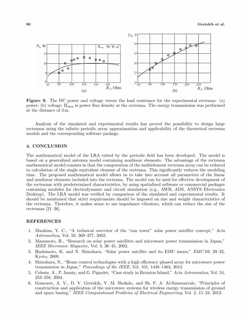
The experimental and simulated results are presented in Fig. 9, where the DC power (Fig. 9(a))and voltage (Fig. 9(b)) are plotted versus load resistance. The experimental and simulated resultsare marked by circles and solid lines, respectively. For the optimal load resistance RLopt = 120 Ohm,obtained from Fig. 9(a), the rectification COP was also measured and equals 87.9%. The relativemeasurement error was Δm ± 19.5%.

90 Gretskih et al.

R , OhmL R , OhmL(a) (b)

Figure 9. The DC power and voltage versus the load resistance for the experimental rectenna: (a)power; (b) voltage; Πmax is power flux density at the rectenna. The energy transmission was performedat the distance of 3 m.

Analysis of the simulated and experimental results has proved the possibility to design largerectennas using the infinite periodic array approximation and applicability of the theoretical rectennamodels and the corresponding software package.

4. CONCLUSION

The mathematical model of the LRA exited by the periodic field has been developed. The model isbased on a generalized antenna model containing nonlinear elements. The advantage of the rectennamathematical model consists in that the computation of the multielement rectenna array can be reducedto calculation of the single equivalent element of the rectenna. This significantly reduces the modelingtime. The proposed mathematical model allows us to take into account all parameters of the linearand nonlinear elements included into the rectenna. The model can be used for effective development ofthe rectennas with predetermined characteristics, by using spatialized software or commercial packagescontaining modules for electrodynamic and circuit simulation (e.g., AWR, ADS, ANSYS ElectronicsDesktop). The LRA model was verified by comparison of the simulated and experimental results. Itshould be mentioned that strict requirements should be imposed on size and weight characteristics ofthe rectenna. Therefore, it makes sense to use impedance vibrators, which can reduce the size of therectennas [21–26].

REFERENCES

1. Mankins, Y. C., “A technical overview of the “sun tower” solar power satellite concept,” ActaAstronavtica, Vol. 50, 369–377, 2002.

2. Masumoto, H., “Research on solar power satellites and microwave power transmission in Japan,”IEEE Microwave Magazine, Vol. 3, 36–45, 2002.

3. Hashimoto, K. and N. Shinohara, “Solar power satellite and its EMC issues,” EMC’09, 29–32,Kyoto, 2009.

4. Shinohara, N., “Beam control technologies with a high efficiency phased array for microwave powertransmission in Japan,” Proceedings of the IEEE, Vol. 101, 1448–1463, 2013.

5. Celeste, A., P. Jeanty, and G. Pignolet, “Case study in Reunion Island,” Acta Astronautica, Vol. 54,253–258, 2004.

6. Gomozov, A. V., D. V. Gretskih, V. M. Shokalo, and Sh. F. A. Al-Sammarraie, “Principles ofconstruction and application of the microwave systems for wireless energy transmission of groundand space basing,” IEEE Computational Problems of Electrical Engineering, Vol. 2, 15–23, 2012.

Progress In Electromagnetics Research B, Vol. 74, 2017 91

7. Dickinson, R. M., “Power in the sky: Requirements for microwave wireless power beamers forpowering high-altitude platforms,” IEEE Microwave Magazine, Vol. 14, 36–47, 2013.

8. Wu, Y., J. Linnartz, et al., “Modeling of RF energy scavenging for batteryless wireless sensorswith low input power personal indoor and mobile radio communications,” PIMRC, IEEE 24thInternational Symposium, 527–531, 2013.

9. Lu, X., P. Wang, D. Niyato, et al., “Wireless networks with RF energy harvesting: A contemporarysurvey,” IEEE Communications Surveys and Tutorials, Vol. 17, 757–789, 2015.

10. Kotter, D. K., S. D. Novack, W. D. Slafer, and P. J. Pinhero, “Theory and manufacturing processesof solar nanoantenna electromagnetic collectors,” Journal of Solar Energy Engineering-transactionsof the Asme, Vol. 132, 2010, http://www.academia.edu/8220294.

11. Bankov, S. E., “Signal detection in a radiating nonlinear electromagnetic crystal,” Journal of RadioElectronics, No. 1, 2012, http://jre.cplire.ru/jre/jan12/1/text.pdf (in Russian).

12. Semenikhina, D. V., A. I. Semenikhin, T. Y. Privalova, and V. V. Demshevsky, “Parametricalexcitation microstrip lattice with nonlinear loads,” International Conference on Electromagneticsin Advanced Applications (ICEAA), 245–248, 2014.

13. Huang, W., B. Zhang, X. Chen, K. Huang, and C. Liu, “Study on an S-band rectenna array forwireless microwave power transmission,” Progress In Electromagnetics Research, Vol. 135, 747–758,2013.

14. Matsunaga, T., E. Nishiyama, and I. Toyoda, “5.8-GHz stacked differential rectenna suitable forlarge-scale rectenna arrays with DC connection,” IEEE Trans. Antennas and Propag., Vol. 63,5944–5949, 2015.

15. Shifrin, Ya. S. and A. I. Luchaninov, “Antennas with nonlinear elements,” The Reference Manualon Antenna Equipment, Vol. 1, 207–235, Moscow, 1997 (in Russian).

16. Luchaninov, A. I. and Y. S. Shifrin, “Mathematical model of antenna with lumped nonlinearelements,” Telecommunications and Radio Engineering, Vol. 66, No. 9, 763–803, 2007.

17. Shifrin, Y. S., A. I. Luchaninov, and A. S. Posokhov, “Structural model of antennas with nonlinearelements,” Telecommunications and Radio Engineering, Vol. 59, Nos. 1–2, 32–48, 2003.

18. Amitay, N., V. Galindo, and C. P. Wu, Theory and Analysis of Phased Array Antennas, JohnWiley & Sons Inc, New York, 1972.

19. Sazonov, D. M., Multi-element Antenna Systems, Matrix Approach, Publishing House“Radiotekhnika”, Moscow, 2015 (in Russian).

20. Shokalo, M. V., A. I. Luchaninov, A. M. Rybalro, and D. V. Gretskih, “Large-aperture rectifyingantennas for wireless energy transfer by a microwave beam,” Kollegium, Kharkov, 2006 (in Russian).

21. Nesterenko, M. V., V. A. Katrich, and V. M. Dakhov, “Formation of the radiation field with theset spatial-polarization characteristics by the crossed impedance vibrators system,” Radiophysicsand Quantum Electronics, Vol. 53, 371–378, 2010.

22. Nesterenko, M. V., V. A. Katrich, Y. M. Penkin, V. M. Dakhov, and S. L. Berdnik, Thin ImpedanceVibrators. Theory and Applications, Springer Science+Business Media, New York, 2011.

23. Nesterenko, M. V., V. A. Katrich, V. M. Dakhov, and S. L. Berdnik, “Impedance vibrator witharbitrary point of excitation,” Progress In Electromagnetics Research B, Vol. 5, 275–290, 2008.

24. Nesterenko, M. V., “Analytical methods in the theory of thin impedance vibrators,” Progress InElectromagnetics Research B, Vol. 21, 299–328, 2010.

25. Nesterenko, M. V., V. A. Katrich, S. L. Berdnik, Y. M. Penkin, and V. M. Dakhov, “Applicationof the generalized method of induced EMF for investigation of characteristics of thin impedancevibrators,” Progress In Electromagnetics Research B, Vol. 26, 149–178, 2010.

26. Penkin, Yu. M., V. A. Katrich, and M. V. Nesterenko, “Development of fundamental theory of thinimpedance vibrators,” Progress In Electromagnetics Research M, Vol. 45, 185–193, 2016.