Mathematical Economics - 14.139.185.6
84
M M Ca M MA AT TH H UN SC alicut Univ H HE E M MA A COM B.S NIVER CHOOL O versity P. A AT TI I C C A A MPLEMENT Sc. Mat II SEME RSITY OF DISTA O. Malap 4 A AL L E EC C TARY COU themat ESTER OF CA ANCE ED puram, K 420 C CO ON NO O URSE tics ALICU DUCATIO Kerala, Ind O OM MI I C CS S UT ON dia 673 6 S S 635
Transcript of Mathematical Economics - 14.139.185.6
MM
Ca
MMAATTHH
UN
SC
alicut Univ
HHEEMMAA
COM
B.S
NIVER
CHOOL O
versity P.
AATTIICCAA
MPLEMENT
Sc. Mat
II SEME
RSITY
OF DISTA
O. Malap
4
AALL EECC
TARY COU
themat
ESTER
OF CA
ANCE ED
puram, K
420
CCOONNOO
URSE
tics
ALICU
DUCATIO
Kerala, Ind
OOMMIICCSS
UT
ON
dia 673 6
SS
635
School of Distance Education
Mathematical Economics 2
UNIVERSITY OF CALICUT SCHOOL OF DISTANCE EDUCATION
Study Material
BSc. Mathematics
II Semester
Complementary Course
MATHEMATICAL ECONOMICS
Prepared by: Dr. K.X. Joseph Director Academic Staff College University of Calicut
Scrutinised by : Sri. C.P. Mohammed (Retd.)Poolakkandy House Nanmanda P.O. Calicut District
Layout: Computer Section, SDE ©
Reserved
School of Distance Education
Mathematical Economics 3
CONTENTS
MODULE I : INEQUALITIES IN INCOME 5
UNIT 1: INCOME INEQUALITY
EXERCISES
MODULE II : LINEAR PROGRAMMING 11 UNIT 1: LINEAR PROGRAMMING
UNIT 2: GRAPHICAL SOLUTION
UNIT 3: SIMPLEX METHOD
EXERCISES
MODULE III : THEORY OF GAMES 56 UNIT 1: GAME THEORY
UNIT 2: LINEAR PROGRAMMING SOLUTION OF GAMES
EXERCISES
MODULE IV : INPUT OUTPUT ANALYSIS 73
UNIT 1: INTRODUCTION
UNIT 2: INPUT-OUT PUT MODEL
EXERCISES

School of Distance Education
Mathematical Economics 4
School of Distance Education
Mathematical Economics 5
Module I
INEQUALITIES IN INCOME
UNIT 1: INCOME INEQUALITY
According to Frank. A. Cowell “Inequality is in itself an awkward word, as well as one used in connection with a number of awkward social and economic problems. The difficulty is that the word can trigger quite a number of different ideas in the mind of a reader or listener, depending on his training and prejudices”.
The term inequality obviously suggests a departure from some idea of equality. In our society there are differences among people in terms of asset ownership, land holdings, income etc. The measures of inequality addresses to measure the degree and magnitude of inequality of variables.
There are different methods for measuring inequality in variables. The important graphical methods are frequency table graphs and Lorenz Curve. Range, Mean deviation, Coefficient of variation, Gini concentration ratio, Pareto distribution and lognormal distribution are the other inequality measures.
Income may be defined as the increase in a personal command over resources during a given time period. By income inequality we mean a scalar representation of the interpersonal differences in income with in a given population.
Method of Measuring Inequality
Most of the results in inequality measurement and many inequality indices themselves are based on the Lorenz curve for an income distribution. Here we confined to the construction of Lorenz curve for an empirical data only without giving mathematical equivalence.
LORENZ CURVE
Lorenz curve is a graphical representation to study the variation in a distribution like income, profit, wealth etc. It is named after Max O Lorenz who designed it to study the concentration of wealth or income. Like ogive it is in the form of cumulative frequency curve. Here the cumulative percentages of X and Y to the totals are taken along the X and Y axis. If the percentage number of persons are plotted on the X axis and the percentage of total incomes along the Y axis the graph so obtained is called the Lorenz Curve. The Lorenz curve is compared with a line of equal distribution which is a straight line joining 0 with 100 percent. This line indicates that if all the persons in a particular town were possessing equal wealth, then 5% of them would have 5% of wealth, 40% of them would have 40% of wealth and so on. The more Lorenz curve is away from the line of equal distribution, the greater the inequality of income or wealth amongst the persons.
School of Distance Education
Mathematical Economics 6
Measuring Income Inequality
Inequality in the distribution of income and wealth in a society can often be inferred by mere inspection. The nature and sources of inequality and how latter affects the lives of people have been studied elaborately by calculating various social indices.
A visually appealing way of representing the inequality of income distribution is obtained by plotting the cumulative share in total income against the cumulative proportion of the population with income not exceeding a given level, for every level of income. This is called Lorenze Curve.
The Lorenze curve corresponding to the distribution in which every one receives the same income is the line OD, which is referred to as the line of ‘perfect equality’. There are several inequality indices which attempt to measure the divergence between the Lorenze Curve for a given income distribution and the line of perfect equality. The best known and most widely used among these is the Gini coefficient.
Gini Coefficient
The Gini coefficient G is defined as the area between the Lorenze Curve and the line of equality divided by the area of the triangle below this line. The Gini coefficient varies from 0 to 1.
A variant of the Gini coefficient given by Prof. Amartya Sen is given below. Suppose there are ‘n’ individuals or households who are arranged in ascending order of their income as y1 < y2 < y3 <… < yn Sen defines Gini coefficient as
G = 1+µn
2n1
2− [ny1 + (n –1) y2… + 2yn –1 + 1yn]
where µ is the average income. This form makes clear the income weighting scheme so that the poorest person receives a weight of ‘n’ and the richest person a weight of unit.
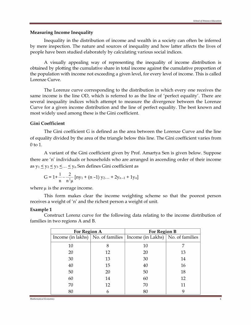
Example 1 Construct Lorenz curve for the following data relating to the income distribution of families in two regions A and B.
For Region A For Region B Income (in lakhs) No. of families Income (in Lakhs) No. of families
10 20 30 40 50 60 70 80
8 12 13 15 20 14 12 6
10 20 30 40 50 60 70 80
7 13 14 16 18 12 11 9
School of Distance Education
Mathematical Economics 7
Solution
For Region A
Mid Value fA Total value of x Cum value of x % cum. value Cum. fA % Cum. fA
10 20 30 40 50 60 70 80
8 12 13 15 20 14 12 6
80 240 390 600
1000 840 840 400
80 320 710
1310 2310 3150 3990 4470
1.78 7.16
15.88 29.30 51.67 70.47 89.26
100.00
8 20 33 48 68 82 94
100
8 20 33 48 68 82 94
100
For Region B Mid Value fA Total value of x Cum value of x % cum. value Cum. fB % Cum. fB
10 20 30 40 50 60 70 80
8 13 14 16 18 12 11 9
70 260 420 640 900 720 770 720
70 330 750
1390 2290 3010 3780 4500
1.55 7.33
16.66 30.88 50.88 66.88 84.00
100.00
7 20 34 50 68 80 91
100
7 20 34 50 68 80 91
100
10 20 30 40 50 60 70 80 90 100
10
0
20
30
40
50
60
70
80
90
100
Sample A
Sample B
% cum. freq.
% c
um. v
alue
.
Line of Equality
Y
X
School of Distance Education
Mathematical Economics 8
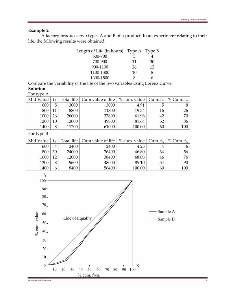
Example 2 A factory produces two types A and B of a product. In an experiment relating to their life, the following results were obtained.
Length of Life (in hours) Type A Type B 500-700 5 4 700-900 11 30 900-1100 26 12 1100-1300 10 8 1300-1500 8 6
Compare the variability of the life of the two variables using Lorenz Curve. Solution For type A Mid Value fA Total life Cum value of life % cum. value Cum. fA % Cum. fA
600 800
1000 1200 1400
5 11 26 10 8
3000 8800
26000 12000 11200
3000 11800 37800 49800 61000
4.91 19.34 61.96 81.64
100.00
5 16 42 52 60
8 26 70 86
100 For type B Mid Value fA Total life Cum value of life % cum. value Cum. fA % Cum. fA
600 800
1000 1200 1400
4 30 12 8 6
2400 24000 12000 9600 8400
2400 26400 38400 48000 56400
4.25 46.80 68.08 85.10
100.00
4 34 46 54 60
6 56 76 90
100
X 10 20 30 40 50 60 70 80 90 100
10
0
20
30
40
50
60
70
80
90
100
Sample A
Sample B
% cum. freq.
% c
um. v
alue
.
Line of Equality
Y
School of Distance Education
Mathematical Economics 9
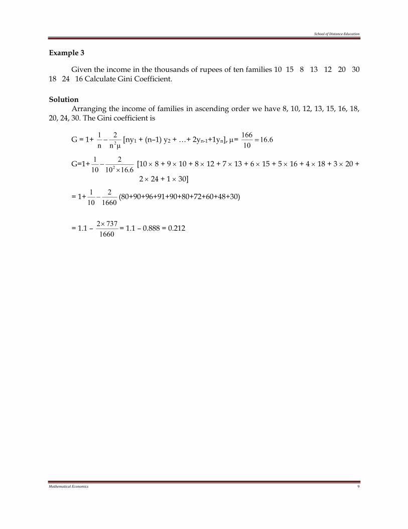
Example 3
Given the income in the thousands of rupees of ten families 10 15 8 13 12 20 30 18 24 16 Calculate Gini Coefficient.
Solution Arranging the income of families in ascending order we have 8, 10, 12, 13, 15, 16, 18, 20, 24, 30. The Gini coefficient is
G = 1+ µn
2n1
2− [ny1 + (n–1) y2 + …+ 2yn-1+1yn], µ= 6.1610
166=
G=1+6.1610
2101
2 ×− [10 × 8 + 9 × 10 + 8 × 12 + 7 × 13 + 6 × 15 + 5 × 16 + 4 × 18 + 3 × 20 +
2 × 24 + 1 × 30]
= 1+1660
2101− (80+90+96+91+90+80+72+60+48+30)
= 1.1 – 1660
7372× = 1.1 – 0.888 = 0.212
School of Distance Education
Mathematical Economics 10
EXERCISES
II. Very Short Answer Questions
1. What is a Lorenz Curve? 2. Define Gini index. 3. What are the causes of inequality in income? 4. Define income inequality. 5. How will you construct Lorenz Curve? 6. What are the measures to be taken to reduce income inequality? 7. Calculate Gini index given the income of 10 persons as 72, 100, 30, 45, 150, 86, 110, 60, 94,
35.
IV. Long Answer Questions 8. From the following table giving data regarding income of workers in two factories, draw
a graph (Lorenz Curve) to show which factory has greater inequalities of income. Income Rs Below 500 500-1000 1000-2000 2000-3000 3000-4000 Factory A 6000 4250 3600 1500 650 Factory B 5000 4500 4800 2200 1500
9. Draw a Lorenz Curve for the following data Profit (in lakhs) : 10 15 20 25 30 35 Factory A : 4 12 15 18 9 3 Factory B : 8 15 28 25 10 2
School of Distance Education
Mathematical Economics 11
Module II
LINEAR PROGRAMMING
UNIT 1: LINEAR PROGRAMMING
Linear programming (LP) is one of the most widely used and best understood Operations Research Techniques. The LP is concerned with the problem of allocating limited resources among the competing activities in an optimal manner. This type of problem arises in a number of situations such as manufacturing an item at a minimum cost, blending of chemicals, allocating salesmen to sales territories, selection of various media for advertising campaign, scheduling production etc.,
LP had its origin in the input output analysis developed by the economists Leonteif and Hitchcock. Koopman studied: ‘Transportation type problems’ during 1940s and Stigler discussed ‘diet problem’ in 1945. However Prof. George B. Dantzig is responsible for the development of the popular approach “simplex method”, a systematic procedure for solving LP problem. The early applications of LP technique were for solving military logistics problems. However, it was soon carried over into the government sector, business and industry and non-profit organizations. Immediately it was found to be a powerful technique for managerial decision problems in business. The development and use of computers have increased the utility of LP technique in the recent years.
Basic requirements of LP problems.
Regardless of the nature of the problem, the use of LP technique should meet the following basic requirements.
i. Well defined objection function: A linear programming problem (LPP) must have a well defined objective function. The objective function may be to maximize the contribution by utilizing the available resources or it may be to produce at the lowest possible cost by using the limited amount of production factors with in a certain time period.
ii. Limited resources: The availability of resources is limited. If the resources are not limited, then the problem cannot be considered as a managerial decision making problem. These limited resources may be production capacity, skilled workers, money, technology etc., These limited resources are usually expressed as constraints in an LPP.
iii. Decision variables and their relationships: Linear programming technique is most useful when the problem involves a large number of decision or activity variables which are interrelated in terms of utilization of the available resources. All decision variables in a LPP are continuous, controllable and non-negative.
iv. Alternative courses of action: The problem must have alternative courses of action. For example, it may be possible to make a selection between various combination of manpower, machine-hours and money or it may be possible to allocate manufacturing capacities in a certain ratio for manufacturing various products.
School of Distance Education
Mathematical Economics 12
Assumptions of LP:
i. Certainty: In LP models, all model coefficients such as unit profit contribution of each product, the quantity of resources required per unit production etc., are assumed to be known with certainty. However, in some cases these may be either random variables following a probability distribution or tend to change. Such problems can be solved using stochastic LP model or parametric programming. Sensitivity analysis in LP can handle the uncertain situations to a considerable limit.
ii. Divisibility or Continuity: The solution values of decision variables and resources are assumed to have either whole integers or mixed numbers (integers and fractionals). However, if only integer variables are desired (for ex: machines, men, etc.,) then another technique called integer programming is used to obtain non-fractional or integer solutions to decision variables.
iii. Additivity: The additivity in LP means that the total sum of the resources used by different activities must be equal to the sum of the resources used by each activity individually. Further the value of the objective function for the given values of decision variables must equal to the sum of the resources used by each activity individually. Further the value of objective function for the given values of decision variables must equal to the sum of the contributions earned from each decision variable. This simply means that the total profit from the sale of two products must be equal to the sum of profits earned separately from the two products.
iv. Linearity: The primary requirement of a linear programming problem is that the objective function and the constraints governing it, should be linear in form. ‘Linear’ implies that the relationships among the decision variables must be directly proportional. The proportionality requires that the measure of outcome and usage of resources must be proportional to the level of each activity.
Formulation of LPP
In formulating a linear programming problem, it is necessary to specify (i) decision variables (ii) the objective function and (iii) constraints. The decision variables are the variables for which a decision is required to be taken.
We explain these concepts using the following examples.
Example 1
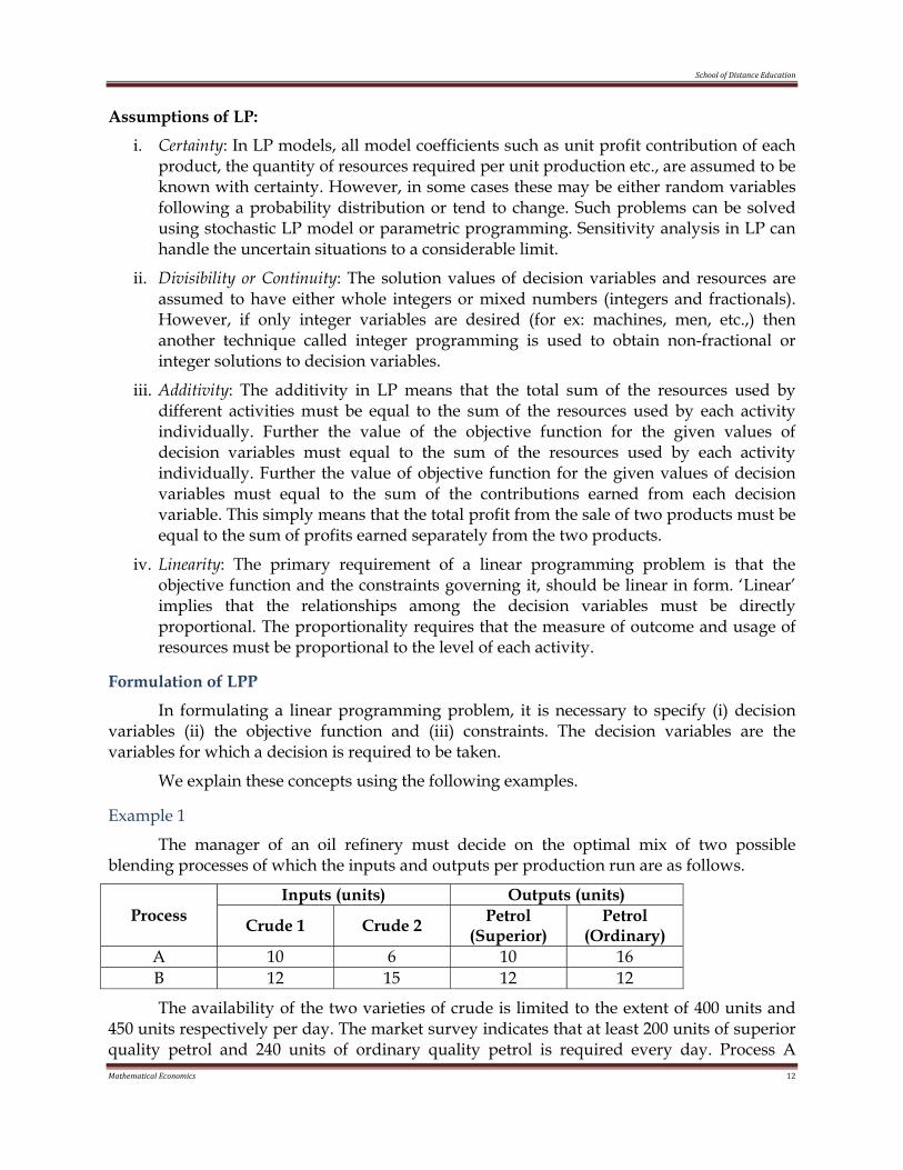
The manager of an oil refinery must decide on the optimal mix of two possible blending processes of which the inputs and outputs per production run are as follows.
Process Inputs (units) Outputs (units)
Crude 1 Crude 2 Petrol (Superior)
Petrol (Ordinary)
A 10 6 10 16 B 12 15 12 12
The availability of the two varieties of crude is limited to the extent of 400 units and 450 units respectively per day. The market survey indicates that at least 200 units of superior quality petrol and 240 units of ordinary quality petrol is required every day. Process A
School of Distance Education
Mathematical Economics 13
contributes Rs. 500 per run and the process B contributes Rs. 450 per run to the profit. The manager is interested in determining an optimal product-mix for maximizing the company’s profit. Formulate it as a LPP.
Solution
Let x1, x2 be the number of production runs of processes A and B respectively.
Objective function: Since the total profit consists of the profit derived from selling superior quality petrol and ordinary quality petrol at Rs. 500 and at Rs. 450 per unit, the total profit from x1 runs of process A and x2 runs of process B is given by 500x1 + 450x2. A the manager wants to achieve the maximum possible profit it can be stated mathematically as
Maximize Z = 500x1 + 450x2.
Constraints: Constraints are limitations or restrictions placed on availability of resources and the demand in the market.
i. Constraints on the availability of crude
As the amount of crude available is 400 and 450 units of two types, the constraints on the utilization of crudes would be
10x1 + 12x2 < 400 and 6x1 + 5x2 < 450
(Each unit of A requires 10 units of crude l and each unit of B requires 12 units of crude 2. Hence the total of crude 1 required is 10x1 + 12x2 etc.,)
ii. Constraints in the demand
The market demand is for at least 200 units of superior quality petrol and for at least 240 units of ordinary quality petrol. From a unit run of process A we get 10 units of superior quality petrol and from B we get 12 units of superior quality petrol. Therefore from x1 production runs of process A and x2 production runs of process B, the number of units of superior quality petrol produced is 10x1 + 12x2.
Hence the required constraint is 10x1 + 12x2 > 200
Similarly for ordinary petrol the constraint is 16x1 + 12x2 > 240. Further we cannot have negative production runs,
ie., x1 > 0, x2 > 0.
Thus the problem can be stated as a linear programming problem as
` Maximize z = 500 x1 + 450 x2 Subject to 10x1 + 12x2 < 400 6x1 + 5x2 < 450 10x1 + 12x2 > 200 16x1 + 12x2 > 240 x1 > 0, x2 > 0
School of Distance Education
Mathematical Economics 14
Example 2
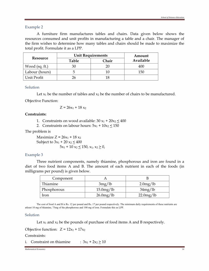
A furniture firm manufactures tables and chairs. Data given below shows the resources consumed and unit profits in manufacturing a table and a chair. The manager of the firm wishes to determine how many tables and chairs should be made to maximize the total profit. Formulate it as a LPP.
Resource Unit Requirements Amount
Available Table Chair Wood (sq. ft.) 30 20 400 Labour (hours) 5 10 150 Unit Profit 26 18
Solution
Let x1 be the number of tables and x2 be the number of chairs to be manufactured.
Objective Function:
Z = 26x1 + 18 x2
Constraints:
1. Constraints on wood available: 30 x1 + 20x2 < 400 2. Constraints on labour hours: 5x1 + 10x2 < 150
The problem is Maximize Z = 26x1 + 18 x2 Subject to 3x1 + 20 x2 < 400 5x1 + 10 x2 < 150, x1, x2 > 0,
Example 3
Three nutrient components, namely thiamine, phosphorous and iron are found in a diet of two food items A and B. The amount of each nutrient in each of the foods (in milligrams per pound) is given below.
Component A B Thiamine 3mg/lb 2.0mg/lb Phosphorous 15.0mg/lb 34mg/lb Iron 26.0mg/lb 22.0mg/lb
The cost of food A and B is Rs. 12 per pound and Rs. 17 per pound respectively. The minimum daily requirements of these nutrients are atleast 10 mg of thiamine, 75mg of the phosphorous and 100 mg of iron. Formulate this as LPP.
Solution
Let x1 and x2 be the pounds of purchase of food items A and B respectively.
Objective function: Z = 12x1 + 17x2 Constraints: i. Constraint on thiamine : 3x1 + 2x2 > 10
School of Distance Education
Mathematical Economics 15
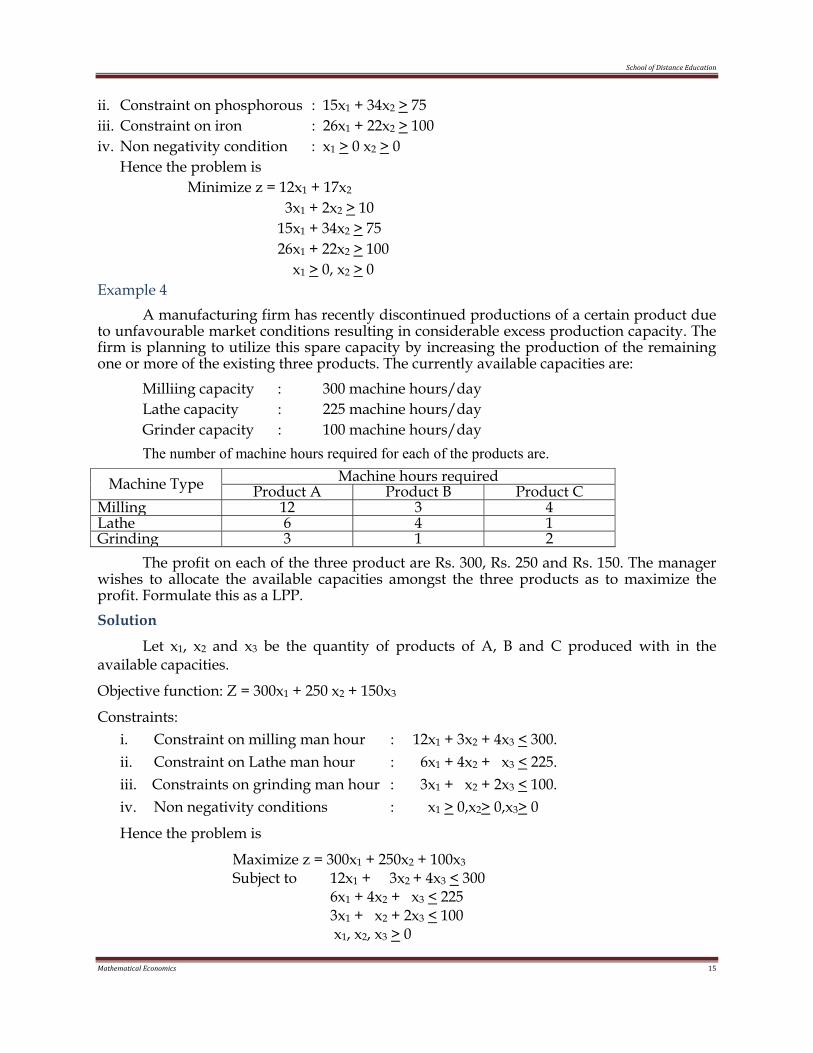
ii. Constraint on phosphorous : 15x1 + 34x2 > 75 iii. Constraint on iron : 26x1 + 22x2 > 100 iv. Non negativity condition : x1 > 0 x2 > 0 Hence the problem is Minimize z = 12x1 + 17x2 3x1 + 2x2 > 10 15x1 + 34x2 > 75 26x1 + 22x2 > 100 x1 > 0, x2 > 0 Example 4 A manufacturing firm has recently discontinued productions of a certain product due to unfavourable market conditions resulting in considerable excess production capacity. The firm is planning to utilize this spare capacity by increasing the production of the remaining one or more of the existing three products. The currently available capacities are: Milliing capacity : 300 machine hours/day Lathe capacity : 225 machine hours/day Grinder capacity : 100 machine hours/day The number of machine hours required for each of the products are.
Machine Type Machine hours required Product A Product B Product C
Milling 12 3 4 Lathe 6 4 1 Grinding 3 1 2 The profit on each of the three product are Rs. 300, Rs. 250 and Rs. 150. The manager wishes to allocate the available capacities amongst the three products as to maximize the profit. Formulate this as a LPP. Solution
Let x1, x2 and x3 be the quantity of products of A, B and C produced with in the available capacities.
Objective function: Z = 300x1 + 250 x2 + 150x3
Constraints: i. Constraint on milling man hour : 12x1 + 3x2 + 4x3 < 300. ii. Constraint on Lathe man hour : 6x1 + 4x2 + x3 < 225. iii. Constraints on grinding man hour : 3x1 + x2 + 2x3 < 100. iv. Non negativity conditions : x1 > 0,x2> 0,x3> 0
Hence the problem is
Maximize z = 300x1 + 250x2 + 100x3
Subject to 12x1 + 3x2 + 4x3 < 300 6x1 + 4x2 + x3 < 225 3x1 + x2 + 2x3 < 100 x1, x2, x3 > 0
School of Distance Education
Mathematical Economics 16
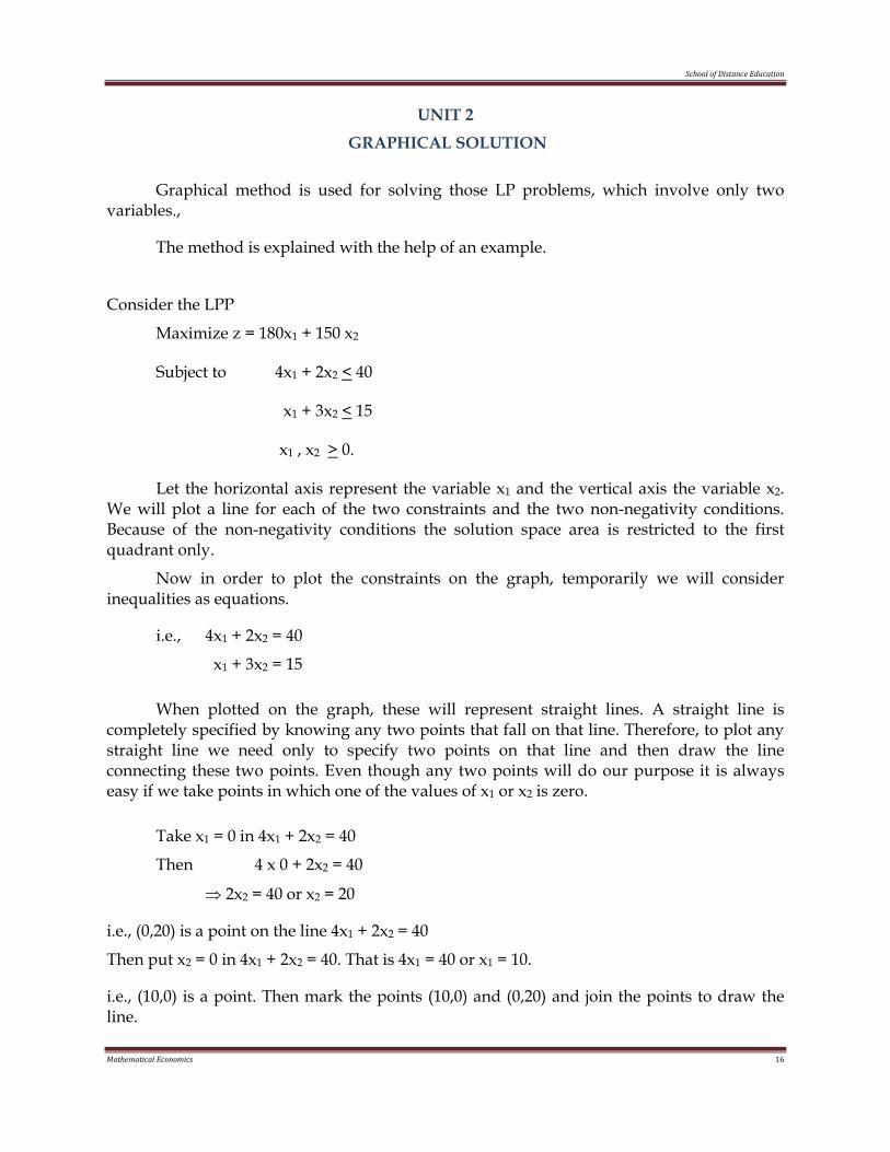
UNIT 2
GRAPHICAL SOLUTION
Graphical method is used for solving those LP problems, which involve only two variables.,
The method is explained with the help of an example.
Consider the LPP
Maximize z = 180x1 + 150 x2
Subject to 4x1 + 2x2 < 40
x1 + 3x2 < 15
x1 , x2 > 0.
Let the horizontal axis represent the variable x1 and the vertical axis the variable x2. We will plot a line for each of the two constraints and the two non-negativity conditions. Because of the non-negativity conditions the solution space area is restricted to the first quadrant only.
Now in order to plot the constraints on the graph, temporarily we will consider inequalities as equations.
i.e., 4x1 + 2x2 = 40
x1 + 3x2 = 15
When plotted on the graph, these will represent straight lines. A straight line is completely specified by knowing any two points that fall on that line. Therefore, to plot any straight line we need only to specify two points on that line and then draw the line connecting these two points. Even though any two points will do our purpose it is always easy if we take points in which one of the values of x1 or x2 is zero.
Take x1 = 0 in 4x1 + 2x2 = 40
Then 4 x 0 + 2x2 = 40
⇒ 2x2 = 40 or x2 = 20
i.e., (0,20) is a point on the line 4x1 + 2x2 = 40
Then put x2 = 0 in 4x1 + 2x2 = 40. That is 4x1 = 40 or x1 = 10.
i.e., (10,0) is a point. Then mark the points (10,0) and (0,20) and join the points to draw the line.
School of Distance Education
Mathematical Economics 17
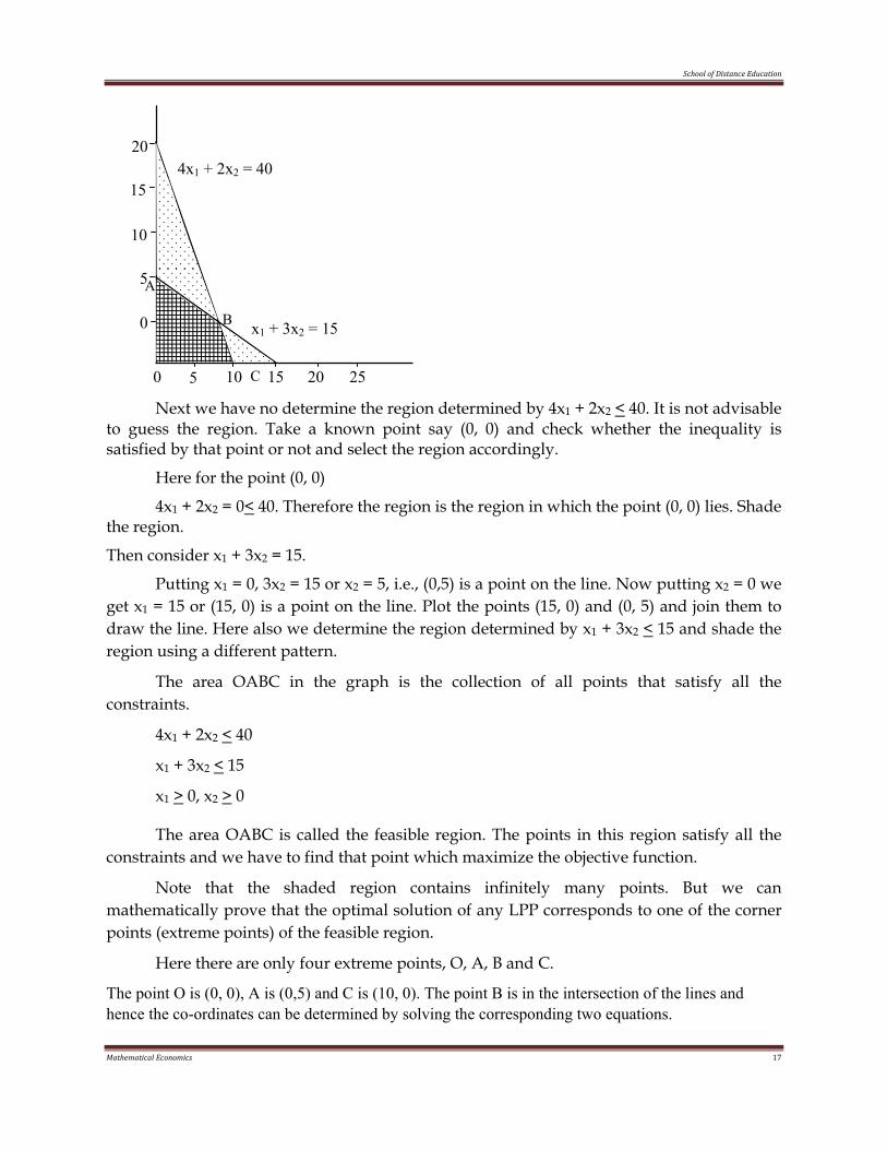
Next we have no determine the region determined by 4x1 + 2x2 < 40. It is not advisable to guess the region. Take a known point say (0, 0) and check whether the inequality is satisfied by that point or not and select the region accordingly.
Here for the point (0, 0)
4x1 + 2x2 = 0< 40. Therefore the region is the region in which the point (0, 0) lies. Shade the region.
Then consider x1 + 3x2 = 15.
Putting x1 = 0, 3x2 = 15 or x2 = 5, i.e., (0,5) is a point on the line. Now putting x2 = 0 we get x1 = 15 or (15, 0) is a point on the line. Plot the points (15, 0) and (0, 5) and join them to draw the line. Here also we determine the region determined by x1 + 3x2 < 15 and shade the region using a different pattern.
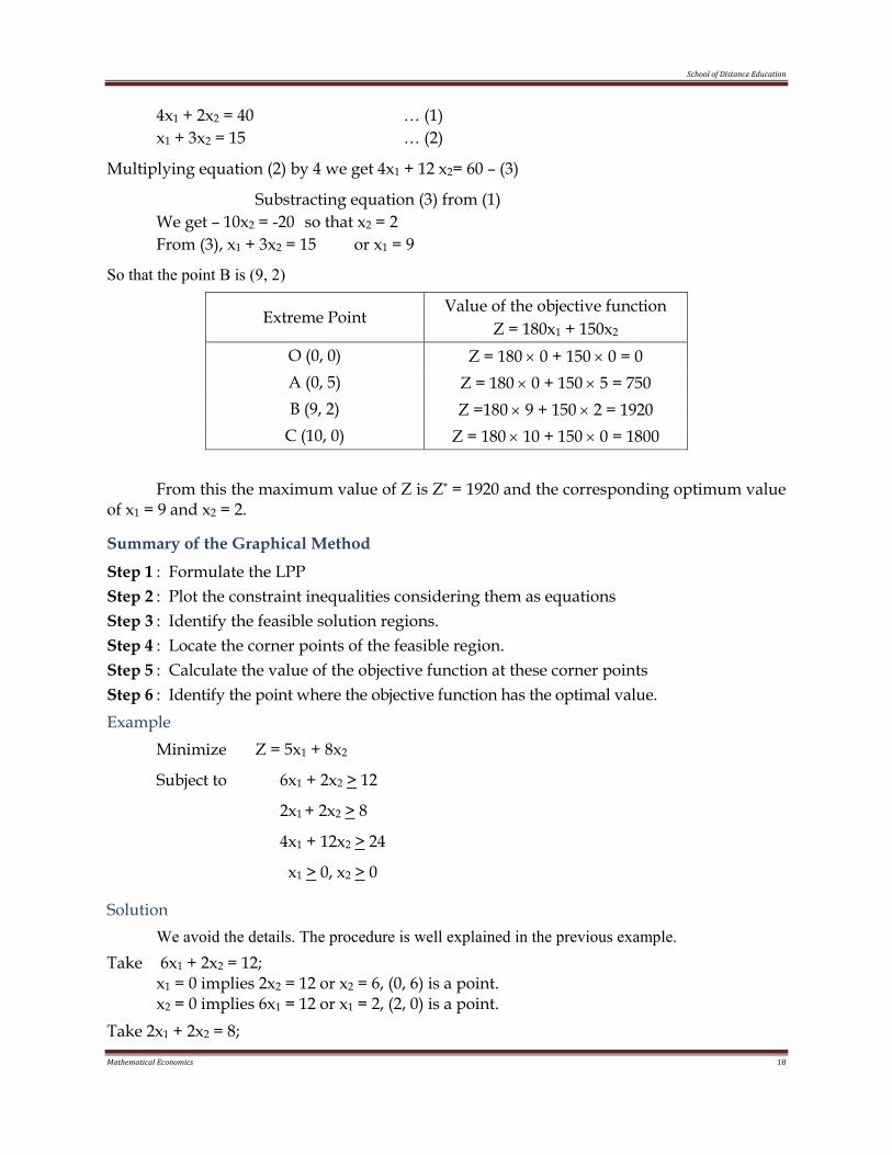
The area OABC in the graph is the collection of all points that satisfy all the constraints.
4x1 + 2x2 < 40
x1 + 3x2 < 15
x1 > 0, x2 > 0
The area OABC is called the feasible region. The points in this region satisfy all the constraints and we have to find that point which maximize the objective function.
Note that the shaded region contains infinitely many points. But we can mathematically prove that the optimal solution of any LPP corresponds to one of the corner points (extreme points) of the feasible region.
Here there are only four extreme points, O, A, B and C.
The point O is (0, 0), A is (0,5) and C is (10, 0). The point B is in the intersection of the lines and hence the co-ordinates can be determined by solving the corresponding two equations.
0 5 10 15 20 25
0
5
10
15
20 4x1 + 2x2 = 40
A
C
B x1 + 3x2 = 15
School of Distance Education
Mathematical Economics 18
4x1 + 2x2 = 40 … (1) x1 + 3x2 = 15 … (2)
Multiplying equation (2) by 4 we get 4x1 + 12 x2= 60 – (3)
Substracting equation (3) from (1) We get – 10x2 = -20 so that x2 = 2 From (3), x1 + 3x2 = 15 or x1 = 9
So that the point B is (9, 2)
Extreme Point Value of the objective function
Z = 180x1 + 150x2 O (0, 0) Z = 180 × 0 + 150 × 0 = 0 A (0, 5) Z = 180 × 0 + 150 × 5 = 750 B (9, 2) Z =180 × 9 + 150 × 2 = 1920
C (10, 0) Z = 180 × 10 + 150 × 0 = 1800
From this the maximum value of Z is Z* = 1920 and the corresponding optimum value of x1 = 9 and x2 = 2.
Summary of the Graphical Method
Step 1 : Formulate the LPP Step 2 : Plot the constraint inequalities considering them as equations Step 3 : Identify the feasible solution regions. Step 4 : Locate the corner points of the feasible region. Step 5 : Calculate the value of the objective function at these corner points Step 6 : Identify the point where the objective function has the optimal value. Example Minimize Z = 5x1 + 8x2
Subject to 6x1 + 2x2 > 12
2x1 + 2x2 > 8
4x1 + 12x2 > 24
x1 > 0, x2 > 0
Solution We avoid the details. The procedure is well explained in the previous example. Take 6x1 + 2x2 = 12; x1 = 0 implies 2x2 = 12 or x2 = 6, (0, 6) is a point. x2 = 0 implies 6x1 = 12 or x1 = 2, (2, 0) is a point. Take 2x1 + 2x2 = 8;
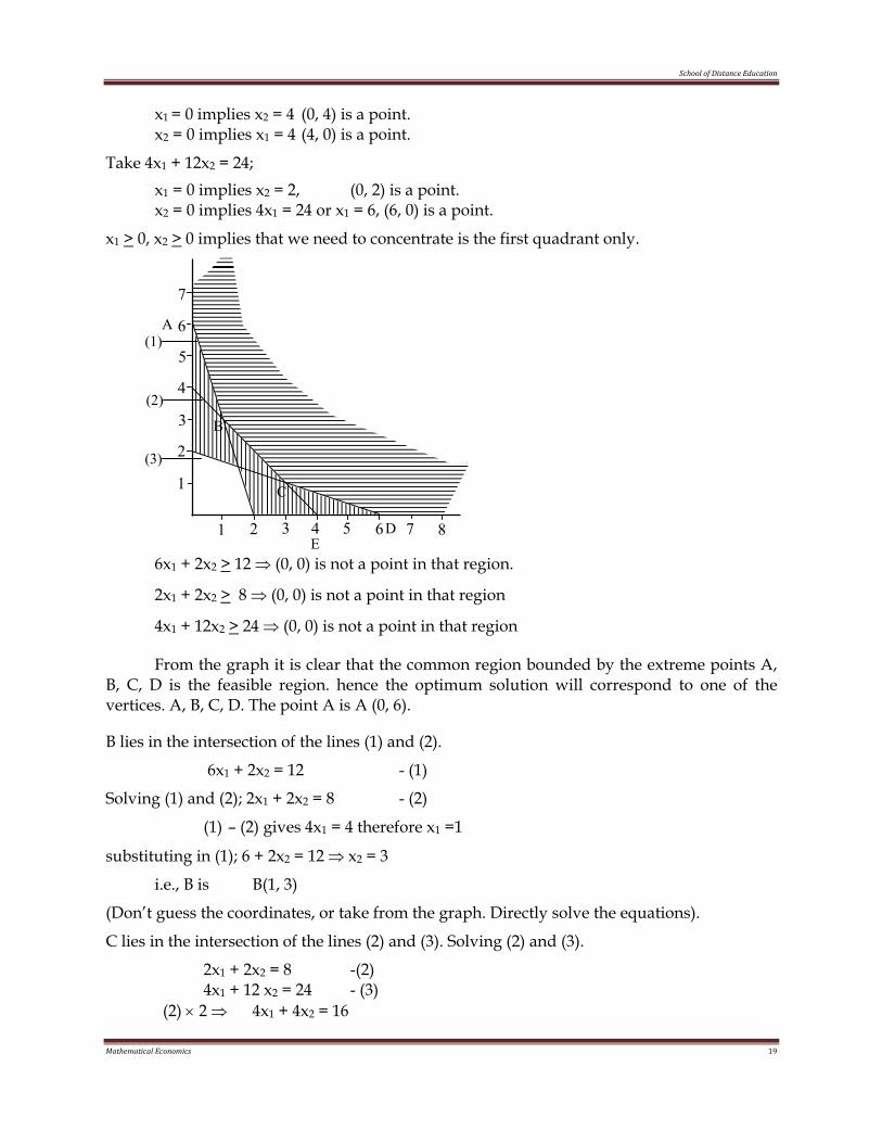
School of Distance Education
Mathematical Economics 19
x1 = 0 implies x2 = 4 (0, 4) is a point. x2 = 0 implies x1 = 4 (4, 0) is a point.
Take 4x1 + 12x2 = 24; x1 = 0 implies x2 = 2, (0, 2) is a point. x2 = 0 implies 4x1 = 24 or x1 = 6, (6, 0) is a point.
x1 > 0, x2 > 0 implies that we need to concentrate is the first quadrant only.
6x1 + 2x2 > 12 ⇒ (0, 0) is not a point in that region.
2x1 + 2x2 > 8 ⇒ (0, 0) is not a point in that region
4x1 + 12x2 > 24 ⇒ (0, 0) is not a point in that region
From the graph it is clear that the common region bounded by the extreme points A, B, C, D is the feasible region. hence the optimum solution will correspond to one of the vertices. A, B, C, D. The point A is A (0, 6).
B lies in the intersection of the lines (1) and (2).
6x1 + 2x2 = 12 - (1)
Solving (1) and (2); 2x1 + 2x2 = 8 - (2)
(1) – (2) gives 4x1 = 4 therefore x1 =1
substituting in (1); 6 + 2x2 = 12 ⇒ x2 = 3
i.e., B is B(1, 3)
(Don’t guess the coordinates, or take from the graph. Directly solve the equations).
C lies in the intersection of the lines (2) and (3). Solving (2) and (3).
2x1 + 2x2 = 8 -(2) 4x1 + 12 x2 = 24 - (3)
(2) × 2 ⇒ 4x1 + 4x2 = 16
4
A
B
D
(1)
7
2
1 2 3 4 5
1
5
6
6
3
7
E
C
8
(2)
(3)
School of Distance Education
Mathematical Economics 20
(3) – (4) ⇒ 8x2 = 8 ⇒ x2 = 1 Putting in (2) ⇒ 2x1 + 2 = 8 ⇒ x1 = 3 i.e., C is (3, 1).
Extreme Point Value of the objective function Z = 5x1 + 8x2
A (0, 6) Z = 5 × 0 + 8 × 6 = 48 B (1, 3) Z = 5 × 1 + 8 × 3 = 29 C (3, 1) Z =5 × 3 + 8 = 23* D (6, 0) Z = 5 × 6 + 0 = 30
The minimum value of Z is Z* = 23 and the optimum solution is *
1x =3,
*
2x =1.
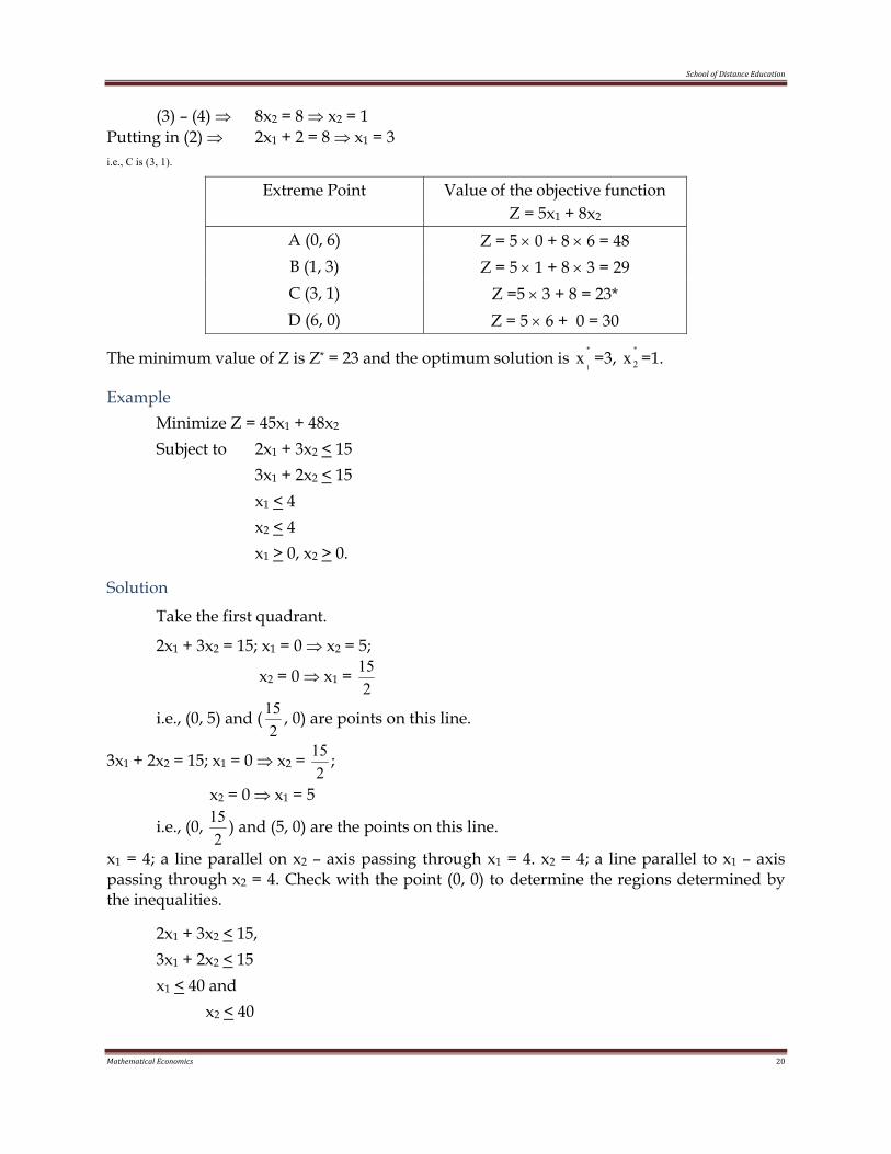
Example Minimize Z = 45x1 + 48x2 Subject to 2x1 + 3x2 < 15 3x1 + 2x2 < 15 x1 < 4 x2 < 4 x1 > 0, x2 > 0.
Solution
Take the first quadrant.
2x1 + 3x2 = 15; x1 = 0 ⇒ x2 = 5;
x2 = 0 ⇒ x1 = 2
15
i.e., (0, 5) and (2
15 , 0) are points on this line.
3x1 + 2x2 = 15; x1 = 0 ⇒ x2 = 2
15 ;
x2 = 0 ⇒ x1 = 5
i.e., (0, 2
15 ) and (5, 0) are the points on this line.
x1 = 4; a line parallel on x2 – axis passing through x1 = 4. x2 = 4; a line parallel to x1 – axis passing through x2 = 4. Check with the point (0, 0) to determine the regions determined by the inequalities.
2x1 + 3x2 < 15, 3x1 + 2x2 < 15 x1 < 40 and x2 < 40
School of Distance Education
Mathematical Economics 21
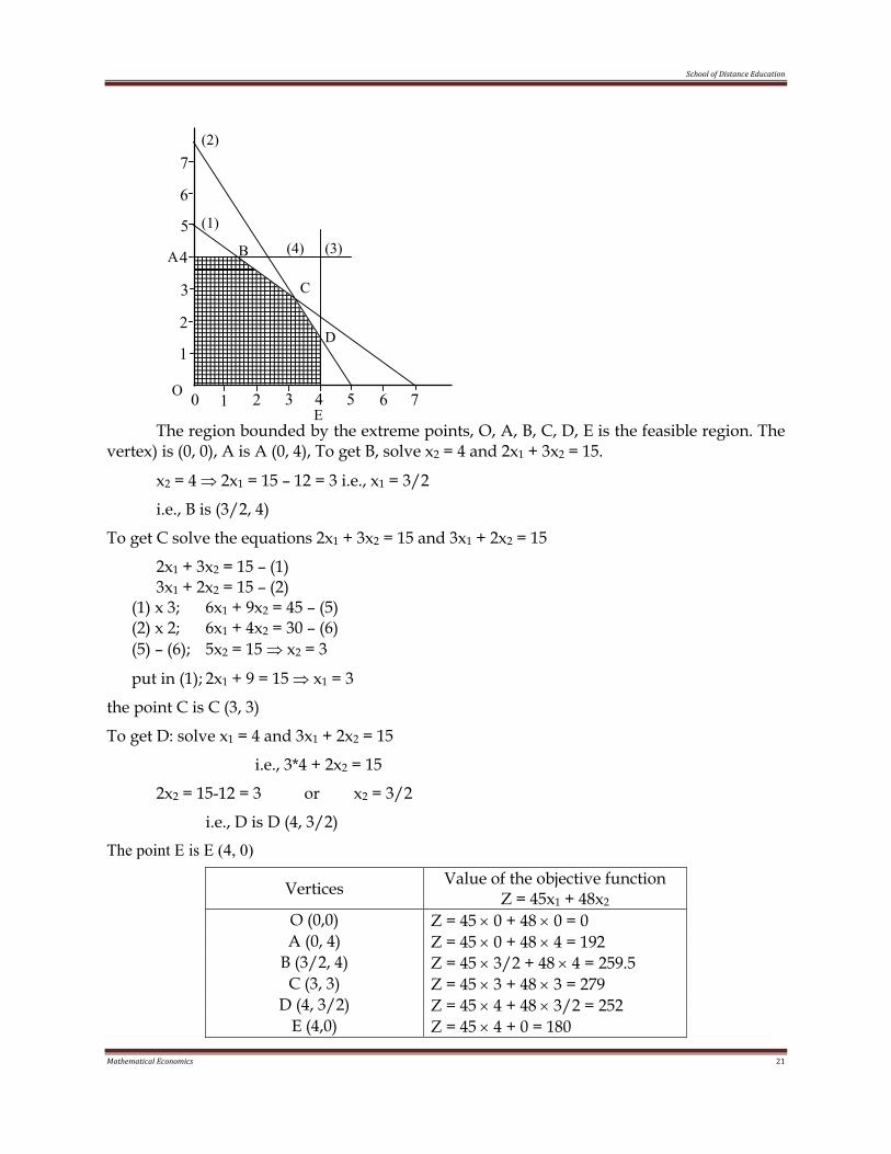
The region bounded by the extreme points, O, A, B, C, D, E is the feasible region. The vertex) is (0, 0), A is A (0, 4), To get B, solve x2 = 4 and 2x1 + 3x2 = 15.
x2 = 4 ⇒ 2x1 = 15 – 12 = 3 i.e., x1 = 3/2
i.e., B is (3/2, 4)
To get C solve the equations 2x1 + 3x2 = 15 and 3x1 + 2x2 = 15
2x1 + 3x2 = 15 – (1) 3x1 + 2x2 = 15 – (2)
(1) x 3; 6x1 + 9x2 = 45 – (5) (2) x 2; 6x1 + 4x2 = 30 – (6) (5) – (6); 5x2 = 15 ⇒ x2 = 3
put in (1); 2x1 + 9 = 15 ⇒ x1 = 3
the point C is C (3, 3)
To get D: solve x1 = 4 and 3x1 + 2x2 = 15
i.e., 3*4 + 2x2 = 15
2x2 = 15-12 = 3 or x2 = 3/2
i.e., D is D (4, 3/2)
The point E is E (4, 0)
Vertices Value of the objective function Z = 45x1 + 48x2
O (0,0) Z = 45 × 0 + 48 × 0 = 0 A (0, 4) Z = 45 × 0 + 48 × 4 = 192
B (3/2, 4) Z = 45 × 3/2 + 48 × 4 = 259.5 C (3, 3) Z = 45 × 3 + 48 × 3 = 279
D (4, 3/2) Z = 45 × 4 + 48 × 3/2 = 252 E (4,0) Z = 45 × 4 + 0 = 180
4 A
0 1 2 3 4 5
1
2
5
6
(3)
C
6 7
3
7
B
D
(4)
(2)
(1)
O E
School of Distance Education
Mathematical Economics 22
Maximum of Z is Z* = 279
and the optimum solution is *1x = 3, *
2x = 3.
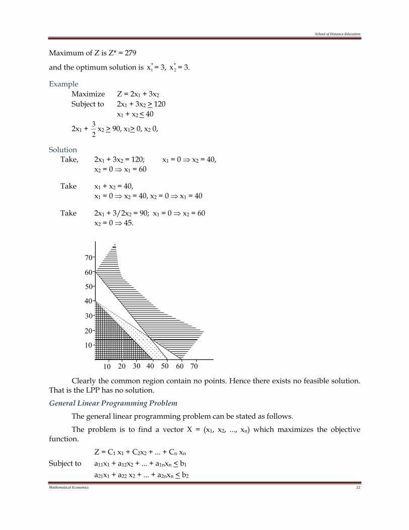
Example Maximize Z = 2x1 + 3x2 Subject to 2x1 + 3x2 > 120 x1 + x2 < 40
2x1 + 23 x2 > 90, x1> 0, x2 0,
Solution Take, 2x1 + 3x2 = 120; x1 = 0 ⇒ x2 = 40, x2 = 0 ⇒ x1 = 60
Take x1 + x2 = 40, x1 = 0 ⇒ x2 = 40, x2 = 0 ⇒ x1 = 40
Take 2x1 + 3/2x2 = 90; x1 = 0 ⇒ x2 = 60 x2 = 0 ⇒ 45.
Clearly the common region contain no points. Hence there exists no feasible solution. That is the LPP has no solution.
General Linear Programming Problem
The general linear programming problem can be stated as follows.
The problem is to find a vector X = (x1, x2, ..., xn) which maximizes the objective function.
Z = C1 x1 + C2x2 + ... + Cn xn Subject to a11x1 + a12x2 + ... + a1nxn < b1 a21x1 + a22 x2 + ... + a2nxn < b2
40
10 20 30 40 50
10
20
50
60
60 70
30
70
School of Distance Education
Mathematical Economics 23
M am1x1 + am2 x2 + ... + amn xn < bm and xj > 0; j = 1, 2, ..., n.
where aij, bi and cj are known constants and m < n.
Applications of LP
Linear programming is the most widely used technique of decision-making in business, industry and in various other fields.
1. Production management: Linear programming techniques can be used in production management to determine the optimal product mix to make the optimum use of available resources.
2. Marketing management: Linear programming helps in analyzing the audience coverage of an advertising campaign based on the available advertising media and budget. LP is also used to determine the optimal distribution of the products from various factories to different stores in a minimum cost. This is called transportation problem. Also it is useful to a travelling salesman to determine the shortest route for his tour. This is known as travelling salesman problem.
3. Personnel management: LP techniques are useful to analyze the problems related to selections and training of employees. It is also used to determine the optimum assignment of works to workers so as to complete the work in a minimum cost. This is known as assignment problem.
The technique can be used to determine the minimum number of employees need to work in various shifts for optimum production.
4. Financial management: LP techniques can be used as a powerful tool to select proper investment schemes from the various available ones.
Merits and Limitations of L/P
Merits
Linear programming can be used to solve allocation type problems. Usually their solution is difficult due to the fact that there is a possibility of infinitely many solutions. Using LP techniques we can determine the optimal solution in a very efficient way. It also provides additional information concerning the value of the resources to be allocated. It allows modification of its mathematical solution.
Linear programming improve the quality of decisions. It makes decisions more objective than subjective. Linear programming helps in highlighting the bottlenecks in the production processes. Linear programming helps in attaining optimum use of production factors. It also indicates the significance and utility of these factors more effectively.
School of Distance Education
Mathematical Economics 24
Limitations
The linear programming problem assumes the linearity of objective function and constraints. But in most of the real life situations the objective function and constraints are not linearly related to the variables. To solve such problems we have to use non-linear programming techniques. Again if we want the solution in integers, LP Model may not be always useful. We have to use integer programming techniques in such situations. A major assumption regarding the parameters appearing in the LP model are assumed to be constant through out. But in real-life situations they are not known completely. In some cases they are random variables. In such cases we use stochastic programming techniques.
Another limitation of LP technique is that it does not take into consideration the effect of time and uncertainty. Again in LP models we deal with only one objective where as in real life situations we may come across more than one objective. Where we have two or more objectives to optimize we may use Goal programming techniques.
School of Distance Education
Mathematical Economics 25
UNIT 3
SIMPLEX METHOD
We explain the principle of the simplex method with the help of the two variable linear programming problem by means of the following examples.
Example 1
Maximize 50x1+60x2
Subject to 2x1 + x2 < 300 3x1 + 4x2 < 509 4x1 + 7x2 < 812
x1 and x2 > 0
Solution
We introduce variable x3 > 0, x4 > 0, x5 > 0
So that the constraints become equations as,
2x1 + x2 + x3 = 300 3x1 + 4x2 + x4 = 509 4x1 + 7x2 + x5 = 812
The variables x3, x4, x5 are known as slack variables corresponding to the three constraints. The system of equations has five variables (including the slack variables) and three equations.
Basic Solution
In the system of equations as presented above we may equate any two variables to zero. The system then consists of three equations with three variables. If this system of three equations with three variables is solvable such a solution is known as a basic solution.
In the example considered above suppose we take x1 = 0, x2 = 0. The solution of the system with remaining three variables is x3 = 300, x4 = 509, x5 = 812. This is a basic solution of the system. The variables x3, x4 and x5 are known as basic variables while the variables x1, x2 are known as non basic variables (variables which are equated to zero).
Since there are three equations and five variables the two non basic variables can be chosen in 5C2 = 10 ways. Thus, the maximum number of basic solutions is 10, for in some cases the three variable three equation problem may not be solvable.
In the general case, if the number of constraints of the linear programming problem is m and the number of variables (including the slack variables) is n then there are at most nCn–m = nCm basic solutions.
School of Distance Education
Mathematical Economics 26
Basic Feasible Solution
A basic solution of a linear programming problem is a basic feasible solution if it is feasible, i.e., all the variables are non negative. The solution x3 = 300, x4 = 509, x5 = 812 is a basic feasible solution of the problem. Again, if the number of constraints is m and the number of variables (including the slack variables) is n, the maximum number of basic feasible solution is nCn–m = nCm.
The following result (Hadley, 1069) will help you to identify the extreme points of the convex set of feasible solutions analytically.
Every basic feasible solution of the problem is an extreme point of the convex set of feasible solutions and every extreme point is a basic feasible solution of the set of constraints.
When several variables are present in a linear programming problem it is not possible to identify the extreme points geometrically. But we can identify them through the basic feasible solutions. Since one of the basic feasible solutions will maximize or minimize the objective function, we can carry out this search starting from one basic feasible solution to another. The simplex method provides a systematic search so that the objective function increases (in the case of maximization) progressively until the basic feasible solution has been identified where the objective function is maximized. The computational aspect of the simplex method is presented in the next section.
COMPUTATIONAL ASPECT OF SIMPLEX METHOD
We again consider the linear programming problem
Maximize 50x1+60x2
Subject to 2x1 + x2 + x3 = 300
3x1 + 4x2 + x4 = 509
4x1 + 7x2 + x5 = 812
x1 > 0, x2 > 0, x3 > 0, x4 > 0, x5 > 0
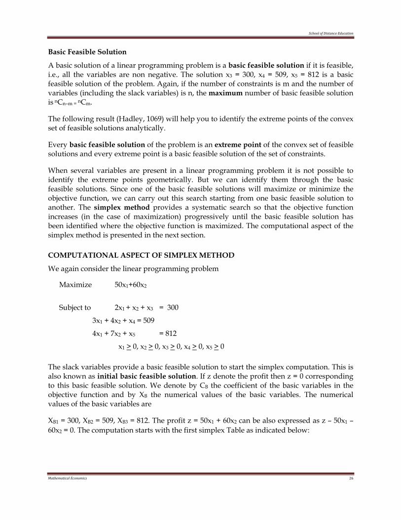
The slack variables provide a basic feasible solution to start the simplex computation. This is also known as initial basic feasible solution. If z denote the profit then z = 0 corresponding to this basic feasible solution. We denote by CB the coefficient of the basic variables in the objective function and by XB the numerical values of the basic variables. The numerical values of the basic variables are
XB1 = 300, XB2 = 509, XB3 = 812. The profit z = 50x1 + 60x2 can be also expressed as z – 50x1 – 60x2 = 0. The computation starts with the first simplex Table as indicated below:
School of Distance Education
Mathematical Economics 27
Table 1
CB Basic Variables
Cj
XB
50 60 0 0 0
0 x3 300 2 1 1 0 0 0 x4 509 3 4 0 1 0 0 x5 812 4 7 0 0 1 z -50 -60 0 0 0
The coefficients of the basic variables in the objective function are CB1=CB2=CB3= 0. The topmost row of Table 1 indicates the coefficient of the variables x1, x2, x3, x4 and x5 in the objective function respectively. The column under x1 presents the coefficient of x1 in the three equations. The remaining columns have also been formed in a similar manner.
On examining the profit equation z = 50x1 + 60x2 you may observe that if either x1 or x2 which is currently non basic is included as a basic variable the profit will increase. Since the coefficient of x2 is numerically higher we choose x2 to be included as a basic variable in the next iteration. An equivalent criterion of choosing a new basic variable can be obtained from the last row of Table 1 (corresponding to z). Since the entry corresponding x2 is smaller between the two negative values x2 will be included as a basic variable in the next iteration. However with three constraints there can only be three basic variables. Thus by making x2 a basic variable one of the existing basic variables will become non basic. You may identify this variable using the following line of argument.
From the first equation
2x1 + x3 = 300 – x2
But x1 = 0. Hence, in order that x3 > 0
300 – x2 > 0 i.e., x2 < 300
Similar computation from the second and the third equation lead to
x2 < 4
509 , x2 < 7
812 = 116
Thus x2 = Min ⎟⎠⎞
⎜⎝⎛
7812,
4509,
1300 = 116
If x2 = 116, from the third equation you may observe that
7x2 + x5 = 812 i.e., x5 = 0
Thus the variable x5 becomes non basic in the next iteration. The revised values of the other two basic variable are
x3 = 300 – x2 = 184
x4 = 509 – 4 ×116 = 45
Referring back to Table 1, we obtain elements of the next Table (Table 2) using the following rules:
School of Distance Education
Mathematical Economics 28
1) In the z row we locate the quantities which are negative. If all the quantities are positive, the inclusion of any non basic variable will not increase the value of the objective function. Hence the present solution maximizes the objective function. If there are more than one negative values we choose the variable as a basic variable corresponding to which the z value is least as this is likely to increase the profit most.
2) Let xj be the incoming basic variable and the corresponding elements of the jth column be denoted by yij, y2j and y3j. If the present values of basic variables are xB1, xB2 and xB3 respectively, then we compute
Min ⎥⎥⎦
⎤
⎢⎢⎣
⎡
j3
3B
j2
2B
j1
1B
yx,
yx,
yx
for y1j > 0, y2j > 0, y3j> 0. You may note that if any yij<0, this need not be included in
the comparison. If the minimum occurs corresponding to rj
Br
yx then the rth basic
variable will become non basic in the next iteration.
3) Table 2 is computed from Table 1 using the following rules.
a) The revised basic variables are x3, x4 and x2. Accordingly, we make CB1=0, CB2 = 0 and CB3 = 60
b) As x2 is the incoming basic variable we make the coefficient of x2 one by dividing each element of row 3 by 7. Thus the numerical value of the element
corresponding to x1 is 74 , corresponding to x5 is
71 in Table 2.
c) The incoming basic variable should appear only in the third row. So we multiply the third row of Table 2 by 1 and subtract it from the first row of Table 1 element by element. Thus the element corresponding to x2 in the first row of Table 2 is zero. The element corresponding to x1 is
2 – 1 × 7
1074=
the element corresponding to x5 is
0 –1 × 71
71
−=
In this way we obtain the elements of the first and the second row in Table 2. The numerical values of the basic variables in Table 2 can also be computed in a similar manner.
Let CB1, CB2, CB3 be the coefficients of the basic variables in the objective function. For example in Table 2 CB1 = 0, CB2 = 0, CB3= 60. Suppose corresponding to a variable j, the quantity zj is defined as zj = CB1, Y1 + CB2, Y2j + CB3 Y3j. Then the final row (z-row) can also be expressed as zj – Cj. For example
z1 – c1 = 7
10 × 0 + 75 × 0 + 60 ×
74 – 50= –
7100
School of Distance Education
Mathematical Economics 29
z5 – c5 = – 71 × 0 –
74 × 0 +
71 × 60 – 0 =
760
1) We now apply rule 1 to Table 2. The only negative zj – cj is z1-c1 = – 7
100
Hence x1 should be made a basic variable at the next iteration.
2) We compute the minimum of the ratios
Min ⎥⎥⎥
⎦
⎤
⎢⎢⎢
⎣
⎡
74
116
7545,
710184
= Min ⎥⎦⎤
⎢⎣⎡ 203,63,
5644 = 63.
Since this minimum occurs corresponding to x4, it becomes a non basic variable in next iteration.
3) Table 3 is computed from Table 2 using the rules (a), (b) and (c) as described before.
Table 2
CB Basic Variables
Cj
XB
50 x1
60 x2
0 x3
0 x4
0 x5
0 x3 184 7
10 0 1 0 –71
0 x4 45 75 0 0 1 –
74
60 x2 116 74 1 0 0
71
zj – cj 7100− 0 0 0
760
Table 3
CB Basic Variables
Cj
XB
50 x1
60 x2
0 x3
0 x4
0 x5
0 x3 94 0 0 1 –2 1
50 x1 63 1 0 0 57 – 4/5
60 x2 80 0 1 0 –4/5 3/5
zj – cj 0 0 0 22 – 4
1) z5 – c5 < 0. Hence x5 should be made a basic variable in the next iteration. 2) We compute the minimum of the ratios
School of Distance Education
Mathematical Economics 30
Min ⎥⎦⎤
⎢⎣⎡
5/380,
194 = 94
Note that since y25<0, the corresponding ratio is not taken for comparison. The variable x3 becomes non basic at the next iteration.
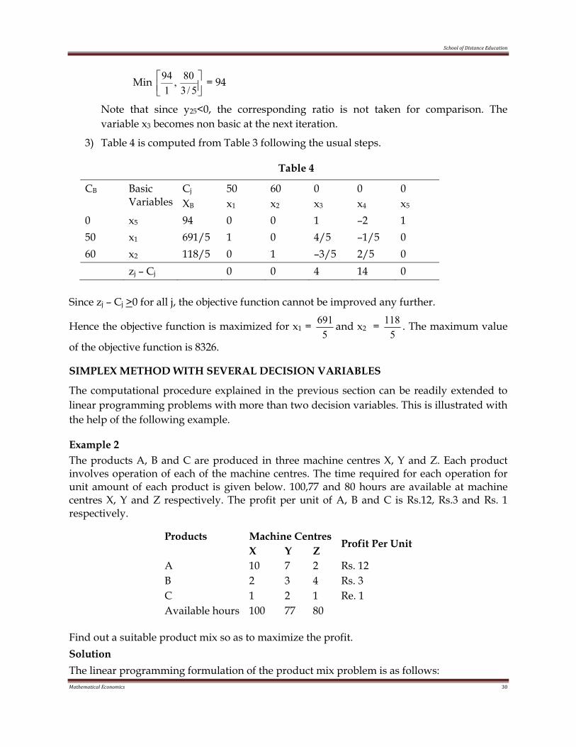
3) Table 4 is computed from Table 3 following the usual steps.
Table 4
CB Basic Variables
Cj
XB
50 x1
60 x2
0 x3
0 x4
0 x5
0 x5 94 0 0 1 –2 1 50 x1 691/5 1 0 4/5 –1/5 0 60 x2 118/5 0 1 –3/5 2/5 0 zj – Cj 0 0 4 14 0
Since zj – Cj >0 for all j, the objective function cannot be improved any further.
Hence the objective function is maximized for x1 = 5
691 and x2 = 5
118 . The maximum value
of the objective function is 8326.
SIMPLEX METHOD WITH SEVERAL DECISION VARIABLES
The computational procedure explained in the previous section can be readily extended to linear programming problems with more than two decision variables. This is illustrated with the help of the following example.
Example 2 The products A, B and C are produced in three machine centres X, Y and Z. Each product involves operation of each of the machine centres. The time required for each operation for unit amount of each product is given below. 100,77 and 80 hours are available at machine centres X, Y and Z respectively. The profit per unit of A, B and C is Rs.12, Rs.3 and Rs. 1 respectively.
Products Machine Centres Profit Per Unit
X Y Z A 10 7 2 Rs. 12 B 2 3 4 Rs. 3 C 1 2 1 Re. 1 Available hours 100 77 80
Find out a suitable product mix so as to maximize the profit. Solution The linear programming formulation of the product mix problem is as follows:
School of Distance Education
Mathematical Economics 31
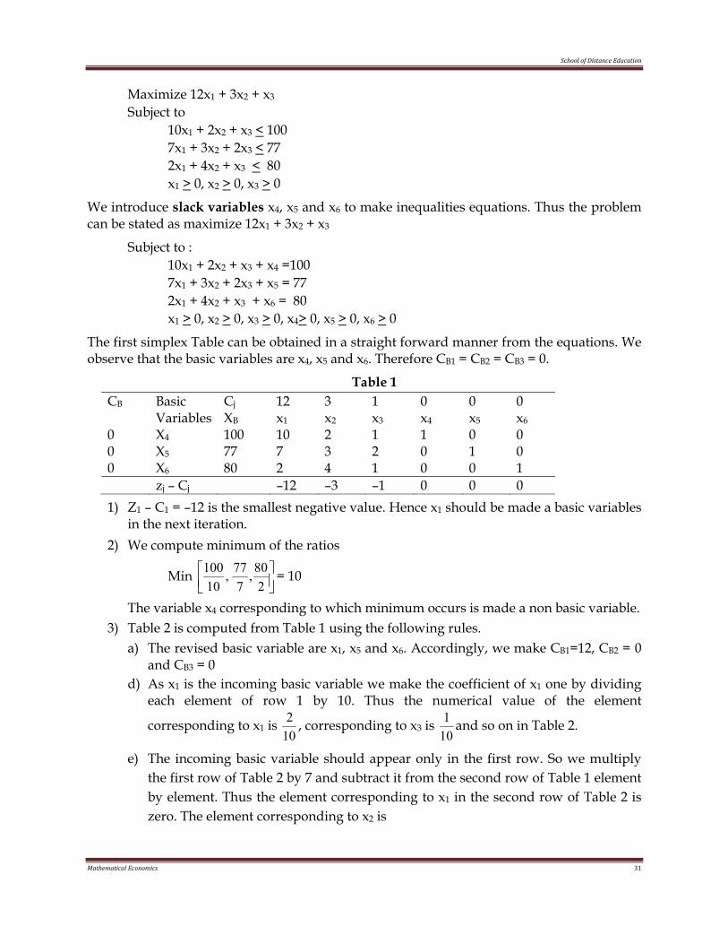
Maximize 12x1 + 3x2 + x3
Subject to 10x1 + 2x2 + x3 < 100
7x1 + 3x2 + 2x3 < 77 2x1 + 4x2 + x3 < 80 x1 > 0, x2 > 0, x3 > 0
We introduce slack variables x4, x5 and x6 to make inequalities equations. Thus the problem can be stated as maximize 12x1 + 3x2 + x3
Subject to : 10x1 + 2x2 + x3 + x4 =100
7x1 + 3x2 + 2x3 + x5 = 77 2x1 + 4x2 + x3 + x6 = 80 x1 > 0, x2 > 0, x3 > 0, x4> 0, x5 > 0, x6 > 0
The first simplex Table can be obtained in a straight forward manner from the equations. We observe that the basic variables are x4, x5 and x6. Therefore CB1 = CB2 = CB3 = 0.
Table 1 CB Basic
Variables Cj
XB
12 x1
3 x2
1 x3
0 x4
0 x5
0 x6
0 X4 100 10 2 1 1 0 0 0 X5 77 7 3 2 0 1 0 0 X6 80 2 4 1 0 0 1 zj – Cj –12 –3 –1 0 0 0 1) Z1 – C1 = –12 is the smallest negative value. Hence x1 should be made a basic variables
in the next iteration. 2) We compute minimum of the ratios
Min ⎥⎦⎤
⎢⎣⎡
280,
777,
10100 = 10
The variable x4 corresponding to which minimum occurs is made a non basic variable. 3) Table 2 is computed from Table 1 using the following rules.
a) The revised basic variable are x1, x5 and x6. Accordingly, we make CB1=12, CB2 = 0 and CB3 = 0
d) As x1 is the incoming basic variable we make the coefficient of x1 one by dividing each element of row 1 by 10. Thus the numerical value of the element
corresponding to x1 is 102 , corresponding to x3 is
101 and so on in Table 2.
e) The incoming basic variable should appear only in the first row. So we multiply the first row of Table 2 by 7 and subtract it from the second row of Table 1 element by element. Thus the element corresponding to x1 in the second row of Table 2 is zero. The element corresponding to x2 is
School of Distance Education
Mathematical Economics 32
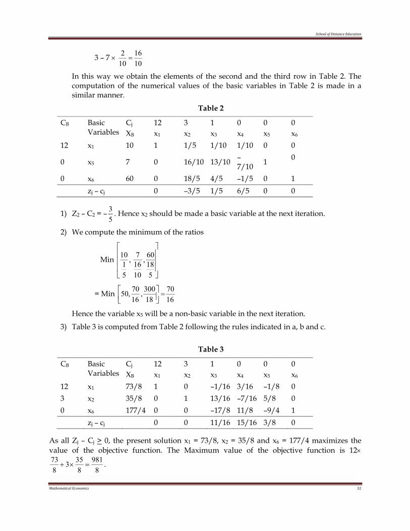
3 – 7 × 10¹⁶
102=
In this way we obtain the elements of the second and the third row in Table 2. The computation of the numerical values of the basic variables in Table 2 is made in a similar manner.
Table 2
CB Basic Variables
Cj
XB
12 x1
3 x2
1 x3
0 x4
0 x5
0 x6
12 x1 10 1 1/5 1/10 1/10 0 0
0 x5 7 0 16/10 13/10 –7/10 1 0
0 x6 60 0 18/5 4/5 –1/5 0 1 zj – cj 0 –3/5 1/5 6/5 0 0
1) Z2 – C2 = –53 . Hence x2 should be made a basic variable at the next iteration.
2) We compute the minimum of the ratios
Min ⎥⎥⎥
⎦
⎤
⎢⎢⎢
⎣
⎡
51860,
10167,
51
10
= Min 1670
18300,
1670,50 =⎥⎦
⎤⎢⎣⎡
Hence the variable x5 will be a non-basic variable in the next iteration.
3) Table 3 is computed from Table 2 following the rules indicated in a, b and c.
Table 3
CB Basic Variables
Cj
XB
12 x1
3 x2
1 x3
0 x4
0 x5
0 x6
12 x1 73/8 1 0 –1/16 3/16 –1/8 0 3 x2 35/8 0 1 13/16 –7/16 5/8 0 0 x6 177/4 0 0 –17/8 11/8 –9/4 1 zj – cj 0 0 11/16 15/16 3/8 0
As all Zj – Cj > 0, the present solution x1 = 73/8, x2 = 35/8 and x6 = 177/4 maximizes the value of the objective function. The Maximum value of the objective function is 12×
8981
8353
873
=×+ .
School of Distance Education
Mathematical Economics 33
TWO PHASE AND M-METHOD
The simplex method illustrated in the last two sections was applied to linear programming problems with less than or equal to type constraints. As a result we could introduce slack variables which provided an initial basic feasible solution of the problem. Linear programming problems may also be characterized by the presence of both “less than or equal to” type or “greater than or equal to type” constraints. It may also contain some equations. Thus it is not always possible to obtain an initial basic feasible solution using slack variables.
Two methods are available to solve linear programming by simplex method in such cases. These methods will be explained with the help of numerical examples.
Two phase method
We illustrate the two phase method with the help of the following example.
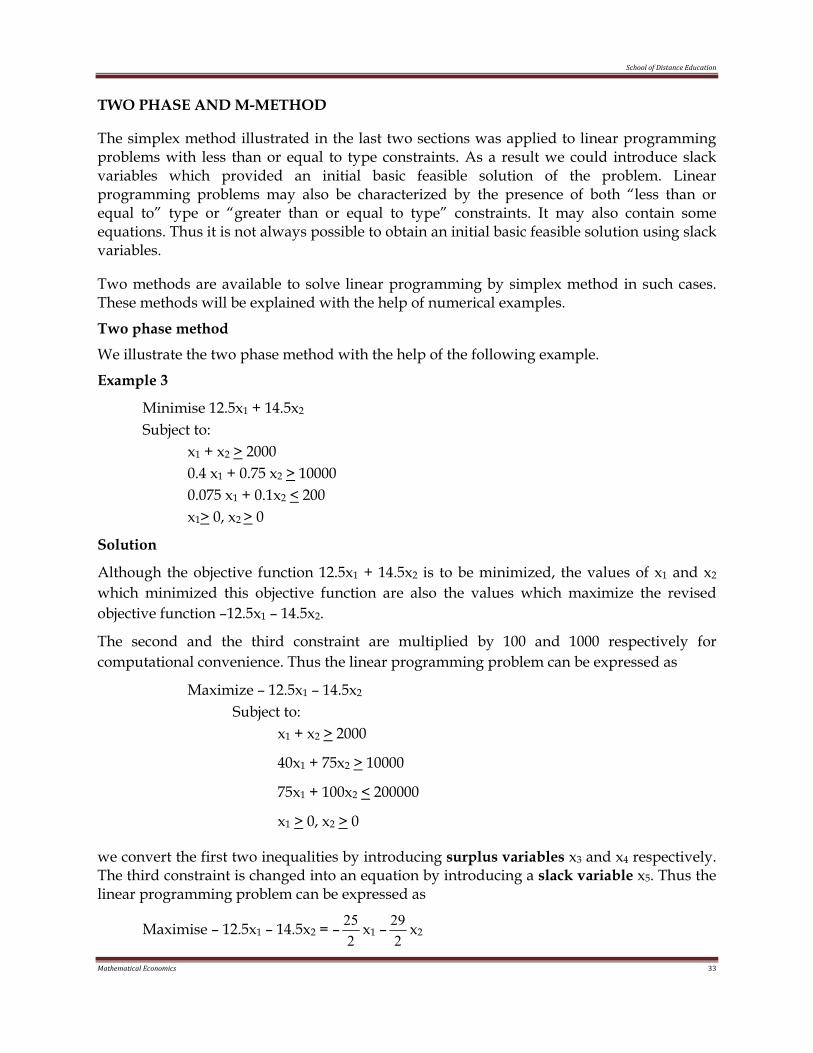
Example 3
Minimise 12.5x1 + 14.5x2 Subject to: x1 + x2 > 2000 0.4 x1 + 0.75 x2 > 10000 0.075 x1 + 0.1x2 < 200 x1> 0, x2 > 0
Solution
Although the objective function 12.5x1 + 14.5x2 is to be minimized, the values of x1 and x2 which minimized this objective function are also the values which maximize the revised objective function –12.5x1 – 14.5x2.
The second and the third constraint are multiplied by 100 and 1000 respectively for computational convenience. Thus the linear programming problem can be expressed as
Maximize – 12.5x1 – 14.5x2 Subject to: x1 + x2 > 2000
40x1 + 75x2 > 10000
75x1 + 100x2 < 200000
x1 > 0, x2 > 0
we convert the first two inequalities by introducing surplus variables x3 and x4 respectively. The third constraint is changed into an equation by introducing a slack variable x5. Thus the linear programming problem can be expressed as
Maximise – 12.5x1 – 14.5x2 = –2
25 x1 –2
29 x2
School of Distance Education
Mathematical Economics 34
Subject to: x1 + x2 – x3 = 2000 40x1 + 75x2 – x4 = 100000 75x1 + 100x2 + x5 = 200000 x1 > 0, x2 > 0, x3 > 0, x3 > 0, x5 > 0
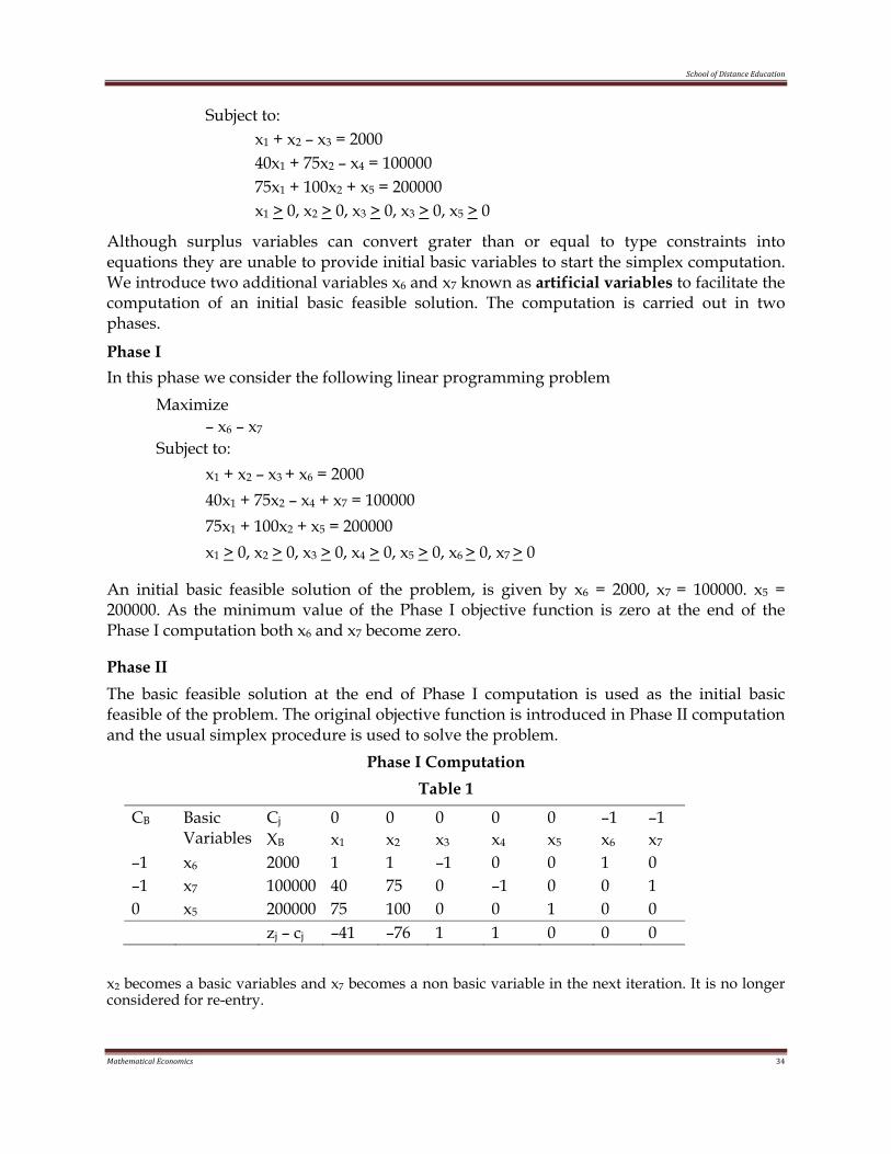
Although surplus variables can convert grater than or equal to type constraints into equations they are unable to provide initial basic variables to start the simplex computation. We introduce two additional variables x6 and x7 known as artificial variables to facilitate the computation of an initial basic feasible solution. The computation is carried out in two phases.
Phase I In this phase we consider the following linear programming problem Maximize – x6 – x7 Subject to: x1 + x2 – x3 + x6 = 2000 40x1 + 75x2 – x4 + x7 = 100000 75x1 + 100x2 + x5 = 200000 x1 > 0, x2 > 0, x3 > 0, x4 > 0, x5 > 0, x6 > 0, x7 > 0
An initial basic feasible solution of the problem, is given by x6 = 2000, x7 = 100000. x5 = 200000. As the minimum value of the Phase I objective function is zero at the end of the Phase I computation both x6 and x7 become zero.
Phase II The basic feasible solution at the end of Phase I computation is used as the initial basic feasible of the problem. The original objective function is introduced in Phase II computation and the usual simplex procedure is used to solve the problem.
Phase I Computation Table 1
CB Basic Variables
Cj
XB
0 x1
0 x2
0 x3
0 x4
0 x5
–1 x6
–1 x7
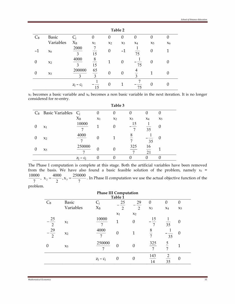
–1 x6 2000 1 1 –1 0 0 1 0 –1 x7 100000 40 75 0 –1 0 0 1 0 x5 200000 75 100 0 0 1 0 0 zj – cj –41 –76 1 1 0 0 0
x2 becomes a basic variables and x7 becomes a non basic variable in the next iteration. It is no longer considered for re-entry.
School of Distance Education
Mathematical Economics 35
Table 2
CB Basic Variables
Cj
XB
0 x1
0 x2
0 x3
0 x4
0 x5
0 x6
–1 x6 32000
157 0 –1
751 0 1
0 x2 34000
158 1 0 –
751 0 0
0 x5 3200000
365 0 0
34 1 0
zj – cj –151 0 1 –
757 0 0
x1 becomes a basic variable and x6 becomes a non basic variable in the next iteration. It is no longer considered for re-entry.
Table 3
CB Basic Variables Cj
XB
0 x1
0 x2
0 x3
0 x4
0 x5
0 x1 710000 1 0 –
715
351 0
0 x2 74000 0 1
78 –
351 0
0 x5 7250000 0 0
7325
2116 1
zj – cj 0 0 0 0 0
The Phase I computation is complete at this stage. Both the artificial variables have been removed from the basis. We have also found a basic feasible solution of the problem, namely x1 =
7250000x,
24000x,
710000
52 == . In Phase II computation we use the actual objective function of the
problem.
Phase III Computation Table 1
CB Basic Variables
Cj
XB 225
−
x1
229
−
x2
0 x3
0 x4
0 x5
225
− x1 710000 1 0 –
715
351 0
229
− x2 74000 0 1
78 –
351 0
0 x5 7250000 0 0
7325
75 1
zj – cj 0 0 14143
352 0
School of Distance Education
Mathematical Economics 36
As all Zj – Cj > 0 the current solution maximizes the revised objective function. Hence the
solution of the problem is given by x1 = 7
10000 = 1428 74 , x2 =
74000 = 571
73 . The minimum
vale of the objective function is 2614276 .
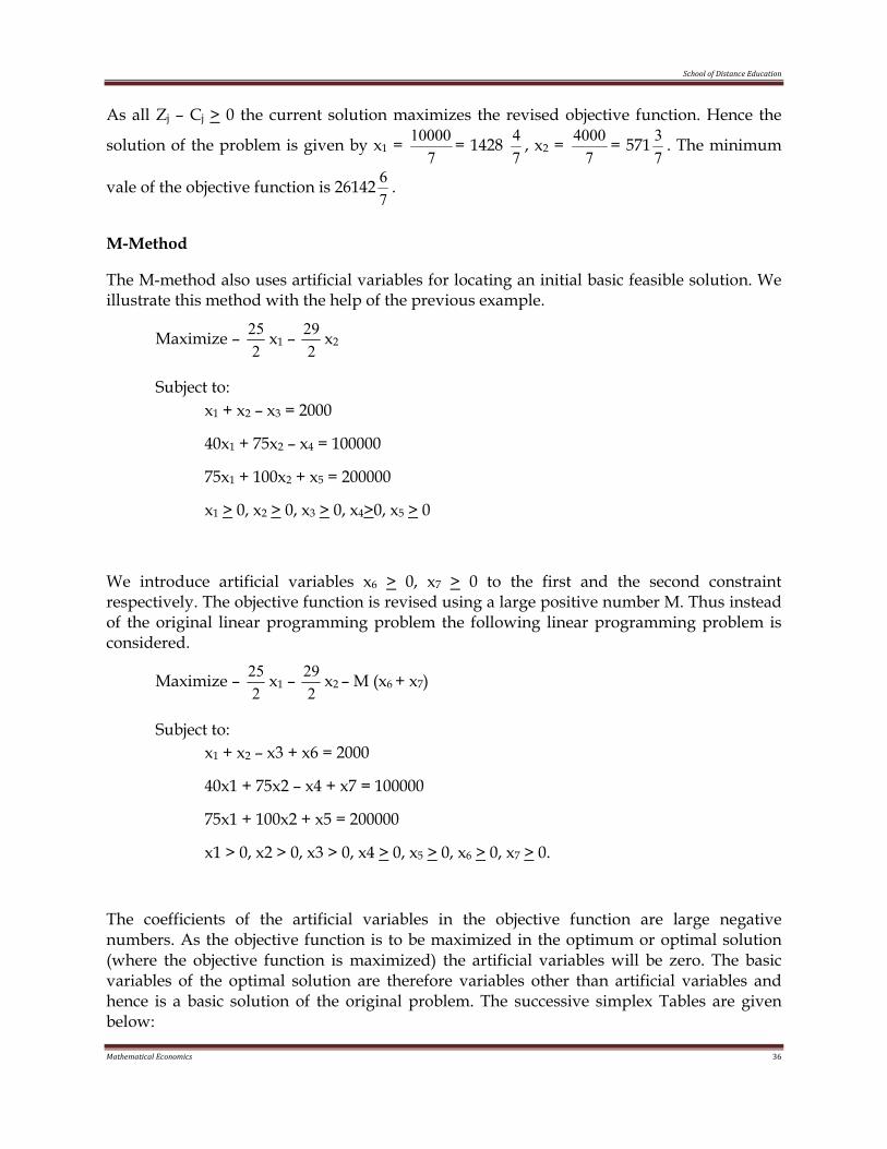
M-Method
The M-method also uses artificial variables for locating an initial basic feasible solution. We illustrate this method with the help of the previous example.
Maximize – 2
25 x1 – 2
29 x2
Subject to: x1 + x2 – x3 = 2000
40x1 + 75x2 – x4 = 100000
75x1 + 100x2 + x5 = 200000
x1 > 0, x2 > 0, x3 > 0, x4>0, x5 > 0
We introduce artificial variables x6 > 0, x7 > 0 to the first and the second constraint respectively. The objective function is revised using a large positive number M. Thus instead of the original linear programming problem the following linear programming problem is considered.
Maximize – 2
25 x1 – 2
29 x2 – M (x6 + x7)
Subject to: x1 + x2 – x3 + x6 = 2000
40x1 + 75x2 – x4 + x7 = 100000
75x1 + 100x2 + x5 = 200000
x1 > 0, x2 > 0, x3 > 0, x4 > 0, x5 > 0, x6 > 0, x7 > 0.
The coefficients of the artificial variables in the objective function are large negative numbers. As the objective function is to be maximized in the optimum or optimal solution (where the objective function is maximized) the artificial variables will be zero. The basic variables of the optimal solution are therefore variables other than artificial variables and hence is a basic solution of the original problem. The successive simplex Tables are given below:
School of Distance Education
Mathematical Economics 37
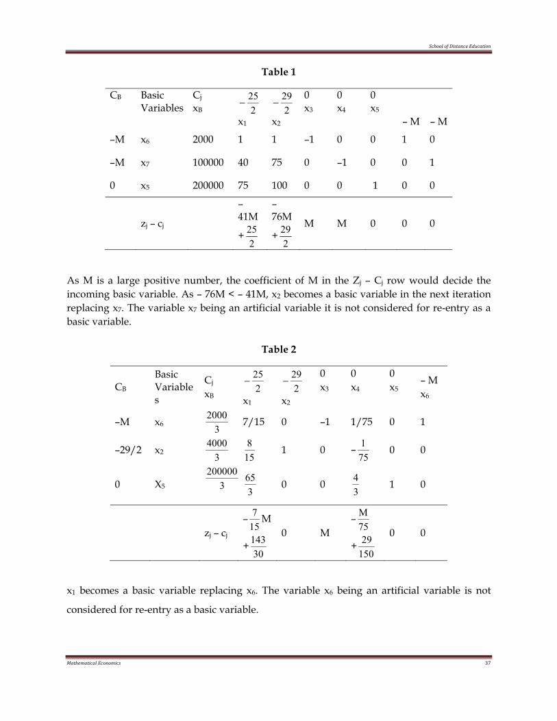
Table 1
CB Basic Variables
Cj
xB 225
−
x1 2
29−
x2
0 x3
0 x4
0 x5
– M – M
–M x6 2000 1 1 –1 0 0 1 0
–M x7 100000 40 75 0 –1 0 0 1
0 x5 200000 75 100 0 0 1 0 0
zj – cj
–41M
+2
25
–76M
+2
29 M M 0 0 0
As M is a large positive number, the coefficient of M in the Zj – Cj row would decide the incoming basic variable. As – 76M < – 41M, x2 becomes a basic variable in the next iteration replacing x7. The variable x7 being an artificial variable it is not considered for re-entry as a basic variable.
Table 2
CB
Basic Variables
Cj
xB 225
−
x1 2
29−
x2
0 x3
0 x4
0 x5
– M x6
–M x6 32000 7/15 0 –1 1/75 0 1
–29/2 x2 34000
158 1 0 –
751 0 0
0 X5 3200000
365 0 0
34 1 0
zj – cj –
157 M
+30
143 0 M
–75M
+15029
0 0
x1 becomes a basic variable replacing x6. The variable x6 being an artificial variable is not
considered for re-entry as a basic variable.
School of Distance Education
Mathematical Economics 38
Table 3
CB Basic Variables
Cj
xB 225
−
x1 2
29−
x2
0 x3
0 x4
0 x5
225
− x1 710000 1 0 –
715
351 0
229
− x2 74000 0 1
78 –
351 0
0 x5 7250000
0 0
7325
2116 1
zj – cj 0 0 14143
352 0
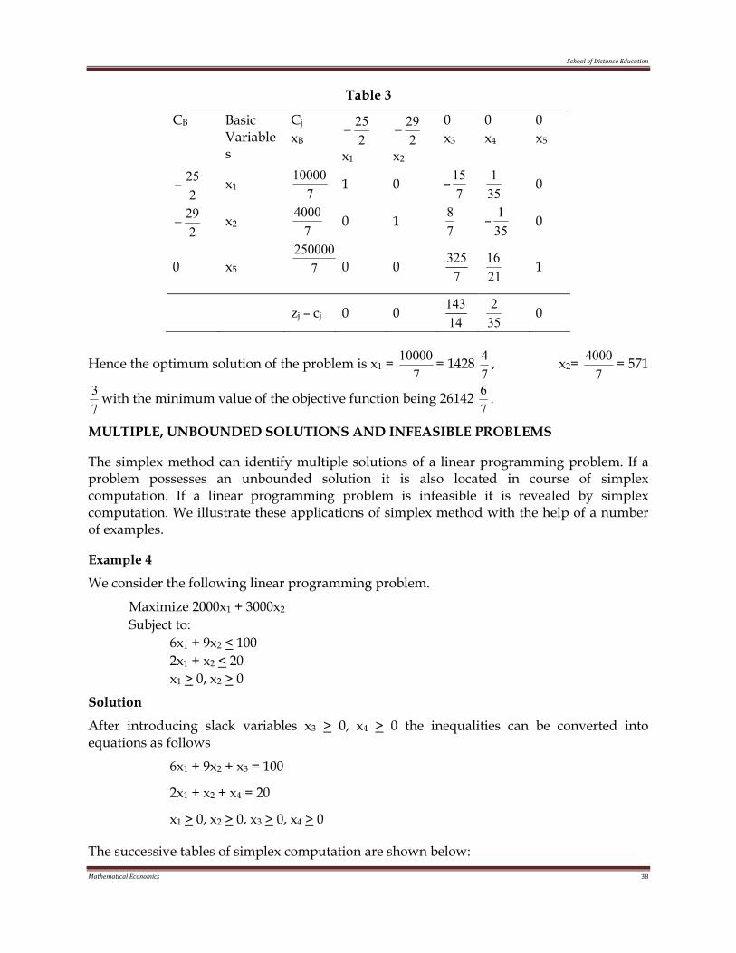
Hence the optimum solution of the problem is x1 = 7
10000 = 1428 74 , x2=
74000 = 571
73 with the minimum value of the objective function being 26142
76 .
MULTIPLE, UNBOUNDED SOLUTIONS AND INFEASIBLE PROBLEMS
The simplex method can identify multiple solutions of a linear programming problem. If a problem possesses an unbounded solution it is also located in course of simplex computation. If a linear programming problem is infeasible it is revealed by simplex computation. We illustrate these applications of simplex method with the help of a number of examples.
Example 4
We consider the following linear programming problem.
Maximize 2000x1 + 3000x2 Subject to: 6x1 + 9x2 < 100 2x1 + x2 < 20 x1 > 0, x2 > 0
Solution
After introducing slack variables x3 > 0, x4 > 0 the inequalities can be converted into equations as follows
6x1 + 9x2 + x3 = 100
2x1 + x2 + x4 = 20
x1 > 0, x2 > 0, x3 > 0, x4 > 0
The successive tables of simplex computation are shown below:
School of Distance Education
Mathematical Economics 39
Table 1
CB Basic Variables
Cj
xB 2000 x1
3000 x2
0 x3
0 x4
0 x3 100 6 9 1 0 0 x4 20 2 1 0 1 zj – cj –2000 –3000 0 0
Table 2
CB Basic Variables
Cj
xB 2000 x1
3000 x2
0 x3
0 x4
0 x2 100/9 2/3 1 1/9 0 0 x4 80/9 4/3 0 –1/9 1
zj – cj 0 0 3000/9 0
Since Zj–Cj > 0 for all the variables, x1=0, x2=100/9 is an optimum solution of the problem. The maximum value of the objective function is 100000/3. However, the Zj–Cj value corresponding to the non basic variable x1 is also zero. This indicates that there is more than one optimum solution of the problem. In order to compute the value of the alternative optimum solution we introduce x1 as a basic variable replacing x4. The subsequent computation is presented in the next Table.
CB Basic Variables
Cj
xB 2000 x1
3000 x2
0 x3
0 x4
3000 x2 320 0 1
61
21
2000 x1 320 1 0 –
121
43
zj – cj 0 0 31000
3000
Thus x1 = 20/3, x2 = 20/3 also maximise the objective function. The maximum value as in the previous solution is 100000/3.
Example 5
Consider the linear programming problem
Maximize 5x1 + 4x2 Subject to: x1 < 7 x1 – x2 < 8 x1 > 0, x2 > 0
School of Distance Education
Mathematical Economics 40
Solution
After introducing slack variables x3 > 0, x4> 0 the corresponding equations are x1 + x3 = 7 x1 – x2 + x4 = 8 x1 > 0, x2 > 0, x3 > 0, x4 > 0.
The successive simplex iterations are shown below:
Table 1
CB Basic Variables
Cj
XB
5 x1
4 x2
0 x3
0 x4
0 x3 7 1 0 1 0 0 x4 8 1 –1 0 1 zj – cj –5 –4 0 0
Table 2
CB Basic Variables
Cj
XB
5 x1
4 x2
0 x3
0 x4
0 x1 7 1 0 1 0 0 x4 1 0 –1 –1 1 zj – cj 0 –4 5 0
z2 – c2 <0 indicates x2 should be introduced as a basic variable in the next iteration. However, both y12< 0, y22 < 0. Thus it is not possible to possible to proceed with the simplex computation any further as you cannot decide which variable will be non basic at the next iteration. This is the criterion for unbounded solution.
If in the course of simplex computation Zj – Cj < 0 but yij < 0 for all i then the problem has no finite solution.
Intuitively, you may observe that the variable x2 in reality unconstrained and can be increased arbitrarily. This is why the solution is unbounded.
Example 6
We consider the linear programming problem given below.
Minimize 200x1 + 300 x2
Subject to: 2x1 + 3x2 > 1200 x1 + x2 < 400 2x1 + 3/2x2 > 900 x1 > 0, x2 > 0.
School of Distance Education
Mathematical Economics 41
Solution
After converting the minimization problem into a maximization problem and introducing slack, surplus, artificial variables the problem can be presented as
Maximize – 200x1 – 300x2
Subject to: 2x1 + 3x2 – x3 + x6 = 1200 x1 + x2 + x4 = 400 2x1 + 3/2x2 – x5 + x7 = 900 x1 > 0, x2> 0, x3 > 0, x4 >, x5 > 0, x6 > 0, x7 > 0.
The variables x6 and x7 are artificial variables. We use two phase method to solve this problem. In Phase I, we use the objective function:
Maximum – x6 – x7
along with the constraints given above. The successive simplex computations are given below:
Table 1
CB Basic Variables
Cj
XB
0 x1
0 x2
0 x3
0 x4
0 x5
–1 x6
–1 x7
–1 x6 1200 2 3 –1 0 0 1 0 0 x4 400 1 1 0 1 0 0 0 –1 x7 900 2 3/2 0 0 –1 0 1 zj – cj –4 –9/2 1 0 1 0 0
Table 2
CB Basic Variables
Cj
XB
0 x1
0 x2
0 x3
0 x4
0 x5
–1 x7
0 x2 400 2/3 1 –1/3 0 0 0 0 x4 0 1/3 0 1/3 1 0 0 –1 x7 300 1 0 1/2 0 –1 1 zj – cj –1 0 –1/2 0 1 0
Table 3
CB Basic Variables
Cj
XB
0 x1
0 x2
0 x3
0 x4
0 x5
–1 x6
0 x2 400 0 1 –1 –2 0 0 0 x1 0 1 0 1 3 0 0 –1 x7 300 0 0 –1/2 –3 –1 1 zj – cj 0 0 1/2 –3 –1 0
School of Distance Education
Mathematical Economics 42
Thus Zj – Cj > 0 for all the variables but the artificial variable x7 is still a basic variable. This indicates that the problem has no feasible solution.
If in course of simplex computation by two phase method one or more artificial variables remain basic variables at the end of Phase I computation, the problem has no feasible solution.
School of Distance Education
Mathematical Economics 43
UNIT 4
DUALITY IN LINEAR PROGRAMMING
In a decision making problem finding the optimum solution alone need not is the objective of the management. They may be interested in the additional informations regarding the impact of technological innovations, economics of resource utilization etc. Such informations can be obtained by considering a related problem called dual problem.
To every LP problem there corresponds another problem called its dual. The original problem is called the primal. Either problem can be considered as primal and the other problem dual. There exists an important theoretical relationship between the primal and its dual which is of practical use also.
Consider the linear programming problem Maximize Z = c1x1 + c2x2 + … + cnxn Subject to a11x1 + a12x2 + … + a1nxn< b1
a21x1 + a22x2 + … + a2nxn < b2 M
am1x1 + am2x2 + … + amn xn < bm x1 > 0, x2 > 0, …, xn > 0
This problem is called primal (in the standard form)
The corresponding dual problem is
Maximize b1y1 + b2y2 + … +bmym Subject to a11y1+a21y2+…+am1ym > c1 a12y1 + a22y2 + … +am2ym > c2
M a1ny1 + a2ny2 + … + amnym > cn y1>0, y2 > 0, …, ym > 0
Example 1
Find the dual of the LP problem
Maximize Z = x1 – x2 + 3x3 Subject to x1 + x2 + x3 < 10 2x1 – x3 < 2 2x1 – 2x2 – 3x3 < 6 x1, x2, x3 > 0
Solution
Dual Minimize w = 10y1 + 2y2 + 6y3 Subject to y1 + 2y2 + 2y3 > 1 y1 – 2y3 > –1 y1 – y2 – 3y3 > 3 y1, y2, y3 > 0
School of Distance Education
Mathematical Economics 44
Example 9
Final the dual. Minimize Z = 3x1 – 2x2 + 4x3 Subject to 3x1 + 5x2 + 4x3 > 7 6x1 + x2 + 3x3 > 4 7x1 – 2x2 – x3 < 10
x1 – 2x2 + 5x3 > 3 4x1 + 7x2 – 2x3 > 2 x1, x2, x3 > 0
Solution
First we convert the primal problem in to standard form.
Maximize Z = –3x1 + 2x2 – 4x3 Subject to – 3x1 – 5x2 – 4x3 < –7 – 6x1 – x2 – 3x3 < – 4 7x1 – 2x2 – x3 < 10 –x1 + 2x2 – 5x3 < –3 –4x1 – 7x2 + 2x3 < –2 xi > 0, i = 1, 2, 3
The we can write the dual directly.
Minimize W = –7y1–4y2 + 10y3 – 3y4 – 2y5
Subject to –3y1 – 6y2 + 7y3 – y4 – 4y5 > –3 –5y1 – y2 – 2y3 + 2y4 – 7y5 > 2 – 4y1 – 3y2 – y3 – 5y4 +2y5> – 4 yi > 0, i = 1, 2, 3, 4, 5
Example 3
Find the Dual
Maximize Z = 5x1 + 12x2 + 4x3 Subject to x1 + 2x2 + x3 < 10 2x1 – x2 + 3x3 = 8 x1, x2, x3 > 0
Solution
The constraints 2x1 – x2 + 3x3 = 8 may be written as two constraints
2x1 – x2 + 3x3 < 8 and 2x1 – x2 + 3x3 > 8 or 2x1 – x2 + 3x3 < 8 and –2x1 + x2 – 3x3 < – 8
so that the Primal is
Maximise Z = 5x1 + 12x2 + 4x3 Subject to x1 + 2x2 + x3 < 10
School of Distance Education
Mathematical Economics 45
2x1 –x2 + 3x3 < 8 –2x1 + x2 –3x3 < –8 x1, x2, x3 > 0
Its dual is
Minimize W = 10y1 + 8y2–8y3 Subject to y1 + 2y2–2y3 > 5 2y1 – y2 + y3 > 12 y1 + 3y2 – 3y3 > 4 y1, y2, y3 > 0 We can summarize the above facts as follows. Primal Dual
n n Variables n Constraints
m m Constraints m Variables
c1, c2, …, cn Cost coefficients Constraint Constants b1, b2,…, bm Constraint constants Cost–coefficients
Variables x1, x2, …, xn > 0 y1, y2, …, ym > 0 Constraints
∑=
≤n
1jijij bxa ∑
=≥
n
1ijjij cya
Objective function Maximize ∑
=
n
1jjjxc Minimize ∑
=
m
1iiiyb
ie., In a primal linear programming problem, the objective is to maximize the objective function with n decision variables and m constraints. The associated dual LPP contains m decision variables with n constraints. Also note that the number of primal variables determines the number of dual constraints, and the number of primal constraints determines the number of dual variables. The per unit contribution of the primal variables (c1, c2, …, cn) becomes the right hand side values of the dual constraints, and the primal RHS values become the per unit contribution of the dual problem.
Example 4
Show using an example that the dual of the dual is primal
Solution
Consider Maximise Z = x1 – x2 + 3x3 Subject to x1 + x2 + x3 < 10 2x1 – x3 < 2 2x1 – 2x2 – 3x3 < 6, x1, x2, x3 > 0
Its dual is
School of Distance Education
Mathematical Economics 46
Minimize 10y1 + 2y2 + 6y3 Subject to y1 + 2y2 + 2y3 > 1 y1 – 2y3 > –1 y1– y2 – 3y3 > 3 y1, y2, y3 > 0
This is an LPP and we can treat this problem as primal writing this in the standard form we get.
Maximize – 10y1 – 2y2 – 6y3 Subject to – y1 – 2y2 – 2y3 < –1 – y1 + 2y3 < 1
– y1 + y2 + 3y3 < – 3 y1, y2, y3 > 0
Its dual is
Minimize – x1 + x2 – 3x3 Subject to – x1 – x2 – x3 > – 10 –2x1 + x3 > –2 – 2x1 + 2x2 + 3x3 > – 6 x1, x2, x3 > 0 i.e., Maximize x1 – x2 + 3x3 Subject to x1 + x2 + x3 < 10 x1 – x3 < 2 2x1 – 2x2 – 3x3 < 6 x1, x2, x3 > 0
which is nothing but the primal
This is not by chance. This is true for any LPP. That is Dual of the dual is primal.
Solution of the Dual
Consider the primal problem
Maximise Z = 45x1 + 8x2 Subject to 5x1 + 20x2 < 400 10x1 + 15x2 < 450
x1, x2 > 0
Its dual is minimize 400y1 + 450y2 Subject to 5y1 + 10y2 > 45 20y1 + 15y2 > 80 y1, y2 > 0
let us solve the problem graphically.
Primal
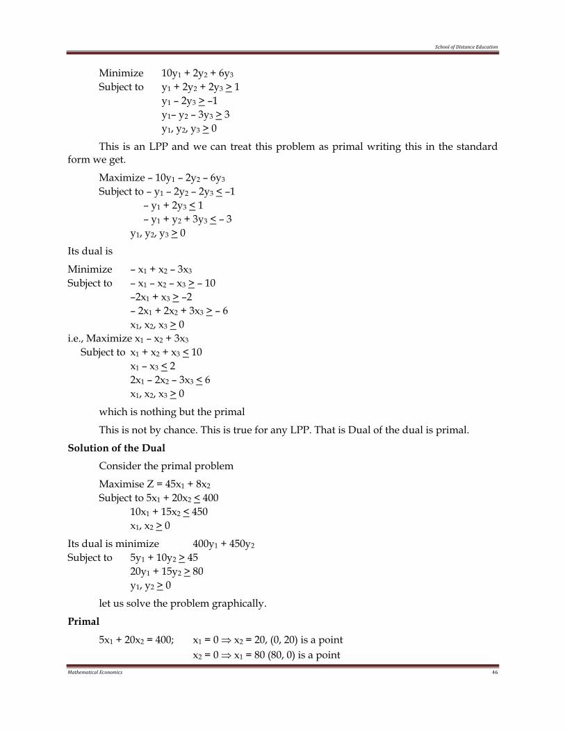
5x1 + 20x2 = 400; x1 = 0 ⇒ x2 = 20, (0, 20) is a point x2 = 0 ⇒ x1 = 80 (80, 0) is a point
School of Distance Education
Mathematical Economics 47
10x1 + 15x2 = 450, x1 = 0 ⇒ x2 = 30 ⇒ (0, 30) is a point x2 = 0 ⇒ x1 = 45 ⇒ (45, 0) is a point
OABC is the feasible region.
Vertex Z = 45x1 + 80x2 O(0, 0) Z = 0
A (0, 20) Z = 1600 B (24, 14) Z = 2200 C(45,0) Z = 2025
Maximum Z*= 2200 *1x = 24, *
2x = 14
Dual
5y1 + 10y2 = 45, y1 = 0 ⇒y2 = 4.5; y2 = 0 ⇒y1 = 9
20y1 + 15y2 = 80, y1 = 0 ⇒y2 = 1580 ; y2 = 0⇒ y1= 4
Vertex 400y1 + 450y2 A(0, 80/15) 400 × 0 + 450 × 80/15 = 2400
B (1, 4) 400 + 1800 = 2200 C (9, 0) 400 × 9 = 3600
0 10 20 30 40 50 60 70 80
10
20
30 A
C
B
0 2 4 6 8 10
A
C
B2
4
6
8
10
Feasible region
School of Distance Education
Mathematical Economics 48
The minimum value is 2200; and the optimum solution is *1y = 1, *
2y =4
We note that the maximum value of the primal objective function is equal to the minimum value of the dual objective function. This is also not by mere chance. We have the following example.
Duality Theorem: If either the primal or the dual problem has a finite optimum solution, then the other problem has a finite optimum solution and the extremes of the linear functions are equal.
If either problem has an unbounded solution, then the other problem has no feasible solution.
Remark: The values of the primal and dual objective functions satisfy the following relationships.
1. If X = (x1,..., xn) is any feasible solution of the primal and Y = (y1, y2, ..., ym) is any feasible solution of the dual then the value of the primal objective function at x will be less than or equal to the value of the dual objective function y.
ie., ∑=
n
1iiixc ∑
=
m
1iii yb
2. At the optimum solution value of the primal objective function = value of the dual objective function.
Economic Interpretation of the Dual Problem
The linear programming problem can be viewed as a resource allocation model in which the objective is to maximize the income or profit subject to available limited resources. Looking at the problem from this stand point, the associated dual problem offers interesting economic interpretations of the LP resource allocation model.
Consider the following resource allocation model. A furniture firm manufactures two items, say tables and chairs, Assume that (for simplicity) wood and labour are the only two resources which are used for the manufacturing of items. It is known that to make a chair it requires 1 unit of wood and 5 man– hours and it yields a profit of 10 Rs. Each table uses 2 units of wood and 6 man hours and yields a profit of Rs. 15. Also it is known that only 28 units of wood and 100 man hours of labour are available. Then the problem is to determine how many tables and chairs should be made so that the profit is a maximum.
The problem is modeled as
Maximize Z = 10x1 + 15x2
Subject to x1 +2x2 < 28 5x1 + 6x2 < 100 x1 > 0, x2 > 0
Let y1 and y2 be the cost per unit of wood and man–hour. Since a chair uses 1 unit of wood and 5 man hours the total worth of resources used for a chair is y1 + 5y2. Similarly the
School of Distance Education
Mathematical Economics 49
total worth of resources used for a table is 2y1 + 6y2. The manufacturer is eager to know whether worth of a chair is greater than or equal to 10, the profit he gets from a chair. Similarly he wishes to know whether the worth of a table is greater than or equal to 15, the profit he gets from a table.
y1 + 5y2 > 10 ie., 2y1 + 6y2 > 15
which are nothing but the dual constraints. He also wishes to minimize the total worth of the resources, ie., min W = 28y1+100y2, which is the dual objective function. At the point of economic equilibrium, maximum of the primal objective function equals minimum of the dual objective function.
Clearly if the worth of a chair is greater than the profit earned from a chair it is not advisable to continue with its production. Similarly if the worth of a table is greater than the profit earned from a table it is better to stop the production of tables. The worth of the resources is also called shadow prices (some times dual prices).
When we solve the above primal and the dual using graphical techniques we get the solution of primal as x1 = 8, x2 = 10 and the maximum profit is 10x1 + 15x2 = 230 and the
solution of the dual as y1= 45y,
415
2 = and minimum of 28y1 + 100y2 = 230. That means y1=4
15
and y2 = 45 are the shadow prices of wood and man hour. That means at the optimum level
the worth of timber is 4
15 Rs./unit and the worth of man hour is 45 /hour. This in turn
implies that if the manufacturer can get timber at less than Rs. 415 per unit and man hour at
less than Rs. 45 per hour he can get extra profits. In this particular example the
manufacturer uses all the resources (x1+ 2x2 = 8 + 20 = 28 and 5x1 + 6x2 = 40 + 160 = 200). In some cases it can happen that some resources are not fully utilized and there is idle capacity. The idle capacity has no contribution to the profit. In such a case, at the optimal value, manufacturer cannot get any more profit by adding an extra unit of this resource.
It is to note that the shadow price of a resource indicates the amount by which the objective function would increase if we increase the supply of the resource by one unit. That simply means that if the supply of the timber is increased by 1 unit the objective function would increase from 230 to 935/4. This is so since in that case the problem is
Maximize Z = 10x1 + 15x2
Subject to x1 + 2x2 < 29 5x1 + 6x2 < 100 x1 > 0, x2 > 0.
Solving it is we get (solve!) x1 = 26/4 and x2 45/4 and Z*= 10 × 26/4 + 15 × 45/4 = 935/4 and the increase is (935/4)– 230 = 15/4, the value of y1. Similarly when we increase the value of man–hour from 100 to 101 we get x1 = 34/4, x2=39/4, Z = 935/4 (Do it graphically) and the increase is (935/4)–230 = 15/4, the value of the dual variable y2.
School of Distance Education
Mathematical Economics 50
EXERCISES
II. Fill up the blanks
1. …….variables are introduced to make…… type inequalities equations.
2. A system with m equations and n variables has at most ……… basic solutions.
3. A basic solution with m equations and n variables has ……… variables equal to zero.
4. A basic feasible solution is a basic solution whose variables are………
5. The maximum number of basic feasible solutions in a system with m equations and n variables is ……………
6. In a linear programming problem every …………… point of the Convex set of feasible solutions is a ……………… solution of the problem.
7. The objective function of a linear programming problem is maximized or minimized at a ………………. solution.
III. Very Short Answer Questions
8. What is an objective function?
9. What are constraints?
10. Define feasible solution.
11. Define basic feasible solution.
12. Define feasible region.
13. Define alternate optimum solution.
14. What do you mean by unbounded solution.
15. What is infeasible solution?
16. Define a slack variable.
17. Define a surplus variable.
18. Define artificial variable.
19. What is a dual problem?
20. What is primal?
21. What is a shadow price?
22. What are dual variables?
School of Distance Education
Mathematical Economics 51
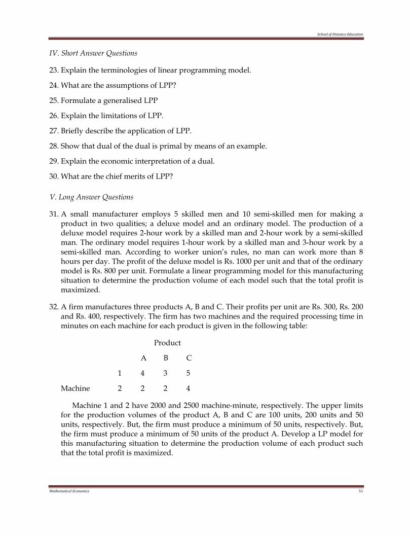
IV. Short Answer Questions
23. Explain the terminologies of linear programming model.
24. What are the assumptions of LPP?
25. Formulate a generalised LPP
26. Explain the limitations of LPP.
27. Briefly describe the application of LPP.
28. Show that dual of the dual is primal by means of an example.
29. Explain the economic interpretation of a dual.
30. What are the chief merits of LPP?
V. Long Answer Questions
31. A small manufacturer employs 5 skilled men and 10 semi-skilled men for making a product in two qualities; a deluxe model and an ordinary model. The production of a deluxe model requires 2-hour work by a skilled man and 2-hour work by a semi-skilled man. The ordinary model requires 1-hour work by a skilled man and 3-hour work by a semi-skilled man. According to worker union’s rules, no man can work more than 8 hours per day. The profit of the deluxe model is Rs. 1000 per unit and that of the ordinary model is Rs. 800 per unit. Formulate a linear programming model for this manufacturing situation to determine the production volume of each model such that the total profit is maximized.
32. A firm manufactures three products A, B and C. Their profits per unit are Rs. 300, Rs. 200 and Rs. 400, respectively. The firm has two machines and the required processing time in minutes on each machine for each product is given in the following table:
Product
A B C
1 4 3 5
Machine 2 2 2 4
Machine 1 and 2 have 2000 and 2500 machine-minute, respectively. The upper limits for the production volumes of the product A, B and C are 100 units, 200 units and 50 units, respectively. But, the firm must produce a minimum of 50 units, respectively. But, the firm must produce a minimum of 50 units of the product A. Develop a LP model for this manufacturing situation to determine the production volume of each product such that the total profit is maximized.
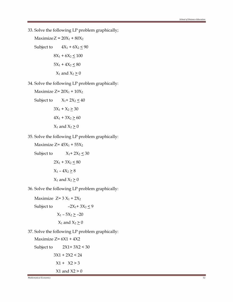
School of Distance Education
Mathematical Economics 52
33. Solve the following LP problem graphically;
Maximize Z = 20X1 + 80X2
Subject to 4X1 + 6X2 < 90
8X1 + 6X2 < 100
5X1 + 4X2 < 80
X1 and X2 > 0
34. Solve the following LP problem graphically:
Maximize Z= 20X1 + 10X2
Subject to X1+ 2X2 < 40
3X1 + X2 > 30
4X1 + 3X2 > 60
X1 and X2 > 0
35. Solve the following LP problem graphically:
Maximize Z= 45X1 + 55X2
Subject to X1+ 2X2 < 30
2X1 + 3X2 < 80
X1 – 4X2 > 8
X1 and X2 > 0
36. Solve the following LP problem graphically:
Maximize Z= 3 X1 + 2X2
Subject to –2X1+ 3X2 < 9
X1 – 5X2 > –20
X1 and X2 > 0
37. Solve the following LP problem graphically:
Maximize Z= 6X1 + 4X2
Subject to 2X1+ 3X2 < 30
3X1 + 2X2 < 24
X1 + X2 > 3
X1 and X2 > 0
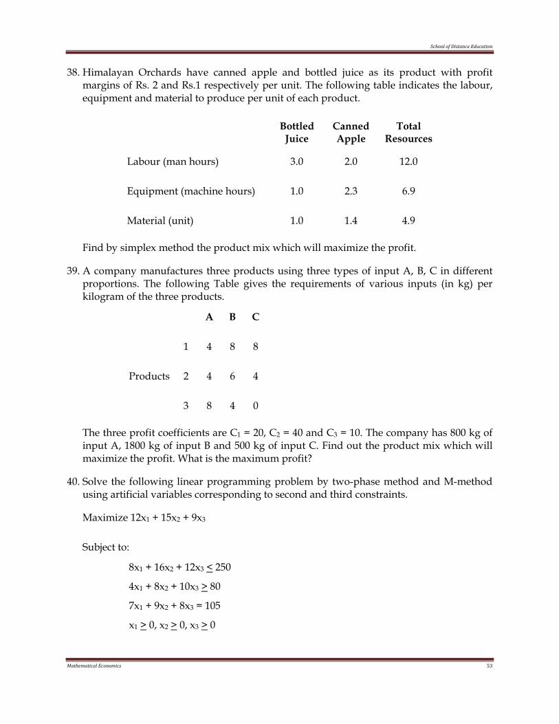
School of Distance Education
Mathematical Economics 53
38. Himalayan Orchards have canned apple and bottled juice as its product with profit margins of Rs. 2 and Rs.1 respectively per unit. The following table indicates the labour, equipment and material to produce per unit of each product.
Bottled Juice
Canned Apple
Total Resources
Labour (man hours) 3.0 2.0 12.0
Equipment (machine hours) 1.0 2.3 6.9
Material (unit) 1.0 1.4 4.9
Find by simplex method the product mix which will maximize the profit.
39. A company manufactures three products using three types of input A, B, C in different proportions. The following Table gives the requirements of various inputs (in kg) per kilogram of the three products.
A B C
Products
1 4 8 8
2 4 6 4
3 8 4 0
The three profit coefficients are C1 = 20, C2 = 40 and C3 = 10. The company has 800 kg of input A, 1800 kg of input B and 500 kg of input C. Find out the product mix which will maximize the profit. What is the maximum profit?
40. Solve the following linear programming problem by two-phase method and M-method using artificial variables corresponding to second and third constraints.
Maximize 12x1 + 15x2 + 9x3
Subject to:
8x1 + 16x2 + 12x3 < 250
4x1 + 8x2 + 10x3 > 80
7x1 + 9x2 + 8x3 = 105
x1 > 0, x2 > 0, x3 > 0
School of Distance Education
Mathematical Economics 54
41. Solve the linear programming problem by simplex method and give your comments. Maximise x1 + x2
Subject to:
– 2x1 + x2 < 1
x1 < 2
x1 + x2 < 3
x1 > 0, x2 > 0
42. Solve the following linear programming problem by simplex method and give your comments.
Maximise 3x1 + 2x2
Subject to;
x1 – x2 < 1
x1 + x2 > 3
x1 > 0, x2 > 0
43. Write the dual of the LPP
Max Z = – 3x1 – x2
Subject to x1 + x2 > 1
x1 + 3x2 > 2
x1, x2 > 0
44. Write the dual of the LPP
Max Z = 3x1 + 4x2
Subject to x1 – x2 < 1
x1 + x2 < 4
x1 – 3x2 < 3
x1, x2> 0
45. Write the dual of the LPP
Max Z = 3x1 + 2x2
Subject to x1 – x2 < 1
x1 + x2 > 3
x1, x2 > 0
School of Distance Education
Mathematical Economics 55
46. Describe feasible solution and basic feasible solution of a linear programming problem
(LPP). Write down the dual of the following LPP:
Maximize Z = 5x1 + 10x2 + 15x3 subject to the constraints x1 + 2x2 + x3 < 1
x1 + 3x3 < 5
x1 + x2 < 2
x1, x2, x3 > 0.
School of Distance Education
Mathematical Economics 56
Module III
THEORY OF GAMES
UNIT 1: GAME THEORY
In problems considered in LPP the assumption has been that there is single decision maker whose interest lies in choosing the variables in such a way as to optimize the objective function. This type of problems can be considered as a game between a rational decision maker and nature. Since nature is generally not considered to be rational, the decision maker may choose to use something better than the most conservative strategy to try to maximize his gain. However, if the decision maker’s opponent is also rational and is trying to maximize his gain, the problem becomes a decision problem involving conflict of interests. In this case, very conservative strategies must be used by both the parties. Mathematical models of such situations and their solutions is the essence of game theory.
Definition: Game is defined as an activity between two or more persons involving moves by each person according to a set of rules, at the end of which each person receive some benefit or satisfaction or suffers loss.
A set of rules defines the game. Going through the se of rules once by the participation defines a play.
The games are classified based on the following characteristics.
1. Chance or strategy: If in a game the moves are determined by chance, we call it a game of chance, if they are determined by skill, it is a game of strategy. In general a game may involve partly strategy and partly chance.
2. Number of Persons: A game is called an n-person game if the number of persons playing it is n.
3. Number of moves: The number of moves may be finite or infinite.
4. Number of alternative available to each person per move: These also may be finite of infinite.
A finite game has a finite number of moves, each involving a finite number alternative. Other wise the game is infinite.
5. Information available to players of the past moves of the other players: The two extreme cases are, (a) no information at all (b) complete information available. There can be cases in between in which information is partly available.
6. Pay off: It is a quantitative measure of satisfaction a person gets at the end of the play. It is real a valued function of the variables in the game.
School of Distance Education
Mathematical Economics 57
Let Pi be the pay off to the person, Pi, i = 1, 2, …, n, in an n-person game.
Then if ∑=
n
1iiP = 0, the game is said to be a zero-sum game.
TYPES OF GAMES
Games can be of several types. Important ones are as follows:
(1) Two-person games and n-person games. In two-person games the players may have many possible choices open to them for each play of the game but the number of players remains only two. But games can as well involve many people as active participants, each with his own set of choices for each play of the game. In case of three players, it can be named as three-person game. Thus, in case of more than two persons, the game is generally named as n person game.
(2) Zero sum and non-zero sum game. A zero sum game is one in which the sum of the payments to all the competitors is zero for every possible outcome of the game. In other words, in such a game the sum of the points won equals the sum of the points lost i.e., one player wins at the expense of the other (others). Two-person matrix game is always zero sum game since one player loses what the other wins. But in a non-zero sum game the sum of the payoffs from any play of the game may be either positive or negative but not zero.
Although some games involve more than two players, we will restrict our attention to two-person games. Suppose we consider the decision problem in which two rational players, Player I and Player II, each have a set of possible actions available to them. Each player might be a foot ball team, a company, an army, a contractor or a politician. Suppose players I and II have m actions a1, a2, …, am and n actions b1, b2, …, bn available, respectively. On each play of the game, each player selects a single action from his set of actions. The consequence of this decision by both players is a specific return or pay off. If the pay off is non-zero, it represents a gain or loss, to player I. We will consider the case where Player I’s gain is Player II’s loss and conversely. No units enter or leave the game. This type of game is called a two-person zero sum game. Thus, with out loss of generality, we can always consider the pay off as being from Player II to Player I. Since Player I’s gain is Player II’s loss, and vice versa, the gain to Player II is the negative of the gain to Player I.
In general, we will let aij represent the pay off from Player II to Player I if Player I chooses action ai and Player II chooses action bj. The set of all possible pay offs is displayed in a table called the pay off matrix, which represents the pay off from Player II to Player I for all possible actions by both players. The following table could be considered Player I’s gain table or Player II’s loss table.
If Player I chooses action ai, we will say that he plays row i. Likewise, if Player II chooses action bj, we will say that he plays column j.
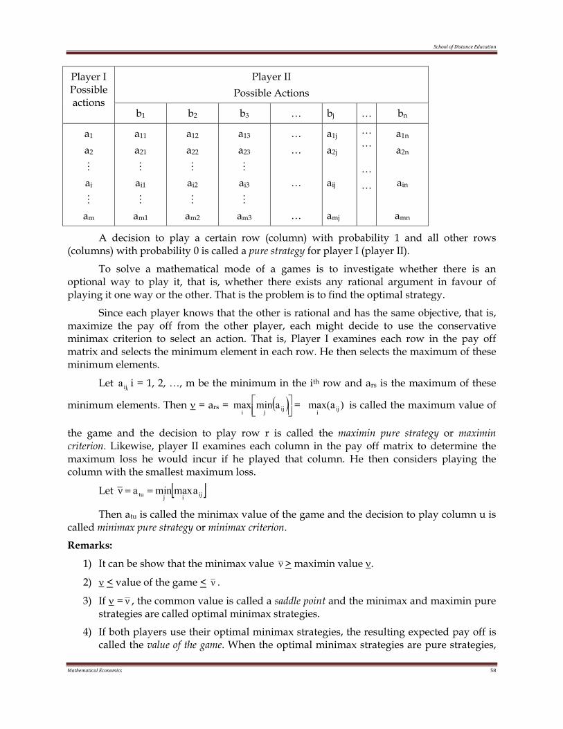
School of Distance Education
Mathematical Economics 58
Player I Possible actions
Player II Possible Actions
b1 b2 b3 … bj … bn
a1
a2 M ai M
am
a11
a21
M ai1
M am1
a12
a22
M ai2
M am2
a13
a23
M ai3
M am3
… …
…
…
a1j
a2j
aij
amj
… … … …
a1n
a2n
ain
amn
A decision to play a certain row (column) with probability 1 and all other rows (columns) with probability 0 is called a pure strategy for player I (player II).
To solve a mathematical mode of a games is to investigate whether there is an optional way to play it, that is, whether there exists any rational argument in favour of playing it one way or the other. That is the problem is to find the optimal strategy.
Since each player knows that the other is rational and has the same objective, that is, maximize the pay off from the other player, each might decide to use the conservative minimax criterion to select an action. That is, Player I examines each row in the pay off matrix and selects the minimum element in each row. He then selects the maximum of these minimum elements.
Let iija i = 1, 2, …, m be the minimum in the ith row and ars is the maximum of these
minimum elements. Then ν = ars = ( )⎥⎦⎤
⎢⎣⎡
ijjiaminmax = )a(max iji
is called the maximum value of
the game and the decision to play row r is called the maximin pure strategy or maximin criterion. Likewise, player II examines each column in the pay off matrix to determine the maximum loss he would incur if he played that column. He then considers playing the column with the smallest maximum loss.
Let [ ]ijijtu amaxminaν ==
Then atu is called the minimax value of the game and the decision to play column u is called minimax pure strategy or minimax criterion.
Remarks:
1) It can be show that the minimax value ν > maximin value ν.
2) ν < value of the game < ν .
3) If ν = ν , the common value is called a saddle point and the minimax and maximin pure strategies are called optimal minimax strategies.
4) If both players use their optimal minimax strategies, the resulting expected pay off is called the value of the game. When the optimal minimax strategies are pure strategies,
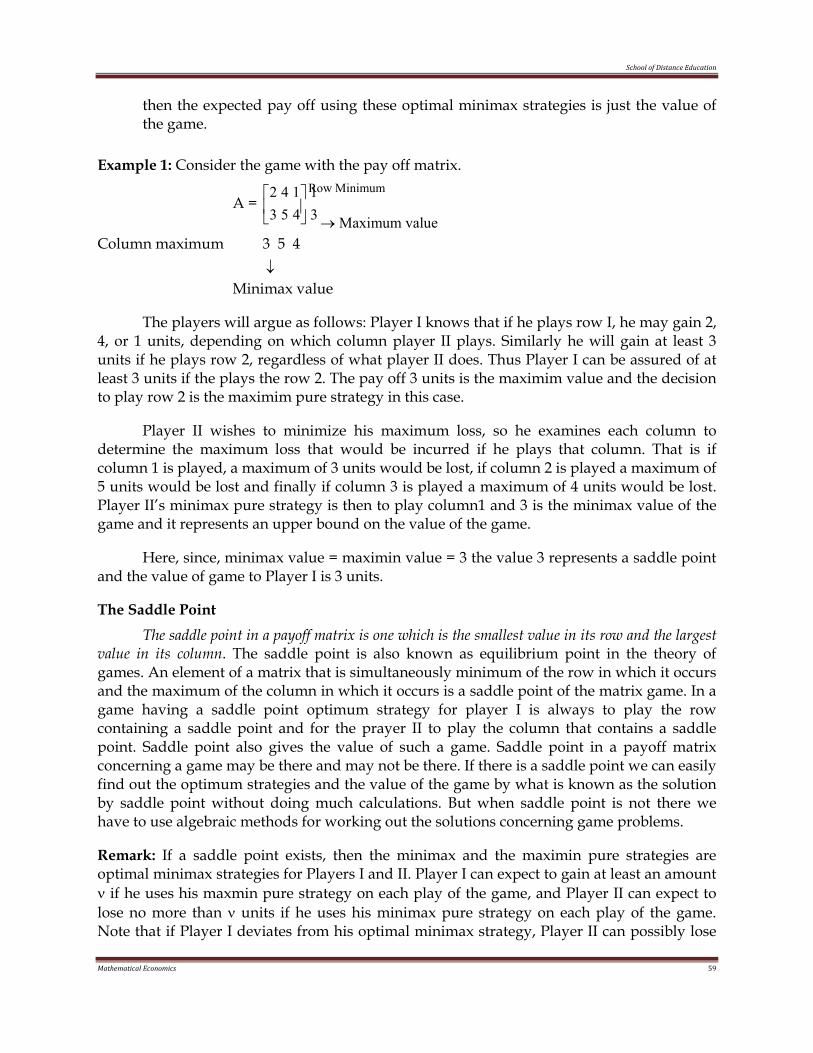
School of Distance Education
Mathematical Economics 59
then the expected pay off using these optimal minimax strategies is just the value of the game.
Example 1: Consider the game with the pay off matrix.
A = 31
41
54
32
⎥⎦
⎤⎢⎣
⎡
Column maximum 3 5 4
Minimax value
The players will argue as follows: Player I knows that if he plays row I, he may gain 2, 4, or 1 units, depending on which column player II plays. Similarly he will gain at least 3 units if he plays row 2, regardless of what player II does. Thus Player I can be assured of at least 3 units if the plays the row 2. The pay off 3 units is the maximim value and the decision to play row 2 is the maximim pure strategy in this case.
Player II wishes to minimize his maximum loss, so he examines each column to determine the maximum loss that would be incurred if he plays that column. That is if column 1 is played, a maximum of 3 units would be lost, if column 2 is played a maximum of 5 units would be lost and finally if column 3 is played a maximum of 4 units would be lost. Player II’s minimax pure strategy is then to play column1 and 3 is the minimax value of the game and it represents an upper bound on the value of the game.
Here, since, minimax value = maximin value = 3 the value 3 represents a saddle point and the value of game to Player I is 3 units.
The Saddle Point The saddle point in a payoff matrix is one which is the smallest value in its row and the largest value in its column. The saddle point is also known as equilibrium point in the theory of games. An element of a matrix that is simultaneously minimum of the row in which it occurs and the maximum of the column in which it occurs is a saddle point of the matrix game. In a game having a saddle point optimum strategy for player I is always to play the row containing a saddle point and for the prayer II to play the column that contains a saddle point. Saddle point also gives the value of such a game. Saddle point in a payoff matrix concerning a game may be there and may not be there. If there is a saddle point we can easily find out the optimum strategies and the value of the game by what is known as the solution by saddle point without doing much calculations. But when saddle point is not there we have to use algebraic methods for working out the solutions concerning game problems.
Remark: If a saddle point exists, then the minimax and the maximin pure strategies are optimal minimax strategies for Players I and II. Player I can expect to gain at least an amount ν if he uses his maxmin pure strategy on each play of the game, and Player II can expect to lose no more than ν units if he uses his minimax pure strategy on each play of the game. Note that if Player I deviates from his optimal minimax strategy, Player II can possibly lose
Row Minimum
→ Maximum value
↓
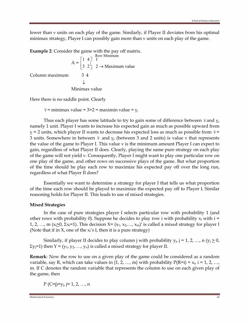
School of Distance Education
Mathematical Economics 60
fewer than ν units on each play of the game. Similarly, if Player II deviates from his optimal minimax strategy, Player I can possibly gain more than ν units on each play of the game.
Example 2: Consider the game with the pay off matrix.
A = 21
24
31
⎥⎦
⎤⎢⎣
⎡
Column maximum 3 4
Minimax value
Here there is no saddle point. Clearly
ν = minimax value = 3>2 = maximin value = ν.
Thus each player has some latitude to try to gain some of difference between ν and ν, namely 1 unit. Player I wants to increase his expected gain as much as possible upward from ν = 2 units, which player II wants to decrease his expected loss as much as possible from ν = 3 units. Somewhere in between ν and ν, (between 3 and 2 units) is value ν that represents the value of the game to Player I. This value ν is the minimum amount Player I can expect to gain, regardless of what Player II does. Clearly, playing the same pure strategy on each play of the game will not yield ν. Consequently, Player I might want to play one particular row on one play of the game, and other rows on successive plays of the game. But what proportion of the time should he play each row to maximize his expected pay off over the long run, regardless of what Player II does?
Essentially we want to determine a strategy for player I that tells us what proportion of the time each row should be played to maximize the expected pay off to Player I. Similar reasoning holds for Player II. This leads to use of mixed strategies.
Mixed Strategies
In the case of pure strategies player I selects particular row with probability 1 (and other rows with probability 0). Suppose he decides to play row i with probability xi with i = 1, 2, …, m (xi>0, Σxi=1). This decision X= (x1, x2,…, xm)′ is called a mixed strategy for player I (Note that if in X, one of the xi’s I, then it is a pure strategy)
Similarly, if player II decides to play column j with probability yj, j = 1, 2, …, n (yj > 0, Σyj=1) then Y = (y1, y2, …, yn) is called a mixed strategy for player II.
Remark: Now the row to use on a given play of the game could be considered as a random variable, say R, which can take values in {1, 2, …, m} with probability P(R=i) = xi, i = 1, 2, …, m. If C denotes the random variable that represents the column to use on each given play of the game, then
P (C=j)=yj, j= 1, 2, …, n
Row Minimum
→ Maximum value
↓
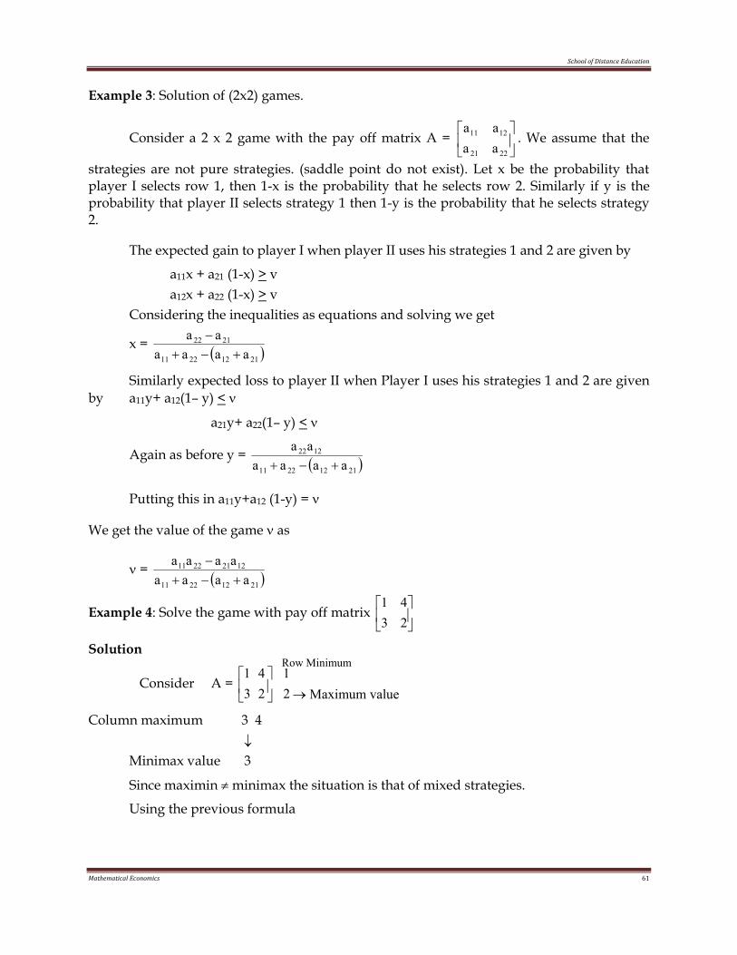
School of Distance Education
Mathematical Economics 61
Example 3: Solution of (2x2) games.
Consider a 2 x 2 game with the pay off matrix A = ⎥⎦
⎤⎢⎣
⎡
2221
1211
aaaa
. We assume that the
strategies are not pure strategies. (saddle point do not exist). Let x be the probability that player I selects row 1, then 1-x is the probability that he selects row 2. Similarly if y is the probability that player II selects strategy 1 then 1-y is the probability that he selects strategy 2.
The expected gain to player I when player II uses his strategies 1 and 2 are given by
a11x + a21 (1-x) > v a12x + a22 (1-x) > v Considering the inequalities as equations and solving we get
x = ( )21122211
2122
aaaaaa
+−+−
Similarly expected loss to player II when Player I uses his strategies 1 and 2 are given by a11y+ a12(1– y) < ν
a21y+ a22(1– y) < ν
Again as before y = ( )21122211
1222
aaaaaa
+−+
Putting this in a11y+a12 (1-y) = ν
We get the value of the game ν as
ν = ( )21122211
12212211
aaaaaaaa+−+
−
Example 4: Solve the game with pay off matrix ⎥⎦
⎤⎢⎣
⎡2341
Solution
Consider A = 21
24
31
⎥⎦
⎤⎢⎣
⎡
Column maximum 3 4
Minimax value 3
Since maximin ≠ minimax the situation is that of mixed strategies.
Using the previous formula
Row Minimum
→ Maximum value
↓
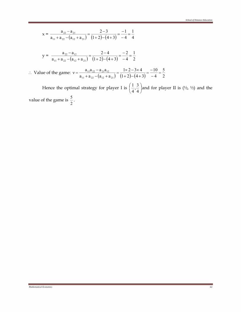
School of Distance Education
Mathematical Economics 62
x = ( ) ( ) ( ) 41
41
342132
aaaaaa
21122211
2122 =−−
=+−+
−=
+−+−
y = ( ) ( ) ( ) 21
42
342142
aaaaaa
21122211
1222 =−−
=+−+
−=
+−+−
∴ Value of the game: ( ) ( ) ( ) 25
410
34214321
aaaaaaaaν
21122211
12212211 =−−
=+−+×−×
=+−+
−=
Hence the optimal strategy for player I is ⎟⎠⎞
⎜⎝⎛
43,
41 and for player II is (½, ½) and the
value of the game is 25 .
School of Distance Education
Mathematical Economics 63
UNIT 2
LINEAR PROGRAMMING SOLUTION OF GAMES
Game theory bears a strong relationship to linear programming, in the sense that a two-person zero-sum game can be expressed as a linear program and vice-versa.
Consider the game with the payoff matrix.
Player A ⎥⎥⎥⎥
⎦
⎤
⎢⎢⎢⎢
⎣
⎡
mn2m1m
n22221
n11211
aaa
aa1aaa
3
21
M
We assume that there is no saddle point. That means the strategies are not pure strategies.
Problem of Player A is to determine the probabilities x1, x2, ..., xm of selecting the strategies 1, 2, ..., m respectively, so as to maximize his minimum expected gain.
Now, the expected gains ν1, v2, ..., vn of Player A against B’s strategies are given by
ν1 = a11x1 + a21x2 + ...+am1xm
ν2 = a12x1 + a22x2 + ...+am2xm M
νn = a1nx1 + a2nx2 + ...+amnxm
The Player A has to select x1, x2, ..., xm ⎟⎠
⎞⎜⎝
⎛=≥ ∑
=
m
1iii 1x,0x that will yield }v{minmax jxi
.
That is ⎭⎬⎫
⎩⎨⎧
⎟⎠
⎞⎜⎝
⎛ ∑ ∑∑= ==
m
1i
m
1iiini2i
m
1ii1ix
xa,...xa,xaminmaxi
Subject to x1 + x2 + ... + xm = 1, x1 > 0, i = 1, 2, ..., m.
Let ν = min ⎟⎠
⎞⎜⎝
⎛ ∑∑∑===
m
1iiin
m
1ii2i
m
1ii1i xa...,xa,xa .
This implies that, ∑=
=≥m
1iiij .n...1,2,j ν,xa
Player A’s problem thus can be written as
Maximize Z = ν,
subject to ∑=
=≥m
1iiij n...1,2,j ν,xa
x1 + x2 + ...+ xm = 1, xi > 0 i=1,2,..., m.
School of Distance Education
Mathematical Economics 64
Assume that ν > 0. (If ν < 0, modify that payoff matrix by adding a suitable constant C > 0 to all entries of (aij) and work with the modified matrix. After the optimum solution is obtained, the true value of the game is obtained by subtracting that constant C).
Let νxx i
i =′ , for i = 1, 2, ..., m.
Then the problem becomes,
Maximize ν = Minimize ∑∑==
′==m
1ii
m
1i
i xνx
ν1 .
ie., Minimize .x...xxZ m21 ′++′+′=′ Subject to a11 ,1xa...xax m1m2211 ≥′′++′+′ ,1xa...xaxa m2m222112 ≥′++′+′
M ,1xa...xaxa mmn2n21n1 ≥′++′+′
.m,...,2,1i,0x1 =≥′
Similarly, Player B’s optimal strategies y1, y2, ..., yn are determined by solving the problem.
⎭⎬⎫
⎩⎨⎧
⎟⎟⎠
⎞⎜⎜⎝
⎛ ∑∑∑===
n
1jjmj
n
1jjj2
n
1jjj1y
ya,...,ya,yamaxminj
Subject to y1+y2+...+yn=1 yi > 0, i = 1, 2, ..., n.
Let max ⎟⎟⎠
⎞⎜⎜⎝
⎛ ∑∑∑===
n
1jjmj
n
1jjj2
n
1jjj1 ya,...,ya,ya = ν.
This implies ∑=
=≤n
1jjj1 m.1,2,...,i ν,ya
Proceeding on the lines as in the case of problem of Player A, problem of Player B is
Minimize n21 y...yyω ′++′+′=′ Subject to ,1ya...yaya nn1212111 ≤′++′+′
.n,...,2,1i,0y1ya...yaya
1ya...yaya
1
nmn2m21m1
nn2222121
=≥′≤′++′+′
≤′++′+′
M
Remark: It can be seen that B’s problem is the dual of A’s problem. (verify!) This means that the optimal solution of one problem automatically yields the optimal solution of the other.
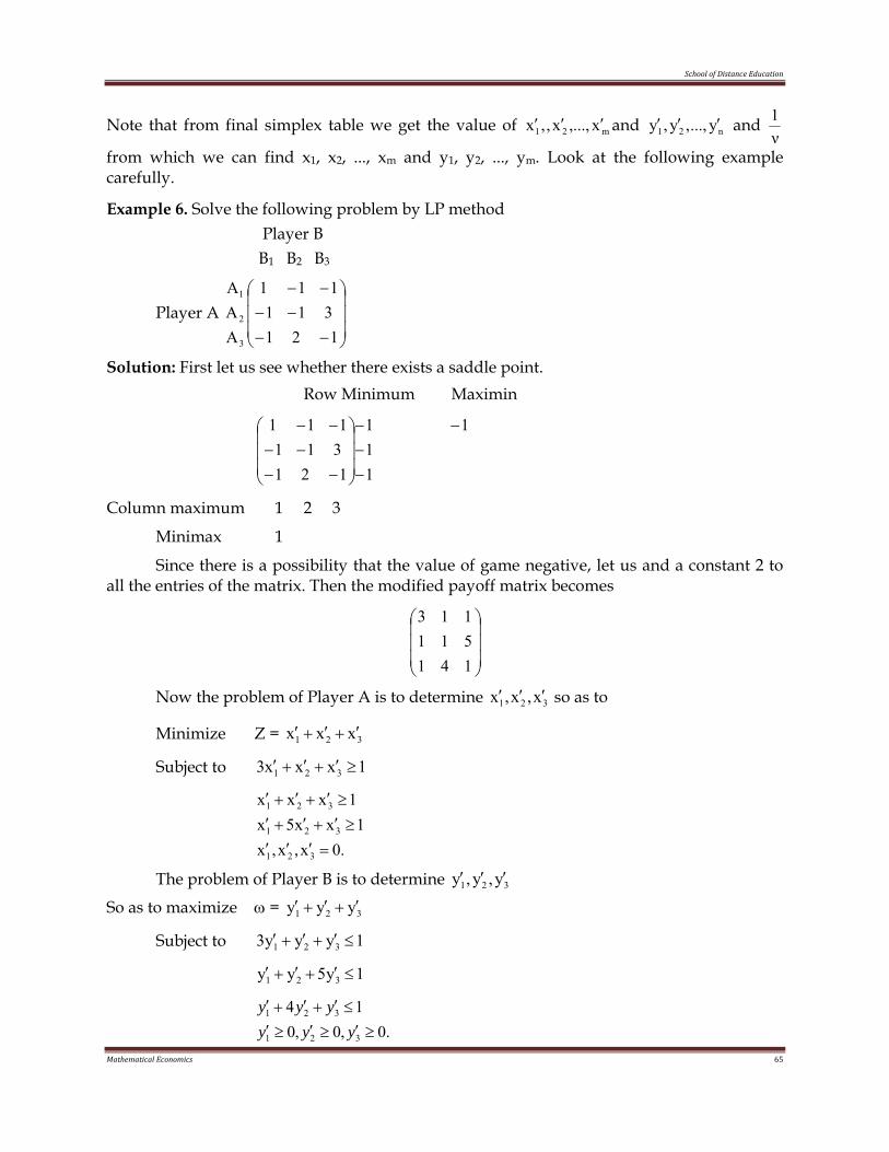
School of Distance Education
Mathematical Economics 65
Note that from final simplex table we get the value of m21 x,...,x,,x ′′′ and n21 y...,,y,y ′′′ and ν1
from which we can find x1, x2, ..., xm and y1, y2, ..., ym. Look at the following example carefully. Example 6. Solve the following problem by LP method
Player B B1 B2 B3
Player A ⎟⎟⎟
⎠
⎞
⎜⎜⎜
⎝
⎛
−−−−
−−
121311111
AAA
3
2
1
Solution: First let us see whether there exists a saddle point. Row Minimum Maximin
1
111
121311111 −
−−−
⎟⎟⎟
⎠
⎞
⎜⎜⎜
⎝
⎛
−−−−
−−
Column maximum 1 2 3
Minimax 1
Since there is a possibility that the value of game negative, let us and a constant 2 to all the entries of the matrix. Then the modified payoff matrix becomes
⎟⎟⎟
⎠
⎞
⎜⎜⎜
⎝
⎛
141511113
Now the problem of Player A is to determine 321 x,x,x ′′′ so as to
Minimize Z = 321 xxx ′+′+′
Subject to 1xxx3 321 ≥′+′+′
.0x,x,x
1xx5x1xxx
321
321
321
=′′′≥′+′+′≥′+′+′
The problem of Player B is to determine 321 y,y,y ′′′
So as to maximize ω = 321 yyy ′+′+′
Subject to 1yyy3 321 ≤′+′+′
1y5yy 321 ≤′+′+′
.0,0,014
321
321
≥′≥′≥′≤′+′+′
yyyyyy
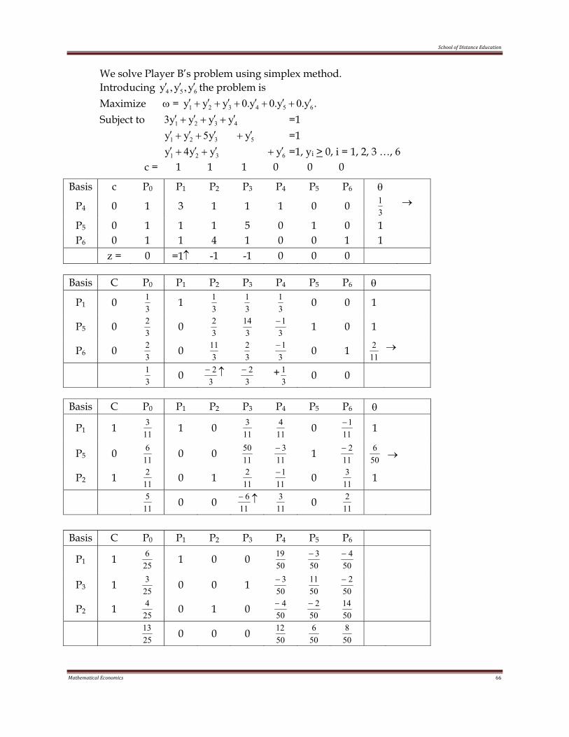
School of Distance Education
Mathematical Economics 66
We solve Player B’s problem using simplex method. Introducing 654 y,y,y ′′′ the problem is Maximize ω = .y.0y.0y.0yyy 654321 ′+′+′+′+′+′ Subject to 4321 yyyy3 ′+′+′+′ =1 5321 yy5yy ′+′+′+′ =1 6321 yyy4y ′+′+′+′ =1, yi > 0, i = 1, 2, 3 …, 6 c = 1 1 1 0 0 0
Basis c P0 P1 P2 P3 P4 P5 P6 θ
P4 0 1 3 1 1 1 0 0 31 →
P5 0 1 1 1 5 0 1 0 1 P6 0 1 1 4 1 0 0 1 1 z = 0 =1↑ -1 -1 0 0 0
Basis C P0 P1 P2 P3 P4 P5 P6 θ
P1 0 31 1
31
31
31 0 0 1
P5 0 32 0
32
314
31− 1 0 1
P6 0 32 0
311
32
31− 0 1
112 →
31 0
32− ↑
32− +
31 0 0
Basis C P0 P1 P2 P3 P4 P5 P6 θ
P1 1 113 1 0
113
114 0
111− 1
P5 0 116 0 0
1150
113− 1
112−
506 →
P2 1 112 0 1
112
111− 0
113 1
115 0 0
116− ↑
113 0
112
Basis C P0 P1 P2 P3 P4 P5 P6
P1 1 256 1 0 0
5019
503−
504−
P3 1 253 0 0 1
503−
5011
502−
P2 1 254 0 1 0
504−
502−
5014
2513 0 0 0
5012
506
508
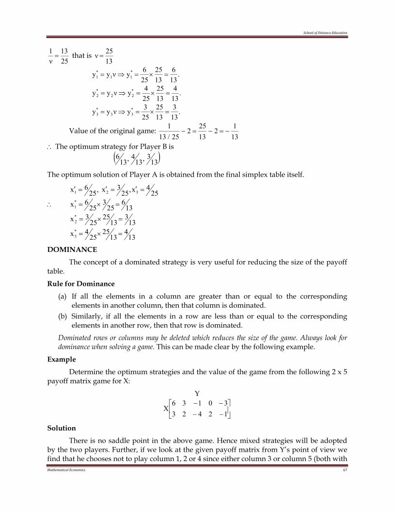
School of Distance Education
Mathematical Economics 67
2513
ν1= that is
1325 ν =
.136
1325
256yνyy *
11*1 =×=⇒=
.134
1325
254yνyy *
22*2 =×=⇒=
.133
1325
253yνyy *
33*3 =×=⇒=
Value of the original game: 131
21325
225/13
1−=−=−
∴ The optimum strategy for Player B is ( )13
3,134,13
6
The optimum solution of Player A is obtained from the final simplex table itself.
254x,25
3x,256x 321 =′=′=′
∴ 136
253
256x*
1 =×=
133
1325
253x*
2 =×=
134
1325
254x*
3 =×=
DOMINANCE
The concept of a dominated strategy is very useful for reducing the size of the payoff table.
Rule for Dominance
(a) If all the elements in a column are greater than or equal to the corresponding elements in another column, then that column is dominated.
(b) Similarly, if all the elements in a row are less than or equal to the corresponding elements in another row, then that row is dominated.
Dominated rows or columns may be deleted which reduces the size of the game. Always look for dominance when solving a game. This can be made clear by the following example.
Example
Determine the optimum strategies and the value of the game from the following 2 x 5 payoff matrix game for X:
Y
⎥⎦
⎤⎢⎣
⎡−−−−
1242330136
X
Solution
There is no saddle point in the above game. Hence mixed strategies will be adopted by the two players. Further, if we look at the given payoff matrix from Y’s point of view we find that he chooses not to play column 1, 2 or 4 since either column 3 or column 5 (both with
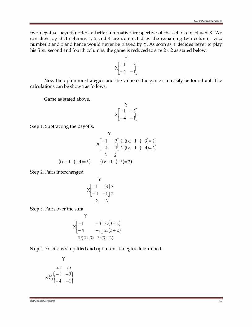
School of Distance Education
Mathematical Economics 68
two negative payoffs) offers a better alternative irrespective of the actions of player X. We can then say that columns 1, 2 and 4 are dominated by the remaining two columns viz., number 3 and 5 and hence would never be played by Y. As soon as Y decides never to play his first, second and fourth columns, the game is reduced to size 2 × 2 as stated below:
Y
⎥⎦
⎤⎢⎣
⎡−−−−
1431
X
Now the optimum strategies and the value of the game can easily be found out. The calculations can be shown as follows:
Game as stated above. Y
⎥⎦
⎤⎢⎣
⎡−−−−
1431
X
Step 1: Subtracting the payoffs.
( )( )( )( )
23341.e.i231.e.i
32
1431
X
Y
=−−−=−−−
⎥⎦
⎤⎢⎣
⎡−−−−
( )( )341.e.i =−−− ( )( )231.e.i =−−−
Step 2. Pairs interchanged
3223
1431
X
Y
⎥⎦
⎤⎢⎣
⎡−−−−
Step 3. Pairs over the sum.
( )( )
)23/(3)32/(223/223/3
1431
X
Y
++
++
⎥⎦
⎤⎢⎣
⎡−−−−
Step 4. Fractions simplified and optimum strategies determined.
⎭⎬⎫
⎩⎨⎧
−−−−
1431
X
Y
5/35/2
5/35/2
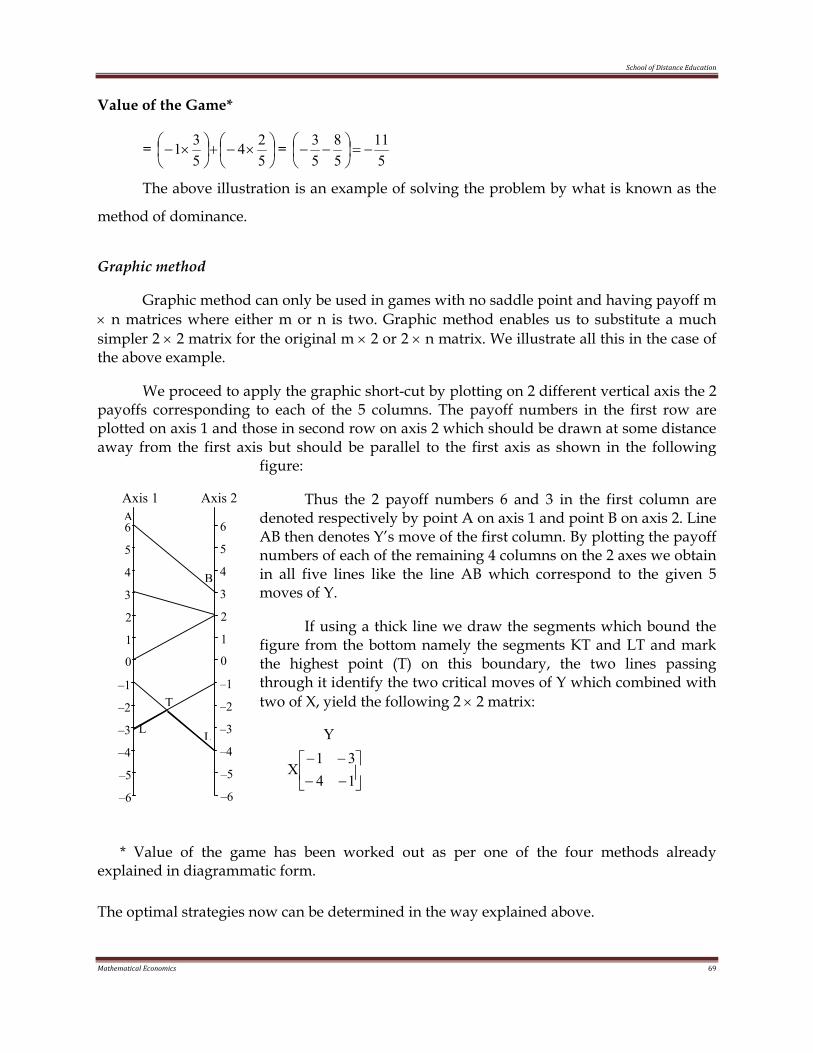
School of Distance Education
Mathematical Economics 69
Value of the Game*
= ⎟⎠⎞
⎜⎝⎛ ×−+⎟
⎠⎞
⎜⎝⎛ ×−
524
531 =
511
58
53
−=⎟⎠⎞
⎜⎝⎛ −−
The above illustration is an example of solving the problem by what is known as the
method of dominance.
Graphic method
Graphic method can only be used in games with no saddle point and having payoff m × n matrices where either m or n is two. Graphic method enables us to substitute a much simpler 2 × 2 matrix for the original m × 2 or 2 × n matrix. We illustrate all this in the case of the above example.
We proceed to apply the graphic short-cut by plotting on 2 different vertical axis the 2 payoffs corresponding to each of the 5 columns. The payoff numbers in the first row are plotted on axis 1 and those in second row on axis 2 which should be drawn at some distance away from the first axis but should be parallel to the first axis as shown in the following
figure:
Thus the 2 payoff numbers 6 and 3 in the first column are denoted respectively by point A on axis 1 and point B on axis 2. Line AB then denotes Y’s move of the first column. By plotting the payoff numbers of each of the remaining 4 columns on the 2 axes we obtain in all five lines like the line AB which correspond to the given 5 moves of Y.
If using a thick line we draw the segments which bound the figure from the bottom namely the segments KT and LT and mark the highest point (T) on this boundary, the two lines passing through it identify the two critical moves of Y which combined with two of X, yield the following 2 × 2 matrix:
⎥⎦
⎤⎢⎣
⎡−−−−
1431
X
Y
* Value of the game has been worked out as per one of the four methods already explained in diagrammatic form.
The optimal strategies now can be determined in the way explained above.
L
Axis 1 Axis 2
1 2 3 4 5 6
0 1
2
3
4
5
6
0
–6 –5 –4 –3 –2 –1
–6
–5
–4
–3
–2
–1
A
B
T
L
School of Distance Education
Mathematical Economics 70
EXERCISES
II. Very Short Answer Questions
1. What is a game?
2. What is a zero sum game?
3. What is saddle point?
4. Define a two person zero sum game.
5. What is a pay-off matrix?
6. What is the use of pay-off matrix in game theory?
III. Short Answer Questions
7. Explain zero sum game and its applications and significance.
8. Discuss theory of games.
9. Explain the usefulness of game theory in economic analysis.
10. Distinguish between a zero sum game and constant sum game.
11. Distinguish between pure strategy game and mixed strategy game.
12. Explain the interrelationship between linear programming and game theory.
13. What are the characteristics based on which the games are classified?
IV. Long Answer Questions
14. Solve the following 2 person zero sum game
⎟⎟⎟
⎠
⎞
⎜⎜⎜
⎝
⎛
442136233
P
15. Solve using dominance property, the game with pay off matrix
A = ⎟⎟⎠
⎞⎜⎜⎝
⎛−
−−105136142
School of Distance Education
Mathematical Economics 71
16. Solve the game with the following payoff matrices.
(i) ⎥⎦
⎤⎢⎣
⎡− 102
31 (ii)
⎥⎥⎥
⎦
⎤
⎢⎢⎢
⎣
⎡
−−
−−
212101212
(iii) ⎥⎥⎥⎥
⎦
⎤
⎢⎢⎢⎢
⎣
⎡
8040042442430423
17. Solve the following games graphically. (i) ⎥⎥⎥
⎦
⎤
⎢⎢⎢
⎣
⎡
2115372
(ii) ⎥⎦
⎤⎢⎣
⎡ −132211
18. Write both the primal and the dual LP problems corresponding to the rectangle games with the following payoff matrices. Solve the game by solving the LP. Problem by simplex method.
(i) ⎥⎥⎥
⎦
⎤
⎢⎢⎢
⎣
⎡
021102210
(ii) ⎥⎥⎥
⎦
⎤
⎢⎢⎢
⎣
⎡
−−
−
226353
311
School of Distance Education
Mathematical Economics 72
Module IV
INPUT-OUTPUT ANALYSIS
UNIT I: INTRODUCTION
The input-output analysis technique was first propounded in 1951 by Prof. W.W. Leontief. The input-output analysis is called as the analysis of inter industry relations. Prof. Leontief gives an explanation to the concept of input-output before launching his technique of input-output analysis. Input implies that object of material which is demanded by the entrepreneur for the purpose of production. Output is the result or outcome of the productive efforts of production. So whatever is sold by a producing firm is output and whatever is purchased by a producing firm is an input. Input gives the cost of production, output gives revenue to the producer.
The input-output analysis tells us that there are industrial inter-relationships and interdependencies in the economic system as a whole. The outputs of one industry are the input of another industry and vice-versa e.g., coal is an input for steel industry and steel is an input for coal industry. We know that agriculture and industry are independent in an economy. In Indian economy, most of our large scale industries are dependent on Agriculture because agriculture provides basic raw material. Agriculture is also dependent on industry because industry provides fertilizer, agriculture implements, machinery etc. Hence these two sectors are quite dependent on each other.
Input-output technique deals with the type of problems, one of which may be described in the following words.
“What level of output should each of the industries produce in an economy so that the total output goal for consumer (That is final consumption) and industrial use (that is intermediate consumption) gets fully satisfied; in other words, consumption equal production, that is all that produced is consumed”.
Input-output analysis is a method of analysis how an industry undertakes production by using the outputs of other industry in the economy and how the output of the given industry is used up in other industries or sectors. Various industries are mutually interdependent. Thus input-output analysis explains the interdependencies of inputs and outputs of various industries in the economy.
Main Features
1. Input-output analysis is concerned with production only. It determines the amounts of different inputs to be used in the production process to get a certain output. Demand theory has no role that is why Baumol calls it as a hard care of input-output analysis. It deals with only technological problems.
2. It is purely an empirical investigation and quite different from theoretical analysis of general equilibrium and as a result, it is both simplified and narrow than the usual general equilibrium theory.
School of Distance Education
Mathematical Economics 73
3. It lays more emphasis on equilibrium phenomenon. It investigates how the various sectors, sub-sectors or industries constituting an economy are interrelated. In Hirschman terminology, industries have both backward and forward linkages and thus are interdependent and with this interdependence of production activities seek to take account of the fact that each industry uses output of other industries as raw materials. According to C.F. Christ, it is like equilibrium theory that is it encompasses all industries and their products. Thus, the input-output analysis technique cannot be applied to the fields of partial equilibrium analysis.
4. This analysis has two parts-first constructing an input output table and second making systematic use of the input-output model
Assumptions of Input-output Analysis – In the construction of a model for any social system, it is inevitable to make certain assumptions. These may not be totally valid but are justifiable to a large extent. They are also necessary to simplify the mathematical aspects.
Following are the assumptions inherent in the model-
1. The economy consists of a number of interacting industries
2. Each industry produces only one good and uses only one process of production.
3. To produce a good the industry requires as input the goods made by other industries, labour and perhaps imports. An industry may use some of its own good. Such use may be considered as a sale to the industry itself.
4. The output of any industry becomes either the input of another industry or the final demand (or the final consumption).
5. In any productive process all inputs are used in fixed proportions and increase input is in proportion with the level of output. Production takes place through processes with constant technical coefficients. The technical coefficient shows the number of units of any industry’s output needed to produce the units of another industry’s output. In other words, it shows the amount of raw materials needed by an industry from any other industry to produce a certain product.
6. All transactions may be considered in terms of money value since money is the suitable common unit for aggregating inputs and outputs of industries. Quantities and prices can also be considered for transactions.
7. In order that the total demand for the product of any industry be just sufficient, we should know the level of output of each industry under consideration.
8. The Isoquant surfaces have been assumed to be having usual convexity that is as we employ more of a factor in product, the output increases at a diminishing rate.
Two Types of Models- Input-output models are of two types: closed in which the entire production is consumed by those participating in the production and open in which some of the production is consumed by external bodies. In the closed model we seek the income of each participant in the system and in the open model to achieve a forecasted demand when the amount of production needed to achieve current demand is known.
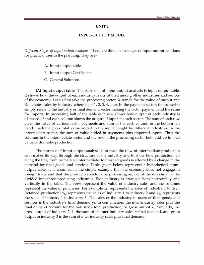
School of Distance Education
Mathematical Economics 74
UNIT 2
INPUT-OUT PUT MODEL
Different Stages of Input-output relations- There are three main stages of input-output relations for practical uses in the planning. They are-
A. Input-output table
B. Input-output Coefficients
C. General Solutions.
(A) Input-output table- The basic tool of input-output analysis is input-output table. It shows how the output of each industry is distributed among other industries and sectors of the economy. Let us first take the processing sector. X stands for the value of output and Xij denotes sales by industry where i, j = 1, 2, 3, 4, ….n. In the payment sector, the subscript simply refers to the industry or final demand sector making the factor payment and the same for imports. In processing half of the table each row shows how output of each industry is disposed of and each column shows the origins of inputs to each sector. The sum of each row gives the value of various factor payments and sum of the each column in the bottom left hand quadrant gives total value added to the input bought by different industries. In the intermediate sector, the sum of value added in payments plus imported inputs. Thus the columns in the intermediate sector and the row in the processing sector both add up to total value of domestic production.
The purpose of input-output analysis is to trace the flow of intermediate production as it makes its way through the structure of the industry and to show how production, all along the line, from primary to intermediate, to finished goods is affected by a change in the demand for final goods and services. Table, given below represents a hypothetical input-output table. It is assumed in the simple example that the economy does not engage in foreign trade and that the productive sector (the processing sector) of the economy can be divided into three producing industries. Each industry is arranged both horizontally and vertically in the table. The rows represent the value of industry sales and the columns represent the value of purchases. For example x11 represents the sales of industry 1 to itself (retained production) x12 represents the sales of industry 1 to industry 2 and x13 represents the sales of industry 1 to industry 3. The sales of the industry to users of final goods and services is the industry’s final demand y1. In combination, the inter-industry sales plus the final demand account for the industry’s total production, or gross output x1. Similarly, the gross output of industry 2, is the sum of its inter industry sales + final demand, and gross output in industry 3 is the sum of inter industry sales plus final demand.
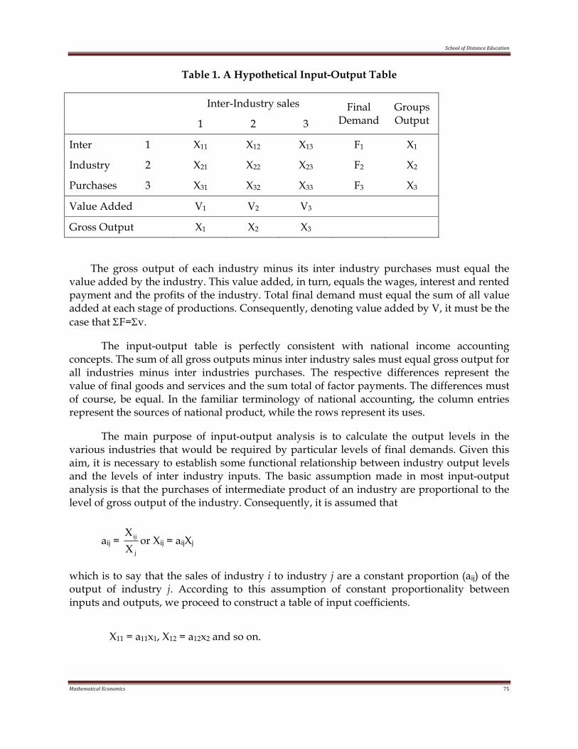
School of Distance Education
Mathematical Economics 75
Table 1. A Hypothetical Input-Output Table
Inter-Industry sales Final Demand
Groups Output 1 2 3
Inter 1 X11 X12 X13 F1 X1
Industry 2 X21 X22 X23 F2 X2
Purchases 3 X31 X32 X33 F3 X3
Value Added V1 V2 V3
Gross Output X1 X2 X3
The gross output of each industry minus its inter industry purchases must equal the value added by the industry. This value added, in turn, equals the wages, interest and rented payment and the profits of the industry. Total final demand must equal the sum of all value added at each stage of productions. Consequently, denoting value added by V, it must be the case that ΣF=Σv.
The input-output table is perfectly consistent with national income accounting concepts. The sum of all gross outputs minus inter industry sales must equal gross output for all industries minus inter industries purchases. The respective differences represent the value of final goods and services and the sum total of factor payments. The differences must of course, be equal. In the familiar terminology of national accounting, the column entries represent the sources of national product, while the rows represent its uses.
The main purpose of input-output analysis is to calculate the output levels in the various industries that would be required by particular levels of final demands. Given this aim, it is necessary to establish some functional relationship between industry output levels and the levels of inter industry inputs. The basic assumption made in most input-output analysis is that the purchases of intermediate product of an industry are proportional to the level of gross output of the industry. Consequently, it is assumed that
aij = j
ij
XX
or Xij = aijXj
which is to say that the sales of industry i to industry j are a constant proportion (aij) of the output of industry j. According to this assumption of constant proportionality between inputs and outputs, we proceed to construct a table of input coefficients.
X11 = a11x1, X12 = a12x2 and so on.
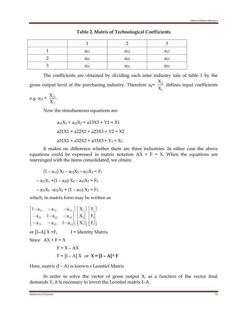
School of Distance Education
Mathematical Economics 76
Table 2. Matrix of Technological Coefficients
1 2 3 1 a11 a12 a13
2 a21 a22 a23
3 a31 a32 a33
The coefficients are obtained by dividing each inter industry sale of table 1 by the
gross output level of the purchasing industry. Therefore aij= j
ij
XX
defines input coefficients
e.g. a12 = 2
12
XX .
Now the simultaneous equations are
a11X1 + a12X2 + a13X3 + Y1 = X1
a21X1 + a22X2 + a23X3 + Y2 = X2
a31X1 + a32X2 + a33X3 + Y3 = X3
It makes no difference whether there are three industries. In either case the above equations could be expressed in matrix notation AX + F = X. When the equations are rearranged with the items consolidated, we obtain.
(1 – a11) X1 – a12X2 – a13X3 = F1
– a21X1 +(1 – a22) X2 – a23X3 = F2
– a31X1 –a32X2 + (1 – a33) X3 = F3
which, in matrix form may be written as
⎥⎥⎥
⎦
⎤
⎢⎢⎢
⎣
⎡
⎥⎥⎥
⎦
⎤
⎢⎢⎢
⎣
⎡
⎥⎥⎥
⎦
⎤
⎢⎢⎢
⎣
⎡
−−−−−−−−−
3
2
1
3
2
1
333231
232221
131211
FFF
XXX
a1aaaa1aaaa1
or [I–A] X =F, I = Identity Matrix
Since AX + F = X
F = X – AX
F = [I – A] X or X = [I – A]-1 F
Here, matrix (I – A) is known s Leontief Matrix
In order to solve the vector of gross output X, as a function of the vector final demands Y, it is necessary to invert the Leontief matrix I–A.
School of Distance Education
Mathematical Economics 77
Uses of Input-output Analysis – Input-Output analysis may have the following uses-
1. Input-output analysis may be used for projection and forecasting purposes. Some planning is used to attain consistency in plans. If a plan lacks consistency, bottlenecks production process may develop and as a result overall growth is affected.
2. Input-output analysis can be used to examine the stimulation process. The stimulation of development is concerned with what is economically feasible, as opposed to forecasting which is concerned with what one expects to happen on the basis of certain set of assumptions.
3. The knowledge of input-output relationships has been found useful in growth and planning exercises of only those countries where manufacturing sector is considerably developed, as a result, there is great interdependence between various productive activities due to lack of considerable backward and forward linkages.
4. The concept of input-output analysis have also some other uses e.g. to forecast import requirement and the balance of payments effects of given changes in final demand, to forecast labour requirements with a given growth target and to forecast investment requirements consistent with a given growth targets, if information is available on incremental capital – output ratio sector by sector.
5. To calculate the matrix multiplier attached to different activities that is direct and indirect effects on the total output of all activities in the system from a unit change in the demand for the output of any one activity.
Limitations of Input-Output Analysis
The input-output analysis has the following limitations-
1. Unrealistic assumptions- The main shortcoming of this analysis is that it is based on unrealistic assumptions of constancy of input coefficient and technique of production.
2. Lack of Substantial Inner-Industry Relations- The less developed countries have typically subsistence economies. Production in the past took place for self consumption. Marketing of goods was quite unimportant. Thus inter industry relations were lacking on a substantial scale.
3. Neglects Economic Efficiency – This analysis neglects the aspects of economic efficiency. It simply analyses as to how outputs are distributed as inputs but this does not imply that resources will be efficient.
4. Limited Scope – The input-output models are of greater use of industrially advanced countries where inter industry transactions are large.
5. No Cost Adjustment – The analysis of cost price relations proceeds on the assumption that each industrial sector adjusts the price of its output by just enough to cover the change in the case of its primary and intermediate output.
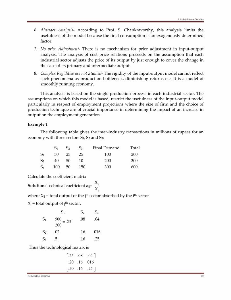
School of Distance Education
Mathematical Economics 78
6. Abstract Analysis- According to Prof. S. Chankravorthy, this analysis limits the usefulness of the model because the final consumption is an exogenously determined factor.
7. No price Adjustment- There is no mechanism for price adjustment in input-output analysis. The analysis of cost price relations proceeds on the assumption that each industrial sector adjusts the price of its output by just enough to cover the change in the case of its primary and intermediate output.
8. Complex Regidities are not Studied- The rigidity of the input-output model cannot reflect such phenomena as production bottleneck, diminishing returns etc. It is a model of smoothly running economy.
This analysis is based on the single production process in each industrial sector. The assumptions on which this model is based, restrict the usefulness of the input-output model particularly in respect of employment projections where the size of firm and the choice of production technique are of crucial importance in determining the impact of an increase in output on the employment generation.
Example 1
The following table gives the inter-industry transactions in millions of rupees for an economy with three sectors S1, S2 and S3:
S1 S2 S3 Final Demand Total S1 50 25 25 100 200 S2 40 50 10 200 300 S3 100 50 150 300 600
Calculate the coefficient matrix
Solution: Technical coefficient aij= j
ij
XX
where Xij = total output of the jth sector absorbed by the ith sector
Xj = total output of jth sector.
S1 S2 S3 S1 25.
200500
= .08 .04
S2 .02 .16 .016 S3 .5 .16 .25
Thus the technological matrix is
⎥⎥⎥
⎦
⎤
⎢⎢⎢
⎣
⎡
25.16.50.016.16.20.04.08.25.
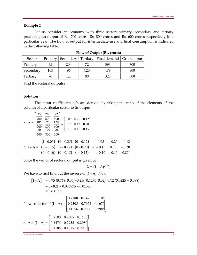
School of Distance Education
Mathematical Economics 79
Example 2
Let us consider an economy with three sectors-primary, secondary and tertiary producing an output of Rs. 700 crores, Rs. 800 crores and Rs. 600 crores respectively in a particular year. The flow of output for intermediate use and final consumption is indicated in the following table.
Flow of Output (Rs. crores) Sector Primary Secondary Tertiary Final demand Gross ouput
Primary 35 200 72 393 700 Secondary 105 96 120 479 800 Tertiary 70 120 90 320 600
Find the sectoral outputs?
Solution
The input coefficients aij’s are derived by taking the ratio of the elements of the column of a particular sector to its output.
∴ A = ⎥⎥⎥
⎦
⎤
⎢⎢⎢
⎣
⎡=
⎥⎥⎥⎥⎥⎥
⎦
⎤
⎢⎢⎢⎢⎢⎢
⎣
⎡
15.015.010.020.012.015.012.025.005.0
60090
800120
70070
600120
80096
700105
60072
800200
70035
∴ I – A = ( ) ( ) ( )( ) ( ) ( )( ) ( ) ( ) ⎥
⎥⎥
⎦
⎤
⎢⎢⎢
⎣
⎡
−−−−−−
=⎥⎥⎥
⎦
⎤
⎢⎢⎢
⎣
⎡
−−−−−−−−−
85.015.010.020.088.015.012.025.095.0
15.0115.0010.0020.0012.0115.0012.0025.0005.01
Since the vector of sectoral output is given by
X = (1 – A)–1 F,
We have to first find out the inverse of (I – A). Now
( )AI− = 0.95 (0.748–0.03)+0.25(–0.1275–0.02)–0.12 (0.0225 + 0.088) = 0.6821 – 0.036875 – 0.01326 = 0.631965
Now co-factor of (I – A) = ⎥⎥⎥
⎦
⎤
⎢⎢⎢
⎣
⎡
7985.02080.01556.01675.07955.02305.01105.01475.07180.0
∴ Adj (I – A) = ⎥⎥⎥
⎦
⎤
⎢⎢⎢
⎣
⎡
7985.01675.01105.02080.07955.01475.01556.02305.07180.0
School of Distance Education
Mathematical Economics 80
∴ (I – A)–1 = ( )( ) 631965.0
1AI
AIAdj=
−−
⎥⎥⎥
⎦
⎤
⎢⎢⎢
⎣
⎡
7985.01675.01105.02080.07955.01475.01556.02305.07180.0
∴ 631965.0
1
XXX
3
2
1
=⎥⎥⎥
⎦
⎤
⎢⎢⎢
⎣
⎡
⎥⎥⎥
⎦
⎤
⎢⎢⎢
⎣
⎡
⎥⎥⎥
⎦
⎤
⎢⎢⎢
⎣
⎡
320479393
7985.01675.01105.02080.07955.01475.01556.02305.07180.0
⎥⎥⎥
⎦
⎤
⎢⎢⎢
⎣
⎡
++++++
=255.52 80.23 43.43
66.56 381.04 57.9749.79 110.41 28.17
631965.01
⎥⎥⎥
⎦
⎤
⎢⎢⎢
⎣
⎡=⎥⎥⎥
⎦
⎤
⎢⎢⎢
⎣
⎡=
600800700
18.37957.50537.442
631965.01
∴ X1 = 700; X2 = 800 and X3 = 600.
These values of Xj’s tally with the sectoral output of X1, X2 and X3 shown in the above table.
The same results can be obtained by Using Cramer’s rule and this is left to the readers as an exercise.
Example 4 In a three sector economy, the input coefficient matrix and final demand vector are as given below:
A = ⎥⎥⎥
⎦
⎤
⎢⎢⎢
⎣
⎡=
⎥⎥⎥
⎦
⎤
⎢⎢⎢
⎣
⎡
600700500
Fand03.02.04.03.01.03.02.03.0
Find the sectoral output X1, X2 and X3 using Cramer’s rule.
Solution: The input-output structure is given by
(I – A) X = F
Now (I – A) = ⎥⎥⎥
⎦
⎤
⎢⎢⎢
⎣
⎡
−−−−−−
13.02.04.07.01.03.02.07.0
∴ ⎥⎥⎥
⎦
⎤
⎢⎢⎢
⎣
⎡
−−−−−−
13.02.04.07.01.03.02.07.0
⎥⎥⎥
⎦
⎤
⎢⎢⎢
⎣
⎡=
⎥⎥⎥
⎦
⎤
⎢⎢⎢
⎣
⎡
600700500
XXX
3
2
1
School of Distance Education
Mathematical Economics 81
Using Cramer’s rule we can solve for X1, X2 and X3 as
X1 = ( )( )
13.02.04.07.01.03.02.07.0
13.06004.07.07003.02.0500
AIAI 1
−−−−−−
−−−−
=−−
= ( ) ( ) ( )( ) ( ) ( )14.003.03.008.01.02.012.07.07.0
4202103.02407002.012.07.0500+−−−+−−−−++−
= 2091319.0
667015.0036.0406.0
189188290==
−−++
Similarly, X2 = ( )( ) 319.0
16002.04.07001.03.05007.0
AIAI 2 −
−−−
=−−
= ( ) ( )319.0
140603.008.01.0500)240700(7.0 +−−−−−+
= 2270319.0
724319.0
2490658==
−+
X3= ( )( ) 319.0
6003.02.07007.01.05002.07.0
AIAI 3 −−
−−
=−−
= ( ) ( ) ( )319.0
14.003.0500140602.02104207.0 +++−++
= 1699319.0
542319.0
8516441==
++
∴ the consistent level of sectoral outputs are X1 = Rs. 2091 crores; X2 = Rs. 2270 crores and X3 = Rs. 1699 crores. The same results can be obtained by using matrix inversion and it is left to the readers as an exercise.
Example 5: In a two industry economy, it is known that industry I uses 10 paise of its own product and 60 paise of commodity II to produce a rupee’ worth of commodity I; industry II uses non of its own product but uses 50 paise of commodity I in producing a rupee’s worth of commodity II and the open sector demands are Rs. 1000 for commodity I and Rs. 2000 for commodity II.
a) Write out the input matrix, the technological matrix and the specific input- output matrix equation for this economy.
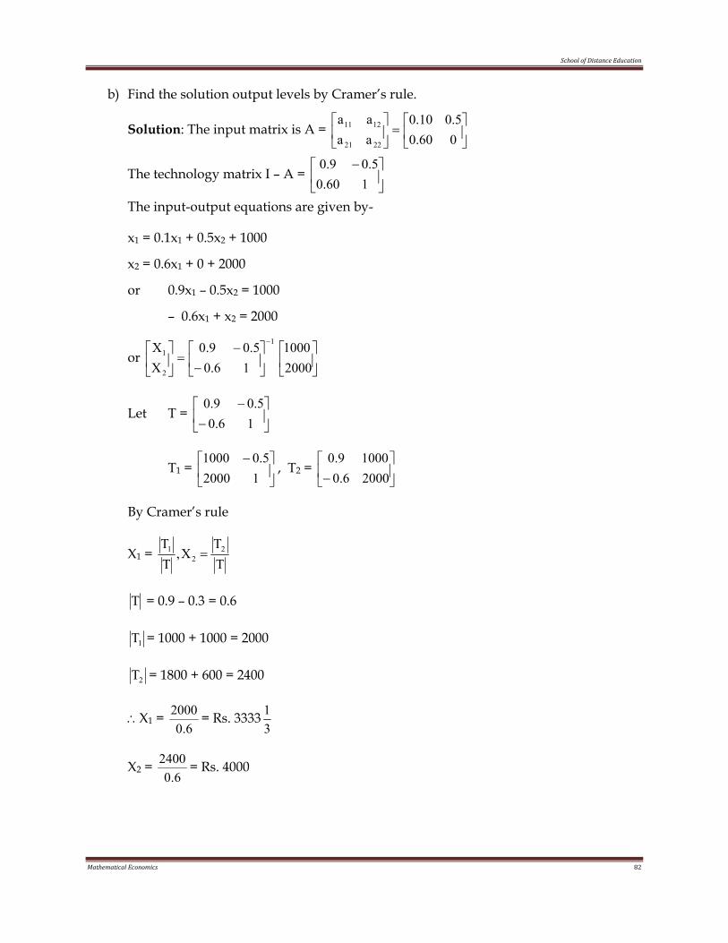
School of Distance Education
Mathematical Economics 82
b) Find the solution output levels by Cramer’s rule.
Solution: The input matrix is A = ⎥⎦
⎤⎢⎣
⎡=⎥
⎦
⎤⎢⎣
⎡060.05.010.0
aaaa
2221
1211
The technology matrix I – A = ⎥⎦
⎤⎢⎣
⎡ −160.0
5.09.0
The input-output equations are given by-
x1 = 0.1x1 + 0.5x2 + 1000
x2 = 0.6x1 + 0 + 2000
or 0.9x1 – 0.5x2 = 1000
– 0.6x1 + x2 = 2000
or ⎥⎦
⎤⎢⎣
⎡⎥⎦
⎤⎢⎣
⎡−
−=⎥
⎦
⎤⎢⎣
⎡−
20001000
16.05.09.0
XX 1
2
1
Let T = ⎥⎦
⎤⎢⎣
⎡−
−16.0
5.09.0
T1 = ⎥⎦
⎤⎢⎣
⎡ −12000
5.01000, T2 = ⎥
⎦
⎤⎢⎣
⎡− 20006.0
10009.0
By Cramer’s rule
X1 = TT
X,TT 2
21 =
T = 0.9 – 0.3 = 0.6
1T = 1000 + 1000 = 2000
2T = 1800 + 600 = 2400
∴X1 = 6.0
2000 = Rs. 333331
X2 = 6.0
2400 = Rs. 4000
School of Distance Education
Mathematical Economics 83
EXERCISES
II. Very Short Answer Questions
1. What is an input-output table? 2. Define Leontieff matrix 3. What are technological coefficients? 4. Give any two uses of input-output model. 5. State two limitations of input-out model.
III. Short Answer Questions
6. What is the input-output technique? Give its nature and assumptions. 7. What is input-output coefficients? What conditions may be filled if they are to be stable
through time? 8. What do you understand by Leontief Inverse Matrix and what does it show? 9. What is input-output analysis? How indispensable it is as a planning technique? Explain. 10. Discuss the significance of input-output table.
IV. Long Answer Questions
11. What are the main purposes (uses) of input-output analysis? 12. Suppose there are two sectors, A, B and the final demand F. The input-output table is
given below: Sectors A B Final Demand Total
A 15 20 45 80
B 5 20 15 40
Primary Input 30 25 5 60
What will be the level of output if the final demand becomes 65 for A and 25 for B? What will happen if final demand (i) doubled, (ii) halved?
13. Explain Leontief input-output model. For a three sector economy the usage, final demand and output corresponding to each sector (in value) is given below:
User S1 S2 S3 Final Demand Output
Producer
S1 80
100
100
40 320
S2 80
200
60 60 400
S3 80
100
100
20 300
School of Distance Education
Mathematical Economics 84
Assuming the technical matrix remain the same, find the output if the final demand
vector changes to ⎥⎥⎥
⎦
⎤
⎢⎢⎢
⎣
⎡
204010
.
14. Solve the following input-output model (I – A) X = F by using Cramer’s rule given.
a. A = ⎥⎥⎥
⎦
⎤
⎢⎢⎢
⎣
⎡=
⎥⎥⎥
⎦
⎤
⎢⎢⎢
⎣
⎡
400500300
F;2.02.01.01.02.004.02.03.0
b. A = ⎥⎥⎥
⎦
⎤
⎢⎢⎢
⎣
⎡=
⎥⎥⎥
⎦
⎤
⎢⎢⎢
⎣
⎡
130012001000
F;0
101
51
101
41
101
41
81
51
15. Find out direct and indirect employment requirement by Cramer’s rule given
A = ⎥⎥⎥
⎦
⎤
⎢⎢⎢
⎣
⎡=
⎥⎥⎥
⎦
⎤
⎢⎢⎢
⎣
⎡=
⎥⎥⎥
⎦
⎤
⎢⎢⎢
⎣
⎡
12.000008.000010.0
L;120150100
F;2.04.01.01.01.03.01.02.02.0