Chapter 4 Sequences and Mathematical Induction. 4.1 Sequences.

General Papers ARKIVOC 2006 (ix) 211-238
ISSN 1424-6376 Page 211 ©ARKAT
Mathematical descriptors of DNA sequences: development and applications
Ashesh Nandy1, Marissa Harle, and Subhash C. Basak*
Natural Resources Research Institute, University of Minnesota, 5013 Miller Trunk Highway,
Duluth, MN 55811, USA 1On leave from Programme in Environmental Science, Jadavpur University, Jadavpur, Kolkata
700032, India E-mail: [email protected]
Abstract Over the last few years several authors have presented various methods to assign mathematical descriptors to DNA sequences in order to quantitatively compare the sequences and determine similarities and dissimilarities between them. The plethora of different methods used have made it necessary to compare them and determine which one(s), if any, best meet the needs required to characterize DNA sequences. With the very rapid rise in available DNA sequence data and the strong need for robust quantitative techniques to determine regions of interest in these sequences, numerical characterization of DNA and RNA sequences will be of great importance in filling a part of this need. Keywords: Graphical representation, numerical characterization, mathematical descriptors, DNA sequences
Contents 1. Introduction 2. Structure-Property Similarity Principle 3. Graphical Representations 3.1 Different graphical methods 3.2 Problems and prospects 4. Numerical Characterization 4.1 The goals 4.2 Different approaches 4.3 Comparative analysis 5. Conclusion: The Road Ahead

General Papers ARKIVOC 2006 (ix) 211-238
ISSN 1424-6376 Page 212 ©ARKAT
1. Introduction The stupendous growth in the DNA sequence data over the last few years – amounting to over 100 billion bases in the DNA sequence databanks by 2005 – necessitates mathematical techniques to analyze them for extraction of relevant information rapidly and accurately. While statistical methods based on nucleotide frequencies and identification of motifs such as promoter sequences have remained the staple tools for analysis of gene sequences, there have been several recent attempts to mathematically characterize sequence segments to identify regions of biological interest. The basic idea behind numerical characterization is that specific gene sequences are generally unique and therefore possess a characteristic signature in the composition and distribution of the nucleotides that make up the genes. The departure from uniqueness will come from mutations although some degree of homology will be maintained. Numerical characterization will seek to capture the essence of this homology so that each gene can be characterized by one number or a vector that identifies a gene. The same construct can be applied to significant regio-specific motifs that may be identified within the gene, corresponding to, say, particular structural aspects of the downstream protein or enzyme, or within a DNA or RNA sequence segments such as promoter sequences. In a broader perspective, numerical characterization can play an important role in the identification of coding segments in newly emerging sequences, or prediction of functions from sequences. The primary step in creating a mathematical descriptor is to develop reliable techniques for characterizing DNA/RNA sequences. While algorithms can be constructed to generate mathematical representations directly from DNA primary sequences, it is intuitively more appealing to represent a long DNA sequence in the form of a graph and visually identify regions of interest or the distribution of bases along the sequence. Most methods that have been proposed in the literature to numerically characterize DNA sequences are based on one or more graphical representations of such sequences, and several applications have been made using these techniques. This is a new field of enquiry and has been gathering momentum over the last decade. In this review we focus on the different mathematical techniques for characterizing DNA sequences. We briefly enumerate the graphical representations of DNA sequences that form the foundations of these numerical techniques, and then discuss the techniques themselves. We propose a set of criteria of what the numerical descriptors are supposed to achieve, and then compare the different methods on the basis of the results they have demonstrated for a set of gene sequences measured against the corresponding amino acid sequences. We hope that this will highlight both the utilities and limitations of the current crop of numerical methods and thus lead the way towards more sophisticated analysis and improvements in techniques for better understanding of what information the DNA sequences contain and how numerical techniques can help. Mathematical descriptors of DNA sequences and their use in rationalizing biological properties of DNA follow from the structure-property similarity principle.
General Papers ARKIVOC 2006 (ix) 211-238
ISSN 1424-6376 Page 213 ©ARKAT
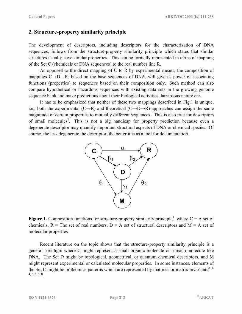
2. Structure-property similarity principle The development of descriptors, including descriptors for the characterization of DNA sequences, follows from the structure-property similarity principle which states that similar structures usually have similar properties. This can be formally represented in terms of mapping of the Set C (chemicals or DNA sequences) to the real number line R. As opposed to the direct mapping of C to R by experimental means, the composition of mappings C→D→R, based on the base sequences of DNA, will give us power of associating functions (properties) to sequences based on their composition only. Such method can also compare hypothetical or hazardous sequences with existing data sets in the growing genome sequence bank and make predictions about their biological activities, hazardous nature etc. It has to be emphasized that neither of these two mappings described in Fig.1 is unique, i.e., both the experimental (C→R) and theoretical (C→D→R) approaches can assign the same magnitude of certain properties to mutually different sequences. This is also true for descriptors of small molecules1. This is not a big handicap for property prediction because even a degenerate descriptor may quantify important structural aspects of DNA or chemical species. Of course, the less degenerate the descriptor, the better it is as a tool for documentation.
C R
D
M
α
β1 β2
θ1 θ2γ1
Figure 1. Composition functions for structure-property similarity principle1, where C = A set of chemicals, R = The set of real numbers, D = A set of structural descriptors and M = A set of molecular properties Recent literature on the topic shows that the structure-property similarity principle is a general paradigm where C might represent a small organic molecule or a macromolecule like DNA. The Set D might be topological, geometrical, or quantum chemical descriptors, and M might represent experimental or calculated molecular properties. In some instances, elements of the Set C might be proteomics patterns which are represented by matrices or matrix invariants2, 3,
4, 5, 6, 7, 8.
General Papers ARKIVOC 2006 (ix) 211-238
ISSN 1424-6376 Page 214 ©ARKAT
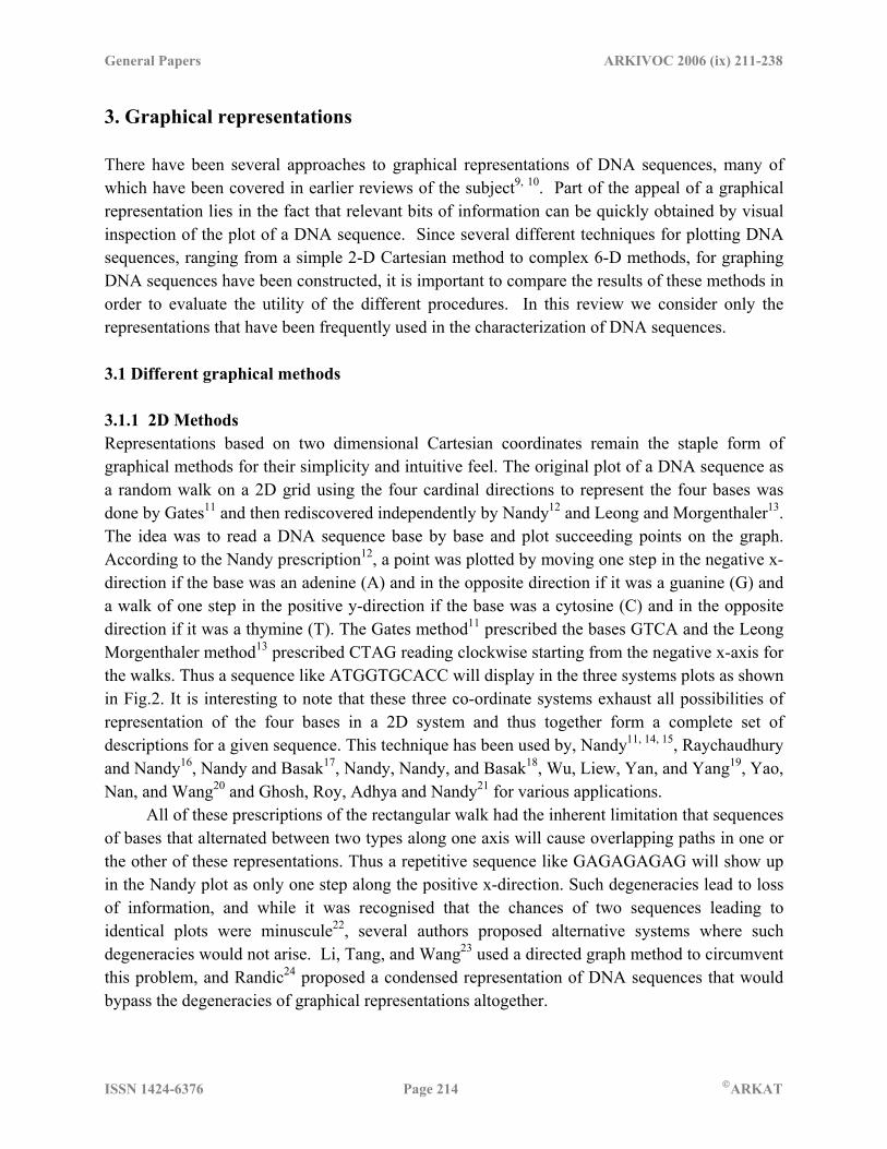
3. Graphical representations There have been several approaches to graphical representations of DNA sequences, many of which have been covered in earlier reviews of the subject9, 10. Part of the appeal of a graphical representation lies in the fact that relevant bits of information can be quickly obtained by visual inspection of the plot of a DNA sequence. Since several different techniques for plotting DNA sequences, ranging from a simple 2-D Cartesian method to complex 6-D methods, for graphing DNA sequences have been constructed, it is important to compare the results of these methods in order to evaluate the utility of the different procedures. In this review we consider only the representations that have been frequently used in the characterization of DNA sequences. 3.1 Different graphical methods 3.1.1 2D Methods Representations based on two dimensional Cartesian coordinates remain the staple form of graphical methods for their simplicity and intuitive feel. The original plot of a DNA sequence as a random walk on a 2D grid using the four cardinal directions to represent the four bases was done by Gates11 and then rediscovered independently by Nandy12 and Leong and Morgenthaler13. The idea was to read a DNA sequence base by base and plot succeeding points on the graph. According to the Nandy prescription12, a point was plotted by moving one step in the negative x-direction if the base was an adenine (A) and in the opposite direction if it was a guanine (G) and a walk of one step in the positive y-direction if the base was a cytosine (C) and in the opposite direction if it was a thymine (T). The Gates method11 prescribed the bases GTCA and the Leong Morgenthaler method13 prescribed CTAG reading clockwise starting from the negative x-axis for the walks. Thus a sequence like ATGGTGCACC will display in the three systems plots as shown in Fig.2. It is interesting to note that these three co-ordinate systems exhaust all possibilities of representation of the four bases in a 2D system and thus together form a complete set of descriptions for a given sequence. This technique has been used by, Nandy11, 14, 15, Raychaudhury and Nandy16, Nandy and Basak17, Nandy, Nandy, and Basak18, Wu, Liew, Yan, and Yang19, Yao, Nan, and Wang20 and Ghosh, Roy, Adhya and Nandy21 for various applications. All of these prescriptions of the rectangular walk had the inherent limitation that sequences of bases that alternated between two types along one axis will cause overlapping paths in one or the other of these representations. Thus a repetitive sequence like GAGAGAGAG will show up in the Nandy plot as only one step along the positive x-direction. Such degeneracies lead to loss of information, and while it was recognised that the chances of two sequences leading to identical plots were minuscule22, several authors proposed alternative systems where such degeneracies would not arise. Li, Tang, and Wang23 used a directed graph method to circumvent this problem, and Randic24 proposed a condensed representation of DNA sequences that would bypass the degeneracies of graphical representations altogether.
General Papers ARKIVOC 2006 (ix) 211-238
ISSN 1424-6376 Page 215 ©ARKAT
Gates Nandy Leong and Morgenthaler
A
C G
T
A
C
G
T
A
C
G
T
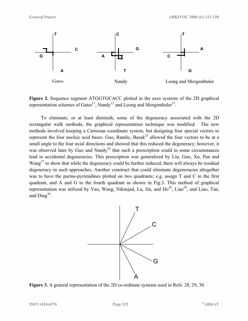
Figure 2. Sequence segment ATGGTGCACC plotted in the axes systems of the 2D graphical representation schemes of Gates11, Nandy12 and Leong and Morgenthaler13. To eliminate, or at least diminish, some of the degeneracy associated with the 2D rectangular walk methods, the graphical representation technique was modified. The new methods involved keeping a Cartesian coordinate system, but designing four special vectors to represent the four nucleic acid bases. Guo, Randic, Basak25 allowed the four vectors to be at a small angle to the four axial directions and showed that this reduced the degeneracy; however, it was observed later by Guo and Nandy26 that such a prescription could in some circumstances lead to accidental degeneracies. This prescription was generalized by Liu, Guo, Xu, Pan and Wang27 to show that while the degeneracy could be further reduced, there will always be residual degeneracy in such approaches. Another construct that could eliminate degeneracies altogether was to have the purine-pyrimidines plotted on two quadrants; e.g. assign T and C to the first quadrant, and A and G to the fourth quadrant as shown in Fig.3. This method of graphical representation was utilized by Yau, Wang, Niknejad, Lu, Jin, and Ho28, Liao29, and Liao, Tan, and Ding30.
C
T
G
A Figure 3. A general representation of the 2D co-ordinate systems used in Refs. 28, 29, 30.

General Papers ARKIVOC 2006 (ix) 211-238
ISSN 1424-6376 Page 216 ©ARKAT
The aim of avoiding degeneracies was followed up by He and Wang31 by dividing the four nucleic acid bases in a sequence into their structural groups. Division was based upon the purine (R=A,G), pyrimidine (Y=C,T), amino (M=A,C), keto (K=T,G), and weak H-bond (W=A,T), and strong H-bond (S=C,G). Each DNA sequence is plotted on these characteristic coordinates and the graphs were called characteristic graphs. This method eliminates degeneracy and also helps with visual inspection of the different structural features and bonds in a sequence. Taking our sample sequence ATGGTGCACC again, the technique will generate graphs like that in Fig.4. We show only two out of the twelve possible graphs. This method was extended and subsequently used by Song and Tang32 among others.
A T G G T G C A C C
A
G
Y
A T G G T G C A C C
C
R
T
a b
Figure 4a and 4b. The 2D characteristic pyrimidine (3a) and purine (3b) curves of the first 10 bases (ATGGTGCACC) in the human beta globin gene as proposed by Song and Tang32 (Ref. 32). A different 2D approach that doesn’t involve the Cartesian coordinate system was also used for graphical representation. Four horizontal lines are drawn on a surface and labelled A, G, T, and C. Then the bases of the DNA sequence of interest are placed horizontally, one unit distance apart, along the bottom of the four lines. For each base in the sequence, a dot is placed along the appropriate horizontal line and all the dots are connected at the end. This method is useful in that there is no degeneracy involved. Thus, a sequence such as ATGGTGCACC will have a graph such as shown in Fig.5. Since the four horizontal lines can be labelled in any order, there will be 4! = 24 possible graphs associated with each DNA sequence. Among those to use this method include Randic, Vracko, Lers and Plavsic33, 34 and Yau, Liao and Wang35 who used the technique to analyse RNA secondary structures.

General Papers ARKIVOC 2006 (ix) 211-238
ISSN 1424-6376 Page 217 ©ARKAT
A T C
G A C A C T CG G T G
Figure 5. The 2D “four horizontal line” curve of the first 10 bases (ATGGTGCACC) in the human beta globin gene in the representation proposed by Ref. 33 and Ref. 34. Graphical representation can also be done by using a binary method. The four bases are split into their three classifications, amino(M)/keto(K), purine(R)/pyrimidine(Y), and weak(W)/strong(S). Then, a value of 1 is ascribed to a R, M, or W type of base in the sequence, and value of 0 is ascribed to a Y, K, or S type of base in the sequence. The graphing is done by placing two horizontal lines, each labelled with a 1 or a 0, one unit distance apart. The binary sequence is then placed along the bottom of the horizontal lines with each number being separated by one unit distance. For each number in the sequence, a dot is place on the corresponding horizontal line, and the dots are connected. There will be three of these characteristic graphs for each DNA sequence at hand. Thus, a sequence such as ATGGTGCACC will have 3 graphs such as the ones shown in Fig. 6. Among those to use this method were Li and Wang36, Liao and Wang37, Liao and Ding38, and Wang and Zhang39.
0
1
0
1
0
1
1 0 001 01 11 0
1 0 010 00 10 0
1 1 000 10 10 0
R, Y
M, K
W, S
Figure 6. The 2D “two horizontal line” curves of the first 10 bases (ATGGTGCACC) in the human beta globin gene (Refs. 36, 39). Another graphical method proposes the novel idea of utilizing square units called cells. The novel cell design involves a unit square in which the four points in the corners are designated as the four bases A, T, C, and G (Fig.7a). The x-coordinate of the base in the unit cell

General Papers ARKIVOC 2006 (ix) 211-238
ISSN 1424-6376 Page 218 ©ARKAT
is obtained by finding which column the individual base is in. By labelling the first column as zero, the even columns are found by the formula (2(i-1)) and the odd columns are found by ((2(i-1))+1) where i is the base number. Then the y-coordinate is found by whether the base is in the first row or the second row of the cell. In summary, the following designations are given to each base: (2(i-1), 0) = G, (2(i-1), 1) = A, (2(i-1)+1, 0) = C, and (2(i-1)+1, 1) = T where i is the position of the base in the sequence. Then a sequence such as ATGGTGCACC will have a graph such as the one in Fig.7b. This methodology was used by Yao and Wang40.
A
C G
T
Figure 7a. Representation of a cell.
T A GG GT AC C C
Figure 7b. The 2D cell method of Yao and Wang40 showing the plot of the first 10 bases (ATGGTGCACC) in the human beta globin gene.
A slightly different graphical approach involves making a “worm” curve41. This method is useful in that it avoids intersection of the curve with itself, and it uses a smaller amount of space than other methods. The amount of space needed to graph a DNA sequence is approximately equal to √n, where n is the number of bases in the sequence41. Therefore, if the sequence has 3600 nucleic acid bases, graphing can be done in a 60 x 60 square grid. Each base is assigned to a set of numbers; A = 0 0, G = 0 1, C = 1 0, T = 1 1, and the sequence is rewritten with the appropriate digits in place of each base. Graphing involves a series of connecting vertical and horizontal lines where each vertical line represents a nucleic acid base and every horizontal line represents the bond connecting the bases41. A 900 turn is made at every site if the move doesn’t bring you to a site that has already been visited, otherwise a left (2700) turn will be made41. For example, by looking at Fig.8, the first base in the sequence is A(0,0) so a vertical line one unit distance in length is placed starting at the center of the grid. Its starting and ending points are labelled with a 0 and a 0 respectively. Then a horizontal line is drawn at a 900 angle and a vertical line representing T(1,1) is drawn in with its starting and ending points labelled. Since a 900 turn would lead to a site already visited, a 2700 turn is made and a vertical line representing G is made. When the curve is finished, a dot is placed on the corners that represent a 1, leaving the blank spots to be represented by a 0. This method was used by Randic, Vracko, Zupan, and

General Papers ARKIVOC 2006 (ix) 211-238
ISSN 1424-6376 Page 219 ©ARKAT
Novic41 and Randic42. Fig.8 shows a plot of the sequence ATGGTGCACC in this representation. Note that some corners are not marked as dictated by the algorithm.
Figure 8. The first 10 bases (ATGGTGCACC) of the human beta globin gene represented by the “worm curve.” This representation is used in Refs. 41 and 42. In another form of graphical representation43 a square is drawn with the four corners labelled with the four nucleic acid bases. The first base in the sequence at hand is assigned to the location half way between the center of the square and the corner of the square to which the base belongs. The next base in the sequence will be placed half way between the location of the first base and the corner of the square to which it belongs. In summary, each base in the sequence will be placed half way between the position of the preceding base and the corner of the square to which it belongs. This type of representation was done originally by Jeffrey44 and later by Randic and Zupan43 in connection with expansion of the scope of visual representations. 3.1.2 3D Graphical representation A 3D graphical representation for DNA sequences was originally proposed by Hamori and his group (see, e.g. Ref 45), with the aim of facilitating numerical characterization of DNA sequences. A different 3D representation was devised by Randic, Vracko, Nandy, and Basak46,
extending the 2D methods to a 3D graph involved assigning each of the four bases to the corners of a regular tetrahedron. The bases are assigned as follows; A(+1, -1, -1), G(-1, +1, -1), C(-1, -1, +1), and T(+1, +1, +1). The graph is then plotted by placing the first base in the sequence at its correct position; say the first base was an A so its position would be (+1, -1, -1). Then if the next base is a T, it would be placed at (+2, 0, 0). The placement of any base in the sequence will depend on the position of the preceding base in the sequence. This method and its variations were used by Randic, Vracko, Nandy, and Basak46, Li and Wang47, and Yao, Nan, and Wang48.

General Papers ARKIVOC 2006 (ix) 211-238
ISSN 1424-6376 Page 220 ©ARKAT
A widely used 3D method of graphical representation was done by first assigning the x and y axis values to the four bases: A to the negative x-axis, G to the positive x-axis, T to the negative y-axis, and C to the positive y-axis. The z-axis value was the number of time that particular base was repeated in the DNA sequence at hand. Thus, the z values for the sequence ATGGTGCACC will be as follows: 1, 1, 1, 2, 2, 3, 1, 2, 2, 3. The points of each base in the sequence are placed in 3D space and a line connects the points. This method and its variations were used by Yuan, Liao, and Wang49, Liao and Wang50, Liao, Zhang, Ding, and Wang51, Zu, Liao, and Ding52, and Bai, Zhu, and Wang53. 3.1.3 4D Graphical representation Instead of using a 2D or 3D method, Chi and Ding54 used a technique involving a novel 4D numerical representation of a DNA sequence. The advantage of a 4D representation is the avoidance of overlapping and intersecting of the DNA curve with itself. The disadvantage of this method is that the graphical visualization and the ability to directly compare two DNA sequences is lost, which are the advantages of 2D and 3D methods. The idea behind this approach is to obtain the 4D coordinates of the DNA sequence based on the three classifications of DNA bases. It is known that the four nucleic acids A, T, G, and C can be separated on the basis of the distributions of purine-pyrimidine (R/Y), amino-keto (M/K), and weak-strong (W/S) bonds. The classifications are as follows: R=(A, G) and Y=(C, T), M=(A, C) and K=(G, T), W=(A, T) and S=(C, G). A binary technique assigned the value of 1 to Y, K, and S and 0 to R, M, and W. Letting R/Y, M/K, and W/S represent the first three coordinates respectively, the fourth coordinate (i) is represented by the position of the base in the DNA sequence. Therefore, the following assignments were made for the four bases: A(0,0,0,i), G(0,1,1,i), C(1,0,1,i), and T(1,1,0,i). There are 23=8 different arrangements of R/Y, M/K, and W/S with {0, 1}, and the 8 arrangements are as follows: I{R,M,W}, II{R,M,S}, III{R,K,W}, IV{R,K,S}, V{Y,M,W}, VI{Y,M,S}, VII{Y,K,W}, VIII{Y,K,S}. Symmetry exists among the arrangements I and VIII, II and VII, III and VI, IV and V. The four vertices of a regular tetrahedron are obtained when the four coordinates are projected along the fourth coordinate to 3D space. This 4D representation is unique since symmetry and rotation do not change the curve. 3.1.4 Other graphical representations Several other techniques of representations of DNA sequences have been proposed by different authors. Liao and Wang55 proposed a 6-dimensional representation, while Randic, Lers, Plavsic, Basak, and Balaban56 proposed a novel four-color map representation. In this latter method, a sequence of spiralling unit squares is drawn and the first base in the sequence is placed in the centre of the spiral. The rest of the bases in the sequence then spiral clockwise around this first base. After the last base has been placed, the map is sectioned off according to the four bases and each base is given one color. By graphing in this manner, it is possible to see regions in the map belonging to one particular base and thus get an idea of base distribution.

General Papers ARKIVOC 2006 (ix) 211-238
ISSN 1424-6376 Page 221 ©ARKAT
3.2 Problems and prospects The above methods provide almost a complete picture of the graphical representation techniques of DNA sequences and techniques to mathematically characterize the underlying sequences. All methods that require plotting systems in four dimensions and above are difficult to visualize, and even the usefulness of a 3D system to comprehend the base distribution is open to question. On the other hand, 2D methods that do not exclude repetitive walks necessarily lose some amount of information, while those that do completely meet requirements of non-degeneracy have not yet been used to demonstrate any identifiable and useful visual clues to DNA or gene properties. For visual techniques to play any important role in the biologist’s quest for data mining from the libraries of DNA sequences, these methods need to be applied to different problems where the visual clues will play crucial roles and thus determine the most useful ones among them. 4. Numerical characterization 4.1 The goals The idea behind numerical characterization of a DNA sequence is to devise mathematical descriptors that would capture the essence of the base composition and distribution of the sequence in a quantitative manner which would facilitate sequence identification and comparison of similarities and dissimilarities of sequences. Base composition provides gross information of the total content of each base in the sequence and is easily determined. Base distribution is more informative and capable of differentiating among various genes and species even if the base composition numbers are identical as is the case with highly conserved genes like histone H4 or many mutational variations of viral genes. It is expected that since the sequence of a gene is almost unique in the DNA of a species, and bears close homology with the same gene of other species, but are quite different from other genes, the base composition and distribution characteristics would form part of a set of descriptors which can quantify each gene sequence. The objective of the numerical characterizations methods for DNA sequences proposed by several authors is to devise a number that would describe the base distribution. Testing of the efficiency of the mathematical descriptors has been done with the first exon of the DNA sequence of the beta globin gene, comparing the sequences from different species for their similarities and dissimilarities. In this review we examine critically the methods and published results using the mathematical descriptors to determine which method or methods generate the best results.
General Papers ARKIVOC 2006 (ix) 211-238
ISSN 1424-6376 Page 222 ©ARKAT
4.2 Different approaches 4.2.1 Geometrical method There have been two approaches to define such descriptors – geometrical, and graph-theoretical. The geometrical approach, done first by Raychaudhury and Nandy16, is derived from the graphical representation of DNA sequences on a 2D rectangular grid using the (x,y) co-ordinate representation of each base in the sequence as the numerical equivalent. Next, first order moments (µx,µy) and a graph radius (gR) are defined for each sequence by the formulae
Nxi
xΣ
=µ , Nyi
yΣ
=µ and 22yxRg µµ +=
where the (xi, yi) represent the co-ordinates of each point on the plot and N is the total number of the bases in the segment. The gR here represents the Base Distribution index and is critically dependent upon the position of each base in the sequence. The definition of the gR and the first order moments also enables computation of graph similarity/dissimilarity index defined as
221
221 )()( yyxxRg µµµµ −+−=∆
where the µ1 and µ2 refer to two different DNA sequences. The gR and the ∆gR have been found to be very sensitive measures of the sequence composition and distribution16,17,18, the values depending on the type of mutations and where in the sequence they are. gR is specially useful in comparing equal length sequences22. 4.2.2 Graph-theoretical method In the graph-theoretical approach, a DNA sequence is represented by an embedded graph G = [V, R], where V is the nonempty set of vertices {consisting of individual bases (A, T, G, C)} of the graph G and R is the binary relation. For any pair (i,j) of vertices (bases) in the sequence, (i, j)∈ R, they are either connected (adjacent) or not. Such a graph may be represented by an adjacency matrix A = {aij} where
aij = 1, if i and j are connected aij = 0, otherwise A graph theoretic distance matrix D can be formulated as Dij = (dij), where dij is the number of edges between vertices i and j in the embedded graph. A large number of graph invariants have been formulated based on different types of matrices57, 58. One particular matrix, the D
D matrix
and its leading eigenvalue, have been used to quantify shapes of graphs59. The elements of the DE/DG matrix is (dE/dG)ij, where dE represents the Euclidean distance between vertices i and j, whereas dG is the graph theoretical (topological) distance between the vertex pair (i, j). Such distance/distance (DE/DG, or D/D for short) matrices could be directly computed for their eigenvalues. However, because Euclidean distances are always equal to or less than the graph-theoretical distances by construction, the matrix elements were raised to high powers until all elements <1 vanished leaving only the unit ratios from which the leading eigenvalues could be easily computed. Following the initial paper of Randic, Vracko, Nandy and Basak46 showing

General Papers ARKIVOC 2006 (ix) 211-238
ISSN 1424-6376 Page 223 ©ARKAT
the applicability of this technique, leading eigenvalues of the D/D and associated matrices have been considered to be good descriptors of DNA sequences. The availability of leading eigenvectors computed in this manner enabled an easy comparison of DNA sequences for their sequence similarity or dissimilarity. In the simple approach, where one leading eigenvalue was used to characterize a sequence, the differences between the eigenvalues were taken to be an index of sequence similarity/dissimilarity. In the graphical approaches where more than one graph was indicated to completely represent a sequence, a set of leading eigenvalues was generated, one associated with each representation, and the complete set was taken to be the numerical characterization of the sequence (see e.g. Song and Tang32). Differences between sequences were computed by assuming that each set of n leading eigenvalues represented a n-dimensional vector where each member of the set represented a component of the vector. Next, computing the distance between the end-points of the vectors, two sequences would be considered relatively similar if this end-distance was small, and relatively dissimilar if the end points were far apart. The same arguments could be applied in relation to the angle between the relevant vectors – two sequences are very similar if the angle between the two vectors was close to zero and relatively dissimilar otherwise. The arguments would be carried farther when more than two sequences were available by considering the hierarchy of the distance measures (see e.g. He and Wang60). The initial developments in characterizing DNA sequences using matrix methods were by Randic and Vracko61 and Randic, Vracko, Nandy and Basak46 where they used 2D and 3D graphical representation of DNA sequences to generate descriptor matrices. The technique can be most easily understood by considering a 2D projection of the 3D geometry of their graphical representation. Consider, for example, the plot of ATGGTGCACC in the Nandy representation (Fig. 9). The graph theoretic distances are seen in blue and the Euclidean distances in red (unless overlapping). The D/D matrix elements based on this graph are given in Table 1 for the first 5 bases. The two papers referred give a detailed workout of the results for the first exon of the human beta globin gene.
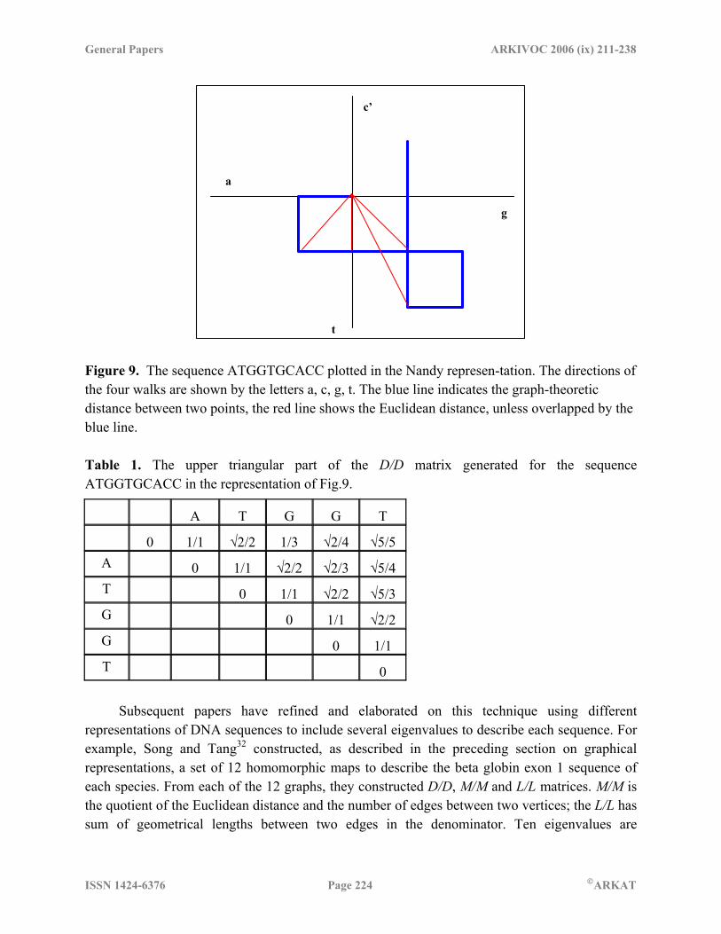
General Papers ARKIVOC 2006 (ix) 211-238
ISSN 1424-6376 Page 224 ©ARKAT
c’
a
g
t Figure 9. The sequence ATGGTGCACC plotted in the Nandy represen-tation. The directions of the four walks are shown by the letters a, c, g, t. The blue line indicates the graph-theoretic distance between two points, the red line shows the Euclidean distance, unless overlapped by the blue line. Table 1. The upper triangular part of the D/D matrix generated for the sequence ATGGTGCACC in the representation of Fig.9.
A T G G T 0 1/1 √2/2 1/3 √2/4 √5/5
A 0 1/1 √2/2 √2/3 √5/4 T 0 1/1 √2/2 √5/3 G 0 1/1 √2/2 G 0 1/1 T 0
Subsequent papers have refined and elaborated on this technique using different representations of DNA sequences to include several eigenvalues to describe each sequence. For example, Song and Tang32 constructed, as described in the preceding section on graphical representations, a set of 12 homomorphic maps to describe the beta globin exon 1 sequence of each species. From each of the 12 graphs, they constructed D/D, M/M and L/L matrices. M/M is the quotient of the Euclidean distance and the number of edges between two vertices; the L/L has sum of geometrical lengths between two edges in the denominator. Ten eigenvalues are

General Papers ARKIVOC 2006 (ix) 211-238
ISSN 1424-6376 Page 225 ©ARKAT
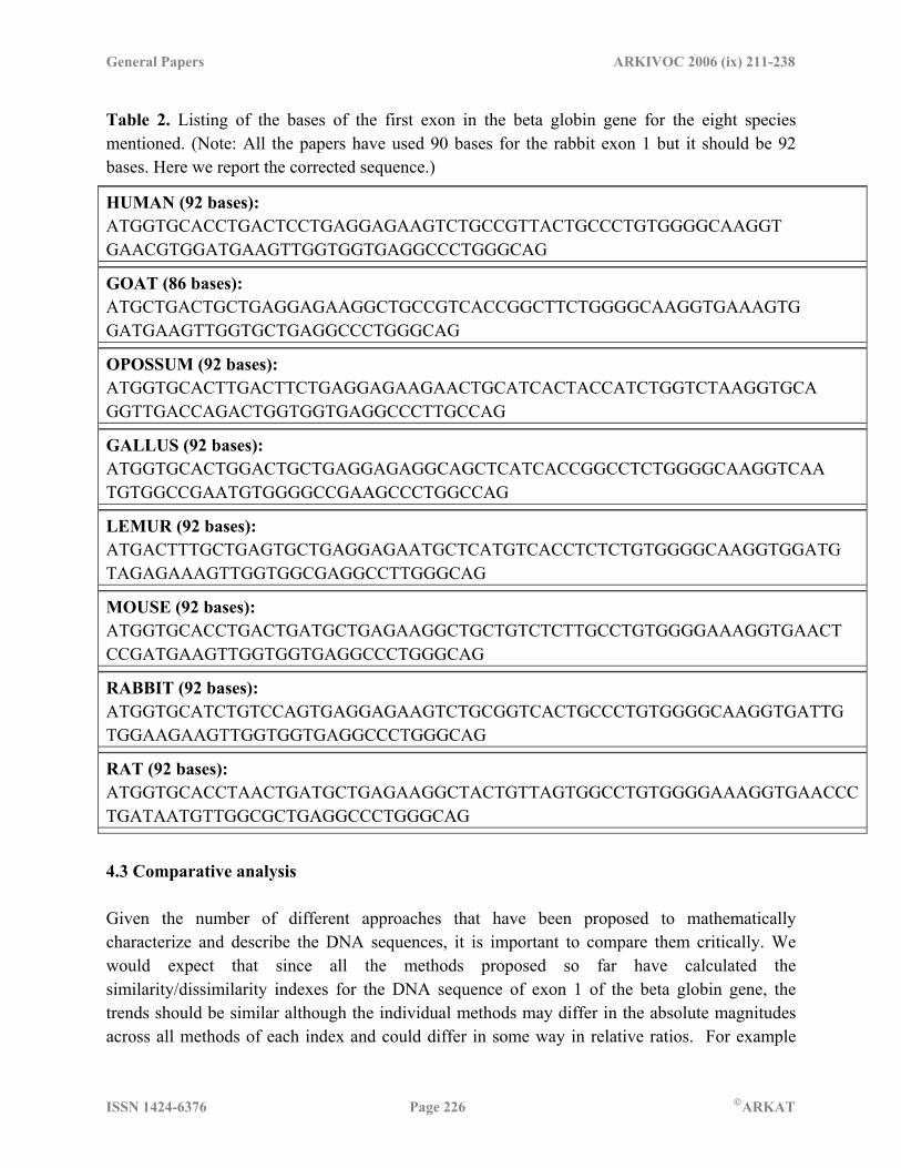
computed for the AYG curve and compared with the D/D values based on the 2D representation of Nandy12. From a comparison of L/L eigenvalues trends with D/D values they conclude that the two approaches lead to similar results and that a few leading eigenvalues is sufficient to characterize DNA sequences. In a slightly different model, He and Wang60 also derived from frequencies of triplets in a binary representation of DNA sequences based on their structural and other properties 24-component descriptors of each beta globin exon 1 sequence from which they computed the distance between any two pairs of the sequences of 8 species of animals. In the same paper they also constructed 6-component vectors made up from leading eigenvalues of condensed matrices derived by them from the DNA sequences and proceeded to compare the same set of 8 sequences with essentially similar results to their 24-component derivation. Table 2 lists the sequences of the first exons of the beta globin genes of various species used by the different authors. In other examples of using novel approaches to formulate numerical characterization of DNA sequences, we may mention the 12-component vector approach of Randic, Vracko, Lers and Plavsic34 constructed with normalized leading eigenvalues from a four horizontal line graphing method, a 16-component vector approach from a consideration of the frequency of occurrence of all possible ordered pairs of adjacent bases (Randic24) and a 64-component vector approach from analysis of frequency of occurrence of all ordered triplets of bases (Randic, Guo, Basak62). Li and Wang36 based their technique on the binary coded characteristic curves representation of DNA sequences of He and Wang60 discussed above and constructed 3-component vectors from sums of maximal and minimal eigenvalues of the three L/L matrices corresponding to the three characteristic sequences. Liao and Wang37 used a simplified 3-component vector approach from sets of characteristic curves constructed from DNA sequences with the bases taken pair wise on the basis of their structural and chemical properties: purine(A,G)/pyrimidine(C,T), amino(A,C)/keto(G,T) and weak(A,T)/strong(C,G) hydrogen bonds and found an overall qualitative agreement among similarities based on different descriptors for the beta globin exon 1 sequences of 11 species.
General Papers ARKIVOC 2006 (ix) 211-238
ISSN 1424-6376 Page 226 ©ARKAT
Table 2. Listing of the bases of the first exon in the beta globin gene for the eight species mentioned. (Note: All the papers have used 90 bases for the rabbit exon 1 but it should be 92 bases. Here we report the corrected sequence.)
HUMAN (92 bases): ATGGTGCACCTGACTCCTGAGGAGAAGTCTGCCGTTACTGCCCTGTGGGGCAAGGT GAACGTGGATGAAGTTGGTGGTGAGGCCCTGGGCAG
GOAT (86 bases): ATGCTGACTGCTGAGGAGAAGGCTGCCGTCACCGGCTTCTGGGGCAAGGTGAAAGTG GATGAAGTTGGTGCTGAGGCCCTGGGCAG
OPOSSUM (92 bases): ATGGTGCACTTGACTTCTGAGGAGAAGAACTGCATCACTACCATCTGGTCTAAGGTGCA GGTTGACCAGACTGGTGGTGAGGCCCTTGCCAG
GALLUS (92 bases): ATGGTGCACTGGACTGCTGAGGAGAGGCAGCTCATCACCGGCCTCTGGGGCAAGGTCAA TGTGGCCGAATGTGGGGCCGAAGCCCTGGCCAG
LEMUR (92 bases): ATGACTTTGCTGAGTGCTGAGGAGAATGCTCATGTCACCTCTCTGTGGGGCAAGGTGGATG TAGAGAAAGTTGGTGGCGAGGCCTTGGGCAG
MOUSE (92 bases): ATGGTGCACCTGACTGATGCTGAGAAGGCTGCTGTCTCTTGCCTGTGGGGAAAGGTGAACT CCGATGAAGTTGGTGGTGAGGCCCTGGGCAG
RABBIT (92 bases): ATGGTGCATCTGTCCAGTGAGGAGAAGTCTGCGGTCACTGCCCTGTGGGGCAAGGTGATTG TGGAAGAAGTTGGTGGTGAGGCCCTGGGCAG
RAT (92 bases): ATGGTGCACCTAACTGATGCTGAGAAGGCTACTGTTAGTGGCCTGTGGGGAAAGGTGAACCCTGATAATGTTGGCGCTGAGGCCCTGGGCAG
4.3 Comparative analysis Given the number of different approaches that have been proposed to mathematically characterize and describe the DNA sequences, it is important to compare them critically. We would expect that since all the methods proposed so far have calculated the similarity/dissimilarity indexes for the DNA sequence of exon 1 of the beta globin gene, the trends should be similar although the individual methods may differ in the absolute magnitudes across all methods of each index and could differ in some way in relative ratios. For example

General Papers ARKIVOC 2006 (ix) 211-238
ISSN 1424-6376 Page 227 ©ARKAT
methods with degeneracies could be expected to differ from methods whose underlying graphical representations are completely non-degenerate. Additionally, to compare to some absolute standard we have analysed the amino acid differences between the sequences; to keep comparisons uniform for all the sequences we have taken the first 30 amino acids of the beta globin sequence amounting to 90 bases. Further, since the different methods generate different magnitudes of the indexes, we have normalized the results for easier comparison. Comparisons are restricted to the first 8 sequences in Table 2 since these are the sequences that are common to all the papers considered for this review. The matrices of similarity/dissimilarity indexes for comparisons of the 8 exon 1 sequences from the selected list of papers are given in Table 3 of this paper. Where the authors report more than one difference matrix, we selected the matrix that compared the vectors made up of the several eigenvalues in terms of the angles between them; where there were more than one such matrix in a paper, we selected where possible the one that gave the better results as reported in the paper. The selected matrix is referred to above under the reference number in terms of the authors’ table numbers. Table 3. Similarity/Dissimilarity matrices for the first exon of the beta globin gene.
Ref. Human Goat Oposs Gallus Lemur Mouse Rabbit Rat Human 0 0.8944
3 4.4045
4 3.5341
2 3.5693
1 1.9697
7 0.8000
0 1.8027
8 Goat 0 5.2345
0 2.8861
7 4.1785
2 2.7202
9 1.4422
2 2.3769
7 Oposs 0 7.8771
8 2.1023
8 2.5612
5 3.8209
9 3.1384
7 Gallus 0 7.0519
5 5.5036
4 4.2720 5.2497
6 Lemur 0 1.7029
4 2.7892
7 1.8027
8 Mouse 0 1.2806
2 0.7000
0 Rabbit 0 1.0049
9
#31 (Table
6)
Rat 0 Human Goat Oposs Gallus Lemur Mouse Rabbit Rat
Human 0 0.061 0.148 0.109 0.087 0.083 0.042 0.043 Goat 0 0.155 0.084 0.097 0.090 0.080 0.079
Oposs 0 0.129 0.093 0.130 0.149 0.143 Gallus 0 0.115 0.127 0.138 0.109 Lemur 0 0.050 0.081 0.078
#34 (Table
3)
Mouse 0 0.070 0.085

General Papers ARKIVOC 2006 (ix) 211-238
ISSN 1424-6376 Page 228 ©ARKAT
Rabbit 0 0.069 Rat 0
Human Goat Oposs Gallus Lemur Mouse Rabbit Rat Human 0 3.3130
9 2.9356
0 3.8220
6 2.2303
3 0.0014
1 0.0012
1 3.0816
8 Goat 0 1.4040
4 2.2573
9 2.2921
1 3.3135
8 3.3137
1 0.9971
9 Oposs 0 3.0808
8 3.0609
3 2.9366
6 2.9366
6 2.2268
9 Gallus 0 2.4940
8 3.8221
1 3.8223
0 1.9873
3 Lemur 0 2.2296
3 2.2299
0 1.4233
5 Mouse 0 0.0002
8 3.0816
6 Rabbit 0 3.0818
6
#36 (Table
5)
Rat 0 Human Goat Oposs Gallus Lemur Mouse Rabbit Rat
Human 0 0.01447
0.01457
0.01746
0.01518
0.00871
0.00968
0.01041
Goat 0 0.01532
0.01031
0.00660
0.01255
0.01872
0.01186
Oposs 0 0.02459
0.00973
0.00592
0.00882
0.02149
Gallus 0 0.01686
0.02027
0.02533
0.00819
Lemur 0 0.00933
0.01562
0.01678
Mouse 0 0.00638
0.01602
Rabbit 0 0.01957
#37 (Table
4)
Rat 0 Human Goat Oposs Gallus Lemur Mouse Rabbit Rat
Human 0 0.0404 0.1057 0.0868 0.0478 0.0436 0.0315 0.0303 Goat 0 0.1093 0.0672 0.0629 0.0588 0.0530 0.0612
Oposs 0 0.0812 0.0799 0.1137 0.1177 0.1008 Gallus 0 0.0882 0.0990 0.1062 0.0959
#40 (Table
7)
Lemur 0 0.0463 0.0464 0.0457

General Papers ARKIVOC 2006 (ix) 211-238
ISSN 1424-6376 Page 229 ©ARKAT
Mouse 0 0.0450 0.0495 Rabbit 0 0.0481
Rat 0 Human Goat Oposs Gallus Lemur Mouse Rabbit Rat
Human 0 0.0128 0.0289 0.0368 0.0155 0.0050 0.0133 0.0138 Goat 0 0.0295 0.0295 0.0189 0.0172 0.0108 0.0144
Oposs 0 0.0359 0.0318 0.0313 0.0343 0.0237 Gallus 0 0.0472 0.0416 0.0403 0.0399 Lemur 0 0.0146 0.0108 0.0090 Mouse 0 0.0149 0.0153 Rabbit 0 0.0121
#48 (Table
10)
Rat 0 Human Goat Oposs Gallus Lemur Mouse Rabbit Rat
Human 0 0.00552
0.00598
0.00575
0.00598
0.00642
0.00426
0.00272
Goat 0 0.01098
0.00450
0.00551
0.01031
0.00703
0.00568
Oposs 0 0.02022
0.01191
0.00949
0.00930
0.00856
Gallus 0 0.00104
0.00720
0.00399
0.00355
Lemur 0 0.00642
0.00341
0.00339
Mouse 0 0.00335
0.00464
Rabbit 0 0.00154
#51 (Table
5)
Rat 0 Human Goat Oposs Gallus Lemur Mouse Rabbit Rat
Human 0 0.0162 0.0601 0.0133 0.0443 0.0111 0.0081 0.0078 Goat 00 0.0764 0.0129 0.0605 0.0273 0.0244 0.0084
Oposs 0 0.0634 0.0158 0.0491 0.0520 0.0680 Gallus 0 0.0476 0.0144 0.0115 0.0045 Lemur 0 0.0332 0.0361 0.0521 Mouse 0 0.0029 0.0189 Rabbit 0 0.0160
#54 (Table
6)
Rat 0 Human Goat Oposs Gallus Lemur Mouse Rabbit Rat
#55 (Table
Human 0 0.01485
0.01562
0.01930
0.01466
0.00864
0.01150
0.00962

General Papers ARKIVOC 2006 (ix) 211-238
ISSN 1424-6376 Page 230 ©ARKAT
Goat 0 0.01744
0.01278
0.00711
0.01377
0.01855
0.00902
Oposs 0 0.02890
0.01086
0.00703
0.00600
0.02044
Gallus 0 0.01969
0.02336
0.02811
0.00977
Lemur 0 0.00946
0.01348
0.01351
Mouse 0 0.00487
0.01416
Rabbit 0 0.01871
5)
Rat 0 Human Goat Oposs Gallus Lemur Mouse Rabbit Rat
Human 0 6.245 11.9164
8.88819
9.43398
6.78233
5.74456
10.9545
Goat 0 14.9545
5.2915 9.59166
6.40312
6 7.68116
Oposs 0 19.3649
7.81025
8.7178 11.1803
15.8114
Gallus 0 14.4222
11.4455
10.0995
9.94987
Lemur 0 4.12311
6.16441
9.64365
Mouse 0 4.12311
9.05539
Rabbit 0 10.247
#60 (Table
15)
Rat 0 Human Goat Oposs Gallus Lemur Mouse Rabbit Rat
Human 0 49 82 94 56 20 34 41 Goat 0 95 53 47 52 78 50
Oposs 0 114 54 93 132 111 Gallus 0 118 105 110 107 Lemur 0 61 118 77 Mouse 0 55 40 Rabbit 0 99
#61 (Table
6)
Rat 0
Human Goat Oposs Gallus Lemur Mouse Rabbit Rat #62 Human 0 4.996 4.491 5.015 2.970 2.042 3.171 4.857

General Papers ARKIVOC 2006 (ix) 211-238
ISSN 1424-6376 Page 231 ©ARKAT
Goat 0 4.358 4.078 4.780 4.683 6.551 3.378 Oposs 0 4.495 4.287 3.545 4.126 5.466 Gallus 0 4.723 7.064 3.959 2.934 Lemur 0 3.566 3.779 4.045 Mouse 0 4.118 6.213 Rabbit 0 6.063
(Table 12)
Rat 0 Human Goat Oposs Gallus Lemur Mouse Rabbit Rat
Human 0 0.2066 0.0402 0.0494 0.0536 0.0595 0.0329 0.0303 Goat 0 0.2158 0.2526 0.1852 0.1527 0.1754 0.1821
Oposs 0 0.0494 0.0345 0.0828 0.0505 0.0577 Gallus 0 0.0823 0.1045 0.0791 0.0735 Lemur 0 0.0704 0.0405 0.574 Mouse 0 0.0375 0.0311 Rabbit 0 0.0243
#63 (Table
9)
Rat 0 Human Goat Oposs Gallus Lemur Mouse Rabbit Rat
Human 0 0.81453
0.85802
0.90136
0.77985
0.75475
0.69975
0.84975
Goat 0 0.88928
0.89664
0.88821
0.87118
0.78670
0.93296
Oposs 0 0.89158
0.96362
0.84527
0.89724
0.91426
Gallus 0 0.99470
0.89673
0.91121
0.95899
Lemur 0 0.83420
0.70554
0.95127
Mouse 0 0.77697
0.83958
Rabbit 0 0.88660
#64 (Table
4)
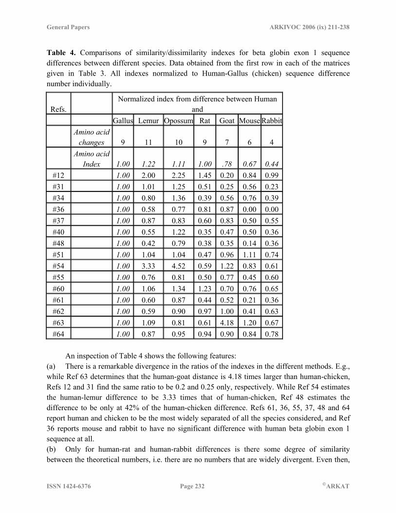
Rat 0 Comparing the differences for the human beta globin exon 1 sequences with the other 7 species in terms of the indexes and the amino acid codes and normalizing to the human-chicken ratio, we obtain the results given in Table 4. Here, reference 61 is based on purely geometrical consideration, while all the other references are based on matrix methods described above.
General Papers ARKIVOC 2006 (ix) 211-238
ISSN 1424-6376 Page 232 ©ARKAT
Table 4. Comparisons of similarity/dissimilarity indexes for beta globin exon 1 sequence differences between different species. Data obtained from the first row in each of the matrices given in Table 3. All indexes normalized to Human-Gallus (chicken) sequence difference number individually.
Refs. Normalized index from difference between Human
and Gallus Lemur Opossum Rat Goat Mouse Rabbit
Amino acid
changes 9 11 10 9 7 6 4
Amino acid
Index 1.00 1.22 1.11 1.00 .78 0.67 0.44 #12 1.00 2.00 2.25 1.45 0.20 0.84 0.99 #31 1.00 1.01 1.25 0.51 0.25 0.56 0.23 #34 1.00 0.80 1.36 0.39 0.56 0.76 0.39 #36 1.00 0.58 0.77 0.81 0.87 0.00 0.00 #37 1.00 0.87 0.83 0.60 0.83 0.50 0.55 #40 1.00 0.55 1.22 0.35 0.47 0.50 0.36 #48 1.00 0.42 0.79 0.38 0.35 0.14 0.36 #51 1.00 1.04 1.04 0.47 0.96 1.11 0.74 #54 1.00 3.33 4.52 0.59 1.22 0.83 0.61 #55 1.00 0.76 0.81 0.50 0.77 0.45 0.60 #60 1.00 1.06 1.34 1.23 0.70 0.76 0.65 #61 1.00 0.60 0.87 0.44 0.52 0.21 0.36 #62 1.00 0.59 0.90 0.97 1.00 0.41 0.63 #63 1.00 1.09 0.81 0.61 4.18 1.20 0.67 #64 1.00 0.87 0.95 0.94 0.90 0.84 0.78
An inspection of Table 4 shows the following features: (a) There is a remarkable divergence in the ratios of the indexes in the different methods. E.g., while Ref 63 determines that the human-goat distance is 4.18 times larger than human-chicken, Refs 12 and 31 find the same ratio to be 0.2 and 0.25 only, respectively. While Ref 54 estimates the human-lemur difference to be 3.33 times that of human-chicken, Ref 48 estimates the difference to be only at 42% of the human-chicken difference. Refs 61, 36, 55, 37, 48 and 64 report human and chicken to be the most widely separated of all the species considered, and Ref 36 reports mouse and rabbit to have no significant difference with human beta globin exon 1 sequence at all. (b) Only for human-rat and human-rabbit differences is there some degree of similarity between the theoretical numbers, i.e. there are no numbers that are widely divergent. Even then,

General Papers ARKIVOC 2006 (ix) 211-238
ISSN 1424-6376 Page 233 ©ARKAT
however, the standard deviations between the numbers reported by the various authors are as large as 50%. In the case of human-goat difference too, leaving out the number 4.18 reported in Ref 63, the standard deviation from the average of the balance figures reported is again 50%. (c) Trend patterns in the ratios for the different species show wide differences between the various methods. Ref 51 shows an almost uniform ratio of around 1 for all species differences with human except for rat where it is 0.47; Ref 48 reports all species to be about 40% as distant from humans as chicken except for human-mouse where it is 0.14 and human-opossum where it is 0.79. Ref 63 swings wildly from 0.61 to 4.18 for the various species whereas Ref 36 has lesser range of variability (0 to 1) but shows a contrary nature to Ref 63 – e.g., while Ref 63 reports the following three ratios compared to the human-chicken difference to be in the order human-lemur > human-opossum > human-rat, Ref 36 reports the same ratios to be in the order human-rat > human-opossum > human-lemur. (d) As compared to the amino acid differences among species, the ratios derived from the DNA sequence descriptors show significant variations. While human-rat differences in the amino acid sequence for the first exon is numerically equivalent to the human-chicken difference, only four of the 15 methods provide a ratio close to this number whereas all others underestimate the differences. The human-mouse difference also shows that only 5 DNA descriptor methods provide ratios reasonably close to the amino-acid difference. We conducted a similar exercise with another set of data based on the same matrices, this time comparing the differences between the sequences of goat with the other species except human. The numbers were normalized to goat-chicken difference. The results again are a mixed bag with wide variations in individual ratios for differences of one species from that of goat. For example, the goat-opossum difference turns out to be 5.9 times higher than the goat-chicken difference in Ref 54 whereas the same ratio is computed to be 0.62 in Ref 36; similarly the goat-rat difference works out to 0.44 times in Ref 36 and 1.45 times in Ref 60 compared to the goat-chicken difference. Trendwise too different methods give results that do not agree: while Ref 62 works out goat-rabbit > goat-lemur > goat-rat, Ref 64 shows the exact opposite result, goat-rabbit < goat-lemur < goat-rat, when compared with the goat-chicken difference. The amino acid differences between goat and the rest of the species turn out to be numerically almost the same, between 23 and 25. None of the papers get the trend or numbers right except Ref 64 which matches with the amino acid difference ratios in the extreme case of rounding to the nearest whole number. 5. Conclusion: the road ahead The basic philosophy of defining mathematical descriptors of DNA sequences is to provide a tool to the biologists in the characterization of sequences in order to derive some kind of relative ranking of the sequences, for mutational or evolutionary studies, or prediction of functional properties. However, when the mathematical descriptors themselves give results contradictory to

General Papers ARKIVOC 2006 (ix) 211-238
ISSN 1424-6376 Page 234 ©ARKAT
one another, and the basic underlying graphical system does not provide any guidance to the problem at hand, the utility of the approach is brought to question. The broad disagreement of the results of the different numerical characterization techniques with the ratios of the amino acid differences can be expected. This is because (a) there is no strict correspondence between the amino acid sequence and the DNA primary sequence because the exon1 does not form strict triplets and also that the exon1 segments of the different species are of different lengths, and (b) none of the methods have really considered the triplet codons to amino acid conversions and their degeneracies in any way. However, theoretical methods need to have contact with reality in some way and with application of the models to exon1 only; there is at this time no other data that can be utilized for comparative analysis and validation of methods. More than that, since each of the methods discussed here applies the particular technique to the same set of sequences, it is to be expected that there will be a broad consensus among the various methods in the relative similarities and dissimilarities among the beta globin exon 1 sequences, irrespective of the absolute numbers computed. The fact that there are very wide discrepancies among the relative indices, as well as broad disagreement among the trends of the indices when comparing different methods, calls into question the relative merits or utility of the various methods that have been proposed so far. At this time, therefore, the way forward would require that authors apply their techniques to complete genes, or at least the complete coding sequence part where the mosaic structures apply, so that an unambiguous point of contact is available for comparing to the real world. Secondly, until a reasonably dependable characterization system is developed, the underlying graphical systems to be used should be the ones with intuitive appeal to understand the base composition and distribution structure in a sequence, and develop numerical techniques based on such graphs. Thirdly, to make mathematical characterization of DNA sequences widely acceptable, the more reliable techniques should be applied to a wide variety of biological problems. With the very rapid rise in DNA sequence data and the strong need for robust quantitative techniques to detect regions of interest in these sequences, mathematical descriptor methods have an important role to play in addressing this need. Lastly, as more quantitative data on the physiochemical as well as biochemical properties of DNA sequences are publicly available, the diverse group of mathematical descriptors discussed here will probably find application in the structure- activity (property) relationships (SAR/SPR) of DNA sequences: This will be analogous to the use of different classes of descriptors, viz., topostructural, topochemical, geometrical, and quantum chemical descriptors, for QSAR of small molecules57. Salient features of a heterogeneous collection of such descriptors or orthogonal variables derived from them may provide a general framework for the quantification of similarity/dissimilarity of DNA sequences65, 66.
General Papers ARKIVOC 2006 (ix) 211-238
ISSN 1424-6376 Page 235 ©ARKAT
Acknowledgements Research reported in this review was supported in part by grant FA9550-05-1-0456 from the United States Air Force. The authors also gratefully acknowledge financial and logistical support from the University of Minnesota and the Natural Resources Research Institute, Duluth, Minnesota. One of us (AN) would like to thank the Consortium for Bioinformatics and Computational Biology, University of Minnesota, Minneapolis for part financial support. This paper is contribution number 424 from the Center for Water and the Environment of the Natural Resources Research Institute. References 1. Johnson, M.; Basak, S. C.; Maggiora, G. Mathl. Comput. Modelling 1988, 11, 630. 2. Basak, S. C.; Niemi, G. J.; Veith, G. D. Journal of Mathematical Chemistry 1991, 7, 243. 3. Basak, S. C.; Niemi, G. J.; Veith, J. Math Chem. 1990, 4, 185. 4. Randic, M.; Witzmann, F.; Vracko, M.; Basak, S. C. J. Med. Chem. Res. 2001, 10, 456. 5. Basak, S. C.; Mills, D. Conference Proceedings 2005, 7, 954. 6. Vracko, M.; Basak, S. C.; Geiss, K.; Witzmann, F. J. Chem. Inf. Model. 2006, 46, 130. 7. Basak, S. C.; Mills, D.; Gute, B. D.; Natarajan, R. In Topics in
Heterocyclic Chemistry Vol. 5: QSAR and Molecular Modeling Studies of Heterocyclic Drugs; Gupta, S. P.; Ed.; Springer-Verlag: Berlin-Heidelberg-New York, in press.
8. Basak, S. C.; Mills, D.; Gute, B. D. In Biological Concepts and Techniques in Toxicology: An IntegratedApproach; Riviere, J. E.; Ed.; Taylor & Francis: New York, NY, 2006; pp 61-82.
9. Roy, A.; Raychaudhury, C.; Nandy, A. J. Biosci. 1998, 23, 55. 10. Berger, J. A.; Mitra, S. K; Carli, M.; Neri, A. J. Franklin Institute 2004, 341, 34. 11. Gates, M. A. J. Theor. Biol. 1986,119, 319. 12. Nandy, A. Current Science 1994, 66, 309. 13. Leong and Morgenthaler, Comput. Appl. Biosci. 1995, 11, 503. 14. Nandy, A. Comput. Appl. Biosci. 1996, 12, 55. 15. Nandy, A. Internet Electron. J. Mol. Des. 2002, 1, 545. 16. Raychaudhury, C.; Nandy, A. J. Chem. Inf. Comput. Sci. 1999, 39, 243. 17. Nandy, A.; Basak, S.C. J. Chem. Inf. Comput. Sci. 2000, 40, 915. 18. Nandy, A.; Nandy, P.; Basak, S. C. Internet Electron. J. Mol. Des. 2002, 1, 367. 19. Wu, Y.; Liew, A. W.; Yan, H.; Yang, M. Chem. Phys. Lett. 2003, 367, 170. 20. Yao, Y.; Nan, X.; Wang, T. J. Mol. Struct. (Theochem) 2006, 764, 101. 21. Ghosh, S.; Roy, A.; Adhya, S.; Nandy, A. Current Science 2003, 84, 1534. 22. Nandy, A.; Nandy, P. Chem. Phys. Lett. 2003, 368, 102.

General Papers ARKIVOC 2006 (ix) 211-238
ISSN 1424-6376 Page 236 ©ARKAT
23. Li, C.;Tang, N.;Wang, J. J.Theo.Biol. in press doi:10.1016/j.jtbi.2005.11.023. 24. Randic, M. J. Chem. Inf. Comput. Sci. 2000, 40, 50. 25. Guo X.; Randic M.; Basak S. C. Chem. Phys. Lett. 2001, 350, 106. 26. Guo, X.; Nandy, A. Chem. Phys. Lett. 2003, 369, 361. 27. Liu, Y.; Guo, X.; Pan, L.; Xu, J.; Wang, S. J. Chem. Inf. Comput. Sci. 2002, 42, 529. 28. Yau, S. S. T.; Wang, J.; Niknejad, A.; Lu, C.; Jin, N.; Ho, Y. Nucleic Acids Res. 2003, 31,
3078. 29. Liao, B. Chem. Phys. Lett. 2005, 401, 196. 30. Liao, B.; Tan, M.; Ding, K. Chem. Phys. Lett. 2005, 414, 296. 31. He, P.; Wang, J. Internet Electron. J. Mol. Des. 2002, 1, 668. 32. Song, J.; Tang, H. J. Biochem. Biophys. Methods 2005, 63, 228. 33. Randic, M.; Vracko, M.; Lers, N.; Plavsic, D. Chem. Phys. Lett. 2003, 368, 1. 34. Randic, M.; Vracko, M.; Lers, N.; Plavsic, D. Chem. Phys. Lett. 2003, 371, 202. 35. Yao, Y.; Liao, B.; Wang, T. J. Mol. Struct. (Theochem) 2005, 755, 131. 36. Li, C.; Wang, J. Combinatorial Chem. & High Throughput Screening 2003, 6, 795. 37. Liao, B.; Wang, T. J. Comput. Chem. 2004, 25, 1364. 38. Liao, B.; Ding, K. J. Comput. Chem. 2005, 26, 1519, 1523. 39. Wang, J.; Zhang, Y. Chem. Phys. Lett. 2006, 423, 50. 40. Yao, Y.; Wang, T. Chem. Phys. Lett. 2004, 398, 318. 41. Randic, M.; Vracko, M.; Zupan, J.; Novic, M. Chem. Phys. Lett. 2003, 373, 558. 42. Randic, M. Chem. Phys. Lett. 2004, 386, 468. 43. Randic, M.; Zupan, J. SAR and QSAR Environ. Res. 2004, 15, 191. 44. Jeffrey, H. J., Nucleic Acids Res. 1990, 18, 2163. 45. Hamori, E.; Ruskin, J. J.Biol.Chem. 1983, 258, 1318. 46. Randic, M.; Vracko, M.; Nandy, A.; Basak, S. C. J. Chem. Inf. Comput. Sci. 2000, 40, 1235. 47. Li, C.; Wang, J. Combinatorial Chemistry & High Throughput Screening 2004, 7, 23. 48. Yao, Y.; Nan, X.; Wang, T. Chem. Phys. Lett. 2005, 411, 248. 49. Yuan, C.; Liao, B.; Wang, T. Chem. Phys. Lett. 2003, 379, 412. 50. Liao, B.; Wang, T. J. Mol. Struct. (Theochem) 2004, 681, 209. 51. Liao, B.; Zhang, Y.; Ding, K.; Wang, T. J. Mol. Struct. 2005, 717, 199. 52. Zhu, W.; Liao, B.; Ding, K. J. Mol. Struct. 2005, 757, 193. 53. Bai, F.; Zhu, W.; Wang, T. Chem. Phys. Lett. 2005, 408, 258. 54. Chi, R.; Ding, K. Chem. Phys. Lett. 2005, 407, 63. 55. Liao, B.; Wang, T. J. Chem. Inf. Comput. Sci. 2004, 44, 1666. 56. Randic, M.; Lers, N.; Plavsic, D.; Basak, S. C.; Balaban, A. T. Chem. Phys. Lett. 2005, 407,
205. 57. Devillers, J.; Balaban, A., Eds.; Topological Indices and Related Descriptors in QSAR and
QSPR; Gordon and Breach Science Publishers: The Netherlands, 1999, pp 675-696. 58. Basak, S. C.; Mills, D.; Gute, B. D. In Advances in Quantum Chemistry, Klein, D. J.,
Brandas, E., Eds.; Elsevier, in press.
General Papers ARKIVOC 2006 (ix) 211-238
ISSN 1424-6376 Page 237 ©ARKAT
59. Randic, M.; Witzmann, F.; Vracko, M.; Basak, S. C. Med. Chem. Res. 2001, 10, 456. 60. He, P.; Wang, J. J. Chem. Inf. Comput. Sci. 2002, 42, 1080. 61. Randic, M.; Vracko, M. J. Chem. Inf. Comput. Sci. 2000, 40, 599. 62. Randic, M.; Guo, X.; Basak, S. C. J. Chem. Inf. Comput. Sci. 2001, 41, 619. 63. Randic, M.; Balaban, J. Chem. Inf. Comput. Sci. 2003, 43, 532. 64. Ying-zhao; Wang, T. Chem. Phys. Lett. 2006, 417, 173. 65. Basak, S. C.; Magnuson V. R.; Niemi, G. J.; Regal, R. R. Discrete Appl. Math 1988, 19, 17. 66. Basak, S. C.; Mills, D.; Gute, B. Arkivoc 2006, (ix), 157. Authors’ biographical data
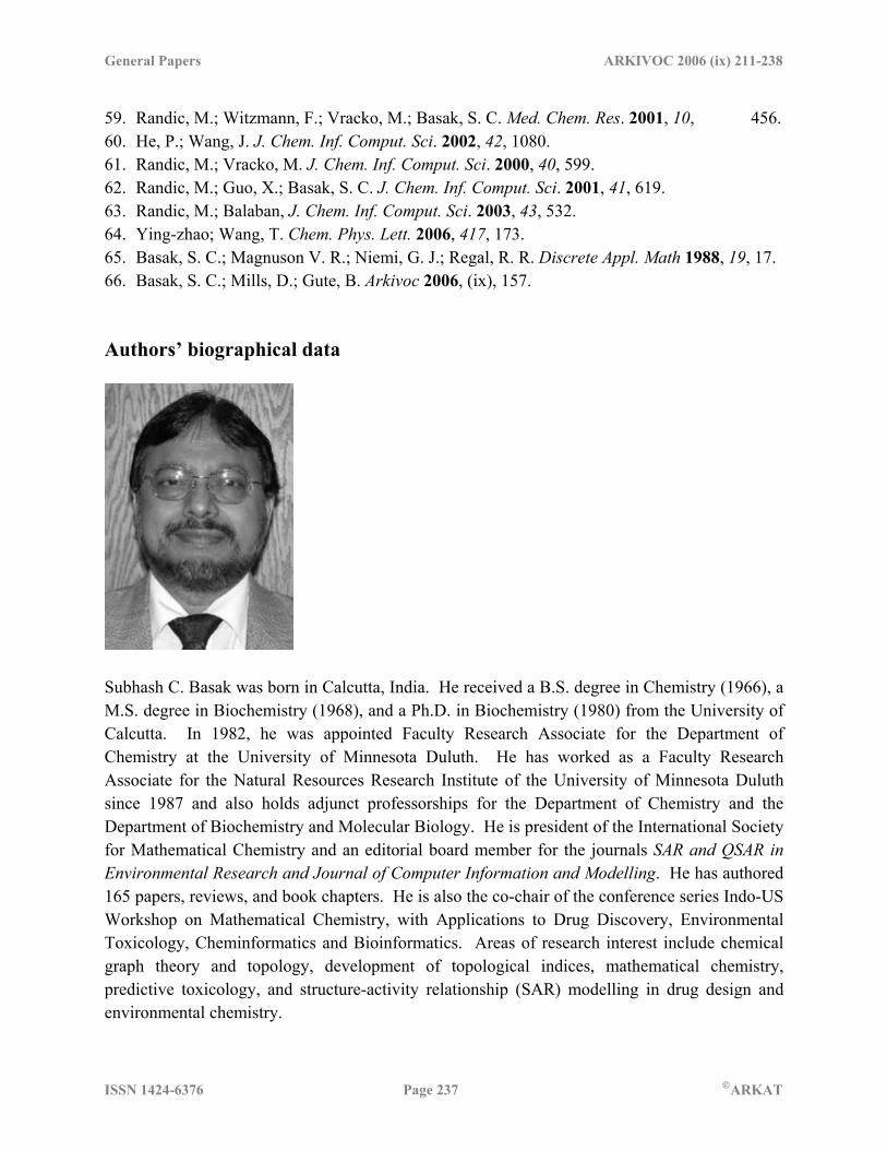
Subhash C. Basak was born in Calcutta, India. He received a B.S. degree in Chemistry (1966), a M.S. degree in Biochemistry (1968), and a Ph.D. in Biochemistry (1980) from the University of Calcutta. In 1982, he was appointed Faculty Research Associate for the Department of Chemistry at the University of Minnesota Duluth. He has worked as a Faculty Research Associate for the Natural Resources Research Institute of the University of Minnesota Duluth since 1987 and also holds adjunct professorships for the Department of Chemistry and the Department of Biochemistry and Molecular Biology. He is president of the International Society for Mathematical Chemistry and an editorial board member for the journals SAR and QSAR in Environmental Research and Journal of Computer Information and Modelling. He has authored 165 papers, reviews, and book chapters. He is also the co-chair of the conference series Indo-US Workshop on Mathematical Chemistry, with Applications to Drug Discovery, Environmental Toxicology, Cheminformatics and Bioinformatics. Areas of research interest include chemical graph theory and topology, development of topological indices, mathematical chemistry, predictive toxicology, and structure-activity relationship (SAR) modelling in drug design and environmental chemistry.

General Papers ARKIVOC 2006 (ix) 211-238
ISSN 1424-6376 Page 238 ©ARKAT
Marissa Harle is a graduate student in the Department of Chemistry at the University of Minnesota in Duluth. She is interested in doing research in Bioinformatics.
Ashesh Nandy did his PhD in theoretical physics and later switched to computational biology. His interest is in modelling and analysis of DNA sequences.


![Mathematical properties of DNA sequences from coding and ...periodicities in coding and noncoding regions [3]. They stud-ied sequences from virus, prokaryotes, and eukaryotes, and](https://static.fdocuments.in/doc/165x107/60f82fab10bcaa70227608b5/mathematical-properties-of-dna-sequences-from-coding-and-periodicities-in-coding.jpg)