preprint

Mathematical characterization of the transduction chain in growth cone

pathfinding

Giacomo Aletti · Paola Causin

Abstract Axon guidance by graded diffusible ligands plays an important role in the developing nervous

system. Concentration gradients induce an asymmetric localization of molecules in the axon tip, the growth

cone, and the consequent internal polarized signaling pathway leads to rearrangement of the growth cone

cytoskeleton and, ultimately, to motility. In this work, we provide a mathematical description of the growth

cone transduction chain as a series of functional boxes characterized by input/output relations. The model

relies on the assumption that the characteristic time of independent concentration measures by growth

cone receptors, the characteristic time of growth cone internal reorganization preceding motion and the

characteristic time needed for a discernible axon turning belong to separated scales. The results give

insight into the deterministic vs. stochastic regime of internal growth cone functions that are not readily

accessible from experimental observations, pointing out a substantial equilibrium of the two contributions.

The mathematical model predicts the decrease of the coefficient of variation of the signal moving down the

functional chain leading to motion. Moreover, possible mechanisms that allow for buffering against noise

are highlighted. These results have an interest also for the more experimentally-minded reader, since they

can be used to predict sample sizes for detecting significant differences in benchmark gradient assays.

Keywords Growth cone pathfinding · Chemotaxis · Mathematical model · Computational model ·Ornstein-Uhlenbeck process

Mathematics Subject Classification (2000) 92B05 · 60G35 · 65N30

1 Introduction

In the developing embryo, neurons form connections by projecting axons to appropriate target areas.

Pathfinding crucially relies on extracellular cues present in the environment [37]. Axons can be guided

by diffusible chemoattractant substances secreted at some distance by intermediate or final targets [38];

long-range chemorepulsion exists as well, demonstrated by the fact that axons can be repelled by dif-

fusible factors [8]. Contact-mediated mechanisms involving interaction with substrate bound nondiffusible

molecules are also known to play an important role, both in terms of contact attraction [23] or contact

inhibition [25].

G. Aletti, P. CausinDipartimento di Matematica “F. Enriques”, Universita degli Studi di Milano, via Saldini 50, 20133 Milano, Italy.E-mail: aletti,causin@mat.unimi.it

2

In this paper, we focus on guidance by gradients of diffusible chemoattractant ligands; this process has

been described for different molecules, including netrins, semaphorins, neurotransmitters (see, e.g., [37,30,

33]). The growth cone (GC), located at the axon tip, is a highly motile structure that mediates detection

and transduction of navigational cues [15,13]. Chemotropic gradients across the GC diameter are often

quite small. Studies of cultured Xenopus spinal neurons showed that the GC can respond to a gradient of

diffusible attractants of about 5 − 10% across its diameter [44,33]. In the theoretical analysis of [10], the

minimum percentage change of concentration detectable by a GC is indicated in 1−2%. In [32], a gradient

percentage change as low as 0.1% is used to induce axon turning. Despite these shallow gradients, a steeper

internal polarization arises in the GC [5], which leads, in turn, to a rearrangement of the GC cytoskeleton

and, ultimately, to motility [19,24].

During the last decade, several studies have focused on deciphering portions of the signaling pathway

and identifying the role of various molecules (see, e.g., [33,15,41]). The understanding of the complete

organization of the GC transduction machinery is a highly complex task still far from being completed,

so that phenomenological mathematical models can play a significant role in assessing the main physical

properties of the underlying intracellular transformations [11,28]. The benchmark chemotaxis assay studies

the response of GCs exposed to steady graded concentrations of a single attractive/repulsive ligand [44,

45,29]. Turning angles and standard error parameters are measured after a certain time interval from the

onset of the gradient. Data are tabulated as a function of ligand concentration and (less often) of gradient

percentage change (steepness). Different mathematical and computational models have been developed to

account for these results. The computational model of [6] focuses on two distinct modes of GC motility.

The first mode characterizes motility on homogeneous substrates and is based on a Langevin equation

(persistent random walk model) where the velocity decreases as an exponential function of time, with

sudden increases/variations in the speed due to random “kicks” arising from Gaussian noise terms. A

second mode characterizes motility on patterned substrates in which the GC appears to move in a biased

fashion along preferential paths. The concept of resistance of GC to directional changes is advanced and

modeled as a “residence time” of stationarity of order comparable to a characteristic time (the value 360s

is used in simulations) between deviations in the trajectory. In the seminal work [4], physical constraints

underlying concentration measures by a small sensing device with a limited number of receptors are ana-

lyzed. Predictions of the statistical fluctuations arising from the estimation of the concentration and of the

time needed to carry out independent measurements are formulated. Based on this theoretical analysis,

in [12] the minimum detectable gradient steepness, the maximum range of guidance, and the sensitiv-

ity as a function of ligand concentration are discussed in the case of GCs and compared to experiments

(see also [10]). A further computational model is investigated in [11], where filopodia, thin filaments that

protrude from the GC surface, act as antennae-like devices to guide the GC. Guidance is mediated by

ligand receptors located on filopodia and on the GC surface: the gradient of receptor binding across the

GC diameter is supposed to produce a difference in the likelihood of generating new filopodia. Filopodia

production is enhanced/inhibited in the angular sector facing the attractant/repellent source. This effect

represents a positive feedback mechanism. The new orientation of the GC is a combination of the previous

orientation plus a function of the average angle of receptor binding. Inertial (memory) effects are kept into

account by weighting the two contributions for the 97% and the remaining 3%, respectively. In [42], the

same authors consider a conceptually similar model, adding spatial and temporal averaging of stochastic

receptor–binding signal in order to obtain a close fitting with experimental GC sensitivity. A timescale of

about 100 − 200s of averaging (characteristic time of signal decay) is found to be adequate, considering

that a time interval of the order of 10s is needed to obtain an independent measurement of concentration.

In [1], a step towards the introduction of internal dynamics is done, by relating the angular distribution

of filopodia to the angular variation of ionic calcium diffused in the periphery of the GC. In [27,28], a

simple model of random walk is adopted to describe GC migration in response to a contact cue. In order

to quantify the deterministic and stochastic components of such a motion, a dimensionless number Ψ is

introduced, representing the ratio between the sum of the mean deterministic migration over the stochas-

3

tic migration in a characteristic time. Only when Ψ is of the order of the unity, constructive guidance is

shown to be possible, this value corresponding to a characteristic time of 10 − 90s, comparable to the GC

reorganization time in response to a stimulus. In [17,18], the formation of a coherent axonal organization

is investigated under the hypothesis that guidance is driven by steady–state diffusible chemoattractants

and chemorepellants as well as by contact attraction/repulsion. In [22], finite–dimensional state vectors

in an ordinary differential equation system describe the deterministic macroscopic motion of the GC and

the dynamical evolution of its internal state, respectively. Reviews of mathematical models for studying

different phases of neurite outgrowth (initiation, elongation, branching) can be found in [20,14].

In this work, we model the GC transduction chain as a series of functional tasks, which lead from

gradient sensing to signal transduction, down to motion actuation. The mathematical representation maps

input/output signals of each unit, without reproducing intracellular chemical processes. Such modeling

is based on the identification of three characteristic times –corresponding to independent concentration

measure by GC receptors, GC internal reorganization preceding motion and discernible axon turning–

which belong to separated scales, ranging from the smaller to the larger ones. The key elements of di-

rectional response towards a target, memory effect and randomness are translated into the mathematical

form of an Ornstein–Uhlenbeck process, which models the central transduction box. Insights into the de-

terministic vs. stochastic regime of internal GC functions that are not readily accessible from experimental

observations are gained through descriptive statistical indexes of output signals. Referring in particular

to the test setting of the gradient chemotaxis assay, the model predicts the decrease of the coefficient of

variation of the output signal moving down the functional boxes of the chain. The transduction process

is shown to be in equilibrium between deterministic and stochastic regimes. A mechanism that allows for

buffering against noise is highlighted in the motor actuator function, in which inertia exerts a smoothening

effect that contributes to produce the relatively straight paths of GCs (like the ones observed on in vitro

experiments [33]). An analysis of the origin of the stochastic contribution is carried out, predicting the

transduction process to be a main source of noise. The mathematical model presented in this work has

a point of interest also for the more experimentally-minded readers. Some literature papers on in vitro

gradient assays present results on axon turning angles (see the discussion of Sect. 3) displaying a tendence

toward biased trajectories, without being statistically significant. Our results show that the sample sizes

needed for detecting statistical significant difference of axonal response are bigger compared to the sample

size commonly used in experiments. Moreover, when carrying out assays with a single steady–state cue,

our model shows how a single pilot test, precursor to a full-scale study, may be used to evaluate sample

sizes for different analyses.

The remaining of the paper is organized as follows. In Sect. 2 we present the mathematical model,

yielding the stochastic differential law for the GC trajectory. In Sect. 3 we introduce the descriptive

statistical indexes that characterize the transduction process. In Sect. 4 the results of the above sections

are discussed. Finally, in Sect. 5 the conclusions are drawn, reviewing the validity of the proposed model.

2 Model description

We consider a synthetic representation of the transduction chain of the GC, which leads from sensing of

ligand concentration gradients to motion. Measures of concentration differences ∆C in the environment

are produced by the Sensing Device Box (SDBox). The Signal Transduction Box (STBox) processes the

input from the SDBox performing an appropriate amplification of the signal (see, e.g., [11] for a mathe-

matical model of amplification functions). Actin reorganization in the GC cytoskeleton, directly preceding

motion [34,35], is activated by the STBox signal (see [43,33,24] for discussions on activated signal path-

ways). The Motor Actuator Box (MABox) produces a deviation of the trajectory. Fig. 1 (top row) depicts

the successive steps of the chain, together with their characteristic times. The gradient sensing process

takes place in a time of the order of tenths of seconds, signal transduction and internal reorganization

4

Parameter Meaning

∆C Ligand concentration difference across the GC diameterbP Mean asymptotic value of the equivalent forcePt = (Xt, Yt) Actual value of the equivalent forceP

∗t Dimensionless equivalent force

m equivalent massλ Memory effect parameterτ, θ Time persistence parametersσ Volatility parametervg GC velocity vector (vg velocity modulus, eg velocity direction)α Angle between the GC direction and the x-axisβ Angle between the GC direction and the equivalent forceγ Measure of turning angle in benchmark experimentsCV Coefficient of variationAI Accuracy indexk Accuracy index ratioN Sample sizeα, 1 − β Type I error and power in statistical testsS.E.M Standard Error of the Mean

Table 1 Model parameters and their meaning. For parameter values used to derive numerical results, see text.

in a time of the order of a few minutes, trajectory deviations in a time of the order of tenth of minutes.

Fig. 1 (bottom row) gives a representation of the mathematical model corresponding to each biological

phenomenon. Parameters and their meaning are given in Table 1.

concentration

field PtSensing

Device

Signal

TransductionMotor

Actuator

α(t)bP∆C

10s 200s 10m

Fig. 1 Top row: cascade of macroscopical phenomena leading from gradient sensing to motion. Receptor bindingstate produces data on the concentration field; the polarized signaling pathway enhances reorganization of internalGC cytoskeleton; the trajectory is deviated. Characteristic times are indicated for each process. Bottom row: signalprocessing chain in the mathematical model. Sensing Device, Signal Transduction and Motor Actuator functions.Inputs and outputs refer to quantities of system (7).

2.1 Mathematical model of the SDBox

Receptors located on the GC surface and filopodia bind to external ligands. The density function of bound

receptors around the GC can be used to model the process of ligand concentration sensing, as proposed

for example in [1,11]. In the present model, we do not consider such a physical process, but we directly

model the output of the SDBox as a mathematical object, the vector bP which triggers the deviation of the

GC trajectory (Fig. 1, leftmost panel of bottom row). This idea stems from the fact that a concentration

5

gradient orients the GC motion toward the direction of the concentration source. According to a mechanical

description, we ascribe the trajectory deviation to an equivalent force vector process Pt acting on an

equivalent GC mass m. The process Pt, output of the STBox (see the next section for a detailed study),

is continuously attracted towards bP . The vector bP is a function of ∆C: its direction is related to the

orientation of the stimulus gradient, while its modulus is connected to the amplification produced by the

GC transduction chain. We observe that a conceptually similar approach is used in [42], where the GC

responds to the stimulus along a direction connected to the mean value of the angle of maximum receptor

binding (the quantity φmax) and with a modulus given by the sensitivity surface function of [42, Fig.4].

2.2 Mathematical description of the STBox

The role of the STBox is to compare the output bP of the SDBox, function of the external signals, against

an “equivalent” actual force Pt (Fig. 1, central panel of bottom row). In this process, a memory effect exists

(see also [42, Sect. Mathematical models]), which damps the response, so that the updated equivalent force

is written as

Pt+δt = (1 − λ)Pt + λ eP , (1)

where λ ∈ [0, 1] is a weighting factor and eP is the contribution arising from the comparison. If the

time interval δt is long enough, eP can be assumed statistically independent from Pt and written as

eP = bP + σq

2λZ. where Z denotes a two–dimensional standardized random vector independent of Pt,

σ = σ( bP ) is a volatility parameter and the factorp

2/λ appears due to a normalization choice. One may

also think that the comparison produces an incremental “kick” δP [6], yielding Pt+δt = Pt + δP . From

Eq. (1), we obtain that the kick is composed of a deterministic part, representing its mean effect E(δP )

which re–orients the response towards bP and of a random part. The first term acts as a linear spring of

constant λ: E(δP ) = −λ(Pt − bP ), while the second term is a distribution independent of Pt (but possibly

depending on bP ). Let λ =δt

τ, τ being a persistence time. Then, δP can be written as

δP = −Pt − bPτ

δt| {z }E(δP )

+ σ√

δt

r2

τZ

| {z }δP−E(δP )

. (2)

If we consider time scales larger than δt, Eq. (2) tends to the continuous generalized Ornstein–Uhlenbeck

(OU) process, which is assumed to obey to Ito calculus (see for example [3])

dPt = −Pt − bPτ

dt + σ

r2

τdWt, (3)

where Wt denotes a two–dimensional Wiener process. When bP does not depend on time, σ is constant

and the solution of (3) reads

Pt = bP + (P0 − bP )e−t/τ +

Z t

0σ

r2

τe(s−t)/τ dWs. (4)

Relation (4) shows that the mean value of Pt tends exponentially fast in time to bP . Moreover, Ito’s

lemma [3] implies that at steady–state, Pt is a bivariate Gaussian distribution with subjected to an isotropic

random perturbation of bounded variance σ2. Moreover, the autocorrelation function for each component

of the process Pt is

R(s) = limt→+∞

R(t, t + s) = e−s/τ , (5)

which implies that the time after which practically independent outputs are produced is proportional to τ .

6

f

eg

GC

α

e⊥

attractive cue

β

x

Pty

Fig. 2 Notation for the mathematical model of GC motion.

2.3 Mathematical description of the MABox

We suppose that the equivalent force Pt induces an acceleration only along the direction transversal to

the trajectory (see also [22] for a similar hypothesis). Consequently, if the axon moves with velocity vector

vg = vgeg (vg = 20−30µm/h, [39]), only the direction of the unit vector eg is affected, leaving the velocity

modulus constant. The following equation of dynamical equilibrium describe the transversal motion of the

GC (see Fig. 2 for notation)

ma = |Pt| sin β, (6)

where a is the transversal acceleration, m is the GC equivalent mass, β is the angle between eg and Pt

and we have supposed a negligible internal mechanical reaction in the axon shaft along the transversal

direction. The acceleration changes the angle α that eg forms with the horizontal direction. Notice that

when Pt is such that E(Pt) = 0, the trajectory is not deterministically deviated. This models the physical

fact that, in absence of ligand gradients and at least on in vitro experiments, axons tend to follow noised

trajectories with no significant bias from their initial growth direction [9].

2.4 Mathematical model of the GC trajectory law

Based on the above considerations, the complete model of the GC motion reads:

given bP ,1 find for 0 ≤ t ≤ T the GC position xg = xg(t), such that

xg = vg,

vg =|Pt| sin β

me⊥,

dPt = −Pt − bPτ

dt + σ

r2

τdWt,

xg(0) = x0g,

vg(0) = vge0g,

P0 = P0,

(7)

1 Notice that bP , being a function of ∆C, may actually depend on time and on the spatial position.

7

where x0g, v

0g are the given initial position and direction of the axon GC. Eq. (7)3 models the STBox

input/output relation, while Eq. (7)1,2 model the MABox input/output relation. System (7) is a stochastic

differential system and can be numerically solved by using a stochastic Runge–Kutta integration scheme

(see for example [21]).

In order to determine the asymptotic equivalent acceleration bP /m, we consider experimental data from

the benchmark gradient assay [44,29,32]. The mean velocity variation during a time interval ∆t due to bPE[∆vg] =| bP |∆t

msin(β)e⊥,

leads to a mean angle variation of the trajectoryE[∆α] =| bP |mvg

sin(β)∆t, (8)

to which we can associate the curvature radius

Rc =vg∆tE[∆α]

=vg

| bP |mvg

sin(β). (9)

The minimum of Rc

Rc,min =mv2

g

| bP |, (10)

occurs when the trajectory of the axon is orthogonal to the ligand gradient (sin β = 1). From the experi-

mental quantities vg and Rc,min, we can thus estimate

| bP |m

=v2g

Rc,min. (11)

Remark 1 Notice that using (10) into Eq. (8), we getE[∆α] =vg

Rc,minsin(β)∆t,

which recovers the deterministic macroscopic GC model of [22, Eq. (28)].

3 Descriptive statistical indexes of the transduction chain

The variability of the stimulus–response maps of each functional box can be characterized by the variance

and the coefficient of variation of the box output. In particular, the coefficient of variation, defined as

the ratio between the standard deviation and the expected value of a distribution, is a dispersion index

that relates the weight of the stochastic and deterministic effects. We use this parameter to assess the

importance of the stochastic component over the deterministic one in the outputs of the functional chain.

8

0 0.5 1 1.5−0.4

−0.2

0

0.2

0.4

0.6

CVP ≪ 1

−10 −5 0 5 10−10

−5

0

5

10

CVP ≈ 1

−400 −200 0 200−400

−200

0

200

400

CVP ≫ 1

−20 0 20 40

−10

0

10

20

30

40

−20 0 20 40

−10

0

10

20

30

40

−20 0 20

−10

0

10

20

30

40

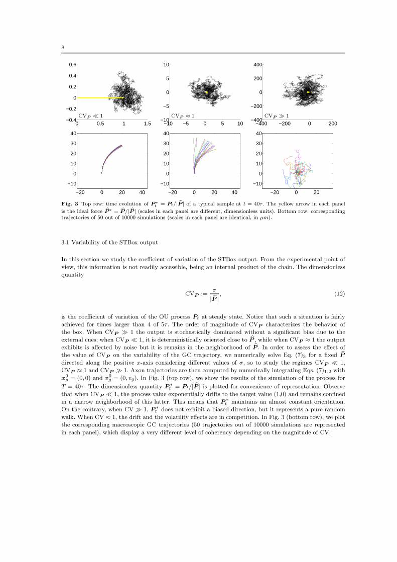
Fig. 3 Top row: time evolution of P∗t = Pt/| bP | of a typical sample at t = 40τ . The yellow arrow in each panel

is the ideal force bP∗ = bP/| bP | (scales in each panel are different, dimensionless units). Bottom row: correspondingtrajectories of 50 out of 10000 simulations (scales in each panel are identical, in µm).

3.1 Variability of the STBox output

In this section we study the coefficient of variation of the STBox output. From the experimental point of

view, this information is not readily accessible, being an internal product of the chain. The dimensionless

quantity

CVP :=σ

| bP |, (12)

is the coefficient of variation of the OU process Pt at steady state. Notice that such a situation is fairly

achieved for times larger than 4 of 5τ . The order of magnitude of CVP characterizes the behavior of

the box. When CVP ≫ 1 the output is stochastically dominated without a significant bias due to the

external cues; when CVP ≪ 1, it is deterministically oriented close to bP , while when CVP ≈ 1 the output

exhibits is affected by noise but it is remains in the neighborhood of bP . In order to assess the effect of

the value of CVP on the variability of the GC trajectory, we numerically solve Eq. (7)3 for a fixed bPdirected along the positive x-axis considering different values of σ, so to study the regimes CVP ≪ 1,

CVP ≈ 1 and CVP ≫ 1. Axon trajectories are then computed by numerically integrating Eqs. (7)1,2 with

x0g = (0, 0) and v

0g = (0, vg). In Fig. 3 (top row), we show the results of the simulation of the process for

T = 40τ . The dimensionless quantity P∗t = Pt/| bP | is plotted for convenience of representation. Observe

that when CVP ≪ 1, the process value exponentially drifts to the target value (1,0) and remains confined

in a narrow neighborhood of this latter. This means that P∗t maintains an almost constant orientation.

On the contrary, when CV ≫ 1, P∗t does not exhibit a biased direction, but it represents a pure random

walk. When CV ≈ 1, the drift and the volatility effects are in competition. In Fig. 3 (bottom row), we plot

the corresponding macroscopic GC trajectories (50 trajectories out of 10000 simulations are represented

in each panel), which display a very different level of coherency depending on the magnitude of CV.

9

α

vg

Xt

Yt

x

y

α

π2− α

vg

γ

O′O

P

Fig. 4 Left: notation for the benchmark gradient assay and Eq. (13). Right: Approximation for small values of γ.Notice that, with respect to the circumference of center O′ passing through O and P , γ = (π/2 − α)/2, since it isthe inscribed angle corresponding to half the central angle π/2 − α.

3.2 Variability of the MABox output

In order to study the variability of the MABox, we consider the standard gradient assay. A single steady

gradient of a chemoattractant ligand is established along the positive x-axis. Axons initially grow along

the direction of the positive y-axis, starting from the origin. We study the variance and the coefficient of

variation of the axon turning angle γ, defined as the angle between the y axis and the line connecting the

origin and the position of the GC at a certain time after the onset of the gradient application (see Fig. 4,

left and refer to [44,45,32] for experimental results).

Throughout the section, we consider Eq. (7)2 written in terms of the angular coordinate α, which is

connected to the linear velocity vg by vg = vge⊥α. Eqs. (7)2−3 becomes

α = − Xt

mvgsin α +

Yt

mvgcos α,

dXt = −Xt − | bP |τ

dt + σ

r2

τdW 1

t ,

dYt = −Yt

τdt + σ

r2

τdW 2

t ,

(13)

where we have introduced the (x, y) components (Xt, Yt) of Pt (see Fig. 4, left), and W 1t and W 2

t are

independent Brownian processes. For small variations of α, it is possible to consider a simplified version of

system (13), on which it is more straightforward to compute the statistical indexes. Under this hypothesis,

we have that γ ≃ (π/2 − α)/2 (see Fig. 4, right) and system (13) can be written as

γ =Xt

2mvg,

dXt = −Xt − | bP |τ

dt + σ

r2

τdW 1

t .

(14)

The turning angle (14) is thus an integrated OU process. On in vitro experiments, the steady–state distri-

bution of Xt is reached in a relatively short time. In these conditions, one may assume that E(Xt) = | bP |

10

for all times. With this hypothesis, and recalling that for the OU process Xt the covariance reads

Cov(Xs, Xv) = σ2 e−v+s

τ (e2 min(s,v)

τ − 1),

we compute from (14)

Var(γ) =1

4m2v2gVar

“ Z t

0Xs ds

”

=1

4m2v2gE„“ Z t

0(Xs − | bP |) ds

”2«

=1

4m2v2g

Z t

0

Z t

0Cov(Xs, Xv) ds dv

=1

4m2v2g

σ2τ`2t − 3τ + 4τe−

tτ − τe−2 t

τ´.

Its first order approximation reads

Var(γ) ≃ σ2t τ

2m2v2g

. (15)

Then, we have

std(γ(t)) =`Var(γ)

´1/2 ≃ σ√

τ t√2mvg

. (16)

and we compute the coefficient of variation of γ

CVγ(t) =std(γ(t))E(γ(t))

≃ σ

| bP |

r2τ

t. (17)

In order to assess the results of this section, we solve the complete system (13) (equivalent to (7))

simulating 5000 axons trajectories, each starting from the origin and initially directed along the positive

y–axis. For each simulation we consider a total time of 2h, τ = 200s and we use a time step of 10s.

Fig. 5(left) shows std(γ(t)) as a function of σ. Fig. 5(right) shows E(γ(t)) and std(γ(t)) as a function of

time. In the same figures we plot in dotted lines the approximate analytical expressions (16) and (17).

Notice that, despite the simplifications, the the results of the complete numerical integration of are well

reproduced, so that (16) and (17) provide a good prediction of the effective behavior.

3.3 Accuracy of the MABox

The MABox acts as a filter processing a noised input signal to obtain another signal. In order to evaluate

the performance of this function, we introduce the accuracy index AI, defined as the reciprocal of the

coefficient of variation, AI := 1/CV. We consider the following “accuracy index ratio” k

k :=AIγ(t)

AIPt

≃r

t

2τ, (18)

where we have used the approximate results of the previous section. The index k represents the amplification

of the accuracy of the signal. It grows monotonically with time, coherent with the fact that a significantly

biased motion is observed only after a time long enough, of the order of some multiples of τ .

Analogously to what done in the previous section, we solve the complete system (13) simulating 5000

axons trajectories and for each we compute the accuracy indexes AIPt, AIγ(t) and the accuracy index

11

std(γ

(t))

σ

0.160.30.50.831.52

0 0.5 1 1.5 20

5

10

15

20

25

E(γ(t))std(γ(t))

t

Fig. 5 Left: numerical integration of (7) shows the linear dependence of σ and std(γ(t)). Each curve is parametrizedfor different time values (in hours). Right: the expected value of γ and its variance vary linearly with time and asthe square root of time, respectively (angles are in degrees, time in hours).

ratio k. In Fig. 6(left) the coefficient AIγ(t) is plotted as a function of AIPtfor different times. Fig. 6(right)

shows the factor k as a function of time. Fig. 6(bottom) shows AIγ againstq

t2τ AIPt

. Approximate

analytical results are reported on the figures in dotted lines. Again, despite the simplifications, theoretical

predictions are in good agreement with the full model results.

4 Discussion

4.1 Choice of the mathematical model

GCs subjected to a graded field of an attractive ligand describe noised paths in the direction of the

concentration source. This behavior can be mathematically modeled by an OU process. In Eq. (13), the

OU process is a model for the angular velocity α (or for the linear acceleration); one may wonder whether

the OU process should rather model the evolution of the angular variable α. This latter model should read

dαt = −αt − bαθ

dt + σαdWt, (19)

where bα is the asymptotic mean response to the given gradient, θ is a time persistence parameter and σα

is a volatility parameter. A SDE equation of the type (13) or (19) produces solutions that are continuous

but non differentiable. Thus, in model (13) (resp. (19)) the angular velocity (resp. angular variation) is

a continuous function with no time derivates: a white noise process is observed in α (resp. α). Changes

in the external solicitations require a certain reorganization time before being effective [45]. This suggests

that the velocity of adaptation should be at least a bounded continuous function of time, which leads to

model (13). Further elements of discrimination for the model choice are much more critical. If smoothness of

the trajectories is taken as a decision parameter, even if model (19) produces C1 paths, while model (13)

produces more regular C2 paths, experimental data do not provide a quantitative evidence for such a

discrimination (see also the discussion of [28, Integrated Random Walks]). A further observation stems

from the meaning of characteristic times: τ represents the time of reorganization of the GC (∼ 200s), while

θ in Eq. (19) represents the time of a significant change of the mean angle (several minutes). As such,

τ ≪ θ and the computation of the respective Var(γ(t)) and CVγ adopts asymptotic vs. infinitesimal time

12

0 0.5 1 1.5 2 2.5 3 3.50

2

4

6

8

10

12

14

0.96

1.4

1.76

2.34

3.23

3.86

AIPt

AI γ

(t)

0.160.30.5

0.831.52

0 0.5 1 1.5 20

0.5

1

1.5

2

2.5

3

3.5

t

k

qt

2τ

0 2 4 6 8 10 120

2

4

6

8

10

12

AIPt

rt

2τ

AI γ

(t)

Fig. 6 Top left: dependence of the accuracy index of the MABox output with respect to the accuracy index ofthe MABox input. Curves are parametrized in time (hours) specified in the legend, numerical values on the curves

represent the amplification k. Top right: the amplification k mimics the functionp

t/(2τ) as predicted by Eq. (18)(time is in hours). Colors are the same as in the top left panel, data in black are additional values. Bottom:

approximation AIγ(t) ≃q

t2τ

AIPt. The dashed line is the theoretical linear dependence. Colors are the same as in

the top left panel, data in black are additional values.

expansions. In any case, both the model of Eq. (13) and the alternative model of Eq. (19) show the same

dependence of statistical indexes with respect to time (std(γ(t)) ≍ t1/2, CVγ ≍ t−1/2), and again these

quantities –that can be connected to experimental results– do not represent an useful discriminant test.

4.2 Stochastic vs. deterministic regime of the STBox output

Experimental data may be used to characterize the regime of variability of the STBox output, which is a

hidden information from the macroscopic point of view. Referring to the benchmark gradient assay data

13

of [44], we compute

CVγ =std(γ(t))E(γ(t))

≃ S.E.M.√

N

γ≃ 1.16 ,

where S.E.M. is the standard error of the mean of γ(t), N is the number of cells examined, γ is the

average of the measured values of the turning angles and the experiments are carried out for a time t = 2h.

Comparable values are obtained from similar experiments, see e.g., [29,32]. From Eq. (18), using τ = 200s,

we estimate CVP ≃ 5, which, being of the order of the unity, shows that stochastic and deterministic effects

act with comparable magnitude. This mechanism represents a “robust” process with respect to fluctuations:

axons effectively reach their target following a graded concentration field (expression of organization) while

allowing for a large amount of noise (expression of variability). This is an energetic trade–off: the STBox

output is the most noised signal that can be accepted without losing the underlying directional message

(see also [27,28]).

The coefficient of variation provides information on the amplitude of the signal deviations from the

average. Information about the time frequency of such deviations are contained in the characteristic times.

When modeling the GC function of sensing with a characteristic time of the order of δt, the introduction of

a memory effect as in Eq. (1), dilates the non–correlation time of the signal from δt to τ (see Eq. (5)). The

ratio λ of the two times is the factor of dilation. As λ decreases, the system dumps out high frequencies,

avoiding sharp variations in the output Pt.

4.3 Origin of stochastic noise

Experimental data collected for different concentration fields [44,29,32] mean values of the turning angle

with a substantially constant Var(γ). This observation reported in Eq. (16) implies that σ is constant. In

particular, this means that the variability of the output of the STBox does not depend on the absolute

concentration field or on its steepness (through bP ). If the model of [4] is considered to describe the process

of concentration sensing (the SDBox in our functional model), the uncertainty in the concentration measure

is predicted to be proportional to the concentration value itself. Under this latter assumption, the STBox

transforms a signal which variability depends on the concentration value into a signal with constant (and

possibly larger) variability. As a consequence, we may infer that the STBox internal signal processing is a

main responsible of the noise observed in the experimental paths. Notice that the observable data are the

result of a further signal process by the MABox. Its functional effect is to damp out the signal variability

with time (see Eq. (18)).

4.4 Statistical planning of experiments

The mathematical results of the above sections have also an immediate implication for the experimental

work since they can be used to design statistical tests in benchmark axon guidance experiments. Let γ1 and

γ2 be the turning angle measurements after a time t coming from the benchmark gradient assay carried

out with different values of the concentration gradient and/or different types of ligand. We recall that the

sample size N = N(t) needed for two independent normal samples to detect the difference E(γ1) − E(γ2)

with Type I error α and power 1 − β is given by the two–sided alternative formula [40]

N =(z1−α/2 + z1−β)2(Var(γ1) + Var(γ2))

(E(γ1) − E(γ2))2, (20)

14

Time t [h]0.5 1 1.5 2

f=

|b P2|

|b P1| 0.0 73 37 25 19

0.2 114 57 38 290.4 203 102 68 510.6 456 228 152 1140.8 1821 911 607 456

Table 2 Sample sizes obtained from Eq. (23) for CVγ1,2h = 1.16 (α = 0.05, 1 − β = 0.8). The first row refers tocue vs. control test.

where z1−· is the 100(1− ·)th percentile of the standard normal distribution. It is convenient to introduce

the ratio f = E(γ2)/E(γ1) ≈ | bP2|/| bP1|. Then, relation (20) reads

N(t) =(z1−α/2 + z1−β)2(CV2

γ1,t + f2CV2γ2,t)

(1 − f)2. (21)

where in the subscript of CV is specified the length of the experiment. When there is no a-priori knowledge

of the variance of the turning angles, a pilot experiment, precursor to a full-scale study, can be used to

establish N . Let us consider pilot experiments with a final time of e.g. 2h. From Eq.(17), we obtain

CVγi,t =q

2t CVγi,2h, that inserted into Eq. (21) yields

N(t) = 2(z1−α/2 + z1−β)2(CV2

γ1,2h + f2CV2γ2,2h)

t(1 − f)2. (22)

In particular, if we are testing the response to varying concentrations of the same cue (possibly, the effect

of a cue vs. control), Eq.(17) again gives CV2γ1,2h = f2CV2

γ2,2h, and we further obtain from Eq. (22)

N ≈ 4(z1−α/2 + z1−β)2(CVγ1,2h)2

t(1 − f)2. (23)

In Table 2, we show sample sizes as a function of t and f obtained from Eq. (23), and referred to the

experimental value CVγ1,2h = 1.16, with Type I error α = 0.05 and power 1 − β = 0.8. These values may

provide a justification of the fact that a large amount of data reported in benchmark axon guidance tests

are not statistically significant, because of the limited number of samples considered (see for example [45,

Table 1]).

5 Conclusions

We have gained insight into the mechanisms of GC guidance through a phenomenological model of the

functional cascade activated by an external stimulation (graded concentration field). The present approach

contributes to the understading and evaluation of the performance and efficiency of the cellular decision–

making process (see the recent paper [2] and references therein for a study of chemotaxis strategies in

eukaryotic cells based on rate distortion theory).

The mathematical modeling takes advantage of the existence of well defined characteristic times, from

smaller to larger, in gradient sensing, signal elaboration and motion actuation. This time scale separation

has a well conserved meaning in neurite functions. Solicitation, internal reorganization (plasticity) and

macroscopic response times do exist even after completion of the nervous wiring and initiation of the

electrical signaling activity [26]. Each time scale is linked in the model to a different functional box.

In [11] and in the successive work [42], the functions of sensing and transduction are fused into a unique

15

mechanism, which directly translates the probabilistic binding state of receptors into motion. Randomness

only arises from the stochasticity of receptor binding. The memory effect is modeled by relaxation in the

momentum equation. A different point of view is presented in [31], where the authors are not interested in

establishing a connection of intra–cellular processes with the external solicitation and the resulting motion

and a detailed model of the sole transduction box is proposed. Our work has been rather devoted to the

study of the complete chain, without dealing with the internal description of each function box, but keeping

each as a separate entity. This approach stems from the consideration that we do not think that, at the

present state of knowledge, a detailed mechanistic model of the complete chain could be feasible. Consider

for example the fact that the force generated by a filopodium/lamellipodium is in the range of some µdyne

(see [16] and the very recent work [7]), lasting some seconds. However, the magnitude of the effective GC

acceleration is generally much smaller (∼ 10−6µm/s2). This suggests that the great part of the traction

force is balanced by internal unkonwn mechanical reactions that should require a proper modeling.

The present work focuses on identifying macroscopic mechanisms and the corresponding mathematical

quantities that impact on the variability of the trajectories. The analysis of the stochastic contribution

shows the transduction process to be a main source of noise. The transduction function is characterized by

an equilibrium between deterministic and stochastic regimes (see also [27]). This represents an advantageous

trade–off where the largest amount of noise is tolerated, while preserving directional response. Moreover,

the relatively straight paths shown by GCs, at least on in vitro experiments, and the few errors of navigation

made by GCs even in very noisy environments [36] suggest the presence of a buffering mechanism against

fluctuations. This latter mechanism is reproduced in our model by the decrease of the coefficient of variation

of the signal as it propagates down the transduction chain.

The mathematical results presented may have an impact on the experimental work since they allow to

compute sample sizes for detecting statistical significant difference of axonal response in different scenarios

with a single pilot study. The number of samples in literature is shown to be often underestimated, possibly

leading to the lack of significance underlined by the authors in many experiments.

The Matlab software package developed by the authors and used for the simulations can be made

available upon request.

Acknowledgements We wish to thank dr.F.Cavalli, dr.A.Gamba, prof.G.Naldi and dr.M.Semplice for useful dis-cussions on mathematical modeling. We wish to thank dr.M.Gozzo, dr.G.Merlo, prof.A.Puche and dr.A.Zaghettofor help in gaining a biological background into axon guidance. We gratefully acknowledge the help of prof.R.Saccoin revising the paper and improving its readibility.Author contributions GA and PC conceived and designed the mathematical model, performed the simulations,analyzed the data and wrote the paper.

References

1. Aeschlimann, M., Tettoni, L.: Biophysical model of axonal pathfinding. Neurocomputing 38–40, 87–92 (2001)2. Andrews, B., Iglesias, P.: An information-theoretic characterization of the optimal gradient sensing response of

cells. PLoS Computational Biology 3(8), 1489–1497 (2007)3. Beichelt, F.: Stochastic processes in science, engineering and finance. Chapman & Hall/CRC, Boca Raton, FL

(2006)4. Berg, H., Purcell, E.: Physics of chemoreception. Biophys.J. 20, 193–219 (1977)5. Bouzigues, C., Morel, M., Triller, A., Dahan, M.: Asymmetric redistribution of GABA receptors during GABA

gradient sensing by nerve growth cones analyzed by single quantum dot imaging. PNAS 104(11), 251–256(2007)

6. Buettner, H.M., Pittman, R.N., Ivins, J.: A model of neurite extension across regions of nonpermissive substrate:simulations based on experimental measurements of growth cone motility and filopodial dynamics. Dev. Biol.163, 407–422 (1994)

7. Cojoc, D., Difato, F., Ferrari, E., Shahapure, R., Laishram, J., Righi, M., Di Fabrizio, E., Torre, V.: Propertiesof the force exerted by filopodia and lamellipodia and the involvement of cytoskeletal components. PLoS ONE2(10), e1072 (2007)

16

8. Fitzgerald, M., Kwiat, G., Middleton, J., Pini, A.: Ventral spinal cord inhibition of neurite outgrowth fromembryonic rat dorsal root ganglia. Development 117, 1377–1384 (11993)

9. Goldberg, J.L.: How does an axon grow? Genes and development 17, 941–958 (2003)10. Goodhill, G.J.: Diffusion in axon guidance. Eur. J. Neur. 9, 1414–1421 (1997)11. Goodhill, G.J., Gu, M., Urbach, J.S.: Predicting axonal response to molecular gradients with a computational

model of filopodial dynamics. Neural Comp. 16, 2221–2243 (2004)12. Goodhill, G.J., Urbach, J.S.: Theoretical analysis of gradient detection by growth cones. J. Neurobiol. 41,

230–241 (1999)13. Gordon-Weeks, P.: Neuronal growth cones. Cambridge University Press (2000)14. Graham, B.P., van Ooyen, A.: Mathematical modelling and numerical simulation of the morphological develop-

ment of neurons. BMC Neurosci. 7(Suppl.1), S9 (2006)15. Guan, K., Rao, Y.: Signalling mechanisms mediating neuronal responses to guidance cues. Nature Rev. Neurosci.

4, 941–956 (2003)16. Heidemann, S.R., Lamoreux, P., Buxbaum, R.E.: Growth cone behavior and production of traction force. J.

Cell Biol. 111, 1949–1957 (1990)17. Hentschel, H.G.E., van Ooyen, A.: Models of axon guidance and bundling during development. Proc. R.Soc.

Lond. B 266, 2231–2238 (1999)18. Hentschel, H.G.E., van Ooyen, A.: Dynamic mechanisms for bundling and guidance during neural network

formation. Physica A 288, 369–379 (2000)19. Huber, A., Kolodkin, A., Ginty, D., Cloutier, J.F.: Signaling at the growth cone: ligand-receptor complexes and

the control of axon growth and guidance. Ann. Rev. Neurosci. 155(3), 509–563 (2003)20. Kiddie, G., McLean, D., van Ooyen, A., Graham, B.: Biologically plausible models of neurite outgrowth. Progress

in Brain Research 147, 67–80 (2005)21. Kloeden, P.E., Platen, E.: Numerical solution of stochastic differential equations. Springer Berlin (1992)22. Krottje, J.K., van Ooyen, A.: A mathematical framework for modeling axon guidance. Bull. Math. Biol. 69,

3–31 (2007)23. Letourneau, P.C.: Possible roles for cell-to-substratum adhesion in neuronal morphogenesis. Dev. Biol. 44(1),

77–91 (1975)24. Luo, L.: Actin cytoskeleton regulation in neuronal morphogenesis and structural plasticity. Annu. Rev. Cell

Dev. 18, 601–635 (2002)25. Luo, Y., Raper, J.A.: Inhibitory factors controlling growth cone motility and guidance. Curr. Opin. Neurobiol.

4, 648–654 (1994)26. Mapelli, J., D’Angelo, E.: The spatial organization of long–term synaptic plasticity at the input stage of cere-

bellum. Neuroscience 27(6), 1285–1296 (2007)27. Maskery, S.M., Buettner, H.M., Shinbrot, T.: Growth cone pathfinding: a competition between deterministic

and stochastic events. BMC Neuroscience 5:22 (2004)28. Maskery, S.M., Shinbrot, T.: Deterministic and stochastic elements of axonal guidance. Annu. Rev. Biomed.

Eng. 7, 187–221 (2005)29. Ming, G.l., Song, H.j., Berninger, B., Holt, C., Tessier-Lavigne, M., Poo, M.: cAMP-dependent growth cone

guidance by netrin-1. Neuron 19, 1225–1235 (1997)30. Mueller, B.: Growth cone guidance: first steps towards a deeper understanding. Annu. Rev. Neurosci. 22,

351–601 (1999)31. Narang, A., Subramanian, K.K., Lauffenburger, D.A.: A mathematical model for chemoattractant gradient

sensing based on receptor–regulated membrane phospholipid signalling dynamics. Ann. Biomed. Eng. 29, 677–69 (2001)

32. Rosoff, W.J., Urbach, J.S., Esrick, M.A., McAllister, R., Richards, L., Goodhill, G.: A new chemotaxis assayshows the extreme sensitivity of axons to molecular gradients. Nat. Neurosci. 7(6), 678–82 (2004)

33. Song, H., Poo, M.M.: The cell biology of neuronal navigation. Nat. Cell Biol. 3, E81–E88 (2001)34. Taber, L.A.: Biomechanics of growth, remodelling and morphogenesis. Appl. Mech. Rev. 48, 487–545 (1995)35. Tanaka, E., Sabry, J.: Making the connection:cytoskeletal rearrangements during growth cone guidance. Cell

83, 171–176 (1995)36. Tessier-Lavigne, M.: Axon guidance by diffusible repellants and attractants. Curr. Opin. Genet. Dev. 4, 596–601

(1994)37. Tessier-Lavigne, M., Goodman, C.: The molecular biology of axon guidance. Science 274, 1123–1133 (1996)38. Tessier-Lavigne, M., Placzek, M., Lumsden, A.G., Dodd, J., Jessell, T.M.: Chemotropic guidance of developing

axons in the mammalian central nervous system. Nature 336, 775–778 (1988)39. Tullio, A., Bridgman, P., Tresser, N., Chan, C., Conti, M., Adelstein, R., Hara, Y.: Structural abnormalities

develop in the brain after ablation of the gene encoding nonmuscle myosin II-B heavy chain. Jour.Comp. Neur.433(1), 62–74 (2001)

40. Van Belle, G., Martin, D.C.: Sample size as a function of coefficient of variation and ratio of means. TheAmerican Statistician 47(3), 165–167 (1993)

17

41. Weinl, C., Drescher, U., Lang, S., Bonhoeffer, F., Loeschinger, J.: Modelling the role of myosin Ic in neuronalgrowth cone turning. Biophys. J. 85, 3319–3328 (2003)

42. Xu, J., Rosoff, W., Urbach, J., Goodhill, G.: Adaptation is not required to explain the long–term response ofaxons to molecular gradients. Development 132, 4545–4562 (2005)

43. Yu, T.W., Bargmann, C.I.: Dynamic regulation of axon guidance. Nat. Neurosci. 4 Suppl.11, 1169–1176 (2001)44. Zheng, J.Q., Felder, M., Connor, J.A., Poo, M.: Turning of nerve growth cone induced by neurotransmitters.

Nature 368, 140–144 (1994)45. Zheng, J.Q., Wan, J., Poo, M.: Essential of role of filopodia in chemotropic turning of nerve growth cone induced

by a glutamate gradient. J. Neurosci. 16(3), 1140–1149 (1996)