Mathematical biology

David J. T. SumpterMathematics Department, Uppsala University

January 19, 2011

Textbooks

Britton (2002), Essential Mathematical Biology, Springer.

Otto and Day (2007), A biologists guide to Mathematical Modelling in Ecology and Evolution, Princeton Uni-versity Press.

Exercises

The course will be evaluated on the basis of two hand-in exercise sheets, the first of which will be made availableby the end of the week. The exercises require a combination of mathematical analysis, numerical solution &biological thinking.

Webpage

All course information is at: www2.math.uu.se/ david/mathbio.html

1

Contents

1 Two species systems and limit cycles 4

1.1 Linear stability analysis . . . . . . . . . . . . . . . . . . . . . . . . . . . . . . . . . . . . . 4

1.2 Analysing models with periodic behaviour . . . . . . . . . . . . . . . . . . . . . . . 14

1.3 Functional response . . . . . . . . . . . . . . . . . . . . . . . . . . . . . . . . . . . . . . . . 16

1.4 Predator-prey model . . . . . . . . . . . . . . . . . . . . . . . . . . . . . . . . . . . . . . . 18

2 Separating time scales 23

2.1 Biochemical reactions . . . . . . . . . . . . . . . . . . . . . . . . . . . . . . . . . . . . . . 23

2.2 Neuronal firing . . . . . . . . . . . . . . . . . . . . . . . . . . . . . . . . . . . . . . . . . . . 23

3 Modelling evolution 23

3.1 Evolution of co-operation . . . . . . . . . . . . . . . . . . . . . . . . . . . . . . . . . . . . 23

3.2 Continuous traits and Invasion fitness . . . . . . . . . . . . . . . . . . . . . . . . . . 30

3.3 Evolution of Reproductive Effort . . . . . . . . . . . . . . . . . . . . . . . . . . . . . . 32

3.4 Evolution of Dispersal . . . . . . . . . . . . . . . . . . . . . . . . . . . . . . . . . . . . . . 35

3.5 Evolutionary Invasion Analysis . . . . . . . . . . . . . . . . . . . . . . . . . . . . . . . 35

4 Stochastic models of genetics 36

2

4.1 Wright-Fisher model . . . . . . . . . . . . . . . . . . . . . . . . . . . . . . . . . . . . . . . 36

4.2 Moran model . . . . . . . . . . . . . . . . . . . . . . . . . . . . . . . . . . . . . . . . . . . . . 36

4.3 Coalescent theory . . . . . . . . . . . . . . . . . . . . . . . . . . . . . . . . . . . . . . . . . 36

5 Diffusion models 365.1 Constructing diffusion models . . . . . . . . . . . . . . . . . . . . . . . . . . . . . . . . 36

5.2 Dispersal Speed . . . . . . . . . . . . . . . . . . . . . . . . . . . . . . . . . . . . . . . . . . . 37

5.3 Travelling waves . . . . . . . . . . . . . . . . . . . . . . . . . . . . . . . . . . . . . . . . . . 37

6 Pattern formation 376.1 Turing Instabilities . . . . . . . . . . . . . . . . . . . . . . . . . . . . . . . . . . . . . . . . 37

6.2 Turing Bifurcation . . . . . . . . . . . . . . . . . . . . . . . . . . . . . . . . . . . . . . . . . 37

6.3 Activator-Inhibitor Systems . . . . . . . . . . . . . . . . . . . . . . . . . . . . . . . . . . 37

3

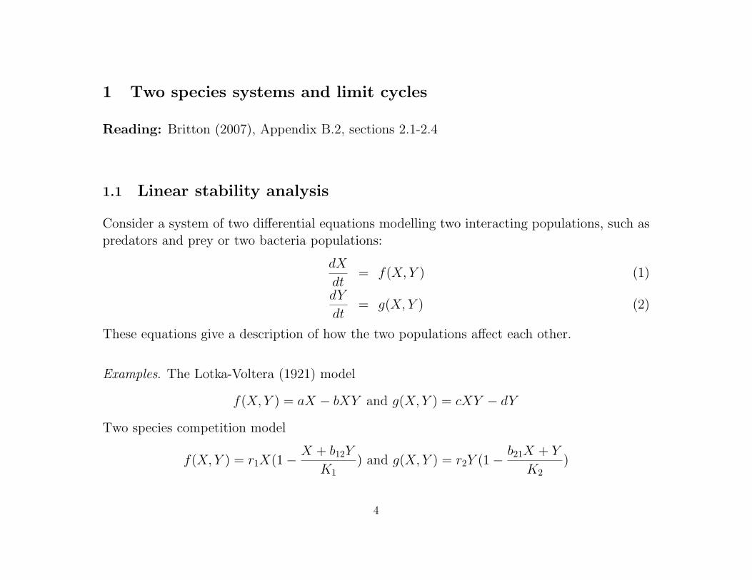
1 Two species systems and limit cycles

Reading: Britton (2007), Appendix B.2, sections 2.1-2.4

1.1 Linear stability analysis

Consider a system of two differential equations modelling two interacting populations, such aspredators and prey or two bacteria populations:

dX

dt= f(X, Y ) (1)

dY

dt= g(X, Y ) (2)

These equations give a description of how the two populations affect each other.

Examples. The Lotka-Voltera (1921) model

f(X, Y ) = aX − bXY and g(X, Y ) = cXY − dY

Two species competition model

f(X, Y ) = r1X(1− X + b12Y

K1) and g(X, Y ) = r2Y (1− b21X + Y

K2)

4

We can linearise models and classify of steady states.

Definition: The nullcline of f , respectively g, is the curve defined by f(X, Y ) = 0, respectivelyg(X, Y ) = 0.

Definition: The steady states of equations 1 and 2 are the constants (X∗, Y∗) such thatf(X∗, Y∗) = 0 and g(X∗, Y∗) = 0. The steady states are the points where the nullclines cross.

”Definition”: A phase plane is a plot in XY space of the nullclines of equations 1 and 2, alongwith steady states and direction arrows indicating the direction of the vector field defined byequations 1 and 2 in the areas separated by the nullclines.

5

In order to determine the stability of our steady states we need to linearise equations 1 and 2.Let X = X∗ + x and Y = Y∗ + y, so that x and y are small perturbations. Then

dx

dt= f(X∗, Y∗) + x

∂f

∂X

∣∣∣∣∣X=X∗,Y=Y∗

+ y∂f

∂Y

∣∣∣∣∣X=X∗,Y=Y∗

+ higher order terms

dy

dt= g(X∗, Y∗) + x

∂g

∂X

∣∣∣∣∣X=X∗,Y=Y∗

+ y∂g

∂Y

∣∣∣∣∣X=X∗,Y=Y∗

+ higher order terms

Since f(X∗, Y∗) = g(X∗, Y∗) = 0,

dx

dt≈ a11x+ a12y

dy

dt≈ a21x+ a22y

where

A =

a11 a12

a21 a22

=

∂f∂X

∣∣∣X=X∗,Y=Y∗

∂f∂Y

∣∣∣X=X∗,Y=Y∗

∂g∂X

∣∣∣X=X∗,Y=Y∗

∂g∂Y

∣∣∣X=X∗,Y=Y∗

We can thus write, x

y

= A

xy

(3)

Now try solution to equation 3 xy

= reλt

6

Therefore,λr = Ar

and0 = (A− λI)r

λ are the eigenvalues of A, while r is the associated eigenvector. Solving

det(A− λI) = 0

gives λ1 and λ2, the eigenvalues and x

y

= c1r1eλ1t + c2r2e

λ2t (4)

where r1 and r2 are the associated eigenvectors and c1 and c2 are constants. Using equation 4we can define the stability of a steady state.

7

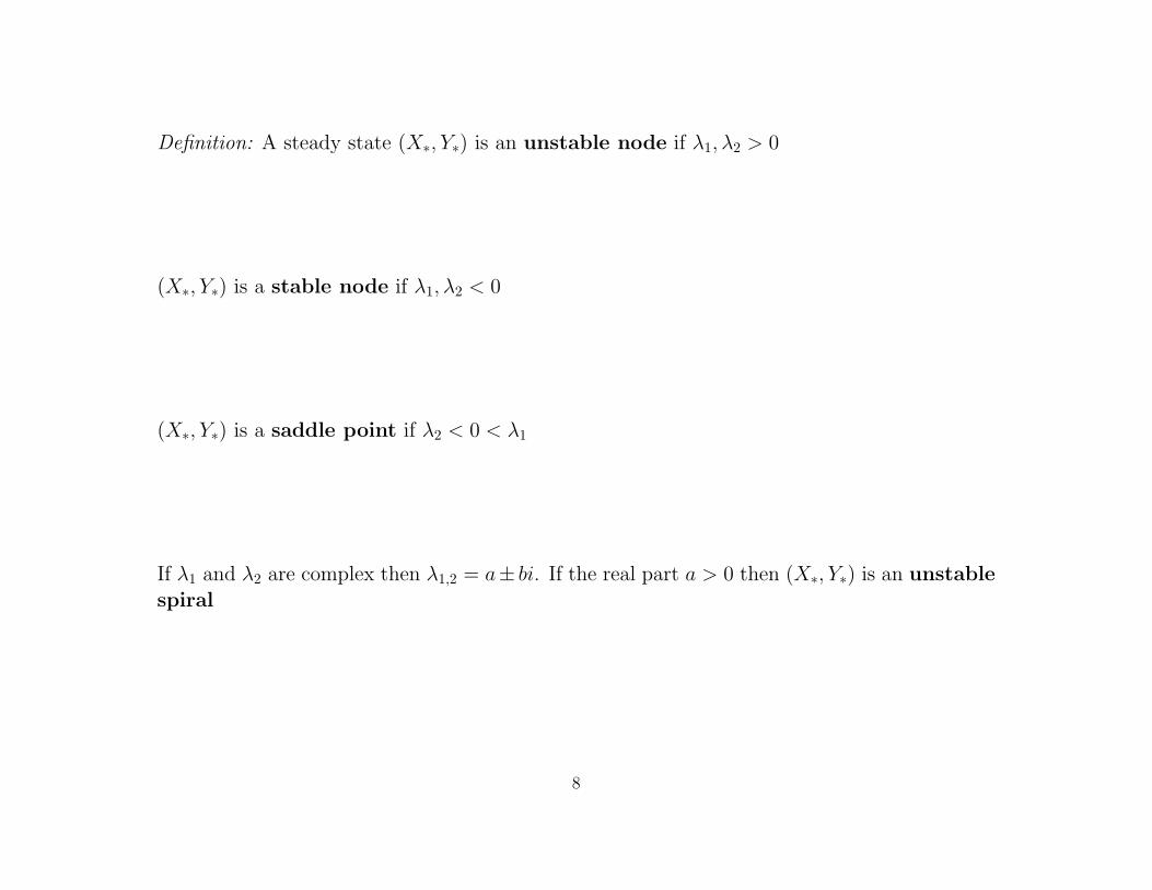
Definition: A steady state (X∗, Y∗) is an unstable node if λ1, λ2 > 0

(X∗, Y∗) is a stable node if λ1, λ2 < 0

(X∗, Y∗) is a saddle point if λ2 < 0 < λ1

If λ1 and λ2 are complex then λ1,2 = a± bi. If the real part a > 0 then (X∗, Y∗) is an unstablespiral

8

If a < 0 then (X∗, Y∗) is a stable spiral

If a = 0 then (X∗, Y∗) is a centre

9

It is often useful to use the fact that the eigenvalues are given by

λ2 − βλ+ γ

where β = a11 + a22 is the trace of A and γ = a11a22 − a12a21 is the determinant

λ =β ±√β2 − 4γ

2

We can plot the stability of the steady states depending on β and γ.

10

Example: The Lotka-Voltera model

dX

dt= aX − bXY (5)

dY

dt= cXY − dY (6)

First non-dimensionalise

u =c

dX , v =

b

aY , τ = at , α = d/a

gives

du

dτ= u(1− v) (7)

dv

dτ= αv(u− 1) (8)

The f-nullclines are at u(1−v) = 0, i.e. u = 0 or v = 1, and the g-nullclines are at αv(u−1) = 0,i.e. v = 0 or u = 1. Thus the steady states (u∗, v∗) are at (0, 0) and (1, 1).

11

We can now draw the phase plane for the model.

12

To determine stability of the steady states we look at the Jacobian matrix:

A =

1− v −uαv α(u− 1)

Evaluated at (0, 0) gives 1 0

0 −α

So λ1 = 1,λ2 = −α. Thus (0, 0) is a saddle point. Evaluated at (1, 1) gives 0 −1

α 0

thus β = 0 and γ = α and (1, 1) is a centre.

13

1.2 Analysing models with periodic behaviour

The techniques from the previous section tell us how to classify each steady state. But theydon’t tell us what happens if we find that none of the steady states are stable. For this we canuse the following theorem.

Poincare-Benedixson Theorem. Let (X, Y ) evolve according to equations 1 and 2. Let (X, Y )be bounded as t → ∞, within a closed region R. As t → ∞, (X(t), Y (t)) tends to a steadystate, or it is or it tends to a periodic solution, such that (X(t), Y (t)) = (X(t + τ), Y (t + τ))for some τ > 0.

This theorem tells us that there are three possibilities for the long term behaviour of (X, Y )when it is bounded. These are illustrated below. Either (X, Y ) goes to a stable steady stateor it is or goes to a periodic solution, known as a limit cycle, within the bounded region R.

14

To show at least one limit cycle exists in a region R with a steady state (X∗, Y∗) we need:

1. (X, Y ) never leaves R.

2. The steady state is unstable.

3. There are no other stable steady states in R.

Complications can arise if there is more than one steady state in a region. The following resultrules out the existence of limit cycles in a region.

Dulac Criterion. Let (X, Y ) evolve according to equations 1 and 2. Let (X, Y ) be bounded ast → ∞, within a closed region R. Suppose there exists a continuously differentiable functionB(X, Y ) such that

∂(Bf)

∂X+∂(Bg)

∂Yis not zero and does not change sign in R. Then there are no periodic orbits in equations 1and 2 in R.

15

1.3 Functional response

In this section we look at a predator-prey model that is an improvement on the Lotka-Volteramodel, given by equations 5 and 6. The problem with the Lokta-Voltera model was that thecycles it produced were very dependent on initial conditions, rather than being a limit cycle.This problem results form assumptions about the rate at which predators attack prey in themodel. The term bXY assumes that individual predators have an unlimited capacity for eatingprey, which is unrealistic. We now derive a more realistic model of predation.

Assume that their are X prey scattered randomly over an area A. Assume that an individualpredator can search an area V per unit time. Assume also that once a predator has founda prey it kills it and takes a time τ to ingest it. Let YS be the number of predators search-ing and YH is the number of predators ingesting. The total number of predators is Y = YS+YH .

We can write the rate of change of searching individuals as

dYSdt

=1

τYH −

V X

AYS

=1

τ(Y − YS)− V X

AYS

At steady state

1

τ(Y − YS∗) =

V X

AYS∗

16

Y

τ=

(1

τ+V X

A

)YS∗

YS∗ =Y

1 + τV XA

So the average number of prey taken per predator per unit time is

V XYS∗AY

=V X/A

1 + τV XA

=1

τ

XAτV +X

Below we plot the rate of attack by predators, known as a type II functional response, as afunction of the number of prey X.

17

1.4 Predator-prey model

Based on this functional response, the predator prey model becomes

dX

dt= aX − 1

τ

XAτV +X

Y

dY

dt=

ε

τ

XAτV +X

Y − dY

This can be further improved by introducing logistic growth for the prey, so they don’t growwithout bound in the absence of predators

dX

dt= a(X −X/K)− 1

τ

XYAτV +X

dY

dt=

ε

τ

XYAτV +X

− dY

We can non-dimensionalise this model to

dx

dt= f(x, y) = x

(1− x/k − uy

1 + x

)(9)

dy

dt= g(x, y) = y

(ux

1 + x− c

)(10)

where k,u and c are constants. We now study this model using phase plane analysis.

18

The nullclines for equation 9 (f) are

x = 0 and y =(1 + x)(1− x/k)

u

and for equation 10 (g) are

y = 0 and x =c

u− cWe draw these nullclines in the phase plane below for four cases: (1) u < c, (2) c < u <

c(1 + 1/k), (3) u = c(1 + 1/k) and (4) u > c(1 + 1/k).

19

There are three possible steady states for equations 9 and 10: (0, 0) (which is a saddle point),(k, 0) (which is stable until u < c(1 + 1/k) and a saddle point otherwise) and c

u− c,u− c(1 + 1/k)

(u− c)2

By calculating the Jacobian, A we can find the trace at this last steady state is

β =c(u(k − 1)− c(k + 1))

(u− c)ku

and the determinant is

γ =c(k(u− c)− c)

ku

From the phase plane in case (4) above, we know that the steady state is a spiral, but could beeither stable or unstable. We can look at when β > 0 to determine stability. Thus the steadystate is stable when u(k − 1)− c(1 + k) < 0 or

u <c(k + 1)

k − 1

20

Below we draw a bifurcation diagram for the predator-prey model for parameter u.

21

There are bifurcations at u = c(1+1/k) (where predator and prey have stable co-existence) andu = c(k+ 1)/(k− 1) (where stable co-existence becomes unstable). When u > c(k+ 1)/(k− 1)we can apply the Poincare-Benedixson theorem (see next section) to show that all trajectoriesapproach a limit cycle. Thus the predator and prey cycle continuously for all initial conditions.

There is a paradox here. We have stable co-existence if

u < c

(1 +

2

k − 1

)

thus increasing the carrying capacity, k, can mean that the steady state becomes unstable! Ina conservation situation it means that giving the prey more resources can lead to predator-preycycles and ultimately less prey.

22