arX

iv:m

ath-

ph/0

0090

29

20 S

ep 2

000

Mathematical Basis for Physical Inference

Albert Tarantola∗ & Klaus Mosegaard†

September 19, 2000

Abstract

While the axiomatic introduction of a probability distribution over a space iscommon, its use for making predictions, using physical theories and prior knowl-edge, suffers from a lack of formalization. We propose to introduce, in the space ofall probability distributions, two operations, the or and the and operation, thatbring to the space the necessary structure for making inferences on possible valuesof physical parameters. While physical theories are often asumed to be analytical,we argue that consistent inference needs to replace analytical theories by proba-bility distributions over the parameter space, and we propose a systematic way ofobtaining such “theoretical correlations”, using the or operation on the results ofphysical experiments. Predicting the outcome of an experiment or solving “inverseproblems” are then examples of the use of the and operation. This leads to a simpleand complete mathematical basis for general physical inference.

∗Institut de Physique du Globe; 4, place Jussieu; F-75005 Paris; France; tarantola@ipgp.jussieu.fr†Niels Bohr Institute for Astronomy, Physics and Geophysics; Dept. of Geophysics; Haraldsgade 6;

DK-2200 Copenhagen N; Denmark; klaus@osiris.gfy.ku.dk

1

Contents

1 Introduction 3

2 The structure of an Inference Space 42.1 Kolmogorov’s concept of probability . . . . . . . . . . . . . . . . . . . . . . 42.2 Inference space . . . . . . . . . . . . . . . . . . . . . . . . . . . . . . . . . 52.3 The interpretation of the or and the and operation . . . . . . . . . . . . . 7

3 Physical parameters 113.1 The noninformative probability density for physical parameters . . . . . . 113.2 Measuring physical parameters . . . . . . . . . . . . . . . . . . . . . . . . . 12

4 Bayesian physical theories 134.1 The “contemplative” point of view . . . . . . . . . . . . . . . . . . . . . . 144.2 The “experimental” point of view . . . . . . . . . . . . . . . . . . . . . . . 144.3 An example of Bayesian theory . . . . . . . . . . . . . . . . . . . . . . . . 154.4 Using a Bayesian physical theory . . . . . . . . . . . . . . . . . . . . . . . 19

5 Discussion and Conclusion 20

6 References and Notes 21

2

1 Introduction

Why has mathematical physics become so universal? Does it allow the proper formulationof usual physical problems? Some reasons explain the popularity of mathematical physics.One reason is practical: mathematical physical theories may condensate a huge numberof experimental results in a few functional relationships. Perhaps more importantly, theserelationships usually have a tremendous power of extrapolation, allowing the prediction ofthe outcome of experiments never performed. Psychologically, this capacity of predictingthe outcome of experiments gives the very satisfactory feeling of “understanding”.

Today, most scientists accept Popper’s (1) point of view that physics advances by pos-tulating mathematical relations between physical parameters. While it is fully recognizedthat physical theories should be confronted with experiments, Popper emphasized thatsucessful predictions, in whatever number, can never prove that a theory is correct, butone single observation that contradicts the predictions of the theory is enough to refute,to falsify the whole theory. He also stressed that these contradictory results are of utter-most importance for the advance of physics. When Michelson and Morley (2) could notfind the predicted difference in the speed of light when the observer changes its velocityrelative to the source, they broke the ground for the replacement of classical by relativisticmechanics.

Physical theories are conceptual models of reality. A good physical theory containssome or all of the following elements:

i) a modelisation of the space-time (for instance, as a four-dimensional continuum, oras a fractal entity)

ii) a modelisation of the objects of the “universe” (for instance, as point particles, oras continuous media)

iii) a recognition of the significant parameters in the experiments to be performed anda precise, operational, definition of these parameters

iv) mathematical relations postulated between these parameters, obtained by tryingto obtain the best fit between observations and theoretical predictions.

While no physics is possible without points (i-iii) above, point (iv), i.e., postulatingfunctional relations between the parameters to be used is not a necessity.

Any physical knowledge is uncertain, and estimation of uncertainties is crucial, forprosaic (e.g., preventing mechanical structures to collapse) as well as ethereal (e.g., usingexperimental results to decide between theories) reasons. The problem we face is thatwhile considerable effort is spent in estimating experimental uncertainties, once a theoryis postulated that is acceptable in view of these uncertainties, usual mathematical physicsreasons as if the theory was exact. For instance, while we can use Gravitation Theory topredict the behaviour of space-time near the big-bang of certain models of the Universe,we have no means of estimating how uncertain are our predictions.

This is more striking when using analytical theories to solve the so-called “inverseproblems” (3–6), where data, a priori information, and “physical theories” have to beused to make inferences about some parameters. The consideration of exact theoriesleads, at best, to inaccurate estimations, at worst, to mathematical inconsistencies (7).

This paper proposes an alternative to the common practice of postulating functionalrelationships between physical parameters. In fact, we propose a mathematical formaliza-

3

tion of pure empiricism, as opposed to mathematical rationalism. Essentially, we suggestto replace functional relationships between physical parameters by well defined probabilitydistributions over the parameter space.

The proposed formalism will, in some sense, only be a sort of “tabulation” of sys-tematically performed experiments. In some aspects it will be less powerful than the oneobtained through the use of analytical theories (it will not be able to extrapolate); in someaspects it will be more powerful (it will be able to properly handle actual uncertainties).

We will show how experiments could be, at least in principle, systematically performedso that a probability distribution in the parameter space is obtained that contains, as ananalytical theory, the observed correlations between physical parameters, but, in addition,contains the full description of the attached uncertainties. We will also explain how,once such a theoretical probability distribution has been obtained, we can use it to makepredictions —that will have attached uncertainties— or to use data to solve general inverseproblems.

To fulfill this project we need to complete classical probability theory. Kolmogorov (8)proposed an axiomatic introduction of the notion of probability distribution over a space.The definition of conditional probability is then the starting point for doing inferences,as, for instance, through the use of the Bayes theorem. But the space of all probabilitydistributions (over a given space) lacks structure. We argue below that there are twonatural operations, the or and the and operation, to be defined over the probabilitydistributions, that create the necessary structure: that of an inference space. We willsee that while the or operation corresponds to an obvious generalization of “makinghistograms” from observed results, the and operation is just the right generalization ofthe notion of conditional probability.

2 The structure of an Inference Space

Before Kolmogorov (8), probability calculus was made using the intuitive notions of“chance” or “hazard”. Kolmogorov’s axioms clarified the underlying mathematical struc-ture and brought probability calculus inside well defined mathematics. In this section wewill recall these axioms. Our opinion is that the use in physical theories (where we haveinvariance requirements) of probability distributions, through the notions of conditionalprobability or the so-called Bayesian paradigm suffers today from the same defects asprobability calculus suffered from before Kolmogorov. To remedy this, we introduce inthis section, in the space of all probability distributions, two logical operations (or andand) that give the necessary mathematical structure to the space.

2.1 Kolmogorov’s concept of probability

A point x , that can materialize itself anywhere inside a domain D , may be realized,for instance, inside A , a subdomain of D . The probability of realization of the pointis completely described if we have introduced a probability distribution (in Kolmogorov’s[8] sense) on D , i.e., if to every subdomain A of D we are able to associate a realnumber P (A) , called the probability of A , having the three properties:

4

• For any subdomain A of D , P (A) ≥ 0 .• If Ai and Aj are two disjoint subsets of D , then, P (Ai ∪Aj) = P (Ai) + P (Aj) .• For a sequence of events A1 ⊇ A2 ⊇ · · · tending to the empty set, we have P (Ai)→ 0 .

We will not necessarily assume that a probability distribution is normed to unity( P (D) = 1 ). Although one refers to this as a measure, instead of a probability, we willnot use this distinction. Sometimes, our probability distributions will not be normalizableat all ( P (D) =∞ ). We can only then compute the relative probabilities of subdomains.

These axioms apply to probability distributions over discrete or continuous spaces.Below, we will consider probability distributions over spaces of physical parameters, thatare continuous spaces. Then, a probability distribution is represented by a probabilitydensity (note [9] explains the difference between a probability density and a volumetricprobability).

In the next section, given a space D , we will consider different probability dis-tributions P , Q . . . Each probability distribution will represent a particular state ofinformation over D . In what follows, we will use as synonymous the terms “probabilitydistribution” and “state of information”.

2.2 Inference space

We will now give a structure to the space of all the probability distributions over a givenspace, by introducing two operations, the or and the and operation. This contrastswith the basic operations introduced in deductive logic, where the negation (“not”),nonexistent here, plays a central role. In what follows, the or and the and operation willbe denoted, symbollically, by ∨ and ∧ . They are assumed to satisfy the set of axiomshere below.

The first axiom states that if an event A is possible for (P or Q) , then the eventis either possible for P or possible for Q (which his is consistent with the usual logicalsense for the “or”): For any subset A , and for any two probability distributions P andQ , the or operation satisfies

(P ∨Q) (A) 6= 0 =⇒ P (A) 6= 0 or Q(A) 6= 0 ,

the word “or” having here its ordinary logical sense.The second axiom states that if an event A is possible for (P and Q) , then the

event is possible for both P and Q (which is consistent with the usual logical sense forthe “and”): For any subset A , and for any two probability distributions P and Q ,the and operation satisfies

(P ∧Q) (A) 6= 0 =⇒ P (A) 6= 0 and Q(A) 6= 0 ,

the word “and” having here its ordinary logical sense.The third axiom ensures the existence of a neutral element, that will be interpreted

below as the probability distribution carrying no information at all: There is a neutralelement, M for the and operation, i.e., it exists a M such that for any probabilitydistribution P and for any subset A ,

(M ∧ P ) (A) = (P ∧M) (A) = P (A) .

5

The fourth axiom imposes that the or and the and operations are commutative andassociative, and, by analogy with the algebra of propositions of ordinary logic, have adistributivity property: the and operation is distributive with respect to the or operation.

The structure obtained when furnishing the space of all probability distributions (overa given space D ) with two operations or and and, satisfying the given axioms constituteswhat we propose to call an inference space.

These axioms do not define uniquely the operations. Let µ(x) be the particularprobability density representing M , the neutral element for the and operation, andlet p(x), q(x) . . . be the probability densities representing the probability distributionsP,Q . . . Using the notations (p ∨ q)(x) and (p ∧ q)(x) for the probability densitiesrepresenting the probability distributions P ∨Q and P ∧Q respectively, one realizationof the axioms (the one we will retain) is given by

(p ∨ q)(x) = p(x) + q(x) ; (p ∧ q)(x) =p(x) q(x)

µ(x), (1)

where one should remember that we do not impose to our probability distributions to benormalized.

The structure of an inference space, as defined, contains other useful solutions. Forinstance, the theory of fuzzy sets (10) uses positive functions p(x), q(x) . . . quite similarto probability densities, but having a different interpretation: the are normed by thecondition that their maximum value equals one, and are interpreted as the “grades ofmembership” of a point x to the “fuzzy sets” P,Q . . . . The operations or and and

correspond then respectively to the union and intersection of fuzzy sets, and to thefollowing realization of our axioms:

(p ∨ q)(x) = max(p(x), q(x)) ; (p ∧ q)(x) = min(p(x), q(x)) , (2)

where the neutral element for the and operation (intersection of fuzzy sets) is simply thefunction µ(x) = 1 .

While fuzzy set theory is an alternative to classical probability (and is aimed at thesolution of a different class of problems), our aim here is only to complete the classicalprobability theory. As explained below the solution given by equations 1 correspond tothe natural generalisation of two fundamental operations in classical probability theory:that of “making histograms” and that of taking “conditional probabilities”. To simplifyour language, we will sometimes use this correspondence between our theory and thefuzzy set theory, and will say that the or operation, when applied to two probabilitydistributions, corresponds to the union of the two states of information, while the and

operation corresponds to their intersection.It is easy to write some extra conditions that distinguish the two solutions given by

equations 1 and 2. For instance, as probability densities are normed using a multiplicativeconstant (this is not the case with the grades of membership in fuzzy set theory), it makessense to impose the simplest possible algebra for the multiplication of probability densitiesp(x), q(x) . . . by constants λ, µ . . . :

[(λ+ µ)p] (x) = (λp ∨ µp) (x) ; [λ(p ∧ q)] (x) = (λp ∧ q) (x) = (p ∧ λq) (x) . (3)

6

This is different from finding a (minimal) set of axioms characterizing (uniquely) theproposed solution, which is an open problem.

One important property of the two operations or and and just introduced is that ofinvariance with respect to a change of variables. As we consider probability distributionover a continuous space, and as our definitons are independent of any choice of coordinatesover the space, it must happen that we obtain equivalent results in any coordinate system.Changing for instance from the coordinates x to some other coordinates y , will changea probability density p(x) to p̃(y) = p(x) |∂x/∂y| . It can easily be seen (11) thatperforming the or or the and operation, then changing variables, gives the same resultthan first changing variables, then, performing the or or the and operation.

Let us mention that the equivalent of equations 1 for discrete probability distributionsis:

(p ∨ q)i = pi + qi ; (p ∧ q)i =pi qiµi

. (4)

Although the or and and notions just introduced are consistent with classical logic,they are here more general, as they can handle states of information that are more subtlethan just the “possible” or “impossible” ones.

2.3 The interpretation of the or and the and operation

If an experimenter faces realizations of a random process and wants to investigate theprobability distribution governing the process, he may start making histograms of therealizations. For instance, for realizations of a probability distribution over a continuousspace, he will obtain histograms that, in some sense, will approach the probability densitycorresponding to the probability distribution.

A histogram is typically made by dividing the working space into cells, and by countinghow many realizations fall inside each cell. A more subtle approach is possible. First,we have to understand that, in the physical sciences, when we say “a random point hasmaterialized in an abstract space”, we may mean something like “this object, one amongmany that may exist, vibrates with some fixed period; let us measure as accurately aspossible its period of oscillation”. Any physical measure of a real quantity will haveattached uncertainties. As explained in section 3.2, this means that when, mathematicallyspeaking, we measure “the coordinates of a point in an abstract space” we will not obtaina point, but a state of information over the space, i.e., a probability distribution.

If we have measured the coordinates of many points, the results of each measure-ment will be described by a probability density pi(x) . The union of all these, i.e., theprobability density

(p1 ∨ p2 ∨ . . .) (x) =∑i

pi(x) (5)

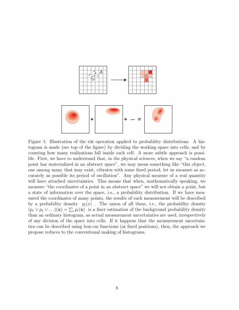
is a finer estimation of the background probability density than an ordinary histogram, asactual measurement uncertainties are used, irrespectively of any division of the space intocells. If it happens that the measurement uncertainties can be described using box-carfunctions at fixed positions, then, the approach we propose reduces to the conventionalmaking of histograms. This is illustrated in figure 1.

7

+ + =...

...

...

... ...

.

Figure 1: Illustration of the or operation applied to probability distributions. A his-togram is made (see top of the figure) by dividing the working space into cells, and bycounting how many realizations fall inside each cell. A more subtle approach is possi-ble. First, we have to understand that, in the physical sciences, when we say “a randompoint has materialized in an abstract space”, we may mean something like “this object,one among many that may exist, vibrates with some fixed period; let us measure as ac-curately as possible its period of oscillation”. Any physical measure of a real quantitywill have attached uncertainties. This means that when, mathematically speaking, wemeasure “the coordinates of a point in an abstract space” we will not obtain a point, buta state of information over the space, i.e., a probability distribution. If we have mea-sured the coordinates of many points, the results of each measurement will be describedby a probability density pi(x) . The union of all these, i.e., the probability density(p1 ∨ p2 ∨ . . .)(x) =

∑i pi(x) is a finer estimation of the background probability density

than an ordinary histogram, as actual measurement uncertainties are used, irrespectivelyof any division of the space into cells. If it happens that the measurement uncertain-ties can be described using box-car functions (at fixed positions), then, the approach wepropose reduces to the conventional making of histograms.

8

0. 2. 4. 6. 8. 10.0.

2.

4.

6.

8.

10.

0. 2. 4. 6. 8. 10.0.

2.

4.

6.

8.

10.

0. 2. 4. 6. 8. 10.0.

2.

4.

6.

8.

10.

0. 2. 4. 6. 8. 10.0.

2.

4.

6.

8.

10.

0. 2. 4. 6. 8. 10.0.

2.

4.

6.

8.

10.

P( )

Q( )

P( |B)

.

.

.. (P/\Q)( )

P(A∩B)P(B)

P(A|B) = (p/\q)(x) =(x)

p(x) q(x)

B

mu

Figure 2: Illustration of the and operation applied to probability distributions. Thisfigure explains that our definition of the and operation is a generalization of the notion ofconditional probability. A probability distribution P ( · ) is represented (left of the figure)by its probability density. To any region A of the plane, it associates the probabilityP (A) . If a point has been realized following the probability distribution P ( · ) and weare given the information that, in fact, the point is “somewhere” inside the region B , thenwe can update the prior probability P ( · ) , replacing it by the conditional probabilityP ( · |B) = P ( · ∩ B)/P (B) . It equals P ( · ) inside B and is zero outside (center ofthe figure). If instead of the hard constraint x ∈ B we have a soft information about thelocation of x , represented by the probability distribution Q( · ) (right of the figure), theintersection of the two states of information P and Q gives a new state of information(here, µ(x) is the probability density representing the state of null information, and, tosimplify the figure, has been assumed to be constant). The comparison of the right withthe center of the figure shows that the and operation generalizes the notion of conditionalprobability. In the special case where the probability density representing the second stateof information, Q( · ) , equals the null information probability density inside the domainB and is zero outside, then, the notion of intersection of states of information exactlyreduces to the notion of conditional probability.

9

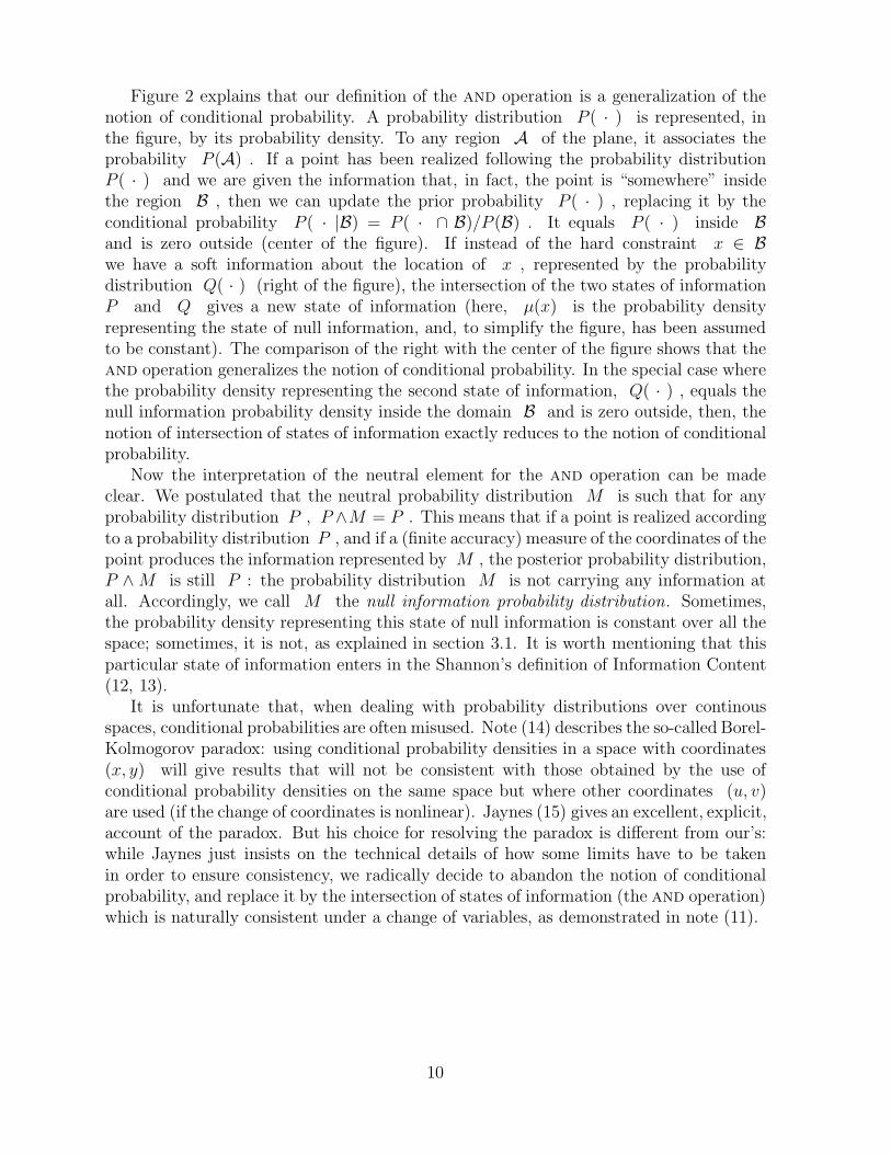
Figure 2 explains that our definition of the and operation is a generalization of thenotion of conditional probability. A probability distribution P ( · ) is represented, inthe figure, by its probability density. To any region A of the plane, it associates theprobability P (A) . If a point has been realized following the probability distributionP ( · ) and we are given the information that, in fact, the point is “somewhere” insidethe region B , then we can update the prior probability P ( · ) , replacing it by theconditional probability P ( · |B) = P ( · ∩ B)/P (B) . It equals P ( · ) inside Band is zero outside (center of the figure). If instead of the hard constraint x ∈ Bwe have a soft information about the location of x , represented by the probabilitydistribution Q( · ) (right of the figure), the intersection of the two states of informationP and Q gives a new state of information (here, µ(x) is the probability densityrepresenting the state of null information, and, to simplify the figure, has been assumedto be constant). The comparison of the right with the center of the figure shows that theand operation generalizes the notion of conditional probability. In the special case wherethe probability density representing the second state of information, Q( · ) , equals thenull information probability density inside the domain B and is zero outside, then, thenotion of intersection of states of information exactly reduces to the notion of conditionalprobability.

Now the interpretation of the neutral element for the and operation can be madeclear. We postulated that the neutral probability distribution M is such that for anyprobability distribution P , P ∧M = P . This means that if a point is realized accordingto a probability distribution P , and if a (finite accuracy) measure of the coordinates of thepoint produces the information represented by M , the posterior probability distribution,P ∧M is still P : the probability distribution M is not carrying any information atall. Accordingly, we call M the null information probability distribution. Sometimes,the probability density representing this state of null information is constant over all thespace; sometimes, it is not, as explained in section 3.1. It is worth mentioning that thisparticular state of information enters in the Shannon’s definition of Information Content(12, 13).

It is unfortunate that, when dealing with probability distributions over continousspaces, conditional probabilities are often misused. Note (14) describes the so-called Borel-Kolmogorov paradox: using conditional probability densities in a space with coordinates(x, y) will give results that will not be consistent with those obtained by the use ofconditional probability densities on the same space but where other coordinates (u, v)are used (if the change of coordinates is nonlinear). Jaynes (15) gives an excellent, explicit,account of the paradox. But his choice for resolving the paradox is different from our’s:while Jaynes just insists on the technical details of how some limits have to be takenin order to ensure consistency, we radically decide to abandon the notion of conditionalprobability, and replace it by the intersection of states of information (the and operation)which is naturally consistent under a change of variables, as demonstrated in note (11).

10

3 Physical parameters

Crudely speaking, a physical parameter is anything that can be measured. For a physicalparameter, like a temperature, an electric field, or a mass, can only be defined by pre-scribing the experimental procedure that will measure it. Cook (16) discusses this pointwith lucidity.

The theory to be developed in this article will be illustrated by the analysis of objectsthat have a characteristic length, L , affected by phenomena that have a characteristicperiod, T . A measurement of a parameter is performed by realizing the conventional unit(i.e., the meter for a length, the second for a duration) and by comparing the parameterto the unit. We have then to turn to the definition of the units of time duration and oflength.

At present, the second is defined as the duration of 9 192 631 770 periods of theradiation corresponding to the transition between the two hyperfine levels of the groundstate of the cæsium-133 atom. Practically this means that a beam of cæsium-133 atomsare submitted to an electromagnetic field of adjustable frequency: when the imposedfrequency is such that it causes the transition between the two hyperfine levels of theground state of the atoms, the standard of frequency (and, thus, of period) has beenrealised.

Until 1991, the unit of length used to be defined independently of that of time duration.Now the meter is connected to the second by defining the value of the velocity of lightas c = 299 792 458 m s−1. This means, in fact, that lengths are measured by measuringthe time it takes light to traverse them (and then, converting to distance through thisconventional value of c ).

3.1 The noninformative probability density for physical param-eters

Once a physical parameter has been defined, it is possible to associate to it a particularprobability distribution, that will represent, when making a measurement, the absence ofinformation on the possible outcome of the experiment.

Assume that, furnished with our definition of the unit of time duration, we wish tomeasure the period of some object. It can be the period of a rotating galaxy, or theperiod of a XVII-th century pendulum, or the period of a vibrating molecule: we do notknow yet. Let us denote by p(T ) the probability density representing this state of totalignorance. The frequency ν associated to the period T is ν = 1/T . ¿From p(T ) wecan, using the general rule of change of variables, deduce the probability density for thefrequency: q(ν) = p(T ) |dT/dν| = p(T )/ν2 .

Now, the definition of the unit of time duration is undistinguishable from the definitionof the unit of frequency. In fact, when trying to define the standard of time we said “whenthe imposed frequency is such that is causes the transition between the two hyperfinelevels of the ground state of the atoms, the standard of frequency has been realised”,which shows how closely related are the reciprocal parameters period-frequency: we cannot define the unit second without defining, at the same time, the unit Hertz .

We find here, at a very fundamental level, the class of reciprocal parameters analyzed

11

by Harold Jeffreys (17). As he argued, the null information probability density must havethe same form for the two parameters, i.e., p(·) and q(·) must be the same function.Then, the constraint q(ν) = p(T )/ν2 , seen above, gives, up to a multiplicative constant,the solution

p(T ) =1

T; q(ν) =

1

ν. (6)

The range of time durations (or of periods) considered in physics spans many ordersof magnitude (from periods of atomic objects to cosmological periods). Physicists thenoften use a logarithmic scale, defining, for instance, T ∗ = log(T/T0) and ν∗ = log(ν/ν0) ,where the two constants ν0 and T0 can be arbitrary (18). Transforming the probabilitydensities in 6 to the logarithmic variables gives p∗(T ∗) = 1 and q∗(ν∗) = 1 . The loga-rithmic variables (that take values on all the real line) have a constant probability density.This, is fact, is the deep interpretation of the 1/x probability densities in equations 6.The particular variables for which the probability density representing the state of nullinformation is a constant over all the space can be named Cartesian: they are more “nat-ural” than others, as are the usual Cartesian coordinates in Euclidean spaces (19). Thatthese “Cartesian” variables are not only more natural, but also more practical than othervariables, can be understood by considering that manufacturers of pianos space notes withconstant increments not of frequency, but of the associated logarithmic variable.

We have seen that the definition of length is today related to that of time durationthrough the velocity of light. We could say that the electromagnetic wave of the radia-tion that defines the unit of time, defines, through its wavelength, the unit of distance.But, here again, we have a perfect symmetry between the wavelength and its inverse,the wavenumber. This is why we take the function h(L) = 1/L to describe the nullinformation probability density for the length of an object (20).

3.2 Measuring physical parameters

To define the experimental procedure that will lead to a “measurement” we need toconceptualize the objects of the “universe”: do we have point particles or a continuousmedium? Any instrument that we can build will have finite accuracy, as any manufactureis imperfect. Also, during the measurement act, the instrument will always be submittedto unwanted sollicitations (like uncontrolled vibrations).

This is why, even if the experimenter postulates the existence of a well defined, “truevalue”, of the measured parameter, she/he will never be able to measure it exactly. Carefulmodeling of experimental uncertainties is not easy, Sometimes, the result of a measurementof a parameter p is presented as p = p0 ± σ , where the interpretation of σ may bediverse. For instance, the experimenter may imagine a bell-shaped probability densityaround p0 representing her/his state of information “on the true value of the parameter”.The constant σ can be the standard deviation (or mean deviation, or other estimator ofdispersion) of the probability density used to model the experimental uncertainty.

In part, the shape of this probability density may come from histograms of observedor expected fluctuations. In part, it will come from a subjective estimation of the de-fects of the unique pieces of the instrument. We postulate here that the result of anymeasurement can, in all generality, be described by defining a probability density over

12

the measured parameter, representing the information brought by the experiment on the“true”, unknowable, value of the parameter. The official guidelines for expressing uncer-tainty in measurement, as given by the International Organization for Standardization(ISO) and the National Institute of Standards and Technology (21) although stressingthe special notion of standard deviation, are consistent with the possible use of generalprobability distributions to express the result of a measurement, as advocated here.

Any shape of the density function is not acceptable. For instance, the use of a Gaussiandensity to represent the result of a measurement of a positive quantity (like an electricresistivity) would give a finite probability for negative values of the variable, which isinconsistent (a lognormal probability density, on the contrary, could be acceptable).

In the event of an “infinitely bad measurement” (like when, for instance, an unexpectedevent prevents, in fact, any meaningful measure) the result of the measurement should bedescribed using the null information probability density introduced above. In fact, whenthe density function used to represent the result of a mesurement has a parameter σdescribing the “width” of the function, it is the limit of the density function for σ →∞that should represent a measurement of infinitely bad quality. This is consistent, forinstance, with the use of a lognormal probability density for a parameter like an electricresisitivity r , as the limit of the lognormal for σ → ∞ is the 1/r function, which isthe right choice of noninformative probability density for r .

Another example of possible probability density to represent the result of a measure-ment of a parameter p is to take the noninformative probability density for p1 < p < p2

and zero outside. This fixes strict bounds for possible values of the parameter, and tendsto the noninformative probability density when the bounds tend to infinity.

The point of view proposed here will be consistent with the the use of “theoreticalparameter correlations” as proposed in section 4.4, so that there is no difference, fromour point of view, between a “simple measurement” and a measurement using physicaltheories, including, perhaps, sophisticated inverse methods.

4 Bayesian physical theories

Physical “laws” prevent us from setting arbitrarily some physical parameters. For in-stance, we can set the length of a tube where a free fall experiment will be performed,and we can also decide on the place and time of the experiment, but the time duration ofthe free fall is “imposed by Nature”. Physics in much about the analysis of these physicalcorrelations between parameters.

Typically, a set i of independent parameters is identified, and experiments are per-formed in order to measure the values of a set d of dependent parameters (22). Analyticalphysical theories try then to express the result of the observations by a functional rela-tionship d = d(i) . In fact, saying that the independent parameters are “set” and thedependent parameters “measured” is an oversimplification, as all the parameters must bemeasured. And, as discussed in the previous section, uncertainties are present in everymeasurement. The values of the parameters that are set (the independent parameters) arenever known exactly. The measures of the dependent parameters have always uncertain-ties attached. Assume we have made a large number of experiments, that show how the

13

dependent parameters correlate with the independent ones. Within the error bars of theexperimental results it will always be possible to fit an infinity of functional relationshipsof the form d = d(i) . Adding more experimental points may help to discard some ofthe “theories”, but there will always remain an infinity of them.

We formalize this fact at a fundamental level, by replacing the need of a functionalrelationship by the use of a probability distribution in the space of all the parametersconsidered, representing the actual information we may have. Not only this point of viewcorresponds to a certain philosophy of physics, it also leads —as discussed below— to theonly consistent formalism we know that is able to predict values of possible observationsand of the attached uncertainties.

To be complete, we consider two cases where we may wish to analyze the physicalcorrelations between parameters. The first case is when a repetitive phenomenon takesplace spontaneously. The second case correspond to the case when an experimenterprompts a physical phenomenon, using an experimental arrangement.

4.1 The “contemplative” point of view

Consider an astronomer trying to analyze the “relationship” between the initial magni-tude m of shooting stars and the total distance ∆ traveled by the meteors on the skybefore disintegration. Each shooting star naturally appearing on the sky will allow onemeasurement of the two parameters m and ∆ to be performed (and possibly othersignificant parameters). As discussed above, each result of a measurement will be repre-sented by a probability density. Let θi(m,∆) be the probability density representing theinformation obtained on the parameters m and ∆ of the i-th shooting star.

When a large enough number of shooting starts has been observed, the correlationbetween the parameters m and ∆ is perfectly described by the probability densityobtained by applying the or operation (as defined by the first of equations 1) to theprobability distributions represented by θ1(m,∆), θ2(m,∆), . . . , i.e., by the probabilitydensity θ(m,∆) =

∑i θi(m,∆) . If, more generally, the observed parameters are generi-

cally represented by x , and the result of the i-th experiment, by the probability densityθi(x) , then,

θ(x) =∑i

θi(x) . (7)

The utility of this probability density will be explained in section 4.4.

4.2 The “experimental” point of view

Here, the independent parameters i are “set”, and the dependent parameters d mea-sured. This case can be reduced to the previous case (the “contemplative” one) providedthat the independent parameters i are “randomly generated” according to some refer-ence probability distribution, as, for instance, the null information probability distributiondiscussed in section 3.1 (this guaranteeing, in particular, that any possible region of thespace of independent parameters will eventually be sampled).

As above, if θi(i,d) is the probability density representing the information on i andd obtained from the i-th experiment, after a large enough number of experiments has

14

been performed, the correlations between the dependent and the independent parametersare described by the probability density θ(i,d) =

∑i θi(i,d) . In general, if the whole

set of parameters is generically represented by x = {i,d} , and the result of the i-thexperiment, by the probability density θi(x) , then equation 7 holds again.

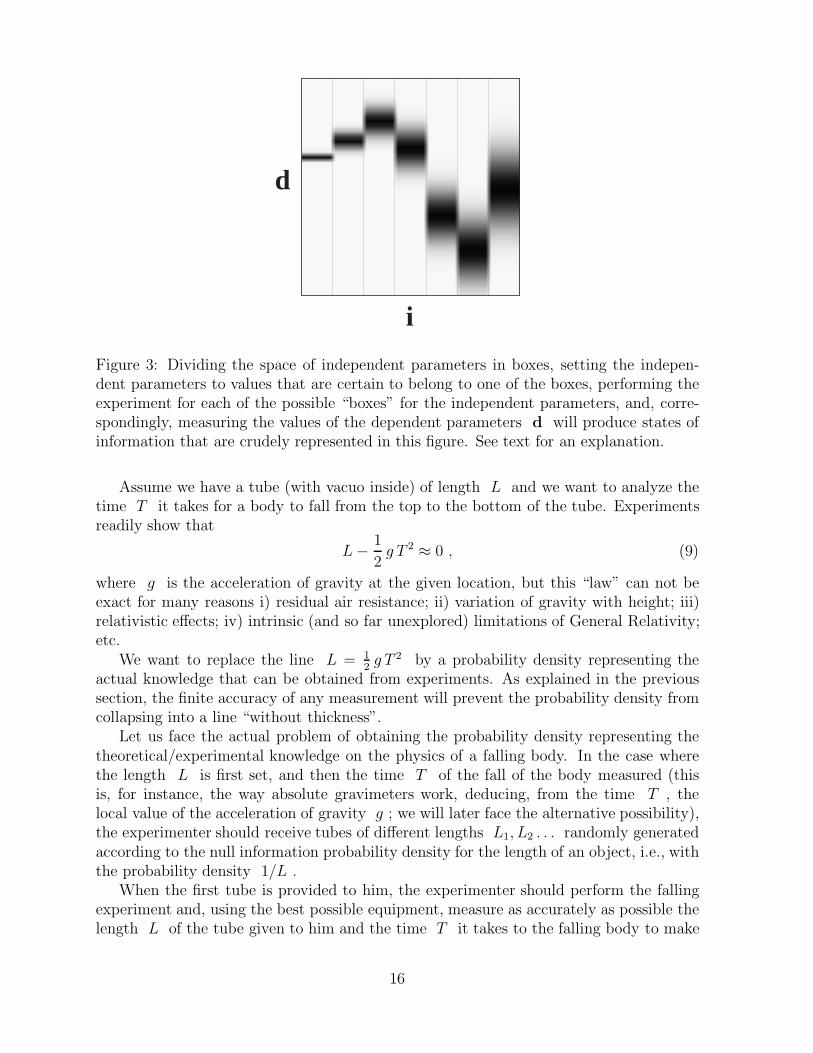
We have here assumed that the values of the independent parameters are set ran-domly according to their null information probability density. This directly leads tothe “Bayesian theory” θ(i,d) (this terminology being justified in section 4.4). A secondoption consists in defining physical correlations between parameters as a conditional prob-ability density for the dependent parameters, given the independent parameters, θ(d|i) ,but for the reasons explained elsewhere (14) the notion of conditional probability density,although a valid mathematical definition, is not of direct use for handling experimentalresults, unless enough care is taken. Assume, for instance, that the space of independentparameters is divided in boxes (multidimensional “intervals”) and that the independentparameters can be set to values that are certain to belong to one of the boxes. Performingthe experiment for each of the possible “boxes” for the independent parameters, and, cor-respondingly, measuring the values of the dependent parameters d will produce statesof information that are crudely represented in figure 3. This collection of states of infor-mation correspond to the conditional probability density θ(d|i) . The joint probabilitydensity in the (i,d) space that carries this information without carrying any informa-tion about the independent parameters (what we wish to call the “Bayesian theory”) isthen the product of the conditional probability density θ(d|i) by the null informationprobability density for the independent paremeters, say µI(i) , i.e., the probability density

θ(i,d) = θ(d|i)µI(i) . (8)

To be more accurate, if, in each experiment, the only thing we know about the independentparameters is the box where their value belongs, the measurement produces a probabilitydensity in the (i,d) space, say θi(i,d) , that equals the product of a probability densityover d (describing the result of the measurement of the dependent parameters) timesa probability density that equals zero outside the box and equals the null informationprobability density inside the box. Applying the or operation to all these probabilitydensitues will also give the result of equation 8.

Interpreting the conditional probability density θ(d|i) as simply putting some “errorbars” around some “true functional relationship” d = d(i) , that will always escape toour knowledge, or assuming that the experimental knowledge θ(d|i) represents is the“real thing”, and that there is no necessity of postulating the existence of a functionalrelationship, is a methaphysical question that will not change the manner of doing physicalinference. As explained in section 4.4, inference will combine this “theoretical knowledge”represented by θ(i,d) with further experiments using the and operation.

4.3 An example of Bayesian theory

The discussion on the noninformative priors, in section 3.1, was made without referenceto a particular kind of object to be investigated. Let us now turn to analyze the physicsof the fall of objects at the surface of the Earth.

15

d

i

Figure 3: Dividing the space of independent parameters in boxes, setting the indepen-dent parameters to values that are certain to belong to one of the boxes, performing theexperiment for each of the possible “boxes” for the independent parameters, and, corre-spondingly, measuring the values of the dependent parameters d will produce states ofinformation that are crudely represented in this figure. See text for an explanation.

Assume we have a tube (with vacuo inside) of length L and we want to analyze thetime T it takes for a body to fall from the top to the bottom of the tube. Experimentsreadily show that

L− 1

2g T 2 ≈ 0 , (9)

where g is the acceleration of gravity at the given location, but this “law” can not beexact for many reasons i) residual air resistance; ii) variation of gravity with height; iii)relativistic effects; iv) intrinsic (and so far unexplored) limitations of General Relativity;etc.

We want to replace the line L = 12g T 2 by a probability density representing the

actual knowledge that can be obtained from experiments. As explained in the previoussection, the finite accuracy of any measurement will prevent the probability density fromcollapsing into a line “without thickness”.

Let us face the actual problem of obtaining the probability density representing thetheoretical/experimental knowledge on the physics of a falling body. In the case wherethe length L is first set, and then the time T of the fall of the body measured (thisis, for instance, the way absolute gravimeters work, deducing, from the time T , thelocal value of the acceleration of gravity g ; we will later face the alternative possibility),the experimenter should receive tubes of different lengths L1, L2 . . . randomly generatedaccording to the null information probability density for the length of an object, i.e., withthe probability density 1/L .

When the first tube is provided to him, the experimenter should perform the fallingexperiment and, using the best possible equipment, measure as accurately as possible thelength L of the tube given to him and the time T it takes to the falling body to make

16

the distance. This would provide him with a probability density θ1(L, T ) representing hisknowledge of the realized value of the parameters. There is no reason for the uncertaintieson L and T , as described by this probability density, to be independent. When a secondtube, with random length, is provided to him, he should perform again the experimentand obtain a second probability density θ2(L, T ) . As already explained, the “Bayesiantheory” corresponding to these experiments is then the union (in the sense defined above)of all the states of information obtained in all the individual experiments, when theirnumber tends to infinity:

θ(L, T ) =∞∑i=1

θi(L, T ) . (10)

Figure 4 schematizes the sort of probability density such a method would produce (23).We have explored the case where the length L of the tube is first set and, then,

the falling experiment is performed, measuring the time T . The alternative is to fixthe time duration T first and, then, to perform the the falling experiment, measuringthe length L the falling body has traveled in that time. The two sorts of experimentsare not identical, as the type of measurements performed will be different and will leadto different uncertainties. In this case, the experimenter is provided with time durationsT1, T2 . . . randomly selected according to the null information probability density for theperiod of a process, and obtains probability densities ϑ1(L, T ), ϑ2(L, T ) . . . representingthe results of the measurements. The union of all these states of information

ϑ(L, T ) =∞∑i=1

ϑi(L, T ) , (11)

would provide the “Bayesian theory” corresponding to that sort of experiment.There is no reason for the two “Bayesian theories” thus obtained to be identical, as they

correspond to a different type of experiment. We are then faced with the conclusion thatthe replacement of an analytical equation by a probability density will lead to probabilitydensities attached to the precise experiment being performed. In fact, this is not sodifferent to what would have been obtained when seeking for a functional relationship,as the “best fitting curve” for the first kind of experiments may not be the “best fitting”one for the second kind of experiments.

The formation of a “Bayesian theory” here made by summing small distributions (“his-togramming”) can be understood in two ways. First, we could perfectly well proceed inthis way in practice, performing systematic measurements of parameter correlations, us-ing the best avalilable equipment. Alternatively, we can understand the proposed methodas a thought experiment helping to clarify what “theoretical uncertainties” can be. Theseuncertainties can then be modeled using standard distributions (Gaussian, double expo-nential. . . ) in such a way that usable but still realistic probability distributions in theparameter space can be defined and used as “Bayesian theories”, as in the example shownin note (23).

We will conclude this section with two remarks. First, it is not possible to samplea probability distribution that can not be normalized, as it is usually the case for thenoninformative probabilities, like, for positive x , the 1/x distribution. Then, practicallower and upper bounds have to be used. Second, the number of experimental “points”

17

L

T

Figure 4: The free fall of an object inside a tube of length L takes some time duration T .Experiments show that there is a good correlation between L and T : with a goodapproximation, L − 1

2g T 2 ≈ 0 . An analitycal expression like L = 1

2g T 2 can not

be exact (any analytical theory is just an approximation of reality). An examination ofthe real experiments made to obtain the “theory” shows the presence of uncompressibleuncertainties. Using the approach developed here, the existing correlations between Land T are represented by a probability density which replaces the classical notion ofanalytic theory. If, at some scale, these correlations may seem well described by ananalytical expression (here, in the top figure, by a line), succesive magnifications (middleand bottom) end up by showing the actual size of the “theoretical uncertainties”. Inthis example we have assumed that measurements of lengths and of time durations haveconstant relative errors (grossly exaggerated in this schematic drawing). The thickness ofthis theoretical distribution is of importance for: i) solving, in a mathematical consistentmanner physical inference problems, and ii) accurately computing uncertainties betweenphysical parameters, as, for instance, when predicting data values or when solving inverseproblems.

18

that have to be used in order to have a good practical approximation of a “Bayesiantheory” depends on the accuracy of the measurements. Enough experiments have tobe done so that the sum in equations 10 and 11 is smooth enough. The sharper theexperimental design, the more experiments we will need (and the mode detail we willhave).

4.4 Using a Bayesian physical theory

Assume that enough experiments have been made, by skilled people, using the best avail-able equipment, following the guidelines of the previous section, so that the “Bayesiantheory” θ(L, T ) is available. Now a new tube is given to us, whose length has beenrandomly generated according to the null information probability density, 1/L . Weperform the falling experiment, perhaps with a more modest equipment than that used toobtain the Bayesian theory, and measure the two parameters L and T , the result of themeasurement being described by the state of information ρ(L, T ) . How can we combinethis information with the Bayesian theory, so that we can ameliorate our knowledge on Land T ? We are exactly here in the situation where the notion of conditional probability(in fact, our generalization of it) applies: we know that we have a realization in the (L, T )space generated according to the theoretical probability density θ(L, T ) and we havea state of information on this particular realization that is described by the probabilitydensity ρ(L, T ) . The resulting state of information is then that obtained by applyingthe and operation to these two states of information (i.e., in the language defined above,by taking their intersection). This gives

σ(L, T ) =θ(L, T ) ρ(L, T )

µ(L, T ). (12)

In general, if i is the independent parameter set and d the dependent set,

σ(i,d) =θ(i,d) ρ(i,d)

µ(i,d). (13)

If the information content concerning L contained in ρ(L, T ) is very high (thelength of the tube is well known) while the information on T is low, then, σ(L, T )will essentially ameliorate our information on T . This corresponds to the solution of aclassical prediction problem in physics (how long it will take for a stone to fall from the topof the tower of Pisa?). Reciprocally, if the information content concerning T containedin ρ(L, T ) is very high (the time of the fall is well known) while the information onthe length of the tube is low, then, σ(L, T ) will essentially ameliorate our informationon L . Then, equation 12 corresponds to the solution of an “inverse problem”, where“data” is used to infer the values of the parameters describing some system. This use ofthe notion of intersection of states of information to solve inverse problems was advocatedby Tarantola and Valette (5) and Tarantola (4), who showed that this method leads toresults consistent with more particular techniques (like least squares of least absolutevalues) when some of the subtleties are ignored (theoretical uncertainties neglected, etc.).

We do not know of any alternative to our approach that solves consistently nonlinearinverse problems.

19

5 Discussion and Conclusion

Introducing Kolmogorov’s definition of probability distributions without introducing thetwo operations or and and, is like introducing the real numbers without introducing thesum and the product: we may compute, replacing clear mathematical objects by intuitiveoperations, but we are lacking an important structure of the space. The two operations wehave introduced satisfy so obvious axioms that is difficult to imagine a simpler structure.

This structure may be used for many different inference problems, but we have chosenhere an illustration in the realm of physics. We have replaced the notion of an analyticaltheory by the Bayesian notion of a probablity density representing all the experimentallyobtained correlations between physical parameters, the space of independent parametersbeing visited randomly according to their null information probability density. Practically,some regions of the parameter space will not be accessible to investigation. Accordingly,the “result” of the measurement will be the null information probability density for thecorresponding parameters. In other words, the “error bars” of a “Bayesian theory” maybe large — or even infinite — for some regions of the parameter space. This is thetypical domain where classical, analytical, theories extrapolate the equations that fit theobservations made in a restricted region of the parameter space. No such extrapolationis allowed with our approach.

Although we have only shown a simple example (the Galilean experiment), the me-thodology has a large domain of application. As a further example, concerning tensorquantities, we could examine the dependence between stress and strain for a given medium.This would involve: i) mathematical definition of strain from displacement; ii) operationaldefinition of stress; and iii) analysis of the stress-strain correlation using the methoddescribed in this article.

Analytical theories, when extrapolating, predict results that may not correspond toobservations, when they are made. The theory is then “falsified” in the sense of Popper,and has to be corrected. A “Bayesian theory” can be indefinitely refined, as larger do-mains of the parameter space are accessible to experimentation, but never falsified. Thepresent work shows that pure empiricism (as opposed to the mathematical rationalismof analytical theories) can be mathematically formalised. This formalism is the only oneknown by the authors that handles uncertainties consistently.

If physicists enjoy the game of extrapolation (as, for instance, when pushing Einstein’sgravity theory to the conditions prevailing in a Big Bang model of the Universe), engineersadvance by performing experiments as close as possible to the conditions that will prevail“in the real thing”.

Using the approach here proposed, the “=” sign is only used for mathematical def-initions, as, for instance, when defining a frequency from a period ν = 1/T , or whenusing the mathematics associated to probability calculus. But the “=” sign is never usedto describle physical correlations, that are, by nature, only approximate. These physicalcorrelations are described by probability distributions. Some may see the systematic useof the “=” sign in mathematical physics as a misuse of mathematical concepts.

20

6 References and Notes

1 Popper, K.R., 1934, Logik der forschung, Viena; English translation: The logic of scientificdiscovery, Basic Books, New York, 1959.

2 Michelson, A.A. et E.W. Morley, 1887, Am. J. Sc. (3), 34, 333.

3 Backus, G., 1970a, Inference from inadequate and inaccurate data: I, Proc. Nat. Acad.Sci., 65, 1, 1–105; II, Proc. Nat. Acad. Sci., 65, 2, 281–287; III, Proc. Nat. Acad. Sci., 67, 1,282–289.

4 Tarantola, A., 1987, Inverse problem theory; methods for data fitting and model parameterestimation, Elsevier; Tarantola, A., 1990, Probabilistic foundations of Inverse Theory, in: Geo-physical Tomography, Desaubies, Y., Tarantola, A., and Zinn-Justin, J., (eds.), North Holland.

5 Tarantola, A., and Valette, B., 1982, Inverse Problems = Quest for Information, J. Geo-phys., 50, 159-170.

6 Mosegaard, K., and Tarantola, A., 1995, Monte Carlo sampling of solutions to inverseproblems, J. Geophys. Res., Vol. 100, No. B7, 12,431–12,447.

7 An expression d = d(m) connecting the data d to the parameters m is typically used withthe notion of conditional probability density (through the Bayes theorem) to make inferences.As discussed in note (14), conditional probability densities do not have the necessary invariantproperties when considering general (nonlinear) changes of variables.

8 Kolmogorov, A.N., 1933, Grundbegriffe der Wahrcheinlichkeitsrechnung, Springer, Berlin;Engl. trans.: Foundations of Probability, New York, 1950.

9 Usually, the probability P (A) of a domain A is calculated via an expression like P (A) =∫A dM(x) p(x) , where M(A) is the volume (or measure) of A : M(A) =

∫A dM(x) . The

existence of the volumetric probability p(x) is warranted by the Radon-Nicodym theorem ifthe probability P is absolutely continous with respect to the measure M (that is, if for anysubdomain A , M(A) = 0⇒ P (A) = 0 ). Alternatively, one may write M(A) =

∫A dx µ(x)

and P (A) =∫A dx p(x) , where the probability density p(x) is defined by p(x) = µ(x) p(x) .

The short notation dx stands for dx1dx2 . . . . For instance, when considering a 3D Euclideanspace with spherical coordinates, dx = dr dθ dφ , µ(x) = r2 sin θ , and dM(x) = µ(x) dx =r2 sin θ dr dθ dφ . In a change of variables, a probability density p(x) is multiplied by theJacobian of the transformation, while the associated volumetric probability p(x) is invariant.The unfortunate gap existing between theoretical and practical presentations of probabilitytheory induces frequent confusions between these two notions. The choice of the reference

21

measure M is obvious in geometrical spaces, as it is directly associated to the notion ofvolume. In more abstract spaces, like the spaces of physical parameters considered in thisarticle, one has to introduce it explicitly. As explained elsewhere in the text, we interpret theprobability density µ(x) as representing the “state of null information” on the consideredparameters (interpretation consistent with the absolute continuity postulated by the Radon-Nicodym theorem). In the main text we always consider probability densities, not volumetricprobabilities, and, to simplify notations, the overlines and underlines of this note are notwritten.

10 See, for instance, Kandel, A., 1986, Fuzzy mathematical techniques with applications,Addison-Wesley.

11 If f represents a probability density function in some coordinate system, we will denoteby f ′ the probability density in some transformed coordinates. Under such a transformation,a probability density gets its values multiplied by the Jacobian J of the transformation:f ′ = J f . We have

f ′ ∨ g′ = (f J) + (g J) = (f + g) J = (p ∨ q)′ ,which demonstrates the invariance of the or operation under a change of variables. If µrepresents the reference probability density (neutral element for the and operation), we alsohave

f ′ ∧ g′ = (f J) (g J)µJ

=f g

µJ = (p ∧ q)′ ,

which demonstrates the invariance of the and operation under a change of variables.

12 Once one has agreed on the form of the probability density describing the state of nullinformation, µ(x) , Shannon’s (13) definition of information content of a probability densityp(x) has to be written

I =∫Ddx p(x) log

p(x)µ(x)

.

Note that the “definition” I =∫Ddx p(x) log p(x) is not consistent, as it is not invariant

under a change of variables.

13 Shannon, C.E., 1948, A mathematical theory of communication, Bell System Tech. J., 27,379–423.

14 If A and B are two “events” (i.e., subsets of the space over which we consider aprobability), with respective probability P (A) and P (B) , the conditional probability for theevent A given the event B is defined by P (A|B) = P (A∩B)/P (B) . Consider, as an example,the Euclidean plane, with coordinates (x, y) . A probability distribution over the plane can berepresented by a probability density p(x, y) . For finite ∆x and ∆y , one can consider the two

events A ={x0 −∆x < x < x0 + ∆x−∞ < y < +∞

}and B =

{ −∞ < x < +∞y0 −∆y < y < y0 + ∆y

}representing

respectively a “vertical” and an “horizontal” band of constant thicknesses ∆x and ∆y on theplane. In normal circumstances, the ratio P (A ∩ B)/P (B) has a finite limit when ∆y→ 0 .

22

For variable x , this defines a probability distribution over x whose density is named the“conditional probability density over x given y = y0 ,” and that is given by

p(x|y = y0) =p(x, y0)∫ +∞

−∞ dx p(x, y0).

It has to be realized that the probability density so defined depends on the fact that the limitis taken for a horizontal bar whose thickness tends to zero, this thickness being independenton x . Should we, for instance, have assumed a band around y = y0 with a thickness beinga function of x , we still could have defined a probability density, but it would not have beenthe same. The problem with this appears when changes of variables are considered. Changingfor instance from the Cartesian coordinates (x, y) to some other system of coordinates (u, v)will change, according to the general rule, the (joint) probability density p(x, y) to q(u, v) =p(x, y) |∂(x, y)/∂(u, v)| . The line y = y0 may become a line v = v(u) , but any sensibleinterpretation of an expression like

q(u|v = v(u)) =q(u, v(u))∫ umin

umaxdu q(u, v(u))

.

will consider a band of constant thickness ∆v around the line v = v(u) . This band will notbe (unless for linear changes of variable) the transformed of the band considered when usingthe variables (x, y) . This implies that any computation made using conditional probabilitydensities in a given system of cordinates will not correspond to the use of conditional probabilitydensities in other systems of coordinates. Ignoring this fact leads to apparent paradoxes, asthe so-called Borel-Kolmogorov paradox, described in detail by Jaynes(15). The approachwe propose, where the notion of conditional probability is replaced by that of using the and

operation on two probability distributions, is consistent with any change of variables, and willnot lead, even inadvertently, to any paradoxical result.

15 Jaynes, E.T., 1995, Probability theory: the logic of science, Internet (ftp: bayes.wustl.edu).

16 Cook, A., 1994, The observational foundations of physics, Cambridge University Press.

17 Jeffreys, H., 1939, Theory of probability, Clarendon Press, Oxford.

18 For instance, they can be taken equal to the standards of time duration and of frequency,9 192 631 770 Hz and (1/9 192 631 770) s respectively.

19 The noninformative probability density for the position of a point in an Euclidean spaceis easy to set in Cartesian coordinates: p(x, y, z) = 1/V , where V is the volume of theregion into consideration. Changing coordinates, one can obtain the form of the null informa-tion probability density in other coordinate systems. For instance, in spherical coordinates,q(r, θ, ϕ) = r2 sin θ/V .

23

20 There is an amusing consequence to the fact that it is the logarithm of the length (or thesurface, or the volume) of an object that is the natural (i.e., Cartesian) variable. The TimesAtlas of the World (comprehensive edition, Times books, London, 1983) starts by listing thesurfaces of the states, territories, and principal islands of the world. The interesting fact isthat the first digit of the list is far from having an uniform distribution in the range 1–9: theobserved frequencies closely match the probability p(n) = log10 ((n+ 1)/n) , (i.e., 30% ofthe occurrences are 1’s, 18% are 2’s,. . . , and less than 5% are 9’s), that is the theoreticaldistribution one should observe for a parameter whose probability density is of the form 1/x .A list using the logarithm of the surface should not present this effect, and all the digists 1–9would have the same probability for appearing as first digit. This effect explains the amusingfact first reported by Frank Benford in 1939: that the books containing tables of logarithms(used, before the advent of digital computers, to make computations) have usually their firstpages more damaged by use than their last pages. . .

21 Guide to the expression of uncertainty in measurement, International Organization of Stan-dardization (ISO), Switzerland, 1993. B.N. Taylor and C.E. Kuyatt, 1994, Guidelines for eval-uating and expressing the uncertainty of NIST measurement results, NIST technical note 1297.

22 In priciple, all the parameters of the Universe are linked, and we could say that the onlypossible thing to do is to observe their time evolution. Even the free will of the experimentercould be questioned. We rather take here the empirical point of view that some parameters ofthe Universe can be discarded, some independent parameters set (i.e., an experiment defined),and that we can observe the effects of the experiment.

23 As a matter of fact, we have simply represented the probability density

θ(L, T ) =k

LTexp

− 12 σ2

(log

L12 g T

2

)2

for the value σ = 0.001 . Its marginal probability densities are θL(L) =∫ T=∞T=0 dT θ(L, T ) =

1/L and θT (T ) =∫ L=∞L=0 dL θ(L, T ) = 1/T , this meaning that the probability density

θ(L, T ) carries no particular information on L and on T , but as this probability densitytakes significant values only when L ≈ 1

2 g T2 , it carries all the information on the physical

correlation between L and T .

24 We thank Marc Yor for very helpful discussions concerning probability theory, and Do-minique Bernardi for pointing to some important properties of real functions. Enrique Zamorahelped to understand grille’s theory from an engineer point of view. B.N. Taylor and C.E.Kuyatt kindly sent us the very useful ISO’s “guide to the expression of uncertainty in measure-ment”. This work has been supported in part by the French Minister of National Education,the CNRS, and the Danish Natural Science Foundation.

24