Mathematical and numerical model to study two-dimensional free flow isoelectric focusing ·...
17
Mathematical and numerical model to study two-dimensional free flow isoelectric focusing Kisoo Yoo, 1,a) Jaesool Shim, 2,a) Jin Liu, 1 and Prashanta Dutta 1,b) 1 School of Mechanical and Materials Engineering, Washington State University, Pullman, Washington 99164-2920, USA 2 School of Mechanical Engineering, Yeungnam University, Gyeongsan, Gyeonsanbukdo, South Korea (Received 27 April 2014; accepted 4 June 2014; published online 11 June 2014) Even though isoelectric focusing (IEF) is a very useful technique for sample concentration and separation, it is challenging to extract separated samples for further processing. Moreover, the continuous sample concentration and separation are not possible in the conventional IEF. To overcome these challenges, free flow IEF (FFIEF) is introduced in which a flow field is applied in the direction perpendicular to the applied electric field. In this study, a mathematical model is developed for FFIEF to understand the roles of flow and electric fields for efficient design of microfluidic chip for continuous separation of proteins from an initial well mixed solution. A finite volume based numerical scheme is implemented to simulate two dimensional FFIEF in a microfluidic chip. Simulation results indicate that a pH gradient forms as samples flow downstream and this pH profile agrees well with experimental results validating our model. In addition, our simulation results predict the experimental behavior of pI markers in a FFIEF microchip. This numerical model is used to predict the separation behavior of two proteins (serum albumin and cardiac troponin I) in a two-dimensional straight microchip. The effect of electric field is investigated for continuous separation of proteins. Moreover, a new channel design is presented to increase the separation resolution by introducing cross-stream flow velocity. Numerical results indicate that the separation resolution can be improved by three folds in this new design compare to the conventional straight channel design. V C 2014 AIP Publishing LLC. [http://dx.doi.org/10.1063/1.4883575] I. INTRODUCTION Free flow electrophoresis (FFE) is a widely used analytical technique in proteomics for continuous and simultaneous fractionation and separation of samples. 1,2 In FFE, a thin sheath of laminar flow is introduced perpendicular to the direction of the applied electric field (Figure 1), which affects the position of charged particles or solutes. Since the separated sam- ples flow with the fluid field, this technique is capable of separating and collecting analytes continuously. This continuous separation characteristic makes this technique suitable for prepa- rative applications. The primary advantages of FFE are that the separated samples can be easily extracted and enzymatic activity of the separands can be preserved. 3 In FFE, a number of separation methods can be used depending on the applications. This includes zone electrophoresis, isotachophoresis, field step electrophoresis, and isoelectric focus- ing. 2 Among them, isoelectric focusing is very promising as this technique can be used for high resolution separation of proteins, peptides and bacteria. In isoelectric focusing analytes are sep- arated at their isoelectric points (pIs) in a pH field by applying an external electric field. a) K. Yoo and J. Shim contributed equally to this work. b) Author to whom correspondence should be addressed. Electronic mail: [email protected]. Tel.: (509)335-7989. Fax: (509) 335-4662. 1932-1058/2014/8(3)/034111/17/$30.00 V C 2014 AIP Publishing LLC 8, 034111-1 BIOMICROFLUIDICS 8, 034111 (2014) This article is copyrighted as indicated in the article. Reuse of AIP content is subject to the terms at: http://scitation.aip.org/termsconditions. Downloaded to IP: 69.76.16.117 On: Wed, 11 Jun 2014 15:19:36
Transcript of Mathematical and numerical model to study two-dimensional free flow isoelectric focusing ·...

Mathematical and numerical model to studytwo-dimensional free flow isoelectric focusing
Kisoo Yoo,1,a) Jaesool Shim,2,a) Jin Liu,1 and Prashanta Dutta1,b)
1School of Mechanical and Materials Engineering, Washington State University, Pullman,Washington 99164-2920, USA2School of Mechanical Engineering, Yeungnam University, Gyeongsan, Gyeonsanbukdo,South Korea
(Received 27 April 2014; accepted 4 June 2014; published online 11 June 2014)
Even though isoelectric focusing (IEF) is a very useful technique for sample
concentration and separation, it is challenging to extract separated samples for
further processing. Moreover, the continuous sample concentration and separation
are not possible in the conventional IEF. To overcome these challenges, free flow
IEF (FFIEF) is introduced in which a flow field is applied in the direction
perpendicular to the applied electric field. In this study, a mathematical model is
developed for FFIEF to understand the roles of flow and electric fields for efficient
design of microfluidic chip for continuous separation of proteins from an initial
well mixed solution. A finite volume based numerical scheme is implemented to
simulate two dimensional FFIEF in a microfluidic chip. Simulation results indicate
that a pH gradient forms as samples flow downstream and this pH profile agrees
well with experimental results validating our model. In addition, our simulation
results predict the experimental behavior of pI markers in a FFIEF microchip. This
numerical model is used to predict the separation behavior of two proteins (serum
albumin and cardiac troponin I) in a two-dimensional straight microchip. The
effect of electric field is investigated for continuous separation of proteins.
Moreover, a new channel design is presented to increase the separation resolution
by introducing cross-stream flow velocity. Numerical results indicate that the
separation resolution can be improved by three folds in this new design compare
to the conventional straight channel design. VC 2014 AIP Publishing LLC.
[http://dx.doi.org/10.1063/1.4883575]
I. INTRODUCTION
Free flow electrophoresis (FFE) is a widely used analytical technique in proteomics for
continuous and simultaneous fractionation and separation of samples.1,2 In FFE, a thin sheath
of laminar flow is introduced perpendicular to the direction of the applied electric field
(Figure 1), which affects the position of charged particles or solutes. Since the separated sam-
ples flow with the fluid field, this technique is capable of separating and collecting analytes
continuously. This continuous separation characteristic makes this technique suitable for prepa-
rative applications. The primary advantages of FFE are that the separated samples can be easily
extracted and enzymatic activity of the separands can be preserved.3
In FFE, a number of separation methods can be used depending on the applications. This
includes zone electrophoresis, isotachophoresis, field step electrophoresis, and isoelectric focus-
ing.2 Among them, isoelectric focusing is very promising as this technique can be used for high
resolution separation of proteins, peptides and bacteria. In isoelectric focusing analytes are sep-
arated at their isoelectric points (pIs) in a pH field by applying an external electric field.
a)K. Yoo and J. Shim contributed equally to this work.b)Author to whom correspondence should be addressed. Electronic mail: [email protected]. Tel.: (509)335-7989. Fax:
(509) 335-4662.
1932-1058/2014/8(3)/034111/17/$30.00 VC 2014 AIP Publishing LLC8, 034111-1
BIOMICROFLUIDICS 8, 034111 (2014)
This article is copyrighted as indicated in the article. Reuse of AIP content is subject to the terms at: http://scitation.aip.org/termsconditions. Downloaded to IP:
69.76.16.117 On: Wed, 11 Jun 2014 15:19:36

Generally, the carrier ampholytes (low molecular weight amphoteric molecules) are used to
form the pH gradient in the system. The carrier ampholytes are loaded in the separation device
during or before introducing the samples. Once an electric field is applied, the carrier ampho-
lytes first form a pH gradient, which helps the analytes to be separated at their respective pIs.
In recent years, there is a growing interest in developing miniature device for performing
free flow electrophoresis in conjunction with isoelectric focusing as these low cost miniaturized
devices can perform the separation in a couple of minutes. Also, because of the ultra small
length scales (typically 1–100 lm), these microdevices minimize the sample degradation from
Joule heating by dissipating heat quickly. The microscale free flow isoelectric focusing (FFIEF)
is first demonstrated by Cabreara and Yager.4 They have shown the possibility of purifying
samples by separating bacteria in a very simple microfluidic device.4 However, even though
their work has demonstrated the feasibility of FFIEF in a microchip, it was severely restricted
to low applied electric fields because of bubble formation at the electrode surfaces. To circum-
vent the bubble problem, Kohlheyer et al.5,6 introduced a modified FFIEF micro-device by
adopting anodic and cathodic sheath flows. In their experimental work, a linear pH gradient
was developed and the separation of pI makers was accomplished. Lately, Wen et al.7,8 utilized
an ion permeable poly gel membrane instead of sheath flow and presented a method to improve
the separation resolution. Their study reveals that the flow pattern, channel dimension, and IEF
conditions highly affect the separation resolution. Therefore, to develop a highly efficient
FFIEF microdevice, it is important to determine the design parameters such as channel dimen-
sion, applied electric potential, and applied flow velocity of the buffer solution. For example,
the buffer flow velocity should be limited to complete the formation of pH gradient during the
sample residence time,2 and it should be small enough to complete the separation before the
sample leaves the device. While it is possible to determine those design parameters through ex-
perimental trials and error, one better way to address this is through a robust and accurate
model. Also model can address many surprising findings such as curious pH distributions in the
FIG. 1. Schematic of FFIEF system. A flow field is applied perpendicular to the applied electric field. Separation and con-
centration of analytes take place as they move downstream with buffer flow. Separated and concentrated samples can be
collected at the channel outlet.
034111-2 Yoo et al. Biomicrofluidics 8, 034111 (2014)
This article is copyrighted as indicated in the article. Reuse of AIP content is subject to the terms at: http://scitation.aip.org/termsconditions. Downloaded to IP:
69.76.16.117 On: Wed, 11 Jun 2014 15:19:36

experimental work of open-flow isoelectric focusing in microchips.9,10 In this study, a model is
developed for FFIEF to investigate the effects of electric field and channel geometry for contin-
uous and high resolution separation of proteins.
The rest of the paper is organized as follows. First, we present our mathematical model for
mass, momentum, and charge conservation equations. Next, we present methods to calculate
the net charge and mean square charge for proteins and ampholytes. We also describe a simpli-
fied method to calculate concentrations of hydrogen and hydroxyl ions using the electroneutral-
ity condition. This is followed by our numerical methods to solve the coupled systems of partial
differential equations for flow velocity, electric potential, and concentrations of components.
Then we validate our numerical results by comparing with existing experimental work.
Numerical results of FFIEF in a microfluidic device are presented considering the effect of
cross-stream velocity in the system, and a novel design is proposed for enhancement of resolu-
tion. Finally, we provide our conclusions and recommendations for future works.
II. THEORY
A. Mathematical model of FFIEF
Understanding of FFIEF requires the knowledge of flow and electric fields as well as the
pH field in the system. Due to the low Reynolds number creeping flow (Re� 1), the flow field
in a microfluidic device can be modeled with the momentum conservation (Stokes) equations
along with the continuity equation as11
�rpþ lr2~V þ qE~E ¼ 0; (1)
r � ~V ¼ 0; (2)
where l, ~V , and p are the dynamic viscosity, bulk flow velocity, and hydrostatic pressure,
respectively. The last term in Eq. (1) accounts for the electrokinetic body force due to electric
charge density, qE and the applied electric field, ~E. The electric field is defined as
~E ¼ �r/; (3)
where / is the electric potential. The charge density can be obtained from the concentration of
individual ionic component as
qE ¼ FX
zi Ci; (4)
where F is the Faraday constant, zi and Ci are the charge and concentration of each ionic com-
ponent. For isoelectric focusing, these ionic components include amphoteric molecules such as
proteins and ampholytes as well as hydronium and hydroxyl ions.
For dilute solution, the mass conservation equation for each ionic component can be calcu-
lated as12
@Ci
@tþr � ~Ni ¼ 0; (5)
where ~Ni is the total flux which consists of flux due to electro-migration (~Nelec), diffusion
(~Ndif f ), and bulk fluid motion (~Nbulk). The electro-migration velocity of charged analytes can be
found from the electrophoretic mobility (x), net charge (hzi), and the applied electric field; the
flux due to electro-migration velocity can be calculated as
~Nelec ¼ �hziixir/ Ci: (6)
The net charge value of a component i is due to the charge contributions of individual species
discussed later.
034111-3 Yoo et al. Biomicrofluidics 8, 034111 (2014)
This article is copyrighted as indicated in the article. Reuse of AIP content is subject to the terms at: http://scitation.aip.org/termsconditions. Downloaded to IP:
69.76.16.117 On: Wed, 11 Jun 2014 15:19:36

From the Fick’s law, the flux due to diffusion (Di) can be formulated as
~Ndif f ¼ �DirCi; (7)
and the mass flux of each component due to bulk flow velocity (~V ) is
~Nbulk ¼ ~V Ci: (8)
Finally, the mass conservation equation for each component can be rewritten based on
Eqs. (5)–(8) as
@Ci
@tþr � ~VCi � hziixir/ Ci � DirCi
� �¼ 0: (9)
This equation is also known as the Nernst-Planck equation. The electric potential (/) in the
mass conservation equation is calculated from the following charge conservation equation:13
DqE
Dtþr � ~i ¼ 0; (10)
where ~i is the current density vector in the system. The current density is due to the movement
of ionic component in the system under the action of applied electric field. For an electrolyte
system, the current density can be expressed as
~i ¼XM
i¼1
F~Vtot hziiCið Þ� �
; (11)
where M is the total number of components including hydrogen and hydroxyl ions. In Eq. (11),
the total velocity of the buffer solution (~Vtot) consists of electro-migration velocity (~Velec), dif-
fusion velocity (~Vdif f ), and the bulk movement of buffer solution (~V ). Thus, the governing
equations for electric potential can obtained as
r � �FXM
i¼1
hzii2xiCi
� �" #r/�F
XM
i¼1
hziiDirCið Þ" #
þ F~VXM
i¼1
hziiCið Þ" #( )
¼ 0: (12)
The boundary conditions for the mathematical model are presented in Table I.
B. Ampholyte and protein net charge
To solve the Nernst-Planck (Eq. (9)) and charge conservation (Eq. (12)) equations, one has
to find the net charge of a component hzii and the mean square charge hz2i i. The detail descrip-
tion for this calculation is presented in our earlier work,14 and in this study we briefly present
them for self-sufficiency and clarity. If we consider each component i consists of j species, then
the relationship between the concentration of species and components can be given as
TABLE I. Boundary conditions for the mathematical model. Here~n is the surface unit normal.
Mass conservation Momentum conservation Charge conservation
Inlet Ci ¼ Constant Uniform inlet velocity ~n � r/ ¼ 0
Outlet ~n � rCi ¼ 0 Fully developed ~n � r/ ¼ 0
Left (side) wall ~Ni ¼ 0 No slip and no penetration / ¼ Constant
Right (side) wall ~Ni ¼ 0 No slip and no penetration / ¼ Constant
034111-4 Yoo et al. Biomicrofluidics 8, 034111 (2014)
This article is copyrighted as indicated in the article. Reuse of AIP content is subject to the terms at: http://scitation.aip.org/termsconditions. Downloaded to IP:
69.76.16.117 On: Wed, 11 Jun 2014 15:19:36
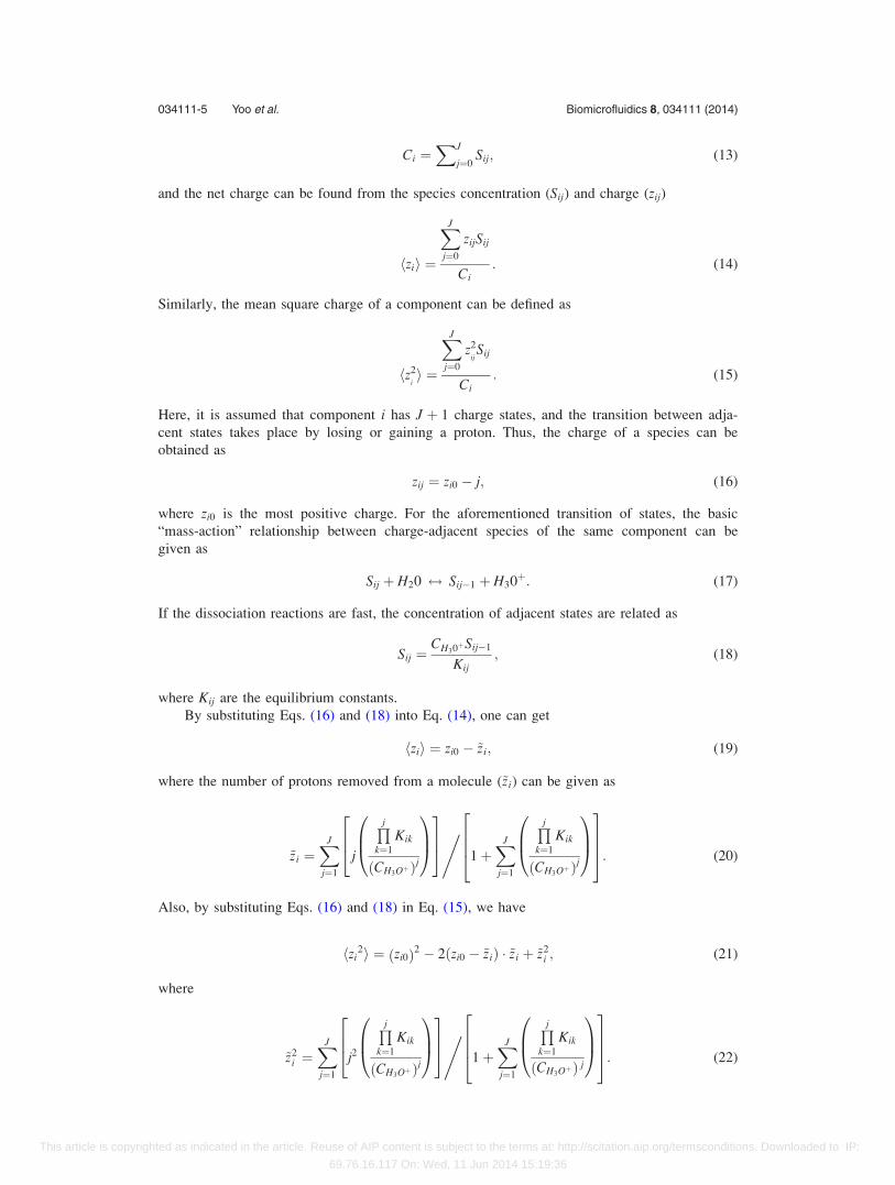
Ci ¼XJ
j¼0Sij; (13)
and the net charge can be found from the species concentration (Sij) and charge (zij)
hzii ¼
XJ
j¼0
zijSij
Ci: (14)
Similarly, the mean square charge of a component can be defined as
hz2ii ¼
XJ
j¼0
z2ijSij
Ci: (15)
Here, it is assumed that component i has J þ 1 charge states, and the transition between adja-
cent states takes place by losing or gaining a proton. Thus, the charge of a species can be
obtained as
zij ¼ zi0 � j; (16)
where zi0 is the most positive charge. For the aforementioned transition of states, the basic
“mass-action” relationship between charge-adjacent species of the same component can be
given as
Sij þ H20 $ Sij�1 þ H30þ: (17)
If the dissociation reactions are fast, the concentration of adjacent states are related as
Sij ¼CH30þSij�1
Kij; (18)
where Kij are the equilibrium constants.
By substituting Eqs. (16) and (18) into Eq. (14), one can get
hzii ¼ zi0 � ~zi; (19)
where the number of protons removed from a molecule (~zi) can be given as
~zi ¼XJ
j¼1
j
Qjk¼1
Kik
CH3Oþð Þj
0B@
1CA
264
375,
1þXJ
j¼1
Qjk¼1
Kik
CH3Oþð Þj
0B@
1CA
2664
3775: (20)
Also, by substituting Eqs. (16) and (18) in Eq. (15), we have
hzi2i ¼ zi0ð Þ2 � 2 zi0 � ~zið Þ � ~zi þ ~z2
i ; (21)
where
~z2i ¼
XJ
j¼1
j2
Qjk¼1
Kik
CH3Oþð Þj
0B@
1CA
264
375,
1þXJ
j¼1
Qjk¼1
Kik
CH3Oþð Þ j
0B@
1CA
2664
3775: (22)
034111-5 Yoo et al. Biomicrofluidics 8, 034111 (2014)
This article is copyrighted as indicated in the article. Reuse of AIP content is subject to the terms at: http://scitation.aip.org/termsconditions. Downloaded to IP:
69.76.16.117 On: Wed, 11 Jun 2014 15:19:36

The aforementioned methods for finding the net charge and mean square charge are applicable for
low molecular weight ampholytic components, such as the carrier ampholytes, for which the equilib-
rium constants (Ks) are known. However, for most proteins, the reaction rate constants are not readily
available. Rather titration curve can be constructed easily for most proteins. Once a titration curve is
known from the structure of the protein, the net charge is an explicit function of pH
hzii ¼ gi pHð Þ: (23)
Thus, from the knowledge of pH at a location, the net charge of a protein can be obtained. The
method of finding the mean square charge is more intricate. Mosher et al.15 presented a tech-
nique to find the mean square charge of a protein from a titration curve as
hz2i i ¼ hzii½ � 2 � 1
ln 10
dhziidpH
: (24)
C. Simplified mathematical model for FFIEF
In FFIEF, the concentration of other ionic components such as hydrogen (H) and hydroxyl
(OH) ions can also be described by Nernst-Planck equation. In that case, one has to solve Mpartial differential equations for the concentration of each component in the system in addition
to the charge conservation equation for the electric field. Though the numerical scheme needed
for solving the concentrations of hydrogen and hydronium ions is similar to any other mass
conservation (Nernst-Planck) equations, the convergence of solutions is very challenging for
hydrogen and hydronium ions because of 4–6 orders difference in magnitude in their concentra-
tion value. Thus, to circumvent the numerical stiffness, one can use the electroneutrality condi-
tion to find the concentration of hydrogen ion (CH) as
XM�2
i¼1
hziiDirCið Þ þ CH �KW
CH¼ 0; (25)
where Kw is the equilibrium constant for water. Here, the first term considers the contributions
of all amphoteric molecules (both proteins and ampholytes), while the second and third terms
are due to hydrogen and hydronium ions, respectively. From electroneutrality, the last term of
charge conservation equation (Eq. (12)) is also dropped out, and the modified charge conserva-
tion equation can be rewritten as
r � �kr/� FXN
i¼1
hziiDirCið Þ þ DHrCH � DOHrKW
CH
" #( )¼ 0: (26)
Here, ionic conductivity (k) is defined as
k ¼ FXN
i¼1
hzii2xiCi þ xHCH þ xOHKW
CH
" #: (27)
It is noteworthy to mention that the electroneutrality condition is not valid close to the wall
where the electric double layer might form. Thus, for nanochannel free flow IEF, one has to
solve the Poisson-Nernst-Planck model.16,17 However, in this study, the length scale of the elec-
tric double layer is 3–4 orders of magnitude smaller than the length scale of typical microfluidic
device used for FFIEF. Moreover, IEF channels are generally coated with chemicals to elimi-
nate the electric double layer formation.18,19 Using electroneutrality equation, the momentum
conservation equation can be rewritten as
�rpþ lr2~V ¼ 0: (28)
034111-6 Yoo et al. Biomicrofluidics 8, 034111 (2014)
This article is copyrighted as indicated in the article. Reuse of AIP content is subject to the terms at: http://scitation.aip.org/termsconditions. Downloaded to IP:
69.76.16.117 On: Wed, 11 Jun 2014 15:19:36

Thus, the complete mathematical description for FFIEF consists of Eqs. (2) and (28) for fluid
flow; Eqs. (9) and (25) for concentration of amphoteric components and hydrogen ions; and
Eq. (26) for electric potential.
D. Numerical scheme
The numerical algorithm used to calculate the flow velocity, concentration of amphoteric
component, and electric potential is shown in Figure 2. In this study, the discretized algebraic
equations are derived for mass, momentum, and charge conservation equations using finite vol-
ume method.20,21 The power law scheme is used to compute the flux terms in all equations.
The unsteady term in Nernst-Planck equation is modeled with a first order accurate implicit
scheme. For the fluid flow equations, the co-located semi-implicit method for pressure linked
equations (cSIMPLE) algorithm22 is used to find the pressure and velocity fields through an
iterative scheme. In this work, the system of linear algebraic equations is solved using line by
line Thomas algorithm23,24 owing to the tri-diagonal matrix system. The convergence tolerances
are 10�4 for continuity and momentum equations and 10�5 for mass and charge conservation
equations. To reduce the computational time, we have developed a parallel algorithm14 using
OpenMP.25 Numerical simulations are performed on an Intel Xeon 2.3 GHz (16 threads) and
each simulation result is obtained in 5 days.
III. RESULTS AND DISCUSSION
A. Model verification
To verify the FFIEF model, we compare our numerical results with the experimental find-
ings of Kohlheyer et al.,5 where they have presented the concept of free flow IEF in a straight
FIG. 2. The numerical algorithm for simulation of FFIEF. Here, Cni and /n are the concentration of each component i and
electric potential at nth iteration step.
034111-7 Yoo et al. Biomicrofluidics 8, 034111 (2014)
This article is copyrighted as indicated in the article. Reuse of AIP content is subject to the terms at: http://scitation.aip.org/termsconditions. Downloaded to IP:
69.76.16.117 On: Wed, 11 Jun 2014 15:19:36

microchannel. Unlike the experimental work of Cabrera and Yauger,4 a sheath flow of H2SO4
and NaOH was introduced in the anodic and cathodic sides to avoid the bubble formation.
These sheath flows eliminated the bubble formation problem in IEF, but it did not affect the
sample separation phenomena. Stable pH gradient formation was demonstrated in their micro-
channel using an applied electric field of 200 V/cm. Figure 3(a) (symbols) shows an almost lin-
ear pH profile at the end of their microchannel, where the pH values were obtained from the
locations of 7 pI markers used in their experimental study.5,6
To validate our model, we have simulated an identical case considering the 7 pI markers
used in the experimental work of Kohlheyer et al.5 The physico-chemical properties of pImarkers are listed in Table II. The pH gradient is created using 48 biprotic (DpK¼ 2.5) ampho-
lytes24 having isoelectric points between pH of 3.7 and 10.3. In other words, 48 mass conserva-
tion equations are solved to create the pH distribution for isoelectric focusing of proteins. It is
important to note that an increase in the number of ampholytes will make a smoother pH pro-
file for IEF. But we kept the number of ampholytes below 50 to keep the computational
expenses reasonable for multidimensional IEF.
The numerical simulation is only carried out in the effective separation chamber (5 mm
� 0.8 mm � 10 lm), where there is no influence of the sheath flow. Thus, there is no need to
consider the effect of acid and base in the numerical model simplifying the calculation. The pH
FIG. 3. (a) pH distributions across the channel at the channel outlet. Here symbols are from the experimental data of
Kohlheyer et al.5 for a FFIEF channel, while the solid lines are from the numerical results of an identical system. The con-
centration contours of pI markers from (b) experimental work (Reproduced with permission from Kohlheyer et al., Anal.
Chem. 79, 8190 (2007). Copyright 2007 American Chemical Society) and (c) numerical simulation work. The pI makers,
which are uniformly introduced at channel inlet, are concentrated at their isoelectric points and fully separated at the chan-
nel outlet. Depending on the pattern of separation, FFIEF column can be divided into separation and concentration zones.
The applied (nominal) electric field is 200 V/cm and the mean flow velocity is 1 mm/s.
034111-8 Yoo et al. Biomicrofluidics 8, 034111 (2014)
This article is copyrighted as indicated in the article. Reuse of AIP content is subject to the terms at: http://scitation.aip.org/termsconditions. Downloaded to IP:
69.76.16.117 On: Wed, 11 Jun 2014 15:19:36

distributions obtained from the numerical results are presented on Figure 3(a) as solid lines.
The numerical results show that the pH profile is not linear near the entry (x¼ 1 mm) region,
but a linear pH profile can be formed as the buffer solution flows downstream. Our numerical
results indicate that a stable and linear pH profile can be achieved within the 2 mm of the chan-
nel entry for a flow velocity of 1 mm/s. The numerical results agree well with the experimental
observations verifying the model developed here.
We also qualitatively validate the location of pI markers used in the experimental work of
Kohlheyer et al.5 Figure 3(b) shows the locale of experimental pI markers in the channel, while
the Figure 3(c) shows our numerical predictions with the same conditions. The contour plots
show similar trends in both experimental and numerical works of FFIEF. It is important to note
that a uniform mixture of pI markers is introduced at the entry region of the channel along with
a soup of carrier ampholytes. The pI markers are separated as the buffers moved downstream
with flow and each maker is totally separated at or near the isoelectric point at the end of chan-
nel (see Figure 3(c)). Based on the separation pattern, the FFIEF channel can be classified into
the separation zone and concentration zone. In the separation zone, lateral position of isoelectric
point is changing as samples are flowing downstream. On the other hand, in the concentration
zone, samples are concentrated at their isoelectric points without any further change in their lat-
eral positions (see Figures 3(b) and 3(c)).
B. Protein separation in a straight microchannel
In this section, we present the protein separation capability of FFIEF in a straight micro-
channel. The numerical simulations of FFIEF are carried out in a 6 mm (long) � 3 mm (wide)
channel considering two proteins: cardiac troponin I and serum albumin. The pH gradient in
the channel is formed using 48 carrier ampholytes (DpK¼ 2.5), and the isoelectric points of
these ampholytes are within the pH range of 5–8. Transport properties of carrier ampholytes,
proteins, and other ionic components are listed in Table III. The net charge values of serum al-
bumin and cardiac troponin I (cTnI) are obtained from the protein data bank26,27 for different
pH, and the titration curves are constructed using the Fourier series which are presented in
TABLE II. Physico-chemical parameters for pI markers used in Ref. 5.
pK1 pK2 pI x [m2/Vs]
pI marker 1 3.20 4.80 4.00 3.0� 10�8
pI marker 2 3.94 6.30 5.12 3.0� 10�8
pI marker 3 5.35 6.95 6.15 3.0� 10�8
pI marker 4 6.20 8.10 7.15 3.0� 10�8
pI marker 5 6.80 9.30 8.05 3.0� 10�8
pI marker 6 8.05 9.85 8.95 3.0� 10�8
pI marker 7 9.95 10.65 10.30 3.0� 10�8
TABLE III. Physico-chemical parameters for ampholytes, proteins, hydrogen ions, and hydroxyl ions.
Buffer solution dynamic viscosity l 1.002 [mPa-s]
Electrophoretic
mobility
Ampholyte xamp 3� 10�8[m2/V-s]
cTnI xcTnI 1:56� 10�8[m2/V-s]29
Albumin xALB 2:0� 10�8[m2/V-s]29
Hydrogen ion xHþ 36:25� 10�8[m2/V-s]30
Hydroxyl ion xOH� 20:50� 10�8[m2/V-s]30
Diffusivity of components Di xiRT=F[m2/s]
Dissociation constant of proton ion in water solution KW 1:0� 10�14 (molarity based)
034111-9 Yoo et al. Biomicrofluidics 8, 034111 (2014)
This article is copyrighted as indicated in the article. Reuse of AIP content is subject to the terms at: http://scitation.aip.org/termsconditions. Downloaded to IP:
69.76.16.117 On: Wed, 11 Jun 2014 15:19:36

Figure 4. These titration curves are used to find the mean square charge of proteins using
Eq. (24).
The buffer solution of carrier ampholytes is first introduced in the separation channel at a
flow velocity of 1 mm/s, and a potential difference of 80 V is applied between anodic and ca-
thodic sides to form the pH gradient in the channel. Figures 5(a) and 5(b) show the pH profile
in the separation channel at the end of the stabilization phase. Here, the stabilization phase is
similar to steady state when the pH profile in the channel does not change with time. Near the
channel entry, the pH profile is quite nonlinear as ampholytes are moving due to advection and
trying to focus at their isoelectric points due to electromigration. But at the end of the channel,
a nearly linear pH profile (see Figure 5(b)) is formed which is very conducive for separation of
proteins.
At the end of the (ampholyte) stabilization phase, a uniform mixture of sample proteins is
introduced to the separation channel continuously. This is very similar to the experimental
work of Cheng and Chang9 in which they introduced the sample mixture in the separation chan-
nel after forming the pH profile using an actuator. Figure 5(c) shows the protein concentration
FIG. 4. Titration curves for (a) human serum albumin and (b) cTnI (adult cardiac troponin I). The pI points for serum albu-
min and cTnI are 6.29 and 6.96, respectively. The titration curves used in this study are formed from the protein sequence.
First, the sequence of a particular protein is obtained from UniProt.26 Next, the protein sequence is exported to a protein
calculator27 to obtain charge distribution at different pH values. In this study, a Fourier series is used to form the smooth ti-
tration curves from charge data. The titration curve is used subsequently to find net charges and mean square charges.
034111-10 Yoo et al. Biomicrofluidics 8, 034111 (2014)
This article is copyrighted as indicated in the article. Reuse of AIP content is subject to the terms at: http://scitation.aip.org/termsconditions. Downloaded to IP:
69.76.16.117 On: Wed, 11 Jun 2014 15:19:36
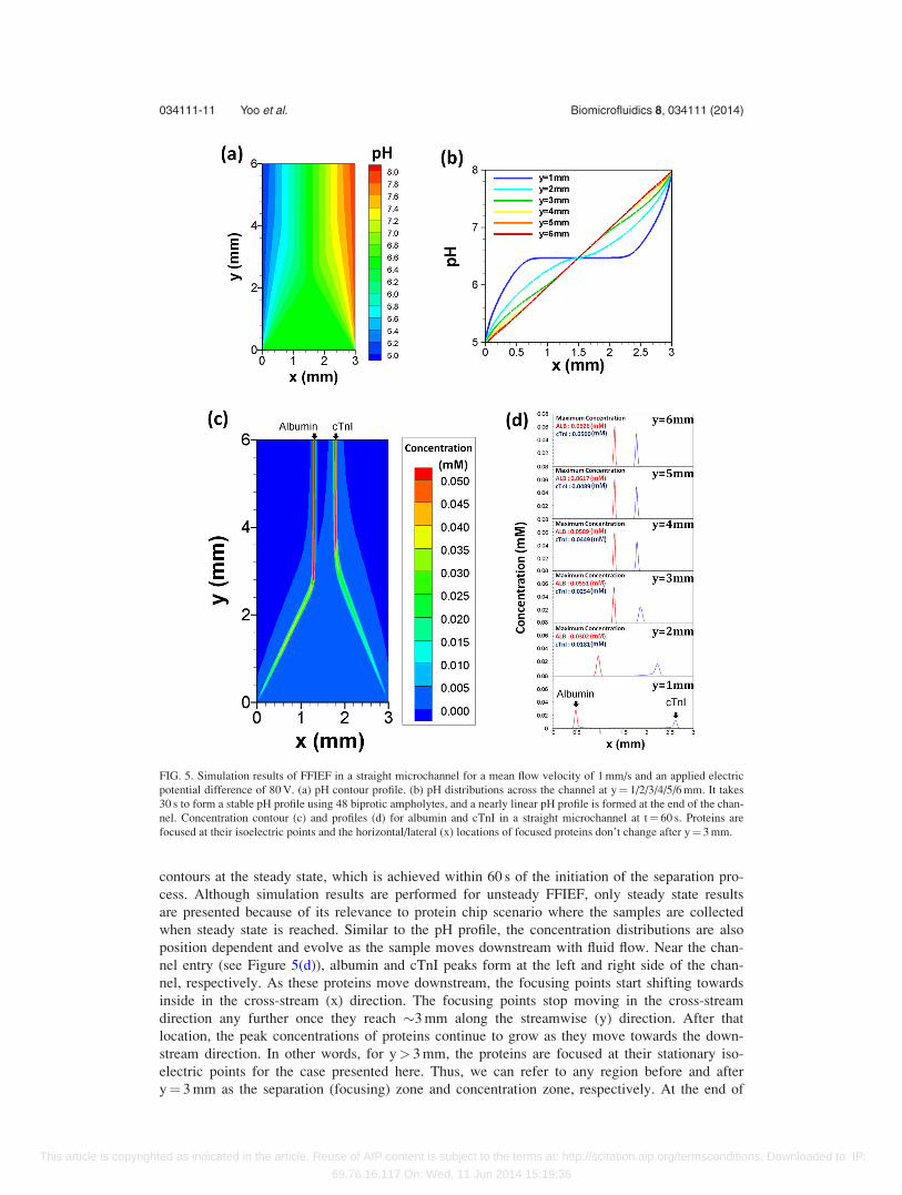
contours at the steady state, which is achieved within 60 s of the initiation of the separation pro-
cess. Although simulation results are performed for unsteady FFIEF, only steady state results
are presented because of its relevance to protein chip scenario where the samples are collected
when steady state is reached. Similar to the pH profile, the concentration distributions are also
position dependent and evolve as the sample moves downstream with fluid flow. Near the chan-
nel entry (see Figure 5(d)), albumin and cTnI peaks form at the left and right side of the chan-
nel, respectively. As these proteins move downstream, the focusing points start shifting towards
inside in the cross-stream (x) direction. The focusing points stop moving in the cross-stream
direction any further once they reach �3 mm along the streamwise (y) direction. After that
location, the peak concentrations of proteins continue to grow as they move towards the down-
stream direction. In other words, for y> 3 mm, the proteins are focused at their stationary iso-
electric points for the case presented here. Thus, we can refer to any region before and after
y¼ 3 mm as the separation (focusing) zone and concentration zone, respectively. At the end of
FIG. 5. Simulation results of FFIEF in a straight microchannel for a mean flow velocity of 1 mm/s and an applied electric
potential difference of 80 V. (a) pH contour profile. (b) pH distributions across the channel at y¼ 1/2/3/4/5/6 mm. It takes
30 s to form a stable pH profile using 48 biprotic ampholytes, and a nearly linear pH profile is formed at the end of the chan-
nel. Concentration contour (c) and profiles (d) for albumin and cTnI in a straight microchannel at t¼ 60 s. Proteins are
focused at their isoelectric points and the horizontal/lateral (x) locations of focused proteins don’t change after y¼ 3 mm.
034111-11 Yoo et al. Biomicrofluidics 8, 034111 (2014)
This article is copyrighted as indicated in the article. Reuse of AIP content is subject to the terms at: http://scitation.aip.org/termsconditions. Downloaded to IP:
69.76.16.117 On: Wed, 11 Jun 2014 15:19:36

the channel, the concentrations of albumin and cTnI have increased 54 and 47 fold, respec-
tively, from their initial values. Albumin forms tighter bands compared to cTnI because the
slope of the titration curve is steeper for albumin compared to cTnI (see Figure 4). The simula-
tion result also reveals that two proteins can be totally separated near the channel outlet.
To investigate the effect of the applied electric field in the protein separation phenomena,
FFIEF simulations are carried out for different applied electric field scenarios. The applied elec-
tric potential difference between anode and cathode sides are varied between 40 V and 160 V,
while keeping all other simulation conditions the same as discussed in Sec. III B. The concen-
tration contours of albumin and cTnI proteins are shown in Figure 6 for nominal electric field
of 133.3 V/cm and 533.3 V/cm. Simulation results indicate that the length of the focusing zone
is shorter as the applied electric field is increased. For instance, the length of the focusing zone
is 6 cm for a nominal electric field of 133.3 V/cm, while this value is 3 cm and 1.5 cm for nomi-
nal electric field of 266.7 V/cm and 533.3 V/cm, respectively. Moreover, the protein peak con-
centration highly depends on applied electric potential difference. In particular, for lower
applied electric field (Figure 6(a)) proteins are still focusing near the channel outlet as evi-
denced by the changes in the peak concentration locations. Therefore, an adequate electric field
should be applied to complete the focusing within the channel length. Higher applied electric
field will ensure complete separation of proteins in addition to providing tightly focused protein
bands. However, a higher electric field will result in significant Joule heating in the system
which may adversely affect the protein separation performance.28
C. A new channel design for high resolution FFIEF separation
In protein separation work, the performance of a separation process is estimated by the re-
solution. The separation resolution (Rij) between two proteins (i and j) can be estimated as
Rij ¼jxf ;i � xf ;jj2ri þ 2rj
; (29)
where xf and r are the location of concentration peak and the standard deviation of concentra-
tion band, respectively. Equation (29) indicates that the tightly focused protein bands and/or a
large separation distance between peak points can ensure high resolution. As shown earlier, the
tightly formed protein bands can be formed using higher electric field. However, there is an
upper limit on applied electric field strength since the proteins might be denatured at high
FIG. 6. Effect of applied electric field in the pH formation. Protein concentration contours for an applied electric potential
difference of (a) 40 V and (b) 160 V. All other simulation conditions are the same as in Figure 5. The length of focusing
zone is reduced as applied electric potential difference is increased.
034111-12 Yoo et al. Biomicrofluidics 8, 034111 (2014)
This article is copyrighted as indicated in the article. Reuse of AIP content is subject to the terms at: http://scitation.aip.org/termsconditions. Downloaded to IP:
69.76.16.117 On: Wed, 11 Jun 2014 15:19:36

temperature due to Joule heating. An alternative approach to improve the resolution is to
increase the distance between the focused protein peaks. In a straight channel, the focused (iso-
electric) point for a protein is primarily determined by the pH profile formed by the carrier
ampholytes, and a laminar flow cannot change the pI locations appreciably. In a straight chan-
nel, the streamwise flow (not shown) becomes parabolic (in the z-direction) at the end of the
separation channel, and there is no noticeable cross-stream flow velocity (Figure 7(b)) for any
influence on the change in the location of pI points. However, the flow velocity can be per-
turbed by introducing a channel insert/post at the end of the separation channel. Figures 7(c)
and 7(d) show the streamwise and cross-stream velocity distributions along a microchannel
when a post/block is placed at the end of the channel between x¼ 1 mm and x¼ 2 mm. This
post blocks 1/3 of the flow area compared with the case shown in Figures 7(a) and 7(b) where
the channel is fully open. Moreover, this post creates significant cross-stream velocity, which
can be exploited to increase the focusing distance between the two adjacent protein bands.
Figure 8 shows the effect of cross-stream flow on the sample separation and concentration
in FFIEF channel where a flow block is inserted at the channel exit. The behavior of pH forma-
tion and protein separation is similar to fully open channel (Figure 5) until y¼ 4 mm. Beyond
that point the effect of cross-stream flow becomes important and it makes a significant change
in the isoelectric focusing process. Figure 8(b) shows that the pH profile becomes flat at the
end of the separation channel when a block is introduced at the end of the channel. This flat
pH profile increases the physical distance between two pI points, which essentially increase the
distance between two protein bands (Figure 8(d)). Unlike the fully open channel case presented
FIG. 7. Flow velocity distribution in FFIEF channels. Streamwise (a) and cross-stream (b) velocity for a separation channel
(6 mm � 3 mm � 10 lm) used for Figures 5 and 6. There is no noticeable cross-stream velocity at the downstream of a
straight microchannel due to fully developed low Reynolds number creeping flow. Streamwise (c) and cross-stream (d) ve-
locity for a higher resolution separation channel (6 mm � 3 mm � 10 lm). Cross-stream velocities are created by partially
blocking the channel exit between x¼ 1 mm and x¼ 2 mm. These cross-stream velocities are exploited to increase the sepa-
ration resolution by increasing the separation distance between focused peaks.
034111-13 Yoo et al. Biomicrofluidics 8, 034111 (2014)
This article is copyrighted as indicated in the article. Reuse of AIP content is subject to the terms at: http://scitation.aip.org/termsconditions. Downloaded to IP:
69.76.16.117 On: Wed, 11 Jun 2014 15:19:36

in Figure 5(d), the separation distance between the two proteins decreases during the focusing
phase, while it increases during the concentration phase. Although the cross-stream flow
increases the distance between the focused proteins, it reduces the concentration of protein
peak. However, the effect of reduction in peak height is much less compared with the increase
in separation distance. To quantify the relative merits and pitfalls of the new design, the separa-
tion resolution is presented in Figure 9 for both fully open channel (case A) and the channel
partly blocked at the exit (case B). For the fully open case, the resolution increases until
y¼ 4 mm due to the focusing of proteins at their pI points, while decreases slightly afterwards
due to decrease in the focusing distance while maintaining the peak width and height. On the
other hand, for case B, the resolution decreases first due to the decrease in separation distance,
but increases after y¼ 4 mm due to the increase in separation distance due to cross-flow.
Figure 9 shows that the resolution increases three folds once the cross-stream velocity is intro-
duced using a post/block at the channel exit. This simple design is very helpful to increase the
separation distance while maintaining relatively low electric field strength.
FIG. 8. Simulation results of FFIEF in a high resolution separation channel for a mean flow velocity of 1 mm/s and an
applied electric potential difference of 80 V. (a) pH contour profile. (b) pH distribution across the channel at
y¼ 1/2/3/4/5/6 mm. It takes 60 s to form a stable pH profile using 48 biprotic ampholytes, and a nearly flat pH profile is
formed at the mid section of the channel exit due to flow blockage. Concentration contour (c) and profiles (d) for albumin
and cTnI at t¼ 120 s.
034111-14 Yoo et al. Biomicrofluidics 8, 034111 (2014)
This article is copyrighted as indicated in the article. Reuse of AIP content is subject to the terms at: http://scitation.aip.org/termsconditions. Downloaded to IP:
69.76.16.117 On: Wed, 11 Jun 2014 15:19:36

Although the channel design presented in case B uses the identical isoelectric focusing con-
ditions (number of ampholytes, applied electric field, etc.) as in case A, the fluid flow condition
is quite different in case B. The flow blockage caused by the post results in a higher pressure
drop in case B compare to case A as shown in Figure 10. Therefore, one has to use high pump-
ing power to operate case B configuration. More importantly, it takes longer time to obtain the
focusing and separation. For instance, the stabilization and separation times are 30 s and 60 s
for fully open channel case A, while it takes 60 s to form stable pH profile and 2 min for com-
plete separation of cTnI and albumin in case B. Nevertheless, the insertion of a post at the
channel exit can be exploited to increase the separation resolution. This is especially useful for
separation of proteins having much closer pI points. However, in this case the position of the
post has to be adjusted based on the pI points of proteins. Figure 11 shows the concentration
distribution of two proteins (Hemoglobin subunit B (HBB) and G (HBG)) in a microchannel
for a nominal applied electric field of 266.7 V/cm and an inlet flow velocity of 1 mm/s. In this
case, the final focused points of both proteins are located at the right half of the channel when
no post is used (Figure 11 (left)). However, the final separation distance as well as the
FIG. 9. FFIEF separation performance for fully open separation channel (case A) and partially blocked separation channel
(case B).
FIG. 10. Pressure distribution along the separation channel for fully open and partially blocked outlet. The maximum pres-
sure drops for fully open and partially blocked outlet are 695 Pa and 712 Pa, respectively.
034111-15 Yoo et al. Biomicrofluidics 8, 034111 (2014)
This article is copyrighted as indicated in the article. Reuse of AIP content is subject to the terms at: http://scitation.aip.org/termsconditions. Downloaded to IP:
69.76.16.117 On: Wed, 11 Jun 2014 15:19:36

separation resolution can be improved significantly by placing a block between x¼ 1.5 mm and
x¼ 2.6 mm (Figure 11 (right)). The separation resolution of proteins having very close isoelec-
tric points can be improved by reducing the width of the separation post (not shown) as well as
by using narrow pH range for ampholytes.
IV. SUMMARY AND CONCLUSIONS
A mathematical model is developed to simulate the FFIEF considering the mass, momen-
tum, and charge conservation equations. The governing partial differential equations are solved
using the co-located finite volume method. To obtain numerical simulation results in a reasona-
ble time, an in house numerical code is developed using OpenMP based parallel scheme.
Numerical results obtained from this model are compared with the existing experimental work;
an excellent agreement is obtained between numerical and experimental work where pH profile
development and separation of pI markers are considered. Numerical simulations are carried
out for FFIEF considering 48 ampholytes and 2 real proteins for an applied electric field range
of 133 V/cm to 533 V/cm. The electric field is introduced to focus carrier ampholytes and pro-
teins at their isoelectric points. The focused ampholytes first formed the required pH profile in
the system for the separation of proteins from an initial uniform mix, while the flow field is
applied to collect the separated proteins. The numerical results reveal that the pH profile is
formed as buffer solution goes downstream and analytes can be totally separated at the channel
outlet.
The effects of electric and flow fields are particularly considered in this study. The flow
field effect is introduced by changing the channel design. Two different channel designs are
considered in this study. The first design is based on a straight microchannel, while, in the sec-
ond design, a post is inserted at the end of a straight microchannel to disturb the flow. The fully
open outlet channel in the first design produces parabolic streamwise velocity, but no cross-
stream velocity at the end of the channel. On the other hand, the partially blocked outlet in the
second design creates significant cross-flow which improves the separation resolution by
increasing the separation distance between the focused peaks. Even though no changes in the
electrochemical condition are needed in the second design to achieve higher resolution, the
pumping pressure drop is little higher in the second design. Moreover, it takes longer time in
the second design for formation of stable pH profile as well as separation of proteins. The
FIG. 11. Simulation results of FFIEF for fully open (case A) and partially blocked (case B) channel. The numerical simula-
tions of FFIEF are carried out in a 6 cm (long) � 3 cm (wide) channel considering two proteins: Hemoglobin (subunit) B
(HBB) and G (HBG). The isoelectric points of HBB and HBG are 7.27 and 8.21, respectively. The pH gradient in the chan-
nel is formed using 48 carrier ampholytes having DpK of 2.5, and the isoelectric points of these ampholytes are within the
pH range of 5–9. The inlet flow velocity is 1 mm/s. A nominal electric field of 266.7 V/cm is applied to form the pH gradi-
ent in the channel. Here, the pressure drop between inlet and outlet are 695 Pa and 716 Pa for case A and case B, respec-
tively. The separation resolution is 7.9 and 11.7 for fully open (case A) and for partially blocked (case B), respectively.
034111-16 Yoo et al. Biomicrofluidics 8, 034111 (2014)
This article is copyrighted as indicated in the article. Reuse of AIP content is subject to the terms at: http://scitation.aip.org/termsconditions. Downloaded to IP:
69.76.16.117 On: Wed, 11 Jun 2014 15:19:36

applied electric field strength has direct effect on higher separation resolution and shorter chan-
nel length. However, higher electric field might cause dispersion in separated proteins as well
as denaturation of proteins due to elevated temperature.
ACKNOWLEDGMENTS
This work was supported in part by the US National Science Foundation under Grant No.
CBET 1250107.
1K. Hannig, Fresenius’ J. Anal. Chem. 181, 244 (1961).2H. Wagner, Nature 341, 669 (1989).3L. Krivankova and P. Bocek, Electrophoresis 19, 1064 (1998).4C. R. Cabrera and P. Yager, Electrophoresis 22, 355 (2001).5D. Kohlheyer, J. C. T. Eijkel, S. Schlautmann, A. van den Berg, and R. B. M. Schasfoort, Anal. Chem. 79, 8190 (2007).6D. Kohlheyer, J. C. T. Eijkel, S. Schlautmann, A. van den Berg, and R. B. M. Schasfoort, Anal. Chem. 80, 4111 (2008).7J. Wen, J. W. Albrecht, and K. F. Jensen, Electrophoresis 31, 1606 (2010).8J. Wen, E. W. Wilker, M. B. Yaffe, and K. F. Jensen, Anal. Chem. 82, 1253 (2010).9L. J. Cheng and H. C. Chang, Lab Chip 14, 979 (2014).
10L. J. Cheng and H. C. Chang, Biomicrofluidics 5, 046502 (2011).11M. W. Frank and F. M. White, Fluid Mechanics (McGraw-Hill, New York, New York, 1979).12J. S. Newman, Electrochemical Systems (Prentice-Hall, Englewood Cliffs, NJ, 1972).13A. P. S. Bhalla, R. Bale, B. E. Griffith, and N. A. Patankar, J. Comput. Phys. 256, 88 (2014).14K. Yoo, J. Shim, J. Liu, and P. Dutta, Electrophoresis 35, 638 (2014).15R. A. Mosher, D. A. Saville, and W. Thormann, The Dynamics of Electrophoresis (VCH, Weinheim; New York, 1992).16M. Pribyl, D. Snita, and M. Marek, Chem. Eng. J. 105, 99 (2005).17J. Lindner, D. Snita, and M. Marek, Phys. Chem. Chem. Phys. 4, 1348 (2002).18H. C. Cui, K. Horiuchi, P. Dutta, and C. F. Ivory, Anal. Chem. 77, 1303 (2005).19H. C. Cui, K. Horiuchi, P. Dutta, and C. F. Ivory, Anal. Chem. 77, 7878 (2005).20J. Shim, P. Dutta, and C. F. Ivory, Electrophoresis 28, 572 (2007).21J. Shim, P. Dutta, and C. F. Ivory, Numer. Heat Trans. 52, 441 (2007).22T.-K. J. Sze, J. Liu, and P. Dutta, J. Fluids Eng. 136, 021206 (2013).23J. Shim, P. Dutta, and C. F. Ivory, Electrophoresis 29, 1026 (2008).24J. Shim, P. Dutta, and C. F. Ivory, J. Nanosci. Nanotechnol. 8, 3719 (2008).25R. Chandra, Parallel Programming in OpenMP (Morgan Kaufmann Publishers, San Francisco, CA, 2001).26See http://www.uniprot.org for UniProt, March 3, 2009 edition.27C. Putnam, 3.3 ed., http://www.scripps.edu/�cdputnam, 2006.28A. S. Rathore, J. Chromatogr. A 1037, 431 (2004).29D. Bottenus, M. R. Hossan, Y. Ouyang, W.-J. Dong, P. Dutta, and C. F. Ivory, Lab Chip 11, 3793 (2011).30A. B. Duso and D. D. Y. Chen, Anal. Chem. 74, 2938 (2002).
034111-17 Yoo et al. Biomicrofluidics 8, 034111 (2014)
This article is copyrighted as indicated in the article. Reuse of AIP content is subject to the terms at: http://scitation.aip.org/termsconditions. Downloaded to IP:
69.76.16.117 On: Wed, 11 Jun 2014 15:19:36